core.ac.uk · linear algebra and its applications 433 (2010) 447–475 contents lists available at...
TRANSCRIPT

Linear Algebra and its Applications 433 (2010) 447–475
Contents lists available at ScienceDirect
Linear Algebra and its Applications
j ourna l homepage: www.e lsev ie r .com/ loca te / laa
Cauchy-type determinants and integrable systems
Cornelia Schiebold
Department of Mathematics, Mid Sweden University, S-851 70 Sundsvall, Sweden
A R T I C L E I N F O A B S T R A C T
Article history:
Received 19 January 2010
Accepted 7 March 2010
Available online 8 April 2010
Submitted by A. Böttcher
AMS classification:
15A15
35Q51
37K40
37K30
Keywords:
Cauchy-type determinants
Sylvester equation
Integrable systems
Multiple pole solutions
It iswell knownthat theSylvestermatrixequationAX + XB = C has
a unique solution X if and only if 0 /∈ spec(A)+ spec(B). The main
result of thepresent article areexplicit formulas for thedeterminant
of X in the case that C is one-dimensional. For diagonal matrices A,
B, we reobtain a classical result by Cauchy as a special case.
The formulas we obtain are a cornerstone in the asymptotic clas-
sification of multiple pole solutions to integrable systems like the
sine-GordonequationandtheToda lattice.Wewillprovideaconcise
introduction to the background from soliton theory, an operator
theoretic approach originating from work of Marchenko and Carl,
and discuss examples for the application of the main results.
© 2010 Elsevier Inc. All rights reserved.
1. Introduction
In the present article we study the determinants of certain solutions to Sylvester’s equation, which
are relevant inmathematical physics. For givenmatrices A ∈ Mn,n(C), B ∈ Mm,m(C), not necessarilyof equal size, we consider the operatorΦA,B : Mn,m(C) → Mn,m(C) given by
ΦA,BX = AX + XB.
The equation AX + XB = C is also known as the Sylvester equation [29]. It is well known that
spec(ΦA,B) = spec(A)+ spec(B),
where the right-handsidedenotes theMinkowski sumof the twospectra. InparticularΦA,B is invertible
if and only if 0 /∈ spec(A)+ spec(B), see [2] for a survey and further references. A remarkable result on
E-mail address: [email protected]
0024-3795/$ - see front matter © 2010 Elsevier Inc. All rights reserved.
doi:10.1016/j.laa.2010.03.011

448 C. Schiebold / Linear Algebra and its Applications 433 (2010) 447–475
elementary operators (see [7,9]) implies that all this extends to the general setting of Banach operator
ideals.
In what followswewill always consider finitematrices A and B for whichΦA,B is invertible. Our aim
is to obtain formulas for det(Φ
−1A,B (C)
), for certain matrices C, which depend explicitly on the entries
of A, B and C. Of course it would be toomuch to hope for completely explicit formulas in full generality.
Before explainingwhich caseswe consider andwhy, let us recall the historically first result of the topic:
Taking for A = B = diagα1, . . . ,αn and for E the matrix with all entries equal to 1, one obtains
Φ−1A,B (E) =
(1
αi + αj
)ni,j=1
.
Then a classical result of Cauchy [6], see also [18], is that
det(Φ
−1A,B (E)
)=
n∏i=j
1
2αj
n∏i,j=1i<j
(αi − αj
αi + αj
)2.
Observe that the matrix E is one-dimensional, i.e. of rank one. We will usually write such operators in
tensor notation: For a, c ∈ Cn with a, c /= 0, the matrix a ⊗ c :=(ajci)ni,j=1 is one-dimensional, since
its range is the span of c. Note that conversely every one-dimensional matrix can be written in the
above form.
Our main results, the Theorems 4.8 and 5.2 will generalize Cauchy’s result by providing explicit
formulas for
det(Φ
−1A,B (a ⊗ c)
), (1.1)
det
(0 Φ
−1A,B (b ⊗ c)
Φ−1B,A (a ⊗ d) 0
), (1.2)
det
(0 Φ
−1A,B (b ⊗ c)
Φ−1B,A (a ⊗ d) −b ⊗ d
)(1.3)
for matrices A ∈ Mn,n(C), B ∈ Mm,m(C) in Jordan form and arbitrary vectors a, c ∈ Cn, b, d ∈ Cm.
In (1.1), the argument of Φ−1A,B is a one-dimensional matrix, as in Cauchy’s formula. The matrix in
(1.2) can be interpreted as the solution for an appropriate Sylvester equation with a two-dimensional
C (see Remark 1). Finally, the matrix in (1.3) is a perturbation of that in (1.2), which is important in
applications. The assumption that A, B are in Jordan form does not turn out to be very restrictive
in practice. Of course, the determinants (1.1), (1.2) and (1.3) change under transformation of A and B.
Howeverwe obtain explicit formulas, as soon as the determinants of thematrices transforming A and B
to Jordan formare known. For example, ifA = T−1JT , B = S−1KSwith J, K in Jordan form, one just uses
det(Φ
−1A,B (a ⊗ c)
)= det(S)
det(T)det(Φ−1
J,K
(((S−1)′a)⊗ (Tc)
)).
Themain reason to focus on these particular situations stems from the theory of integrable systems. It
has been known for a long time [12], see also [13,28], that Cauchy’s result is related to the asymptotic
behavior of N-solitons.
In Section 2 we give a concise introduction to determinant formulas for the solutions of integrable
systems, following an operator theoretic approach inspired by pioneeringwork ofMarchenko [14] and
developed by Carl and collaborators at Jena University [1,3,5,21]. These formulas incorporate solutions
to Sylvester’s equation and their determinants. The striking point is that, on the level of solutions and
their dynamics, the transition to Jordan form is very easy to understand and essentially negligible. Note
also that the solution formulas contain A and B as independent parameters, allowing us to transform
them independently. In Section 6 we will explain how our results on determinants are involved in the
complete asymptotic description of multiple pole solutions, a problem which had been open for at
least two decades and was only recently solved by the author [21,23,27].

C. Schiebold / Linear Algebra and its Applications 433 (2010) 447–475 449
In conclusion some remarks seem in order how we proceed to calculate the determinants (1.1),
(1.2) and (1.3). To grasp our strategy it may help to regard the matrices A, B as fixed and the vectors
a, c (or a, b, c, d) as variable. The first step is to write each of (1.1), (1.2) and (1.3) as a product γ det(U)where γ = γ (a, c) is an explicit polynomial in the entries of a, c (or of a, b, c, d), and U is a constant
matrix depending only on the eigenvalues ofA andB and theirmultiplicities. Such factorizationswill be
found in Section 3. Actually the matrices U we obtain are visibly generalizations of the matrix already
considered by Cauchy, but the calculation of their determinants will still require considerable effort.
The determinants (1.1) will be calculated in Section 4, (1.2) and (1.3) will be treated in Section 5.
2. Why to calculate determinants of inverse images of elementary operators
In this section we describe the link between Cauchy-type determinants and integrable systems,
which was our motivation to investigate the determinants (1.1), (1.2) and (1.3). A reader who is mainly
interested in determinant formulas themselves may skip this section without loss of continuity.
Let us start with the famous Korteweg–de Vries (KdV) equation
ut = uxxx + 6uux.
Although the KdV is nonlinear, it has a surprisingly well-behaved solution theory. For example, the
initial value problem is solvable for all times t ∈ R for rapidly decaying initial data u0(x). The usual
approach to the initial value problem is the inverse scattering method (see [10], and also [8] for an
introduction). On the other hand, much research is directed towards finding explicit expressions for
global solutions. In [1], the authors derive the solution formula
u(x, t) = 2∂2
∂x2log det
(I + exp(Ax + A3t)Φ−1
A,A (a ⊗ c)), (2.1)
where a ⊗ c denotes the one-dimensionalmatrix(ajci)ni,j=1
for a = (aj)nj=1, c = (cj)
nj=1 ∈ Cn (see also
[4] for KdV-type hierarchies). Using functional analysis, the formula can be generalized to include all
solutions of the usual inverse scattering method [3], see also [5].
Here we restrict ourselves to the matrix case. Taking for A diagonal matrices with n distinct eigen-
values one obtains the n-solitons, solutions which almost look like a linear superposition of n stable
solitary waves, which do not loose their shape in the collisions but suffer a phase shift. Shape, velocity
and interactionbehavior canbederived fromtheeigenvalues,where the computationof thephase shift
uses Cauchy’s result. The role of the one-dimensionalmatrix a ⊗ c is less interesting: It just determines
the position of the waves at time t = 0. Furthermore it can be shown that diagonizable matrices lead
to the same solutions as their diagonalizations. We will come back to admissible transformations of
matrices below when we discuss the solution formula of the KP equation.
Similarly the general matrix case reduces to matrices in Jordan form. This leads to the so-called
multiple pole solutions, which consist of groups of waves whose members are weakly bound (see
Section 6 for a discussion of examples). From the earlier literature on, discussion of these solutions
had been appearing occasionally (see for example [17,30,31]), mostly in very particular cases. But the
question of a complete and rigorous asymptotic characterization stems, to the best of our knowledge,
fromwork ofMatveev [16], who treated the related class of positons to a certain extent and formulated
expectations for the general case. In this spirit, particular cases of multiple pole solutions (called
negatons in this context) were examined in [19].
In [20–23,27], the author gave a complete and rigorous description of the multiple pole solutions
of the KdV, the Toda lattice, the sine-Gordon equation and the Nonlinear Schrödinger equation. For an
informal discussionof the resultwe refer to Section6,whereweexplain in several concrete examples in
whichway the determinants studied in the present work are used to discover the asymptotic behavior
of these solutions.
One of the most striking phenomena in the theory of integrable systems is that equations with
very different physical background can be treated by analogous methods (which does not exclude
major differences in the details). We do not have the space to explain the solution formulas for other
important soliton equations, which were found via our operator approach. Here it may suffice to list
which types of inverse images of elementary operators they contain. This can be read off from Table 1.
450 C. Schiebold / Linear Algebra and its Applications 433 (2010) 447–475
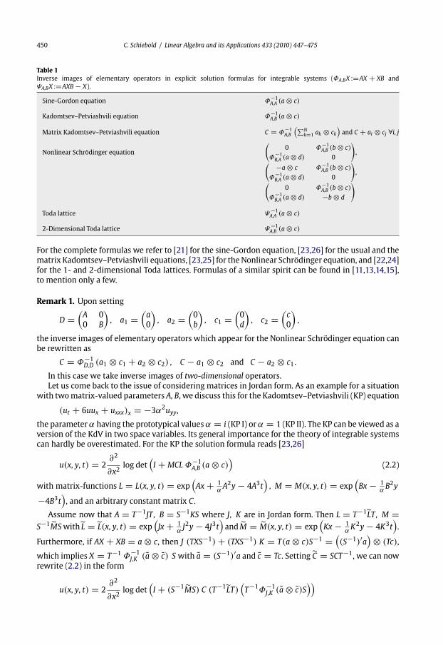
Table 1
Inverse images of elementary operators in explicit solution formulas for integrable systems (ΦA,BX :=AX + XB and
ΨA,BX :=AXB − X).
Sine-Gordon equation Φ−1A,A (a ⊗ c)
Kadomtsev–Petviashvili equation Φ−1A,B (a ⊗ c)
Matrix Kadomtsev–Petviashvili equation C = Φ−1A,B
(∑Nk=1 ak ⊗ ck
)and C + ai ⊗ cj ∀i, j
Nonlinear Schrödinger equation
(0 Φ
−1A,B (b ⊗ c)
Φ−1B,A (a ⊗ d) 0
),( −a ⊗ c Φ
−1A,B (b ⊗ c)
Φ−1B,A (a ⊗ d) 0
),(
0 Φ−1A,B (b ⊗ c)
Φ−1B,A (a ⊗ d) −b ⊗ d
)
Toda lattice Ψ−1A,A (a ⊗ c)
2-Dimensional Toda lattice Ψ−1A,B (a ⊗ c)
For the complete formulas we refer to [21] for the sine-Gordon equation, [23,26] for the usual and the
matrix Kadomtsev–Petviashvili equations, [23,25] for the Nonlinear Schrödinger equation, and [22,24]
for the 1- and 2-dimensional Toda lattices. Formulas of a similar spirit can be found in [11,13,14,15],
to mention only a few.
Remark 1. Upon setting
D =(A 0
0 B
), a1 =
(a
0
), a2 =
(0
b
), c1 =
(0
d
), c2 =
(c
0
),
the inverse images of elementary operators which appear for the Nonlinear Schrödinger equation can
be rewritten as
C = Φ−1D,D (a1 ⊗ c1 + a2 ⊗ c2) , C − a1 ⊗ c2 and C − a2 ⊗ c1.
In this case we take inverse images of two-dimensional operators.
Let us come back to the issue of considering matrices in Jordan form. As an example for a situation
with twomatrix-valued parameters A, B, we discuss this for the Kadomtsev–Petviashvili (KP) equation
(ut + 6uux + uxxx)x = −3α2uyy,
the parameterα having the prototypical valuesα = i (KP I) orα = 1 (KP II). The KP can be viewed as a
version of the KdV in two space variables. Its general importance for the theory of integrable systems
can hardly be overestimated. For the KP the solution formula reads [23,26]
u(x, y, t) = 2∂2
∂x2log det
(I + MCL Φ
−1A,B (a ⊗ c)
)(2.2)
with matrix-functions L = L(x, y, t) = exp(Ax + 1
αA2y − 4A3t
), M = M(x, y, t) = exp
(Bx − 1
αB2y
−4B3t), and an arbitrary constant matrix C.
Assume now that A = T−1JT , B = S−1KS where J, K are in Jordan form. Then L = T−1LT , M =S−1MSwith L = L(x, y, t) = exp
(Jx + 1
αJ2y − 4J3t
)and M = M(x, y, t) = exp
(Kx − 1
αK2y − 4K3t
).
Furthermore, if AX + XB = a ⊗ c, then J (TXS−1)+ (TXS−1) K = T(a ⊗ c)S−1 =((S−1)′a
)⊗ (Tc),
which implies X = T−1 Φ−1J,K (a ⊗ c) S with a = (S−1)′a and c = Tc. Setting C = SCT−1, we can now
rewrite (2.2) in the form
u(x, y, t) = 2∂2
∂x2log det
(I + (S−1MS) C (T−1LT)
(T−1Φ−1
J,K (a ⊗ c)S))

C. Schiebold / Linear Algebra and its Applications 433 (2010) 447–475 451
= 2∂2
∂x2log det
(I + S−1 MCL Φ−1
J,K (a ⊗ c) S)
= 2∂2
∂x2log det
(I + MCL Φ−1
J,K (a ⊗ c)).
Corresponding arguments for the AKNS system (comprising in particular the sine-Gordon and Non-
linear Schrödinger equations) and the Toda lattice can be found in [21–23].
3. Reduction to Cauchy-type determinants
The first step towards calculating the determinants (1.1), (1.2) and (1.3) is to give an explicit ex-
pression for Φ−1A,B (a ⊗ c) in case A and B are both in Jordan form (but not necessarily of the same
size).
Proposition 3.1. Let A ∈ Mn,n(C), B ∈ Mm,m(C) be in Jordan canonical form: A = diagAi | i = 1, . . . ,N, B = diagBj | j = 1, . . . , Mwith Jordanblocks Ai, Bj of dimensions ni, mj corresponding to eigenvalues
αi,βj , respectively. Assume αi + βj /= 0 for all i = 1, . . . , N, j = 1, . . . , M. Then
Φ−1A,B (a ⊗ c) = (Γl(ci) Vij Γr(aj)
)i=1,...,Nj=1,...,M
= diagΓl(ci) | i = 1 . . . , N V diagΓr(aj) | j = 1 . . . , M.Here the upper left and right band matrices Γl(ci), i = 1, . . . , N and Γr(aj), j = 1, . . . , M, are given by
Γl(ci) =⎛⎜⎝c
(1)i c
(ni)i
qc(ni)i 0
⎞⎟⎠ , Γr(aj) =
⎛⎜⎜⎜⎝a(1)j a
(mj)
j
. . .
0 a(1)j
⎞⎟⎟⎟⎠ ,
where the vectors a ∈ Cm andc∈Cn are decomposedaccording to the Jordanblocks of AandB, respectively,
namely
c=(ci)Ni=1 with ci =(c(1)i , . . . , c
(ni)i
)′,
a=(aj)Mj=1 with aj =(a(1)j , . . . , a
(mj)
j
)′.
Furthermore V = (Vij
)i=1,...,Nj=1,...,M
is the n × m matrix with the blocks
Vij =⎛⎝(−1)μ+ν
(μ+ ν − 2
μ− 1
)(1
αi + βj
)μ+ν−1⎞⎠
ν=1,...,niμ=1,...,mj
.
Proof. We first consider the case that A, B are Jordan blocks of dimensions n, mwith eigenvalues α, β ,
respectively. We claim that A′ V + VB = e(1)m ⊗ e
(1)n , where e
(1)k is the first standard basis vector in Ck
and
V = (vνμ) ν=1,...,nμ=1,...,m
with vνμ = (−1)μ+ν(μ+ ν − 2
μ− 1
)(1
α + β
)μ+ν−1
.
Since
(A′ V)νμ =αv1μ, ν = 1,
αvνμ + v(ν−1)μ, ν > 1,(VB)νμ =
βvν1, μ = 1,
βvνμ + vν(μ−1), μ > 1,

452 C. Schiebold / Linear Algebra and its Applications 433 (2010) 447–475
we check immediately (A′ V + VB)11 = 1, (A′ V + VB)1μ = (A′ V + VB)ν1 = 0 for μ, ν > 1. Finally,
for μ, ν > 1,
(A′ V + VB)νμ = (α + β)vνμ + v(ν−1)μ + vν(μ−1)
= (−1)μ+ν[(μ+ ν − 2
μ− 1
)−(μ+ ν − 3
μ− 1
)−(μ+ ν − 3
μ− 2
)] (1
α + β
)μ+ν−2
= 0.
This proves the claim.
Observe now [Γr(a), B] = 0 and AΓl(c) = Γl(c)A′. Thus,
A (Γl(c)VΓr(a))+ (Γl(c)VΓr(a)) B = Γl(c)(A′ V + VB
)Γr(a)
= Γl(c)(e(1)m ⊗ e(1)n
)Γr(a) =
(Γr(a)
′e(1)m
)⊗(Γl(c)e
(1)n
)= a ⊗ c.
Consequently, Γl(c)VΓr(a) = Φ−1A,B (a ⊗ c). This completes the proof for single Jordan blocks A, B of
not necessarily equal size.
The general case then follows sinceΦ−1A,B (a ⊗ c) =
(Φ
−1Ai,Bj(aj ⊗ ci)
)i=1,...,Nj=1,...,M
.
The factorization for the determinant (1.1) is a consequence of Proposition 3.1.
Proposition 3.2. Let the assumptions of Proposition 3.1 be satisfied. If A, B are matrices of the same size
n, then
det(Φ
−1A,B (a ⊗ c)
)= (−1)n
M∏j=1
(−1)mj(mj+1)
2
(a(1)j
)mjN∏
i=1
(c(ni)i
)nidet(U),
where U = (Uij
)i=1,...,Nj=1,...,M
is the matrix with the blocks
Uij =⎛⎝(μ+ ν − 2
μ− 1
)(1
αi + βj
)μ+ν−1⎞⎠
ν=1,...,niμ=1,...,mj
.
Proof. Note first that, whereas the determinant of an upper right band matrix Γr(b) with b ∈ Ck
simply is det (Γr(b)) = (b(k))k , the determinant of an upper left band matrix Γl(b) is given by
det (Γl(b)) = sgn(1 . . . k) (b(k))k = (−1)k(k+3)/2 (b(k))k.
Furthermore we have to discuss the effect of the signs in which the matrix V in Proposition 3.1 differs
from U. This is done by observing
V = diagDni | i = 1, . . . , N U diagDmj| j = 1, . . . , M
where Dk = diag(−1)κ | κ = 1, . . . , k with det(Dk) = (−1)∑kκ=1 κ = (−1)k(k+1)/2. Thus in those
cases where both signs have to be taken into account, this results in (−1)k(k+3)/2+k(k+1)/2 =(−1)k(k+2) = (−1)k
2 = (−1)k . Since this is done for all blocks, it yields the factor (−1)∑N
i=1 ni =(−1)n.
For the factorization of the determinants (1.2) and (1.3), we need some auxiliary lemmas.
Lemma 3.3
(a) If T ∈ Mn,n(C) is a matrix with a zero-block of size k on the diagonal and k > n − k, then
det(T) = 0.
C. Schiebold / Linear Algebra and its Applications 433 (2010) 447–475 453
(b) Let S ∈ Mn,m(C), T ∈ Mm,n(C). Then
det
(0 S
T 0
)=(−1)n det(S) det(T), for n = m,
0, for n /= m.
Proof. We can assume that the zero block is in the lower right corner of T . The first k columns of T
can only have nonzero coefficients in the last n − k entries. Thus they are linearly dependent and (a)
follows. For (b) it remains to calculate the value of the determinant for m = n. In this case
det
(0 S
T 0
)= det(S) det(T) det
(0 I
I 0
)= (−1)n det(S) det(T),
and the assertion follows.
Lemma 3.4. Let S ∈ Mn,m(C), T ∈ Mm,n(C) be arbitrary, and b, d ∈ Cm. If m /∈ n, n + 1, thendet
(0 S
T b ⊗ d
)= 0.
Proof. By Lemma 3.3(a) we have only to consider the case nm, which implies nm − 2 by
assumption. Without loss of generality, we may assume b, d /= 0, since otherwise b ⊗ d = 0, al-
lowing us to conclude by Lemma 3.3(a). Consequently, there are B, D ∈ Mm,m(C), both invertible,
such that b = Be(1)m and d = De
(1)m , where e
(1)m is the first standard basis vector in Cm. Thus b ⊗ d =
(Be(1)m )⊗ (De
(1)m ) = D(e
(1)m ⊗ e
(1)m )B′, and it follows
det
(0 S
T b ⊗ d
)= det
((I 0
0 D
)(0 S(B′)−1
D−1T e(1)m ⊗ e
(1)m
)(I 0
0 B′))
= det(B) det(D) det
(0 S(B′)−1
D−1T e(1)m ⊗ e
(1)m
).
Therefore we can assume b = d = e(1)m . Then the last m column vectors can only have nonzero coef-
ficients in the first n + 1 entries. Since nm − 2 they are linearly dependent, and the determinant
vanishes. The proof is complete.
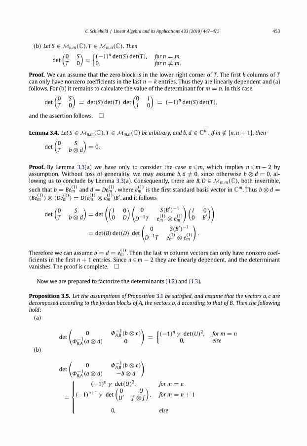
Now we are prepared to factorize the determinants (1.2) and (1.3).
Proposition 3.5. Let the assumptions of Proposition 3.1 be satisfied, and assume that the vectors a, c are
decomposed according to the Jordan blocks of A, the vectors b, d according to that of B. Then the following
hold:(a)
det
(0 Φ
−1A,B (b ⊗ c)
Φ−1B,A (a ⊗ d) 0
)=(−1)n γ det(U)2, for m = n
0, else
(b)
det
(0 Φ
−1A,B (b ⊗ c)
Φ−1B,A (a ⊗ d) −b ⊗ d
)
=
⎧⎪⎪⎪⎪⎨⎪⎪⎪⎪⎩(−1)n γ det(U)2, for m = n
(−1)n+1 γ det
(0 −U
U′ f ⊗ f
), for m = n + 1
0, else
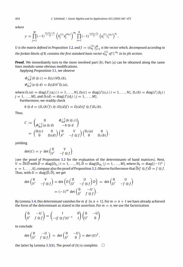
454 C. Schiebold / Linear Algebra and its Applications 433 (2010) 447–475
where
γ =M∏j=1
(−1)mj(mj+3)
2
(b(1)j d
(mj)
j
)mj N∏i=1
(−1)ni(ni+3)
2
(a(1)i c
(ni)i
)ni,
U is the matrix defined in Proposition 3.2, and f = (e(1)mj )
Mj=1 is the vector which, decomposed according to
the Jordan blocks of B, contains the first standard basis vector e(1)mj of Cmj in its jth section.
Proof. We immediately turn to the more involved part (b). Part (a) can be obtained along the same
lines modulo some obvious modifications.
Applying Proposition 3.1, we observe
Φ−1A,B (b ⊗ c) = Dl(c)VDr(b),
Φ−1B,A (a ⊗ d) = Dl(d)V
′Dr(a),
whereDr(a) = diagΓr(ai) | i = 1, . . . , N, Dl(c) = diagΓl(ci) | i = 1, . . . , N, Dr(b) = diagΓr(bj) |j = 1, . . . , M, and Dl(d) = diagΓl(dj) | j = 1, . . . , M.
Furthermore, we readily check
b ⊗ d = (Dr(b)′f )⊗ (Dl(d)f ) = Dl(d)(f ⊗ f )Dr(b).
Thus,
C :=(
0 Φ−1A,B (b ⊗ c)
Φ−1B,A (a ⊗ d) −b ⊗ d
)
=(Dl(c) 0
0 Dl(d)
)(0 V
V ′ −f ⊗ f
)(Dr(a) 0
0 Dr(b)
),
yielding
det(C) = γ det
(0 V
V ′ −f ⊗ f
)(see the proof of Proposition 3.2 for the evaluation of the determinants of band matrices). Next,
V = DUDwith D = diagDni | i = 1, . . . , N, D = diagDmj| j = 1, . . . , M, whereDk = diag(−1)κ |
κ = 1, . . . , k, compare also theproof of Proposition3.2.Observe furthermore that D(f ⊗ f )D = f ⊗ f .
Thus, with D = diagD, D, we get
det
(0 V
V ′ −f ⊗ f
)= det
(D
(0 U
U′ −f ⊗ f
)D
)= det
(0 U
U′ −f ⊗ f
)= (−1)m det
(0 −U
U′ f ⊗ f
).
By Lemma 3.4, this determinant vanishes form /∈ n, n + 1. Form = n + 1we have already achieved
the form of the determinant as stated in the assertion. Form = n, we use the factorization(0 −U
U′ f ⊗ f
)=(
I 0
−(f ⊗ f )U−1 I
)(0 −U
U′ 0
)
to conclude
det
(0 −U
U′ f ⊗ f
)= det
(0 −U
U′ 0
)= det (U)2 ,
the latter by Lemma 3.3(b). The proof of (b) is complete.

C. Schiebold / Linear Algebra and its Applications 433 (2010) 447–475 455
4. Extension of a result of Cauchy
In this section we complete the calculation of the determinant (1.1). The main step is the following
theorem.
Theorem 4.1. Assume that αi, i = 1, . . . , N, and βj , j = 1, . . . , M, are complex numbers satisfying αi +βj /= 0 for all i, j. Let ni, i = 1, . . . , N, and mj, j = 1, . . . , M, be natural numbers such that
∑Ni=1 ni =∑M
j=1 mj = n.
Then the determinant of the matrix U = (Uij) i=1,...,Nj=1,...,M
∈ Mn,n(C) with the blocks
Uij =⎛⎝( 1
αi + βj
)ν+μ−1 (ν + μ− 2
ν − 1
)⎞⎠ν=1,...,niμ=1,...,mj
∈ Mni,mj(C)
has the following value:
det(U) =N∏i<ji,j=1
(αi − αj)ninj
M∏i<ji,j=1
(βi − βj)mimj
/ N∏i=1
M∏j=1
(αi + βj)nimj .
In the simplest case (nj = mj = 1) the result was already known to Cauchy ([6, pp. 151–159]), see also
Lemma 4.2. The proof of the general case has been presented in the author’s habilitation thesis [23].
To start with, we introduce the following notation. In our calculations, the first row/column often
has to be treated separately. In this case we write
det(Tij)
i=1,...,Nj=1,...,M
= det
(T11 T1jTi1 Tij
)i>1j>1
.
Before we enter the proof, we discuss two special cases, each of them requiring a strategy of its own.
In the proof of Theorem 4.1 we will combine both strategies skilfully.
First we review Cauchy’s result, i.e. the case of one-dimensional blocks, nj = mj = 1 for
j = 1, . . . , N. We follow the proof from [18], but modify the arguments slightly to adapt it to the
proof of Theorem 4.1.
Lemma 4.2. Let αi,βj ∈ C, i, j = 1, . . . , N, with αi + βj /= 0 ∀i, j. Then
det
(1
αi + βj
)Ni,j=1
=N∏
i=1
1
(αi + βi)
N∏i,j=1i<j
(αi − αj)(βi − βj)
(αi + βj)(αj + βi).
Proof. We pursue the following strategy:
(1) (Manipulations with respect to rows) Subtract the first row from the ith row for i = 2, . . . , N.
(2) (Manipulations with respect to columns)Multiply the first columnwith (α1 + β1)/(α1 + βj) andthen subtract it from the jth column for j = 2, . . . , N.
This yields
:= det
(1
αi + βj
)Ni,j=1
(1)= det
⎛⎝ 1α1+βj[
1αi+βj − 1
α1+βj]⎞⎠
i>1j 1
= det
⎛⎝ 1α1+βj
1αi+βj
α1−αiα1+βj
⎞⎠i>1j 1

456 C. Schiebold / Linear Algebra and its Applications 433 (2010) 447–475
(2)= det
⎛⎝ 1α1+β1 0
1α1+β1
α1−αiαi+β1
[1
αi+βj − 1αi+β1
]α1−αiα1+βj
⎞⎠i>1j>1
= det
⎛⎝ 1α1+β1 0
1α1+β1
[α1−αiαi+β1
]1
αi+βj[β1−βjα1+βj
] [α1−αiαi+β1
]⎞⎠i>1j>1
.
Next we extract the common factors (β1 − βj)/(α1 + βj) from the jth column (j = 2, . . . , N) and(α1 − αi)/(αi + β1) from the ith row (i = 2, . . . , N). Finally, expanding the determinantwith respect
to the first column, we obtain
= 1
α1 + β1
∏1<j
(α1 − αj)(β1 − βj)
(αj + β1)(α1 + βj)det
(1
αi + βj
)Ni,j=2
,
and the assertion follows by induction.
Next we consider the case that T only consists of a single block, i.e., M = N = 1.
Lemma 4.3. For γ ∈ C, it holds
det
(γ ν+μ−1
(ν + μ− 2
ν − 1
))nν ,μ=1
= γ n2 .
Proof. With special regard to the order induced by the numbering of the indices, we pursue the
following strategy:
(1) (Manipulations with respect to columns)Multiply the (μ− 1)th column by γ and subtract it from
the μth column for μ = n, . . . , 2.(2) (Manipulations with respect to rows) Multiply the (ν − 1)th row by γ and subtract it from the
νth row for ν = n, . . . , 2.
This results in
:= det
(γ ν+μ−1
(ν + μ− 2
ν − 1
))nν ,μ=1
(1)= det
(γ ν γ ν+μ−1
[(ν + μ− 2
ν − 1
)−(ν + μ− 3
ν − 1
)])ν 1μ>1
= det
⎛⎝ γ 0
γ ν γ ν+μ−1
(ν + μ− 3
ν − 2
)⎞⎠ν>1μ>1
(2)= det
⎛⎜⎜⎝γ 0
0 γ μ+1 [1 − 0]
0 γ ν+μ−1
[(ν + μ− 3
ν − 2
)−(ν + μ− 4
ν − 3
)]⎞⎟⎟⎠
ν>2μ 2
= det
⎛⎝γ 0
0 γ 2·γ ν+μ−3
(ν + μ− 4
ν − 2
)⎞⎠ν>1μ>1
.
Next we expand the determinant, and then extract the factor γ 2, which all the remaining rows and
columns have in common. We end up with

C. Schiebold / Linear Algebra and its Applications 433 (2010) 447–475 457
= γ ·γ 2(n−1) det
(γ ν+μ−1
(ν + μ− 2
ν − 1
))n−1
ν ,μ=1
,
and the assertion again follows by induction.
Wenowturn to theproof of Theorem4.1. Its key idea consists in a combinationof theproof strategies
developed in Lemmas 4.2 and 4.3.
ProofofTheorem4.1. It suffices toconsider thesituationwhereαi /= αj forall i, j = 1, . . . , N, i /= j, and
βi /= βj for all i, j = 1, . . . , M, i /= j, since otherwise the matrix U would contain linearly dependent
rows or columns.
Our aim is to argue by induction. To keep the manipulations as clear as possible, we replace the
usual operations of columns/rows by the multiplication with corresponding matrices.
We use the following notations. By Uij we denote the ijth block of U, and for its entries we write
Uij =⎛⎝( 1
αi + βj
)ν+μ−1
u[i, j]νμ⎞⎠
ν=1,...,niμ=1,...,mj
. (4.1)
In the proof we will construct matrices U〈k〉 with blocks U〈k〉ij . The numbers u[i, j]〈k〉νμ will be related to
the entries of U〈k〉ij exactly as in (4.1).
Moreover, we define
Φi = α1 − αi
αi + β1, φij = α1 − αi
α1 + βj, Ψj = β1 − βj
α1 + βj, and ψji = β1 − βj
αi + β1(4.2)
for i = 1, . . . , N, j = 1, . . . , M. Note in particular, φ1j = 0 andψ1i = 0 (∀i, j).
Claim 4.4. det(U) = det(U〈1〉), where the blocks U〈1〉ij of U〈1〉 for i = 1, . . . , N, j = 1, . . . , M are given
by (u[i, j]〈1〉νμ
)ν=1,...,niμ=1,...,mj
=⎛⎝ 1 φij
ψji
(ν + μ− 4
ν − 1
)φij +
(ν + μ− 4
μ− 1
)ψji +
(ν + μ− 4
ν − 2
) [1 + φijψji
]⎞⎠ν>1μ>1
.
In particular,
U〈1〉1j =
(1
α1+βj 0
∗ ∗)ν>1μ>1
and U〈1〉i1 =
(1
αi+β1 ∗0 ∗
)ν>1μ>1
.
Proof of Claim 4.4 (Arguments within the single blocks). Here we use the strategy developed in Lemma
4.3 to create zero entries in the first column of the blocks Ui1, i = 1, . . . , N, and in the first row of the
blocks U1j , j = 1, . . . , M.
To this end, define
Xi =
⎛⎜⎜⎜⎜⎝1 0
xi ·· ·
· ·0 xi 1
⎞⎟⎟⎟⎟⎠ ∈ Mni,ni(C), Yj =
⎛⎜⎜⎜⎜⎝1 0
yj ·· ·
· ·0 yj 1
⎞⎟⎟⎟⎟⎠ ∈ Mmj,mj(C),
with xi = − 1αi+β1 , yj = − 1
α1+βj for i = 1, . . . , N and j = 1, . . . , M.
Since the det(Xi) = det(Yj) = 1 ∀i, j, the following manipulation does not change the value of the
determinant of U:

458 C. Schiebold / Linear Algebra and its Applications 433 (2010) 447–475
det(U) = det(diagX1, . . . , XN U diagY ′
1, . . . , Y′M)
= det
((XiUijY
′j
)i=1,...,Nj=1,...,M
).
It remains to explicitly calculate the entries ofU〈1〉ij = XiUijY
′j ∈ Mni,mj
(C), wherewe use the notation
introduced in the beginning of the proof, compare (4.1). We compute(1
αi + βj
)ν+μ−1
u[i, j]〈1〉νμ =(
1
αi + βj
)ν+μ−1
u[i, j]νμ
+ (1 − δ1μ) yj
(1
αi + βj
)ν+μ−2
u[i, j]ν(μ−1)
+ (1 − δ1ν) xi
(1
αi + βj
)ν+μ−2
u[i, j](ν−1)μ
+ (1 − δ1μ)(1 − δ1ν) yjxi
(1
αi + βj
)ν+μ−3
u[i, j](ν−1)(μ−1).
Therefore,
u[i, j]〈1〉νμ = u[i, j]νμ − (1 − δ1μ)αi + βj
α1 + βju[i, j]ν(μ−1) − (1 − δ1ν)
αi + βj
αi + β1u[i, j](ν−1)μ
+ (1 − δ1μ)(1 − δ1ν)αi + βj
α1 + βj
αi + βj
αi + β1u[i, j](ν−1)(μ−1)
(4.2)= u[i, j]νμ − (1 − δ1μ)[1 − φij
]u[i, j]ν(μ−1)
− (1 − δ1ν)[1 − ψji
]u[i, j](ν−1)μ
+ (1 − δ1μ)(1 − δ1ν)[1 − φij
] [1 − ψji
]u[i, j](ν−1)(μ−1).
Since u[i, j]νμ =(ν + μ− 2
ν − 1
), we immediately find
u[i, j]〈1〉νμ =⎧⎨⎩
1, ν = 1, μ = 1,
φij , ν = 1, μ > 1,
ψji, ν > 1, μ = 1,
and as for ν > 1, μ > 1, we finally calculate
u[i, j]〈1〉ν ,μ =(ν + μ− 2
ν − 1
)− (1 − φij)
(ν + μ− 3
ν − 1
)− (1 − ψji)
(ν + μ− 3
ν − 2
)+ (1 − φij)(1 − ψji)
(ν + μ− 4
ν − 2
)= φij
(ν + μ− 3
ν − 1
)+ ψji
(ν + μ− 3
ν − 2
)+ (1 − φij)(1 − ψji)
(ν + μ− 4
ν − 2
)= φij
((ν + μ− 3
ν − 1
)−(ν + μ− 4
ν − 2
))+ ψji
((ν + μ− 3
ν − 2
)−(ν + μ− 4
ν − 2
))+ (1 + φijψji)
(ν + μ− 4
ν − 2
)= φij
(ν + μ− 4
ν − 1
)+ ψji
((ν + μ− 3
μ− 1
)−(ν + μ− 4
μ− 2
))

C. Schiebold / Linear Algebra and its Applications 433 (2010) 447–475 459
+ (1 + φijψji)
(ν + μ− 4
ν − 2
)= φij
(ν + μ− 4
ν − 1
)+ ψji
(ν + μ− 4
μ− 1
)+ (1 + φijψji)
(ν + μ− 4
ν − 2
).
This completes the proof of Claim 4.4.
Claim 4.5. det(U〈1〉) = det(U〈2〉), where the blocks U〈2〉ij of U〈2〉 for i = 1, . . . , N, j = 1, . . . , M are given
by
u[1, j]〈2〉11 =1, j = 1,
0, j > 1,u[i, j]〈2〉11 =
φi1, j = 1,
φijψji, j > 1,for i > 1,
and u[i, j]〈2〉νμ = u[i, j]〈1〉νμ whenever (ν ,μ) /= (1, 1). In other words, in each block U〈1〉ij we do only change
the (1, 1)-entry.
In particular,
U〈2〉11 =
(1
α1+β1 ∗0 ∗
)ν>1μ>1
and U〈2〉1j =
(0 0
∗ ∗)ν>1μ>1
for j > 1.
Proof of Claim 4.5 (Arguments between the single blocks). The idea is to apply the strategy explained
in Lemma 4.2 with respect to the (1, 1)-entries of all blocks.
Recall that we denote by e(1)k the first standard basis vector in Ck . Define the matrices
Xi = −e(1)n1⊗ e(1)ni
∈ Mni,n1(C), Yj = −yj e(1)m1
⊗ e(1)mj∈ Mmj,m1
(C),
with yj = α1+β1α1+βj for i = 2, . . . , N, j = 2, . . . , M. Thus
U〈2〉 :=
⎛⎜⎜⎜⎝I 0 · · · 0
X2 I 0...
. . .
XN 0 I
⎞⎟⎟⎟⎠ U〈1〉
⎛⎜⎜⎜⎜⎝I Y ′
2 · · · Y ′M
0 I 0
. . .
0 0 I
⎞⎟⎟⎟⎟⎠ .
has the same determinant as U〈1〉. ObserveU
〈2〉ij = U
〈1〉ij + (1 − δ1i)XiU
〈1〉1j + (1 − δ1j)U
〈1〉i1 Y ′
j + (1 − δ1i)(1 − δ1j)XiU〈1〉11 Y ′
j
for i = 1, . . . , N, j = 1, . . . , M.
Concretely this means that we subtract the first row from the first rows of the horizontal strips
(U〈1〉i1 , . . . , U
〈1〉iM ), i = 2, . . . , N, and the (modified) first column from the first columns of the vertical
strips (U〈1〉1j , . . . , U
〈1〉Nj )
′, 2 = 1, . . . , M.
Exploiting the concrete form of U〈1〉1j (∀j) and U
〈1〉i1 (∀i) as given by Claim 4.4, we directly verify
XiU〈1〉1j = −
((U
〈1〉1j
)′e(1)n1
)⊗ e(1)ni
= − 1
α1 + βje(1)mj
⊗ e(1)ni,
and, analogously,
U〈1〉i1 Y ′
j = −yj1
αi + β1e(1)mj
⊗ e(1)ni, XiU
〈1〉11 Y ′
j = yj1
α1 + β1e(1)mj
⊗ e(1)ni.
From the fact that the matrices e(1)mj ⊗ e
(1)ni ∈ Mni,mj
(C) are zero except of the (1, 1)-entry, it is clear
that the performedmanipulation does only change the (1, 1)-entries ofU〈1〉ij , in otherwords u[i, j]〈2〉νμ =
u[i, j]〈1〉νμ whenever (ν ,μ) /= (1, 1).

460 C. Schiebold / Linear Algebra and its Applications 433 (2010) 447–475
As for the (1, 1)-entries we get
1
αi + βju[i, j]〈2〉11 = 1
αi + βj− (1 − δ1i)
1
α1 + βj− (1 − δ1j)yj
1
αi + β1
+ (1 − δ1i)(1 − δ1j)yj1
α1 + β1,
yielding
u[i, j]〈2〉11 = 1 − (1 − δ1i)αi + βj
α1 + βj− (1 − δ1j)
αi + βj
αi + β1
α1 + β1
α1 + βj
+ (1 − δ1i)(1 − δ1j)αi + βj
α1 + βj
= 1 − (1 − δ1j)α1 + β1
αi + β1
αi + βj
α1 + βj− δ1j(1 − δ1i)
αi + β1
α1 + β1
(we may replace βj by β1 because of the Kronecker symbol)
(4.2)= 1 − (1 − δ1j)[1 − φijψji
]− δ1j(1 − δ1i) [1 − φi1]
Thus it is straightforward to check
u[i, 1]〈2〉11 =
1, i = 1,
φi1, i > 1,and u[i, j]〈2〉11 = φijψji for j > 1.
Sinceψ1i = 0 for all i, this completes the proof of Claim 4.5.
Claim 4.6. det(U〈2〉) =(
1α1+β1
)n1+m1−1det(U〈3〉),where theblocksU
〈3〉ij ofU〈3〉 for i = 1, . . . , N, j =
1, . . . , M are given by(u[1, 1]〈3〉νμ
)ν=1,...,n1μ=1,...,m1
=((ν + μ− 2
ν − 1
))ν 1μ 1
,
(u[i, 1]〈3〉νμ
)ν=1,...,niμ=1,...,m1
=⎛⎜⎝Φi(ν + μ− 3
ν − 2
)+(ν + μ− 2
ν − 1
)Φi
⎞⎟⎠ν>1μ 1
, for i > 1,
(u[1, j]〈3〉νμ
)ν=1,...,n1μ=1,...,mj
=(Ψj
(ν + μ− 3
ν − 1
)+(ν + μ− 2
μ− 1
)Ψj
)ν 1μ>1
, for j > 1,
(u[i, j]〈3〉νμ
)ν=1,...,niμ=1,...,mj
=⎛⎜⎝φijψji φij
ψji
(ν + μ− 4
ν − 1
)φij +
(ν + μ− 4
μ− 1
)ψji +
(ν + μ− 4
ν − 2
) [1 + φijψji
]⎞⎟⎠ν>1μ>1
,
for i > 1, j > 1.
Thenewdimensions are definedby n1 = n1 − 1 and ni = ni for i = 2, . . . , N, aswell as m1 = m1 − 1 and
mj = mj for j = 2, . . . , M. For simplicity, we consider matrices of the types 0 × k, k × 0 as non-existent.
Note that U〈3〉 ∈ Mn−1,n−1(C).

C. Schiebold / Linear Algebra and its Applications 433 (2010) 447–475 461
Proof of Claim 4.6 (Expansion of the determinant). As a preparation, we simplify the results observed
so far. To this end, abbreviate γ = (α1 + β1)−1.
Recall thatU〈2〉11 = U
〈1〉11 . SinceU
〈1〉11 was obtained by the samemodifications as in the proof of Lemma
4.3, its coefficients are as described there (see (4.4)).
As for the entries of U〈2〉1j , j > 1, we rewriteψj1 = (α1 + βj)γΨj (recall φ1j = 0), to see
u[1, j]〈2〉ν1 = (α1 + βj)γΨj (∀ν > 1),
u[1, j]〈2〉νμ =(ν + μ− 4
ν − 2
)+(ν + μ− 4
μ− 1
)(α1 + βj)γΨj
(4.3)= (α1 + βj)γ
((ν + μ− 4
ν − 2
)(1 + Ψj)+
(ν + μ− 4
μ− 1
)Ψj
)
= (α1 + βj)γ
((ν + μ− 4
ν − 2
)+(ν + μ− 3
μ− 1
)Ψj
)(∀μ > 1, ∀ν > 1).
As for the entries of U〈2〉i1 , i > 1, inserting φi1 = (αi + β1)γΦi (recall also ψ1i = 0) we analogously
get
u[i, 1]〈2〉1μ = (αi + β1)γΦi (∀μ),u[i, 1]〈2〉νμ =
(ν + μ− 4
ν − 2
)+(ν + μ− 4
ν − 1
)(αi + β1)γΦi
(4.3)= (αi + β1)γ
((ν + μ− 4
ν − 2
)(1 + Φi)+
(ν + μ− 4
ν − 1
)Φi
)= (αi + β1)γ
((ν + μ− 4
ν − 2
)+(ν + μ− 3
ν − 1
)Φi
)(∀μ > 1, ∀ν > 1).
Above we have used the identities
1
α1 + βjγ−1 = 1 + Ψj ,
1
αi + β1γ−1 = 1 + Φi. (4.3)
There is no need to consider U〈2〉ij for i > 1, j > 1, since these blocks are not altered by the expansion
below.
Let us sum up what we have achieved so far:
U〈2〉11 =
⎛⎝γ 0
0 γ 2(
1α1+β1
)ν+μ−3(ν + μ− 4
ν − 2
)⎞⎠ν>1μ>1
, (4.4)
U〈2〉1j
=⎛⎝ 0 0
γ(
1α1+βj
)ν−1Ψj γ
(1
α1+βj)ν+μ−2
((ν + μ− 4
ν − 2
)+(ν + μ− 3
μ− 1
)Ψj
)⎞⎠ν>1μ>1
, j > 1,
U〈2〉i1 =
⎛⎜⎝γΦi γ(
1αi+β1
)μ−1Φi
0 γ(
1αi+β1
)ν+μ−2((ν + μ− 4
ν − 2
)+(ν + μ− 3
ν − 1
)Φi
)⎞⎟⎠ν>1μ>1
, i > 1.
Note that, in the first row of U〈2〉, only the first entry is non-zero. Hence expanding reduces the
dimension by one, and Claim 4.6 then follows by extracting the factor γ which is common to

462 C. Schiebold / Linear Algebra and its Applications 433 (2010) 447–475
(a) the νth row, ν = 2, . . . , n1, of the blocks U〈2〉1j (∀j),
(b) the μth columns, μ = 2, . . . , m1, of the blocks U〈2〉i1 (∀i).
Claim 4.7. det(U〈3〉) =(∏N
i=2Φnii
∏Mj=2Ψ
mj
j
)det(U), where the blocks Uij of U for i = 1, . . . , N, j =
1, . . . , M are given by
Uij =⎛⎝( 1
αi + βj
)ν+μ−1 (ν + μ− 2
ν − 1
)⎞⎠ν=1,...,niμ=1,...,mj
∈ Mni ,mj(C)
and ni, mj are defined as in Claim 4.6.
Note that U is a matrix of the same form as U but of smaller size.
Proof of Claim 4.7 (Reestablishing the original structure). For i = 2, . . . , N and j = 2, . . . , M we define
the matrices
Xi = (x[i]νμ)niν ,μ=1∈ Mni ,ni(C) with x[i]νμ =
0, μ > ν ,
xν−μi , μ ν ,
Yj = (y[j]νμ)mj
ν ,μ=1 ∈ Mmj ,mj(C) with y[j]νμ =
0, μ > ν ,
yν−μj , μ ν ,
where xi = − 1αi+β1Φ
−1i , yj = − 1
α1+βjΨ−1j . Again det(Xi) = det(Yj) = 1, and thus
U〈4〉 := diagI, X2, . . . , XN U〈3〉 diagI, Y ′2, . . . , Y
′M
=⎛⎜⎝ U
〈3〉11 U
〈3〉1j Y ′
j
XiU〈3〉i1 XiU
〈3〉ij Y ′
j
⎞⎟⎠i>1j>1
has the same determinant as U〈3〉.Note that U〈4〉 has the blocks U
〈4〉ij = XiU
〈3〉ij Y ′
j , where, for the sake of convenience, we adopt the
convention X1 = I ∈ Mn1 ,n1(C) and Y1 = I ∈ Mm1 ,m1(C).
Calculating the entries of U〈4〉ij we get(
1
αi + βj
)ν+μ−1
u[i, j]〈4〉νμ
=ν∑λ=1
μ∑κ=1
(1
αi + βj
)λ+κ−1
xν−λi u[i, j]〈3〉λκ y
μ−κj
=(
1
αi + βj
)ν+μ−1 ν∑λ=1
μ∑κ=1
((αi + βj)xi
)ν−λ ((αi + βj)yj
)μ−κu[i, j]〈3〉λκ .
With pij :=(αi + βj)xi and qij := (αi + βj)yj , the above identity rewrites as
u[i, j]〈4〉νμ =ν∑λ=1
μ∑κ=1
pν−λij q
μ−κij u[i, j]〈3〉λκ , (4.5)
where, for later use, we note

C. Schiebold / Linear Algebra and its Applications 433 (2010) 447–475 463
pij =⎧⎪⎨⎪⎩0, i = 1, j 1,
−Φ−1i , i > 1, j = 1,
1 − φ−1ij , i > 1, j > 1,
qij =⎧⎪⎨⎪⎩0, j = 1, i 1,
−Ψ−1j , j > 1, i = 1,
1 − ψ−1ji , j > 1, i > 1.
(4.6)
To evaluate (4.5), the following simple identity is helpful. For γ ∈ C and S, R ∈ N,
R∑r=2
γ R−r
[(S + r − 3
S − 1
)− γ−1
(S + r − 2
S − 1
)]= γ R−2 − γ−1
(S + R − 2
S − 1
). (4.7)
We start with the calculation of (4.5) in the case i = 1, j > 1. Since p1j = 0, Ψj = −q−11j for j > 1 by
(4.6), we observe
u[1, j]〈4〉νμ =μ∑κ=1
qμ−κ1j u[1, j]〈3〉νκ
= qμ−11j Ψj +
μ∑κ=2
qμ−κ1j
[(ν + κ − 3
ν − 1
)+(ν + κ − 2
μ− 1
)Ψj
]
= −qμ−21j +
μ∑κ=2
qμ−κ1j
[(ν + κ − 3
ν − 1
)− q
−11j
(ν + κ − 2
ν − 1
)](4.7)= −q
−11j
(ν + μ− 2
ν − 1
)= Ψj
(ν + μ− 2
ν − 1
).
Analogously, in the case i > 1, j = 1 we get u[i, 1]〈4〉νμ = Φi
(ν + μ− 2
ν − 1
).
The case i > 1, j > 1 is slightlymore involved. Hereφij = (1 − pij)−1 andψji = (1 − qij)
−1, again
by (4.6). Thus the entries u[i, j]〈3〉λκ we start from are given by
u[i, j]〈3〉11 = φijψji = ((1 − pij)(1 − qij)
)−1,
u[i, j]〈3〉λ1 = ψji = ((1 − pij)(1 − qij))−1 ·(1 − pij), λ > 1,
u[i, j]〈3〉1κ = φij = ((1 − pij)(1 − qij))−1 ·(1 − qij), κ > 1,
u[i, j]〈3〉λκ =(λ+ κ − 4
λ− 1
)φij +
(λ+ κ − 4
κ − 1
)ψji +
(λ+ κ − 4
λ− 2
) [1 + φijψji
]= ((1 − pij)(1 − qij)
)−1[(λ+ κ − 2
λ− 1
)− qij
(λ+ κ − 3
λ− 1
)− pij
(λ+ κ − 3
λ− 2
)+ pijqij
(λ+ κ − 4
λ− 2
)], λ > 1, κ > 1,
the latter by the usual properties of binomial coefficients. Let μ > 1, ν > 1. Exploiting these repre-
sentations, we obtain
(1 − pij)(1 − qij)
μ∑κ=2
qμ−κij u[i, j]〈3〉λκ
= −qij
μ∑κ=2
qμ−κij
[(λ+ κ − 3
λ− 1
)− q
−1ij
(λ+ κ − 2
λ− 1
)]
+ pijqij
μ∑κ=2
qμ−κij
[(λ+ κ − 4
λ− 2
)− q
−1ij
(λ+ κ − 3
λ− 2
)]

464 C. Schiebold / Linear Algebra and its Applications 433 (2010) 447–475
(4.7)= −qij
(qμ−2ij − q
−1ij
(λ+ μ− 2
λ− 1
))+ pijqij
(qμ−2ij − q
−1ij
(λ+ μ− 3
λ− 2
))
=[(λ+ μ− 2
λ− 1
)− pij
(λ+ μ− 3
λ− 2
)]− q
μ−1ij (1 − pij)
=[(λ+ μ− 2
μ− 1
)− pij
(λ+ μ− 3
μ− 1
)]− q
μ−1ij (1 − pij), if λ > 1.
Hence,
(1 − pij)(1 − qij)ν∑λ=2
μ∑κ=2
pν−λij q
μ−κij u[i, j]〈3〉λκ
= −pij
ν∑λ=2
pν−λij
[(λ+ μ− 3
μ− 1
)− p
−1ij
(λ+ μ− 2
μ− 1
)]+ pijq
μ−1ij
ν∑λ=2
pν−λij (1 − p
−1ij )
(4.7)= −pij
(pν−2ij − p
−1ij
(ν + μ− 2
μ− 1
))+ pijq
μ−1ij
(pν−2ij − p
−1ij
)
=(ν + μ− 2
μ− 1
)+ (1 − p
ν−1ij )(1 − q
μ−1ij )− 1. (4.8)
In addition, we verify that
(1 − pij)(1 − qij)
⎛⎝pν−1ij q
μ−1ij u[i, j]〈3〉11 + q
μ−1ij
ν∑λ=2
pν−λij u[i, j]〈3〉λ1 + p
ν−1ij
μ∑κ=2
qμ−κij u[i, j]〈3〉1κ
⎞⎠= p
ν−1ij q
μ−1ij + q
μ−1ij
ν∑λ=2
pν−λij (1 − pij)+ p
ν−1ij
μ∑κ=2
qμ−κij (1 − qij)
= −(1 − pν−1ij )(1 − q
μ−1ij )+ 1. (4.9)
Consequently, inserting (4.8), (4.9) into (4.5) yields (1 − pij)(1 − qij) u[i, j]〈4〉λκ =(ν + μ− 2
ν − 1
), which
by (4.2), (4.6) finally shows
u[i, j]〈4〉λκ = φijψji
(ν + μ− 2
ν − 1
)= ΦiΨj
(ν + μ− 2
ν − 1
).
To sum up,
U〈4〉11 = U11,
U〈4〉i1 = ΦiUi1, i > 1,
U〈4〉1j = ΨjU1j , j > 1,
U〈4〉ij = ΦiΨjUij , i > 1, j > 1,
and Claim 4.7 follows by extracting common factors.
Induction with respect to the dimension n: We conclude by carrying out the induction argument.
To this end, assume that the assertion holds for all dimensions less then n. By Claims 4.4–4.7,
det(U) =[
1
α1 + β1
]n1+m1−1 N∏i=2
[α1 − αi
αi + β1
]ni M∏j=2
[β1 − βj
α1 + βj
]mj
det(U), (4.10)
where U ∈ Mn−1,n−1(C) is precisely of the same structure as U. Thus, by the assumption of the
induction,

C. Schiebold / Linear Algebra and its Applications 433 (2010) 447–475 465
det(U) =N∏
i,j=1i<j
(αi − αj)ni nj
M∏i,j=1i<j
(βi − βj)mimj
/ N∏i=1
M∏j=1
(αi + βj)nimj
=
[1
α1 + β1
](n1−1)(m1−1) N∏i=2
[(α1 − αi)
n1−1
(αi + β1)m1−1
]ni M∏j=2
[(β1 − βj)
m1−1
(α1 + βj)n1−1
]mj
(4.11)
for =N∏
i,j=2i<j
(αi − αj)ninj
M∏i,j=2i<j
(βi − βj)mimj
/ N∏i=2
M∏j=2
(αi + βj)nimj .
Inserting (4.11) into (4.10) immediately yields the desired formula for det(U).This completes the proof of Theorem 4.1. Combining Proposition 3.2 and Theorem 4.1, we finally obtain
Theorem 4.8. LetA, B ∈ Mn,n(C)be in Jordan canonical formwith JordanblocksAi, Bj of dimensionsni, mj
corresponding to eigenvalues αi,βj , respectively. Assume αi + βj /= 0 for all i = 1, . . . , N, j = 1, . . . , M.Then
det(Φ
−1A,B (a ⊗ c)
)= γ
N∏i<ji,j=1
(αi − αj)ninj
M∏i<ji,j=1
(βi − βj)mimj
/ N∏i=1
M∏j=1
(αi + βj)nimj ,
where
γ = (−1)nM∏j=1
(−1)mj(mj+1)
2
(a(1)j
)mjN∏
i=1
(c(ni)i
)niwith the vectors a, c ∈ Cn decomposed according to the Jordan blocks of A, B, respectively, namely c =(ci)
Ni=1, ci =
(c(1)i , . . . , c
(ni)i
)′and a = (aj)
Mj=1, aj =
(a(1)j , . . . , a
(mj)
j
)′.
5. A further extension to determinants of double size with a one-dimensional perturbation
In this section we complete the calculation of the determinants (1.2) and (1.3). The main step is the
following theorem.
Theorem 5.1. Assume that αi, i = 1, . . . , N, and βj , j = 1, . . . , M, are complex numbers with the prop-
erty αi + βj /= 0 for all i, j. Let ni, i = 1, . . . , N, and mj, j = 1, . . . , M, be natural numbers, and set n =∑Ni=1 ni, m = ∑M
j=1 mj.
Define the matrix U = (Uij) i=1,...,Nj=1,...,M
∈ Mn,m(C) with the blocks
Uij =⎛⎝( 1
αi + βj
)ν+μ−1 (ν + μ− 2
ν − 1
)⎞⎠ν=1,...,niμ=1,...,mj
∈ Mni,mj(C)
and the vector f = (e(1)mj )
Mj=1 ∈ Cm consisting of the first standard basis vectors e
(1)mj ∈ Cmj for
j = 1, . . . , M.Then
det
(0 −U
U′ f⊗f
)=
⎧⎪⎪⎪⎪⎨⎪⎪⎪⎪⎩N∏
i,j=1i<j
(αi − αj)2ninj
M∏i,j=1i<j
(βi − βj)2mimj
/N∏
i=1
M∏j=1
(αi + βj)2nimj ,
for m ∈ n, n + 1,0, else.
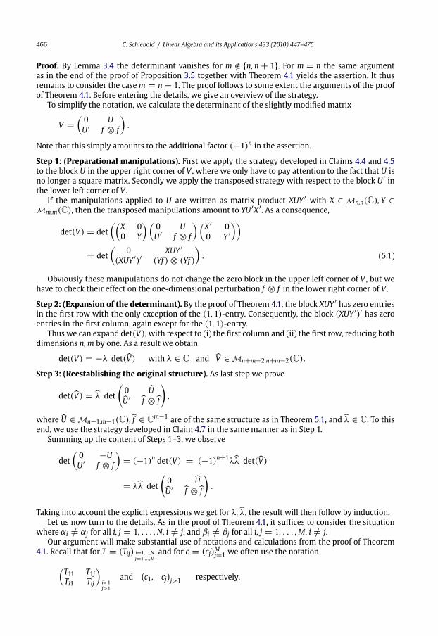
466 C. Schiebold / Linear Algebra and its Applications 433 (2010) 447–475
Proof. By Lemma 3.4 the determinant vanishes for m /∈ n, n + 1. For m = n the same argument
as in the end of the proof of Proposition 3.5 together with Theorem 4.1 yields the assertion. It thus
remains to consider the casem = n + 1. The proof follows to some extent the arguments of the proof
of Theorem 4.1. Before entering the details, we give an overview of the strategy.
To simplify the notation, we calculate the determinant of the slightly modified matrix
V =(0 U
U′ f ⊗ f
).
Note that this simply amounts to the additional factor (−1)n in the assertion.
Step 1: (Preparational manipulations). First we apply the strategy developed in Claims 4.4 and 4.5
to the block U in the upper right corner of V , where we only have to pay attention to the fact that U is
no longer a square matrix. Secondly we apply the transposed strategy with respect to the block U′ inthe lower left corner of V .
If the manipulations applied to U are written as matrix product XUY ′ with X ∈ Mn,n(C), Y ∈Mm,m(C), then the transposed manipulations amount to YU′X′. As a consequence,
det(V) = det
((X 0
0 Y
)(0 U
U′ f ⊗ f
)(X′ 0
0 Y ′))
= det
(0 XUY ′
(XUY ′)′ (Yf )⊗ (Yf )
). (5.1)
Obviously these manipulations do not change the zero block in the upper left corner of V , but we
have to check their effect on the one-dimensional perturbation f ⊗ f in the lower right corner of V .
Step 2: (Expansion of the determinant). By the proof of Theorem 4.1, the block XUY ′ has zero entries
in the first row with the only exception of the (1, 1)-entry. Consequently, the block (XUY ′)′ has zeroentries in the first column, again except for the (1, 1)-entry.
Thus we can expand det(V), with respect to (i) the first column and (ii) the first row, reducing both
dimensions n, m by one. As a result we obtain
det(V) = −λ det(V) with λ ∈ C and V ∈ Mn+m−2,n+m−2(C).
Step 3: (Reestablishing the original structure). As last step we prove
det(V) = λ det
(0 U
U′ f ⊗ f
),
where U ∈ Mn−1,m−1(C), f ∈ Cm−1 are of the same structure as in Theorem 5.1, and λ ∈ C. To this
end, we use the strategy developed in Claim 4.7 in the same manner as in Step 1.
Summing up the content of Steps 1–3, we observe
det
(0 −U
U′ f ⊗ f
)= (−1)n det(V) = (−1)n+1λλ det(V)
= λλ det
(0 −U
U′ f ⊗ f
).
Taking into account the explicit expressions we get for λ, λ, the result will then follow by induction.
Let us now turn to the details. As in the proof of Theorem 4.1, it suffices to consider the situation
where αi /= αj for all i, j = 1, . . . , N, i /= j, and βi /= βj for all i, j = 1, . . . , M, i /= j.
Our argument will make substantial use of notations and calculations from the proof of Theorem
4.1. Recall that for T = (Tij) i=1,...,Nj=1,...,M
and for c = (cj)Mj=1 we often use the notation(
T11 T1jTi1 Tij
)i>1j>1
and(c1, cj
)j>1
respectively,

C. Schiebold / Linear Algebra and its Applications 433 (2010) 447–475 467
if the blocks Tij ∈ Mnimj(C)with i > 1, j > 1 (or the vector cj ∈ Cmj with j > 1) are treated separately
from the others.
In the sequel we will use the notation X〈k〉i , Y
〈k〉j for the matrices Xi, Yj used in the proof of the
kth claim of Theorem 4.1. Note that their dimension depends on k, for example Y〈1〉j ∈ Mmj,mj
(C) for
j = 1, . . . , M and Y〈2〉j ∈ Mmj,m1
(C) for j = 2, . . . , M.
Similarly as in the proof of Theorem4.1,we gather the Y〈k〉j in one commonmatrix Y 〈k〉. Analogously,
the matrix X〈k〉 collects the X〈k〉j . For example,
Y 〈1〉 =
⎛⎜⎜⎜⎝Y
〈1〉1 0
. . .
0 Y〈1〉M
⎞⎟⎟⎟⎠ , Y 〈2〉 =
⎛⎜⎜⎜⎝1 0 · · · 0
Y〈2〉2 1 · · · 0
. . . . . . . . . . . . . . . . . . . . . . . . . .
Y〈2〉M 0 · · · 1
⎞⎟⎟⎟⎠ . (5.2)
Recall det(X〈k〉) = det(Y 〈k〉) = 1 for all k.
Note that the manipulations with respect to rows and columns used in the proof of Theorem 4.1
did not depend on the fact that n = m. Actually, the fact that U is a square matrix was only needed for
the existence of det(U). Hence we can be brief in the following arguments.
Step 1:With X = X〈2〉X〈1〉, Y = Y 〈2〉Y 〈1〉, we can apply (5.1), since det(X) = det(Y) = 1, and it follows
det(V) = det
(0 U〈2〉
(U〈2〉)′ f 〈2〉 ⊗ f 〈2〉),
where U〈2〉 is the matrix obtained in Claims 4.4 and 4.5, and f 〈2〉 = Yf . The key point is that, except of
the (1, 1)-entry, U〈2〉 has only zero entries in the first row. Similarly, (U〈2〉)′ has only zero entries in
the first column except of the (1, 1)-entry. The value of these (1, 1)-entries is (α1 + β1)−1.
Let us calculate f 〈2〉. With f = (fj)Mj=1, we infer by (5.2)
f 〈2〉 =(Y
〈1〉1 f1, Y
〈1〉j fj + Y
〈2〉j Y
〈1〉1 f1
)j>1.
Inserting the concrete expressions for Y〈1〉j , Y
〈2〉j , as given in the proofs of Claims 4.4 and 4.5, and
fj = e(1)mj , we get
Y〈1〉j fj = e(1)mj
− 1
α1 + βje(2)mj
, j = 1, . . . , M,
Y〈2〉j Y
〈1〉1 f1 = −α1 + β1
α1 + βje(1)mj
, j = 2, . . . , M,
where, for simplicity, we consider the κth standard basis vector e(κ)k ∈ Ck as non-existent for κ > k.
In summary,
f 〈2〉 =(e(1)m1
− 1
α1 + β1e(2)m1
,−β1 − βj
α1 + βje(1)mj
− 1
α1 + βje(2)mj
)j>1
. (5.3)
Step 2: Set γ = (α1 + β1)−1. In the proof of Claim 4.6, we have shown that the matrix U〈2〉 is of the
form
U〈2〉 =⎛⎜⎜⎝γ 0 0
∗ γ 2U〈3〉11 γU
〈3〉1j
∗ γU〈3〉i1 U
〈3〉ij
⎞⎟⎟⎠i>1j>1
,U
〈3〉1j with n1 − 1 rows (∀j),
U〈3〉i1 withm1 − 1 columns (∀i),
with U〈3〉ij as defined in Claim 4.6.
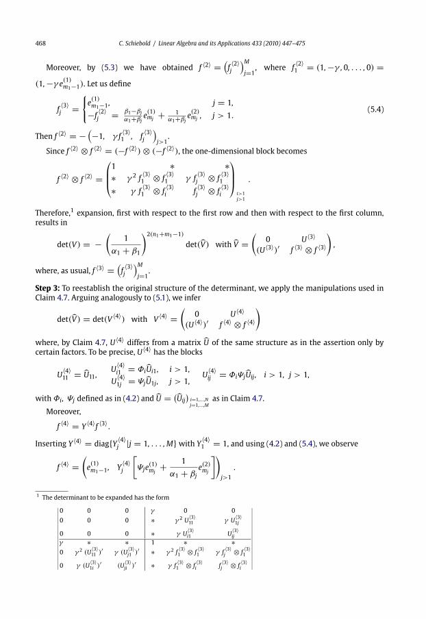
468 C. Schiebold / Linear Algebra and its Applications 433 (2010) 447–475
Moreover, by (5.3) we have obtained f 〈2〉 =(f〈2〉j
)Mj=1
, where f〈2〉1 = (1,−γ , 0, . . . , 0) =
(1,−γ e(1)m1−1). Let us define
f〈3〉j =
⎧⎨⎩e(1)m1−1, j = 1,
−f〈2〉j = β1−βj
α1+βj e(1)mj + 1
α1+βj e(2)mj , j > 1.
(5.4)
Then f 〈2〉 = −(−1, γ f
〈3〉1 , f
〈3〉j
)j>1
.
Since f 〈2〉 ⊗ f 〈2〉 = (−f 〈2〉)⊗ (−f 〈2〉), the one-dimensional block becomes
f 〈2〉 ⊗ f 〈2〉 =⎛⎜⎜⎝1 ∗ ∗∗ γ 2 f
〈3〉1 ⊗ f
〈3〉1 γ f
〈3〉j ⊗ f
〈3〉1
∗ γ f〈3〉1 ⊗ f
〈3〉i f
〈3〉j ⊗ f
〈3〉i
⎞⎟⎟⎠i>1j>1
.
Therefore,1 expansion, first with respect to the first row and then with respect to the first column,
results in
det(V) = −(
1
α1 + β1
)2(n1+m1−1)
det(V) with V =(
0 U〈3〉(U〈3〉)′ f 〈3〉 ⊗ f 〈3〉
),
where, as usual, f 〈3〉 =(f〈3〉j
)Mj=1
.
Step 3: To reestablish the original structure of the determinant, we apply the manipulations used in
Claim 4.7. Arguing analogously to (5.1), we infer
det(V) = det(V 〈4〉) with V 〈4〉 =(
0 U〈4〉(U〈4〉)′ f 〈4〉 ⊗ f 〈4〉
)
where, by Claim 4.7, U〈4〉 differs from a matrix U of the same structure as in the assertion only by
certain factors. To be precise, U〈4〉 has the blocks
U〈4〉11 = U11,
U〈4〉i1 = ΦiUi1, i > 1,
U〈4〉1j = ΨjU1j , j > 1,
U〈4〉ij = ΦiΨjUij , i > 1, j > 1,
withΦi, Ψj defined as in (4.2) and U = (Uij
)i=1,...,Nj=1,...,M
as in Claim 4.7.
Moreover,
f 〈4〉 = Y 〈4〉f 〈3〉.
Inserting Y 〈4〉 = diagY 〈4〉j |j = 1, . . . , M with Y
〈4〉1 = 1, and using (4.2) and (5.4), we observe
f 〈4〉 =(e(1)m1−1, Y
〈4〉j
[Ψje
(1)mj
+ 1
α1 + βje(2)mj
])j>1
.
1 The determinant to be expanded has the form∣∣∣∣∣∣∣∣∣∣∣∣∣∣∣∣∣
0 0 0 γ 0 0
0 0 0 ∗ γ 2 U〈3〉11 γ U
〈3〉1j
0 0 0 ∗ γ U〈3〉i1 U
〈3〉ij
γ ∗ ∗ 1 ∗ ∗0 γ 2 (U
〈3〉11 )
′ γ (U〈3〉j1 )
′ ∗ γ 2 f〈3〉1 ⊗ f
〈3〉1 γ f
〈3〉j ⊗ f
〈3〉1
0 γ (U〈3〉1i )
′ (U〈3〉ji )
′ ∗ γ f〈3〉1 ⊗ f
〈3〉i f
〈3〉j ⊗ f
〈3〉i
∣∣∣∣∣∣∣∣∣∣∣∣∣∣∣∣∣

C. Schiebold / Linear Algebra and its Applications 433 (2010) 447–475 469
As in Claim 4.7, set yj = − ((α1 + βj)Ψj
)−1. Then, from the concrete form of Y
〈4〉j , j = 2, . . . , M, in
Claim 4.7, we immediately find
Y〈4〉j
[Ψje
(1)mj
+ 1
α1 + βje(2)mj
]= Ψje
(1)mj
+mj∑μ=2
(Ψjy
mj−1
j + 1
α1 + βjymj−2
j
)e(μ)mj
= Ψje(1)mj
+ 1
α1 + βj
mj∑μ=2
(− 1
yjymj−1
j + ymj−2
j
)e(μ)mj
= Ψje(1)mj.
As a consequence,
f 〈4〉 =(e(1)m1−1,Ψje
(1)mj
)j>1
=(f1,Ψj fj
)j>1
,
if we define f1 = e(1)m1−1 and fj = e
(1)mj . In addition, set f = (fj)
Mj=1.
Therefore,2 we can extract the factor Φi from the ni rows, i = 2, . . . , N, of the blocks in the upper
right corner of S〈4〉 and the factor Ψi from the mi rows, i = 2, . . . , M, of the blocks in the lower left
corner of S〈4〉. Similarly, we extract the factor Ψj from the mj columns, j = 2, . . . , M, of the blocks in
the upper right corner of S〈4〉 and the factorΦj from the nj columns, j = 2, . . . , N, of the blocks in the
lower left corner of S〈4〉.As a result,
det(V) =N∏
i=2
Φ2nii
M∏j=2
Ψ2mj
j det
⎛⎝ 0 U
U′ f ⊗ f
⎞⎠ .Result of Step1 to Step 3: Let us sum up what we have achieved so far. Namely, starting from the
original matrix, we get
det
(0 −U
U′ f ⊗ f
)= (−1)n det(V)
Step2= (−1)n+1
[1
α1 + β1
]2(n1+m1−1)
det(V)
Step3= (−1)n+1
[1
α1 + β1
]2(n1+m1−1) N∏i=2
Φ2nii
M∏j=2
Ψ2mj
j det
(0 U
U′ f ⊗ f
)
=[
1
α1 + β1
]2(n1+m1−1) N∏i=2
Φ2nii
M∏j=2
Ψ2mj
j det
(0 −U
U′ f ⊗ f
).
2 In summary we have now observed
|V 〈4〉| =∣∣∣∣∣ 0 U〈4〉
(U〈4〉)′ f 〈4〉 ⊗ f 〈4〉
∣∣∣∣∣ =∣∣∣∣∣∣∣∣∣∣∣
0 0 U11 Ψj U1j
0 0 ΦiUi1 ΦiΨj Uij
U′11 Φj U
′j1 f1 ⊗ f1 Ψj fj ⊗ f1
ΨiU′1i ΨiΦj U
′ji Ψi f1 ⊗ fi ΨiΨj fj ⊗ fi
∣∣∣∣∣∣∣∣∣∣∣.

470 C. Schiebold / Linear Algebra and its Applications 433 (2010) 447–475
Inserting (4.2), we in summary have proved
det
(0 −U
U′ f ⊗ f
)= (5.5)
=[
1
α1 + β1
]2(n1+m1−1) N∏i=2
[α1 − αi
αi + β1
]2ni M∏j=2
[β1 − βj
α1 + βj
]2mj
det
(0 −U
U′ f ⊗ f
),
where the latter matrix is of the same structure as in the assertion, but is of lower dimension.
Induction: Comparison to the proof of Theorem 4.1 shows that the induction stepwith respect to (5.5)
can be carried over almost literally. The only difference is an additional square appearing in the factors.
This completes the proof.
Combining Proposition 3.5 and Theorem 5.1, we finally obtain
Theorem 5.2. Let A ∈ Mn,n(C) and B ∈ Mm,m(C) be in Jordan canonical form with Jordan blocks Ai, Bjof dimensions ni, mj corresponding to the eigenvalues αi,βj , respectively. Assume αi + βj /= 0 for all i =1, . . . , N, j = 1, . . . , M. Then
(a)
det
(0 Φ
−1A,B (b ⊗ c)
Φ−1B,A (a ⊗ d) 0
)=(−1)m γ u, for m = n
0, else,
(b)
det
(0 Φ
−1A,B (b ⊗ c)
Φ−1B,A (a ⊗ d) −b ⊗ d
)=(−1)m γ u, for m ∈ n, n + 1,
0, else,
where
u =N∏i<ji,j=1
(αi − αj)2ninj
M∏i<ji,j=1
(βi − βj)2mimj
/ N∏i=1
M∏j=1
(αi + βj)2nimj
and
γ =M∏j=1
(−1)mj(mj+3)
2
(b(1)j d
(mj)
j
)mj N∏i=1
(−1)ni(ni+3)
2
(a(1)i c
(ni)i
)niwith the vectors a, c ∈ Cn decomposed according to the Jordan blocks of A, the vectors b, d ∈ Cm
according to that of B, respectively, namely c = (ci)Ni=1, ci = (c
(1)i , . . . , c
(ni)i )′ and d = (dj)
Mj=1,
dj = (d(1)j , . . . , d
(mj)
j )′.
6. Applications
In the sequelwe explain how the results on Cauchy-type determinants can be used to determine the
asymptotics ofmultiple pole solutions. Since a general treatment of the class ofmultiple pole solutions
is beyond the scope of the present article, we focus here on the discussion of some accessible aspects.
For a rigorous treatment of the complete class of multiple pole solutions the reader is referred to
[20] for the KdV, [21] for the sine-Gordon equation, [22] for the Toda lattice, [23]where a simultaneous
treatment of the regular reductions of the AKNS system can be found, and the forthcoming article [27]
for the nonlinear Schrödinger equation.

C. Schiebold / Linear Algebra and its Applications 433 (2010) 447–475 471
6.1. Korteweg–de Vries equation
For illustration let us consider the case that A has two Jordan blocks A1, A2, with eigenvaluesα1, α2,and that A1 is of size 1. To fix ideas we suppose 0 < α1 < α2, the other cases being similar.
Inserting these data into (2.1), the resulting solution formula reads
u(x, t)=2∂2
∂x2log p(x, t),
where p(x, t) = det
(I +(Li(x, t)Φ
−1Ai,Aj
(aj ⊗ ci
))i,j=1,2
),
with L1 = 1, L2 = 2T , where i = i(x, t) = exp(αix + α3
i t)for i = 1, 2 and T is an upper tri-
angular matrix the diagonal entries of which are 1 and the off-diagonal entries are polynomials in
x, t.
Before proceeding we observe that the data A = (α),α /= 0, and a, c with ac = 2α (i.e. A a 1 ×1-matrix, a, c numbers) leads to the solution
sα(x, t) = 2∂2
∂x2log
(1 + ac
2αexp(αx + α3t)
)
= α2
2cosh−2
(α
2(x + α2t)
).
This is the 1-soliton, a bell-shaped solitary wave traveling with constant speed −α2. Note that for
ac = −2α we get the antisoliton
−α2
2sinh−2
(α
2(x + α2t)
),
a solitary ‘wave’ with second-order pole (see Fig. 1).
We now do an informal asymptotic analysis of the solution u(x, t). We will see that the block A1
gives rise to the solution having a soliton component. Our aim is to study the effect of the other solution
component, due to the block A2, on this soliton.
As we expect u(x, t), for large times t, to exhibit a soliton component sα1(x + δ, t) for some δ, let
us move with corresponding speed −α21 , that is let
x + α21 t = const. (6.1)
To understand the behavior of L2(x, t), for |t| large, we observe that α2x + α32 t =
const + α2(α22 − α2
1)t → ±∞ as t → ±∞.
Large negative times. If (6.1) holds and t → −∞, the entries of the matrix L2(x, t) decay rapidly, and
we get
Fig. 1. Snapshot of soliton and antisoliton solutions (α = 1) of the Korteweg–de Vries equation.

472 C. Schiebold / Linear Algebra and its Applications 433 (2010) 447–475
p(x, t) ≈ det
(I + L1(x, t) Φ
−1A1 ,A1
(a1 ⊗ c1) L1(x, t) Φ−1A1 ,A2
(a2 ⊗ c1)0 I
)= det
(I + L1(x, t) Φ
−1A1 ,A1
(a1 ⊗ c1))
= 1 + a1c1
2α11(x, t).
For simplicity we assume that u(x, t) looks like a 1-soliton (and not like an antisoliton), which means
that we suppose a1c1 > 0. Then u(x, t) ≈ sα1(x + δ−, t) with the initial position −δ− being deter-
mined by (a1c1)/(2α1) = exp(α1δ
−/2).
Large positive times. If (6.1) holds and t → ∞, the entries of the matrix L2(x, t) explode. However, it
is easy to see that those of L−12 (x, t) decay rapidly. Let
p(x, t) = det
((1 0
0 L−12
)(I +(Li(x, t)Φ
−1Ai,Aj
(aj ⊗ ci
))2i,j=1
)).
Then we have p(x, t) = p(x, t) det (L2(x, t)). Since det (L2(x, t)) = (2(x, t))m2 = exp
(m2α2(x +
α22 t)), wherem2 is the size of the Jordan block A2, both p(x, t) and p(x, t) generate the same solution.
Now,
p(x, t) = det
⎛⎝1 + L1Φ−1A1 ,A1
(a1 ⊗ c1) L1Φ−1A1 ,A2
(a2 ⊗ c1)
Φ−1A2 ,A1
(a1 ⊗ c2) L−12 + Φ
−1A2 ,A2
(a2 ⊗ c2)
⎞⎠≈ det
(1 + L1Φ
−1A1 ,A1
(a1 ⊗ c1) L1Φ−1A1 ,A2
(a2 ⊗ c1)
Φ−1A2 ,A1
(a1 ⊗ c2) Φ−1A2 ,A2
(a2 ⊗ c2)
)
= det(Φ
−1A2 ,A2
(a2 ⊗ c2))
+ L1 det
⎛⎝Φ−1A1 ,A1
(a1 ⊗ c1) Φ−1A1 ,A2
(a2 ⊗ c1)
Φ−1A2 ,A1
(a1 ⊗ c2) Φ−1A2 ,A2
(a2 ⊗ c2)
⎞⎠= det
(Φ
−1A2 ,A2
(a2 ⊗ c2))
+ 1 det(Φ
−1A,A (a ⊗ c)
).
Since we can divide by a constant factor without changing the solution, we end up with
1 + 1(x, t)det(Φ
−1A,A (a ⊗ c)
)det(Φ
−1A2 ,A2
(a2 ⊗ c2)) .
Thus u(x, t) ≈ sα1(x + δ+, t), which shows that the soliton has experienced a position shift. This shift
can be interpreted as the result of the collisionwith the other solution component, which corresponds
to the block A2 and moves faster to the left (namely with velocity −α22 < −α2
1). By Theorem 4.8,
det(Φ
−1A,A (a ⊗ c)
)det(Φ
−1A2 ,A2
(a2 ⊗ c2)) = a1c1
2α1
(α1 − α2
α1 + α2
)2m2
.
In summary, the position shift amounts to
δ+ − δ− = 2
α1log
(α1 − α2
α1 + α2
)2m2
.
Fig. 2 illustrates the discussed solution in the case that A2 is a Jordan block of size 3. Note that it is
plotted for the coordinates (x − α22 t, t), that is wemovewith the solution component due to the block
A2. The component which looks like a 1-soliton for t → ±∞ is clearly visible. The other component
is even more interesting. It is a weakly bound group of two solitons and an antisoliton, which drift
apart logarithmically for t → ±∞. The interaction of each pair of the solitary waves can be described
explicitly (again using the main results of this article).

C. Schiebold / Linear Algebra and its Applications 433 (2010) 447–475 473
Fig. 2. KdV: A soliton (α1 = 1.1)meets a wave packet (α2 = 1) consisting of two solitons and an antisoliton.
Fig. 3. Sine-Gordon equation: A wave packet (α1 = 0.9) consisting of a soliton and an antisoliton meets a breather(α2 = √
1 − 0.22 + 0.2i).
This asymptotic description can be extended to solutions generated by arbitrary Jordan matrices.
Dynamically this corresponds to interactions of finitely many weakly bound groups of solitons and
antisolitons, each corresponding to a single Jordan block. For the very involved details we refer to [20]
in the KdV case, but also [21,22], where the solution formulas are of a comparable type.
6.2. Sine-Gordon equation
One of the attractive features of the sine-Gordon equation is that both solitons and antisolitons
are regular (kinks and antikinks). Furthermore there are strongly bound couplings of one soliton and
one antisoliton, resulting in pulsating waves, the so-called breathers. Fig. 3 shows the interaction of
a breather with a weakly bound group of a soliton and an antisoliton. For the sake of clarity we have
drawn the x-derivative of the solution. See [21] for a detailed treatment.

474 C. Schiebold / Linear Algebra and its Applications 433 (2010) 447–475
Fig. 4. Nonlinear Schrödinger equation: A wave packet (α = 0.5 + i) consisting of two solitons.
6.3. Nonlinear Schrödinger equation
The solitons of the Nonlinear Schrödinger equation are typically complex valued and oscillating, as
to be expected from the quantum theoretical origin of the equation. As a matter of fact, the distinction
between solitons and antisolitons disappears. Fig. 4 shows a weakly bound group of 2 solitons, more
precisely the real part of this solution.
We emphasize that the asymptotical analysis of multiple pole solutions of the Nonlinear
Schrödinger equation requires knowledge of the determinants (1.2) and (1.3). For details we refer
to [23] and the forthcoming article [27].
Acknowledgement
Thiswork has beenmadepossible by a generous research grant ofMid SwedenUniversity, forwhich
the author is grateful.
References
[1] H. Aden, B. Carl, On realizations of solutions of the KdV equation by determinants on operator ideals, J. Math. Phys. 37(1996) 1833–1857.
[2] R. Bhatia, P. Rosenthal, How and why to solve the operator equation AX − XB = Y , Bull. LondonMath. Soc. 29 (1997) 1–21.[3] H. Blohm, Solution of nonlinear equations by trace methods, Nonlinearity 13 (2000) 1925–1964.[4] S. Carillo, C. Schiebold, Noncommutative Korteweg–de Vries and modified Korteweg–de Vries hierarchies via recursion
methods, J. Math. Phys. 50 (2009) 073510, 14 pages.[5] B. Carl, C. Schiebold, Ein direkter Ansatz zur Untersuchung von Solitonengleichungen, Jahresber. Deutsch. Math.-Verein.
102 (2000) 102–148.[6] A. Cauchy, Exercises d’Analyse et de Physique Mathématique, Tome 2, Bachelier, Paris 1841.[7] A.T. Dash, M. Schechter, Tensor products and joint spectra, Israel J. Math. 8 (1970) 191–193.[8] P.G.Drazin,R.S. Johnson, Solitons:An Introduction,CambridgeTexts inAppliedMathematics, vol. 155,CambridgeUniversity
Press, Cambridge, 1989.[9] A. Eschmeier, Tensor products and elementary operators, J. Reine Angew. Math. 390 (1988) 47–66.
[10] C.S. Gardner, J.M. Greene, M.D. Kruskal, R.M. Miura, Method for solving the Korteweg–de Vries equation,Phys. Rev. Lett. 19(1967) 1095–1097.
[11] C.R. Gilson, J.J.C. Nimmo, On a direct approach to quasideterminant solutions of a noncommutative KP equation, J. Phys. A40 (2007) 3839–3850.
[12] R. Hirota, Exact solutions of the Korteweg–de Vries equation for multiple collisions of solitons, Phys. Rev. Lett. 27 (1972)1192–1194.
[13] R. Hirota, The Direct Method in Soliton Theory, Cambridge Tracts in Mathematics, vol. 155, Cambridge University Press,Cambridge, 2004.

C. Schiebold / Linear Algebra and its Applications 433 (2010) 447–475 475
[14] V.A. Marchenko, Nonlinear Equations and Operator Algebras, Mathematics and Its Applications (Soviet Series), vol. 17, D.Reidel Publishing Company, Dordrecht 1988.
[15] V.B. Matveev, M.A. Salle, Darboux Transformations and Solitons, Springer Series in Nonlinear Dynamics, Springer-Verlag,Berlin, 1991.
[16] V.B. Matveev, Asymptotics for the multipositon-soliton τ function of the Korteweg–de Vries equation and the supertrans-parency, J. Math. Phys. 35 (1994) 2955–2970.
[17] E. Olmedilla, Multiple pole solutions of the non-linear Schrödinger equation, Physica D 25 (1986) 330–346.[18] G. Pólya, G. Szegö, Problems and Theorems in Analysis II, Classics in Mathematics, Springer-Verlag, Berlin, 1998.[19] C. Rasinariu, U. Sukhatme, A. Khare, Negaton and positon solutions of the KdV and mKdV hierarchy, J. Phys. A 29 (1996)
1803–1823.[20] C. Schiebold, Funktionalanalytische Methoden bei der Behandlung von Solitonengleichungen, Thesis, Jena 1996.[21] C. Schiebold, Solitons of the sine-Gordon equation coming in clusters, Rev. Mat. Complut. 15 (2002) 265–325.[22] C. Schiebold, On negatons of the Toda lattice, J. Nonlinear Math. Phys. 10 (Suppl. 2) (2003) 180–192.[23] C. Schiebold, Integrable Systems and Operator Equations, Habilitation thesis, Jena University, 2004.
<http:// apachepersonal.miun.se/∼corsch/Habilitation.PDF>.[24] C. Schiebold, From the non-abelian to the scalar two-dimensional Toda lattice, Glasgow Math. J. 47A (2005) 177–189.[25] C. Schiebold, A non-abelian Nonlinear Schrödinger equation and countable superposition of solitons, J. Gen. Lie Theory
Appl. 2 (2008) 245–250.[26] C. Schiebold, Explicit solution formulas for the matrix-KP, Glasgow Math. J. 51A (2009) 147–155.[27] C. Schiebold, Asymptotics for multiple pole solutions of the Nonlinear Schrödinger equation, in preparation.[28] P.C. Schuur, Asymptotic Analysis of Soliton Problems, An Inverse Scattering Approach, Lecture Notes in Mathematics, vol.
1232, Springer-Verlag, Berlin, 1986.[29] J.J. Sylvester, Sur l’équation en matrices px = xq, C. R. Acad. Sci. Paris 99 (1884) 67–71, 115–116.[30] H. Tsuru, M. Wadati, The multiple pole solutions of the sine-Gordon equation, J. Phys. Soc. Japan 9 (1984) 2908–2921.[31] M. Wadati, K. Ohkuma, Multiple pole solutions of the modified Korteweg–de Vries equation, J. Phys. Soc. Japan 51 (1981)
2029–2035.