Faculty of Science and Technology

MASTER’S THESIS

Study program: MSc in Petroleum Engineering Specialization: Reservoir Engineering

Spring semester, 2011

Open

Writer: Ursula Lee Norris

…………………………………………

(Writer’s signature)

Faculty supervisor: Dimitrios G. Hatzignatiou External supervisor(s): Arne Stavland Titel of thesis: Core-Scale Simulation of Polymer Flow through Porous Media Credits (ECTS): 30 Key words: Polymer flooding Simulation of experimental data History matching Bulk flow rheology/Carreau Model Polymer shear thickening Polymer shear thinning Polymer degradation

Pages: ………………… + enclosure: …………

Stavanger, June 15, 2011

i

ABSTRACT

From a multitude of laboratory studies conducted by various researchers during roughly the

last 40 years (e.g. Hirasaki and Pope 1974, Heemskerk et al. 1984, Stavland et al. 2010), it has

been identified that the behavior of partially hydrolyzed polyacrylamide (HPAM) polymer

solutions in porous media is more complicated than what the bulk rheology might suggest. For

decades, laboratory studies have reported the existence of shear thickening and degradation

flow regimes when HPAM polymers have been exposed to high frontal velocities during

corefloods. Recently developed models have displayed the capacity to accurately predict

numerical values for the apparent viscosity behavior of HPAM polymers in the shear thickening

and degradation flow regimes without in-depth data from coreflood experiments.

Having the ability to simulate this polymer behavior is valuable for selecting effective polymer

flood design parameters, but doing this would be impossible if the simulation technology does

not accurately reflect the experimental findings. This thesis sought to determine whether or not

a commercially available simulator could accurately simulate results from both single- and two-

phase polymer coreflood experiments conducted for a range of injection rates, which included

rates that exhibiting polymer degradation behavior. The adherence to physically realistic input

values with respect to experimentally derived parameters was of primary importance during

the development of the models. When specific values were not available for certain simulation

parameters, a reasonable range of values were investigated, and the best fitting results were

selected. Through a methodical approach used to identify the best input values, two simulation

models were created which produced results that were well matched with the experimental

data. In the single phase simulation, the shear thinning, shear thickening, and degradation flow

regimes were successfully modeled, but numerical issues arose for injection rates larger than

7.5 mL/min. In the two phase water-wet simulation, the modeled polymer behavior spanned

from the shear thinning to the shear thickening flow regimes, but did not include the

degradation behavior. With this model, both the pressures and cumulative oil production were

successfully matched. Ultimately, understanding how to simulate the polymer behavior on a

core-scale will improve the ability to model polymer floods on the field-scale.

ii

ACKNOWLEDGMENTS

First and foremost, I would like to thank Dr. Dimitrios G. Hatzignatiou for his very generous

assistance with this work. His willingness to make time for me and his interest in the success of

this undertaking has benefited me immensely. I am especially grateful for his patience,

knowledge, guidance, and support.

I would also like to sincerely thank Arne Stavland for his support, expertise, and time. His

explanation of the experimental proceedings proved to be an invaluable resource, and I greatly

appreciate his willingness to help with this work.

Additionally, I would like to extend many thanks to my fellow student, Hojatollah Moradi,

whose experimental work was the basis for one of my simulations. I greatly appreciate his

willingness to take the time necessary to explain his experiments so that I could be successful

with my simulations. I wish him all my best with his future endeavors after graduating.

It is also my pleasure to offer a very grateful word of thanks to Hess Corporation for their

generous sponsorship of my education at the University of Stavanger.

Finally, I would like to thank my close friend, Margaret Luthar, who I am so happy to have met

in Stavanger.

iii

TABLE OF CONTENTS

1 – INTRODUCTION………………………………………………………………………………………………………………………… 1

2 – LITERATURE REVIEW…………………………………………………………………………………………………………………. 2

2.1 – GENERAL POLYMER BEHAVIOR………………………………………………………………………………………. 2

2.2 – BULK RHEOLOGY AND THE CARREAU MODEL…………………………………………………………………. 3

2.3 – BEHAVIOR IN POROUS MEDA: SHEAR-THICKENING………………………………………………………… 5

2.4 – BEHAVIOR IN POROUS MEDIA: POLYMER DEGRADATION………………………………………………. 7

2.5 – BEHAVIOR IN POROUS MEDIA: POLYMER RETENTION AND THE LANGMUIR ISOTHERM… 8

2.6 – BEHAVIOR IN POROUS MEDIA: POLYMER RETENTION BY MECHANICAL ENTRAPMENT…. 9

2.7 – BEHAVIOR IN POROUS MEDIA: THE INACCESSIBLE PORE VOLUME……………………………….. 11

2.9 – BEHAVIOR IN POROUS MEDIA: THE APPARENT VISCOSITY……………………………………………. 12

2.9 – APPARENT VISCOSITY FROM COREFLOODS……………………………………………………………………. 12

2.10 – APPARENT VISCOSITY: GRAPHICAL RESULTS………………………………………………………………… 13

2.11 – THE REALTIONSHIP BETWEEN SHEAR RATE AND INTERSTITIAL VELOCITY………………….… 14

3 – EXPERIMENTAL COREFLOOD DATA……………………………………………………………………………………….….. 15

3.1 – INTRODUCTION TO THE EXPERIMENTAL DATA…………………………………………………………..….. 15

3.2 – THE SINGLE PHASE EXPERIMENTS…………………………………………………………………………………… 15

3.2.1 – PREMISE FOR THE SINGLE PHASE EXPERIMENTS………………………………………………….. 15

3.2.2 – PROCEDURE FOR THE SINGLE PHASE EXPERIMENTS………………………………………….…. 16

3.2.3 – RESULTS FOR THE SINGLE PHASE EXPERIMENTS…………………………………………………… 17

3.2.4 – THE APPARENT VISCOSITY MODEL………………………………………………………………………… 23

3.3 – THE TWO PHASE EXPERIMENTS………………………………………………………………………………………. 24

3.3.1 – PREMISE FOR THE TWO PHASE EXPERIMENTS……………………………………………………… 24

3.3.2 – EXPERIMENTAL PROCEDURE FOR THE TWO PHASE COREFLOOD…………………………. 25

3.3.3 – RESULTS FROM THE TWO PHASE EXPERIMENTS…………………………………………………… 26

4 – SIMULATION WORK AND RESULTS…………………………………………………………………………………………….. 31

4.1 – SELECTING A SIMULATOR………………………………………………………………………………………..………. 31

iv

4.2 – KEYWORDS FOR THE CMG STARS SIMULATOR………………………………………………………………….. 32

4.3 – SINGLE PHASE SIMULATION WORK…………………………………………………………………………………… 34

4.3.1 – INTRODUCTION TO THE SINGLE PHASE SIMULATION WORK………………………………….. 34

4.3.2 – MODELING A WATERFLOOD……………………………………………………………………………………. 34

4.3.3 – SENSITIVITY STUDY: ADSORPTION PARAMETERS…………………………………………………….. 36

4.3.4 – PRESSURE MATCH FOR THE FIRST INJECTION RATE…………………………………………………. 46

4.3.5 – PRESSURE MATCHES CREATED FOR THE OTHER INJCTION RATES……………………………. 47

4.3.6 – SINGLE PHASE SIMULATION RESULTS………………………………………………………………………. 48

4.4 – TWO PHASE SIMULATION WORK……………………………………………………………………………………….. 51

4.4.1 – INTRODUCTION TO THE TWO PHASE SIMULATION WORK………………………………………. 51

4.4.2 – MOBILE PHASE RELATIVE PERMEABILITY CURVE…………………………………………………..… 52

4.4.3 – VISCOSITY BEHAVIOR IN THE POLYMER MIXING FRONT………………………….………………. 54

4.4.4 – POLYMER ADSORPTION BEHAVIOR - SENSITIVITY STUDY………………………………………… 56

4.4.5 – PRESSURE MATCH FOR THE FIRST INJECTION RATE…………………………………………………. 58

4.4.6 – POLYMER APPARENT VISCOSITY FOR VARIOUS SINGLE PHASE FLOW RATES…………... 59

4.4.7 – INPUT DATA FOR TWO PHASE FLOW…………………………………………………….…………………. 59

4.4.8 – SIMULATION RESULTS FOR THE TWO PHASE FLOW EXPERIMENT……………………………. 65

5 – DISCUSSION…………………………………………………………………………………………………………………………………... 68

5.1 – SINGLE-PHASE POLYMER FLOOD…………………………………………………………………………………………. 68

5.2 – TWO-PHASE POLYMER FLOOD…………………………………………………………………………………………….. 69

6 – SUMMARY, CONCLUSIONS, AND RECCOMMENDATIONS…………..…………………………………………………….74

6.1 – SINGLE-PHASE SIMULATION MODELING…………………………………………………………………….……….. 74

6.2 – TWO-PHASE SIMULATION MODELING………………………..……………………………………….……………… 75

v

LIST OF FIGURES

CHAPTER 2 FIGURES

2.1 - Flow regimes for typical polymer bulk rheology behavior as a function of shear rate… (4)

2.2 – A graphical representation of how to determine the transition shear rate… (5)

2.3 - Flow regime behavior and trends in mobility reduction data as a function of shear rate… (13)

2.4 - Flow regime behavior and trends in apparent viscosity data as a function of shear rate… (14)

CHAPTER 3 FIGURES

3.1 - Experimental results for the bulk viscosity of the polymer as a function of shear rate… (18)

3.2 - Polymer injection rates and resulting pressure differentials across the back core… (19)

3.3 - Flow regime trends in experimentally determined mobility reduction data as a function of flow rate… (21)

3.4 - Flow regime trends in experimentally determined apparent viscosity data as a function of flow rate… (22)

3.5 – A comparison of experimental-based and model-based apparent viscosity values… (24)

3.6 - Experimental bulk rheology data and corresponding Carreau model for various polymer concentrations… (26)

3.7 - Differential pressure drop across the core during the initial polymer injection… (28)

3.8 - Differential pressure drop across the core during the second polymer injection… (28)

3.9 - Differential pressure drop across the core for the first five injection rates… (30)

3.10 - Differential pressure drop across the core for the last five injection rates… (30)

CHAPTER 4 FIGURES

4.1 - Injection rates and pressure results for the simulated multi-rate water flood… (35)

4.2 - Simulation results for the study which investigated the effect of the adsorption parameters where the maximum adsorption and irreversible adsorption were assumed to be equal… (38)

4.3 - Simulation results for the best fit maximum adsorption value… (39)

4.4 - Simulation results for the study which investigated the effect of the keyword related to the Langmuir isotherm… (41)

4.5 - Simulation results for the study which investigated the effect of the irreversible adsorption parameter… (42)

4.6 - Simulation results for the study which investigated the effect of the inaccessible pore volume… (43)

vi

4.7 - Simulation results for three different scenarios modeling the viscosity effect due to concentration mixing… (45)

4.8 – Simulation results displaying the accepted pressure match for the first injection rate… (46)

4.9 - Simulation results displaying the accepted pressure matches for all of the injection rates ranging from .02 mL/min to 7.5 mL/min… (48)

4.10 - A zoomed-in view of the well-matched results from the simulation for the increasing injection rates… (49)

4.11 – A trend in the RRF values that were used as tuning parameters… (51)

4.12 - Multiple relative permeability scenarios developed by fitting a curve through the water relative permeability end-points… (53)

4.13 – Non-linear behavior displayed in the relationship between viscosity and polymer concentration… (54)

4.14 - A graphical representation of the actual polymer viscosity behavior compared to the default simulation assumption… (56)

4.15 - Differential pressures determined by the simulator for a range of maximum adsorption values for the two phase simulation… (57)

4.16 - Differential pressure match for the first injection rate in the two phase simulation… (58)

4.17 - Darcy-based apparent viscosity values for the single phase flow rates of the two phase experiment… (60)

4.18 - The Darcy-based apparent viscosity values and the extrapolated apparent viscosity model for the two phase experiment… (61)

4.19 – Multiple relative permeability scenarios developed by fitting a curve through the oil relative permeability end-points… (62)

4.20 - The relative permeability model for the oil and water phases… (64)

4.21 - Injection rates and pressure results for all of the injection rates that were modeled for the two phase simulation… (65)

4.22 - Injection rates and pressure results for the lower injection rates that were modeled for the two phase simulation… (66)

4.23 - Injection rates and pressure results for the higher injection rates that were modeled for the two phase simulation… (66)

4.24 - Simulated cumulative oil production for the injection rates up to 3.2 mL/min… (67)

4.25 - A zoomed-in view of the cumulative oil production and oil production rate with the experimental production plotted for comparison… (67)

vii

CHAPTER 5 FIGURES

5.1 - Simulated differential pressure results with a constant RRF of 3.6… (69)

5.2 - Flow regime related transitions and trends in apparent viscosity values for a 400 ppm and a 600 ppm polymer… (71)

5.3 – Flow regime related transitions and trends in apparent viscosity values for a 600 ppm and a 1500 ppm polymer… (72)

5.4 – “Properly aligned” flow regime transitions and trends for a 400 ppm and a 600 ppm polymer… (73)

viii

LIST OF TABLES

CHAPTER 3 TABLES

3.1 – Core properties for the single phase experiment… (17)

3.2 – Bulk rheology data for the 1500 ppm polymer… (17)

3.3 – Stabilized pressure difference for various flow rates in the second core… (17)

3.4 – Core properties for the two phase experiment… (17)

3.5 – Relative permeability and saturation values for the Bentheim core before polymer flooding… (27)

3.6 – Relative permeability and saturation values for the Bentheim core after polymer flooding… (29)

CHAPTER 4 TABLES

4.1 – A summary of the water flooding, mobility reduction and apparent viscosity results… (36)

4.2 – Input data for the maximum and irreversible adsorption study… (38)

4.3 – Input data for the Langmuir isotherm adsorption study… (40)

4.4 – Input data for the irreversible adsorption study… (42)

4.5 – Input data for the inaccessible pore volume study… (43)

4.6 – Input data for the relationship between polymer concentration and viscosity behavior… (44)

4.7 – Input parameters selected to model the first polymer injection rate… (46)

4.8 – Summarized results from the simulation for the single phase polymer flood… (50)

4.9 – Water relative permeability input data for varying cases of curvature… (53)

4.10 – Polymer concentrations and associated solution viscosity values with non-linear behavior… (46)

4.11 – Input data for the linear and non-linear viscosity mixing behavior based on polymer concentration… (55)

4.12 – Input values for the two phase maximum adsorption study… (57)

4.13 – Viscosity input data for the single phase flow rates… (59)

4.14 – Oil relative permeability input data for varying cases of curvature… (62)

4.15 – Finalized relative permeability and saturation values for the single phase rates… (63)

4.16 – Finalized relative permeability and saturation values for the two phase rate… (64)

1

CHAPTER 1 - INTRODUCTION

For most oil reservoirs, primary depletion only produces 20-30% of the initial hydrocarbon

content. The oil production that occurs during this primary depletion phase is produced as a

result of the reservoirs natural energy, and it comes to an end as the natural energy tapers off.

Because such a large percentage of the initial oil remains even after the reservoir no longer has

the energy required to recover it, a lot of research has been dedicated to enhanced oil

recovery, improved oil recovery, and reservoir pressure maintenance.

Water injection was one of the original methods used to revive a pressure depleted reservoir

and provide pressure support such that production could be continued. The fact that all

reservoirs produce some sort of brine in conjunction with their hydrocarbons made water

injection an ideal operation with regards to convenience, availability, and cost. Although

produced water might be the most obvious injection fluid, any form of chemically compatible

water which is available at the required quantity can be used.

One of the big challenges that engineers face with water flooding is related to water’s tendency

to travel very quickly through the reservoir. Because water has such a high mobility, it tends to

by-pass large volumes of oil, and “break-through,” to the producing well before adequately

sweeping the reservoir (Green and Willhite 1998). This problematic characteristic of water

flooding ultimately results in only part of the reservoir being contacted for a realistic time

frame and injection scheme. Additionally, reservoir heterogeneities will exacerbate the injected

water’s tendency to only mobilize the oil that resides in high permeability conduits rather than

contacting the whole reservoir (Green and Willhite 1998).

When designing a successful pressure maintenance operation, it is not just the mobility of the

displacing phase that is important, the relationship between the behaviors of the displacing and

displaced phases are also important. The ratio of the oil mobility and water mobility can be

used to gain a general understanding about the efficiency of an injection operation. With

regards to the phase mobility values, the optimal sweep efficiency occurs when the mobility of

the displacing phase is less than or equal to the mobility of the displaced phase. The required

reduction in the mobility of the injected phase can be achieved by increasing the viscosity of

the injected phase. Undesirable behaviors such as fluid fingering and frontal instabilities can be

dampened by adding polymer molecules to the injected phase which cause a decrease in the

fluid mobility. Thus far, polymer flooding has been described as an effective pressure

maintenance and mobility control process when used on its own, but it also has been found to

be successful in conjunction with other processes that require mobility control such as CO2

injection (Green and Willhite 1998).

2

From an engineering perspective which seeks economic viability and efficiency, polymer

flooding is a very effective method of improving oil recovery with regards to pressure

maintenance and mobility control. Adding a relatively small concentration of polymer to water

will result in a sizable increase in viscosity. Additionally, since the interest in polymer

augmented flooding processes has not been isolated to one geographical area; the demand for

materials has led to world-wide availability of relatively low-cost polymer products.

Even though the cost of operating a polymer flood is relatively inexpensive compared to other

forms of enhanced and improved oil recovery, it is still an expensive endeavor and has

therefore warranted attention from researchers. The behavior of partially hydrolyzed

polyacrylamide (HPAM) macromolecules has been of special interest due to their somewhat

complex behavior in a porous media. A recent study conducted by Stavland et al. (2010), which

focused on developing a model to describe some of the complex behaviors that appear when

HPAM is core flooded for a range of injection rates, has resulted in a relationship that uses bulk

rheological parameters to calculate the apparent viscosity of the polymer solution in the porous

media. The newly created model is especially important in that it can handle the whole range of

polymer flow regimes from Newtonian to degradation. The ability to model the degradation

regime, which occurs at very high flow rates, is particularly of interest since previous models

have only succeeded in modeling up to the shear thickening regime.

The purpose of studying these fluids is to develop an understanding of their intricate behaviors

which can then be used for practical field applications. Since all field operations are ultimately

studied through simulation models of some form, it is important that the simulation technology

is on par with all relevant experimental findings. The objective of the following work is to see if

a realistic model which simulates these experimental results can be developed using the

technology currently available in a commercial simulator.

CHAPTER 2 - LITERATURE REVIEW

2.1 - GENERAL POLYMER BEHAVIOR

The two main types of polymer which have been most widely studied by the petroleum

industry are polyacrylamides and biopolymers. Since the focus of this thesis is on the modeling

of HPAM (partially hydrolyzed polyacrylamide) experimental corefloods, biopolymers will only

be mentioned briefly in this chapter.

Unhydrolyzed polyacrylamides are strongly predisposed to adsorbing onto mineral surfaces

such as those present in geologically created porous mediums. For this reason, the

macromolecules are hydrolyzed in a process where the polyacrylamide molecules are reacted

3

with a base which converts some of the amide groups to carboxyl groups. Since both the

carboxyl groups and the mineral surfaces are negatively charged, HPAM adsorption on the rock

surface is reduced (Green and Willhite 1998, Hirasaki and Pope 1974). Typical bases used for

this hydrolysis process include sodium hydroxide, sodium carbonate, and potassium hydroxide

(Green and Willhite 1998). While it is important to hydrolyze the polymer to prevent massive

amounts of adsorption, it is also imperative that the polymer not be over hydrolyzed since this

will result in decreased polymer solubility in water when divalent cations are present. The

optimum degree of hydrolysis tends to fall in the range of 15% to 33% (Green and Willhite

1998).

The dynamic structure of polyacrylamide molecules is best described as a flexible coil. This

characteristic plays an important role in understanding the HPAM’s viscosity behavior which

does not occur in rigid bodied polymers such as bioploymer. Many researchers have noted the

occurrence of shear thickening behavior and polymer degradation in experiments with porous

media (Green and Willhite 1998, Heemskerk et al. 1984, Hirasaki and Pope 1974, Maerker 1976,

Morris 1978, Southwicke and Manke 1988). The presence of this behavior is directly related to

the dynamic structure of the HPAM macromolecule. Later sections in this thesis will cover this

behavior in more detail as it applies to the different flow regimes.

2.2 - BULK RHEOLOGY AND THE CARREAU MODEL

The stability and viscosity of a polymer solution depends on multiple parameters, some of

which include: polymer concentration, salinity effects, intrinsic viscosity, presence of oxygen,

reservoir temperature, and shear rate. The relationship between the intrinsic viscosity and the

polymer viscosity is such that as the intrinsic viscosity increases, so does the polymer viscosity

(Green and Willhite 1998). The polymer concentration also has a direct relationship with the

polymer viscosity where an increase in the polymer concentration results in an increase in the

polymer viscosity. A polymer solution can become unstable and lose viscosity if it is exposed to

high salinities or high temperatures. Oxidative attacks can also negatively affect the polymer

viscosity and result in a loss of polymer stability (Green and Willhite 1998). The effect of the

shear rate on the polymer viscosity determined by bulk rheology varies in a predictable manner

as described by the Carreau model which is discussed below.

The most common experiments preformed on polymers are aimed at determining their bulk

rheological properties. When the apparent viscosity values from bulk rheology experiments are

plotted against shear rate, both HPAM and biopolymer display shear thinning behavior. As the

shear rate increases from low to high values, the fluid behavior will go from Newtonian, to

shear thinning, and then back to Newtonian. The first Newtonian regime is referred to as the

lower Newtonian and is characterized by constant apparent viscosity. This apparent viscosity

will remain constant for increasing shear rates until the shear thinning regime is reached (Green

4

and Willhite 1998). Although this transition occurs gradually, for the purposes of modeling, it is

demarcated by a single shear rate, τr.

The shear thinning regime is characterized by a decreasing apparent viscosity for increasing

shear rates. The rate of viscosity decrease follows a power-law model, and the power-law

exponent, n, is a rheological characteristic of the polymer. In the last Newtonian region, which

is also known as the upper Newtonian regime, the apparent viscosity asymptotically

approaches the solvent viscosity for increasing values of shear rate (Green and Willhite 1998).

The rheogram in Figure 2.1 depicts the three flow regimes typically seen in bulk rheology

experiments.

Figure 2.1: Flow regimes for typical polymer bulk rheology behavior as a function of shear rate

The Carreau model combines all of these regimes into a single equation which can be fit to

experimental results by determination of the critical shear rate for shear thinning flow (τr), and

the power law exponent (n) (Green and Willhite 1998). The bulk viscosity according to the

Carreau model is calculated as:

(Equation 1)

5

Where is the viscosity in the upper Newtonian regime, is the viscosity in the lower

Newtonian regime, and is the shear rate associated with the viscosity of interest. is

determined by identifying the shear rate associated with the intersection of lines fit through

experimental data for the lower Newtonian and shear thinning regimes. Figure 2.2 gives a

graphical example of this method.

Figure 2.2: A graphical representation of how to determine the transition shear rate

The inverse of this shear rate is the relaxation time, λ1, which will be discussed later in this

chapter. The power-law exponent is also determined from experimental data by calculating the

slope of a regression line through the experimental shear thinning data on a log-log plot (Green

and Willhite 1998).

2.3 - BEHAVIOR IN POROUS MEDIA: SHEAR THICKENING

The behavior of HPAM in porous media is not well predicted from the rheological behavior

without the help of a correlation. For a given shear rate, it is not uncommon for polymer to

exhibit shear thinning or upper Newtonian regimes in rheological tests while exhibiting shear

thickening or degradation in a core experiment. Shear thickening is a physical response that

polyacrylamides exhibit when exposed to high frontal velocities in a porous media (Hirasaki and

Pope 1974). In comparison to the rigid, rod-like molecular structure of biopolymers (which do

not produce shear thickening behavior), polyacrylamides are better described as flexible coils

6

that take on random configurations (Green and Willhite 1998). The flexible nature of the coil

structure of polyacrylamide molecules lends to their ability to produce viscoelastic responses in

high shear environments (Green and Willhite 1998, Heemskerk et al. 1984, Hirasaki and Pope

1974, Southwick and Manke 1988).

There are two primary characteristics at play when considering the onset of shear thickening.

The first one, which is a characteristic of the porous media, is the time it takes for a polymer

molecule to travel from one pore throat to another which is effectively dependent on the space

between pore throats (Green and Willhite 1998, Heemskerk et al. 1984, Hirasaki and Pope

1974). This characteristic can be calculated as the inverse of the stretch rate where the stretch

rate is defined as:

(Equation 2)

In this equation, is the average interstitial velocity and is the average grain diameter. For

the purpose of this work, the Carman-Kozeny equation is used to determine the average grain

diameter (Delshad et al. 2008, Stavland et al. 2010).

(Equation 3)

Where k is permeability, is porosity, and is the formation tortuosity.

The second characteristic, which affects the presence of viscoelastic behavior and is related to

the polymer solution, is the amount of time required for the polymer molecules go from an

elongated form back to a relaxed coil configuration (Green and Willhite 1998, Heemskerk et al.

1984). This is referred to as the relaxation time, λ1, and is measured in the lab with rheological

equipment.

In order for shear thickening to occur, the polymer relaxation time must be of the same order

of magnitude or larger than the time it takes for the polymer to travel between one constriction

to another. The Deborah Number, which is a dimensionless relationship between the stretch

rate and the polymer solution relaxation time, is useful in correlating the properties of the fluid-

rock system with the onset of viscoelastic or shear thickening effects (Heemskerk et al. 1984,

Hirasaki and Pope 1974, Southwick and Manke 1988). Previous research has linked the onset of

viscoelastic behavior to a Deborah Number of approximately .5 (Heemskerk et al. 1984). The

experimental research which this thesis aims to simulate found the onset of elongation to

correspond with a Deborah Number of .22 (Stavland et al 2010).

(Equation 4)

7

The high apparent viscosity caused by the elastic strain due to polymer elongation can be

modeled as a function of the Deborah Number (Green and Willhite 1998, Heemskerk et al.

1984, Hirasaki and Pope 1974, Southwick and Manke 1988). Of the multiple models that have

been proposed in the past, two of the most recent models will be discussed for this work. The

first model, which was developed by Delshad et al. (2008), calculates the additional viscosity

due to elongation as:

(Equation 5)

Here, , , and are described as empirical constants (Delshad et al. 2008). One of the

advantages of this model compared to its predecessors is that the apparent viscosity associated

with elongation is restricted by the value of . In previous models the elongation viscosity

was not restricted to a maximum value and could increase indefinitely as the Deborah Number

increased (Delshad et al. 2008).

The second method, developed by Stavland et al. (2010), aims to model the shear thickening

viscosity using the critical shear rate as shown in Equation 6.

(Equation 6)

Where m, a tuning parameter known as the elongation exponent, depends on the molecular

weight of the polymer. This tuning parameter must be larger than zero (Stavland et al. 2010).

The critical shear rate, in the viscosity model proposed by Stavland et al. (2010) is

dependent on the Deborah Number and can be calculated as follows:

(Equation 7)

Here is the formation tortuosity.

2.4 - BEHAVIOR IN POROUS MEDIA: POLYMER DEGRADATION

The viscosity associated with shear thickening will eventually reach a maximum value after

which the viscosity will decrease with increasing shear rate. Polymer begins to degrade when

the time required for the polymer to pass from one constriction to the next grows to be larger

than the polymer’s relaxation time, λ1 (Green and Willhite 1998, Maerker 1976). When the

polymer molecules are exposed to very high flow rates, they start to degrade due to the large

viscoelastic stresses which are present in the elongational flow fields (Maerker 1976, Seright

1983, Southwick and Manke 1988). The occurrence of polymer shredding and mechanical

degradation is especially severe in porous media that have a low permeability (Maerker 1975).

8

One of the ways that polymer degradation occurs is by polymer rupture and polymer chain

halving (Maerker 1975, Southwick and Manke 1988). Each polymer solution has a certain

distribution of molecular weights in accordance with the polydispersivity of the mixture. When

polymer rupture occurs, the very heavy molecular weights are affected the most (Seright et al.

2010). The preferential shredding of longer polymer chains results in the higher molecular

weights becoming more like the average molecular weight of the polymer (Green and Willhite

1998). It should be pointed out that if the shear rate is increased, shredding of the polymer

molecules will result in a lower molecular weight polymer, and the polymer viscosity will

behave according to the new molecular weight (Stavland et al. 2010).

Just as there is a critical shear rate associated with the onset of shear thickening, there is also a

critical shear rate associated with the onset of degradation. This shear rate, 1/λ3, can be

determined by analyzing the viscosity of core flood effluent (Stavland et al. 2010). A modified

Carreau model has been used to match the Newtonian viscosity of the effluent. This model is as

follows:

(Equation 8)

Where k is the experimentally matched shear thinning exponent, and x is a tuning parameter. In

accordance with the experimental findings by Stavland et al. (2010), and for the purposes of

this thesis, k is taken to be -1/2, and x is taken to be 4.

2.5 - BEHAVIOR IN POROUS MEDIA: POLYMER RETENTION AND THE LANGMUIR ISOTHERM

Although the process of partially hydrolyzing polyacrylamide molecules reduces the adsorption

tendency of the polymers, it does not completely mitigate the issue. Polymer retention, which

is primarily caused by adsorption to mineral surfaces, can also occur by other means such as

mechanical entrapment, hydrodynamic retention, and gel formation (Green and Willhite 1998,

Hirasaki and Pope 1974, Zaitoun and Kohler 1987). The degree of polymer retention is typically

determined by flow experiments in conjunction with material balance calculations. Since the

amount of surface area available for retention affects the levels of adsorption, results for

retention tests in consolidated and unconsolidated samples are not interchangeable (Green and

Willhite 1998).

It is also important to keep in mind that the molecular weight which is used to describe a

particular polymer is merely an average value and does not represent the polydispersivity, or

wide range of macromolecule sizes present in the specimen (Green and Willhite 1998). Since

higher molecular weight polymers have a greater likelihood of becoming mechanically trapped,

it is important to conduct the necessary flow tests in representative porous media (Chauveteau

et al. 2002, Seright et al. 2010, Zaitoun and Chauveteau 1998, Zaitoun and Kohler 1987).

9

Because of the relationship between pore throat size and permeability, it is not surprising that

results from published retention data show a trend of increased polymer retention in low

permeability samples (Hirasaki and Pope 1974, Zaitoun and Chauveteau 1998, Zaitoun and

Kohler 1987, Zitha et al. 1995). Just as the permeability of the porous medium affects the

transport of the polymer, the adsorption of polymer on the pore walls causes a decrease in

permeability (Hirasaki and Pope 1974, Chauveteau et al. 2002). Often times the adsorption is

conceptually modeled as a monolayer, although it has also been noted that additional polymer

may adsorb via lateral compression if the rock surface has a high affinity for the polymer. For

the monolayer model, the thickness of the layer has been experimentally found to be

approximately equal to the diameter of the molecular coil (Hirasaki and Pope 1974).

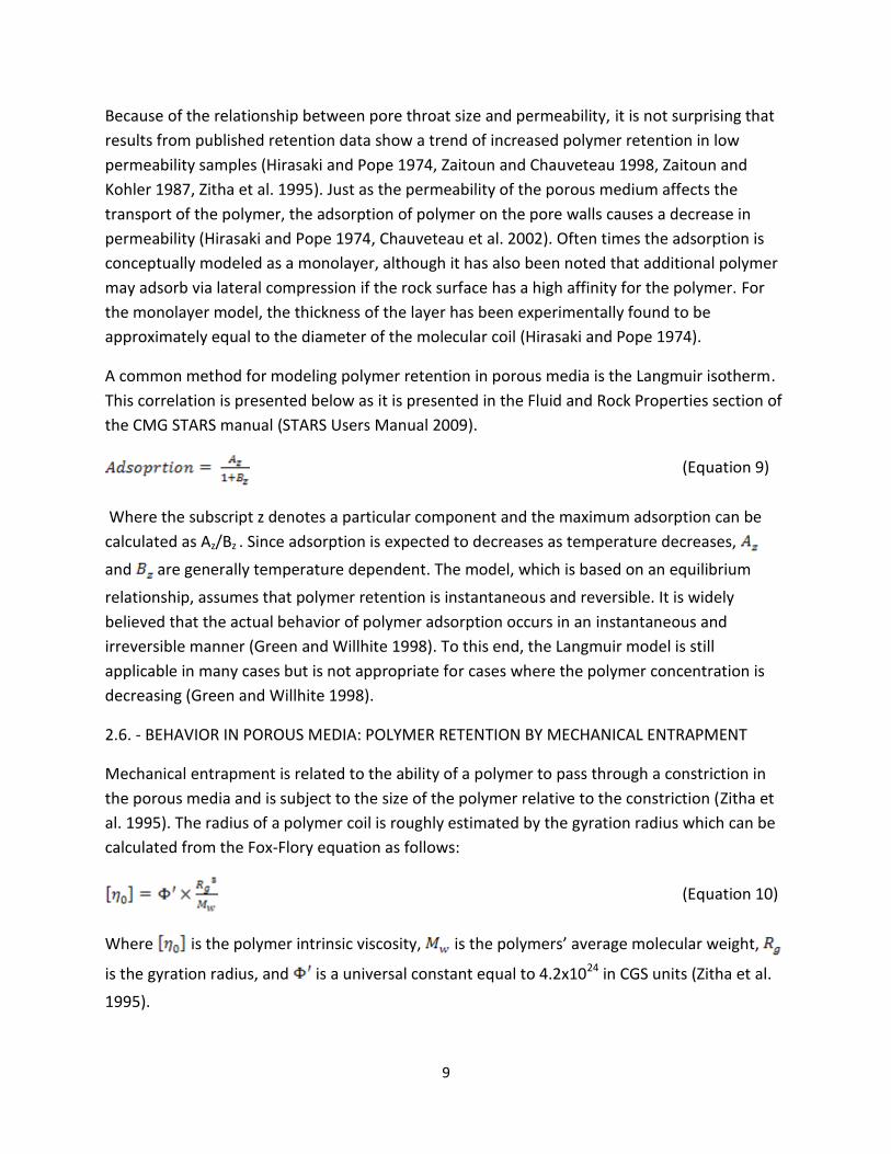
A common method for modeling polymer retention in porous media is the Langmuir isotherm.

This correlation is presented below as it is presented in the Fluid and Rock Properties section of

the CMG STARS manual (STARS Users Manual 2009).

(Equation 9)

Where the subscript z denotes a particular component and the maximum adsorption can be

calculated as Az/Bz . Since adsorption is expected to decreases as temperature decreases,

and are generally temperature dependent. The model, which is based on an equilibrium

relationship, assumes that polymer retention is instantaneous and reversible. It is widely

believed that the actual behavior of polymer adsorption occurs in an instantaneous and

irreversible manner (Green and Willhite 1998). To this end, the Langmuir model is still

applicable in many cases but is not appropriate for cases where the polymer concentration is

decreasing (Green and Willhite 1998).

2.6. - BEHAVIOR IN POROUS MEDIA: POLYMER RETENTION BY MECHANICAL ENTRAPMENT

Mechanical entrapment is related to the ability of a polymer to pass through a constriction in

the porous media and is subject to the size of the polymer relative to the constriction (Zitha et

al. 1995). The radius of a polymer coil is roughly estimated by the gyration radius which can be

calculated from the Fox-Flory equation as follows:

(Equation 10)

Where is the polymer intrinsic viscosity, is the polymers’ average molecular weight,

is the gyration radius, and is a universal constant equal to 4.2x1024 in CGS units (Zitha et al.

1995).

10

An alternative method for calculating the gyration radius, which was suggested for the research

which this thesis aims to model, is as follows (Stavland et al. 2010):

(Equation 11)

Where is the radius of gyration, A is the cross sectional area of the capillary tubes, is the

molecular weight associated with the polymer, and b takes a value between .5 and .6 for

random coil molecules (Stavland et al 2010). The Hagen-Poiseuille flow model, which

approximates the porous media as a bundle of capillary tubes, can be used to estimate the

average pore radius (Hirasaki and Pope 1974, Zitha et al. 1995). The pore radius is calculated in

this method as follows:

(Equation 12)

Where k is the permeability, and is the porosity for the porous medium.

Experimental studies have linked mechanical entrapment of flexible coiled polymers to a

dependence on the flow regime via the flow rate (Chauveteau et al. 2002). At low shear rates

associated with the Newtonian flow regime, the HPAM molecules remain in a coiled state and

tend to pass easily through pore constrictions. As the shear rates increase and shear thinning

begins, the polymers are slightly, but not permanently, deformed by the associated shear

forces. Increasing the shear rates further will lead to strong enough shear forces that the

polymers are elongated and shear thickening behavior is exhibited (Delshad et al. 2008,

Chauveteau et al. 2002, Green and Willhite 1998). Since the polymers do not have enough time

to return to their relaxed conformation between successive pore constrictions, the polymers

are propagated through the reservoir in an elongated state (Delshad et al. 2008, Heemskerk et

al. 1984, Hirasaki and Pope 1974). If these elongated polymers are adsorbed, especially near

entrances to constrictions where hydrodynamic forces are the largest, the result could be

bridged and blocked pore throats (Zaitoun and Kohler 1987, Zitha et al. 1995).

Although some earlier works suggest the polymer concentration has little effect on the

adsorption (Green and Willhite 1998), the concentration of the polymer has been

demonstrated to have an effect on pore plugging (Zaitoun and Chauveteau 1998, Zitha et al.

1995). As can be expected, injecting higher concentrations of polymer will lead to larger

amounts of pore plugging and pore blockage than the injection of lower concentrations of

polymer (Zaitoun and Chauveteau 1998, Zitha et al. 1995). At the same time, lower polymer

concentrations have larger stretched lengths than a higher polymer concentration for a give

shear rate (Zitha et al. 1995). Since the retention associated with pore throat blockage is a

11

function of how elongated the polymer molecules are, the larger stretched lengths of the lower

concentration polymer can still result in blocked pores (Zitha et al. 1995).

2.7 - BEHAVIOR IN POROUS MEDIA: THE INACCESSIBLE PORE VOLUME

The volume of the pore space that is not able to conduct polymer flow due to the large size of

the molecules relative to the pore passage ways is referred to as the inaccessible pore volume

(IPV). During the coreflood experiments conducted by Stavland et al. (2010), the apparent

viscosity values calculated for low injection rates resulted in lower values than the bulk

rheology would suggest. This behavior, which has also been reported by other researchers

(Zaitoun and Kohler 1987), has been attributed to the inaccessible pore volume or a depleted

layer model. Conceptually, since the polymer is not able to flow through the whole pore space,

it only travels through the accessible portion which results in an accelerated arrival at the

outlet. Models that reflect this concept have been developed by Sorbie (1991).

For the purpose of this work, the IPV can be calculated as follows (Stavland et al. 2010):

(Equation 13)

Where B is a constant with a physical meaning of (kw/kp) and can be derived from the pore

geometry. Assuming the porous media behaves as a bundle of capillary tubes, the B factor can

be calculated as:

(Equation 14)

Where d is defined as a thickness close to the wall (associated with the polymer monolayer),

and R is the radius of the capillary tube. Alternatively, the B factor can be determined by its

relationship to permeability reduction. An idealized way to calculate the permeability reduction

or RRF, which is based on the assumptions made for Hagen-Poiseuille flow, is as follows (Zitha

et al. 1995):

(Equation 15)

As with the equation used to calculate the B factor, d is the thickness of the layer of adsorbed

polymer, and R is the capillary radius. Thus by assuming Hagen-Poiseuille flow, an association

between RRF and the B factor can be made (Stavland et al 2010). This is a useful association, as

will be seen later, since the permeability reduction can be determined from experimental

pressure drop data.

12

More recent studies have demonstrated that high flow rates can result in additional adsorption

of polymer to the already existing monolayer on the pore wall. Experimental results from

polymer flow tests suggest that, above a critical rate the adsorbed layer thickness increases

with the volumetric rate of injection (Chauveteau et al. 2002, Zitha et al. 1995).

2.8 - BEHAVIOR IN POROUS MEDIA: THE APPARENT VISCOSITY

The four flow regimes that were detailed earlier provide a general idea of how polymer

solutions respond to different shear rates. Again, those regimes are Newtonian, shear thinning,

shear thickening, and degradation. Understanding how experimental rheological data relates to

polymer flow in porous media is of practical value which is why much time and effort is spent

on developing models for properties like apparent viscosity.

The following section focuses on methods used to determine apparent viscosity in porous

media. The first method utilizes core flood pressure drops to formulate parameters which can

be used to calculate experimentally determined apparent viscosity values. Although this

method provides correct results, it is fairly uncommon for a company to have this level of data

when modeling a polymer flood. A new analytical model has recently been developed which

accurately determines the apparent viscosity by means rheological data along with minimal

core flood data (Stavland et al. 2010). The experimental data that was used to develop this new

model is also used as input for the simulation described later in this paper.

2.9 - APPARENT VISCOSITY FROM CORE FLOODS

In core flood experiments, it is not possible to directly measure the apparent viscosity in a

flooding experiment. Instead the apparent viscosity is determined by equations that depend on

the mobility reduction (RF) and the permeability reduction (RRF). The permeability reduction

has been found to depend on the size of the polymers (Zitha et al. 1995). The relationship

between the two is such that, as the molecular weight of the polymers increases, the

permeability reduction also increases (Hirasaki and Pope 1974). The mobility reduction and the

permeability reduction utilize pressure drop ratios to create a non-dimensional representation

of the altered permeability and mobility due to polymer flooding (Chauveteau et al. 2002,

Green and Willhite 1998, Zitha et al. 1995). The equations for both parameters are as follows:

(Equation 16)

(Equation 17)

Where is the pressure difference due to the flow of brine before polymer is injected

and is the pressure difference due to the flow of brine after polymer is injected.

13

An assumption is made regarding the variable , where the brine permeability after

polymer flow is the same as the polymer permeability (Chauveteau et al. 2002, Green and

Willhite 1998, Hirasaki and Pope 1974, Zitha et al. 1995). For consistency, the pressure drops

used in the pressure ratios should be determined at the same flow rate. The experimentally

derived apparent viscosity is calculated by taking the ratio of the mobility reduction to the

permeability reduction as follows (Stavland et al. 2010):

(Equation 18)

The brine viscosity in this equation is roughly close to one.

2.10 - APPARENT VISCOSITY: GRAPHICAL RESULTS

The following plot of mobility reduction displays the aforementioned flow regimes with relation

to shear rate.

Figure 2.3: Flow regime behavior and trends in mobility reduction data as a function of shear rate

14

This plot exemplifies the small scale of the shear thinning behavior compared to the shear

thickening behavior. The large magnitude of the shear thickening behavior relative to the shear

thinning behavior has been previously reported by Seright et al. (2010). In the following plot the

shear thickening and degradation regimes are very prominent compared to the shear thinning

regime.

By calculating the apparent viscosity from the previous equation for the core flood data, the

apparent viscosity can also be plotted as follows:

Figure 2.4: Flow regime behavior and trends in apparent viscosity data as a function of shear rate

The apparent viscosity in Figure 2.4 reaches a maximum of roughly 7.5 cp. This value is quite

small compared to the apparent viscosity values which were achieved by the polymers which

will be discussed later in this paper. Even so, the expected trends are present with regards to

shear thickening and degradation.

2.11 – THE RELATIONSHIP BETWEEN SHEAR RATE AND INTERSTITIAL VELOCITY

For the purpose of conducting rheological experiments, it is common to record the polymers

behavior with relation to the shear rate. When considering polymer behavior in porous media,

it is more natural to think in terms of Darcy velocities or volumetric rates. There are many

15

equations that have been proposed to relate shear rate to the interstitial velocity, and it is

common for tuning parameters and adjusting factors to be utilized so the data is properly

aligned (Sorbie 1991). For the purpose of this paper, the following relationship was used to

relate shear rate to interstitial velocity (Stavland et al. 2010):

(Equation 19)

Where is the interstitial velocity, is the porosity, and is the permeability. An -value of 2.5

was used since this value is what has been deemed appropriate for porous media with angular

particles (Zitha et al. 1995).

CHAPTER 3 - EXPERIMENTAL COREFLOOD DATA

3.1 - INTRODUCTION TO THE EXPERIMENTAL DATA

The simulation work created for this thesis was based on experimental data provided by two

separate sources. Both sources used a polymer which was 30% hydrolyzed, mixed into synthetic

seawater, and had a molecular weight of 20 million Dalton. This polymer was also known by the

name 3630SSW.

One of the data sets resulted from the experiments conducted by Stavland et al. (2010) using

Berea sandstone cores. These experiments studied the polymer behavior in single phase flow,

so the initial core saturations before polymer flooding were 100% synthetic seawater.

The other experiment, which was conducted using a Bentheim sandstone core, was used to

study the polymer behavior in two phase flow where the initial saturations consisted of oil at a

residual saturation and synthetic seawater (Moradi 2011). The rest of this chapter is dedicated

to explaining the procedures and results associated with these two experiments in more detail.

3.2 – THE SINGLE PHASE EXPERIMENTS

3.2.1 – PREMISE FOR THE SINGLE PHASE EXPERIMENTS

Recently conducted research (see for example, Stavland et al. 2010) has aimed to develop an

equation to model the shear degradation behavior which has been observed at very high shear

rates, from a combination of bulk and core rheological data. Polymer experiments were

preformed where parameters such as molecular weight, permeability, degree of hydrolysis, and

brine salinity were systematically altered and the apparent viscosity was determined

16

experimentally. The resulting apparent viscosity values were well-matched with a theoretical

model.

3.2.2 – PROCEDURE FOR THE SINGLE PHASE EXPERIMENTS

Bulk viscosity measurements were preformed for multiple polymer solutions which varied with

concentration, molecular weight, and degree of hydrolysis. From the bulk experiments,

relaxation times and shear thinning exponents were determined for the polymer mixtures

(Stavland et al. 2010).

The core flood experiments were conducted using two serially mounted cores each of which

had a 1.5 inch diameter and were 7 centimeters in length. Before the polymer injection began,

the cores were initially 100% saturated with synthetic seawater (SSW). Additionally, the

reference makeup water for the polymer was synthetic seawater. Once the polymer injection

process began, the two cores were exposed to sequential increases and decreases in injection

rate. During the injection process, atmospheric pressure was maintained at the outlet of the

second core. The pressure drop in each core section was determined as a function of time by

using a pressure tap located between the two cores. When the pressure drop for a given rate

was assuredly stabilized, pressure data was recorded, and a new flow rate was initiated.

At the end of the series of injection rates, water was injected and the pressure drop was

recorded. This pressure drop was then used to determine the permeability reduction. Since

each set of the two serially mounted cores was exposed to multiple flow rates, only one value

of permeability reduction (RRF) was determined for the polymer solution. Given that the first

flow rate is maintained until steady-state flow is achieved, it is generally assumed that all of the

adsorption will occur during this flow rate.

In some situations however, an increase in flow rate could lead to an increase in permeability

reduction (Chauveteau et al. 2002). As previously discussed, in the Newtonian and the shear

thinning flow regimes, the polymers are not elongated and are in a relaxed conformation. If the

flow rate increases and the polymers elongate, hydrodynamic retention could result

(Chauveteau et al. 2002, Zaitoun and Chauveteau 1998, Zitha et al. 1995). This might cause an

increase in permeability reduction if the retention is permanent. If additional polymer adheres

to the polymer that has already adsorbed, the permeability reduction may further increase

(Chauveteau et al. 2002). Therefore, if fresh cores were used for each new flow rate in the

experimental procedure described above, one could argue that a different RRF might be

achieved for each flow rate. For the purposes of this thesis, the single RRF value associated with

the polymer will be used as a guide to allow for the proper pressure drop to be achieved in the

history match.

17

3.2.3 – RESULTS THE SINGLE PHASE EXPERIMENTS

The experimental data which was reported by Stavland et al. (2010) for the 3630SSW HPAM

solution with a molecular weight of 20 million Dalton and 30% hydrolysis was of special interest

for this thesis. The following section provides more details about the results from the bulk and

core flood experiments for this particular polymer solution.

A summary of the core properties are as follows in Table 3.1

Location Diameter Length Porosity Permeability

Front 1.5 inches 7 cm 0.22 824 mD

Back 1.5 inches 7 cm 0.22 800 mD

Core Properties

Table 3.1: Core properties for the single phase experiment

Both cores were comprised of Berea sandstone, but the permeability properties in the front

core differed very slightly from the properties in the back core. During polymer injection, the

front core experienced very high pressures due to polymer alignment and adjustment in the

pore space. Since the polymer behavior was more stable as it flowed through the second core,

the experimental results from the second core were the focus of the history matching

simulations.

From the bulk rheology experiments, the relaxation time and shear thinning exponents were

determined as a function of normalized polymer concentration. The intrinsic velocity, relaxation

time, and shear thinning exponent for the 3630SSW polymer are displayed in Table 3.2

Table 3.2: Bulk rheology data for the 1500 ppm polymer

18

By using these experimentally derived parameters in the Carreau model it was possible to

create a graph of bulk viscosity as a function of shear rate which can be seen in Figure 3.1. As

expected, the polymer behavior displays both lower Newtonian and shear thinning behavior.

For this particular plot, the shear rates do not extend to high enough values to display the

upper Newtonian behavior which would asymptotically approach the viscosity of the synthetic

seawater.

Figure 3.1: Experimental results for the bulk viscosity of the polymer as a function of shear rate

19

Pressure measurements in the front and back core were obtained every half minute during the

flooding experiment. In Figure 3.2, the pressure drop in the back core has been plotted as a

function of time along with the associated injection rate. As previously mentioned, the data

from the back core was the only data considered when simulating the flooding experiment. The

pressure spikes that can be seen at the beginning of each new flow rate were a result of the

polymer realignment that occurred when the macromolecules elongated with increasing

injection rates. For the injection rates that occur in the degradation regime, an initial pressure

spike can be attributed to an entrance pressure drop which occurs when the polymer shreds as

it enters the formation (Seright 1983).

0.001

0.01

0.1

1

10

100

0 100 200 300 400 500 600 700 800

Pre

ssu

re D

iffe

ren

ce (b

ar)

Time (min)

Experimental Pressure Results and Injection Rates for the Back Core

Injection Rate

Pressure Drop

Figure 3.2: Polymer injection rates and resulting pressure differentials across the back core

20

The stabilized pressure drop associated with steady state flow was also recorded for each flow

rate. This data is presented for the back core in Table 3.3 along with the injection rate.

Flow RatePressure Drop:

Back Core

ml/min bar

2 2.49

4 5.08

5 6.02

6 6.74

7.5 7.5

10 8.46

12.5 9.2

15 9.63

20 9.64

3 3.89

2 2.5

1.5 1.45

1 0.512

0.5 0.139

0.2 0.0519

0.1 0.0293

0.05 0.0179

0.02 0.00825

Table 3.3: Stabilized pressure difference for various flow rates in the second core

21

The polymer-related pressure drops in the second core for a given flow rate were used in

conjunction with water-related pressure drops to determine the mobility reduction. The plot in

Figure 3.3 displays the mobility reduction data with respect to volumetric flow rate.

0

20

40

60

80

100

120

140

0.01 0.1 1 10 100

RF,

Mo

bili

ty R

edu

ctio

n

Volumetric Flow Rate (ml/min)

Mobility Reduction vs. Flow Rate

Figure 3.3: Flow regime trends in experimentally determined mobility reduction data as a function of flow rate

The pressure drop values associated with each flow rate for water were calculated using

Darcy’s Law and the core properties of the back core. These water flood pressure drop values

were also modeled in the simulator for the aforementioned experimental core set-up. The

values determined from the Darcy’s Law calculations matched very well with the values from

the water flood simulation. The procedure taken to model the simulated water flood will be

discussed in more detail in Section 4.3.2.

In the experiments preformed by Stavland et al. (2010), after multiple rates of polymer

injection, a second water flood was preformed until steady-state flow was achieved. From the

stabilized pressure drop associated with this water injection, the permeability reduction (RRF)

was determined to be 3.6.

22

Given that the mobility reduction, permeability reduction, and water viscosity (taken to be 1.08

cp) are known, the experimentally derived apparent viscosity can be determined as described

by Equation 18. The apparent viscosity calculated by this method is displayed in Figure 3.4. The

mobility reduction values were initially determined with respect to the volumetric flow rate,

but through the relationship presented earlier, these flow rates have been converted to shear

rates.

0

5

10

15

20

25

30

35

40

1 10 100 1000 10000

Ap

par

en

t Vis

cosi

ty (c

p)

Shear Rate (1/sec)

Apparent Viscosity vs. Shear Rate

Figure 3.4: Flow regime trends in experimentally determined apparent viscosity data as a function of flow rate

The importance of displaying the apparent viscosity with respect to shear rate is that it

highlights the difference in polymer behavior between the rheological results and the core

flood results. For the range of shear rates presented above, shear thickening and degradation

behavior is very prominent in the core flood. For a very similar range of shear rates, the

rheological bulk data is dominated by a shear thinning regime.

Table 4.1 (located in the water flood simulation section), presents the mobility reduction,

apparent viscosity, and pressure drop values in a consolidated form along with the injection

rate.

23

3.2.4 – THE APPARENT VISCOSITY MODEL

In the earlier sections of this work, which covered the individual flow regimes, viscosity

equations were developed based on the behavior in each regime. Recent research, which

focused on relating shear degradation to rheological properties, has resulted in an equation

which accurately models the behavior of all four flow regimes (Stavland et al. 2010).

As discussed in the section on shear thickening, earlier models have been developed which

accurately handle the shear thickening regime. Furthermore, Delshad et al. (2008) produced a

well-matched simulation of the shear thickening regime using the UTCHEM simulator.

The new developments by Stavland et al. (2010) have created a successful model of the

degradation regime which occurs at very high shear rates. This model has demonstrated a

capability to match apparent viscosities derived from experimental core floods. The model is as

follows:

(Equation 20)

Where the time constant, , is determined from bulk viscosity measurements. Additionally,

two experimentally derived relationships were used to determine and where / = 17,

and / = 238. (Stavland et al. 2010)

The apparent viscosity at zero shear rate, , which is associated with flow through porous

media and is calculated as:

(Equation 21)

Here, is the polymer solution viscosity at zero shear rate, is the water viscosity, and B is a

factor related to the inaccessible pore volume (IPV). The B-factor can be determined through a

relation with the RRF as discussed in the section on retention. The relationship between the B-

factor and the RRF is based on the idealized assumptions made for Hagen-Poiseuille flow. Since

the B-factor cannot be determined experimentally, it may also function as a tuning parameter.

24

Figure 3.5 displays the resultant apparent viscosity for the 3630SSW HPAM polymer as

determined by Equation 20.

0

5

10

15

20

25

30

35

40

45

10 100 1000 10000 100000

Ap

par

en

t Vis

cosi

ty (c

p)

Shear Rate (1/sec)

Apparent Viscosity:Experimental Based and Model Based

1500 ppm, 2030

Experimental

Figure 3.5: A comparison of experimental-based and model-based apparent viscosity values

The graphical results displayed above were part of the data used to investigate whether or not

current simulation technology had the proper functionalities to simulate this recently modeled

behavior.

3.3 – THE TWO PHASE EXPERIMENTS

3.3.1 – PREMISE FOR THE TWO PHASE EXPERIMENTS

Moradi in 2011 preformed multiple coreflood experiments of oil displacement by polymer

solutions and under various core-wetting conditions. As compared to the previous experimental

work which occurred as single phase flow, this new experimental work focused on the behavior

that occurred when oil was also present in the core. Aside from creating new insight to the

specifics of two phase polymer flooding behavior, his work also provided input data that could

be used for modeling in a simulator.

25

3.3.2 – EXPERIMENTAL PROCEDURE FOR THE TWO PHASE COREFLOOD

The polymer which was studied in the two phase core flood was described as being 30%

hydrolyzed with a molecular weight of 20 million Dalton. Synthetic seawater was used as the

makeup water for the polymer solution.

A bulk rheology study was conducted for this polymer solution at multiple concentrations

varying between 100 and 2000 ppm. For each polymer concentration, the bulk rheological

behavior was observed as the shear rate was varied from low to high and high to low values of

shear rate. The data from the experiments that went from high to low shear rates were the

clearest, and were therefore taken to represent the bulk behavior of the polymer solution.

For this particular experiment, a single water-wet Bentheim core was used for the flooding

process. After the core was loaded into the core holder and put on a vacuum, synthetic

seawater was injected until the core was saturated. Once it was verified that the core was 100%

saturated with synthetic seawater, the absolute permeability of the core was determined using

data collected during multiple injection rates of the synthetic seawater. The core was then

flooded with oil until residual water saturation was established which was then followed by

another water flood using synthetic seawater to establish a residual oil saturation.

At this point the core saturations consisted of residual oil and water, which meant polymer

flooding could commence. The polymer was injected at an intentionally low rate in order to

maintain the residual oil saturation establish by the previous water flood. Additionally, since

this was the first polymer injection the core had experienced, it is assumed that most of the

irreversible adsorption and retention took place during this injection process.

After injecting about 4.2 pore volumes of polymer in the core, another injection of synthetic

seawater occurred. The purpose of this flood was to remove the non-adsorbed polymer before

performing a second polymer flood to study the retention of the polymer in the core. Because

both polymer injection processes were conducted at the same rate, the difference in the

injected pore volumes required to reach steady-state flow are attributed to the polymer

retention.

Finally, a multi-rate polymer flood was conducted. For the first three increasing rates, no visible

oil was produced and the residual oil saturation remained the same as it was initially. For the

fourth rate and on, visible volumes of oil were produced. These volumes were recorded and

used to determine the new residual oil saturation once both steady-state flow occurred and no

additional oil production was seen. The experimental results that were provided as the basis for

the two phase simulation are detailed in the following section.

26

3.3.3 – RESULTS FROM THE TWO PHASE EXPERIMENTS

The bulk rheology measurements from the experiments conducted by Moradi in 2011 are

presented in Figure 3.6. The different cases, each of which has been fit with a Carreau model,

represent the aforementioned polymer at different concentrations.

1

10

0.1 1 10 100 1000

Vis

cosi

ty (c

p)

Shear Rate (1/s)

High to Low shear rate3630 in SSW

C.M 2000 ppm

C.M 1500 ppm

C.M 1000 ppm

C.M 750 ppm

C.M 500ppm

C.M 250 ppm

C.M 100 ppm

2000 ppm

1500 ppm

1000 ppm

750 ppm

500 ppm

250 ppm

100 ppm

Figure 3.6: Experimental bulk rheology data and corresponding Carreau model for various polymer concentrations

The concentrations below 1000 ppm display a very small increase in viscosity towards the

highest shear rates that were encountered. Although it is probably not appropriate to refer to

this trend as “shear thickening,” given the small magnitude of the behavior, it is an interesting

occurrence. Additionally it should be noted that at lower concentrations, the polymers display

erratic behavior and do not adhere to the Carreau model as well as the higher concentration

polymer solutions. For the purpose of this work, the behavior of the polymers at lower

concentration is of special interest since the polymer that was modeled in the simulator had a

concentration of 400 ppm.

27

Table 3.4 contains information about the core dimensions, porosity, and absolute permeability

as determined from the multi-rate water flood. This water flood occurred before polymer was

injected, so the calculated absolute permeability does not reflect any effects from polymer

retention.

Diameter Length Porosity Permeability

3.794 cm 24.3 cm 21.34% 2278.76 mD

Core Properties

Table 3.4: Core properties for the two phase experiment

The end-point relative permeability values were determined by conducting a water flood at

residual oil saturation, and an oil flood at residual water saturation. Again, both of these

injection cycles occurred before any polymer was introduced in the core, so the measurements

were unaffected by polymer retention. Table 3.5 displays the end-point saturation and relative

permeability information that was gathered from this experiment.

22.82%

1607.27 mD

0.705327

39.92%

216.41 mD

0.09497

Oil Relative Permeability at Swi

Water Flooding at Residual Oil Saturation

Residual Oil Saturation (Sor)

Water Permeability at Sor

Water Relative Permeability at Sor

Relative Permeability and Saturation Values

Before Polymer Flooding

Oil Flooding at Interstitial Water Saturation

Interstitial Water Saturation (Swi)

Oil Permeability at Swi

Table 3.5: Relative permeability and saturation values for the Bentheim core before polymer flooding

When the polymer flooding began, it was intentionally conducted at a very low rate in order to

avoid oil production. By doing this, the effects from the polymer could be analyzed without any

convoluting effects from two phase flow being mixed in. Plots of the pressure difference across

the core from the primary and secondary polymer floods are presented in Figures 3.7 and 3.8,

respectively.

28

Figure 3.7: Differential pressure drop across the core during the initial polymer injection

Figure 3.8: Differential pressure drop across the core during the second polymer injection

29

During the primary polymer flood, about one pore volume was injected at a rate of .2 mL/min

before steady-state was achieved. The secondary polymer flood only required about .5 pore

volumes before the pressure difference achieved steady-state. Between each of the polymer

floods, a water flood was conducted to clean out the excess polymer that had not adsorbed to

the rock surface. Given that both polymer floods were conducted at an injection rate of .2

mL/min, the difference between the volumes that were injected to reach steady-state was

attributable to the retention that occurred during the primary polymer flood.

After the polymer flood occurred, the relative permeability was reassessed to determine the

permeability properties associated with the polymer. Additionally, the permeability reduction

was determined to be 1.3958 by comparing the permeability of the polymer and the water

flood at residual oil saturation. Table 3.6 presents the polymer flood associated end-point

results.

39.92%

155.041 mD

0.068038

Relative Permeability and Saturation Values

After Polymer Flooding

Polymer Flood at Residual Oil Saturation

Residual Oil Saturation (Sor)

Polymer Permeability at Sor

Polymer Relative Permeability at Sor

Table 3.6: Relative permeability and saturation values for the Bentheim core after polymer flooding

A series of multi-rate polymer injections were conducted right after the second .2 mL/min

polymer flood. The order of the injection rates for the multi-rate polymer flood was as follows:

.4, .8, 1.6, 3.2, 6.4, 9.6, 12, 14, and 18 mL/min. No delay occurred between the second polymer

flood at an injection rate of .2 mL/min and the .4 mL/min injection rate. The experimental data

that was recorded during these injection rates is presented in two separate figures. The first

plot (Figure 3.9) shows the data collected for the flow rates varying from .2 mL/min to 3.2

mL/min and the second plot (Figure 3.10) shows the data collected for the flow rates varying

from 6.4 mL/min to 18 mL/min.

30

Figure 3.9: Differential pressure drop across the core for the first five injection rates

Figure 3.10: Differential pressure drop across the core for the last five injection rates

All of the injection rates that occurred before the injection rate of 3.2 mL/min resulted in single

phase flow and were therefore conducted at the same residual oil saturation as the one posted

in the previous table. The larger injection rates, starting with the injection rate of 3.2 mL/min ,

produced oil along with the injected polymer which meant a new residual oil saturation was

established during each of these flow rates.

31

For the purpose of this thesis, the largest injection rate that was considered for simulation work

was 3.2 mL/min. The oil produced during this rate amounted to 1.1 mL which resulted in a

decrease of the residual oil saturation from its previous value of 39.92 % to a value of 38.04%.

CHAPTER 4 - SIMULATION WORK AND RESULTS

4.1- SELECTING A SIMULATOR

Before any simulation work could take place, a simulator had to be selected. There were two

main qualities which were sought after when deciding which simulator was most applicable.

First, it was necessary that the simulator had the capacity and the functionalities necessary for

modeling the polymer behavior of interest. For example, since the degradation behavior was of

particularly important, it was necessary that the selected simulator could model this behavior.

It was also desirable for the simulator to be commonly used within the industry. Since the

ultimate purpose of conducting the polymer experiments was to gain a better understanding of

the polymer behavior for what would eventually be field purposes, it is also important that a

commonly available simulator could model the experimental findings.

The three simulators which were investigated for potential use were Eclipse which has been

created by Schlumberger, STARS which has been created by CMG, and UTCHEM which has been

created for research application at the University of Texas at Austin. The ability of UTCHEM to

model a polymer solutions shear thickening behavior had already been demonstrated by

Delshad et al. (2008). Other attractive features of this simulator included the availability of the

source code, its specialized ability to model lab scale experiments, and the fact that it was

specially designed to model very specific and complex chemical and polymer behavior. The

obvious downfall of this simulator is the fact that it is not commonly used outside of the

academic realm.

The Eclipse simulator is by far one of the most well known reservoir simulation tools in the

petroleum industry. Because it is so commonly used in the industry for field applications, it

could have been an ideal simulator for modeling the experiments. Unfortunately, this very

popular simulator did not contain the technical functionalities required to model the recent

experimental findings that were the focus of this work. At the time of the investigation, the

polymer viscosity related capabilities of the Eclipse simulator were restricted to shear thinning

behavior. Although the simulator also had the capacity to model salinity effects, adsorption

behavior, and polymer concentration mixing behavior, without the ability to model the shear

thickening and degradation regimes, a successful simulation could not be produced.

32

The final simulation tool which was considered and subsequently selected to model the

experimental data was the STARS simulator by CMG. This simulator, which is implemented by

multiple companies in the petroleum industry, is known for its ability to model both laboratory

and field scale models while also having the capability to handle complicated chemical

behavior. One of the main attractive features of this simulator was option to input the polymer

apparent viscosity in a tabular format. Although it was not certain from the outset, the hope

was that the tabular input would be able to handle all four flow regimes if necessary. Further

details regarding the polymer-related keywords which were applicable for this work are

discussed in the following section.

4.2- KEYWORDS FOR THE CMG STARS SIMULATOR

An important preliminary step towards creating a successful simulation model required gaining

a better understanding of the simulator and how it functioned. Given that the STARS simulator

operates through the usage of keywords, it was important to understand which keywords were

applicable to the polymer model, how the keywords worked, and what inputs were required for

the keywords to function properly. The keywords discussed here are presented in the order in

which they appear in the simulator. It is important to note that the simulation model was

developed via a data file rather than through the interface provided by STARS.

The first polymer-related keyword that is encountered in the simulation code is “VSMIXFUNC,”

which handles the non-linear viscosity behavior that results from the changes in the polymer

concentration. The manner in which the water phase viscosity increases as the polymer

concentration increases can be modeled from bulk rheology data if experiments are conducted

for multiple polymer concentrations. The concentration mixing behavior affects how quickly the

viscosity builds in the polymer front, which in turn affects how quickly the pressure builds in the

model. By default, the simulator assumes a linear mixing behavior when the user does not

supply input values.

When a linear mixing behavior is not realistic, the keyword allows for eleven inputs, each of

which will be associated with equally spaced polymer concentrations varying from zero to a

given concentration of interest. The polymer concentration range is specified with the

associated keyword, “VSMIXENDP.” The eleven inputs used with the “VSMIXFUNC,” keyword

are used to correct the curvature of the actual viscosity-concentration behavior to that of a

linear trend. The specific linear trend to which the data is fit is described by a line connecting

the viscosity associated with zero polymer concentration, and the viscosity associated with the

maximum polymer concentration of interest.

Once the mixing behavior is accounted for, the “SHEARTAB,” keyword is used to model the

apparent viscosity that occurs for a given flow rate and reflects the behavior associated with

33

the maximum polymer concentration as set by “VSMIXENDP.” The keyword, which allows for 40

input values, allows the user to define the polymer viscosity as a function of the Darcy velocity.

The data is input as two columns, the first of which is for the Darcy velocity, and the second of

which is the associated apparent viscosity. In this work, there were two methods used to create

the apparent viscosity data. As previously discussed, the apparent viscosity can be determined

from experimental data as a function of the permeability and mobility reduction values. If this

data is not available, and only a single phase is flowing, the Darcy equation can be used to

create an approximation for these inputs.

The remaining pertinent keywords which have yet to be discussed are all related to the

adsorption behavior and are grouped together in the simulator. The first of these adsorption

keywords is “ADSTABLE,” which essentially provides a tabular method for inputting data related

to the Langmuir isotherm. The input table consists of two columns of data. The first column

contains the polymer concentration values and the second column contains the adsorption

values associated with each concentration. Since the Langmuir isotherm is a commonly used

method for attributing adsorption behavior to specific polymer concentrations, the STARS

simulator also offers the option of specifying the Langmuir model according to the isotherm

coefficients. Additionally, the simulator allows for the “ADSTABLE,” and the “ADSLANG,”

keywords to reflect temperature dependence, but this feature was not used for this thesis.

Since the adsorption parameters can vary for different rock types, and it is possible to have

multiple rock types in a reservoir, the simulator is capable of defining different rock types

within a single model. Although it was not necessary to define multiple rock types for this

thesis, the following adsorption keywords could have been used in a manner that defined

multiple rock types. For the purpose of this thesis, they were used accordingly to represent a

single rock type.

The first of these parameters is the maximum adsorption capacity which is accounted for by

the keyword “ADMAXT.” The irreversible adsorption behavior, which is related to the maximum

adsorption capacity, is modeled with the keyword “ADRT.” Both the maximum adsorption and

the irreversible adsorption used the same units.

The inaccessible pore volume was handled with the “PORFT,” keyword which is more accurately

described as the percentage of accessible pore volume. The “PORFT,” input value can be

calculated as (1-IPV). The final adsorption keyword was the permeability reduction or “RRFT.” In

the STARS simulator, when the “RRFT,” is set equal to one, there is no permeability reduction

effect. The “PORFT,” and “RRFT,” keywords operate as a function of how much polymer has

been adsorbed compared to the stated maximum adsorption. Once the maximum adsorption is

achieved, the full effect of the “PORFT,” and “RRFT,” values are seen in the simulator. For

34

adsorption values smaller than the maximum adsorption, the “PORFT,” and “RRFT,” are only

seen as a fraction of the input values.

4.3 – SINGLE PHASE SIMULATION WORK

4.3.1 – INTRODUCTION TO THE SINGLE PHASE SIMULATION WORK

Using the data that was collected as a result of the single phase flow experiment, which was

described in the previous chapter, the following simulation work was created. While obtaining a

well matched simulation was considered an important task, it was imperative that the input for

the simulated model did not deviate too much from the experimentally determined

parameters. For this reason, only parameters such as adsorption, which was not well defined,

and the permeability reduction value, which might vary slightly with flow rate, were considered

to be tuning parameters.

4.3.2 – MODELING A WATERFLOOD

A water flood was simulated before attempting to simulate and history match the polymer

flood data. This exercise was useful for gaining a better understanding of the simulator,

ensuring that the initialization parameters were set properly, and obtaining the pressure

difference in the core due to water injection at multiple rates. The water injection rates studied

with the simulator were the same rates the cores experienced during the experimental polymer

flood.

The water flood simulation was based on an example file provided by CMG STARS. The original

example file (see ‘stflu036,’ in the 2009 STARS example database) demonstrated how the

polymer-related key words were used to model an example polymer flood. By inhibiting the

irrelevant key words, setting the core parameters and initial conditions to be representative of

the experimental parameters, and adjusting the injection fluid to pure water, a successful water

flood was simulated.

The two serially mounted cores were modeled with 30 blocks each, or 60 blocks in total.

Injection and production wells were located in blocks one and 60, respectively. The pressure

tap which recorded the pressure between the first and second core in the lab experiment was

modeled by setting the simulator to record the block pressures in blocks 30 and 31. The

average pressure from these two blocks was taken to be the pressure recorded by the pressure

tap which is also the entrance pressure to the second core. The pressure drop in the second

core was determined from the difference between the average pressures in blocks 30 and 31,

and the pressure in the block 60, where the producing well was located.

35

The results from the water flooding simulations are located in Figure 4.1. The graph displays the

pressure difference between the inlet and outlet of the second core as well as the water

injection rate. As can be seen, the difference in the pressure increases or decreases

immediately for each increasing or decreasing flow rate.

Figure 4.1: Injection rates and pressure results for the simulated multi-rate water flood

36

The following table summarizes the results for the water flood pressure drop, mobility

reduction, and apparent viscosity values for different flow rates.

Flow RatePressure Drop:

Back Core

Simulation

Waterflood

Darcy-Based

WaterfloodRF

Calculated

Apparent

Viscosity

ml/min bar bar bar Unitless cp

2 2.49 2.251E-04 2.250E-04 36.66 10.69125607

4 5.08 5.626E-04 5.626E-04 31.82 9.279695656

5 6.02 1.125E-03 1.125E-03 26.04 7.594834713

6 6.74 2.250E-03 2.250E-03 23.06 6.726839757

7.5 7.5 5.626E-03 5.626E-03 24.71 7.206402483

10 8.46 1.125E-02 1.125E-02 45.50 13.27201231

12.5 9.2 1.688E-02 1.688E-02 85.91 25.05779161

15 9.63 2.250E-02 2.250E-02 110.65 32.27302088

20 9.64 2.250E-02 2.250E-02 111.09 32.4026314

3 3.89 3.376E-02 3.376E-02 115.24 33.61229997

2 2.5 4.501E-02 4.501E-02 112.87 32.92107351

1.5 1.45 5.626E-02 5.626E-02 107.01 31.21026416

1 0.512 6.751E-02 6.751E-02 99.84 29.11929329

0.5 0.139 8.439E-02 8.439E-02 88.88 25.92227447

0.2 0.0519 1.125E-01 1.125E-01 75.19 21.93035652

0.1 0.0293 1.406E-01 1.406E-01 65.41 19.07899077

0.05 0.0179 1.688E-01 1.688E-01 57.06 16.64235295

0.02 0.00825 2.250E-01 2.250E-01 42.84 12.49485843

Table 4.1: A summary of the water flooding results, mobility reduction, and apparent viscosity calculation

4.3.3 – SENSITIVITY STUDY: ADSORPTION PARAMETERS

After the water flood was correctly simulated, the polymer flood became the focus of the

simulation work. Although very good data was available to model the apparent viscosity, there

was not any experimental adsorption data available. Additionally, viscosity data was only

available for one concentration, so the viscosity behavior of the polymer at lower

concentrations was relatively unknown. Because a mixing front is developed as the polymer

front travels through the core, understanding the viscosity effects for the lower concentrations

allows for the viscosity of the front to be simulated accurately. As previously mentioned, the B-

factor can behave as a tuning parameter and therefore the IPV (or PORFT with respect to the

STARS nomenclature) was considered a tuning parameter for the simulation.

37

The following list summarizes the parameters that were not known, and were considering

tuning parameters for the simulation.

The effect of polymer concentrations lower than 1500 ppm on the viscosity (i.e.: the

viscosity mixing rule)

Adsorption parameters including: the maximum adsorption, the adsorption associated

with different polymer concentrations (Langmuir isotherm), the amount of reversible

adsorption, and the resultant inaccessible pore volume (IPV).

Sensitivity studies were conducted for a range of realistic values in order to gain a better

understanding of how greatly these unknown parameters affected the simulation results. Since

the first flow rate used in the experimental procedure was 2 ml/min, the sensitivity study was

also conducted at this flow rate. This first flow rate was decidedly the most critical flow rate for

the purpose of achieving a proper history match since all of the effects from the polymer

adsorption and the mixing of polymer concentrations occur during this flow rate.

The initial sensitivity study was designed in order to gain a better understanding of the polymer

adsorption. It is understood that there is a maximum level of adsorption after which no more

polymer can be adsorbed. For the purposes of this work, it was assumed that most if not all of

the adsorption had occurred once the pressure drop achieved steady state. The maximum

adsorption, adsorption associated with the injected polymer concentration, and the irreversible

adsorption all used input units of moles per pore volume. The sensitivity study was conducted

assuming that a reasonable range of adsorption would be 5 to 30% of the injected polymer

moles. These adsorption percentages correspond to adsorption values (in units of moles per

pore volume) of 1.18x10-11 and 7.06x10-11, respectively. This range was studied in increments of

5%.

The first sensitivity that was to be executed would have investigated the effect of varying the

percentage of adsorption, while keeping the maximum adsorption, the adsorption associated

with polymer concentration, and the irreversible adsorption equal to each other. Unfortunately

the Langmuir isotherm-based adsorption table in STARS requires that the difference between

each entry not be smaller than 1x10-10 moles of polymer per pore volume. With respect to the

volume of solution injected, an adsorption of 1x10-10 moles per pore volume would mean that

around 42.5% of the injected polymer was adsorbed. Since the polymer adsorption associated

with the injected polymer concentration could not go low enough to realistically model the

adsorption behavior, it was set constant at 1x10-10 moles per pore volume while the maximum

adsorption and irreversible adsorption were varied.

38

Table 4.2 displays the inputs for the first sensitivity study, and Figure 4.2 displays the simulation

results from these input values. Each of the cases in the table corresponds, as labeled, to a

graphical simulation result. The experimental pressure difference for 2 ml/min flow rate is also

plotted with the simulation results as a dark charcoal colored line.

Table 4.2: Input data for the maximum and irreversible adsorption study - all adsorption parameters are in units of moles per pore volume

Figure 4.2: Simulation results for the study which investigated the effect of the adsorption parameters where the maximum and irreversible adsorption were assumed to be equal

As can be seen, increasing the amount of adsorption leads to a delay in the pressure build up.

This can be understood by recognizing that the adsorbed polymer does not add to the viscosity

of the injected fluid, which results in injecting a larger volume of fluid to accomplish the same

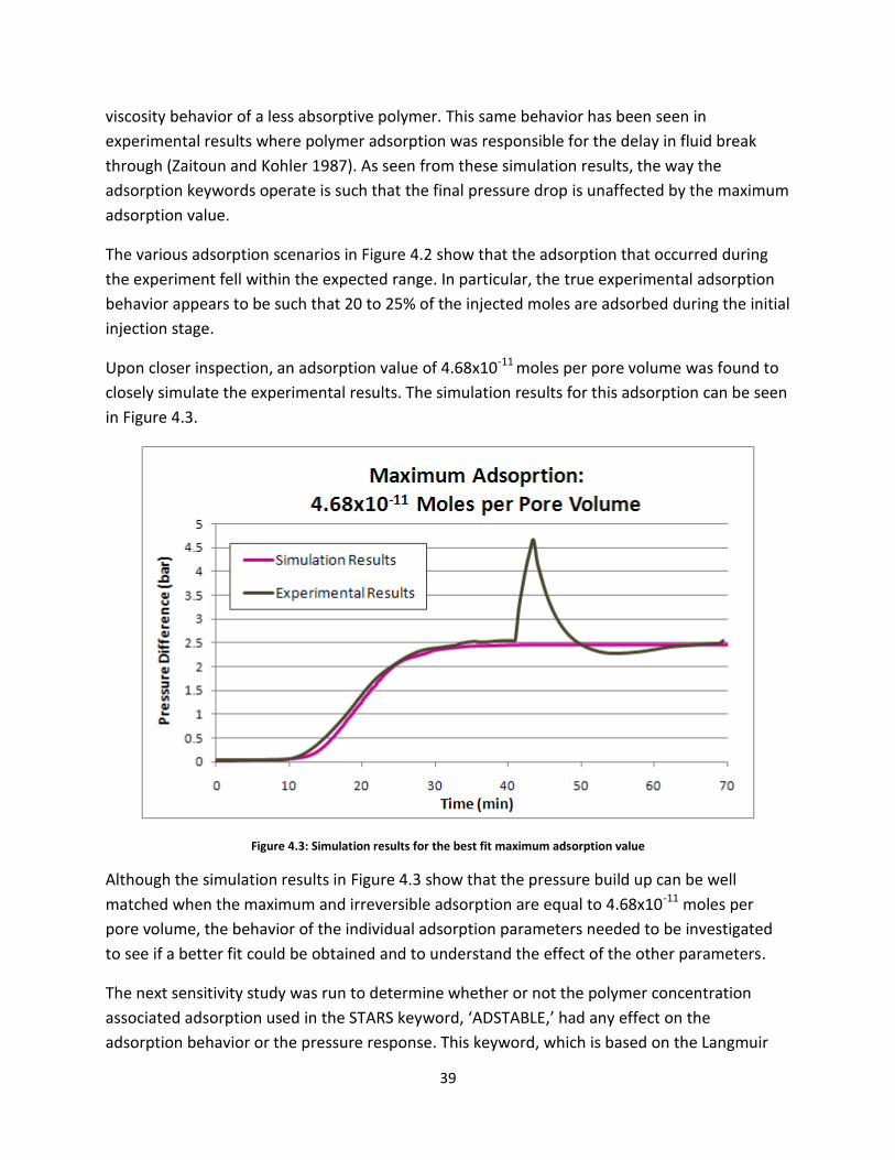
39

viscosity behavior of a less absorptive polymer. This same behavior has been seen in

experimental results where polymer adsorption was responsible for the delay in fluid break

through (Zaitoun and Kohler 1987). As seen from these simulation results, the way the

adsorption keywords operate is such that the final pressure drop is unaffected by the maximum

adsorption value.

The various adsorption scenarios in Figure 4.2 show that the adsorption that occurred during

the experiment fell within the expected range. In particular, the true experimental adsorption

behavior appears to be such that 20 to 25% of the injected moles are adsorbed during the initial

injection stage.

Upon closer inspection, an adsorption value of 4.68x10-11 moles per pore volume was found to

closely simulate the experimental results. The simulation results for this adsorption can be seen

in Figure 4.3.

Figure 4.3: Simulation results for the best fit maximum adsorption value

Although the simulation results in Figure 4.3 show that the pressure build up can be well

matched when the maximum and irreversible adsorption are equal to 4.68x10-11 moles per

pore volume, the behavior of the individual adsorption parameters needed to be investigated

to see if a better fit could be obtained and to understand the effect of the other parameters.

The next sensitivity study was run to determine whether or not the polymer concentration

associated adsorption used in the STARS keyword, ‘ADSTABLE,’ had any effect on the

adsorption behavior or the pressure response. This keyword, which is based on the Langmuir

40

isotherm, allows the user to input a table of polymer concentrations and associated adsorption

values. For this particular case, the adsorption value is associated with the injected polymer

concentration which, in units of mole fraction, is 1.87x10-9. As previously noted, this value

could not be lower than 1x10-10, and was therefore set as a constant in the previous sensitivity

study. Since the way the simulator handles adsorption is related to the amount of fluid being

injected, the limiting value in the adsorption table could be an issue for modeling small scale

situations such as a coreflood. In a reservoir scale situation however, this would not be

expected to be a problem since the volume of injected fluid, and therefore the number of

adsorbed moles of polymer would be significantly larger. Table 4.3 and Figure 4.4 display the

input parameters and corresponding results which were used to study the effect of the polymer

adsorption associated with the polymer concentration. The specific parameter that is being

varied in this case is the polymer adsorption (in units of moles per pore volume) that has been

input for the STARS keyword ‘ADSTABLE.’

Table 4.3: Input data for the Langmuir isotherm adsorption study - all adsorption parameters are in units of moles per pore volume

41

Figure 4.4: Simulation results for the study which investigated the effect of the keyword related to the Langmuir isotherm

As can be seen from the graph, despite the broad range of adsorption values that were

investigated in this study, all of the cases resulted in very similar pressure behavior. Since the

adsorption associated with the polymer concentration did not appear to affect the pressure

results, the original value of 1x10-10 was selected as the default for the rest of the sensitivity

studies.

In the two previous sensitivity studies, it was assumed that all of the adsorption was permanent

and irreversible. Since there was no experimental data to confirm whether this assumption was

correct or not, the irreversible adsorption was treated as a sensitivity parameter. Using a

maximum adsorption value of 4.68x10-11 moles per pore volume, the irreversible adsorption

was varied as a function of the maximum adsorption value from 75% to 95%. The input values

are presented in Table 4.4, where irreversible adsorption was studied in 5% increments. The

simulation results for each case are located in Figure 4.5.

42

Table 4.4: Input data for the irreversible adsorption study – all adsorption parameters are in units of moles per pore volume

Figure 4.5: Simulation results for the study which investigated the effect of the irreversible adsorption parameter

Just as varying the adsorption associated with the polymer concentration had no effect on the

pressure response, varying the irreversible adsorption as a function of the maximum adsorption

displayed a negligible effect. For the rest of the simulations, it was decided that it would suffice

to assume that all adsorption was permanent and irreversible.

The final sensitivity that was conducted for this flow rate investigated the effect of the

inaccessible pore volume. Until now, an inaccessible pore volume of 15% had been used in all of

the previous sensitivities. It was assumed that a range of reasonable inaccessible pore volume

values was somewhere between 10% and 20%. For the purpose of studying the simulators

behavior, this range was expanded to study inaccessible pore volumes ranging from 5% to 30%.

This study was conducted in increments of 5%. The input values and graphical results are

located in Table 4.5 and Figure 4.6, respectively.

43

Table 4.5: Input data for the inaccessible pore volume study - all adsorption parameters are in units of moles per pore volume

Figure 4.6: Simulation results for the study which investigated the effect of the inaccessible pore volume

From the graphical results it becomes apparent that the inaccessible pore volume does affect

the pressure behavior. Although the magnitude of the effect is smaller, increasing the

inaccessible pore volume affects the pressure results in a similar manner as decreasing the

maximum adsorption. The pressure drop in the core is able to build faster as the percentage of

the pore volume through which fluids are able to flow decreases. Although increasing or

decreasing the available pore volume affects the pressure build, it does not affect the stabilized

pressure result. From graphical observation it was determined that Case 3 represented the

experimental data the closest. This case was created using an inaccessible pore volume of 15%,

which falls within the expected range of inaccessible pore volumes and was therefore accepted

as a reasonable value.

44

The viscosity mixing function was also investigated for the 2 ml/min flow rate. This parameter

controls how quickly the maximum viscosity is achieved with relation to the polymer

concentration, so the fact that the viscosity mixing parameter affected the pressure build but

not the stabilized pressure difference is understandable. The results for three different cases

are displayed below. The first case represents an extreme situation where the ultimate viscosity

is achieved at very low polymer concentrations. The last case represents a linear mixing

function, and the middle case represents something in between the two extremes. As can be

seen, the pressure build can be manipulated to a decent extent by adjusting the mixing

function. Since the viscosity behavior of the polymer at lower concentrations was not known, a

linear mixing function was assumed.

Figure 4.6: Input data for the relationship between the polymer concentration and the viscosity behavior

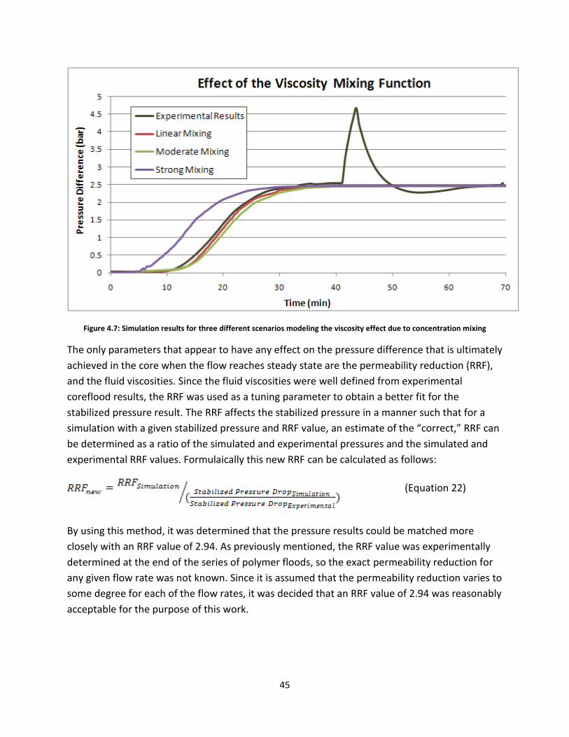
45

Figure 4.7: Simulation results for three different scenarios modeling the viscosity effect due to concentration mixing

The only parameters that appear to have any effect on the pressure difference that is ultimately

achieved in the core when the flow reaches steady state are the permeability reduction (RRF),

and the fluid viscosities. Since the fluid viscosities were well defined from experimental

coreflood results, the RRF was used as a tuning parameter to obtain a better fit for the

stabilized pressure result. The RRF affects the stabilized pressure in a manner such that for a

simulation with a given stabilized pressure and RRF value, an estimate of the “correct,” RRF can

be determined as a ratio of the simulated and experimental pressures and the simulated and

experimental RRF values. Formulaically this new RRF can be calculated as follows:

(Equation 22)

By using this method, it was determined that the pressure results could be matched more

closely with an RRF value of 2.94. As previously mentioned, the RRF value was experimentally

determined at the end of the series of polymer floods, so the exact permeability reduction for

any given flow rate was not known. Since it is assumed that the permeability reduction varies to

some degree for each of the flow rates, it was decided that an RRF value of 2.94 was reasonably

acceptable for the purpose of this work.

46

4.3.4 – PRESSURE MATCH FOR THE 2 ML/MIN FLOW RATE

After conducting the sensitivity studies to understand how the adsorption parameters affected

the simulated results, a final match was created for the 2 ml/min flow rate. Between the

inaccessible pore volume, the maximum adsorption, and the effect of polymer concentration

on the viscosity, there was a lot of flexibility in determining the values which provided the best

pressure match. Since none of these parameters were well defined from the experimental data,

the combination of the parameters was not well constrained. As a result, the values that were

selected to simulate the experimental pressure behavior do not create a unique match. It is not

hard to imagine that multiple combinations of values for the three aforementioned parameters

could result in simulated pressure differences that were well matched with the experimental

data. In a situation where the actual values for key parameters are not well known, it is

important to understand and experiment with a reasonable range of values for these

parameters. The input parameters and graphical results for the final match that was created are

presented below in Table 4.7 and Figure 4.8.

Table 4.7: Input parameters selected to model the first polymer injection rate - all adsorption parameters are in units of moles per pore volume

Figure 4.8: Simulation results displaying the accepted pressure match for the first injection rate

47

4.3.5 – PRESSURE MATCHES CREATED FOR THE OTHER FLOW RATES

After matching the first injection rate, the process of matching the other injection rates was just

a matter of adjusting the permeability reduction factor. The method that was used to

determine the appropriate permeability reduction value for the simulation was described

earlier in Equation 17. Since STARS does not allow for multiple values of RRF to be entered in a

single input file, a restart file had to be created for each new RRF value.

Problems pertaining to pressure instabilities were encountered as the flow rates increased. The

first injection rate that displayed these instabilities was the 6 ml/min injection rate. By

decreasing the time step associated with this injection rate it was possible to smooth out the

pressure fluctuations. The problem with the pressure fluctuations became more pronounced as

the injection rates increased to larger values, and it was not possible to dampen the instabilities

past an injection rate of 7.5 ml/min.

Multiple methods such as decreasing the size of the time step, increasing the number of

iterations, increasing the number of time cuts associated with changes in fluid saturations, and

increasing the maximum allowable number of time steps were tried to remedy this problem,

but they resulted in limited success beyond an injection rate of 7.5 ml/min. Because of this, it

was decided that all of the flow rates larger than 7.5 ml/min would be excluded from the

simulation. This meant that the decreasing injection rates, starting with the 3 ml/min rate,

would be simulated directly after the 7.5 ml/min injection rate.

48

4.3.6 – SINGLE PHASE SIMULATION RESULTS

The final pressure match which was created by reasonable manipulation of the RRF values for

the different injection rates is displayed in Figure 4.9.

Figure 4.9: Simulation results displaying the accepted pressure matches for all of the injection rates ranging from .02 mL/min to 7.5 mL/min

49

Additionally, since there were some issues encountered during the process of modeling the

higher injection rates, a zoomed-in version of these injection rates has been plotted in Figure

4.10. As can be seen from the ‘’Simulated Results,’’ line, despite the steps taken to reduce the

pressure fluctuations, the 7.5 mL/min flow rate still exhibits very minor oscillations.

Figure 4.10: A zoomed-in view of the well-matched results from the simulation for the increasing injection rates

50

The following table (Table 4.8) presents a summary of the results created by the simulation of

the single phase polymer flood. In this table, the final pressure differences across the second

core from the experimental and simulated data are compared for different flow rates.

Additionally, the RRF has been displayed for each flow rate along with the flow regime that

each flow rate was located in. The red font represents the increasing injection rates and the

blue font represents the decreasing injection rates.

Table 4.8: Summarized results from the simulation for the single phase polymer flood - red indicates increasing injection rate and blue indicates decreasing injection rate

Although the simulated data appears to fit the experimental data well from the graphs in Figure

4.9 and Figure 4.10, this does not seem to be the case when comparing the stabilized pressure

drop values. By viewing the results in this manner, it becomes immediately apparent that the

higher injection rates incurred a significantly larger amount of error than the lower flow rates.

Aside from any error associated with the pressure instabilities that occur at the higher flow

rates, there is also the possibility that errors were introduced in the pressure readings. When

conducting the multi-rate polymer floods the injection rates can take longer to stabilize than

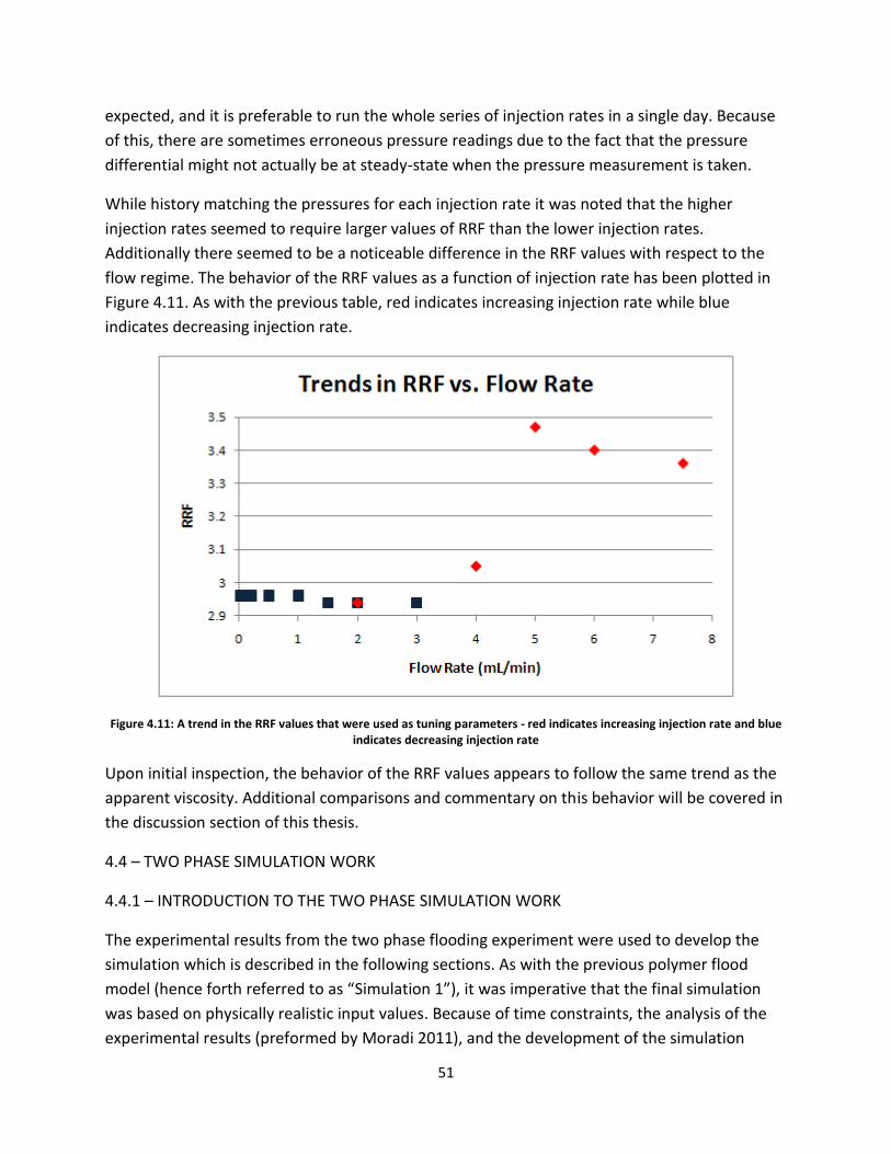
51

expected, and it is preferable to run the whole series of injection rates in a single day. Because

of this, there are sometimes erroneous pressure readings due to the fact that the pressure

differential might not actually be at steady-state when the pressure measurement is taken.

While history matching the pressures for each injection rate it was noted that the higher

injection rates seemed to require larger values of RRF than the lower injection rates.

Additionally there seemed to be a noticeable difference in the RRF values with respect to the

flow regime. The behavior of the RRF values as a function of injection rate has been plotted in

Figure 4.11. As with the previous table, red indicates increasing injection rate while blue

indicates decreasing injection rate.

Figure 4.11: A trend in the RRF values that were used as tuning parameters - red indicates increasing injection rate and blue indicates decreasing injection rate

Upon initial inspection, the behavior of the RRF values appears to follow the same trend as the

apparent viscosity. Additional comparisons and commentary on this behavior will be covered in

the discussion section of this thesis.

4.4 – TWO PHASE SIMULATION WORK

4.4.1 – INTRODUCTION TO THE TWO PHASE SIMULATION WORK

The experimental results from the two phase flooding experiment were used to develop the

simulation which is described in the following sections. As with the previous polymer flood

model (hence forth referred to as “Simulation 1”), it was imperative that the final simulation

was based on physically realistic input values. Because of time constraints, the analysis of the

experimental results (preformed by Moradi 2011), and the development of the simulation

52

model had to take place simultaneously. This resulted in a few parameters, which could have

been determined experimentally, being treated as uncertainties during the initial stages of the

simulation. These parameters included the apparent viscosity of the polymer during two phase

flow, the behavior of the relative permeability and saturation curves, and the adsorption

behavior. Since some of the analysis of the experimental results occurred independently from

the development of the simulation model, it was desirable to retrospectively confirm the

validity of the uncertain parameters if and where possible.

4.4.2 – MOBILE PHASE RELATIVE PERMEABILITY CURVE

Unlike Simulation 1 where the relative permeability curves were not a point of interest, it was

important to provide realistic relative permeability data for the two phase experiment. A

complete description of the permeability behavior as a function of the fluid saturation was not

available, but the end-point behavior was available as described in the experimental results for

the two phase polymer flood. Multiple scenarios with varying curvature were created to model

the relative permeability behavior. Once the curves were created, the most realistic looking

curves were tested in the simulator to see if they provided a good match with the experimental

data.

Since no visible oil production occurred for the first four injection rates, the oil relative

permeability was sufficiently accounted for with the proper end-point values. For these rates,

the shape of the curve between the oil related end-points was not of interest. Of course this

changed later when the injection rate was high enough that two phase flow occurred, at which

point the shape of the oil relative permeability curve became important. The most successful

water relative permeability behavior, as determined by the simulation results, is presented in

this section.

An initial approximation for the relative permeability behavior was created by fitting a straight

line through the water related end-point data. Because this sort of data tends to display more

curvature than is suggested by a straight-line model, additional variations with more curvature

were created. By manipulating the relative permeability value associated with the 41.85%

water saturation (which is half way between the interstitial and maximum water saturation), a

range of curves displaying more realistic shapes were produced. Since a linear trend is created

by setting the mid-point relative permeability to be equal to 50% of the maximum relative

permeability, curves with a concave-up trend were created by setting the mid-point value to be

between 10% and 40% of the maximum relative permeability. The numbers that were created

from this process are presented in Table 4.9. The data in the 50% column represents the data

associated with a straight line. The graphical results can be seen in Figure 4.12.

53

Table 4.9: Water relative permeability input data for varying cases of curvature

Figure 4.12: Multiple relative permeability scenarios developed by fitting a curve through the water relative permeability end-points

The “30% case” was selected for the simulation because it had a nice curvature and did not

contain any negative relative permeability values. The 10% and 20% cases were not presented

in the graph since they included unrealistic negative values. The curvature of the relative

permeability function was treated as a tuning parameter for the model, so any realistic starting

point was decidedly acceptable for the initial investigation.

54

4.4.3 – VISCOSITY BEHAVIOR IN THE POLYMER MIXING FRONT

From Simulation 1 it was understood that the primary polymer-related parameters which were

affecting how quickly the steady-state pressure difference was achieved were the maximum

adsorption, the effect of the polymer concentration on the solution viscosity, and the

inaccessible pore volume.

Bulk rheology experiments were conducted for multiple polymer concentrations, so the effect

of the polymer concentration on the solution viscosity was fairly well defined. Figure 4.13

displays the behavior of the polymer for concentrations varying from 0 to 2000 ppm. The

polymer concentration has been displayed in units of mole fractions rather than ppm since the

simulator required input units of mole fractions.

Figure 4.13: Non-linear behavior displayed in the relationship between viscosity and polymer concentration

As can be seen from the graph, the relationship between the polymer concentration and the

solution viscosity is not linear. The data set presented in Table 4.10 was calculated for polymer

concentrations ranging from 0 to 400 ppm from an equation that was created by fitting a

polynomial trend through the experimental data points. This data was then converted into the

form required by the simulator to account for the effects of non-linear mixing. A description of

the process required to convert the experimental data to simulation input values can be found

in the simulation manual (STARS Users Manual 2009).

55

Table 4.10: Polymer concentrations and associated solution viscosity values with non-linear behavior

The input values used to model the non-linear viscosity behavior due to polymer concentration

variations are shown in Table 4.11. The simulation default values, which correspond to linear

mixing behavior, are also presented in the table. As can be seen, the non-linear and the linear

values are not significantly different from each other. The plot in Figure 4.14, which displays

both data sets, further illustrates this point.

Table 4.11: Input data for the linear and non-linear viscosity mixing behavior based on polymer concentration

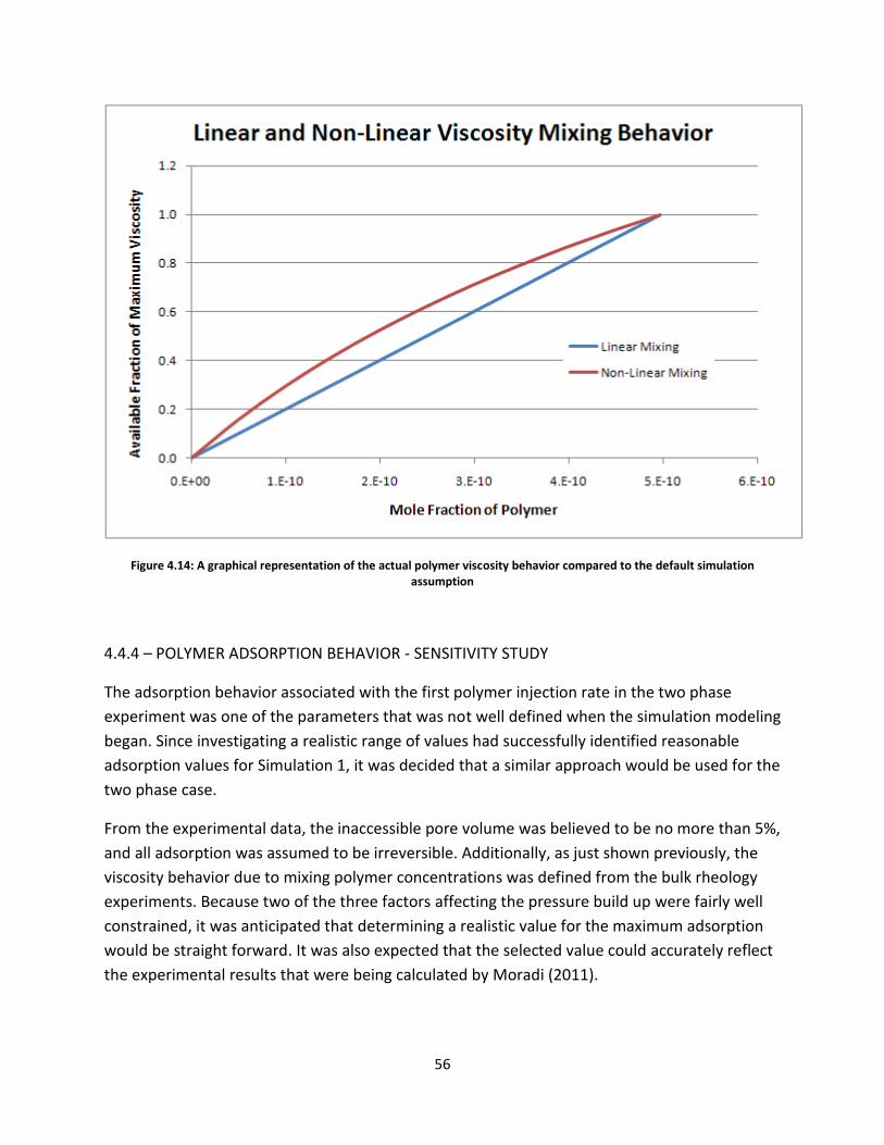
56

Figure 4.14: A graphical representation of the actual polymer viscosity behavior compared to the default simulation assumption

4.4.4 – POLYMER ADSORPTION BEHAVIOR - SENSITIVITY STUDY

The adsorption behavior associated with the first polymer injection rate in the two phase

experiment was one of the parameters that was not well defined when the simulation modeling

began. Since investigating a realistic range of values had successfully identified reasonable

adsorption values for Simulation 1, it was decided that a similar approach would be used for the

two phase case.

From the experimental data, the inaccessible pore volume was believed to be no more than 5%,

and all adsorption was assumed to be irreversible. Additionally, as just shown previously, the

viscosity behavior due to mixing polymer concentrations was defined from the bulk rheology

experiments. Because two of the three factors affecting the pressure build up were fairly well

constrained, it was anticipated that determining a realistic value for the maximum adsorption

would be straight forward. It was also expected that the selected value could accurately reflect

the experimental results that were being calculated by Moradi (2011).

57

Adsorption values ranging from 5% to 30% of the injected moles were investigated to identify

the adsorption behavior. An experimentally determined value of 1.3958 was used to account

for the permeability reduction (Moradi 2011). Since the apparent viscosity data was not

available for the 400 ppm polymer concentration, the viscosity of the polymer needed to be

determined before the sensitivity study could be run.

Given that the .2 mL/min injection rate resulted in single phase flow conditions, the apparent

viscosity could be estimated from the Darcy equation. Using the core dimensions, the steady-

state pressure difference, and the polymer relative permeability, an apparent viscosity of 1.75

cp was computed. With the polymer viscosity determined, all of the necessary inputs were

accounted for and the sensitivity could be preformed. The input values used for the maximum

adsorption study and the associated simulation results are presented respectively in Table 4.12

and Figure 4.15.

Table 4.12: Input values for the two phase maximum adsorption study

Figure 4.15: Differential pressures determined by the simulator for a range of maximum adsorption values for the two phase simulation - all adsorption parameters are in units of moles per pore volume

58

As can be seen, a maximum adsorption of 15% provided the best fit for the experimental

results. Because the 15% case provided the best fit and seemed like a reasonable value, it was

accepted as the maximum adsorption value for the simulation model.

Despite the multitude of efforts taken to achieve a better match via investigating the other

simulation parameters, the experimental pressure data that was recorded before

approximately 90 minutes could not be matched. Upon closer inspection it was noticed that the

slope of the pressure build-up changes around 90 minutes. The nature of the experimental

process, and the uncertainty associated with different pieces of equipment is such that it is not

uncommon for sections of data to be neglected with reasonable cause. Since there was an

unexpected change in the rate of the pressure build, and the pressure spike at the beginning of

the data seemed incorrect, it was suspected that something went awry with the pumping

system at the beginning of the polymer injection.

4.4.5 – PRESSURE MATCH FOR THE FIRST INJECTION RATE

As was the case with Simulation 1, creating a good match which used realistic values was

considered a priority for the first polymer injection rate. Although there was some uncertainty

surrounding the behavior of the initial data, the simulation results fit the experimental results

quite well after 90 minutes. Since the inputs used in the simulation model were largely based

on experimentally derived values or ranges of values, the simulation results were decidedly

good enough to begin focusing on the other injection rates. The finalized simulation model for

the first injection rate used a maximum adsorption of 15%, a water relative permeability curve

that corresponded to the 30% curvature case, and an apparent viscosity value of 1.75 cp. By

using these simulation-derived parameters along with the experimentally derived parameters,

the pressure match displayed in Figure 4.16 was created.

Table 4.16: Differential pressure match for the first injection rate in the two phase simulation

59

4.4.6 – POLYMER APPARENT VISCOSITY VALUES FOR VARIOUS SINGLE PHASE FLOW RATES

The three injection rates that followed the initial injection rate also resulted in single phase

flow. Assuming that the adsorption behavior related to the initial injection rate was modeled

correctly, the apparent viscosity of the polymer was the only unknown parameter for each of

these flow rates. As before, the Darcy equation was applicable, as were the previously used

core dimensions and permeability values. Using these parameters, the following apparent

viscosity values were determined. The Darcy velocity is included in the table because the

apparent viscosity is associated with the Darcy velocity rather than the injection rate in the

simulator.

Table 4.13: Viscosity input data for the single phase flow rates

4.4.7 – INPUT DATA FOR TWO PHASE FLOW

Estimating the apparent viscosity is a straight forward procedure for single phase flow, but it

becomes more complicated when two flowing phases are present. As the injection rate was

increased from 1.6 mL/min to 3.2 mL/min, oil was produced along with the polymer indicating

the presence of two phase flow. This meant that the Darcy-based method which was previously

used to calculate the apparent viscosity would no longer work since there were too many

unknowns. Instead, a basic understanding of how the apparent viscosity transitioned from one

regime to another was used to create an estimate that was then refined by adjustments which

were decided upon by multiple simulations.

60

The process to determine the apparent viscosity began by plotting the data from Table 4.13 as

a function of the injection rate to see what the trend looked like. The graphical result from this

is displayed below in Figure 4.17.

Figure 4.17: Darcy-based apparent viscosity values for the single phase flow rates of the two phase experiment

By presenting the viscosity data on a semi-log plot, as was done here, it becomes apparent that

the three largest rates fall in the shear thickening regime.

The maximum achievable apparent viscosity was unknown, so it was not immediately obvious

whether the 3.2 mL/min rate was in the shear thickening or the degradation regime. To

determine this required running some scenarios in the simulator for representative values and

observing the results. It was suspected that the injection rate of 3.2 mL/min would continue to

reflect shear thickening behavior. Either way, the range of expected behavior was narrowed by

understanding the realm of possible behavior based on the flow regimes.

Since a continuation of the shear thickening regime seemed most probable, a polynomial trend

line was fit through the data and used to extrapolate the apparent viscosity for the rate of 3.2

mL/min. The graphical result of this process can be seen in Figure 4.18. The orange line

represents the apparent viscosity model that was created for use in the simulator, and the

purple points represent the apparent viscosity values that were calculated for the first four

injection rates.

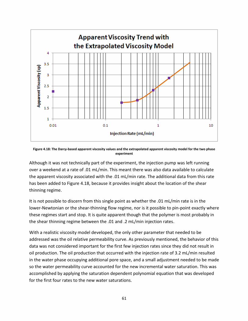
61

Figure 4.18: The Darcy-based apparent viscosity values and the extrapolated apparent viscosity model for the two phase experiment

Although it was not technically part of the experiment, the injection pump was left running

over a weekend at a rate of .01 mL/min. This meant there was also data available to calculate

the apparent viscosity associated with the .01 mL/min rate. The additional data from this rate

has been added to Figure 4.18, because it provides insight about the location of the shear

thinning regime.

It is not possible to discern from this single point as whether the .01 mL/min rate is in the

lower-Newtonian or the shear-thinning flow regime, nor is it possible to pin-point exactly where

these regimes start and stop. It is quite apparent though that the polymer is most probably in

the shear thinning regime between the .01 and .2 mL/min injection rates.

With a realistic viscosity model developed, the only other parameter that needed to be

addressed was the oil relative permeability curve. As previously mentioned, the behavior of this

data was not considered important for the first few injection rates since they did not result in

oil production. The oil production that occurred with the injection rate of 3.2 mL/min resulted

in the water phase occupying additional pore space, and a small adjustment needed to be made

so the water permeability curve accounted for the new incremental water saturation. This was

accomplished by applying the saturation dependent polynomial equation that was developed

for the first four rates to the new water saturations.

62

The same procedure which was used to create the water relative permeability curve was

followed to create the oil relative permeability curve. As before, the initial curve was

approximated by a straight line fit through the end-point data. The shape of the data was then

manipulated by multiplying factors which varied from 10% to 40%. In this process, the oil

relative permeability associated with the mid-point saturation, which controlled the curvature

of each case, was calculated by multiplying the maximum possible oil relative permeability by

these percentages. The values that were created from this procedure are presented in Table

4.14 and plotted in Figure 4.19.

Table 4.14: Oil relative permeability input data for varying cases of curvature

Figure 4.19: Multiple relative permeability scenarios developed by fitting a curve through the oil relative permeability end-points

Again, the 30% case was selected to be used in the simulator. Again, the 10% and 20% cases are

not presented in the graph since they resulted in unrealistic negative values. Because the

relative permeability curves for the first four injection rates differed from the relative

permeability curve for the last injection rate that was simulated, a restart file was used. Other

63

than the adjustments to the injection rate, the relative permeability behavior was the only

difference between the two files.

Ultimately, the data that was input in the simulator for both the oil and water relative

permeability values used the 30% cases. The calculated curves were based on the end-point

values from the 3.2 mL/min injection rate. These curves were then adjusted for use with the

single phase flow injection rates by setting the end-points to properly reflect the experimental

data. The water saturations and associated relative permeability values for each of the files are

presented below in Table 4.15 and Table 4.16. The values used to model the two phase flow

situation are also presented in graphical form in Figure 4.20.

Table 4.15: Finalized relative permeability and saturation values for the single phase rates

64

Table 4.16: Finalized relative permeability and saturation values for the two phase rate

Figure 4.20: The relative permeability model for the oil and water phases

With the relative permeability behavior modeled, all of the required input parameters were

accounted for and the simulation model was ready to be run and evaluated.

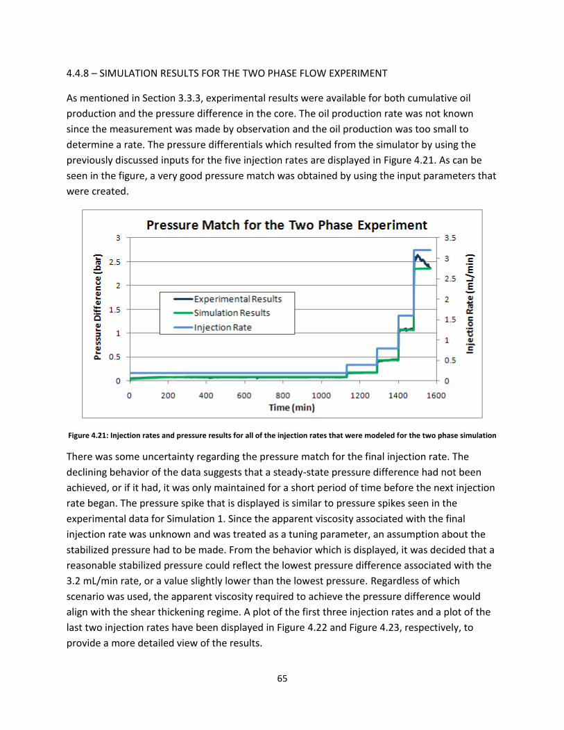
65

4.4.8 – SIMULATION RESULTS FOR THE TWO PHASE FLOW EXPERIMENT

As mentioned in Section 3.3.3, experimental results were available for both cumulative oil

production and the pressure difference in the core. The oil production rate was not known

since the measurement was made by observation and the oil production was too small to

determine a rate. The pressure differentials which resulted from the simulator by using the

previously discussed inputs for the five injection rates are displayed in Figure 4.21. As can be

seen in the figure, a very good pressure match was obtained by using the input parameters that

were created.

Figure 4.21: Injection rates and pressure results for all of the injection rates that were modeled for the two phase simulation

There was some uncertainty regarding the pressure match for the final injection rate. The

declining behavior of the data suggests that a steady-state pressure difference had not been

achieved, or if it had, it was only maintained for a short period of time before the next injection

rate began. The pressure spike that is displayed is similar to pressure spikes seen in the

experimental data for Simulation 1. Since the apparent viscosity associated with the final

injection rate was unknown and was treated as a tuning parameter, an assumption about the

stabilized pressure had to be made. From the behavior which is displayed, it was decided that a

reasonable stabilized pressure could reflect the lowest pressure difference associated with the

3.2 mL/min rate, or a value slightly lower than the lowest pressure. Regardless of which

scenario was used, the apparent viscosity required to achieve the pressure difference would

align with the shear thickening regime. A plot of the first three injection rates and a plot of the

last two injection rates have been displayed in Figure 4.22 and Figure 4.23, respectively, to

provide a more detailed view of the results.

66

Figure 4.22: Injection rates and pressure results for the lower injection rates that were modeled for the two phase simulation

Figure 4.23: Injection rates and pressure results for the higher injection rates that were modeled for the two phase simulation

The simulation resulted in a cumulative oil production of 1.087 mL which was found to closely

match the experimental value of 1.1 mL. The error between these two values was only 1.12%,

so the cumulative production was considered to be well matched. As can be seen in the

graphical results in Figure 2.24, the oil production begins immediately after the injection rate is

increased from 1.6 mL/min to 3.2 mL/min. Once the oil production starts, it appears to occur

67

quite rapidly in a manner that would result from piston-like displacement. Figure 4.25 gives a

more detailed view of the cumulative oil production along with the oil production rate.

Figure 4.24: Simulated cumulative oil production for the injection rates up to 3.2 mL/min

Figure 4.25: A zoomed-in view of the cumulative oil production and oil production rate with the experimental production plotted for comparison

68

CHAPTER 5 - DISCUSSION

5.1 – SINGLE-PHASE POLYMER FLOOD

From the presented results, it appears that the CMG STARS simulator is capable of modeling

the pressure behavior associated with a high molecular weight polymer flood operated under a

broad range of injection rates. By manipulating some of the more flexible parameters with in a

realistic range, the experimental pressure results for multiple injection rates were well-matched

pressure using Simulation 1. Although the initial pressure spikes exhibited in the experimental

data were not matched by the simulator, the agreement between the experimental and

simulated results were still very good. As previously mentioned, the pressure spikes were

probably due to polymer alignment or polymer degradation at the front of the core, and it was

not anticipated that the simulator would be able to model this behavior. Two points of interest

were identified while working with Simulation 1, the first of which had to do with the pressure

instabilities that occurred at the higher injection rates. All of the methods typically used to

dampen the fluctuations were used but were not successful for injection rates above 7.5

mL/min.

For the purpose of simulating a field-scale polymer injection process, the pressure instabilities

associated with high flow rates probably would not be an issue. The high rates which were

tested in the laboratory experiment are typically studied to see the range of a polymers

behavior, but are rarely implemented in the field. While that is good news with respect to the

field application, it is less than preferable for modeling high rates in the lab.

This leads into point number two which has to do with variation in the RRF value as a function

of injection rate. As previously described, the RRF value was used as a tuning parameter to

match the steady-state pressure differences of the individual flow rates. Simulating the larger

flow rates resulted in pressure fluctuations, so it was not possible to determine an RRF value for

these flow rates. The behavior of the RRF values as a function of flow rate displayed a trend

very similar to that of the apparent viscosity and RF values. Whether or not there is any physical

reason to believe that the RRF values actually follow this sort of trend is something that

requires further investigation.

The apparent viscosity values that were used in the previously presented simulation model

were calculated by assuming a constant RRF value of 3.6. Aside from being used to determine

the apparent viscosity, the RRF value was also accounted for in the adsorption parameters.

When history matching the pressure differences, the RRF value associated with the adsorption

parameters was changed while the one used to calculate the apparent viscosity was held

constant. Since the steady-state pressure drop is affected by all of the parameters included in

69

the Darcy equation, the RRF adjustments could be making up for any minor errors associated

with the other parameters.

Alternatively, the trend of the manipulated RRF values could have a physical basis since it has

been suggested that the RRF could vary with flow rate (Chauveteau et al. 2002). Either way,

results from a singular simulation cannot definitively prove this behavior, so this could be a

subject of future investigations.

The plot displayed in Figure 5.1, shows the resulting pressure match for the situation where the

RRF was held at a constant value of 3.6 instead of being treated as a tuning parameter. Since

plotting all of the injection rates on a single plot makes it hard to see the discrepancies in the

data, only the increasing injection rates are shown.

Figure 5.1: Simulated differential pressure results with a constant RRF of 3.6

As can be seen, by holding the RRF at a constant value of 3.6, the steady-state pressure

difference is consistently overestimated.

5.2 – TWO-PHASE POLYMER FLOOD

By using experimentally derived input values and realistic ranges of input values for the

parameters which were uncertain, a simulation model that matched both pressure and

cumulative production data was created. The shape of the relative permeability curves, and the

apparent viscosity associated with the different injection rates were among the parameters

that carried some uncertainty. Since there was not any data available to model the rate at

which the oil was produced, the importance of tuning the relative permeability curves had less

to do with manipulating the finer details of the curves to ensure an oil rate was matched and

70

more to do with ensuring that the cumulative oil production was correct for a given flow rate.

Additionally, the state of the fluid saturations in both the simulator and the experiments could

be accounted for by a fairly narrow range of values on the relative permeability curves, so those

were the primary focus of manipulation rather than the whole curve. Once the relative

permeability values were correct for the range of interest, the remainder of the curve was

structured to incorporate the range of interest in a seamless manner.

The apparent viscosity table that is used for modeling the polymer viscosity behavior plays a

significant role in determining the steady-state pressure difference. Since values were not

directly available to model this behavior, the apparent viscosity values were determined from

the Darcy equation and an extrapolation method. The values that were used in the model were

ultimately selected because they created simulation results that were well matched with the

experimental results. This is especially true for the apparent viscosity associated with the last

injection rate which was chosen based on a combination of trend-line extrapolation and “guess-

and-check,” style simulation trials.

From the experimental work conducted by Stavland et al. (2010), there happened to be

apparent viscosity data available for the same polymer type that was used in the two phase

injection model but at a concentration of 600 ppm instead of 400 ppm. It was decided that an

observational comparison of the apparent viscosity values associated with each of the polymer

concentrations could provide more insight about the accuracy of the apparent viscosity values

created for the 400 ppm polymer. Figure 5.2 displays the apparent viscosity values of the two

polymer concentrations as a function of shear rate. In both cases, the conversion between the

flow rate and the shear rate was calculated using the absolute permeability.

71

Figure 5.2: Flow regime related transitions and trends in apparent viscosity values for a 400 ppm and a 600 ppm polymer

From the graph it can be seen that while the apparent viscosity for the 600 ppm polymer

appears to reach a larger value, the 400 ppm polymer has not yet achieved its maximum

viscosity value for the given range of shear rates. It also appears that the 400 ppm polymer

transitions to the shear thickening regime for values of shear rate which the 600 ppm polymer

is exhibiting shear thinning behavior. This situation seems unrealistic since it is generally

expected that, for a given polymer type, the solutions with higher concentrations will not only

achieve larger apparent viscosity values but they will also go through the sequence of flow

regimes at lower shear rates than the lower concentrations will (Heemskerk et al. 1984). The

apparent viscosity behavior displayed in Figure 5.3 for concentrations of 1500 and 600 ppm

graphically exemplifies this statement. Again, the polymer type is the same for both solutions,

but the concentrations are different.

72

Figure 5.3: Flow regime related transitions and trends in apparent viscosity values for a 600 ppm and a 1500 ppm polymer

Another similarity between these two polymers is that both were injected into 100% water

saturated cores. The 400 ppm polymer solution was injected into a core which contained

residual oil saturation with the remaining saturation being taken up by water. In addition to the

permeability effects due to polymer adsorption, which all of the core flood experienced after

polymer injection had taken place, the 400 ppm polymer had another factor affecting the

permeability. Before the 400 ppm polymer was injected into the core, it had already been

affected by residual oil. In turn, the core had already had developed a permeability scenario

that deviated from the absolute permeability before the polymer was injected.

Since the polymer cannot flow in the space occupied by the residual oil, it was decided to adjust

the shear rate according to the relative permeability effect from the residual oil. The relative

permeability value that was used did not take into account the polymer adsorption effects, so it

was believed that using this relative permeability for the case with residual oil saturation would

be analogous to using the absolute permeability for the 100% water saturated scenarios.

Figure 5.4 displays the results that were acquired from using this relative permeability to adjust

the shear rate of the 400 ppm polymer.

73

Figure 5.4: “Properly aligned” flow regime transitions and trends for a 400 ppm and a 600 ppm polymer

The locations and development of the flow regimes for the 400 ppm and 600 ppm polymer

concentrations presented in this graph reflect the expected behavior much more closely than

the previous graph. This could indicate that for the purpose of correlating shear rate values

with flow rate values, when residual oil is present, the permeability effects associated with the

oil will need to be accounted for. Since this assessment is based on a data set consisting of only

one experiment, more investigations will be required before any concrete statements can be

made.

Another factor that is at play in this situation is the fact that the 600 ppm flood was conducted

in a Berea sandstone core while the 400 ppm flood was conducted in a Bentheim sandstone

core. An alpha value of 2.5 was used in the shear rate conversion for the Berea sandstone core.

Whether or not there was any physical basis to do so, this same alpha value was also used for

the Bentheim sandstone core. If an alpha value of 2.5 is physically inaccurate for the Bentheim

sandstone core, then this will also affect the flow rate to shear rate conversion. While it was

considered important to mention this point for the sake of completeness, no further work was

done with regards to the alpha factor.

74

CHAPTER 6 – SUMMARY, CONCLUSIONS AND RECCOMMENDATIONS

6.1 – SINGLE-PHASE SIMULATION MODELING

By utilizing the polymer-related simulation capabilities which are currently available in the

simulation software, CMG STARS, two sets of experimental data have been modeled and

matched using physically realistic input parameters. The first experiment consisted of a single

phase polymer injection with injection rates varying from .02 mL/min to 20 mL/min. Within this

range of injection rates, the polymer fluid exhibited at least shear thinning, shear thickening,

and degradation behavior. Experimental data was used to create a table of velocity and

associated viscosity values which accurately described the polymers behavior. Although

adsorption data was not available, a sensitivity study preformed for a reasonable range of

values was found to be a successful tool for identifying the related adsorption behavior. This

study was also useful for gaining a better understanding of how the adsorption model

embedded in the simulator could be used to model polymer floods in the core scale (and

potentially the field scale). For this portion of the work, the experimental pressure differential

in the second core was the available data which was to be matched.

Of the available injection rates, the largest rate successfully modeled was the 7.5 mL/min rate

which corresponded to the degradation regime. Other injection rates which exhibited

degradation behavior and were also successfully modeled include the 4 mL/min, 5 mL/min, and

6 mL/min rates. It was of particular interest to model the degradation regime, since previously

only up to the shear thickening regime had been successfully simulated. Injection rates larger

than 7.5 mL/min were not successfully modeled because of the large pressure fluctuations that

were produced in the simulator despite attempts to dampen them. It is important to note that

the shear thickening and degradation behaviors occur at very high flow rates which rarely if

ever occur in the reservoir (Seright 2010). Instead, these high rates, and their associated flow

regimes are most likely to be encountered in the near wellbore area, especially in the vicinity of

the injection well. All of the injection rates below 5 mL/min were simulated without any

problems.

By using the permeability reduction (RRF) value as a tuning parameter, a well matched pressure

fit was created. When plotted against flow rate, the permeability reduction values used to

match the simulated and experimental pressures created a trend very similar to the one

displayed by the apparent viscosity and the mobility reduction. Whether this trend actually

reflects a physical characteristic of the permeability reduction is something that can be

investigated in further studies.

75

6.2 – TWO-PHASE SIMULATION MODELING

The two phase experiments consisted of injecting a polymer solution into a single core with

residual oil saturation. As the injection rates increased above 3.2 mL/min, some of the oil that

was previously considered residual oil was produced which resulted in a decrease in the

residual oil saturation and an increase in the water phase saturation. The two phase

experiment was conducted for injection rates ranging from .2 mL/min to 18 mL/min. For this

work only the rates ranging from .2 mL/min to 3.2 mL/min were simulated. The rate at which

two phase flow occurred was of particular interest for this work. Of the rates studied, the 3.2

mL/min injection rate produced 1.1 mL of oil while the lower rates resulted in single phase flow.

Since the availability of experimentally derived adsorption values which could be directly

applied to the simulation model was sparse, a sensitivity study was conducted to determine the

adsorption behavior. As with the single phase simulation model, conducting a sensitivity study

proved to be a successful method for identifying realistic adsorption behavior. Relative

permeability curves were constructed based on experimentally derived end-point data. The

apparent viscosity behavior was not as defined as it had been for the single phase model. To

remedy this, the Darcy equation was implemented for the injection rates that resulted in single

phase flow. The apparent viscosity for the injection rate associated with two phase flow was

extrapolated by fitting a line through the previously calculated values. It was assumed that the

behavior of the unknown apparent viscosity was a continuation of the shear thickening regime,

so the options for the extrapolated value were constrained to reflect this assumption. A single

experimentally-determined RRF value was used for all of the injection rates which were

studied. From the bulk rheology data, an understanding of the frontal mixing behavior was

developed and implemented in the simulator. After making minor adjustments to the curvature

of the relative permeability behavior as well as minor adjustments to the apparent viscosity

associated with the injection rate of 3.2 mL/min, a simulation model was created which

matched both the experimental pressure differential and the cumulative oil production of 1.1

mL.

Experimentally derived apparent viscosity results were available for a 600 ppm polymer

solution which utilized the same polymer as the one that was simulated. Because the apparent

viscosity values that were used in the simulation were developed by the Darcy equation and an

educated extrapolation, it was of interest to compare these values with other related data to

see if they corroborated.

It was possible to confirm that the apparent viscosity behavior which was developed for the

simulation model was realistic by comparing it with the 600 ppm data. While preparing the two

data sets for comparison, an observation was made regarding the velocity to shear rate

conversion for the two phase data. A misalignment of the 400 ppm flow regimes relative to the

76

600 ppm flow regimes called to question whether using the absolute permeability value was

appropriate for the two phase case. After recalculating the shear rate using the relative

permeability value that accounted for the presence of residual saturations, the flow regimes

aligned in the expected manner. Whether or not it is physically correct to replace the absolute

permeability with the relative permeability in this manner is a topic which can be investigated

in further studies.

77

NOMENCLATURE

= Upper Newtonian Viscosity, cp

= Lower Newtonian Viscosity, cp

= Viscosity, cp

= Shear Rate, 1/s

n = Shear Thinning Exponent, dimensionless

= Shear Rate at the Lower Newtonian-Shear Thinning Boundary, 1/s

n = Shear Thinning Exponent

= Stretch Rate, s

= Interstitial Velocity, m/s

= Average Grain Diameter, m

k = Permeability, mD

= Porosity, fraction

= Formation Tortuosity

= Deborah Number, dimensionless

= Relaxation Time, s

= Elongation Viscosity, cp

= Maximum Viscosity, cp

= Shear Thickening Viscosity, cp

m = Elongation Exponent, dimensionless

= Critical Shear Rate for Shear Thickening, s

= Newtonian Viscosity of the Effluent, cp

= Viscosity at Zero Shear Rate, cp

= Critical Shear Rate for Degradation, s

k = Shear Thinning Exponent for Degradation Model

x = Tuning Parameter for the Degradation Model

78

= Polymer Intrinsic Viscosity, cp

= Molecular Weight, Dalton

= Gyration Radius, m

= Universal Constant Equal to 4.2x1024

A = Cross Sectional Area, m2

r = Pore Radius, m

d = Thickness Close to the Wall (Associated with Polymer Thickness), m

IPV = Inaccessible Pore Volume

B = Constant that Controls the Apparent Viscosity at Low Shear Rates

RF = Mobility Reduction

RRF = Permeability Reduction

= Experimentally Determined Apparent Viscosity, cp

= Tuning Parameter Associated with the Rock Particles

= Apparent Viscosity Determined from the Model by Stavland et al. 2010, cp

= Water Viscosity, cp

= Apparent Viscosity at Zero Shear Rate, cp

j = Tuning Parameter

79

REFERENCES

1.) Chauveteau, G., Denys, K. and Zaitoun, A. 2002. New Insight on Polymer Adsorption Under High Flow

Rates. Paper SPE 75183, presented at the SPE/DOE Improved Oil Recovery Symposium, Tulsa, Oklahoma,

U.S.A., 13-17 April. DOI: 10.2118/75183-MS.

2.) Delshad, M., Kim, D. H., Magbagbeola, O. A., Huh, C., Pope, G. A. and Tarahhom, F. 2008. Mechanistic

Interpretation and Utilization of Viscoelastic Behavior of Polymer Solutions for Improved Polymer-Flood

Efficiency. Paper SPE 113620, presented at the SPE/DOE Improved Oil Recovery Symposium held in

Tulsa, Oklahoma, U.S.A., 19-23 April. DOI: 10.2118/113620-MS.

3.) Green, D. W. and Willhite, G. P. 1998. Enhanced Oil Recovery. Henry L. Doherty Memorial Fund of AIME,

Society of Petroleum Engineers.

4.) Heemskerk, J., Janssen-van Rosmalen, R., Holtslag, R. J. and Teeuw, D. 1984. Quantification of

Viscoelastic Effects of Polyacrylamide Solutions. Paper SPE/DOE 12652, presented at the SPE/DOE

Symposium on Enhanced Oil Recovery, Tulsa, Oklahoma, 15-18 April. DOI: 10.2118/12652-MS.

5.) Hirasaki, G. J. and Pope, G. A. 1974. Analysis of Factors Influencing Mobility and Adsorption in the Flow

of Polymer Solution through Porous Media. SPE Journal, 337-346, Aug. 1974. DOI: 10.2118/4026-PA.

6.) Moradi, H. 2011. Experimental Investigation of Polymer Flow through Water- and Oil-Wet Porous Media,

Thesis, University of Stavanger.

7.) Maerker, J. M. 1975. Shear Degradation of Partially Hydrolyzed Polyacrylamide Solutions. SPE Journal,

311-322, Aug. 1975. DOI: 10.2118/5101-PA.

8.) Maerker, J. M. 1976. Mechanical Degradation of Partially Hydrolyzed Polyacrylamide Solutions in

Unconsolidated Porous Media. SPE Journal, 172-174, Aug 1976. DOI: 10.2118/5672.

9.) Masuda, Y., Tang, K., Miyazawa, M. and Tanaka, S. 1992. 1D Simulation of Polymer Flooding Including

the Viscoelastic Effect of Polymer Solution, SPE Reservoir Engineer, 247-252, May 1992. DOI:

10.2118/19499-PA.

10.) Morris, C. W. 1978. Mechanical Degradation of Polyacrylamide Solutions in Porous Media. Paper SPE

7064, presented at the SPE Symposium on Improved Methods of Oil Recovery, Tulsa, Oklahoma, U.S.A.,

16-17 April 1978. DOI: 10.2118/7064-MS.

11.) Seright, R. S. 1983. The Effects of Mechanical Degradation and Viscoelastic Behavior on Injectivity of

Polyacrylamide Solutions. SPE Journal, 475-485, June 1983. DOI: 10.2118/9297-PA.

12.) Seright, R. S., Fan, T., Wavrik, K., Balaban, R. 2010. New Insights into Polymer Rheology in Porous Media.

Paper SPE 129200, presented at the 2010 SPE Improved Oil Recovery Symposium, Tulsa, Oklahoma,

U.S.A, 24-28 April 2010. DOI: 10.2118/129200-MS.

13.) Sorbie, K. S. 1991. Polymer-Improved Oil Recovery. Glasgow, Scotland: Blackie and Sons Ltd.

14.) Southwick, J. G. and Manke, C. W. 1988. Molecular Degradation, Injectivity, and Elastic Properties of

Polymer Solutions. SPE Journal, 1193-1201, November 1988. DOI: 10.2118/15652-PA.

15.) STARS Users Manual, Version 2009.13, Computer Modeling Group, Calgary, Alberta, Canada, 2009.

16.) Stavland, A., Jonsbraaten, H.C. and Lohne, A. 2010. Polymer Flooding – Flow Properties in Porous Media

versus Rheological Parameters. Paper SPE 131103, presented at the SPE EUROPE/EAGE Annual

Conference and Exhibition, Barcelona, Spain 14-17 June 2010. DOI: 10.2118/131103-MS.

80

17.) Zaitoun, A. and Kohler, N. 1987. The Role of Adsorption in Polymer Propagation through Reservoir

Rocks. Paper SPE 16274, presented at the SPE International Symposium on Oilfield Chemistry, San

Antonio, Texas 4-6 February 1987. DOI: 10.2118/16274-MS.

18.) Zaitoun, A. and Chauveteau, G. 1998. Effect of Pore Structure and Residual Oil on Polymer Bridging

Adsorption. Paper SPE 39674, presented at SPE/DOE Improved Oil Recovery Symposium, Tulsa,

Oklahoma, U.S.A. 19-22 April 1998. DOI: 10.2118/39674-MS.

19.) Zitha, P., Chauveteau, G., Zaitoun, A. 1995. Permeability-Dependent Propagation of Polyacrylamides

under Near-Wellbore Flow Conditions. Paper SPE 28955, presented at the SPE International Symposium

on Oilfield Chemistry, San Antonio, Texas, 14-17 February 1995. DOI: 10.2118/28955-MS.