CoreMathTools

Link to help topics (below) by Mathematics Strand, Tool, or Feature ornavigate the Help PDF (choose Info | PDF from the main tools page):

Do a "search" using the "Find" feature (control+F);View the navigation pane within your PDF viewer ("side bar,""bookmarks bar," or "drawer");Click on section headers within the navigation pane, scroll throughpages, use up and down arrows; orReference the Site Map for a linked outline of all help content.

Algebra & Functions Geometry &Trigonometry

Statistics & Probability

CAS

Graphs & Tables

Symbolic Manipulation

Synthetic

Draw & Measure

Construct & Transform

Data Analysis

Graphical Display

Statistical Analysis

Spreadsheet

Formulas

Data Sort

Coordinate

Program & Animate

Geometry Commands

Simulation

Build & Run

View & Analyze

Custom Apps Custom Apps Custom Apps

Quick LinksCatalog Index Save & Print Advanced Apps

CoreMathTools

www.nctm.org/coremathtools

Core Math Tools is a suite of Algebra & Functions, Geometry & Trigonometry,and Statistics & Probability software tools designed to support implementation ofthe Common Core State Standards for Mathematics.

Core Math Tools includes three families of software:

Algebra & Functions—The software for work on algebra problems includes an electronicspreadsheet and a computer algebra system (CAS) that produces tables and graphs of functions,manipulates algebraic expressions, and solves equations and inequalities.

Geometry & Trigonometry—The software for work on geometry problems includes an interactivedrawing program for constructing, measuring, and manipulating geometric figures and a set ofcustom apps for exploring properties of two- and three-dimensional figures.

Statistics & Probability—The software for work on data analysis and probability problemsprovides tools for graphic display and analysis of data, simulation of probabilistic situations, andmathematical modeling of quantitative relationships.

This suite of tools is built upon several open source projects. See the Core Math Tools licenseinformation.

This software is based upon work supported by the National Science Foundation (NSF) underGrant No. ESI-0137718, Grant No. DRL-1020312, and Grant No. DRL-1201917. Opinionsexpressed are those of the authors and do not necessarily reflect the views of the NSF.

Project DirectorChristian Hirsch, Western Michigan University

Project Co-DirectorBrin Keller, Michigan State University

Development ContributorsNicole Fonger, Western Michigan UniversityJim Laser, Western Michigan University

Design ContributorsJim Fey (Emeritus), University of MarylandEric Hart, The American University in DubaiBeth Ritsema, Western Michigan UniversityHarold Schoen (Emeritus), University of IowaAnn Watkins, California State University - Northridge

NCTM Core Tools Task ForceFred Dillon, Strongsville High School, Strongsville,OHPatrick Hopfensperger, University of Wisconsin -MilwaukeeHenrey Kepner (Emeritus), University of Wisconsin -MilwaukeeGary Martin, Auburn UniversityRose Mary Zbiek, Pennsylvania State UniversityDavid Barnes, NCTM Liaison

Core Math Tools Help Last Modified: January 12, 2012.Prepared By: Nicole L. Fonger, nicole.m.lanie@wmich.edu

Help Site Map:

Help Topics at Glance

Core Math Tools HelpAlgebra & Functions

CASSpreadsheetCustom AppsIndexCommands

Geometry & TrigonometryInteractive GeometryCustom AppsIndexCommands

Statistics & ProbabilityData AnalysisSimulationCustom AppsIndex

Advanced AppsSave & PrintData SetsCatalogIndexLicense InformationGeneral Public License

Algebra & Functions

Algebra and Functions tools include a Computer Algebra System (CAS) and aSpreadsheet. With the CAS: produce tables and graphs of functions, manipulatesymbolic expressions, and solve equations and inequalities. With the Spreadsheet:use familiar spreadsheet formulas and insert data from other sources.

CAS Command Line Graphs & Tables Custom Apps

Manipulate expressions andequations, display andtransform graphs and

tables.

Execute commands forsymbolic algebra, compute,and define objects for later

use.

View graphs and tables ofdefined 2D or 3D functions

and equations.

Explore function iterationand linear programming inuser-friendly environments.

Spreadsheet Formulas Edit Options

Sort, Graph, Analyze

Display and compute datastored in a grid, and relate

rows and columns byformulas.

Relate cells and columns ofa spreadsheet with user-

defined formulas.

Customize rows andcolumns, cut, copy, pasteand insert, set digits and

align.

Use tools for analysis ofdata including sort, graph,

and Chi-Square Test.

Index Catalog CAS / Spreadsheet Save & PrintBrowse help topics specificto Algebra & Functions in

A-Z order.

Listing of availablecommands with examplesfor Algebra & Functions.

Modify settings andstylistic attributes of

created objects.

Core Math Tools (CMT),Image (GIF) and Text

(TXT) files are file types.

See also Help Topics at a Glance or Go Online for Additional Resources.

Algebra & Functions Quick Links:Help Topics Commands Index Custom Apps Save & Print

CAS

A computer algebra system or CAS is a representational toolkit that allows one to manipulate symbolicexpressions and equations, to compute results in approximate and exact forms, and to create, movebetween, and transform linked graphic and numeric representations of functions.

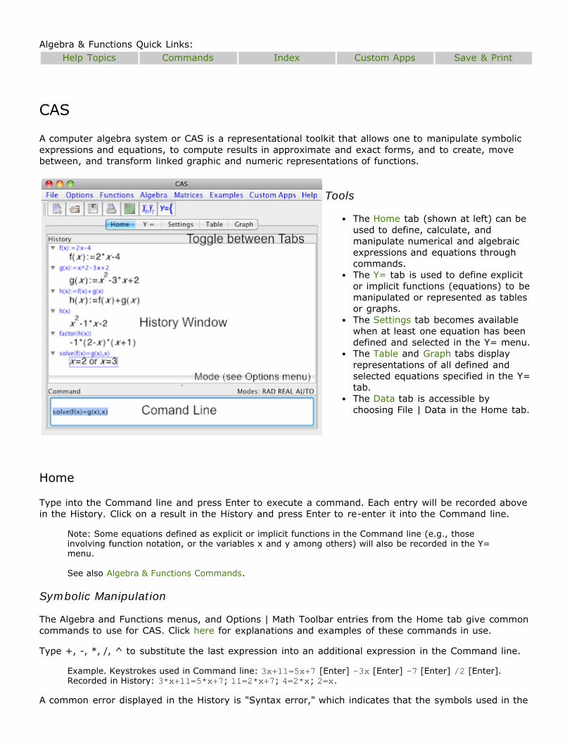
Tools

The Home tab (shown at left) can beused to define, calculate, andmanipulate numerical and algebraicexpressions and equations throughcommands.The Y= tab is used to define explicitor implicit functions (equations) to bemanipulated or represented as tablesor graphs.The Settings tab becomes availablewhen at least one equation has beendefined and selected in the Y= menu.The Table and Graph tabs displayrepresentations of all defined andselected equations specified in the Y=tab.The Data tab is accessible bychoosing File | Data in the Home tab.

Home

Type into the Command line and press Enter to execute a command. Each entry will be recorded abovein the History. Click on a result in the History and press Enter to re-enter it into the Command line.

Note: Some equations defined as explicit or implicit functions in the Command line (e.g., thoseinvolving function notation, or the variables x and y among others) will also be recorded in the Y=menu.

See also Algebra & Functions Commands.

Symbolic Manipulation

The Algebra and Functions menus, and Options | Math Toolbar entries from the Home tab give commoncommands to use for CAS. Click here for explanations and examples of these commands in use.

Type +, -, *, /, ^ to substitute the last expression into an additional expression in the Command line.

Example. Keystrokes used in Command line: 3x+11=5x+7 [Enter] -3x [Enter] -7 [Enter] /2 [Enter].Recorded in History: 3*x+11=5*x+7; 11=2*x+7; 4=2*x; 2=x.

A common error displayed in the History is "Syntax error," which indicates that the symbols used in the

previously entered command may be out of order, missing, or inappropriately used. Check for correctspelling and use of parentheses.

Settings

Setting the mode and default display of computations is done using the Home | Options menu.

See also Settings for Graphs and Tables.

The default Mode is Radian. Choose Options | Degree Mode to compute in degrees instead.

Note: The mode must be set in the Home tab; this setting applies to the entire CAS (Home,Y=, Settings, Table and Graphs).

Select Options | Complex Numbers to compute in this field (the default is Real numbers). Thisentry must be selected for i to be defined as the square root of negative one.Choose Options | Set # of Digits to determine the numerical display of computed expressions.Choose from 0, 1, 2, 3, 4, 5, 6 or All (the default is 4).By default, results are automatically simplified (Options | Auto Simplify).To show approximations of numeric computations, select Options | Auto Numeric.

For example, in Auto Numeric mode type 2/3 to yield .6667. Otherwise, 2/3 will be displayed.

Note: Another way to express numeric expressions in decimal form is to contaminate anexpression with a period ".". For example, compare the results of expressions (4./5)^2 (aperiod after the 4) and (4/5)^2 (no period).

Matrices

Use the Home tab Matrices menu to define new matrices, edit existing matrices, perform matrixcomputations, and view matrices as vertex-edge graphs.

There are several ways to define new matrices:

Choose Matrices | New Matrix and follow the prompts:1. Give the matrix a simple name (e.g., a single character "m" or short word(s) without

spaces).2. Type a numeric value for the number of rows, a comma, and a numeric value for the

number of columns (e.g., 2,3 for a 2x3 matrix).3. Type the values for each cell of the matrix then choose Matrix | Save to record the matrix

in the history.Type into the Command line with the following syntax:

matrixName:=[[column 1],[column 2],...[column n]]

where [column 1] is a list of the entries of the first column in the form [a11, a21, ...,an1] such that a11 is the first entry of the first column, a21 is the second entry of the firstcolumn, and so on.

Select an entry of the Examples menu or Sample Matrices. For instance:m:=matrix(2,3) Let the character m reference a 2x3 zero matrix. Type m Enter in the

Command line to call this matrix.m:=matrix(2,2,a,b,c,d) Let the character m reference a 2x2 matrix with row entries a, b, and c,

d. Type m Enter in the Command line to call this matrix.m:=[[1,2],[3,4]] Let the character m reference a 2x2 matrix that is defined by its first

and second columns: [1,2] and [3,4]. Note: Be sure to include acomma (",") between the two column matrices.

To edit a matrix:

Choose Matrices | Matrix Editor. Select a matrix to Edit. Type into the Matrix Editor window thenSave when finished.

Note: The Matrix Editor | Edit menu offers options to Add Row, Add Column Delete Row, andDelete Column. Click in the desired cell then choose an Edit menu option.

Click on a matrix in the Home | History to box it, press Enter. Edit the matrix values within theCommand line, press Enter when finished.

To compute with matrices type into the Command line or use the Matrix | Functions menu. Click belowto view an explanation of a command and see examples of its use:

matrix(), inv(), det(), id(), tr(), size(), row(), col().

View a matrix as a Directed or Undirected Vertex Edge Graph by choosing the desired entry fromHome | Matrices | View Matrix As. The selected matrix will be treated as an adjacency matrix and willbe represented as a vertex-edge graph in a new window.

See also Advanced Apps | Vertex-Edge Graphs.

Y=

The Y= tab is used to define, select, and edit equations and functions that can later be viewed in theTable or Graph tabs.

Define Equations and Functions

In general, any explicit or implicit equality or inequality that relates variables is an allowable functionthat may be defined in either the Y= tab or the Home tab. Some Help Tips are included below:

Parametric functions, piecewise functions, and three-dimensional curves can also be defined;examples of each are given in the Y= tab Examples menu.

See also Algebra and Functions Commands, Matrices.

To define f(x) as a function, f(x):= is the appropriate syntax.Use dependent variables that are distinct when you want to view a simultaneous table of values.For example, y1=x+2 and y2=-2x-3.In an explicit or implicit expression relating variables, the letter closest to z is treated as thedependent variable (i.e. plotted on the vertical axis, commonly the y-axis).A list of defined functions can be saved as a text file to use later.

See also Save & Print.

Select and Edit Equations and Functions

Type into the Y= Command line end press Enter; it will be listed below. Options to box and selectequations/functions include:

Box an equation by clicking on it to edit or delete it.

Press Enter to re-execute a boxed equation in the Command line to edit it (or chooseEdit | Edit Boxed Equation). Choose Edit | Delete Boxed equation to remove it from the Y= list.

Choose Edit | Clear All to erase all currently defined equations listed in the Y= tab.

Select an equation by clicking the check box to the left of it to view it's Settings, Graph, andTable.

If there is no check mark to its left, the equation is not selected and the settings, graph, andtable cannot be viewed.

Choose Edit | Select All or (Edit | Deselect All) to check (or uncheck) all listedequations/functions at once.

Settings and Plot Options

When an equation has been defined, a pull down options menu becomes available to its left. Use thismenu to select from Rectangular, Polar, Parametric, or 3D plot options.

See also Home | Settings, Settings tab.

Choose Rectangular for the standard Cartesian plane with horizontal and vertical axes representingthe independent and dependent variables, respectively.Choose Polar for a polar grid which plots the radial distance from the origin and the polar angle.When a parametric function has been defined (of the form XY=[x(t),y(t)]) the Parametric optionwill automatically be checked. Otherwise, this option will remain unchecked.Choose 3D to accept an implicitly defined or explicitly defined function in three or fewer variablesas defining a 3D curve. This option is useful when an equation such as x^2+y^2=2 is intended torepresent a cylinder (3D mode) instead of a circle (2D mode). If the 3D option is not selected,implicitly and explicitly defined functions will be interpreted as representing 2D curves or lines.

Settings

The Settings tab allows you to modify the window options and plot styles that pertain to the Graph taband Table tab. The Settings tab applies to all functions defined and selected in the Y= tab. Availableoptions depend upon whether a function is 2D (explicit or implicit) or 3D.

Note: A check mark must be next to at least one equation/function within the Y= tab for the Settingstab to be available.

See also Home tab Settings.

Options

Quickly modify settings for graphs and tables with the Options menu.

Choose Options | Standard Window ( ) to change the graph window to the standard view:domain=(-10, 10) and range=(-10, 10).Choose Options | Trig Window ( ) to change the graph window to the standard trigonometricview. In Degree mode: domain=(-360, 360) and range=(-3, 3). In Radian mode: domain=(-2pi,2pi) and range=(-3, 3).

Note: The Mode (Degree/Radian) should be set prior to executing trigonometric commands andadjusting settings.

See also Home tab Settings.

When Options | Simultaneous is checked settings will be grouped. Otherwise they will beseparated by tabs.

2D Functions

The 2D Functions tab within the Settings tab pertains to all selected functions that are defined explicitlyfrom within the Y= tab (e.g., the dependent variable is written as a function of the independent variablesuch as y=x+2).

Note: If Options | Simultaneous is not checked, then each explicitly defined function will have its ownsub tab to adjust settings individually.

Plot Style can be set to: Points Only (at Delta X step interval), Line/Curve, and Points withConnections.Minimum and Maximum X and Y: Type values and press Enter to set the lowest and highestbounds for the horizontal (independent, x-) and vertical (dependent, y-) axes on the Graph and

starting value for the Table.Set Delta X (or change in x, the independent variable) to determine the plot display and grid linesfor the Graph and interview for the Table.Select Auto Scale (Fit) to define the graph window to fit the selected function.

The Implicit sub tab within the Settings tab pertains to all selected functions that are defined implicitlyfrom within the Y= tab (e.g., 4x+y=8). Minimum and maximum x and y values can be set for this typeof 2D Function.

3D Plots

Settings for 3D Plots can be changed for each plot that is defined. Values for minimum and maximum X,Y, and Z coordinates can be changed for both the View Bounds and Graph Bounds.

View Bounds:Check Use Window Bounds so an appropriate viewing window is used automatically.Check Show Axes and Bounding Box to display these graph features.Check Show XYZ Orientation to show axes for clarity when rotating the plot.Change the View from 3D to XY, XZ, or YZ if you are interested in seeing the two-dimensional plane view.

Graph Bounds:If multiple 3D plots are checked, choose the one you want to set Graph Bounds on from theSelect Existing drop-down.Adjust the appearance of each 3D plot including the minimum and maximum graph boundsfor each axis.The "discr" setting determines how fine-grained the graphical view will be within theminimum and maximum values for X, Y, and Z.

Note: When simultaneously graphing multiple 3D functions it may be helpful to make one ofthe plots Transparent and to Color By: Z to better view the intersection.

Tables

The Table tab becomes available once an explicitly defined 2D Function or a 3D Plot is selected withinthe Y= tab. The settings that were determined within the Settings tab apply to the Table tab. SomeHelp Tips are include below:

See also Settings | Options.

If you are unable to view the contents of the Table tab, check the Y= tab. There must be a checkmark next to an explicitly defined 2D Function or a 3D Plot.You can view the table of values for more than one 2D function at a time. In this case, it is helpfulto define the functions using different function names.

For example, using y1(x):=8cos(x-30)+2 and y2(x):=6sin(x-60)+3 will give y1 and y2as headers in the table, helping to distinguish between the two.

When viewing the table for a 3D plot, it is best to view them one at a time. Also, selecting any ofthe index check boxes at the left will highlight the corresponding grid point in the 3D plot.To view more values than displayed in the table for a 2D function, click on a table entry then usethe up or down arrow key on the keyboard.

See also Save & Print.

Graphs

The Graph tab becomes available once a function is defined and selected within the Y= tab. The window

settings that are chosen from within the Settings tab determine the initial graphical display. Also usethe Zoom and View Options to customize the display.

Note: To trace (i.e., view the coordinates of points) a graph move the cursor over the graph.

See also Save & Print.

Zoom Settings

Determine the Window in the Settings tab or use the Graph tab Zoom menu:

Choose Zoom Box then drag a box around the desired section of the graph to zoom in on.Choose to Zoom In on the current plot to cut the window range in half.Choose to Zoom Out on the current plot to double the window range.Select Zoom Sqr to adjust the window range to be a square (relative to the window size).Choose Zoom Std to set the domain and range from -10 to 10, the Standard viewing window.Select Zoom Trig to set the domain to (-360,360) or (-2pi, 2pi) and the range to (-3,3),appropriate for trigonometric functions.

Note: Set the mode in the Home | Options menu before adjusting the window or zoomsettings.

Graph View Options

Options menu:

Select Options | Split View with Table to show the Table to the right of the graph. Otherwise thegraph is shown by itself.Choose to Show Equation, Draw Axes, and Draw Grid. When unchecked, the equation, axes, andgrid are hidden.

Note: Choose Options | Polar Grid to show (or hide) a polar grid. It may be useful to hide the(Cartesian) grid when this options is selected.

For a 3D plot, choose Options | Shading to add shading to the curve/surface.Choose the button to show (or hide) parameter Sliders. Each parameter will have its ownslider bar named according to how it was defined.

Note: This option pertains to plotted functions that include parameters. For example, defineand select y=a*x+b in the Y= tab. Notice the slider bars for a and b within the Graph tab.

Drag and release the slider to adjust the value of each parameter. Or, click on the name ofa slider then type its value to adjust it.When selected, Options | Sliders Snap to Mark allows parameter sliders to adjust at stepintervals. Otherwise, sliders are prevented from snapping to marks.

Slice 3D Plots

The Slice menu of the Graph tab is only available when viewing 3D Plots. It allows you to position aslicing plane, parallel to either the x-y plane, y-z plane, or x-z plane, and examine how the slicing planeintersects the 3D plot(s).

Check On in the Slice menu to enable a slicing plane in the 3D Plots display. Otherwise the slicingplane is hidden.Check Hide Surfaces in the Slice menu while On is checked to hide the 3D plot(s). This allows youto focus solely on the intersection of the slicing plane with the 3D plot(s) without those curvesobscuring anything.Choose a slicing option--Slice X ( , Y-Z Plane), Slice Y ( , X-Z Plane), or Slice Z ( , X-YPlane)--to enable the view of a slicing plane. Drag the slider to move the slicing plane across theviewable window.

Data

To view a data tab, choose File | Data in the Home or Y= tab.

Help topics on Data sheets are available in the Data Analysis Help. Note however that Data tabfunctionality is slightly different than the Data Analysis tool:

Scatterplot ( ) is the only Graph menu option available within the Data tab. Access the StatisticsData Analysis tool to use other graph options such as Histogram and Box Plot.

Note: If you choose to plot a scatterplot from data within the Data tab of CAS, the scatterplotwill be available within the Graph tab. Choose to plot functions over the scatterplot by selectingthem in the Y= tab. Also plot multiple scatterplots in the same window by enabling more thanone from within the Y= tab and adjusting the window Settings as needed.

Summary Statistics and Custom Apps for Statistics are not available within the CAS Data tab.Access the Statistics Data Analysis tool instead.

Algebra & Functions Quick Links:Help Topics Commands Index Custom Apps Save & Print

Spreadsheet

A spreadsheet allows one to display and compute data stored in the cells of a grid, and relate rows andcolumns by formulas.

Basics

Cells are referenced according totheir location by column (verticalarrangement is alphabetized byletter) then row (horizontalarrangement is numbered).

For example, the cellhighlighted at left is "C3"(column C, row 3).

Select a single cell by clicking on it.To select multiple cells at a time: (1)click and drag over a region with themouse, (2) hold down the Shift keywhile you click, or (3) hold down theControl key while you click to selectnon-adjacent cells.

Formulas

Formulas in a spreadsheet allow cells to be related so that the entry of one cell can be calculated from avalue or values in different cells.

See also Insert Function, Examples.

Getting Started

Some general tips on using formulas are listed below:

To enter a formula, type an equals sign (=) and then the formula you wish to use. Press Enter.Single-click a cell to view the formula used to compute it. Double-click a cell to edit the formula.Cells can be used in calculations by referencing their cell name. Any cell referenced in a formulamust contain a numerical value or the formula will produce an error. For example:

=B1^2+5 If cell B1 has a value of 2, the cell containing this formula will get the value of thesquare of cell B1 plus 5 (i.e., 2^2+5=9).

Place a dollar sign ($) in front of the column or row reference to fix the reference of thatparticular column or row. The row and/or column that is fixed will not change if that cell is copiedand pasted or filled down a particular column. For example:

=$B1^2+5 Fixes the column reference (column B) and allows the row reference (row 1, 2, 3,etc.) to vary.

=B$1^2+5 Fixes the row reference (row 1) and allows the column reference (column B, C, D,etc.) to vary.

=$B$1^2+5 Fixes both the column (column B) and row (row 1) references.

See also Examples.

Fill Down, Column Formula

Both the Fill Down and Column Formula entries of the Edit menu allow you to apply formulas to entireregions of cells at a time. This saves time in entering formulas.

Choose Edit | Fill Down or to apply a given formula to the selected cells below it.

See also Examples.

Select a column (click in a cell of the desired column), then choose Edit | Column Formula. In aseparate dialogue box, type the desired formula, then click OK (e.g., "=A1+2"). The enteredformula will then be applied to the entire column that was selected.

See also Getting Started.

Insert Function

Choose Insert | Function for a listing of common functions. Click on a function name below for a fulldescription of its use:

See also Algebra & Functions Commands.

Basic Statistics Trigonometric Combinatorics Other Functionssum()average()stdev()count()max()

sin()invsin()cos()invcos()tan()invtan()

perm()comb()fact()floor()ceil()

abs()sqrt()root()log()ln()exp()

If inserted into an empty cell, simply type between the parentheses (i.e., "=functionname()"). If theselected cell is not empty, the function name will be inserted at the end of those contents. To beexecuted as a formula, you must use the equals sign "=" immediately preceding the function name.

Examples

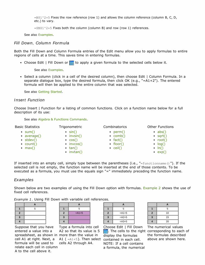
Shown below are two examples of using the Fill Down option with formulas. Example 2 shows the use offixed cell references.

Example 1. Using Fill Down with variable cell references. A1 5

2

3

4

A1 5

2 =A1+5

3

4

A1 5

2 =A1+5

3 =A2+5

4 =A3+5

A1 5

2 10

3 15

4 20

Suppose that you haveentered a value into aspreadsheet, as shown incell A1 at right. Next, aformula will be used torelate each cell in columnA to the cell above it.

Type a formula into cellA2 so that its value is 5more than the value inA1 ( =A1+5). Then selectcells A2 through A4.

Choose Edit | Fill Down . The cells to the right

display the formulascontained in each cell.NOTE: If a cell containsa formula, the numerical

The numerical valuescorresponding to each ofthe formulas describedabove are shown here.

value of the formula isshown unless theindividual cell is selected.

Example 2. Using Fill Down with fixed and variable cell references. A B1 5

2 10

3 15

4 20

A B1 5 =A$1^2+A1

2 10

3 15

4 20

A B1 5 =A$1^2+A1

2 10 =A$1^2+A2

3 15 =A$1^2+A3

4 20 =A$1^2+A4

A B1 5 30.0

2 10 35.0

3 15 40.0

4 20 45.0

Suppose you have dataentered in column A.Next, a formula will beused to relate each cellin column B to a fixedcell and a variable cell incolumn A.

Enter a formula into cellB1 so that its value isthe square of cell A1 plusthe correspondingcolumn A cell value. Thenselect cells B1 throughB4.

Choose Edit | Fill Down to obtain the desired

formulas in cells B2through B4, as shown tothe right. Notice thefixed and variablereferences used.

The numerical valuescorresponding to each ofthe formulas asdescribed above areshown here.

Edit and Insert Options

The Edit and Insert menus offer functionality to move and shift cells, delete and insert rows andcolumns, and to modify settings and styles of spreadsheet cells.

Move and Shift Cells

Use the Edit menu, toolbar icons, or keyboard shortcuts for quick cut, copy, and paste options forselected regions of cells. Also shift cells or regions of cells at a time.

See also Delete Column(s)/Row(s) and Insert Column(s)/Row(s).

From the Edit menu, choose to Cut or Copy (control+C) selected cells and temporarilystore them on the clipboard.

Note: The temporary storage will be replaced when anything else is cut or copied.

Choose Edit | Paste (control+V) to view the cut or copied cells on the clipboard. Be sure toclick on the the top-left cell of the rectangular region to be pasted into before pasting.Choose Insert | Shift Cells Right/Down to move the cell or selected region of cells accordingly.

Note: Any cells that were to the right of/below the selected cells also get shifted to theright/down to make room for the selected cells. Cell formulas are updated where necessary ascells move.

Delete and Insert Row(s)/Column(s)

Use these options to remove and shift entire row(s) and column(s) of a spreadsheet at a time:

Choose Edit | Delete Row(s)/Column(s) to remove the selected row(s)/columns(s) from yourspreadsheet. Any contents that were below/to the right of the deleted selection remain.

Note: This action cannot be reversed.

See also Cut, Copy, Paste.

Choose Insert | Row(s) to add a row above the selected cell. Choose Insert | Column(s) to add acolumn to the left of the selected cell.

See also Shift Cells right or down.

Settings and Styles

Customize the display of cells including the vertical alignment, the number of digits displayed (includingincrease and decrease by one), and the mode. Also choose to edit the column name from the defaultalphabetical name.

See also Sort data.

Choose Edit | Align to specify the horizontal position of text within a selected column. Thealignment options are Left ( ), Center ( ), and Right ( ).Choose Edit | Set # of digits to determine the number of decimals that are displayed for any dataentry that is in formula format (e.g., =0.14) in the selected column(s). You may choose to show0, 1, 2, 3, 4, 5, 6, or All decimal values (the default setting is 6). Alternatively, select the desiredcolumn(s) then choose (or ) to decrease (or increase) the number of digits (decimal places)by by one.

Note: When you manually type a number in a cell that is not a formula it is assumed that thedesired # of digits (decimal places) is already set. The Set Digits options only apply toformulas.

Choose Edit | Column Name then type the desired name into the "Edit Column Name" box. ClickOK to change the name from the default naming.

Note: If a column is renamed, you may use the new column name within a formula (as long asthe first characters in the name are not numerical) by typing the first characters of the nameuntil the first space. For example, suppose column A is renamed to "Test." In column B type=A1*3 OR =Test1*3.

Choose Edit | Degrees or Edit | Radians to set the mode of displayed computations in degrees orradians, respectively. The default setting is Degrees.

Tools

Most tools available in spreadsheet are also available within the Statistics | Data Analysis tool. Optionsto Sort, Graph, or view Summary Statistics are explained below.

Sort

The two Tool menu options for sorting data are Sort All Rows by and Sort All Columns by. Two differentmethods for using these features are suggested below:

1. Sort groups of rows/columns at a time.Without cells selected, choose a sorting option ( , )."In": Control+Click the desired rows/columns to group together and include in the sorting."By": Control+Click the desired rows/columns to determine the sorting (the selectedrow/column listed first will determine the primary sorting). Click OK.

Note: This method is desirable if the spreadsheet cells are related to one other (e.g., bivariatedata with pairings by rows).

2. Sort select rows/columns individually.Select the desired rows/columns to sort. Control+Click to select non-adjacent cellsChoose the desired sorting option ( , ). Only the selected cells will be sorted, all othercells will remain unsorted.

Note: This method is not desirable if the spreadsheet cells are related to one other (e.g.,bivariate data that include specific pairings).

Graph

Spreadsheet graph options are organized by type below. The links on each graph type redirect toadditional help topics within Data Analysis (or Advanced Apps for Contour plots):Univariate Bivariate Statistical Multivariate

HistogramBox Plot

ScatterplotMatrix Plot

Times SeriesNormal Plot

Contour / 3D Plot

Use a single column, orControl+Click to selectmore than one column ofdata for a "stacked"graph.

Two (or more) columnsmust be selected.Scatterplots require oneindependent and onedependent column.

May involve more thanone column of data(multi-column graphs willbe color-coded).

Uses the number of rowsand columns todetermine the size of thegrid and the entries ofthese cells as the"height" of the contourplot.

Summary Statistics

Choose Tools | Summary Statistics to compute Descriptive statistics (n, mean, minimum, q1, median,q3, maximum, sample standard deviation, and sample variance) and analyze Regression based on aselected model (linear, quadratic, cubic, quartic, power, exponential, logarithmic, polynomial, sinusoidal).

Note: For Regression analysis first choose the independent and dependent variables, then click OK. Aseparate Regression Analysis Frame will appear with Results, Graph, and Residuals in tabs across thetop.

See also Statistics & Probability for additional help topics.

Data

Choose a data set from the Data menu for quick access to pre-loaded data examples.

See also Data Sets for more information.

Algebra & Functions Quick Links:Help Topics CAS Spreadsheet Commands Index

Algebra & Functions Custom Apps

The Custom Apps for Algebra & Functions focus on graphical representations of functions. A descriptionand help topics for each of these tools is given below:

Function Iteration Linear Programming

Function Iteration

Illustrate the graphical iteration process for functions.

Instructions:

1. Determine the functionThere are multiple ways to determine the desired function to be used with this tool: (1) drag thea and b sliders (or click the buttons) to vary the parameters for the linear function f(x)=a*x+b;(2) type into the text box to the right of "f(x)=" to replace the given expression with one of yourchoosing; (3) select an entry from the Examples menu; (4) choose Now-Next from from theIteration menu for an alternative form for determining the function.

2. Set the initial valueType an Initial Value into the text box just above the table and press Enter. Equivalently, drag thered point along the x-axis to adjust the initial value dynamically.

3. Control the iteration speed and window viewThe Controls menu entries and their corresponding toolbar buttons allow you to start ( ), pause (

), reset ( ), and determine the speed ( ) at which the iterations are performed. Utilizefeatures of the Iteration menu, View menu, and Options menu to customize the way the graphicaliteration process is performed and is viewed.

4. View time series plotChoose the button to view a time series plot of the number of iterations versus the evaluatedfunction values. Click this button a second time to toggle back to the web view.

5. Save or print screenUse the entries of the File menu and its corresponding buttons to save ( ) or print ( ) thecurrent screen. Files are saved as images so the ".gif" filename extension is appropriate whensaving and naming files.

See also Save & Print.

Iteration menu

Choose Iteration | Show Fixed Points ( ) to highlight fixed points (if any) and display their valuebelow the graph. Select this option again to hide any fixed points.Select Iteration | Show Web ( ) to show (or hide) the web created through the iteration process.Select Iteration | Time Series ( ) to toggle between the graph of the function and a time series

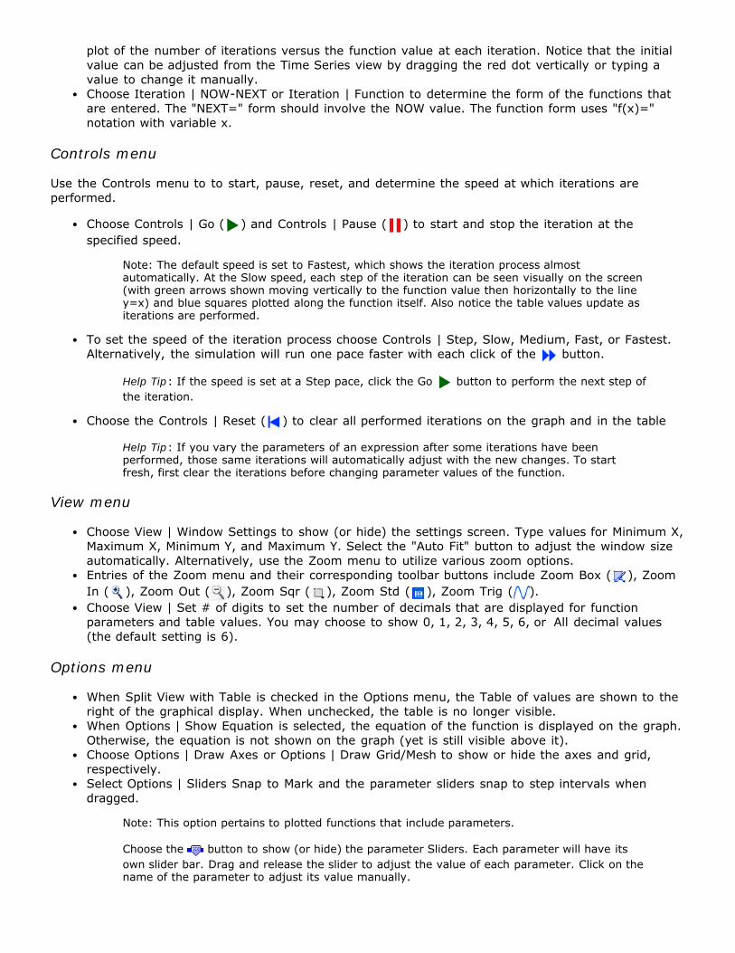
plot of the number of iterations versus the function value at each iteration. Notice that the initialvalue can be adjusted from the Time Series view by dragging the red dot vertically or typing avalue to change it manually.Choose Iteration | NOW-NEXT or Iteration | Function to determine the form of the functions thatare entered. The "NEXT=" form should involve the NOW value. The function form uses "f(x)="notation with variable x.

Controls menu

Use the Controls menu to to start, pause, reset, and determine the speed at which iterations areperformed.

Choose Controls | Go ( ) and Controls | Pause ( ) to start and stop the iteration at thespecified speed.

Note: The default speed is set to Fastest, which shows the iteration process almostautomatically. At the Slow speed, each step of the iteration can be seen visually on the screen(with green arrows shown moving vertically to the function value then horizontally to the liney=x) and blue squares plotted along the function itself. Also notice the table values update asiterations are performed.

To set the speed of the iteration process choose Controls | Step, Slow, Medium, Fast, or Fastest.Alternatively, the simulation will run one pace faster with each click of the button.

Help Tip: If the speed is set at a Step pace, click the Go button to perform the next step ofthe iteration.

Choose the Controls | Reset ( ) to clear all performed iterations on the graph and in the table

Help Tip: If you vary the parameters of an expression after some iterations have beenperformed, those same iterations will automatically adjust with the new changes. To startfresh, first clear the iterations before changing parameter values of the function.

View menu

Choose View | Window Settings to show (or hide) the settings screen. Type values for Minimum X,Maximum X, Minimum Y, and Maximum Y. Select the "Auto Fit" button to adjust the window sizeautomatically. Alternatively, use the Zoom menu to utilize various zoom options.Entries of the Zoom menu and their corresponding toolbar buttons include Zoom Box ( ), ZoomIn ( ), Zoom Out ( ), Zoom Sqr ( ), Zoom Std ( ), Zoom Trig ( ).Choose View | Set # of digits to set the number of decimals that are displayed for functionparameters and table values. You may choose to show 0, 1, 2, 3, 4, 5, 6, or All decimal values(the default setting is 6).

Options menu

When Split View with Table is checked in the Options menu, the Table of values are shown to theright of the graphical display. When unchecked, the table is no longer visible.When Options | Show Equation is selected, the equation of the function is displayed on the graph.Otherwise, the equation is not shown on the graph (yet is still visible above it).Choose Options | Draw Axes or Options | Draw Grid/Mesh to show or hide the axes and grid,respectively.Select Options | Sliders Snap to Mark and the parameter sliders snap to step intervals whendragged.

Note: This option pertains to plotted functions that include parameters.

Choose the button to show (or hide) the parameter Sliders. Each parameter will have itsown slider bar. Drag and release the slider to adjust the value of each parameter. Click on thename of the parameter to adjust its value manually.

Linear Programming

Analyze an optimization situation by using constraint inequalities and an objectivefunction to find the minimum/maximum. Both two-dimensional (2D) and three-dimensional (3D) linear programming problems can be examined.

The help topics below describe how to build a linear programming situation, how to analyze thatsituation, and how modifying the view can help bring forth features of the situation.

Build a Linear Programming Situation

Choose to Clear All the current drawing(s) and remove any constraint inequalities and objectivefunction that may be present. Alternatively, choose Tools | New to do the same.Enter a constraint inequality in the box next to the Constraint Inequalities checkbox. Use >= forgreater than or equal to and <= for less than or equal to. For a 2D problem, the default variablesused for function f are x and y; for a 3D problem, the defaults are x, y, and z. Repeat as neededuntil all constraint inequalities have been entered by first clicking the + button to add each newconstraint inequality.

Change the Variables: If desired, you can change the letters used to denote the functionand/or any of the variables. Be sure to first choose whether this will be a 2D or 3D problem bychecking or unchecking View | 3D. Select the Settings tab and rename the function/variables,making sure to hit Enter or Tab after you change an entry.

Enter the Objective Function as an expression (note that the left-hand side of the equation isalready provided).

Analyze the Situation

What is your purpose? Maybe you want to analyze the linear programming situation one constraintinequality at a time, resulting in the determination of the feasible region, and finalizing by using theobjective function to find the minimum/maximum. Or perhaps you want to skip all the details and getright to analyzing the feasible region. Your intent determines the way you use this tool.

View the region covered by a constraint inequality by clicking the checkbox next to that inequality.The window settings for the display automatically adjust to accommodate the new graph. Continueto click checkboxes to show all constraint inequalities graphed simultaneously (presumablyshowing a region of overlap, the feasible region).

Show Only Positive Values: Typically for a linear programming situation, you are onlyinterested in considering positive values. Thus, the default setting in the Constraints menu is todo just that, Show Only Positive Values.

View only the boundary values of the region covered by a constraint inequality by selectingConstraints | Show Only Boundary.View the feasible region by selecting Constraints | Show Feasible Region or by clicking the button.Choose the or buttons to change the axis of rotation to the y- or z-axis, respectively.

Tool menu

The Tool menu offers options to Restart, Print, and Close the custom app.

Choose Tools | Restart to give the original starting view, settings, and graph.Choose Tools | Print to print the currently selected frame.

See also Save & Print.

Options menu

The Options menu allows you to modify the display of the 3D surface of revolution.

Choose Options | Show Edges to toggle the wireframe of the surface of revolution.Choose Options | Show Surface to toggle the quadrilateral faces that comprise the surface ofrevolution.Choose Options | Show Meridian to toggle the 2D curve used to sweep out the surface ofrevolution.Select Options | Show 3D Axes to toggle the x-y-z coordinate axes.Choose Options | Rotate about Horizontal Axis ( ) to perform the revolution about the y-axisrather than the z-axis. Alternatively, choose Options | Rotate about Vertical Axis ( ) to performthe revolution about the z-axis rather than the y-axis.

Algebra & Functions Quick Links:Help Topics CAS Spreadsheet Commands Catalog

Algebra & Functions Index

All help topics and commands that are available within the Algebra & Functions tools are listed below inalphabetical order.

2D Functions3D Plots, Bounds3D Plot Option (CAS)3D Plot (Spreadsheet) abs() ans(1) Adjacency MatrixAdvanced Apps Algebra & Functions CommandsAlignment ApproximateAuto NumericAuto ScaleAuto Simplifyaverage()Basic Statistics Functionsbinomcdf()binompdf() Box Plot CASceil() CellCell ReferenceCenter Alignchisqcdf()chisqpdf() Clear All (Y=) col()Column FormulaColumn Name comb() Combinatorics Functions CommandsCommand linecomplex() Complex Numbersconj() Contour Copy cos() count()Custom AppsCut Data (CAS)Data (Spreadsheet)

Data Sets Define EquationDegree Mode (CAS)Degree Mode (Spreadsheet)Delete EquationDelete Row, Delete ColumnsDelta Xder() Deselect Alldet()Directed Vertex Edge GraphDraw AxesDraw GridEdit Cells Edit EquationEdit FormulaExamples exp()expand() fact()Fcdf()Fpdf()Fixed Cell ReferenceFill Downfloor()FormulasFunction IterationGraph (CAS)Graph (Spreadsheet) Hide SurfacesHistogram Home tabi id()imag()ImplicitInsert CellsInsert Functionint() inv()invcos()invNorm()invsin()invT() invtan()

Left AlignLinear Programming ln() log() Math ToolbarMatricesmatrix()Matrix EditorMatrix FunctionsMatrix ExampleMatrix Plot max()Maximum Maximum X, YMeanMedian Minimum Minimum X, YMode (CAS)Mode (Spreadsheet)Move and Shift CellsN New MatrixNormal Plotnormalcdf()normalpdf() Options menu (Graph) Options menu (Home)Options menu (Settings)Other Functions Parameter Parametric Plot OptionPaste perm() piecewise() Plot Style Polar Plot Option Printprod() Q1Q3Radian Mode (CAS)Radian Mode (Spreadsheet)real()regeq()

Rectangular Plot OptionRegression Right Alignroot() row()Sample MatrixSample Standard DeviationSample Variance SaveScatterplot (CAS)Scatterplot (Spreadsheet)Select Equation Set # of Digits (CAS)Set # of Digits (Spreadsheet) SettingsSettings (Home)Settings (Y=) ShadingShift Cells Show Equation

simplify() Simultaneoussin()size()Slice 3D Plot Slice X, Y, Z Sliders, Snap to Marksolve() Sort Split View with TableSpreadsheet Standard Windowsqr() sqrt() stdev()sum() Summary Statistics (CAS)Summary Statistics (Spreadsheet)Symbolic ManipulationSyntax Error

Tabletan()tcdf()Time Series tr()tpdf() Trig WindowTrigonometric FunctionsUndirected Vertex Edge GraphView Matrix AsView Options (Graph)Y=Zoom BoxZoom InZoom OutZoom SettingsZoom SqrZoom StdZoom Trig

Algebra & Functions Quick Links:Help Topics CAS Spreadsheet Index Catalog

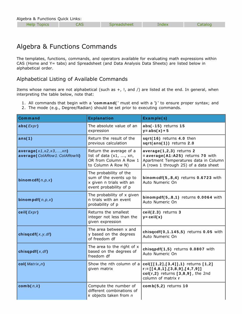
Algebra & Functions Commands

The templates, functions, commands, and operators available for evaluating math expressions withinCAS (Home and Y= tabs) and Spreadsheet (and Data Analysis Data Sheets) are listed below inalphabetical order.

Alphabetical Listing of Available Commands

Items whose names are not alphabetical (such as +, !, and /) are listed at the end. In general, wheninterpreting the table below, note that:

1. All commands that begin with a 'command(' must end with a ')' to ensure proper syntax; and2. The mode (e.g., Degree/Radian) should be set prior to executing commands.

Command Explanation Example(s)

abs(Expr) The absolute value of anexpression

abs(-15) returns 15y=abs(x)+5

ans(1) Return the result of theprevious calculation

sqrt(16) returns 4.0 thensqrt(ans(1)) returns 2.0

average(x1,x2,x3,...,xn)average(ColARow1:ColARowN)

Return the average of alist of data (x1, ..., xn,OR from Column A Row 1to Column A Row N)

average(1,2,3) returns 2=average(A1:A25) returns 70 withApartment Temperatures data in ColumnA (rows 1 through 25) of a data sheet

binomcdf(n,p,x)

The probability of thesum of the events up tox given n trials with anevent probability of p

binomcdf(5,.8,4) returns 0.6723 withAuto Numeric On

binompdf(n,p,x)The probability of x givenn trials with an eventprobability of p

binompdf(5,.8,1) returns 0.0064 withAuto Numeric On

ceil(Expr) Returns the smallestinteger not less than thegiven expression

ceil(2.3) returns 3y=ceil(x)

chisqcdf(x,y,df)The area between x andy based on the degreesof freedom df

chisqcdf(0,1.145,5) returns 0.05 withAuto Numeric On

chisqpdf(x,df)The area to the right of xbased on the degrees offreedom df

chisqpdf(1,5) returns 0.0807 withAuto Numeric On

col(Matrix,n) Show the nth column of agiven matrix

col([[1,2],[3,4]],1) returns [1,2]r:=[[4,8,1],[3,8,9],[4,7,9]]col(r,2) returns [3,8,9], the 2ndcolumn of matrix r

comb(n,k) Compute the number ofdifferent combinations ofk objects taken from n

comb(5,2) returns 10

objects

complex(a,b) When in ComplexNumbers mode, take anordered pair of realnumbers, (a, b), andreturn a complexnumber, a + bi

complex(-5,7) returns -5+7i

conj(Expr) Compute the complexconjugate of the givenexpression

conj(4+i) returns 4-i

cos(Expr) Evaluate the cosine ofthe given expression

cos(pi) returns -1 in Radian modey=cos(x/2)

count(x1,x2,...,xn)count(ColARow1:ColBRowN)

Gives the number ofelements in a list of data

count(1,2,3,4,5) returns 5=count(B1:C22) returns 44 within100-meter Freestyle data sheet

der(Expr,Var) Evaluate the derivative ofan expression withrespect a variable

der(x^2,x) returns 2xy:=der(x^3+x^2+x,x) returnsy:=3x^2+2x+1

det(Matrix) Calculate the determinantof a given matrix

det([[2,0],[4,2]]) returns 4t:=[[7,3],[2,1]]det(t) returns 1

exp(Expr) Gives the special number'e' and can be used as abase in expressions forexponential functions

ln(exp(x)) returns xsolve(exp(x)=20,x) returns x=ln(20)

expand(Expr) Rewrites an expression inan equivalent form thatdoes not containparentheses

expand((6-(45/3))^2) returns 81expand((6*x^2)*(4*x+12)) returns24*x^3+72*x^2

fact(n) Compute the factorial ofa natural number

fact(5) returns 120; equivalent to5*4*3*2*1

factor(Expr) Rewrites an expression infactored form, whenpossible

factor(3*x^2+6*x-24) returns3*(x+-2)*(x+4)

Fcdf(x,y,dfNum,dfDenom)

The area between x andy given the degrees offreedom of the numeratorand denominator

Fcdf(0,2.1,25,20) returns 0.9528 withAuto Numeric On

Fpdf(x,dfNum,dfDenom)

The area to the right of xgiven the degrees offreedom of the numeratorand denominator

Fpdf(5,25,20) returns 0.0004 withAuto Numeric On

floor(Expr) Returns the largestinteger less than or equalto the given expression

floor(6.7) returns 6y=floor(x)

i Defined as sqrt(-1) withComplex Numbers on

sqrt(-1) returns i

id(n) Show the nxn identitymatrix in matrix form

id(3) returns [[1,0,0],[0,1,0],[0,0,1]]in matrix form

imag(Expr) Returns the imaginary imag(6i+42) returns 6i

part of a complex number

int(Expr,Var,lowBound,upBound) Compute the definiteintegral of an expressionfrom lower to upperbound values

int(sin(x),x,pi,2*pi) returns 1-cos(2*pi) and -2 in auto simplify mode

inv(Matrix) Calculate the inverse of amatrix

inv([[2,2],[1,2]]) returns [[1,-1],[-1/2,1]]n:=[[1,1],[1,0]]inv(n) returns [[0,1],[1,-1]] in matrixform

invcos(Expr) The inverse cosine of anexpression

invcos(1.) returns 0y=invcos(x+pi)

invNorm(percentile,xbar,s)

The value given thepercentile rank withmean x-bar and standarddeviation s

invNorm(0.05,25,6) returns 15.1309with Auto Numeric On

invsin(Expr) The inverse sine of anexpression

invsin(1.) returns 90y=invsin(2*x-pi)

invT(pvalue,df)The t-value given a p-value and degrees offreedom df

invT(.05,61) returns 1.9996 with AutoNumeric On

invtan(Expr) The inverse tangent of anexpression

invtan(1) returns 45 in Degree modey=invtan((x/2)*pi)

ln(Expr) Take the natural log(base e) of an expression

ln(exp(2)) returns 2y=ln(x)

log(Expr) Take the log (base 10) ofan expression

log(100) returns 2y=log(6*x)

matrix(r,c,Expr,Expr,...Expr) Define a matrix with rrows, c columns, and itsentries by row

matrix(2,3,1,2,3,4,5,6) is a 2x3matrix with row entries 1,2,3 and 4,5,6m:=matrix(2,2,1,0,0,1) then mreturns the 2x2 identity matrix

[[col 1],[col 2], ..., [col k]] Define a matrix by itscolumn entries separatedby commas

[[2,3,0],[1,2,1]] returns a 3x2 matrixwith column entries 2,3,0 and 1,2,1k:=[[4,5],[7,9]] then k returns a 2x2matrix with row entries 4,7 and 5,9

max(x1,x2,...,xn)max(ColARow1:ColBRowN)

Determine the greatestvalue in a list of data

max(7,3,5,2,1) returns 7=max(B1:C22) returns 82.2 within100-meter Freestyle data sheet

normalcdf(x,y,xbar,s)The area between x andy with mean x-bar andstandard deviation s

normalcdf(-infinity,19.2,25,6)returns 0.1669 with Auto Numeric On

normalpdf(x,xbar,s)The area to the right of xwith mean x-bar andstandard deviation s

normalpdf(5,25,6) returns 0.0003with Auto Numeric On

perm(n,k) Compute the number ofdifferent permutations ofk objects taken from nobjects

perm(5,2) returns 20

piecewise(Expr,Expr,...) Create a piecewisefunction

y=piecewise(cos(x),x<0,1.5^x,0<=xAND x<=4) returns the two-part

piecewise function on the specifieddomain

prod(Expr,Expr,...,Expr) Multiply a list ofnumerical values

prod(5,4,3,2) returns 120prod(2*x,x^2,x^3) returns 2.0*x^6

prod(Expr,Var,Start,End) Find the product of avariable expression forthe specified variable fora range of numericalvalues from Start to End

prod(3*x,x,1,4) returns 1944 whichequals (3*1)*(3*2)*(3*3)*(3*4)

real(Expr) Returns the real part of acomplex number

real(-3i+10) returns 10

regeq(1) As long as a regression ofsome sort has alreadybeen performed onbivariate data, this willreturn the regressionequation itself

regeq(1) returns y=<the regressionequation>y=regeq(x) creates an equation in theY= tab, but does not display the specificequation

root(Expr,n) Take the nth root of anexpression

root(27,3) returns 3.0y=root(x,4)

row(Matrix,n) Show the nth row of agiven matrix

row([[3,0],[0,5],[7,0]],1); returnsfirst entries of each column, namely therow [3,0,7]w:=[[2,2],[3,4],[5,1]] then row(w,2) returns [2,4,1]

simplify(Expr) Rewrites an expression inan equivalent, simplifiedform

simplify(6+10) returns 16simplify((5x+3)*(2x+3)) returns10*x^2+21*x+9

sin(Expr) The sine of an expression sin(3*pi/2) returns -1.0 in Radianmodey=sin(x+3)

size(Matrix) Calculate the (row ,column) size of a matrix

size([[1,3,5],[7,9,11]]) returns [3 2]n:=[[2,2],[4,4],[6,6]] then size(n) returns [2 3]

solve(Equation,Var) Solve an equation orinequality for thespecified variable

solve(30=5*x^2+2*x+6,x) returnsx=-12/5 or x=2

sqr(Expr) The square of anexpression

sqr(17) returns 289y=sqr(11*x)

sqrt(Expr) The square root of anexpression

sqrt(225) returns 15y=sqrt(36*x^2+1)

stdev(x1,x2,...,xn)stdev(ColARow1:ColBRowN)

Computes the standarddeviation of a list of data

stdev(1,2,3) returns 1 =stdev(A1:A25) returns 2.16 withinApartment Temperatures data sheet

sum(Expr,Expr,...,Expr) Sum a list of numericalvalues or expressions

sum(5,6,7,8) returns 26.0sum(x,2x,-4x,17x,8x) returns24*x+0.0

sum(Expr,Var,Start,End) Find the sum of avariable expression withrespect to the variablefor a range of numerical

sum(x-4,x,1,4) returns -6

values from Start to End

tan(Expr) Evaluate the tangent ofan expression

tan(45) returns 1 in Degree modey=tan(pi/x)

tcdf(t1,t2,df)The area between t1 andt2 based on the degreesof freedom df

tcdf(-2,2,61) returns 0.95 with AutoNumeric On

tpdf(t,df)The area to the right of tbased on the degrees offreedom df

tpdf(1,61) returns 0.24 with AutoNumeric On

tr(Matrix) Transpose a given matrix tr([[1,2],[3,4]]) returns [[1,3],[2,4]]in matrix formP:=[[1,1,1],[2,2,2],[3,3,3]]then tr(P) returns[[1,2,3],[1,2,3],[1,2,3]] in matrixform

Expr+Expr Add; Returns the sum oftwo expressions

147+56 returns 203y=5*x+3

Expr at Var=ValueExpr @ Var=Value

At; Evaluate theexpression at theindicated value of thevariable

y=-x+3 at x=2 returns y=1y=-x+3 @ x=2 returns y=1

Expr/Expr Divide; Returns thequotient of twoexpressions

-135/27.0 returns -5.0y=1/x

Expr=Expr Equal to 23^2=529 returns true evaluationy=x

Expr>Expr Greater than 16*24/3>129 returns false evaluationy>2*x

Expr>=Expr Greater than or equal to 47*13>=649 returns false evaluationy>=6*x+4

Expr<Expr Less than 23*13<300 returns true evaluationy<10*x+2

Expr<=Expr Less than or equal to 65*7<=490 returns true evaluationy<=2*x-5

Expr%Expr Modulo 27%12 returns 3

Expr*Expr Multiply, take the productof

167*14 returns 2338y=6*x

Expr!=Expr Not equal to 9/167!=0.1 returns true evaluationy!=10+x

Expr^Expr Raise to the power of 36^4 returns 1679616y=2^(x+1)

Expr-Expr Subtract; negative value 64-13 returns 51y=3x^2-2x-1

Math Toolbar

Choose Math Toolbar in the CAS Home tab Options menu to view the Typing Palette. From the typingpalette, click on an available button to utilize it's functionality in the Command line.

Icon Command Icon Command

Expr/Expr <

^2 <=

sqrt() >=

root(Expr,n) >

sum(Expr,Var,Start,End) !=

prod(Expr,Var,Start,End)

Geometry & Trigonometry

Geometry and Trigonometry tools include an interactive drawing tool for constructing,measuring, manipulating, and transforming geometric figures, a simple object-oriented programming language for creating animation effects, and a set of customapps for studying geometric models in 2D and 3D. Interactive Geometry can belaunched in a synthetic or coordinate environment.

Synthetic Drawing

Measure & Calculate Custom Apps

Explore the possibilities ofdynamic geometry within asynthetic (non-coordinate)

environment.

Click and drag to createand move objects with

dynamic capabilities, selectshapes to modify their

properties.

Select an object and anattribute to be measured

and use measurements in aCalculation.

Experiment with pre-designed sketches,

animations, and dynamicfigures, with support from

on-screen prompts.Coordinate Constructions

Transformations

Program & Animate

Explore the possibilities ofdynamic geometry within acoordinate environment.

Select an object(s) and aconstruction option fordynamic designs thatalways remain true.

Flip, turn, slide, and scale adrawn geometric object to

a new location in theplane.

Execute a sequence ofcommands to define, draw,construct, and transform

objects in the plane.Index Commands Settings Save & Print

Browse help topics specificto Geometry &

Trigonometry in A-Z order.

Listing of availablecommands with examplesfor Interactive Geometry.

Modify stylistic attributesof created objects.

Core Math Tools (CMT),Image (GIF) and Text(TXT) are file types.

See also Help Topics at a Glance or Go Online for Additional Resources.

Geometry & Trigonometry Quick Links:Help Topics Commands Index Custom Apps Save & Print

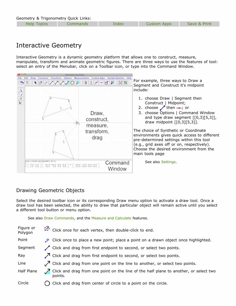
Interactive Geometry

Interactive Geometry is a dynamic geometry platform that allows one to construct, measure,manipulate, transform and animate geometric figures. There are three ways to use the features of tool:select an entry of the Menubar, click on a Toolbar icon, or type into the Command Window.

For example, three ways to Draw aSegment and Construct it's midpointinclude:

1. choose Draw | Segment thenConstruct | Midpoint;

2. choose then ; or3. choose Options | Command Window

and type draw segment [[0,3][5,3]],draw midpoint [[0,3][5,3]].

The choice of Synthetic or Coordinateenvironments gives quick access to differentpre-determined settings within this tool(e.g., grid axes off or on, respectively).Choose the desired environment from themain tools page

See also Settings.

Drawing Geometric Objects

Select the desired toolbar icon or its corresponding Draw menu option to activate a draw tool. Once adraw tool has been selected, the ability to draw that particular object will remain active until you selecta different tool button or menu option.

See also Draw Commands, and the Measure and Calculate features.

Figure orPolygon Click once for each vertex, then double-click to end.

Point Click once to place a new point; place a point on a drawn object once highlighted.

Segment Click and drag from first endpoint to second, or select two points.

Ray Click and drag from first endpoint to second, or select two points.

Line Click and drag from one point on the line to another, or select two points.

Half Plane Click and drag from one point on the line of the half plane to another, or select twopoints.

Circle Click and drag from center of circle to a point on the circle.

Angle Click three times to define a point, vertex, and another point; angle is determinedcounterclockwise from initial to final.

Vector Click and drag from initial point to second point, or select two points.

Selecting Objects

There are two common ways to Select drawn objects: use the tool (Shift click to select multiple), orchoose Help | List of Shapes (Control click to select multiple, close the window).

Once selected, objects can be moved by dragging. The style of selected objects can also be changed.

See also Transformations, Settings.

Measure and Calculate

To measure a drawn object, first select an object, then choose an attribute to be measured orcalculated from the Measurements menu. Double-click a measurement to modify the Calculation, Label,and see the result within a Calculation window.

Each measurement option and the objects that can be measured using that command are listed below:

Coordinates: Gives the matrix representation of any object drawn in the plane (defined by itspoints). Available within the Coordinate geometry environment only.

Note: All coordinate measurements will be represented by a matrix of size 2 x ? with the firstand second rows for the x- and y-coordinates, respectively. Each column represents thecoordinates of a single point. The Style of an object(s) can be changed to show coordinates asordered pairs.

Lengths: Gives the absolute value of the distance between points defining a segment, ray, line,half plane, circle, or angle.Angles: Gives the angle measure (in degrees) of an angle or all the angles in a figure or polygon.Slopes: Gives the slope of the segment, ray, line, half plane, or the segments defining a figure orpolygon, or angle.Perimeter/Circumference: Gives the total distance around a figure or polygon, collection ofsegments, or circle.Area: Gives the total space enclosed by a figure or polygon, or circle.

Choose Measurements | Calculation to perform a calculation using numerical values, or previously-calculated results or measurements. Within a Calculation window:

1. Type the desired calculation (e.g., +, -, /, *); click on the drop-down list to insert an existingmeasurement or result.

2. Choose a label for the calculation (or leave it blank) and click the Test button (this is what willdisplay on the screen).

3. Click OK to insert this labeled calculation into your drawing.

Constructions

Select an object(s) and a construction option from the toolbar or the Construct menu. Constructionsremain true regardless of how the original object(s) are dragged.

See also Construction Commands to program constructions within the Command Window.

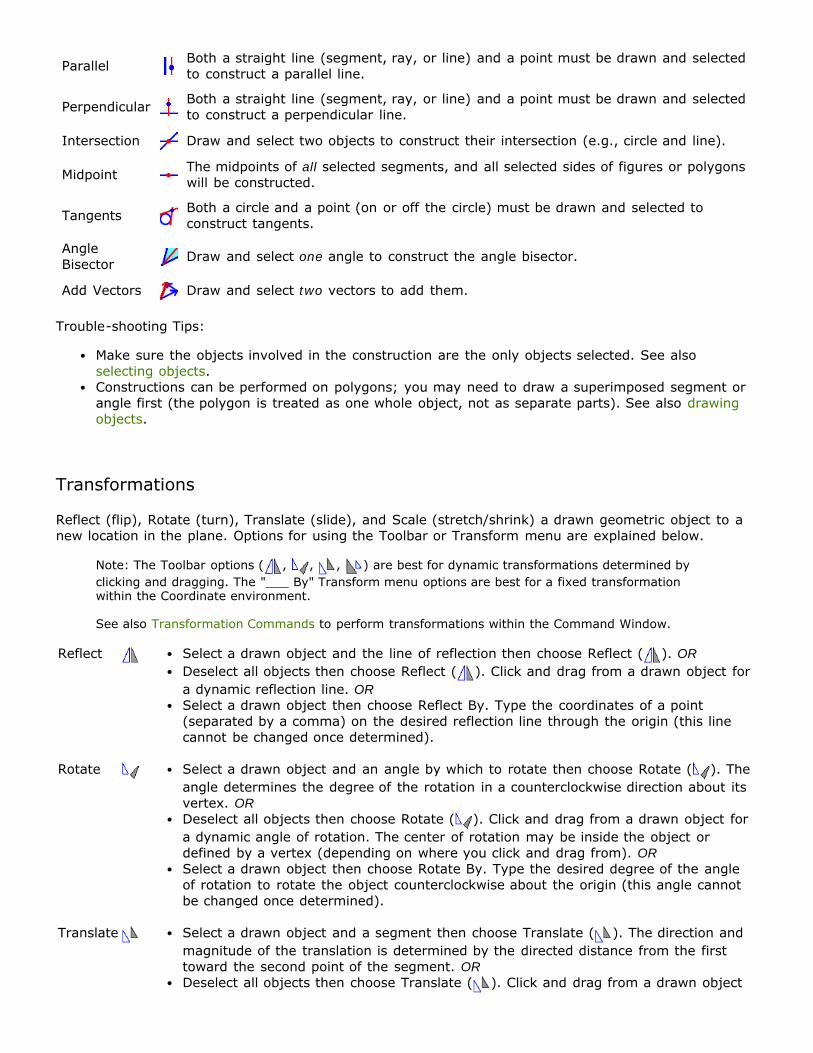
Parallel Both a straight line (segment, ray, or line) and a point must be drawn and selectedto construct a parallel line.

Perpendicular Both a straight line (segment, ray, or line) and a point must be drawn and selectedto construct a perpendicular line.

Intersection Draw and select two objects to construct their intersection (e.g., circle and line).

Midpoint The midpoints of all selected segments, and all selected sides of figures or polygonswill be constructed.

Tangents Both a circle and a point (on or off the circle) must be drawn and selected toconstruct tangents.

AngleBisector Draw and select one angle to construct the angle bisector.

Add Vectors Draw and select two vectors to add them.

Trouble-shooting Tips:

Make sure the objects involved in the construction are the only objects selected. See alsoselecting objects.Constructions can be performed on polygons; you may need to draw a superimposed segment orangle first (the polygon is treated as one whole object, not as separate parts). See also drawingobjects.

Transformations

Reflect (flip), Rotate (turn), Translate (slide), and Scale (stretch/shrink) a drawn geometric object to anew location in the plane. Options for using the Toolbar or Transform menu are explained below.

Note: The Toolbar options ( , , , ) are best for dynamic transformations determined byclicking and dragging. The "___ By" Transform menu options are best for a fixed transformationwithin the Coordinate environment.

See also Transformation Commands to perform transformations within the Command Window.

Reflect Select a drawn object and the line of reflection then choose Reflect ( ). ORDeselect all objects then choose Reflect ( ). Click and drag from a drawn object fora dynamic reflection line. ORSelect a drawn object then choose Reflect By. Type the coordinates of a point(separated by a comma) on the desired reflection line through the origin (this linecannot be changed once determined).

Rotate Select a drawn object and an angle by which to rotate then choose Rotate ( ). Theangle determines the degree of the rotation in a counterclockwise direction about itsvertex. ORDeselect all objects then choose Rotate ( ). Click and drag from a drawn object fora dynamic angle of rotation. The center of rotation may be inside the object ordefined by a vertex (depending on where you click and drag from). ORSelect a drawn object then choose Rotate By. Type the desired degree of the angleof rotation to rotate the object counterclockwise about the origin (this angle cannotbe changed once determined).

Translate Select a drawn object and a segment then choose Translate ( ). The direction andmagnitude of the translation is determined by the directed distance from the firsttoward the second point of the segment. ORDeselect all objects then choose Translate ( ). Click and drag from a drawn object

for a dynamic translation vector. ORSelect a drawn object then choose Translate By. Type the desired x- and y-components of the translation (this is fixed and cannot be changed oncedetermined).

Scale Select a drawn object and a segment then choose Scale ( ). The direction andmagnitude of the scale transformation is determined by the directed distance fromthe first toward the second point of the segment. ORDeselect all objects then choose Scale ( ). Click and drag from a drawn object for adynamic scale transformation determined by a directed segment. ORSelect a drawn object then choose Scale By. Type the desired x- and y- componentsof the scale vector (this is fixed and cannot be changed once determined).

Settings

Use the Options and Edit menus to control the Settings. In general:

use the Options menu to change the geometry environment settings for all created objects at onceor before objects are created (e.g., choose Options | Default Settings, and the settings will applyto all subsequently created objects);use the Edit menu to modify stylistic aspects of selected objects after objects are created (e.g.,select Edit | Change Style of Selected and the settings will apply to all currently selected objects).

A Style Window will appear after either of these options is selected (see illustration below).

See also Default Styles and Settings, Labels, Hide/Show or Delete Objects, and Undo.

Access the Style Window to adjust the following settings (Options | Default Settings OR Edit | Change Style of Selected):

Label objects (default on) by capital alphabetical labels inthe order they are created. See also Options | Hide Labels(hides all at once), and Edit | Label Change (replace defaultlabel)Show Coordinates (default off) labels points in Coordinategeometry with ordered pairs. See also Options | HideCoordinates.Filled objects (default off) will have their interior shadedaccording to the "Select Fill Color" palette (default gray).Visible (default on) is only accessible within the DefaultStyle window (Options | Default Settings).The Font Size (default 12) of labeled objects can beincreased or decreased.Thickness (default thin) of edges can be made thicker andEdge Color (default black) can be changed by using the“Select Color” palette.

Default Styles and Settings

The main difference between Synthetic and Coordinate Geometry environments is the Grid Style (seeOptions | Grid Style). The Grid and Axes are off (not shown) for Synthetic and on (visible) forCoordinate. In a Coordinate Geometry Environment the following settings are applicable:

Options | Snap to Grid (default on) restricts the drawing of points to grid marks. When notchecked plot points with non-integer coordinates.Options | Hide Coordinates (default off) will hide (or show) all coordinates at once. Use

Edit | Change Style of Selected to be more selective about which coordinates to show/hide.Options | Grid Style (default on) allows one to modify the grid points, thickness, style, and colorof grid marks.

Help Tip: Coordinate Labels are ordered pairs attached to points plotted in the coordinate planeand are a stylistic aspect of the geometry environment. To compute with matrixrepresentations of ordered pairs select the desired object(s) chooseMeasurements | Coordinates.

Options | Window Scale (default 20: [-10, 10]) takes a positive numerical value to set the viewingrange of the screen for both x- and y-axes (the screen will always be symmetrical about theorigin).Labels of drawn objects are shown by default. For a selected object, choose Options | Hide Labelsor Edit | Label Change. For Label Change, the current name is in the left-hand column, the newname is typed into the right-hand column. Close the window to change the label.

See also Style Window (Edit | Change Style of Selected OR Options | DefaultSettings).

Hide/Show or Delete a selected object using the appropriate Edit menu option (Edit | HideSelected, Show Hidden, Delete Selected).

Note: Show Hidden will make all previously hidden objects visible. Delete Selected ispermanent and cannot be reversed.

Edit | Undo ( ) reverses the most recently performed action(s).

Note: Deleted objects cannot be shown again. To temporarily hide/show objects use Edit | HideSelected.

Programming and Animation

Execute a sequence of commands to draw, construct, transform, and otherwise manipulate objects inthe plane.

Note: Although the Options | Command Window is accessible through the Synthetic environment,commands typically reference the coordinates of an object. It is therefore suggested that theCoordinate environment be used for programming.

See also Available Commands for Geometry.

Getting Started

There are several avenues to pursue programming within Interactive Geometry. Some are listed below:

Use the Design by Robot Custom App to test the use of simple commands to move the robotaround the screen (e.g., fd 10 rt 90 to move forward 10 units and turn 90 degrees).Create a drawing or construction within Interactive Geometry. Choose File | Save and use the .txtextension. Open this saved file within a Text Editor program on your computer. Read through theprogramming commands that were used to create the drawing you made. Also open a saved textfile within Interactive Geometry.Type into the Command Window (press Enter to execute a command).

To view the command window Choose Options | Command Window, or move your cursor tothe bottom of the screen and drag up from the small circle.

Type the program command (followed by a space and the name of your program) into theCommand Window to work within the Program Editor. Close this window then call the program bytyping its name. This is especially useful for longer programs or animations. For example:

program animateMe(type program into programming window, then close window)

animateMe

See also programming Basics.

Basics

See the Available Commands for Geometry.Do not use reserved words such as point or circle to name objects or programs. For example, agood command would be let pointA=point [0,0] (the name of the point is "pointA"). Otherreserved words include but are not limited to:

draw, polygon, point, segment, ray, line, halfplane, circle, angle,parallel, perpendicular, intersection, midpoint, clear, let, cs, info,show, reflect, rotate, translate, scale, visible

A space " " should follow all reserved word commands.Square brackets are used to enclose commands and ordered pairs (e.g., let segmentAB=segment[[0,0][5,3]], let M=[midpoint segmentAB]).let and draw (or visible) are basic commands to define and show objects.Clear the screen (cs) or the screen and command window contents (clear).The information or coordinates of an object can be shown on the screen (info) or within thecommand window (show).Commands for defining and drawing common objects include: angle, circle, halfplane, line,point, polygon, ray, segment, vector.

See also Drawing using the menubar/toolbar.

Construction commands include: bisect, intersection, midpoint, parallel, perpendicular,tangents.

See also and Constructions using the menubar/toolbar.

Transformation commands include: reflect, rotate, scale, translate.

See also Transformations using the menubar/toolbar.

Additional commands include: input "Prompt" variable, path point, [function expression].

Note: Common functions that can be used with the [function expression] syntax includeabs, cos, invcos, invsin, invtan, sin, sqrt, tan.

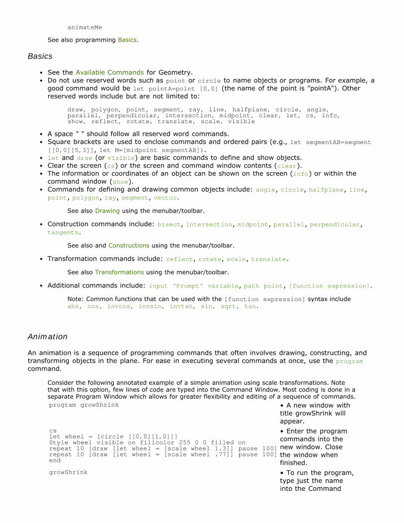
Animation

An animation is a sequence of programming commands that often involves drawing, constructing, andtransforming objects in the plane. For ease in executing several commands at once, use the programcommand.

Consider the following annotated example of a simple animation using scale transformations. Notethat with this option, few lines of code are typed into the Command Window. Most coding is done in aseparate Program Window which allows for greater flexibility and editing of a sequence of commands.program growShrink • A new window with

title growShrink willappear.

cs let wheel = [circle [[0,0][1,0]]]Style wheel visible on fillcolor 255 0 0 filled onrepeat 10 [draw [let wheel = [scale wheel 1.3]] pause 100]repeat 10 [draw [let wheel = [scale wheel .77]] pause 100]end

• Enter the programcommands into thenew window. Closethe window whenfinished.

growShrink • To run the program,type just the nameinto the Command

Window.to growShrink • To edit the program,

type the to commandfollowed by the nameof the program.Alternatively, type theprogram commandfollowed by the nameof the program. TheProgram Window willbe shown.

Geometry & Trigonometry Quick Links:Help Topics Interactive

GeometryAdvanced Apps Commands Index

Geometry & Trigonometry Custom Apps

The Geometry & Trigonometry Custom Apps embed dynamic 2D and 3D shapes and animations. Click onthe name of a tool below for a description and related help topics:

2DPolygons & Transformations

Explore Similar TrianglesExplore SSATilings with Regular PolygonsTilings with Triangles orQuadrilateralsTriangle Congruence

Angles, Arcs, & Measure

Explore Angles and ArcsExplore Radians

Programming & Animation

Design by Robot

3DSlicing a Double Cone Slicing or Unfolding Polyhedra Surface of Revolution

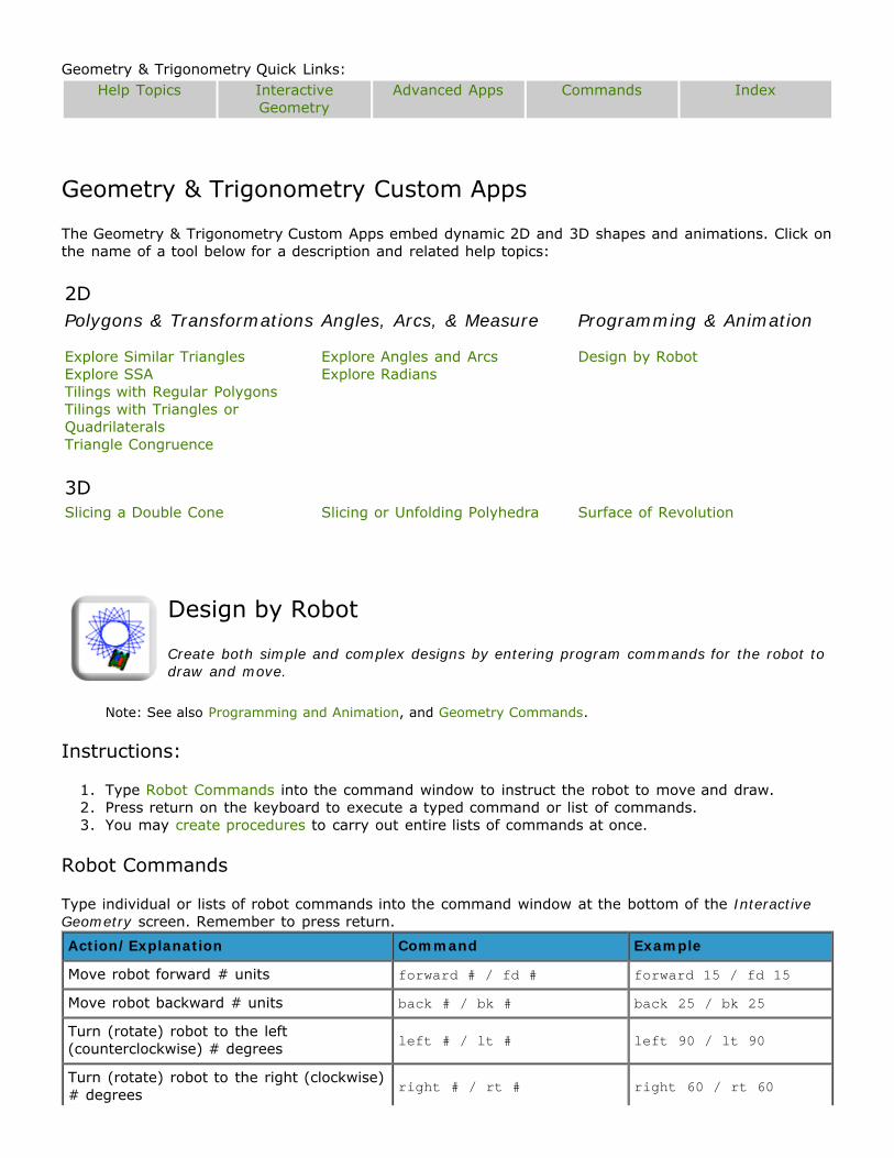
Design by Robot

Create both simple and complex designs by entering program commands for the robot todraw and move.

Note: See also Programming and Animation, and Geometry Commands.

Instructions:

1. Type Robot Commands into the command window to instruct the robot to move and draw.2. Press return on the keyboard to execute a typed command or list of commands.3. You may create procedures to carry out entire lists of commands at once.

Robot Commands

Type individual or lists of robot commands into the command window at the bottom of the InteractiveGeometry screen. Remember to press return.Action/Explanation Command Example

Move robot forward # units forward # / fd # forward 15 / fd 15

Move robot backward # units back # / bk # back 25 / bk 25

Turn (rotate) robot to the left(counterclockwise) # degrees left # / lt # left 90 / lt 90

Turn (rotate) robot to the right (clockwise)# degrees right # / rt # right 60 / rt 60

Put the pen up (do not draw) pu fd 5 pu fd 5 pd fd 5

Put the pen down (draw) pd repeat 2 [rt 90 fd 5pu rt 90 fd 5 pd]

Clear the drawing on the screen (does notmove the position of the robot) cs cs repeat 3 [lt 120 fd

4]pd

Return robot to origin/starting position(does not clear drawing) home fd 8 home rt 90 fd 8

Hide robot ht repeat 5 [rt 72 fd 4]ht

Show robot st st

Repeat a command the desired # of times repeat # [command(s)] repeat 8 [fd 3 rt 45]

Delay the execution of a command by # pause # repeat 3 [fd 10 rt 120pause 500]

Help Tip 1: Put a space between the command and the numerical value(s) associated with thecommand.

Correct Example: fd 15 lt 270

Incorrect Example: fd15lt270

Help Tip 2: If you get an error message such as >I don't know how to ... check the spacing andspelling of your commands; revise and try to execute again.

Help Tip 3: If you get an error message such as >Not enough parameters! check that you have aspace and a numerical value after appropriate commands (see Robot Commands with #'s); revise andtry to execute again.

Help Tip 4: The robot can also do arithmetic. For example, type rt (270-45*2).

Create Procedures

Carry out entire lists of commands at once by creating a procedure.

1. Type to in the command window followed by a single space then nameprocedure.2. Press Enter on the keyboard to execute the script in Step 1. A program window will automatically

open.3. Type in the program window the commands you wish to include in your procedure.4. Close out of the program window by clicking on the X in the upper corner of the window bar.5. Run your procedure by typing nameprocedure in the command window.

Example:

Command Explanation/Result

to squares Type in command window; computerrecognizes the creation of a procedurereferenced by the word or called "squares"

cs home repeat 4 [fd 4 rt 90 pause 550]repeat 4 [fd 8 rt 90 pause 550]

Type in the program window; these are thecommands that the procedure "squares" willcarry out. *Be sure to close out of this windowbefore moving on.

squares Type in the command window; the definedprocedure will automatically be carried out andthe robot will draw two squares.

Explore Angles and Arcs

Explore the relationship between the measures of inscribed angles and their interceptedarcs.

Instructions:

1. Drag point B.2. Click the "Show Measures" button to show the measures of angle ABC, angle AOC, and arc AC.

Click "Hide Measures" to hide these measures.3. Drag points A and C to consider right angle ABC and obtuse angle ABC.

Explore Radians

Experiment measuring angles in radians and how radian measures are related to degreesand revolutions.

Instructions:

1. Decide upon a target. Options for entering a target include:Click on one of the "Enter Target in..." buttons for Degrees, Revolutions, or Radians. Type avalue into the message window (type "PI"), then click Done. The target will move along thecircle according to the specified value.Click on the "Random Target" button. The target will move along the circle to a randomlocation.Drag the target along the circle.

2. Guess the target value. Click on one of the "Guess..." buttons for Degrees, Revolutions, orRadians. Type your guess into the message window, then click Done. To end the guess process,click Cancel.

3. Choose the "Show Measurements" button to display measures for the measure of angle BOT indegrees and radians, length of segment OB, and arclength of arc BOT. Click "Hide Measurements"to hide these values.

Explore Similar Triangles

Investigate the construction of pairs of similar triangles by applying the definition ofsimilar triangles.

Instructions:

1. Select a scale factor by dragging point K along the slider between the values of 0 and 6.2. Drag points D, E, and F so that triangle DEF is similar to triangle ABC.3. Click the "Test if Similar" button to test if the two triangles are indeed similar. If so, the actual

scale factor will be displayed above the target scale factor. If not, you will be prompted to go backto Step 2.

4. Once the triangles are similar, the program will create triangle A'B'C' for comparison to triangle

DEF. An animation of this transformation process will be displayed. Specifically, triangle ABC willbe scaled by a scale factor of K, then translated, rotated, and reflected (as needed) until triangleA'B'C' coincides with triangle DEF.

5. Drag point K to observe how various scale factors for triangle A'B'C' compare to the actual scalefactor relating triangles ABC and DEF.

6. Click the "New Triangles" button to generate a new case for investigation.

Explore SSA

Experiment with various side and angle measures to explore the Side-Side-Anglecongruence condition for triangles.

Instructions:

1. Drag the red points to change the measure of angle A, or side lengths AB and BC.2. To guide your investigation you may wish to determine for which measurements or intervals of

measurement the given side-side-angle parts determine no triangle, exactly one triangle, twononcongruent triangles.

Slicing a Double Cone

Dynamically manipulate a plane slicing a double cone and view the corresponding conicsection.

Conic sections are defined as the intersection of a plane and a right circular double cone. This customapp allows for the manipulation of the position of the plane (drag the tilt slider) and the view of thedouble cone (drag the cone itself) in order to examine the resultant intersection. The help topics belowinclude information on: Slicing Plane Attributes and the Tool Menu.

Slicing Plane Attributes

Tilt (Angle from xy-plane): The tilt angle is determined by the angle formed between the xy-planeand the shaded plane shown. Notice that the 2D rendition of the angle and the conic sectiondynamically update as the tilt is changed.

Note: To adjust the Settings, choose the red box to view the Configuration Panel in order toset minimum and maximum values for the tilt angle. Unit and block increments can also beadjusted. Click OK to make these changes or Cancel to exit without change.

Vertical Translation: Drag the horizontal slider bar to adjust the vertical translation of the planethat cuts across the double-cone.

Note: To adjust the Settings, click the red box to set minimum and maximum values for thevertical translation of the plane. Unit and block increments can also be adjusted. Click OK tochange these settings or Cancel to exit without change.

Choose Wire Frame from the Options menu to show the frame of the double cone instead of theshaded surface.

Choose Label Conic from the Options menu to show labels of the type of conic section shown onboth the 3D View and the Standard View.Choose Extend Double Cone or Shrink Double Cone from the Options menu to adjust the size ofthe double cone in the 3D View.

Tool menu

The Tool menu offers options to Restart, Print, and Close the custom app.

Choose Tool | Restart to reset the viewing window to the original display.Choose Tool | Print to print the current view of the slice.

See also Save & Print.

Choose Tool | Close or the X button to close this custom app.

Slicing or Unfolding Polyhedra

Visualize common polyhedra and manipulate 3D modeling options such as cutting andunfolding.

Instructions

1. Set up the model by choosing a solid from the Polyhedron menu.2. Adjust the graph view.

Click and drag the shape on the screen to rotate it in the 3D space.It might be helpful to adjust the transparency of the shape before manipulating.Choose to View | Zoom In , Zoom Out , and Zoom Fit .The Vertices, Edges, and Faces of a solid can be shown or hidden by selecting (ordeselecting) them in the View menu.

3. Model the slicing or unfolding of the selected polyhedra.Choose Enable in the Cut, Unfold, or Transform menus.Drag the available slider bars to adjust the model accordingly

4. Use the Tool menu to save, print, or otherwise record your work.

See also Save & Print.

Surface of Revolution

Draw and manipulate a line or connected series of line segments in two-dimensionalspace to simultaneously generate a surface of revolution in three-dimensional space.

A surface of revolution is a surface formed by rotating (revolving) a curve about a line. The help topicsbelow include information on: the Draw Tools for defining lines and curves, the Revolution Settings forsetting the angle and axis of revolution, the Tool menu, and Options menu.

Draw Tools

Choose to Clear All in the current drawing(s) and reset the axis to the original position.Alternatively, choose Tool | Restart to obtain the original starting view, settings, and graph.

Choose the Draw tool to define a new curve or line. Click and release the mouse over the 2Dcoordinate grid to define points. Points will automatically be connected with a segment to the pointpreceding it. Another drawing technique is to click and drag as you hold the mouse button down.

Dynamic Drawing: Notice that as points are drawn on the coordinate grid, the surface ofrevolution is correspondingly defined in the three-dimensional space.

Use the Select tool to click on and drag defined points to new locations on the coordinate grid.Observe how the 3D surface of revolution automatically updates.

Revolution Settings

Angle of Rotation: Drag the slider bar as the angle of rotation for the surface of revolution isdynamically updated.

Note: The default setting for the angle of rotation is 180° and ranges from 0° to 360°. Clickthe red box to the right of this slider bar to set different minimum and maximum values, andindicate the unit and block increment. Click OK to update the settings or Cancel to exit withoutchanging the settings.

Axis of Rotation: Choose the or buttons to change the axis of rotation to the y- or z-axis,respectively.

Tool menu

The Tool menu offers options to Restart, Print, and Close the custom app.

Choose Tool | Restart ( ) to obtain the original starting view, settings, and graph.Choose Tool | Print to print the currently selected frame.

See also Save & Print.

Choose Tool | Close or the X button to close this custom ap. Return to the main screen to make anew tool selection.

Options menu

The Options menu allows you to modify the display of the 3D surface of revolution.

Choose Options | Show Edges to toggle the wireframe of the surface of revolution.Select Options | Show Surface to toggle the quadrilateral faces that comprise the surface ofrevolution.Choose Options | Show Meridian to toggle the 2D curve used to sweep out the surface ofrevolution.Choose Options | Show 3D Axes to toggle the x-y-z coordinate axes.Choose Options | Rotate about Horizontal Axis or the button to perform the revolution aboutthe y-axis rather than the z-axis.Choose Options | Rotate about Vertical Axis or the button to perform the revolution about thez-axis rather than the y-axis.

Tilings with Triangles or Quadrilaterals

Explore tiling the plane with triangles or quadrilaterals using rotations of 180 degreesabout midpoints of sides.

Instructions:

1. In the Shape menu, choose to tile using Triangles or Quadrilaterals. You may change the shape atany time.

Note: Only one shape may be used at a time and if you choose a new shape it will clear andreplace the current drawing.

2. Drag any vertex to change the shape of the figure.3. Click on or near the midpoint of an edge of the figure. This rotates a copy of the figure 180°

about the midpoint of the edge and attaches the rotated copy to that edge.4. Repeat Step 3 several more times – at least until you have completely surrounded the original

figure including all of its vertices with copies of the figure.5. As you build a tiling, you may need to know:

Remove the last polygon placed by choosing Undo in the Edit menu or the button on thetoolbar.Clear the current drawing and start over by choosing Restart in the Tool menu, Clear in theEdit menu, or the button on the toolbar.Change (or turn off) the rotation animation by choosing Fast, Slow, or Off in the Edit menuunder the sub-option Animation.Print the current tiling by choosing Print in the Tool menu or the button on the toolbar.

Tilings with Regular Polygons

Explore tiling the plane with regular polygons to create regular and semiregulartessellations.

Instructions

1. Choose the number of sides of the regular polygon that will be placed next by clicking on thebutton to the left of that number at the top of the window.

2. Click anywhere in the blank window to place the first polygon.3. To attach a new polygon to one already placed, choose the number of sides (see Step 1) then

click near the edge of the polygon to which you want it attached.

Remember: As you build the tiling, there should be no gaps and no overlaps.

4. As you attach more and more polygons to build a tiling, you may need to know:Remove the last polygon placed by choosing Edit | Undo or the button on the toolbar.Delete a polygon by clicking in the center of it then choosing Edit | Delete Polygon or the button.Scale the tiling (make it larger or smaller) by using the Zoom slider.Clear the current drawing and start over by choosing Tool | Restart, Edit | Clear, or the button.Print the current tiling by choosing Tool | Print or the button on the toolbar.

See also Save & Print.

Original applet written by Melinda Green and Don Hatch, modified by S. Keller.

Triangle Congruence

Explore combinations of side or angle measures that determine the existence of a uniquetriangle (or the congruence of two triangles). Test for congruence with measurements oran animated transformations approach.

Instructions:

1. Select a possible condition for congruence of triangles from the "Select a Condition" drop-downmenu.

Options include: Side-Angle-Side, Side-Side-Angle, Angle-Side-Angle, and Side-Side-Side.

2. Angle/side measures will be generated for you and these measures determine the figure drawn onthe screen.

You may choose to enter your own side/angle measures by typing values into the boxes to theright of the drop-down menu. Be sure to press Enter to construct a triangle with these fixedmeasures.

Alternatively, click the button for the Custom App to generate a different set of measuresfor you.

3. With the desired fixed measures set, try to build a triangle by dragging the blue colored verticesand/or the lengths of the ray(s).

4. The labels of the triangle vertices (A, B, and C) will automatically appear on the screen when atriangle has been formed.

Note: Choose Options | Show Measurements to display the remaining side and anglemeasures of the constructed triangle.

5. If possible, create a second triangle with the same set of chosen measures by repeating Steps 3and 4.

6. Compare the measurements and/or shape and size of the two formed triangles. Are the trianglescongruent?

To test by transformations, choose the button to play the first step in a sequence oftransformations. Continue until the triangles coincide (if possible). Choose the to resetthe triangle positions and test again.

Use the Options menu to customize the ways triangles are created and tested to becongruent. For instance, show the transformations as a step through sequence oranimation.

Use the Test by Transformations menu to specify the sequence of transformations thatis performed. For instance, use only reflections or a sequence of reflections.

Move the second formed triangle (shaded in red) until it coincides with the first by clickingand dragging. Dragging from the center of the figure will move its positions on the screen,dragging from a vertex will rotate it about that vertex. Additionally, use the button orsimply double-click on one of the triangles to reflect it.

7. Repeat Steps 2-6 several more times until you have a few cases for your chosen condition.

Geometry & Trigonometry Quick Links:Help Topics Interactive

GeometryCommands Custom Apps Catalog

Geometry & Trigonometry Index

All help topics and commands that are available within the Geometry & Trigonometry strand of tools arelisted below in alphabetical order.

[abs number]Add VectorsAngle, angleAngle MeasureAngle BisectorAnimationAreabisectCalculate, CalculationChange Style of SelectedCircle, circleCircumferenceclearCommand WindowConstructionsCoordinatesCoordinate Geometry[cos number] csCustom AppsDelete SelectedDefault SettingsDefault StylesDesign by RobotDraw, drawEdit menuExplore Angles and ArcsExplore RadiansExplore Similar TrianglesExplore SSA

Figure or PolygonFilled, Fill ColorFont[function expression]Grid StyleHalf Plane, halfplaneHide CoordinatesHide Selectedinfoinput "Prompt" variableIntersection, intersection[invcos number] [invsin number][invtan number]LabelsLengthsletLine, lineList of ShapesMeasureMenubarMidpoint, midpointOptions menuParallel, parallelpath pointPerimeterPerpendicular, perpendicularPoint, pointPolygon, polygonprogramProgrammingRay, rayReflect, reflect

Rotate, rotateScale, scaleSegment, segmentSelectshowShow CoordinatesShow Hidden[sin number]Slicing a Double ConeSlicing or Unfolding PolyhedraSlopesSnap to Grid [sqrt number]Style WindowSurface of RevolutionSynthetic Geometry[tan number]Tangents, tangentsThicknessTilings with Regular PolygonsTilings with Triangles orQuadrilateralsToolbarTransformationsTranslate, translateTriangle CongruenceUndoVector, vectorVisible, visibleWindow Scale

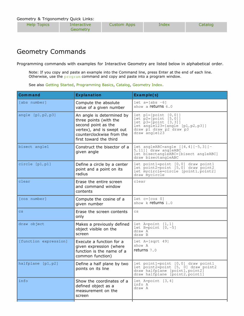
Geometry & Trigonometry Quick Links:Help Topics Interactive

GeometryCustom Apps Index Catalog

Geometry Commands

Programming commands with examples for Interactive Geometry are listed below in alphabetical order.

Note: If you copy and paste an example into the Command line, press Enter at the end of each line.Otherwise, use the program command and copy and paste into a program window.

See also Getting Started, Programming Basics, Catalog, Geometry Index.

Command Explanation Example(s)

[abs number] Compute the absolutevalue of a given number

let a=[abs -6]show a returns 6.0

angle [p1,p2,p3] An angle is determined bythree points (with thesecond point as thevertex), and is swept outcounterclockwise from thefirst toward the third

let p1=[point [0,0]]let p2=[point [5,0]]let p3=[point [3,3]]let angle123=[angle [p1,p2,p3]]draw p1 draw p2 draw p3draw angle123

bisect angle1 Construct the bisector of agiven angle

let angleABC=angle [[4,4][-5,3][-5,11]] draw angleABClet bisectangleABC=[bisect angleABC]draw bisectangleABC

circle [p1,p1] Define a circle by a centerpoint and a point on itsradius

let point1=point [0,0] draw point1let point2=point [5,0] draw point2let mycircle=circle [point1,point2]draw mycircle

clear Erase the entire screenand command windowcontents

clear

[cos number] Compute the cosine of agiven number

let c=[cos 0]show k returns 1.0

cs Erase the screen contentsonly

cs

draw object Makes a previously definedobject visible on thescreen

let A=point [1,1]let B=point [0,-5] draw Adraw B

[function expression] Execute a function for agiven expression (wherefunction is the name of acommon function)

let A=[sqrt 49]show A returns 7.0

halfplane [p1,p2] Define a half plane by twopoints on its line

let point1=point [0,0] draw point1let point2=point [5, 0] draw point2draw halfplane [point1,point2]draw halfplane [point2,point1]

info Show the coordinates of adefined object as ameasurement on thescreen

let A=point [3,4]info Adraw A

input "Prompt"variable

Call an input window andgive a value to thevariable "Prompt"

input "Prompt" variable returns a window,type 5, Done.

intersection object1object2

Define the intersection oftwo previously definedobjects

let lineAB=line [[3,0][8,5]]let lineCD=line [[0,0][5,-3]]let E=[intersection lineAB lineCD]draw lineAB draw lineCD draw E

[invcos number] Compute the inversecosine of a given number

let ic=[invcos 1]show ic returns 0.0

[invsin number] Compute the inverse sineof a given number

let is=[invsin 0]show is returns 0.0

[invtan number] Compute the inversetangent of a given number

let it=[invtan 0]show it returns 0.0

let Define and name objectsfor use, the charactersthat follow the letcommand represent thename of the object

let origin=point [0,0]draw origin

line [p1,p2] Define a line by two points let point1=point [0,0] draw point1let point2=point [5,0] draw point2let line1=line [point1,point2]draw line1

midpoint object1 Construct the midpoint ofan object (e.g., a segmentor polygon)

let AB=[[-7,7][13,1]]let CD=[[3,8][3,2]]let M=[midpoint AB] show coord M

parallel point1 line1 Determine a parallel linethrough a given point to agiven line

let line1=line [[0,0][1,1]]let point1=point [-2,0] draw line1draw point1let line2 =[parallel point1 line1]draw line2

path pointpath point point

Determine the path of agiven point

let P=[point [0,0]]drag point P on the screen to a new locationthenshow path point P> pathpoint[3.0, -9]

perpendicular point1line1

Determine a perpendicularline through a given pointto a given line

let line1=line [[0,0][1,1]]let point1=point [-2,0] draw line1draw point1let line3=[perpendicular point1 line1]draw line3

point [x,y] Define a point determinedby an ordered pair insquare brackets [x-coordinate, y-coordinate]

let A=[point [2,7]]draw A

polygon [p1,p2,...,pn] Determine a polygon orshape by a finite numberof points

let R=point [2,7]let S=point [0,0]let T=point [-2,-2]let shapeRST=polygon [R S T]draw R draw S draw Tdraw shapeRST

program Type the programcommand (followed by aspace and the name ofyour program) into theCommand Window to workwithin the Program Editor.Close this window then callthe program by typing its

program animateMe(type program into programming window,then close window) animateMe

name.

ray [tail,head] Define a ray by a tail anda head

draw ray [[5,0],[8,6]]

reflect object1,line1 Reflect a previously definedobject over a previouslydefined line

let A=point [4,4] let B=point [7,12]let C=point [-1,2]let lineDE=line [[5,4][10,4]]let triangleABC=polygon [A B C]let A'=[reflect A lineDE]let B'=[reflect B lineDE]let C'=[reflect C lineDE]let triangleA'B'C'=polygon [A' B' C']draw A draw B draw Cdraw triangleABCdraw lineDEdraw A' draw B' draw C'draw triangleA'B'C'

rotate object1 angle1 Rotate an object to berotated by a specifiedangle (either numerical oras a defined object)

let triangleABC=polygon [[4,5][1,7][4,-2]]draw triangleABCdraw rotate triangleABC 45

scale object1 vector1scale object1scalefactor

Scale an object by a vectoror scale factor, centered atthe origin

let A=point [-6,6]let B=point [-8,0]let C=point [-3,4]let triangleABC=polygon [A B C]let A'B'C'=[scale triangleABC 1.5]draw triangleABC draw A'B'C'

segment [p1,p2] Define a segment by twoendpoints

let segAB=[segment [[0,0],[5,0]]]draw segAB

show Show the coordinates of adefined object within thecommand window

let segAB=[segment [[0,0],[5,0]]]let M=[midpoint segAB]show M

[sin number] Compute the sine of agiven number

let s=[sin 0]show s returns 0.0

[sqrt number] Compute the square rootof a given number

let k=[sqrt 57]show k returns 7.5498344

[tan number] Compute the tangent of agiven number

let t=[tan 0]show t returns 0

tangents circle1 point1 Construct tangents to acircle through a point on oroff the circle

let A=point [-9,5] let B=point [-4,9]let circleAB=circle [A B]draw A draw B draw circleAB let tcircleABB=[tangents circleAB B]draw tcircleABB

translate object1vector1

Translate an object by atranslation vector (eitheran ordered pair or as adefined object such as asegment).

let A=point [-6, 6]let B=point [-8, 0]let C=point [-3, 4]let triangleABC=polygon [A B C]let seg1=segment [[0,0][5,0]]let imag1=[translate triangleABC [8,0]]let imag2=[translate triangleABC seg1]draw triangleABC draw imag1 draw imag2

vector [tail,head] Define a vector by a tailand a head

draw vector [[-2,0],[-3,3]]

visible together with the stylecommand, make an objectvisible or hidden with "on"or "off"

let object=[segment [[-5,1][5,2]]]style object visible on

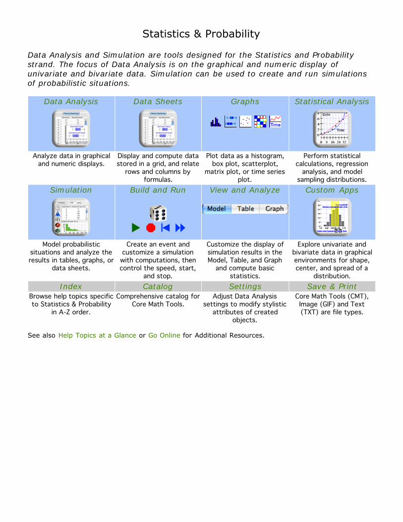
Statistics & Probability

Data Analysis and Simulation are tools designed for the Statistics and Probabilitystrand. The focus of Data Analysis is on the graphical and numeric display ofunivariate and bivariate data. Simulation can be used to create and run simulationsof probabilistic situations.

Data Analysis Data Sheets Graphs

Statistical Analysis

Analyze data in graphicaland numeric displays.

Display and compute datastored in a grid, and relate

rows and columns byformulas.

Plot data as a histogram,box plot, scatterplot,

matrix plot, or time seriesplot.

Perform statisticalcalculations, regression

analysis, and modelsampling distributions.

Simulation Build and Run

View and Analyze Custom Apps

Model probabilisticsituations and analyze theresults in tables, graphs, or

data sheets.

Create an event andcustomize a simulationwith computations, thencontrol the speed, start,

and stop.

Customize the display ofsimulation results in theModel, Table, and Graph

and compute basicstatistics.

Explore univariate andbivariate data in graphicalenvironments for shape,center, and spread of a

distribution.Index Catalog Settings Save & Print

Browse help topics specificto Statistics & Probability

in A-Z order.

Comprehensive catalog forCore Math Tools.

Adjust Data Analysissettings to modify stylistic

attributes of createdobjects.

Core Math Tools (CMT),Image (GIF) and Text(TXT) are file types.

See also Help Topics at a Glance or Go Online for Additional Resources.

Statistics & Probability Quick Links:Help Topics Data Sets Custom Apps Index Save & Print

Data Analysis

Use the Data Analysis tool to analyze univaritate and bivariate data in graphical and numeric displays.

A Data Analysis data sheet is like aspreadsheet environment with statisticsrelated functionality.

Data

To modify or edit a pre-loaded data set, choose Edit | Enable.

Choose a data set from the Data menu for quick access to pre-loaded data examples.

See also Data Sets, Spreadsheet.

Edit Styles and Settings

Help topics for Edit menu options including Cut, Copy, Paste, Fill Down, Set # of Digits, Column Name,and Column Formula are common across Spreadsheet and Data Analysis.

Note: Some functionality is available within Spreadsheet and not in Data Analysis (e.g., Sort, Deleteand Insert rows/columns).

Note: Settings for graphs are available within the Options menus once a plot is shown.

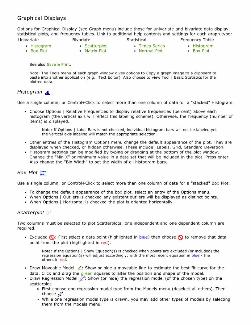
Graphical Displays

Options for Graphical Display (see Graph menu) include those for univariate and bivariate data display,statistical plots, and frequency tables. Link to additional help contents and settings for each graph type:Univariate Bivariate Statistical Frequency Table

HistogramBox Plot

ScatterplotMatrix Plot

Times SeriesNormal Plot

HistogramBox Plot

See also Save & Print.

Note: The Tools menu of each graph window gives options to Copy a graph image to a clipboard topaste into another application (e.g., Text Editor). Also choose to view Tool | Basic Statistics for theplotted data.

Histogram

Use a single column, or Control+Click to select more than one column of data for a "stacked" Histogram.

Choose Options | Relative Frequencies to display relative frequencies (percent) above eachhistogram (the vertical axis will reflect this labeling scheme). Otherwise, the frequency (number ofitems) is displayed.

Note: If Options | Label Bars is not checked, individual histogram bars will not be labeled yetthe vertical axis labeling will match the appropriate selection.

Other entries of the Histogram Options menu change the default appearance of the plot. They aredisplayed when checked, or hidden otherwise. These include: Labels, Grid, Standard Deviation.Histogram settings can be modified by typing or dragging at the bottom of the plot window.Change the "Min X" or minimum value in a data set that will be included in the plot. Press enter.Also change the "Bin Width" to set the width of all histogram bars.

Box Plot

Use a single column, or Control+Click to select more than one column of data for a "stacked" Box Plot.

To change the default appearance of the box plot, select an entry of the Options menu.When Options | Outliers is checked any existent outliers will be displayed as distinct points.When Options | Horizontal is checked the plot is oriented horizontally.

Scatterplot

Two columns must be selected to plot Scatterplots; one independent and one dependent column arerequired.

Excluded : First select a data point (highlighted in blue) then choose to remove that datapoint from the plot (highlighted in red).

Note: If the Options | Show Equation(s) is checked when points are excluded (or included) theregression equation(s) will adjust accordingly, with the most recent equation in blue - theothers in red.

Draw Moveable Model : Show or hide a moveable line to estimate the best-fit curve for thedata. Click and drag the green squares to alter the position and shape of the model.Draw Regression Model : Show (or hide) the regression model (of the chosen type) on thescatterplot.

First choose one regression model type from the Models menu (deselect all others). Thenchoose .While one regression model type is drawn, you may add other types of models by selectingthem from the Models menu.

The most recently drawn regression model is colored in blue and all previously drawnregression models are in red.

Note: Regression models are not moveable, but will be reformulated and drawn if points areremoved/excluded (or re-included).

See also Moveable Model.

Draw Residuals : Show (or hide) the residuals for a drawn moveable model ( ) and the mostrecently drawn regression model ( ). At least one regression model or a moveable line must bedrawn for residuals to be plotted.

See also Statistics | Regression, Models | Analysis.

Draw Squares : Show (or hide) the squares of the residuals for a drawn moveable model ( )and the most recently drawn regression model ( ). At least one moveable model or a moveableline must be drawn for squares to be plotted.

See also Error Thermometer.

Draw Means : Show (or hide) horizontal and vertical lines representing the x and y means forthe plotted data. Move the mouse cursor over the intersection of these red lines to give theordered pair of the means.

Note: If a data point is excluded ( ) the means will adjust accordingly.

Choose Options | Show Equations to show (or hide) the equations of any drawn moveable orregression models on the scatterplot. The equations will be colored-coded to match the model theyrepresent.Select Options | Show Predicted Value(s) to show (hide) a table of predicted values correspondingto all drawn regression ( ) and moveable ( ) models in a separate window. At least oneregression model or a moveable line must be drawn for residuals to be plotted. Click on a tableentry and use the arrow keys on your keyboard to move through the table of values; notice thecorresponding point and coordinates are highlighted in the scatterplot window.

Note: The range of x values that are used within the scatterplot window will be used by defaultfor the Predicted Values window. Type numerical values into the Min x, Max x, and x Stepboxes and press Enter after typing in each box to change these settings.

Choose Options | Error Thermometer to show (or hide) a depiction of the sum of the squarederrors (SSE) for the drawn models to the right of the scatterplot. This option is useful whencomparing the SEE of the moveable model with the SEE of the regression model.

See also Draw Squares.

Guess Correlation : Show (or hide) the guess correlation bar to the right of the scatterplot.Select a guess for r from one of the five options available then click Show r to view the actualcorrelation value.

Note: Although you can calculate a correlation for any scatterplot, r measures only straight-line(linear) relationships.

Plot Information : Show (or hide) scatterplot information. Options include those for modifyinglabels for x and y, viewing basic statistics for the plotted data, naming the plot (or title), andadjusting window settings. Additionally, you may check options to Show Correlation, Show SEE,and Show Confidence Bands.The Scatterplot | Models menu allows you to select (or deselect) the type of model that is drawnon a scatterplot. The chosen model applies to both Moveable ( ) and Regression ( ) models.Choose Models | Enter/Edit a Model to type your own model type in "y = ..." form. If such amodel has already been drawn, choosing this menu option will allow you to edit the previously-entered model.

Note: The program will not accept your model if you type "y=" in the Enter/Edit a Modelwindow. Instead, enter the rest of the model, without the "y=" then click OK.

Analysis : Analyze a plot of the independent variable and the plot of residuals in a separatewindow. Within this Residual Plot(s) window:

The Tool menu gives options to view Basic Statistics, Print, or Save the residual analysis.Choose an entry from the Options menu to change the view of the residual plot. The defaultview of Residual vs. X is selected, when other options are selected they will be added to theright of the original selection. Menu entries include: Residuals vs. X, Residuals vs. Y,Residuals vs. Order, Normal Probability Plot, and Regression Analysis.

Matrix Plot

Two or more columns must be selected to plot a Matrix Plot.

Time Series

At least one column of data must be selected to plot a Time Series graph (multi-column graphs will becolor-coded).

Normal Plot

At least one column of data must be selected to plot a Normal Plot graph (multi-column graphs will becolor-coded).

Frequency Table | Histogram, Box Plot

There are two options for frequency tables: Histogram, and Box Plot. To use these plot options, thevalues of frequency table should be listed in one column, with their corresponding frequencies in anothercolumn.

Statistical Analysis

Descriptive Statistics

Choose Statistics | Descriptive Statistics to view summary statistics for the columns of an active datasheet. The following calculations are given for each column:

n (number of values in the column), Mean (arithmetic average), Minimum (smallest value), Q1 (firstquartile), Median (middle value of ordered list), Q3 (third quartile), Maximum (largest value), SampleStandard Deviation (a measure of spread), Sample Variance (the square of the standard deviation).

Chi-Square Test

To use the Chi-Square Test:

1. First open or create your own bivariate categorical data set (e.g., Crying).2. Choose Statistics | Chi-Square Test to open a Chi-Square Analysis window to obtain the chi-

squared statistic.Use the Tests menu and choose to Test for Independence, Test for Homogeneity, ordetermine a Goodness of Fit.Use the Options menu to Show Expected Counts, Show Expected Percents, or Show CriticalValues.

Randomization Distribution

Create an approximate sampling distribution of possible differences in means, medians, or standarddeviations of two treatments by rerandomizing, then identify extreme events.

See Statistics & Probability Custom Apps.

Distribution of Sample...

Explore the shape, mean, and standard deviation of distributions of sample means, medians, or standarddeviations for various sample sizes.

See Statistics & Probability Custom Apps.

Regression

Within an open data set, choose a regression type (e.g., linear) from the Statistics menu. Within theChoose Columns window, select one column for each of the independent and dependent variables. ClickOK to approve the choices and view the Regression Analysis Frame. Several options are available withinthis frame:

The Results tab lists all regression statistics for the chosen regression type (e.g., Linear) including:Sample Statistics, Coefficient Estimates, 95% Confidence Intervals, and Analysis of Variance.The Graph tab shows a scatterplot of the data along with the chosen regression model, shown inred. The regression equation is shown above the graph.The Residuals tab shows a plot of the residuals on the scatterplot of the data. A time series plotof the data is also shown within this tab.

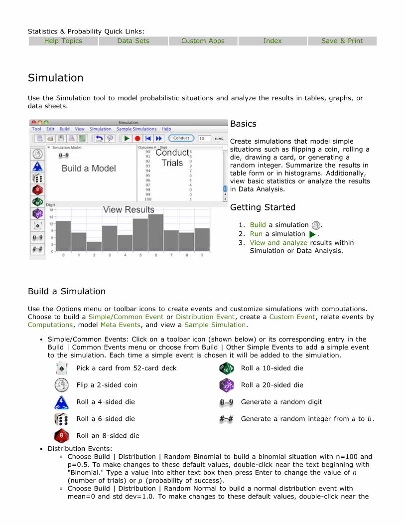
Statistics & Probability Quick Links:Help Topics Data Sets Custom Apps Index Save & Print

Simulation

Use the Simulation tool to model probabilistic situations and analyze the results in tables, graphs, ordata sheets.

Basics

Create simulations that model simplesituations such as flipping a coin, rolling adie, drawing a card, or generating arandom integer. Summarize the results intable form or in histograms. Additionally,view basic statistics or analyze the resultsin Data Analysis.

Getting Started

1. Build a simulation .2. Run a simulation .3. View and analyze results within

Simulation or Data Analysis.

Build a Simulation

Use the Options menu or toolbar icons to create events and customize simulations with computations.Choose to build a Simple/Common Event or Distribution Event, create a Custom Event, relate events byComputations, model Meta Events, and view a Sample Simulation.

Simple/Common Events: Click on a toolbar icon (shown below) or its corresponding entry in theBuild | Common Events menu or choose from Build | Other Simple Events to add a simple eventto the simulation. Each time a simple event is chosen it will be added to the simulation.

Pick a card from 52-card deck Roll a 10-sided die

Flip a 2-sided coin Roll a 20-sided die

Roll a 4-sided die Generate a random digit

Roll a 6-sided die Generate a random integer from a to b.

Roll an 8-sided die

Distribution Events:Choose Build | Distribution | Random Binomial to build a binomial situation with n=100 andp=0.5. To make changes to these default values, double-click near the text beginning with"Binomial." Type a value into either text box then press Enter to change the value of n(number of trials) or p (probability of success).Choose Build | Distribution | Random Normal to build a normal distribution event withmean=0 and std dev=1.0. To make changes to these default values, double-click near the

text beginning with "Normal." Type a value into either text box then press Enter to changethe value of the mean or standard deviation.

Custom Events: Choose Build | Create Custom Event and double-click the "unnamed" event in thesimulation window. Name the event and specify the desired outcomes. Enter a frequency or weightfor each outcome. Close the window when finished.

Choose Edit | Add Outcome or Edit | Delete Outcome to create more or fewer outcomes.Choose Edit | Make Equally Likely to give all outcomes the same frequency or weight.

Computations: To relate events by a computation first build them so they are added to thesimulation model. Next, hold down the shift key as you click to and select the desired events.Choose a computation from the Build menu such as Add, Subtract, Equal, or Combine, or from theAdditional Computations entry to relate the selected events.

Example 1. Choose then then . Click on and hold down shift to select , thenchoose Build | (Computations) Add. A new event will be created that will read + (8-sidedDie + 4-sided Die). The outcome for this combined event will add the value of the 8-sided Dieto the value of the 4-sided Die for each run of the simulation.

Example 2. Choose three times. Hold down the Shift key as you click on each of the digiticons ( ) within the model window. With this selection highlighted, choose Build | AdditionalComputations | Function. A separate Function Editor window will open describing how each ofthe selected events are coded (e.g., a:Digit, b:Digit, c:Digit). To relate these events by afunction that computes their mean, type (a+b+c)/3 and press Enter (or type average(a,b,c)).A new event that relates the three random digits is listed in the simulation model. Expand orcollapse the view (click on the small triangle to the left of the function) to determine whichresults are displayed in the table and graph.

Meta Events: To create a Meta Event, first build a simple or custom event so that it is added tothe simulation model. Click on the desired event to select it. With the event selected, choose fromBuild | Meta Events | Accumulate Total, Proportion of, Count Till See, or Count # of.

Note: Only one Meta Event may be chosen at a time.

Example. Choose , then Build | (Meta Events) Count Till See. Double-click on the outcomethat you are waiting for (this is simulating a waiting-time situation). If you would like to waitfor multiple outcomes from one simulation, hold down the Command key and select multipleoutcomes.

Sample Simulations: View a pre-set simulation by selecting it from the Sample Simulations menu.

Note: When an option from the Sample Simulations menu is chosen it will replace any currentsimulations. Open a new Simulation window to model multiple situations as separatesimulations.

Run a Simulation

After setting up a simulation, use the Simulation menu or their corresponding toolbar buttons to run it.

Choose to start and stop running the simulation.To set the speed of the simulation, select Step, Slow, Medium, Fast, or Fastest in the Simulationmenu. Alternatively, the simulation will run one pace faster with each click of the button.

Note: If the speed is set at a Step pace, click the Go button for each new run.

Choose to reset or clear all performed runs of the simulation, keeping the same set up orbuild.

Note: To clear the build of the simulation choose the button or choose Tool | New.

Use the Conduct button to do a specified number of runs at once. Each click of the Conduct buttonwill add the specified amount to the total number of performed runs.

Note: The Conduct button does not have an effect on the controls that start, stop, anddetermine the speed of the runs.

Choose Edit | Undo to reverse the last action that was performed.

View & Analyze Results

Once your simulation has finished running view or analyze the results.

Viewing Styles and Options

Select (or deselect) entries of the View menu to customize what and how the results of a simulation areshown.

Choose View | Stacked to display the results in separate tabs. Choose View | Tiled to displayresults in one window.From the View menu, choose from three components of a simulation to view: the Model or buildof the simulation, a Table of Outcomes, and a Histogram of results.

Note: A simulation must be built prior to running it (and both must be done before results willbe recorded in the table or graph).

When a histogram plot is shown, use the View menu to show (or hide): Relative Frequencies (orfrequencies), Labels on histogram bars, or a Grid.

Note: Be sure Graph is selected (checked) within the View menu for these settings to beapplied.

Analyze Results

Choose Edit | Basic Statistics to view the available summary statistics of the simulationoutcome(s) in a separate window. These summary statistics include the five-number summary,mean, sample standard deviation, and sample variance.Choose Edit | Analyze Results to view the outcome(s) of the simulation within a Data Analysisdata sheet.

Save and Record Simulations

The Tool menu provides options for creating new simulations ( ), opening saved simulations ( ),printing ( ), and saving ( ).

See also Save & Print.

Statistics & Probability Quick Links:Help Topics Data Analysis Simulation Data Sets Index

Statistics & Probability Custom Apps

The Custom Apps for Statistics & Probability include those for exploring center and spread of univariatedata, investigating regression of bivariate data, and randomization and sampling of various distributions.Click on the name of a tool below for a description and help topics:

Univariate Center andSpread Bivariate Regression Sampling Distributions

Estimate CenterEstimate Center and Spread

Modeling Binomial DistributionsDistribution of SampleRandomization Distribution

Binomial Distributions

Vary the number of successes and the probability of a success on each trial to see howthe shape, center, and spread of binomial distributions are affected. Conduct trials andcompare theoretical models of distributions to simulation results.

Instructions

Upon opening the custom app, a binomial distribution based on sliders for n (number of trials) and p(probability of success) is shown. The theoretical binomial model for the parameter values (default:n=50, p=0.5) is displayed in red. The following provide guidelines and tips on how to utilize thecapabilities of this custom app:

1. Set up additional binomial situations2. Customize display settings (optional)3. Run simulation4. Tool menu options

Set Up Additional Binomial Situations

Add menu

Select entries from the Add menu to consider multiple distributions at the same time. Values for n and pare recorded above each distribution as they are added.

Help Tip: Once a distribution is added, distinguish between those that are controlled by sliders andthose that are editable by noting the colors of values for n and p. In particular, values in gray arecontrolled by the sliders and automatically update the distribution as sliders are dragged. White textboxes with black text are editable - first click on the desired one, type an appropriate value, thenpress Enter to change the corresponding distribution. Editable parameters are not affected by slidersand vice versa.

Choose Add | Sample Grid to replace any current distributions with a 3-row, 2-column grid of 6distributions. Each distribution has editable values for both n and p. Use the Undo button toremove the last distributions, or select from other Add menu entries to add to the grid ofdistributions.

Help Tip: Notice the sliders for n and p are hidden because all distributions in the Sample Gridare editable. To access the sliders, Add a distribution based on sliders, or chooseOptions | Show Sliders.

Choose Add | Binomial with Editable n to view a distribution for which the value for n is editable(type and press Enter to change the entry) while the value for p is based on the slider (drag it tochange).Choose Add | Binomial with Editable p to view a distribution for which the value for p is editable(type and press Enter to change the entry) while the value for n is based on the slider (drag it tochange).Choose Add | Binomial with Both Editable to view a distribution for which the values for n and pare both editable (type into their respective text boxes and press Enter after typing in each one).Choose Add | Binomial Based on Sliders to view a distribution for which values for n and p arebased on the values of their respective sliders (drag them to change).

Customize Display Settings (optional)

The default settings for this custom app will Show Theoretical model (in red), Show Sliders for n and p(useful for distributions based on sliders), indicate the Proportion (as a label along the vertical axis forthe histogram), and display a Grid (useful for reading from the distributions). It is not required tochange any settings. If desired, access the entries within the Options menu.

Options menu

Select entries of the Options menu to turn them on (checked) or off (unchecked).

When on Automatically Do Runs is on, the number of runs specified to the right of the Conductbutton will automatically be performed as either parameter n or p is changed. With eachparameter change, the distribution is simultaneously reset and replaced with a new binomialdistribution based on the updated parameters. Having this option checked when consideringdistributions based sliders is particularly useful.When Show Theoretical is checked, the theoretical model will be shown as a red histogram basedon the chosen parameter values for each distribution. Otherwise, this model is hidden.Choose Options | Show Sliders to show sliders for parameter values n and p will be shown ashorizontal bars just below the toolbar. Drag a slider to change its value. Otherwise, sliders arehidden.When Options | Proportion is checked, the proportion or relative frequency of the total will bedisplayed above each histogram bar and the vertical axis reflects this labeling scheme. Otherwise,the frequency or number of items displayed will be shown.

Help Tip: If Options | Label Bars is not checked, individual histogram bars will not be labeledyet the vertical axis labeling will match the appropriate selection as described previously.

Choose Options | Label Bars to display (or hide) the value for the bar, either its frequency orrelative frequency, above each histogram bar.

Help Tip: When Label Bars is on, individual histogram bars of the theoretical model (in red) arenot labeled but histogram bars of conducted simulations are.

Choose Options | Grid to show (or hide) the grid. Grid display is useful for reading values fromthe histogram of the distribution(s).

Run Simulation

After setting up the distribution(s), use the Simulation menu or their corresponding toolbar buttons tostart, stop, reset, and determine the speed at which runs are performed. Also, use the Conduct buttonto do a specified number of runs at once. Notice that a tally of conducted runs is displayed at thebottom of the screen.

Conduct a Specified Number of Runs at Once: Enter the desired number of runs in the text box tothe right of the Conduct button. Click the Conduct button to perform them at once. Each click of

the Conduct button will add the specified amount to the total number of performed runs.

Note: The Conduct button does not have an effect on the controls that start, stop, anddetermine the speed of the runs.

Start and Stop: Use the Go and Pause options to start and stop the runs of the simulationat the specified speed. These buttons do not have an effect on the Conduct button.Set the Speed : To set the speed of the simulation, select Step, Slow, Medium, Fast, or Fastestin the Simulation menu. Alternatively, the simulation will run one pace faster with each click ofthe button.

Help Tip: If the speed is set at a Step pace, click the Go button for each new run.

Reset : Choose the button to clear all performed runs and restart the simulation using thesame distribution set up.

Note: When Automatically Do Runs is on in the Options menu, drag sliders for n and p tosimultaneously reset and replace the distribution(s) based on the updated parameter valuesand specified number of runs.

Tool Menu

Choose the information button to show the summary statistics for the simulation. Additionally, usethe Tool menu options or their corresponding toolbar.

Clear all current distributions and start with a blank screen by choosing Tool | New . Then usethe Add menu to consider other binomial situations and their distributions.Use the Tools menu to Open ( ), Print ( ), or Save ( ) a distribution.

Note: The set-up of the distribution including values for n and p will be saved; any simulatedtrials will not be saved. To "Save" the distribution as an image, capture a screen shot of thewindow. For Mac, press Command+Shift+3. For Windows, press PrtScr.

See also Save & Print.

Distribution of Sample

Explore the shape, mean, and standard deviation of distributions of sample means,medians, or standard deviations for various sample sizes.

Instructions:

1. Set up distribution: choose the distribution type and sample size and customize settings.2. Run sampling: determine the number of runs and control the speed of sampling.3. View and analyze results: customize the histogram view and make a data table from sampling.

Set Up Distribution Type and Sample Size Settings

1. Access Tool and Choose Data Set Choose Distribution of Sample... from the Data Analysis Statistics menu.

2. Select Distribution Type To change the distribution type, select the Distribution of Sample... menu and choose from Means,Medians, and Standard Deviations. Once selected, the population mean/median/standard deviationof the original data is displayed in the bottom-left corner below the histogram window and is also

represented by a red vertical line.

Note: Each time a different distribution type is selected, any performed runs will be reset.

3. Set Sample Size and SettingsTo set the sample size, type a value (just below the Controls menu) and press Enter; or move theslider. Listed below are select features of the Options menu used to customize the samplingprocess. Click here for other settings that are used to customize the histogram view.

When Automatically Do Runs is checked in the Options menu, the number of runs specifiedto the right of the Conduct button will automatically be performed as the sample size ischanged. Otherwise, runs will not be conducted automatically. See Conduct and Reset forrelated help notes.By default, samples are conducted With Replacement. Select this entry of the Options menuto turn this feature off.When checked, Data Columns are shown to the right of the histogram. Select this entry ofthe Options menu to hide the data columns. NOTE: When runs are conducted at a slow orstep pace, the sample data is displayed to the right of the original data at each run and themean/median/standard deviation of that sample is displayed below the column.

Run Sampling

After setting up the distribution, use the options of the Controls menu or their corresponding toolbarbuttons to start, stop, reset, and determine the speed at which runs are performed. Also, use theConduct button to do a specified number of runs at once. Reference the bottom-left corner below thehistogram for a tally of conducted runs and the sample mean/median/standard deviation for the mostrecent sample.

Conduct a Specified Number of Runs at Once: Enter the desired number of runs in the text box tothe right of the Conduct button. Click the Conduct button to perform them at once. Each click ofthe Conduct button will add the specified amount to the total number of performed runs.

Note: The Conduct button does not have an effect on the Controls that start, stop, anddetermine the speed of the runs. However, this value does determine the number of runs whenAutomatically Do Runs is turned on from the Options menu.

Start and Stop: Use the Go and Pause options to start and stop the runs of the simulationat the specified speed. NOTE: These buttons do not have an effect on the Conduct button.Set the Speed : To set the speed of the simulation, select Step, Slow, Medium, Fast, or Fastestin the Controls menu. Alternatively, the simulation will run one pace faster with each click of the

button.

Help Tip: If the speed is set at a Step pace, click the Go button for each new run.

Reset : Choose the button to clear all performed runs at the specified sample size.

Note: When Automatically Do Runs is checked in the Options menu, change the sample size tosimultaneously reset and resample the specified number of runs.

View and Analyze Results

Once the simulation has finished running, view and analyze the results within this tool (included featuresare in the Options menu) or within Data Analysis (included features are in the Tool menu).

View Data as Histogram

Listed below are select features of the Options menu used to change the settings for the histogramview. See also the Make Data Table help tip for how to view the sampling data in a data sheet.

Choose Options | Show Relative Frequencies to show (or hide) relative frequencies above eachhistogram bar and the vertical axis reflects this labeling scheme. Otherwise, the frequency ornumber of items is displayed above each bar.

Note: If Options | Label Bars is not checked, individual histogram bars will not be labeled yetthe vertical axis labeling will match the appropriate selection.

Select Options | Label bars to show (or hide) the value for each histogram bar (either itsfrequency or relative frequency).Choose Options | Grid to show (or hide) the grid. Grid display is useful for reading values fromthe distribution.Select Options | Histogram Settings to show (or hide) the customizable options. When shown,type the desired Minimum x value and press Enter to adjust the starting value of the horizontalaxis. Type the desired Bin Width and press Enter (or drag the slider) to adjust the width of eachhistogram bar.

Analyze Data

The Tool menu provides options for viewing descriptive statistics, making a data table, copying data,printing the distribution, and saving the results.

Choose Tools | Descriptive Statistics to view summary statistics of the original data and thecurrent distribution based on the total number of runs.After producing random assignments of data, choose Tools | Make Data Table to view a DataAnalysis data sheet containing the sample means/medians/standard deviations for each conductedrandom sample.

Help Tip 1: If nothing happens when this option is chosen, most likely the Data Analysiswindow was closed. To retrieve the data, use the Copy Data to Clipboard option of the Toolmenu and choose Paste within a new Data Analysis data sheet.

Help Tip 2: Choose Edit | Enable to change or alter the results in any way.

Choose Tool | Copy Data to Clipboard to temporarily store the results of the samples. To view thestored results, open a data sheet within Data Analysis and click in an empty cell. Choose Pastefrom the Edit menu or the button. The copied data will fill the selected cell and extend to othercells below it.Choose to Tool | Print ( ) or Tool | Save ( ) to print or save the histogram as an image (.gif).

Help Tip: To save the calculated results of a distribution, choose Tool | Make Data Table. Thensave the results as a text file (extension ".txt") from within Data Analysis.

See also Save & Print.

Estimate Center

Estimate the mean of a distribution by finding the balance point of the histogram.

Instructions:

1. Using your mouse, move the cursor over the hand at the bottom of the Histogram Plot(s)

window. (Notice that without clicking your mouse, the position of the hand moves with yourmouse.)

2. Estimate the mean of the data set and click once to fix the hand at your estimate.3. If you located the mean, the histogram will appear balanced (perfectly horizontal), and the value

of the mean will appear in the upper-right corner of the screen.4. Otherwise the histogram will appear tilted. To balance the histogram, drag the hand until the

histogram is balanced (it will be perfectly horizontal).5. Reopen the custom app to reset it.

See the Histogram entry in the Data Analysis help for further information about the Histogram Plot(s)window.

Estimate Center and Spread

Estimate the mean of a distribution by finding the balance point of the histogram andestimate the spread of the distribution.

Instructions:

1. Using your mouse, move the cursor over the hand at the bottom of the Histogram Plot(s)

window. (Notice that without clicking your mouse, the position of the hand moves with yourmouse.)

2. Estimate the mean of the data set and click once to fix the hand at your estimate.3. If you located the mean, the histogram will appear balanced (perfectly horizontal), and the value

of the mean will appear in the upper-right corner of the screen.4. Otherwise the histogram will appear tilted. To balance the histogram, drag the hand until the

histogram is balanced (it will be perfectly horizontal).5. The hand indicating the mean will remain fixed and a new hand will appear. Move the new hand

by moving your cursor to the left or right of the mean.6. If the distribution is approximately normal, you can estimate the standard deviation. By dragging

the hand, find the middle 2/3 (67%) of the data set (the yellow shaded area), and then click. Theshaded area can be adjusted by moving the appropriate hand.

7. Reopen the custom app to reset it.

See the Histogram entry in the Data Analysis help menu for further information about the HistogramPlot(s) window.

Modeling

Estimate a curve of "best-fit" on a scatterplot and compare to the regression equation.

Instructions:

1. Choose an appropriate type of model for estimating regression.Examine the scatterplot of data to determine the best type of regression model for given data set.Click on the Models menu and select (or deselect) from Linear, Exponential, Power, Logarithmic,Quadratic, Cubic, Quartic, Polynomial, or Enter/Edit a Model.

2. Estimate the regression model - Draw Moveable Line or Model .Choose Draw Moveable Line or Model in the Options menu or click the button. Based on thechoice in Step 1, an adjustable model and its corresponding equation will be shown on thescatterplot in green.

3. Adjust the moveable model to approximate a "best-fit" for the data.

Drag the left- or right-most green squares along the moveable model to adjust the slope or curveof the model. Drag the green square in the center to move the model vertically or horizontally.Notice the equation of the line updates as the position of the line changes.

4. Check the reliability of the estimated model.Before drawing the regression model, utilize entries of the Options menu to aid in checking thereliability of the drawn moveable model. For instance, choose Analysis or the X button to show aResidual Plot and Regression Analysis frame.

5. Draw the regression model - Draw Regression Models With the estimated line is place, compare your estimate to the actual regression line. ChooseDraw Regression Models in the Options menu or the button. Notice the regression model will bedrawn according to the type of model selected from the Models menu. The line or curve and itscorresponding equation will be shown on the plot in blue.

Help Tip: To hide the equations of the moveable model and regression model, uncheck ShowEquation(s) by selecting it from the Options menu.

Options menu

Customize how the scatterplot and regression model(s) are viewed in the modeling window. Acheckmark next to an entry of the Options menu indicates that is is on or shown, otherwise, it is off orhidden.

Choose Options | Excluded or the button to exclude (or include) selected data point(s) fromthe regression analysis. Points are highlighted blue when selected, colored red when excluded, andblack when included and not selected. NOTE: If the Show Equation(s) option is on when points areexcluded (or included), the regression equation(s) will adjust accordingly, with the most recentequation in blue - the others in red.Choose Options | Draw Residuals or the button to show the residuals for each data point.Select Options | Draw Squares or the button to show the squared error for each data point.Choose Options | Draw Means or the button to draw vertical and horizontal lines representingthe means of x and y data values, respectively.When Show Equation(s) is selected from the Options menu, the equations that correspond todrawn estimated and actual regression models will be visible. Otherwise, equations are hidden.When Show Predicted Value(s) is selected from the Options menu, a table of predicted valuescorresponding to all drawn regression and moveable models will appear in a separate window.Click on a table entry and use the arrow keys on your keyboard to move through the table ofvalues; notice the corresponding point and coordinates are highlighted in the scatterplot window.To close or hide the window, choose the X button or uncheck the menu option.

Help Tip 1: A Regression Model and/or Moveable Model must be drawn before predictedvalues can be shown within the table. The table will automatically update as you show or hideor move these models.

Help Tip 2: The Predicted Values table will automatically use the range of x values that areshown in the scatterplot window. Type numerical values into the Min x, Max x, and x Stepboxes and press Enter after typing in each box to change these settings.

Help Tip 3: To print the entire table of values, resize the window to show all possible values

(until there are not scroll bars on the side or bottom); then choose Tool | Print or the button.

Select Options | Error Thermometer to show (or hide) a depiction of the SSE for the drawn modelsto the right of the scatterplot. This option is useful when comparing the SEE of the moveablemodel with the SEE of the regression model.Choose Options | Guess Correlation or the button to show (or hide) the guess correlation barto the right of the scatterplot. Select your guess for r from one of the five options available thenclick Show r to view the actual correlation value.Select Options | Plot Information or the button to show (or hide) scatterplot information withcustomizable options. Options include those for modifying labels for x and y, viewing basic

statistics for the plotted data, naming the plot (or title), and adjusting window settings.Additionally, you may check options to Show Correlation, Show SEE, and Show Confidence Bands.

Help Tip: Press Enter on the keyboard to execute any changes made to the name or windowscale of the scatterplot.

Tool menu

Use the Tool menu options or their corresponding toolbar icon to:

View Basic Statistics for the plotted data, which displays a summary of statistical calculationsrelated to the data set.Print or Save the current model as it is shown on the screen.

Note: Files are saved as images, the .gif filename extension is appropriate. Also, the data setused to generate the scatterplot can be saved from within Data Analysis.

See also Save & Print.

Randomization Distribution

Create an approximate sampling distribution of possible differences in means, medians, orstandard deviations of two treatments by re-randomizing, then identify extreme events.

Instructions

1. Set up distribution: assign treatments for the chosen data and set the distribution type.2. Run random assignments: determine the number of runs and the speed at which they are

performed.3. View and analyze results: customize the histogram view and make a data table from the

distribution.

Set Up Distribution

1. Choose Data Set and Assign TreatmentsRecommended pre-set data choices include: Smell Test, Penny Stacking, Plant Growth, InstructorAttributes, Baby Boys Walking. Alternatively, enter your own data into a Data Analysis data sheetthen choose Statistics | Randomization Distribution. Assign a column/treatment number (1 or 2) totwo of the columns of data from the chosen set. Click OK to open the tool.

2. Select Distribution TypeTo set the distribution type, select the Randomization Distributions menu and choose fromDifference in Means, Difference in Medians, Difference in Standard Deviation. The populationdifference of the original data, (column 1 mean/median/std.dev. - column 2mean/median/std.dev.), is displayed in the lower-left corner below the histogram window and isalso represented by a red vertical line.

Note: Each time a different distribution type is selected, any performed runs will be reset.

3. Customize Histogram SettingsChoose Options | Histogram Settings to show (or hide) the histogram settings. When shown, typethe desired Minimum x value and press Enter to adjust the starting value of the horizontal axis.Type the desired Bin Width and press Enter (or drag the slider) to adjust the width of eachhistogram bar.

Run Random Assignments

After setting up the distribution, use the options of the Controls menu or their corresponding toolbarbuttons to start, stop, reset, and determine the speed at which runs are performed. Also, use theConduct button to do a specified number of runs at once. Reference the lower-left corner below thehistogram for a tally of conducted runs and differences in mean/median/std.dev. for the most recentrandom assignment.

Conduct a Specified Number of Runs at Once: Enter the desired number of runs in the text box tothe right of the Conduct button. Click the Conduct button to perform them at once. Each click ofthe Conduct button will add the specified amount to the total number of performed runs. NOTE:The Conduct button does not have an effect on the Controls that start, stop, and determine thespeed of the runs.Start and Stop: Use the Go and Pause options to start and stop the runs of the simulationat the specified speed. Note: These buttons do not have an effect on the Conduct button.Set the Speed : To set the speed of the simulation, select Step, Slow, Medium, Fast, or Fastestin the Controls menu. Alternatively, the simulation will run one pace faster with each click of the

button.

Help Tip 1: If the speed is set at a Step pace, click the Go button for each new run.

Help Tip 2: If the speed is set at a Step or Slow pace, notice the messages displayedhorizontally on the lower-left of the screen. Additionally, notice that each run value (differencein means, medians, or standard deviations) is determined from a random assignment of color-coded data values from Columns 1 and 2 into one of the two columns.

Reset : Choose the button to clear all performed runs and restart the simulation using thesame data set.

View and Analyze Results

Once the simulation has finished running, view and analyze the results within this tool (included featuresare in the Options menu) or within Data Analysis (included features are in the Tool menu). Choose theSave button to view the difference in means data in the Data Analysis window. The File menu optionto Save is for the histogram, not the data values.

Options menu

Use the features of the Options menu to customize the settings for the histogram and data columns.Select or deselect entries of this menu to turn them on (checked) or off (unchecked).

Choose Options | Relative Frequencies to display or hide the relative frequencies above eachhistogram bar. The vertical axis will also update to reflect this labeling scheme. Otherwise, thefrequency or number of items is displayed above each bar. Note: If Label Bars is not checked,individual histogram bars will not be labeled yet the vertical axis labeling will match theappropriate selection.Choose Options | Label bars to show (or hide) the value for the bar, either its frequency orrelative frequency, above each histogram bar.Select Options | Grid to show (or hide) the grid. Grid display is useful for reading values from thedistribution.Select Histogram Settings in the Options menu to show the customizable options. When shown,type the desired Minimum x value and press Enter to adjust the starting value of the horizontalaxis. Type the desired Bin Width and press Enter (or drag the slider) to adjust the width of eachhistogram bar.Choose Options | Show Data Columns to show the data to the right of the histogram. When

shown, the original data is color-coded; the original data assigned to column 1 is red, and theoriginal data assigned to column 2 is blue. The left-most column gives the original data list, whilethe middle and right-most columns display the randomly assigned data as runs are performed.

Tool menu

The Tool menu provides options for viewing descriptive statistics, making a data table, copying data,printing the distribution, and saving the results.

Choose Tool | Descriptive Statistics to view summary statistics of the original data and the currentdistribution based on the total number of runs.After producing random assignments of data, choose Tool | Make Data Table to view thecalculated differences in means/medians/standard deviations for each random assignment in adata sheet within Data Analysis.

Help Tip 1: If the Data Analysis window was closed when this option was chosen, you will notbe able to view the results. Be sure to keep the original Data Analysis window open if it isdesired to utilize this functionality. Otherwise, choose Tool | Copy Data to Clipboard then opena new Data Analysis window to paste the results into.

Help Tip 2: Choose Enable in the Edit menu of Data Analysis to change or alter the results inany way.

Tool | Copy Data to Clipboard to temporarily store the results of the random assignments. To viewthe stored results, open a data sheet within Data Analysis and click in an empty cell. ChooseEdit | Paste or the button. The copied data will fill the selected cell and extend to other cellsbelow it.Choose Tool | Print to print the histogram of the distribution.Choose Tool | Save Histogram to save the histogram of the distribution as an image.Alternatively, choose the button to send the data of the distribution to the main Data Analysiswindow for further analysis.

Help Tip: To save the calculated results of a distribution, choose Tool | Make Data Table. Thensave the results as a text file (extension ".txt") from within Data Analysis. This is equivalent tochoosing the button.

Statistics & Probability Quick Links:Help Topics Data Analysis Simulation Data Sets Catalog

Statistics & Probability Index

All help topics that are available within the Statistics & Probability strand of tools are listed below inalphabetical order.

See also Algebra & Functions Commands.

Add OutcomeAnalysisAnalyze ResultsBasic Statistics (Simulation)Binomial DistributionsBox PlotBuild SimulationChi-Square TestColumn FormulaColumn NameCommon EventsComputationsConductCopyCustom AppsCustom EventsCutDataData AnalysisData SheetDelete OutcomeDescriptive StatisticsDistribution EventsDistribution of SampleDraw MeansDraw Moveable ModelDraw Regression ModelDraw ResidualsDraw SquaresEdit Styles and SettingsEnableEnter/Edit a Model Error ThermometerEstimate Center

Estimate Center and SpreadExcludedFastFastestFill DownFrequency Table GraphGoodness of FitGraph (Simulation)Graphical DisplaysGraph menu (Data Analysis) GridGuess CorrelationHistogramLabelsMake Equally LikelyMatrix PlotMaximumMeanMedianMediumMeta EventsModelingModels menuNNewNormal PlotPastePlot InformationPrintQ1Q3Random BinomialRandom NormalRandomization Distribution

RegressionRelative Frequencies (Simulation)ResetRun SimulationSample SimulationSample Standard DeviationSample VarianceSaveScatterplotSet # of DigitsShow Critical ValuesShow EquationsShow Expected CountsShow Expected PercentsShow Predicted Value(s)Simple EventsSimulationSlowSpeedStackedStartStatistical AnalysisStepStopTable of ResultsTest for IndependenceTest for HomogeneityTiledTime Series UndoView menuView Results

Help Topics Quick Links: Geometry &Trigonometry

Algebra & Functions Statistics &Probability

Index Catalog

Advanced Apps

Advanced Apps include tools for exploring advanced topics including vertex-edge graphs, contourdiagrams, difference quotients, and cryptography. There are both Discrete and Continuous MathematicalApps. Click on the name of a tool for a description and additional help topics:

Discrete Mathematical Apps Continuous Mathematical AppsVertex-Edge GraphsControl ChartsRanked-Choice VotingWeighted VotingCodes and Cryptography

Contour Diagrams

Codes and Cryptography

Encode and decrypt messages using ciphers and cryptography.

Instructions:

1. Input a text message to view it's output and numeric equivalent based on the specified code2. Use the Text menu to specify what to accept as input. Options include: Numbers (0-9), Letters (A-

Z), Letters and Space, Alphanumeric, and Ascii.

Only the specified text will be encrypted; all other text characters will be ignored.

3. Choose from the Security / Cryptograph menu to vary the model y=mx+b with parameter slidersfor m and b. The corresponding graphical and character assignment representations will beupdated automatically based on the Simple Cipher that is selected.

4. To get started using the RSA Public-Key Cryptography:Construct: Choose to Generate p and q, or Generate e and d. If you enter your own values,be sure to press Enter.Encrypt and Decrypt: Based on the selected construction (and values of n and d), choose toEncrypt a text message to numbers or Decrypt numbers to characters.

Contour Diagrams

Represent three-dimensional objects and surfaces with contour lines or horizontal andvertical cross sections.

The help topics below include information on: Getting Started and Contour Settings, inserting a

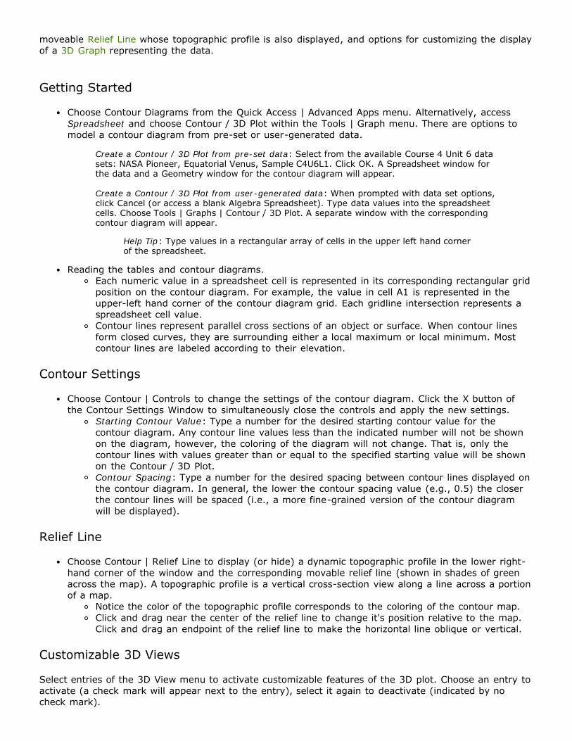
moveable Relief Line whose topographic profile is also displayed, and options for customizing the displayof a 3D Graph representing the data.

Getting Started

Choose Contour Diagrams from the Quick Access | Advanced Apps menu. Alternatively, accessSpreadsheet and choose Contour / 3D Plot within the Tools | Graph menu. There are options tomodel a contour diagram from pre-set or user-generated data.

Create a Contour / 3D Plot from pre-set data: Select from the available Course 4 Unit 6 datasets: NASA Pioneer, Equatorial Venus, Sample C4U6L1. Click OK. A Spreadsheet window forthe data and a Geometry window for the contour diagram will appear.

Create a Contour / 3D Plot from user-generated data: When prompted with data set options,click Cancel (or access a blank Algebra Spreadsheet). Type data values into the spreadsheetcells. Choose Tools | Graphs | Contour / 3D Plot. A separate window with the correspondingcontour diagram will appear.

Help Tip: Type values in a rectangular array of cells in the upper left hand cornerof the spreadsheet.

Reading the tables and contour diagrams.Each numeric value in a spreadsheet cell is represented in its corresponding rectangular gridposition on the contour diagram. For example, the value in cell A1 is represented in theupper-left hand corner of the contour diagram grid. Each gridline intersection represents aspreadsheet cell value.Contour lines represent parallel cross sections of an object or surface. When contour linesform closed curves, they are surrounding either a local maximum or local minimum. Mostcontour lines are labeled according to their elevation.

Contour Settings

Choose Contour | Controls to change the settings of the contour diagram. Click the X button ofthe Contour Settings Window to simultaneously close the controls and apply the new settings.

Starting Contour Value: Type a number for the desired starting contour value for thecontour diagram. Any contour line values less than the indicated number will not be shownon the diagram, however, the coloring of the diagram will not change. That is, only thecontour lines with values greater than or equal to the specified starting value will be shownon the Contour / 3D Plot.Contour Spacing: Type a number for the desired spacing between contour lines displayed onthe contour diagram. In general, the lower the contour spacing value (e.g., 0.5) the closerthe contour lines will be spaced (i.e., a more fine-grained version of the contour diagramwill be displayed).

Relief Line

Choose Contour | Relief Line to display (or hide) a dynamic topographic profile in the lower right-hand corner of the window and the corresponding movable relief line (shown in shades of greenacross the map). A topographic profile is a vertical cross-section view along a line across a portionof a map.

Notice the color of the topographic profile corresponds to the coloring of the contour map.Click and drag near the center of the relief line to change it's position relative to the map.Click and drag an endpoint of the relief line to make the horizontal line oblique or vertical.

Customizable 3D Views

Select entries of the 3D View menu to activate customizable features of the 3D plot. Choose an entry toactivate (a check mark will appear next to the entry), select it again to deactivate (indicated by nocheck mark).

Test 1 One observation beyond either Zone A. Test 2 Nine observations in a row on one halfof the chart.

Choose 3D View | On to turn on a 3D Plot of the corresponding contour diagram.Select 3D View | Contour to hide (or show) the contour map. When the contour diagram is hiddenand the 3D Plot is On, the 3D graph will appear larger in the viewing window with a x-y-z axisdisplayed.Select 3D View | Draw Grid /Mesh to show (or hide) the grid on the 3D model. Note the 3D Plotmust be On for this option to have an affect on the display.The Light Source option of the 3D View menu affects the brightness or dimness on the colorationon the 3D rendition of the map. Note the 3D Plot must be On for this option to have an affect onthe display.

Control Charts

Examine the run chart for a chosen data set, enter the desired mean and standarddeviation, then test for out-of-control behavior.

A run chart or control chart is a plot of data over time organized by a chosen mean and standarddeviation to provide a quick, visual check if a process has changed or gone out of control. Some of themethods or tests that industry uses to identify processes that have gone out of control are features ofthis custom app.

Recommended built-in data sets applicable to Control Chart include (but are not limited to): Los AngelesYearly Rainfall Averages, Apartment Temperatures, Manufactured Nails, and Gas Mileage. Alternatively,enter the desired data set into a Data Analysis data sheet, then access Control Chart from the CustomApps menu.

Instructions:

1. Type the desired Mean and Standard Deviation then press Enter. The mean will be marked at thevalue indicated, and Zones will be marked off by standard deviations on either side of the mean.The upper control limit (UCL) and lower control limit (LCL) are also indicated, each at threestandard deviations from the mean.

Help Tip 1: To read the chart, consider the placement of data points in relation to the Zonethey fall into. For instance, if a data point lies in Zone A, it is more than two, but less thanthree standard deviations from the mean.

Help Tip 2: The actual mean and standard deviation are not always the desired choices forsetting up a control chart. However, to obtain these values: (1) choose the button for BasicStatistics about the plotted data; or (2) use the Sample Mean and Std. Dev. entry of the Testsmenu.

2. Choose from the eight tests listed in the Tests menu to identify out-of-control behavior of thedata. NOTE: Each of the tests assumes that the individual values come from a normal distribution.

Help Tip: Make an informed decision about which test(s) to use by examining the data inrelation to the indicated Zones and the criteria listed for each test.

3. Depending on the test performed in Step 2, data points may be highlighted that match theidentified criteria of that particular test. Otherwise, nothing will be highlighted, indicating no out-of-control behavior.

Summary of Tests:

Test 3 Six observations in a row steadily increasingor decreasing.

Test 4 Fourteen observations in a rowalternating up or down.

Test 5 Two out of three observations in a row onone half of the chart and in Zone A orbeyond.

Test 6 Four out of five observations in a row onone half of the chart and in Zone B orbeyond.

Test 7 Fifteen observations in a row within the twoC zones.

Test 8 Eight observations in a row with none ineither Zone C.

Ranked-Choice Voting

Determine voting outcomes based on various ranked choice voting methods.

Instructions:

1. Start by selecting a table from the drop down menu.2. For pre-set tables, the categories and rankings will be displayed automatically. otherwise,

complete a blank table.3. Choose Vote Analysis to see the results.4. Select Details for a detailed analysis of each vote analysis method including: Plurality Method,

Majority Method, Runoff Method, Pairwise-Comparison Method, Points-For-Preferences Method, andInstant Runoff Voting (IRV) Method.

Weighted Voting

Investigate a voting situation with the Banzhaf Power Index; measure the weight of avoter and determine if their vote is critical or not.

Instructions:

1. Enter a quota.2. Enter the number of voters.3. Choose "Go" to assign voter weights to each voter (the number of voters was determined in Step

2).4. Analyze the results based on the assigned weights. A Banzhaf Power Index (BPI) is assigned for

each voter.

Vertex-Edge Graphs

A collection of vertices and edges, draw your own or create sample vertex-edge graphs.Add color, weight, and direction to a graph, run tests and algorithms, and investigate theadjacency matrix representation of a graph.

Vertex-Edge Graphs

A vertex-edge graph is a diagram consisting of a set of points (called vertices) along with segments orarcs (called edges) joining some or all of the points. The positions of the vertices, the lengths of theedges, and the shape of the graph are not essential. Important features of a graph include color,weight, direction, and how vertices are connected by edges.

Drawing Vertex-Edge Graphs

Draw Vertices or Edges : Select the button. Draw a vertex by clicking once in the sketcharea. To drawn an edge, hold down the mouse button as you click and drag from the center of avertex to a new location in the sketch area (or to an existing vertex), release the mouse button.Use these instructions as a guide for drawing a Simple Graph, Multigraph, Directed Graph,Weighted Graph, or Network.

Help Tip: Use the button to select, edit, move, and make stylistic changes to drawnvertices and edges.

Simple Graph: A simple graph is a graph that has at most one edge (i.e., either one edge or noedges) connecting any two vertices.Multigraph: A multigraph is characterized by vertices having more than one edge connecting them.

Help Tip: For two adjacent vertices (i.e., they are already connected by an edge) use the tool to add additional edges connecting them. When drawn, these edges will be slightly bent.

See also bending edges.

Directed Graph: A directed graph (or digraph) is a graph where the edges have a direction that isindicated by arrows.

Help Tip: Choose Options | Set Edge Type | Directed before drawing edges or after drawnedges have been Selected .

Weighted Graph: A weighted graph has positive numerical values assigned to its edges.

Help Tip: To assign weight to individual edges, chose the tool and double-click on a drawnedge. Type a positive numerical value into the text box then press Enter on the keyboard.

See also Weights.

Network: A network is a Directed graph with Weighted edges.

Pre-Constructed Graphs

Sample Graphs menu

This menu provides pre-constructed vertex-edge graph examples that are organized based on courseand by graph type. When a graph is chosen, it will be displayed in a separate window and may beedited and modified if desired.

Complete Graph: A complete graph is a connected graph that has exactly one edge between everypair of vertices. Choose Sample Graphs | Complete Graph to view an example of this type ofgraph. Type a positive integer for the number of vertices to display in the graph then click OK.Cycle: A cycle is a vertex-edge graph consisting of a single cycle - a route that uses each edgeand vertex exactly once and ends where it started. Choose Sample Graphs | Cycle to view anexample of this type of graph. Type a positive integer to specify the number of vertices then clickOK to display the graph.Complete Bipartite: A complete bipartite graph, denoted Kn,m, is a graph consisting of two sets of

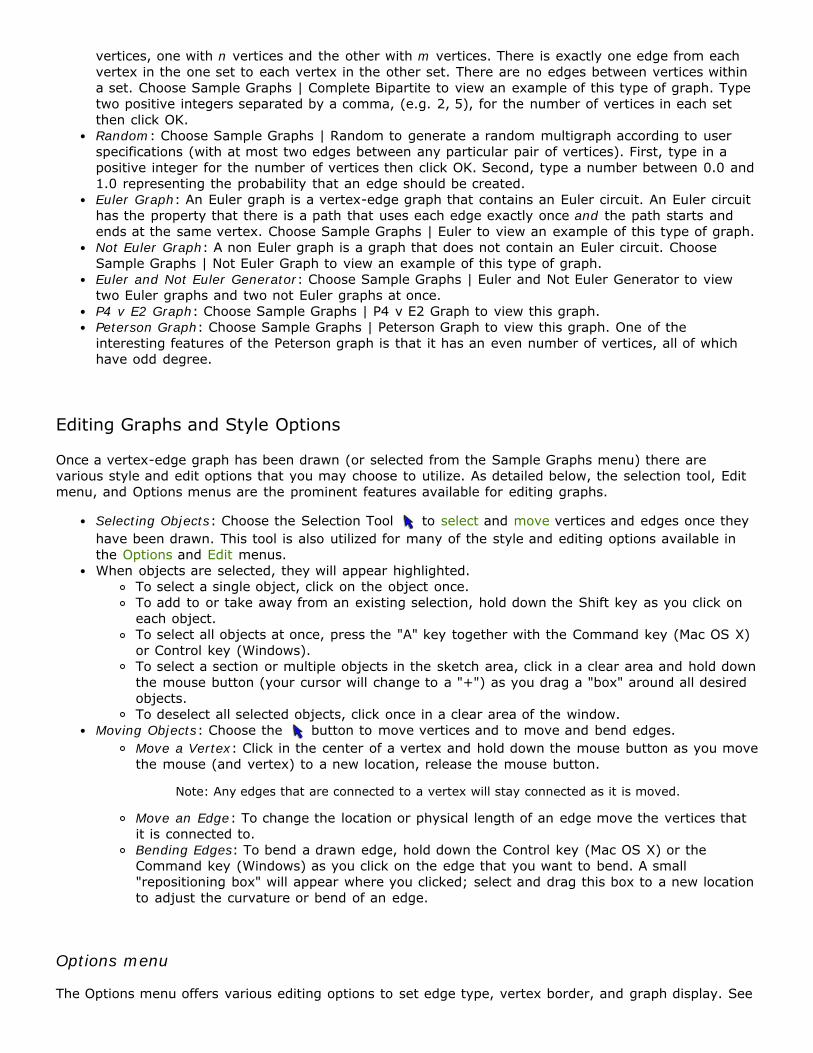
vertices, one with n vertices and the other with m vertices. There is exactly one edge from eachvertex in the one set to each vertex in the other set. There are no edges between vertices withina set. Choose Sample Graphs | Complete Bipartite to view an example of this type of graph. Typetwo positive integers separated by a comma, (e.g. 2, 5), for the number of vertices in each setthen click OK.Random: Choose Sample Graphs | Random to generate a random multigraph according to userspecifications (with at most two edges between any particular pair of vertices). First, type in apositive integer for the number of vertices then click OK. Second, type a number between 0.0 and1.0 representing the probability that an edge should be created.Euler Graph: An Euler graph is a vertex-edge graph that contains an Euler circuit. An Euler circuithas the property that there is a path that uses each edge exactly once and the path starts andends at the same vertex. Choose Sample Graphs | Euler to view an example of this type of graph.Not Euler Graph: A non Euler graph is a graph that does not contain an Euler circuit. ChooseSample Graphs | Not Euler Graph to view an example of this type of graph.Euler and Not Euler Generator: Choose Sample Graphs | Euler and Not Euler Generator to viewtwo Euler graphs and two not Euler graphs at once.P4 v E2 Graph: Choose Sample Graphs | P4 v E2 Graph to view this graph.Peterson Graph: Choose Sample Graphs | Peterson Graph to view this graph. One of theinteresting features of the Peterson graph is that it has an even number of vertices, all of whichhave odd degree.

Editing Graphs and Style Options

Once a vertex-edge graph has been drawn (or selected from the Sample Graphs menu) there arevarious style and edit options that you may choose to utilize. As detailed below, the selection tool, Editmenu, and Options menus are the prominent features available for editing graphs.

Selecting Objects: Choose the Selection Tool to select and move vertices and edges once theyhave been drawn. This tool is also utilized for many of the style and editing options available inthe Options and Edit menus.When objects are selected, they will appear highlighted.

To select a single object, click on the object once.To add to or take away from an existing selection, hold down the Shift key as you click oneach object.To select all objects at once, press the "A" key together with the Command key (Mac OS X)or Control key (Windows).To select a section or multiple objects in the sketch area, click in a clear area and hold downthe mouse button (your cursor will change to a "+") as you drag a "box" around all desiredobjects.To deselect all selected objects, click once in a clear area of the window.

Moving Objects: Choose the button to move vertices and to move and bend edges.Move a Vertex: Click in the center of a vertex and hold down the mouse button as you movethe mouse (and vertex) to a new location, release the mouse button.

Note: Any edges that are connected to a vertex will stay connected as it is moved.

Move an Edge: To change the location or physical length of an edge move the vertices thatit is connected to.Bending Edges: To bend a drawn edge, hold down the Control key (Mac OS X) or theCommand key (Windows) as you click on the edge that you want to bend. A small"repositioning box" will appear where you clicked; select and drag this box to a new locationto adjust the curvature or bend of an edge.

Options menu

The Options menu offers various editing options to set edge type, vertex border, and graph display. See

the Adjacency Matrix section for detailed help topics related to adjacency matrices.

Add Loop to Vertices(s): A loop is an edge that connects a vertex to itself. Select a vertex (ormultiple vertices) then choose Options | Add Loop to Vertice(s).Set Edge Type: Use the Options | Set Edge Type entry to set the edge type of drawn edges to beeither Undirected or Directed.

Undirected: Undirected edges do not indicate direction between vertices. In other words, theedges do not have arrows on them. This is the default graph style.Directed: Directed edges have arrows indicating direction from one vertex to another.Choose Options | Set Edge Type | Directed, then all edges drawn after this selection will bedirected. Alternatively, Select undirected edges that have already been drawn, thenchoose Set Edge Type | Directed to show the direction on these edges. The direction isdetermined based on how the graph is drawn.

Help Tip: To remove direction from drawn edges Select them and chooseOptions | Set Edge | Undirected.

Set Vertex Border: Use the Set Vertex Border entry of the Options menu to set the type of borderused for vertices.

Circles: Choose Options | Set Vertex Border | Circles to specify the shape of selected drawnvertices to be circular. This is the default setting that will be automatically applied to all newdrawings.

Rectangles: Choose Options | Set Vertex Border | Rectangles to specify the shape ofselected drawn vertices to be rectangular.

Set Graph Display: Use Options | Set Graph Display entry to toggle the weight, color, and degreesettings for vertices and edges.

Weights: Weights are positive numerical values assigned to edges. Choose Options | SetGraph Display | Weights to show (or hide) any user specified or pre-constructed weights. Acheckmark next to this entry indicates that any user specified or pre-constructed weightswill be shown - this is the default setting.Name/Add Weight : Choose the button then double-click an edge, type text (to name)or numbers (to weight) into the text box, then press Enter.

Help Tip: Add weight to drawn vertices by separating any text and weight with acomma. For example, type Theme, 2 then press Enter. This will be useful for creatingyour own digraphs to be used with the Critical Path Algorithm.

Colors: Choose Options | Set Graph Display | Colors to show (or hide) any user specifiedcolors on a graph. A checkmark next to this entry indicates that any user specified colorswill be shown - this is the default setting.Color Vertices or Edges : To change the color of a vertex or edge to create a coloredgraph, follow these steps: (1) Select the object(s) you wish to color. (2) Choose the button to view all color options. (3) Click on the desired color then click OK to color allselected objects that color. Alternatively, perform Steps 2-3 then Step 1.Degrees: Choose Set Graph Display | Degrees in the Options menu to view (or hide) thedegree of all vertices on a given graph. At least one vertex must be drawn before choosingthis option.Degree of a Vertex: The degree of a vertex is the number of edges touching a vertex. If anedge loops back to the same vertex, that counts as two edge-touchings.

Edit menu

The Edit menu offers stylistic options for existing graphs. Most menu options are also available astoolbar buttons.

Choose Edit | Undo to reverse the most recent action that you performed. Subsequentexecution of this option will continue to reverse previous actions.

Note: Not all actions can be reversed using the undo feature (e.g., the coloring of vertices oredges).

Choose Edit | Redo to reverse the action of the Undo button.Select an object or objects that you would like to remove. Choose Edit | Cut or the buttonto remove the selected object(s).Choose Edit | Duplicate Graph to produce an exact copy of the currently selected graph.Choose Edit | Tile All Windows or the button to view all open windows at once.

Note: You cannot use the Undo option to reverse this action, instead you must resize or usethe Scaling Graphs feature as described below.

Scaling Graphs: To resize or scale a window, use the drop-down menu in the bottom, right-hand corner and select a scale size. Available percentage options are: 25, 50, 75, 100, 200,300, other.

Help Tip: The more windows that are open at one time, the smaller they will each bescaled down when tiled, thus the graphs on each window may be harder to see. It maybe helpful to only view four graphs at a time in this way.

Alternative Graph Viewing Option: When more than one window is open at a time, selectwhich one you would like to view by using the drop-down menu at the bottom-middle of theVertex-Edge Graph window. This drop down list contains the names of all open windows.

Help Tip: The default window name is "Untitled," but this changes to the file name youchoose upon Saving.

File Options

The File menu offers options to open, save, and print new and existing work.

See Save & Print for help on Save, Print, and Open options.

New versus Clear All: Choose File | New to create a separate blank window. Alternatively, choosethe Clear All button to erase all drawn objects in the active window, without saving.

Note: Choosing File | New will not replace or clear any previously drawn graphs in otherwindows.

Close Window: Choose File | Close to close the active window without saving. Alternatively, youmay use the close button (an "X") on the title bar of an individual window to close it.Close All Windows: Choose File | Close All to close all windows within Vertex-Edge Graph withoutsaving.Choose File | Exit to quit the tools. Contents of any open windows will be lost unless Saved first

Help Tip 1: To exit the Vertex-Edge Graph tool without quitting the tools use the close buttonX.

Help Tip 2: To close individual windows within Vertex-Edge Graph, choose Close or Close All inthe File menu (or use the close button X on each individual window).

Adjacency Matrix

An adjacency matrix is a matrix representation of a vertex-edge graph in which each entry of the matrixindicates whether the corresponding pair of vertices are connected by any edges (or rather, areadjacent). Each entry of the matrix represents the number of directed edges connecting the row vertexto the column vertex. A zero (0) indicates that the vertices are not adjacent.

Display the Adjacency Matrix: Select Options | Adjacency Matrix to show the adjacency matrix forthe drawn graph in a separate window. Click on the cells of this matrix to highlight thecorresponding edge(s) on the graph.Choose Options | Power of Adjacency Matrix to calculate a specified power of the adjacency matrix

for the drawn graph. A message window will prompt you to enter the desired power that you wishto compute, type a positive integer then click OK to view the matrix in a separate window. Clickon the cells of this matrix to highlight the corresponding edge(s) on the graph.Choose Options | Distance Matrix to view the distance matrix for a Weighted graph. Each cell ofthe matrix represents the distance between the column vertex and row vertex. Click on the cellsof this matrix to highlight the corresponding edge(s) on the graph.Choose Options | Paths of Length n Matrix to display a matrix that shows the number of possiblepaths of length n that go from the row vertex to the column vertex. Before you are able to viewthe matrix, a message window will prompt you to enter the desired path length; enter a positiveinteger value then click OK. Click on the cells of this matrix to highlight the specified path on thegraph or to view all possible paths of length n (click on an entry of this list to highlight the pathon the graph).Choose Options | Adj Matrix to CAS to show the adjacency matrix for the drawn graph in the CASHome and Y= tabs.

Tests & Algorithms

Tests menu

To test a drawn graph or network, choose an option from the Tests menu. A separate message box willdisplay the result of the test. If the test was successful, the message box will list the appropriatevertices used for the chosen test.

Connected: Choose Tests | Connected to determine if the drawn graph is connected. A connectedgraph is a graph that is all in one piece. That is, from each vertex there is at least one path toevery other vertex. If a graph is not connected, the message box will specify how many connectedcomponents make up the graph. Additionally, users can click on the drop-down bar to highlight anindividual unconnected component.Bipartite: Choose Tests | Bipartite to determine if the drawn graph is bipartite. A bipartite graphhas the property that the vertices can be partitioned into two sets such that every edge connectsone vertex from each set. If a graph is bipartite, separate bipartite sets will be highlighted.Additionally, users can choose to display the graph with the bipartite sets separated.Euler: Choose Tests | Euler to determine if an Euler circuit exists for the graph. An Euler circuithas the property that there is a path that uses each edge exactly once and the path starts andends at the same vertex.

Help Tip: The Euler test will only display whether or not the graph contains an Euler circuit, itwill not tell you what the Euler circuit is. Use the Euler Circuit Algorithm to display what theEuler circuit is.

Algorithms menu

The Algorithms menu offers several different types of algorithms that can be used after a graph ornetwork is drawn. An algorithm is a list of step-by-step instructions or a systematic step-by-stepprocedure. General instructions for how to run an algorithm are provided below, followed by a list ofpossible algorithms.

How to Run an Algorithm For a Drawn Graph:

1. Choose Automatic or Step Through in the Algorithms menu to determine the way the algorithmwill be completed. A check mark will appear next to the selected option.

Automatic: Choose Automatic in the Algorithms menu to automatically carry out and displaythe final result of the algorithm.

Important Note: The displayed result of an algorithm may or may not be the onlypossible result.

Step Through: Choose Step Through in the Algorithms menu for the chosen algorithm to beimplemented step-by-step with user interaction.

Important Note: Messages with instructions may be displayed in the lower-left handcorner of the screen, or in separate message windows.

2. Select any of the available algorithms that are listed in the Algorithms menu to perform thatalgorithm on the drawn graph.

Important Note: Be sure that only one type of procedure and algorithm are selected at once;uncheck any unwanted options by clicking on them.

3. The chosen algorithm will run as Automatic or Step Through (depending on the choice made inStep 1). See below for algorithm-specific help topics.

Algorithms

Minimum Hamilton Circuit: A Hamilton Circuit is a route through a graph that starts at one vertex,visits all the others vertices exactly once, and finishes where it started. The purpose of thisalgorithm is to find the shortest route (minimum total weight) that meets the criterion of being aHamilton Circuit.

Automatic: The algorithm will automatically highlight the minimum Hamilton Circuit on agraph. If there are two equivalent minimum circuits, a new message window will appearwith a drop down menu that will allow you to show each highlighted circuit individually.

List Hamilton Circuits: A Hamilton Circuit is a path that begins and ends at the same vertex andthat visits each vertex of the graph exactly once. The purpose of this option is to list all possibleHamilton Circuits of a particular graph. If available, Hamilton Circuits will be organized in aninteractive table by weight. Click in the table to highlight a listed circuit on the graph. This optionwill run the same and produce the same results regardless of whether the Automatic or StepThrough option is chosen.Nearest Neighbor: One purpose to using the Nearest Neighbor algorithm is to find a minimumspanning tree, however, this algorithm is not a guaranteed method for finding a minimumspanning tree. In the Nearest Neighbor algorithm, choose a vertex to start at, and successivelyadd shortest edges without creating circuits, but only add edges that are connected to the vertexwhere you are at each step.

Automatic: The algorithm will automatically highlight a route through the drawn graph andshow the result of performing the algorithm in a window. Messages will prompt you toconsider whether every vertex has been reached and whether the total weight is minimum.Each iteration of this automatic algorithm may produce a different result, that may or maynot produce a minimum spanning tree.Step Through: You will first be prompted to click on a starting vertex on the drawn graph,then select a valid minimum edge. Recall that you must choose edges that are connected(adjacent) to the vertex that you chose. When there are no more edges to be selected, theedge choices and total weight will be displayed in a window. Messages will prompt you toconsider whether every vertex has been reached and whether the total weight is minimum.Try starting at different vertices each time you complete this step through algorithm to seewhat results.

Kruskal's Minimum Spanning Tree: In Kruskal's "best-edge" algorithm, you successively addshortest edges (of least weight) without creating circuits, and any edge you add does not have tobe connected to a previously added edge. This algorithm is guaranteed to produce a minimumspanning tree. Note that different runs of Kruskal's algorithm on the same graph could producedifferent spanning trees.

Automatic: The algorithm will automatically highlight a route through the drawn graph andshow the total weight of the highlighted edges in a window. Recall that this may not be theonly minimum spanning tree for a particular graph.Step Through: Prompts in a message window will instruct you to first select the edge withthe least weight by clicking on it on the graph. You will then continue in this manner,choosing the next "valid" edges (as described above). When the chosen edges span thegraph (without creating a circuit), the total weight of the selected edges will be displayed.

Prim's Minimum Spanning Tree: In Prim's algorithm, you start at a vertex and successively addshortest edges without creating circuits, and any edge you add must be connected to any vertexalready reached. This algorithm is guaranteed to produce a minimum spanning tree. Note thatdifferent runs of Prim's algorithm on the same graph could produce different spanning trees.

Automatic: The algorithm will highlight a possible route on the drawn graph and display thetotal weight and order of chosen vertices in a message window. Recall that the shown routemay not be the only minimum spanning tree for a particular graph.Step Through: A message window will prompt you to choose a starting vertex by clicking onit on the graph. You will then be prompted to click on "valid" edges (as described above). Ifyou choose an "invalid" edge, check the rules of the algorithm and try again. When thechosen edges span the graph (without creating a circuit), the total weight of the selectededges will be displayed.

List Spanning Trees: A spanning tree is a tree in a connected graph that reaches (i.e. includes orconnects) all the vertices in the graph. Note that a connected graph that has no circuits is called atree. The purpose of this option is to list all possible spanning trees of a particular graph. Allpossible spanning trees will be listed in an interactive table that lists the edges used (given byvertices; e.g., {A,B} is the edge connecting vertices A and B). Click on a spanning tree tohighlight its path on the graph. This option will run the same and produce the same resultsregardless of whether the Automatic or Step Through option is chosen.Shortest Path: The purpose of this algorithm is to determine the shortest path between twovertices. First Select two vertices (and no edges), then choose Shortest Path in the Algorithmsmenu, a message will display the shortest path as an integer value representing the fewestnumber of edges required to get from one vertex to another. The weight of this shortest path willbe displayed once you click OK on the first prompt window. This option will run the same andproduce the same results regardless of whether the Automatic or Step Through option is chosen.Critical Path: A path through a Directed graph (digraph) that corresponds to the earliest finishtime is called a Critical Path. Note that it is the length of the longest path that gives the earliestfinish time. A good sample graph to use for this algorithm is the Feasibility Study Digraph, foundin the Unit 6 Network Optimization option of the Sample Graphs menu. Otherwise, create yourown digraph with weighted vertices by separating the text and weight with a comma.

Automatic: The algorithm will automatically display the critical path and the total weight ofthe critical path in a message window. Also notice that the path will be highlighted on thedrawn graph.

Circuit Finder: A circuit is a path which begins and ends at the same vertex. Note that a circuitdoes not necessarily have to make use of every vertex or edge, nor is a circuit restricted to usingany particular vertex only once.

Automatic: The algorithm will color the edges of each (partial) circuit found. The user canthen choose to view a partial circuit from the drop-down list in the message box.Step Through: All edges will initially appear gray in color. Users can click on any edge toshow the associated partial circuit by coloring all appropriate edges.

Euler Circuit: If it is possible to start at a vertex and pass along each edge without going over anyof them more than once, then the graph has an Euler path. If the path ends at the same vertex atwhich you started, then it is called an Euler circuit.

Automatic: The algorithm will automatically color partial circuits in different colors, both onthe graph and in a window with a colored list of vertices. Additionally, an Euler circuit isthen traced out by stitching together the colored partial circuits.Step Through: The algorithm will display the partial circuits in different colors on the graphand in a separate window with a colored list of vertices. In another series of windows, clickOK to see how all colored partial circuits are stitched together as an Euler circuit is tracedout sequentially.

Welsh-Powell: The purpose of this algorithm is to color each vertex starting with a vertex havingthe highest degree. You then select another vertex of highest degree that is not connected to theprevious vertex. You continue doing this until you are required to switch colors, and then theprocess starts over again.

Automatic: The algorithm will automatically color the vertices on the graph and display awindow describing the minimum number of colors used and the order in which they werechosen.Step Through: In the bottom-left corner of the main window, a message will prompt you toselect the next vertex. Select the appropriate vertices in order according to the algorithm.The program will notify you when a new color is needed for the coloring. The minimumnumber of colors and an order will be displayed in a separate window when complete.

Help Tip: Choose Options | Degrees before using this algorithm.

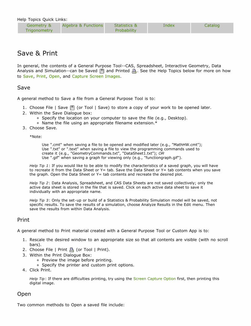
Help Topics Quick Links: Geometry &Trigonometry

Algebra & Functions Statistics &Probability

Index Catalog

Save & Print

In general, the contents of a General Purpose Tool--CAS, Spreadsheet, Interactive Geometry, DataAnalysis and Simulation--can be Saved and Printed . See the Help Topics below for more on howto Save, Print, Open, and Capture Screen Images.

Save

A general method to Save a file from a General Purpose Tool is to:

1. Choose File | Save (or Tool | Save) to store a copy of your work to be opened later.2. Within the Save Dialogue box:

Specify the location on your computer to save the file (e.g., Desktop).Name the file using an appropriate filename extension.*

3. Choose Save.

*Note:

Use ".cmt" when saving a file to be opened and modified later (e.g., "MathHW.cmt");Use ".txt" or ".text" when saving a file to view the programming commands used tocreate it (e.g., "GeometryCommands.txt", "DataSheet1.txt"); OR Use ".gif" when saving a graph for viewing only (e.g., "functiongraph.gif").

Help Tip 1: If you would like to be able to modify the characteristics of a saved graph, you will haveto recreate it from the Data Sheet or Y= tab. Save the Data Sheet or Y= tab contents when you savethe graph. Open the Data Sheet or Y= tab contents and recreate the desired plot.

Help Tip 2: Data Analysis, Spreadsheet, and CAS Data Sheets are not saved collectively; only theactive data sheet is stored in the file that is saved. Click on each active data sheet to save itindividually with an appropriate name.

Help Tip 3: Only the set-up or build of a Statistics & Probability Simulation model will be saved, notspecific results. To save the results of a simulation, choose Analyze Results in the Edit menu. Thensave the results from within Data Analysis.

Print

A general method to Print material created with a General Purpose Tool or Custom App is to:

1. Rescale the desired window to an appropriate size so that all contents are visible (with no scrollbars).

2. Choose File | Print (or Tool | Print).3. Within the Print Dialogue Box:

Preview the image before printing.Specify the printer and custom print options.

4. Click Print.

Help Tip: If there are difficulties printing, try using the Screen Capture Option first, then printing thisdigital image.

Open

Two common methods to Open a saved file include:

Go to the desired General Purpose Tool and choose File | Open . Locate the file on yourcomputer and choose Open. ORLocate the file on your computer and double-click it.

Double-click a saved CMT file to automatically open it within Core Math Tools.Double-click a saved TEXT file to automatically open it within your computer's text editor(e.g., WordPad, TextEdit).Double-click a saved GIF file to automatically open it within your computer's image viewer(e.g., Adobe, Preview).

Help Tip 1: Double-clicking a saved .txt file will open it in the default text editor program on yourcomputer. From the text editor program you may manually change the commands (for a geometryfile) or the data sheet name and column headers (for a spreadsheet file). Additionally, you may opendata sheet files from within other spreadsheet programs (e.g., Microsoft Excel).

Help Tip 2: A saved image file (such as a graph with file name extension .gif) will be opened with thedefault picture viewer program on your computer (e.g., Picture Viewer in Windows or Preview in MacOS X).

Screen Capture (Digital Image)

Capture a Screen Image of your work to embed as a digital file within another application, or to print.Two options are given below (the first might not be available from all tools, while the second can beapplied at any time).

Choose File | Copy to Clipboard. Open an application such as Word, TextEdit, or Paint. ChooseEdit | Paste (Command+V). The tool image will be inserted as a digital image in this otherapplication. Save, Print, and modify as desired.Use the screen capture feature of your computer:

Windows--press the "PrtSc" key. Follow an analogous process as the "Copy to Clipboard"option (above).Mac--simultaenously press the keys "Command+Shift+3" or "Command+Shift+4+Space". Animage file will automatically be saved to your computer.

Quick Links:Statistics &Probability

Data Analysis Algebra & Functions Spreadsheet CAS

Data Sets

Data sets can be accessed through the Data menu of Data Analysis, the File | Data menu ofSpreadsheet, and the File | Data menu of CAS. Click on the name of a Data Set below to automaticallydownload this file and open it within Data Analysis of Core Math Tools (an Internet connection isrequired for file download).

Data Analysis | Data Spreadsheet | Data CAS | File | Data

Univariate DataCategorical Data2000 State Motorcycle Statistics

Chicago White Sox

Quantitative Data2000 State Motorcycle StatisticsAchievement Test ScoresApartment TemperaturesBest ActressCertificate PerimetersConcord and Portland PrecipitationDissolution TimesFastest Growing FranchisesGas MileageHeights of Young AdultsJanuary SunshineLand UseLos Angeles Rainfall

Manufactured NailsMean Hourly EarningsMin and Max TemperaturesNickel WeightsNon-normal DistributionNumber of MarriagesNumber of Video GamesPSU Women's HeightsRatings of Movie ShowingsStudy TimeSunshine for All MonthsU.S. Census 2000 & 2010Vertical Jumps

Bivariate DataCategorical DataArtificial TurfBicycle HelmetCryingFashionHispanic OriginsIBS and Anxiety

LaptopsOfficer TraineesSeasonsTV RolesVirginia Crashes

Data Analysis | Data Spreadsheet | Data CAS | File | Data

Bivariate DataQuantitative Data100-meter FreestyleAIDS Fatalities in the U.S.

Los Angeles Flight Alt. and Temp.Major U.S. City Populations

All Manatee MortalitiesAltitude/Atmospheric PressureAnimal Brain and Body WeightsBaby Boys WalkingBacteria Growth IBacteria Growth IIBaseball AveragesBlood Lead LevelsBraking Road TestCaninesCar Skid MarksChicago White SoxCold SurgeryCompact CarsCrawling AgeCricket ChirpsCumulative AIDS DeathsDow Jones AveragesDSM Monthly TempsFederal Minimum WageFertilizing CostFlights to/from ChicagoFree Fall SpeedHamburger Nutrition IHamburger Nutrition IIHamburger Nutrition IIIHealth and NutritionHipposHorse StrideInstructor AttributesLeg and Stride LengthLight Intensity

Manatee Watercraft MortalitiesMarriage/Divorce RatesMedian IncomeMen’s 100-meter RunMozart/SilenceNon-linear (x,y) Values INon-linear (x,y) Values IINon-linear (x,y) Values IIIPeak Cherry Tree BloomingPenny StackingPlanet Orbits (km)Planet Orbits (mi)Plant GrowthRadioactive IsotopeRadioactive Waste ExposureRamp Height and TimeRamp Time and DistanceRiverdale Adventure ClubSatellite RadioSeal SizesSelected Fast FoodSmell TestSphere Radius and Surface AreaSphere Surface Area and VolumeSurgery Time and CostTaking ChancesTree AgeU.S. CensusU.S. Public DebtVoters in U.S. ElectionsWomen’s 100-meter RunWorld Population

Spreadsheet | Data

Multivariate DataQuantitative DataEquatorial VenusMars

NASA PioneerTerrain Elevations

Help Topics Quick Links: At a Glance Geometry &

TrigonometryAlgebra & Functions Statistics &

ProbabilityIndex

Catalog

The Catalog is cumulative across the entire suite of tools.

A B C D E F G H I J K L M N O P Q R S T U V W X Y Z Symbols

Strand-specific Indices and Catalogs are available for the general purpose tools:

Algebra & Functions: Commands, Index, CAS, SpreadsheetGeometry & Trigonometry: Commands, Index, Interactive GeometryStatistics & Probability: Commands, Index, Data Analysis, Simulation

Aabs()[abs number] ans(1) angleaverage() Bbinomcdf()binompdf()bisectCceil()chisqcdf()chisqpdf()circleclearcol()comb()complex()conj()cos()[cos number] count() csDder()det()drawEexp()expand()Ffact()factor()Fcdf()Fpdf()floor()[function expression]Hhalfplane

Iiid()imag()infoinput "Prompt" variable int()intersectioninv()invcos()[invcos number] invNorm()invsin()[invsin number] invT()invtan()[invtan number] Lletlineln()log()Mmatrix()max()midpointNnormalcdf()normalpdf()Pparallelpath pointperpendicularperm()piecewise()pointpolygonprod()programRrayreal()

Sscalesegmentshowsimplify()sin()[sin number] size()solve()sqr()sqrt()[sqrt number]stdev() sum()Ttan()[tan number] tangentstcdf()tpdf()tr()translateVvectorvisibleSymbols+ (add)@ (at)/(divide)= (equal to)> (greater than)>= (greater than or equal to)< (less than)<= (less than or equal to)% (modulo)* (multiply)!= (not equal to)^ (raise to the power of)- (subtract)

reflectregeq()root()rotaterow()

Help Topics Quick Links: At a Glance Geometry &

TrigonometryAlgebra & Functions Statistics &

ProbabilityCatalog

Cumulative Index of Help Topics

All help topics that are available for Core Math Tools are listed below in alphabetical order.

Strand-specific Indices and Catalogs are also available for the general purpose tools:

Algebra & Functions: Commands, Index, CAS, SpreadsheetGeometry & Trigonometry: Commands, Index, Interactive GeometryStatistics & Probability: Commands, Index, Data Analysis, Simulation

2D Functions3D Plots, Bounds3D Plot Option (CAS)3D Plot (Spreadsheet) abs() [abs number]Add OutcomeAdd VectorsAdjacency MatrixAdvanced Apps Algebra & Functions CommandsAlignment AnalysisAnalyze ResultsAngle, angleAngle MeasureAngle BisectorAnimationAreaans(1) ApproximateAuto NumericAuto ScaleAuto Simplifyaverage()Basic Statistics (Simulation)Basic Statistics Functionsbinomcdf()Binomial Distributionsbinompdf() bisectBox PlotBuild SimulationCalculate, CalculationCASceil()

CellCell ReferenceCenter AlignChange Style of SelectedChi-Square Testchisqcdf()chisqpdf() Circle, circleCircumferenceclearClear All (Y=) col()Column FormulaColumn Name comb() Combinatorics Functions Command Line (CAS)Command Window (Geometry)Commands (Algebra)Commands (Geometry)Common Eventscomplex() Complex NumbersComputationsConduct Simulationsconj() ConstructionsContour (3D Plot)Contour DiagramsCoordinatesCoordinate GeometryCopy cos() [cos number] count()cs

Custom Apps (Algebra &Functions)Custom Apps (Geometry)Custom Apps (Statistics &Probability)Custom EventsCutData (CAS)Data (Data Analysis)Data (Spreadsheet)Data AnalysisData Sets Data SheetDefault SettingsDefault StylesDefine EquationDegree Mode (CAS)Degree Mode (Spreadsheet)Delete EquationDelete OutcomeDelete Row, Delete ColumnsDelete SelectedDelta Xder() Descriptive StatisticsDeselect AllDesign by Robotdet()Directed Vertex Edge GraphDistribution EventsDistribution of SampleDraw, drawDraw AxesDraw GridDraw MeansDraw Moveable Model

Draw Regression ModelDraw ResidualsDraw SquaresEdit Cells Edit Equation

Home tabi id()imag()Implicit

Models menuMove and Shift CellsNNew (Simulation)New Matrix

Edit FormulaEdit menuEdit Styles and Settings (DataAnalysis)EnableEnter/Edit a ModelError ThermometerEstimate CenterEstimate Center and SpreadExamples (Spreadsheet)Excludedexp()expand() Explore Angles and ArcsExplore RadiansExplore Similar TrianglesExplore SSAfact()FastFastestFcdf()Fpdf()Figure or polygonFill DownFill ColorFilledFixed Cell Referencefloor()FontFormulasFrequency Table Graph[function expression]Function IterationGoodness of FitGraph (CAS)Graph (Simulation)Graph (Spreadsheet) Graphical DisplaysGraph menu (Data Analysis) GridGrid StyleGuess CorrelationHalf Plane, halfplaneHide CoordinatesHide SelectedHide SurfacesHistogram

infoinput "Prompt" variableInsert CellsInsert Functionint() Intersection, intersectioninv()invcos()[invcos number]invNorm()invsin()[invsin number]invT() invtan()[invtan number]Labels (Geometry)Labels (Histogram)Left AlignLengthsletLine, lineLinear Programming List of Shapesln() log() Make Equally LikelyMath ToolbarMatricesmatrix()Matrix EditorMatrix FunctionsMatrix ExampleMatrix Plotmax()MaximumMaximum X, YMeanMeasureMedianMediumMeta EventsMidpoint, midpointMinimum Minimum X, YMode (CAS)Mode (Spreadsheet)Modeling

Normal Plotnormalcdf()normalpdf() Options menu (Geometry)Options menu (Graph) Options menu (Home)Options menu (Settings)Other Functions Parallel, parallelParameter Parametric Plot OptionPastepath pointPerimeterperm() Perpendicular, perpendicularpiecewise() Plot Information (Data Analysis)Plot Style Point, pointPolar Plot Option Polygon, polygonPrintprod() programProgrammingQ1Q3Radian Mode (CAS)Radian Mode (Spreadsheet)Random BinomialRandom NormalRandomization DistributionRay, rayreal()Reflect, reflectregeq() RegressionRectangular Plot OptionRegression Relative Frequencies (Simulation)ResetRight Alignroot() Rotate, rotaterow()Run Simulation

Sample MatrixSample SimulationSample Standard DeviationSample VarianceSaveScale, scaleScatterplot (CAS)Scatterplot (Data Analysis)Segment, segmentSelectSelect Equation Set # of Digits (CAS)

StepStopStyle Windowsqr() sqrt() [sqrt number]stdev()sum() Summary Statistics (CAS)Summary Statistics (Spreadsheet)Surface of RevolutionSymbolic Manipulation

Set # of Digits (Spreadsheet) Set # of Digits (Data Analysis)SettingsSettings (Home)Settings (Y=) ShadingShift Cells showShow CoordinatesShow Critical ValuesShow Equation (CAS)Show Equations (Data Analysis)Show Expected CountsShow Expected PercentsShow HiddenShow Predicted Value(s)Simple Eventssimplify() SimulationSimultaneoussin()[sin number]size()Slice 3D Plot Slice X, Y, Z Slicing a Double ConeSlicing or Unfolding PolyhedraSliders, Snap to MarkSlopesSlowSnap to Grid solve() Sort SpeedSplit View with TableSpreadsheet StackedStandard WindowStartStatistical Analysis

Syntax ErrorSynthetic GeometryTable (CAS)Table of Results (Simulation)tan()[tan number]Tangents, tangentstcdf()Test for IndependenceTest for HomogeneityThicknessTiledTilings with Regular PolygonsTilings with Triangles orQuadrilateralsTime Series tpdf() tr()TransformationsTranslate, translateTriangle Congruence Trig WindowTrigonometric FunctionsUndirected Vertex Edge GraphUndo (Geometry)Undo (Simulation)Vector, vectorView Matrix AsView menu (Simulation)View Options (Graph)View Results (Simulation)Visible, visibleWindow Scale Y=Zoom BoxZoom InZoom OutZoom SettingsZoom SqrZoom StdZoom Trig

License, Permissions, and Copyright Information

Core Math Tools is a suite of Algebra & Functions, Geometry & Trigonometry, andStatistics & Probability software tools designed to support implementation of theCommon Core State Standards for Mathematics.© 2012 B. A. Keller, Michigan State University and the Core-Plus Mathematics Project, Western MichiganUniversity.

This material is based on work supported by the National Science Foundation (NSF) under Grant No. ESI-0137718, Grant No. DRL-1020312, and Grant No. DRL-1201917. Opinions expressed are those of theauthors and do not necessarily reflect the views of the NSF.

Suite is built using the following resources:© 2006-11, CPMP-Tools, Core-Plus Mathematics Project, www.wmich.edu/cpmp/CPMP-Tools© 2000, Sun Microsystems Inc. Icons, www.sun.com© 2002, Calico, Charles Stanton, www.math.csub.edu/staton/calico© 2002, Colt/Cern, dsd.lbl.gov/~hoschek/colt© 2002, HotEq, www.esr.ruhr-uni-bochum.de/VCLab/software/HotEqn/HotEqn.html© 2007 (2010), JavaView, www.javaview.de © 2003, Jeks, www.eteks.com© 2005, JGraph, www.jgraph.com© 2010, Bortolossi, Humberto, www.uff.br/cdme/pdp/pdp-html/pdp-en.html

These resources are used with permission for Core Math Tools. Each resource has its own copyright,licensing and use requirements, and you should see the corresponding website.

3D Graphical library (including the pre-build and fully functional algorithms to cut, unfold, truncate, punchand stellate polyhedra): JavaView - Interactive 3D Geometry and Visualization.

3D Custom Apps: www.javaview.de/demo/PaRotation.htmlwww.fmi.uni-sofia.bg/projects/daad/smbconf_en_nojs/javaview/beograd.htmlPlethora of Polyhedra, www.uff.br/cdme/pdp/pdp-html/pdp-en.html

Core Math Tools is free; you can use it and redistribute it under the terms of the GNU General PublicLicense as published by the Free Software Foundation; either version 2 of the License, or any later version.

The software is distributed in the hope that it will be broadly useful to the field, but WITHOUT ANYWARRANTY; without even the implied warranty of MERCHANTABILITY or FITNESS FOR A PARTICULARPURPOSE. See the GNU General Public License for more details.

You should have received a copy of the GNU General Public License along with this program; if not, write tothe Free Software Foundation, Inc., 51 Franklin St, Fifth Floor, Boston, MA 02110-1301 USA

GNU GENERAL PUBLIC LICENSE Version 2, June 1991

Copyright (C) 1989, 1991 Free Software Foundation, Inc. 51 Franklin St, Fifth Floor, Boston, MA 02110-1301 USA Everyone is permitted to copy and distribute verbatim copies of this license document, but changing it is not allowed.

Preamble

The licenses for most software are designed to take away yourfreedom to share and change it. By contrast, the GNU General PublicLicense is intended to guarantee your freedom to share and change freesoftware--to make sure the software is free for all its users. ThisGeneral Public License applies to most of the Free SoftwareFoundation's software and to any other program whose authors commit tousing it. (Some other Free Software Foundation software is covered bythe GNU Library General Public License instead.) You can apply it toyour programs, too.

When we speak of free software, we are referring to freedom, notprice. Our General Public Licenses are designed to make sure that youhave the freedom to distribute copies of free software (and charge forthis service if you wish), that you receive source code or can get itif you want it, that you can change the software or use pieces of itin new free programs; and that you know you can do these things.

To protect your rights, we need to make restrictions that forbidanyone to deny you these rights or to ask you to surrender the rights.These restrictions translate to certain responsibilities for you if youdistribute copies of the software, or if you modify it.

For example, if you distribute copies of such a program, whethergratis or for a fee, you must give the recipients all the rights thatyou have. You must make sure that they, too, receive or can get thesource code. And you must show them these terms so they know theirrights.

We protect your rights with two steps: (1) copyright the software, and(2) offer you this license which gives you legal permission to copy,distribute and/or modify the software.

Also, for each author's protection and ours, we want to make certainthat everyone understands that there is no warranty for this freesoftware. If the software is modified by someone else and passed on, wewant its recipients to know that what they have is not the original, sothat any problems introduced by others will not reflect on the originalauthors' reputations.

Finally, any free program is threatened constantly by softwarepatents. We wish to avoid the danger that redistributors of a freeprogram will individually obtain patent licenses, in effect making the

program proprietary. To prevent this, we have made it clear that anypatent must be licensed for everyone's free use or not licensed at all.

The precise terms and conditions for copying, distribution andmodification follow.

GNU GENERAL PUBLIC LICENSE TERMS AND CONDITIONS FOR COPYING, DISTRIBUTION AND MODIFICATION

0. This License applies to any program or other work which containsa notice placed by the copyright holder saying it may be distributedunder the terms of this General Public License. The "Program", below,refers to any such program or work, and a "work based on the Program"means either the Program or any derivative work under copyright law:that is to say, a work containing the Program or a portion of it,either verbatim or with modifications and/or translated into anotherlanguage. (Hereinafter, translation is included without limitation inthe term "modification".) Each licensee is addressed as "you".

Activities other than copying, distribution and modification are notcovered by this License; they are outside its scope. The act ofrunning the Program is not restricted, and the output from the Programis covered only if its contents constitute a work based on theProgram (independent of having been made by running the Program).Whether that is true depends on what the Program does.

1. You may copy and distribute verbatim copies of the Program'ssource code as you receive it, in any medium, provided that youconspicuously and appropriately publish on each copy an appropriatecopyright notice and disclaimer of warranty; keep intact all thenotices that refer to this License and to the absence of any warranty;and give any other recipients of the Program a copy of this Licensealong with the Program.

You may charge a fee for the physical act of transferring a copy, andyou may at your option offer warranty protection in exchange for a fee.

2. You may modify your copy or copies of the Program or any portionof it, thus forming a work based on the Program, and copy anddistribute such modifications or work under the terms of Section 1above, provided that you also meet all of these conditions:

a) You must cause the modified files to carry prominent notices stating that you changed the files and the date of any change.

b) You must cause any work that you distribute or publish, that in whole or in part contains or is derived from the Program or any part thereof, to be licensed as a whole at no charge to all third parties under the terms of this License.

c) If the modified program normally reads commands interactively when run, you must cause it, when started running for such interactive use in the most ordinary way, to print or display an

announcement including an appropriate copyright notice and a notice that there is no warranty (or else, saying that you provide a warranty) and that users may redistribute the program under these conditions, and telling the user how to view a copy of this License. (Exception: if the Program itself is interactive but does not normally print such an announcement, your work based on the Program is not required to print an announcement.)

These requirements apply to the modified work as a whole. Ifidentifiable sections of that work are not derived from the Program,and can be reasonably considered independent and separate works inthemselves, then this License, and its terms, do not apply to thosesections when you distribute them as separate works. But when youdistribute the same sections as part of a whole which is a work basedon the Program, the distribution of the whole must be on the terms ofthis License, whose permissions for other licensees extend to theentire whole, and thus to each and every part regardless of who wrote it.

Thus, it is not the intent of this section to claim rights or contestyour rights to work written entirely by you; rather, the intent is toexercise the right to control the distribution of derivative orcollective works based on the Program.

In addition, mere aggregation of another work not based on the Programwith the Program (or with a work based on the Program) on a volume ofa storage or distribution medium does not bring the other work underthe scope of this License.

3. You may copy and distribute the Program (or a work based on it,under Section 2) in object code or executable form under the terms ofSections 1 and 2 above provided that you also do one of the following:

a) Accompany it with the complete corresponding machine-readable source code, which must be distributed under the terms of Sections 1 and 2 above on a medium customarily used for software interchange; or,

b) Accompany it with a written offer, valid for at least three years, to give any third party, for a charge no more than your cost of physically performing source distribution, a complete machine-readable copy of the corresponding source code, to be distributed under the terms of Sections 1 and 2 above on a medium customarily used for software interchange; or,

c) Accompany it with the information you received as to the offer to distribute corresponding source code. (This alternative is allowed only for noncommercial distribution and only if you received the program in object code or executable form with such an offer, in accord with Subsection b above.)

The source code for a work means the preferred form of the work formaking modifications to it. For an executable work, complete sourcecode means all the source code for all modules it contains, plus anyassociated interface definition files, plus the scripts used to

control compilation and installation of the executable. However, as aspecial exception, the source code distributed need not includeanything that is normally distributed (in either source or binaryform) with the major components (compiler, kernel, and so on) of theoperating system on which the executable runs, unless that componentitself accompanies the executable.

If distribution of executable or object code is made by offeringaccess to copy from a designated place, then offering equivalentaccess to copy the source code from the same place counts asdistribution of the source code, even though third parties are notcompelled to copy the source along with the object code.

4. You may not copy, modify, sublicense, or distribute the Programexcept as expressly provided under this License. Any attemptotherwise to copy, modify, sublicense or distribute the Program isvoid, and will automatically terminate your rights under this License.However, parties who have received copies, or rights, from you underthis License will not have their licenses terminated so long as suchparties remain in full compliance.

5. You are not required to accept this License, since you have notsigned it. However, nothing else grants you permission to modify ordistribute the Program or its derivative works. These actions areprohibited by law if you do not accept this License. Therefore, bymodifying or distributing the Program (or any work based on theProgram), you indicate your acceptance of this License to do so, andall its terms and conditions for copying, distributing or modifyingthe Program or works based on it.

6. Each time you redistribute the Program (or any work based on theProgram), the recipient automatically receives a license from theoriginal licensor to copy, distribute or modify the Program subject tothese terms and conditions. You may not impose any furtherrestrictions on the recipients' exercise of the rights granted herein.You are not responsible for enforcing compliance by third parties tothis License.

7. If, as a consequence of a court judgment or allegation of patentinfringement or for any other reason (not limited to patent issues),conditions are imposed on you (whether by court order, agreement orotherwise) that contradict the conditions of this License, they do notexcuse you from the conditions of this License. If you cannotdistribute so as to satisfy simultaneously your obligations under thisLicense and any other pertinent obligations, then as a consequence youmay not distribute the Program at all. For example, if a patentlicense would not permit royalty-free redistribution of the Program byall those who receive copies directly or indirectly through you, thenthe only way you could satisfy both it and this License would be torefrain entirely from distribution of the Program.

If any portion of this section is held invalid or unenforceable underany particular circumstance, the balance of the section is intended to

apply and the section as a whole is intended to apply in othercircumstances.

It is not the purpose of this section to induce you to infringe anypatents or other property right claims or to contest validity of anysuch claims; this section has the sole purpose of protecting theintegrity of the free software distribution system, which isimplemented by public license practices. Many people have madegenerous contributions to the wide range of software distributedthrough that system in reliance on consistent application of thatsystem; it is up to the author/donor to decide if he or she is willingto distribute software through any other system and a licensee cannotimpose that choice.

This section is intended to make thoroughly clear what is believed tobe a consequence of the rest of this License.

8. If the distribution and/or use of the Program is restricted incertain countries either by patents or by copyrighted interfaces, theoriginal copyright holder who places the Program under this Licensemay add an explicit geographical distribution limitation excludingthose countries, so that distribution is permitted only in or amongcountries not thus excluded. In such case, this License incorporatesthe limitation as if written in the body of this License.

9. The Free Software Foundation may publish revised and/or new versionsof the General Public License from time to time. Such new versions willbe similar in spirit to the present version, but may differ in detail toaddress new problems or concerns.

Each version is given a distinguishing version number. If the Programspecifies a version number of this License which applies to it and "anylater version", you have the option of following the terms and conditionseither of that version or of any later version published by the FreeSoftware Foundation. If the Program does not specify a version number ofthis License, you may choose any version ever published by the Free SoftwareFoundation.

10. If you wish to incorporate parts of the Program into other freeprograms whose distribution conditions are different, write to the authorto ask for permission. For software which is copyrighted by the FreeSoftware Foundation, write to the Free Software Foundation; we sometimesmake exceptions for this. Our decision will be guided by the two goalsof preserving the free status of all derivatives of our free software andof promoting the sharing and reuse of software generally.

NO WARRANTY

11. BECAUSE THE PROGRAM IS LICENSED FREE OF CHARGE, THERE IS NO WARRANTYFOR THE PROGRAM, TO THE EXTENT PERMITTED BY APPLICABLE LAW. EXCEPT WHENOTHERWISE STATED IN WRITING THE COPYRIGHT HOLDERS AND/OR OTHER PARTIESPROVIDE THE PROGRAM "AS IS" WITHOUT WARRANTY OF ANY KIND, EITHER EXPRESSEDOR IMPLIED, INCLUDING, BUT NOT LIMITED TO, THE IMPLIED WARRANTIES OF

MERCHANTABILITY AND FITNESS FOR A PARTICULAR PURPOSE. THE ENTIRE RISK ASTO THE QUALITY AND PERFORMANCE OF THE PROGRAM IS WITH YOU. SHOULD THEPROGRAM PROVE DEFECTIVE, YOU ASSUME THE COST OF ALL NECESSARY SERVICING,REPAIR OR CORRECTION.

12. IN NO EVENT UNLESS REQUIRED BY APPLICABLE LAW OR AGREED TO IN WRITINGWILL ANY COPYRIGHT HOLDER, OR ANY OTHER PARTY WHO MAY MODIFY AND/ORREDISTRIBUTE THE PROGRAM AS PERMITTED ABOVE, BE LIABLE TO YOU FOR DAMAGES,INCLUDING ANY GENERAL, SPECIAL, INCIDENTAL OR CONSEQUENTIAL DAMAGES ARISINGOUT OF THE USE OR INABILITY TO USE THE PROGRAM (INCLUDING BUT NOT LIMITEDTO LOSS OF DATA OR DATA BEING RENDERED INACCURATE OR LOSSES SUSTAINED BYYOU OR THIRD PARTIES OR A FAILURE OF THE PROGRAM TO OPERATE WITH ANY OTHERPROGRAMS), EVEN IF SUCH HOLDER OR OTHER PARTY HAS BEEN ADVISED OF THEPOSSIBILITY OF SUCH DAMAGES.

END OF TERMS AND CONDITIONS

How to Apply These Terms to Your New Programs

If you develop a new program, and you want it to be of the greatestpossible use to the public, the best way to achieve this is to make itfree software which everyone can redistribute and change under these terms.

To do so, attach the following notices to the program. It is safestto attach them to the start of each source file to most effectivelyconvey the exclusion of warranty; and each file should have at leastthe "copyright" line and a pointer to where the full notice is found.

<one line to give the program's name and a brief idea of what it does.> Copyright (C) <year> <name of author>

This program is free software; you can redistribute it and/or modify it under the terms of the GNU General Public License as published by the Free Software Foundation; either version 2 of the License, or (at your option) any later version.

This program is distributed in the hope that it will be useful, but WITHOUT ANY WARRANTY; without even the implied warranty of MERCHANTABILITY or FITNESS FOR A PARTICULAR PURPOSE. See the GNU General Public License for more details.

You should have received a copy of the GNU General Public License along with this program; if not, write to the Free Software Foundation, Inc., 51 Franklin St, Fifth Floor, Boston, MA 02110-1301 USA

Also add information on how to contact you by electronic and paper mail.

If the program is interactive, make it output a short notice like thiswhen it starts in an interactive mode:

Gnomovision version 69, Copyright (C) year name of author Gnomovision comes with ABSOLUTELY NO WARRANTY; for details type `show w'.

This is free software, and you are welcome to redistribute it under certain conditions; type `show c' for details.

The hypothetical commands `show w' and `show c' should show the appropriateparts of the General Public License. Of course, the commands you use maybe called something other than `show w' and `show c'; they could even bemouse-clicks or menu items--whatever suits your program.

You should also get your employer (if you work as a programmer) or yourschool, if any, to sign a "copyright disclaimer" for the program, ifnecessary. Here is a sample; alter the names:

Yoyodyne, Inc., hereby disclaims all copyright interest in the program `Gnomovision' (which makes passes at compilers) written by James Hacker.

<signature of Ty Coon>, 1 April 1989 Ty Coon, President of Vice

This General Public License does not permit incorporating your program intoproprietary programs. If your program is a subroutine library, you mayconsider it more useful to permit linking proprietary applications with thelibrary. If this is what you want to do, use the GNU Library GeneralPublic License instead of this License.