copyright warning &...
TRANSCRIPT

Copyright Warning & Restrictions
The copyright law of the United States (Title 17, United States Code) governs the making of photocopies or other
reproductions of copyrighted material.
Under certain conditions specified in the law, libraries and archives are authorized to furnish a photocopy or other
reproduction. One of these specified conditions is that the photocopy or reproduction is not to be “used for any
purpose other than private study, scholarship, or research.” If a, user makes a request for, or later uses, a photocopy or reproduction for purposes in excess of “fair use” that user
may be liable for copyright infringement,
This institution reserves the right to refuse to accept a copying order if, in its judgment, fulfillment of the order
would involve violation of copyright law.
Please Note: The author retains the copyright while the New Jersey Institute of Technology reserves the right to
distribute this thesis or dissertation
Printing note: If you do not wish to print this page, then select “Pages from: first page # to: last page #” on the print dialog screen

The Van Houten library has removed some ofthe personal information and all signatures fromthe approval page and biographical sketches oftheses and dissertations in order to protect theidentity of NJIT graduates and faculty.

ABSTRACT
UNIAXIAL AND TRIAXIAL BEHAVIOR OF HIGH STRENGTHCONCRETE WITH AND WITHOUT STEEL FIBERS
byXiaobin Lu
This study first presents an extensive experimental research program on the true
uniaxial and triaxial compression behavior for both high strength concrete (HSC) and
steel fiber reinforced high strength concrete (SFHSC). The experimental study mainly
focuses on the octahedral shear stress — strain relationship of those two types of
concrete, which is adopted as the basis to develop a new incremental constitutive
model. Emphasis is also put on the investigation of the variation of tangent Poisson's
ratio under not only uniaxial but also triaxial stress conditions. The effect of cyclic
loading on this parameter is also addressed.
According to this research, under triaxial compression, there is no apparent
advantage of steel fiber reinforced high strength concrete (SFHSC) over high strength
concrete (HSC) in terms of triaxial strength, ductility and stress ~ strain behavior. The
compressive meridians and the peak octahedral shear stress (roc,„) versus peak
octahedral shear strain ( Y o ,) relationships for the two types of concrete can be virtually.,
expressed by a single expression respectively.
Unlike most of the previous incremental constitutive models, the proposed new
model utilizes the experimentally acquired octahedral shear stress ( r.ct) ~ octahedral
shear strain ( yo, ) relationship instead of the fictitious concept of "equivalent uniaxial

strain" to locate the peak point of the tnaxial stress ~ strain curve, which ensures its
capability of simulating the whole load — deformation process for both HSC and
SFHSC, including the descending branch in the stress ~ strain curve. The results from
the model analysis comply with the experimental data fairly well under moderate
confining pressures.

UNIAXIAL AND TRIAXIAL BEHAVIOR OF HIGH STRENGTHCONCRETE WITH AND WITHOUT STEEL FIBERS
byXiaobin Lu
A DissertationSubmitted to the Faculty of
New Jersey Institute of Technologyin Partial Fulfillment of the Requirements for the Degree of
Doctor of Philosophy in Civil Engineering
Department of Civil and Environmental Engineering
January 2005

Copyright C 2005 by Xiaobin Lu
ALL RIGHTS RESERVED

APPROVAL PAGE
UNIAXIAL AND TRIAXIAL BEHAVIOR OF HIGH STRENGTHCONCRETE WITH AND WITHOUT STEEL FIBERS
Xiaobin Lu
Dr. Br. Thomas Hsu DateProfessor of Civil and Environmental Engineering, NJIT
William K. Spillers 'DateDistinguished Professor of Civil and Environmental Engineering, NJIT
Dr. Jay N. Meegoda DateProfessor of Civil and Environmental Engineering, NJIT
pi'. John R. Schuring CafeChairman and Professor of Civil and Environmental Engineering, NJIT
Dr. Douglas B. Cleary bateAssociate Professor of Civil and Environmental Engineering, Rowan University

BIOGRAPHICAL SKETCH
Author: Xiaobin Lu
Degree: Doctor of Philosophy
Date: January 2005
Undergraduate and Graduate Education:
• Doctor of Philosophy in Civil Engineering,New Jersey Institute of Technology, Newark, NJ, 2005
• Master of Engineering in Structural Engineering,China Institute of Water Resources and Hydropower Research, Beijing, P. R.China, 1996
• Bachelor of Engineering in Hydraulic and Hydropower ConstructionTsinghua University, Beijing, P. R. China, 1993
Major: Structural Engineering
Publications:
Xiaobin Lu
"Research on the Effect of Some Bedding Materials on RCC Lift Joint", InternationalSymposium on Roller Compacted Concrete Dam, Beijing, China, April 1999.
Xiaobin Lu and Jutao Hao
"Numerical Analysis of Copper Waterstop Structure in CFRD Joints", ChineseJournal of Geotechnical Engineering, Vol.21, No.4, July 1999.
Xaiobin Lu and Yihui Lu
"Discussions on the Problems of Using Rebound Method to Measure theCompressive Strength of Concrete", Water Power (Chinese Edition), January 2000.
iv

Dedicated to my beloved wife Zhe and little Leo (Qiqi)
and
my Mom
v

ACKNOWLEDGMENT
First of all, I would like to give my deepest gratitude to my advisor, Dr. C. T. Thomas
Hsu, who not only served as my research supervisor, guiding me throughout the whole
study period, but also supported me with his continuous encouragement.
I also owe special thanks to Mr. Allyn Luke, who I counted on so much to teach
me how to operate the advanced testing facilities. He is expert with testing techniques
and was always willing to offer help so that I felt more a member of a team than a lone
researcher. I also want to thank my friend, Mr. Sun Punurai, who provided unselfish help
during the heavy duty concrete mixing.
Prof. William Spillers, Prof. John R. Schuring, Prof. Jay N. Meegoda and Prof.
Douglas B. Cleary showed their support by serving as dissertation committee members. I
hereby express my great appreciation for their participation.
I acknowledge NSF grant # CMS 9413725, Material Testing System (1000 kip
MTS 815) for Research and Development of High Performance Cementitious
Composites, provided to New Jersey Institute of Technology. This study would not have
been possible without the availability of the machine funded by the above mentioned
grant.
vi

TABLE OF CONTENTS
Chapter Page
1 INTRODUCTION 1
1.1 General 1
1.2 Research Objectives 2
1.3 Research Originalities 4
2 UNIAXIAL AND TRIAXIAL COMPRESSION TESTS OF HSC AND SFHSC— LITERATURE REVIEW 6
2.1 Uniaxial Compression Test 6
2.1.1 End Restraint of Specimen 6
2.1.2 Compressive Failure Pattern in Perfect Uniaxial Compression 8
2.1.3 End Friction-Reducing Measures 8
2.1.4 Determination of Poisson's Ratio 13
2.2 Triaxial Tests 15
2.2.1 Axial Stress ~ Strain Response under Lateral Confining Pressures 15
2.2.2 Axial Stress `~ Strain Curves for Steel Fiber Reinforced Concreteunder Lateral Confining Pressures 18
2.2.3 Stress ~ Strain Curve in Multiaxial Stress Condition forNonlinear Analysis 19
2.2.4 Strength of Concrete Under Triaxial Stress Conditions 22
3 UNIAXIAL COMPRESSION OF STEEL FIBER REINFORCEDHIGH STRENGTH CONCRETE 36
3.1 Lubricated Loading Platen 36
3.2 Lateral Strain Measurement 37
3.3 Experimental Program 39
vii
TABLE OF CONTENTS(Continued)
Chapter Page
3.4 Experimental Results 40
3.4.1 Uniaxial Compressive Strength. 40
3.4.2 Deformations 40
3.4.3 Volume Change and Bulk Modulus K 44
3.4.4 Poisson's Ratio 46
4 TRIAXIAL COMPRESSION TEST SETUP 55
4.1 Testing Apparatus 55
4.2 Specimen Treatment 56
4.3 Axial and Circumferential Extensometers 58
4.4 Isolation Plastic Sleeve 60
4.4.1 Selection and Mechanical Properties of the Sleeve 60
4.4.2 Elimination of Deformation of the Sleeve from theTotal Lateral Strain 62
5 ANALYSIS OF TRIAXIAL COMPRESSION TEST RESULTS OF HIGHSTRENGTH CONCRETE (HSC) 64
5.1 Experimental Program 64
5.2 Failure Criterion 65
5.2.1 Mohr-Coulomb Criterion 65
5.2.2 Willam-Warnke Failure Criterion.... 68
5.3 Triaxial Stress ~ Strain Relationship 72
5.3.1 Strains at Peak Stress under Triaxial Compression 72
5.3.2 Axial Stress versus Strains under Various Confining Pressures 74
viii

TABLE OF CONTENTS(Continued)
Chapter Page
5.3.3 Octahedral Stress ~ Strain Relationship 76
5.4 Equivalent Uniaxial Stress ~ Strain Relationship 86
5.5 Poisson's Ratio in Triaxial Compression 91
5.6 Cyclic Loading in Triaxial Compression 94
5.7 Strains during Cyclic Loading 98
6 TRIAXIAL COMPRESSION TEST RESULTS OF STEEL FIBERREINFORCED HIGH STRENGTH CONCRETE (SFHSC) 100
6.1 Experimental Program 100
6.2 Failure Criterion 101
6.2.1 Mohr-Coulomb Criterion 101
6.2.2 Willam-Warnke Failure Criterion. 103
6.3 Triaxial Stress ~ Strain Relationship 106
6.3.1 Strains at Peak Stress under Triaxial Compression 106
6.3.2 Axial Stress versus Strains under Various Confining Pressures.... 110
6.3.3 Octahedral Stress ~ Strain Relationship 112
6.4 Equivalent Uniaxial Stress ~ Strain Relationship 120
6.5 Comparison of Stress — Strain Behavior of Different Specimen
Sizes under Triaxial Compression 122
6.6 Poisson's Ratio in Triaxial Compression 125
6.7 Cyclic Loading in Triaxial Compression 125
6.8 Strains during Cyclic Loading 127
7 A SIMPLE INCREMENTAL CONSTITUTIVE MODEL FOR HSC ANDSFHSC UNDER TRIAXIAL COMPRESSION 129
ix

TABLE OF CONTENTS(Continued)
Chapter Page
7.1 Introduction of Orthotropic Incremental Constitutive Models.... 129
7.1.1 Darwin-Pecknold Constitutive Model — 2D 129
7.1.2 3D Incremental Concrete Constitutive Relationship 135
7.2 Evaluation on Previous Incremental Models 143
7.2.1 Theoretical Limitation of Eli's Model on Load Path
and Poisson's Ratio 143
7.2.2 Some Discussion on Positive Definiteness of Stiffness Matrix [C].. 145
7.2.3 Evaluation on the Equivalent Uniaxial Strain 147
7.3 A 3D Incremental Model for Proportional Loading under
Triaxial Compression for HSC and SFHSC 149
7.3.1 Tangent Elastic Modulus E1 149
7.3.2 Tangent Poisson's Ratio v i 152
7.3.3 Incremental Constitutive Relationship 153
7.3.4 Model Implementation 155
7.3.5 Model Verification by Experimental Results 156
8 CONCLUSIONS 160
8.1 On Uniaxial Compression of HSC and SFHSC 160
8.2 On Triaxial Compression Tests of HSC and SFHSC 162
8.3 On Incremental Constitutive Model for HSC and SFHSC 165
x

TABLE OF CONTENTS(Continued)
Chapter Page
APPENDIX ATRIAXIAL STRESS ~ STRAIN CURVES OF SFHSC IN CYCLIC LOADINGUNDER DIFFERENT CONFINING PRESSURES AND LOAD PATHS 167
APPENDIX BLATERAL STRAIN ~ AXIAL STRAIN RELATIONSHIP DURING CYCLICLOADING FOR SFHSC 178
REFERENCES 182
xi

LIST OF TABLES
Table Page
2.1 Summarization of k in 1 = 1+ k 6327
fefee
3.1 Mix Proportions of HSC and SFHSC 39
3.2 Uniaxial Compressive Strength of SFHSC 40
3.3 Deformation of SFHSC (1% Fiber Volume Ratio) at Peak 41
3.4 Deformation of SFHSC (0.5% Fiber Volume Ratio) at Peak 41
5.1 Mix Proportion of HSC 64
5.2 Triaxial Strength of HSC for Mohr-Coulomb Failure Criterion 67
5.3 Triaxial Strength of HSC for Willam-Warnke Failure Criterion 69
5.4 Axial and Lateral Strains at Peak under Different Confining Pressures 72
5.5 rod, and yoco of HSC under Different Load Conditions 84
5.6 G0 and K0 of HSC under Different Load Paths 85
5.7 a; / o- 'ic for Different a3 87
5.8 Compressive Meridian of the Equivalent Uniaxial Strain e, 90
6.1 Mix Proportion of HSC 100
6.2 Triaxial Strength of SFHSC for Mohr-Coulomb Failure Criterion. 102
6.3 Triaxial Strength of HSC for Willam-Warnke Failure Criterion 103
6.4 Axial and Lateral Strains at Peak under Different Confining Pressures 107
6.5 Comparison of 63C and e 1 between HSC and SFHSC 108
6.6 rocip~ Yoetp of SFHSC under Different Load Conditions 118
6.7 a; / a'ic for Different a3 120
6.8 Compressive Meridian of the Equivalent Uniaxial Strain epic 120
xii

LIST OF FIGURES
Figure Page
2.1 Typical failure patterns for concrete cylinders in compression 7
2.2 Slenderness effect for the end restraint 7
2.3 Brush platen 9
2.4 Schematic drawing of the lubricated loading platen 10
2.5 Reversal of boundary restraint under excessive grease 10
2.6 Combined End-Friction Reducing Measure 13
2.7 Poisson's Ratio variation in Ottosen's model 14
2.8 Typical axial stress ~ strain curve for HSCunder different confining pressures and load path used. 16
2.9 Load path of proportional loading 18
2.10 Axial stress ~ strain curve under proportional loading path (Ansari 1998) 18
2.11 Axial stress — strain curve under proportional loading path (Chem 1992) 19
2.12 Axial stress — strain response of SFRC with different volume ratio of fiber 19
2.13 Uniaxial and triaixal stress ~ strain curves in Ottosen's model 21
2.14 Mohr-Coulomb failure criterion 24
2.15 Schematic failure mode under different cr y by Sfer and Carol (2002) 28
2.16 Tensile (i=0°) and compressive meridians (i=60°) 30
2.17 Failure surface and deviatoric plane 31
2.18 Compressive meridians of HSC by Xie (1995).. 31
2.19 Compressive meridians of HSC by Imaran (1996). 32
2.20 Compressive meridians of HSC by Ansari and Li (1998) 33

LIST OF FIGURES(Continued)
Figure Page
2.21 Compressive meridians for HSC from different researchers 33
2.22 Tensile and compressive meridians of steel fiber reinforced concrete.... ..... 34
3.1 Designed lubricated loading platen 37
3.2 Relationship between the lateral strains from the circumferentialextensometer and strain gage 38
3.3
Lateral strains of SFHSC at peak load 42
3.4 Uniaxial stress — strain curve of 1% fiber volume ratio SFHSC (h/d=1.5) 43
3.5 Bulk modulus of 1% fiber volume ratio SFHSC beforeand after peak (D / Du __ 2) 45
3.6 Bulk modulus of 0.5% fiber volume ratio SFHSC before andafter peak (D / 8,4 S 2) 45
3.7 Poisson's Ratio (secant) variation in Ottosen's model 47
3.8 Poisson's ratio variation until peak for SFHSC(1% fiber volume ratio) with hld=1.5 50
3.9 Poisson's ratio variation until peak for SFHSC(0.5% fiber volume ratio) with hld=1.5 51
3.10 Tangent Poisson's ratio variation for steel fiber reinforcedHSC before peak compared with Kupfer's equation (1969) 53
3.11 Tangent Poisson's ratio for SFHSC after peak (DlDu < 2.0) 54
4.1 Triaxial test setup 56
4.2 Axial stress ~ axial strain of steel rod under uniaxial compression 59
4.3 Lateral strain ~ axial strain of steel rod under uniaxial compression 59
4.4 Tensile stress ~ strain curve of the PVC material 61
4.5 Lateral contractions of the sleeve under different confining pressures.... ..... . 63
xiv

LIST OF FIGURES(Continued)
Figure Page
5.1 Triaxial load path for T-1 and T-2 65
5.2 Mohr-Coulomb failure criterion 66
5.3 Mohr-Coulomb failure criterion for HSC 67
5.4 Compressive meridian of Willam-Warnke failure criterion for HSC 70
5.5
Comparison of compressive meridians of HSC 70
5.6 Comparison of meridians from Chem and this study 71
5.7 Peak strain ratio versus confining pressure level for HSC 73
5.8 Relationship between axial and lateral strains at peak for HSC 73
5.9 Axial stress versus axial and lateral strains of HSC intriaxial compression under T-1 74
5.10 Comparison of triaxial stress ~ strain curves under different load paths.. ..... 75
5.11 c r o„ versus volume change (3 D under load path T-1 for HSC.... 77
5.12 a", versus volume change under different load path 78
5 . 13 Tod ~ yo„ curves under load path T-1 for HSC 79
5.14 Normalized r act'" rock, curves under different confiningpressures for load path T-1 for HSC 80
5 . 15 rocr~y 0, curves under different load paths atconfining pressure 28 MPa for HSC 80
5.16 Parameters in Equation (9a) 81
5.17 Approximation of roct~ your curves using Saenz equationunder low confining pressures for HSC 82
5.18 Approximation of v oct~ y "1 curves using modified Saenz equationunder high confining pressures for HSC 83
Dv

LIST OF FIGURES(Continued)
Figure Page
5.19 Relationship between Coco and y„,,), for HSC. 85
5.20 Load path T-1 87
5.21 Equivalent uniaxial stress ~ strain curves together with corresponding
Saenz approximations under different confining pressures for HSC 89
5.22 Compressive meridian of the equivalent uniaxial strain for HSC 91
5.23 Poisson's ratio variation of HSC with stress ratio p 93
5.24 Proposed Poisson's ratio of HSC under triaxial compression 94
5.25(a) Axial stress — strain curve in cyclic loading under confining
pressure 3=14MPa for HSC 95
5.25(b) Octahedral normal stress aoct ~ volume change in cyclic loading
under confining pressure 3=14MPa for HSC. 96
5.25(c) Toct ~ aoct in cyclic loading under confining pressure 3=14MPa for HSC 96.
5.26(a) Axial stress ~ strain curve in cyclic loading under confining
pressure 3=21MPa for HSC.. 97
5.26(b) Octahedral normal stress 6oct — volume change in cyclic loading
under confining pressure 3=21MPa for HSC 97
5.26(c) Tact You in cyclic loading under confining pressure 3=21MPa for HSC 98.
5.27 Lateral strain e3 ~ axial strain el during cyclic loading underconfining pressure 3=14MPa for HSC 99
6.1 Different load paths used in triaxial compression of SFHSC 101
6.2 Mohr-Coulomb failure criterion of SFHSC 102
6.3 Compressive meridian of Willam-Warnke failure criterion for SFHSC 104
6.4 Comparison of compressive meridians of HSC and SFHSC 105
Dvi

LIST OF FIGURES(Continued)
Figure Page
6.5 Comparison of compressive meridians of SFHSC for this studyand results from Ishikawa et al (2000) and J. Chem (1992) 106
6.6 D a, 108- versus --',, for SFHSC under biaxial compression
ecu L.
6.7 Relationship between axial and lateral strains at peak for HSCunder triaxial compression 109
6.8 Axial stress versus strain curves of SFHSC at differentconfining pressures (Load path T-2) 111
6 . 9 Load path T-2' under different confining pressures 63 111
6.10 Axial stress versus strain curves of SFHSC under differentload paths at ay = 28MPa 112
6.11 aoct versus volume change of SFHSC at different confiningpressures (load path T-2) 113
6.12 crock, versus volume change of SFHSC under different load
paths at ay = 28MPa 114
6.13 roc, — roc, curves of SFHSC under different confining pressures(load path T-2 and T-2') 115
6.14 Normalized roc,— roc, curves at different confining pressures(0,7,14,21,28,42,56,70 MPa) under load path T-2 and T-2' 115
6.15 root ~ roc, curves of SFHSC under different load paths
for ay = 28MPa 116
6.16 Experimental r oc, ~ roc, curves and Saenz approximation ofSFHSC at different confining pressures (load path T-2) 117
6.17 roctp --, r °co of SFHSC under triaxial compression 118
6.18 roctp ~ r Coco of SFHSC and HSC 119
Dvii

LIST OF FIGURES(Continued)
Figure Page
6.19 Compressive meridian of equivalent uniaxial strain Di, ofSFHSC and HSC under triaxial compression 121
6.20 Equivalent uniaxial stress ~ strain curves and Saenz approximationof SFHSC under different confining pressures 122
6.21 Axial stress ~ strain curves of the two specimen sizes undertriaxial compression (load path T-2) 123
6.22 croct ~ volume change of the two specimen sizes under biaxialcompression (load path T-2) 124
6.23 rock, "' rock! of the two specimen sizes under triaxial compression(load path T-2) 124
6.24 Variation of tangent Poisson's ratio of SFHSC with stressratio under triaxial compression 125
6.25 Triaxial stress ~ strain curves of SFHSC in cyclic loading underconfining pressure 63=28MPa (load path T-3) 127
6.26 Lateral strain 63 — axial strain cif of SFHSC during cyclicloading under confining pressure 63=28MPa (load path T-3) 128
7.1 Biaxial strength envelop by Kupfer and Gerstle (1973).... 132
7.2 A non-proportional loading case 144
7.3 Comparison of the compressive meridians of equivalentuniaxial strain from Kupfer, Schickert-Winkler and this study 148
7.4 Comparison of experiment data and model prediction for SFHSCunder confining pressure cry = 7MPa (load path T-2) 156
7.5 Comparison of experiment data and model prediction for SFHSCunder confining pressure cr3 = 14MPa (load path T-2) 157
7.6 Comparison of experiment data and model prediction for SFHSCunder confining pressure 0-y = 21MPa (load path T-2) 157
xviii
LIST OF FIGURES(Continued)
Figure Page
7.7 Comparison of experiment data and model prediction for SFHSCunder confining pressure ay = 28MPa (load path T-2) 158
7.8 Comparison of experiment data and model prediction for HSCunder confining pressure ay = 21MPa (load path T-2) 159
7.9 Comparison of experiment data and model prediction for HSCunder confining pressure ay = 14MPa (load path T-2) 159
A.1 Triaxial stress ~ strain curves in cyclic loading under confining pressureJ37MPa (load path T-2) 168
A.2 Triaxial stress — strain curves in cyclic loading under confining pressure63=14MPa (load path T-2) 169
A.3 Triaxial stress — strain curves in cyclic loading under confining pressure63=21MPa (load path T-2) 114
A.4 Triaxial stress ~ strain curves in cyclic loading under confining pressure63=28MPa (load path T-2) 171
A.5 Triaxial stress — strain curves in cyclic loading under confining pressure63=28MPa (load path T-2') 172
A.6 Triaxial stress ~ strain curves in cyclic loading under confining pressure63=28MPa (load path T-3) 173
A.7 Triaxial stress ~ strain curves in cyclic loading under confining pressure63=28MPa (load path T-4) 174
A.8 Triaxial stress — strain curves in cyclic loading under confining pressure63=42MPa (load path T-2') 175
A.9 Triaxial stress — strain curves in cyclic loading under confining pressure63=14MPa (load path T-2') 176
A.10 Triaxial stress ~ strain curves in cyclic loading under confining pressure63=14MPa (load path T-2') 177
xix

LIST OF FIGURES(Continued)
Figure Page
B.1 Lateral strain 83 ~ axial strain E1 during cyclic loading under confiningpressure 63=7MPa (load path T-2) 178
B.2 Lateral strain 63 - axial strain E l during cyclic loading under confiningpressure 63=21MPa (load path T-2) 178
B.3 Lateral strain E 3 — axial strain E1 during cyclic loading under confiningpressure 6 3=21MPa (load path T-2) 179
B.4 Lateral strain E3 ~ axial strain Ei during cyclic loading under confiningpressure 3=28MPa (load path T-2) 179
B.5 Lateral strain E 3 ~ axial strain E l during cyclic loading under confiningpressure 63=21MPa (load path T-2') 180
B.6 Lateral strain E3 — axial strain AEI during cyclic loading under confiningpressure 63=28MPa (load path T-4) 180
B.7 Lateral strain E 3 — axial strain sib during cyclic loading under confiningpressure 63=21MPa (load path T-2') 181
B.8 Lateral strain 83 ~ axial strain Ci during cyclic loading under confiningpressure a3=28MPa (load path T-2') 181
Mx
LIST OF SYMBOLS
f: : Uniaxial compressive strength of concrete.
f : Uniaxial tensile strength of concrete.
a, : Stress in the first principal direction (axial stress in triaxial compression test).
02 : Stress in the second principal direction.
63 : Stress in the third principal direction.(in triaxial compression test, 0 2 = 03 =confining pressure).
•le : Peak stress in the first principal direction.
2, : Peak stress in the second principal direction.
3, : Peak stress in the third principal direction.
oho„ : Octahedral normal stress.
an, : Mean normal stress.
rob, : Octahedral shear stress.
r„„p : Peak octahedral shear stress.
'I-. : Mean shear stress.
13 : Stress ratio ail /tic (i=1, 2 and 3).
E, : Strain in the first principal direction (axial strain in triaxial compression test).
62 : Strain in the second principal direction.
63 : Strain in the third principal direction.(in triaxial compression test, 6 2 = 63 =circumferential strain).
sic : Peak strain in the first principal direction.
Mxi

LIST OF SYMBOLS(Continued)
etc : Peak strain in the second principal direction.
63, : Peak strain in the third principal direction.
co, : Octahedral normal strain.
yo, : Engineering octahedral shear strain.
yoc.4 : Peak engineering octahedral shear strain.
cc.. : Peak axial strain in uniaxial compression.
Equ : Equivalent uniaxial strain in "i" direction (i=1, 2 and 3).
ei.c : Peak equivalent uniaxial strain in "i" direction (i=1, 2 and 3).
.7. : Peak engineering octahedral shear strain in terms of equivalent uniaxial strain.
.ern : Peak octahedral normal strain in terms of equivalent uniaxial strain.
von : Initial tangent Poisson's ratio.
vt.f. : Tangent Poisson's ratio at peak stress.
alp : Tangent Poisson's ratio after peak stress.
a ., : Secant Poisson's ratio.
a, : Tangent Poisson's ratio.
Ai : Tangent elastic modulus in "i" direction (i=1, 2 and 3).
E0 : Initial elastic modulus.

LIST OF SYMBOLS(Continued)
G, : Tangent shear modulus.
G0 : Initial shear modulus.
K, : Tangent bulk modulus.
K0 : Initial bulk modulus.

CHAPTER 1
INTRODUCTION
1.1 General
Nowadays, with the wide use of the high strength concrete (HSC) and the steel fiber
reinforced high strength concrete (SFHSC) in heavy duty structures like high rise
buildings and nuclear power plants, their properties under multiaxial stress conditions
have become a great concern for the researchers around the world. However, most of the
previous studies mainly focused on the multiaxial strength properties (failure criteria) and
impractical triaxial stress ~ strain curves which could not be incorporated easily into the
constitutive model. And also most of the analysis methods just assumed the Poisson's
ratio and sometimes even the elastic modulus to be a constant throughout the whole
loading process, which by no mean fitted with the nonlinear characteristics of the
concrete. Although some models have considered the variation of elastic modulus and
Poisson's ratio with stress condition, they used the fictitious concept of the "equivalent
uniaxial strain" as the analysis tool.
Based on an extensive experimental program, this study intends to introduce a
simple but practical incremental constitutive model using the octahedral shear stress
versus octahedral shear strain relationship with readily-defined input parameters (initial
elastic modulus E0, initial Poisson's ratio v 0, and uniaxial compressive strength f: ) to
simulate the whole nonlinear stress — strain relationship (ascending and descending
branches) for high strength concrete (HSC) and steel fiber reinforced high strength
concrete (SFHSC) under proportional loading in triaxial compression. In this model, the
1

2
non-linear variation for both the elastic modulus E and Poisson's ratio v with stress
condition will be taken into consideration.
To simplify the nomenclature, hereinafter the high strength concrete and the steel
fiber reinforce high strength concrete will be referred to as HSC and SFHSC,
respectively.
1.2 Research Objectives
This research mainly consists of two parts — experimental program and model analysis.
The experimental program of this study is concentrated on investigating the behavior of
both HSC and SFHSC in the following aspects:
1) To develop a new way to perform the true uniaxial compression test by providing
the uniform lateral expansion for the whole cylinder;
2) To evaluate the applicability of different failure criteria, including the Mohr-
Coulomb failure criterion and the Willam-Warnke failure criterion under triaxial
compression. Comparisons with the results of numerous previous studies on
normal strength concrete, high strength concrete and steel fiber reinforce concrete
are also to be made;
3) To establish the triaxial stress ~ strain relationships, including axial stress ( cry, )
versus axial strain ( e l ) and lateral strain ( 6 3 ), octahedral normal stress ( O„,, )
versus volume changed( 3s ), and octahedral shear stress (road ) versusact
engineering octahedral shear strain ( roc, ) under triaxial compression;

3
4) To establish the relationship between the peak octahedral shear stress Tocp and
peak engineering octahedral shear strain Coco under triaxial compression, which
will be adopted in the proposed simple incremental constitutive model for
proportional loading;
5) To examine the properties of concrete including ultimate strength and triaxial
stresss ~ strain relationships under different load paths in uniaxial compression;
6) To study the Poisson's ratio variation under triaxial compression for both HSC
and SFHSC;
7) To evaluate the effect of cyclic loading on the stress ~ strain behavior and
Poisson's ratio variation of HSC and SFHSC under triaxial compression.
Based on the present experimental results, the model analysis portion is aimed
first at evaluating the existing incremental constitutive models for concrete under
multiaxial stress conditions, and emphasis is put on examining the validity of the concept
of "equivalent uniaxial strain" that has been developed to simulate the stress ~ strain
behavior in all three orthotropic axes. And then, a simple incremental constitutive model
applicable to both HSC and SFHSC in triaxial compression is proposed. Based on the
octahedral shear stress ( rod ) versus engineering octahedral shear strain ( yoct )
relationship, this model is capable of simulating the whole stress ~ strain behavior (both
ascending and descending branch) of HSC and SFHSC under proportional loading in the
triaxial compression. Finally the model prediction has been compared with the
experimental data.

4
1.3 Research Originalities
The experimental and theoretical originalities of this study are listed as follows:
1) Designed a simple but effective lubricated loading platen to ensure a true uniaxial
compression for concrete cylinders, which is more reliable in determining the
variation of uniaxial properties of concrete, especially Poisson's ratio v;
2) Studied the effect of hid ratio of concrete cylinder under the lubricated loading
platen and found that the held ratio of 1.5 is more likely to give uniform lateral
expansion of concrete cylinders under uniaxial compression;
3) Introduced a strong and flexible insulation sleeve to the triaxial test specimens
which is both easy for the axial and lateral strain measurements and capable of
maintaining a high successful rate of tests even under confining pressures as high
as 14MPa (10ksi);
4) Revealed the similarity between HSC and SFHSC in terms of the Mohr-Coulomb
failure criterion in triaxial compression;
5) Demonstrated the possibility of a uniform expression for the compressive
meridian of the Willam-Warnke failure criterion for both HSC and SFHSC in
triaxial compression;
6) Studied the triaxial stress — strain relationships (ascending and descending
branches) for both HSC and SFHSC under different confining pressures and load
paths in triaxial compression, including the axial stress — axial strain and lateral
strain, octahedral normal stress ~ volume change, octahedral shear stress —
octahedral shear strain and equivalent uniaxial stress — strain curves, and also
evaluated the validity of using the Saenz equation to make the approximation;

5
7) Developed an innovative relationship between the peak octahedral shear stress
and peak engineering octahedral shear strain for both HSC and SFHSC under
different load paths and confining pressures;
8) Studied the Poisson's ratio variation for both HSC and SFHSC under triaxial
compression;
9) Proposed an equation for the tangent Poisson's ratio variation for both HSC and
SFHSC based on the uniaxial and triaxial compression tests;
10) Studied experimentally the effect of cyclic loading in triaxial compression to the
behavior of HSC and SFHSC, including stiffness degradation and Poisson's ratio
variation;
11) Evaluated the validity of the "equivalent uniaxial strain" in the incremental
constitutive modeling analysis;
12) Proposed a new incremental constitutive model based on the octahedral shear
stress and engineering octahedral shear strain relationship for both HSC and
SFHSC under proportional loading in triaxial compression, which is capable of
simulating the whole load ~ deformation process (ascending and descending
branches).

CHAPTER 2
UNIAXIAL AND TRIAXIAL COMPRESSION TESTS OF HSC AND SFHSC— LITERATURE REVIEW
2.1 Uniaxial Compression Test
2.1.1 End Restraint of Specimen
Under the standard concrete cylinder compressive test prescribed in ASTM, a lateral
frictional restraint exists between the loading platen and the end of the specimen, and this
restraint increases proportionately as the axially applied monotonic compressive load
goes up. This frictional restraint will act as a lateral confinement at the specimen end,
thus unavoidably enhancing the "compressive strength" of the target specimen. Mindess,
Young and Darwin (2002) has stated that the end confining pressure, exhibiting in a form
of shear stress, is greatest right at the specimen end and gradually dies out at a distance
from each end approximately (IS / 2)d , where d is the diameter of the specimen. Due to
the existence of such an end friction, the typical compressive failure of the standard 4x8
in. (hid=2) specimen exhibits an obvious cone failure characteristic, and only a small
central portion of the cylinder is in true uniaxial compression, the remainder being in a
state of triaxial stress (see Figure 2.1). Consequently, the standard specimen test tends to
overestimate the "pure" compressive strength of the concrete cylinder.
The apparent compressive strength of concrete specimen will increase
accordingly as the volume of concrete subjected to lateral restraint increases (see Figure
2.2), which accounts for the relatively higher compressive strengths of cylinders with hid
ratios less than 2-2.5 under the compressive test method of ASTM standard. It has been
shown (Mindess, Young and Darwin 2002) that, as a general rule, for specimens
6

7
subjected to end restraint, an h/d ratio of 3.0 is high enough to provide true uniaxial
compression in the central part of the concrete (see Figure 2.2).
Figure 2.1 Typical failure patterns for concrete cylinders in compression:(a) confinement at both ends; (b) confinement at one end and splitting failure at the other;(c) splitting failure.

8
2.1.2 Compressive Failure Pattern in Perfect Uniaxial Compression
Mindess, Young and Darwin (2002) have stated that "on a more fundamental level, to
speak at all of a compression failure of concrete (or most other materials) is incorrect".
Compression tends to squeeze the atoms and molecules closer together, so it is hard to
see how a "pure" compressive failure occurs in the concrete.
Unlike ductile materials, the concrete's tensile capacity is far less than its
compressive counterpart. The tensile capacity mainly includes two parts, namely tensile
strength and tensile strain, which are only about 1/10 to 1/15 of their corresponding
compressive counterparts of the normal strength concrete. For HSC, the concrete
becomes more brittle and that ratio gets even lower.
When the concrete is subjected to the pure compression without end restraint, due
to the Poisson's effect, the specimen will undergo lateral expansion simultaneously with
the axial deformation. It has been suggested that the tensile strain capacity of concrete
varies from 0.0001 to 0.0002. Given an approximate Poisson's Ratio of 0.2, such lateral
tensile strains will occur at fairly low compressive stress, leading to a pattern of splitting
failure parallel to the longitudinal direction (see Figure 2.1(c)). Theoretically, this may be
the natural failure mode of concrete in pure compression.
2.1.3 End Friction-Reducing Measures
In practice, the pure compression status of the concrete specimen can hardly be achieved.
So actually, the true compressive strength is inevitably overestiomated. In order to get as
close as possible to the pure compression status, thus to achieve the true uniaxial
properties of the concrete, end friction-reducing measures must be taken. Conclusively,
all the existing measures fall into two categories.

9
2.1.3.1 Brush Platen The brush platen may be the best testing apparatus to
achieve the true uniaxial compression. It is capable of providing relatively better and
consistent testing results which have been widely quoted by some researchers (Guo 1997,
and Van Mier et. al 1997). The platen consists of filaments about 5x3mm in cross
section, with gaps of about 0.2mm between them. This platen allows the concrete to
expand laterally with little restraint (see Figure 2.3).
However, this kind of loading platen has a very complicated structure and high
cost, and meanwhile, large deviations still exist in the testing results. Therefore, the brush
platen is not a widely used approach.
Figure 2.3 Brush platen.
2.1.3.2 Lubricated Loading Platen This testing setup is aimed at decreasing the
friction between the loading platen and the end of the concrete cylinder. Normally one or

10
more friction-reducing sheet(s) are put between the loading platen and the ground end of
the cylinder. Lubricant, in most cases bearing grease, is sprayed uniformly and thinly
between the loading platen and friction-reducing sheet (see Figure 2.4).
Putting lubricant between the friction-reducing sheet and the cylinder end is
usually avoided since there is a concern that a reversal of boundary restraint may occur
when excessive grease is applied (Van Mier et. al 1997, see Figure 2.5).
Figure 2.4 Schematic drawing of the lubricated loading platen.
Figure 2.5 Reversal of boundary restraint under excessive grease.

11
The idealistic situation is that no friction exists between the rigid loading platen
and the friction-reducing sheet and that the friction reducing material should satisfy the
following condition:
where v is the Poisson's ratio and E is the elastic modulus.
Under this condition, the friction reducing material and the concrete specimen
(will have the identical lateral strain ( E = vs = —v
o-, ), which will guarantee that thereE
will be no friction between the friction reducing sheet and the concrete cylinder. But
unfortunately, it is hardly possible to find such an appropriate material. Therefore,
instead, much emphasis has been put on decreasing the friction between the friction-
reducing sheet and the specimen end.
Teflon sheet is widely accepted as an ideal option for reducing the end friction
(Guo 1997, and Van Mier et. al 1997). However, there seems no consensus on how thick
the teflon sheet should be. In the joint research program coordinated by RILEM (Van
Mier et. al 1997), a variety of thickness from 0.05mm to 1.0mm was used in the
laboratories worldwide, and no definitive conclusion concerning this issue has been
made. Only a minor effort was undertaken, and it was found that there was no apparent
difference between the teflon sheets with the thickness of 0.127mm and 0.254mm.
Researchers in Tsinghua University of China conducted extensive program (Guo 1997) to
search for the most appropriate end friction-reducing material, and it came out to be that
the 2mm thick teflon sheet seemed to be quite efficient.

12
But, the disadvantage of the teflon sheet is its much lower elastic modulus and
notably higher Poisson's Ratio. Much like the rubber, the Poisson's Ratio of teflon can
reach 0.46 while the elastic modulus is as low as 0.3-0.8GPa(43-115 ksi). Given a
Poisson's Ratio for the concrete ( f: =8ksi) of 0.18 and the elastic modulus of
35GPa(5000 ksi), we can have the following large discrepancy:
raises a doubt that the excessive lateral expansion of the teflon will exert a reversal of the
boundary restraint as shown in Figure 2.5, although teflon itself has a very low friction
coefficient.
2.1.3.3 Combined End-Friction Reducing Measure Based on all the comments and
analysis made above, it may be a feasibly better way to solve this dilemma by adopting a
Sandwich-like setup combining teflon sheet, fairly thin aluminum foil and bearing grease
(see Figure 2.6).
the aluminum foil will further reduce the friction between them. The combined effect will
probably make the concrete specimen comparatively closer to the "true" compression.

13
The thickness of the teflon sheet and aluminum foil should be fairly thin in order
to further decrease the restraint force. It is postulated that the thickness of 0.1mm-0.2mm
will be appropriate in the future uniaxial and triaxial experiments.
Figure 2.6 Combined End-Friction Reducing Measure.
2.1.4 Determination of Poisson's Ratio
Probably the most classic description of the Poisson's ratio variation with stress condition
is from Ottosen's constitutive model (Ottosen 1979). A stress index is predefined
as fi = / Ulf such that with a 2 and ay being constant, concrete failure will occur when
a l reaches o-If . Then the secant Poisson's Ratio a, can be expressed as following:
There is a dearth of data available to illustrate the Poisson's ratio of the HSC
since it is hard to measure. Normally the ASTM standard testing method is adopted to

14
measure the Poisson's Ratio at 40% f:, and in most cases the Poisson's Ratio is assumed
to be constant.
Candappa et. al (2001) studied the Poisson's ratio variation for HSC. Using
4OMPa, 14MPa and 1 OOMPH concrete, he found out that the trends of the Poisson's ratio
variation for all those concretes were essentially the same with that stipulated by
Ottosen's model, but with a smaller /3 value of 0.7 for 4OMPa concrete. He also found
out that the peak secant Poisson's ratios for all the three concretes, around 0.5, were
much larger than 0.36 stipulated in the Ottosen's model. Meanwhile, he observed that
after the peak, the Poisson's ratio continued to increase, and shortly after the stress
dropped a little bit, the Poisson's ratio could even reach 1.0.
Figure 2.7 Poisson's Ratio variation in Ottosen's model.
However, a critical issue is raised on how the Poisson's ratio is measured. Most
researchers paid much attention to improve the accuracy of the testing devices. They
employed clip gage (or circumferential extensometer) and axial extensometer to replace
the traditional electrical strain gages, but they all neglected a possible defect for the
standard setup— end restraint.

15
It has been shown in the previous section that the friction between the loading
platen and specimen will act as a lateral confinement at the specimen end, thus increasing
the strength of the specimen. Due to the same reason, the internal cracks developed in the
middle part of the concrete under certain compressive stress are restrained by the
concrete portion at both ends. So it is quite possible that because of the existence of those
cracks, the lateral expansion of the middle part of concrete will develop much faster than
the axial contraction, leading to a rapid increase of the Poisson's ratio near failure.
Another issue which needs to be considered is whether it is meaningful to
measure the Poisson's ratio in the post peak region. Poisson's ratio represents the ratio of
lateral strain to axial strain under a uniaxial normal stress. However, after the concrete
passes the peak stress point, numerous visible and invisible cracks have been formed. At
this time, the concrete is not the "pure concrete". If the Poisson's ratio is still considered,
the widening of the cracks is inevitably counted as a part, maybe an important part of the
lateral strain. So far, this issue has not been addressed clearly by any researcher.
Therefore it is of importance to measure the Poisson's ratio of concrete in a
"pure" compression status, or at least in a practically "true" uniaxial compressive
condition, thus to provide accurate description about the actual variation of Poison's ratio
with the stress conditions.
2.2 Triaxial Tests
2.2.1 Axial Stress—Strain Response under Lateral Confining Pressures
Up until now, most of the axial stress~strain curves under lateral confinement are
constructed using the triaxial compression tests in which longitudinal stress is applied as

16
the confining stress is held constant (Xie et. al 1995, Imaran and Pantazopoulou 1996,
and Candappa et. al 2001). In this case, the lateral confining pressure is always applied to
the target value before the application of axial load, and then the axial load is gradually
applied. The following graph (Figure 2.8) from Xie et. al (1995) has been occasionally
quoted by many researchers as the typical curves for the HSC under confining pressure.
Figure 2.8 Typical axial stress ~ strain curve for HSC under different confiningpressures and load path used.

17
The characteristics of this type of stress — strain curve can be summarized as follows:
1) With the increase of the confining pressure, the axial strength of the HSC
increases noticeably. From 0 to 29.3 MPa, the increase of confining pressure will
cause more than 3 times of axial strength gain.
2) With the increase of the confining pressure, the axial peak strain value also
increases enormously. It jumps from about 0.0025 under uniaxial compression to
roughly 0.025 under a confining pressure of 29.3 MPa.
3) Under comparatively higher lateral confining pressures, the HSC behaves much
more like a ductile material.
4) Due to the lateral constraint of the confining pressure, it will take more axial load
to reach a certain longitudinal deformation. Therefore the initial ascending part of
the curve under higher confining pressure is fairly steeper than the one under
lower confining pressure.
Some researchers (Ansari and Li 1998, and Chem 1992) tended to construct the
axial stress—strain curve under confining pressure using the proportional load path in
which the axial and lateral confining pressures were simultaneously applied to the
specimen until the confining pressure reached the targeted value, and then the axial stress
was further increased to failure (see figure 2.9). Some discrepancies exist in those axial
stress—strain curves under this load path (see Figure 2.9 (Ansari and Li 1998) and Figure
2.10 (Chern 1992) ). In Figure 2.10, the slopes of the initial ascending part of the curve
under some confining pressures tend to be smaller than that of the uniaxial compression,
whereas the opposite situation happens in Figure 2.11.

18
Figure 2.9 Load path of proportional loading.
2.2.2 Axial stress~strain Curves for steel Fiber Reinforced Concrete under Lateral
Confining Pressures
Chem (1992) reported early in 1992 that the increase of the volume ratio of steel fiber in
the normal strength concrete does not influence the axial strength and deformation
capacity notably under a confining pressure less than 30 MPa (see Figure 2.11).
However, when this lateral confining pressure reaches 14MPa (a 213/f 350% ), the
strengthening effect of the steel fiber begins to manifest itself with 1% of steel fiber
leading to roughly 10% of axial strength gain.
Figure 2.10 Axial stress~strain curve under proportional loading path (Ansari 1998).

19
Figure 2.12 Axial stress ~ strain response of SFRC with different volume ratio of fiber.(a) uniaxial (b) confining pressure 10 MPa
2.2.3 stress ~ strain Curve in Multiaxial stress Condition for Nonlinear Analysis
It can be found out from the literature search that the previous researches have focused
mainly on the qualitative aspects of the triaxial stress ~ strain curves, for instance, the
general trend of the axial stress versus the longitudinal strain under certain lateral
20
confining pressures. However, this kind of information is not enough to provide a
guideline for the nonlinear analysis of concrete structures subjected to multiaxial loading
condition, since it has not established an applicable constitutive model for concrete under
various stress conditions.
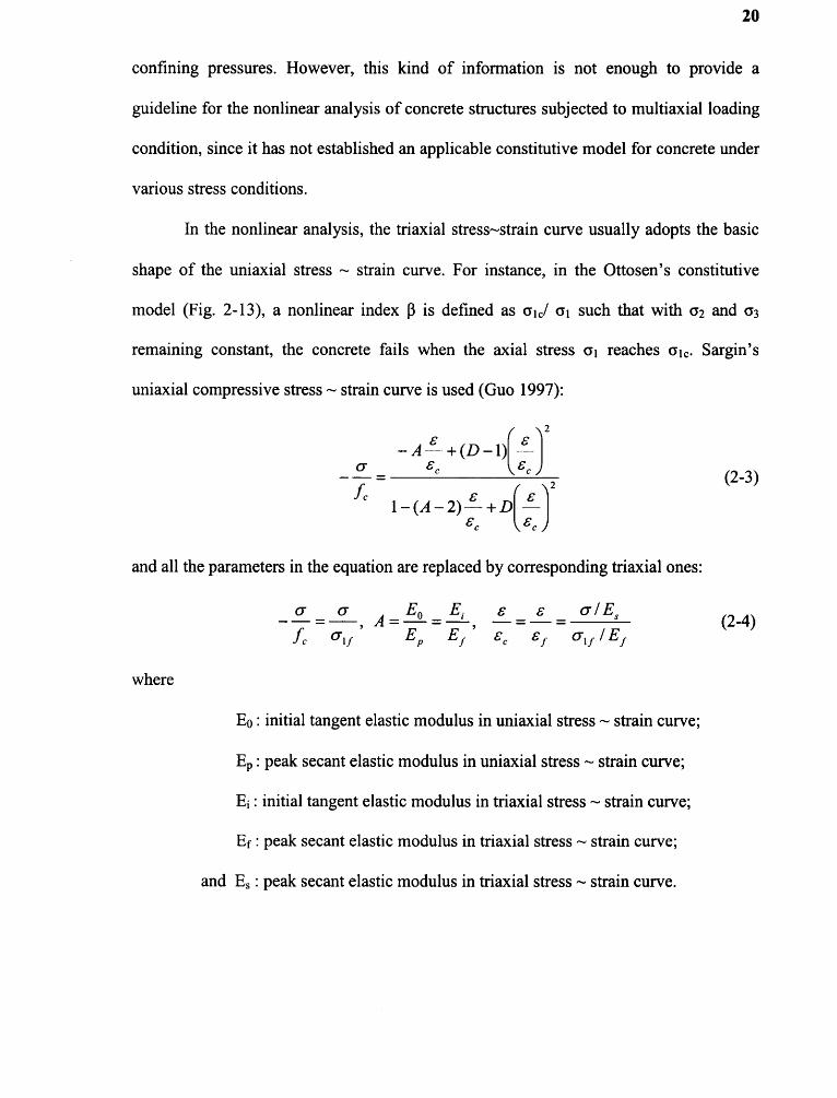
In the nonlinear analysis, the uniaxial stress—strain curve usually adopts the basic
shape of the uniaxial stress ~ strain curve. For instance, in the Ottosen's constitutive
model (Fig. 2-13), a nonlinear index 0 is defined as 6 1c/ al such that with a2 and a3
remaining constant, the concrete fails when the axial stress a 1 reaches al,. Sargin's
uniaxial compressive stress — strain curve is used (Guo 1997):
where
B0 : initial tangent elastic modulus in uniaxial stress — strain curve;
Bp: peak secant elastic modulus in uniaxial stress ~ strain curve;
E1 : initial tangent elastic modulus in triaxial stress ~ strain curve;
Eft .peak secant elastic modulus in triaxial stress ~ strain curve;
and Bs : peak secant elastic modulus in triaxial stress ~ strain curve.
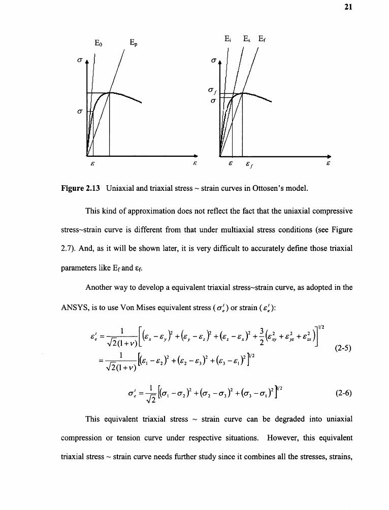
Figure 2.13 Uniaxial and triaxial stress ~ strain curves in Ottosen's model.
This kind of approximation does not reflect the fact that the uniaxial compressive
stress~strain curve is different from that under multiaxial stress conditions (see Figure
2.7). And, as it will be shown later, it is very difficult to accurately define those triaxial
parameters like Bf and Cf.
Another way to develop a equivalent triaxial stress~strain curve, as adopted in the
This equivalent triaxial stress ~ strain curve can be degraded into uniaxial
compression or tension curve under respective situations. However, this equivalent
triaxial stress ~ strain curve needs further study since it combines all the stresses, strains,

22
and Poisson's ratio in the multiaxial stress condition together, and it does not consider the
variation of Poisson's ratio with respect to the stress status. Furthermore, there is a dearth
of information available to prove the similarity between this type of curve and the actual
triaxial stress ~ strain behavior of concrete.
2.2.4 strength of Concrete Under Triaxial stress Conditions
2.2.4.1 Failure Criteria of Concrete In formulating the general failure criterion, a
clear concept of "failure" should be defined. Chen (1982) defined the failure of the
concrete as "the ultimate loading capacity of a test specimen". Failure of the concrete
elements usually occurs under complex loading conditions, therefore, the state of stress at
failure is generally complicated. The study on concrete behavior under multiaxial stress
conditions is essential to develop the general failure criterion.
A failure criterion of isotropic materials based on the multiaxial stress conditions
must be an invariant function of stress state independent of the choice of the coordinate
system by which stress is defined:
However, those three principal stresses can be expressed in term of the
combinations of three principal stress invariants Ii, J2 and J3, and for the brittle material
like concrete, the failure criterion is affected by the hydrostatic pressure (I1/3). Therefore
the failure criterion can be further developed as:

23
It has been found (Guo 1997 and Chen 1982) that the failure surface of concrete
in the three coordinate axes of principal stress has a nearly triangular cross section for the
small stresses and becomes increasingly bulged (more circular) at high hydrostatic stress
conditions. Numerous types of concrete failure criteria have been developed aimed at
defining the shape of the failure surface, and according to the number of variables, the
failure criteria can be categorized into one-parameter, two-parameter, three-parameter,
four-parameter and five parameter models. The heydays of the failure criteria study came
around 1914s, when the famous Druker-Prager criterion, Ottosen criterion, Willam-
Warnke criterion and Hsieh-Ting-Chen criterion were all published. Of them, the 5-
parameter Willam-Warnke criterion was considered to be the most appropriate one to
describe the triaxial behavior of the concrete, so that Chen (1982) stated in early 1980
that "In view of fluctuations of experimental results, there is little need for further
refinements of present failure-surface model".
Right now the 5-parameter Willam-Warnke criterion has been widely used in the
multiaxial FB analysis of concrete elements, including the most acknowledged
commercial computing software — ANSYS. However, the 2-parameter Mohr-Coulomb
criterion has also been successfully applied to concrete due to its simplicity and fairly
reasonable accuracy in some specific cases.
24
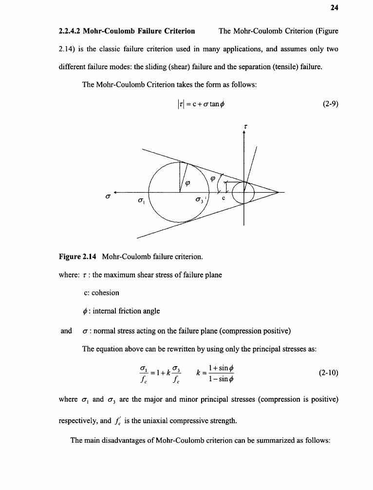
2.2.4.2 Mohr-Coulomb Failure Criterion The Mohr-Coulomb Criterion (Figure
2.14) is the classic failure criterion used in many applications, and assumes only two
different failure modes: the sliding (shear) failure and the separation (tensile) failure.
The Mohr-Coulomb Criterion takes the form as follows:
Figure 2.14 Mohr-Coulomb failure criterion.
where: r : the maximum shear stress of failure plane
c: cohesion
0 : internal friction angle
and a : normal stress acting on the failure plane (compression positive)
The equation above can be rewritten by using only the principal stresses as:
where a 1 and a3 are the major and minor principal stresses (compression is positive)
respectively, and f is the uniaxial compressive strength.
The main disadvantages of Mohr-Coulomb criterion can be summarized as follows:

25
1) The intermediate stress 6 2 is not considered for the failure. This will easily lead to
an obviously erroneous conclusion that the uniaxial and biaxial compressive
strengths of concrete are the same, which is contradictory to the test results (Chen
1982).
2) The tensile and compressive meridians are all straight lines, which become far
deviant from the actual failure surface when the hydrostatic pressure is high. And
the failure surface is not a smooth one, also contradictory to the common
consensus.
3) If tension is considered in this criterion, it will inevitably lead to a relationship
between the uniaxial compressive ( f )) and uniaxial tensile stress (f,)--
10-15. However, according to the early test result of Richart et. al (Chen 1982),
the k is roughly 4.1, which is far less than the value derived by the criterion.
Although the Mohr-Coulomb Criterion has so many apparent weaknesses, due to
extreme simplicity and fair approximate estimation in manual calculations, up until now a
lot of researches have still been undertaken especially on the normal HSC (Xie et. al
1995, Imaran and Pantazopoulou 1996, Cadappa et. al 2001, Ansari and Li 1998, and Lan
1997) and steel fiber reinforced concrete (Nielson 1998 and Pantazopoulou 2001) (Table
2.1).

26
There seems be an obvious disagreement among those researchers on the value of
k, which varies from the lowest 2.6 to a much higher 6.7. Table 2.1 lists the testing results
of k value from some researchers around the world.
Some researchers gave detailed descriptions about the failure mode of the
concrete specimen subjected to lateral confining pressure, which is totally different from
that of the uniaxial compression. Chem (1992) found that the cylinders, with or without
steel fiber, all failed in a shear mode under confining pressures from 1 OMPa to 14MPa
Ansari and Li (1998) stated that the majority of the HSC cylinders
failed in shear as indicated by 45 degree diagonal crack in the specimens under lateral
confining pressure ratios ay/f ranging from 20% to 90%; Guo (1997) used the cubic
concrete specimens and found out that all the specimens were compressed along the axial
direction while stretched in the other two, and there were obvious inclined cracks on
lateral surfaces, which hinted a inclined shearing failure mode; Sfer and Carol (2002)
studied the cylinder failure modes under ay / f from 25% to 180%, and they found that
under relatively lower confinement, the cylinders were likely to fail in a inclined failure
mode, much the same as described by the other people, but when the confining pressure
became lager, a failure of the combination of split and shear seemed to dominate (see
Figure 2.15). It should be noted that in their experiments, Sfer and Carol inserted a
0.1mm thick teflon sheet between the loading platen and the cylinder end to minimize the
end friction.

27

Figure 2.15 Schematic failure mode under different 63 by Sfer and Carol (2002).
It can be seen clearly from all the testing results in Table 2.1 that although there is
a great disagreement on the ultimate strength (k value) of concrete for the Mohr-Coulomb
criterion, the general failure modes are essentially the same—shear failure. If one applies
the Mohr-Coulomb failure criterion with a tension cutoff (maximum strain or stress), this
combined failure criterion will describe the failure of concrete as either tensile or shear
types. The tensile type of splitting fracture is governed by the maximum stress or strain,
while the shear type of slip fracture is controlled by the maximum-shear-stress criterion
of the Mohr-Coulomb criterion.
There is a trend that under lower confining pressures the k value seems to be
higher, and when the confining pressure increases, the slope of the a l cry /
relationship becomes much smoother. It is reasonable since it has been found out that the
meridians of the concrete failure surface are bulged curves rather than straight lines. But
given the extreme simplicity and that most of the applicable cases are under a fairly low
level of confinement, the Mohr-Coulomb criterion can still be employed as a first
estimation of concrete strength under multiaxial compressive status.
However, from the previous research results, one can not find a consensus on the
k value, neither can he draw a conclusion on the influence of concrete strength (

29
confinement level ( c73 / f:), steel fiber introduction and cylinder type to this k value. The
testing results are just scattered, and it is difficult to judge which one is more reliable and
appropriate. Therefore it is of importance to enrich the existing database to provide more
information in determining the k, especially for the HSC and SFHSC under normal
confinement level.
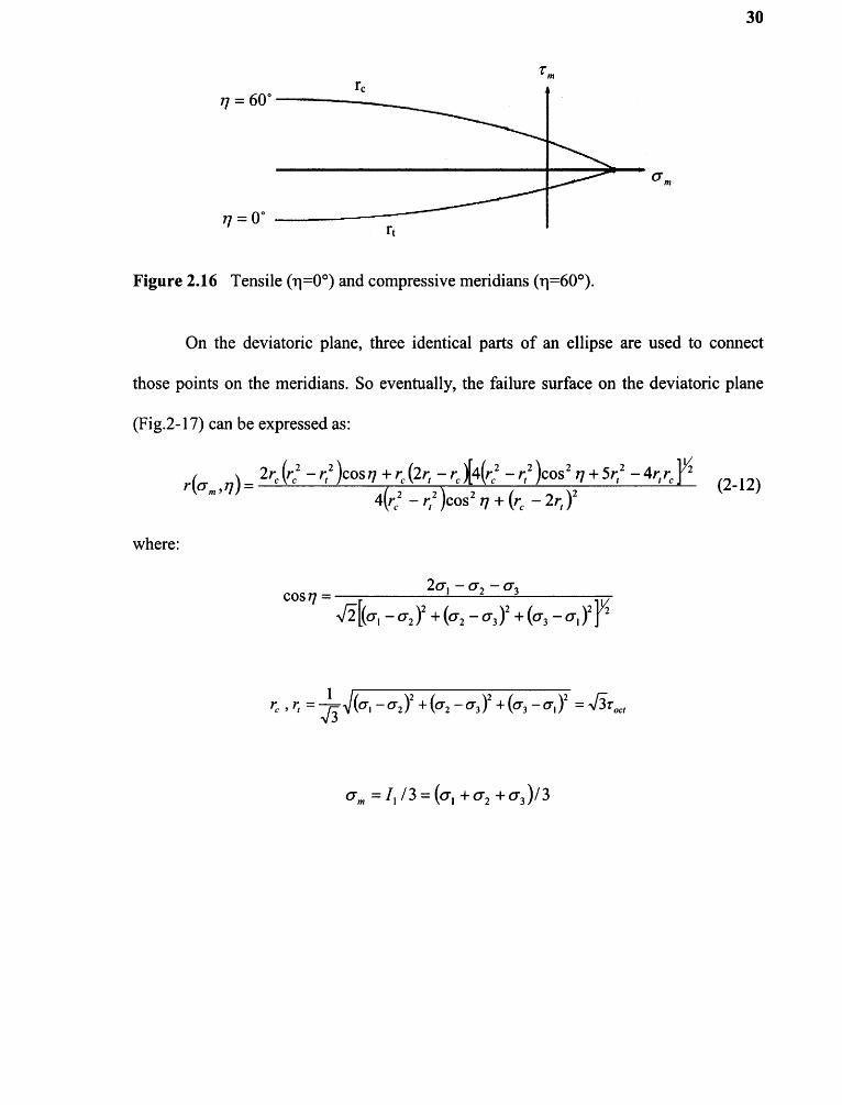
2.2.4.3 Five-Parameter Wiliam Warnke Criterion The tensile meridian
and compressive meridian on the failure surface of the concrete can be expressed as two
to fit the actual curved meridians obtained from the
30
On the deviatoric plane, three identical parts of an ellipse are used to connect
those points on the meridians. So eventually, the failure surface on the deviator plane
(Fig.2-17) can be expressed as:

Figure 2.17 Failure surface and deviatoric plane.
Xie et. al (1995) conducted an extensive study on the compressive meridian of
HSC. In his research, three different HSCs with f of 60.2MPa, 92.2MPa and 119MPa
were tested under triaxial stress condition. The lateral confinement level 6 3 / f was
approximately 50%, and proportional loading path (Figure 2.8) was adopted. The
compressive meridians of those three concretes are shown in Figure 2.18.

32
It can be seen from Figure 2.18 that the compressive meridians of HSC with
different compressive strength are essentially the same, and the curves fit the Willam-
Warnke's meridian expression very well (R2=0.9923-0.9993). There seems to be a trend
that the compressive meridian of concrete with higher strength tends to be lower than
those with lower compressive strength.
Imaran and Pantazopoulou (1996) studied the triaxial behavior for both the
normal strength concrete
confinement level he used is approximately 14%-90% f (Figure 2.19)
Figure 2.19 Compressive meridians of HSC by Imaran (1996).
Ansari an Li (1998) also studied three HSCs with f of 48MPa, 72MPa and
109MPa respectively. The confining pressure used in this research is around 90% f (see
Figure 2.20).

33
Figure 2.20 Compressive meridians of HSC by Ansari and Li (1998).
From Figure 2.20 it shows that the curved meridians of higher strength concrete
seem to be more deviant from that of concrete with relatively lower compressive strength
than in the two previous cases.
If all the triaxial data of the HSC are put together in one graph (see Figure 2.21),
large discrepancies will be observed. It is hard to say which one is more appropriate for
HSC since there are not enough additional testing results available.
Figure 2.21 Compressive meridians for HSC from different researchers.

34
Chem (1992) conducted an extensive program on the triaxial behavior of the steel
fiber reinforced normal strength concrete. He changed the volume ratio of steel fiber in
the concrete from 0%, 1% to 2%, and the concrete compressive strength f was only
around 22MPa. In his tests, the confining pressure level was up to 340% f: . The
compressive and tensile meridians of those concretes are shown in Figure 2.22.
Ishikawa et. al (2000) also studied the tensile and compressive meridians for the
HSC with 1% volume ratio steel fiber and a f of 8OMPa. The results are also listed in
Figure 2.22 to compare with those of Churn's normal strength concrete experiments.
Figure 2.22 Tensile and compressive meridians of steel fiber reinforced concrete.

35
From Chern's results, it can be seen that under relatively lower confining
pressures, all the compressive meridians for concrete with 0%, 1% and 2% steel fiber are
essentially the same. However, when high confining pressure (around 100% f) occurs,
the concrete with higher volume ratio of steel fiber tends to show stronger triaxial
strength behavior. But Ishikawa's equation for HSC is remarkably deviant from Churn's,
even under low confining pressures. One cannot attribute this to HSC since no other
sources of data is available.
However, the tensile meridians for all the concrete, regardless of high strength or
normal strength and with steel fiber or without, follow the same trend.

CHAPTER 3
UNIAXIAL COMPREssION OF sTEEL FIBER REINFORCED HIGHsTRENGTH CONCRETE (sFHsC)
3.1 Lubricated Loading Platen
Generally, as discussed in Chapter 2, there are two kinds of end friction-reducing
measures — brush platen and lubricated loading platen. The brush platen was deemed as
the best testing apparatus to achieve the true uniaxial compression (Mindess et. al 2002
and Guo 1997). It is capable of providing relatively better and consistent testing results
which have been widely quoted by some researchers (Rashid et. al 2002, Kupfer et. al
1969, Van Mier et. al 1997, Gerstie 1981, and Kupfer and Gerstle 1973). However, this
kind of loading platen has a very complicated structure and high cost, and meanwhile,
large deviations still exist in the testing results.
The more economic alternative is to use the lubricated loading platen which is
aimed at decreasing the friction between the loading platen and the end of the concrete
cylinder. Teflon sheet is widely accepted as a practical option for reducing end friction
(Mindess et. al 2002, Guo 1997, Kupfer et. al 1969, Van Mier et. al 1997, Gerstie 1981,
and Kupfer and Gerstie 1973). However, there seems to be no consensus on the effect of
its thickness. In the joint research program coordinated by RILEM (Van Mier et. al
1997), a variety of thickness from 0.05 mm to 1.0 mm were used in the laboratories
worldwide, while no definitive conclusion concerning thickness has been made. It has
only been found that there is no apparent difference between the teflon sheets with the
thickness of 0.125mm and of 0.250mm. Researchers in Tsinghua University of China
(Guo 1997) recommended that the teflon sheet with a 2mm thickness should be used.
36

Figure 3.1 Designed lubricated loading platen.
A specially designed lubricated loading platen as shown in Figure 3.1 is used in
this study. Two 0.125mm (0.005 in.) thick teflon sheets are used to exploit the much
lower friction between them. The thin 0.015 mm (0.0006 in.) thick aluminum foil has
twofold functions. First, bearing grease can be thinly applied between this foil and the
teflon sheet without inducing the possible reversal of boundary restraint (Van Mier et. al
1997) as has been discussed in Chapter 2. And secondly, since the a / E of the aluminum
is quite close to that of the HSC, it will lead to a almost identical lateral expansion for
both the concrete specimen and the aluminum foil under uniaxial compression.
3.2 Lateral strain Measurement
In this study, circumferential extensometers were used to detect the lateral strain of the
concrete cylinder. The circumferential extensometer is a specially designed "clip gauge"
for measuring the average lateral expansion along the whole circumference of the
cylinder, and it is advantageous over the normally used electrical strain gauge which can
only catch the length change of a small portion of the total cylinder circumference. Given
the remarkable heterogeneity of the concrete and highly localized deformation, the

38
circumferential extensometer is apparently much more reliable to provide accurate and
consistent average circumferential deformations, which can then be converted easily into
the lateral strains.
A solid stainless steel rod with a diameter of 8"(200mm) and a height of
8"(200mm) was used to verify the accuracy of the circumferential extensometer, which
was installed right at the mid-height of the rod together with an electrical strain gage
along the circumferential direction. A 900 kN compressive load was applied to the rod
and the lateral strains detected by the circumferential extensometer and strain gage are
shown in Figure 3.2.
Figure 3.2 Relationship between the lateral strains from the circumferentialextensometer and strain gage.
It can be clearly seen from Figure 3.2 that the lateral strains from circumferential
extensometer and strain gage exhibit a terrific linear relationship. The slope is slightly
less than 2.0 just because those two measuring instruments could not be perfectly
positioned symmetrically opposite to each other along the height of the specimen.
39
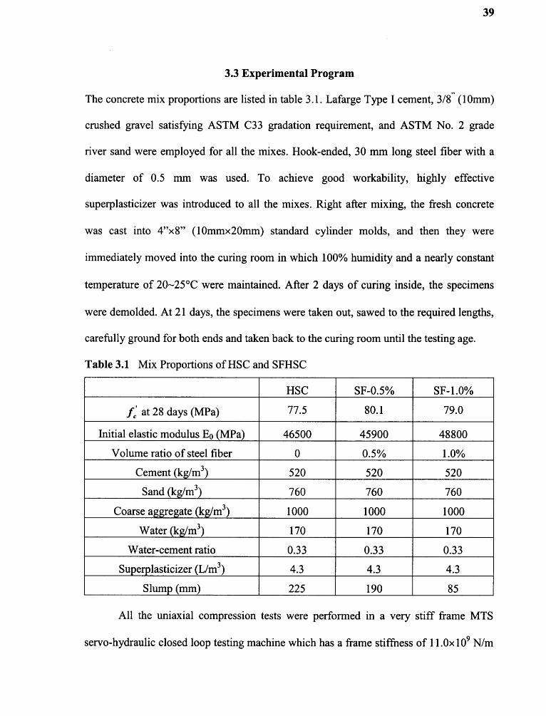
3.3 Experimental Program
The concrete mix proportions are listed in table 3.2. Lafarge Type I cement, 3/8 (20mm)
crushed gravel satisfying ASTM C33 gradation requirement, and ASTM No. 2 grade
river sand were employed for all the mixes. Hook-ended, 30 mm long steel fiber with a
diameter of 0.5 mm was used. To achieve good workability, highly effective
superplasticizer was introduced to all the mixes. Right after mixing, the fresh concrete
was cast into 8"x8" (20mmx2Omm) standard cylinder molds, and then they were
immediately moved into the curing room in which 200% humidity and a nearly constant
temperature of 20-25°C were maintained. After 2 days of curing inside, the specimens
were remolded. At 22 days, the specimens were taken out, sawed to the required lengths,
carefully ground for both ends and taken back to the curing room until the testing age.
All the uniaxial compression tests were performed in a very stiff frame MTS
servo-hydraulic closed loop testing machine which has a frame stiffness of 22.0x209 N/A
3.4 Experimental Results
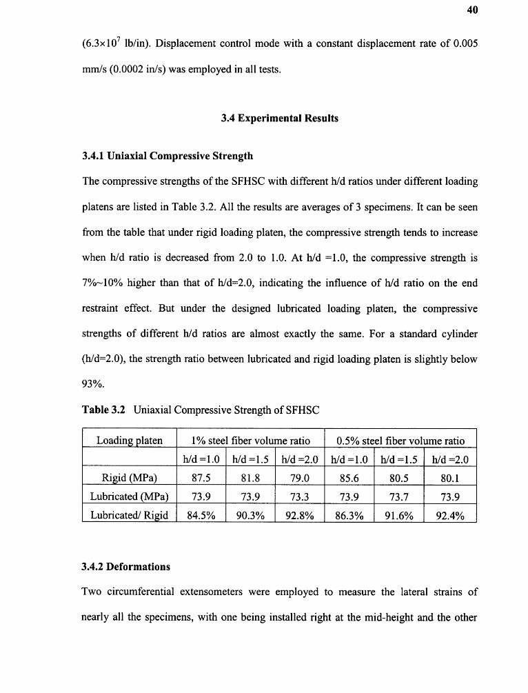
3.4.1 Uniaxial Compressive strength
The compressive strengths of the SFHSC with different hid ratios under different loading
platens are listed in Table 3.2. All the results are averages of 3 specimens. It can be seen
from the table that under rigid loading platen, the compressive strength tends to increase
when h/d ratio is decreased from 2.0 to 2.0. At b/d =2.0, the compressive strength is
7V0-20% higher than that of hld=2.0, indicating the influence of h/d ratio on the end
restraint effect. But under the designed lubricated loading platen, the compressive
strengths of different h/d ratios are almost exactly the same. For a standard cylinder
(h/d=2.0), the strength ratio between lubricated and rigid loading platen is slightly below
93%.
3.4.2 Deformations
Two circumferential extensometers were employed to measure the lateral strains of
nearly all the specimens, with one being installed right at the mid-height and the other

41
approximately 2/6h from one end. The purpose is to demonstrate whether the specimen
has a tendency of a uniform lateral expansion under the uniaxial compression. Axial
extensometers were used to detect the axial strains, with 8 inch gage length for h/d = 2.0
and 2 inch gage length for hid = 2.0 and 2.5. The axial and lateral strains at peak load for
specimens with different hide ratios under two types of loading platens are shown in Table
3.3, Table 3.8 and Figure 3.3, respectively.
Under rigid loading platen, for h/d=2.5 and 2.0, the peak lateral strains at the mid-
height of the specimen are 37%-65% larger than those correspondingly near the end.
These notable differences clearly demonstrate the considerable end restraint imposed to
the specimen by the rigid loading platen. But once the designed lubricated loading platen
was employed, those strain differences were greatly diminished (see Figure 3.3).

42
Figure 3.3 Lateral strains SFHSC at peak load.
Under the lubricated loading platen, there is a general trend that at h/d=2.0, the
peak lateral strain at the mid-height is less than that near the end, and at hld=2.5 a reverse
situation occurs. However, the held of 2.5 seems to be the transition point where the lateral
strains at the mid-height and end are essentially the same. Thus in terms of uniform
lateral expansion, hld=2.5 tends to be more appropriate in providing the true uniaxial
compression test.
Figure 3.8 shows the stress ~ strain curves of 2% fiber volume ratio SFHSC
cylinders with b/d =2.5 under both rigid and lubricated loading platens. It can be clearly
seen that under lubricated loading platen, the lateral strains at both mid-height and end
comply with each other pretty well not only before but also at and after peak. However,
those lateral strains under rigid loading platen start to diverge from each other around
95% of the peak load, and after peak, the difference increase tremendously. The 5.5%
fiber volume ratio SFHSC also behaves in the same manner.

43
Figure 3.4 Uniaxial stress ~ strain curve of 2% fiber volume ratio SFHSC (h/d=2.5).
The lateral strains measured at the mid-height of the specimens, as have been
done by most previous researches in studying the Poisson's ratio and bulk modulus, are
remarkably different under two different loading platens. For instance, the average mid-

44
height peak lateral strain of the 2% fiber volume ratio SFHSC with h/d=2.5 was
apparently reduced from 2142 [Ls under rigid loading platen to 2588 I.L under the
lubricated one — a considerable 32% decrease, but the corresponding axial strains only
experienced comparatively a much lower 8% reduction.
3.4.3 Volume Change and Bulk Modulus K
Bulk modulus K represents the volumetric stress and strain relationship of concrete and is
defined as:
Testing data under lubricated loading platen and a hid ratio of 2.5 were adopted to
achieve the variation of bulk modulus K under different stress conditions, since they
would be comparatively consistent with the uniform lateral expansion under uniaxial
compression, as can be seen from Figure 3.3. The results are shown in Figure 3.5 and
Figure 3.6 respectively.
The K variations of those two types of steel fiber reinforced SFHSC follow the
same trend. Initially, a linear elastic response between the octahedral stress cod and
volume change (360,, ) develops up to approximately 95% of the ultimate strength, and
then the concrete starts to dilate. After peak, cr ock, tends to decrease linearly with the
volume expansion of the concrete, with a K about 5%-6.6% of that in the initial elastic
volumetric contraction stage (K0). Therefore, it may be fairly reasonable to take only two
constant bulk moduli K for before and after peak respectively in the analysis.

Figure 3.6 Bulk modulus of 5.5% fiber volume ratio SFHSC before and after peak
(el lecu - - 2 ).
45

46
However, it has to be noted that the deformation of the concrete becomes quite
volatile when the cracks inside the concrete fully develops under uniaxial compression,
which will greatly influence the measurement of the axial strain since the length of the
gage can not catch the localized damage of the cylinder. It has been observed from all the
tests that when the axial strain is less than two times of the peak axial strain, all the axial
stress ~ strain curves are smooth and free from shape irregularities, which will provide
more reliable information for the volumetric change. That's why a limit of
has been stipulated.
3.4.4 Poisson's Ratio
The Poisson's ratio of concrete is defined as the ratio of lateral strain to axial strain under
the uniaxial compression or tension. Most of the published data (Persson 2999, Rashid
2552, and Gao et. al 2997) were attained by employing the ASTM C 869, in which the
direct strain measurement was performed in the standard uniaxial compression test under
a compressive stress of 85% f:. Normally, a constant Poisson's ratio for concrete is
assumed, which is reasonable under certain low stress levels when the concrete exhibits
essentially linear elasticity. However, Mindess, Young and Darwin (2502) stated that, at
approximately 14% of the f:, the microcracking inside the concrete parallel to the
direction of the stress starts to develop much faster up until the failure, thus inducing a
highly inelastic feature within that stage, which may greatly affect the apparent Poisson's
ratio .
Depending on the computer analysis model, either secant or tangent Poisson's
ratio is employed. For the normal strength concrete, the classic description of the secant

47
Poisson's Ratio variation with stress condition is from Ottosen's constitutive model
(Ottosen 2979) (Fig. 3-7), in which stress index is predefined as fi = 6, / o-if such that
with 62 and a3 being constant, concrete failure will occur when a, reaches w aif . The
secant Poisson's Ratio a, can be expressed as following:
Figure 3.7 Poisson's Ratio (secant) variation in Ottosen's model.
A cubic polynomial expression of tangent Poisson's ratio under uniaxial
compression with respect to the ratio of the axial strain ( c e ) to the peak axial strain (e)
was proposed by Kupfer, Hilsdorf, and Rusch (2969):

48
where: a0 is the initial tangent Poisson's ratio
From this equation, tangent Poisson's ratio will start to rise dramatically after
Mc / =55%. Under a0 =5.25, the tangent Poisson's ratio at peak will reach 2.22,
demonstrating a great volatility of Poisson's ratio near the peak.
However, for the SFHSC, there is' a dearth of information available concerning
the Poisson's ratio variation under different stress conditions. And in most of the previous
research programs, especially those using cylinders, end restraints were not taken into
consideration and concrete specimens were just assumed to be subjected to uniform
lateral expansion. This is untrue since it has been demonstrated by many researchers
(Mindess et. al 2552, Guo 2997, and Van Mier et. al 2997) that there exists a considerable
friction between the rigid loading platen and specimen end, which acts as a lateral
confinement at the specimen end, thus increasing the strength of the specimen. Mindess,
Young and Darwin (2552) revealed that for a standard cylinder with hide =2.5, only the
small central portion of concrete is in the true uniaxial compression, while the remainder
virtually is in triaxial stress status (see Figure 2-2 (a)). Basically, the concrete does not
possess a "compression failure" since the tensile strain capacity of concrete is much less
than its compressive counterpart. Under a true uniaxial compression status, due to the
Poisson's effect, the concrete should theoretically have a splitting tensile failure mode as
shown in Figure 2-2(b).
Figure 2-2(a) is the typical cone failure of a standard cylinder (hld=2.0)
compression test from which most of the existing data concerning Poisson's ratio
variation are achieved. It can be clearly seen that only the small central portion of
concrete is in true uniaxial compression. Because the strain measurement instruments are

49
mostly installed on the surface of the specimen, the tested axial and lateral strains are
actually the responses of the concrete portion which is in a complicated stress condition,
especially near the failure. Therefore, to attain an accountable Poisson's ratio, it is of
great importance to reduce the end restraint for the concrete to reach a "true" uniaxial
compression status.
As shown in previous sections of this chapter, concrete specimen with hld=2.5
under designed lubricated loading platen is more likely to provide the uniform lateral
expansion under uniaxial compression, therefore this kind of specimens were employed
to study the Poisson's ratio variation with stress condition. Figures 3.8 and 3-9 show
these variations for both 2% and 0.5% fiber volume ratio SFHSC under different loading
platens until peak load. It can be clearly seen that the secant Poisson's ratios below 14%
of peak stress and the tangent Poisson's ratios below 50% of peak stress for both of the
two concretes under different end conditions are essentially the same, to which a constant
of 0.20-0.22 can be applied. Beyond those ranges, the Poisson's ratios under lubricated
and rigid loading platens experience increasing divergence. For instance, right at the
peak, secant Poisson's ratio ranges from 0.36 to 0.82 under lubricated platen compared
with 0.63 to 0.72 under rigid platen, and the difference between the two tangent Poisson's
ratios becomes even wider, with 0.85 to 2.25 under lubricated platen versus 3.22 to 8.02
under rigid platen.
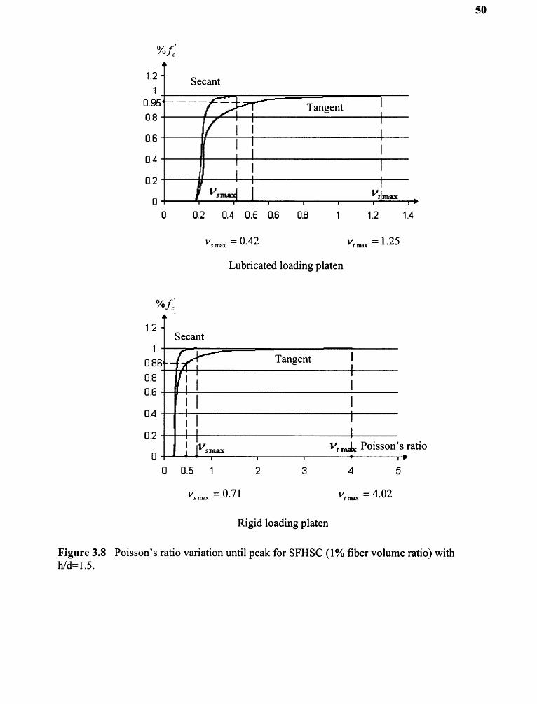
Figure 3.8 Poisson's ratio variation until peak for SFHSC (2% fiber volume ratio) withh/d=2.5.

Figure 3.9 Poisson's ratio variation until peak for SFHSC (0.5% fiber volume ratio) withhld=2.5.
51

52
Another issue deserving discussion is the place where a tangent Poisson's ratio of
0.5, the threshold indicating the end of concrete contraction, occurs. Under the rigid
loading platen, it occurs around 83%-86% of the peak stress compared with
approximately 95% under lubricated platen, which coincides with the point of zero
incremental volume change in the graph of octahedral normal stress versus volume
change (Figures 3.5 and 3-6) and represents the start of dilatation. Gristle (2982) also
reported that in the case of biaxial compression, concrete dilatation occurred immediately
preceding the failure, but he acknowledged there existed a lot of contradictory results
which indicated that this dilatation occurred at stress levels of 14% to 85% of failure. He
attributed this discrepancy to the possible influence of the load application and strain
measurements.
As discussed above, when the stress level is below 14% of the failure, the secant
Poisson's ratio of SFHSC can be taken as a constant of 0.2. The secant Poisson's ratio at
peak falls in a range from 0.36 to 0.82, which is quite close to that stipulated in the
Ottosen's constitutive model for ordinary concrete. Eventually, the variation of secant
Poisson's ratio of SFHSC under uniaxial compression can be expressed as following:
Figure 3.20 shows the tangent Poisson's ratio variation for SFHSC before peak
under true uniaxial compression (lubricated loading platen) as compared with the
equation proposed by Kupfer et. a2(2969) for ordinary concrete under biaxial loading. It

53
is quite apparent that Kupfer's equation is applicable to SFHSC when the initial tangent
Poisson's ratio vo is taken as 0.2. Elwi and Murray (2979) proposed that a limit value of
0.5 be placed on the tangent Poisson's ratio and insisted that this yield realistic estimates
of stress.
Figure 3.10 Tangent Poisson's ratio variation for SFHSC before peak compared withKupfer's equation (2969).
Figure 3.22 shows the variation of tangent Poisson's ratio of SFHSC after failure
under true uniaxial compression (lubricated loading platen). It seems fairly reasonable to
adopt a constant of 2.35 for a, after failure ( e 1 le< 2.5 ).

63 / Mct•2 -
1.0 -
1.6 -
14-
1.2
-1-
0.8 -
0.6 -
0.4 -
0.2 -
0 81 / sect
54
0 0.5 1 1.5 2 2.5
2% steel fiber — — 0.5% steel fiber
Figure 3.11 Tangent Poisson's ratio for SFHSC after peak (s 1 1 Mct, < 2.5 ).

CHAPTER 4
TRIAXIAL COMPREssION TEsT sETUP
4.1 Testing Apparatus
All the triaxial compression tests in this study for both HSC and SFHSC were performed
by the MTS 820 material testing system. It is a very stiff frame MTS servo-hydraulic
closed loop testing machine with a frame stiffness rated at 12.0x20 9 N/A. It has a
8600KN (2,000,000 albs) load capacity with the triaxial cell being able to apply up to
88MPa (12ksi) confining pressure. The test setup is shown in Figure 8.2.
Before the triaxial compression test starts, the pressure chamber in Figure 8.2 is
filled with pressure oil by the pressure intensifier of the MTS system, and then the
intensifier will press the oil to create the target confining pressure. In this study, the axial
compressive stress will be always designated as a, while the confining pressure as a2
and a y , so it can be clearly seen that actually this testing setup can only provide uniform
confining pressures ( a 2 = 0- y ). However, the advantage of this machine is that it can be
purposely programmed to perform various kinds of combinations of axial stress a l and
confining pressure a 3 on the concrete specimen, including cyclic loading.
In order to get a successful triaxial compression test done, three aspects need to be
meticulously taken care of, namely the specimen, extensometers (axial and
circumferential) and the isolation plastic sleeve.
55

Figure 4.1 uniaxial test setup.
4.2 specimen Treatment
The surface condition of the concrete specimen is vital to a successful uniaxial
compression test, since under high oil pressures, even a normal air void hidden right
below the surface of the specimen which is innocuous under uniaxial compression will be
easily penetrated through by the pressurized oil. This may cause a punching failure of the

57
isolation sleeve, which will lead to a direct contact between the specimen side surface
and the confining oil. The oil can then penetrate through any possible cracks occurring
under compression and acts as a splitting force inside the specimen.
To avoid this negative scenario, two measures were adopted in this study. First, a
highly effective superplasticizer Sika2000 was employed instead of the previous Sika86
in the triaxial compression concrete mixture. Sika2000 is capable of producing flowable
concrete mixture with high workability and consistency under low water to cement ratio,
thus greatly decreasing the density of relatively large air voids beneath the side surface.
However, even this is not enough to totally eliminate those voids, especially when the
slump of the fresh concrete was severely reduced with the introduction of steel fiber at
2% volume ratio. In this case, the second measure is a must, although tedious and
harrowing. The side surface of the specimen was scratched thoroughly using a steel blade
until all the hidden voids could be clearly seen, and then all the relatively large voids
(with a diameter roughly larger than 0.5mm) were filled up with cement paste. After this
work was done, the specimen was taken back to the curing room where it would stay
until the test.
To achieve a good contact between the specimen and the loading platen, both
ends of the specimen were carefully ground. To make the 100mmx 250mm (8x6 in.)
specimen, a 100mmx200mm (8x8 in.) was cut at the top to eliminate the potential weak
layer due to vibration during casting, and then it was ground to the specified length.
Chapter 3 shows that 100mmx 250mm (8x6 in.) specimen with ground ends under
designed lubricated loading platen was likely to produce a uniform lateral expansion even
after peak load under uniaxial compression. Thus the same setup was also used in the

58
triaxial compression test, and ordinary 100mmx200mm (8x8 in.) specimens were also
employed to make the comparisons of the experimental results between these two
cylinders.
4.3 Axial and Circumferential Extensometers
Axial and circumferential extensometers have a remarkable advantage over traditional
strain gage in measuring large deformations, which is extremely important under triaxial
compression where the axial and lateral strains can both be large compared with their
uniaxial counterparts. However, the measurement accuracy of these extensometers needs
to be addressed before the tests in order to maintain the credibility of the experimental
results.
The manufacturer (MTS company 1998) clearly stipulates that if the difference
between the shunt calibration voltage value and the reference one of the extensometer is
less than 15 my, the measurements from the tests can be satisfactorily accurate. So in this
study, shunt calibration was made before each triaxial test, and it was found that the error
of the circumferential extensometer was consistently within that range but that of the
axial extensometer was slightly away with a maximum difference of 30 my. However,
given that the total reference voltage value is 9.33 v, this slightly larger difference will be
likely not to cause any appreciable experimental errors.
Another checkup with the extensometers is to use a solid steel rod to perform a
standard compression test, like the one described in Chapter 3. Hereby another set of
steel rod uniaxial compression test results is provided in Figure 8.2 and Figure 8.3,
respectively.

59
Figure 4.2 Axial stress — axial strain of steel rod under uniaxial compression.
It can be found from those two figures that the elastic modulus and the Poisson's
ratio of the steel rod are 205,000 MPa and 0.2667 respectively, which fall into the
reasonable range for this material. The slight difference from the reference value may be
attributed to the installation positions of the extensometer on the specimen. Again, almost
perfect linear relationships were achieved for those two graphs.
Figure 4.3 Lateral strain — axial strain of steel rod under uniaxial compression.

60
As a conclusion, using the axial and circumferential extensometers to measure the axial
and lateral strains can give much confidence to the measurement accuracy of the tests.
4.4 Plastic Isolation sleeve
4.4.1 selection and Mechanical Properties of the sleeve
Probably the most important task of setting up a triaxial compression test is to select the
appropriate isolation sleeve to protect the highly pressurized oil from a direct contact
with the side surface of the specimen.
Although the side surface of the specimen has been treated carefully as is
mentioned above, there may still be some air voids unrevealed during the surface
treatment, leaving a high probability of oil penetration under high confining pressure.
Therefore, firstly the selected isolation sleeve should have a high tensile strength together
with a good ductility. Secondly, the selected isolation sleeve should not be so thick as the
rubber sleeves commonly used by many researchers in conducting the triaxial
compression tests, which will be hard for the accurate measurements of strains. And
finally, this isolation sleeve should be in tight contact with the side surface of the
specimen after installation for the sake of (axial and circumferential) strain measurement
and oil infiltration prevention. After a time-consuming search and comparison, the PVC
transparent heat-shrink tubing with a original inner diameter of 100mm (8 in.) and a wall
thickness of 1.85 mm (0.073 in.) was adopted in this study.
The tensile stress ~ strain curve of this PVC material is shown in Figure 8.8.

61
Figure 4.4 Tensile stress ~ strain curve of the PVC material.
The tensile capacity of this PVC is larger than 50% (the strain measurement
stopped at the maximum capacity of the extensometer) and the ultimate tensile strength is
around 50 MPa. Ansari and Li (1998) used another kind of heat-shrink tubing which has
a maximum tensile capacity of 30 MPa, much lower than that of this study.
Installation of this tubing is quite easy. The surface-treated specimen is placed
into this sleeve and two 100mm-diameter loading platens with end friction reducing
measures (see Chapter 3) are also inserted into the sleeve with one at each end of the
specimen. Then the assembly is heated inside an electrical oven for about 5 min. at a
sustained temperature of 180-150 °C. After heating, the specimen is left at room
temperature to cool down. The final procedure is to wrap the electrical tape around the
joint of the isolation sleeve and the loading platen to provide additional sealing control.
When it is all done the specimen is ready to go for a tnaxial compression test.

62
Due to all of the careful specimen treatment considerations, only 2 out of more
than 30 triaxial compression specimens failed before the experiment was completed, for a
successful rate well above 90%.
4.4.2 Elimination of Deformation of the sleeve from the Total Lateral strain
It is obvious that the existence of the PVC sleeve affects the measurement of the total
lateral strain, especially under high confining pressures when the wall of the sleeve is
squeezed in the radial direction to cause a thickness decrease.
This effect is evaluated using two triaxial compression tests of the steel rod, one
with the isolation sleeve and one without. During the test, the ratio of the axial stress to
confining pressure is kept as 8.382 all the way up to the confining pressure of 14 MPa,
which is exactly the maximum confining pressure the true concrete specimen will
undergo. Figure 8.5 shows the lateral (circumferential) strains in those two different
situations and the final radial contractions of the sleeve under different confining
pressures are also calculated.
The contribution of the contraction of the PVC sleeve under different confining
pressure a y to the total lateral strain can be expressed as follows:
where epvc is the lateral strain (in contraction) of the PVC sleeve under confining
pressure 63.
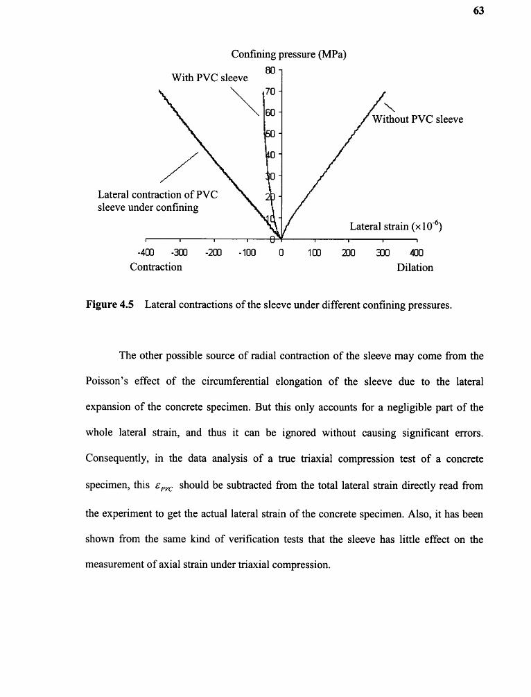
63
Figure 4.5 Lateral contractions of the sleeve under different confining pressures.
The other possible source of radial contraction of the sleeve may come from the
Poisson's effect of the circumferential elongation of the sleeve due to the lateral
expansion of the concrete specimen. But this only accounts for a negligible part of the
whole lateral strain, and thus it can be ignored without causing significant errors.
Consequently, in the data analysis of a true triaxial compression test of a concrete
specimen, this epic should be subtracted from the total lateral strain directly read from
the experiment to get the actual lateral strain of the concrete specimen. Also, it has been
shown from the same kind of verification tests that the sleeve has little effect on the
measurement of axial strain under triaxial compression.

CHAPTER 5
ANALYsIs OF TRIAXIAL COMPREssION TEsT REsULTs OF HIGHsTRENGTH CONCRETE (HsC)
5.1 Experimental Program
The mix proportion of the HSC for triaxial compression test is the same with that of the
uniaxial compression test (Chapter 3). However, since high-quality washed aggregates
(sand and crushed gravel) had been used up in the previous tests, relatively low-quality
sand and crushed gravels had to be adopted for the triaxial specimens instead, which
attributed to the decrease of the standard compressive strength L IB (down from 77.5 MPa
to 68.5 MPa) and the initial elastic modulus E0 (down from 86500 MPa to 80140MPa).
The specimen curing, treatment and test setup have already been discussed in
Chapter 8. In this triaxial compression test, 100x200 mm (8"x6") concrete cylinders with
both ends ground were tested under the designed lubricated loading platen mainly
through two different load paths: T-1 and T-2. The load application procedures of those
two load paths are shown Figure 5.1.
64

65
The difference between T-1 and T-2 lies in the different 6 3 / a, ratios before the
target confining pressure a y is reached. The ratio of 6 3 / a l is 1/2 for T-1 and 1/6 for T-
2, respectively. In both load paths, load control was employed before the target confining
pressure with the increasing rate of a y being 7 MPa/min for T-1 and 3-8 MPa/min for T-
2 respectively. After the target o - y , both paths adopted displacement control all the way
until the failure (including strain softening) of the specimen. The displacement rate for
both cases fell in a range from 0.005 mm/s (0.0002 inks) to 0.006mm/s (0.00025 inks).
The displacement control was applied in order to get the descending branch of the triaxial
stress ~ strain relationship.
5.2 Failure Criterion
5.2.1 Mohr-Coulomb Criterion
According Mohr's criterion, material's failure will occur for all stress states at which the
largest of Mohr circles is just tangent to the envelop defined by I'd = f (o-) . If this

66
envelop is set to be a straight line as shown in Figure 5.2, it will become the Coulomb's
equation:
where c is the cohesion and 4 is the internal-friction angle of the material. The
intermediate principal stress a 2 will have no influence on the failure.
Figure 5.2 Mohr-Coulomb failure criterion.
If the uniaxial compressive strength f: is considered and simple geometric
relationship is exploited from Figure 5.2, Equation (5-1) can be transferred into the
following form:
The sign convention used hereafter is that the compression is positive and
al __ a2 ?.. 63 . In this part of experiment, a total of 3 uniaxial compression tests and 18
triaxial compression tests under various confining pressures were performed. The details
of the experiment, including the specimen size, end treatment, load path, and testing

67
control mode have been already discussed earlier in this chapter. The test results for
Mohr-Coulomb Criterion are listed Table 5.2 and Figure 5.3.
Figure 5.3 Mohr-Coulomb failure criterion for HSC.
It can be seen clearly form Table 5.2 that due to the painstakingly careful pre-
experiment quality control work such as the raw material preparation, the concrete
mixing, the specimen making and end grinding, the successful isolation membrane

68
selection and its proper installation, the efficient end friction reducing measure, and the
meticulous exploitation of the advanced MTS system, the triaxial compression testing
results turn out to be highly consistent. For instance, under the same confining pressure of
18MPa and the identical load path, the triaxial strengths of 3 specimens are 132.7MPa,
138.9MPa and 135.5MPa respectively, resulting in a deviant error from the mean value
less than 2%.
In this experiment, the maximum confining pressure is 14MPa (8 ksi), roughly
85% of the uniaxial compressive strength f: of the HSC. This confinement level is well
above most of the values used for HSC with the same strength grade in previous
researches discussed in Chapter 2 (Table 2.1). From this study, k is 8.5 and
compressive strength to tensile strength of the HSC should be equal to 8.0. This value is
far lower than the well-accepted fc / ft ratio of 1015, thus the Mohr-Coulomb criterion
is not applicable when tensile failure is involved. Also, it is found from Equation (5-3)
that the internal friction angle 0 of the HSC is 36.9°.
5.2.2 Willam-Warnke Failure Criterion
As discussed in Chapter 3, Willam-Warnke failure criterion is probably the most widely
used criterion in concrete. It has been adopted in the popular finite element analysis
software ANSYS. The meridian equation takes the form of follows:

69
And for the HSC, this study shows that the compressive meridian of Willam-
Warnke failure criterion takes the form of:
Figure 5.8 shows the comparison of the compressive meridians of HSC in terms

Figure 5.4 Compressive meridian of Willam-Warnke failure criterion for HSC.
Figure 5.5 Comparison of compressive meridians of HSC.
From Figure 5.5, it can be seen that under approximately the same compressive
strength grade, the compressive meridians from Xie, Pantazopoulou and this study

71
comply with one another very well while that of Ansari deviates from the mainstream,
especially at the higher end of the octahedral stresses.
In this study, due to the upper limit of the testing machine to apply the confining
pressure and the relatively high compressive strength of concrete, the ratio of a o to f:
is lower than 2.0. Using the low strength concrete ( =20.5 MPa), Chem (1992)
performed a comparatively higher confining pressure (380%f ) and reached a (r od to
f ratio of 5.6. The comparison between those two meridians is shown in Figure 5.6.
Figure 5.6 Comparison of meridians from Chem and this study.
Figure 5.6 indicates that even though their strengths are quite different from each
other, the compressive meridians of the high and normal strength concrete fairly follow
the same trend, especially at low cr ock, to f ratios. For the normal strength concrete,
when the o f ratio reaches 8.0, the compressive meridian starts to become more
curved. It is still unclear whether HSC will exhibit the same kind of feature since no
experimental data is available around that extremely high confining pressure region.

72
5.3 Triaxial stress — strain Relationship
5.3.1 strains at Peak stress under Triaxial Compression
Under different confining pressures from 0 to 14 MPa (8ksi), the relationship between the
axial strain and lateral strain at peak is shown in Table 5.8 and Figure 5.7.
Table 5.8 shows that with the increasing of the lateral confining pressure a 3 , the
axial and lateral strains at peak both increase dramatically. The relationship between the

73
Figure 5.7 Peak strain ratio versus confining pressure level for HSC.
There is also a close relationship between the lateral peak strain 6 3, and axial
peak strain e l , when the confining pressure increases (as shown in Figure 5.8), which can
be expressed as follows:
Figure 5.8 Relationship between axial and lateral strains at peak for HSC.

74
From Table 5.8, it seems that different load paths do not have an appreciable
influence on the axial strength, the peak axial strain and the peak lateral strain, which
agrees with Guo's findings (1997).
5.3.2 Axial stress versus strains under Various Confining Pressures
Under load path T-1 and different confining pressures from 0 to 56 MPa, the axial stress
strain curves of HSC under triaxial compression are shown on Figure 5.9.
Under load path T-1, the confining pressure cry and axial pressure crib were
gradually applied to the specimen simultaneously with a constant stymy to 6l ratio of 1/2
until the target confinement was reached. Therefore, due to the Poisson's effect, the axial
strain development was contained to some extend by the confining pressure 6y, which

75
resulted in steeper initial slopes of the axial stress — strain curves under triaxial
compression than that of the uniaxial counterpart, as can be seen on Figure 5.9.
However, the load path T-1 is by no means close to the proportional load path
since right at the target confinement 6y, axial pressure 6l is far away from its peak value
6 l ,. For instance, when the target confining pressure a y (28 MPa) is reached, al is only
14 MPa, only 31% of the peak value of 180.2 MPa. In this case, load path T-2 will be
more appropriate in simulating proportional loading in which a constant 6 y to 6 l ratio of
1/6 is maintained until the target confinement. At target a y of 21 MPa and 28 MPa, 6l is
126MPa (80%aic ) and 168MPa (93.4%ale) respectively. The comparison of the triaxial
stress ~ strain curves between those two load paths under 6 y=28 MPa is shown in Figure
5.10.
Figure 5.10 Comparison of triaxial stress ~ strain curves under different load paths.
From Figure 5.10, those two sets of stress ~ strain curves under load path T-1 and
T-2 are essentially the same in terms of the peak axial stress al e, peak axial strain 61 c and

76
peak lateral strain sync. The slight difference between those curves may be attributed to the
different Poisson's effect from the lateral confinement which is larger under T- 1.
5.3.3 Octahedral stress – strain Relationship
The triaxial stress – strain curves discussed above are more qualitative than
quantitative, and they can only reflect the general trend of the stress ~ strain variation
under some specific load conditions. In order to be applicable in the more complicated
practical cases, other types of strain ~ strain curves need to be developed. Octahedral
stress ~ strain relationship is among them.
There are two types of octahedral stress ~ strain relationships—octahedral normal
stress ( a„,f ) versus volume change (3 eoc ) and octahedral shear stress ( r oot ) versus
engineering octahedral shear strain ( C oca, ), where
Under the stress and strain increments, the tangent bulk modulus K t and tangent
shear modulus At can be expressed as follows:
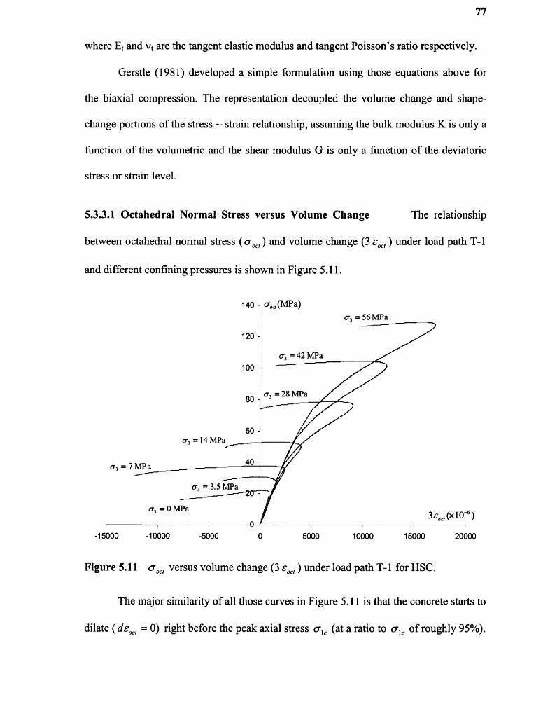
77
where Et and Ft are the tangent elastic modulus and tangent Poisson's ratio respectively.
Gerstle (1981) developed a simple formulation using those equations above for
the biaxial compression. The representation decoupled the volume change and shape-
change portions of the stress — strain relationship, assuming the bulk modulus K is only a
function of the volumetric and the shear modulus A is only a function of the deviatoric
stress or strain level.
5.3.3.1 Octahedral Normal stress versus Volume Change The relationship
between octahedral normal stress ( cry, ) and volume change (3 c oca, ) under load path T-1
and different confining pressures is shown in Figure 5.11.

78
At the descending branch, the concrete volume expands remarkably just with a small
drop in axial stress, demonstrating a violent development of crack growth inside the
concrete.
Under relatively low confining pressures (less than 7 MPa), the relationship
between octahedral normal stress and volume change before the start of dilation can be
treated as linear, leading to a constant bulk modulus K t. However, this linear relationship
no longer exists under higher confining pressures.
Figure 5.12 shows the difference between o versus volume change curves
under different load paths at the confining pressure of 28MPa. It seems that the
proportional loading tends to produce a smoother slope change before the concrete begins
to dilate.
Figure 5.12 a °, versus volume change under different load path.
5.3.3.2 Octahedral shear stress versus Engineering Octahedral Shear Strain

79
The relationship between octahedral shear stress (roc,) and engineering octahedral shear
strain ( Co„ ) under load path T-1 and different confining pressures is shown on Figure
5.13.
Those curves in Figure 5.13 essentially follow the same trend, and if they are
normalized by their respective peak octahedral shear stresses and peak engineering
octahedral shear strains, all of them except for the uniaxial compression will almost
coincide with one another, as can be seen from Figure 5.14.
The comparison of ro„~yoci curves under different load path (T-1 and T-2) but at
the same confining pressure (28MPa) is shown in Figure 5.15. Although there is an
appreciable difference between the 0-0c, versus volume change curves under different
load path T-1 and T-2 (Figure 5.12), the two r oe, ~ yo„ curves closely approximate to each

80
other, indicating that the load path influences the tangent bulk modulus much more than
the tangent shear modulus.

81
5.3.3.3 Formulation of Octahedral shear stress versus Engineering Octahedral
shear strain Sargin's equation is widely used in simulating the stress ~ strain
relationship of concrete, and it has been adopted in the Ottosen's constitutive model
(Ottosen 1979). The equation can be expressed as follows:
The parameters in Equation (5-9a) are defined in Figure 5.16. D is a constant to
define the shape of descending branch of the curve.
Figure 5.16 Parameters in Equation (5-9a).
If D is taken as 1.0, then Equation (5-9a) will be changed to Saenz equation
adopted by Darwin and Pecknold (1977) in their constitutive model based on biaxial
compression tests, which will be discussed later in this study.
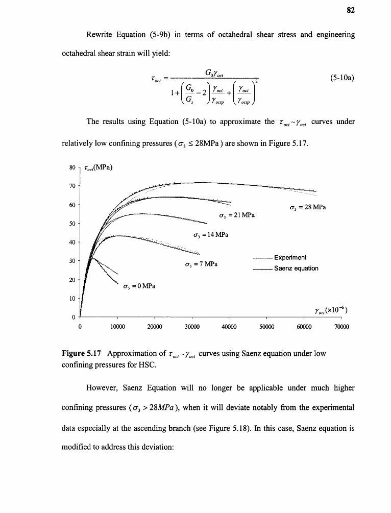
82
Rewrite Equation (5-9b) in terms of octahedral shear stress and engineering
The results using Equation (5-10a) to approximate the r oc, ~ roc, curves under
relatively low confining pressures ( (73 5 28MPa ) are shown in Figure 5.17.
However, Saenz Equation will no longer be applicable under much higher
confining pressures (ay > 28MPa), when it will deviate notably from the experimental
data especially at the ascending branch (see Figure 5.18). In this case, Saenz equation is
modified to address this deviation:

83
Due to the low occurrence probability of very high confining pressures (U y > 60%f) in
practical cases, the Saenz Equation (5-10a) is more appropriate to approximate the true
zocl r yoct relationship of HSC under triaxial compression.
Figure 5.18 Approximation of roc/ ~ roc, curves using modified Saenz equation under
high confining pressures for HSC.
5.3.3.4 Relationship between Peak Octahedral shear stress T Toctpand Peak
Engineering Octahedral shear strain yoctp In order to employ Saenz Equation
(5-10a), the peak secant shear moduli A s of HSC under different stress combinations in
triaxial compression need to be determined. This is to be done by establishing a
relationship between r rocipand Cocoa, as is shown in Table 5.5 and Figure 5.19.

84
Figure 5.19 shows that there is a fairly linear relationship between roc,p and yoetp
which takes a form of:
rood, can be determined by using the failure criterion discussed earlier in this chapter, and
then the Comp can be calculated from Equation (5-11).

85
Until now the only thing which needs to be defined in Equation (5-10a) to finalize
the shape of r ocm ~ rocm curve of HSC in triaxial compression is the initial shear modulus
G0. From the triaxial experiments, the G0 and K0 of HSC under different load paths are
shown in Table 5.6.

86
From table 5.6 it can be seen that although there is a small difference between the
initial shear moduli G0 under different load paths, this variation is trivial compared with
that of the initial bulk moduli Ko. Therefore it is quite reasonable to take an initial shear
modulus G0 of 0.0175x 10 6 MPa for the HSC under such loading cases.
5.4 Equivalent Uniaxial stress ~ strain Relationship
The concept of equivalent uniaxial strss ~ strain relationship was originally put forward
by Darwin and Pecknold (1977) in an attempt to simulate the variation of tangent elastic
modulus Ei with the stress or strain change along the specific axis "i" of the orthotropic
material in biaxial compression. Elwi and Murray (1979) extended this concept to triaxial
compression. The detailed description of the equivalent uniaxial strain 6 . 6 and its
corresponding peak value s be provided later in Chapter 7.
The definitions of the incremental and total equivalent uniaxial strain de,, and
c, are as follows:
where Ei is the tangent elastic modulus in "i" direction under the current stress condition.
It is obvious from Equation (5-12) that debit represents the increment of strain in
direction "i" that concrete would exhibit if subjected to a uniaxial stress increment dais
with other stress increments being equal to be zero. Therefore, if the relationship between
stress a, and equivalent uniaxial strain ch is defined, the variation of the tangent elastic
modulus Ei can be determined.

87
The load path T-1 is especially useful for deriving the equivalent uniaxial stress ~
strain curves under triaxial compression, which can be illustrated by Figure 5.20 and
Table 5.7. In Figure 5.20, a l and 6 3 are first increased proportionately to o and a;
under a constant 63 /6 l ratio of 1/2, and then with a 3 unchanged, o is increased until
the failure strength o- 1 , is reached. However, if the stress ratio was kept the same with the
initial value of 1/2 until failure, o and 6 3 would follow the path of the dash line to a l,
and o-3, respectively. From Equation (5-5), a;, is more than 140 MPa.
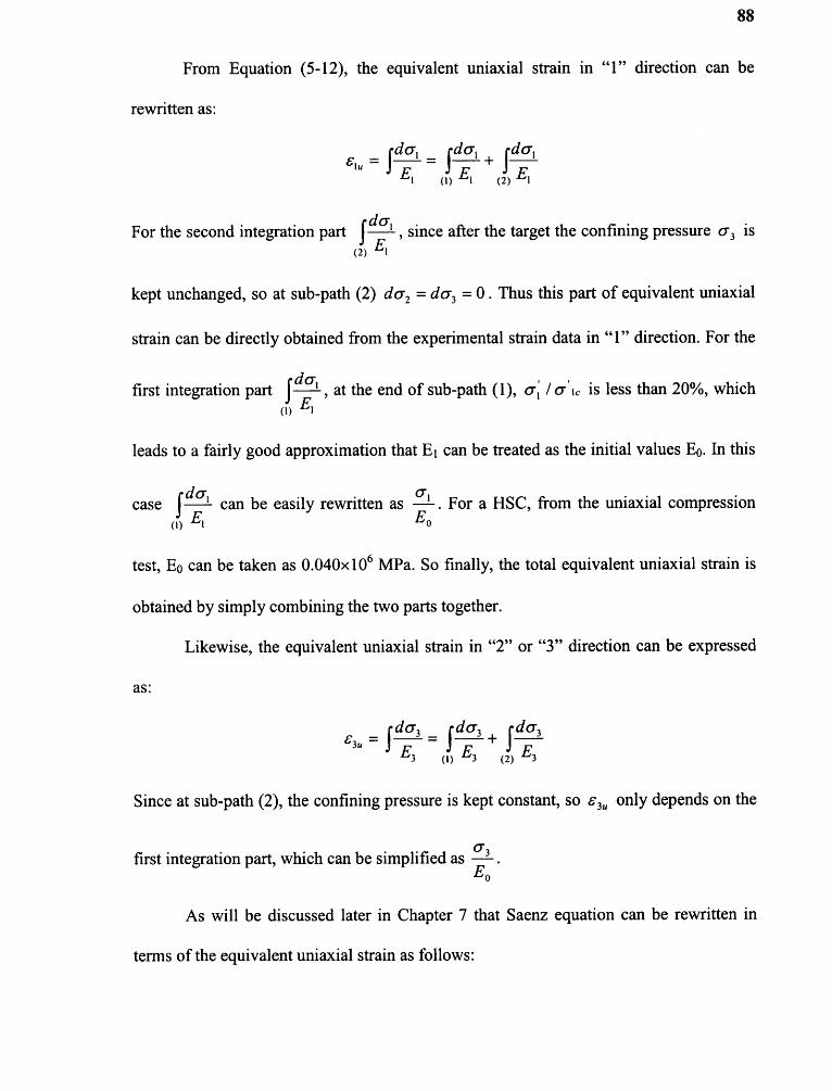
88
From Equation (5-12), the equivalent uniaxial strain in "1" direction can be
rewritten as:
For the second integration part i do-1 , since after the target the confining pressure 6 3 is(2) Ai
kept unchanged, so at sub-path (2) do-2 = do-y = 0 . Thus this part of equivalent uniaxial
strain can be directly obtained from the experimental strain data in "1" direction. For the
first integration part C doe----1 , at the end of sub-path (1), o-, / 6'1 is less than 20%, which(A) EA
leads to a fairly good approximation that E 1 can be treated as the initial values E0. In this
case f do---AI can be easily rewritten as al . For a HSC, from the uniaxial compression
(I) E1 E 0
test, E0 can be taken as 0.040x 10 6 MPa. So finally, the total equivalent uniaxial strain is
obtained by simply combining the two parts together.
Likewise, the equivalent uniaxial strain in "2" or "3" direction can be expressed
as:
Since at sub-path (2), the confining pressure is kept constant, so 8yt only depends on the
first integration part, which can be simplified as --- 2cr .Eon
As will be discussed later in Chapter 7 that Saenz equation can be rewritten in
terms of the equivalent uniaxial strain as follows:
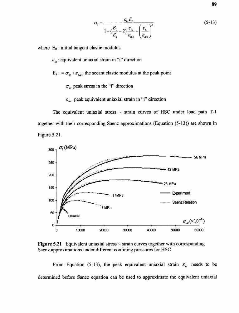
89
where E0 : initial tangent elastic modulus
equivalent uniaxial strain in "i" direction
Es : = a, / e i„, the secant elastic modulus at the peak point
cry„ peak stress in the "i" direction
ei peak equivalent uniaxial strain in "i" direction
The equivalent uniaxial stress ~ strain curves of HSC under load path T-1
together with their corresponding Saenz approximations (Equation (5-13)) are shown in
Figure 5.21 Equivalent uniaxial stress ~ strain curves together with correspondingSaenz approximations under different confining pressures for HSC.
From Equation (5-13), the peak equivalent uniaxial strain e„ needs to be
determined before Sanez equation can be used to approximate the equivalent uniaxial

90
stress ~ strain relationship. Elwi and Murray (1979) assumed that the ultimate (failure)
surface of the equivalent uniaxial strain is analogous to that of the ak and the William-
Warned failure criterion is still applicable by simply replacing fc , 6„, , Q, , 62 and
63 in Equation (5-4) with6ctY gm , elate , 6214C and 6 3 ,4c , respectively, where the * in
the notation represents the equivalent uniaxial quantities. Table 5.8 and Figure 5.22 show
the compressive meridian of the equivalent uniaxial strain c iuc of HSC from this study.
From Figure 5.22, the compressive meridian of the equivalent uniaxial strain
epic takes a form of

91
Figure 5.22 Compressive meridian of the equivalent uniaxial strain for HSC.
5.5 Poisson's Ratio in Triaxial Compression
Some researchers (Chen 1982, Guo 1997 and Zhu 1998) have lamented the dearth of data
on the Poisson's ratio under multiaxial stress conditions. Up until now, almost all of the
available empirical equations about the variation of Poisson's ratio with stress status are
derived from the uniaxial compression tests. Among them, Kuper's equation (Kupfer et.
al 1969) is represented in terms of the ratio of current strain c to the peak value cc.:
Given the initial Vo to be 0.20, the tangent Poisson's ratio at peak will be 1.12.
Based on Ottosen's description, Guo (1997) proposed an equation in terms of the
ratio of current stress i to the peak value ai fl :

92
Both of those two equations are only applicable at the ascending branch of the stress —
strain curve.
Load path T-1 is expedient to derive the tangent Poisson's ratio variation in
triaxial compression status after the target confining pressure is reached, when dcr3 is 0
and consequently am is just equal to de y / de, . This variation with the axial stress ratio
/ cric under different confining pressures is shown in Figure 5.23.
It can be seen from Figure 5.23 that the Poisson's ratio variation of HSC with
stress ratio 13 under different confining pressures are highly changeable. The lower the
confining pressure, the higher the initial tangent Poisson's ratio o . When confining
pressure is 0 (uniaxial compression), a ce, is 0.20 and Carl is 1.12, which well fits with the
prediction of those two empirical equations. However, when confining pressure is as high
as 42 or 14 MPa, o is just around 0.10 and vg. is about 0.6. It seems there is no accurate
way to describe the changing rule of Poisson's ratio of the HSC, which may be attributed
to the erratic non-linear behavior of this material.
As will be discussed later in Chapter 7, in order to maintain a positive definite
stiffness matrix of the constitutive equation, some certain limits were imposed to the
Poisson's ratio by some researchers. Eli and Murray (1979) put a 0.5 limit, but they
only considered the ascending part of the stress ~ strain curve. Also it can be seen from

93
Figure 5.23 this limit of 0.5 is by no means close to the actual scenario that the tangent
Poisson's ratios of HSC at peak under different confining pressures (0 — 42 MPa) are all
around 1.5 or larger than that. For the descending branch, it can be seen from Figure 5.23
that Poisson's ratio is highly unpredictable with a wide range from about 1.5 (high
confining pressures) to 2.5 (low confining pressures), but there seems to be a general
trend that when the confining pressure is higher than 14 MPa, the Poisson's ratio after
peak lingers around 1.0.
Figure 5.23 Poisson's ratio variation of HSC with stress ratio P.
In view of all those aspects, an expression for Poisson's ratio of HSC under
tnaxial compression in terms of stress ratio p (o 1 Bic) is given as follows:

94
Figure 5.24 shows the approximation of the proposed expression to the
experimental results.
Figure 5.24 Proposed Poisson's ratio of HSC under triaxial compression.
The initial tangential Poisson's ratio vo is taken as 0.15, which is appropriate
under moderate confining pressures (3.5MPa ~ 14 MPa), and this value is smaller than
that of the uniaxial compression (Fo =0.2). Up to 50% percent of stress ratio o / aic, the
tangent Poisson's ratio is deemed as a constant, and 1.5 is adopted for vt at the peak. It is
very hard to predict the tangent Poisson's ratio of HSC after peak, which is highly
dependent on the confining pressure. At this stage it is presumably taken as a constant
1.0, which is found to be more appropriate to illustrate the experimental results of most
tests, especially under relatively large confining pressures.
5.6 Cyclic Loading in Triaxial Compression
Cyclic loading was applied after the target confining pressures had been reached for two
confining pressures (14 MPa and 21 MPa). The unloading took the load control mode

95
with the decrease rate of axial stress being 40 MPalmin and the confining pressure being
kept unchanged. After axial stress was reduced to the target value, the control mode was
switched back to the original displacement control again all the way up to the next load
cycle. The testing results are shown in Figure 5.25 and Figure 5.26.
From Figure 25 and Figure 26 it can be clearly seen that a more obvious cyclic
loop in this stress ~ strain curve will be formed if the unloading goes back to a lower
axial stress. Although it does not seem to be very apparent, the slope of each unloading
and reloading portion actually does undergo a notable degradation, as can be found in
Figure 25(a) and 25(c). For instance, under confining pressure of 14 MPa, just after 4
cycles which were separated almost equally by the displacement control, the shear
modulus G lost about 64% (0.0181x10 6 MPa to 0.0066x 10 6 MPa) of its initial value, and

Figure 5.25(b) Octahedral normal stress (sod ~ volume change in cyclic loading underconfining pressure o y =14MPa for HSC.
96

Figure 5.26(a) Axial stress ~ strain curve in cyclic loading under confining pressure6 y=21MPa for HSC.
97
Figure 5.26(b) Octahedral normal stress (Y ou ~ volume change in cyclic loading underconfining pressure 6 y=21MPa for HSC.

98
1.1...INV•
After the comparison between the triaxial stress ~ strain curves of monotonic
loading and cyclic loading under the same confining pressures, it is found that the
envelops of the cyclic loading curves maintain the same shape with those of the
monotonic loading.
5.7 strains during Cyclic Loading
The relationship between the lateral strain Ey and axial strain El for HSC during cyclic
loading is shown in Figure 5.27.
It seems that the strain development during cyclic loading does not deviate much
from the mainstream of that under monotonic loading. Since during cyclic loading the
confining pressure maintains the same, it is quite reasonable to assume that the Poisson's
ratio of HSC during cyclic loading takes the same tangent value at the point where the
unloading occurs.

Figure 5.27 Lateral strain sy ~ axial strain Cl during cyclic loading under confiningpressure a y=14MPa for HSC.
99

CHAPTER 6
TRIAXIAL COMPREssION TEsT REsULTs OF STEEL FIBER REINFORCEDHIGH sTRENGTH CONCRETE (sFHsC)
6.1 Experimental Program
The raw materials and mix proportion of the SFHSC are essentially the same with those
of the HSC listed in Table 5-1 except for the additional introduction of 1% volume ratio
of hook ended 30mm long steel fiber with a diameter of 0.5 mm. Compared with the
SFHSC in Chapter 3, due to the change of aggregates, the standard compressive strength
f: is down from 79.5 MPa to 14.3 MPa and initial elastic modulus E0 is down from
48800 MPa to 41400 MPa.
100mmx200mm (4x6 in.) concrete cylinders with both ends ground under
designed lubricated loading platen were mainly used in this part. However, to make
comparison, several tests using regular 100mmx200mm (4x8 in.) cylinders under
standard rigid loading platen were also performed to study the difference between those
two situations in terms of triaxial strength and triaxial stress ~ strain behavior.
In this part, three different load paths were adopted, namely T-2, T-3 and T-4.
There is also another load path T-2' which is just a derivative of load path T-2 and aimed
100

101
at coping with high confining pressures which cannot be reached simply by the
application of T-2. Those three load paths are shown in Figure 6.1.
Figure 6.1 Different load paths used in triaxial compression of SFHSC.(6, -axial stress, a y -confining pressure)
Load control was employed before the target confining pressure a 3 was reached
with the increasing rate of 6 3 being 7 MPalmin. After the target 6 3 , displacement
control was adopted all the way up to the failure (including strain softening) of the
specimen. The displacement rate was controlled within a range from 0.005 mm/s (0.0002
finks) to 0.010mm/s (0.0004 in/s).
6.2 Failure Criterion
6.2.1 Mohr-Coulomb Failure Criterion
The triaxial compression test results of the SFHSC concerning the Mohr-Coulomb failure
criterion are listed in Table 6.2 and Figure 6.2.

Table 6.2 Triaxial Strength of SFHSC for Mohr-Coulomb Failure Criterion
102
Figure 6.2 Mohr-Coulomb failure criterion of SFHSC.

103
From Figure 6.2 it is shown that the Mohr-Coulomb failure criterion of SFHSC
can be expressed as:
Compared with that of the HSC (Equation (5-3)) in which k is equal to 4.0, those
two equation are essentially the same. From Equation (5-2), it is indicated that the
introduction of the steel fibers does not influence the internal friction angle 0 of the
HSC.
6.2.2 Willam-Warnke Failure Criterion
The experimental results for establishing the Willam-Warnke failure criterion are listed in
Table 6.3, and the compressive meridian is shown in Figure 6.3.
Table 6.3 Triaxial Strength of SFHSC for Willam-Warnke Failure Criterion

104
Figure 6.3 indicates that regardless of the different load paths and specimen sizes,
there is a good correlation between am / fc and T . / f: . The compressive meridian of the
SFHSC can be expressed as
The compressive meridian for the HSC is defined in Chapter 5 as
Figure 6.3 Compressive meridian of Willam -Warned failure criterion for SFHSC.
Figure 6.4 shows the data points of the compressive meridians for both HSC and
SFHSC. It can be found that the difference between them is really trivial, so a uniform
compressive meridian can be adopted for both of the concretes.

105
Figure 6.4 Comparison of compressive meridians of HSC and SFHSC.
In the previous section, it has been found that the introduction of steel fiber does
not affect the Mohr-Coulomb failure criterion (k and internal friction angle 0 ) in triaxial
compression. Combined with what has been found in this section, it seems that the
introduction of steel fiber makes no difference for HSC under triaxial compression in
terms of ultimate surface of stress.
Figure 6.5 shows the comparison of the compressive meridians of the SFHSC
from this study and some previous researches (Ahern 1992 and Ishikawa et al 2000). The
testing results of Chern (1992) were from the steel fiber reinforced normal strength
concrete (f:: 125MPa ), while those of Ishikawa et al (2000) were obtained from the
fiber reinforced concrete which had the same strength grade with this study. All of the
experimental data essentially follow the same trend except for that the Ishikawa's data
have relatively lower upper bound of an,/ f:.

106
Figure 6.5 Comparison of compressive meridians of SFHSC for this study and resultsfrom Ishikawa et al (2000) and Chem (1992).
6.3 Triaxial stress ~ strain Relationship
6.3.1 strains at Peak stress under Triaxial Compression
Table 6.4 shows the peak lateral strain 6yc and peak axial strain e l , of SFHSC under
different load paths and confining pressures.
From Table 6.4 it seems that different load paths do not have a substantial
influence on the peak lateral strain 8yc and the peak axial strain e l,. Under the confining
pressure of 28 MPa, the cylinders under load paths T-2, T-3 and T-4 almost have the
same ey, and el . The only exception occurs under load path T-2', where the peak
lateral strain 6yc is quite abnormal and even larger than the value under a confining
pressure of 42 MPa. This was later found out to be the fallout of a highly non-uniform
lateral expansion of the cylinder under that load path.

107
* abnormal
Table 6.5 compares the peak lateral strain sac and peak axial strain e l, of SFHSC
with those of HSC under certain confining pressures. It indicates that under triaxial
compression, the introduction of the steel fibers into the HSC does not provide the
obvious advantage in terms of the peak lateral strain e3c and peak axial strain which
means the deformation capacity of SFHSC before failure does not have a noticeable
improvement compared with HSC under triaxial compression.

Table 6.5 Comparison of e y, and E l, between HSC and SFHSC
108

109
Compared with Equation (5-6a), this expression is a little bit different in that the
constant "17.33" is a little lower. However, it should be noted that this difference is
caused by the additional two more points ( a y =63 MPa and 14 MPa). Were those points
ignored, Equation (6-3a) would be almost same with Equation (5-6a).
Like HSC, a good relationship between the lateral peak strain 6 yc and axial peak
strain 6 1 , under different confining pressures is shown in Figure 6.7, which can be
expressed as follows:
Figure 6.7 Relationship between axial and lateral strains at peak for SFHSC undertriaxial compression.

110
6.3.2 Axial stress versus strains under Various Confining Pressures
Under load path T-2 (T-2' for confining pressure 42MPa, 14MPa and 70MPG), the axial
stress ~ strain (axial and lateral) curves of SFHSC are shown in Figure 6.8. The load path
T-2' for confining pressure 28MPa, 42MPa, 14MPa and 14MPa is defined in Figure 6.9.
It should be noted that T-2' was just modified from T-2 in order to reach high confining
pressure before the failure of the specimens.
The load paths T-2 and T-2' are designed to maintain a lateral expansion of the
specimen under triaxial compression since the increment of confining pressure a 3 is
much smaller than that of the axial stress a l , which is good for a more accurate lateral
strain measurement (it has been found that the circumferential extensometer is more
sensitive in detecting expansion than contraction since it is only driven by two springs).
Thus in Figure 6.8, the lateral strains sy are all in expansion (negative side).
Compared with the triaxial stress ~ strain curves of HSC (load path T-1) as shown
in Figure 5-9, the shape of the triaxial stress ~ strain curve of SFHSC undergoes some
variation under high confining pressures (14MPa, 70MPa). In those two cases, before the
target confining pressure is reached, the curves can be approximated by two straight lines
(see Figure 6.8).

111
Figure 6.8 Axial stress versus strain curves of SFHSC at different confining pressures(Load path T-2).
Figure 6.9 Load path T-2' under different confining pressures O.
The triaxial stress ~ strain curves of SFHSC under different load paths for
confining pressure 0-y =28 MPa are shown in Figure 6.10. For load path T-4 (Figure 6.1),
the specimen was first applied to an axial stress of 42 MPa (60% f; ).

Figure 6.10 Axial stress versus strain curves of SFHSC under different load paths atay = 28MPa .
It can be seen from Figure 6.10 that the four axial stress — axial strain curves
follow the same trend except that T-3 and T-4 are somehow steeper than T-2 and T-2'
under high axial stresses. This is understandable since around that region the confining
pressures for T-3 and T-4 is relatively higher than those of T-2 and T-2'.
6.3.3 Octahedral stress~strain Relationship
6.3.3.1 Octahedral Normal stress versus Volume Change The Octahedral normal
stress versus volume change of SFHSC under load path T-2 at different confining
pressures (0 ~ 14 MPa) is shown in Figure 6.11. Like HSC (Figure 5.11), the initial

113
of the confining pressure, the tangent bulk moduli tend to become larger. As can be seen
from Figure 6.11, the curves under higher confining pressures become steeper with the
increase of (• rocm .
Figure 6.11 o-ocm versus volume change of SFHSC at different confining pressures(load path T-2).
Figure 6.11 also shows that SFHSC starts to reverse from contraction to dilation
just right before the peak stress is reached, which complies with Gerstie's description
(Gerstle 1981) for normal strength concrete. At that turnaround point, the stress ratio
croc aoct is around 95%. Similar to the uniaxial test result, the bulk modulus, which is
The effect of the load path on the volume change of SFHSC under the same
confining pressure is shown in Figure 6.12. Like HSC (Figure 5-12), there are some
differences between the maximum contractions of SFHSC under triaxial compression,
but the variation trends are almost the same.

114
Figure 6.12 co, versus volume change of SFHSC under different load paths at
63 = 28MPa
6.3.3.2 Octahedral shear stress r oc, ~ Engineering Octahedral shear strain r.„
As will be discussed later in Chapter 7, 'rod ~ roc, curve under triaxial compression is of
great importance to establish a constitutive model for both HSC and SFHSC and is the
key to this study.
Figure 6.13 depicts the "rod ~ rod curves of SFHSC for different confining
pressures under load path T-2 and T-2'. Under high confining pressures (14MPa and
70MPa), like the axial stress ` strain relationship (Figure 6.8), the root ~ rod curves also
deviate from the typical parabolic shapes and manifest some kind of bilinear
characteristic before the target confining pressures.
Figure 6.14 illustrates the normalized version of Figure 6.13. It can be found that
upon normalized, there is clearly a general trend for all T oil ~ r oct curves except that the

115
slope of the uniaxial one before peak is steeper than the triaxial ones. The post peak
deviation from the mainstream for roci — y,,,, curve under the confining pressure of 14MPa
may be attributed to experimental errors.

116
Figure 6.20 shows the rod ~ y„,m curves of SFHSC under different load paths for
the confining pressure of 28MPa. Since they are essentially following the same trend, it
should be appropriate to use a uniform expression to approximate all of them.

117
Figure 6.16 demonstrates that the experimental roc,— focm curves comply with the
Saenz equation fairly well under moderate confining pressures ( a y __ 28MPa ). However,
under high ay (42MPa, 14MPa, and 7OMPa), the experimental 1- FOCI ~ foci curves are far
below the Saenz prediction. In this case, a modified Saenz equation like Equation (5-10b)
can be adopted (see Chapter 5 and Chapter 7).

118
Toctp and was studied for SFHSC under different load paths and confining pressures,
and the results are shown in Table 6.6 and Figure 6.17, respectively.

119
From Table 6.6 and Figure 6.17, the relationship between rod and y„,mp of
SFHSC can be written as:
It is quite close to the same equation of HSC, which is expressed as:
If those two groups of data (HSC and SFHSC) are plotted on the same graph
(Figure 6.18), it is quite clear that all the data can be expressed by a single expression,
either Equation (5-11) or Equation (6-5). There is really not much difference between
SFHSC and HSC in terms of the peak octahedral shear stress and strain.

120
6.4 Equivalent Uniaxial stress ~ strain Relationship
The detailed description on deriving the equivalent uniaxial strain has been given in
section 5.4 of Chapter 5, and is hereby abridged. The calculation was based on load path
T-2 ( ay =7MPa and 14MPa) and T-3 ( a y =28MPa). Results for SFHSC are shown in
Table 6.7, Table 6.8, Figure 6.19 and Figure 6.20, respectively.

121
Figure 6.19 Compressive meridian of equivalent uniaxial strain Ai., of SFHSC andHSC under triaxial compression.
All the data from both SFHSC and HSC for the compressive meridian of the
equivalent uniaxial strain are shown in Figure 6.19, which can be summarized into a
regression equation of which R2 is equal 1.0:

122
Figure 6.20 Equivalent uniaxial stress~strain curves and Saenz approximation ofSFHSC under different confining pressures.
6.5 Comparison of stress ~ strain behavior of Different specimen sizes under
Triaxial Compression
In this research, the 100mmx 200mm (4"x6") cylinders together with designed lubricated
loading platen are mainly used to study the triaxial compression behavior of SFHSC. It is
necessary to make a comparison with the commonly used testing method in which
standard 100mmx200mm (4"x8") cylinders and rigid loading platens are employed.
Under the same load path T-2 in triaxial compression, it has been found from Table 6.2
and 6-3 that those two methods make no noticeable difference in terms of triaxial strength
and failure criterion. Also Table 6.4 shows that the peak strain values (A l, and Ely,) for
both two cases are close to each other.
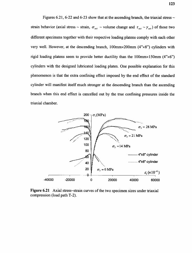
123
Figures 6.21, 6-22 and 6-23 show that at the ascending branch, the triaxial stress
strain behavior (axial stress ~ strain, crocr ~ volume change and rod-rod ) of those two
different specimens together with their respective loading platens comply with each other
very well. However, at the descending branch, 100mmx200mm (4"x8") cylinders with
rigid loading platens seem to provide better ductility than the 100mmx 200mm (4"x6")
cylinders with the designed lubricated loading platen. One possible explanation for this
phenomenon is that the extra confining effect imposed by the end effect of the standard
cylinder will manifest itself much stronger at the descending branch than the ascending
branch when this end effect is cancelled out by the true confining pressures inside the
triaxial chamber.
Figure 6.21 Axial stress~strain curves of the two specimen sizes under triaxialcompression (load path T-2).
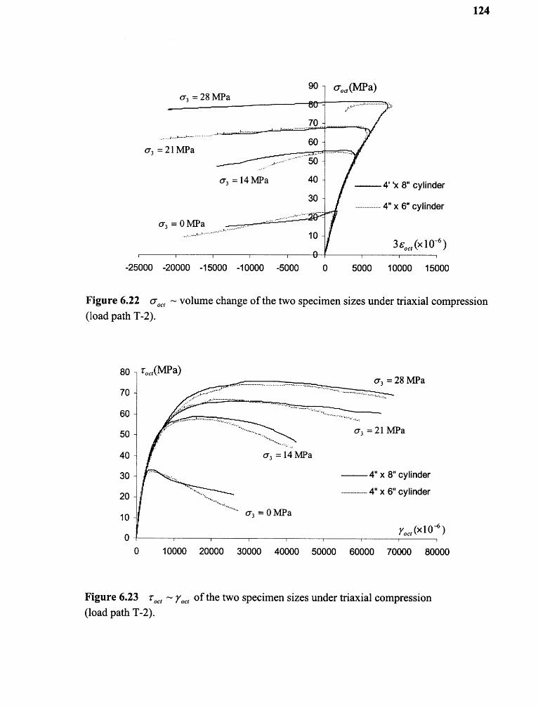
124
Figure 6.22 o-oc ~ volume change of the two specimen sizes under triaxial compression(load path T-2).

125
6.6 Poisson's Ratio in Triaxial Compression
The tangent Poisson's ratio of SFHSC under triaxial compression is shown in Figure
6.24. In this part of experiment only two cases, namely confining pressure 28MPa under
load path T-3 and confining pressure 7MPa under load path T-2 are suitable for
evaluating this variation. It is found that the tangent Poisson's ratio after peak Bo, takes a
constant value from 0.9 to 1.2 for these two cases.
Figure 6.24 Variation of tangent Poisson's ratio of SFHSC with stress ratio undertriaxial compression.
It can be seen from Figure 6.24 that the variation of t with stress condition for
HSC (Equation 5-17) can also be applied to SFHSC under triaxial compression. Thus, a
uniform expression can be developed for both of them.
6.7 Triaxial stress ~ strain Behavior under Cyclic Loading in Triaxial Compression
Like HSC, the load control mode was used in the unloading path with the decrease rate of
axial stress being 40 MPa/min and the confining pressure being kept unchanged. After

126
axial stress was released to the target value, the control mode was switched back to the
original displacement control again all the way up to the next load cycle.
The typical cyclic loading behavior is shown in Figure 6.25 (a) (b) and (c) for the
load path T-3 and the confining pressure of 28 MPa. The other cases are shown in the
appendix A. Like HSC, SFHSC also experienced appreciable degradation in terms of the
elastic modulus E (Figure 6-25(a)) and shear modulus G (Figure 6-25(c)) under cyclic
loading, and there seems no good way to simulate this degradation trend. However, the
cyclic loading does not change the general envelop of the triaxial stress ~ strain curves of
SFHSC.

127
6.8 strains During Cyclic Loading
The typical relationship of lateral strain cy versus axial strain c of SFHSC during cyclic
loading is shown in Figure 6.26. The confining pressure is 28 MPa under load path T-3.
For the other cases, the results are shown in Appendix B.
It can be seen from Figure 6.26 that, like HSC, the variation of those two strains
under cyclic loading does not deviates too much from the mainstream relationship, and it
may be applicable to take a constant tangent Poisson's ratio for a single unloading and
reloading process, which is equal to the value right at the unloading point.

Figure 6-26 Axial strain El ~ lateral strain cy of SFHSC during cyclic loading underconfining pressure 6y=28MPa (load path T-3).
128

CHAPTER 7
AN INCREMENTAL CONsTITUTIVE MODEL FOR HsC AND sFHsC UNDERTRIAXIAL COMPREssION
7.1 Introduction of Orthotropic Incremental Constitutive Models
7.1.1 Darwin-Pecknold Constitutive Model — 2D
Darwin and Pecknold (1977) proposed a constitutive stress ~ strain relationship to model
the general biaxial loading histories (including cyclic loading). This model is supposed to
be used in conjunction with the finite element analysis, so an incremental (tangent) rather
than total (secant) form has been adopted. In this model, the concrete is treated as an
incrementally linear elastic material, and at the end of each stress or strain increment, the
material properties, essentially E (elastic modulus) and F (Poisson's ratio), are adjusted to
reflect the latest changes in deflection (strain) or load (stress).
If the shear stress is neglected and only the principal stress axes are considered,
the incremental stress ~ strain relationship can be described as the following:
where E1 : tangent elastic modulus in the "i" direction
F1 : tangent Poisson's ratio induced by the stress in "i" direction
Equation (7-1) can be reqritten into another form:
129

130
The constitutive matrix in Equation (7-2a) will be totally defined once E1, E2 and
F are given. Those three variables will be determined by using an initiative concept —
equivalent uniaxial strain, s at, .
The concept of "equivalent uniaxial strain" was originally developed by Darwin
and Pecknold to duplicate the actual biaxial stress ~ strain curves directly from the
uniaxial counterpart and then use it to simulate the variation of elastic modulus and
Poisson's ratio under different stress conditions. This concept can be better illustrated if
one reshuffles the Equation (7-2a) to Equation (7-2b):
where cleit is the "equivalent uniaxial strain" increment. Comparing it with the original
equation, one can easily achieve
The incremental equivalent uniaxial strain Nei., which can be either positive or
negative, may be defined more explicitly from Equation (7-2b) as
The physical meaning of Neat is clearly demonstrated from the last equation as the
increment of strain in the "i" direction that concrete would experience if subjected to a
uniaxial stress increment Napa with other stress increment equal to zero. For a nonlinear

131
material like concrete, equivalent uniaxial strain eh, represents the portion of strain in the
"i" direction eliminating Poisson's effect that controls the material behavior such as
softening and failure. It should be noted that the equivalent uniaxial strain is a fictitious
material index which is invented to simplify the procedures to attain the other true
parameters such as elastic modulus E1 and Poisson's ratio v.
Uniaxial stress ~ strain curve proposed by Saenz (shown in Equation (7-3)) was
adopted in this constitutive model by replacing the uniaxial strain e, with corresponding
equivalent uniaxial strain Eh :
where E0 : initial tangent elastic modulus
Differentiating both sides of Equation (7-3) with respect to equivalent uniaxial
strain e yield the tangent elastic modulus E1:

132
normal strength concrete under proportional loading has been thoroughly studied by
many researchers. Kupfer and Gerstle (1973) have suggested an analytical maximum
strength envelop for biaxial loading as shown in Figure 7.1.
Figure 7.1 Biaxial strength envelop by Kupfer and Gerstle (1973).
Complying with this envelop, Kupfer and Gerstle also proposed simplified
expressions of biaxial strength for different stress combinations. For compression-
compression, the o is approximated by

133
For tension-compression, Kupfer and Gerrstle adopted a linear reduction of tensile
strength in accordance with the increased compression:
For tension-tension, a constant biaxial tensile strength equal to the uniaxial tensile
strength f was recommended.
Compared with a-k , determining e jet, is highly empirical and hypothetical. The
following equation is used:
in which e. is the peak strain for the uniaxial compression and
e jet, (a = 1) can be calculated from the actual peak strain assuming a constant Poisson's
ratio equal to 0.2. It is indicated that R is approximately 3 from the available data.
However, Equation (7-9) does not fit well for a!, which is less than f: . In this
case east, is taken as:
134
Based on the uniaxial and biaxial experimental results from Kupfer, Hilsdorf, and Rusch
(1973), Darwin and Pecknold (1977) proposed that the so-called "effective" Poisson's
ratio v , which is equal toT/ 2 , would be defined correspondingly in different stress
combination domains: for tension-tension and compression-compression v = 0.2 ; for
uniaxial compression and tension-compression,
where a l and a 2 represent compression and tension components, and f and f, stand
for the uniaxial compressive and tensile strength of the concrete, respectively. For
uniaxial tension, concrete is assumed to be a linear elastic material with v = 0.2 .
Right now all the unknown parameters in Equation (7-2a) have been determined.
As the load is applied, the equivalent uniaxial strain is calculated, accumulated and
then entered into Equation (7-4) to determine the current tangent moduli El and E2.
This model is relatively simple and the parameters can be calibrated from the
uniaxial stress ~ strain curve and numerous reported biaxial experimental studies.
However, it is only applicable to the planar problems and cannot account for the 3-D
situations. Moreover, during the construction of the equivalent uniaxial stress— strain
curve, it assumes a constant Poisson's ratio value of 0.2, which is contradictory to the fact
that this ratio will deviate progressively after about 60% of the peak stress. And what's
more important, due to the lack of experimental data at the descending branch of the
stress ~ strain curve, this model can only simulate the behavior of concrete at the
ascending part under biaxial loading.

135
7.1.2 3D Incremental Concrete Constitutive Relationship
Elwi and Murray (1979) extended the usage of the orthotropic incremental constitutive
model to the 3D domain. This model is arranged to be expressed in an explicit
formulation which can be readily incorporated into the finite element analysis, applicable
in the cyclic loading and determined completely by the conventional parameters such as
uniaxial compressive strength f: , uniaxial tensile strength f, , uniaxial crushing strain
e and initial elastic modulus E0. Like the Darwin-Pecknold 2D model, the concept of
equivalent uniaxial strain is also introduced in this model and becomes the basis upon
which the incremental elastic moduli and Poisson's ratios are derived in terms of strain
parameters.
7.1.2.1 Form of Incremental Constitutive Relation This 3D model initially is
intended for use in the axisymmetrical structures. If orthotropy is assumed, the
incremental stress—strain constitutive matrix can be written as a 4x4 matix when referred
to the orthotropic principal axes:
where Ei represents the elastic modulus in the axis of orthotropy "i" and Cy represents the
possion's effect of strain occurring in the "i" direction induced by the stress in the "j"
direction. G is the shear modulus.
If symmetry is assumed in the constitutive matrix of Equation (7-12), then:

Substituting those constraints into Equation (7-12) and rewriting it yield
136

137
required to be determined. Herein the concept of equivalent uniaxial strain is introduced.
The technique is described as follows.
Arbitrarily rewrite Bquation (7-14) as
Then the incremental and total equivalent uniaxial strain Ne„ and salt can be evaluated
from
Again, NEB, represents the increment of strain in direction "i" that concrete would
exhibit if subjected to a uniaxial stress increment No-, with other stress increments equal
to be zero. It depends on the current stress condition and belongs to a fictitious parameter
that is only significant as a base to evaluate the variation of other material indices, like
elastic modulus and Poisson's ratio.

138
7.1.2.2 Equivalent Uniaxial stress ~ strain Curve In this model, a modified Saenz
uniaxial compressive stress ~ strain relationship which incorporates the description of the
descending branch and can be used to simulate both the tensile and compressive
responses of concrete is adopted. The equation is written in terms of equivalent uniaxial
strain as
In Equation (7-18), B0 represents the initial tangent elastic modulus; a ►, is the
maximum stress in the "i" direction that occurs for the current particular principal stress
ratio, and represents the corresponding equivalent uniaxial strain; (o-v , eve) is a
selected point on the descending part of the equivalent uniaxial stress ~ strain curve. Due
to the high volatility of the descending branch of the uniaxial stress ~ strain curve, Blwi
and Murray recommended an alternative from the flexural behavior of concrete, which
gives

139
Now Equation (7-18) is to be used to derive the incremental elastic moduli Ei in Equation
7.1.2.3 Poisson's Ratio In this model, Poisson's ratio is determined by the uniaxial
compression data of Kupfer, Hilsdorf and Rusch (1969), which is expressed as
where e is the uniaxial strain, e,,, is the uniaxial peak strain and o is the initial
Poisson's ratio.
In this model, it is assumed that the Poisson's ratio C u in Bquation (7-20) is only
the function of the strain or stress in the "j" direction, which will yield only independent
Poisson's ratios:
By replacing those two uniaxial values e and e cuwith corresponding equivalent
uniaxial strains, Elwi and Murray assumed that the three independent Poisson's ratio
C a (i=1,2,3) can also be postulated as follows:

and the equivalent Poisson's ratio ,u„ in Equation (7-20) can be written as
In this model, the variable 4 in Equation (7-20) is set to be a non-negative value.
Therefore a limiting value of 0.5, which corresponds to a limit of zero incremental
volume change, has been placed on the Poisson's ratio C i determined by Equation (7-21).
Elwi and Murray insisted that placing this limit would yield realistic estimates of stress.
However, it has been shown in the octahedral normal stress (c r 0,,) versus volume change
(3E0,, ) curves of the uniaxial and triaxial compression in the former chapters of this
thesis that this zero incremental volume change occurs only at approximately 93%-95%
of the maximum stress. For an instance at the peak stress of the uniaxial compression, the
tangent incremental Poisson's ratio can be as large as 1.0, and after that point it has a
tendency even to keep increasing a little bit on the descending branch of the stress —
strain curve. Therefore, the variable 4 may not always be a non-negative number as it is
postulated to be.
7.1.2.4 Ultimate Surface The surface in the 3D stress space that defines the ultimate
strengths a„ for any combination of stress conditions is called the ultimate surface. In
this model, the Willam-Warnke 5-parameter ultimate surface is adopted to determine the
maximum a, in Equation (7-18) and (7-19). As discussed in the previous sections, the
140

141
tensile meridian and compressive meridian stipulated in this failure criterion can be
expressed as follows:
On the deviatoric plane, three identical parts of an ellipse are used to connect
those points on the meridians:
The determination of the coefficient ao, al, a2, b0, b1 and b2 has been already fully covered
previously.
However, Equations (7-18) and (7-19) also require the evaluation of peak
equivalent uniaxial strains A im,, . So in this model, it is assumed that the ultimate surface of
the equivalent uniaxial strain is analogous to that of the ai and the Willam-Warnke

notation represents the equivalent uniaxial quantities. As can be clearly seen from its
definition, equivalent uniaxial strains eii are fictitious values that cannot be directly
observed except for those corresponding to the uniaxial tension and compression, which
means at least three different fictitious points are needed in order to determine the final
shape of the ultimate surface of the equivalent uniaxial strain. Elwi and Murray did not
provide a detailed procedure on how to get those new points, but instead they just put
forward a very vague description like "These points, have been determined, herein, by
trial and error until reasonable strain correspondence was obtained".
7.1.2.5 Implementation of the Constitutive Model The pivotal part of the model
implementation is to determine the elastic modulus using Equation (7-19). The
procedures can be summarized as follows:
1) Determine the shape of the ultimate surface of peak stresses a, in the stress space and
that of the peak equivalent uniaxial strains chic in the fictitious equivalent uniaxial strain
space;
2) Input the initial elastic modulus E, = E0 and initial Poisson's ratio v i.-- vo ;
3) Input the initial strain increment ddei, use Equation (7-17a) to calculate the equivalent
uniaxial strain Ne,. and c,u , use Equation (7-14) to calculate Nail and 6 ;
4) Find a, by extending a line from the origin point of the stress space through the
current stress point 6 until it penetrates the ultimate surface of peak stresses;

143
5) Find E se by extending a line from the origin point of the equivalent uniaxial strain
space through the current strain point a until it penetrates the ultimate surface of peak
equivalent uniaxial strain;
6) Construct the constitutive matrix [C] of Equation (7-20) again by evaluating tangent
elastic modulus E1 from Equation (19) and Poisson's ratio v a from Equation (7-20);
7) Go back to procedure 3 and continue to input new strain increment Neap .
It can be clearly seen from the above-mentioned procedures that the model
implementation depends on the initial stiffness of each stress increment. Also the
proportional loading case is assumed.
7.2 Evaluation on Previous Incremental Models
7.2.1 Theoretical Limitation of Elwi's Model on Load Path and Poisson's Ratio
In Equation (7-12), it is assumed that the matrix is symmetrical, which will inevitably
lead to:
This argument is probably true under two circumstances: First, when the stress status is
lower than a certain level under which the concrete behaves like a linear elastic material
in all principal directions so that the elastic moduli and Poisson's ratios in all directions
are approximately equal to E0 and v on ; the other case is in the proportional loading where
all principal stresses increase proportionately with respect to one another until failure:

144
Although the elastic modulus and Poisson's ratio are mostly expressed in terms of strain
in Equation (7-19) and (7-21)), clearly they are also functions of stress ratios
:fore, under a proportional loading, the elastic moduli and Poisson's ratios in
all principal directions are kept the same all the time, which will guarantee the symmetry
of the stiffness matrix.
However, that assumption may not be right under non-proportional loading cases.
For instance, just like the triaxial compression loading path shown in Figure 7.2, if the
slope a2 is larger than a A , then near the failure point aday
— < — . Since the tangentalesa3c
elastic modulus decreases while Poisson's ratio increases with the increasing of the stress
ratio —Hai, it will lead to EA > Ey and vAy > vyA, so obviously the equilibriums in Equationcrick
(7-12a) will not be satisfied any more.
Figure 7.2 A non-proportional loading case.

145
However, as Guo (1997) stated, statistically, proportional loading is the most
probable loading case in the real situations, so this assumption does have a wide
applicability.
The 4 value in Equation (7-20) is set to be non-negative, which will inevitably put
an upper limit of 0.5 to all the Poisson's ratios v i . This treatment probably intends to
maintain the stiffness matrix [C] in Equation (7-20) to be positive definite for the sake of
the stability of finite element solutions. But this limit is clearly at odds with the
experimental observations from this research and other studies which show that the
tangent Poisson's ratio of concrete near the peak is well around 1.0.
Bathe (1979) also addressed the issue of stiffness matrix indefiniteness. In his
model, a constant Poisson's ratio was adopted throughout the whole loading process,
including ascending and descending portions of the stress — strain curve, whereas the
tangent elastic moduli E1 can be negative on the descending branch. Therefore, if the
negative elastic moduli are introduced into the stiffness matrix, the stiffness matrix may
become indefinite and the element assemblage stiffness matrix may not be positive
definite, which will result in relatively large errors to the solution of finite element
equations. To circumvent this dilemma, a zero value (actually a small positive value) for
E1 is employed for stiffness calculations, however the real negative Ei is used in stress
calculations. This strategy, as stated by Bathe, is a direct generalization of the common
incremental procedures employed to analyze perfectly-plastic conditions and conditions
of complete stress release.
7.2.2 some Discussion on Positive Definiteness of stiffness Matrix [C]
Consider the stiffness matrix in Equation (7-20)

146
The necessary and sufficient condition for [C] to be a positive definite matrix is
that the determinants associated with all its upper-left submatrices, det(0 3 ) , are all
positive.
to be satisfied, the following restrictions should be met:
1) The tangent Poisson's ratio v i should be less than 0.5 before crick, but after this peak on

147
2) The tangent elastic modulus E. is positive before multiaxial peak stress Bic, and after
that point it can take a negative value, representing the descending branch of multiaxial
stress~strain curve. However, VE; Ei (i#j and i, j=1,2,3) should be always a positive
value, which indicates that i reaches its respective crib,simultaneously for all directions
(i=1,2,3), an apparent outcome of the proportional loading;
3) According to Equations (7-20b) and (7-24d), G12 should always be a positive value.
The extension of the technique to the general three-dimensional situation is
simple, since this only requires the definition of the additional incremental shear moduli
G2y and Gy1 that can be determined in the same manner as G12 (Equation 7-20b).
7.2.3 Evaluation on the Equivalent Uniaxial Strain
The key to the previous incremental constitutive models is to obtain the variation of
tangent elastic modulus E1 through the whole load ~ deformation process. Equation (7-4)
was used in Darwin and Pecknold's model while Elwi's model adopted Equation (7-19)
which is just a modification of Equation (7-4).
It can be seen from Equation (7-4) that in order to have the variation of Ei, the
equivalent uniaxial strain sib, and the peak equivalent uniaxial strain must be input.
Although has been defined by Equation (7-17a), c hi, still remains a problem. As
discussed before, Eli (1979) just assumed that the ultimate surface of the equivalent

148
uniaxial strain took the same format and shape as those of the ultimate stress surface by
replacing the stress parameters in Equation (7-22) with the corresponding equivalent
uniaxial strain ones. He did not describe clearly on how to derive this ultimate surface,
but he did list the results for the normal strength concrete from Kupfer and Schickert-
Winkler. Those two data together with the experimental results from this study (HSC and
SFHSC) are shown in Figure 7.3.
Figure 7.3 Comparison of the compressive meridians of equivalent uniaxial strain fromKupfer, Schickert-Winkler and this study.
Remarkable difference can be found from Figure 7.3. From the computer model
analysis following the model implementation procedures listed above, it has been found
that the ultimate surface of the equivalent uniaxial strain is highly unreliable to be used to
predict the stress ~ strain behavior of HSC under triaxial compression. In this study, this
ultimate surface was obtained by adopting load path T-1, and if it is used to check the
load path T-2, there is a large difference between the prediction and the actual stress

149
strain behavior. Sometimes the computational results do not make any sense. Therefore,
unlike the ultimate surface of the stress which is independent of the load path, the
ultimate surface of the equivalent uniaxial strain seems to have no fixed expression and
the load path seems to have a substantial effect on its shape.
From the model analysis results, another important job that can not be
implemented by the ultimate surface of the equivalent uniaxial strain is the
synchronization of the stress criband equivalent uniaxial strain Aiucto their corresponding
peak values a is and A. From Equation (7-4) it can be easily understood that if the
triaxial stress — strain behavior around peak is to be well predicted, i and eii should get
to their respective ultimate surface ( a k and eiuc) simultaneously in order to get a zero
tangent elastic modulus right at the peak. Since this assumed ultimate surface of the
equivalent uniaxial strain does not truly reflect the deformation behavior of the HSC,
there is no wonder why the equivalent uniaxial strain always precedes or lag behind stress
development greatly, which in turn results in the considerable difference between the
prediction and experimental results.
7.3 A simple 3D Incremental Model for Proportional Loading under TriaxialCompression for HsC and sFHsC
7.3.1 Tangent Elastic Modulus E1
As discussed above, Equation (7-4) is not practical to evaluate the variation of the tangent
elastic modulus Ei since it is based on the fictitious parameters which is hard to
determine and also dependent on the load path. Thus in this model, the concept of the

150
equivalent uniaxial strain is disregarded. Consequently, a more direct and accurate way to
simulate the variation of the Ei needs to be developed.
This new approach comes from the similarity between the equivalent uniaxial
stress ~ strain curve and the octahedral shear stress T ac, ~ octahedral shear strain y 0 ,
curve under triaxial compression.
It can be seen from Chapter 5 and Chapter 6 that, under triaxial compression for
both HSC and SFHSC, the octahedral shear stress r oct — octahedral shear strain Y, act
curves also take a form of Saenz equation. For the confining pressures no more than 28
MPa, they can be expressed as

151
Thus the tangent shear modulus Gt can be easily obtained from those two
To determine fad', is much easier, since from Chapters 5 and 6 we know there are
well-developed relationships between the r Ball and r010..10 . For HSC,
and for SFHSC,
Different load paths do not influence Equations (7-27a) and (7-27b). By
increasing the load proportionately to the ultimate stress surface, one can get the peak
value MC, 62C and 6yc, and thus Tarp can be obtained by
Now nap is available from Equations (7-27a) and (7-27b) for both HSC and SFHSC.
Since the equivalent uniaxial stress — strain curve and the octahedral shear stress
T ac, ~ octahedral shear strain yoc, curve under uniaxial compression follow the same trend
(Saenz equation), and G1 =E, ,
so the relationship between the tangent elastic2(1+ v1 )
modulus E 1 and tangent shear modulus G, can be written as follows:

152
where E0 and o are constant inputs, G 0 = E0 , Gm can be achieved from Equation2(1+vo )
(7-26), and vm can be obtained from Equation (7-31) which will be discussed below.
Since there will be one tangent elastic modulus in all three directions, this model
is only good at proportional loading when the elastic moduli are essentially the same for
all three directions since a, / o-, (i=1,2,3) are identical, but it can be used to simulate the
post peak behavior as will be discussed later in this chapter.
7.3.2 Tangent Poisson's Ratio v i
Although the tangent Poisson's ratio v, can be expressed as functions of both stress ratio
and strain ratio, in this model, it is assumed that v, is only the function of the stress ratio:
a.Under proportional loading in triaxial compression when (i=1,2,3) are the same, v,
laic
will take a uniform value for all three directions.
From the data analysis of triaxial compression experiments made in the previous
sections, the tangent Poisson's ratios for both HSC and SFHSC under triaxial
compression can be expressed in terms of stress ratios as follows:
Ascending branch

153
Where o represents the initial Poisson's ratio, v, 1. represents the tangent Poisson's ratio
at the peak stress Bic, and von, signifies the tangent Poisson's ratio at the descending
branch of the stress ~ strain curve.
In the uniaxial compression test, the initial Poisson's ratio a ce, of both HSC and
SFHSC is well around 0.20, while under triaxial compression, this value falls short of
0.20. Taking into account the possible influence of the lateral confinement on the
Poisson's effect, this model adopts 0.20 for R 0 . If the positive definiteness of the stiffness
matrix in constitutive Equation is not considered, R if is taken as 1.5 to comply with the
experimental results. And for the post peak branch, based on the experimental finding
from this study, Rob is just assumed to be a constant and given a value of 1.0.
7.3.3 Incremental Constitutive Relationship
If only the principal stresses and principal strains are considered, the incremental
constitutive relationship can be written as:

154
As Guo (1997) stated the proportional loading is the most probable loading path
in practical situations. If that is assumed, according to the discussions in the previous
sections, the incremental constitutive Equation (7-32) can be simplified as
If the positive definiteness of the stiffness matrix is not considered, the variation of the
tangent Poisson's ratio with stress condition can adopt Equation (7-31).

7.3.4 Model Implementation
155

156
7.3.5 Model Verification by Experimental Results
7.3.5.1 sFHsC The comparisons between the model expectation and experimental
results under load path T-2, which is close to the proportional loading, for moderate
confining pressure o-y =7MPa, 14MPa and 21MPa are shown in Figures 7.4, 7-5 and 7-6.
The input narameterc for the model are as follows.

157

158
Figure 7.7 Comparison of experiment data and model prediction for SFHSC underconfining pressure 0-y = 28 MPa (load path T-2).
From Figures 7.4, 7-5 and 7-6, it can be seen that the proposed simple model
complies well with the experimental data under relatively moderate confining pressures,
especially at the ascending branches. It can also possibly be used to predict the post peak
concrete behavior.
However, when the confining pressure reaches 28MPa, as is shown in Figure 7.7,
the model prediction will experience some appreciable deviation from the experimental
data, especially for the lateral strain 6.3 just before the peak stress. This may be attributed
to the deviation of the triaxial stress ~ strain relationship from the Saenz equation (see
Figures 6-13 and 6-16). As the confining pressure continues to increase, the discrepancy
becomes even more discernible. In this case, the modified Saenz equation (Equation (7-
25b)) may be employed to replace Equation (7-25a) to address the problem.
7.3.5.2 HsC The input parameters for the model are as follows:
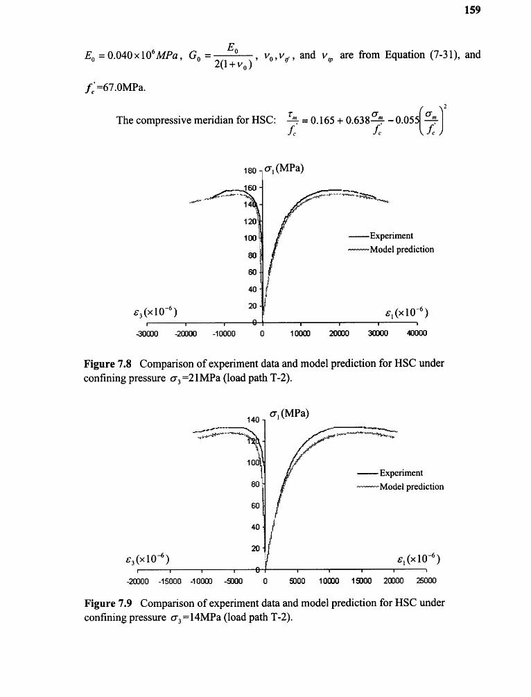
159

CHAPTER 8
CONCLUsIONs
8.1 On Uniaxial Compression of HsC and SFHSC
1) The lateral strain at the end of the cylinder is much less than that right at the mid-
height of the cylinder under the rigid loading platen, indicating a substantial confinement
at both ends imposed by the platen. While the designed flexible loading platen tends to
diminish this confinement, especially for cylinders with an h/d ratio of 1.5 which
essentially has the same lateral strains at ends and mid-height, a clear sign of
comparatively better uniform expansion under fairly "true" uniaxial compression.
2) Under the rigid loading platen, the uniaxial compressive strength of SFHSC increases
as the h/d ratio decreases, but for the designed lubricated loading platen, the same
strength for all hid ratios (1.0, 1.5 and 2.0) is achieved.
3) Under the lubricated loading platen, the concrete undergoes volume contraction all the
way to around 95% of the ultimate strength when it starts to dilate. The variation of the
bulk modulus (K) of steel fiber reinforced HSC within a certain deformation range
(s / e < 2.0) can be simulated by two straight lines, representing ascending and
descending part respectively. The slope of the descending part is about 5%-7% of that of
the initial ascending part.
160

161
4) The secant Poisson's ratio below 70% of the peak stress and the tangential Poisson's
ratio below 50% of the peak stress for SFHSC under different loading platens are
essentially the same, to which a constant of 0.200.22 can be applied. Beyond those
ranges, the Poisson's ratios under lubricated and rigid loading platens experience
increasing divergence from each other.
5) Kupfer's equation, originally used for the ordinary concrete, can be adopted to express
the variation of the tangential Poisson's ratio of SFHSC before failure:
6) Within a certain range after failure (El E.< 2.0), the tangential Poisson's ratio of
SFHSC can be reasonably taken as a constant, 1.35.
7) The secant Poisson's ratio of SFHSC can be expressed using the following three

162
8.2 On Triaxial Compression Tests of HsC and sFHsC
1) Under triaxial compression, Mohr-Coulomb failure criterion can be applied to both
HSC and SFHSC:
where o is the ultimate axial strength and a y is the ultimate confining pressure up to 70
MPa. The parameter k can be adopted as 4.5 for both HSC and SFHSC, which is about
the mean value of the previous researches on normal strength concrete and HSC found in
the literature search. And the introduction of steel fibers does not affect the internal
friction angle 0 in the Mohr-Coulomb failure criterion.
2) Under triaxial compression, the compressive meridians of Willam-Warnke failure
criterion can be written as
Upon comparison between those two, it is found that they are essentially the same
on the ultimate surface.
The compressive meridian for HSC obtained in this study complies well with the
results from Xie (1995) and Pantazopoulou (2001), but deviates from Ansari's findings
(1998). Also it follows the same trend with that from Chern's research (1992) using the
normal strength concrete.

163
With the shortage of such information concerning SFHSC from the previous
studies, the compressive meridian of SFHSC obtained in this study is quite close to
Ishikawa's result (2000). And it also complies well with Chern's result (1992) for steel
fiber reinforced normal strength concrete.
Therefore, it seems that the concrete strength grade and the introduction of the
steel fiber do not have a substantial influence on the compressive meridian on the
ultimate surface of Willam-Warnke failure criterion.
3) For both HSC and SFHSC in tnaxial compression, different load paths considered in
this study (T-1, T-2, T-2', T-3 and T-4) seem to have insignificant effect on the ultimate
strength a l , and the shape of axial stress ~ axial and lateral strain curves and r acm ~ yocmm
curve.
4) For both HSC and SFHSC, the relationship between the octahedral shear stress T acm
and the engineering octahedral shear strain y„,,, under moderate confining pressure (less
than 28MPa) in triaxial compression can be described by Saenz equation:

164
5) Good relationships between the peak octahedral shear stress rocip and the peak
engineering octahedral shear strain y,,,mp exist for both HSC and SFHSC under triaxial
compression. They can be expressed as Tom = 1.458 x10 -y y„,mp + 29.30 for HSC and
Those two equations are almost the same when
plotted on the same graph, and therefore can be represented by a single equation.
As discussed in Chapter 7, this romp ~ yoemp relationship is of great importance in
establishing the simple constitutive model for both HSC and SFHSC under triaxial
compression in that the peak octahedral shear strain y,,,, p can be predicted through Tacos ,
which can be easily obtained from the ultimate stress surface. And then yocip and rocip are
used to describe the variation of Elastic modulus and Poisson's ratio with stress status.
6) The initial tangent Poisson's ratio o (0.10-0.20) for both HSC and SFHSC under
triaxial compression is lower than their uniaxial counterparts (around 0.20). The variation
of R, with stress status for HSC and SFHSC under triaxial compression can be expressed
as follows:

165
octahedral shear strews( r.ct) ~ engineering octahedral shear strain ( f oe, ) curves of HSC
and SFHSC under triaxial compression. However, slope degradation on the cyclic
branches does occur and becomes worse with the increase of the cycle numbers. But
there seems to be no apparent changing rule for this degradation.
8) The axial strain ( e l ) — lateral strain (63 ) relationship at the cyclic branches does not
deviate much from the mainstream 6, ~ 63 curve for both HSC and SFHSC under
triaxial compression. This phenomenon indicates a fair assumption can be made that the
tangent Poisson's ratio along the cyclic branches is equal to that value at the unloading
point of the stress ~ strain curve.
9) From this study, it is found that the introduction of steel fiber into the HSC does not
seem to provide any remarkable advantages in terms of strength and ductility over the
normal HSC under triaxial compression.
8.3 On Incremental Constitutive Model for HsC and sFHsC
1) In order to establish the incremental constitutive model to simulate the whole load
deformation process of concrete, the stress — strain relationship needs to be correctly
defined. The most commonly used method is to simulate the concrete behavior under
multiaxial stress conditions by copying the uniaxial stress ~ strain relationship. Thus the
concept of equivalent uniaxial strain was developed to determine the variation of tangent
elastic moduli Et and Poisson's ratios t in all directions.

166
However, this equivalent uniaxial strain is fictitious and based on unverified
assumptions, and its ultimate surface is hard to get and highly dependent on each specific
case. Therefore, when applied to the model analysis, it will lead to a big discrepancy that
the peak stress and peak equivalent uniaxial strain do not occur simultaneous, which
makes the analysis results highly unreliable.
2) The experimental program of this study has shown good relationships between the
peak octahedral shear stress rac!, and the peak engineering octahedral shear strain
for both HSC and SFHSC under uniaxial compression. So under proportional loading, the
peak strain value Cad can be clearly determined through the peak stress a, by the
ultimate surface of stress. Therefore, the 'racm yoc curve (ascending and descending
branches) can be defined by using the Saenz equation. And then the relationship between
the elastic modulus E„ shear modulus Gm and Poisson's ratio R, is employed to achieve
the variation of Em which is to be adopted in the constitutive equation.
This proposed model based on the octahedral shear stress ~ strain relationship is
physically clear and every parameter needed is clearly defined rather than assumed. The
advantage is that it can achieve a occurrence simultaneity of peak stress and peak strain,
which is of great importance in simulating the whole deformation process of both SFHSC
and HSC, including the descending branch.
3) The model prediction complies well with the experimental results of HSC and SFHSC
in triaxial compression under moderate confining pressures.

APPENDIX A
TRIAXIAL sTREss ~ sTRAIN CURVEs OF sFHsC IN CYCLIC LOADINGUNDER DIFFERENT CONFINING PREssUREs AND LOAD PATHs
This appendix contains the triaxial stress ~ strain relationship curves for the SFHSC in
cyclic loading under different confining pressures (a y = 7 ~ 70 MPa) and load paths (T-2,
T-2', T-3 and T-4). They are arranged in groups by the specific load condition, and the
graphs from the first to the third of each group are the axial stress (a A ) versus the axial
strain (A s ) and lateral strain (ey ) curves, the octahedral normal stress (60,3 versus the
volume change (360,m) curve and the octahedral shear stress (r ocm) versus the engineering
octahedral shear strain (y„,m) curve, respectively.
167

168

-15000 -10000 -5000 0 5000
360m (x 10 -6 )
ace MPa)50
50
50
30
20
10
-30030 -20030 -15000 0 1 0000 20000 30000 50000 50000
acem (MPa)
I
10000 20000 30000 50000 50300 50000 70000
Figure A.2 uniaxial stress ~ strain curves in cyclic loading under confining pressure63=14MPa (load path T-2).
70 -
50 -
50 -
50 -
30 -
20 -
10 -
0 0
169
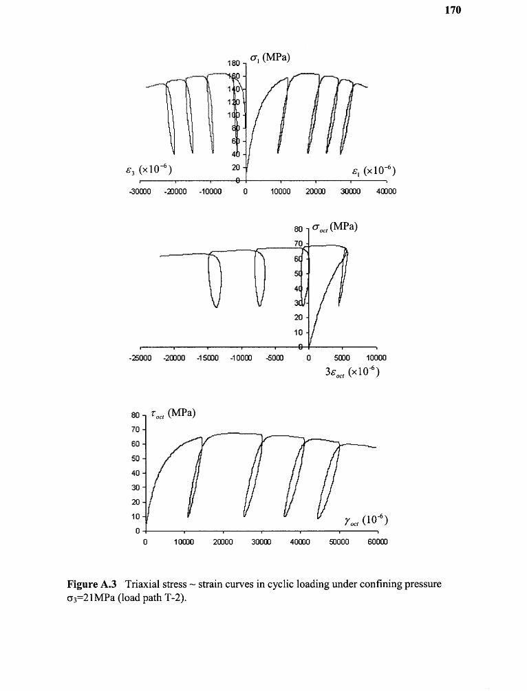
Figure A.3 uniaxial stress ~ strain curves in cyclic loading under confining pressure6 y=21MPa (load path T-2).
170

Figure A.4 Triaxial stress ~ strain curves in cyclic loading under confining pressure63=28MPa (load path T-2).
171

172

173
Figure A.6 uniaxial stress ~ strain curves in cyclic loading under confining pressure3=28MPa (load path T-3).

174

175
Figure A.8 uniaxial stress ~ strain curves in cyclic loading under confining pressure63=42MPa (load path T-2').

Figure A.9 uniaxial stress ~ strain curves in cyclic loading under confining pressure63=56MPa (load path T-2').
176
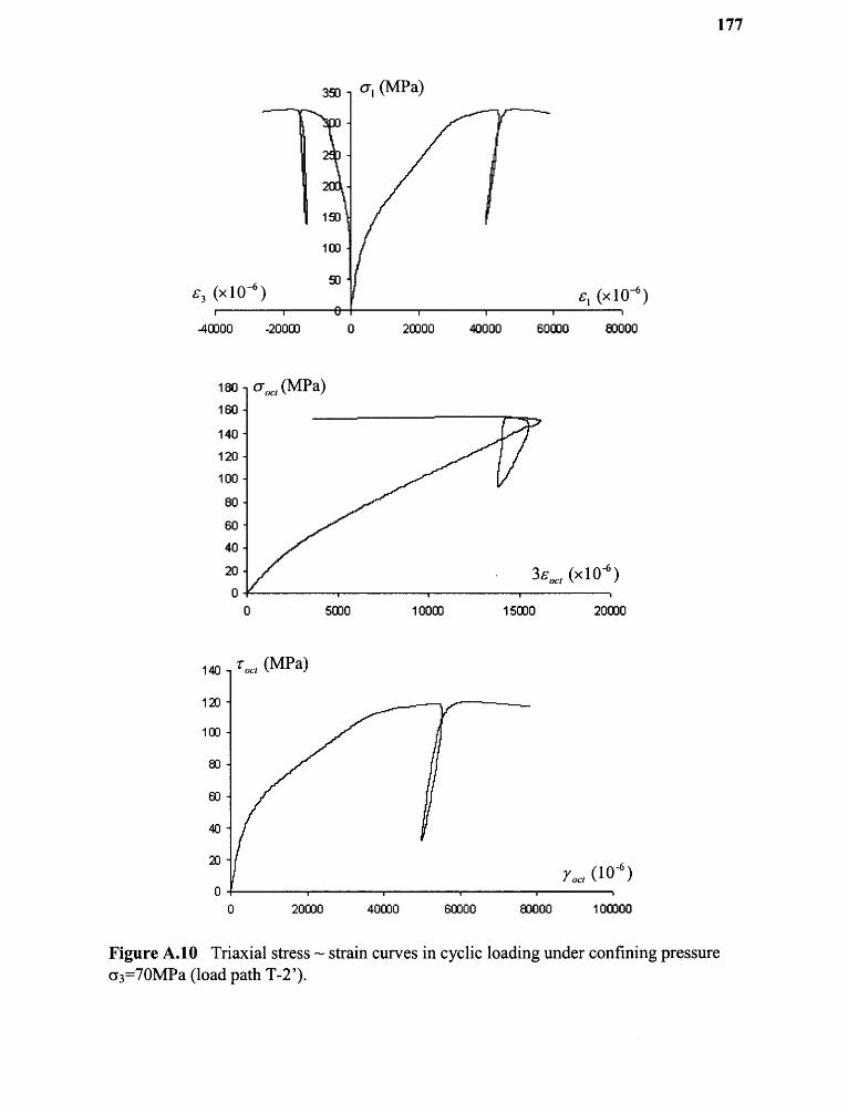
177
Figure A.10 Triaxial stress ~ strain curves in cyclic loading under confining pressure63=14MPa (load path T-2').

APPENDIX B
LATERAL sTRAIN ~ AXIAL sTRAIN RELATIONsHIP DURINGCYCLIC LOADING FOR sFHsC
This appendix presents the axial strain A ~ lateral strain 6.y relationship of SFHSC
during cyclic loading under different confining pressures cr 3 (7MPa to 56MPa) and load
paths (T-2, T-2' and T-4).
178

Figure B.4 Lateral strain s3 ~ axial strain cif during cyclic loading under confiningpressure 6 3=28MPa (load path T-2).
179

Figure B.6 Lateral strain E3 ~ axial strain c1 during cyclic loading under confiningpressure cy3=28MPa (load path T-4).
180

Figure B.8 Lateral strain s3 ~ axial strain s ib during cyclic loading under confiningpressure 63=28MPa (load path T-2').
181

REFERENCEs
Ansari, Farhad and Li, Qingbin (1998), High Strength Concrete Subjected to uniaxialCompression, ACID Materials Journal, November/December 1998.
Bathe, Klaus-Jurgen and Ramaswamy, Seshadri (1979). On Three-DimensionalNonlinear Analysis of Concrete Structures, Nuclear Engineering and Design, 52(1979) 385-409.
Candappa, D. C., Sanjayan, J. G., and Setunge, S. (2001). Complete Stress–Strain Curvesof High Strength Concrete, Journal of Materials in Civil Engineering, May/June2001.
Chen, W. F. (1982). Plasticity in Reinforced Concrete, McAraw-Hill Book Company,
Chern, Jenn-Chuan (1992). Behavior of Steel Fiber Reinforced Concrete in MultiaxialLoading, ACID Materials Journal, Jan.-Feb. 1992.
Darwin, David and Pecknold, David A. (1977). Nonlinear Biaxial Stress-Strain Law forConcrete, Journal of the Engineering Mechanics Division, April 1977, pp229-241.
Elwi, Alai A. and Murray, David W. (1979). A 3D Hypoelastic Concrete ConstitutiveRelationship, Journal of the Engineering Mechanics Division, August 1979.
Gao, Jianming, Sun, Wei, and Morino, Keiji (1997). Mechanical Properties of SteelFiber-reinforced, High-strength, Lightweight Concrete, Cement and Concrete Composite 19 (1997).
Gerstie, Kurt H. (1981). Simple Formulation of Biaxial Concrete Behavior, Journal ofAmerican Concrete Institute, Jan.-Feb. 1981.
Gerstie, Kurt H., Aschl, Helmut et. al. (1980). Behavior of Concrete under MultiaxialStress States, Journal of the Engineering Mechanics Division, Dec. 1980.
Guo, Zhenhai (1997). Strength and Deformation of Concrete — Experimental Principlesand Constitutive Law (Chinese Edition), Tsinghua University Press House,Beijing, P.R. China.
Imaran, I. and Pantazopoulou, S. J. (1996). Experimental Study of Plain Concrete underTriaxial Stress, ACID Materials Journal, November-December 1996.
182
183
Ishikawa, Tetsuya, Ohnuma, Hiroshi and Izumo, Kenji (2000). A mathematicalDescription of Deformational Behavior of High Strength Concrete Reinforcedwith Steel Fiber under uniaxial Compression, unansactions of the JapanConcrete Institute, Vol.22, 2000.
Kupfer, Helmut B. and Gerstie, Kurt H. (1973). Behavior of Concrete under BiaxialStresses, Journal of the Engineering Mechanics Division, August 1973.
Kupfer, H., Hilsdorf, H. K., and Rusch, H. (1969). Behavior of Concrete under BiaxialStresses, Journal of American Concrete Institute, Vol. 66, No. 8, pp.656-666(1969).
Lan, Shenrui and Guo, Zhenhai (1997). Bxperimental Investigation of MultiaxialCompressive Strength of Concrete under Different Stress Paths, ACI Materials Journal, September-October 1997.
Mindess, Sidney, Young, J. Francis and Darwin, David (2002). Concrete (SecondBdition), Prentice Hall.
Moaveni, Saeed (1999). Finite Blement Analysis — Theory and Application withANSYS, Prentice Hall.
Nielson, Claus Vestergaard (1998). uniaxial Behavior of High Strength Concrete andMotar, ACI Materials Journal, March-April 1998.
Ottosen, Niels Saabye (1979). Constitutive Model For Short-Time Loading Of Concrete,Journal of The Engineering Mechanics Division, February 1979.
Pantazopoulou, S. J. (2001). uniaxial Tests of Fiber-Reinforced Concrete, Journal ofMaterials in Civil Bngineering, September-October 2001.
Persson, Bertil (1999). Poisson's Ratio of High Performance Concrete, Cement andConcrete Research, Vol. 29, 1999, P 1647-1653.
Rashid, M.A., Mansur, M.A., and Paramasivam, P. (2002). Correlations betweenMechanical Properties of High-Strength Concrete, Journal of Materials in Civil Engineering, May/June 2002.
Rock and Concrete Mechanics Testing System (1994), Technical Description, MTSSystem Corp., 1994, Minneapolis, Minn..
Sfer, Domingo and Carol, Ignacio (2002). Study of the Behavior of Concrete underTriaxial Compression, Journal of Engineering Mechanics, February 2002.
Van Mier, J. G. M. et. al (1997). Strain Softening of Concrete in Uniaxial Compression,Materials and Structures, Vol.30, May 1997.

184
Van Vliet, M.R.A. and van Mier, J.G.M (1996). Experimental investigation of concretefracture under uniaxial compression, Mechanics of Cohesive-FrictionalMaterials, Jan. 1996.
Xie, J., Elwi, A.E. and MacAregor, J. G. (1995). Mechanical Properties of Three High-Strength Concretes Containing Silica Fume, ACID Materials Journal, March-April 1995.
Zhu, Bofang (1998). The Finite Element Method Theory and Applications (ChineseEdition), The Water Resources Publishing House of China, Beijing, P.R. China.