copyright © cengage learning. all rights reserved. 13 nonlinear and multiple regression

Copyright © Cengage Learning. All rights reserved.

13 Nonlinear and Multiple Regression

Copyright © Cengage Learning. All rights reserved.

13.1 Assessing Model Adequacy

3

Assessing Model Adequacy

A plot of the observed pairs (xi, yi) is a necessary first step in deciding on the form of a mathematical relationship between x and y.

It is possible to fit many functions other than a linear one (y = b0 + b1x) to the data, using either the principle of least squares or another fitting method.

Once a function of the chosen form has been fitted, it is important to check the fit of the model to see whether it is in fact appropriate.

4

Assessing Model Adequacy

One way to study the fit is to superimpose a graph of the best-fit function on the scatter plot of the data.

However, any tilt or curvature of the best-fit function may obscure some aspects of the fit that should be investigated.

Furthermore, the scale on the vertical axis may make it difficult to assess the extent to which observed values deviate from the best-fit function.

5

Residuals and Standardized Residuals

6


A more effective approach to assessment of model adequacy is to compute the fitted or predicted values and the residuals ei = yi – and then plot various functions of these computed quantities.

We then examine the plots either to confirm our choice of model or for indications that the model is not appropriate. Suppose the simple linear regression model is correct, and let be the equation of the estimated regression line. Then the ith residual is ei = yi – .

7


To derive properties of the residuals, let represent the ith residual as a random variable (rv) before observations are actually made. Then

Because is a linear function of the Yj’s, so is Yi – (the coefficients depend on the xj’s). Thus the normality of the Yj’s implies that each residual is normally distributed.

(13.1)

8


It can also be shown that

Replacing 2 by s2 and taking the square root of Equation (13.2) gives the estimated standard deviation of a residual.

Let’s now standardize each residual by subtracting the mean value (zero) and then dividing by the estimated standard deviation.

(13.2)

9


The standardized residuals are given by

If, for example, a particular standardized residual is 1.5, then the residual itself is 1.5 (estimated) standard deviations larger than what would be expected from fitting the correct model.

(13.3)

10


Notice that the variances of the residuals differ from one another. In fact, because there is a – sign in front of (xi – x)2, the variance of a residual decreases as xi moves further away from the center of the data x.

Intuitively, this is because the least squares line is pulled toward an observation whose xi value lies far to the right or left of other observations in the sample.

Computation of the can be tedious, but the most widely used statistical computer packages will provide these values and construct various plots involving them.

11

Example 1

We already know the presented data on x = burner area liberation rate and y = NOx emissions.

Here we reproduce the data and give the fitted values, residuals, and standardized residuals. The estimated regression line is y = –45.55 + 1.71x, and r2 = .961.

The standardized residuals are not a constant multiple of the residuals because the residual variances differ somewhat from one another.

12

Example 1

.

cont’d

13

Diagnostic Plots

14

Diagnostic Plots

The basic plots that many statisticians recommend for anassessment of model validity and usefulness are the following:

1. ei (or ei) on the vertical axis versus xi on the horizontal

axis

2. ei (or ei) on the vertical axis versus on the horizontal

axis

3. on the vertical axis versus yi on the horizontal axis

4. A normal probability plot of the standardized residuals

15

Diagnostic Plots

Plots 1 and 2 are called residual plots (against the independent variable and fitted values, respectively), whereas Plot 3 is fitted against observed values.

If Plot 3 yields points close to the 45° line [slope +1 through (0, 0)], then the estimated regression function gives accurate predictions of the values actually observed.

Thus Plot 3 provides a visual assessment of model effectiveness in making predictions. Provided that the model is correct, neither residual plot should exhibit distinct patterns.

16

Diagnostic Plots

The residuals should be randomly distributed about 0 according to a normal distribution, so all but a very few standardized residuals should lie between –2 and +2 (i.e., all but a few residuals within 2 standard deviations of their expected value 0).

The plot of standardized residuals versus is really a combination of the two other plots, showing implicitly both how residuals vary with x and how fitted values compare with observed values.

17

Diagnostic Plots

This latter plot is the single one most often recommended for multiple regression analysis.

Plot 4 allows the analyst to assess the plausibility of the assumption that has a normal distribution.

18

Example 2

Example 1. . . continued

Figure 13.1 presents a scatter plot of the data and the four plots just recommended.

Figure 13.1

Plots for the data from Example 1

19

Example 2

.

cont’d

Figure 13.1


20

Example 2

.

Figure 13.1


cont’d

21

Example 2

The plot of versus y confirms the impression given by r2 that x is effective in predicting y and also indicates that there is no observed y for which the predicted value is terribly far off the mark.

Both residual plots show no unusual pattern or discrepant values. There is one standardized residual slightly outside the interval (–2, 2), but this is not surprising in a sample of size 14.

The normal probability plot of the standardized residuals is reasonably straight. In summary, the plots leave us with no qualms about either the appropriateness of a simple linear relationship or the fit to the given data.

cont’d

22

Difficulties and Remedies

23


Although we hope that our analysis will yield plots like those of Figure 13.1, quite frequently the plots will suggest one or more of the following difficulties:

1. A nonlinear probabilistic relationship between x and y is appropriate.

2. The variance of (and of Y) is not a constant 2 but depends on x.

3. The selected model fits the data well except for a very few discrepant or outlying data values, which may have greatly influenced the choice of the best-fit function.

24


4. The error term does not have a normal distribution.

5. When the subscript i indicates the time order of the observations, the i’s exhibit dependence over time.

6. One or more relevant independent variables have been omitted from the model.

25


Figure 13.2 presents residual plots corresponding to items 1–3, 5, and 6. We discussed patterns in normal probability plots that cast doubt on the assumption of an underlying normal distribution.

(a) (b)

Figure 13.2

(a) nonlinear relationship; (b) nonconstant variance;

Plots that indicate abnormality in data:

26


.

(c) (d)

Figure 13.2

(c) discrepant observation; (d) observation with large influence;


cont’d

27


.

(e) (f)

Figure 13.2


(e) dependence in errors; (f) variable omitted

cont’d

28


Notice that the residuals from the data in Figure 13.2(d) with the circled point included would not by themselves necessarily suggest further analysis, yet when a new line is fit with that point deleted, the new line differs considerably from the original line.

This type of behavior is more difficult to identify in multiple regression. It is most likely to arise when there is a single (or very few) data point(s) with independent variable value(s) far removed from the remainder of the data.

We now indicate briefly what remedies are available for the types of difficulties.

29


For a more comprehensive discussion, one or more of the references on regression analysis should be consulted. If the residual plot looks something like that of Figure 13.2(a), exhibiting a curved pattern, then a nonlinear function of x may be fit.

Figure 13.2(a)

30


The residual plot of Figure 13.2(b) suggests that, although a straight-line relationship may be reasonable, the assumption that V(Yi) = 2 for each i is of doubtful validity.

Figure 13.2(b)

31


When the assumptions as studied earlier are valid, it can be shown that among all unbiased estimators of 0 and 1, the ordinary least squares estimators have minimum variance.

These estimators give equal weight to each (xi, Yi). If the variance of Y increases with x, then Yi’s for large xi should be given less weight than those with small xi. This suggests that 0 and 1 should be estimated by minimizing

fw(b0, b1) = wi[yi – (b0 + b1xi)]2

where the wi’s are weights that decrease with increasing xi.

32


Minimization of Expression (13.4) yields weighted least squares estimates. For example, if the standard deviation of Y is proportional to x (for x > 0)—that is, V(Y) = kx2—then it can be shown that the weights wi = yield best estimators of 0 and 1.

The books by John Neter et al. and by S. Chatterjee and Bertram Price contain more detail.

Weighted least squares is used quite frequently by econometricians (economists who use statistical methods) to estimate parameters.

33


When plots or other evidence suggest that the data set contains outliers or points having large influence on the resulting fit, one possible approach is to omit these outlying points and recompute the estimated regression equation.

This would certainly be correct if it were found that the outliers resulted from errors in recording data values or experimental errors.

If no assignable cause can be found for the outliers, it is still desirable to report the estimated equation both with and without outliers omitted.

34


Yet another approach is to retain possible outliers but to use an estimation principle that puts relatively less weight on outlying values than does the principle of least squares.

One such principle is MAD (minimize absolute deviations), which selects and to minimize | yi – (b0 + b1xi |.

Unlike the estimates of least squares, there are no nice formulas for the MAD estimates; their values must be found by using an iterative computational procedure.

35


Such procedures are also used when it is suspected that the i’s have a distribution that is not normal but instead have “heavy tails” (making it much more likely than for the normal distribution that discrepant values will enter the sample); robust regression procedures are those that produce reliable estimates for a wide variety of underlying error distributions.

Least squares estimators are not robust in the same way that the sample mean X is not a robust estimator for .

36


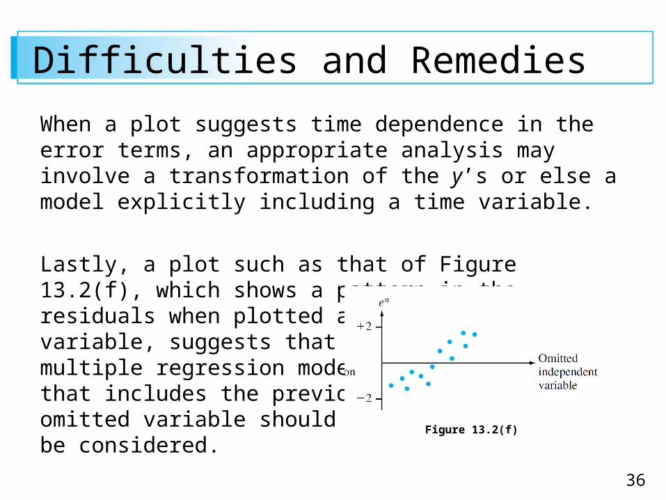
When a plot suggests time dependence in the error terms, an appropriate analysis may involve a transformation of the y’s or else a model explicitly including a time variable.

Lastly, a plot such as that of Figure 13.2(f), which shows a pattern in the residuals when plotted against an omittedvariable, suggests that a multiple regression model that includes the previouslyomitted variable should be considered.

Figure 13.2(f)

copyright © cengage learning. all rights reserved. 13 nonlinear and multiple regression

Documents

standardized residuals

residuals e i

model adequacy slide

ith residual

bestfit function

correct model

multiple regression

residual decreases