copyright by swagata das 2015

Copyright

by

Swagata Das

2015

The Dissertation Committee for Swagata Dascertifies that this is the approved version of the following dissertation:

Fault Location and Analysis in Transmission and Distribution

Networks

Committee:

Surya Santoso, Supervisor

Ross Baldick

Michael F. Becker

Matt Hersh

Thomas A. Short


Networks

by

Swagata Das, B.Tech, M.S.E

DISSERTATION

Presented to the Faculty of the Graduate School of

The University of Texas at Austin

in Partial Fulfillment

of the Requirements

for the Degree of

DOCTOR OF PHILOSOPHY

THE UNIVERSITY OF TEXAS AT AUSTIN

May 2015

Dedicated to my parents and to the loving memory of my grandparents.

Acknowledgments

I wish to thank my advisor, Dr. Surya Santoso, for his invaluable guidance and

support throughout my years at UT-Austin. Working under him has been an absolute

honor and privilege. Everything that I know about power systems, technical writing, and

technical presentation, I have learned from him. Thank you for believing in me and giv-

ing me this incredible opportunity; I am very grateful and very proud to be your student.

I would like to thank Dr. Ross Baldick, Dr. Matt Hersh, Dr. Michael Becker,

and Mr. Thomas A. Short for taking time off their busy schedules and serving on my

dissertation committee. Their comments and suggestions have been invaluable towards

completing this dissertation.

My sincere thanks to Electric Power Research Institute for providing financial

support and actual fault event data used in this research.

I am also very grateful to all the staff members at the Electrical and Computer

Engineering Department and the International Office. Special thanks to Melanie Gulick

and Melody Singleton for being so encouraging and helpful all the time.

Many thanks go out to my fellow labmates with whom I have had a lot of fun

over the last five years. Thank you, Neeraj Karnik, Thekla Boutsika, Pisitpol Chi-

rapongsananurak, Anamika Dubey, Min Lwin, David Jonsson, Tuan Ngo, Kyung Woo

Min, Jules Campbell, Yichuan Niu, Suma Basu, and Jonas Traphoner.

Finally, I would like to express my sincere gratitude to my parents for their love,

encouragement, support, and immense patience.

v


Networks

Swagata Das, Ph.D.

The University of Texas at Austin, 2015

Supervisor: Surya Santoso

Short-circuit faults are inevitable on transmission and distribution networks. In

an effort to provide system operators with an accurate location estimate and reduce

service restoration times, several impedance-based fault location algorithms have been

developed for transmission and distribution networks. Each algorithm has specific in-

put data requirements and make certain assumptions that may or may not hold true in

a particular scenario. Identifying the best fault location approach, therefore, requires

a thorough understanding of the working principle behind each algorithm. Moreover,

impedance-based fault location algorithms require voltage and current phasors, captured

by intelligent electronic devices (IEDs), to estimate the fault location. Unfortunately,

voltage phasors are not always available due to operational constraints or equipment

failure. Furthermore, impedance-based fault location algorithms assume a radial distri-

bution feeder. With increased interconnection of distributed generators (DGs) to the

feeder, this assumption is violated. DGs also contribute to the fault and severely compro-

mise the accuracy of location estimates. In addition, the variability of certain DGs such

as the fixed-speed wind turbine can alter fault current levels and result in relay misop-

erations. Finally, data recorded by IEDs during a fault contain a wealth of information

and are prime for use in other applications that improve power system reliability.

vi

Based on the above background, the first objective of this dissertation is to present

a comprehensive theory of impedance-based fault location algorithms. The contributions

lie in clearly specifying the input data requirement of each algorithm and identifying their

strengths and weaknesses. The following criteria are recommended for selecting the most

suitable fault location algorithm: (a) data availability and (b) application scenario. The

second objective is to develop fault location algorithms that use only the current to

estimate the fault location. The simple but powerful algorithms allow system operators

to locate faults even in the absence of voltage data. The third objective is to investigate

the shortcomings of existing fault location algorithms when DGs are interconnected to

the distribution feeder and develop an improved solution. A novel algorithm is proposed

that require only the voltage and current phasors at the substation, is straightforward to

implement, and is capable of locating all fault types. The fourth objective is to examine

the effects of wind speed variation on the maximum and minimum fault current levels of

a wind turbine and investigate the impact on relay settings. Contributions include devel-

oping an accurate time-domain model of a fixed-speed wind turbine with tower shadow

and wind shear and verifying that the variation in wind speed does not violate relay

settings calculated using the IEC 60909-0 Standard. The final objective is to exploit

intelligent electronic device data for improving power system reliability. Contributions

include validating the zero-sequence impedance of multi-terminal transmission lines with

unsynchronized measurements, reconstructing the sequence of events, assessing relay per-

formance, estimating the fault resistance, and verifying the accuracy of the system model.

Overall, the research presented in this dissertation aims to describe the theory

of impedance-based fault location, identify the sources of fault location error, propose

solutions to overcome those error sources, and share lessons learned from analyzing

intelligent electronic device data. The research is expected to reduce service downtime,

prevent protection system misoperations, and improve power quality.

vii

Table of Contents

Acknowledgments v

Abstract vi

List of Tables xiii

List of Figures xvi

Chapter 1. Introduction 1

1.1 Background and Motivation . . . . . . . . . . . . . . . . . . . . . . . . . 1

1.2 Objectives . . . . . . . . . . . . . . . . . . . . . . . . . . . . . . . . . . . 7

1.3 Original Research Contributions and Dissertation Outline . . . . . . . . . 9

Chapter 2. Theory of Impedance-based Fault Location Algorithms 15

2.1 One-ended Impedance-based Fault Location Algorithms . . . . . . . . . . 16

2.1.1 Simple Reactance Method . . . . . . . . . . . . . . . . . . . . . . . 19

2.1.2 Takagi Method . . . . . . . . . . . . . . . . . . . . . . . . . . . . . 20

2.1.3 Modified Takagi Method . . . . . . . . . . . . . . . . . . . . . . . . 22

2.1.4 Eriksson Method . . . . . . . . . . . . . . . . . . . . . . . . . . . . 23

2.1.5 Novosel et al. Method . . . . . . . . . . . . . . . . . . . . . . . . . 24

2.2 Two-ended Impedance-based Fault Location Algorithms . . . . . . . . . . 26

2.2.1 Synchronized Two-ended Method . . . . . . . . . . . . . . . . . . . 26

2.2.2 Unsynchronized Two-ended Method . . . . . . . . . . . . . . . . . 28

2.2.3 Unsynchronized Current-only Two-ended Method . . . . . . . . . . 29

2.3 Summary . . . . . . . . . . . . . . . . . . . . . . . . . . . . . . . . . . . . 30

Chapter 3. Error Analysis of Impedance-based Fault Location 32

3.1 Benchmark Test Case . . . . . . . . . . . . . . . . . . . . . . . . . . . . . 33

3.2 Fault Location Error due to Inaccurate Input Data . . . . . . . . . . . . 35

3.2.1 Inaccurate Current Phasor: DC Offset and CT Saturation . . . . . 35

3.2.2 Inaccurate Voltage Phasor: Delta-connected Potential Transformer 38

3.2.3 Inaccurate Line Parameters: Untransposed Lines . . . . . . . . . . 39

3.2.4 Inaccurate Line Parameters: Uncertainty in Earth Resistivity . . . 41

viii

3.2.5 Inaccurate Line Parameters: Tower Footing Resistance . . . . . . . 44

3.2.6 Inaccurate Line Parameters: Earth Current Return Model . . . . . 48

3.2.7 Inaccurate Line Parameters: Non-homogeneous Lines . . . . . . . . 51

3.3 Fault Location Error due to Application Challenges . . . . . . . . . . . . 52

3.3.1 System Load . . . . . . . . . . . . . . . . . . . . . . . . . . . . . . 52

3.3.2 Non-homogeneous System . . . . . . . . . . . . . . . . . . . . . . . 54

3.3.3 Parallel Lines . . . . . . . . . . . . . . . . . . . . . . . . . . . . . . 55

3.3.4 Three-terminal Lines . . . . . . . . . . . . . . . . . . . . . . . . . . 59

3.3.5 Tapped Radial Line . . . . . . . . . . . . . . . . . . . . . . . . . . 60

3.4 Application of Impedance-based Fault Location Algorithms to Field Data 62

3.4.1 Event 1: Lightning Strike on a 161-kV Transmission Line - Suc-cessful Fault Location from One-ended Methods . . . . . . . . . . 62

3.4.2 Event 2: Bird Contact with a 161-kV Transmission Line - SuperiorPerformance of Two-ended Methods over One-ended Methods . . . 64

3.4.3 Event 3: Lightning Strike on a 161-kV Transmission Line - IncorrectApplication or Inaccurate Input Causes Two-ended Methods to Fail 67

3.4.4 Event 4: A-G Fault Location on a 34.5-kV Distribution Feeder withLine-to-Line Voltages . . . . . . . . . . . . . . . . . . . . . . . . . 71

3.4.5 Event 5: Tree Contact Fault with a 34.5-kV Distribution Feeder -Challenging Fault with a Variable Fault Resistance . . . . . . . . . 75

3.4.6 Event 6: Transformer Inrush Mistaken as a Fault on a 4.16-kVDistribution Feeder - Filtered vs. Unfiltered Events . . . . . . . . . 77

3.5 Summary . . . . . . . . . . . . . . . . . . . . . . . . . . . . . . . . . . . . 80

Chapter 4. Fault Location Algorithms using Current Only 81

4.1 Fault Location using Current Phasors . . . . . . . . . . . . . . . . . . . . 83

4.2 Fault Location using Current Magnitude . . . . . . . . . . . . . . . . . . 87

4.3 Demonstration using a Benchmark Test Case . . . . . . . . . . . . . . . . 92

4.4 Application to Field Data . . . . . . . . . . . . . . . . . . . . . . . . . . . 94

4.4.1 Event 1: Recloser Failure on a 34.5-kV Distribution Feeder . . . . 95

4.4.2 Event 2: Tree Contact Fault with a 8.32-kV Distribution Feeder . . 98

4.4.3 Fault Location Analysis of the Remaining Events . . . . . . . . . . 101

4.5 Short-circuit Fault Current Profile Method . . . . . . . . . . . . . . . . . 103

4.6 Summary . . . . . . . . . . . . . . . . . . . . . . . . . . . . . . . . . . . . 103

ix

Chapter 5. Effects of Distributed Generators on Fault Location 104

5.1 Impact of DGs on Impedance-based Fault Location . . . . . . . . . . . . 106

5.2 Distribution Test Case Feeder . . . . . . . . . . . . . . . . . . . . . . . . 108

5.3 Factors that Affect Fault Location Downstream from DGs . . . . . . . . . 111

5.3.1 DG Technology . . . . . . . . . . . . . . . . . . . . . . . . . . . . . 111

5.3.2 DG Interconnect Transformer . . . . . . . . . . . . . . . . . . . . . 112

5.3.3 Size of the DG Unit . . . . . . . . . . . . . . . . . . . . . . . . . . 112

5.3.4 Fault Distance from the DG Unit . . . . . . . . . . . . . . . . . . . 113

5.3.5 Fault Resistance . . . . . . . . . . . . . . . . . . . . . . . . . . . . 114

5.3.6 Tapped Load . . . . . . . . . . . . . . . . . . . . . . . . . . . . . . 115

5.4 Summary . . . . . . . . . . . . . . . . . . . . . . . . . . . . . . . . . . . . 117

Chapter 6. An Impedance-based Fault-Locating Technique for Distribu-tion Networks with Distributed Generators 118

6.1 Overview of the Proposed Approach . . . . . . . . . . . . . . . . . . . . . 119

6.2 Step-by-Step Derivation of the Proposed Approach . . . . . . . . . . . . . 119

6.3 Description of the Test Distribution Feeder . . . . . . . . . . . . . . . . . 125

6.4 Application of the Proposed Method . . . . . . . . . . . . . . . . . . . . . 128

6.4.1 Case 1: Estimating the Distance to a ABC Fault at 13.08 miles . . 128

6.4.2 Case 2: Estimating the Distance to a AB Fault at 12.46 miles . . . 128

6.5 Summary . . . . . . . . . . . . . . . . . . . . . . . . . . . . . . . . . . . . 129

Chapter 7. Effects of Distributed Generators on Relay Settings 130

7.1 Maximum and Minimum Fault Currents from a Fixed-speed Wind Turbine133

7.1.1 IEC 60909-0 Standard . . . . . . . . . . . . . . . . . . . . . . . . . 133

7.1.2 Alternative Approach . . . . . . . . . . . . . . . . . . . . . . . . . 134

7.2 Time-domain Modeling of a Fixed-speed Wind Turbine . . . . . . . . . . 137

7.3 Analysis of Wind Speed Variation on Fault Currents . . . . . . . . . . . . 140

7.3.1 Approach for Analysis . . . . . . . . . . . . . . . . . . . . . . . . . 140

7.3.2 Case Study: Fixed-speed Wind Turbine and a Weak Grid . . . . . 143

7.3.3 Case Study: Fixed-speed Wind Turbine and a Strong Grid . . . . . 148

7.3.4 Case Study: Fixed-speed Wind Farm and a Strong Grid . . . . . . 149

7.3.5 Case Study: Fixed-speed Wind Turbine with 3p and a Weak Grid . 151

7.3.6 Case Study: Fixed-speed Wind Farm with 3p and a Weak Grid . . 153

7.4 Summary . . . . . . . . . . . . . . . . . . . . . . . . . . . . . . . . . . . . 155

x

Chapter 8. Analysis of Intelligent Electronic Device Data 156

8.1 Assess Relay Performance . . . . . . . . . . . . . . . . . . . . . . . . . . 158

8.2 Validate the Zero-sequence Impedance of Two-terminal Lines . . . . . . . 159

8.2.1 Approach 1: Data from One Terminal . . . . . . . . . . . . . . . . 161

8.2.2 Approach 2: Data from Two Terminals . . . . . . . . . . . . . . . 164

8.2.3 Demonstration using a Benchmark Test Case . . . . . . . . . . . . 166

8.3 Validate the Zero-sequence Impedance of Three-terminal Lines . . . . . . 169

8.3.1 Approach 1: Data from Three Terminals . . . . . . . . . . . . . . . 170



8.4 Estimate the Fault Resistance . . . . . . . . . . . . . . . . . . . . . . . . 179

8.4.1 Approach 1: Data from One Terminal . . . . . . . . . . . . . . . . 179



8.5 Estimate the Thevenin Impedance . . . . . . . . . . . . . . . . . . . . . . 182

8.6 Verify the Power System Model . . . . . . . . . . . . . . . . . . . . . . . 184

8.7 Summary . . . . . . . . . . . . . . . . . . . . . . . . . . . . . . . . . . . . 185

Chapter 9. Demonstration of the Benefits of Analyzing Intelligent Elec-tronic Device Data using Field Data 186

9.1 Case Study 1: Distribution Fault Analysis Reveals Incorrect Line Impe-dance Setting . . . . . . . . . . . . . . . . . . . . . . . . . . . . . . . . . 186

9.1.1 System Protection Description . . . . . . . . . . . . . . . . . . . . 188

9.1.2 Event Report Trigger Criteria . . . . . . . . . . . . . . . . . . . . . 191

9.1.3 Event Reconstruction . . . . . . . . . . . . . . . . . . . . . . . . . 192

9.1.4 Fault Location Discrepancy Analysis . . . . . . . . . . . . . . . . . 195

9.1.5 Evolving Fault Analysis . . . . . . . . . . . . . . . . . . . . . . . . 197

9.1.6 Lessons Learned . . . . . . . . . . . . . . . . . . . . . . . . . . . . 198

9.2 Case Study 2: Tree Contact with a 161-kV Transmission Line Reveals theUpstream Network Response to a Fault . . . . . . . . . . . . . . . . . . . 199


9.2.2 Fault Location . . . . . . . . . . . . . . . . . . . . . . . . . . . . . 200

9.2.3 Fault Resistance Estimation . . . . . . . . . . . . . . . . . . . . . . 203

9.2.4 Thevenin Impedance Estimation . . . . . . . . . . . . . . . . . . . 203

9.2.5 Lessons Learned . . . . . . . . . . . . . . . . . . . . . . . . . . . . 204

9.3 Case Study 3: Failed Line Arrestor on a 161-kV Transmission Line Vali-dates the Zero-sequence Line Impedance . . . . . . . . . . . . . . . . . . 204

9.3.1 Fault Location . . . . . . . . . . . . . . . . . . . . . . . . . . . . . 205

xi



9.3.4 Zero-sequence Line Impedance Validation . . . . . . . . . . . . . . 207

9.3.5 Lessons Learned . . . . . . . . . . . . . . . . . . . . . . . . . . . . 208

9.4 Case Study 4: B-G Fault Verifies Relay Performance, Validates the Zero-sequence Line Impedance, and Authenticates the System Model . . . . . 209

9.4.1 System Protection Description . . . . . . . . . . . . . . . . . . . . 210

9.4.2 Event Report Trigger Criteria . . . . . . . . . . . . . . . . . . . . . 212


9.4.4 Relay Performance Assessment . . . . . . . . . . . . . . . . . . . . 216

9.4.5 Fault Location . . . . . . . . . . . . . . . . . . . . . . . . . . . . . 218



9.4.8 Zero-sequence Line Impedance Validation . . . . . . . . . . . . . . 220

9.4.9 Short-circuit Model Verification . . . . . . . . . . . . . . . . . . . . 220

9.4.10 Lessons Learned . . . . . . . . . . . . . . . . . . . . . . . . . . . . 223

9.5 Case Study 5: Lightning Strike on a 161-kV Transmission Line RevealsIncorrect CT Polarity and Missing Phase CT . . . . . . . . . . . . . . . . 223

9.5.1 Fault Location . . . . . . . . . . . . . . . . . . . . . . . . . . . . . 225



9.5.4 Lessons Learned . . . . . . . . . . . . . . . . . . . . . . . . . . . . 227

9.6 Summary . . . . . . . . . . . . . . . . . . . . . . . . . . . . . . . . . . . . 228

Chapter 10. Conclusion 230

Appendix 234

Appendix A. Line Constant Calculation 235

A.1 Self and Mutual Line Impedance . . . . . . . . . . . . . . . . . . . . . . . 235

A.1.1 Full Carson’s Model . . . . . . . . . . . . . . . . . . . . . . . . . . 235

A.1.2 Modified Carson’s Model . . . . . . . . . . . . . . . . . . . . . . . 237

A.1.3 Deri Model . . . . . . . . . . . . . . . . . . . . . . . . . . . . . . . 238

A.2 Phase Impedance Matrix . . . . . . . . . . . . . . . . . . . . . . . . . . . 239

A.3 Positive- and Zero-sequence Line Impedances . . . . . . . . . . . . . . . 240

A.4 Summary . . . . . . . . . . . . . . . . . . . . . . . . . . . . . . . . . . . . 241

Bibliography 242

Vita 252

xii

List of Tables

2.1 Definition of VG, IG, and ∆IG for Different Fault Types . . . . . . . . . . 18

2.2 Summary of Input Data Requirements of Impedance-based Fault LocationAlgorithms . . . . . . . . . . . . . . . . . . . . . . . . . . . . . . . . . . . 31

3.1 Conductor Data . . . . . . . . . . . . . . . . . . . . . . . . . . . . . . . . 35

3.2 Variation of Earth Resistivity with Soil Type [1] . . . . . . . . . . . . . . 42

3.3 Effect of Earth Resistivity on Line Impedance Parameters . . . . . . . . 42

3.4 Impact of RT on the Eriksson Method . . . . . . . . . . . . . . . . . . . 48

3.5 Effect of RT on the Positive- and Zero-sequence Line Impedances . . . . 48

3.6 Impact of RT on the Unsynchronized Two-ended Method . . . . . . . . . 48

3.7 Line Parameters using Different Earth Current Return Models . . . . . . 50

3.8 Fault Location Estimates using Line Parameters Computed by DifferentEarth Return Models . . . . . . . . . . . . . . . . . . . . . . . . . . . . . 51

3.9 Event 1 Fault Location Estimates from One-ended Methods . . . . . . . 64

3.10 Event 2 Location Estimates from One-ended Methods . . . . . . . . . . . 67

3.11 Event 2 Location Estimate from Two-ended Methods . . . . . . . . . . . 67


3.13 Event 3 Location Estimate from Two-ended Methods . . . . . . . . . . . 70


3.15 Summary of Fault-locating Error Sources that Affect Impedance-basedFault Location Algorithms . . . . . . . . . . . . . . . . . . . . . . . . . . 80

4.1 Actual vs. Estimated Fault Location using the Current Phasor Approach 93

4.2 Actual vs. Estimated Fault Location using the Current Magnitude Ap-proach . . . . . . . . . . . . . . . . . . . . . . . . . . . . . . . . . . . . . 94

4.3 Actual vs. Estimated Location using Current Phasors and Current Mag-nitude . . . . . . . . . . . . . . . . . . . . . . . . . . . . . . . . . . . . . 102

5.1 CAT SR4-HV Synchronous Generator Data [2] . . . . . . . . . . . . . . . 111

5.2 Impact of DG MVA Size on Fault Location Algorithms . . . . . . . . . . 113

5.3 Effect of Distance of the Fault from the DG Unit on Fault Location Al-gorithms . . . . . . . . . . . . . . . . . . . . . . . . . . . . . . . . . . . . 114

5.4 Impact of RF on Impedance-based Fault Locating Algorithms when theFault is Downstream from DGs . . . . . . . . . . . . . . . . . . . . . . . 115

5.5 Impact of Load Taps on Fault Locating Algorithms . . . . . . . . . . . . 117

xiii

6.1 Line Impedance Parameters of the 34.5-kV Distribution Feeder . . . . . . 127

6.2 6.6-MW Wind Turbine Data . . . . . . . . . . . . . . . . . . . . . . . . . 127

7.1 Network Data . . . . . . . . . . . . . . . . . . . . . . . . . . . . . . . . . 144

7.2 Fault Current Contribution from the Wind Turbine at Different WindSpeeds . . . . . . . . . . . . . . . . . . . . . . . . . . . . . . . . . . . . . 146

7.3 Fault Current Contribution from the Wind Turbine at Different WindSpeeds . . . . . . . . . . . . . . . . . . . . . . . . . . . . . . . . . . . . . 147

7.4 Fault Current from a 1.5-MW Wind Turbine Connected to a Strong Gridat Different Wind Speeds . . . . . . . . . . . . . . . . . . . . . . . . . . . 149

7.5 Fault Currents from a 4.5-MW Wind Farm Connected to a Strong Gridat Different Wind Speeds . . . . . . . . . . . . . . . . . . . . . . . . . . . 151

7.6 Fault Currents from a 1.5-MW Wind Turbine, Including 3p . . . . . . . . 153

7.7 Fault Currents from a 4.5-MW Wind Farm, Including 3p . . . . . . . . . 154

8.1 Case Study 1: Estimated vs. Actual Zero-sequence Line Impedance . . . 168

8.2 Case Study 2: Estimated vs. Actual Zero-sequence Line Impedance . . . 169

8.3 Case Study: Estimated vs. Actual Zero-sequence Line Impedance . . . . 178

8.4 Case Study: Actual vs. Estimated RF . . . . . . . . . . . . . . . . . . . 182

8.5 Actual vs. Estimated Thevenin Impedances at Terminal G . . . . . . . . 184

9.1 Conductor Data [3] . . . . . . . . . . . . . . . . . . . . . . . . . . . . . . 196

9.2 Location Estimates using Line Impedance Parameters of a Typical 24.9-kV Distribution Feeder having a 336 ACSR Phase and a 500 AAC NeutralConductor is close to the Actual Fault Location . . . . . . . . . . . . . . 197

9.3 Case Study 2 Location Estimates from One-ended Methods . . . . . . . . 202

9.4 Case Study 2 Location Estimate from the Unsynchronized Two-endedMethod . . . . . . . . . . . . . . . . . . . . . . . . . . . . . . . . . . . . 203

9.5 Case Study 2 Estimated Thevenin Impedance . . . . . . . . . . . . . . . 204


9.7 Case Study 3 Location Estimate from the Unsynchronized Two-endedMethod . . . . . . . . . . . . . . . . . . . . . . . . . . . . . . . . . . . . 207

9.8 Case Study 3 Estimated Short-circuit Impedances . . . . . . . . . . . . . 208

9.9 Case Study 3 Setting vs. Estimated Zero-sequence Line Impedance . . . 208

9.10 Conductor Data . . . . . . . . . . . . . . . . . . . . . . . . . . . . . . . . 210


9.12 Estimated Values of Fault Resistance in Case Study 4 . . . . . . . . . . . 219

9.13 Actual vs. Estimated Positive- and Negative-sequence Thevenin Impedances221

9.14 Actual vs. Estimated Zero-sequence Thevenin Impedance . . . . . . . . . 221

9.15 Setting vs. Estimated Zero-sequence Line Impedance . . . . . . . . . . . 221

xiv

9.16 Short-circuit Current in CAPE vs. Actual Measurements from SEL-351R 222

9.17 Location Estimates from One-ended Methods . . . . . . . . . . . . . . . 225

9.18 Case Study 5 Location Estimate from Two-ended Methods . . . . . . . . 226

9.19 Estimated Positive-sequence Source Impedances . . . . . . . . . . . . . . 227

xv

List of Figures

2.1 One-line diagram of a two-terminal network. . . . . . . . . . . . . . . . . 17

2.2 Reactance error in the simple reactance method [4]. . . . . . . . . . . . . 20

2.3 Superposition theorem used to decomposes the network in Fig. 2.1 into aprefault and a “pure” fault during a three-phase fault. . . . . . . . . . . 21

2.4 Zero-sequence network during a ground fault. . . . . . . . . . . . . . . . 23

2.5 Novosel et al. method assumes a constant impedance load model andlumps it at the end of the feeder. . . . . . . . . . . . . . . . . . . . . . . 25

2.6 Negative-sequence network during an unbalanced fault. . . . . . . . . . . 27

3.1 Tower configuration of an actual 69-kV transmission line. . . . . . . . . . 34

3.2 Fault current with a significant DC offset. . . . . . . . . . . . . . . . . . 36

3.3 Cosine filter is more effective in filtering out the DC offset than the FFTfilter. . . . . . . . . . . . . . . . . . . . . . . . . . . . . . . . . . . . . . . 37

3.4 Variation in location estimates from the simple reactance method due toDC Offset. Voltage and current phasors were calculated using the FFTfilter. . . . . . . . . . . . . . . . . . . . . . . . . . . . . . . . . . . . . . . 38

3.5 A transposed transmission line [5]. . . . . . . . . . . . . . . . . . . . . . 40

3.6 Error in fault location due to untransposed transmission lines. . . . . . . 41

3.7 Error in fault location due to uncertainty in earth resistivity. . . . . . . . 43

3.8 Shield wire grounded through tower footing resistances, RT [6]. . . . . . . 45

3.9 Network of the tower footing resistance and the shield wire impedance. . 45

3.10 Transmission line of benchmark test case reduced to 3.73 miles and sup-ported by towers every 1000 feet. . . . . . . . . . . . . . . . . . . . . . . 46

3.11 Transmission line modeled as an n-phase model in PSCAD with the twoshield wires, S1 and S2, grounded through a tower footing resistance RT . 46

3.12 The impedance scan block in PSCAD was used to calculate the zero-sequence line impedance at different tower footing resistance values. . . . 47

3.13 Earth current return in a three-phase four wire multi-grounded system [7]. 49

3.14 Reactance error due to load in the simple reactance method. . . . . . . . 53

3.15 Load has no impact on the Takagi, Modified Takagi, Eriksson, and Two-ended methods. . . . . . . . . . . . . . . . . . . . . . . . . . . . . . . . . 53

3.16 Effect of a non-homogeneous system on impedance-based fault locationalgorithms. . . . . . . . . . . . . . . . . . . . . . . . . . . . . . . . . . . 55

3.17 Double-circuit transmission network. . . . . . . . . . . . . . . . . . . . . 56

3.18 Configuration of an actual 69-kV double-circuit transmission line. . . . . 57

xvi

3.19 Impact of zero-sequence mutual coupling on impedance-based fault loca-tion algorithms. . . . . . . . . . . . . . . . . . . . . . . . . . . . . . . . . 58

3.20 Three-terminal transmission line. . . . . . . . . . . . . . . . . . . . . . . 60

3.21 Fault on a radial feeder tapped from a two-terminal line. . . . . . . . . . 61

3.22 Event 1 is a BC fault at 7.54 miles from Station 1. . . . . . . . . . . . . . 63

3.23 Event 1 waveforms captured by the DFR at Station 1. . . . . . . . . . . 63

3.24 Event 2 is a A-G fault 30.86 miles from Station 1 or 0.44 miles fromStation 2. . . . . . . . . . . . . . . . . . . . . . . . . . . . . . . . . . . . 64

3.25 Event 2 waveforms captured at both line ends. . . . . . . . . . . . . . . . 65

3.26 Event 3 is a AB-G fault 29.49 miles from Station 1. . . . . . . . . . . . . 68

3.27 Event 3 waveforms captured at both line ends. . . . . . . . . . . . . . . . 69

3.28 A third station is suspected to be present between Station 1 and the fault. 71

3.29 Event 4 fault event log from the SEL-251D relay. . . . . . . . . . . . . . 72

3.30 Event 4 utility circuit model in ASPEN OneLiner. . . . . . . . . . . . . . 73

3.31 Event 4 line currents and line-to-line voltages recorded by the SEL-251Drelay. . . . . . . . . . . . . . . . . . . . . . . . . . . . . . . . . . . . . . . 74

3.32 Event 5 fault event log from the SEL-351A relay. . . . . . . . . . . . . . 75

3.33 Event 5 waveforms recorded by the SEL-351A relay. Initially IB= IC=1.8 kA.After 7.5 cycles, IB= IC=2.7 kA. . . . . . . . . . . . . . . . . . . . . . . 76

3.34 Event 6 fault event log from the SEL-351S relay. . . . . . . . . . . . . . . 78

3.35 Window which allows users to download filtered or unfiltered events fromSEL relays. . . . . . . . . . . . . . . . . . . . . . . . . . . . . . . . . . . 78

3.36 Event 6 filtered current waveforms. . . . . . . . . . . . . . . . . . . . . . 79

3.37 Event 6 unfiltered current waveforms. . . . . . . . . . . . . . . . . . . . . 79

4.1 The SEL-551 relay inputs only the current measurements [8]. . . . . . . . 82

4.2 Sequence network during a single line-to-ground fault. . . . . . . . . . . . 85

4.3 Superposition principle used to decompose the distribution network intoa prefault and “pure fault” network during a single line-to-ground fault. . 86

4.4 One-line diagram of the test case. . . . . . . . . . . . . . . . . . . . . . . 92

4.5 Event 1 is a C-G fault on a feeder recloser at 3.07 miles from the substation. 96

4.6 Voltage and current waveforms recorded by the SEL-651R relay. . . . . . 96

4.7 Relay at the substation records only the fault current magnitude. . . . . 97

4.8 Voltage and current waveforms recorded by the SEL-351A relay at thesubstation. Pretend that the voltage waveforms are missing. . . . . . . . 99

4.9 Relay at the substation records only the fault current magnitudes inphases B and C. . . . . . . . . . . . . . . . . . . . . . . . . . . . . . . . . 100

5.1 Distribution feeder with a fault located downstream from the DG. . . . . 106

xvii

5.2 Apparent impedance Zapp from the substation . . . . . . . . . . . . . . . 108

5.3 One-line diagram of the distribution test case feeder. . . . . . . . . . . . 109

5.4 Line geometry of the 13.8-kV overhead distribution feeder. . . . . . . . . 110

5.5 Loads tapped along the entire length of the distribution feeder. . . . . . . 116

6.1 Move the monitoring location “electrically” from the substation to the POI.120


6.3 Superposition principle used to decompose the network into a prefaultand “pure fault” network. . . . . . . . . . . . . . . . . . . . . . . . . . . 123

6.4 One-line diagram of the 34.5-kV distribution feeder. Transformer impedancesare specified on a 100-MVA base. . . . . . . . . . . . . . . . . . . . . . . 126

7.1 Load current from a fixed-speed wind turbine is maximum at rated windspeed. . . . . . . . . . . . . . . . . . . . . . . . . . . . . . . . . . . . . . 136

7.2 Terminal voltage fluctuating at a 3p frequency. . . . . . . . . . . . . . . . 137

7.3 Block diagram of a fixed-speed wind turbine with tower shadow and windshear. . . . . . . . . . . . . . . . . . . . . . . . . . . . . . . . . . . . . . 138

7.4 Illustrating the tower shadow and wind shear effect in wind turbines. . . 140

7.5 Three-phase fault current from a fixed-speed wind turbine. . . . . . . . . 141

7.6 A 1.5-MW fixed-speed wind turbine connected to the distribution grid inPSCAD simulation software. . . . . . . . . . . . . . . . . . . . . . . . . . 143

7.7 The per unit equivalent of the system in Fig. 7.6 on a 20-kV, 6-MVA base.145

7.8 Equivalent circuit of the system in Fig. 7.6 interconnected to a 50-MVAdistribution grid. . . . . . . . . . . . . . . . . . . . . . . . . . . . . . . . 148

7.9 Equivalent circuit of a 4.5-MW wind farm connected to a 500-MVA stronggrid. . . . . . . . . . . . . . . . . . . . . . . . . . . . . . . . . . . . . . . 150

7.10 Fluctuations in the wind turbine terminal voltage are maximum at therated wind speed. . . . . . . . . . . . . . . . . . . . . . . . . . . . . . . . 152

7.11 Fluctuations in the wind farm terminal voltage at the rated wind speed. . 154

8.1 Zero-sequence line impedance setting in SEL relays. Here, Z0MAG andZ0ANG are the magnitude and phase angle of the zero-sequence line impe-dance. . . . . . . . . . . . . . . . . . . . . . . . . . . . . . . . . . . . . . 160


8.3 Sequence network during a double line-to-ground fault. . . . . . . . . . . 164

8.4 Unsynchronized waveform phase-shifted with respect to the synchronizedwaveform. . . . . . . . . . . . . . . . . . . . . . . . . . . . . . . . . . . . 165

8.5 Case study 1 is a AB-G fault, 4 miles from terminal G with RF =0Ω. . . 167

8.6 Case study 2 is a A-G fault, 10 miles from terminal G with RF =5Ω. . . 168

8.7 Three-terminal transmission line. . . . . . . . . . . . . . . . . . . . . . . 170

xviii

8.8 Negative-sequence network of the three-terminal line in Fig. 8.7 during asingle or double line-to-ground fault. . . . . . . . . . . . . . . . . . . . . 172

8.9 Zero-sequence network of the three-terminal line in Fig. 8.7 during a singleor double line-to-ground fault. . . . . . . . . . . . . . . . . . . . . . . . . 174

8.10 Waveforms during a fault can be used to estimate the Thevenin impedance.183

9.1 Utility network diagram showing the fault location. . . . . . . . . . . . . 187

9.2 Fault event log from the digital relay. . . . . . . . . . . . . . . . . . . . . 188

9.3 Event 7 is a BC fault at an estimated location of 5.46 miles. . . . . . . . 189

9.4 Event 6 is a B-G fault at an estimated location of 4.48 miles. . . . . . . . 189

9.5 Event 5 is a BC fault at an estimated location of 5.22 miles. . . . . . . . 190

9.6 Event 4 is a B-G fault at an estimated location of 4.51 miles. . . . . . . . 190

9.7 Event 3 is a BC-G fault at an estimated location of 5.34 miles. . . . . . . 191

9.8 Settings in the digital relay. . . . . . . . . . . . . . . . . . . . . . . . . . 192

9.9 U3 very inverse time-overcurrent curve. TD=1.72 for the phase andTD=2.06 for the ground time-overcurrent element. . . . . . . . . . . . . 195

9.10 Line Configuration of a Typical 24.9-kV Distribution Feeder [3, 9]. . . . . 196

9.11 Stormy weather on 22 July 2010. . . . . . . . . . . . . . . . . . . . . . . 198

9.12 Case study 2 is a AB fault at 2.34 miles from Station 1 or 16.29 milesfrom Station 2. . . . . . . . . . . . . . . . . . . . . . . . . . . . . . . . . 199

9.13 Case study 2 DFR measurements at Station 1, IAF = IBF =4.8 kA. . . . . 201

9.14 Case study 2 DFR measurements at Station 2. . . . . . . . . . . . . . . . 201

9.15 Case study 3 is a A-G fault located 14.90 miles from Station 1 or 6.25miles from Station 2. . . . . . . . . . . . . . . . . . . . . . . . . . . . . . 205

9.16 Case study 3 DFR measurements at Station 1, IAF =3.4 kA. . . . . . . . 205

9.17 Case study 3 DFR measurements at Station 2, IAF =6.1 kA. . . . . . . . 206

9.18 Case study 4 utility circuit model in CAPE software. . . . . . . . . . . . 209

9.19 Overhead transmission line spacing in feet. . . . . . . . . . . . . . . . . . 210

9.20 SEL-351R fault event history. . . . . . . . . . . . . . . . . . . . . . . . . 211

9.21 Settings in the SEL-351R relay. . . . . . . . . . . . . . . . . . . . . . . . 212

9.22 Event 4 voltage and current waveforms at shot= 0. . . . . . . . . . . . . 214




9.26 Functional specifications of the SEL-351R relay [10]. . . . . . . . . . . . . 217

9.27 Fault current in the circuit model matches well with that measured bythe SEL-351R relay in Event 1. . . . . . . . . . . . . . . . . . . . . . . . 222

9.28 Case study 5 is a ABC fault at 5.86 miles from Station 1 or 17.53 milesfrom Station 2. . . . . . . . . . . . . . . . . . . . . . . . . . . . . . . . . 223

xix

9.29 Case study 5 voltage and current waveforms at Station 1. Phase A currentis missing. . . . . . . . . . . . . . . . . . . . . . . . . . . . . . . . . . . . 224

9.30 Case study 5 voltage and current waveforms at Station 2. . . . . . . . . . 224

9.31 Negative distance estimate from Station 2 indicates that the meter direc-tion is reversed. . . . . . . . . . . . . . . . . . . . . . . . . . . . . . . . . 226

10.1 Graphical illustration of the objectives of this dissertation. . . . . . . . . 232

A.1 Conductors and their images in Carson’s model. . . . . . . . . . . . . . . 236

A.2 Kron reduction assumes a perfectly grounded neutral [3]. . . . . . . . . . 240

xx

Chapter 1

Introduction

This chapter outlines the research carried out in this dissertation to locate and

analyze transmission and distribution faults using intelligent electronic device data. It

begins with an overview of existing techniques to analyze and compute the location

of faults in Section 1.1. The shortcomings of these techniques are identified, and the

motivation to develop improved solutions is justified. Next, the research objectives

are explicitly stated in Section 1.2. The original research contributions along with the

resulting publications are summarized in Section 1.3.

1.1 Background and Motivation

Despite the recent efforts to modernize the electrical grid, short-circuit faults

are inevitable on overhead transmission and distribution feeders. Faults are caused by

animals, trees or foreign objects coming in contact with the overhead line, lightning

strikes during inclement weather, or insulation failure in power system equipment. In

the event of a fault, protective devices operate to interrupt the fault current and limit the

damage to power system equipment. Depending on the nature of the fault (temporary

or permanent), and the utility fault clearing practice, customers downstream from the

protective device may experience momentary or sustained interruptions [11]. In either

case, the operation of sensitive customer loads is completely disrupted. In fact, a study

published by the Lawrence Berkeley National Laboratory in 2006 conclude that power

outages cost the US economy $80 billion per year [12]. Therefore, it is crucial for system

1

operators to find the fault location as quickly as possible so as to perform maintenance

repair and restore power back to the customers.

Guidelines for Choosing the Most Suitable Fault Location Algorithm

Utilities commonly use impedance-based fault location algorithms to track down

the exact location of a fault [13,14]. These fault-locating algorithms are straightforward

to implement and yield reasonable location estimates. Voltage and current waveforms

captured by digital relays, digital fault recorders, and other intelligent electronic devices

(IEDs) during a fault are used to estimate the impedance between the IED device and

location of the fault. Given the line impedance in ohms, the per-unit distance to the

fault can be easily obtained. A number of impedance-based fault location algorithms

have been developed for transmission and distribution network applications [4, 13–21].

Fault-locating algorithms using data captured at one end of the line are commonly

referred to as one-ended algorithms while those using data captured at both ends of a

line are referred to as two-ended algorithms. Each algorithm has specific input data

requirements and makes certain assumptions when computing the distance to a fault.

These assumptions may or may not hold true in a particular fault location scenario.

Put another way, no single fault-locating algorithm works best in several different fault

location scenarios. Choosing the best fault-locating approach from such a wide selection

of impedance-based fault location algorithms is, therefore, an overwhelming task and

requires a detailed understanding of the working principle behind each algorithm.

Fault Location with Current Measurements Only

Impedance-based fault location algorithms require the input of the voltage and

current phasors to estimate the distance to a fault. Unfortunately, most relays in dis-

tribution networks are of the overcurrent type and record only the current. Voltage

2

measurements are, thus, simply not recorded. SEL-551 is an example of such an over-

current distribution relay [8]. Voltage measurements can also be missing when a fuse

protecting the voltage transformer blows and results in a loss-of-potential [22]. In such

scenarios, existing impedance-based algorithms cannot be used to estimate the fault

location. A similar problem explored in [23] and [24] develops current-only algorithms

that are valid for locating single line-to-ground faults only. Authors in [25] develop

current-only algorithms for a transmission network that require the fault current in one

or more branches (not a single point measurement). The algorithms are complex and

have been evaluated by a trivial four-bus simulation model. Based on this discussion, it

is essential to develop fault location algorithms that use only the current to estimate the

distance to a fault. The current-only algorithms must be straightforward to implement,

capable of locating all fault types, and validated with actual fault event data.

Fault Location Error due to DGs and the Need for Improved Solutions

Existing impedance-based fault location algorithms assume a radial distribution

feeder where the power flows unidirectionally from the substation to the load. With

the integration of distributed generators (DGs) to the distribution circuit, however, dis-

tribution feeders are no longer radial. Short-circuit current to a fault comes from two

sources, the utility substation and the distributed generators. Since the DG penetra-

tion level is expected to increase over the next few years, neglecting the fault current

contribution from DGs will certainly compromise the accuracy of location estimates.

Algorithms proposed by [26–28] aim to improve the fault location accuracy in the pres-

ence of DGs. Unfortunately, these algorithms require additional measurements at the

DG terminal that may not be available. Authors in [29] present an interesting, but iter-

ative approach that utilize measurements captured at the substation only. Algorithms

in [30] and [31] also make use of substation measurements; however, their application

3

is limited to line-to-line and three-phase faults, respectively. Therefore, this discussion

highlights the need to understand how DGs affect the accuracy of existing fault location

algorithms and then develop an improved algorithm. The improved algorithm must be

capable of locating faults with only the voltage and current waveforms at the substation,

be straightforward to implement, and be successful in locating all fault types.

Impact of DGs on System Protection

Besides fault location, the presence of distributed generators can also affect the

maximum and minimum fault current levels in a distribution network. The minimum

fault current is used for determining the relay pickup current while the maximum fault

current is used for determining the power system equipment rating [32]. Among the

available DG technologies, synchronous DGs (diesel generators, gas turbines, and hydro

generators) and induction DGs (fixed-speed and wide-slip wind turbines) contribute a

significant fault current [33, 34]. Inverter-based DGs (photovoltaic generators, doubly-

fed induction generator, and permanent magnet wind turbines), on the other hand,

contribute a fault current one or two times the rated current for less than half a cycle

and can be neglected. To ensure that the system protection remains well coordinated

and that the maximum rating of power system equipment are not exceeded, the IEC

60909-0 Standard [32] is popularly used for calculating the minimum and maximum fault

currents in networks interconnected with DGs [35]. Unfortunately, this Standard has

been developed for a traditional power system with conventional generators. However,

fixed-speed and wide-slip wind turbines have specific features that distinguish them

from conventional generators, the fundamental difference being that the primary drive

source, the wind speed, is variable and intermittent. In addition, tower shadow and

wind shear also cause periodic fluctuations in the wind speed [36]. Tower shadow is the

obstruction of the tower to the wind and wind shear is the variation of the wind speed

4

with height. The periodic fluctuations are further pronounced in a wind farm where

all the wind turbines are synchronized with each other. Authors in [37, 38] conclude

that the periodic variations in wind speed may have a substantial effect on short-circuit

currents. But they provide no guidelines on how such wind speed variations affect the

relay pickup current and equipment ratings. Based on this discussion, it is critical to

investigate the effects of wind speed variation (stochastic and periodic) on the maximum

and minimum fault current levels of a wind turbine and associated protection settings.

Knowledge Gained by Analyzing Intelligent Electronic Data

So far, the discussion focuses on using intelligent electronic device (IED) data to

pinpoint the exact location of a fault and is only one part of the solution to improving

the power system performance and reliability. Because IEDs provide a snapshot of the

power system during a fault and contain a wealth of information, the second part of

the effort focuses on gleaning additional information from the IED data. Knowledge

gained from analyzing IED data can help system operators understand what happened,

why it happened, and how to prevent it from happening again [39–41]. Momentary

faults can be detected and repaired before they evolve into a system-wide blackout.

Furthermore, a study by North Electric Reliability Corporation (NERC) [42] identifies

relay setting error as one of the major causes of relay misoperations. Therefore, assessing

relay performance is one of the major benefits of event report analysis. Any undesired

operation due to incorrect settings can be identified and corrected. Even if the subject

relay did not misoperate, routine analysis of events is a good practice to ensure that

the relay operated with due consideration to selectivity, dependability, and security.

Analysis of fault events is also helpful in evaluating the performance of circuit breakers.

Another major benefit of analyzing IED data is to validate the zero-sequence

impedance of overhead transmission and distribution feeders. The zero-sequence line

5

impedance is a user-defined setting in distance and directional overcurrent relays [43,44],

and plays an important role in system protection. An accurate value of the zero-sequence

line impedance is also required by impedance-based fault location algorithms to estimate

the distance to a fault. Unfortunately, the accuracy of the zero-sequence line impedance

is subject to much uncertainty since it depends on earth resistivity. Although utilities

use a typical value of 100Ω-m, the earth resistivity is difficult to measure and changes

with soil type, temperature, and moisture content in soils. Consequently, authors in [15]

attempt to validate the zero-sequence line impedance using IED data captured at one

end of the line. However, they assume a known fault location and a zero fault resistance.

To avoid making such assumptions, authors in [43] use synchronized IED data from both

ends of a transmission line to verify the zero-sequence impedance. Because IEDs can have

different sampling rates, or detect the fault at slightly different time instants, waveforms

captured by IED devices at both ends of a transmission line may not be synchronized

with each other [4]. Furthermore, three-terminal transmission lines are frequently used

by utilities to increase operational support and meet system demand [45]. Very little

work, if any, has been conducted on validating the zero-sequence line impedance of three-

terminal transmission lines. Therefore, it is necessary to devise a methodology that can

use unsynchronized measurements to confirm the zero-sequence impedance of two- and

three-terminal transmission lines.

Voltage and current waveforms captured during a fault can also be used to es-

timate the fault resistance and gain insight into the root cause of a fault. Analysis of

148 fault events in utility circuits reveals that trees with a large diameter present a

fault resistance greater than 20 ohms when they fall on overhead lines [46]. Animals

like squirrel, birds, or snakes coming in contact with the transmission line have the least

resistance while lightning induced faults have a resistance equal to the tower footing

resistance. In addition to identifying the root cause of the fault, fault resistance also

6

plays an important role in replicating the fault in the system circuit model and verify-

ing the model accuracy. The circuit model in PSCAD [47], CAPE [48], OpenDSS [49],

and other power system software is used by system operators to conduct short-circuit

studies, determine protective relay settings, and choose the maximum rating of circuit

breakers and other power system equipment. Incorrect short-circuit model parameters

can lead to erroneous relay settings and relay misoperations, an example of which is

described in [50]. As a result, it is vital to ensure that the system model is accurate and

continually updated to reflect any system additions, repair, or modifications.

1.2 Objectives

The overall objective of this dissertation is to assist system operators in tracking

down the exact location of a fault with available data and in taking preventive measures

to avoid system-wide blackouts and protection system misoperations. The research is

expected to reduce service downtime and improve service reliability and power quality.

The specific research objectives are stated below:

Objective 1: Present the Theory of Impedance-based Fault Location Algorithms and Eval-uate their Sensitivity to the Sources of Fault Location Error

This objective presents the underlying theory of one-ended fault location algo-

rithms (simple reactance, Takagi, modified Takagi, Eriksson, and Novosel et al. meth-

ods) and two-ended fault location algorithms (synchronized, unsynchronized, and current-

only methods). IEEE C37.114 Standard [13] was used as a benchmark for determining

which algorithms to evaluate. The aim is to identify the input data requirement of each

algorithm, evaluate the impact of various sources of fault location error, demonstrate

the application of each algorithm in locating field data, and provide recommendations

for choosing the best fault-locating approach.

7

Objective 2: Develop Algorithms Capable of Locating Faults with Current Only

This objective develops fault location algorithms that use current data as the only

input for estimating the distance to a fault. Depending on whether the current phasor

or the current magnitude is available during a fault, the current-only algorithms will

be developed in two parts: fault location using current phasor and fault location using

current magnitude only. The developed algorithms will complement existing impedance-

based fault location algorithms and will allow system operators to perform fault location

even in the absence of voltage data.

Objective 3: Investigate the Effects of Distributed Generators on Impedance-based FaultLocation and Develop Improved Solutions

This objective investigates the shortcomings of existing impedance-based fault

location algorithms to locate faults that occur downstream from distributed generators

(DGs). The goal is to understand how different factors such as DG technology, DG

MVA capacity, DG interconnect transformer, tapped loads, distance between the DG

unit and the fault, and fault resistance affect fault location in the presence of distributed

generators. This objective also entails developing a methodology that uses the voltage

and current waveform data at the substation to improve the accuracy of locating faults

in distribution networks with DGs.

Objective 4: Evaluate the Impact of Distributed Generators on Relay Settings

This objective involves evaluating the effects of wind speed variation (stochastic

and periodic) on the maximum and minimum fault current levels of a wind turbine and

the subsequent impact on system protection settings. The focus is on fixed-speed wind

turbines since they contribute the maximum fault current, six or more times the rated

current, as compared to other distributed generator technologies.

8

Objective 5: Demonstrate the Potential of Intelligent Electronic Device Data in Improv-ing Power System Performance and Reliability

This objective demonstrates the potential of intelligent electronic device data in

improving power system performance and reliability through fault event data collected

from transmission and distribution networks. Potential applications include reconstruct-

ing the sequence of events, assessing relay and circuit breaker performance, validating

the zero-sequence line impedance, estimating the fault resistance and identifying the

root cause of the fault, and confirming the accuracy of the system circuit model. This

objective also focuses on developing a methodology that can validate the zero-sequence

line impedance of two- and three-terminal transmission lines using unsynchronized mea-

surements.

1.3 Original Research Contributions and Dissertation Outline

This Section identifies the original research contributions made while achieving

the objectives of this dissertation. The Section also provides a list of all the publications

resulting from this research work and outlines the organization of this dissertation.

Contributions to Objective 1

The contribution made while achieving Objective 1 is to present a comprehen-

sive theory of impedance-based fault-location algorithms. The theory includes detailed

derivations that are useful in understanding the motivation behind the development

of each algorithm, identifying their input data requirements, and distinguishing their

strengths and weaknesses. Chapter 2 describes the theory of fault location algorithms

and provides a qualitative discussion on the sources of fault location error. Chapter 3

uses simple test systems to evaluate the sensitivity of the fault location algorithms to the

following error sources: inaccurate voltage and current phasors, inaccurate line impe-

9

dance parameters, system load, non-homogeneous system, parallel lines, three-terminal

lines, and tapped radial lines. The approach is to introduce the error sources one by one

and study the corresponding impact on location estimates. Since simple test systems are

being used, the fault location error is strictly proportional to the inaccuracies introduced.

From the analysis conducted on simulation and field data, the following criteria is rec-

ommended for selecting the most suitable fault location algorithm: (a) data availability

and (b) application scenario. This research work has been published in [51–55].

– S. Das, S. Santoso, A. Gaikwad, and M. Patel, “Impedance-based fault location in

transmission networks: theory and application,” IEEE Access, vol. 2, pp. 537-557,

2014.

– S. Das, S. Santoso, R. Horton, and A. Gaikwad, “Effect of earth current return

model on transmission line fault location - a case study,” in Proc. IEEE Power

Energy Soc. General Meeting, Jul. 2013, pp. 1-6.

– J. Traphoner, S. Das, S. Santoso, and A. Gaikwad, “Impact of grounded shield

wire assumption on impedance-based fault location algorithms,” in Proc. IEEE

PES General Meeting Conf. Expo., Jul. 2014, pp. 1-5.

– N. Karnik, S. Das, S. Kulkarni, and S. Santoso, “Effect of load current on fault

location estimates of impedance-based methods,” in Proc. IEEE Power Energy

Soc. General Meeting, San Diego, CA, Jul. 2011, pp. 1-6.

– S. Kulkarni, N. Karnik, S. Das, and S. Santoso, “Fault location using impedance-

based algorithms on non-homogeneous feeders,” in Proc. IEEE Power Energy Soc.

General Meeting, San Diego, CA, Jul. 2011, pp. 1-6.

10


The contributions made while achieving Objective 2 are developing fault location

algorithms that use only the current to estimate the distance to a fault. Since overcurrent

relays in distribution networks may record the fault current waveforms (magnitude and

phase angle) or the fault current magnitude only, the algorithms are developed in two

parts: fault location using current phasors and fault location using current magnitude

only. Source impedance parameters and Kirchhoff’s circuit laws are used to estimate

the missing fault voltage at the monitoring location. Once the missing fault voltage is

available, impedance-based fault location principles can be applied from the monitoring

location to estimate the distance to fault. Another method uses the system circuit model

for fault location purposes. The location at which the short-circuit current matches the

measured fault current is declared to be the fault location. The proposed algorithms

are computationally simple and capable of locating all fault types. Chapter 4 presents a

derivation of the current-only algorithms and demonstrates their efficacy with field data

collected from utility distribution networks. The work is published in [56,57].

– S. Das, N. Karnik, and S. Santoso, “Distribution fault location using current only,”

IEEE Trans. Power Del., vol. 27, no. 3, pp. 1144-1153, Jul. 2012.

– S. Das, S. Kulkarni, N. Karnik, and S. Santoso, “Distribution fault location using

short-circuit fault current profile approach,” in Proc. IEEE Power Energy Soc.

General Meeting, San Diego, CA, Jul. 2011, pp. 1-7.


The contribution made when working toward Objective 3 is to provide a detailed

insight into how distributed generators (DGs) affect the accuracy of existing impedance-

based fault location algorithms in distribution networks interconnected with DGs. In

11

particular, the effects of DG technology, DG MVA capacity, DG interconnect trans-

former, tapped loads, distance between the DG unit and the fault, and fault resistance

on the accuracy of fault location are examined in details. An understanding of these

critical error sources will be useful for developing improved fault-locating solutions. The

analysis is described in Chapter 5 and has been published in [58]. Another contribution

is based on developing a novel algorithm that improves the accuracy of locating faults

downstream from DGs. The approach consists of using the voltage and current at the

substation, and the distributed generator impedance to estimate the missing fault cur-

rent at the DG terminal. The estimated current is then included in the fault location

calculation to improve the fault location accuracy. The simple but powerful algorithm

is capable of locating all fault types and was validated against an actual 34.5-kV distri-

bution feeder serving utility customers in rural New York. The algorithm is described

in Chapter 6.

– S. Das, S. Santoso, and A. Maitra, “Effects of distributed generators on impedance-

based fault location algorithms,” in Proc. IEEE PES General Meeting Conf.

Expo., Jul. 2014, pp. 1-5.


The contribution made while working towards Objective 4 is to develop a high-

resolution time-domain model of a fixed-speed wind turbine with a detailed representa-

tion of tower shadow and wind shear effects. These effects are often approximated or

neglected in typical fixed-speed models published in the literature. The proposed model,

described in Chapter 7, can be used to perform any power quality analysis, and has been

published in [59]. Another contribution lies in verifying the suitability of using the IEC

60909-0 Standard in calculating the maximum and minimum fault currents for networks

interconnected with DG. A comprehensive analysis conducted in Chapter 7 concludes

12

that the IEC Standard uses a voltage factor to account for the wind speed variation in

fixed speed wind turbines and has been published in [60].

– S. Das, N. Karnik, and S. Santoso,“Time-domain modeling of tower shadow and

wind shear in wind turbines,” ISRN Renewable Energy, vol. 2011, no. 890582,

Jul. 2011.

– S. Das and S. Santoso, “Effect of wind speed variation on the short-circuit contri-

bution of a wind turbine,” in Proc. IEEE Power Energy Soc. General Meeting,

Jul. 2012, pp. 1-8.


The contribution made while achieving Objective 5 consists of developing algo-

rithms to validate the zero-sequence impedance of two- and three-terminal transmission

lines using unsynchronized IED data. For two-terminal lines, the negative-sequence net-

work is used to align the voltage and current of one terminal with those at the other

terminal. Next, the fact that the zero-sequence fault voltage at the fault point is equal

when calculated from either line terminal is used to estimate the zero-sequence line

impedance. For three-terminal transmission lines, in addition to the line experiencing

the fault, it is also necessary to validate the zero-sequence impedance of the line that

connects the third terminal to the tap point. Because the third terminal operates in

parallel with one of the terminals to feed the fault, the voltage at the tap point is equal

when calculated from either of those two terminals. This principle is used to validate the

zero-sequence impedance of the tapped line. Since measurements at the third terminal

may not be always available, two approaches are developed. The first approach uses

unsynchronized measurements at all the three terminals while the second approach uses

unsynchronized measurements at any of the two terminals. The proposed algorithms

13

are described in Chapter 8 and verified with field data in Chapter 9. Other contribu-

tions include proposing and demonstrating the potential of IED data in improving power

system performance and reliability. Fault data collected from utility transmission and

distribution networks are successfully used to reconstruct the sequence of events, assess

the performance of relays and circuit breakers, estimate the fault resistance, and verify

the accuracy of the system model. The theory is described in Chapter 8 and illustrated

with actual fault event data in Chapter 9. Parts of this analysis are published in [51].

– S. Das, S. Santoso, A. Gaikwad, and M. Patel, “Impedance-based fault location in

transmission networks: theory and application,” IEEE Access, vol. 2, pp. 537-557,

2014.

14

Chapter 2

Theory of Impedance-based Fault Location

Algorithms

Transmission and distribution circuits often experience short-circuit faults due

to lightning strikes during inclement weather, animal and tree contact with an overhead

line, and insulation failure in power system equipment. It is common to use impedance-

based fault location algorithms to track the location of such faults so as to expedite ser-

vice restoration and improve system reliability [13, 14]. These fault-locating algorithms

are straightforward to implement and yield reasonable location estimates. Voltage and

current waveforms captured by digital relays, digital fault recorders, and other intelligent

electronic devices (IEDs) during a fault are used to estimate the apparent impedance

between the IED device and location of the short-circuit fault. Given the line impedance

in ohms, the per-unit distance to the fault can be estimated accurately.

A number of impedance-based fault location algorithms have been developed for

transmission and distribution network applications. Fault-locating algorithms using data

captured by an IED device at one end of the line are commonly referred to as one-ended

algorithms, while those using data captured by IEDs at both ends of a transmission

line are referred to as two-ended algorithms. Each algorithm has specific input data

requirements and makes certain assumptions when computing the distance to a fault.

These assumptions may or may not hold true in a particular fault location scenario.

Put another way, no single fault-locating algorithm works best in several different fault

location scenarios. Choosing the best fault-locating approach from such a wide selection

of impedance-based fault location algorithms is, therefore, an overwhelming task and

15

requires a detailed understanding of the working principle behind each algorithm.

Based on the aforementioned background, the objective of this Chapter is to

present the underlying theory of one-ended impedance-based fault location algorithms

(simple reactance, Takagi, modified Takagi, Eriksson, and Novosel et al. methods) and

two-ended impedance-based fault location algorithms (synchronized, unsynchronized,

and current-only methods). IEEE C37.114 Standard [13] served as a benchmark for de-

termining which algorithms to evaluate. The goal is to lay down a strong technical foun-

dation for determining the most suitable fault-locating algorithm with available data.

Contributions of this Chapter were identified as follows: (a) presented a de-

tailed theory of impedance-based fault-locating algorithms for locating all fault types,

(b) highlighted the motivation behind the development of each fault-locating algorithm,

(c) defined input data requirement of each algorithm, and (d) identified the strength

and weakness of each algorithm.

Publication:

– S. Das, S. Santoso, A. Gaikwad, and M. Patel, “Impedance-based fault loca-

tion in transmission networks: theory and application,” IEEE Access, vol. 2,

pp. 537-557, 2014.

2.1 One-ended Impedance-based Fault Location Algorithms

One-ended impedance-based fault location algorithms estimate the location of a

fault by looking into a transmission or distribution feeder from one end [13]. Voltage

and current waveforms captured during a fault by an intelligent electronic device (IED)

at one end of the line are used to determine the apparent impedance between the IED

device and the location of the short-circuit fault. Given the line impedance in ohms, the

per-unit distance to a fault can be easily obtained. The advantages of using one-ended

16

Figure 2.1: One-line diagram of a two-terminal network.

algorithms are that they are straightforward to implement, yield reasonable location

estimates, and require data from only one end of a line. There is no need for any

communication channel or remote data and hence, fault location can be implemented at

the line terminal by any microprocessor-based numerical relay.

To illustrate the principle of one-ended methods, consider the two-terminal net-

work shown in Fig. 2.1. The overhead line is homogeneous and has a total positive-

sequence impedance of ZL1 between terminals G and H. Networks upstream from termi-

nals G and H are represented by their respective Thevenin equivalents having impedances

ZG and ZH . When a fault with a resistance value of RF occurs at a distance m per unit

from terminal G, both sources contribute to the total fault current IF . The voltage

and current phasors at terminal G during the fault are VG and IG, respectively. Sim-

ilarly, the voltage and current phasors at terminal H during the fault are VH and IH ,

respectively. Note that although measurements are available at both ends of the line,

one-ended methods use voltage and current captured at either terminal G or at terminal

H. Using Kirchhoff’s laws, the voltage drop from terminal G can be expressed as

VG = mZL1IG +RF IF (2.1)

where VG and IG depend on the fault type and are defined in Table 2.1.

17

Table 2.1: Definition of VG, IG, and ∆IG for Different Fault Types

Fault Type VG IG ∆IG

A-G VAF IAF + kIG0 IAF − IApre

B-G VBF IBF + kIG0 IBF − IBpre

C-G VCF ICF + kIG0 ICF − ICpre

AB, AB-G, ABC VAF − VBF IAF − IBF (IAF − IApre)− (IBF − IBpre)

BC, BC-G, ABC VBF − VCF IBF − ICF (IBF − IBpre)− (ICF − ICpre)

CA, CA-G, ABC VCF − VAF ICF − IAF (ICF − ICpre)− (IAF − IApre)

where k =ZL0

ZL1

− 1

Notations in the table can be defined as follows:

IG0 is the zero-sequence fault current phasor (kA)

ZL0 is the zero-sequence line impedance (Ω)

ZL1 is the positive-sequence line impedance (Ω)

∆IG is the “pure” fault current discussed in Section 2.1.2 (kA)

VAF , VBF , VCF are the fault voltage phasors in phases A, B, and C (kV)

IAF , IBF , ICF are the fault current phasors in phases A, B, and C (kA)

IApre, IBpre, ICpre are the prefault current phasors in phases A, B, and C (kA)

Dividing (2.1) throughout by IG, the apparent impedance to the fault (Zapp) measured

from terminal G can be expressed as

Zapp =VG

IG= mZL1 +RF

(

IFIG

)

(2.2)

Equation 2.2 is the fundamental equation that governs one-ended impedance-based fault

location algorithms. Unfortunately, because measurements from only one end of the line

are used, (2.2) has three unknowns, namely, m, RF , and IF . To eliminate RF and IF

from the fault location computation, several one-ended algorithms have been developed

and are discussed in details below.

18

2.1.1 Simple Reactance Method

The simple reactance method takes advantage of the fact that the fault resistance,

RF , is resistive in nature [13]. Therefore, if currents IF and IG are assumed to be in

phase, the term RF (IF/IG) in (2.2) reduces to a real number as illustrated in Fig. 2.2 (a).

Considering only the imaginary components of (2.2), the distance to a fault is given by

m =

imag

(

VG

IG

)

imag (ZL1)(2.3)

Put another way, the simple reactance method estimates the reactance to a fault in order

to eliminate the effect of fault resistance from the fault location calculation.

Although the simple reactance method is computationally simple and requires

minimum data for fault location, the accuracy of fault location deteriorates when IF

and IG are not in phase. The phase angle mismatch occurs under two conditions:

system load and system non-homogeneity. When the system load is significant, the

phase angle of current at the substation, IG, is not exactly equal to the phase angle of

current at the fault point, IF . Furthermore, in a non-homogeneous system, wherein the

source impedances have a different phase angle than the line impedance, fault currents

IH and IG do not have the same phase angle. Because IF is the summation of IG and

IH , the phase angle of IF is also not equal to that of IG. As a result, RF (IF/IG)

is a complex number and presents an additional reactance to the fault. Neglecting

this reactance introduces an error in the location estimates and is referred to as the

reactance error [13]. When IF leads IG, the term RF (IF/IG) is inductive and increases

the apparent impedance to the fault as shown in Fig. 2.2 (b). One-ended methods will,

therefore, overestimate the location of the fault. When IF lags IG, the term RF (IF/IG)

is capacitive and decreases the apparent impedance to the fault as shown in Fig. 2.2 (c).

In such cases, one-ended methods will underestimate the location of the fault.

19

Zapp

R

jX

G

F

Zapp

R

jX

G

F

Zapp

R

jX

G

F

(a) IF = IG (b) RF ≠ 0 Ω, IF leads IG (c) RF ≠ 0 Ω, IF lags IG

)RFIFIG

(

Figure 2.2: Reactance error in the simple reactance method [4].

2.1.2 Takagi Method

The Takagi method improves upon the performance of the simple reactance

method by “subtracting out” [14] the load current from the total fault current. Su-

perposition principle is used for decomposing a network during fault into a prefault and

“pure fault” network as illustrated for a three-phase fault in Fig. 2.3. In a “pure fault”

network, all voltage sources are short-circuited and a voltage source, VF1pre, is inserted

at the fault point F, where VF1pre is the positive-sequence prefault voltage at the fault

point. Next, the fault current IF is calculated by applying the current division rule to

the “pure fault” network as [17]

IF =

(

ZG1 + ZL1 + ZH1

(1−m)ZL1 + ZH1

)

∆IG =1

|ds|∠β×∆IG (2.4)

where ZG1 and ZH1 are the positive-sequence source impedances behind terminals G

and H, ds is the current distribution factor, β is the angle of the current distribution

factor, and ∆IG is the “pure” fault current at terminal G. Substituting the expression

for IF in (2.1) and multiplying both sides by ∆I∗G, the following is obtained:

VG ×∆I∗G = mZL1IG∆I∗G +RF ×(

1

ds

)

(2.5)

20

ZG1

IG1

IFG

EG

F

VF1pre

-

+

=

Fau

ltP

refa

ult

Pur

e F

ault

+RF

ZG1

IG1pre

EG

F

VF1pre

ZG1 mZL1

∆IG

IFG

F(1-m)ZL1

RF

VG1pre

G

VG1

∆VG

(1-m)ZL1mZL1

(1-m)ZL1mZL1

EH

ZH1

IH1

VH1

EH

ZH1

IH1pre

VH1pre

H

H

H

∆VH

∆IHZH1

Figure 2.3: Superposition theorem used to decomposes the network in Fig. 2.1 into aprefault and a “pure” fault during a three-phase fault.

To eliminate RF from the fault location computation in (2.5), the Takagi method as-

sumes a homogeneous network, i.e., the local and remote source impedances, ZG1 and

ZH1, have the same impedance angle as the overhead line. This assumption implies that

ds is a real number with β equal to zero. As a result, RF (1/dS) reduces to a real number.

Equating only the imaginary components of (2.5), the distance to a fault is given as

m =imag (VG ×∆I∗G)

imag (ZL1 × IG ×∆I∗G)(2.6)

where VG, IG, and ∆IG depend on the fault type and are defined in Table 2.1.

21

Although the Takagi method uses the “pure fault” current ∆IG to minimize any

reactance error due to system load, the success of this method relies on the network being

homogeneous in nature. If the network is non-homogeneous, RF (1/dS) is no longer a

real number and will cause a reactance error in the location estimates. The error is

proportional to the degree of non-homogeneity. In addition, when calculating ∆IG, the

method assumes that the load current remains equal both before and during the fault.

This holds true for a constant current load model only. In practice, loads are a mix

of constant power and constant impedance loads with very few loads being constant

current in nature.

2.1.3 Modified Takagi Method

The number of prefault cycles to be included in the event report is a relay setting

and may not be always available for fault location purposes. Therefore, to avoid using

the prefault current, the modified Takagi method uses the zero-sequence current, IG0,

instead of ∆IG to account for load current during a single line-to-ground fault [16, 61].

This substitution is possible since IG0, similar to ∆IG, exists only during a ground fault

and is zero under balanced operating conditions. The distance to a fault is computed as

m =imag (VG × 3I∗G0

)

imag (ZL1 × IG × 3I∗G0)

(2.7)

Furthermore, the modified Takagi method compensates for a non-homogeneous system

by using the zero-sequence network shown in Fig. 2.4 to calculate ds as

|ds|∠β =ZG0 + ZL0 + ZH0

(1−m)ZL0 + ZH0

(2.8)

where ZG0 and ZH0 are the zero-sequence source impedances behind terminals G and H.

Since β represents the degree of non-homogeneity, applying an angle correction of e−jβ

to the fault location computation in (2.7) would force the system to be homogeneous

and improve the accuracy of location estimates. However, to calculate β, the distance

22

IG0

mZL0 (1-m)ZL0

VG0

VF0

+

IF IH0

VH0

ZG0 ZH0

Figure 2.4: Zero-sequence network during a ground fault.

to fault, m, must be known. Therefore, the modified Takagi method proceeds by first

calculating a preliminary estimate of m using (2.7). This value of m is then used to

calculate the angle correction factor in (2.8). The final fault location estimate that

accounts for both load and system non-homogeneity is

m =imag

(

VG × 3I∗G0× e−jβ

)

imag (ZL1 × IG × 3I∗G0× e−jβ)

(2.9)

Although the modified Takagi method has a superior performance over the Takagi

method, the accuracy of location estimates depends on accurately knowing the source

impedance parameters. If the zero-sequence impedance of the local source is not avail-

able, it can be estimated from the fault data using (8.43). The remote zero-sequence

source impedance, ZH0, however, must be known.

2.1.4 Eriksson Method

This fault-locating technique is applicable for locating faults in a two-terminal

transmission line only and uses source impedance parameters to overcome any reactance

error caused by fault resistance, load, or system non-homogeneity [18]. The positive-

sequence network is used to calculate the current distribution factor ds as

|ds|∠β =ZG1 + ZL1 + ZH1

(1−m)ZL1 + ZH1

(2.10)

23

Substituting (2.10) in (2.5) as

VG = mZL1IG +RF

(

ZG1 + ZL1 + ZH1

(1−m)ZL1 + ZH1

)

∆IG (2.11)

Simplifying and rearranging the terms results in the following expression:

m2 − k1m+ k2 − k3RF = 0 (2.12)

where constants k1, k2, and k3 are complex multiplications of voltage, current, line

impedance, and source impedances and are defined as follows:

k1= a+ jb=1+ZH1

ZL1

+

(

VG

ZL1 × IG

)

k2= c+ jd=VG

ZL1 × IG

(

1 +ZH1

ZL1

)

k3= e+ jf =∆IG

ZL1 × IG

(

1 +ZH1 + ZG1

ZL1

)

Separating (2.12) into real and imaginary parts, the distance to fault m can be solved

from the following quadratic equation:

m =

(

a− eb

f

)

±√

(

a− eb

f

)2

− 4

(

c− ed

f

)

2(2.13)

where m can take two possible values. Since the fault location estimate must be less

that the total line length, the value of m that lies between 0 and 1 per unit should be

chosen as the location estimate. If the local source impedance, ZG1, is not available, it

can be calculated from the fault event data using (8.44). The remote positive-sequence

source impedance, ZH1, must be known.

2.1.5 Novosel et al. Method

This fault-locating technique is a modified version of the Eriksson method and

is applicable for locating faults on (a) distribution feeders and (b) radial transmission

24

lines [19]. This method should not be used for locating faults on multi-terminal trans-

mission lines. All loads are lumped at the end of the feeder as shown in Fig. 2.5.

ZG

VG, IG

Terminal G

F

LoadRF IF

R

X

(1-m)ZL1mZL1

Figure 2.5: Novosel et al. method assumes a constant impedance load model and lumpsit at the end of the feeder.

The load is assumed to be constant impedance in nature and can be estimated from the

prefault voltage and current phasors, VG1pre and IG1pre, as

ZLoad = R + jX =VG1pre

IG1pre

− ZL1 (2.14)

The per-unit distance to the fault can then be solved from the quadratic equation in

(2.13), where the constants are defined as

k1= a+ jb=1+1 +ZLoad

ZL1

+

(

VG

ZL1 × IG

)

k2= c+ jd=VG

ZL1 × IG

(

1 +ZLoad

ZL1

)

k3= e+ jf =∆IG

ZL1 × IG

(

1 +ZLoad + ZG1

ZL1

)

The value of m between 0 and 1 per unit should be chosen as the location estimate. If

the local source impedance ZG1 is not known, it can be estimated from (8.44). Similar

to the Eriksson method, the Novosel et al. method is also robust to any reactance error

due to fault resistance and load.

25

2.2 Two-ended Impedance-based Fault Location Algorithms

Two-ended impedance-based algorithms require waveform data captured at both

ends of an overhead line and are more suited towards locating faults on networked

transmission systems where measurements from multiple monitors may be available. The

fault-locating principle is similar to that of one-ended methods, i.e., using the voltage

and current during a fault to estimate the apparent impedance from the monitoring

location to the fault. Additional measurements from the remote end of a transmission

line are used to eliminate any reactance error caused by fault resistance, load current, or

system non-homogeneity. Fault type classification is also not required. A communication

channel transfers data from one IED device to the other. Alternatively, data from both

IEDs can be collected and processed at a central location. Depending on data availability,

two-ended impedance-based methods are further classified as described below.

2.2.1 Synchronized Two-ended Method

This method assumes that measurements from both ends of a transmission line

are synchronized to a common time reference via a global positioning system (GPS). Any

one of the three symmetrical components can be used for fault location computation.

Using the negative-sequence components are, however, more advantageous since they are

not affected by load current, zero-sequence mutual coupling, uncertainty in zero-sequence

line impedance, or infeed from zero-sequence tapped loads [15,43]. To illustrate the fault-

locating principle, consider the negative-sequence network during an unbalanced fault

as shown in Fig. 2.6. The negative-sequence voltage at the fault point F , VF2, can be

calculated from terminal G and H as

Terminal G: VF2 = VG2 −mZL2IG2 (2.15)

Terminal H: VF2 = VH2 − (1−m)ZL2IH2 (2.16)

26

ZG2 ZH2mZL2 (1-m)ZL2

VG2, IG2

IFTerminal G

VF2

+

VH2, IH2

Terminal H

Figure 2.6: Negative-sequence network during an unbalanced fault.

where VG2 and IG2 are the negative-sequence fault voltage and current phasors at ter-

minal G, VH2 and IH2 are the negative-sequence fault voltage and current phasors at

terminal H, and ZL2 is the negative-sequence line impedance which is equal to the

positive-sequence line impedance, ZL1. Since VF2 is equal when calculated from either

line terminal, equate (2.17) and (2.16) to solve for the distance to fault m as

m =VG2 − VH2 + ZL2IH2

(IG2 + IH2)ZL2

(2.17)

Equation 2.17 is applicable for locating any unbalanced fault such as a single line-

to-ground, line-to-line, or double line-to-ground fault. However, during a three-phase

balanced fault, negative-sequence components do not exist. In such a case, the same

fault-locating principle is applied to a positive-sequence network and the distance to

fault is computed as [20]

m =VG1 − VH1 + ZL1IH1

(IG1 + IH1)ZL1

(2.18)

where VG1 and IG1 are the positive-sequence fault voltage and current phasors at terminal

G, and VH1 and IH1 are the positive-sequence fault voltage and current phasors at

terminal H. Note that there is no need to know the fault type. The presence or absence

of negative-sequence components can be used to differentiate between an unbalanced or

a balanced fault.

27

2.2.2 Unsynchronized Two-ended Method

Waveforms captured by IED devices at both ends of a transmission line may not

be synchronized with each other. The GPS device may be absent or not functioning

correctly. Alternatively, IEDs can have different sampling rates or they may detect the

fault at slightly different time instants. The communication channel, which transfers

data from one IED to the other, can also introduce a phase shift. Therefore, to align the

voltage and current measurements of terminal G with respect to terminal H, authors

in [4] use a synchronizing operator ejδ as,

Terminal G: VFi = VGiejδ −mZLiIGie

jδ (2.19)

Terminal H: VFi = VHi − (1−m)ZLiIHi (2.20)

where the subscript i refers to the ith symmetrical component. Negative-sequence com-

ponents are used to compute the location of an unbalanced fault while positive-sequence

components are used to compute the location of a balanced three-phase fault. Equating

(2.21) and (2.20), the synchronizing operator takes the form of

ejδ =VHi − (1−m)ZLiIHi

VGi −mZLiIGi

(2.21)

Now, ejδ can be eliminated from the fault location computation by taking the absolute

value on both sides of (2.21) as

∣

∣ejδ∣

∣ = 1 =

∣

∣

∣

∣

VHi − (1−m)ZLiIHi

VGi −mZLiIGi

∣

∣

∣

∣

(2.22)

Simplifying and rearranging the terms, the distance to fault m is a quadratic equation

given by

m =−B ±

√B2 − 4AC

2A(2.23)

where the constants are defined as

A = |ZLiIGi|2 − |ZLiIHi|2

28

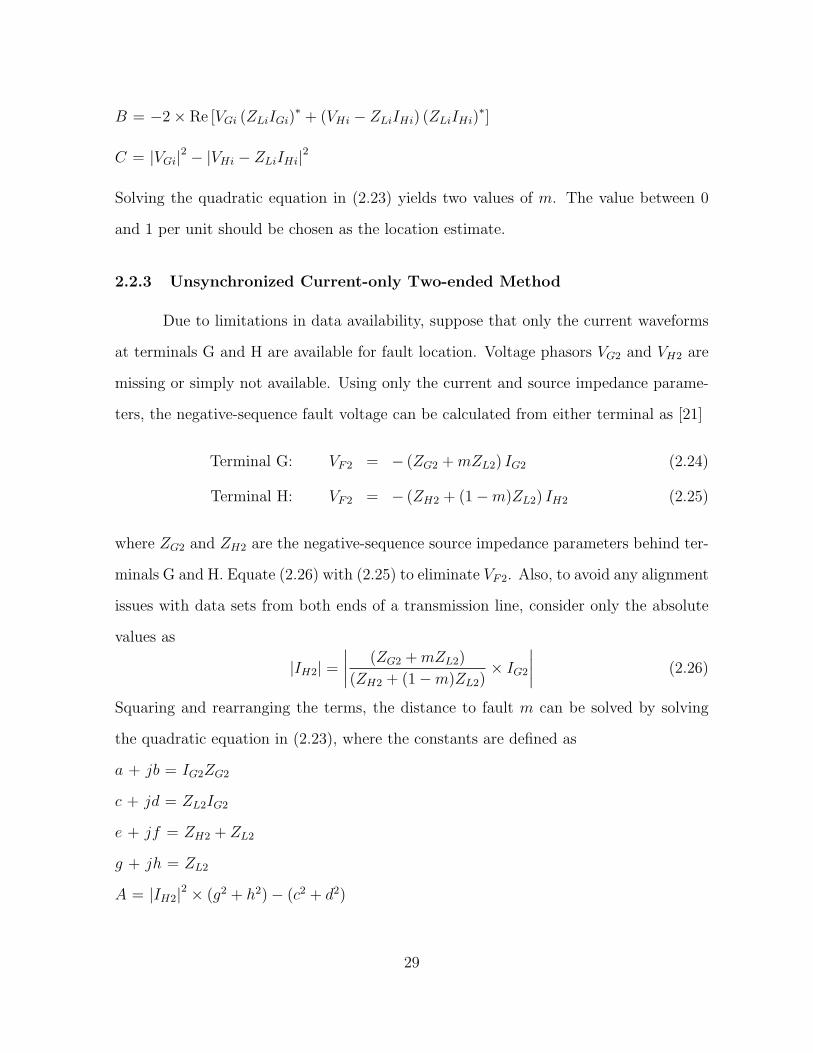
B = −2× Re [VGi (ZLiIGi)∗ + (VHi − ZLiIHi) (ZLiIHi)

∗]

C = |VGi|2 − |VHi − ZLiIHi|2

Solving the quadratic equation in (2.23) yields two values of m. The value between 0

and 1 per unit should be chosen as the location estimate.

2.2.3 Unsynchronized Current-only Two-ended Method

Due to limitations in data availability, suppose that only the current waveforms

at terminals G and H are available for fault location. Voltage phasors VG2 and VH2 are

missing or simply not available. Using only the current and source impedance parame-

ters, the negative-sequence fault voltage can be calculated from either terminal as [21]

Terminal G: VF2 = − (ZG2 +mZL2) IG2 (2.24)

Terminal H: VF2 = − (ZH2 + (1−m)ZL2) IH2 (2.25)

where ZG2 and ZH2 are the negative-sequence source impedance parameters behind ter-

minals G and H. Equate (2.26) with (2.25) to eliminate VF2. Also, to avoid any alignment

issues with data sets from both ends of a transmission line, consider only the absolute

values as

|IH2| =∣

∣

∣

∣

(ZG2 +mZL2)

(ZH2 + (1−m)ZL2)× IG2

∣

∣

∣

∣

(2.26)

Squaring and rearranging the terms, the distance to fault m can be solved by solving

the quadratic equation in (2.23), where the constants are defined as

a + jb = IG2ZG2

c + jd = ZL2IG2

e + jf = ZH2 + ZL2

g + jh = ZL2

A = |IH2|2 × (g2 + h2)− (c2 + d2)

29

B = −2× |IH2|2 (eg + fh)− 2 (ac+ bd)

C = |IH2|2 × (e2 + f 2)− (a2 + b2)

The value of m that lies between 0 and 1 per unit should be chosen as the final location

estimate. This method is applicable for locating unbalanced faults only. Furthermore,

the accuracy of location estimates depends on accurately knowing the source impedance

parameters.

2.3 Summary

This Chapter presents the theory of one- and two-ended impedance-based fault

location algorithms. The input data requirement of each algorithm is summarized in

Table 2.2.

30

Table 2.2: Summary of Input Data Requirements of Impedance-based Fault Location Algorithms

Input DataSimple

ReactanceTakagi

ModifiedTakagi

ErikssonNovoselet al.

SynchronizedTwo-ended

UnsynchronizedTwo-ended

UnsynchronizedCurrent-onlyTwo-ended

Fault Event Data

Fault Type X X X X X

Fault Voltage1

(Local End)X X X X X X X

Fault Current(Local End)

X X X X X X X X

Fault Voltage1

(Remote End)X X

Fault Current(Remote End)

X X X

Synchronized Data X

Prefault Current X X X

Prefault Voltage X

Line Parameters

Line Length X X X X X X X X

Positive-sequenceLine Impedance

X X X X X X X X

Zero-sequenceLine Impedance

X X X X X

Source Impedance Parameters

Positive-sequenceSource Impedance(Local End)

Optional Optional

Positive-sequenceSource Impedance(Remote End)

X

Negative-sequenceSource Impedance(Local End)

X

Negative-sequenceSource Impedance(Remote End)

X

Zero-sequenceSource Impedance(Local End)

Optional

Zero-sequenceSource Impedance(Remote End)

X

1 Voltages measured between the line and the ground.

31

Chapter 3

Error Analysis of Impedance-based Fault Location

Impedance-based fault location algorithms described in Chapter 2 make certain

simplifying assumptions when computing the distance to a fault. Accuracy is affected

when these assumptions do not hold true because of load, fault resistance, current infeed

from a remote source, zero-sequence mutual coupling in parallel lines to name a few. In

addition, impedance-based fault-locating algorithms require the input of the voltage and

current phasors during a fault, and line impedance parameters when estimating the fault

location. Inaccuracy in the input parameters further adds to the error in fault location.

Three-terminal and tapped radial lines can also challenge the application of impedance-

based algorithms. Therefore, the objective of this Chapter is to evaluate the sensitivity

of fault-locating algorithms to the error sources mentioned above. The contribution

lies in using simulation test systems and field data to perform a thorough error analysis

and to gauge the significance of each error source.

Publications:



pp. 537-557, 2014.

– S. Das, S. Santoso, R. Horton, A. Gaikwad, “Effect of earth current return

model on transmission line fault location - a case study,” in Proc. IEEE

Power Energy Soc. General Meeting, Jul. 2013, pp. 1-6.

32

– J. Traphoner, S. Das, S. Santoso, and A. Gaikwad, “Impact of grounded

shield wire assumption on impedance-based fault location algorithms,” in

Proc. IEEE PES General Meeting Conf. Expo., Jul. 2014, pp. 1-5.

– N. Karnik, S. Das, S. Kulkarni, and S. Santoso, “Effect of load current on

fault location estimates of impedance-based methods,” in Proc. IEEE Power

Energy Soc. General Meeting, San Diego, CA, Jul. 2011, pp. 1-6.

– S. Kulkarni, N. Karnik, S. Das, and S. Santoso, “Fault location using impedance-

based algorithms on non-homogeneous feeders,” in Proc. IEEE Power Energy

Soc. General Meeting, San Diego, CA, Jul. 2011, pp. 1-6.

3.1 Benchmark Test Case

To evaluate the sensitivity of impedance-based fault location algorithms to vari-

ous sources of fault-locating error, a two-terminal transmission network shown in Fig. 2.1

was modeled in PSCAD simulation software [47]. The model will be used to replicate ac-

tual short-circuit faults that occur on a transmission line and generate the corresponding

voltage and current waveforms. The rated voltage at terminals G and H is 69 kV. Re-

lays, present at both terminals for line protection, record the three-phase line-to-ground

voltages and currents at 128 samples per cycle. The network upstream from terminal

G is represented by an ideal voltage source EG=1∠10 per unit behind an equivalent

positive- and zero-sequence impedance of ZG1=3.75∠71Ω and ZG0=11.25∠65Ω, re-

spectively. The network upstream from terminal H is also represented by an ideal voltage

source EH =1∠0 per unit behind an equivalent positive- and zero-sequence impedance

of ZH1=12∠71Ω and ZH0=30∠65Ω, respectively. The angle by which EG leads EH

is known as the power angle, δ, and represents the net load served by the transmission

line. The transmission line connecting terminals G and H is 18 miles long and was

modeled using the frequency dependent model in PSCAD. The tower configuration of

33

A

S1

89.25'

80'

15.5' 15.5'

8.75' 8.75'

S2

B C

Figure 3.1: Tower configuration of an actual 69-kV transmission line.

an actual 69-kV transmission line was used as shown in Fig. 3.1. Shield wires S1 and S2

protect phase conductors A, B, and C from direct lightning strikes. The material used to

build the conductors is described in Table 3.1. Using modified Carson’s model [3] and an

earth resistivity value of 100 Ωm, the positive- and zero-sequence line impedances were

calculated to be ZL1=15.55∠69.9Ω and ZL0=35.46∠63.4Ω, respectively. Details on

how to solve line constants have been described in Appendix A.

Note that the test feeder has been intentionally designed to be simple, homoge-

neous, and compliant with all the assumptions made by impedance-based fault location

algorithms. The goal is to introduce the fault-locating error sources one by one and study

the impact on fault location estimates. Since a simple test system is being used, the

error in location estimates is strictly proportional to the inaccuracies introduced. The

analysis will, therefore, give an accurate measure of how significant a particular error

source is and whether the error source should be considered for fault location purposes.

34

Table 3.1: Conductor Data

MaterialResistance Diameter GMR

(Ω/mi) (inch) (feet)

Phase ACSR Linnet 336,400 26/7 0.294 0.720 0.024Shield ACSR Grouse 80,000 8/1 1.404 0.367 0.009

3.2 Fault Location Error due to Inaccurate Input Data

Impedance-based fault location algorithms require the input of fundamental fre-

quency fault voltage and current phasors to calculate the distance to a fault. Unfor-

tunately, because of DC offset and CT saturation, fault current phasors may not be

accurate and will result in a substantial error in location estimates. A delta-connected

potential transformer can introduce error in the calculation of the fault voltage phasor.

In addition, all impedance-based fault location algorithms estimate the impedance to

fault in ohms. Line impedance parameters in ohms per unit distance are required to

obtain a corresponding distance estimate. Uncertainty about these line parameters, par-

ticularly the zero-sequence line impedance further adds to the error in location estimates.

This Section discusses these factors and their impact on fault location accuracy in details.

3.2.1 Inaccurate Current Phasor: DC Offset and CT Saturation

Impedance-based fault location algorithms employ phasor quantities of voltage

and current to compute the distance to a fault. The calculation of these phasor quantities

are complicated by the presence of an exponentially decaying DC offset which makes

the fault current asymmetrical during the first few cycles as shown in Fig. 3.2. The

asymmetry is maximum when a fault occurs at the zero-crossing of a voltage waveform

and minimum when a fault occurs near the voltage peak. Fortunately, most single line-to-

ground faults are caused by an animal or a tree coming into contact with a transmission

line during peak voltage conditions [7]. In such cases, the DC offset is negligible. Faults

35

Figure 3.2: Fault current with a significant DC offset.

due to lightning strikes are, however, random and can occur at any point on the voltage

waveform, resulting in a significant asymmetry in the fault current.

To filter out the decaying DC offset and calculate the fault current phasor, Fast

Fourier transforms (FFT) are commonly used [14]. A window length of one cycle is

used to extract the fundamental-frequency magnitude and phase angle, and discard all

harmonics. As an example, a rolling FFT filter is applied to the waveform in Fig. 3.2. In

a rolling FFT, the FFT operation is performed repeatedly by a one-cycle long window

sweeping across the entire waveform. Figure 3.3 shows that the FFT operation is suc-

cessful in filtering out most, but not all of the DC offset. The fault current magnitude

fluctuates and reaches steady-state only when the DC offset decays. The corresponding

variation in location estimates from the simple reactance method is shown in Fig. 3.4.

The cosine filter is another phasor estimation technique commonly used in Schweitzer

relays [62]. The coefficients of this filter are sampled from a cosine wave and require

36

2 4 6 8 10 12 14 160

1

2

3

4

5

6

7

8

9

Cycles

IA R

MS

Mag

nitu

de (

kA)

Cosine FilterFFT FilterNote the response

of the FFT Filter

Figure 3.3: Cosine filter is more effective in filtering out the DC offset than the FFTfilter.

a minimum response time of one and a quarter cycles. The quarter-cycle delay is used

to calculate the phase angle. As seen in Fig. 3.3, the cosine filter does a better job of

eliminating the DC offset than the FFT filter. The front and tail end of the signal are,

however, severely distorted. This distortion can offset the accuracy of fault current pha-

sor calculation during short-duration faults, resulting in erroneous location estimates.

In addition to DC offset, saturation of a current transformer (CT) can also dis-

tort the fault current waveforms and introduce a significant error in location estimates.

CT saturation is often caused by fault currents having a significant DC offset [7]. As

the DC offset decays down within two or three cycles, the saturated CT may return to

normal operating conditions. Therefore, for faults that last for a number of cycles, the

best way to handle CT saturation is to wait for the DC offset to decay before applying

37

0 1 2 3 43.8

3.9

4

4.1

4.2

4.3

4.4

4.5

4.6

4.7

Cycles

Dis

tanc

e T

o F

ault

Est

imat

e (m

i)

Simple Reactance Method

Figure 3.4: Variation in location estimates from the simple reactance method due to DCOffset. Voltage and current phasors were calculated using the FFT filter.

fault location algorithms.

3.2.2 Inaccurate Voltage Phasor: Delta-connected Potential Transformer

Impedance-based fault location algorithms require the input of line-to-ground

voltages when computing the distance to a fault. When potential transformers are

connected in a delta configuration, line-to-line voltages are available instead. The mea-

sured line-to-line voltages can be used by one-ended algorithms to estimate the location

of line-to-line, double line-to-ground, or three-phase faults with no loss in accuracy.

Line-to-ground voltages are, however, necessary to estimate the location of single line-

to-ground faults [15]. If the zero-sequence impedance of the source, ZGO, is available,

then the line-to-ground voltage during a A-G fault can be estimated as

VAF =1

3(VAB − VCA)− ZG0IG0 (3.1)

38

where VAF is the estimated line-to-ground voltage of the faulted phase (phase A), VAB

is the line-to-line fault voltage measured between phases A and B, and VCA is the line-

to-line fault voltage measured between phases C and A. Accuracy of the estimated line-

to-ground fault voltage depends on the accuracy of the zero-sequence source impedance.

3.2.3 Inaccurate Line Parameters: Untransposed Lines

Impedance-based fault location algorithms require the positive- and zero-sequence

impedances of a transmission line to estimate the distance to a fault. When calculat-

ing the sequence line parameters, transmission lines are assumed to be transposed as

explained in Appendix A. Transposition is the principle of physically exchanging the po-

sition of phase conductors at periodic intervals such that a particular conductor occupies

all positions of a particular line configuration. This principle is illustrated in Fig. 3.5,

where the positions of phase conductors A, B, and C are rotated every one-third of the

total line length. Transposition equalizes the mutual coupling between the three phases

and reduces the sequence impedance matrix, Z012, to a diagonal matrix as shown in

(3.2). The diagonal elements are formed by the sequence line impedances while the

off-diagonal elements are zero, indicating no coupling between the sequence networks.

Z012 =

ZL0 0 00 ZL1 00 0 ZL2

Ω (3.2)

Although transposing a line is advantageous, it introduces complications in the

design of a transmission line, and increases the overall design cost due to additional sup-

port structures and insulator string requirements. As a result, many transmission lines

are not transposed. The sequence impedance matrix of an 18-mile long untransposed

line having the same line configuration shown in Fig. 3.1 is:

Z012 =

15.47 + j32.52 0.26 + j0.00 0.26 + j0.000.26 + j0.00 5.33 + j15.15 0.00− j1.020.26 + j0.00 0.00− j1.02 5.33 + j15.15

Ω

39

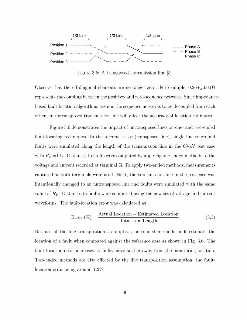
1/3 Line 1/3 Line 1/3 Line

Phase APhase BPhase C

Position 3

Position 2

Position 1

Figure 3.5: A transposed transmission line [5].

Observe that the off-diagonal elements are no longer zero. For example, 0.26+j0.00Ω

represents the coupling between the positive- and zero-sequence network. Since impedance-

based fault location algorithms assume the sequence networks to be decoupled from each

other, an untransposed transmission line will affect the accuracy of location estimates.

Figure 3.6 demonstrates the impact of untransposed lines on one- and two-ended

fault-locating techniques. In the reference case (transposed line), single line-to-ground

faults were simulated along the length of the transmission line in the 69-kV test case

with RF =0Ω. Distances to faults were computed by applying one-ended methods to the

voltage and current recorded at terminal G. To apply two-ended methods, measurements

captured at both terminals were used. Next, the transmission line in the test case was

intentionally changed to an untransposed line and faults were simulated with the same

value of RF . Distances to faults were computed using the new set of voltage and current

waveforms. The fault-location error was calculated as

Error (%) =Actual Location− Estimated Location

Total Line Length(3.3)

Because of the line transposition assumption, one-ended methods underestimate the

location of a fault when compared against the reference case as shown in Fig. 3.6. The

fault-location error increases as faults move farther away from the monitoring location.

Two-ended methods are also affected by the line transposition assumption, the fault-

location error being around 1.2%.

40

Figure 3.6: Error in fault location due to untransposed transmission lines.

3.2.4 Inaccurate Line Parameters: Uncertainty in Earth Resistivity

Earth resistivity ρ is the resistance with which the earth opposes the flow of

electric current. It is an electrical characteristic of the ground and plays a critical role

when calculating the zero-sequence impedance of a transmission line [3]. Determining

the exact value of ρ is difficult since it varies greatly with the soil type as shown in

Table 3.2. Most utilities use a standard earth resistivity value of 100 Ωm while others

use the Wenner four-point method to measure ρ with great accuracy [43]. In addition

to soil type, the value of ρ is also dictated by the moisture content in soils, temperature,

and season of the year. Under extremely high or low temperatures, the soil is dry and

41

Table 3.2: Variation of Earth Resistivity with Soil Type [1]

Soil TypeEarth Resistivity (Ωm)

Range Average

Peat >1200 200Adobe clay 2-200 40Boggy ground 2-50 30Gravel (moist) 50-3000 1000 (moist)Sand and sandy ground 50-3000 200 (moist)Stony and rocky ground 100-8000 2000Concrete: 1 part cement + 3 parts sand 50-300 150

Table 3.3: Effect of Earth Resistivity on Line Impedance Parameters

ρincreases

y

ρ (Ωm) ZL1 (Ω) ZL0 (Ω)

10 5.33 + j15.15 13.59 + j30.34100 5.33 + j15.15 15.47 + j32.53500 5.33 + j15.15 16.74 + j33.871000 5.33 + j15.15 17.28 + j34.40

y

ZL0increases

has a very high earth resistivity value. During the rainy season, the value of ρ decreases.

Minerals, salts, and other electrolytes make soils more conductive and tend to lower the

earth resistivity value. Put another way, earth resistivity is never constant and is never

known accurately. Table 3.3 shows the impact of a varying earth resistivity value on

the positive- and zero-sequence impedances of the 69-kV transmission line described in

Section 3.1. The positive-sequence line impedance remains unaffected by changes in the

value of earth resistivity. The zero-sequence line impedance, on the other hand, increases

as ρ increases. Since one-ended fault location algorithms require the zero-sequence line

impedance to compute the location of single line-to-ground faults, these methods are

sensitive to any changes in earth resistivity.

As an example, the 69-kV test case was used to demonstrate the detrimental

effect of ρ on one-ended methods. Single line-to-ground faults were simulated along the

42

Figure 3.7: Error in fault location due to uncertainty in earth resistivity.

entire length of the transmission line with earth resistivity values ranging from 10 to

1000 Ωm. Line impedance parameters, used as an input to the fault location algorithms,

were, however, calculated using the standard earth resistivity value of 100 Ωm. This case

study reflects a practical scenario in which the resistivity of the soil can indeed vary over

such a wide range. However, line impedance settings in a digital relay or a fault locator

are computed using a particular value of ρ and do not reflect that change. As expected,

the accuracy of one-ended methods are affected by the uncertainty in earth resistivity as

shown in Fig. 3.7. When the actual value of earth resistivity is greater than the one used

in the fault location computation, i.e., 100 Ωm, the distance to fault is overestimated.

43

Similarly, when ρ is lower than the value used in the fault location computation, the

distance to fault is underestimated. Also observe that the fault-location error increases

linearly as the fault moves farther away from the monitoring location. This is because the

error due to inaccurate zero-sequence line impedance adds up as the line length between

the monitoring location and the fault increases. In contrast, two-ended methods do not

use zero-sequence line impedance when estimating the distance to fault and are hence,

not affected by any variation in earth resistivity.

3.2.5 Inaccurate Line Parameters: Tower Footing Resistance

When calculating the phase impedance matrix of the transmission line, the neu-

tral conductor is assumed to be perfectly grounded to the earth as described in Ap-

pendix A. In practice, shield wires are grounded to the earth through a finite tower

footing resistance which has a value between 25 and 100 ohms as illustrated in Fig. 3.8.

In the figure, span is the length of the transmission line between two adjacent towers

and RT is the tower footing resistance. The network formed by the shield wire and tower

footing resistance is shown in Fig. 3.9 where Znn is the self-impedance of the earth wire

per span. Since the neutral is no longer at earth potential, line impedance calculated

using Kron reduction will be different from the actual line impedance and will affect the

accuracy of fault location estimates.

To analyze the impact of tower footing resistance on the accuracy of impedance-

based fault location algorithms, the test case described in Section 3.1 was used with

certain additional modifications. The transmission line is 3.73 miles long and supported

by transmission towers every 1000 feet as shown in Fig. 3.10. Arrangement of the phase

and neutral conductors, and conductor material remain the same as those given by

Fig. 3.1 and Table 3.1. Since the objective is to investigate the effect of tower grounding

resistances on the accuracy of fault location algorithms, the transmission line is built as

44

Figure 3.8: Shield wire grounded through tower footing resistances, RT [6].

znn

RT

znn znn

RTRT

znnShield Wire

Figure 3.9: Network of the tower footing resistance and the shield wire impedance.

an n-phase model with a detailed representation of tower footing resistances as shown

in Fig. 3.11. Note that in an n-phase model, all conductors are modeled explicitly in the

simulation model. For example, in a three-phase system with two neutral conductors,

the n-phase model will be modeled as a 5-conductor system.

Next, single line-to-ground faults were simulated at 0.75 mi, 1.86 mi, and 2.80

mi from the monitor. For each fault, the tower footing resistance at every tower was

varied at the following values: 0Ω, 5Ω, and 20Ω. The goal was to investigate whether

the magnitude of the tower footing resistance and the number of towers between the

monitor and the fault play a significant role in the fault location accuracy. As seen in

45

3.73 miTerminal G

VG,IG

ZG

VH,IH

Terminal H

ZH

EGEH

1000 ft

Figure 3.10: Transmission line of benchmark test case reduced to 3.73 miles and sup-ported by towers every 1000 feet.

Figure 3.11: Transmission line modeled as an n-phase model in PSCAD with the twoshield wires, S1 and S2, grounded through a tower footing resistance RT .

Table 3.4, when the tower footing resistance is 0 Ω, estimates from the Eriksson method

are accurate. However, for non-zero values of tower footing resistance, the fault location

error increases. The percent error depends on how far the fault is from the monitor

rather than on the magnitude of the tower footing resistance.

Fault location error from the one-ended methods can be explained by the fact

that the tower footing resistance affects the value of the zero-sequence line impedance

as shown in Fig. 3.5. The positive-sequence impedance of the line remains unchanged.

46

Figure 3.12: The impedance scan block in PSCAD was used to calculate the zero-sequence line impedance at different tower footing resistance values.

It should be noted that the impedance scan function block in PSCAD [47] was used to

calculate the sequence line impedances at different values of tower footing resistance.

This block is a powerful feature of PSCAD and generates the equivalent impedance

matrix as seen from the interface point as shown in Fig. 3.12.

Distance to fault estimates from the two-ended unsynchronized negative-sequence

method are shown in Table 3.6. Accuracy of this method is not affected by the presence

of the tower footing resistance. This is because two-ended methods do not use zero-

sequence line impedance in their fault location computation.

From the analysis described above, it can be concluded that the tower footing

resistance affects the magnitude of the zero-sequence line impedance. Because the zero-

sequence line impedance is required by one-ended methods to locate single line-to-ground

faults, the accuracy of these methods are affected by the tower footing resistance. The

increase in error is, however, marginal, around 4%. The analysis also concludes that

the size of the tower footing resistance and the number of towers between the monitor

and the fault have a negligible impact on one-ended methods. In contrast, two-ended

methods are robust to the presence of the tower footing resistance.

47

Table 3.4: Impact of RT on the Eriksson Method

Actual Location

(mi)

Estimated Location (mi)

RT =0 Ω RT =5 Ω RT =20 Ω

0.75 0.74 0.78 0.78

1.86 1.85 1.96 1.96

2.80 2.78 2.94 2.95

Table 3.5: Effect of RT on the Positive- and Zero-sequence Line Impedances

RT =0 Ω RT =5 Ω RT =20 Ω

Zero-sequence Line Impedance (Ω) 9.50∠70.8 10.02∠78.3 10.03∠78.5

Positive-sequence Line Impedance (Ω) 3.25∠73.0 3.25∠73.0 3.25∠73.0

Table 3.6: Impact of RT on the Unsynchronized Two-ended Method

Actual Location

(mi)


RT =0 Ω RT =5 Ω RT =20 Ω

0.75 0.75 0.75 0.75

1.86 1.86 1.86 1.86

2.80 2.80 2.80 2.80

3.2.6 Inaccurate Line Parameters: Earth Current Return Model

Transmission networks are not perfectly balanced due to untransposed lines,

loads, and unbalanced faults. As a result, the residual current, which is the summation

48

of currents in all the three phases, flows back to the source through the neutral. Since

transmission lines are multi-grounded systems, i.e., the neutral conductor is grounded

at multiple points along the length of a transmission line, this return current is shared

between the earth and neutral [63]. The current through the earth cannot penetrate

deep into the ground due to a condition similar to skin effect [64]. Instead, they flow

along the surface just underneath the conductor as shown in Fig. 3.13.

V0

I0

Ia

Ic

Ib

In

Earth

Figure 3.13: Earth current return in a three-phase four wire multi-grounded system [7].

To account for earth current return, three well known modeling methods are Full

Carson’s model, modified Carson’s model, and Deri model. Equations governing each

model are described in Appendix A. The motivation for the study stems from the fact

that line constants calculated using each of the three models are not exactly identical.

For example, Table 3.7 shows the line impedances of the transmission line in Fig. 9.19,

solved using the different earth current return models at an earth resistivity value of 100

Ω-m. The positive-sequence line impedance from all the three models match relatively

well. This is because the positive-sequence currents do not flow through the earth and

is, hence, not affected by the earth model. The zero-sequence impedance, particularly

49

Table 3.7: Line Parameters using Different Earth Current Return Models

Earth Return Model ZL1 (Ω/mi) ZL0 (Ω/mi)

Full Carson’s Model 6.01+ j19.00 19.72+ j56.23

Modified Carson’s Model 6.01+ j19.00 19.82+ j55.93

Deri Model 5.92+ j19.00 19.95+ j56.53

the zero-sequence reactance, show minor differences. Since transmission lines travel

over wide geographical distances, seemingly minor differences in line constant values can

affect the accuracy of fault location estimates.

To investigate how line constants calculated using different earth return models

affect the accuracy of impedance-based fault location algorithms, actual fault event

data described in Section 9.4 was used. Using actual fault data is advantageous since

no assumptions about the earth need to be made. Results are, therefore, not biased.

The approach consists of using line constants, calculated using each of the three earth

models, as an input to the Takagi method. As observed from Table 3.8, estimates using

each of the three modeling methods yield almost identical results and are close to the

actual location of the fault. Also note that the results are not consistent for the same

fault event. For example, for events 1 and 2, the modified Carson’s model yields location

estimates that are close to the actual fault location. In events 3 and 4, on the other

hand, Deri model is more accurate. The inconsistency is due to other factors such as

DC offset which influence the accuracy of location estimates. Therefore, the analysis

concludes that any of the three earth modeling techniques can be used for fault location

computation without any significant variation in accuracy.

50

Table 3.8: Fault Location Estimates using Line Parameters Computed by Different EarthReturn Models

Event Earth Return ModelFault Location (mi)

Estimated Actual

Event 1 Full Carson’s Model 14.20

14.37

1/10/2012 Modified Carson’s Model 14.2412:44:38.413 Deri Model 14.15

Event 2 Full Carson’s Model 14.071/10/2012 Modified Carson’s Model 14.1212:44:38.897 Deri Model 14.03



3.2.7 Inaccurate Line Parameters: Non-homogeneous Lines

Both one- and two-ended impedance-based fault location algorithms assume a

homogeneous overhead feeder with a uniform impedance per unit mile. However, prac-

tical utility distribution feeders are constructed using different conductor types and pole

configurations. As an example, a 7.6-mile long utility circuit can be constructed as fol-

lows: 0.13 miles using 2-ACSR phase and neutral conductors, 1.25 miles using 336-AAC

phase and 1/0-ACSR neutral conductors, and 6.23 miles using 556-AAC phase and 336-

AAC neutral conductors. Such a non-homogeneous feeder can affect the accuracy of

impedance-based fault location algorithms. A comprehensive analysis conducted in [55]

concludes that the fault location accuracy in non-homogeneous feeders may be preserved

by using the line impedance parameters of the most commonly occurring line conductor.

In this example, this means using the positive- and zero-sequence line impedances of the

556-AAC phase and 336-AAC neutral configuration.

51

3.3 Fault Location Error due to Application Challenges

Impedance-based fault location techniques described in Chapter 2 make certain

simplifying assumptions. The accuracies of location estimates are compromised when

these assumptions do not hold true because of load, non-homogeneous system, and

double-circuit transmission lines. The task of locating faults is further complicated by

tapped radial lines or three-terminal transmission networks. The objective of this Section

is to evaluate the error in fault location due to such application related challenges.

3.3.1 System Load

This Section investigates the impact of system load on the accuracy of impedance-

based fault location algorithms. System load as an error source is particularly dominant

in distribution feeders. To conduct the analysis, the 69-kV case was used to simulate

single line-to-ground faults at several locations of the 18-mile long transmission line with

different values of δ and RF . Recall that δ represents the net load served by the trans-

mission network. One-ended fault location algorithms use voltage and current captured

at terminal G while two-ended algorithms use waveforms captured at both line ends.

When the fault resistance is zero, location estimates from the simple reactance

method are accurate, even under heavily loaded conditions as shown in Fig. 3.14. Note

that a power angle of 20 corresponds to a load current of 430A. For non-zero values of

fault resistance, however, the same values of load current cause a reactance error in the

simple reactance method. The reactance error is capacitive and the simple reactance

method underestimates the location of faults. The fault-location error is further magni-

fied when the load and fault resistance is increased to 40 and 15Ω, respectively. It is also

interesting to observe the increase in reactance error as the distance to fault increases in

Fig. 3.14. When faults occur towards the end of the transmission line, the fault current

contribution from the local terminal decreases. The load current constitutes a significant

52

0 0.2 0.4 0.6 0.8 1−40

−35

−30

−25

−20

−15

−10

−5

0

5

10

Distance to Fault (pu)

Fau

lt Lo

catio

n E

rror

(%

)

Simple Reactance Method

ρ = 20°, RF = 0 Ω

ρ = 20°, RF = 5 Ω

ρ = 20°, RF = 10 Ω

ρ = 40°, RF = 15 Ω

Reference Case

Figure 3.14: Reactance error due to load in the simple reactance method.

0 0.2 0.4 0.6 0.8 1

-0.25

-0.2

-0.15

-0.1

-0.05

0

0.05

0.1

0.15

0.2

0.25

Distance to Fault (pu)

Fau

lt Lo

catio

n E

rror

(%

)

20 Degree Load, Fault Resistance 10 Ω

TakagiErikssonModified Takagi,Two-ended

Figure 3.15: Load has no impact on the Takagi, Modified Takagi, Eriksson, and Two-ended methods.

53

percent of the total fault current and increases the phase angle mismatch between IF and

IG. For example, when a fault occurs at 0.8 per unit from terminal G, the load current is

28% of the fault current recorded at terminal G. As a result, the reactance error increases.

Takagi method uses the “pure fault” current to minimize the reactance error due

to load. As shown in Fig. 3.15, the reactance error is negligible when RF =10Ω and

δ=20. Modified Takagi, Eriksson, and two-ended methods are also not affected by an

increase in the system load.

3.3.2 Non-homogeneous System

To demonstrate the effect of a non-homogeneous system on impedance-based

fault location algorithms, the 69-kV benchmark test case was used. The test case is

homogeneous since the local and remote source impedances have the same angle as the

line impedance and hence, serves as the reference case. Single line-to-ground faults were

simulated along the entire length of the transmission line with δ=1 and RF =5Ω. To

compute the location of faults, one-ended methods use voltage and current waveforms

at terminal G while two-ended methods use voltage and current measurements at both

terminals. Next, the system is intentionally made non-homogeneous by changing the

value of ZG1 to 15∠50Ω. Faults were simulated using the same values of fault resistance

and load. Location estimates from one and two-ended methods, computed using the

new set of voltage and current measurements, were compared with those obtained in the

reference case (homogeneous system) as shown in Fig. 3.16. As expected, the accuracy

of simple reactance and Takagi methods deteriorate in a non-homogeneous system. The

Eriksson method uses the remote source impedance to improve upon the performance

of the Takagi method. The modified Takagi and two-ended methods are also robust to

the increase in non-homogeneity and remain unaffected.

54

Figure 3.16: Effect of a non-homogeneous system on impedance-based fault locationalgorithms.

3.3.3 Parallel Lines

In transmission networks, it is common to find transmission lines that are physi-

cally parallel to each other. Two three-phase lines may be supported by the same tower

or they may run on two separate towers but share the same right of way. Because of

the mutual coupling between two lines, the impedance to fault calculation is influenced

by currents flowing in the parallel line, thereby compromising the accuracy of location

estimates. As an example, consider the double-circuit transmission network shown in

Fig. 3.17. The rated voltage at terminals G and H is 69 kV. Source impedance param-

eters ZG and ZH have the same values as those used in Section 3.1. The transmission

line is 18 miles long and has the configuration of an actual 69-kV double-circuit trans-

mission line as shown in Fig. 3.18. Phase conductors A, B, and C represent Line 1 in

Fig. 3.17 while phase conductors A’, B’, and C’ represent Line 2. Materials used to build

55

Figure 3.17: Double-circuit transmission network.

the conductors are the same as those described in Table 3.1. Assuming both lines to

be completely transposed and using an earth resistivity value of 100 Ωm, the sequence

impedance matrix Z012 of the transmission line is given as

Z012 =

15.82 + j40.91 0 0 10.52 + j25.77 0 00 5.33 + j12.92 0 0 0 00 0 5.33 + j12.92 0 0 0

10.52 + j25.77 0 0 15.82 + j40.91 0 00 0 0 0 5.33 + j12.92 00 0 0 0 0 5.33 + j12.92

Ω

Here, the off-diagonal term 10.52+ j25.77 Ω represents the zero-sequence mutual cou-

pling (Z0M) between two parallel lines and will always be present, regardless of whether

the line is transposed or not. Observe that Z0M is significant, around 63% of the zero-

sequence line impedance. Because of Z0M , the apparent impedance measured at terminal

G during a fault on Line 2 changes and can be written as

Zapp =VG

IG= mZL1 +mZ0M

(

IJ0IG

)

+RF

(

IFIG

)

(3.4)

where IJ0 is the zero-sequence current in the parallel transmission line. If the two

lines are parallel to each other for the entire line length, then Z0M can be taken into

consideration by simply measuring IJ0 and inputting the value to (3.4). However, many

different configurations of parallel lines are possible. For example, two lines may start

parallel to each other from one terminal but end at two different terminals [65]. In such

cases, the term mZ0M (IJ0/IG) will affect the accuracy of distance-to-fault estimates.

56

A

S

7'

50'

5'

B

C C’

B’

A’

7'

5'

5'

Figure 3.18: Configuration of an actual 69-kV double-circuit transmission line.

If current IG flows in the same direction as the current in the parallel line, IJ , then

one-ended fault locating techniques will overestimate the location of the fault. On the

other hand, if currents IG and IJ flow in opposite directions, one-ended methods will

underestimate the location of the fault [13].

To evaluate the impact of ZOM on impedance-based fault location algorithms, the

test case described in Fig. 3.17 was used. Analysis begins by first developing a reference

case wherein there is no zero-sequence mutual coupling between the two lines. In reality,

this is possible only when the two parallel lines are far apart from each other. Single line-

to-ground faults were simulated at various locations of Line 2 with RF =0Ω and a load

angle of δ=10. To compute the location of faults, one-ended methods use the voltage

and current waveforms at terminal G while two-ended methods use waveforms at both

ends of the line. Next, Z0M was intentionally introduced in the base case and the same

57

Figure 3.19: Impact of zero-sequence mutual coupling on impedance-based fault locationalgorithms.

faults were simulated on Line 2. Location estimates computed using the new waveforms

were then compared with those obtained in the reference case to obtain the increase in

fault-locating error due to Z0M . As shown in Fig. 3.19, all one-ended methods are equally

affected by Z0M . The increase in fault-locating error is around 10% at the far end of the

line. Note that in this analysis, Z0M was not compensated by IJ0 in the parallel line.

The two-ended synchronized or the two-ended unsynchronized methods do not

use the zero-sequence network when computing the distance to a fault. As a result,

they are not affected by Z0M as shown in Fig. 3.19. The unsynchronized current-only

58

two-ended method is also not affected by Z0M . However, this method does require the

knowledge of negative-sequence currents IJ2 and IK2 flowing in the parallel transmission

line. This is because IJ2 and IK2 cause an additional voltage drop across the source

impedances ZG and ZH and if neglected, will cause an error in the location estimates.

Recall from Section 2.2.3 that the unsynchronized current-only two-ended method solves

for the distance to fault m by the quadratic equation given in (2.23). For double circuit

lines, constants a and b change and are defined as follows:

a+ jb = IG2ZG2 + IJ2ZG2 − IK2ZH2

The other constants remain the same. The unsynchronized current-only two-ended

method is not affected by the different configurations of parallel transmission lines.

3.3.4 Three-terminal Lines

Impedance-based fault location algorithms in Chapter 2 have been primarily de-

veloped for a two-terminal transmission line and can be extended to locate faults on

a radial distribution feeder. However, the application scenario changes in the case of

a three-terminal line as shown in Fig. 3.20. One-ended fault location algorithms are

accurate up to the tap point only. When a fault occurs beyond the tap point, the fault

current contributed by the third terminal (terminal T) modifies the impedance to fault

equation and results in a significant error in location estimates. For example, consider

the fault shown in Fig. 3.20. The apparent impedance measured from terminal G is:

Zapp =VG

IG= mZL1 + (m−D)ZL1

ITIG

+RF

(

IFIG

)

(3.5)

where IT is the fault current contributed by terminal T and D is the distance of the tap

point from terminal G. Since one-ended algorithms at terminal G have no knowledge

about IT , the term (m−D)ZL1 (IT/IG) will cause one-ended methods to overestimate

the location of the fault. Moreover, current IF is the summation of IG, IH , and IT . As

59

Figure 3.20: Three-terminal transmission line.

a result, IF and IG have different phase angles in a non-homogeneous system and will

introduce an additional reactance error. Depending on whether the reactance error is

inductive or capacitive, distance to fault is over or underestimated. One-ended methods

applied from terminal H, on the other hand, can successfully estimate the location of

fault F. Since the fault is located before the tap point, the fault current contributed by

terminals G and T act as remote infeed only and do not alter the apparent impedance

measured from terminal H. Therefore, the solution in the case of three-terminal lines

is to apply one-ended methods from each terminal. One of the three estimates will

successfully pinpoint the exact location of the fault as demonstrated in the case study

described in Section 3.4.3. Two-ended algorithms can be extended for application to

three-terminal lines with certain additional modifications. For instance, authors in [21]

transform a three-terminal line into an equivalent two-terminal line and then apply the

unsynchronized current-only two-ended method.

3.3.5 Tapped Radial Line

Locating faults on a radial feeder tapped from a two-terminal transmission line is

a challenging task for impedance-based fault location algorithms. When a fault occurs

60

in the line section between the tap point and the load, as illustrated by F in Fig. 3.21,

the apparent impedance measured from terminal G is the same as that given by (3.5).

One-ended algorithms make use of measurements captured at only one end of the line.

Therefore, neglecting the fault current contributed by terminal H will cause one-ended

methods to overestimate the fault location.

Figure 3.21: Fault on a radial feeder tapped from a two-terminal line.

Measurements captured at both ends of a line can be used to improve the accuracy

of location estimates. The first step is to confirm whether the fault is located on the

radial line. This is achieved by calculating the voltage at the tap point during fault,

VTap, from terminals G and H as shown below:

Terminal G: VTap = VG −DZL1IG (3.6)

Terminal H: VTap = VH (3.7)

If the fault is on the radial line, VTap calculated from terminal G will equal that calculated

from terminal H. This is because terminals G and H operate in parallel to feed the fault

on the radial line. Next, (3.5) can be used to compute the distance to fault.

61

3.4 Application of Impedance-based Fault Location Algorithmsto Field Data

This Section demonstrates the application of impedance-based fault location al-

gorithms on actual fault event data captured in utility transmission and distribution

networks. Data consists of voltage and current waveforms recorded by digital relays

and digital fault recorders, line impedance parameters, and known location of the fault.

Each event was chosen to highlight a unique aspect of impedance-based fault location.

3.4.1 Event 1: Lightning Strike on a 161-kV Transmission Line - SuccessfulFault Location from One-ended Methods

On 12 June 2011, a lightning strike caused a line-to-line fault between phases B

and C of a 161-kV transmission line at 1:33 pm. The transmission line is radial and

has a total length of 12.58 miles. The positive- and zero-sequence line impedances are

ZL1=1.38+ j9.32Ω and ZL0=5.88+ j25.86Ω, respectively. According to the utility, the

fault is located 7.54 miles from Station 1 as shown in Fig. 3.22. A digital fault recorder

at Station 1 captures the three-phase line-to-ground voltages and currents during the

fault at 100 samples per cycle as shown in Fig. 3.23. Before the fault, Station 1 supports

a load current of 110A. During the fault, the current magnitude increases to 3.5 kA

in the faulted phases. The fault lasts for three cycles, after which the fault current is

interrupted by the operation of a circuit breaker at Station 1.

To estimate the distance to fault, one-ended fault location algorithms were ap-

plied to the voltage and current waveforms captured at Station 1. Notice that the fault

currents have a significant DC offset. Therefore, to minimize the effect of DC offset,

the third cycle after fault inception was selected for computing the distance to fault

as illustrated in Fig. 3.23. Because the transmission line is radial in nature, Novosel

et al. method was used instead of the Eriksson method. The positive-sequence source

impedance (ZG1), required as an additional input to the Novosel et al. method, was

62

VG,IGStation 1 Fault Point F

7.54 mi 5.05 mi

Load

ZG1, ZG0

Figure 3.22: Event 1 is a BC fault at 7.54 miles from Station 1.

Figure 3.23: Event 1 waveforms captured by the DFR at Station 1.

computed using (8.44) to be 4.03+j20.22Ω. As seen from Table 3.9, location estimates

from one-ended algorithms are in agreement with that estimated by the DFR and are

close to the actual location of the fault. In summary, this event demonstrates the success

of one-ended algorithms in tracking down the exact location of a fault.

63

Table 3.9: Event 1 Fault Location Estimates from One-ended Methods

Station Actual Location DFR EstimateEstimated Location (mi)

(mi) (mi) Simple Reactance Takagi Novosel et al.

1 7.54 7.60 7.34 7.38 7.35

3.4.2 Event 2: Bird Contact with a 161-kV Transmission Line - SuperiorPerformance of Two-ended Methods over One-ended Methods

Event 2 is a single line-to-ground fault event on phase A that occurred on 29

March 2012 at 7:28 pm. The fault was caused by birds coming in contact with a 161-

kV transmission line that connects Station 1 with Station 2 as shown in Fig. 3.24.

The transmission line is 31.30 miles long and has a total positive- and zero-sequence

line impedance of ZL1=5.00+ j25.27 Ω and ZL0=23.67+ j79.40 Ω, respectively. The

actual distance to the fault is known to be 30.86 miles from Station 1 or 0.44 miles from

Station 2 as shown in Fig. 3.24.

Digital fault recorders at Station 1 and Station 2 record the voltage and current

waveforms at 96 samples per cycle. Before the fault, load currents at Station 1 and

Station 2 are 89A and 70A, respectively. During the fault, the circuit breaker at Station

2 measures a fault current magnitude of 5.86 kA and trips in 2.5 cycles as seen from

VG,IGStation 1 Fault Point F

VH,IH Station 2

DFR DFRZG1 ZH1

30.86 mi 0.44 mi

Figure 3.24: Event 2 is a A-G fault 30.86 miles from Station 1 or 0.44 miles from Station2.

64

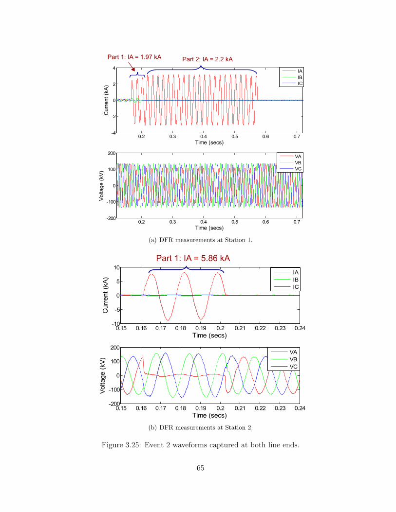
(a) DFR measurements at Station 1.

(b) DFR measurements at Station 2.

Figure 3.25: Event 2 waveforms captured at both line ends.

65

Fig. 3.25(b). Station 1, on the other hand, continues to contribute fault current for 22.5

cycles. During the first 2.5 cycles, when both stations are feeding the fault, the DFR

at Station 1 records a fault current of 1.97 kA as indicated by “Part 1” in Fig. 3.25(a).

After 2.5 cycles, when Station 2 trips offline due to the operation of a circuit breaker,

fault current contributed by Station 1 increases to 2.2 kA as illustrated by “Part 2” in

Fig. 3.25(a).

To compute the location of the fault from Station 1, impedance-based fault lo-

cating algorithms were applied to “Part 2” of the waveform data. This is because in

“Part 2”, only Station 1 contributes current to the fault without remote infeed from

Station 2. As a result, location estimates are expected to be accurate. Unfortunately,

as observed from Table 3.10, the distance to fault estimates are offset from the actual

fault location by 7 miles. In addition to the one-ended methods, the DFR present at

Station 1 also underestimates the location of the fault by 5 miles. Although the source

of error is not apparent, an erroneous estimate from the Eriksson method rules out fault

resistance, non-homogeneous system, and load current as possible sources of error. It

is possible that the zero-sequence line impedance parameter is incorrect and may have

offset the accuracy of location estimates. Distance to fault computed from Station 2

waveforms, on the other hand, are close to the actual location of the fault. Note that

the source impedance parameters, required as an input to the Eriksson method, were

estimated using (8.44) to be ZG1= j11.71Ω and ZH1=0.11+j11.73Ω.

To investigate whether two-ended methods can improve the accuracy of loca-

tion estimates, the unsynchronized current-only two-ended method was chosen since the

DFRs at Station 1 and Station 2 have different fault trigger times. The waveforms are,

therefore, unsynchronized. The two-ended method was applied to that part of the fault

wherein both stations are contributing to the fault, i.e.,“Part 1” of Station 1 and Station

2 waveforms. As seen from Table 3.11, the location estimate from the two-ended method

66

shows a significant improvement over the one-ended methods. Recall that two-ended

methods do not require zero-sequence line impedance in their fault location calculation.

In summary, this event highlights the superior performance of two-ended methods over

one-ended methods in computing the distance to a fault.

Table 3.10: Event 2 Location Estimates from One-ended Methods


(mi) (mi) Simple Reactance Takagi Eriksson

1 30.86 25.70 23.80 23.79 23.872 0.44 0.50 0.50 0.48 0.47

Table 3.11: Event 2 Location Estimate from Two-ended Methods

Station Actual Location Estimated Location(mi) (mi)

1 and 2 30.86 29.34

3.4.3 Event 3: Lightning Strike on a 161-kV Transmission Line - IncorrectApplication or Inaccurate Input Causes Two-ended Methods to Fail

On 14 September 2011, a double line-to-ground fault occurred between phases A

and B of a 161-kV transmission line at 6:23 pm. The fault was caused by a lightning

strike during stormy weather conditions. The transmission line experiencing fault is

46.25 miles long and connects Station 1 with Station 2 as shown in Fig. 3.26. The

positive- and zero-sequence impedances of the transmission line are ZL1=7.26+ j36.70Ω

and ZL0=29.34+ j108.24Ω, respectively. The actual location of the fault was reported

by the utility to be 29.49 miles from Station 1 or 16.76 miles from Station 2.

67

IGStation 1

Fault Point F IH Station 2

ZG1 ZH1

29.49 mi 16.76 mi

VG VH

Figure 3.26: Event 3 is a AB-G fault 29.49 miles from Station 1.



(mi) (mi) Simple Reactance Takagi Eriksson

1 29.49 49.10 49.27 49.43 49.65

2 16.76 16.60 16.68 16.66 16.65

A digital fault recorder (DFR), present at Station 1, records the voltage and

current waveforms during the fault at 100 samples per cycle as shown in Fig. 3.27(a).

A DFR at Station 2 also records the voltage and current waveforms at 96 samples per

cycle as shown in Fig. 3.27(b). Prefault currents from Station 1 and 2 are 120A and

70A, respectively. During the fault, Station 1 records a current magnitude of 1.9 kA

in phases A and B, and Station 2 records a current magnitude of 3.2 kA in the faulted

phases. After 2.5 cycles, the fault is cleared by the operation of a circuit breaker at either

line end. Since this is a short-duration fault, the FFT operation was performed on the

second cycle after fault inception to minimize the effect of DC offset. Also observe that

the voltage at Station 2 goes to zero once the fault is cleared from the circuit, indicating

that the voltage measurements are captured by a line PT downstream from the breaker

as illustrated in Fig. 3.26.

68

(a) DFR measurements at Station 1, IA = IB = 1.9 kA.

(b) DFR measurements at Station 2, IA = IB = 3.2 kA.

Figure 3.27: Event 3 waveforms captured at both line ends.

69

Table 3.13: Event 3 Location Estimate from Two-ended Methods

Station Actual Location Estimated Location

(mi) (mi)

1 and 2 29.49 37.41

Table 3.12 lists the distance to fault estimates from one-ended fault location al-

gorithms. Source impedances at Stations 1 and 2, required as an input to the Eriksson

method, were estimated using (8.44) to be ZG1=0.67+ j9.58Ω and ZH1=1.26+ j14.44Ω,

respectively. As shown in Table 3.12, one-ended fault location techniques are successful

in pinpointing the exact location of the fault from Station 2. The same fault-locating

algorithms, however, overestimate the location of the fault from Station 1. The actual

location of the fault is 29.49 miles from Station 1 while one-ended methods estimate the

distance to be around 49.65 miles. The location estimate from the DFR at Station 1

also show a considerable error of 19.6 miles.

In an effort to improve the accuracy of location estimates, two-ended fault lo-

cation techniques were implemented using measurements from both ends of the trans-

mission line. Since the DFRs at Station 1 and Station 2 have different sampling rates,

measurements are not synchronized. Therefore, the unsynchronized two-ended method

was used. Surprisingly, the location estimate from the two-ended method also show a

considerable fault-location error of 8 miles as shown in Table 3.13.

To explain the error in fault location from Station 1, recall that two-ended meth-

ods are robust to fault resistance, load current, non-homogeneous system, zero-sequence

mutual coupling, and an uncertain value of zero-sequence line impedance. Therefore,

the above sources of fault-locating error were ruled out. Furthermore, since the one-

70

ended location estimates from Station 2 are accurate, it is reasonable to assume that the

positive-sequence line impedance is also accurate. The fact that the distance to fault

from Station 1 was overestimated indicates a strong possibility of a third generating

station between Station 1 and the fault as illustrated in Fig. 3.28. The fault current

from Station 3, IT , increases the apparent impedance measured at Station 1. As a re-

sult, one- and two-ended algorithms overestimate the location of the fault from Station

1. One-ended fault location estimates computed from only one of the three terminals,

Station 2 in this case, was accurate as discussed in Section 3.3.4. In summary, this

event highlights the importance of the user being aware of the fault-locating application

scenario. The two-ended algorithm failed not because of limitations in the algorithm but

because it was not meant for use in a three-terminal line. Another possibility that can

explain the fault location error from Station 1 is inaccurate CT ratio or other scaling

issues in the digital fault recorder settings at Station 1.

3.4.4 Event 4: A-G Fault Location on a 34.5-kV Distribution Feeder withLine-to-Line Voltages

On 21 June 2010, a 34.5-kV distribution feeder experienced a single line-to-ground

fault on phase A at 22:03 hours as shown in Fig. 3.29. The circuit model of the distri-

IGStation 1

Fault Point F IH Station 2

ZG1 ZH1

29.49 mi 16.76 mi

Station 3

Possible 3rd Generator

I T

VG VH

Figure 3.28: A third station is suspected to be present between Station 1 and the fault.

71

bution feeder is available in APEN OneLiner software and is shown in Fig. 3.30. The

distribution feeder has a positive- and zero-sequence line impedance of zL1=0.11+ j0.60

Ω/mile and zL0=0.39+ j2.62 Ω/mile, respectively. A SEL-251D relay [66], present at

the substation for overcurrent protection, records the three-phase line currents and the

line-to-line voltages at four samples per cycle as shown in Fig. 3.31. The relay mea-

sures 180A before the fault and 2212A during the fault. The root-cause and the actual

location of the fault are unknown.

Figure 3.29: Event 4 fault event log from the SEL-251D relay.

One-ended impedance-based fault location algorithms require the input of line-

to-ground voltages when calculating the distance to a single line-to-ground fault. In this

event, because line-to-line voltages are available instead of the line-to-ground voltages,

the line-to-ground voltage of the faulted phase was calculated using (3.1) to be 17.53

kV. Note that the zero-sequence source impedance, required for calculating the line-to-

ground voltage in (3.1), was obtained from the circuit model as ZG0=0.02+2.97 Ω.

The fault-distance estimates are shown in Table 3.14.

Although the actual fault location is not known, the circuit model can be used to ascer-

tain the accuracy of the distance-to-fault estimates in Table 3.14. For example, the SEL

relay estimates the fault location to be 8.23 miles. To test the accuracy of this location

72

Figure 3.30: Event 4 utility circuit model in ASPEN OneLiner.


Distance Model Short-circuit Actual FaultEstimate (mi) Current (kA) Current (kA)

SEL Relay 8.23 1.592.21Takagi 5.65 2.29

Simple Reactance 5.59 2.33

estimate, a phase A-to-ground fault was simulated in the ASPEN circuit model at 8.23

miles from the substation with zero fault resistance. The bolted fault assumption is rea-

73

Figure 3.31: Event 4 line currents and line-to-line voltages recorded by the SEL-251Drelay.

sonable since the Takagi method did not show a significant improvement over the simple

reactance method in Table 3.14, indicating that the simple reactance did not suffer from

a reactance error. The location estimate of 8.23 miles corresponds to a short-circuit cur-

rent of 1.59 kA in the circuit model. A lower short-circuit current than the actual fault

current suggests that the SEL relay has overestimated the location of the fault. Perhaps

the line impedance and source impedance relay settings were incorrect. Estimates from

the simple reactance and Takagi methods are close to the actual fault location since the

model short-circuit currents match well with that recorded by the relay. In summary,

this event illustrates the procedure for locating single line-to-ground faults when the

relay records line-to-line voltages.

74

3.4.5 Event 5: Tree Contact Fault with a 34.5-kV Distribution Feeder -Challenging Fault with a Variable Fault Resistance

Event 5 is a line-to-line fault that occurred between phases B and C of a 34.5-

kV distribution feeder on 27 June 2010 at 4:01 am as shown by the fault event log in

Fig. 3.32. The distribution feeder is 2.42 miles long and has a positive- and zero-sequence

line impedance of ZL1=0.88+ j1.21Ω and ZL0=2.00+ j2.96Ω, respectively. A SEL-

351A relay [67] at the substation records the three-phase line currents and line-to-ground

voltages at four samples per cycle as shown in Fig. 3.33. The relay estimates the fault

location to be 1.55 miles while the distribution utility reports the actual fault location

to be 0.95 miles from the substation. The fault was caused by two large trees which fell

on the primary feeder. After trimming the trees, maintenance personnel were able to

restore power back to the customers.

Figure 3.32: Event 5 fault event log from the SEL-351A relay.

Initially, the fault has a high fault resistance and the SEL relay records a fault

current magnitude of 1.8 kA in phases B and C. After 7.5 cycles, the fault resistance

decreases and the fault current magnitude increases to 2.7 kA. Therefore, in order to

avoid any fault location error due to fault resistance, the thirteenth cycle was selected

for fault location purposes. The simple reactance method estimates the distance to fault

to be 1.18 miles from the substation which is close to the actual fault location. None of

the other one-ended fault location methods could be used due to absence of prefault data.

Now, we must explain the fault location error of 0.6 miles from the SEL relay.

75

Figure 3.33: Event 5 waveforms recorded by the SEL-351A relay. InitiallyIB= IC=1.8 kA. After 7.5 cycles, IB= IC=2.7 kA.

Typically, SEL relays choose a cycle in the center of the fault window to estimate the

distance to a fault. Note that the fault window starts from the onset of a fault and

extends up to the cycle when the fault clears. Unfortunately, in this event, the center

cycle coincides with the time when the fault resistance dramatically changes from a high

to a low value. Since fault location algorithms assume a constant fault resistance, the

changing fault resistance and timing of the fault resistance change leads to an error in

the location estimate. To summarize, this event demonstrates the challenge faced by

automated fault location systems in locating faults having a variable fault resistance. An

offline analysis is necessary to choose the best cycle for determining the fault location.

76

3.4.6 Event 6: Transformer Inrush Mistaken as a Fault on a 4.16-kV Dis-tribution Feeder - Filtered vs. Unfiltered Events

On 15 December 2012, a SEL-351S distribution relay [68] recorded a three-phase

fault event at 2:07 am as shown by the fault event log in Fig. 3.34. The distribution

feeder has a rated voltage of 4.16 kV, and a positive and zero-sequence line impedance of

zL1=0.15+ j0.13 Ω/mile and zL0=0.15+ j0.13 Ω/mile, respectively. The relay allows

utility operators to retrieve two types of event reports: filtered and unfiltered (raw)

events as illustrated in Fig. 3.35. The unfiltered waveform is the digitized version of

the analog waveform recorded by a current transformer and contains the power fre-

quency, harmonic frequencies, CT saturation, and DC offset. The filtered waveform is a

mathematically generated waveform, processed by a cosine filter which rejects all other

frequencies except the 60 Hz frequency. The filtered currents waveforms are shown in

Fig. 3.36. Although the relay has characterized the fault as an ABC event, the fault

does not look to be balanced. Notice how the phase C current starts off with a very high

magnitude of 0.9 kA and then decays to 0.3 kA. Currents in the other two phases also

have a small magnitude of 0.2 kA. Applying one-ended impedance-based fault-locating

algorithms to the third cycle yields a distance estimate of 40.21 miles which seems un-

likely.

To find out what the relay actually “saw” during the time of the event, let’s

take a look at the unfiltered waveform in Fig. 3.37. The unfiltered current has unipolar

peaks that decay with time which is a signature characteristic of a transformer inrush

event. In other words, this was not a fault event and hence, incorrect application of

impedance-based fault location algorithms resulted in the fault location error.

In summary, this event highlights the importance of downloading both filtered

and unfiltered event reports from the relay for fault location analysis. Although filtered

events are useful for fault calculations, important information may be lost. Unfiltered

77

Figure 3.34: Event 6 fault event log from the SEL-351S relay.

Figure 3.35: Window which allows users to download filtered or unfiltered events fromSEL relays.

events, on the other hand, give an accurate account of what happened during a fault.

78

Figure 3.36: Event 6 filtered current waveforms.

Figure 3.37: Event 6 unfiltered current waveforms.

79

3.5 Summary

Table 3.15 summarizes the sources of fault location error evaluated in this Chapter

and their corresponding impact on impedance-based fault location algorithms.

Table 3.15: Summary of Fault-locating Error Sources that Affect Impedance-based Fault Location Algorithms

Input DataSimple

ReactanceTakagi

ModifiedTakagi

ErikssonNovoselet al.

SynchronizedTwo-ended

UnsynchronizedTwo-ended

UnsynchronizedCurrent-onlyTwo-ended

Inaccurate Input Data

DC Offset X X X X X X X X

CT Saturation X X X X X X X X

Delta-connected1

PTX X X X X X X

UntransposedLines

X X X X X X X X

Earth Resistivity2 X X X X X

Tower FootingResistance

X X X X X

Earth CurrentReturn Model

No Impact

Non-homogeneousLines

X X X X X X X X

Application Related Challenges

System Load X

Non-homogeneousSystem

X X

Parallel Lines3 X X X X X X

Tapped Radial4

LinesX X X X X X X X

Three-Terminal4

LinesX X X X X X X X

1 Delta-connected PTs pose a problem in locating single line-to-ground faults only. If the zero-sequence impedance of thelocal source is available, estimate the corresponding line-to-ground voltages.

2 Earth resistivity affects the accuracy of locating single line-to-ground faults only.3 Mutual coupling affects the accuracy of one-ended algorithms in locating single line-to-ground faults only. If transmissionlines are parallel for the entire line length, then the residual current from the parallel line can improve the accuracy ofone-ended methods. The unsynchronized current-only two-ended method is not affected by mutual coupling but requiresthe negative-sequence currents at both ends of the parallel line.

4 It is possible to modify two-ended methods for application to tapped lines and three-terminal lines.

80

Chapter 4

Fault Location Algorithms using Current Only

Impedance-based fault location algorithms described in Chapter 2 require both

voltage and current measurements to give reasonable fault location estimates. Unfortu-

nately, most relays in distribution networks are of the overcurrent type and record only

the current. Voltage measurements are, thus, simply not recorded. SEL-551 [8] shown in

Fig. 4.1 is an example of such an overcurrent distribution relay. Voltage measurements

can also be missing when a fuse protecting the voltage transformer blows and results in

a loss-of-potential [22]. In such scenarios, existing impedance-based algorithms cannot

be used to estimate the distance to a fault.

To overcome the above limitation, the objective of this Chapter is to develop

fault location algorithms that use current data as the only input for estimating the

distance to a fault. Depending on data availability, the algorithms are developed in two

parts: fault location using current phasor (magnitude and phase angle) and fault location

using current magnitude only. The approach consists of using the source impedance

parameters and Kirchhoff’s circuit laws to estimate the missing fault voltage at the

monitoring location. Once the fault voltage is available, impedance-based fault location

principles can be applied from the monitoring location to estimate the distance to the

fault. Another approach searches for the fault location by matching the short-circuit in

the circuit model with the measured fault current. The contribution of this Chapter

lies in developing current-only algorithms that complement existing algorithms and will

allow system operators to perform fault location even in the absence of voltage data.

The proposed algorithms are non-iterative and straightforward to implement. Analysis

81

Figure 4.1: The SEL-551 relay inputs only the current measurements [8].

conducted on simulation and field data reveal that the fault location approach using

current phasors is accurate within 0.31 miles of the actual fault location and is capable of

locating single line-to-ground, line-to-line, double line-to-ground, and three-phase faults.

The fault location approach using only the fault current magnitude is accurate within

0.71 miles of the actual fault location and is capable of locating single line-to-ground,

line-to-line, and three-phase faults. The approach that uses the circuit model is valid for


Publications:

– S. Das, N. Karnik, and S. Santoso, “Distribution fault location using current

only,” IEEE Trans. Power Del., vol. 27, no. 3, pp. 1144-1153, Jul. 2012.

82

– S. Das, S. Kulkarni, N. Karnik, and S. Santoso, “Distribution fault location

using short-circuit fault current profile approach,” in Proc. IEEE Power

Energy Soc. General Meeting, San Diego, CA, Jul. 2011, pp. 1-7.

4.1 Fault Location using Current Phasors

This Section presents a step-by-step derivation of the algorithm that utilizes

current phasors as the only input for computing the distance to a fault. Figure 2.5 shows

the one-line diagram of a distribution feeder whose upstream transmission network is

represented by a Thevenin impedance, ZG, in series with an ideal voltage source. The

distribution feeder is homogeneous with positive- and zero-sequence impedances of ZL1

and ZL0 ohms, respectively. All loads served by the distribution feeder are lumped at

the end of the feeder and represented by an impedance of ZLoad ohms. When a single

line-to-ground fault occurs at m per unit distance from terminal G, a power quality

monitor at the terminal records only the current phasors before and during the fault.

The procedure to estimate the fault location from the current phasors is outlined below.

Step 1: Estimate the sequence components of the fault voltage at the monitor

This step estimates the sequence components of the missing fault voltage at the

monitoring location. For this purpose, the sequence network during a single line-to-

ground fault is used as shown in Fig. 4.2. In the figure, VG0, VG1 and VG2 are the

sequence fault voltages at terminal G, IG0, IG1 and IG2 are the sequence fault currents

at terminal G, VF0, VF1 and VF2 are the sequence fault voltages at the fault point F,

ZL0, ZL1 and ZL2 are the sequence line impedances, ZG0, ZG1 and ZG2 are the sequence

source impedances at terminal G, and ZLoad,0, ZLoad,1 and ZLoad,2 are the sequence load

impedances. Voltage VG2 can be estimated using Kirchhoff’s circuit laws as

VG2 = − (ZG2 × IG2) (4.1)

83

In a similar manner, VG0 can be estimated as

VG0 = − (ZG0 × IG0) (4.2)

The calculation of VG1, on the other hand, is complicated by the presence of the internal

generator voltage source, EG. To develop a workaround, the superposition principle is

used to decompose the network during fault into a prefault and “pure fault” network as

shown in Fig. 4.3. The concept of a “pure fault” network is described in Section 2.1.2.

Voltage VG1 is given as

VG1 = Vpreflt +∆VG1 (4.3)

where Vpreflt is the prefault voltage and ∆VG1 is the “pure fault” voltage at terminal G.

Now, the magnitude of Vpreflt is close to 1 per unit in any practical power system. The

phase angle of Vpreflt (θv) can be obtained from the power factor (pf) of the circuit as

θv = cos−1(pf) + θi (4.4)

where θi is the phase angle of the prefault current, Ipreflt. Note that the power factor

can be determined by carrying out a load flow analysis on the circuit model of the

distribution feeder. The “pure fault” voltage can be estimated from the “pure fault”

network as

∆VG1 = − [ZG1 × (IG1 − Ipreflt)] (4.5)

Step 2: Transform the sequence components into fault voltage phasors

Impedance-based algorithms require the line-to-ground phase voltages to estimate

the distance to a fault as shown in Table 2.1. For this purpose, this step transforms

the estimated fault voltages at the monitoring location from the sequence to the phasor

domain. As an example, the transformation for a A-G fault is shown below:

VAF,estimated

VBF,estimated

VCF,estimated

=

1 1 1

1 a2 a

1 a a2

×

VG0

VG1

VG2

; a = 1∠120 (4.6)

84

ZG1 mZL1IG1

VG1

VF1

+

ZG2IG2

VF2

+

VG2

(1-m)ZL1

ZG0IG0

mZL0 (1-m)ZL0

VG0

VF0

+

IF3RF

mZL2

EG

(1-m)ZL2

ZLo

ad,2

ZLo

ad,0

ZLo

ad,1

Figure 4.2: Sequence network during a single line-to-ground fault.

where VAF,estimated, VBF,estimated, and VCF,estimated are the estimated fault voltages in

phases A, B, and C.

Step 3: Estimate the distance to a fault

Once the missing phase fault voltages are available, existing impedance-based

fault location algorithms can be applied to estimate the fault location. For example, the

simple reactance method can be used to estimate the distance to a A-G fault as

m =

imag

(

VAF,estimated

IG

)

imag (ZL1)(4.7)

where the form taken by IG during a A-G fault is defined in Table 2.1.

85

VF,pre

ZG1 (1-m)ZL1

IF

∆VG1

∆VF1

+

∆IG1

ZG2

∆VG2

∆VF2

+

mZL1

∆IG2

ZG0 (1-m)ZL0

∆VG0

∆VF0

+

∆IG0

ZLoa

d,0

EG

ZG1 (1-m)ZL1

Vpreflt

VF,pre

mZL1

Ipreflt

+

Pre

faul

tP

ure

Fau

lt

mZL1 (1-m)ZL2

ZLoa

d,1Z

Load,2

mZL0

3RF

ZLoa

d,1

Figure 4.3: Superposition principle used to decompose the distribution network into aprefault and “pure fault” network during a single line-to-ground fault.

The steps above describe fault location using current phasors for a single line-

to-ground fault. However, the same approach can be extended for locating three-phase,

line-to-line, and double line-to-ground faults.

86

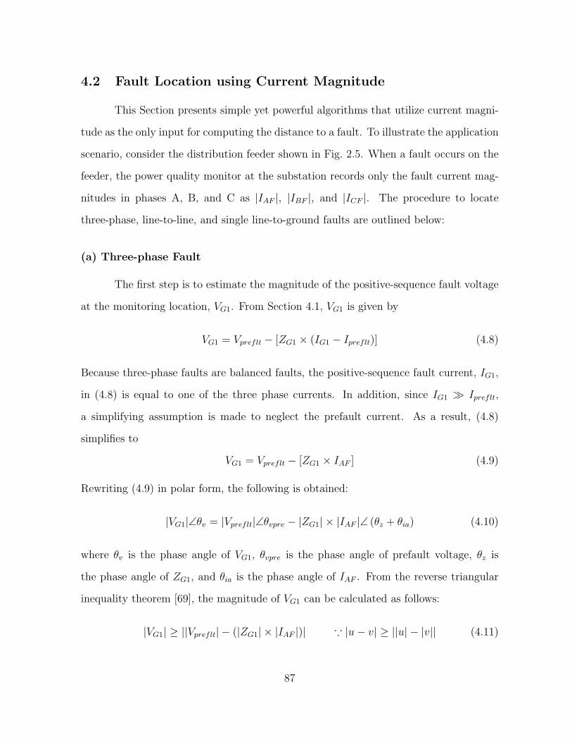
4.2 Fault Location using Current Magnitude

This Section presents simple yet powerful algorithms that utilize current magni-

tude as the only input for computing the distance to a fault. To illustrate the application

scenario, consider the distribution feeder shown in Fig. 2.5. When a fault occurs on the

feeder, the power quality monitor at the substation records only the fault current mag-

nitudes in phases A, B, and C as |IAF |, |IBF |, and |ICF |. The procedure to locate

three-phase, line-to-line, and single line-to-ground faults are outlined below:

(a) Three-phase Fault

The first step is to estimate the magnitude of the positive-sequence fault voltage

at the monitoring location, VG1. From Section 4.1, VG1 is given by

VG1 = Vpreflt − [ZG1 × (IG1 − Ipreflt)] (4.8)

Because three-phase faults are balanced faults, the positive-sequence fault current, IG1,

in (4.8) is equal to one of the three phase currents. In addition, since IG1 ≫ Ipreflt,

a simplifying assumption is made to neglect the prefault current. As a result, (4.8)

simplifies to

VG1 = Vpreflt − [ZG1 × IAF ] (4.9)

Rewriting (4.9) in polar form, the following is obtained:

|VG1|∠θv = |Vpreflt|∠θvpre − |ZG1| × |IAF |∠ (θz + θia) (4.10)

where θv is the phase angle of VG1, θvpre is the phase angle of prefault voltage, θz is

the phase angle of ZG1, and θia is the phase angle of IAF . From the reverse triangular

inequality theorem [69], the magnitude of VG1 can be calculated as follows:

|VG1| ≥ ||Vpreflt| − (|ZG1| × |IAF |)| ∵ |u− v| ≥ ||u| − |v|| (4.11)

87

The equality condition will be valid only when θvpre = θz + θia. Assuming this condition

to hold true, |VG1| can be estimated as

|VG1| = ||Vpreflt| − (|ZG1| × |IAF |)| (4.12)

Next, to estimate the fault distance, consider the positive-sequence network during a

three-phase fault as shown in Fig. 2.3. Writing the voltage drop from terminal G as

VG1 −mZL1IG1 = IFRF (4.13)

Because most faults in distribution feeders have negligible fault resistance values [14],

assume a bolted fault and express the distance to fault as

m =VG1

ZL1 × IG1

(4.14)

Rewriting (4.14) in polar form and substituting IG1= IAF

m =|VG1|

|ZL1| × |IAF |∠ (θv − θzl − θia) (4.15)

where θzl is the phase angle of the positive-sequence line impedance. Since m is a real

number, it can be calculated from only the magnitude terms as

m =|VG1|

|ZL1| × |IAF |(4.16)

It should be noted that the calculation of |VG1| in (4.12) assumes that θvpre is equal to

(θz + θia). When this condition is not fulfilled, the estimated value of |VG1| will be less

than it’s actual value. As a result, (4.16) will underestimate the location of the fault.

Put another way, the distance estimate using (4.16) can be regarded as a lower bound

for the actual fault location. However, as demonstrated in Section 4.3 and Section 4.4,

the error due to this angle mismatch is not substantial and the estimate using (4.16) is

close to the actual fault location.

88

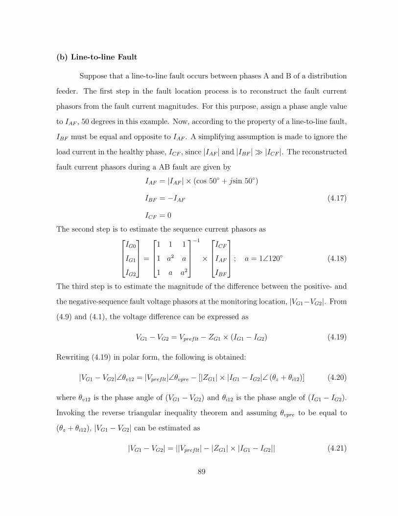
(b) Line-to-line Fault

Suppose that a line-to-line fault occurs between phases A and B of a distribution

feeder. The first step in the fault location process is to reconstruct the fault current

phasors from the fault current magnitudes. For this purpose, assign a phase angle value

to IAF , 50 degrees in this example. Now, according to the property of a line-to-line fault,

IBF must be equal and opposite to IAF . A simplifying assumption is made to ignore the

load current in the healthy phase, ICF , since |IAF | and |IBF | ≫ |ICF |. The reconstructed

fault current phasors during a AB fault are given by

IAF = |IAF | × (cos 50 + jsin 50)

IBF = −IAF

ICF = 0

(4.17)

The second step is to estimate the sequence current phasors as

IG0

IG1

IG2

=

1 1 1

1 a2 a

1 a a2

−1

×

ICF

IAF

IBF

; a = 1∠120 (4.18)

The third step is to estimate the magnitude of the difference between the positive- and

the negative-sequence fault voltage phasors at the monitoring location, |VG1−VG2|. From

(4.9) and (4.1), the voltage difference can be expressed as

VG1 − VG2 = Vpreflt − ZG1 × (IG1 − IG2) (4.19)

Rewriting (4.19) in polar form, the following is obtained:

|VG1 − VG2|∠θv12 = |Vpreflt|∠θvpre − [|ZG1| × |IG1 − IG2|∠ (θz + θi12)] (4.20)

where θv12 is the phase angle of (VG1 − VG2) and θi12 is the phase angle of (IG1 − IG2).

Invoking the reverse triangular inequality theorem and assuming θvpre to be equal to

(θz + θi12), |VG1 − VG2| can be estimated as

|VG1 − VG2| = ||Vpreflt| − |ZG1| × |IG1 − IG2|| (4.21)

89

The final step is to estimate the distance to a line-to-line fault. For this purpose, recall

that the positive- and negative-sequence fault voltages at the fault point during a line-

to-line fault are related as

VF1 − VF2 = IFRF (4.22)

Substituting the expressions of VF1 and VF2 and assuming a zero fault resistance, the

expression for fault distance can be written as

m =VG1 − VG2

ZL1 × (IG1 − IG2)(4.23)

Writing (4.23) in polar form,

m =|VG1 − VG2|

|ZL1| × |IG1 − IG2|∠ (θv12 − θzl − θi12) (4.24)

Since m is a real number, it can be estimated from only the magnitude terms as

m =|VG1 − VG2|

|ZL1| × |IG1 − IG2|(4.25)

Note that the calculation of |VG1−VG2| in (4.21) assumes θvpre to be equal to (θz + θi12).

When this condition is not fulfilled, the estimated value of |VG1−VG2| will be less than it’s

actual value. As a result, the distance estimate using (4.25) will underestimate the fault

location and can be regarded as a lower bound for the actual fault location. However,

as demonstrated in Section 4.3 and Section 4.4, the error due to this angle mismatch is

not significant and (4.25) can accurately track down the location of a line-to-line fault.

(c) Single Line-to-ground Fault

Suppose that a single line-to-ground fault occurs on phase A of a distribution

feeder. The first step in the fault location process is to estimate the sequence current

phasors at the monitoring location. Because |IBF | and |ICF | ≪ |IAF |, a simplifying

assumption is made to ignore the load currents in the unfaulted phases. As a result, the

90

sequence current calculation simplifies down to

IG0

IG1

IG2

=

1 1 1

1 a2 a

1 a a2

−1

×

IAF

0

0

; a = 1∠120 (4.26)

The magnitude of the sequence current phasors are

|IG0| = |IG1| = |IG2| =|IAF |3

(4.27)

The next step is to estimate the fault location. For this purpose, the loop impedance to

the fault, Zn, is calculated from the “pure fault” network in Fig. 4.3 as

Zn =VF,pre

IG0

− (2ZG1 + ZG0) (4.28)

Writing (4.28) in polar form, the following is obtained:

|Zn|∠θzn =|VF,pre||IG0|

∠ (θvf − θig0)− |2ZG1 + ZG0|∠θzg (4.29)

where θzn is the phase angle of the loop impedance, θvf is the phase angle of the prefault

voltage, θig0 is the phase angle of IG0, and θzg is the phase angle of (2ZG1 + ZG0).

Calculate |Zn| by applying the reverse triangular inequality theorem as

|Zn| =∣

∣

∣

∣

|VF,pre||IG0|

− |2ZG1 + ZG0|∣

∣

∣

∣

∵ ∠ (θvf − θig0) = ∠θzg (4.30)

Alternatively, the loop impedance can be calculated as

Zn = (2m× ZL1) + (m× ZL0) = m(rs + jxs) (4.31)

where rs and xs are the loop resistance and reactance in Ω/mile. The magnitude of Zn

can be calculated from (4.31) as

|Zn| = m√

(r2s + x2s) (4.32)

Equating (4.30) and (4.32), the distance to the fault can be solved as

m =

∣

∣

∣

∣

|VF,pre||IG0|

− |2ZG1 + ZG0|∣

∣

∣

∣

√

(r2s + x2s)

(4.33)

91

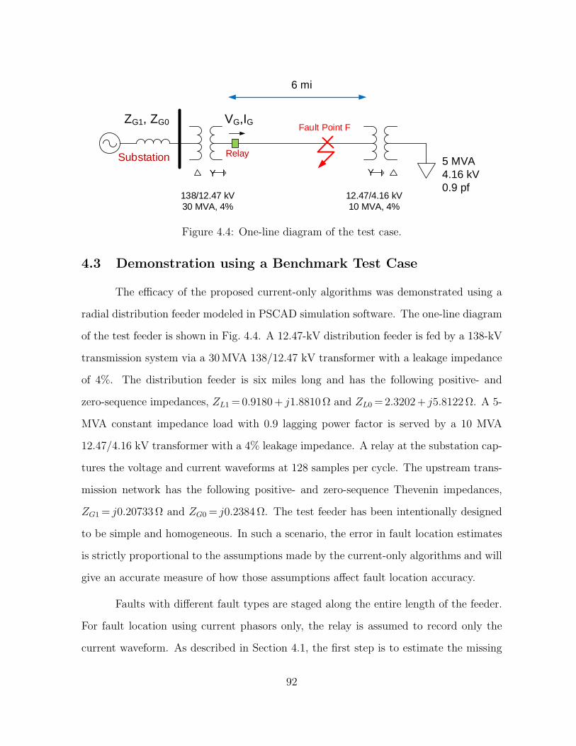
Substation

Fault Point F

5 MVA 4.16 kV0.9 pf

ZG1, ZG0 VG,IG

6 mi

12.47/4.16 kV10 MVA, 4%

138/12.47 kV30 MVA, 4%

YY

Relay

Figure 4.4: One-line diagram of the test case.

4.3 Demonstration using a Benchmark Test Case

The efficacy of the proposed current-only algorithms was demonstrated using a

radial distribution feeder modeled in PSCAD simulation software. The one-line diagram

of the test feeder is shown in Fig. 4.4. A 12.47-kV distribution feeder is fed by a 138-kV

transmission system via a 30MVA 138/12.47 kV transformer with a leakage impedance

of 4%. The distribution feeder is six miles long and has the following positive- and

zero-sequence impedances, ZL1=0.9180+ j1.8810Ω and ZL0=2.3202+ j5.8122Ω. A 5-

MVA constant impedance load with 0.9 lagging power factor is served by a 10 MVA

12.47/4.16 kV transformer with a 4% leakage impedance. A relay at the substation cap-

tures the voltage and current waveforms at 128 samples per cycle. The upstream trans-

mission network has the following positive- and zero-sequence Thevenin impedances,

ZG1= j0.20733Ω and ZG0= j0.2384Ω. The test feeder has been intentionally designed

to be simple and homogeneous. In such a scenario, the error in fault location estimates

is strictly proportional to the assumptions made by the current-only algorithms and will

give an accurate measure of how those assumptions affect fault location accuracy.

Faults with different fault types are staged along the entire length of the feeder.

For fault location using current phasors only, the relay is assumed to record only the

current waveform. As described in Section 4.1, the first step is to estimate the missing

92

fault voltage at the monitoring location. The estimated fault voltages are an exact

match with the actual fault voltages recorded by the relay as shown in Table 4.1. The

estimated fault voltages are then used by the Takagi method to successfully estimate

the fault locations.

Table 4.1: Actual vs. Estimated Fault Location using the Current Phasor Approach

Fault TypeActual Location

(mi)

Faulted Phase Voltage (kV) Estimated Location

(mi)Actual Estimated

ABC 2.00 5.47 5.47 2.00

BC 3.00 6.53 6.53 3.00

AB-G 4.00 6.44 6.44 4.00

A-G 1.50 7.04 7.04 1.50

For fault location with current magnitude only, assume that the relay records only

the current magnitude of the faulted phase. For locating the ABC fault, the approach

starts by estimating |VG1|. As seen from Table 4.2, the estimated |VG1| is lower than

it’s actual magnitude. The error can be attributed to the phase angle mismatch when

applying the reverse triangular inequality theorem to (4.12). This error, however, is

not substantial since the distance estimate using (4.16) has a fault location error of

only 0.05 miles. The location of the BC fault proceeds by estimating |VG1 − VG2|. As

seen from the table, the phase angle mismatch when applying the reverse triangular

inequality theorem to (4.21) results in |VG1 − VG2| having a lower magnitude than it’s

actual magnitude. This error is not observed to have a significant impact on fault

location accuracy since the distance estimate using (4.25) is close to the actual fault

location. The current magnitude approach cannot be applied to locate double line-to-

ground faults. For the next case of locating a single line-to-ground fault, the current

93

magnitude algorithm does not directly estimate the fault voltage. Instead, the distance

to fault is estimated from the loop impedance to fault. As seen from the table, the

estimated fault location underestimates the actual fault location due to the phase angle

mismatch when applying the reverse triangular inequality theorem in (4.30). The fault

location error is not substantial, around 0.13 miles.

Table 4.2: Actual vs. Estimated Fault Location using the Current Magnitude Approach

Fault TypeActual Location

(mi)

Faulted Phase Voltage (kV) Estimated Location

(mi)Actual Estimated

ABC 2.00 5.47 5.33 1.95

BC 3.00 5.96 5.84 2.94

AB-G 4.00 Cannot be applied

A-G 1.50 – – 1.37

Overall, the Section demonstrates the success of current-only algorithms in track-

ing down the exact location of a fault. Because of more data availability, the algorithm

using current phasors makes no assumptions when estimating the distance to a fault and

hence, has a superior performance. The algorithm using current magnitude, on the other

hand, estimates the fault location with limited data. Although several assumptions are

necessary to obtain a location estimate, the method is powerful and accurate.

4.4 Application to Field Data

This Section demonstrates the application of current-only fault locating algo-

rithms on ten fault events collected from utility distribution networks. Fault location on

two of the events is explained in details followed by a summary of the remaining events.

94

4.4.1 Event 1: Recloser Failure on a 34.5-kV Distribution Feeder

On 2 August 2010, a 34.5-kV distribution feeder experienced a single line-to-

ground fault on phase C at 3:09 pm. The fault occurred on a feeder recloser at a distance

of 3.07 miles from the substation as shown in Fig. 4.5. The distribution feeder is 5.79

miles long and is constructed using five different line configurations. The line configura-

tion used to construct the majority of the feeder length has a positive- and zero-sequence

line impedances of zL1=0.1308+ j0.5546Ω/mile and zL0=0.4029+ j1.8619Ω/mile, re-

spectively. These sequence impedances are utilized for fault location purposes. The

positive- and zero-sequence Thevenin impedances of the upstream transmission network

are ZG1=0.1480+ j3.0820Ω and ZG0=0.0028+ j0.0610Ω, respectively. Figure 4.6 il-

lustrates the voltage and current waveforms captured by a SEL-651R relay during the

fault at 32 samples per cycle. From the waveforms, it is evident that the voltage trans-

former has malfunctioned, and that the voltage data cannot be used for fault location

purposes. As a result, this event is the perfect example that demonstrates the need for

developing current-only fault location algorithms.

(a) Fault Location using Current Phasors

This event is a short-duration fault that lasts for only two cycles. As a result,

the Fast Fourier transform is applied to the second cycle after fault inception to extract

the phase C fault current phasor as 3.15∠-170 kA. The prefault current phasor is 129∠-

110A. Towards determining the fault location using current phasors only, the first step

is to estimate the prefault voltage at the monitoring location. For this purpose, the

magnitude of the prefault voltage is assumed to be 1 per unit. A load flow analysis

in the circuit model indicates that the distribution feeder is operating at 0.998 lagging

power factor. Since the prefault current has a phase angle of -110 degrees, the prefault

voltage is calculated to have a phase angle of -106 degrees. Next, using (4.3) to (4.6), the

95

Figure 4.5: Event 1 is a C-G fault on a feeder recloser at 3.07 miles from the substation.

Figure 4.6: Voltage and current waveforms recorded by the SEL-651R relay.

96

Figure 4.7: Relay at the substation records only the fault current magnitude.

fault voltage at the monitoring location, VCF,estimated, is estimated to be 12.89∠-124 kV.

This estimated voltage is then used by the Takagi method to compute the distance to

the fault to be 3.07 miles. The estimate matches exactly with the actual fault location

with no loss in accuracy.

(b) Fault Location using Current Magnitude

This approach assumes that only the current magnitude of the faulted phase,

3220A, is available for fault location purposes as shown in Fig. 4.7. Ignoring the currents

in the unfaulted phases, the sequence fault currents are determined by (4.27) as

|IG0| = |IG1| = |IG2| =|ICF |3

=3220

3= 1073.3 A

The actual sequence fault currents are:

|IG0,actual| = 1012.3 A

|IG1,actual| = 1109.8 A

|IG2,actual| = 1025.6 A

Although the healthy phase currents were ignored in the sequence fault current calcu-

lation, the estimated sequence currents are observed to be close to the actual sequence

97

currents. Next, assuming a prefault voltage magnitude of 1 per unit, the distance to

fault is computed using (4.33) to be 3.32 miles from the substation. The actual fault

location is 3.07 miles.

4.4.2 Event 2: Tree Contact Fault with a 8.32-kV Distribution Feeder

This event is a line-to-line fault that occurred between phase A and phase B of

a 8.32-kV distribution feeder on 27 June 2010 at 02:37 am. The fault was caused by a

tree falling on the overhead feeder at a distance of 0.96 miles from the substation. The

feeder has a positive- and zero-sequence line impedance of zL1=0.8817+ j1.2135Ω/mile

and zL0=1.9945+ j2.9569Ω/mile, respectively. A SEL-351A relay at the substation,

present as a backup relay, records the voltage and current waveforms during the fault

at 4 samples per cycle as shown in Fig. 4.8. However, for the purpose of evaluating the

efficacy of the current-only fault location algorithms, pretend that the voltage waveforms

are missing or not available.

(a) Fault Location using Current Phasors

From the fault current waveform recorded by the relay, the Fast Fourier transform

calculates the fault current phasors in phases B and C to be 2.86∠64 kA and 2.73∠-

112 kA, respectively. The prefault current phasor in phase A is 157∠-167A. Since the

circuit model of the distribution feeder is not available, (8.44) is used to estimate the

positive-sequence source impedance as ZG1=0.1091+ j0.8633 Ω. From the phase angles

of the voltage and current waveforms, the distribution feeder was found to operate with a

0.87 lagging power factor. It is also necessary to determine the prefault voltage phasor,

Vpreflt, for calculating the distance to fault using current phasors. The magnitude of

Vpreflt is assumed to be 1 per unit while the phase angle is calculated to be -137 using

(4.4). Next, using using (4.3) to (4.6), the fault voltages at the monitoring location are

98

Figure 4.8: Voltage and current waveforms recorded by the SEL-351A relay at thesubstation. Pretend that the voltage waveforms are missing.

estimated as follows:

VBF,estimated = 3.51∠75 kV

VCF,estimated = 2.64∠− 3 kV

The actual fault voltages are as follows:

VBF,actual = 3.40∠78 kV

VCF,actual = 2.67∠1 kV

The estimated fault voltages are observed to be close to the actual fault voltage phasors

recorded by the relay in phases B and C. Next, the estimated voltages are used by the

Takagi method to compute the distance to the fault to be 1.09 miles. The actual location

is 0.95 miles.

99

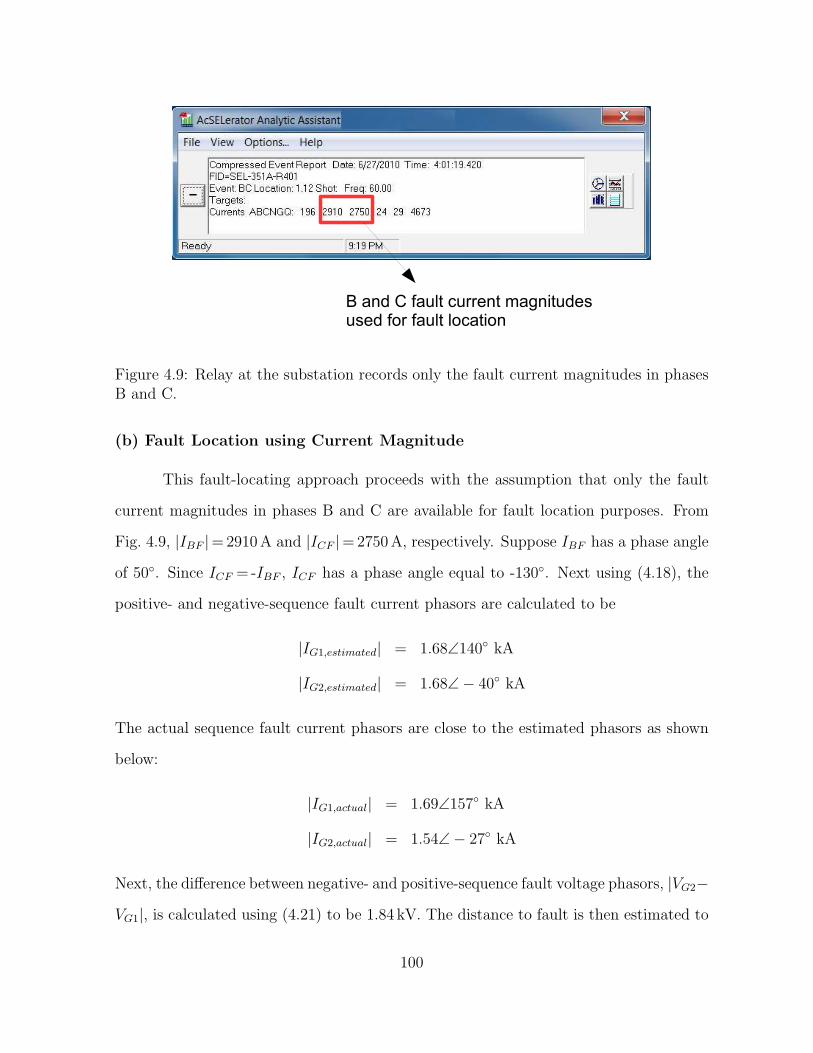
Figure 4.9: Relay at the substation records only the fault current magnitudes in phasesB and C.

(b) Fault Location using Current Magnitude

This fault-locating approach proceeds with the assumption that only the fault

current magnitudes in phases B and C are available for fault location purposes. From

Fig. 4.9, |IBF |=2910A and |ICF |=2750A, respectively. Suppose IBF has a phase angle

of 50. Since ICF = -IBF , ICF has a phase angle equal to -130. Next using (4.18), the

positive- and negative-sequence fault current phasors are calculated to be

|IG1,estimated| = 1.68∠140 kA

|IG2,estimated| = 1.68∠− 40 kA

The actual sequence fault current phasors are close to the estimated phasors as shown

below:

|IG1,actual| = 1.69∠157 kA

|IG2,actual| = 1.54∠− 27 kA

Next, the difference between negative- and positive-sequence fault voltage phasors, |VG2−

VG1|, is calculated using (4.21) to be 1.84 kV. The distance to fault is then estimated to

100

be 0.88 miles. The actual location is 0.95 miles.

4.4.3 Fault Location Analysis of the Remaining Events

Fault location analysis on all the remaining events are summarized in Table 4.3.

Event 3 is a single fault at 1.42 miles from the substation. The sub-events correspond

to the fast and slow operation of a downstream recloser. In certain sub-events, the

fault location using current phasor approach cannot be applied due to the absence of

prefault data. In Event 6, the fault evolves from a line-to-line to a three-phase fault and

back to a line-to-line fault in a matter of few seconds. In Event 8, the utility reports

a possible fault location of 2.50 miles. However, as per the analysis conducted using

existing impedance-based fault location algorithms, the fault is suspected to be located

at 0.33 miles from the substation. Estimates from the current-only algorithms support

this conclusion as well. The analysis in Event 9 reveals that the distribution feeder had,

in fact, experienced two faults: a A-G fault that evolved into a ABC fault at 4.27 miles,

and another AB fault at 0.55 miles. This reasoning is further supported by the dramatic

increase in fault current from 3.4 kA to 6.8 kA in Event 9g.

Overall, the analysis of field data proves that the proposed current-only algo-

rithms are successful in tracking down the exact location of a fault with no significant

loss in accuracy. For this dataset, the fault location approach using only the current

phasor is accurate within 0.37 miles while the fault location approach using only the

current magnitude is accurate within 0.81 miles of the actual fault location.

101

Table 4.3: Actual vs. Estimated Location using Current Phasors and Current Magnitude

Event Fault TypeActual Location

(mi)

Estimated Fault Location (mi)

Voltage and Current

Phasors

Current

Phasor

Current

Magnitude

3a AB 1.42 1.49 1.30 1.35

3b AB 1.42 1.47 1.53 1.43

3c AB 1.42 1.47 Prefault data

absent

1.41

3d AB 1.42 1.45 1.14 1.40

3e AB 1.42 1.44 Prefault data

absent

1.32

4a BG 1.70 1.62 1.81 1.93

4b BG 1.70 1.68 Prefault data

absent

2.39

5 AG 10.70 10.72 10.68 11.41

6a AB 1.51 1.70 1.65 1.59

6b AB 1.51 1.68 Prefault data

absent

1.59

6c AB 1.51 1.65 1.57

6d ABC 1.51 1.54 ...1.72

6e ABC 1.51 1.47 ...1.78

6f AB 1.51 1.69 ...1.61

6g AB 1.51 1.71 1.72

7 CG 5.33 4.82 4.96 4.52

8 BG 2.50 0.33 0.32 0.36

9a AG 4.27 4.24 4.27 4.14

9b ABC 4.27 3.97 3.94 3.76

9c ABC 4.27 4.00 Prefault data

absent

3.87

9d ABC 4.27 3.96 4.18 3.66

9e ABC 4.27 4.03 Prefault data

absent

3.89

9f AB 4.27 0.55 0.44 0.23

9g AB 4.27 0.58 Prefault data

absent

0.49

9h AB 4.27 0.16 0.03

9i ABC 4.27 3.98 4.14 3.64

9j ABC 4.27 4.01 Prefault data

absent

3.91

10a AG 0.28 0.24 0.24 0.28

10b BC 0.28 0.20 Prefault data

absent

0.14

102

4.5 Short-circuit Fault Current Profile Method

The short-circuit fault current profile method uses the circuit model of the distri-

bution feeder to determine the location of a fault. The approach is to simulate the same

fault in the circuit model along the entire length of the feeder. The location at which

the short-circuit current matches with the measures fault current magnitude is selected

as the actual fault location. The method does not require voltage measurements and

has a high level of accuracy as demonstrated in [57,70].

4.6 Summary

This Chapter proposes practical fault location algorithms that use only the cur-

rent data recorded by a relay to estimate the distance to a fault. Two fault locat-

ing approaches using current phasors and current magnitude are developed. Both ap-

proaches work by estimating fault voltage at the monitoring location and then invoking

impedance-based fault-locating principles. Analysis on simulation and field data showed

promise. The fault location approach using only the current phasors is accurate within

0.31 miles while the fault location approach using only the current magnitude is accu-

rate within 0.71 miles of the actual fault location. The Chapter also presents another

approach that uses the fault current phasor or fault current magnitude and the system

circuit model for fault location purposes.

103

Chapter 5

Effects of Distributed Generators on Fault Location

One-ended impedance-based fault location algorithms such as the simple reac-

tance, Takagi, and Novosel et al. methods are commonly used to locate faults in dis-

tribution networks. These algorithms assume a radial distribution feeder with a unidi-

rectional flow of power from the substation to the end users as discussed in Chapter 2.

With the integration of distributed generators to the distribution circuit, however, dis-

tribution feeders are no longer radial. Short-circuit current to a fault comes from two

sources, the utility substation and distributed generators. Since the level of penetration

of DGs is expected to increase over the next few years, ignoring the latter term will

certainly compromise the accuracy of location estimates.


evaluate the effect of distributed generators on the accuracy of existing impedance-

based fault-locating algorithms. The focus is on faults that occur downstream from

DGs. This is because when faults are located upstream from distributed generators,

fault current contributed by DGs act as a source of remote infeed and will not have a

significant impact on fault location accuracy [71]. Authors in [72] investigate the im-

pact of DG technology on impedance-based fault location algorithms. They conclude

that synchronous generators have the worst impact on fault location algorithms since

the short-circuit current from these generators is five to ten times the rated current.

Authors in [30] conduct simulation studies to demonstrate the impact of other factors

such as MVA capacity of the DG unit, tapped loads, and location of the fault from DG

104

on fault location estimates. Simulation studies are, however, not helpful in understand-

ing how these factors act as a source of error. The contribution of this Chapter is

that it provides a detailed insight into how each of the factors mentioned above affect

impedance-based fault location algorithms in the presence of DGs and how to interpret

the results. A detailed understanding of error sources is useful for developing improved

fault locating solutions. Furthermore, this Chapter investigates additional factors that

may influence fault location downstream from DGs. They are fault resistance and con-

figuration of the DG interconnect transformer.

The analysis in this Chapter concludes that higher the MVA capacity of the DG

unit, greater is the error in fault location. If faults occur very close to DGs, the error in

fault location is marginal. As the fault moves further downstream from DGs, the error

increases significantly. Although tapped loads counter the effect of DGs, the improve-

ment in fault location accuracy is not significant. Reactance error due to fault resistance

can cancel out the effect of DGs or further magnify the error in location estimates. Un-

der such circumstances, an improved fault locating algorithm proposed in Chapter 6 is

recommended. Only if DG interconnect transformers have a delta configuration on the

utility side, DGs will not contribute any current during a single line-to-ground fault. In

such cases, existing impedance-based fault locating methods may still be used.

The Chapter is organized as follows: Section 5.1 presents a discussion on how dis-

tributed generators act as a source of short-circuit current and compromise the accuracy

of locating faults that occur downstream from DGs, Section 5.2 develops a time-domain

model of a distribution feeder, Section 5.3 uses this model to evaluate the critical factors

that affect impedance-based fault locating algorithms when DGs are interconnected to

the distribution feeder, and Section 5.4 summarizes the key findings of the Chapter.

105

Publications:

– S. Das, S. Santoso, and A. Maitra, “Effects of distributed generators on

impedance-based fault location algorithms,” in Proc. IEEE PES General

Meeting Conf. Expo., Jul. 2014, pp. 1-5.

5.1 Impact of DGs on Impedance-based Fault Location

As seen in Chapter 2, impedance-based fault location algorithms assume a ra-

dial distribution feeder where power flows unidirectionally from the substation to the

end users. However, with increased penetration of distributed generators (DGs) to the

distribution circuit, distribution feeders are no longer radial. When a fault occurs down-

stream from the DG unit, DGs contribute to the total fault current and will modify

the apparent impedance seen from the substation. To illustrate this concept, consider

the distribution feeder shown in Fig. 5.1. The feeder has a total positive-sequence line

impedance of ZL1 ohms. The DG is interconnected to the feeder (referred to as the

point of interconnection or POI) at a distance d per unit from the substation. When a

three-phase fault with a fault resistance RF occurs at a distance of m per unit from the

substation, the substation and DG operate in parallel to feed the fault.

dZL1

IGSubstation

IDGVG

F(m-d)ZL1

DG

Load

(1-m)ZL1

IG+IDG

d

m

RF

POIIF

Zapp

Figure 5.1: Distribution feeder with a fault located downstream from the DG.

106

Voltage drop from the substation can be written as,

VG = dZL1IG + (m− d)ZL1 (IG + IDG) +RF IF (5.1)

where VG and IG are the voltage and current phasors recorded at the substation during

the fault, IDG is the fault current from the DG unit, and IF is the current at the fault

point. Dividing throughout by IG and simplifying, the apparent impedance (Zapp) seen

from the substation is

Zapp =VG

IG= mZL1 + (m− d)ZL1

IDG

IG+RF

(

IFIG

)

(5.2)

As evident from (5.2), when the fault is located downstream from the DG unit, the

apparent impedance seen from the substation is proportional to the impedance to the

fault (mZL1) as well as two additional terms: (m − d)ZL1 (IDG/IG) and RF (IF/IG).

Since one-ended fault locating methods make use of only VG and IG at the substation,

neglecting IDG in (5.2) will certainly compromise the accuracy of the location estimates.

For a bolted fault, the term (m − d)ZL1 (IDG/IG) increases Zapp as shown in

Fig. 5.2 (a). As a result, impedance-based fault location algorithms will overestimate

the location of the fault. When the fault has a significant RF , impedance-based fault

location algorithms are affected by an additional reactance error. Since short-circuit

current at the fault point (IF ) comes from the utility substation (IG) and the distributed

generator (IDG), phase angles of IF and IG are not equal to each other. When IF leads

IG, the term RF (IF/IG) is inductive, and together with (m− d)ZL1 (IDG/IG) increases

the apparent impedance to the fault as shown in Fig. 5.2 (b). This is the worst case

scenario and fault location algorithms will significantly overestimate the fault location.

When IF lags IG, on the other hand, RF (IF/IG) is capacitive and will attempt to cancel

out the effect of (m− d)ZL1 (IDG/IG) as illustrated in Fig. 5.2 (c).

In summary, when a fault occurs downstream from DGs, fault location error

from the one-ended algorithms will depend on the magnitude of (m − d)ZL1 (IDG/IG)

107

mZ L1

R

jX

0

F

(a) RF = 0 Ω (b) RF ≠ 0 Ω, IF leads IG

mZ L1

R

jX

0

F

mZ L1

R

jX

0

F

(c) RF ≠ 0 Ω, IF lags IG

Z app Z ap

p

Z app

(m-d

)Z L1I DG

IG

(m-d

)ZL1I DG

IG

(m-d

)ZL1

I DG

IG

IF

IGRF

IF IG

RF

Figure 5.2: Apparent impedance Zapp from the substation

and RF (IF/IG). Several factors can affect the magnitude of these terms and hence, the

accuracy of location estimates. These factors are investigated in Section 5.3.

5.2 Distribution Test Case Feeder

This Section describes a distribution feeder which will serve as a test bed for

evaluating the different factors that affect fault location downstream from DGs. The

test feeder was modeled in PSCAD simulation software [47] and is capable of replicating

actual faults occurring in a distribution feeder. Fig. 5.3 shows the single line diagram

of the test feeder. The transmission network upstream from the distribution feeder is

represented by an ideal voltage series behind an equivalent positive- and zero-sequence

Thevenin impedance of Zeq1 = j3.81 Ω and Zeq

0 = j11.43 Ω, respectively. A 10-MVA,

delta/wye-grounded transformer with a leakage impedance of 4% is used to step down

the voltage from 138 to 13.8 kV. A power quality monitor at the substation records the

three-phase line-to-ground voltages and line currents at 128 samples per cycle. The main

distribution feeder is 6 miles long and has a line configuration shown in Fig. 5.4. The

108

Transmission System

2 mi 4 mi

Constant Impedance Load12 MVA, 13.8 kV, 0.9 pf

IG

VG

POId

138/13.8 kV10 MVA, 4%

Y

XD

G

Unit 1

XD

G

XD

G

Y

6.9/13.8 kV8 M

VA

, 4% 2 mi

Individual DG Unit:Synchronous Generator2 MVA, 6.9 kV

Unit 2 Unit 3

XDG,1 = j1.29 Ω

XDG,0 = j0.60 Ω

Z1eq = j3.81 Ω

Z0eq = j11.43 Ω

Monitoring Location

Figure 5.3: One-line diagram of the distribution test case feeder.

phase and neutral conductors are built using an all-aluminum conductor (AAC) of size

336 AWG. Using Carson’s equations [3], the positive- and zero-sequence line impedances

were calculated to be ZL1,1 = 0.2780 + j0.6584 Ω/mi and ZL1,0 = 0.5474 + j1.9720 Ω/mi,

respectively. These line impedances will be used for fault location in Section 5.3.

The distribution feeder serves a 12-MVA constant impedance load with a 0.9

lagging power factor. Part of this load is supported by the substation, limited only by the

size of the 10-MVA transformer. The remaining load is served by three diesel generator

units that are interconnected to the POI via a 2-mile long feeder. Each unit, rated at 2

MVA, consists of a diesel engine acting as a prime mover to a synchronous generator. In

this analysis, synchronous generators were chosen since fault current contributed by these

generators have the worst impact on fault location algorithms [72]. The generator was

modeled as a voltage source behind a sub-transient reactance, Xd”. This simple model

is sufficient for performing short-circuit studies [2]. Machine constants of a Caterpillar

diesel generator were used [2] and are listed in Table 5.1. Notations XDG,2 and XDG,0

109

A

26'

34'

3.7' 3.7'

B

C

N

1'

Figure 5.4: Line geometry of the 13.8-kV overhead distribution feeder.

refer to the negative- and zero-sequence generator reactance while the positive-sequence

reactance of the generator (XDG,1) is equal to Xd”. An 8-MVA, delta/wye-grounded

transformer with a leakage impedance of 4% interfaces the DG units to the feeder. The

DG units appear to be “effectively grounded” since [33]

R0

X1

= 0 < 1 andX0

X1

= 0.36 < 3

where R0 is the zero-sequence resistance, X0 and X1 are the zero- and positive-sequence

reactances, respectively at the high voltage side of the DG interconnect transformer.

Note that the test feeder has been intentionally designed to be simple, homoge-

neous, and compliant with the other assumptions [13] made by impedance-based fault

locating algorithms. In such a scenario, the error in fault location estimates will be

strictly proportional to the fault current contributed by DGs and will give an accurate

measure of how DGs affect fault location accuracy.

110

Table 5.1: CAT SR4-HV Synchronous Generator Data [2]

Parameter Data

Gen Manufacturer Cat SR4-HV

Type of DG Diesel

MVA-Continuous 2

Voltage (kV) 6.9

Xd” (pu) 0.162

XDG,0 (pu) 0.0752

XDG,2 (pu) 0.162

5.3 Factors that Affect Fault Location Downstream from DGs

5.3.1 DG Technology

The magnitude and duration of the fault current contributed by distributed gen-

erators (IDG) depends on the electrical converter that DGs use to interconnect to the

distribution feeder. According to the IEEE Standard 1547 [73], there are three types

of electrical converters: synchronous machines, induction machines, and inverter-based

DGs. Synchronous machines used by diesel generators, gas turbines and hydro genera-

tors provide a sustained fault current and have the worst impact on impedance-based

fault locating algorithms [71]. Fault current is 5 to 10 times the rated current during the

sub-transient period and then decays to 2 to 4 times the rated current [33]. Induction

generators, used in fixed-speed and wide-slip wind turbines, can also contribute to a

fault so long as the residual voltage on the healthy phase can establish a rotating mag-

netic field. Although the initial magnitude of the fault current is 5 to 10 times the rated

current, the current decays at a rate which depends on the fault type [34]. As a result,

the error in fault location depends on the fault type and also on the cycle chosen for

fault location. Inverter-based DGs such as fuel cells, photovoltaic generators, double-fed

induction generator (DFIG), and permanent magnet wind turbines contribute fault cur-

rent for less than half a cycle [33]. In the worst case, if inverter-based DGs continue to

111

feed a fault, the fault current is only 1 to 2 times the rated current. The corresponding

error in fault location estimates is, therefore, lower than other DG technologies [71].

5.3.2 DG Interconnect Transformer

Configuration of the step-up transformer that interfaces the distributed generator

to the distribution feeder is an important consideration when applying impedance-based

fault location algorithms. If the transformer is connected as a delta on the utility side,

then DGs will not contribute any zero-sequence current during a single line-to-ground

fault. As a result, the fault location error will be lower than when the transformer is

wye-connected. Recall that single line-to-ground faults are the most common amongst

all other types of fault.

5.3.3 Size of the DG Unit

The magnitude of IDG in terms (m − d)ZL1 (IDG/IG) and RF (IF/IG) of (5.2)

depends on the MVA capacity of the installed distributed generators. Single DG units

with a small MVA capacity do not contribute a significant fault current. However, when

the MVA capacity is increased by aggregating a number of small or a few large DG units,

the equivalent generator impedance decreases [33]. As a result, the total fault current

from DGs increase and can significantly offset the accuracy of fault location algorithms.

To demonstrate how the MVA capacity of the DG unit affects fault locating algo-

rithms, consider the test feeder developed in Section 5.2. At a particular instant of time,

suppose that only Unit 1 DG is in operation while the remaining generators are switched

off. When a single line-to-ground fault on phase A (RF = 0 Ω) occurs at a distance of 4

miles from the substation, Unit 1 DG contributes a fault current of 0.47 kA. Using VG

and IG recorded at the substation, location estimates from the impedance-based meth-

ods are shown in Table 5.2. Now, when Unit 2 DG is brought online along with Unit

112

1, then for the same fault, the total fault current at the DG terminal (IDG) is 0.62 kA.

This is because both the generators are in parallel and the equivalent impedance reduces

to 0.08 pu. Since IDG increases, the error in fault location also increases. Similarly, if a

fault occurs when all the three DG units are in operation, the magnitude of IDG is even

higher, and the error in fault location increases proportionally.

Table 5.2: Impact of DG MVA Size on Fault Location Algorithms

DG Size Xd” IDG ActualEstimated Location (mi)

(MVA) (pu) (kA) Location (mi) Simple Reactance Takagi Novosel et al.

2 0.16 0.474

4.84 4.86 4.844 0.08 0.62 5.01 5.04 5.016 0.05 0.73 5.14 5.17 5.14

5.3.4 Fault Distance from the DG Unit

As discussed in Section 5.1, when a bolted fault occurs downstream from the DG,

the error in fault location primarily stems from the term (m−d)ZL1 (IDG/IG). Location

of the fault m affects the magnitude of this term in two ways: factors (m − d) and

the current ratio IDG/IG. When a fault occurs at the POI, the fault is very close to

the distributed generator. Current IDG and, therefore, IDG/IG is maximum. However,

because m is equal to d, the term (m − d)ZL1 (IDG/IG) becomes zero and DG will not

affect the accuracy of location estimates.

The impact of how the distance to fault from the DG unit affects impedance-based

fault location algorithm is illustrated by using the test case developed in Section 5.2. A

single line-to-ground fault (RF = 0 Ω) on phase A is simulated at a distance of 2 miles

from the substation. Since the DG is also interconnected to the feeder at 2 miles, the

term (m−d)ZL1 (IDG/IG) becomes zero and DG has no impact on impedance-based fault

113

Table 5.3: Effect of Distance of the Fault from the DG Unit on Fault Location Algorithms

Actual

Location

(mi)

m− d

(mi)

IDG

IGimag

[

(m− d)ZL1IDG

IG

]

(Ω)


Simple

ReactanceTakagi

Novosel

et al.

2 0 0.60∠− 3.7 j0.0000 2.00 2.00 2.00

3 1 0.59∠− 5.4 j0.3697 3.56 3.57 3.56

4 2 0.57∠− 7.2 j0.7096 5.08 5.10 5.08

5 3 0.56∠− 9.2 j1.0192 6.55 6.60 6.55

location algorithms as shown in Table 5.3. When the same fault is simulated further

downstream from DGs, (m−d) increases. The current ratio IDG/IG, on the other hand,

decreases since impedance to the fault increases. As seen in Table 5.3, this decrease in

the current ratio is small. The increase in (m− d) is the dominating factor. As a result,

the corresponding error in the fault location estimates increase significantly.

5.3.5 Fault Resistance

To investigate how fault resistance affects fault location algorithms in the presence

of distributed generators, a single line-to-ground fault on phase A is simulated in the

test feeder at a distance of 4 miles from the substation. The fault resistance was varied

from 0 to 10 Ω. As seen in Table 5.4, when RF = 0 Ω, the reactance error due to

imag(RF (IF/IG)) is zero. Because of the fault current contributed by DGs, the term

(m−d)ZL1 (IDG/IG) in (5.2) increases the apparent impedance seen from the substation

(Zapp). As a result, fault location algorithms overestimate the location of the fault.

When the same fault is simulated with a fault resistance of 4 Ω, the reactance error is

capacitive as seen in Table 5.4. In this case, the reactance error decreases Zapp while the

term (m − d)ZL1 (IDG/IG) tends to increase Zapp. As a result, location estimates from

the simple reactance method improve as shown in Table 5.4. For RF =8Ω, however,

the reactance error is inductive. This is the worst case scenario since both the reactance

114

Table 5.4: Impact of RF on Impedance-based Fault Locating Algorithms when the Faultis Downstream from DGs

RF

(Ω)ActualLocation(mi)

imag

[

(m− d)ZL1IDG

IG

]

(Ω)

imag

[

RF × IFIG

]

(Ω)


SimpleReactance

TakagiNovoselet al.

0 j0.7096 j0.0000 5.08 5.10 5.08

4 4 j0.6569-j0.1398

(Capacitive)5.05 5.52 4.79

8 j0.6150j0.0937

(Inductive)5.54 5.86 4.58

error and (m− d)ZL1 (IDG/IG) increase Zapp. As a result, simple reactance and Takagi

methods overestimate the location of the fault. It is interesting to observe that for non-

zero values of RF , accuracy of estimates from the Novosel et al. method improve as seen

in Table 5.4. This does not indicate a good estimate. Rather, the error due to fault

resistance is canceling out the effect of DG.

5.3.6 Tapped Load

Impedance-based fault locating algorithms assume that loads served by a distri-

bution feeder are lumped at the end of the feeder [13]. In practice, loads are tapped along

the entire length of the feeder as shown in Fig. 5.5. When a bolted fault (RF = 0 Ω)

occurs at point F as shown in Fig. 5.5, the actual impedance between the substation

and the fault point F, ZGF , is

ZGF = ZGT + ZTF (5.3)

where ZGT is the positive-sequence impedance of the line segment between the substation

and the tap point, and ZTF is the positive-sequence line impedance between the tap point

and the fault. However, due to tapped loads, relay G uses VG and IG to measure the

115

FZGT ZTF

Tap

Load

Zapp

Load

Substation

VG, IG

Figure 5.5: Loads tapped along the entire length of the distribution feeder.

apparent impedance to be

Zapp =VG

IG= ZGT +

ZTF × ZLoad

ZTF + ZLoad

< ZGF . (5.4)

Since ZLoad has a much higher impedance than ZTF , the resultant value of

(

ZTF × ZLoad

ZTF + ZLoad

)

in (5.4) is closer to but slightly smaller than ZTF [30]. In other words, tapped loads act

as a negative impedance and Zapp is smaller than the actual impedance to the fault, ZGF .

In contrast, fault current contribution from DGs (IDG) increase Zapp seen from the sub-

station. Therefore, the two error factors, tapped load and IDG, tend to cancel out each

other and can help improve the accuracy of impedance-based fault locating algorithms.

The positive effect of tapped loads in locating faults that occur downstream from

DGs is illustrated using the test feeder in Section 5.2. A single line-to-ground fault on

phase A (RF =0Ω) is simulated at a distance of 4 miles from the substation. In the first

case, the load is lumped at the end of the feeder. As expected, using VG and IG at the

substation, impedance-based algorithms overestimate the location of the fault as shown

in Table 5.5. In the second case, the 12-MVA load is tapped at the POI. The tapped

load, acting as a negative impedance, counters the effect of IDG in increasing Zapp. As

a result, fault location accuracy improves, albeit marginally.

116

Table 5.5: Impact of Load Taps on Fault Locating Algorithms

Load Tap Actual LocationEstimated Location (mi)

(mi) Simple Reactance Takagi Novosel et al.

No4

5.08 5.10 5.08

Yes 4.97 5.01 4.98

5.4 Summary

This Chapter concludes that the accuracy of impedance-based fault locating al-

gorithms are compromised when faults occur downstream from distributed generators.

The Chapter also identifies a number of factors which influence the magnitude of the

fault location error. Synchronous DGs result in a higher fault location error as compared

to inverter-based DGs while the fault location error due to induction generators depends

on the fault type. The error in fault location also depends on the installed MVA capacity

of the DG unit. Higher the MVA capacity, greater will be the error in fault location.

DG interconnect transformers with a delta configuration on the utility side prevents the

flow of zero-sequence currents during a ground fault. As a result, there will be no error

in locating single line-to-ground faults. Tapped loads may counter the negative effect of

DGs and help improve the accuracy of location estimates. Reactance error due to fault

resistance may aid or further decrease the accuracy of location estimates. Finally, if a

fault is located very close to the DG unit, the error in location estimates is negligible. As

the fault moves further downstream from the DG unit, the fault location error increases

significantly.

117

Chapter 6

An Impedance-based Fault-Locating Technique for

Distribution Networks with Distributed Generators

As discussed in Chapter 5, the accuracy of existing impedance-based fault loca-

tion algorithms deteriorate when locating faults downstream from distributed generators

(DGs) in a distribution feeder. Short-circuit current to a fault comes from two sources,

the utility substation and the distributed generators. Neglecting the latter term in the

fault location calculation severely compromises the accuracy of impedance-based algo-

rithms. Algorithms proposed by [26–28] aim to improve fault location accuracy in the

presence of DGs. Unfortunately, these algorithms require additional measurements at

the DG terminal that may not be available. Authors in [29] present an interesting, but it-

erative approach that utilize measurements captured at the substation only. Algorithms

in [30] and [31] also make use of substation measurements; however, their application is

limited to line-to-line and three-phase faults, respectively.

Based on the background mentioned above, the objective of this Chapter is to

present a methodology that improves the accuracy of locating faults downstream from

distributed generators. The contribution is based on the fact that the proposed algo-

rithm uses only the voltage and current at the substation and the distributed generator

impedance to estimate the missing fault current at the DG terminal. The estimated

current is then included in the fault location calculation to improve the fault location

accuracy. The proposed algorithm is non-iterative, straightforward to implement, and

capable of locating single line-to-ground, line-to-line, double line-to-ground, and three-

phase faults. When validated against an actual 34.5-kV distribution feeder, the distance

118

estimates from the proposed approach are within 0.5 miles of the actual fault location.

The improvement in fault location accuracy over conventional algorithms is 0.56 miles.

6.1 Overview of the Proposed Approach

Chapter 5 demonstrates that the fault location error of existing impedance-based

fault location algorithms is proportional to the magnitude of the following terms: (m−

d)ZL1 (IDG/IG) and RF (IF/IG). The approach proposed in this Chapter focuses on

addressing each of those error terms to improve the accuracy of location estimates. For

example, consider the scenario shown in Fig. 5.1. To eliminate the fault location error

due to (m − d)ZL1 (IDG/IG), the approach is to estimate the fault current contributed

by the distributed generator, IDG. Data required consists of voltage and current at the

substation and the distributed generator impedance. The generator impedance can be

obtained from manufacturer specifications, an example of which is shown in Table 5.1.

The estimated IDG is then incorporated into the fault location calculation to negate the

error due to (m − d)ZL1 (IDG/IG). The next step is to minimize the reactance error

due to RF (IF/IG). For this purpose, observe that the distribution feeder in Fig. 5.1 is

radial at the POI and that the current at the fault point, IF , has a phase angle close

to the current at the POI, IPOI . As a result, the reactance error can be minimized by

using the voltage and current measurements at the POI for fault location. This step is

equivalent to moving the monitoring location “electrically” from the substation to the

POI as illustrated in Fig. 6.1.

6.2 Step-by-Step Derivation of the Proposed Approach

This Section presents a step-by-step derivation of the proposed approach for

locating a single line-to-ground fault. The same principle can be extended for locating

line-to-line, double line-to-ground, and three-phase faults.

119

dZL1

IGSubstation

IDGVG

F(m-d)ZL1

DG

Load

(1-m)ZL1

IPOI

d

m

RF

POIIF

Move the Monitoring Location to the POI

Figure 6.1: Move the monitoring location “electrically” from the substation to the POI.

Step 1: Estimate the Fault Current Contributed by DGs

The sequence network during a single line-to-ground fault is shown in Fig. 6.2.

When a fault occurs downstream from the point of interconnection (POI), the substation

and DGs operate parallel to each other while feeding the fault. As a result, the negative-

sequence fault voltage at the POI, VPOI2, is the same when calculated from the substation

or the DG terminal as shown below:

Substation: VPOI2 = VG2 − dZL2IG2 (6.1)

DG terminal: VPOI2 = −ZDG2IDG2 (6.2)

where VG2 and IG2 are the negative-sequence fault voltage and current at the substation,

IDG2 is the negative-sequence fault current from the DG terminal, d is the distance

between the POI and the substation, ZDG2 is the equivalent negative-sequence Thevenin

impedance between the DG and POI, and ZL2 is the negative-sequence line impedances.

Equating (6.1) with (6.2), IDG2 can be estimated as

IDG2 =dZL2IG2 − VG2

ZDG2

(6.3)

120

Using the same principle, the zero-sequence fault current from the DG terminal, IDG0,

can be estimated as

IDG0 =dZL0IG0 − VG0

ZDG0

(6.4)

where VG0 and IG0 are the zero-sequence fault voltage and current at the substation,

ZDG0 is the equivalent zero-sequence Thevenin impedance between the DG and POI,

and ZL0 is the zero-sequence line impedances.

The calculation of the positive-sequence fault current from the DG terminal,

IDG1, on the other hand, is complicated by the presence of the internal source voltages.

For this purpose, the superposition theorem is used to decompose the network during

fault into a prefault and “pure fault” network as shown in Fig. 6.3. Fault current IDG1

is, therefore, the summation of the prefault and the “pure fault” current, IDGpre and

∆IDG1, respectively. The estimation of ∆IDG1 is straightforward and is given by

∆IDG1 =dZL1∆IG1 −∆VG1

ZDG1

(6.5)

where ∆VG1 = VG1 − VGpre, ∆IG1 = IG1 − IGpre, VG1 and IG1 are the positive-sequence

fault voltage and current at the substation, VGpre and IGpre are the prefault voltage

and current at the substation, and ZDG1 is the equivalent positive-sequence impedance

between the DG and POI. The prefault current, IDGpre, can be estimated as

|IDGpre| =SDG√

3× |VDGpre|(6.6)

where SDG is the rated power output of the DG unit and |VDGpre| is 1 per unit. The

phase angle of IDGpre can be obtained by assuming that IDGpre lags VPOIpre by the power

factor of the load. The calculation of VPOIpre is given by (6.7).

Step 2: Move the Monitoring Location “Electrically” to the POI

To minimize the reactance error due to fault resistance RF , the monitoring loca-

tion is moved “electrically” to the POI as illustrated in Fig. 6.1. The new set of voltage

121

EG

IF

VG1

VF1

+VPOI1

+

IDG1

IPOI1

IG1

VDG1

EDG

VG2

VF2

+VPOI2

+

IDG2

IPOI2

IG2

VDG2

VG0

VF0

+VPOI0

+

IDG0

IPOI0

IG0

VDG0

ZG0 (m-d)ZL0 (1-m)ZL0

ZDG0

dZL0

ZLoa

d,0

3RF


ZDG2

dZL2

ZLoa

d,2ZG1 (m-d)ZL1 (1-m)ZL1

ZDG1

dZL1Z

Load,1


and current measurements at the POI can be computed from the substation measure-

ments and will be used to solve for the distance to fault. For example, the prefault

voltage and current phasors at the POI, VPOIpre and IPOIpre, can be calculated as:

VPOIpre = VGpre − dZL1IGpre

IPOIpre = IGpre + IDGpre

(6.7)

122

VF,pre

3RF IF

∆VG1

∆V1F

+∆VPOI1

+

∆IDG1

∆IG1+∆IDG1

∆IG1

∆VDG1

VG2

VF2

+VPOI2

+

IDG2

IPOI2

IG2

VDG2

VG0

VF0

+VPOI0

+

IDG0

IPOI0

IG0

VDG0

EG

VGpre

VF,preVPOIpre

IDGpre

IGpre+IDGpre

IGpre

VDGpre

EDG

+

Pre

faul

tP

ure

Fau

lt


ZDG0

dZL0

ZLoa

d,0

ZG2(m-d)ZL2 (1-m)ZL2

ZDG2

dZL2 ZLo

ad,2


ZDG1

dZL1 ZLo

ad,1


ZDG1

dZL1

ZLoa

d,1

Figure 6.3: Superposition principle used to decompose the network into a prefault and“pure fault” network.

123

The positive-, negative-, and zero-sequence fault voltage phasors at the POI, VPOI1,

VPOI2, and VPOI0 are:

VPOI1 = VG1 − dZL1IG1



∴ VPOI = VPOI1 + VPOI2 + VPOI0

(6.8)

The positive-, negative-, and zero-sequence fault current phasors at the POI, IPOI1,

IPOI2, and IPOI0 are:

IPOI1 = IG1 + IDG1

IPOI2 = IG2 + IDG2

IPOI0 = IG0 + IDG0

∴ IPOI = IPOI1 + IPOI2 + IPOI0

(6.9)

Step 3: Apply Impedance-based Methods from the POI

The voltage and current phasors at the POI can be used in existing impedance-

based fault location algorithms to estimate the distance to the fault. As an example,

the simple reactance method computes the distance to fault as

m =

imag

(

VPOI

IPOI + kIPOI0

)

imag [(1− d)× ZL1]+ d (6.10)

124

6.3 Description of the Test Distribution Feeder

An actual 34.5-kV distribution feeder serving utility customers in rural New York

was used to demonstrate the efficacy of the proposed approach. Customers on this feeder

experience power outages longer than 10 hours. The high restoration time can be at-

tributed to the fact that the distribution feeder is fed by a single radial transmission or

sub-transmission supply line. Furthermore, maintenance crew need time to travel to the

remote area and patrol the entire line length to find the fault location. Therefore, to

reduce downtime and achieve the state Customer Average Interruption Duration Index

(CAIDI) target of 2.5 hours, one part of the proposed solution was to develop a micro-

grid. For this purpose, a 416-kW biomass diesel generator and a 6.6-MW wind farm were

interconnected to the distribution feeder as shown in Fig. 6.4. Under normal operat-

ing conditions, the distributed generators would deliver power to the distribution circuit.

Following a permanent fault, the micro-grid would disconnect itself from the faulted sup-

ply line and restore power to as many customers as possible until the fault is repaired. To

reduce downtime, another part of the proposed solution was to employ fault location al-

gorithms to narrow the search radius for the maintenance crew. Unfortunately, the pres-

ence of distributed generators challenge the accuracy of conventional fault location algo-

rithms and provide the motivation for developing the improved solution presented in this

Chapter. No field data is available since the system is being redesigned, and the objective

was to demonstrate the feasibility of equipping the feeder with fault location capabilities

in an interconnected grid condition. For this reason, a detailed time-domain model that

emulates the distribution feeder was developed in PSCAD simulation software.

The rated voltage at the substation 34.5 kV. The line section between the sub-

station and the POI is 7.42 miles long. The line section between the biomass diesel

generator and the POI is 4 miles long while the line section between the POI and the

wind farm is 6.3 miles long. The positive- and zero-sequence impedances of each line

125

d

!"

!"

!"

#

$

%&'

#

$

(&&)&

(&&)&

Figure 6.4: One-line diagram of the 34.5-kV distribution feeder. Transformer impedancesare specified on a 100-MVA base.

segment are listed in Table 6.1. The 416-kW biomass diesel generator has a positive- and

zero-sequence source impedance of ZBiomass1=ZBiomass0=0.0484Ω. The 6.6-MW wind

farm consists of ten identical wind turbines connected in parallel. The specifications of

each single wind turbine is shown in Table 6.2. For simulation purposes, all ten wind

turbines are modeled as a single coherent machine. The impedances of a single wind

turbine are divided by ten.

126

Table 6.1: Line Impedance Parameters of the 34.5-kV Distribution Feeder

Line Length

(mi)

Positive-sequence

Line Impedance (Ω/mi)

Zero-sequence

Line Impedance (Ω/mi)

Line Segment 11.12 0.4379+ j0.6621 0.7216+ j3.1595

6.30 0.8001+ j0.8119 1.0600+ j2.9353

Line Segment 2 4.00 0.9927+ j1.1478 0.9927+ j1.1478

Line Segment 2 6.30 0.8826+ j0.8676 1.1562+ j3.1030

Table 6.2: 6.6-MW Wind Turbine Data

Specification Single Wind Turbine

Rated Power Output (MW) 0.66

Rated Voltage (kV) 0.69

Rated Slip (%) 5

Rated Generator Speed (rpm) 1890

Power Factor at Full Load 0.89

Stator Resistance (Ω) 0.0034

Rotor Resistance (Ω) 0.0045

Stator Reactance (Ω) 0.068

Rotor Reactance (Ω) 0.078

Magnetizing Reactance (Ω) 2.58

External Resistance at Rated Slip (Ω) 0.0285

Blades and Generator Inertia

Referred to the Generator Side (kgm2)118.99

127

6.4 Application of the Proposed Method

This Section demonstrates the efficacy of the proposed approach using the distri-

bution feeder described in Section 6.3. Distance estimates from conventional algorithms

and the proposed approach are compared.

6.4.1 Case 1: Estimating the Distance to a ABC Fault at 13.08 miles

In the first case, a single line-to-ground fault is simulated on Line Segment 3 at

a distance of 13.08 miles from the substation. Both the substation and the biomass

diesel generator operate in parallel to feed the fault. As a result, neglecting the fault

current from the biomass generator will affect the accuracy of existing impedance-based

fault location algorithms. The 6.6-MW wind farm also contributes current to the fault.

However, because the fault is located upstream from the wind farm, the fault current

appears as a remote infeed and will not have a significant impact on location estimates.

The first step towards determining the location of the fault is to estimate the

fault current contributed by the biomass diesel generator. For this purpose, (6.5) is used

to estimate the “pure fault” current, ∆IDG1, as 0.03 kA. The actual ∆IDG1 is 0.03 kA.

Next, knowing SDG to be equal to 0.48 kW, IDGpre is estimated using (6.6) to be 0.01 kA.

The actual value of IDGpre is 0.01 kA. The negative- and zero-sequence fault currents are

zero during a three-phase fault. Next, impedance-based fault locating algorithms are

applied from the POI to estimate the distance to fault to be 12.67 miles. The estimate

from conventional fault location algorithms is 12.11 miles. As a result, the proposed

approach is successful in improving the fault location accuracy by 0.56 miles.

6.4.2 Case 2: Estimating the Distance to a AB Fault at 12.46 miles

In the second case, a line-to-line fault involving phases A and B is simulated

on Line Segment 3 at a distance of 12.46 miles from the substation. The simulated

128

fault resistance is 5Ω. Again, both the substation and the biomass generator operate in

parallel to feed the fault. Using (6.5), the “pure fault” current, ∆IDG1, is estimated to

be 0.02 kA. The actual ∆IDG1 is 0.02 kA. The negative-sequence fault current from the

DG terminal, IDG2 is estimated using (6.3) to be 0.01 kA. The actual value of IDG2 is

0.01 kA. Next, impedance-based fault locating algorithms are applied from the POI to

estimate the distance to fault to be 12.04 miles. The estimate from conventional fault

location algorithms is 11.53 miles. As a result, the proposed approach is successful in

improving the fault location accuracy by 0.51 miles.

6.5 Summary

In summary, this Chapter develops a fault location algorithm that improves fault

location accuracy in the presence of distributed generators. The proposed approach uses

only the voltage and current at the substation and the distributed generator impedance

to estimate the missing fault current at the DG terminal. The estimated current is then

included in the fault location calculation to improve the accuracy of location estimates.

The proposed algorithm is non-iterative, straightforward to implement, and capable of


When validated against an actual 34.5-kV distribution feeder, the distance estimates

from the proposed approach are within 0.5 miles of the actual fault location. The

improvement in fault location accuracy over conventional algorithms is observed to be

0.56 miles.

129

Chapter 7

Effects of Distributed Generators on Relay Settings

For a successful operation of the power system, system operators are required

to solve for the minimum and maximum fault currents. The minimum fault current

is used for selecting fuses and specifying the relay pickup current while the maximum

fault current is used for determining the rating of power system equipment. In tradi-

tional power systems, both the minimum and maximum fault currents are calculated by

assuming a radial distribution feeder where electrical power flows unidirectionally from

the substation to the load. With the integration of distributed generators (DGs) to

the grid, however, DGs also contribute short-circuit current to the fault. For example,

synchronous DGs (diesel generators, gas turbines, and hydro generators) and induction

DGs (fixed-speed and wide-slip wind turbines) contribute a significant fault current as

discussed in Chapter 5. Inverter-based DGs (photovoltaic generators, double-fed induc-

tion generator, and permanent magnet wind turbines), on the other hand, contribute

a fault current which is only one or two times the rated current for less than half a

cycle. Therefore, depending on the type of DG, it is essential to adjust the minimum

and maximum fault currents to ensure that the system protection is well coordinated

and that the maximum ratings of power system equipment are not exceeded.

It is a standard practice to use the IEC 60909-0 Standard for calculating the min-

imum and maximum fault currents in networks interconnected with DGs [32, 35]. The

Chapter is motivated by the fact that the Standard has been developed for a traditional

power system with conventional generators. However, fixed-speed and wide-slip wind

turbines have specific features that distinguish them from conventional generators, the

130

fundamental difference being that the primary drive source, i.e., the wind speed is vari-

able and intermittent in nature. In addition to this stochastic variation in wind speed,

tower shadow and wind shear also cause periodic fluctuations in wind speed [36, 59].

Tower shadow is the obstruction of the tower to the wind and wind shear is the varia-

tion of wind speed with height. During a fault, the fault current from wind turbines is

a function of the generator internal voltage at the instant of fault and the impedance to

fault, the latter being a constant quantity. The generator internal voltage increases with

increasing wind speed. For stochastic variations in wind speed, this increase in generator

voltage is negligible and will not affect the fault current magnitude [74]. However, if the

wind turbine is connected to a weak grid, the periodic fluctuations in wind due to tower

shadow and wind shear can cause the generator internal voltage to fluctuate with a fre-

quency between 0.5-2 Hz [75]. The voltage fluctuations are further pronounced in a wind

farm where all the wind turbines are synchronized with each other. Therefore, depend-

ing on whether the generator internal voltage is maximum or minimum at the time of

fault, the maximum and minimum fault current levels will also vary. Authors in [37,38]

conclude that under heavily loaded conditions, the periodic variations in wind speed may

have a substantial effect on short-circuit currents. However, they provide no guidelines

on how such wind speed variations affect the relay pickup current and equipment ratings.

The objective of this Chapter is to illustrate how wind speed variation (stochas-

tic and periodic) affects the fault current levels of a wind turbine and the system pro-

tection settings. The focus is on fixed-speed wind turbines since they contribute the

maximum fault current, 6 or more times the rated current [76]. Section 7.1 presents the

approach outlined in the IEC 60909-0 Standard to calculate the short-circuit current.

The Section also presents an alternative approach for calculating the short-circuit cur-

rent, which is more intuitive in understanding how wind speed variation can affect the

maximum and minimum fault currents from a wind turbine. Section 7.2 discusses the

131

development of a detailed time-domain model of a fixed-speed wind turbine in PSCAD

simulation software [47] that includes the tower shadow and wind shear effects. Sec-

tion 7.3 presents five case studies of a fixed-speed wind turbine connected to the distri-

bution grid in PSCAD. The first three case studies study the impact of the stochastic

variation in wind speed on fault current levels while the remaining case studies inves-

tigate the impact of periodic fluctuations in wind due to tower shadow and wind shear

on the short-circuit current contribution of a wind turbine. For each case study, the ap-

proach consists of comparing the fault current obtained via simulation at different wind

speeds with the theoretical limits calculated using the IEC 60909-0 Standard. Section 7.4

summarizes the key findings of this Chapter.

The contributions of this Chapter are identified as follows: (a) Developed a

detailed time-domain model of a fixed-speed wind turbine with tower shadow and wind

shear effects, (b) Illustrated how the variation in wind speed can affect the generator

internal voltage and hence, the magnitude of the short-circuit fault current, and (c)

Verified the suitability of using the IEC 60909-0 Standard in calculating the maximum

and minimum fault currents for networks interconnected with DG.

Publications:

– S. Das, N. Karnik, and S. Santoso,“Time-domain modeling of tower shadow

and wind shear in wind turbines,” ISRN Renewable Energy, vol. 2011, no.

890582, Jul. 2011 [59].

– S. Das and S. Santoso, “Effect of wind speed variation on the short-circuit

contribution of a wind turbine,” in Proc. IEEE Power Energy Soc. General

Meeting, Jul. 2012, pp. 1-8 [60].

132

7.1 Maximum and Minimum Fault Currents from a Fixed-speed Wind Turbine

This Section outlines the approach recommended by the IEC 60909-0 Standard

for calculating the maximum and minimum fault currents from a wind turbine. It also

presents an alternative approach which provides an insight into how the variation in

wind speed can affect the fault current contribution from a wind turbine.

7.1.1 IEC 60909-0 Standard

The IEC 60909-0 Standard uses an equivalent voltage source method to calculate

the maximum and minimum fault currents from a wind turbine [32, 35]. An equivalent

voltage source cUn/√3 is applied at the fault point, and all other generation sources

are neglected. Distribution feeders and rotating machines are replaced by their internal

impedances while non-rotating loads are ignored. For a symmetrical three-phase fault,

the initial symmetrical short-circuit current, I′′

k , is calculated as

I′′

k =cUn√3× Zk

(7.1)

where Zk is the equivalent short-circuit impedance at the fault point, Un is the nominal

system voltage at the fault point, and c is a voltage factor that accounts for any variation

of the actual voltage from the nominal value. The Standard recommends calculating the

maximum and minimum fault currents as follows:

(a) Maximum Short-circuit Current

The maximum short-circuit current will be used to determine the rating of power

system equipment, and can be calculated under the following conditions:

• Use a voltage factor c = cmax. For MV/HV networks, cmax=1.1.

• Calculate the line resistance, RL, at 20C.

133

• Include motors according to the guidelines in the IEC Standard.

• Choose the maximum current contribution from power plants and network feeders.

(b) Minimum Short-circuit Current

The minimum short-circuit current will be used to select fuses and determine the

settings of protective relays, and can be calculated under the following conditions:

• Use a voltage factor c = cmin. For MV/HV networks, cmin=1.

• Calculate the line resistance, RL, at a higher temperature as

RL = [1 + α(θe − 20C)]×RL20 (7.2)

where RL20 is the line resistance at 20C, θe is the conductor temperature in C at

the end of a fault, and α is the temperature co-efficient resistance of the material.

• Neglect motors.

• Choose the minimum current contribution from power plants and network feeders.

7.1.2 Alternative Approach

To understand how the variation in wind speed affects the fault current con-

tribution from a wind turbine, this subsection describes an alternative approach for

calculating the initial symmetrical short-circuit current. Consider a wind turbine gener-

ator operating at full voltage and supplying a load current of ILoad. When a symmetrical

three-phase fault occurs at the generator terminals, I′′

k can be calculated as [77, 78]

I′′

k =E

′′

X ′′

gen

(7.3)

where E′′

is the subtransient internal voltage of the generator at the moment of short-

circuit and X′′

gen is the subtransient reactance of the generator. Note that the armature

134

resistance is negligible and is hence, neglected. Equation (7.3) is more intuitive in

understanding how wind speed variation may impact the fault current magnitude. The

fault current, I′′

k , depends on E′′

and X′′

gen, the latter being a constant quantity. The

internal voltage of the generator is given as

E′′

= Vterminal + ILoadX′′

gen (7.4)

Substituting the expression for E′′

in (7.3):

I′′

k =Vterminal + ILoadX

′′

gen

X ′′

gen

(7.5)

As seen from (7.4) and (7.5), the magnitude of fault current, I′′

k , is directly proportional

to the generator internal voltage, E′′

[37, 38]. Since E′′

, in turn, depends on Vterminal

and ILoad, the impact of those two factors on E′′

and hence, on I′′

k is explained below:

(a) Variation in Load Current, ILoad

The load current contribution of a fixed-speed wind turbine is directly propor-

tional to the wind speed. The maximum load current (ILoad = Irated) is supplied at

the rated wind speed as shown in Fig. 7.1. For all other wind speeds, the load current

decreases. Therefore, the maximum internal voltage of the generator, E′′

max, is

E′′

max = Vterminal + IratedX′′

gen (7.6)

Since E′′

< E′′

max at all other wind speeds, the fault current contributed by the wind

turbine is expected to be maximum at the rated wind speed. However, this variation in

E′′

due to ILoad is small and will not have a significant impact on I′′

k . This is because

the subtransient generator reactance, X′′

gen, is a small number. As a result, any change

of the voltage drop term ILoadX′′

gen in (7.5) will have a minor impact on I′′

k .

135

Figure 7.1: Load current from a fixed-speed wind turbine is maximum at rated windspeed.

(b) Variation in Terminal Voltage, Vterminal

Fixed-speed wind turbines are characterized by having a fixed rotational speed

and being directly interconnected to the grid. As a result, when the output power

from the wind turbine fluctuate due to the variation in wind speed, the reactive power

consumed by the induction generator and hence, the generator terminal voltage also fluc-

tuate [79]. A strong grid forces the terminal voltage to be relatively constant. However,

when the wind turbine is connected to a weak grid, the terminal voltage will oscillate.

These oscillations in terminal voltage are further pronounced when the effects of tower

shadow and wind shear are included in the wind turbine model. For a three-bladed wind

turbine, tower shadow and wind shear cause the output power to fluctuate with a 3p

frequency where p is the rotational frequency of the blades. Consequently, Vterminal also

fluctuates at a 3p frequency which is in the range of 0.5 - 2 Hz. As an example, Fig. 7.2

136

Figure 7.2: Terminal voltage fluctuating at a 3p frequency.

shows the variation in the wind turbine terminal voltage at a 3p frequency. In a wind

farm, where all the wind turbines are synchronized with each other, the 3p effect will

be further amplified, resulting in severe fluctuations in Vterminal. Since E′′

depends on

Vterminal, E′′

will also fluctuate. When a fault occurs at the instant E′′

is maximum, the

fault current will be greater than when the fault occurs at the instant E′′

is minimum.

It should be noted that the magnitude of voltage fluctuations due to 3p depends

on wind speed. The magnitude of fluctuations increase almost linearly with increase in

wind speed and is maximum at the rated wind speed. For a wind speed greater than

the rated wind speed, the fluctuation decreases as demonstrated in [59, 75]. Therefore,

the maximum variation in fault current levels will be obtained at the rated wind speed.

7.2 Time-domain Modeling of a Fixed-speed Wind Turbine

A wind turbine extracts the kinetic energy available in winds and converts it

into electrical energy [59]. This energy conversion requires an interaction between the

137

Figure 7.3: Block diagram of a fixed-speed wind turbine with tower shadow and windshear.

aerodynamic, mechanical, and electrical components as illustrated in Fig. 7.3. The

building blocks are briefly described below:

(a) Aerodynamic Block

The aerodynamic block inputs the wind speed (Vh) and computes the total aero-

dynamic torque that rotates the wind turbine rotor. The module titled “tip speed

calculation” calculates the tip speed ratio which is defined as the ratio of the blade tip

speed to the wind speed. The tip speed ratio together with the blade pitch angle is

used to determine the power coefficient. This coefficient is then used to solve for the

aerodynamic torque due to the kinetic energy in the wind. Two separate modules are

used to simulate the fluctuations in torque due to tower shadow and wind shear.

Wind shear is the variation of wind speed with height. The wind turbine blades

experience maximum wind when facing directly upwards and minimum when facing

downwards as illustrated in Fig. 7.4. For three-bladed wind turbines, each of the three

blades experiences minimum wind speed in one complete rotation. As a result, the

torque due to wind shear fluctuates at 3p frequency. Wind shear is expressed by the

138

power law as

V (z) = Vh

( z

H

)α

(7.7)

where V (z) is the disturbance in wind speed due to wind shear, z is the elevation above

ground, H is the hub height, and α is the empirical wind shear component.

Tower shadow is the reduction in wind speed due to the presence of the tower.

When the blade is in front of the tower of an upwind turbine, each of the three blades

experiences minimum wind speed in one complete rotation as illustrated in Fig. 7.4. As a

result, the torque due to tower shadow also fluctuates at 3p frequency. The disturbance

in wind speed due to tower shadow, V (r, θ, x), can be expressed as

V (r, θ, x) = Vh ×a2 (r2sin2θ − x2)

(r2sin2θ + x2)(7.8)

where a is the tower radius, x is the distance of the blade origin from the tower midline, r

is the radial distance from the rotor axis, and θ is the blade azimuthal angle. The total

torque is the summation of the aerodynamic, wind shear, and tower shadow torques.

Equations governing each block are detailed in [59, 80].

(b) Mechanical Block

The mechanical block consists of the wind turbine shaft, generator shaft, and

gearbox. These components have been modeled using a two-mass model since this

model is simple and shows the dynamic response of the wind turbine generator.

(c) Electrical Block

The main component of the electrical block in a fixed-speed wind turbine is a

squirrel-cage induction generator.

139

Figure 7.4: Illustrating the tower shadow and wind shear effect in wind turbines.

7.3 Analysis of Wind Speed Variation on Fault Currents

This Section presents a comprehensive analysis of the effects of wind speed varia-

tion on the fault current contribution from a fixed-speed wind turbine. It begins by de-

scribing the approach adopted for analysis. Next, the Section presents five case studies in

PSCAD simulation software. The first three case studies explore the impact of stochastic

variations in wind speed on fault current levels while the remaining case studies examine

the effect of periodic pulsations in wind speed due to tower shadow and wind shear.

7.3.1 Approach for Analysis

The time-domain model of a fixed-speed wind turbine developed in Section 7.2

was used to analyze the impact of wind speed variation on the fault current contribution

140

15 15.05 15.1 15.15 15.2 15.25 15.3 15.35 15.4

0

0.1

0.2

0.3

0.4

0.5

Time (seconds)

Fau

lt C

urre

nt(k

A)

I ''k22 I p

Figure 7.5: Three-phase fault current from a fixed-speed wind turbine.

from a wind turbine. The approach consists of using the IEC 60909-0 Standard for

calculating the maximum and minimum symmetrical fault currents during a three-phase

fault in the system. The same fault is then simulated in the wind turbine model under

different wind speeds in order to compare the theoretical magnitudes of fault current

with those obtained from simulation. Fig. 7.5 shows a typical fault current waveform

from a fixed-speed wind turbine. As expected, the fault current decays as the magnetic

flux required to maintain the internal voltage of an induction generator collapses in a few

cycles [76]. Because the AC component of the current is not constant, determining the

magnitude of the symmetrical current, I′′

k , from such a waveform is difficult. Therefore,

this analysis compares the peak currents instead of the symmetrical currents.

The peak current in the first half cycle has a decaying DC offset and is a function

of the fault instant. The DC offset is maximum when the fault occurs at the zero cross-

141

ing of the internal voltage and minimum when the fault occurs at peak voltage. Since

the fault inception time is not exactly known, the peak current calculated theoretically

and that obtained from simulation will be different. Therefore, instead of matching the

theoretical and simulated peak currents, the Chapter calculates a theoretical range of

the peak current and evaluates whether the peak current obtained from simulation is

within that range. The procedure for calculating the range is as follows:

Step 1: Calculate the maximum short-circuit current, I′′

k,max, using (7.1). The corre-

sponding peak current is ip = κ√2I

′′

k,max. For maximum DC offset, κ is

κ = 1.02 + 0.98e−3R/X

Using the above value of κ yields the maximum possible peak current. For zero DC

offset, the peak current is ip =√2I

′′

k,max. Therefore, for a maximum fault current of

I′′

k,max, the peak current, Ip,max, lies within the following range:

√2I

′′

k,max ≤ Ip,max ≤ κ√2I

′′

k,max (7.9)

Step 2: Calculate the minimum short-circuit current, I′′

k,min, using (7.1). The corre-

sponding peak current is Ip,min and it’s range is:

√2I

′′

k,min ≤ Ip,min ≤ κ√2I

′′

k,min (7.10)

Step 3: Combine the range obtained in Step 1 and Step 2. The peak fault current from

simulation studies is expected to fall within the following theoretical range:

√2I

′′

k,min ≤ Ip,simulation ≤ κ√2I

′′

k,max (7.11)

The range given in (7.11) takes into account the minimum pick-up current of relays as

well as the maximum rating of circuit breakers.

142

Figure 7.6: A 1.5-MW fixed-speed wind turbine connected to the distribution grid inPSCAD simulation software.

7.3.2 Case Study: Fixed-speed Wind Turbine and a Weak Grid

In this case study, the wind turbine components described in Section 7.2 were

integrated to build a 1.5-MW fixed-speed wind turbine in PSCAD simulation software.

The wind turbine was then connected to a 15-MVA grid via a 6-MVA, 0.69/20-kV delta-

wye grounded transformer and a 6-mile medium voltage cable as illustrated in Fig. 7.6.

A 1-MVA, 0.98-pf load was connected at the point of interconnection (POI). Data used

for developing the network are listed in Table 7.1. The objectives of this case study

are twofold: (a) investigate the impact of stochastic wind speed variation on the fault

current contribution of the wind turbine, and (b) identify the part of the network which

is most susceptible to the wind speed variation.

(a) Symmetrical Fault at the POI

A three-phase fault with a zero fault resistance was simulated at the POI in

Fig. 7.6. The per unit equivalent circuit with a 20-kV, 6-MVA base is shown in Fig. 7.7.

The load at the POI is a non-rotating load and was ignored for short-circuit calculations.

143

Table 7.1: Network Data

Parameter Value

Blade radius, r 36 m

Hub height, H 80 m

Tower radius, a 36 m

Blade origin from tower midline, x 56 m

Wind shear component, α 0.3

Gear ratio 70

Rotor moment of inertia 1000 kgmm

Generator moment of inertia 80 kgmm

Generator rated power 1.7 MW

Generator pole pairs 3

Generator impedance, X′′

gen j0.209 pu

Transformer impedance 0.011+ j0.0595 pu

Transmission line, Zline1.3778+ j0.8412 Ω (maximum I

′′

K)

2.4268+ j0.8412 Ω (minimum I′′

K)

Grid impedance, Zgrid 4.3839+ j26.304 Ω

Using the equivalent circuit, the maximum fault current from the wind turbine can be

calculated as

I′′

k,WT,max =1.1× 20√

3 (0.1342 + j0.8728)× 66.67= 215.8∠− 81.26 A

Similarly, the minimum fault current from the wind turbine is calculated as

I′′

k,WT,min =1.0× 20√

3 (0.2295 + j0.8728)× 66.67= 191.9∠− 75.27 A

Using (7.11) and κ=1.6379, the peak current from the wind turbine is expected to fall

within the following theoretical range:

271.4 ≤ Ip ≤ 499.8 A (7.12)

144

Figure 7.7: The per unit equivalent of the system in Fig. 7.6 on a 20-kV, 6-MVA base.

Next, the wind turbine model in PSCAD was subjected to wind speeds ranging from

6m/s to 20m/s. At each wind speed, the peak fault current measured at the wind

turbine terminal was tabulated in Table 7.2. Because the aim is to study the stochastic

variation of wind speed on the fault current contribution from a wind turbine, the tower

shadow and wind shear modules were switched off. Table 7.2 shows that the load current

supported by the wind turbine increases with increase in wind speed and is maximum at

the rated wind speed of 14m/s. However, the corresponding fluctuation in peak current

is only in the range of a few amperes and within the theoretical range given by (7.12).

The reason can be attributed to the small value of X′′

gen as discussed in Section 7.1.2.

Another interesting observation is that with the increase in wind speed from

6m/s, the peak fault current also increases. However, at the rated wind speed, there

is a small drop in the peak fault current. For wind speeds greater than the rated wind

speed, the peak fault current again increases. This is unexpected since the maximum

peak current must be at the rated wind speed (maximum power output). Note that it

is possible to compare the peak current at different time instants since the fault at each

wind speed has been simulated at the same time instant, i.e., at the same time instant

of the instantaneous voltage. This discrepancy in the behavior of the wind turbine can

145

Table 7.2: Fault Current Contribution from the Wind Turbine at Different Wind Speeds

Wind Speed(m/s)

Peak FaultCurrent (A)

Wind TurbineTerminal Voltage (kV)

Load Current(A)

Reactive PowerDemand (VAR)

6 383 0.669 12 384.8210 391 0.680 33 551.9714 388 0.677 48 745.7220 390 0.680 39 626.90

be explained by taking into account the short-circuit capacity (SCC) of the grid. The

15-MVA grid with no external reactive power support is electrically weak since

SCC

Pgen

=15

1.5= 10 < 20

where Pgen is the power output from the wind turbine. When the wind speed increases,

the reactive power demand of the wind turbine also increases and is maximum at the

rated wind speed as shown in Table 7.2. Because the grid is electrically weak, it cannot

support the reactive power demand of the wind turbine at the rated wind speed. As a

result, the terminal voltage drops as shown in Table 7.2. Recall that E′′

decreases when

Vterminal decreases in (7.4). Therefore, the magnitude of fault currents also decrease. At

a wind speed of 18 m/s, the reactive power demand of the wind turbine decreases. The

terminal voltage recovers and the peak fault current increases to 390A.

(b) Symmetrical Fault at the High Voltage side of the Transformer

To identify the part of the network most susceptible to the variation in wind

speed, a three-phase fault was simulated at the high voltage side of the transformer

as indicated by point B in Fig. 7.6. Because the fault is so close to the wind turbine

terminal, the wind turbine will contribute the maximum fault current. Using the IEC

Standard, the maximum and minimum possible fault currents from the wind turbine are

I′′

k,WT,max = 239.0∠− 89.2 A

I′′

k,WT,min = 217.3∠− 89.2 A

146

Table 7.3: Fault Current Contribution from the Wind Turbine at Different Wind Speeds

Wind Speed(m/s)

Peak Fault Current(A)


Load Current(A)

6 527.5 0.668 1210 536.9 0.680 3314 532.4 0.677 4820 535.9 0.680 39

Using (7.4), the theoretical limits for the peak current is:

307.3 ≤ Ip ≤ 662.4 A (7.13)

Next, the same fault is simulated in the PSCAD model at different wind speeds and is

shown in Table 7.3. The peak currents at each wind speed are within the theoretical

limits given in (7.13). An interesting observation is that although the wind turbine

contributes a much higher fault current, the fluctuation in peak current due to wind

speed variation is still in the range of a few amperes. In other words, the fluctuations

in peak current are independent of the fault location. This can be understood from the

following expression:

∆E′′

= ∆Vterminal +∆ILoadX′′

gen (7.14)

Fluctuations in internal voltage ∆E′′

and hence, the peak current are a function of the

change in terminal voltage, ∆Vterminal, and the change in load current, ∆ILoad. Both

factors are measured before fault and are not influenced by the location of the fault.

In summary, this case study concludes that the stochastic variations in wind

speed does not affect the fault current contribution from a fixed-speed wind turbine.

The fluctuations in fault current are within the maximum and minimum limits set by

the IEC 60909-0 Standard. The fault current is expected to be maximum at the rated

wind speed. However, when connected to a weak grid, the fault current at the rated

wind speed may decrease due to insufficient reactive power support. Furthermore, the

fluctuations in fault current are independent of the fault location.

147

Figure 7.8: Equivalent circuit of the system in Fig. 7.6 interconnected to a 50-MVAdistribution grid.

7.3.3 Case Study: Fixed-speed Wind Turbine and a Strong Grid

This case study investigates the impact of grid strength on the fault current

levels of a wind turbine. For this purpose, the 1.5-MW wind turbine in Section 7.6 was

connected to a 50-MVA grid. This is an electrically strong grid since

SCC

Pgen

=50

1.5= 33 > 20

A symmetrical fault was then simulated on the HV side of the transformer as indicated

by point B in Fig. 7.6. The equivalent circuit of the system is shown in Fig. 7.8. Since

all other network parameters remain the same as the case study in Section 7.3.2, the

theoretical limits for the peak current (Ip) are the same as (7.13), i.e.,

307.3 ≤ Ip ≤ 662.4 A

As seen from Table 7.4, the fault current levels from the wind turbine under different

wind speeds is within the theoretically calculated minimum and maximum limits. Also

note that the wind turbine now contributes the maximum fault current at the rated

wind speed. This is because the short-circuit strength of the grid is sufficient to support

148

Table 7.4: Fault Current from a 1.5-MW Wind Turbine Connected to a Strong Grid atDifferent Wind Speeds

Wind Speed(m/s)



Load Current(A)

6 536.5 0.680 1210 548.4 0.695 3314 550.5 0.699 4820 549.7 0.697 39

the reactive power demand of the wind turbine at the rated wind speed. There is no

drop in Vterminal as seen in Table 7.4. Therefore, this case study concludes that in the

presence of a strong grid, the fault current contribution from a fixed speed wind turbine

is maximum at rated wind speed. Furthermore, the fault currents levels at different

wind speeds are within the limits calculated using the IEC 60909-0 Standard.

7.3.4 Case Study: Fixed-speed Wind Farm and a Strong Grid

This case study investigates whether the fluctuations in fault currents due to

wind speed variation are more significant in a wind farm. To that end, a 4.5-MW wind

farm was connected to a 500-MVA grid via a 10-MVA 0.69/20-kV transformer and a

1-mile long transmission line. The aggregate wind farm model described in [80] was used

to model the wind farm. In an aggregate model, all wind turbines encounter the same

wind speed and all induction generators experience the same aerodynamic torque. In

other words, in an aggregate wind farm model, all the wind turbines are synchronized

with each other. Since the case study aimed to study the impact of stochastic variations

in wind speed, the tower shadow and wind shear modules were switched off.

The equivalent circuit is shown in Fig. 7.9. A symmetrical fault was placed at

the HV side of the transformer as indicated by point B in Fig. 7.9. The maximum and

149

Figure 7.9: Equivalent circuit of a 4.5-MW wind farm connected to a 500-MVA stronggrid.

minimum possible symmetrical currents are:

I′′

k,WT,max = 676.4∠− 88.65 A

I′′

k,WT,min = 614.9∠− 88.65 A

Therefore, the theoretical range for the peak current (Ip) is,

869.6 ≤ Ip ≤ 1849 A (7.15)

The simulation results at different wind speeds are tabulated in Table 7.5. As expected,

the fault current magnitude from the wind farm is higher, but the variation of the peak

current is still in the range of a few amperes. The theoretical limits specified by (7.15)

are not violated. In a wind farm, the change in load current with variation in wind speed,

∆ILoad, is high. However, because all the wind turbines are are operating in parallel,

the equivalent generator impedance, X′′

gen, is small. As a result, the term ∆ILoadX′′

gen

in (7.14) has a minor impact on I′′

k . Therefore, this case study concludes that the fault

current levels of a wind farm are not significantly affected by the variation in wind speed.

150

Table 7.5: Fault Currents from a 4.5-MW Wind Farm Connected to a Strong Grid atDifferent Wind Speeds

Wind Speed(m/s)


Wind FarmTerminal Voltage (kV)

6 1502 0.68310 1516 0.69114 1515 0.69320 1513 0.692

7.3.5 Case Study: Fixed-speed Wind Turbine with 3p and a Weak Grid

This case study investigates how the periodic fluctuations in Vterminal due to

tower shadow and wind shear affect the peak fault current contribution from a fixed-

speed wind turbine. The network model in Section 7.6 was used. After initializing the

PSCAD model for 20 seconds, the tower shadow and wind shear modules were switched

on. Because the 1.5-MW fixed-speed wind turbine is connected to a 15-MVA weak grid,

the rms voltage at the wind turbine terminals, Vterminal, immediately starts fluctuating

at 3p frequency. The fluctuations in Vterminal at the rated wind speed are shown in

Fig. 7.10. The percent voltage modulation can be calculated as

% Voltage Modulation =Vmax − Vmin

V0

(7.16)

where Vmax and Vmin are the maximum and minimum values of voltage, and V0 is

the average value of the normal operating voltage. Using (7.16), the percent voltage

modulation is 0.05%. Next, the wind turbine model was subjected to different wind

speeds. At each wind speed, a three-phase fault was simulated at two different time

instants as shown in Fig. 7.10. The fault at time instant A was simulated when the

terminal voltage was maximum while the fault at time instant B was simulated when

the terminal voltage was minimum. The results are shown in Table 7.6. Note that the

peak current is expected to fall within the same theoretical limits calculated in Case

151

18 20 22 24 26 28 301

1.0005

1.001

1.0015

1.002

Time (secs)

Te

rmin

al V

olta

ge

at g

ene

rato

r (p

u)

Fault Instant A

Fault Instant B

Tower shadowand windshearswitched ON

Figure 7.10: Fluctuations in the wind turbine terminal voltage are maximum at therated wind speed.

Study presented in Section 7.3.2, i.e.,

307.3 ≤ Ip ≤ 662.4 A (7.17)

As seen from Table 7.6, peak fault currents contributed by the wind turbine under

periodic fluctuations in wind speed are within the theoretical limits specified by the IEC

Standard. It is possible that the percent voltage modulation of 0.05% was infinitesimal

and hence, no significant difference in the fault current levels were observed. Note that

the magnitude of fault currents at different wind speeds should not be compared with

each other since the DC component is no longer constant (fault simulated at different

time instants). Therefore, this case study concludes that the periodic fluctuations in

wind speed do not affect the fault current contribution of a single fixed-speed wind

turbine. The fault levels are within the limits of the IEC 60909-0 Standard.

152

Table 7.6: Fault Currents from a 1.5-MW Wind Turbine, Including 3p

Wind Speed(m/s)

Peak Fault Currentat Time Instant A

(A)

Peak Fault Currentat Time Instant B

(A)

6 534.1 353.710 542.4 542.714 367.8 542.718 340.1 341.3

7.3.6 Case Study: Fixed-speed Wind Farm with 3p and a Weak Grid

In the previous case study, the 3p effect in a single fixed-speed 1.5-MW wind tur-

bine did not cause a significant variation in the wind turbine terminal voltage, Vterminal.

As a result, the fault current levels did not deviate from the limits set by the IEC 60909-

0 Standard. Since the 3p effect is amplified in a wind farm and may cause a severe

fluctuation in Vterminal, this case study investigates the impact of wind speed variation

due to 3p on the fault current contribution of a wind farm. For this purpose, a 4.5-MW

wind farm was interconnected with a weak grid in PSCAD simulation software. The

wind farm model was initialized for 20 seconds, after which the tower shadow and wind

shear modules were switched on. An aggregate wind farm model was used which rep-

resents the worst case scenario since all wind turbines experience the same reduction

in wind speed due to the 3p effect. As a result, the fluctuations in Vterminal are severe

as shown in Fig. 7.11. In terms of percent voltage modulation, the voltage fluctuation

was calculated to be 0.27%, which is a significant increase over the previous case study.

Next, the wind farm was subjected to different wind speeds and faults were simulated

at two time instants (A and B). The time instants A and B correspond to the maximum

and minimum wind farm terminal voltage, respectively. The simulation results are

tabulated in Table 7.7. The theoretical range for the peak current is the same as that

153

31 32 33 34 35 36 37 38

1.0425

1.043

1.0435

1.044

1.0445

1.045

1.0455

1.046

Time (Secs)

Win

d T

urb

ine

Te

rmin

al V

olta

ge

(pu

)

Fault Instant A

Fault Instant B

Figure 7.11: Fluctuations in the wind farm terminal voltage at the rated wind speed.

Table 7.7: Fault Currents from a 4.5-MW Wind Farm, Including 3p

Wind Speed(m/s)

Peak Fault Currentat Time Instant A

(A)

Peak Fault Currentat Time Instant B

(A)

6 970.3 970.410 960.3 962.314 928.5 938.218 1580.0 955.5

calculated in Case Study presented in Section 7.3.4, i.e.,

869.6 ≤ Ip,windturbine ≤ 1849 A

As observed from the table, the peak fault currents do not violate the maximum and

minimum fault current limits, even though the fluctuation in terminal voltage was sig-

nificant.

154

7.4 Summary

In summary, this Chapter develops a comprehensive time-domain model of a

fixed-speed wind turbine with a detailed representation of tower shadow and wind shear

effects. The model was then used to investigate the impacts of wind speed variation

(stochastic and periodic) on the short-circuit fault current levels of a fixed-speed wind

turbine and protective device settings. A comprehensive analysis reveals that the vari-

ation in wind speed affects the voltage at the fault point which, in turn, affects the

fault current contributed by the fixed-speed wind turbine. The IEC Standard accounts

for these variations in the actual voltage from the nominal voltage by using the voltage

factor c when calculating the minimum and maximum fault currents. As a result, the

limits set by the IEC Standard are conservative and not violated by the variation in

wind speed.

155

Chapter 8

Analysis of Intelligent Electronic Device Data

Event reporting is a powerful functionality of digital relays, digital fault recorders,

and other intelligent electronic devices (IEDs). Data are available in the form of voltage

and current waveforms, and provide a snapshot of the power system at the time of fault.

Knowledge gained from analyzing event reports can help system operators understand

what happened during an event, why it happened, and how to prevent it from happening

again [39–41]. Momentary faults can be detected and repaired before they evolve into a

system-wide blackout. A study by North Electric Reliability Corporation (NERC) [42]

identifies relay setting error as one of the major causes of relay misoperations. Therefore,

assessing relay performance is one of the major benefits of event report analysis. Any

undesired operation due to incorrect settings can be identified and corrected. Even if the

subject relay did not misoperate, routine analysis of events is a good practice to ensure

that the relay operated with due consideration to selectivity, dependability, and security.

Event report analysis can also be used to validate the zero-sequence impedance

of transmission and distribution feeders. This parameter plays an important role in dis-

tance and directional protection [43,44], and fault location calculations. Unfortunately,

as discussed in Chapter 3, the accuracy of the zero-sequence line impedance is subject to

much uncertainty since it depends on earth resistivity. Although utilities use a typical

value of 100Ω-m, the earth resistivity is difficult to measure and changes with soil type,

temperature, and moisture content in soils. As a result, to avoid relay misoperations

and incorrect fault location, efforts must be made to validate the zero-sequence line

impedance using fault event data. Authors in [15] attempt to validate the zero-sequence

156

line impedance using IED data captured at one end of the line. However, they assume

a known fault location and a zero fault resistance. To avoid making such assumptions,

authors in [43] use synchronized IED data from both ends of a transmission line to verify

the zero-sequence impedance. Because IEDs can have different sampling rates, or detect

the fault at slightly different time instants, waveforms captured by IED devices at both

ends of a transmission line may not be synchronized with each other. Furthermore, three-

terminal transmission lines are frequently being used by utilities to increase operational

support and meet system demand [45]. Very little work, if any, has been conducted on

validating the zero-sequence line impedance of three-terminal transmission lines. There-

fore, it is necessary to devise a methodology that can use unsynchronized measurements

to confirm the zero-sequence impedance of two and three-terminal transmission lines.

Voltage and current waveforms captured during a fault can also be used to es-

timate the fault resistance and gain insight into the root cause of a fault. Analysis of

148 fault events in utility circuits reveals that trees with a larger diameter present a

fault resistance greater than 20 ohms when they fall on overhead lines [46]. Animals

like squirrel, birds, or snakes coming in contact with the transmission line have the least

resistance while lightning induced faults have a resistance equal to the tower footing

resistance. In addition to identifying the root cause of the fault, fault resistance also

plays an important role in replicating the fault in the system circuit model and con-

firming it’s accuracy. The circuit model in PSCAD [47], CAPE [48], OpenDSS [49],

and other power system software is used by system operators to conduct short-circuit

studies, determine protective relay settings, and choose the maximum rating of circuit

breakers and other power system equipment. Incorrect short-circuit model parameters

can lead to erroneous relay settings and relay misoperations, an example of which is

described in [50]. As a result, it is vital to ensure that the system model is accurate and

continually updated to reflect any system additions, repair, or modifications.

157


assess what additional information can be gleaned from waveform data captured by

intelligent electronic devices during a fault. The goals are to improve power system per-

formance and reliability. The contribution lies in developing algorithms that validate

the zero-sequence line impedance of two- and three-terminal lines with unsynchronized

IED data. Other contributions include using the IED data to successfully reconstruct

the sequence of events, assess the performance of relays, estimate the fault resistance,

estimate the short-circuit impedance, and verify the accuracy of the system short-circuit

model. All potential applications described above are demonstrated with field data in

Chapter 9.

Publications:



pp. 537-557, 2014.

8.1 Assess Relay Performance

Event reports recorded by digital relays, digital fault recorders, and other intel-

ligent electronic devices document the voltage and current waveforms at the time of a

fault and the response of the power system to the fault. As a result, event reports are an

invaluable resource for assessing the performance of relays. Any undesired operation due

to incorrect settings can be identified and corrected. Even if the subject relay did not

misoperate, routine analysis of events is a good practice to ensure that the relay oper-

ated with due consideration to selectivity, dependability, and security. The application

to assess relay performance is demonstrated using actual fault event data in Section 9.1

and Section 9.4. This Section outlines the steps to evaluate the relay performance.

158

Step 1: Review relay settings and understand it’s expected behavior

The first step is to review relay settings and understand its expected behavior

during a fault. Pay close attention to the trip equation since this equation governs the

trip and close operations of the relay. The trip equation is typically composed of internal

relay variables as shown in Fig. 9.8. Trace the function of each of those relay variables

by referring to the instruction manual provided by the relay manufacturer.

Step 2: Reconstruct the sequence of events

The next step is to establish a timeline of the sequence of events. For this

purpose, it is necessary to understand what triggers an IED to generate an event report.

As an example, Schweitzer relays automatically record an event report following a trip

equation. In addition to a trip operation, these relays allow system operators to monitor

specific relay variables via an event report (ER) equation. If one of the relay variables

in the ER equation assert, the relay records an event report.

Step 3: Compare the actual vs. expected relay operation

After reconstructing the sequence of events, the final step is to check whether

the actual relay response times match with the expected behavior during the fault. Any

discrepancy in the operate times must be thoroughly investigated.

8.2 Validate the Zero-sequence Impedance of Two-terminal Lines

The zero-sequence impedance of an overhead line is a user-defined setting in relays

as shown in Fig. 8.1 and plays an important role in system protection. For example,

the zero-sequence line impedance is used by distance relays to monitor the apparent

impedance seen by the relay. An apparent impedance lower than the zone reach set-

ting indicates a fault and the relay operates to clear the fault from the transmission

159

network [43]. Furthermore, directional elements are often used in multi-terminal trans-

mission lines to determine the forward or the reverse direction of a fault, and supervise

the trip operation of an overcurrent relay. The fault direction is identified by comparing

the apparent impedance with threshold values, which are calculated using the zero-

sequence line impedance [44]. As a result, an accurate zero-sequence line impedance is

essential to prevent any relay misoperation. In addition to system protection, the zero-

sequence line impedance is also required by impedance-based fault location algorithms

to pinpoint the exact location of single line-to-ground faults.

Figure 8.1: Zero-sequence line impedance setting in SEL relays. Here, Z0MAG andZ0ANG are the magnitude and phase angle of the zero-sequence line impedance.

Although line constants at power frequency are popularly solved using modified

Carson’s equations, the accuracy of the zero-sequence line impedance is subject to much

uncertainty. The reason can be attributed to the dependency of the zero-sequence line

impedance on accurately knowing the earth resistivity. Unfortunately, the earth resis-

tivity is difficult to measure and varies with soil type, moisture content in soils, and

temperature as discussed in Section 3.2.4. Typically, utilities use an earth resistivity

value of 100Ω-m. However, any change in earth resistivity will cause a significant varia-

tion in the zero-sequence line impedance as shown in Table 3.3. This variation can have

a detrimental effect on system protection and fault location and hence, efforts must be

taken to validate the zero-sequence line impedance setting in relays.

160

This Section presents two approaches for validating the zero-sequence line impe-

dance using waveform data recorded by IEDs during a fault. The first approach uses

IED data from one end of the line while the second approach uses IED data from both

line ends. Note that the zero-sequence line impedance can be validated only when the

fault has a return through the ground, i.e., during a single or a double line-to-ground

fault.

8.2.1 Approach 1: Data from One Terminal

This approach estimates the zero-sequence impedance of the transmission or dis-

tribution feeder using voltage and current waveforms at only one end of the line. The

expression for estimating the zero-sequence line impedance depends on the fault type.

(a) Single Line-to-ground Fault

Consider a single line-to-ground fault at a distance m per unit from terminal G

on the two-terminal line shown in Fig. 2.1. The sequence network is shown in Fig. 8.2.

Notations in the figure are defined as follows:

EG, EH are the internal generator voltages at terminal G and terminal H (kV)

VG0, VG1, VG2 are the sequence components of the fault voltage at terminal G (kV)

VH0, VH1, VH2 are the sequence components of the fault voltage at terminal H (kV)

IG0, IG1, IG2 are the sequence components of the fault current at terminal G (kA)

IH0, IH1, IH2 are the sequence components of the fault current at terminal H (kA)

VF0, VF1, VF2 are the sequence components of the fault voltage at the fault point (kV)

ZL0, ZL1, ZL2 are the sequence components of the line impedance (Ω)

ZG0, ZG1, ZG2 are the sequence source impedances at terminal G (Ω)

ZH0, ZH1, ZH2 are the sequence source impedances at terminal H (Ω)

161

ZG1 mZL1IG1

VG1

VF1

+

ZG2IG2

VF2

+

VG2

(1-m)ZL1

ZG0IG0

mZL0 (1-m)ZL0

VG0

VF0

+

IF3RF

mZL2

EG EH

VH1

IH1

VH2

IH2

VH0

IH0

(1-m)ZL2


Using Kirchhoff’s circuit laws, the voltage drop from terminal G can be written as:

VF1 = VG1 −mZL1IG1 (8.1)

VF2 = VG2 −mZL2IG2 (8.2)

VF0 = VG0 −mZL0IG0 (8.3)

The voltage at the fault point can be obtained by summing the sequence components as

VF = VG −mZL1 (IG1 + IG2)−mZL0IG0 (8.4)

where VG is the voltage of the faulted phase at terminal G. If the fault is assumed to

occur with a zero fault resistance, VF can be set equal to zero. The zero-sequence line

162

impedance can then be estimated as

ZL0 =VG −mZL1 (IG1 + IG2)

mIG0

(8.5)

The actual location of the fault, m, must be available. Furthermore, the positive-

sequence line impedance in (8.5) is assumed to be known precisely since it’s calculation

depends on the arrangement of phase and neutral conductors, and conductor data.

(b) Double Line-to-ground Fault

Suppose that a double line-to-ground fault occurs at a distance m per unit from

terminal G in Fig. 2.1. The sequence network is shown in Fig. 8.3. If the fault resistance

is assumed to be zero, then all the sequence networks are parallel to each other at the

fault point F. As a result, the negative-sequence voltage at the fault point, VF2, is equal

to the zero-sequence voltage at the fault point, VF0, as shown below:

VG2 −mZL2IG2 = VG0 −mZL0IG0 (8.6)

The zero-sequence line impedance can then be estimated as follows:

ZL0 =VG0 − VG2 +mZL2IG2

mIG0

(8.7)

Again, the fault location and the positive-sequence line impedance (ZL2=ZL1) are as-

sumed to be precisely known.

Assumptions:

Assumptions made by Approach 1 when estimating the zero-sequence line impedance

are summarized below:

1. Fault resistance is zero

2. Fault type is known

163

IG1

VG1

VF1

+

IG2

VF2

+

VG2

(1-m)ZL1 ZG0IG0 mZL0 (1-m)ZL0

VG0

VF0

+

IFRF

mZL2

EG EH

VH1

IH1

VH2

IH2

VH0

IH0(1-m)ZL2mZL1 ZG2ZG1

Figure 8.3: Sequence network during a double line-to-ground fault.

3. Fault location is known

4. Line is homogeneous

5. Zero-sequence mutual coupling is absent

8.2.2 Approach 2: Data from Two Terminals

This approach validates the zero-sequence line impedance using the voltage and

current phasors at both terminals of a transmission line. The phasors are desired to

be synchronized to a common time reference via a global positioning system (GPS).

Unfortunately, phasors at both line ends are not always time synchronized with each

other [4]. The GPS device may be absent or not functioning correctly. Alternatively,

IEDs can have different sampling rates or they may detect the fault at slightly different

time instants. The communication channel, which transfers data from one IED to the

other, can also introduce a phase shift as shown in Fig. 8.4. Therefore, the first step is

to align the voltage and current phasors at terminal G with those at terminal H. The

negative-sequence network shown in Fig. 8.2 is used for this purpose. Let δ represent the

synchronization error between the phasors at terminal G and those at terminal H. The

approach is to use the voltage and current phasors at terminal H as reference quantities

and adjust the phasors at terminal G by ejδ. Consequently, the new set of synchronized

negative-sequence voltage and current phasors at terminal G are VG2ejδ and IG2e

jδ. To

164

Figure 8.4: Unsynchronized waveform phase-shifted with respect to the synchronizedwaveform.

solve for the value of ejδ, calculate VF2 from either line end as

Terminal G: VF2 = VG2ejδ −mZL2IG2e

jδ (8.8)


If terminal G and terminal H measurements are synchronized with each other, VF2 is

the same when calculated from either terminal. Therefore, the value of ejδ that forces

VF2 from terminal G to be equal to that from terminal H is

ejδ =VH2 − (1−m)ZL2IH2

VG2 −mZL2IG2

(8.10)

If the actual fault location, m, is unknown, estimate it using the synchronized two-

ended method described in Chapter 2. The next step is to estimate the zero-sequence

line impedance from the zero-sequence network shown in Fig. 8.4. Calculate VF0 from

165

terminals G and H as

Terminal G: VF0 = VG0ejδ −mZL0IG0e

jδ (8.11)


Since VF0 remains the same when calculated from either line terminal, equate (8.11)

with (8.12) to solve for ZL0 as

ZL0 =VG0e

jδ − VH0

mIG0ejδ − (1−m)IH0

(8.13)

Approach 2 makes no assumptions about the fault resistance and hence, has a superior

performance over Approach 1. In addition, there is no need to know the exact fault

location and fault type. The presence or absence of zero-sequence currents indicates

whether the fault involves the ground or not.

Assumptions:



1. Line is homogeneous


8.2.3 Demonstration using a Benchmark Test Case

This Section demonstrates the efficacy of Approach 1 and Approach 2 in es-

timating the zero-sequence line impedance during a single or a double line-to-ground

fault. Two case studies were conducted using the 69-kV test case in Section 3.1 and are

described below.

166

VG,IG

Terminal G

F VH,IH

Terminal H

m = 4 miRF = 0 Ω

ZG ZH

Figure 8.5: Case study 1 is a AB-G fault, 4 miles from terminal G with RF =0Ω.

(a) Case Study 1: AB-G Fault with RF =0Ω

This case study demonstrates the success of Approach 1 and Approach 2 in

estimating the zero-sequence line impedance for a bolted ground fault. To this end, a

double line-to-ground fault on phases A and B was simulated at a distance of 4 miles

from terminal G with a zero fault resistance as shown in Fig. 8.5. Monitors at terminals

G and H capture the voltage and current waveforms at 32 and 64 samples per cycle,

respectively. Because the monitors have different sampling rates, this case study is a

perfect example wherein the measurements at both line ends are not synchronized with

each other. Before the fault, both terminals support a load current of 220A. During the

fault, the currents at terminals G and H increase to 5.1 kA and 1.5 kA, respectively. Next,

assuming ZL1 to be accurate, Approach 1 and Approach 2 developed in Section 8.2.1

and Section 8.2.1 were used to estimate the zero-sequence line impedance. As seen from

Table 8.1, both approaches are successful in estimating the zero-sequence line impedance.

The magnitude and phase angle error were calculated as follows [43]:

Magnitude Error % =||Actual ZL0| − |Estimated ZL0||

|Actual ZL0|× 100

Phase Angle Error = |∠Actual ZL0 − ∠Estimated ZL0|(8.14)

167

Table 8.1: Case Study 1: Estimated vs. Actual Zero-sequence Line Impedance

ApproachZero-sequence Line Impedance (Ω) Magnitude

Error (%)Phase Angle

Error (degrees)Actual Estimated

Approach 114.56+j30.36

14.63+j30.28 0.12 0.16Approach 2 14.71+j30.68 1.05 0.01

VG,IG

Terminal G

F VH,IH

Terminal H

m = 10 mi

RF = 5 Ω

ZG ZH

Figure 8.6: Case study 2 is a A-G fault, 10 miles from terminal G with RF =5Ω.

(b) Case Study 2: A-G Fault with RF =5Ω

This case study highlights the superior performance of Approach 2 in estimating

the zero-sequence line impedance when the fault occurs with a significant fault resistance.

For this purpose, a single line-to-ground fault on phase A was simulated at a distance of

10 miles from terminal G with a fault resistance of 5Ω as shown in Fig. 8.6. A monitor

at terminal G measures the voltage and current waveforms at 32 samples per cycle. The

load current at the time of the fault is 220A while the fault current is 1.9 kA. A monitor

at terminal H also records the voltage and current waveforms, but at 64 samples per

cycle. The load current is 220A while the fault current is 1.1 kA. Next, Approach 1 and

Approach 2 are used to estimate the zero-sequence impedance of the transmission line.

As seen from Table 8.2, the impedance estimate from Approach 1 show a significant

deviation from the zero-sequence line impedance used in the simulation model. The

error stems from the fact that Approach 1 assumes a zero fault resistance which does

not hold true in this particular case. Since Approach 2 does not make any assumptions

168

about the fault resistance, the estimated zero-sequence line impedance is accurate.

Table 8.2: Case Study 2: Estimated vs. Actual Zero-sequence Line Impedance

ApproachZero-sequence Line Impedance (Ω) Magnitude

Error (%)Phase Angle

Error (degrees)Actual Estimated


59.66+j30.14 98.51 37.57Approach 2 14.67+j30.19 0.33 0.28

8.3 Validate the Zero-sequence Impedance of Three-terminalLines

Three-terminal transmission lines are frequently used by utilities to transfer bulk

electrical power and support loads from three generating sources [45]. Often, utilities

upgrade an existing two-terminal line to a three-terminal line by simply connecting a

line with a generating source to it. Building three-terminal lines has several advantages.

There are no costs associated with constructing a new substation and procuring new

circuit breakers and other power system equipment. No right-of-way and regulatory

approvals are required. As a result, three-terminal lines are expeditious in increasing

the operational support necessary to meet system demands. However, such lines do pose

a significant challenge to the task of validating the zero-sequence line impedance. The

third terminal contributes to the total fault current and changes the impedance equations

developed in Section 8.2. Furthermore, with the introduction of a third terminal, there

are, now, two lines whose zero-sequence line impedances have to be validated from

a single fault event. Based on this aforementioned background, this Section presents

two approaches for validating the zero-sequence line impedance in three-terminal lines.

Approach 1 requires the availability of voltage and current waveforms at all the three

terminals while Approach 2 uses waveforms captured at two terminals.

169

Tap

Terminal G Terminal H

Terminal T

Line 2

Line

1

Fault

m

d

LL

Figure 8.7: Three-terminal transmission line.

8.3.1 Approach 1: Data from Three Terminals

This approach requires the availability of voltage and current phasors at all the

three terminals during a fault and is illustrated using the three-terminal transmission

line shown in Fig. 8.7. Line 2 is homogeneous and connects terminal G with terminal H.

Line 1 is also homogeneous and connects terminal T with Line 2 at a distance of d per

unit from terminal G. When a single or double line-to-ground fault occurs on Line 2 at m

per unit distance from terminal G, all three sources contribute to the fault. Digital relays

at each terminal capture the voltage and current phasors during the fault. The phasors

need not be synchronized with each other. The steps to validate the zero-sequence

impedance of Line 1 and Line 2 are outlined below.

170

Step 1: Synchronize Terminal T with Terminal G

Consider the negative-sequence network of a three-terminal line during a single or a

double line-to-ground fault as shown in Fig. 8.8. Let δ1 represent the synchronization

error between the measurements at terminal T and terminal G. Therefore, to align the

voltage and current phasors at terminal T with respect to terminal G, a synchronization

operator, ejδ1, is applied to the terminal T measurements. The value of ejδ1 can be

determined by calculating VTap2 from both terminals as

Terminal G: VTap2 = VG2 − (d× Z2L2× IG2) (8.15)

Terminal T: VTap2 = VT2ejδ1 −

(

Z2L1× IT2ejδ1

)

(8.16)

where VTap2 is the negative-sequence voltage at the tap point, VG2 and VT2 are the

negative-sequence fault voltages at terminals G and T, IG2 and IT2 are the negative-

sequence fault currents at terminals G and T, Z2L1 is the negative-sequence impedance

of Line 1, and Z2L2 is the negative-sequence impedance of Line 2. Since terminals G

and T operate in parallel to feed the fault, VTap2 should be equal when calculated from

either terminal. From this principle, ejδ1 can be solved as

ejδ1 =VG2 − (d× Z2L2× IG2)

VT2 − (Z2L1× IT2)(8.17)

In effect, this step calculates the phase angle mismatch between terminal G and terminal

T measurements, and accordingly adjusts the phasors at terminal T by ejδ1.

Step 2: Synchronize terminal H with terminals T and G

After the synchronization process in Step 1, the new negative-sequence voltage

and current phasors at terminal T are VT2ejδ1 and IT2e

jδ1, respectively, and at terminal

G are VG2 and IG2, respectively. This step synchronizes the phasors at terminal H with

the phasors at terminals G and T. For this purpose, a second synchronizing operator,

171

ZG2

VG2

VF2

+

dZ2L2 VTap2

+

IT2

IG2 + IT2

IG2

VT2

ZH2

VH2

IH2

ZT2 Z2L1

(m-d)Z2L2 (1-m)Z2L2

Line 2

Line 1

Figure 8.8: Negative-sequence network of the three-terminal line in Fig. 8.7 during asingle or double line-to-ground fault.

ejδ2, is applied to the measurements at terminal H. The value of ejδ2 can be calculated

from the fact that the negative-sequence voltage at the fault point, VF2, must be the

same when calculated from either terminal G or H as

Terminal G: VF2 = VG2 − [mZ2L2× IG2]−[

(m− d)Z2L2× IT2ejδ1

]

(8.18)

Terminal H: VF2 = VH2ejδ2 −

[

(1−m)Z2L2× IH2ejδ2

]

(8.19)

Therefore, ejδ2 is given by

ejδ2 =VG2 − [mZ2L2× IG2]−

[


]

VH2 − [(1−m)Z2L2× IH2](8.20)

At the end of this step, the voltage and current measurements at terminals T and H are

synchronized with respect to those at terminal G.

Step 3: Validate the zero-sequence impedance of Line 2

To estimate the zero-sequence impedance of Line 2, the zero-sequence network

during a single or double line-to-ground fault is shown in Fig. 8.9. The zero-sequence

172

voltage at the fault point, VF0, can be calculated from terminal G and H as

Terminal G: VF0 = VG0 − (mZ0L2× IG0)−[


]

(8.21)

Terminal H: VF0 = VH0ejδ2 −

[

(1−m)Z0L2× IH0ejδ2

]

(8.22)

where VG0 and VH0 are the zero-sequence fault voltages at terminals G and H, IG0, IH0

and IT0 are the zero-sequence fault currents at terminals G, H and T, and Z0L2 is the

zero-sequence impedance of Line 2. Since VF0 is equal when calculated from either line

terminal, equate (8.21) and (8.22) to solve for Z0L2 as

Z0L2 =VG0 − VH0e

jδ2

mIG0 + (m− d) IT0ejδ1 − (1−m) IH0ejδ2(8.23)

Step 4: Validate the zero-sequence impedance of Line 1

To validate the zero-sequence impedance of Line 1, Z0L1, calculate the zero-

sequence voltage at the tap point, VTap0, from terminals G and T as

Terminal G: VTap0 = VG0 − (dZ0L2× IG0) (8.24)

Terminal T: VTap0 = VT0ejδ1 −

(

Z0L1× IT0ejδ1

)

(8.25)

where VT0 is the zero-sequence fault voltages at terminal T. Because VTap0 from terminal

G is equal to that from terminal T, equate (8.24) and (8.25) to solve for Z0L1 as

Z0L1 =VT0e

jδ1 − VG0 + (dZ0L2× IG0)

IT0ejδ1(8.26)

In this way, Approach 1 is successful in validating the zero-sequence impedance of Line

1 and Line 2. If the actual fault location is not available, then an additional step (Step

0) must be performed to track down the exact fault location before applying the steps

described above.

173

Figure 8.9: Zero-sequence network of the three-terminal line in Fig. 8.7 during a singleor double line-to-ground fault.

Step 0: Identify the fault location

Before computing the distance to the fault, it is necessary to identify whether

the fault is on Line 1 or on Line 2. The negative-sequence network shown in Fig. 8.8 is

used for this purpose. When the fault is between terminal H and the tap point, VTap2

from the other two terminals are equal. Therefore, to identify the faulted section of the

feeder, the approach consists of calculating VTap2 from each terminal as

Terminal G: |VTap2| =|VG2 − (d× Z2L2× IG2)|

Terminal H: |VTap2| =|VH2 − ((LL− d)× Z2L2× IH2)|

Terminal T: |VTap2| =|VT2 − (Z2L1× IT2)|

(8.27)

The estimated |VTap2| from two of the terminals will be an exact match while |VTap2|

from the third terminal will be different. The fault is expected to lie between that third

terminal and the tap point. Next, apply one-ended algorithms to the voltage and current

waveforms at the third terminal and estimate the distance to the fault.

174

Assumptions:

Assumptions made by Approach 1 when estimating the zero-sequence impedances of

Line 1 and Line 2 are summarized below:

1. Line 1 and Line 2 are homogeneous



Although Approach 1 can successfully validate the zero-sequence impedance of

three-terminal transmission lines, voltage and current phasors from all the three ter-

minals may not be available. For this reason, this Section develops a methodology

that can use data from only two terminals to validate the zero-sequence impedance of

three-terminal lines. To illustrate the approach, consider the scenario shown in Fig. 8.7.

Suppose that the measurements captured by digital relays at terminals G and H are

available while measurements from terminal T are missing. The procedure to validate

the zero-sequence impedance of Line 1 and Line 2 in such a scenario are outlined below:

Step 1: Estimate the negative-sequence current from terminal T

To estimate the negative-sequence fault current from terminal T, IT2, the negative-

sequence network shown in Fig. 8.8 is used. The approach consists of calculating VTap2

from terminal G and terminal T as

Terminal G: VTap2 = VG2 − (d× Z2L2× IG2) (8.28)

Terminal T: VTap2 = − (ZT2 + Z2L1) IT2 (8.29)

where ZT2 is the negative-sequence source impedance of terminal T. Since VTap2 is equal

when calculated from either terminal, IT2 can be estimated as

IT2 =(d× Z2L2× IG2)− VG2

ZT2 + Z2L1(8.30)

175

Note that since terminal G measurements are being used to estimate the fault current

from terminal T, measurements of these two terminals are automatically synchronized.

Step 2: Synchronize terminal H with terminals G and T

This step applies a synchronization operator, ejδ, to the terminal H measurements so as

to align the measurements at this terminal with those at terminals G and T. The fact

that VF2 is the same when calculated from terminals G and H is used to calculate the

synchronization operator as

ejδ =VG2 − (mZ2L2× IG2)− [(m− d)× Z2L2× IT2]

VH2 − [(1−m)Z2L2× IH2](8.31)

The new set of sequence voltage phasors at terminal H are VH1ejδ, VH2e

jδ, and VH0ejδ.

Similarly, the new set of current phasors at terminal H are IH1ejδ, IH2e

jδ, and IH0ejδ

Step 3: Estimate the zero-sequence impedance of Line 2

Using Approach 1 described in Section 8.2.1, estimate the zero-sequence line impedance

of Line 2 from terminal H measurements.

Step 4: Estimate the zero-sequence current from terminal T

The zero-sequence voltage at the fault point, VF0, is the same when calculated from

terminal G or terminal H. This principle is used to the zero-sequence fault current

contributed by terminal T, IT0, as

IT0 =VG0 − VH0e

jδ + Z0L2[

(1−m) IH0ejδ −mIG0

]

Z0L2 (m− d)(8.32)

176

Step 5: Estimate the zero-sequence impedance of Line 1

The fact that VTap0 is the same when calculated from terminal G or terminal T is used

to estimate the zero-sequence impedance of Line 1 as

Z0L1 =(d× Z0L2× IG0)− VG0

IT0

− ZT0 (8.33)

Assumptions:



1. Line 1 and Line 2 are homogeneous

2. Fault location is known

3. Fault resistance is zero



To demonstrate the efficacy of Approach 1 and Approach 2 in validating the zero-

sequence line impedances, the three-terminal network shown in Fig. 8.7 was modeled in

PSCAD simulation software. The positive- and zero-sequence source impedances at ter-

minal G are ZG1=3.75∠86Ω and ZG0=11.25∠86Ω, respectively. The positive- and

zero-sequence source impedances at terminal H are ZH1=12∠80Ω and ZH0=36∠80Ω,

respectively. The positive- and zero-sequence source impedances at terminal T are

ZT1=5∠83Ω and ZT0=12∠83Ω, respectively. The distance between terminal G and

the tap point is 6.21 miles. Line 2 is 18.64 miles long and has the same configuration

as shown in Fig. 3.1. The positive- and zero-sequence line impedances at an earth re-

sistivity value of 100Ω-m are Z1L2=5.38∠70Ω and Z0L2=11.55∠65Ω, respectively.

Line 1 is 6.21 miles long and also has the same configuration as Fig. 3.1. However, the

177

earth resistivity is changed to 80Ω-m. The positive- and zero-sequence line impedances

are Z1L1=16.15∠70Ω and Z0L1=34.87∠64Ω, respectively. When a bolted phase

A-to-ground fault occurs at a distance of 13 miles from terminal G, monitors at termi-

nals G, H, and T capture the voltage and current waveforms at 32, 64, and 128 samples

per cycle, respectively. The waveforms are, therefore, not synchronized with each other.

To assess the effectiveness of Approach 1, the fault location is assumed to be

unknown. Following Step 0, the negative-sequence voltage magnitude at the tap point,

|VTap2|, is calculated to be 4.05 kV from terminal G, 261.78 kV from terminal H, and

4.05 kV from terminal T. Since |VTap2| from terminals G and T are equal, the fault

is expected to lie between terminal H and the tap point. Next, the simple reactance

method is applied to the measurements at terminal H to estimate the distance to fault

to be 13 miles. The next step is to synchronize the measurements at terminals T and

H with those at terminal G, and estimate the zero-sequence impedances of Line 1 and

Line 2. As seen from Table 8.3, the estimated line impedances match with those used

in the simulation test case.

Approach 2, on the other hand, uses the voltage and current waveforms captured

at terminal G and terminal H, and assumes that the fault location is available. As seen

from Table 8.3, the estimated line impedances are close to those used in the simulation.

Table 8.3: Case Study: Estimated vs. Actual Zero-sequence Line Impedance

ApproachZ0L1 (Ω) Z0L2 (Ω)

Actual Estimated Actual Estimated


4.99+j10.3915.08+j31.44

15.13+j31.33Approach 2 4.95+j10.46 15.12+j31.38

178

8.4 Estimate the Fault Resistance

Voltage and current waveforms captured by IEDs during a fault can be used to

estimate the magnitude of fault resistance and gain insight into the root cause of a

fault. In addition to identifying the root cause of the fault, fault resistance also plays an

important role in replicating the exact fault scenario in the circuit model and confirming

the accuracy of the circuit model. Therefore, depending on whether the voltage and

current waveforms are available from one or both ends of the line, this Section presents

two approaches to estimate the fault resistance.

8.4.1 Approach 1: Data from One Terminal

Eriksson and Novosel et al. algorithms described in Chapter 2 can be used to

estimate the fault resistance from the waveform data captured at one end of the line as

RF =d−mb

f(8.34)

The form taken by constants b, d, and f depends on the fault type and the number

of terminals in a transmission line. For example, if a fault occurs on a one-terminal

transmission line, constants b, d, and f are the same as those defined for the Novosel et

al. algorithm in Section 2.1.5. For a fault on a two-terminal transmission line, constants

b, d, and f are the same as those defined for the Eriksson algorithm in Section 2.1.4. It

should be noted that the fault resistance is assumed to remain constant during the cycle

used for calculating the voltage and current phasors.


Although Approach 1 can successfully estimate the value of fault resistance, it

requires prefault data that may not be always available. Therefore, to avoid using

the prefault data, the approach described in this Section uses the voltage and current

179

waveforms at both terminals of the transmission line. The waveforms at either line end

need not be synchronized with each other.

(a) Single Line-to-ground Fault

During a single line-to-ground fault, the voltage at the fault point can be calculated

from terminal G by (8.4). Since VF , in turn, is given by VF =3IFRF and IF is the

summation of the zero-sequence fault currents contributed by terminals G and H, the

fault resistance can be estimated as

RF =VG −mZL2 (IG1 + IG2)−mZL0IG0

3 (IG0ejδ + IH0)× ejδ (8.35)

Here ejδ is the synchronization operator calculated in (8.10).

(b) Line-to-line Fault

During a line-to-line fault, the positive- and negative-sequence voltages at the fault

point, VF1 and VF2, are related to the fault resistance as

VF1 − VF2 = IFRF (8.36)

where VF1 and VF2 are given by (8.2) and (8.3), respectively. Since the fault current,

IF , is the summation of IG1 and IH1, the fault resistance can be solved as

RF =VG1 − VG2 −mZL1 (IG1 − IG2)

(IG1ejδ ×+IH1)× ejδ (8.37)

(c) Double Line-to-ground Fault

During a double line-to-ground fault, the negative- and zero-sequence voltages at the

fault point are related to the fault resistance as

VF2 − VF0 = IFRF (8.38)

180

where VF2 and VF0 are given by (8.3) and (8.3), respectively. Expressing the fault

current, IF , as the summation of IG0 and IH0, the fault resistance can be solved as

RF =VG2 − VG0 +m (ZL0IG0 − ZL2IG2)

(IG0ejδ + IH0)× ejδ (8.39)

(d) Three-phase Fault

During a three-phase fault, the positive-sequence voltage at the fault point, VF1, can be

calculated from terminal G by (8.2). Since VF1, in turn, is given by VF1= IFRF and IF

is the summation of the positive-sequence currents contributed by terminals G and H,

the fault resistance can be estimated as

RF =VG1 −mZG1IG1

IG1ejδ + IH1

× ejδ (8.40)

Note that the synchronization operator in a three-phase fault must be calculated with

positive-sequence components in (2.21).


The 69-kV test case described in Section 3.1 was used to demonstrate the appli-

cation of Approach 1 and Approach 2 in estimating the fault resistance. Several faults,

each having a different fault type and fault resistance, were simulated in the test case.

Because the voltage and current waveforms at terminal G and terminal H were measured

at different sampling rates of 32 and 64 samples per cycle, respectively, the waveforms

at both line ends are unsynchronized. Table 8.4 compares the fault resistance estimated

by Approach 1 and Approach 2 with the actual fault resistance used in the simulation

study. The error % is calculated as follows:

Error % =Estimated RF − Actual RF

Actual RF

× 100 (8.41)

As seen from the table, both approaches are successful in estimating the fault resistance.

181

Table 8.4: Case Study: Actual vs. Estimated RF

Fault TypeFault Location

(mi)Approach

Fault Resistance (Ω) Error(%)Actual Estimated

A-G 6Approach 1

55.04 0.80

Approach 2 5.00 0.00

AB 8Approach 1

33.00 0.00


ABC 12Approach 1

11.00 0.00


8.5 Estimate the Thevenin Impedance

Voltage and current waveforms captured by IEDs during a fault can be used

to estimate the Thevenin impedance of the transmission network upstream from the

monitoring location as illustrated in Fig. 8.10. The Thevenin impedance, often referred

to as the short-circuit impedance, plays an important role when calculating the currents

during a balanced or an unbalanced fault [11]. System operators obtain the Thevenin

impedance by performing a short-circuit analysis on the circuit model. However, to

avoid any erroneous fault current calculations due to an inaccurate circuit model, it

is a good practice to validate the short-circuit impedance from the circuit model with

that calculated from the fault data. The Thevenin impedance is also required by the

Eriksson, Novosel et al., and other fault-locating algorithms to track down the location

of a fault. Furthermore, the Thevenin impedance calculated at regular intervals during

a long duration fault can provide insight into the state of the transmission network

upstream from the fault. As an example, if the Thevenin impedance is observed to

decrease during the duration of the fault, it indicates that critical loads upstream from

the monitoring location may have switched offline as demonstrated in Section 9.2.

The negative-sequence Thevenin impedance, ZG2, can be calculated from the

182

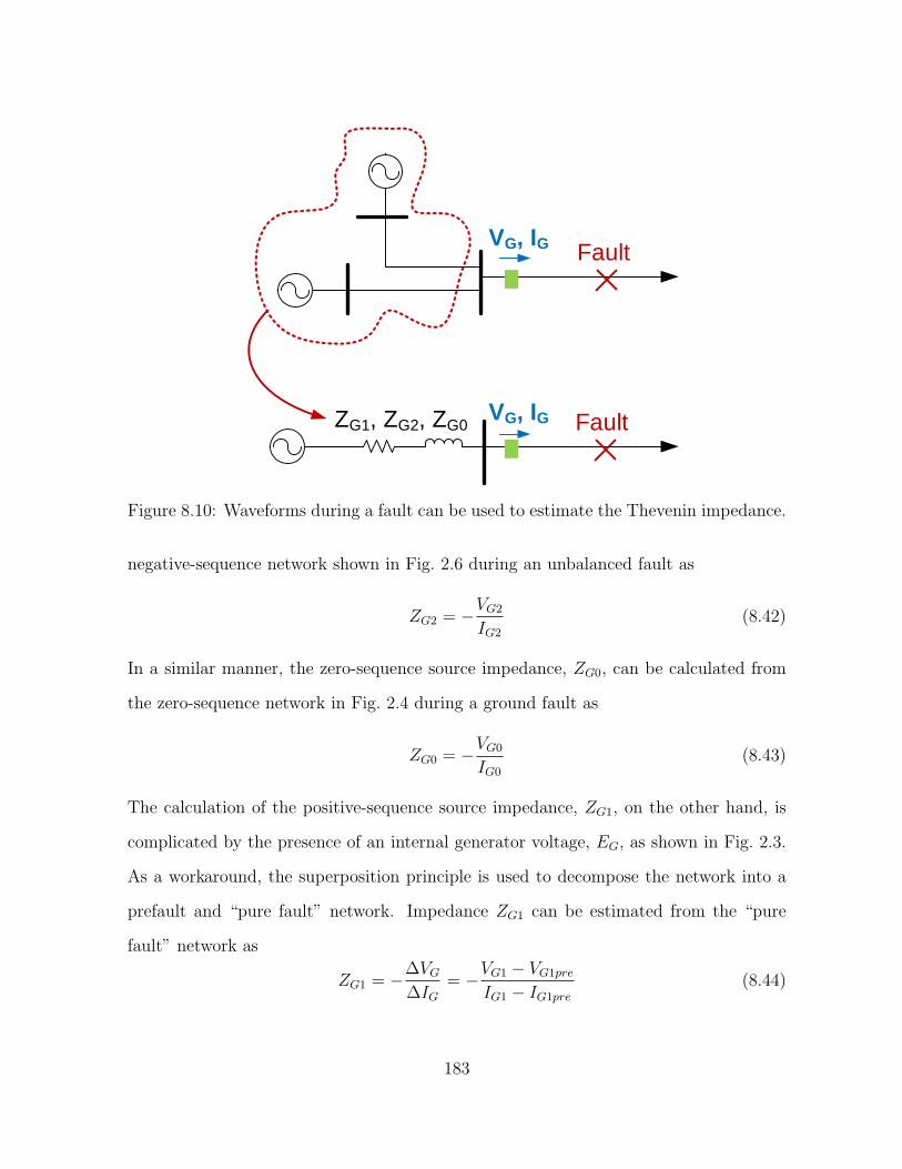
VG, IG Fault

VG, IGZG1, ZG2, ZG0 Fault

Figure 8.10: Waveforms during a fault can be used to estimate the Thevenin impedance.

negative-sequence network shown in Fig. 2.6 during an unbalanced fault as

ZG2 = −VG2

IG2

(8.42)

In a similar manner, the zero-sequence source impedance, ZG0, can be calculated from

the zero-sequence network in Fig. 2.4 during a ground fault as

ZG0 = −VG0

IG0

(8.43)

The calculation of the positive-sequence source impedance, ZG1, on the other hand, is

complicated by the presence of an internal generator voltage, EG, as shown in Fig. 2.3.

As a workaround, the superposition principle is used to decompose the network into a

prefault and “pure fault” network. Impedance ZG1 can be estimated from the “pure

fault” network as

ZG1 = −∆VG

∆IG= −VG1 − VG1pre

IG1 − IG1pre

(8.44)

183

It should be noted that ZG1 is not assumed to be equal to ZG2 and is calculated sepa-

rately using (8.44). This is because the positive-sequence impedance equals the negative-

sequence impedance in static electrical components such as lines and transformers. How-

ever, the sequence impedances are not equal to each other in rotating machines.

To demonstrate the efficacy of the above approach in estimating the Thevenin

impedance, the 69-kV test case described in Section 3.1 was used. A single line-to-

ground fault on phase A was simulated at a distance of 7.5 miles from terminal G. The

sequence voltage and current phasors recorded by the relay at terminal G before and

during the fault are as follows:

VG1=36.36∠102 kV VG2=3.25∠-78 kV VG0=9.59∠-85 kV

IG1=1.02∠56 kA IG2=0.87∠31 kA IG0=0.85∠31 kA

VG1pre=39.60∠102 kV IG1pre=0.44∠114 kA

Next, the above phasors were used to calculate the Thevenin impedances using (8.42) -

(8.44). As seen from Table 8.5, the estimated negative- and zero-sequence short-circuit

impedances matched well with the actual impedances used in the simulation model. The

positive-sequence impedance, however, show a small deviation from the actual value.

Most likely, the error stems from the constant current load model assumption in (8.44).

Table 8.5: Actual vs. Estimated Thevenin Impedances at Terminal G

ZG1 (Ω) ZG2 (Ω) ZG0 (Ω)

Actual Estimated Actual Estimated Actual Estimated

1.22+j3.55 1.11+j3.57 1.22+j3.55 1.22+j3.55 4.76+j10.20 4.76+j10.20

8.6 Verify the Power System Model

System operators usually have detailed circuit models of transmission and dis-

tribution networks in PSCAD [47], CAPE [48], OpenDSS [49], and other power system

184

software. The circuit model is useful for conducting short-circuit studies, determining

protective relay settings, and choosing the maximum rating of circuit breakers and other

power system equipment. Incorrect short-circuit model parameters can lead to erroneous

relay settings and relay misoperations, an example of which is described in [50]. As a

result, it is essential that the system model be accurate and continually updated to

reflect any system additions, repair, or modifications.

Voltage and current waveforms captured by IEDs during a fault can be used to

verify the accuracy of the system model and ensure that the model is representative

of the real world feeder. Knowing the actual fault location and estimating the fault

resistance in Section 8.4, the same fault can be replicated in the short-circuit model.

A good match between the current predicted by the short-circuit model and the actual

fault current measurement confirms the accuracy of the circuit model. This approach is

demonstrated using field event data in Section 9.4.

8.7 Summary

This Chapter presents the theory of potential applications of intelligent electronic

device data in improving power system performance and reliability. Potential applica-

tions include assessing the performance of relays, validating the zero-sequence impedance

of two- and three-terminal transmission lines, estimating the fault resistance, estimating

the Thevenin impedance, and verifying the accuracy of the short-circuit model. The

next Chapter demonstrates the above applications with actual fault event data collected

from utility transmission and distribution networks.

185

Chapter 9

Demonstration of the Benefits of Analyzing

Intelligent Electronic Device Data using Field Data

Chapter 8 presents the theory of potential applications of IED data to improve

power system reliability. The objective of this Chapter is to demonstrate those po-

tential applications using field data collected from utility transmission and distribution

networks. The contribution of this Chapter lies in analyzing five case studies in details,

sharing lessons learned, and illustrating the following applications of IED data: (a) event

reconstruction, (b) zero-sequence line impedance validation, (c) relay and circuit breaker

performance evaluation, (d) detection of incorrect power system equipment installation,

(e) fault resistance and root-cause identification, and (f) circuit model verification.

Publications:



pp. 537-557, 2014.

9.1 Case Study 1: Distribution Fault Analysis Reveals Incor-rect Line Impedance Setting

On 22 July 2010, a 24.9-kV utility distribution feeder serving 743 customers

experienced a series of complex power system faults at 9:18 pm. A digital relay [81] at

the substation reclosed twice to allow the temporary fault to clear out from the feeder.

186

Figure 9.1: Utility network diagram showing the fault location.

The reclose attempts, however, failed to clear the fault and the relay locked out, causing

all 743 customers to experience a sustained interruption for 176 minutes. During line

inspection, maintenance crew found a jumper burned open on a distribution pole at

a distance of 4.43 miles from the substation as shown in Fig. 9.1. This distance was,

therefore, reported as the actual fault location. Figure 9.2 shows the event log from the

relay. From the date and time stamp, it is evident that the relay recorded Events 3 to

7 during the fault, with Event 7 being the oldest entry. Voltage and current waveforms

of each event are shown in Figures 9.3 - 9.7. Notice how the fault type is different

for each event. Furthermore, location estimates computed by the relay during the B-G

fault match well with the reported fault location. However, the estimated and reported

fault location show a significant discrepancy for other fault types. After replacing the

jumper, the distribution feeder was re-energized by manually closing the breaker at the

substation. Unfortunately, replacing the jumper did not fix the root cause of the fault

and the feeder experienced another fault close to the previous location of 4.43 miles on

9 August 2010 as seen from Events 1 and 2 in Fig. 9.2. This Case Study reconstructs

187

Figure 9.2: Fault event log from the digital relay.

the perplexing sequence of events and solves the discrepancy in location estimates.

9.1.1 System Protection Description

The first step when reconstructing the sequence of events is to review relay set-

tings and understand its expected behavior during a fault. Figure 9.8 shows the settings

of the digital relay. Because most faults on overhead distribution lines are temporary

in nature, the relay has been programmed to allow two reclosing shots. The first re-

close open interval (79IO1) is 2.5 secs, while the second reclose open interval (79I02) is

27.5 secs. The relay resets itself when the fault disappears from the distribution feeder

for more than 70 secs. All trip operations are governed by the trip (TR) equation.

As seen from Fig. 9.8, trip occurs when the phase time-overcurrent (51T), the phase

definite-time overcurrent (50LT), the ground time-overcurrent (51NT), or the ground

definite-time overcurrent (50NLT) elements assert. Element 50LT asserts when the re-

lay measures a phase current greater than 7200A primary and the relay trips with no

intentional time delay. If the phase current is greater than 842.4A primary but less than

7200A primary, the phase time-overcurrent pickup element, 51P, asserts first and starts

timing on the U3 curve, whose equation is given as [81]:

top = TD ×[

0.0963 +3.88

M2 − 1

]

(9.1)

188

Figure 9.3: Event 7 is a BC fault at an estimated location of 5.46 miles.

Figure 9.4: Event 6 is a B-G fault at an estimated location of 4.48 miles.

189

Figure 9.5: Event 5 is a BC fault at an estimated location of 5.22 miles.

Figure 9.6: Event 4 is a B-G fault at an estimated location of 4.51 miles.

190

Figure 9.7: Event 3 is a BC-G fault at an estimated location of 5.34 miles.

where top is the relay trip time in seconds, M is a multiple of pickup and is calculated

as the ratio of the fault current to the pickup setting, and TD is the time dial setting.

After a lapse of t seconds, 51P times out and 51T asserts, causing the relay to initiate a

trip. During a ground fault, if the relay detects a residual current greater than 6408A

primary, 50NLT asserts and the relay trips instantaneously. When the residual current is

greater than 597.6A primary but less than 6408A primary, the ground time-overcurrent

pickup element, 51NP, asserts and starts timing on the U3 curve. Once 51NP times out,

51NT asserts and trips the relay.

9.1.2 Event Report Trigger Criteria

Another important step when reconstructing the sequence of events is to under-

stand what triggers IEDs to generate event reports. The relay automatically records an

event report when the trip equation (TR) asserts [81]. The 11-cycle long event report

contains voltage and current waveforms during prefault, fault, and post-fault conditions

191

Figure 9.8: Settings in the digital relay.

at 4 samples per cycle. A cosine filter processes the waveform data to remove DC offset

and other harmonic frequencies. Apart from the TR equation, digital relays also allow

system operators to monitor specific relay variables via the event report (ER) setting.

An event report is triggered when the monitored variables change state. For example,

according to the ER setting in Fig. 9.8, event reports will be triggered when the phase

time-overcurrent pickup (51P), the ground time-overcurrent pickup (51NP), or the phase

undervoltage (27) elements assert. To ensure that multiple event reports are not gener-

ated for the same fault, relay elements responsible for triggering an event report must

deassert for four cycles before they can trigger another event report.

9.1.3 Event Reconstruction

To reconstruct an accurate account of events, start with the oldest event (Event

7) recorded by the relay. Keep in mind that the waveforms record what the relay “saw”

during a fault while the digitals document the relay response during the fault. A digital

192

having a solid thick line indicates logical 1. Now, according to Fig. 9.3, the relay sees

a BC fault and a fault current magnitude of 2600A primary, which exceeds the 51P

pickup setting of 842.4A in Fig. 9.8. As a result, 51P starts timing on the U3 curve

and times out at 21:18:58.629 hours. 51T asserts and trips the relay, which prompts

the relay to record this event. Note that an earlier event showing the fault inception

is missing. After receiving the trip signal from the relay, the circuit breaker takes 2.5

cycles to interrupt the fault current (Breaker= logical 0). This additional time, known

as the breaker operating time, can be compared against manufacturer specifications to

evaluate the breaker performance. Observe that the fault current is visible for another

1.5 cycles after the circuit breaker has opened and is the response of a cosine filter to an

abrupt change in current from 2200A to 0A. At the start of the event, the relay is in

the reset state (Recloser=R). However, after issuing a trip command, the relay enters

the reclose cycle state (Recloser=C) and starts timing on the first open interval, 79OI1.

The relay starts recording Event 6 from 21:19:01.9375 hours as shown in Fig. 9.4.

By this time, 79OI1 has timed out, the relay has closed back into the circuit, and the

shot counter has increased to 1. The fault appears to have cleared out from the distri-

bution feeder. However, before the relay can reset itself (79RST = 70 secs), the feeder

experiences a B-G fault. The phase B current is 2210A primary and the residual cur-

rent is 2020A primary. Both currents are greater than the pickup settings of phase and

ground time-overcurrent elements, 51P and 51NP. The more sensitive 51NP picks up

first and triggers this event, followed by 51P as illustrated in Fig. 9.4.

When the relay starts recording Event 5, the B-G fault has developed into a BC

fault as shown in Fig. 9.5. The residual current is insignificant which causes 51NP to

drop out. 51P continues to actively time on the U3 curve and times out at 21:19:02.945

hours. The resulting trip initiates this event, and the relay enters the second open

interval, 79OI2. Since the relay has not reclosed yet, the shot count stays equal to 1.

193

The relay starts recording Event 4 after 29.28 secs as shown in Fig. 9.6. Since

79IO2 is 27.5 secs, the relay has already closed back into the circuit, and the shot counter

increases to 2. The fault appears to have cleared out from the distribution feeder.

However, before the relay can reset itself, the fault resurfaces as a B-G fault. The phase

current is 2190A primary while the residual current is 1937A primary. Both 51P and

51NP assert simultaneously and start timing on the U3 curve at 21:19:31.458 hours.

By Event 3, the fault has developed into a BC-G fault as shown in Fig. 9.7.

The primary phase and residual current magnitudes are 2820A (M =3.35) and 1793A

(M =3), respectively. Relay variables 51P and 51NP continue to actively time on the U3

curve. According to (9.1), the operating time of the phase and ground time-overcurrent

elements are 0.809 and 1.197 secs, respectively as shown in Fig. 9.9. As a result, 51T

asserts before 51NP has a chance to time out and triggers the relay to record the event.

As mentioned earlier, the circuit breaker takes an additional 2.5 cycles to open and

isolate the fault. Within this time, the fault has evolved into a three-phase fault. Since

all reclose attempts fail to clear the fault, the relay locks out (Recloser=L).

194

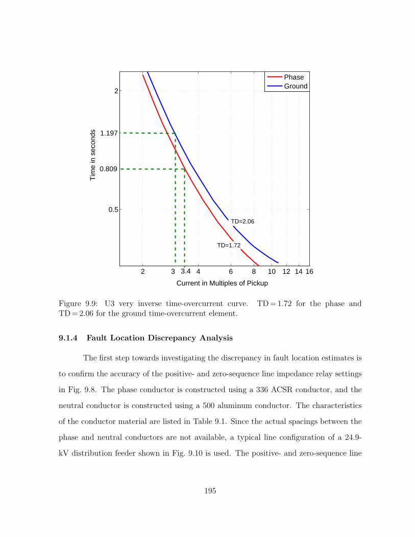
2 4 6 8 10 12 14 16

0.5

2

Current in Multiples of Pickup

Tim

e in

sec

onds

PhaseGround

TD=1.72

TD=2.06

0.809

1.197

3 3.4

Figure 9.9: U3 very inverse time-overcurrent curve. TD=1.72 for the phase andTD=2.06 for the ground time-overcurrent element.

9.1.4 Fault Location Discrepancy Analysis

The first step towards investigating the discrepancy in fault location estimates is

to confirm the accuracy of the positive- and zero-sequence line impedance relay settings

in Fig. 9.8. The phase conductor is constructed using a 336 ACSR conductor, and the

neutral conductor is constructed using a 500 aluminum conductor. The characteristics

of the conductor material are listed in Table 9.1. Since the actual spacings between the

phase and neutral conductors are not available, a typical line configuration of a 24.9-

kV distribution feeder shown in Fig. 9.10 is used. The positive- and zero-sequence line

195

Table 9.1: Conductor Data [3]

MaterialResistance GMR(Ω/mi) (feet)

Phase 336 ACSR 0.306 0.0244Neutral 500 AAC 0.206 0.0260

A

N

29'

25'

2.5' 4.5'

0.5'

B C

Figure 9.10: Line Configuration of a Typical 24.9-kV Distribution Feeder [3, 9].

impedances are calculated using Carson’s equations to be z1new =0.31+ j0.63Ω/mi and

z0new =0.55+ j1.73Ω/mi, respectively. Notice that these line impedance parameters are

different than those used by the digital relay for fault location calculations.

Next, the typical line impedance parameters of a 24.9-kV distribution feeder,

z1new and z0new, are used to estimate the distances to the fault. As seen in Table 9.2,

location estimates from all events are now close to the actual fault location. Therefore,

these findings strongly suggest that the disparity in location estimates was due to inac-

curate line impedance settings. It is recommended that the utility recalculate the line

impedance parameters and make changes as necessary.

196

Table 9.2: Location Estimates using Line Impedance Parameters of a Typical 24.9-kVDistribution Feeder having a 336 ACSR Phase and a 500 AAC Neutral Conductor isclose to the Actual Fault Location

Event Fault Type Actual Location (mi) Estimated Location (mi)

7 BC

4.43

4.72

6 B-G 4.58

5 BC 4.54

4 B-G 4.58

3 BC-G 4.57

9.1.5 Evolving Fault Analysis

Now, in addition to solving the disparity in fault location estimates, we must

also explain why the fault evolves from a BC to a B-G fault. Also, after every reclose

operation, why does the fault disappear for a few cycles and then reappear? To find a

suitable explanation, let’s take a look at the weather conditions on the day of the event.

Severe thunderstorms accompanied by rain and wind gust speeds of 40 miles per hour

were reported in the area as shown in Fig. 9.11. Most likely, high wind speeds pushed

a tree into the phase B and phase C conductors, causing conductor slapping and a BC

fault. Because of the fault, the jumper cable at 4.43 miles burned open. The high wind

speeds caused the burned open jumper cable to swing around and touch the phase and

ground conductors, resulting in a series of B-G, BC, and BC-G faults. The theory of the

tree contact fault is further supported by the recurrence of another fault on 9 August

2010 at the same location of 4.51 miles as seen from Events 2 and 1 in Fig. 9.2. Stormy

weather was reported on that day as well. The recurring fault also proves that the burned

jumper cable was the failure effect and not the root cause of the fault on 22 July 2010.

197

Figure 9.11: Stormy weather on 22 July 2010.

9.1.6 Lessons Learned

1. Any discrepancy between the reported fault location and location estimates com-

puted by the relay must be thoroughly investigated. For example, the analysis in

this case study strongly suggest that the disparity in location estimates is due to

inaccurate line impedance settings. It is recommended that the utility recalculate

the line impedance parameters and revise relay settings as needed.

2. Analysis of faults can provide insights into the root causes of faults. In this case

study, the BC fault was, most likely, caused by a tree pushing together two phase

conductors during high wind speeds. The utility is advised to trim trees near 4.43

miles to prevent future recurrence of such faults.

3. Event reports must be downloaded before being overwritten by more recent events.

For instance, an event before Event 7, which should have recorded the fault inception

198

2.34 mi 16.29 mi

VG,IGStation 1 Fault Point F VH,IH Station 2

DFR DFRZG1 ZH1

Figure 9.12: Case study 2 is a AB fault at 2.34 miles from Station 1 or 16.29 miles fromStation 2.

time, is missing. Furthermore, event reports must be thoroughly analyzed before

re-energizing the system. If event reports on 22 July 2010 were reviewed in details,

the fault on 9 August 2010 could have been prevented.

4. Events described in this case study take a longer time to unfold than the standard

event report length of eleven cycles. To visualize entire events such as these in the

future and ensure that no valuable data is lost, the utility is advised to use timers

for triggering consecutive events as described in [39].

9.2 Case Study 2: Tree Contact with a 161-kV TransmissionLine Reveals the Upstream Network Response to a Fault

This event is a line-to-line fault that occurred between phases A and B of a 161-kV

transmission line on 25 March 2012 at 03:56 pm. The transmission line is 18.63 miles long

and connects Station 1 with Station 2 as shown in Fig. 9.12. The positive- and zero-

sequence impedances of the line are ZL1=2.39+ j12.81Ω and ZL0=9.95+ j40.70Ω,

respectively. The fault was caused by a tree falling on the transmission line 2.34 miles

from Station 1 or 16.29 miles from Station 2.

199


The sequence of events can be reconstructed from the voltage and current wave-

forms captured by digital fault recorders (DFRs) at both ends of the transmission line.

The waveforms at Station 1 and Station 2 are shown in Fig. 9.13 and Fig. 9.14, respec-

tively. Both DFRs have a sampling rate of 100 samples per cycles. Before the fault,

Station 1 and Station 2 support a load current of 47A and 55A, respectively. When a

fault occurs 2.34 miles from Station 1, the DFR at Station 1 measures a fault current

of 4.8 kA in phases A and B. After 3.5 cycles, a protective relay at Station 1 initiates a

fast trip operation.

Station 2, on the other hand, continues to feed the fault for 34.5 cycles. During

the first 3.5 cycles, when both stations are feeding the fault, the DFR at Station 2 records

a current of 3.2 kA in the faulted phases. This is marked as “Part 1” in Fig. 9.14. When

Station 1 trips offline after 3.5 cycles, the fault current from Station 2 increases to 4 kA

as indicated by “Part 2” in Fig. 9.14. After 34.5 cycles, the recloser at Station 2 operates

to allow the fault to clear out on its own. The reclose interval is 2.07 seconds. The fault

is, however, permanent and the DFR measures a fault current magnitude of 4 kA when

the recloser closes back into the transmission line. This is illustrated by “Part 3” in

Fig. 9.14. The recloser eventually locks out after 3.5 cycles.

9.2.2 Fault Location

To track down the location of the permanent fault, one-ended impedance-based

fault location algorithms were applied from Station 1. Location estimates are, however,

not accurate and exceed the actual location of the fault by 1.4 miles as shown in Table 9.3.

One-ended fault location algorithms were then applied to “Part 2” and “Part 3” of the

waveforms captured at Station 2. This is because in “Part 2” and “Part 3”, only Station

2 contributes current to the fault. There is no remote infeed from Station 1 and hence,

200

Figure 9.13: Case study 2 DFR measurements at Station 1, IAF = IBF =4.8 kA.

Figure 9.14: Case study 2 DFR measurements at Station 2.

201

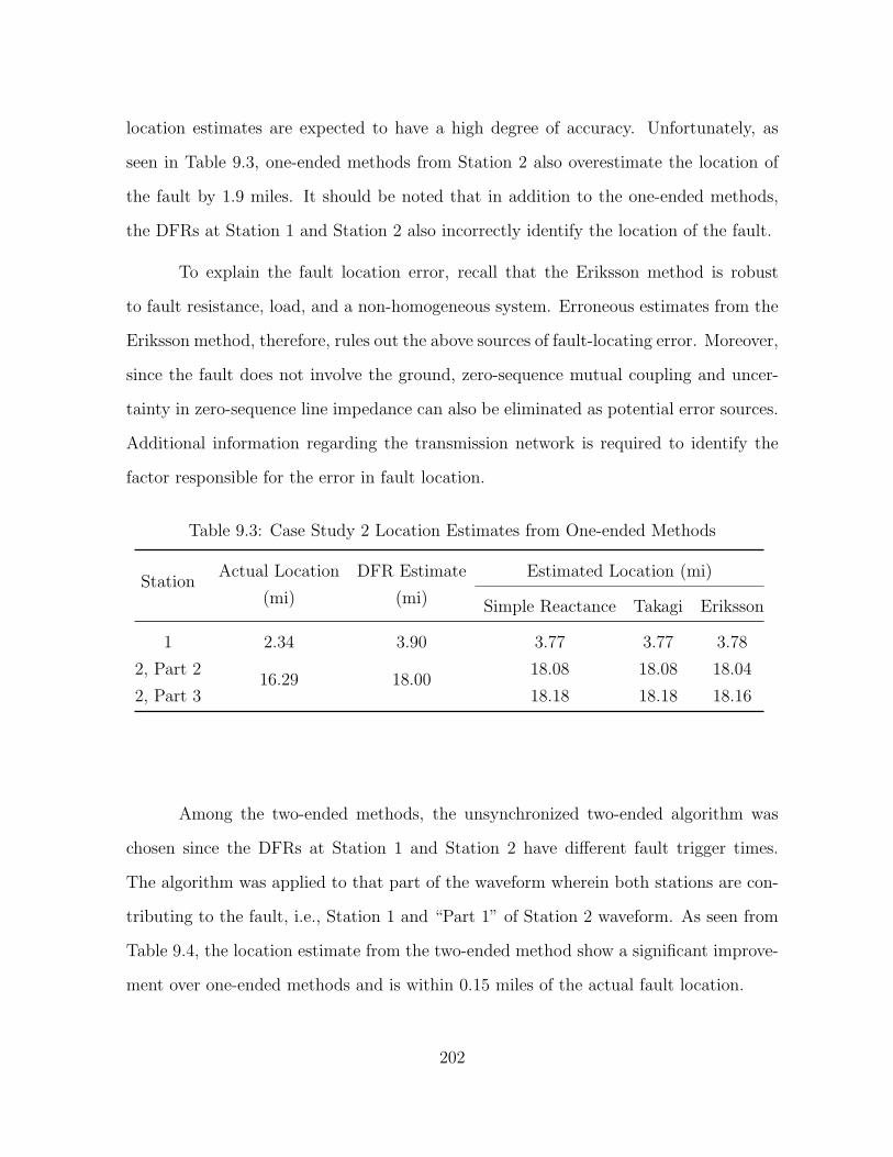
location estimates are expected to have a high degree of accuracy. Unfortunately, as

seen in Table 9.3, one-ended methods from Station 2 also overestimate the location of

the fault by 1.9 miles. It should be noted that in addition to the one-ended methods,

the DFRs at Station 1 and Station 2 also incorrectly identify the location of the fault.

To explain the fault location error, recall that the Eriksson method is robust

to fault resistance, load, and a non-homogeneous system. Erroneous estimates from the

Eriksson method, therefore, rules out the above sources of fault-locating error. Moreover,

since the fault does not involve the ground, zero-sequence mutual coupling and uncer-

tainty in zero-sequence line impedance can also be eliminated as potential error sources.

Additional information regarding the transmission network is required to identify the

factor responsible for the error in fault location.

Table 9.3: Case Study 2 Location Estimates from One-ended Methods

StationActual Location

(mi)

DFR Estimate

(mi)


Simple Reactance Takagi Eriksson

1 2.34 3.90 3.77 3.77 3.78

2, Part 216.29 18.00

18.08 18.08 18.04

2, Part 3 18.18 18.18 18.16

Among the two-ended methods, the unsynchronized two-ended algorithm was

chosen since the DFRs at Station 1 and Station 2 have different fault trigger times.

The algorithm was applied to that part of the waveform wherein both stations are con-

tributing to the fault, i.e., Station 1 and “Part 1” of Station 2 waveform. As seen from

Table 9.4, the location estimate from the two-ended method show a significant improve-

ment over one-ended methods and is within 0.15 miles of the actual fault location.

202

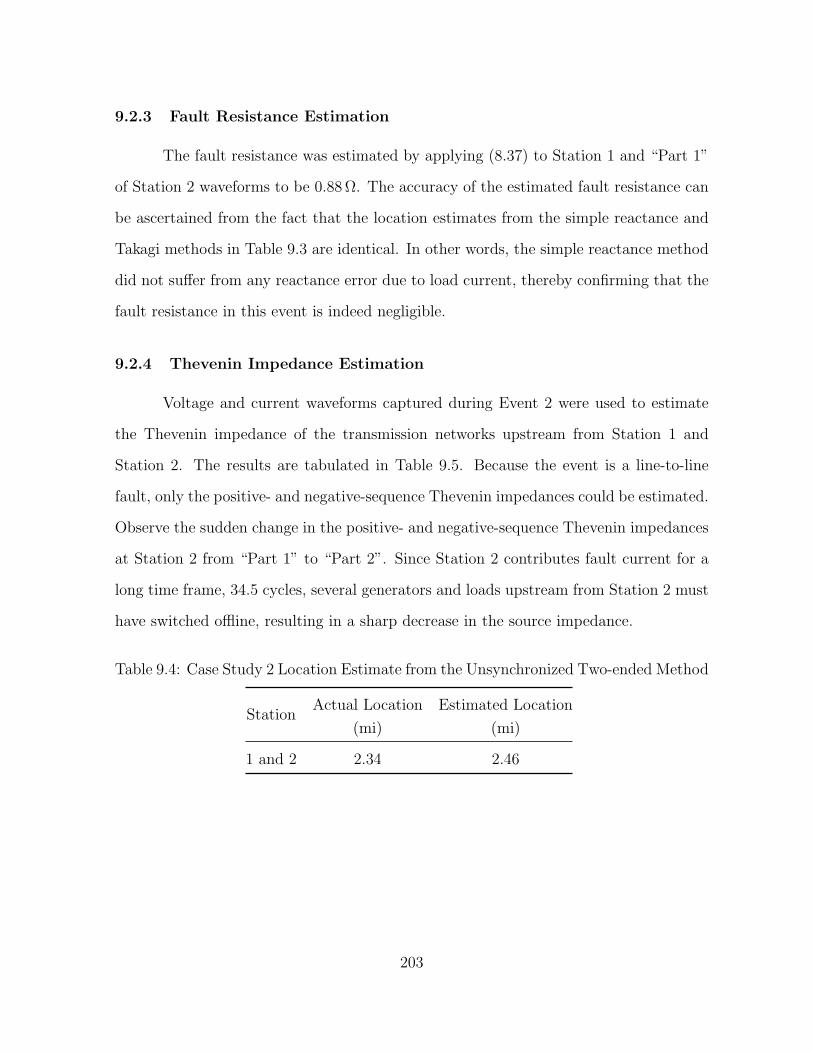
9.2.3 Fault Resistance Estimation

The fault resistance was estimated by applying (8.37) to Station 1 and “Part 1”

of Station 2 waveforms to be 0.88Ω. The accuracy of the estimated fault resistance can

be ascertained from the fact that the location estimates from the simple reactance and

Takagi methods in Table 9.3 are identical. In other words, the simple reactance method

did not suffer from any reactance error due to load current, thereby confirming that the

fault resistance in this event is indeed negligible.

9.2.4 Thevenin Impedance Estimation

Voltage and current waveforms captured during Event 2 were used to estimate

the Thevenin impedance of the transmission networks upstream from Station 1 and

Station 2. The results are tabulated in Table 9.5. Because the event is a line-to-line

fault, only the positive- and negative-sequence Thevenin impedances could be estimated.

Observe the sudden change in the positive- and negative-sequence Thevenin impedances

at Station 2 from “Part 1” to “Part 2”. Since Station 2 contributes fault current for a

long time frame, 34.5 cycles, several generators and loads upstream from Station 2 must

have switched offline, resulting in a sharp decrease in the source impedance.

Table 9.4: Case Study 2 Location Estimate from the Unsynchronized Two-ended Method


(mi)

Estimated Location

(mi)

1 and 2 2.34 2.46

203

Table 9.5: Case Study 2 Estimated Thevenin Impedance

StationPositive-sequence Impedance

(Ω)

Negative-sequence Impedance

(Ω)

1 1.85 + j14.46 3.04 + j13.66

2, Part 1 4.25 + j12.80 2.83 + j12.28

2, Part 2 6.46 + j6.29 1.72 + j7.39

2, Part 3 3.19 + j7.22 1.67 + j7.37


Analysis of faults can provide system operators with valuable clues about the

response of the upstream transmission network during a fault. For example, this case

study reveals that several critical loads upstream from the DFR at Station 2 must have

tripped offline during the fault that lasts for 34.5 cycles. In addition, the fault data

is also useful in estimating the fault resistance. Finally, the case study highlights the

superior performance of two-ended methods in estimating the fault location.

9.3 Case Study 3: Failed Line Arrestor on a 161-kV Transmis-sion Line Validates the Zero-sequence Line Impedance

On 27 April 2012, a single line-to-ground fault occurred on phase A of a 161-kV

transmission line at 00:48 am. The transmission line experiencing fault is 21.15 miles long

and connects Station 1 with Station 2 as shown in Fig. 9.15. The positive- and zero-

sequence impedances of the line are ZL1=3.18+ j16.68Ω and ZL0=15.21+ j52.45Ω,

respectively. The fault was caused by a failed line arrestor located 14.90 miles from

Station 1 or 6.25 miles from Station 2. Digital fault recorders (DFRs) at both stations

record the three-phase line-to-ground voltage and current waveforms at 100 samples per

cycle as shown in Fig. 9.16 and Fig. 9.17. Before the fault, Station 1 supports a load

current of 150A and Station 2 supports a load current of 130A. During the fault, the

204


14.90 mi 6.25 mi

DFR DFRZG1, ZG0 ZH1, ZH0

Figure 9.15: Case study 3 is a A-G fault located 14.90 miles from Station 1 or 6.25 milesfrom Station 2.

Figure 9.16: Case study 3 DFR measurements at Station 1, IAF =3.4 kA.

current magnitude in the faulted phase increases to 3.4 kA at Station 1 and to 6.1 kA at

Station 2. Note that to calculate the fault current at Stations 1 and 2, the third cycle

after fault was chosen for calculating fault current phasors.


One-ended impedance-based fault location algorithms were applied from Station

1 and Station 2 to estimate the distance to fault. As shown in Table 9.6, the location

205

Figure 9.17: Case study 3 DFR measurements at Station 2, IAF =6.1 kA.

estimates are in agreement with those estimated by the DFRs and close to the actual

location of the fault. In addition to one-ended methods, two-ended fault location meth-

ods were also used to estimate the distance to fault. Since the measurements from both

ends of the transmission line are unsynchronized due to a difference in the fault trigger

time, the unsynchronized two-ended method was used. Distance to fault was computed

to be 14.76 miles from Station 1 as shown in Table 9.7.


StationActual

Location

(mi)

DFR

Estimate

(mi)


Simple

ReactanceTakagi

Modified

TakagiEriksson

1 14.90 14.40 14.78 14.77 14.77 14.77

2 6.25 6.40 6.38 6.36 6.36 6.36

206

Table 9.7: Case Study 3 Location Estimate from the Unsynchronized Two-ended Method

Station Actual Location Estimated Location(mi) (mi)

1 and 2 14.90 14.76


Voltage and current waveforms at both ends of the line were used by (8.35) to

estimate the fault resistance to be 0.19Ω. Accurate location estimates from the simple

reactance method confirms that the fault resistance in this event was indeed negligible.


Since this case study is a ground fault, it is possible to estimate the positive-,

negative-, and zero-sequence short-circuit impedances at Station 1 and Station 2. The

estimates are listed in Table 9.8. Observe that Station 1 has a higher short-circuit

impedance and is hence, electrically weaker than Station 2. The magnitude of fault

currents contributed by each station supports this observation.

9.3.4 Zero-sequence Line Impedance Validation

Approach 1 and Approach 2 developed in Section 8.2 were used to validate the

zero-sequence line impedance. Recall that Approach 1 uses waveform data from one

207

Table 9.8: Case Study 3 Estimated Short-circuit Impedances

StationPositive-sequence Negative-sequence Zero-sequence

Source Impedance (Ω) Source Impedance (Ω) Source Impedance (Ω)

1 0.13+ j9.40 1.38+ j8.05 0.00+ j6.13

2 0.00+ j5.93 1.05+ j5.32 1.31+ j8.68

Table 9.9: Case Study 3 Setting vs. Estimated Zero-sequence Line Impedance

ApproachZero-sequence Line Impedance Error

Setting

(Ω)

Estimated

(Ω)

Magnitude

(%)

Phase Angle

(degrees)

Approach 1 (Station 1)

15.21+ j52.45

17.35+ j51.70 0.14 2.38

Approach 1 (Station 2) 18.12+ j53.97 4.24 2.38

Approach 2 (Station 1, 2) 16.93+ j53.45 2.65 1.41

end of the line and assumes a zero value of fault resistance. However, as seen in Sec-

tion 9.3.2, the fault resistance in this case study is not exactly zero. Furthermore, since

the measurements from both ends of the line are not aligned due to a difference in the

fault trigger time, this case study highlights the necessity of developing Approach 2. As

seen from Table 9.9, the estimated zero-sequence line impedance matched well with that

used by the utility as protection settings.


This case study confirms the accuracy of the zero-sequence line impedance that

was being used as a protective device setting. The fault was also found to have encoun-

tered the least resistance path to the ground. Furthermore, Station 1 was learned to be

electrically weak than Station 2.

208

Figure 9.18: Case study 4 utility circuit model in CAPE software.

9.4 Case Study 4: B-G Fault Verifies Relay Performance, Val-idates the Zero-sequence Line Impedance, and Authenti-cates the System Model

In this case study, the circuit model of the utility transmission network is available

in CAPE software [48] as shown in Fig. 9.18. The rated voltage at Substation A is 161

kV. A SEL-351R relay [10] is responsible for protecting the 23.6-mile long transmission

line that connects Substation A with Substation C. The line geometry is shown in

Fig. 9.19 and the conductor data are provided in Table 9.10. This line data is used

in Carson’s equations to calculate the positive- and zero-sequence line impedances as

ZL1=6.01+ j19.00Ω and ZL0=19.72+ j56.23Ω, respectively. On 10 January 2012,

a single line-to-ground fault on phase B occurred at a distance of 14.37 miles from

Substation A as illustrated in Fig. 9.18. The root cause of the fault is not known. The

fault, being momentary in nature, is cleared by the first shot of the SEL-351R relay.

However, the same fault reappears in the circuit after 15 minutes as seen from the event

log in Fig. 9.20. The SEL relay operates again to allow the temporary fault to clear from

the circuit. During the entire duration, the relay records four events, whose voltage and

current waveforms are shown in Figures 9.22 - 9.25. This Section uses the waveform

209

A

S1

62.15'

51.15'

16' 16'

8.56' 8.56'

S2

B C

Figure 9.19: Overhead transmission line spacing in feet.

Table 9.10: Conductor Data

Material Resistance Diameter GMR

(Ω/mi) (inch) (feet)

Phase Conductor 397,500 26/7 ACSR 0.2537 0.7836 0.0265

Shield Wire 3/8 A HSS 5.6500 0.3600 0.0120

data to reconstruct the sequence of events, estimate the fault location, assess relay

performance, estimate the fault resistance, validate the zero-sequence line impedance,

and verify the accuracy of the system model.

9.4.1 System Protection Description

The settings of the SEL-351R relay are shown in Fig. 9.21. The relay is pro-

grammed to perform three automatic reclosures. The first reclose open interval (79IO1)

is 10 cycles, the second reclose open interval (79I02) is 1800 cycles, and the third reclose

open interval (79IO3) is 3600 cycles. The relay resets itself when the fault disappears

210

Figure 9.20: SEL-351R fault event history.

from the transmission feeder for more than 900 cycles. A trip occurs when the phase

instantaneous element with directional control (67P1T), the phase time-overcurrent

(51PT) element, the ground instantaneous element with directional control (67G1T),

or the ground time-overcurrent (51NT) element asserts as evident from the TR equation

in Fig. 9.21. Now, 67P1T asserts when the phase current is greater than 1048.80A pri-

mary and the relay trips with no intentional time delay. On the other hand, if the phase

current is between 540A primary and 1048.80A primary, the phase time-overcurrent

pickup element, 51P, picks up and starts to time on the U3 curve given by (9.1). When

51P times out, 51T asserts and causes the relay to initiate a trip. During a ground fault,

if the relay detects a ground current greater than 560.40A primary, element 67G1T as-

serts and the relay trips instantaneously. When the ground current is greater than 288A

primary but less than 560.40A primary, the ground time-overcurrent pickup element,

51GP, asserts and starts timing on the U3 curve. Once 51GP times out, 51GT asserts

211

Figure 9.21: Settings in the SEL-351R relay.

and trips the relay. It is important to note that 67P1T and 67G1T are disabled for shot

1 as specified by the trip equation in Fig. 9.21. Logical operator ! indicates a NOT func-

tion, operator * indicates a AND function, and SH1=1 when the relay is at shot= 1.

In other words, during shot 1, the relay will trip only for 51P1T and 51G1T elements.

9.4.2 Event Report Trigger Criteria

According to the ER setting in Fig. 9.21, the SEL-351R relay records an event re-

port when the trip equation (TR) asserts or when the phase and ground time-overcurrent

212

elements, 51P and 51G, pick up. The operator / indicates the rising edge of the element.

The 16-cycle long event report contains voltage and current waveforms during prefault,

fault, and post-fault conditions at 16 samples per cycle.


To build an accurate account of the sequence of events, start with the oldest

event recorded by the relay in Fig. 9.22. The load current supported by the substation

is 116A. During the phase B-to-ground fault, the phase and the ground fault current

magnitudes increase to 2360A and 2300A, respectively. As a result, both 67P1T and

67G1T assert simultaneously at 12:44:38.413 hours and the relay send a trips signal to

the circuit breaker. Observe that the circuit breaker takes an additional three cycles to

interrupt the current as shown in Fig. 9.22. This breaker operate time can be compared

against manufacturer specifications to verify the breaker performance. After receipt of

the circuit breaker open status, the relay starts timing on the first open interval, 79OI1.

When 79OI1 times out, the shot counter increases to 1 and the circuit breaker

closes back into the circuit at 12:44:38.885 hours as shown by Event 3 in Fig. 9.23.

The fault, however, is still present in the circuit and the relay measures a phase and

ground current of 2860A and 2811A, respectively. Since the operation of the 67P1T

and 67G1T elements are suspended in shot 1, the ground time-overcurrent element picks

up at 12:44:38.893 hours and starts timing on the U3 curve. The phase time-overcurrent

element also picks up at 12:44:38.897 hours and triggers this event. According to (9.1),

the operating time of the phase and ground time-overcurrent elements are 0.316 and

0.203 secs, respectively. As a result, 51GT asserts before 51P has a chance to time out

and issues a trip signal to the circuit breaker. Because the SEL relay records only 16

cycles of waveform data, the opening of the circuit breaker is not shown.

By the time the SEL-351R relay starts recording Event 2 at 12:59:41.476 hours,

213

Figure 9.22: Event 4 voltage and current waveforms at shot= 0.


214



215

the circuit breaker has already closed back into the circuit. The fault has cleared and the

phase B current has returned back to normal load current levels as shown in Fig. 9.24.

The relay has also reset itself since the fault was absent from the transmission network

for more than 900 cycles. Unfortunately, the fault reappears on phase B at 12:59:41.526

hours. Element 67G1T asserts immediately and trips the circuit breaker. The relay

starts timing on the first open interval, 79OI1.

When 79OI1 times out, the circuit breaker closes back into the circuit, and the

shot counter increases to 1. The fault, however, persists, and the relay measures a phase

and a ground current of 3380A and 3340A, respectively. Since the operation of the

67P1T and 67G1T elements are suspended for shot 1, both the phase and the ground

time-overcurrent elements pick up at 12:59:41.995 hours and start timing on the U3

curve. The more sensitive ground time-overcurrent, 51GT, times out before its phase

counterpart, 51PT, and trips the circuit breaker at 12:59:42.186 hours. No other event

reports are available. Therefore, it is not clear whether this shot of the relay removed

the fault or whether the relay eventually locked out to isolate the permanent fault.

9.4.4 Relay Performance Assessment

The Section aims to assess the performance of the SEL-351R relay and to deter-

mine whether relay operating times are within set time limits. The goal is to compare

the expected time of operation with the actual relay operating time.

(a) Assessment of Trip Time during Shot 1 in Event 3

During this shot, the relay measures a ground fault current magnitude of 2811A

primary (2811/CTR=23.43A secondary). The actual operating time is the time dif-

ference between assertion of 51GP at 12:44:38.893 hours and assertion of 51GT at

12:44:39.072 hours, and is calculated to be 0.179 secs.

216

Figure 9.26: Functional specifications of the SEL-351R relay [10].

Next, when calculating the expected operating time of the relay, the functional

specifications of the relay must be taken into consideration. According to Fig. 9.26, 51G

has a pickup accuracy of ± 3% of setting ± 0.05A. Therefore, for a pickup setting of

2.40A secondary, the pickup accuracy equals ± 0.12A. This means that when the actual

fault current is 23.43A secondary, 51GT can assert when the current is between 23.31A

and 23.55A secondary (23.43± 0.12A).

Suppose the relay picks up at 23.31A secondary (M =9.71). Using (9.1), the

operating time of the relay is 0.204 secs. As per Fig. 9.26, 51G has a curve timing

accuracy of ± 4% of the operating time and ± 1.5 cycles. For an operate time of 0.204

secs, the curve timing accuracy equals 0.0332 secs (4%×0.204± 0.025 secs). Therefore,

the relay is expected to operate within 0.1708 and 0.2372 secs (t1=0.204± 0.0332 secs).

Alternatively, suppose the relay picks up when the fault current is 23.55A sec-

ondary (M =9.81). From (9.1), the operating time of the relay is solved to be 0.203

secs. The curve timing accuracy for this operate time is calculated to be 0.0331 secs

(4%×0.203± 0.025 secs). Therefore, the relay will operate within 0.1699 and 0.2361 secs

(t2=0.203± 0.0331 secs).

The final time window, tfinal, that accounts for both pickup and curve timing

accuracy can be calculated as Min (t2)<tfinal <Max (t1) or 0.1699<tfinal < 0.2372 secs.

217

The actual trip time of 0.179 secs falls within the expected window of operation, thereby

validating the relay first shot.

(b) Assessment of Trip Time during Shot 1 in Event 1

During shot 1 in Event 1, the relay measures a ground fault current magnitude

of 3340A primary (3340/CTR=27.83A secondary). Following the procedure outlined

in the previous section, the relay is expected to operate within 0.1528 and 0.2184 secs.

From Fig. 9.25, 51GP asserts at 12:59:41.995 hours while 51GT asserts at 12:59:42.186

hours. Therefore, the actual operating time of 0.191 secs lies within the expected window

of operation and hence, the relay performs as expected.


Distance to the fault was computed by applying one-ended fault location algo-

rithms such as the simple reactance, Takagi, and Novosel et al. methods to all the four

events. Notice that Event 4 and Event 2 are short-duration faults with a significant

DC offset. Therefore, the third cycle after fault inception was chosen to compute the

fault current phasors and minimize any error due to DC offset. Results tabulated in

Table 9.11 indicate that the fault location estimates from the one-ended algorithms are

in good agreement with those estimated by the SEL 351-R relay and are close to the

actual fault location.

218


Event Actual Location SEL-351REstimated Location (mi)

(mi) Estimate (mi) Simple Reactance Takagi Novosel et al.

4

14.37

14.08 14.18 14.20 14.17

3 14.18 14.08 14.07 14.07

2 14.43 14.45 14.46 14.45

1 14.65 14.65 14.63 14.62

Table 9.12: Estimated Values of Fault Resistance in Case Study 4

Event Fault Resistance (Ω)

4 0.02

3 0.06

2 0.90

1 1.70


Using voltage and current waveforms from one end of the line and the known fault

location, Approach 1 described in Section 8.4 was used to estimate the fault resistance.

As seen from Table 9.12, the fault resistance is expected to lie between 0.02 and 1.7Ω.


Since Events 4 through 1 describe an unbalanced fault with a return path to the

ground, the waveforms captured in those events can be used to estimate the positive-,

negative-, and zero-sequence Thevenin impedances upstream from the SEL-351R relay.

The estimated Thevenin impedances were then compared with the circuit model in

CAPE to gauge the accuracy of estimation. As seen in Table 9.13 and Table 9.14, the

reactance component of the Thevenin impedances are a good fit with those obtained

219

from the circuit model. The resistive component, on the other hand, absorbs the error

and hence, show greater variations.

9.4.8 Zero-sequence Line Impedance Validation

Since the fault described in Events 4 through 1 involve a return path through the

ground, it is possible to use the event data captured by the SEL-351R relay to verify the

zero-sequence line impedance. Because data from only one end of the line is available,

Approach 1 described in Section 8.2 was used and the results are shown in Table 9.15.

The magnitude and phase angle errors were calculated using (8.14). From Table 9.15,

it can be concluded that the estimated zero-sequence line impedance matched well with

that used as relay setting.

9.4.9 Short-circuit Model Verification

Event reports captured by the SEL 351-R recloser can be used to confirm the

accuracy of the circuit model in CAPE. As described in Section 8.6, the approach is to

replicate the actual fault in the circuit model and compare the resulting short-circuit

current with actual field measurements. As an example, Event 1 was recreated by

simulating a B-G fault in the CAPE circuit model at the known location of the fault, i.e.,

14.37 miles from the substation as shown in Fig. 9.18. The fault resistance estimated

in Table 9.12, RF =0.02Ω, was used. Comparison between the short-circuit current

in CAPE and the fault current measured by the SEL relay in Event 1 is shown in

Fig. 9.27. The currents match well once the DC offset decays out after the third cycle.

Comparison between short-circuit currents in CAPE and SEL relay measurements for

all the remaining events are presented in Table 9.16. Results indicate that the circuit

model in CAPE is representative of the actual transmission network.

220

Table 9.13: Actual vs. Estimated Positive- and Negative-sequence Thevenin Impedances

EventPositive-sequence Impedance (Ω) Negative-sequence Impedance (Ω)

Circuit Model Estimated Circuit Model Estimated

4

2.82+ j17.90

3.62+ j17.35

2.91+ j18.03

2.94+ j17.09

3 1.90+ j18.36 3.18+ j16.84

2 4.12+ j17.31 3.13+ j17.08

1 1.43+ j18.77 3.71+ j17.11

Table 9.14: Actual vs. Estimated Zero-sequence Thevenin Impedance

EventZero-sequence Thevenin Impedance (Ω)

Circuit Model Estimated

4

5.29+ j30.72

4.88+ j29.75

3 5.20+ j29.59

2 5.17+ j29.70

1 5.89+ j29.78

Table 9.15: Setting vs. Estimated Zero-sequence Line Impedance

EventZero-sequence Line Impedance (Ω) Error

Relay Setting Estimated Magnitude (%) Phase Angle (degrees)

4

19.72+j56.22

24.06+j55.03 0.79 4.29

3 23.60+j54.30 0.63 4.16

2 21.84+j56.75 2.05 1.72

1 26.12+j57.37 5.79 5.15

221

Figure 9.27: Fault current in the circuit model matches well with that measured by theSEL-351R relay in Event 1.

Table 9.16: Short-circuit Current in CAPE vs. Actual Measurements from SEL-351R

Event Actual Location Estimated LocationFault Current (kA)

(mi) (mi) SEL-351R CAPE

1

14.37

14.18 2.36 2.19

2 14.08 2.30 2.19

3 14.45 2.34 2.18

4 14.65 2.33 2.17

222


Analysis of this event successfully reconstruct the sequence of events and verifies

the performance of the relay. In addition, the fault data was used to validate the zero-

sequence line impedance setting in the SEL-351R relay. Furthermore, the fault event

data was used to estimate the fault resistance and confirm that the circuit model is

representative of the actual transmission network.

9.5 Case Study 5: Lightning Strike on a 161-kV TransmissionLine Reveals Incorrect CT Polarity and Missing Phase CT

On 21 January 2012, a 161-kV transmission line experienced a three-phase fault

due to a lightning strike at 5.86 miles from Station 1 or 17.53 miles from Station 2 as

shown in Fig. 9.28. The transmission line is 23.39 miles long and has a positive- and zero-

sequence impedance of ZL1=2.85+ j18.22 Ω and ZL0=16.80+ j60.89 Ω, respectively.

A digital fault recorder at Station 1 captures the voltage and current waveforms at 100

samples per cycle as shown in Fig. 9.29. Notice that the phase A current waveform is

missing. The prefault current at Station 1 is 150A while the fault current is 11 kA. The

three-phase voltage and current waveforms at Station 2 are recorded by a DFR having a

sampling rate of 96 samples per cycle and are shown in Fig. 9.30. The prefault current

is 200A while the fault current magnitude is 3.6 kA.


5.86 mi 17.53 mi

DFR DFRZG1 ZH1

Figure 9.28: Case study 5 is a ABC fault at 5.86 miles from Station 1 or 17.53 milesfrom Station 2.

223

Figure 9.29: Case study 5 voltage and current waveforms at Station 1. Phase A currentis missing.

Figure 9.30: Case study 5 voltage and current waveforms at Station 2.

224


When one-ended fault-locating algorithms are applied to Station 1 data, distance-

to-fault estimates are close to the actual location of the fault as seen in Table 9.17.

Estimates from one-ended algorithms applied to Station 2 data are also close to the actual

fault location. However, it is puzzling to observe that the distance estimates are negative.

Most likely, the CT has been installed with a reverse polarity and hence, measures current

in a direction opposite to the fault as illustrated in Fig. 9.31. The reverse CT polarity

is further evident if one looks closely at the positive- and negative peak of the voltage

and current waveforms recorded at Station 2. As shown in Fig. 9.30, when current in a

particular phase has a positive peak, the corresponding voltage has a negative peak, i.e.,

a 180-degree phase shift. Therefore, the negative location estimate can be interpreted as

17.80 miles upstream with respect to the Station 2 DFR direction shown in Fig. 9.31. It

is also interesting to observe that the DFR at Station 2 underestimated the fault location

by a mile. It is possible that the incorrect CT polarity or inaccurate line parameters

contributed to the fault location error.

Table 9.17: Location Estimates from One-ended Methods


(mi)

DFR Estimate

(mi)


Simple Reactance Takagi Eriksson

1 5.86 5.90 5.96 5.96 5.96

2 17.53 16.60 -17.70 -17.80 -17.60

Because the sampling rate of the DFRs at Station 1 and Station 2 are not equal,

the unsynchronized two-ended method described in Section 2.2.2 was chosen to estimate

the fault location. The missing phase A current at Station 1 did not allow for the

225


5.86 mi 17.53 mi

DFR DFRZG1 ZH1

Figure 9.31: Negative distance estimate from Station 2 indicates that the meter directionis reversed.

calculation of sequence components. However, since the event is a balanced three-phase

fault, it was possible to use phase components instead of symmetrical components. The

reverse polarity of the CT at Station 2 was also taken into account. As seen from

Table 9.18, the location estimate from the two-ended method is close to the actual fault

location.

Table 9.18: Case Study 5 Location Estimate from Two-ended Methods


(mi)

Estimated Location

(mi)

1 and 2 5.86 5.71


Voltage and current waveforms at both ends of the line were used in (8.40) to

estimate the fault resistance as 0.26Ω. The accuracy of the estimated fault resistance

can be ascertained from the fact that the simple reactance method in Table 9.17 did not

suffer from a reactance error due to load current. The absence of the reactance error

suggests that the fault resistance in this event is indeed negligible.

226


Since Event 4 is a balanced three-phase fault, only the positive-sequence Thevenin

impedance could be estimated from the fault data as shown in Table 9.19. Results

indicate that Station 2 is electrically weaker than Station 1. Although the circuit model

is not available, judging from the fault currents contributed by each station, impedance

estimates are likely to be accurate.

Table 9.19: Estimated Positive-sequence Source Impedances

StationSource Impedance

(Ω)

1 0.46 + j3.66

2 2.25 + j11.38


Analysis of fault data can reveal incorrect setup of power system equipment or

incorrect field wiring that was missed during field commissioning tests. Results of the

analysis can be used to take corrective action and avoid future misoperations. For exam-

ple, this event shows that the CT at Station 2 was installed with an incorrect polarity.

As a result, the direction of the current was reversed and can affect the reliability and

performance of directional relays. Furthermore, the phase A current at Station 1 was

missing. It is possible that the phase CT has not been connected to the DFR and can

result in loss of valuable information. The fault was observed to have encountered the

least resistance path to the ground, which coincides with the root cause of the fault.

Finally, Station 2 was learned to be electrically weaker than Station 1.

227

9.6 Summary

In summary, this Chapter uses field data collected from utility transmission and

distribution networks to demonstrate the following benefits of analyzing fault data:

• Assess the Relay and Circuit Breaker Performance

Intelligent electronic devices record what they “see” during a fault in the form of

an event report. These reports can be used to assess the performance of relays and

circuit breakers as demonstrated in Case Study 4.

• Validate the Line Impedance

Event reports are a valuable resource for validating the line impedance settings

in relays. For example, Case Study 2 and Case Study 4 illustrates how a single

or double line-to-ground fault event can be used to validate the zero-sequence

impedance of a transmission line. Case Study 1, on the other hand, reveals a

possible inaccuracy in the positive-sequence line impedance.

• Estimate the Fault Resistance

Fault data captured at one or both ends of the line can be used to estimate the

fault resistance. Interpretation of this value is useful in determining the root cause

of the fault. Knowing the fault resistance value also plays a significant role when

verifying the accuracy of the circuit model as demonstrated in Case Study 4.

• Estimate the Thevenin Impedances

Estimating the Thevenin impedance during a fault provides valuable feedback

about the state of the transmission network upstream from the monitoring location.

Case study 2 is an excellent example. During the fault, which lasts for 34.5 cycles,

the estimated Thevenin impedances were shown to decrease suddenly. This change

suggests that several critical loads upstream from the monitoring location must

have tripped offline during this long event.

228

• Confirm the Accuracy of the System Circuit Model

Another application of analyzing fault data lies in verifying the accuracy of the

circuit model as established in Case Study 4.

• Detect Incorrect Installation of Power System Equipment

Analysis of fault data can reveal incorrect setup of power system equipment or

incorrect field wiring that was missed during field commissioning tests. Results of

the analysis can be used to take corrective action and avoid future misoperations.

For example, Case Study 5 detects a CT with incorrect polarity and a digital fault

recorder with a missing measurement channel.

229

Chapter 10

Conclusion

The overall objective of this dissertation is to describe the theory of impedance-

based fault location algorithms, identify the sources of fault location error, propose

solutions to overcome those error sources, and share lessons learned from analyzing

intelligent electronic device data. The goals are to reduce system downtime, prevent

protection system misoperations, and improve power quality.

To achieve the above objective, Chapters 2 and 3 present the theory of one- and

two-ended impedance-based fault location algorithms and identify their strengths and

weaknesses. The simple reactance method is the most straightforward of all fault location

algorithms. The accuracy of this method, however, deteriorates due to fault resistance,

load current, and remote infeed in a non-homogeneous system. Subsequent fault-locating

algorithms address the above sources of error. For example, the Takagi method is robust

to load but sensitive to remote infeed. The modified Takagi and Eriksson methods use

source impedance parameters to eliminate the fault location error caused by load and

remote infeed. Additional sources of error that compromise the accuracy of one-ended

algorithms in locating single line-to-ground faults are mutual coupling in double-circuit

transmission lines and an uncertain value of zero-sequence line impedance. Two-ended

fault-locating algorithms use measurements from both ends of a transmission line to

overcome the short-comings of one-ended methods and are an attractive solution for

tracking down the exact location of a fault. Unfortunately, measurements captured

at the remote end of the line are not always available. Furthermore, both one- and

two-ended algorithms require the input of voltage and current phasors to estimate the

230

distance to a fault. Due to operational constraints or equipment malfunction, voltage

measurements may not be available. To perform fault location even in the absence of

voltage measurements, Chapter 4 develops current-only fault location algorithms. The

discussion so far suggests that data availability is a key criteria in selecting the best

approach for fault location.

Another key criteria in selecting the best approach for fault location is the appli-

cation scenario. As an example, Chapter 3 demonstrates that two-ended algorithms are

not suited to locate faults in three-terminal lines. In contrast, one-ended fault locating

algorithms applied from one of the three terminals pinpoints the exact location of the

fault. Two-ended fault location algorithms fail not because of limitations in the algo-

rithms but because it was not meant for use in a three-terminal line. Moreover, one-ended

algorithms designed for application to a distribution feeder assume a radial feeder where

the power flows unidirectionally from the substation to the end users. With increased

penetration of distributed generators to the grid, this assumption is violated. Distributed

generators also contribute to the fault and adversely affect the accuracy of impedance-

based algorithms as illustrated in Chapter 5. In such scenarios, improved algorithms

developed in Chapter 6 that account for the fault current contribution from distributed

generators in the fault location computation must be applied. From this discussion, it

is evident that system operators need to be aware of the application scenario, identify

possible error sources, and then choose the algorithm most robust to those error sources.

Therefore, based on the analysis conducted in this dissertation, the following cri-

teria are recommended for selecting the most suitable fault location algorithm: (a) data

availability, and (b) fault location application scenario. This is illustrated in Fig. 10.1.

The fault location suite provides the user with several choices, including one- and two-

ended impedance-based fault location algorithms, current-only fault location algorithms,

and fault location algorithms that account for distributed generation. Depending on

231

Figure 10.1: Graphical illustration of the objectives of this dissertation.

data availability and the application scenario, the user can apply the best fault-locating

approach to the intelligent electronic device (IED) data and determine the location to

a fault. The same IED data can be used for other applications that improve power

system reliability as described in Chapters 8 and 9. Potential applications include as-

sessing relay performance, evaluating the performance of circuit breakers, validating the

zero-sequence impedance of multi-terminal transmission lines, estimating the fault resis-

tance, tracking the response of the upstream transmission network, and confirming the

accuracy of the system model.

Key Technical Contributions:

• Provided a comprehensive theory of one- and two-ended impedance-based fault

location algorithms, identified the input data requirement and the strengths and

232

weaknesses of each algorithm.

• Recommended the following criteria for choosing the most suitable fault location

algorithm: data availability and application scenario.

• Developed current-only fault location algorithms that use either the fault current

magnitude or the fault current phasor to estimate the distance to a fault.

• Demonstrated the adverse impact of distributed generators on impedance-based

fault location algorithms.

• Proposed an algorithm that improves fault location accuracy in the presence of

distributed generators.

• Modeled a high-resolution time-domain model of a fixed-speed wind turbine that

includes a detailed representation of tower shadow and wind shear components.

• Verified the suitability of using the IEC 60909-0 Standard in calculating protective

device settings in networks interconnected with distributed generation.

• Proposed algorithms to validate the zero-sequence impedance of two- and three-

terminal transmission lines using unsynchronized measurements.

• Demonstrated the potential of intelligent electronic data in assessing relay perfor-

mance, estimating the fault resistance and identifying the root cause of a fault,

tracking the response of the upstream transmission network, and confirming the

accuracy of the system circuit model.

233

Appendix

234

Appendix A

Line Constant Calculation

Positive- and zero-sequence line impedances play a critical role when computing

the distance to a fault. This Chapter explains how to solve for line constants from the

arrangement of phase and neutral conductors, and conductor data.

A.1 Self and Mutual Line Impedance

The following three models are commonly used to calculate the self and mutual

impedances of an overhead line:

A.1.1 Full Carson’s Model

The Full Carson’s model assumes the earth to be an infinite, homogeneous solid

with a constant resistivity. A method of images is used wherein every conductor above

the ground has a fictitious image conductor at the same distance below the ground as

illustrated in Fig. A.1. The self and mutual impedances of the line, Zii and Zik, are

given by [3, 82]

Zii = RCi + 4ωPG+ j

[

2ωG ln(ri

GMRi

) + 2ωG ln(2hi

ri) + 4ωQG

]

Ω/mi

Zik = 4ωPG+ j

[

2ωG ln(Dik

dik) + 4ωQG

]

Ω/mi

(A.1)

235

i k

i’ k’

dik

DikDii

hiθ

Figure A.1: Conductors and their images in Carson’s model.

where P and Q are complex correction factors defined as

P =π

8− 1

3√2k cos θ +

k2

16cos 2θ

(

0.6728 + ln2

k

)

+k2

16θ sin 2θ +

k3 cos 3θ

45√2

− πk4 cos 4θ

1536

Q =− 0.0386 +1

2ln

2

k+

1

3√2k cos θ − πk2 cos 2θ

64+

k3 cos 3θ

45√2

− k4

384θ sin 4θ (A.2)

− k4

384cos 4θ

(

1.0895 + ln2

k

)

.

Constants k and θ in (A.2) can be calculated as

k = 1.713× 10−3hi

√

f

ρ

θ = 0

for self-impedance

236

k = 0.8565× 10−3Dik

√

f

ρ

θ = cos−1

(

hi + hk

Dik

)

for mutual impedance.

Notations used in the above equations are defined as follows:

Zii Self-impedance of conductor i (Ω/mi)

Zik Mutual impedance between conductors i and k (Ω/mi)

RCi Internal resistance of conductor i (Ω/mi)

ω System angular frequency (rad/s)

f System frequency (Hz)

G Constant = 0.1609347× 10−3(Ω/mi)

ri Radius of conductor i (ft)

GMRi Geometric mean radius of conductor i (ft)

ρ Earth resistivity (Ω/m)

dik Distance between conductors i and k (ft)

Dik Distance between conductor i and image k′ (ft)

Dii Distance between conductor i and its own image i′ (ft)

hi Height of conductor i above the ground (ft)

hk Height of conductor k above the ground (ft)

θ Angle between Dii and Dik

A.1.2 Modified Carson’s Model

The modified Carson’s model, popularly used for power frequency calculations,

approximates the full Carson’s model by retaining only the first term of correction factor

237

P and the first two terms of correction factor Q. As a result, the calculation of self and

mutual impedance terms simplify down to [3, 82]

Zii = RCi + 0.00159f + j0.004657f log10

2160

√

ρ

f

GMRi

Ω/mi

Zik = 0.00159f + j0.004657f log10

2160

√

ρ

f

dik

Ω/mi .

(A.3)

A.1.3 Deri Model

Equations proposed by Dubanton and implemented by Deri use simple expres-

sions to calculate the line impedances which are valid over a wide frequency range. The

earth is replaced by a superconducting earth current return plane located at a complex

depth p below the ground. Self and mutual line impedances are given as [82, 83]:

Zii = RCi + jωµ0

2πln

(

2hi + 2p

ri

)

Ω/mi

Zik = jωµ0

2πln

√

(hi + hk + 2p)2 + d2ik√

(hi − hk)2 + d2ik

Ω/mi .

(A.4)

The complex penetration depth p in (A.4) can be calculated as

p =3.28084√jωµ0σ

. (A.5)

where µ0 is the permeability of free space (4π×10−7 H/m) and σ is the earth conductivity

in units of S/m.

238

A.2 Phase Impedance Matrix

After using one of the three earth return models in Section A.1 to calculate the

self and mutual line impedances, construct a primitive impedance matrix, Zprimitive, of

size N ×N , where N is the total number of phase and neutral conductors. For example,

Zprimitive for a three-phase four wire system shown in Fig. A.2 can be written as [3]

Zprimitive =

Zaa Zab Zac Zan

Zba Zbb Zbc Zbn

Zca Zcb Zcc Zcn

Zna Znb Znc Znn

Ω/mi

Here a, b, and c are phase conductors, and n is the neutral conductor. Denoting phase

and neutral conductors by subscripts p and n, respectively, Zprimitive can be partitioned as

Zprimitive =

[Zpp] [Zpn]

[Znp] [Znn]

Ω/mi

To eliminate the neutral conductor, apply Kirchhoff’s circuit law to write the voltage

drop across the feeder in Fig. A.2 as

[Vabcg]

[Vng]

=

[V′

abcg]

[V′

ng]

−

[Zpp] [Zpn]

[Znp] [Znn]

×

[Iabc]

[In]

(A.6)

where Vig is the voltage between conductor i and the ground at one end of the line, V′

ig

is the voltage between conductor i and the ground at the other end of the line, and Ii

239

Vag

Zaa

Zbb

Zcc

Vbg

Vcg

Vng

Ia

Ic

Ib

Znn

+

-

In

V’ag

V’bg

V’cg

Zab

Zbc

Zcn

Zac

ZanZbn

V’ng

+

-

Figure A.2: Kron reduction assumes a perfectly grounded neutral [3].

is the current through conductor i. If the neutral is assumed to be perfectly grounded

to the earth, Vng and V′

ng can be set to zero. As a result, (A.6) can be rearranged and

simplified to obtain a phase impedance matrix, Zabc, of size M × M , where M is the

total number of phase conductors as:

[Zabc] = [Zpp]− [Zpn][Znn]−1[Znp] Ω/mi (A.7)

This process of eliminating the neutral conductor is known as Kron reduction.

A.3 Positive- and Zero-sequence Line Impedances

Although the phase impedance matrix calculated in Section (A.2) is the most

accurate representation of an overhead feeder, the impedance-based fault location al-

gorithms characterize a feeder in terms of its positive- and zero-sequence components.

240

Assuming a transposed line, the sequence line impedances can be determined as [3]

[Z012] = [T ]−1 × [Zabc]× [T ] =

zL0 0 0

0 zL1 0

0 0 zL2

Ω/mi (A.8)

where zL0, zL1, and zL2 are the zero-, positive-, and negative-sequence line impedances,

respectively, and T is the symmetrical component transformation matrix defined as

[T ] =

1 1 1

1 a2 a

1 a a2

; a = 1∠120

A.4 Summary

This Chapter describes how to calculate the series impedance of an overhead

transmission or distribution feeder using (a) Full Carson’s model, (b) Modified Carson’s

model, and (c) Deri model. All three models differ in how they account for earth

current return. Assumptions made when calculating the positive- and zero-sequence

line impedances can be summarized as follows:

1. Neutral conductor is perfectly grounded to the earth

2. Line is completely transposed

241

Bibliography

[1] H. Markiewicz and A. Klajn, “Earthing systems - fundamentals of calculation and

design,” in Power Quality Application Guide. Hertfordshire, U.K.: Copper Devel-

opment Association, 2003.

[2] Distributed generation modeling guidelines, EPRI, Palo Alto, CA.

[3] W. H. Kersting, Distribution System Modeling and Analysis, 3rd ed. Boca Raton,

FL, USA: CRC Press, 2012.

[4] M. M. Saha, J. J. Izykowski, and E. Rosolowski, Fault Location on Power Networks,

1st ed. New York, NY, USA: Springer-Verlag, 2010.

[5] R. E. Fehr. (2004, May) Sequence impedances of transmission lines. [Online].

Available: http://helios.acomp.usf.edu/∼fehr/carson.pdf

[6] N. D. Tleis, Power Systems Modelling and Fault Analysis: Theory and Practice,

1st ed. Elsevier Ltd., Jan. 2008.

[7] T. A. Short, Electric Power Distribution Handbook. Boca Raton, FL, USA: CRC

Press, 2004.

[8] SEL-551 Instruction Manual, Schweitzer Engineering Laboratories, Washington,

Pullman.

[9] W. H. Kersting, “Radial distribution test feeders,” in IEEE Power Eng. Soc. Win-

ter Meeting, vol. 2, 2001, pp. 908–912.

242

[10] SEL-351R Recloser Control Instruction Manual, Schweitzer Engineering Laborato-

ries, Washington, Pullman, July 2014.

[11] S. Santoso, Fundamentals of Electric Power Quality, Spring ed. Scotts Valley, CA,

USA: CreateSpace, 2009.

[12] “Cost of power interruptions to electricity consumers in the United States

(U.S.),” Environmental Energy Technologies Division, Ernest Orlando Lawrence

Berkeley National Laboratory, Feb. 2006. [Online]. Available: http:

//emp.lbl.gov/sites/all/files/REPORT%20lbnl%20-%2058164.pdf

[13] IEEE Guide for Determining Fault Location on AC Transmission and Distribution

Lines, IEEE Std. C37.114-2004, 2005, pp. 1-36.

[14] Distribution fault location: field data and analysis, EPRI, Palo Alto, CA: 2006.

1012438.

[15] E. O. Schweitzer III, “A review of impedance-based fault locating experience,” in

Proc. 14th Annu. Iowa-Nebraska Syst. Protect. Seminar, Oct. 1990.

[16] K. Zimmerman and D. Costello, “Impedance-based fault location experience,” in

Proc. 58th Annu. Conf. Protect. Relay Eng., Apr. 2005, pp. 211–226.

[17] T. Takagi, Y. Yamakoshi, M. Yamaura, R. Kondow, and T. Matsushima, “Develop-

ment of a new type fault locator using the one-terminal voltage and current data,”

IEEE Trans. Power App. Syst., vol. PAS-101, no. 8, pp. 2892–2898, Aug. 1982.

[18] L. Eriksson, M. M. Saha, and G. D. Rockefeller, “An accurate fault locator with

compensation for apparent reactance in the fault resistance resulting from remote-

end infeed,” IEEE Trans. Power App. Syst., vol. PAS-104, no. 2, pp. 423–436,

Feb. 1985.

243

[19] D. Novosel, D. Hart, Y. Hu, and J. Myllymaki, “System for locating faults and

estimating fault resistance in distribution networks with tapped loads,” U.S. Patent

5 839 093, Nov. 17, 1998.

[20] E. O. Schweitzer III, “Evaluation and development of transmission line fault-locating

techniques which use sinusoidal steady-state information,” Comput. Elect. Eng.,

vol. 10, no. 4, pp. 269–278, 1983.

[21] D. A. Tziouvaras, J. B. Roberts, and G. Benmouyal, “New multi-ended fault loca-

tion design for two- or three-terminal lines,” in Proc. IEE 7th Int. Conf. Develop.

Power Syst. Protect., Apr. 2001, pp. 395–398.

[22] “Loss of ac voltage considerations for line protection,” Line Protection

Subcommittee of the IEEE Power Engineering Society, Power System Relaying

Committee. [Online]. Available: http://www.pes-psrc.org/Reports/Loss of AC

Voltage Considerations for Line Protection.pdf

[23] M. Djuric, Z. Radojevic, and V. Terzija, “Distance protection and fault location

utilizing only phase current phasors,” IEEE Trans. Power Del., vol. 13, no. 4, pp.

1020–1026, Oct. 1998.

[24] Y. Liao, “Fault location using sparse current measurements,” in Proc. 39th North

American Power Symp. (NAPS), Sept. 2007, pp. 1–6.

[25] N. Kang and Y. Liao, “Fault location estimation using current magnitude measure-

ments,” in Proc. IEEE SoutheastCon, Mar. 2010, pp. 214–217.

[26] C. Orozco-Henao, J. Mora-Florez, and S. Perez-Londono, “A robust method for sin-

gle phase fault location considering distributed generation and current compensa-

tion,” in Proc. 6th IEEE/PES Transmission Distrib. Conf. Expo., Latin America,

Montevideo, Sept. 2012, pp. 1–7.

244

[27] R. Agrawal and D. Thukaram, “Identification of fault location in power distribution

system with distributed generation using support vector machines,” in Proc. IEEE

PES Innovative Smart Grid Technologies (ISGT), Feb. 2013, pp. 1–6.

[28] S. M. Brahma, “Fault location in power distribution system with penetration of

distributed generation,” IEEE Trans. Power Del., vol. 26, no. 3, pp. 1545–1553,

Jul. 2011.

[29] J. U. N. Nunes and A. S. Bretas, “A impedance-based fault location technique for

unbalanced distributed generation systems,” in Proc. IEEE Trondheim PowerTech,

Trondheim, Jun. 2011, pp. 1–7.

[30] J. I. Marvik, “Fault localization in medium voltage distribution networks with dis-

tributed generation,” Ph.D. dissertation, Norwegian University of Science and Tech-

nology, Norway, Jun. 2011.

[31] F. M. Abo-Shady, M. A. Alaam, and A. M. Azmy, “Impedance-based fault location

technique for distribution systems in presence of distributed generation,” in Proc.

IEEE Int. Conf. Smart Energy Grid Eng. (SEGE), Aug. 2013, pp. 1–6.

[32] International standard for short-circuit currents in three-phase ac systems - Part 0:

Calculation of currents, IEC Std. 60 909-0, 2001.

[33] P. P. Barker and R. W. De Mello, “Determining the impact of distributed generation

on power systems: Part 1 - radial distribution systems,” in Proc. IEEE Power Eng.

Soc. Summer Meeting, vol. 3, 2000, pp. 1645–1656.

[34] N. Samaan, R. Zavadil, J. Smith, and J. Conto, “Modeling of wind power plants

for short circuit analysis in the transmission network,” in Proc. IEEE/PES Trans-

mission Distrib. Conf. Expo., Apr. 2008, pp. 1–7.

245

[35] T. N. Boutsika and S. A. Papathanassiou, “Short-circuit calculations in networks

with distributed generation,” Electr. Power Syst. Res., vol. 78, no. 7, pp. 1181–

1191, 2008.

[36] D. Dolan and P. Lehn, “Simulation model of wind turbine 3p torque oscillations due

to wind shear and tower shadow,” IEEE Trans. Energy Convers., vol. 21, no. 3,

pp. 717–724, Sept. 2006.

[37] T. Kumano, “A short circuit study of a wind farm considering mechanical torque

fluctuation,” in Proc. IEEE Power Eng. Soc. General Meeting, Montreal, Que.,

2006, pp. 1–6.

[38] T. Kumano, “Effects of output power fluctuation on short-circuit current of induction-

type wind power generators,” in Proc. Electr. Eng. Jpn., vol. 166, no. 3, Feb. 2009,

pp. 27–36.

[39] D. Costello, “Understanding and analyzing event report information,” in Proc. Min-

nesota Power Syst. Conf., Nov. 2001, pp. 1–52.

[40] K. Zimmerman and R. McDaniel, “Using power system event data to reduce down-

time,” in Proc. IEEE Cement Industry Technical Conf. Rec., May 2009, pp. 1–15.

[41] D. Costello, “Lessons learned analyzing transmission faults,” in Proc. 61st Annu.

Conf. for Protect. Relay Eng., Apr. 2008, pp. 410–422.

[42] J. J. Bian, A. D. Slone, and P. J. Tatro, “Protection system misoperation analysis,”

in Proc. IEEE Power Energy Soc. General Meeting Conf., National Harbor, MD,

Jul. 2014, pp. 1–5.

[43] A. Amberg, A. Rangel, and G. Smelich, “Validating transmission line impedances

using known event data,” in Proc. 65th Annu. Conf. Protect. Relay Eng., Apr.

2012, pp. 269–280.

246

[44] K. Zimmerman and D. Costello, “Fundamentals and improvements for directional

relays,” in Proc. 63rd Annu. Conf. Protect. Relay Eng., Mar. 2010, pp. 1–12.

[45] “The complexity of protecting three-terminal transmission lines,” System Protec-

tion and Control Task Force of the NERC Planning Commitee, Sept. 2006. [On-

line]. Available: http://www.nerc.com/comm/PC/System%20Protection%20and%

20Control%20Subcommittee%20SPCS%20DL/SPCTF-3TerminalLines091906.pdf

[46] V. Nunez, S. Kulkarni, S. Santoso, and M. Joaquim, “Feature analysis and classifi-

cation methodology for overhead distribution fault events,” in Proc. IEEE Power

Energy Soc. General Meeting, Jul. 2010, pp. 1–8.

[47] Applications of PSCAD R©/EMTDCTM, Manitoba HVDC Research Center Inc., Win-

nipeg, MB, Canada.

[48] CAPE User’s Programming Language Reference Manual, Electrocon International

Inc., Jun. 1999.

[49] R. C. Dugan, The Open Distribution System Simulator (OpenDSS) Reference Guide,

Electric Power Research Institute, Palo Alto, CA, Jun. 2013.

[50] “Lessons learned: Short circuit models (relay settings and equipment specifica-

tions,” North American Electric Reliability Corporation (NERC), Princeton, NJ,

May 2010.

[51] S. Das, S. Santoso, A. Gaikwad, and M. Patel, “Impedance-based fault location in

transmission networks: theory and application,” IEEE Access, vol. 2, pp. 537–557,

2014.

[52] S. Das, S. Santoso, R. Horton, and A. Gaikwad, “Effect of earth current return

model on transmission line fault location - a case study,” in Proc. IEEE Power

Energy Soc. General Meeting, Jul. 2013, pp. 1–5.

247

[53] J. Traphoner, S. Das, S. Santoso, and A. Gaikwad, “Impact of grounded shield wire

assumption on impedance-based fault location algorithms,” in Proc. IEEE PES

General Meeting Conf. Expo., Jul. 2014, pp. 1–5.

[54] N. Karnik, S. Das, S. Kulkarni, and S. Santoso, “Effect of load current on fault

location estimates of impedance-based methods,” in Proc. IEEE Power Energy

Soc. General Meeting, San Diego, CA, Jul. 2011, pp. 1–6.

[55] S. Kulkarni, N. Karnik, S. Das, and S. Santoso, “Fault location using impedance-

based algorithms on non-homogeneous feeders,” in Proc. IEEE Power Energy Soc.

General Meeting, San Diego, CA, Jul. 2011, pp. 1–6.

[56] S. Das, N. Karnik, and S. Santoso, “Distribution fault-locating algorithms using

current only,” IEEE Trans. Power Del., vol. 27, no. 3, pp. 1144–1153, Jul. 2012.

[57] S. Das, S. Kulkarni, N. Karnik, and S. Santoso, “Distribution fault location using

short-circuit fault current profile approach,” in Proc. IEEE Power Energy Soc.

General Meeting, San Diego, CA, Jul. 2011, pp. 1–7.

[58] S. Das, S. Santoso, and A. Maitra, “Effects of distributed generators on impedance-

based fault location algorithms,” in Proc. IEEE PES General Meeting Conf. Expo.,

Jul. 2014, pp. 1–5.

[59] S. Das, N. Karnik, and S. Santoso, “Time-domain modeling of tower shadow and

wind shear in wind turbines,” ISRN Renewable Energy, vol. 2011, no. 890582, Jul.

2011.

[60] S. Das and S. Santoso, “Effect of wind speed variation on the short-circuit contri-

bution of a wind turbine,” in Proc. IEEE Power Energy Soc. General Meeting, Jul.

2012, pp. 1–8.

248

[61] R. Zivanovic, “Evaluation of transmission line fault-locating techniques using variance-

based sensitivity measures,” in Proc. 16th Power Syst. Comput. Conf., Jul. 2008,

pp. 1–6.

[62] E. O. Schweitzer III and D. Hou, “Filtering requirements for distance relays,” in

Proc. American Power Conf., Apr. 1993, pp. 296–301.

[63] J. Jiang, “Elevated neutral-to-earth voltage in distribution systems including har-

monics,” Ph.D. dissertation, Clemson University, Clemson, SC, Dec. 2006.

[64] J. Horak, “Zero sequence impedance of overhead transmission lines,” in Proc. 59th

Annu. Conf. Protect. Relay Eng., Apr. 2006, pp. 1–11.

[65] A. Apostolov, D. Tholomier, S. Sambasivan, and S. Richards, “Protection of double

circuit transmission lines,” in Proc. 60th Annu. Conf. Protect. Relay Eng., Mar.

2007, pp. 85–101.

[66] SEL-251D Instruction Manual, Schweitzer Engineering Laboratories, Washington,

Pullman.

[67] SEL-351A Protection System Instruction Manual, Schweitzer Engineering Labora-

tories, Washington, Pullman.

[68] SEL-351S Protection System Instruction Manual, Schweitzer Engineering Labora-

tories, Washington, Pullman.

[69] R. Baldick, Applied Optimization: Formulation and Algorithms for Engineering

Systems, 1st ed. Cambridge, England: Cambridge University Press, 2009.

[70] G. Lampley, “Fault detection and location on electrical distribution system,” in

Proc. IEEE Rural Electric Power Conf., May 2002, pp. B1–1 – B1–5.

249

[71] E. Ebrahimi, A. J. Ghanizadeh, M. Rahmatian, and G. B. Gharehpetian, “Impact

of distributed generation on fault locating methods in distribution networks,” in

Proc. Int. Conf. Renewable Energies and Power Quality (ICREPQ’12), Spain,

Mar. 2012, pp. 1–5.

[72] T. El-Fouly and C. Abbey, “On the compatibility of fault location approaches and

distributed generation,” in Proc. CIGRE/IEEE PES Joint Symp. Integration of

Wide-Scale Renewable Resources Into the Power Delivery Syst., Jul. 2009, pp. 1–5.

[73] IEEE Standard for Interconnecting Distributed Resources with Electric Power Sys-

tems, IEEE Std. 1547.2-2008, 2009.

[74] M. Aghaebrahimi, M. Amiri, and M. Moghaddam, “A short circuit study of an

induction generator wind farm considering wind speed changes,” in Proc. 40th

North American Power Symposium (NAPS), Sept. 2008, pp. 1–6.

[75] M. Papadopoulos, S. Papathanassiou, S. Tentzerakis, and N. Boulaxis, “Investi-

gation of the flicker emission by grid connected wind turbines,” in Proc. 8th Int.

Conf. Harmonics And Quality of Power, vol. 2, Oct. 1998, pp. 1152–1157.

[76] E. Muljadi, N. Samaan, V. Gevorgian, J. Li, and S. Pasupulati, “Short circuit

current contribution for different wind turbine generator types,” in Proc. IEEE

Power Energy Soc. General Meeting, Jul. 2010, pp. 1–8.

[77] W. D. Stevenson, Jr., Elements of Power System Analysis, 4th ed. McGraw Hill,

1982.

[78] T. A. Loehlein, “Calculating generator reactances,” White Paper, Power Topic

# 6008, Cummins Power Generation, 2006. [Online]. Available: http://www.

cummins.co.kr/board/DATA/pt-6008%20Calculating%20generator%20reactances%

20%28900-0292%29.pdf

250

[79] T. Ackermann, Wind Power in Power Systems, 2nd ed. John Wiley and Sons Ltd.,

2012.

[80] S. Santoso and H. T. Le, “Fundamental time-domain wind turbine models for wind

power studies,” Renewable Energy, vol. 32, no. 14, pp. 2436–2452, Nov. 2007.

[81] SEL-251-3 Instruction Manual, Schweitzer Engineering Laboratories, Washington,

Pullman.

[82] R. Horton, W. Sunderman, R. Arritt, and R. Dugan, “Effect of line modeling meth-

ods on neutral-to-earth voltage analysis of multi-grounded distribution feeders,” in

Proc. IEEE/PES Power Syst. Conf. Expo. (PSCE), Mar. 2011, pp. 1–6.

[83] A. Deri, G. Tevan, A. Semlyen, and A. Castanheira, “The complex ground return

plane a simplified model for homogeneous and multi-layer earth return,” IEEE

Trans. Power App. Syst., vol. PAS-100, no. 8, pp. 3686–3693, Aug. 1981.

251

Vita

Swagata Das received her B.Tech degree in Electrical and Electronics Engineering

from SRM University, India in May 2009 and the M.S.E and PhD degrees in Electrical

Engineering from The University of Texas at Austin in May 2011 and 2015, respectively.

Her research interests include power system protection, fault location, power quality,

and smart grid technologies. In 2014, she became an Engineering-in-Training (EIT) in

the state of Texas. During her studies, she has interned with Hubbell Power Systems,

Baker Hughes, and Schweitzer Engineering Laboratories. She is currently working for

Schweitzer Engineering Laboratories as an Associate Application Engineer (Protection).

Permanent address: [email protected]

This dissertation was typeset with LATEX† by the author.

†LATEX is a document preparation system developed by Leslie Lamport as a special version of DonaldKnuth’s TEX Program.

252

copyright by swagata das 2015

Documents