copyright 2012 catherine chesnutt

Feature Generation of EEG Data Using Wavelet Analysis

by

Catherine Chesnutt, B.S.

A Thesis

In

ELECTRICAL ENGINEERING

Submitted to the Graduate Faculty

of Texas Tech University in

Partial Fulfillment of

the Requirements for

the Degree of

MASTER OF SCIENCE

IN

ELECTRICAL ENGINEERING

Approved

Dr. Mary C. Baker

Chair of Committee

Dr. Michael W. O'Boyle

Dr. Brian Nutter

Peggy Miller

Dean of the Graduate School

May, 2012

Texas Tech University, Catherine Chesnutt, May 2012

ii

ACKNOWLEDGEMENTS

I would like to extend my personal gratitude to Dr. Mary Baker, a fabulous

advisor and mentor. Thank you for believing in me and inviting me to be a part of the

Autumn's Dawn NICE Lab. Thank you also for your patience and encouragement along

the way, and for helping me complete this thesis.

I would also like to thank Dr. Brian Nutter and Dr. Michael O'Boyle for being on

my committee and challenging me to strive for excellence and a deeper understanding of

signal processing.

Thank you, Lee Burnside, for providing the resources needed for the Matlab

coding and computations.

Thanks to the National Science Foundation's GK-12 Program for providing the

funding for this research.

I deeply appreciate all the members of the Autumn's Dawn NICE Lab for their

general support and friendship.

Thanks to my mother and father, Charles and Carolyn Chesnutt.

Finally, thank you, God: it's a miracle that it is finished.


iii

TABLE OF CONTENTS

ACKNOWLEDGEMENTS .................................................................................................. ii ABSTRACT ....................................................................................................................... v LIST OF TABLES ............................................................................................................ vi LIST OF FIGURES ......................................................................................................... vii I. INTRODUCTION............................................................................................................ 1

Electroencephalography (EEG) .................................................................................. 2

Wavelet Analysis ........................................................................................................ 4 Wavelet Analysis in EEG Studies............................................................................... 7

Autism Research ......................................................................................................... 8

EEG Analysis Tools .................................................................................................... 9

Purpose ...................................................................................................................... 10

II. FEATURE GENERATION METHODS ......................................................................... 11 Feature Generation Methods ..................................................................................... 11

Average Power ................................................................................................................. 11 Coherence ......................................................................................................................... 12 Generalized Magnitude Squared Coherence (GMSC) ....................................................... 13 Wavelet Power .................................................................................................................. 14 Wavelet Coherence ........................................................................................................... 15 Generalized Magnitude Squared Wavelet Coherence (GMSWC) ..................................... 16 Statistical Moment Measures ........................................................................................... 16 Activity .............................................................................................................................. 17 Mobility ............................................................................................................................. 17 Complexity ........................................................................................................................ 18

Time-Segmented Wavelet Features .......................................................................... 19

Statistical Analysis Using a T-test ............................................................................ 19

III. FEATUREGENGINE ................................................................................................ 21 FeatureGENgine Interface ........................................................................................ 21

Importing to FeatureGENgine ........................................................................................... 21 Feature Generation Methods ........................................................................................... 22 Feature Averaging, Viewing and Exporting ....................................................................... 23 Plotting Wavelet Transforms and Time-Segmented Features .......................................... 25 Test of Significance Using T-Test ....................................................................................... 25

Flexibility of FeatureGENgine ................................................................................. 26

IV. WAVELET ANALYSIS .............................................................................................. 27 A Brief Overview of the Wavelet Transform ........................................................... 27 Wavelet Transforms and Scales ................................................................................ 29

Wavelet Transforms and the Short-Time Fourier Transform....................................31 Wavelet Features ....................................................................................................... 32 Time-Segmented Wavelet Features .......................................................................... 34 Windowing the Time-Segmented Wavelet Features ................................................ 37 Wavelet Test Data ..................................................................................................... 38

Choice of Wavelets: Harmonics and Frequency Detection ..................................... 38 Types of Wavelet Features ........................................................................................ 42

Averages ............................................................................................................................ 42


iv

Power ................................................................................................................................ 43 Complexity and Mobility ................................................................................................... 43 Peaks ................................................................................................................................. 43

Conclusions ............................................................................................................... 43

V. EXAMPLE STUDY: ATTENTION NETWORKS OF AUTISTIC INDIVIDUALS ............... 45 Background ............................................................................................................... 45 Stimulus Materials and Procedure ............................................................................ 46

Subjects ............................................................................................................................. 46 Attention Test ................................................................................................................... 47

Recording and Preprocessing the EEG Data ............................................................ 47 Exporting .......................................................................................................................... 47 Independent Component Analysis ................................................................................... 47 Epoching ........................................................................................................................... 49 Exporting to Matlab .......................................................................................................... 49

Results ...................................................................................................................... 50

ASD Congruent vs. ASD Incongruent ...................................................................... 51

Controls Congruent vs. Controls Incongruent .......................................................... 56

ASD Congruent vs. Controls Congruent .................................................................. 59

ASD Incongruent vs. Controls Incongruent.............................................................. 62

Conclusions .............................................................................................................. 65 Results ............................................................................................................................... 65 Comparisons Between Groups ......................................................................................... 66

VI. CODE CONCLUSIONS AND SUGGESTIONS .............................................................. 69

Wavelet Choice ........................................................................................................ 69

Discrete Wavelet Transform .................................................................................... 70

Multiple Comparisons .............................................................................................. 70

Vectorization ............................................................................................................ 71

REFERENCES ................................................................................................................ 72


v

ABSTRACT

Wavelet analysis is a modern method of time-frequency analysis that can be used

to analyze EEG signals. There are several popular methods of generating wavelet-based

features for the purposes of classification and brain modeling. These methods generate

one feature per wavelet decomposition level, effectively averaging out the temporal

information contained in the wavelet transform. This thesis proposes a method of

generating features based on segments of the continuous wavelet transform and provides

a Matlab software tool capable of generating features of EEG data using this and a

number of other methods. The methods are then tested in an example study on attention

networks in individuals with autism spectrum disorder (ASD). There is evidence of a

selective attention abnormality in autism that is identified by the attention network task

(ANT). The primary area of activation in the brain related to selective attention is the

prefrontal cortex and anterior cingulate. The ANT task was given to a group of five

participants diagnosed with ASD and a control group of five neuro-typical participants.

The EEGs were recorded using a 64-channel EGI system and preprocessed using

EEGLab. The Matlab software tool proposed herein was used to generate features of the

data using coherence, conventional average power, wavelet-power, and time-segmented

wavelet power. The results are examined by comparing the number of features that pass a

t-test for each method. The time-averaged wavelet power method produced more

significant features than conventional average power, and the time-segmented wavelet

power method produced more features than the time-averaged wavelet-power method. As

hypothesized, the prefrontal cortex and anterior cingulate were the most significant area

of activation for the wavelet-based methods. The average values of the power features

were larger in the autistic group, while the average values of coherence were larger in the

controls group. The occipital lobe was also an area of significant difference between the

autistic and controls groups but not within the groups, supporting evidence of

hypersensitivity to visual stimuli in autistic individuals. While the time-averaged wavelet

method produced a small number of significant features, the time-segmented wavelet

method produced a much larger number of significant features that create a model of the

unfolding nature of the processes of the brain.


vi

LIST OF TABLES

2.1 Cognitive states related to EEG frequency bands ................................................... 11

4.1 EEG bands: corresponding scales and frequencies ................................................. 30

5.1 Time-averaged wavelet power features .................................................................. 52

5.2 Time-segmented wavelet power features between ASD Congruent and

ASD incongruent .............................................................................................. 53

5.3 Far coherence between ASD congruent and ASD incongruent .............................. 55

5.4 Local posterior coherence between ASD congruent and ASD

incongruent ........................................................................................... 55

5.5 Far wavelet coherence between ASD congruent and ASD incongruent ................ 56

5.6 Local posterior wavelet coherence between ASD congruent and ASD

incongruent ....................................................................................................... 56

5.7 Time-averaged wavelet power features between controls congruent

and controls incongruent ................................................................................... 57

5.8 Time-segmented wavelet power features between controls congruent

and controls incongruent ................................................................................... 57

5.9 Average power features between ASD congruent and controls

congruent............................................................................................... 59

5.10 Time-averaged wavelet power features between ASD congruent and

controls congruent ............................................................................................. 59

5.11 Time-segmented wavelet power features between ASD congruent

and controls congruent ...................................................................................... 61

5.12 Average power features between ASD incongruent and controls

incongruent ........................................................................................... 62

5.13 Time-averaged wavelet power features between ASD congruent and

controls congruent ............................................................................................. 63

5.14 Time-segmented wavelet power features between ASD incongruent

and controls incongruent in Alpha and Beta bands .......................................... 63

5.15 Summary of Results .............................................................................................. 67

6.1 Time-segmented wavelet power features which passed the t-test

between ASD congruent and ASD incongruent using Coif5 and

Db5 mother wavelets ........................................................................................ 69


vii

LIST OF FIGURES

1.1 Signal with 44, 90, and 140 Hz and its Fourier transform ........................................ 4

1.2 Signal with 44, 90 and 140 Hz time-localized consecutively and its

Fourier transform ............................................................................................... 5

1.3 Daubechie (Db5) mother wavelet and time signal convolution................................ 5

1.4 Signal with 44, 90, and 140 Hz and its continuous wavelet transform ..................... 6

1.5 Time-frequency resolution plots ............................................................................... 6

3.1 Loading datasets into FeatureGENgine ................................................................. 21

3.2 Feature generation panel ......................................................................................... 22

3.3 Coherence selection ................................................................................................ 23

3.4 Plotting feature values............................................................................................. 23

3.5 Plotting wavelet transforms and time-segmented features ..................................... 24

3.6 Plotting wavelet transforms .................................................................................... 25

3.7 Plotting binary matrices and values of features that passed a t-test ........................ 26

4.1 Daubechie (Db5) mother wavelet and time signal convolution.............................. 27

4.2 Spectrogram and wavelet transform of chirp signal of 1-110 Hz ........................... 33

4.3 Time-segmented wavelet power features using different widow sizes .................. 36

4.4 Wavelet transforms of Db5 wavelet signals ........................................................... 39

4.5 Wavelets of Haar, Db5, Coif5, Gaus4, Morl, and Dmey tested with

chirp signal ........................................................................................................ 40

4.6 Scalograms of Db5, Haar, Coif5, Gaus4, Morl, Dmey wavelet

coefficients of 14 Hz sine wave ........................................................................ 41

4.7 Frequency spectra of Haar, Db5, Coif5, and Dmey wavelets ................................. 42

5.1 Examples of congruent and incongruent trials........................................................ 46

5.2 Scalp maps of ICA components using EEGLab ..................................................... 48

5.3 Time-segmented wavelet power features that pass the t-test in alpha

and Beta Bands between ASD Congruent and ASD Incongruent .................... 52

5.4 Time-segmented wavelet power features that pass the t-test in all

bands between ASD congruent and ASD incongruent ..................................... 52

5.5 Time-segmented wavelet features between ASD congruent and ASD

incongruent ......................................................................................................... 54


and Beta Bands between controls congruent and controls


viii

incongruent ....................................................................................................... 58


bands between controls congruent and controls incongruent ........................... 58


and Beta Bands between ASD congruent and controls congruent ................... 60


bands between ASD congruent and controls congruent ................................... 60


bands between ASD incongruent and controls incongruent ............................. 65

5.11 Head diagrams of time-segmented wavelet power features that passed

a t-test ................................................................................................................ 68


1

CHAPTER I

INTRODUCTION

Wavelet analysis has been used in recent years to analyze time-domain signals.

Wavelet analysis is a type of time-frequency analysis, providing information about both

frequency and time within signals. Since brain activity is highly time-dependent, the use

of the wavelet transform to generate characteristics, or features, of

Electroencephalography (EEG) signals has provided researchers a new tool for

investigating the time-frequency characteristics of the signal. Wavelet analysis generally

reveals characteristics in the data that are missed by traditional frequency analysis.

However, current methods of generating wavelet-based features do not take full

advantage of the wavelet's unique ability to provide time resolution. Most methods

involve generating features from wavelet transforms of the data in such a way as to

average out the temporal information, for the purpose of producing higher classification

rates. While helpful in classifying data, these kinds of features have an ambiguous

physical interpretation. To create brain models using data from EEG studies, it is

important to be able to interpret the data in a meaningful way, not just to be able to

classify it.

The first goal of this thesis is to examine the considerations involved in

generating wavelet features and show their applicability in analyzing EEG signals in

contrast to conventional frequency analysis. The second goal is to formulate a new

method of generating wavelet features through time which makes better use of the

wavelet's time-resolution than current methods but also retains its physically interpretable

meaning. The third goal is to write a software tool in Matlab which is able to accomplish

these first two goals; to generate features of EEG data by a number of different methods

including conventional, wavelet-based, and the time-segmented wavelet method

described in this thesis. The fourth goal is to use the software tool to test the strength of

each method using data from an EEG study on the attentional networks of individuals

with Autism Spectrum Disorder and those who are considered neuro-typical.


2

Electroencephalography (EEG)

Electroencephalography (EEG) is the study of the electrical activity of the brain.

The first attempt at measuring this activity was made in 1875 by a British physician

named Richard Caton. Afterward, advancements in neurophysiology were made

throughout all of Europe, but slowed to a crawl during both World Wars. After the

second World War, the United States took the lead in Electroencephalography (EEG)

research, and the American EEG Society was founded in 1947. In the decades that

followed, EEG research in both Europe and America flourished, and every major

university hospital had an EEG machine by the 1950s [1]. Although today there are other

methods to measure brain activity such as functional magnetic resonance imaging

(fMRI), magnetoencephalography (MEG), positron emission tomography (PET), and

Diffusion Tensor Imaging (DTI), EEG remains one of the most widely used, primarily

due to its relatively low cost and wide availability.

The human brain contains around 100 billion nerve cells [17]. These nerve cells,

or neurons, carry out the functions of the brain and make thought possible. They operate

by sending electrical signals to one another. This exchange involves the passing of anions

and cations through the membranes of the neurons, causing a change in electric potential

that can be measured [1]. Although the electrical activity of a single neuron can be

measured with a microelectrode, it is currently impossible to do so without the use of

invasive procedures that involve insertion of electrodes into the brain. Alternatively, the

measurement of EEG signals can be done using electrodes on the scalp, making a non-

invasive measurement of large groups of neurons. The signals which are produced and

picked up by the electrodes represent the behavior of large numbers of neurons located

just beneath the skull where the electrode was placed. This does not take into account the

activity located deeper inside the brain. The information gained from electrodes has led to

the development of connectivity theory. Connectivity in the human brain refers to

patterns of connections between groups of neurons or regions of the brain. The functions

of the brain rely on the synchronization of these neurons, meaning that they perform

similar operations within a period of time. Research in connectivity shows that the brain's

normal function depends on the synchronization of activity inside distributed networks


3

[5]. The collapse of this synchronicity has been shown to result in schizophrenic

behavior, attention and memory deficits, and speech disorders [6] [7] [8] [9]. Increased

synchronization has also been found during neuro-feedback training in subjects with

autism [10]. The use of EEG to measure connectivity has advantages over other

techniques because of its high temporal resolution, frequency specification, multiple-

source measuring, and the ease of elimination of correlated sources using statistics [4]

[11] [12].

EEG signals are primarily analyzed by their frequency content. That is, the

interpretation of the EEG signal is based on the power of the frequencies that it contains.

The primary range of interest for EEGs is from one to 100 Hz. Five main frequency

ranges are normally included in all EEG studies: Delta (0.5-4 Hz), Alpha (4-8 Hz), Beta

(8-12 Hz), Theta (12-30 Hz), and Gamma (30-100 Hz).

There are a number of conditions under which EEG may be acquired – two

common ones are resting state and task oriented. Resting EEG signals are recorded while

a person is sitting still and not engaged in any concentrated mental activity. This type of

signal is used for the detection of seizures, abnormal brain states, diseases, and cognitive

disabilities. Often, resting state EEG is acquired under an “eyes-closed” condition. Task-

oriented EEG signals are recorded while a person is performing a mental task such as

reasoning through a math problem or counting the number of objects on a screen. These

signals are used to better our understanding of cognitive states and brain responses to

cognitive or perceptual stimuli. Both types of signals make use of frequency analysis, but

the nature of task-oriented EEG signals is such that the signal may contain temporal

characteristics that may be lost or averaged out. The task-oriented EEG signals often

contain abrupt changes in frequency due to the changing mental activity during a task. In

order to gain information about these frequencies, the time-structure of the signal must be

preserved. One method used in recent decades to accomplish this is wavelet analysis. One

of the first instances of its use with EEG signals was for the detection of EEG spikes and

seizures in 1993 [32]. Electroencephalographic spikes in EEG signals are points of

sudden brain activity which contain certain frequencies. Whereas their presence alone

within the EEG signal might be detected by a Fourier transform, they are revealed by a


4

wavelet transform to be at a specific place in that signal. Due to the highly temporal

nature of brain activity, wavelets are proposed as an ideal avenue for EEG analysis.

Wavelet Analysis

Fourier Analysis, the oldest form of frequency analysis, began in 1807 with

Joseph Fourier in his work Treatise on the propagation of heat in solid bodies. Fourier

solved the heat equation by combining sine and cosine waves into a superposition, or a

combination, called a Fourier Series. These sine and cosine waves each have a different

frequency, and when combined, produce a time domain signal. The signal can then be

said to be composed of these frequencies. A time domain signal can be decomposed into

its frequencies through a Fourier transform. Figure 1.1 shows a signal composed of three

frequencies and a Fourier transform that reveals these frequencies.

While the Fourier transform reveals the frequency content of the time domain

signal, it gives no information about where in the signal the frequencies were located. In

this case of the signal above, none of the frequencies were localized in time, so the

Fourier transform succeeds at revealing all of the information that is contained in the

signal. If however, the signal's three frequencies were localized at different points in the

signal, as in Figure 1.2, the Fourier transform would not reveal this information. It looks

almost exactly like it did when they were not localized in Figure 1.1.

Figure 1.1 Signal with 44, 90, and 140 Hz and its Fourier transform


5

Figure 1.2 Signal with 44, 90 and 140 Hz time-localized and its Fourier transform

Wavelet functions: stretched and compressed versions of "Mother" wavelet

EEG time domain signal convolved with wavelet

Figure 1.3 Daubechie (Db5) Mother wavelet and time signal convolution

To know the locations of the frequencies, a time-frequency analysis must be

implemented. Wavelet and Short-Time Fourier transforms are both types of time-

frequency analysis, and will be explained in further detail in Chapter IV. Wavelet

analysis begins with a set of functions that are stretched and compressed versions of one

main function called a mother wavelet. In the continuous wavelet transform (CWT), the

correlation between each of these wavelet functions and the time signal is calculated

throughout the signal by convolving the wavelet function with the time signal. This

process is shown conceptually in Figure 1.3.

Each wavelet function has its own frequency spectrum, that when correlated with

a signal, reveal whether those frequencies contained in the wavelet function were also

contained in the signal. In using many wavelet functions with different spectra, we

receive information about many different frequencies in the signal throughout time.


6

Figure 1.4 Signal with 44, 90, and 140 Hz and its continuous wavelet transform

Figure 1.4 shows the same signal with the three localized frequencies 44, 90, and 140 Hz

with its wavelet transform.

The wavelet transform in Figure 1.4 has two axes: time and scales. Scales are

inversely proportional to frequency, so that the low scales represent high frequencies. The

plot steps down as it moves through the time axis, since the highest frequency, 140 Hz, is

located at the end. The shading of the plot indicates the amount of correlation. For the

140 Hz part of the signal, we see the highest level of correlation (the lightest color) at

scale 5, and we would scale 5 to correspond closely to 140 Hz. This can be checked using

Matlab's scal2freq function, which tells us that scale 5 corresponds approximately to

133.33 Hz. Thus, each scale represents a decomposition level of the wavelet transform.

These decompositions show how much the time-signal correlated to that particular

Figure 1.5 Time-frequency resolution plots

Fourier Transform Short-Time Fourier Transform Wavelet Transform Frequency

Time


7

wavelet associated with that scale, and since that wavelet has specific frequency

spectrum, we are essentially gaining frequency information throughout time. One or

multiple scales may be calculated.

A keen observer might notice that on the plot of the cwt in Figure 1.4, the

resolution (the size of the blocks) is different for the first frequency (44 Hz) than for the

last (140 Hz). This varying resolution is only possible with multi-resolution analysis,

which is what makes wavelet analysis different than other time-frequency methods such

as the short-time Fourier transform. The frequency resolution is higher for the lower

frequency and decreases as the frequency increases. On the other hand, the time

resolution for the lower frequency in the signal is poor, and then increases for the higher

frequency. The time-frequency resolution plots for the Fourier transform (no time

resolution), short-time Fourier transform, and wavelet transform are shown in Figure 1.5.

Only the wavelet transform is considered a method of multi-resolution analysis (MRA)

that provides varying resolution at different times and frequencies. According to Figure

1.5, the wavelet transform offers the best frequency resolution in the low frequency

range, and conversely its time-resolution is best when looking at higher frequencies.

Since EEG signals primarily contain their most interesting frequencies in the range of 1-

60 Hz, and have five main bandwidths, wavelet transforms are ideal for revealing these

lower frequencies and their approximate locations in time.

Wavelet Analysis in EEG Studies

Classifying EEG data is an important part of brain research, and creates a basis

for understanding causes and treatments of disorders. In order to classify groups or

classes of EEG data, for example, between EEG data taken from neuro-typical subjects

and EEG data from a group of subjects with a disorder, features must be generated from

the data. A feature is a quantity which represents uniqueness between classes; it is a

numerical value which characterizes the data or provides some information about it.

Typically, several features from a dataset are generated using one or more mathematical

methods. The features are then examined to see if we can learn something about the data,

then they might be fed into a pattern classification algorithm in an attempt to correctly


8

classify the data as being from a particular class. In addition to their usefulness in

classification algorithms, many features may also be useful in providing physical insight

into a system. In the case of the EEG, signal features can provide different ways of

viewing and modeling the response of the brain to various inputs and conditions. Several

studies have made use of the wavelet transform to generate features.

One study in 2006 performed an EEG analysis of a learning study using wavelet

transforms and revealed features that were missed by a traditional Fourier analysis of the

same data [15]. Other studies have found similar results, including one performed on

EEG data from subjects engaged in mathematical tasks vs. resting state EEG [46].

Research conducted in 2011 shows that using wavelet coherence to generate features for

EEG data from patients with Alzheimer's Disease (AD) provided better results than

conventional coherence, with more statistically significant differences between AD and

control groups [2]. Although wavelet coherence proved to give better results between AD

and control groups in the individual frequency bands, the conventional coherence gave

better results in the case of the mixed band, possibly due to limited variability of wavelet

features between bands. Another study used conventional power and coherence features

which showed a significant decrease in functional connectivity in children with autism in

contrast to controls. The study further examined the wavelet power of the EEGs and

found additional differences; the autistic subjects responded faster to stimulation but

recovered slower, and there was higher modulation at longer latencies of the test stimuli

[14].

Autism Research

The application of EEG analysis in the area of autism research has increased in

recent years. Autism Spectrum Disorder (ASD) affects 1 out of every 110 children in the

United States and is three times more likely to affect males than females [33]. Many

studies have attempted to discover differences between ASD and neuro-typical brains.

Physical differences between autistic and neuro-typical brains began to reveal themselves

as early as 1968 with postmortem biopsies [34]. In the following decades research

revealed many more physical differences, located in the limbic system, cerebellum and


9

related inferior olive [35]. These differences include smaller and more densely packed

cells in the hippocampus, amygdala and entorhinal cortex (limbic system), a reduced

number of Purkinje cells in the cerebellar hemispheres, and abnormally large neurons in

the broca, cerebellar nuclei and inferior olive of young autistic subjects [35]. While these

postmortem physical abnormalities reveal differences in the structure of the autistic brain,

they do little to examine how it performs and approaches certain mental tasks or to show

differences in resting-state brain waves. Using EEG to measure this activity on live

participants has revealed many of these differences, including differences in resting-state

EEG coherence in individuals with autism [36], epileptic EEG abnormities in autistic

subjects [37], and evidence of mirror neuron dysfunction in ASD disorders [38] [39].

Many similar studies have used MRI and fMRI to explore these same issues, but EEG

provides a lower cost option and is usually more readily available than MRI machines. In

addition, EEG tends to be more easily tolerable than MRI studies on a large group of

autistic participants. EEG scans are also much preferred when time-dependent

information is desired. Data from MRI scans has good spatial resolution but poor time

resolution due to the nature of the blood-oxygen level dependency (BOLD) response,

while EEG provides poor spatial resolution and excellent time resolution. For measuring

time-dependent brain activity of mental task performance, EEG is a good choice, and

time-structured wavelet transforms seem a promising method of analyzing this activity.

EEG Analysis Tools

A popular tool for EEG analysis is the Matlab program EEGLab. It is open-source

software that has had the benefit of hundreds of contributions from different

programmers. One of its main attributes is its ability to import EEG files from many

different kinds of EEG hardware systems like Neuroscan or EGI. It is often used to pre-

process the raw data using a number of different methods to filter it, remove artifacts

caused by eye blinks or facial movements, and remove bad channels or bad sections of

data. It is highly suited for pre-processing data, but does not provide a statistical analysis

between classes of data. The Matlab program written for this thesis, FeatureGENgine,


10

provides a tool for the generation and examination of features from two groups of EEG

data. EEGLab is used to pre-process the data.

Purpose

The goals of this thesis include four main objectives. The first goal is to examine

the current methods and considerations of generating wavelet features and to show why

wavelet analysis is more applicable for EEG than other time-frequency analysis methods.

The mathematical origins of these methods are given in Chapter II, and a comparison

between wavelet analysis and the short-time Fourier Transform is made in Chapter IV.

The second goal is to implement a new method of generating wavelet features which is

better able to make use of the wavelet's time-resolution than current methods while

retaining a physical meaning, described in Chapter IV. The third goal is to develop a

software tool to facilitate the first two goals. A program for the Matlab environment is

provided to generate and examine features of EEG data using conventional methods,

current wavelet-based methods, and time-segmented wavelet-based methods. The

program's interface and functions are outlined in Chapter III. The fourth and last goal of

this thesis is to determine the strength of each method, using the Matlab software tool, in

being able to discriminate attentional network differences between individuals with

autism and those who are neuro-typical. The results of this are described in Chapter V.


11

CHAPTER II

FEATURE GENERATION METHODS

A major goal of this thesis is to provide a Matlab software tool that performs

wavelet analysis of EEG data. The mathematical background for the feature generation

methods in FeatureGENgine, as well as its plotting and classification methods are

discussed, including the functions and methods used in the code implementation. The

meaning of the features and the considerations of their application to EEG signals are

discussed.

Feature Generation Methods

Average Power

A common method of feature generation is to use the average power of the EEG

signals across several different frequency bands of interest. For instance, one feature

might be the value for the average power in the delta band (0.5-4 Hz), a second feature

the average power for the theta band (4-7 Hz), and so forth, for the remaining alpha, beta,

and gamma bands which are common in brain activity. This produces features for each

channel of the EEG in each band.

Several cognitive states generally correspond to the power in each of frequency

bands of interest in any typical EEG scan. These cognitive states are given in Table 2.1.

Table 2.1 Cognitive states related to EEG frequency bands

Band Frequency Range (Hz) Brain Activity

Delta 0.5-4 non-REM sleep, not attentive

Theta 4-8 idling, distracted

Alpha 8-12 relaxed but focused, eyes closed

Beta 12-30 alert and busy, focus

Gamma 30-100 precept formation


12

The average power is calculated by taking the root mean square (RMS) of the data,

shown in equation 2.1, where represents the data and is the number of data points.

(2.1)

The data are first filtered with an FIR filter of order 128 into bands common to EEG

frequencies of interest, and then the average power for each of these bands is calculated.

The bands are defined as they appear in the table: Delta:0.5-4 Hz, Theta: 4-7 Hz, Alpha:

8-12 Hz, Beta, 12-30 Hz, and Gamma: 30-100 Hz.

Coherence

Coherence between EEG channels is a standard method of measuring the

synchronicity between two signals. This is often interpreted to represent the strength of

connectivity between regions within the brain.

The coherence between two signals and is defined as [21]:

(2.2)

where the quantity defines the cross spectral density, which is the Fourier

Transform of the cross-correlation function between the two signals:

(2.3)

(2.4)


13

The expression is the expectation operator, the average value of the signal over a

period of time. The values for coherence are bounded between 0 and 1. This is due

to the Schwarz inequality, which makes the numerator of the coherence equation always

less than or equal to the denominator, since is a scalar product:

(2.5)

Coherence can be thought of as the correlation coefficient between the components of

two signals at any given frequency [21]. The code uses Matlab's mscohere function to

determine the coherence between a set of channels provided by the user. These sets of

channels are predefined to work with EGI's 64 Channel HGSN Net.They include Far,

Anterior, Local Posterior, Posterior to Anterior, Anterior to Posterior, and User-Specified

sets of channels.

Generalized Magnitude Squared Coherence (GMSC)

When working with EEG signals, calculating coherence features based on pairs of

channels provides information about the connectivity between different parts or regions

of the brain. The generalized magnitude squared coherence spectrum (GMSC)

calculates a measure of overall coherence between all channels [22]. The GMSC is

defined as

(2.6)

where is the largest eigenvalue of , an matrix containing all the

coherence values between all of the channels:

(2.7)


14

The values of the GMSC are bounded between 0 and 1, and physically represent the

correlation of all channels at a given frequency; its maximum value of 1 represents a

perfect correlation between all channels at that frequency.

Wavelet Power

Whereas Fourier analysis only provides information about frequency content,

using wavelet transforms to spectrally analyze a signal produces both time and frequency

information about the signal. In Fourier analysis, the signal can be written as a linear

combination of different frequencies with different weights or coefficients. With

wavelets, the signal is written as a linear combination of a set of functions obtained by

shifting, expanding, and contracting a mother function called a mother wavelet.

Decomposing the signal into these components yields its wavelet coefficients. The

wavelet transform is given by the formula

(2.8)

Wavelet power is calculated in a method similar to average power. The same equation is

used, except that it is applied to each scale or decomposition level.

(2.9)

where is the length of the wavelet transform and are the elements of the transform.

In the case of average power, this equation is applied to the data after it has been filtered

for the Delta, Theta, Alpha, Beta, and Gamma bands. In the case of wavelet power, it is

applied to each individual decomposition level. Each decomposition level has a

corresponding pseudo-frequency, or the frequency that corresponds to the scale used in

calculating that decomposition. The pseudo-frequencies are calculated using Matlab's

built in function scal2frq. This function gives the frequencies corresponding to each


15

decomposition level based on inputs of scales, wavelet type, and the sampling period

used in the data.

Wavelet Coherence

Wavelet coherence is similar in structure to that of conventional coherence and is

described by [13]:

(2.10)

It is a function of time as well as frequency. Much like the quantity represents the

cross spectral density in the case of conventional coherence, represents the

wavelet cross-spectrum of the two signals, using their wavelet transforms in place of

Fourier transforms, and is defined as [13]

(2.11)

where is the wavelet transform of a signal decomposed along the wavelet

family defined by [13]:

(2.12)

The wavelet family used by default in FeatureGENgine is the Debauchie

wavelet, db5. The wavelet function is approximated using 10 iterations, the default

number of iterations used by the cwt function. The code uses Matlab's wcoher function in

the Wavelet toolbox to compute the wavelet coherence between time signals from two

channels.


16

Generalized Magnitude Squared Wavelet Coherence (GMSWC)

A GMSC can also be defined for wavelet coherence and is done so here. The

values of matrix above are replaced by values of wavelet coherence. Since wavelet

coherence is a function of time as well as frequency, the dimension of time must be

added to the GMSC:

(2.13)

(2.14)

Statistical Moment Measures

The time-domain EEG measurements of activity, mobility and complexity are less

commonly used features of EEG signals. These were defined by Hjorth in 1970 [20].

Hjorth proposed that the conventional Fourier analysis of EEGs, which converts the

amplitude/time information to a frequency distribution, led to a pattern of reduced

complexity since it omitted the phase information, and he defined these quantities in

hopes of providing a descriptive system based on time instead of frequency. To

accomplish this, the moments in the frequency domain are translated to the time-domain,

and each correspond to a form of variance. With regard to statistical mathematics, a

moment is a quantity that describes the shape of a set of points. A moment of order is

described by the following, where c is usually zero:

(2.15)


17

The quantity refers to a probability density function, and in the case of the

frequency domain it refers to the power spectrum of a time-domain signal, calculated by

multiplying the Fourier transform of the signal by its complex conjugate:

(2.16)

The Fourier transform is defined as:

(2.17)

where is a time domain signal.

The zeroth, second, and fourth moments given by the equation above when

can be used to describe the time-domain EEG measurements of activity, mobility and

complexity.

Activity

The zeroth moment in the frequency domain can be related to its zeroth moment

in the time domain by using the energy equality theorem, which states that the total

energy in the frequency domain is equal to the average power in the time domain, as in

(2.18)

where is the total time of the signal. The average power in the time domain is also

equal to the variance, or . This quantity defines activity, and is simply the variance or

mean power of the signal.

Mobility

If a function of frequency is multiplied by its frequency, , the result in the


18

time domain is the first derivative of the corresponding time function. Since we already

have the corresponding time function for the zeroth order moment, the time function for

the second order moment is the second derivative of this.

(2.19)

The quantity

is the standard deviation of the slope. The mobility of a time domain

signal is the ratio of the second order moment to the zeroth order as in

(2.20)

This translates to the measure of the standard deviation of the slope in reference to the

standard deviation of the amplitude. It is in units of a ratio per time, and describes the

mean frequency of the signal.

Complexity

Complexity is a third measure of variance. The fourth order moment is defined as

(2.21)

The complexity is defined as the ratio

(2.22)

This measure of variance describes the deviation of the signal from its 'softest' possible

shape, a simple sine wave, which corresponds to unity. It relates the number of standard


19

slopes which are generated during the same amount of time it takes to generate one

standard amplitude that is described by the mobility.

Each of these measures of variance is suitable for measuring either spontaneous

(ongoing) EEG or event related (evoked) response EEG. Another quantity, called string

length, is a measure of the actual length of a signal if a string were outlined over it and

stretched out, and is measured from the beginning of a response following an event

related potential (evoked) EEG. Research shows that the measure of complexity is

strongly related to the string length. This would mean that a complexity measure can be

used in the same way to represent a quality of the EEG similar to that of the string length,

and can be used to describe spontaneous (ongoing) EEG without recording an event

stimulated response, provided the data were taken under similar conditions [18]. String

length is also thought to be related with intelligence [19].

Time-Segmented Wavelet Features

In order to generate time-segmented features, wavelet transforms are calculated

normally and then segments of these are taken, and features are generated from these

instead of the entire transform. The code uses Matlab's blockproc function to accomplish

this with a specified step size in seconds. The length of the block is equal to the sampling

frequency multiplied by this time step. The code also implements a Hamming window on

each segment to reduce the effects of using a rectangular window. This is discussed more

in Chapter IV under Windowing the Time-Segmented Wavelet Features.

Statistical Analysis using a T-Test

The code in FeatureGENgine uses Matlab's ttest2 function to compute a t-test

between two sets of data with two unknown means. The function is called in the

following way: h = ttest2(x,y,alpha,tail). The function tests the null hypothesis that the

values in the groups of data in x and y are independent random samples from normal

distributions that have equal means and equal but unknown variances, against the

hypothesis that the means are not equal. The x and y variables can be either vectors or

matrices, and in the case of EEG data, x and y are 3-dimensional matrices. Each one


20

describes the features for each subject which have been averaged across epochs, or trials

within the EEG data. The t-test then performs its operation on each set of features for one

class against the other. In the example study in Chapter V, there are five subjects in each

class. The t-test performed on these tests the values of the features for each group, so that

one group of five values is tested against another group of five values. The t-test returns h

= 1 if the null hypothesis is rejected and the means of the two groups are found to be

significantly different at a 5% significance level. This significance level, alpha, is set to

0.05 (5%) as a default in FeatureGENgine, but can be changed by the user in the

interface. The "tail" parameter of the function refers to the type of test to be performed

against the alternative, and can be 'both', 'right' or 'left'. These correspond to a two-tailed

test, where the means are not equal, and to a right or left-tail test, where the mean of one

is higher than the other. The default setting in Matlab is set to 'both' to perform a two-

tailed test.


21

CHAPTER III

FEATUREGENGINE

This chapter provides an overview of the FeatureGENgine interface. The overall

process of importing data, generating features, and viewing a statistical analysis using a t-

test is outlined, and the main functions of the FeatureGENgine GUI are highlighted.

FeatureGENgine Interface

The FeatureGENgine program was written in Matlab for the purpose of

generating features from two classes or groups of preprocessed EEG data using a number

of different methods, to allow the user to examine these features easily, and to produce

the results of a simple t-test of the features between the two classes. A t-test is a

preliminary way of knowing whether there are significant differences between the two

groups that should be further examined. The actual values of all the features generated for

each class and each subject can be viewed in a table in the GUI, and if applicable, some

of the features such as wavelet transforms, STFTs, and time-segmented wavelet features

may be plotted.

Importing to FeatureGENgine

EEG data are loaded directly into

FeatureGENgine in the form of a .mat file. The EEG

data is preprocessed in EEGLab and then accessed

directly from the Matlab command line while EEGLab

is running. The data from each subject is stored inside

EEGLab within a structure, and the Matlab command

line can access this structure and resave the data into

arrays corresponding to different classes within a .mat

file. The .mat file contains two arrays, one per class,

and each of these contains as many matrices as there are

subjects, containing the preprocessed EEG data. For the

Figure 3.1 Loading datasets

into FeatureGENgine


22

Figure 3.2 Feature generation panel

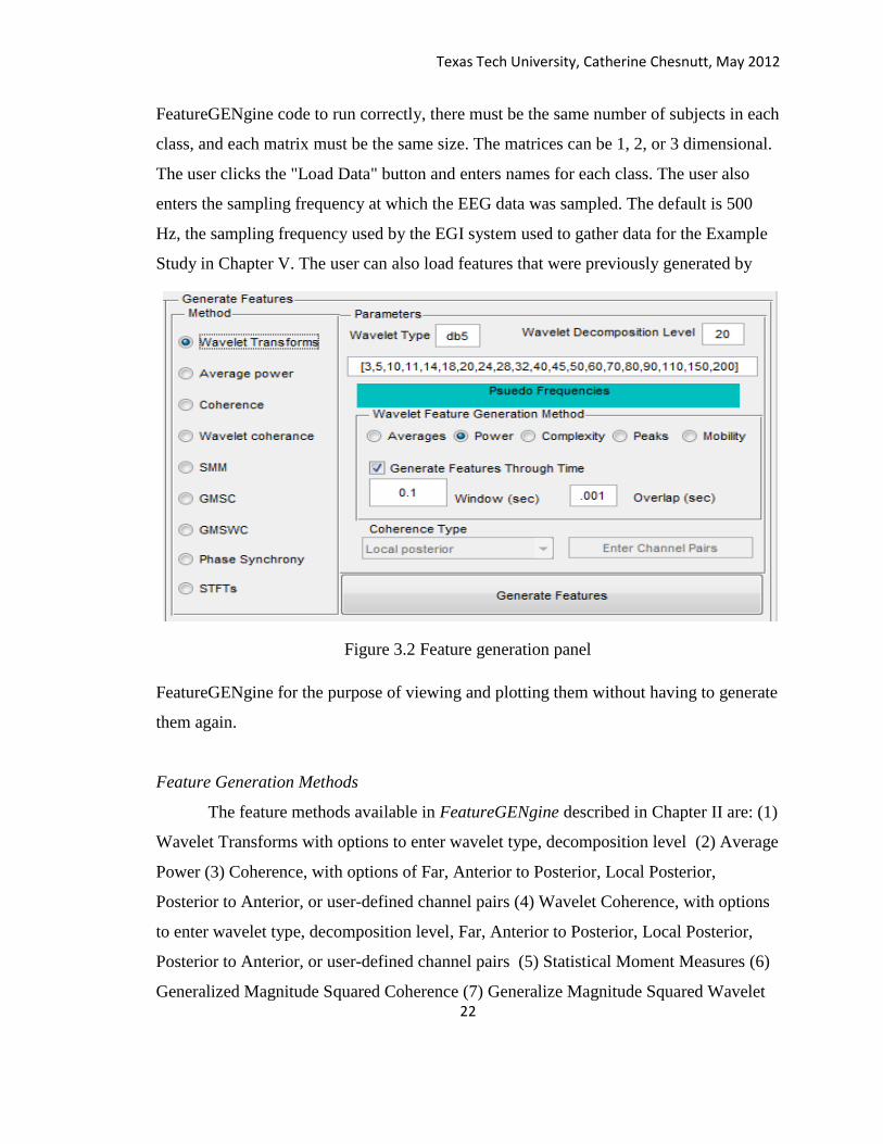
FeatureGENgine code to run correctly, there must be the same number of subjects in each

class, and each matrix must be the same size. The matrices can be 1, 2, or 3 dimensional.

The user clicks the "Load Data" button and enters names for each class. The user also

enters the sampling frequency at which the EEG data was sampled. The default is 500

Hz, the sampling frequency used by the EGI system used to gather data for the Example

Study in Chapter V. The user can also load features that were previously generated by

FeatureGENgine for the purpose of viewing and plotting them without having to generate

them again.

Feature Generation Methods

The feature methods available in FeatureGENgine described in Chapter II are: (1)

Wavelet Transforms with options to enter wavelet type, decomposition level (2) Average

Power (3) Coherence, with options of Far, Anterior to Posterior, Local Posterior,

Posterior to Anterior, or user-defined channel pairs (4) Wavelet Coherence, with options

to enter wavelet type, decomposition level, Far, Anterior to Posterior, Local Posterior,

Posterior to Anterior, or user-defined channel pairs (5) Statistical Moment Measures (6)

Generalized Magnitude Squared Coherence (7) Generalize Magnitude Squared Wavelet


23

Figure 3.3 Coherence selection

Coherence with options to enter the wavelet type and decomposition level (8) Phase

Synchrony and (9) Power Spectral Density Features.

The generations methods (1), (4), and (9) provide the options to generate five

different features: (1) Averages (2) Power, (3) Complexity, (4), Peaks, and (5) Mobility.

These methods (1), (4), and (9) have the option of generating time-segmented features

that can be plotted.

Feature Averaging, Viewing and Exporting

Due to the large amount of data that is generated when producing features and in

order to create sets of data on which to perform a t-test, the features must be averaged

Figure 3.4 Plotting feature values


24

Figure 3.5 Plotting wavelet transforms and time-segmented features

across epochs. FeatureGENgine averages the features across epochs for each subject.

Once the features are averaged, they can be viewed in the Feature Table in the GUI

window, Figure 3.4. All averaged features for each subject and for each

class can be viewed, as well as the averages across all subjects, which appears at the

bottom of the scroll list for each class.

Excel files can be created to export the features. These excel files are saved in the

current Matlab directory. One file is created per class, saving the features into sheets

labeled as the Subject Number, and the last sheet contains the features generated from

averaging across all subjects. When the "Create Excel Files" Button is pressed, the user

can rename the excel files being created, which have default names for each class based

on the class names entered when the user first loads the data.


25

Figure 3.6 Plotting wavelet transforms

Plotting Wavelet Transforms and Time-Segmented Features

Wavelet transforms, STFTs, and time-segmented features generated by methods

(1), (4) and (9) can be plotted for each class and for each channel. The plotting options

include Line, Image, and Stem Plots. An example of plotting wavelet transforms using

stem plots and image plots are shown in Figure 3.5 and Figure 3.6. The wavelet used to

calculate the CWT is plotted in the bottom right-hand corner of the panel.

Test of Significance using T-Test

Options for classifying the features from the two classes include a simple t-test

based on an alpha value. The binary matrix created by the t-test function is plotted that

highlights the features that passed the t-test. This plot opens in a new GUI window and

plots the average values of these features for each class and for each frequency band in

tables.


26

Figure 3.7 Plotting binary matrices and values of features that passed a t-test

Flexibility of FeatureGENgine

FeatureGENgine is a research tool that allows users to analyze EEG data inside

Matlab using a number of different methods. Specifically, it offers both current and new

methods of wavelet based features, and provides a way to extensively examine these

features. The program is structured in such a way as to be flexible enough to add other

functions as desired. The program's main code loads the data from arrays and stores it in

arrays within the handles structure, and performs the various functions related to the

components in the user window. The function that generates the features is separate from

the main code, and each of the feature generation methods inside this function is itself a

separate function. Other generation methods may be added by writing a new function that

handles the data in the same way as the current ones, and then by calling the new function

in the feature generation function. The main code and all the auxiliary functions it calls

are provided in the Code section.


27

Wavelet functions: stretched and compressed versions of "Mother" wavelet

EEG time domain signal convolved with wavelet

Figure 4.1 Daubechie (Db5) mother wavelet and time signal convolution

CHAPTER IV

WAVELET ANALYSIS

This chapter addresses the first two goals of this thesis. First it will be shown that

wavelet analysis is more applicable for EEG than other time-frequency analysis methods,

and some signal processing considerations of generating wavelet features will be

examined. Second, after considering currently used methods, a method of feature

generation will be described that takes advantage of the wavelet's time resolution: time-

segmented features. The choice of wavelets is examined by comparing three different

wavelets, db5, coif5, and haar, in an effort to discover which is appropriate for EEG

signals.

A Brief Overview of the Wavelet Transform

As explained in Chapter I, the wavelet transform is a newer method of time-

frequency analysis which, in contrast to Fourier analysis, provides time-dependent

frequency information of a given time signal. In Chapter I it was also shown that wavelet

transforms are a type of multi-resolution analysis that provide good resolution in the

lower frequency range, making them especially applicable for EEG signals, that have a

primary interest range of 1-100 Hz. In particular, the bands labeled Alpha (8-12 Hz) and

Beta (13-30 Hz), that describe attentive, focused thought, are of common interest. EEG


28

signals are time-dependent signals that have sudden changes in frequencies due to

changing mental processes.

A wavelet transform is calculated by taking a function, called a mother wavelet,

stretching and compressing it into different versions, and then convolving those versions

with a time signal. The wavelet transform of a signal decomposed along the

wavelet family defined by is [13]:

(4.1)

A time-signal of length will produce a number of time-domain signals, called

decompositions, each of length . The number of these decompositions equals the

number of scales, or the number of versions of the mother wavelet. Each of these

decompositions represents the original signal's correlation to that particular wavelet

throughout time. The stretched and compressed wavelets can be thought of as band-pass

filters which are applied to the signal, each having its own range of frequencies, such that

each signal it produces is limited to the range of frequencies contained in the wavelet.

Thus, a wavelet transform can be calculated on one or many scales that correspond to

decomposition levels, each having a bandwidth. Figure 4.1 repeats Figure 1.4, showing

the conceptual process of convolving a wavelet with a time signal.

The frequency and time resolution abilities of the Fourier transforms, the short-

time Fourier transform, and the wavelet transform were explained in Chapter I. This

tradeoff between time and frequency resolution in time-frequency analysis results from

the uncertainty principle. The uncertainty principle dictates that there must be a limit to

the resolution of position, and momentum :

(4.2)


29

In this equation, is equal to

, where , or

Planck's constant. In the area of special relativity, energy is related to time as position is

related to space, and the energy-time version of the uncertainty principle describes this:

(4.3)

It takes a certain amount of time to describe any amount of energy, since energy is

defined by the frequency of the state of something, whether it be a particle or a wave (or

both!). It is because of this principle that all methods of frequency or time-frequency

analysis are limited in their capabilities to provide resolution. Fourier analysis provides

all frequency, and no time resolution, Short-Time Fourier Transforms provide constant

resolution at all time and frequencies, and wavelet analysis, a type of multi-resolution

analysis, provides varying resolution across frequencies. These differences were

explained in more detail in Chapter I and are shown in Figure 1.5. Since EEG frequency

bands of interest are typically in the lower ranges, and those bands tend to be very close

together, the multi-resolution attribute of the wavelet transform makes it a good choice

for EEG signals.

Wavelet Transforms and Scales

Matlab's cwt function calculates the continuous wavelet transform of a time-

domain signal. It is called in the following way: coefs = cwt(S,scales,wavelet_type)

where S is a vector containing a time domain signal, scales is a vector containing the

levels of decomposition that the wavelet transforms are calculated upon, and the wavelet

type specifies which mother wavelet function to use. Throughout this code, the fifth

Daubechies wavelet, Db5, is used. The algorithm inside the cwt function uses the

function intwave to approximate and integrate the wavelet function. As mentioned in

Chapter II, the function is approximated using a default number of ten iterations. The

number of iterations determines the actual number of points inside this approximated

wavelet vector. Then, depending on the scale being calculated, it selects indices from the


30

approximated wavelet vector and convolves it with the time signal. It then uses the

function diff, which effectively integrates this convolution, and uses the function wkeep1

to withhold only the central part of this convolution such that the result is the same length

as the original signal.

The scales used in the FetaureGENgine code were specifically chosen to

correspond with the EEG frequency bands of interest and do not increase linearly. They

were chosen so that most of the scales would be calculated for the Delta, Theta, Alpha

and Beta bands. These scales and their corresponding frequencies are as follows:

Scales: [3,5,10,11,14,18,20,24,28,32,40,45,50,60,70,80,90,110,150,200]

Frequencies (Hz): [111.11 66.67 33.33 30.30 23.81 18.52 16.67 13.89 11.90 10.42 8.33

7.41 6.67 5.56 4.76 4.17 3.70 3.03 2.22 1.67]

The first scale, 3, corresponds to 111.11 Hz, and so forth. These vectors of scales

and their corresponding frequencies are used consistently to generate features throughout

the code, but can be changed by the user in the FeatureGENgine GUI. The scales and

their corresponding frequencies are shown for all EEG frequency bands in Table 4.1.

Table 4.1 EEG bands: corresponding scales and frequencies

EEG Frequency Band Scales Frequencies (Hz)

Delta 80,90,110,150,200 4.17, 3.70, 3.03, 2.22, 1.67

Theta 45, 50, 60, 70 7.41, 6.67, 5.56, 4.76

Alpha 28, 32, 40 11.90, 10.42, 8.33

Beta 11, 14, 18, 20, 24 30.30, 23.81, 18.52, 16.67,

13.89

Gamma 3,5,10 111.11, 66.67, 33.33

The scale of a wavelet transform does not correspond directly to a certain

frequency. Rather, these frequencies are approximations that are translated from the scale

corresponding to the maximum value of the CWT coefficients. Matlab performs this

using the function scal2freq to calculate these frequencies. To accomplish this, the


31

function scale2freq calls another function, centfrq, to calculate the center frequency by

numerically centering the wavelet and taking the maximum value of the modulus of its

Fourier spectrum. It adjusts this to different scales of the wavelet using the following

equation:

(4.4)

where is the center frequency of the spectrum of the wavelet calculated by centfrq, is

the scale of the wavelet, and is the sampling period of the data being used to calculate

the wavelet transform. Each wavelet type has different frequencies that correspond to its

scales, and some wavelets perform better than others at locating these frequencies. Thus,

some wavelets have better accuracy in representing the frequencies in the signal with

which they are convolved, depending on how well the scale of the wavelet corresponds

with the maximum value of the CWT coefficients. To explain this in greater detail,

comparisons are made between the Haar, Db5, Coif5, Gaus4, Morl, and Dmey wavelets

in the Choice of Wavelets Section of this chapter.

Wavelet Transforms and the Short-Time Fourier Transform

As mentioned previously, wavelet analysis is not the only time-frequency analysis

method used for non-stationary signals such as EEG. The Short-Time Fourier Transform

(STFT) is still used to gain time-dependent frequency information. The STFT works by

taking segments of the time-domain signal and performing a Fourier Transform on each

one. It has been used successfully in many Bio-medical applications, but has two main

limitations: (1) It is difficult to select a window length appropriate for a range of features

that vary throughout the time segments, (2) The shortening of the time-segment length to

increase time resolution will decrease frequency resolution given by [40]

(4.5)


32

where is the number of points in the time segment and is the sampling period. These

limitations make the STFT more applicable in areas where higher frequencies are of

interest and where frequency resolution is not important. Figure 4.2 (A) shows an image

and a stem plot of a spectrogram of a chirp signal ranging from 1-110 Hz that is 2

seconds long and sampled at 1000 Hz, calculated with FeatureGENgine using Matlab's

spectrogram function, which computes the STFT at a given vector of frequencies using

the Geotzel algorithm and a Hamming window [41]. Figure 4.2 (B) shows the same

signal's wavelet transform calculated with the scales corresponding to the same vector of

frequencies used in the STFT. It should be noted that the scales in Figure 4.2 (B) range

from 1 to 20, but actually correspond to the 20 scales defined above. The STFT and the

wavelet transform give similar results in Figure 4.2. As will be explained in the Time-

Segmented Wavelet Features section, generating time-segmented features based on either

the STFT or the wavelet transform requires shortening the time-segment window,

affecting the frequency resolution of both.

Wavelet Features

In general, there are two reasons to generate features from EEG data. The first is

for the purpose of classification. In this case, the features themselves, or their values, are

not examined. Using different feature extraction techniques, computer algorithms choose

the features that generate the highest classification rates. The second purpose of

generating features is to create brain models. In this case, the values of the features reveal

information about the cognitive states of the participants who were part of the EEG study,

showing not only that two brains are different, but how they are different.

A wavelet transform of a time-domain signal produces a signal of a length equal

to the original signal. A method must therefore be chosen to generate features from these

transforms. In research, these features have been generated a number of ways. One study

used energy, entropy and standard deviation of the Daubechies series (Db2 mother

wavelet) as the features generated from a five-level decomposition, and were able to

classify Epileptic EEGs at a 91.2% classification rate [23]. Another study used statistical

measures of a five-level wavelet decomposition of the data: the mean of absolute values


33

of the coefficients in each sub-band, the average power of the wavelet coefficients in

each sub-band, standard deviation of the coefficients in each sub-band, and the ratio of

the absolute mean values of adjacent sub-bands. This study found these features were

useful in classifying seizure EEGs in conjunction with a Mixture of experts (ME), a

neural network structure [24]. Although many studies use the Daubechies wavelets, one

study showed that the first of the Coiflet wavelets resulted in the most accurate

classification of EEG of both abnormal and neuro-typical signals [25]. Another study

(A) Spectrogram of chirp signal with

window size of 0.1 seconds

(B) Wavelet Transforms of chirp signal

and window size of 0.1 seconds and

overlap of 95 points

Figure 4.2 Spectrogram and wavelet transform of chirp signal of 1-110 Hz


34

examining EEG artifacts generated wavelet features using the power spectrum, variance

and mean of the Haar mother wavelet [26]. Another study used an Amplitude

Modulation method to extract features from the wavelet decompositions of EEG data,

that defines changes in the time-signal's envelope at its sampling frequency, and produces

high classification rates using SVM neural networks [42].

These studies generated wavelet features of different methods with the purpose of

producing improved classification rates between groups using different algorithms. Some

of these algorithms involve data reduction techniques to extract features that produce the

highest classification rates. While high classification rates are beneficial in algorithms

that attempt to separate EEG data into groups, it can sometimes be difficult to interpret

physical meaning from these features, for the purposes of understanding neural processes

within the brain. Classifying EEG data is useful, but when there is a need to create brain

models to understand the processes of the brain, such as with autistic subjects, the

physical meaning behind the features must be retained. One study separates the WT into

segments to find an optimal active time segment and then extracted fractal feature vectors

for a classification using a linear classifier [45], which does make use of the WT's time

resolution, but is for classification purposes, not brain models. Many times, the feature

extraction and data reduction techniques remove this attribute of the data, especially

where nonlinear transformations are involved. For EEG data to remain physically

interpretable, it is helpful to stay close to the established meaning of power in the five

EEG frequency bands introduced in Chapter II: Delta, Theta, Alpha, Beta, and Gamma,

all corresponding to different general cognitive states. To accomplish this, time-

segmented wavelet features are generated based on the wavelet power in the EEG bands.

Time-Segmented Wavelet Features

The current methods mentioned above, while using wavelet transforms to

generate features, are generating one value or feature per transform. This inevitably

averages out the time-dependent information. Regardless of which method of generation

described thus far is used on the wavelet transforms, although they might describe the

shape or overall nature of the time-domain signal, the temporal information is still


35

averaged out. Being able only to describe the shape of the signal, such as several of the

aforementioned studies did by using means and standard deviations of the transforms,

provide an ambiguous interpretation of the physical meaning of the data, with the

possible exception of string length (Complexity) being linked to intelligence. A possible

solution to this is to generate these features in segments of time, in a manner similar to

the STFT. To create these time-segmented features, FeatureGENgine first computes the

wavelet transforms as it normally would using Matlab's cwt function. The user specifies a

window size for the features such that each wavelet transform, a function of time itself, is

divided into n of these segments. Features are then generated on each one of these n

segments. This produces one feature per time segment per scale of decomposition, per

channel, per epoch. EEG data epochs can range from seconds to minutes. This makes the

amount of data generated by these time-segmented features quite large. In the case of the

example study, 64 channels, 15 epochs of length 1.4 seconds, a sampling rate of 500 Hz,

a window size of 0.1 seconds, and a wavelet decomposition of 20 scales produces an

entire feature matrix of size 20x14x15x64. One of these is calculated per subject. In our

example study there are two classes, each containing five subjects. The computational

time required for time-segmented wavelet power features is 153.14 seconds per subject.

The time required to calculate time-segmented features from the STFT of all the data per

subject is 24.35 seconds.

The time segment window size of the time-segmented wavelet transforms

determines the frequency resolution of the features. If the window size is too large, the

features generated at the smaller scales, or higher frequencies, are almost undetected.

This shows the ineffectiveness of generating features based on the entire wavelet

transform (a very large window) without breaking it up into segments; the temporal

information is simply averaged out. Basically, it is using a function specifically to

produce some information and then discarding that information. To demonstrate the

importance of the window size, wavelet power features of 20 decomposition levels are

generated from a chirp signal ranging from 1-110 Hz that is 2 seconds long and sampled

at 1000 Hz. Figure 4.3 shows a stem plot of the features computed with a 0.01 second

window (200 time blocks) and a 0.001 second window (2000 time blocks).The smaller


36

wavelet scales should be able to reveal the higher frequencies of the signal. The smaller

window size of 0.001 makes the number of features equal to the original length of the

signal, 2000, and should therefore be able to show the entire frequency range of the

signal, which it does in the red portion of the time axis. The plot (A) with the larger

window, however, does not show the higher frequencies located toward the end of the

chirp signal. It should be noted that the scales shown in Figure 4.3 correspond to the

(A) STFT of chirp signal with


(B) Wavelet features of chirp signal with


Figure 4.3 Time-segmented wavelet power features using different widow sizes


37

vector of 20 scales defined earlier, and are labeled as being from 1 to 20 in an effort to

make the plots clearer.

In contrast, when the same window size is used in the STFT to generate features,

the decrease in frequency resolution in these lower frequencies is clear in Figure 4.3 (A)

and (B). Both the time-segmented wavelet features and the STFTs were calculated with

the same window size of 0.01 seconds. The decrease in frequency resolution due to Eq.

4.2 is evident in the STFTs, while the wavelet transforms retain their lower frequency

resolution.

Note the purpose of examining the method that retains the greatest amount of time-based

frequency information when generating features from wavelet transforms and STFTs.

Whether taking wavelet transforms or STFTs of EEG data, a large amount of data is

produced. We need to produce characteristic features of this data that will help us identify

two groups as different, and be able to interpret those characteristics in a physically

meaningful way. Since there has been well-established physical meaning in the various

EEG frequency bands we have described, the goal is to retain as much information about

these bands as possible. It is clear that wavelet transforms, although less computationally

efficient in this implementation, are able to generate more features of the original signal.

Windowing the Time-Segmented Wavelet Features

Windowing is an essential part of analyzing signals. It is necessary to truncate a

segment of an aperiodic time signal, such as EEG, for representation in a computer, since

an infinite time signal like this is larger than the computer's memory storage [40]. The

type of window used can affect the resulting frequency spectrum, since the windows

themselves contain their own frequency content. In using the blocproc function to

generate time-segmented features of the wavelet transforms, segments are cut out of the

time-signal (wavelet transform), effectively applying a rectangular window. The resulting

features contain information about the rectangle's frequencies as well as the original

signal. In order to minimize these effects, a Hamming window function is multiplied with

the wavelet transforms before they are processed inside the blocproc function. An overlap

value may also be specified.


38

Wavelet Test Data

The Db5 wavelet was scaled to all of the 20 scales defined above and used as

input signals. The transform, computed on the same 20 scales, is shown in Figure 4.4 for

the first and last scales, 3 and 200, corresponding to 111.11 Hz and 1.67 Hz, respectively.

It is interesting to note that while the highest scale in (B) (lowest frequency) was not at

all detected on the lower scaled wavelet transforms, the lowest scale (A) wavelet signal

(highest frequency) was still detected on the highest scaled (lowest frequency) transform.

This is due to the fact that the continuous wavelet transform contains overlap between

scales.

Choice of Wavelets: Harmonics and Frequency Detection

One study found that the Coif wavelet family produced high classification rates

for EEG data [25]. When testing a 2-second chirp signal of 1-110 Hz with the Haar, Db5,

Coif5, Gaus4, Morl, and Dmey wavelets, the coif5 shows the least amount of harmonic

interference, shown in Figure 4.5. This lack of interference is a possible explanation for

the study's findings. The reason for the harmonic interference is due to the frequency

spectra of the wavelets, shown in Figure 4.7 for the Haar, Db5, Coif5, and Dmey

wavelets. Of these four, the frequency spectrum of the Coif5 wavelet shows the least

amount of harmonic frequencies.

The frequency corresponding to a certain scale of a wavelet transform is based on

its center frequency - the maximum of the modulus, or absolute value of its Fourier

spectrum after it is numerically centered. Each type of wavelet has different frequencies

that correspond to its scales, and some wavelets perform better in detecting the

frequencies of the signal with which they are convolved. In using wavelets to generate

EEG features, it is very important that the wavelet perform well. One of the main

objectives in this thesis is to create time-segmented wavelet features that have a physical

meaning in order to develop models of the brain. This physical meaning is attached to the

EEG frequency bands, so that the wavelet used must have its scales match up well with

the frequencies they represent. If they do not match up well, there is less certainty that


39

Figure 4.4 Wavelet transforms of Db5 wavelet signals

the wavelet power features generated represent the correct frequency bands. For instance,

some features found to be significant (with a t-test or other test of significance) in the

Alpha band might actually have been in one of the bands beneath or above it, in the Theta

or Beta bands. In order to test the performance of different wavelets in detecting these

frequencies, Matlab's scalogram function is used with wavelet coefficients generated

from a plain 14 Hz sine wave of 1 second [43]. To be more precise, a wavelet transform

is calculated for a 14 Hz sine wave and the energy of each wavelet coefficient is plotted.

The maximum of these energy coefficients should correspond to the scale calculated by

scal2frq using 14 Hz as the input frequency. This is done for six different wavelets in

Figures 4.6. For each plot, the horizontal red line represents the scale at which the

wavelet corresponds to 14 Hz, the frequency of the input signal, according to the scal2frq

function. The location of the red line with respect to the maximum energy of the

coefficients and the amount of variation of the energy across scales describes the

performance of the wavelet in locating the 14 Hz frequency. The scales corresponding to

the Haar, Db5, Coif5, Gaus4, Morl, and Dmey wavelets are 71, 48, 49, 36, 58, 47,

respectively.

(A) Wavelet Transforms of Wavelet of

Scale 3

(B) Wavelet Transforms of Wavelet of

Scale 200


40

Figure 4.5 Wavelets of Haar, Db5, Coif5, Gaus4, Morl, and Dmey tested

with chirp signal


41

Of the six wavelets examined, the Morl and Gaus4 appear to have the best

frequency detection. The red horizontal line representing the scale that corresponds to 14

Hz travels very nearly across the center of the maximum of the energy coefficients, and

these coefficents do not vary quite so much across the scales. While the Coif5 wavelet

shows little harmonic interference in its representation of the chirp signal, its scalogram

shows its frequency detection as less than perfect. While the Morl wavelet does show

Figure 4.6 Scalograms of Haar, Db5, Coif5, Gaus4, Morl, and Dmey wavelet coefficients

of 14 Hz sine wave (scale corresponding to 14 Hz represented by red horizontal line)


42

some interference in its representation of the chirp signal, it provides good frequency

detection.

Figure 4.7 - Frequency Spectra of Haar, Db5, Coif5, and Dmey wavelets

Types of Wavelet Features

Averages

Taking averages of wavelet transforms might defeat the purpose of using them.

The appeal of a wavelet transform is its ability to retain temporal information, so

averaging the various decomposition levels practically erases this information. Still,

taking averages of the wavelet transforms has yielded features which have passed a

significance test.


43

Power

Calculating the average power of the wavelet transforms yields more significant

features in the sample data than averaging the entire wavelet transform. It is similar to

calculating regular power in designated frequency bands, except that instead of having

the five bands of Delta, Theta, Alpha, Beta and Gamma, there are as many bands as there

are decomposition levels, since each decomposition is effectively a band pass filter of the

time-signal. These average power features have a meaning similar to conventional

average power in the EEG bands, only they have higher frequency resolution. This makes

it easier to divide the EEG bands into sub-bands which also have meaning according to

research: low-Beta, high-Beta, etc.

Complexity and Mobility

Using complexity and mobility to calculate wavelet features has yielded many

significant features in the sample data, particularly complexity. When complexity is used

on test data that contains wavelets as input signals, the features are clearly different for

each decomposition level. They increase from very small to very large values from the

lower to the higher scales, respectively.

Peaks

Features can be generated by calculating the number of peaks in the wavelet

transform that cross a certain threshold. The FeatureGENgine code uses a threshold of

90% or 0.9 times the highest point in the signal.

Conclusions

To generate wavelet features in a fashion that retains the physical meaning of the

features, wavelet power features are generated in segments of time. The response of the

STFT and the wavelet transform to the windowing required for generating time-

segmented features makes the wavelet transform more appropriate, since it provides more

frequency resolution in the EEG ranges of interest. The choice of mother wavelet used to


44

generate these features should reflect the wavelet's level of harmonic interference and its

ability to detect frequencies that align with its scales. The Coif5 wavelet provides good

frequency detection while having little harmonic interference. Results from using wavelet

power features and time-segmented wavelet power features are compared with an

example EEG study in the next chapter.


45

CHAPTER V

EXAMPLE STUDY: ATTENTION NETWORKS OF AUTISTIC INDIVIDUALS

Participants were recruited for a study that examined the differences in attention

between neuro-typical children and those diagnosed with Autism Spectrum Disorder

(ASD). The goal of the study was to inspect the differences in areas and activations of

the brain that occur as a result of a mental task involving a 'distracting' stimulus. It is

thought that individuals with ASD have a tendency to hyper-focus on aspects of their

environment, to their detriment.

Background

Attention refers to the cognitive process of focusing on a certain aspect of one's

environment while ignoring other aspects of it. Cognitive psychology suggests that there

are several types of attention. In particular, selective attention is a type of executive

control, and describes the extent to which the other aspects of an environment are

ignored. A study in 2005 established a technique to assess selective attention, called the

Attentional Network Task (ANT) [47]. The task involves two different stimuli. The first

is a picture of five fish that all face the same direction (congruent), and the second is the

same set of fish with the middle one facing the opposite direction from the others

(incongruent). The study discovered an association between selective attention and

activation in the anterior cingulate and frontal cortex. There is an abnormality in the

selective attention processes of autistic individuals when compared with neuro-typical;

autistics tend to hyper-focus on a specific aspect of their environment, and sometimes

those aspects are irrelevent. The study in this chapter was conducted to examine whether

the activation regions for each type of ANT stimulus were different for autistic and

neuro-typical subjects. It is thought that when presented with the ANT stimuli, autistic

individuals process both congruent and incongruent types of stimuli in a similar manner,

while neuro-typical individuals process the two differently. The neuro-typical brain

should be more distracted by the presence of opposite-facing fish in the incongruent

stimulus, while the autistic brain fails to process the surrounding fish. Thus, the


46

hypothesis for this study is that there will be a large number of differences between

autistic and neuro-typical brain patterns in response to the incongruent fish, more

differences within the autistic group than neuro-typical between types of stimuli, and that

these differences will occur in the area linked to selective attention: the prefrontal cortex

and the anterior cingulate.

Stimulus Materials and Procedure

Each participant was given a handedness questionnaire upon arriving at the

location of the study. The study was then explained to them briefly and they were shown

examples of the stimuli they would be seeing on the computer screen during the EEG

recording. After these instructions were given, head measurements were made and an

EGI 64-Channel EEG net was placed on their heads after the proper preparation of the

net. The participant was then placed in a sound-proof room with or without his or her

legal guardian and performed the test on the computer screen.

Subjects

Participants were between the ages of 13 and 18. Those in the ASD group had

been previously diagnosed with a form of ASD. Those in the controls group were

selected from a typically developing individuals of the same age group.


47

Attention Test

The test itself consists of a series of pictures of fish in the middle of the screen. In

each picture, the middle fish is facing either the same direction or the opposite direction

of the fish on either side of it, show in Fig.5.1. Figure 5.1 (A) shows a congruent trial, all

the fish are facing the same direction. Figure 5.1 (B) shows an incongruent trial, the

middle fish is facing opposite to the ones on its left and right. Each trial presented to a

subject contains either a picture of congruent-facing fish or incongruent-facing fish. The

subject then pressed a button to signify which direction the middle fish was facing.

assumed that the cognitive responses that distinguish between groups occurs primarily in

this initial time period.

The purpose of the study was to identify neuronal differences in the attentional

networks of neurotypical children and those diagnosed with Autism Spectrum Disorder.

These differences are possibly due to the ASD child's tendency to hyper-focus, meaning

they are less affected by the opposite-facing directions of the surrounding fish than a

neurotypical child would be.

Recording and Preprocessing EEG Data

Exporting

The EEG data were recorded using EGI's Net-Station software and a 64-Channel

net. The test was created in E-prime, which is configured to communicate with EGI

during recording. The EEG files were filtered with a 60 Hz notch filter, a 0.1 Hz low pass

filter, and re-montaged to a 10-10 montage format before exporting from Net-Station.

They were then imported into EEGLab. The data segments removed included data

recorded between stimulus trials and before and after the trials begin and end.

Independent Component Analysis

Independent Component Analysis (ICA) is a standard technique for removing

artifacts from EEG data. It isolates components that are embedded within the data so that

they can be removed. Components due to heart rate, eye-blinks, and muscle movement


48

Figure 5.2 Scalp maps of ICA components using EEGLab

can be detected by ICA. EEGLab offers an ICA tool to remove such artifacts. To remove

eye-blink artifacts, ICA was performed on the data in EEGLab. These are chosen at the

discretion of the user, but are usually identifiable and are described in the EEGLab

manual [27]. The criteria for recognizing eye blinks, described in the EEGLab manual

and applied to this data are the following: (1) The smoothly decreasing EEG spectrum

(2) The scalp map shows a strong far-frontal projection (3) It is possible to see individual

eye movements in the component activity graph [28]. Likewise, the criteria for

determining relevant brain artifacts that should remain in the data are: (1) Dipole-like

scalp maps (2) Spectral peaks at typical EEG frequencies (i.e., 'EEG-like' spectra) (3)

Regular ERP-image plots (meaning that the component does not account for activity

occurring in only a few trials). There are two ICA algorithms available in EEGLab: one

calls the runica.m file and one calls the jader.m file. The runica algorithm is

recommended in the manual and was used in this instance. According to the manual, any

physiological significance to the results of using these different algorithms has not been

determined. They return nearly equivalent results when used with low dimensional data


49

which fulfill the assumptions of the algorithm [29]. The runica algorithm is proposed to

be suitable for EEG data and is an implementation of the ICA algorithm written by Bell

and Sejnowski in 1995 [30]. It is thought to be suitable because the nature of the spatial

ambiguity of the EEG data, which the algorithm is able to take into account as it

separates source identification from source localization using blind source separation

[31]. Figure 5.2 shows the first twelve ICA component scalp maps for a typical EEG

scan. The first and second components, shown by the arrows, most likely contain eye-

blink artifacts. Components like these are removed in the example study.

Epoching

The data are then segmented into epochs using EEGLab. The parameters for the

epochs begin with the stimulus flag (the point at which the participant is shown the

pictures of the fish) and end 1.4 seconds after the stimulus flag. The sampling rate is 500

Hz, making each epoch 700 data points long. The time length of the epoch was chosen

according to the average response time, that occurred within 1.4 milliseconds.

Exporting to Matlab

The files were then exported from EEGLab into .mat files. Each dataset in

EEGLab contains a structure with information fields. The data field contains the

processed data. Each data field of each dataset that is part of the study is then called in

the matlab command line and placed in an array using the following command:

EEG_array_1{i} = ALLEEG(i).data

Two separate arrays are made, one for each class of data. For each class, i represents the

index of the subject. For a class with five subjects, i ranges from 1 to 5. These two arrays

are then saved into a .mat file with the following command:

save EEG_arrays EEG_array_1 EEG_array_2


50

This saves EEG_array_1 and EEG_array_2 into EEG_arrays.mat, a file which appears in

the current Matlab directory folder.

Results

A t-test is a test of significance designed to show whether two groups of data are

statistically significantly different. The t-test used in FeatureGENgine is a two-tailed test,

meaning that it tests the null hypothesis against the alternative that the means of the two

groups are different. A t-test is a simple way to tell whether the features generated are

able to distinguish the two groups of EEG data. Not only is it important to see whether

these features from the two groups are significantly different, but it is also of great

interest to examine the values of those features. The values have physically meaningful

interpretations. The results of the t-tests performed on the time-segmented features can be

viewed as a binary matrix. Since each t-test returns either a one (for passing) or a zero

(not passing), a matrix of ones and zeros of size Channel x Time Segments, or 64x14, is

produced for each scale. The FeatureGENgine GUI plots these matrices as images

according to each scale or corresponding frequency, such that ones are represented with a

white square and zeros remain black. It also plots an overlay of all the binary matrices

that fall under a specific EEG bandwidth. Since more than one feature can pass the t-test

in the same time-segment (there are multiple scales per band), these overlaid images are

gray-scaled. The highest number of features that passed are represented by the whitest

square, while the lowest number that passed for a time-segment, which would be one, are

represented by a darker shade of gray. These matrices illustrate the advantage of using

time-segmented wavelet features. Some features that pass the t-test are localized in time

segments. Physically, this means that significantly different activity between groups

occurred at specific times. Also, some of the features which passed the t-test have higher

or lower average values between groups in certain time segments, while different

features which passed at a different place in time have opposite average values between

groups. This will become apparent in the first results category, ASD Congruent vs. ASD

Incongruent.


51

The binary matrices produced by the features passing the t-test at alpha = 0.05 are

shown for each of the four categories: ASD Congruent vs. ASD Incongruent, ASD

Incongruent vs. Controls Incongruent, Controls Congruent vs. Controls Incongruent, and

ASD Congruent vs. Controls Congruent. It is not only of interest to find distinctions

between ASD and neuro-typical subjects, but also to find differences within the ASD and

Control groups.

A table showing the channels, frequency, and number of features that passed the

t-test is given for each category and for each type of feature. The actual values for

average power and wavelet power are listed, and the tables with the time-segmented

wavelet features show only the features that passed in the Alpha and Beta bands and

whether the average value for a feature that passed the t-test was higher in the first group

or the second group.

ASD Congruent vs. ASD Incongruent

There were no features that passed the t-test for conventional average power

between the ASD congruent and ASD incongruent classes. For time-averaged wavelet

power features, 6 features passed the t-test, shown in Table 5.1. For time-segmented

wavelet power features, 91 features passed the t-test. The channels and time locations of

those which passed in the alpha and beta bands and for all bands are shown in Figures 5.3

and 5.4, respectively. The details of these features are given in Table 5.2. Note that of all

the significant channels in time-averaged wavelet power features, the same channels

arose in the time-segmented wavelet features except for Channel 9 (F1) and 48 (TP8),

although Channels similar to these, F10 and T10, did pass.


52

Figure 5.3 Time-segmented wavelet power features that pass the t-

test in Alpha and Beta bands for ASD congruent vs. ASD

incongruent

Figure 5.4 Time-segmented wavelet power features that pass the t-

test in all bands between ASD congruent and ASD incongruent

Table 5.1 - Time-Averaged Wavelet Power Features

Frequency

Band

Channel Class 1 Average Class 2 Average

Delta 1 - F10 125.8844

84.8390

Theta 48- TP8 4.8296

6.3251

Alpha 48-TP8 3.7821

5.0799

Beta 0 0 0

Gamma 9 -F1, 52-T8, 55-T10 0.0202

0.0143


53

Table 5.2 Time-segmented wavelet power features for ASD congruent vs. ASD

incongruent

Frequency Total

Number

of

Features

Channels and

Segment

Locations ( ) of

Total Features

Number of

Features

With Larger

Average

Value

Channels

of Higher

Features

Class

Alpha 8.33 6 AF3(3), F3(3),

P1(4), P2(3),

T8(10), FT8(7)

5 AF3, F3,

P2, T8,

FT8

2

10.42 7 AF3(3), P5(4),

P3(4), P7(6),

P1(4), P9(6),

PO3(1)

6 P5, P3,

P7, P1,

P9, PO3

1

11.90 5 P7(6), P1(4),

P9(6), PO3(1),

FC2(9)

4 P7, P1,

P9, PO3

1

Beta 13.89 3 P7(6), PO3(1),

FC2(9)

2 P7, PO3 1

16.67 2 Fz(3), PO3(1) 1 PO3 1

18.52 1 Fz(3) 1 Fz 2

23.81 1 AFz(5) 1 AFz 2

30.33 3 Fz(10) AFz(5),

C2(10)

3 Fz, AFz,

C2

2

As an example of how to interpret the data in Table 5.2, six total features passed

the t-test using time-segmented wavelet features with a frequency of 8.33 Hz. The

channels that contained these features were AF3, F3, P1, P2, T8, and FT8, and the time

segments in which they passed were 3, 3, 4, 3, 10, and 7, respectively. Five of these

features had higher average values in Class 2, the trials corresponding to the incongruent

stimulus.


54

(A) Time-segmented wavelet power features of 3.70 Hz (Delta Band)

(B) Time-segmented wavelet power features of the Beta band

Figure 5.5 Time-segmented wavelet features between ASD congruent

and ASD incongruent

An interesting part of the results for this group was made visible only by both the

time resolution and the superior low-frequency resolution provided by the wavelet

features. For many of the frequencies listed in Table 5.1, the number of higher features

would show up time segments located in the middle of the epoch, and then switch in the

later time segments toward the end. For instance, for the 3.70 Hz features, six out of ten

features were higher in Class 1, but all of those features were located in the same time

segment, which was near the end at 1.2 seconds. The other four features, which were

higher in Class 2, were located clustered together over two time segments in the center of

the epoch. This is shown in Figure 5.5 (A) for 3.70 Hz, where all of the features in time

segment number 12, or 1.2 seconds, were higher in Class 1, Congruent, and the three

features in the middle in segments 6, 7, and 10 were higher in Class 2. Similarly, in the

Beta band in Figure 5.5 (B), 3 out of the 10 features which passed were higher in Class 1,


55

and all 3 of these segments were located toward the beginning of the epoch, at segments

1 and 6. The rest of the features at segments 3, 5, 9, and 10 were higher in Class 2. These

discrepancies between features across time may provide an explanation as to the

differences between time-averaged wavelet power features and time-segmented ones.

There are some time-segmented features which reflect the time-averaged features

throughout all bands, and some that do not agree with them, depending on the time

segments in which they are located. This shows that time-segmented features may reveal

a much more dynamic picture of brain activity.

Features that passed the t-test at alpha = 0.05 were found using Far and Local

Posterior frequency coherence.

Table 5.3 Far coherence between ASD congruent and ASD incongruent trials

Table 5.4 Local Posterior coherence between ASD congruent and incongruent trials

Similar channels passed the significance test for the same coherence categories as

in the regular coherence features, Far and Local Posterior, but many of them passed in

different bands, shown in Tables 5.5 and 5.6. The O1-F7 channel pair passed for both the

frequency and the wavelet coherence types, but in the Theta band for the frequency

coherence and in the Delta band for wavelet coherence. For both types however, the

average was higher in Class 2, incongruent trials.

Channel Pair Frequency Band Class 1 Average Class 2 Average

O1-F7

Theta 0.180217 0.212842

P4-F4

Delta 0.263669

0.211623


O2-C4

Delta 0.248966 0.18383

Gamma 0.242735

0.216649


56

Table 5.5 Far wavelet coherence between ASD congruent and ASD incongruent trials

Table 5.6 Local posterior wavelet coherence between ASD congruent and

ASD incongruent trials

Controls Congruent vs. Controls Incongruent

In the comparison between controls congruent trials and controls incongruent

trials, no features passed the t-test for average power, 2 features passed for time-averaged

wavelet power, and 54 features passed the t-test for the time-segmented wavelet features,

shown in Tables 5.7 and 5.8. There were no features that passed the t-test for either

frequency coherence or wavelet coherence. Figure 5.6 shows the features for the Alpha

and Beta bands, and Figure 5.7 shows all of the features that passed the t-test (in all

bands). Overall, in this category, most of the significant features were higher in the ASD

congruent group. However, the time features reveal some important differences. In the

Delta band, many of the significant features are higher in the controls congruent class in

the early time segments, and are higher for other features in the controls incongruent

class in the later time segments.


P4-F8 23.81(Beta) 3.5551 2.6035

30.30 Hz (Beta) 3.2774 2.4946

O1-F7 1.67 (Delta) 9.2611 11.868

P8-F8 30.30 Hz (Beta) 3.0060 2.4097


P8-C4 Gamma 3.2025 3.8487

O2-C4 Gamma 6.9675 5.3305


57

Table 5.7 Time-averaged wavelet power features between controls congruent and

controls incongruent

Table 5.8 Time-segmented wavelet power features between controls congruent

and controls incongruent

Frequency Band Channel Class 1 Average Class 2 Average

Gamma

TP10 0.1354 0.1140

CP1 0.0170 0.0120

Frequency Total

Number

of

Features

Channels

and Segment

Locations( )

of Total

Features

Number

of

Features

With

Larger

Average

Value

Channels of

Higher

Features

Class

Alpha 8.33 4 Fz(4), F1(8),

AF3(8), F3(8)

4 Fz, F1, AF3,

F3

1

10.42 6 F1(5,8),

AF3(5,8),

PO4(7), P6(5)

5 F1,AF3, P6 1

11.90 3 F1(5),

AF3(5),F3(5)

3 F1, AF3, F3 1

Beta 16.67 1 61(9) 1 61 2

18.52 2 T10(9), 61(9) 2 T10, 61 2

23.81 3 F7(6),

CP1(6), 61(9)

3 F7, CP1, 61 2

30.33 4 AF3(1),

F9(6),

CP1(4),

T10(9)

2 F9, T10 2


58

Figure 5.6 Time-segmented wavelet power features that pass the t-test in Alpha and Beta

bands between controls congruent and controls incongruent

Time Segments (seconds)

Figure 5.7 Time-segmented wavelet power features that pass the t-test in all bands between

controls congruent and controls incongruent



59

ASD Congruent vs. Controls Congruent

For the comparison between ASD congruent and controls congruent, one feature

passed for average power, 7 features passed for plain wavelet power, and 278 features

passed for time-segmented wavelet power features, shown in Tables 5.9, 5.10 and 5.11,

respectively. The two channels with the most time-segmented wavelet features that

passed were 23 and 17, or T9 and F9. Some significant features were higher for one class

in during certain segments, and other features are higher for the other class at other

segments. The time-segmented wavelet power features are shown in Figures 5.8 and 5.9

for Alpha and Beta bands and for all bands, respectively.

Table 5.9 Average power features between ASD congruent and controls congruent

Table 5.10 Time-averaged wavelet power features between ASD congruent and controls

congruent

Frequency

Band


Gamma O1 3.5178

1.9923

Frequency

Band


Theta TP8 - 48 6.3251 4.2719

Alpha 61 6.9294 4.5638

Gamma CP1 - 21 0.0130 0.0160

P7 - 30 0.1787 0.0945

F6 - 59 0.0779 0.1031

61 0.1434 0.1048

O1 - 35 0.9332 0.6816


60

Figure 5.9 Time-segmented wavelet power features that pass the t-test in all bands

between ASD congruent and controls congruent

Time Segments

(seconds)

Figure 5.8 Time-segmented wavelet power features that pass the t-test in Alpha and

Beta bands between ASD congruent and controls congruent



61

Table 5.11 Time-segmented wavelet power features between ASD congruent and

controls congruent

Frequency Total

Number

of

Features

Channels and

Segment

Locations( ) of

Total Features

Number of

Features

With

Larger

Average

Value

Channels

of Higher

Features

Class

Alpha 8.33 14 F2(20), FC1(1),

F9(11),F7(4),

C3(6,11),

T9(11), P1(3,4),

Poz(11),

PO4(11), O2(5),

CP2(13), 62(3)

6 FC1, F9,

F7,C3,T9,

CP2

1

10.42 8 F2(7),

CP1(7),T9(4),

P1(4), Pz(3),

Poz(3), O2(5),

P2(4)

5 P1, Pz,

Poz, O2,

P2

2

11.90 6 F2(7), F9(12),

T9(4), P1(4),

Pz(3), Poz(3),

3 P1, Pz,

Poz,

2

Beta 13.89 12 FC1(2), FC3(2),

C1(2), F9(12),

F7(4), T9(4,10),

P1(4),

T10(5,10),

61(5,10)

8 FC1, FC3,

C1, F9,

F7,T9,

T10(10),

61(10)

1

16.67 17 F10(10), Fz(7),

FC1(2), F1(7),

AF3(7), C1(2),

F7(9),CP1(7),

T9(4,9,10),

T10(8,10),

61(5,8,10),

64(10)

17 F10,

Fz,FC1,

F1, AF3,

C1, F7,

CP1,

T9,T10,

61, 64

1


62

ASD Incongruent vs. Controls Incongruent

There were 7 features that passed the t-test for average power,19 for time-

averaged wavelet power, and 324 for time-segmented wavelet power features. The values

of these features are given in Tables 5.12, 5.13, and 5.14. The locations of the features in

the Alpha and Beta bands are shown in Figure 5.10 and in the head diagrams in Figure

5.11.

Table 5.12 Average power features between ASD incongruent and controls incongruent

18.52 17 FC1(2), F1(9),

FP1(7), AF3(9),

F9(9), F7(6,9),

C3(8),

CP1(7,8), T9(4,

10), T10(8, 10),

61(8,10), 64(10)

14 FC1, F1,

FP1, AF3,

F9, F7,

C3, CP1,

T9, T10,

1

23.81 15 Fz(8), Afz(8),

F1(8),FP1(6,8),

F5(6), F9(6),

F7(6), FT7(6),

C3(5),

CP1(6,7,8),

T9(6,10)

15 Fz, Afz,

F1, FP1,

F5, F9,

F7,FT7,

C3, CP1,

T9

1

30.33 18 Fz(8), Afz(8),

F1(8), FP1(6),

F9(6), FT7(6),

C3(5), CP1(7),

T9(3,6), P7(12),

Pz(2), CP2(4,6),

P4(8), CP6(6),

C2(12),

FC2(12),

17 Fz, Afz,

F1, FP1,

F9, FT7,

C3, CP1,

T9, P7,

CP2, P4,

CP6, C2,

FC2

1

Frequency

Band

Channel Class 1

Average

Class 2 Average

Delta F9 - 17 11.5974 8.9519

Alpha F9 - 17 6.3426 4.9994

Theta T9 - 23 3.6662 2.5049

Beta T9 - 23 2.9457 1.9083


63

Table 5.13 Time-averaged wavelet power features between ASD incongruent and

controls incongruent

Table 5.14 Time-segmented wavelet power features between ASD incongruent and

controls incongruent in Alpha and Beta bands

Frequency

Band

Channel Class 1

Average

Class 2 Average

Alpha T9 - 23 4.9183

3.0949

T9 - 23 6.6380

4.0178

F9 - 17 7.4275

5.1098

Beta T9 - 23 1.1681 0.7002

T9 - 23 2.0770 1.1193

Cp6 - 46 1.6013 1.1448

Frequency Total

Number

of

Features

Channels

and

Segment

Locations ( )

of Total

Features

Number of

Features

With

Larger

Average

Value

Channels

of Higher

Features

Class

Alpha 8.33 19 F10 (3),

AF4(4),

FP2(4),

AF3(8),

F3(1), F9(7),

F9(11),

F7(9),

T9(2,11),

P7(1),

Poz(3),

P2(3),

CP2(11),

TP10(13),

T10(11),

16 AF4, FP2,

AF3, F3,

F9, F7,

T9,P7,

CP2,

TP10,

T10, F4,

64

1


64

F4(4), 64(7,

11)

10.42 19 F2(9),

FP2(9),

Fz(9),

AFz(9),

F1(8),

FP1(5,8),

AF3(5,8),

F3(8), C1(9),

F9(5,7),

PO3(1),

Pz(3),

Poz(3),

PO4(3),

CP6(5),

F4(9), 63(5)

16 F2, FP2,

Fz, F1,

FP1, AF3,

F3, C1,

F9, PO3,

CP6, F4,

63

1

11.90 12 FC1(8),

Afz(9),

F1(5,8),

FP1(8),

AF3(5,8),

F9(5),

C3(7,14),

PO3(1),

TP10(13),

12 FC1, AFz,

F1, FP1,

AF3, F9,

C3, PO3,

TP10

1

Beta 13.89 10 FP2(2),

FC1(8),

FP1(8),

AF3(5),

F9(1,5,12),

F7(5),

C3(14),

CP2(2),

10

FP2, FC1,

FP1, AF3,

F9, F7,

C3, CP2

1

16.67 11 Fz(13),

Afz(13),

FP1(13),

F9(1, 12),

C3(14),

T9(7),

CP2(1,2),

T10(14),

63(5)

11 Fz, Afz,

FP1, F9,

C3, T9,

CP2, T10,

63

1

18.52 14 Afz(13), 14 Afz, F1, 1

Table 5.14 Continued


65

Conclusions

Results

The study was conducted with the hypothesis that there would be a large number

of differences between the autistic and neuro-typical (control) groups when examining

brain responses to the incongruent fish, reflecting the selective attention abnormality

present in autism and that there would be a more differences within the autistic group

than within controls between the two types of stimuli. It was also hypothesized that these

differences would occur in an area associated with selective attention: the prefrontal

cortex and anterior cingulate. As postulated, the largest number of features that passed a

F1(13),

FP1(13),

AF3(13),

F9(1,2),

C3(14),

T9(7),

CP2(1,2,3),

C2(3),

FC2(12),

T10(12),

63(5)

FP1, AF3,

F9, C3,

T9, CP2,

C2, FC2,

T10,63

Figure 5.10 Time-segmented wavelet power features that pass the t-test in all bands

between ASD incongruent and controls incongruent


Table 5.14 Continued


66

t-test were found between the autistic (ASD) group and the neuro-typical (controls) for

the incongruent stimulus for all types of features. While the algorithm found many of

these significant features in the left and right prefrontal areas, as expected, it also found

other significant features in the parietal and occipital lobes. Furthermore, nearly all of the

average values of the power features in this comparison were higher for the autistic

group, while the coherence features were higher for the controls group. One study

employed the ANT to investigate attention networks in subjects with ASD and found that

a decrease in the ability to modulate different levels of alertness was related to socio-

communicative deficits, associating the general attention function to ASD

symtomatology [48]. The higher average power values in the autistic group might reflect

this lack of ability to move between levels of alertness or attention, and confirms these

differences in attention as an ASD symptom. The high number of features found to be

significantly different according to a t-test between ASD and controls, the presence of

more significant features within the ASD group than within controls, and the locations of

these differences in the prefrontal cortex and anterior cingulate all support the original

hypothesis.

Comparisons Between Groups

A summary of the results of all four comparisons is given in Table 5.11. The ASD

incongruent and controls incongruent group had the most features that passed a t-test. The

comparisons between the ASD and controls shows the occipital lobe as a significant area

of difference, while this area was not significant in comparisons made within the ASD

and control groups. Studies have shown that the occipital lobe, the visual processing

center of the brain, processes visual stimuli differently in individuals with autism. One

study found that autistic children are hypersensitive to visual stimulation, a finding that is

consistent with the higher wavelet power values observed in the occipital lobe [14]. The

time-segmented wavelet power features that passed a t-test between the ASD and control

groups and within the two groups are plotted on head diagrams using a 10-10 montage in

Figure 5.15. The red, blue, and purple electrodes represent the features that passed the t-

test in the Alpha, Beta, and both Alpha and Beta bands, respectively.


67

Table 5.15 Summary of results

Average

Power

Wavelet

Power

Time-

Segmented

Wavelet

Power

Area of Significance

(Alpha and Beta

bands)

ASD Congruent vs.

ASD Incongruent

0 6 91 Prefrontal left,

parietal left and right

Controls Congruent vs.

Controls Incongruent

0 2 54 Prefrontal left,

parietal right

ASD Congruent vs.

Controls Congruent

1 7 278 Prefrontal left and

right, parietal,

occipital

ASD Incongruent vs.

Controls Incongruent

7 19 324 Prefrontal left and

right, parietal,

occipital


68

Figure 5.11 Head diagrams of time-segmented wavelet

power features that passed a t-test


69

CHAPTER VI

CODE CONCLUSIONS AND SUGGESTIONS

FeatureGENgine was written as a Matlab tool to explore the possibilities and

considerations of generated wavelet-based features of EEG data. The program has proved

its usefulness in generating time-segmented wavelet features that were found to reveal

significant differences between groups based on a t-test. Its further development has

several possible directions.

Wavelet Choice

As mentioned in Chapter IV, the choice of the mother wavelet can either decrease

or increase the amount of harmonic interference and certainty in frequency

representation. All of the results in Chapter V were calculated using the Db5 wavelet.

The Coif5 wavelet, examined in Chapter IV, produced more significant features than the

Db5 wavelet, shown in Table 5.10 for the comparison between ASD congruent and ASD

incongruent trials. Some of these features were located in the same channel, and those

that were not were located in channels in close proximity, but most are from different

frequency bands. These features are contrasted in Table 5.14. The Coif5 computations,

which took an average time of 17 seconds, took longer than for the Db5, which took an

average of 10 seconds.

Table 6.1 Time-segmented wavelet power features which passed the t-test between ASD

congruent and ASD incongruent using Coif5 and Db5 mother wavelets

Coif5 Wavelet

Db5 Wavelet

Channel Channel

9 - F1 2 (Gamma) 9 - F1 1 (Gamma)

55 - T10 3 (Gamma) 48 - TP8 11 (Alpha)

47 - TP10 5 (Beta) 48 - TP8 12 (Theta)

55 - T10 7 (Beta) 52 - T8 19 (Delta)

55 - T10 8(Beta) 55 - T10 19 (Delta)

36 - Poz 9 (Alpha) 1 - F10 20 (Delta)

55 - T10 9 (Alpha)

30 - P7 10 (Alpha)

55 - T10 10 (Alpha)

53 - FC4 18 (Delta)


70

Discrete Wavelet Transform

The increase in the number of significant features and the discrepancy in the

frequency detection and channels of the features suggests that the choice of the mother

wavelet should be further examined. A mother wavelet function might be written in order

to minimize the amount of harmonic interference and maximize frequency detection. One

study that might prove useful in this endeavor provides an algorithm for the design of a

wavelet filter that is optimized under certain minimum energy constraints [49]. However,

the wavelet filter in that study is designed for the discrete wavelet transform (DWT)

domain, which has not been explored in this thesis. The CWT requires a large amount of

computational time to generate time-segmented wavelet features. This invites the

possibility of generating these features using the DWT instead, because it is a

computationally faster option.

The DWT, however, has an inherent shift variant problem that makes it unsuitable

for many signal analysis applications, especially that of transient signals such as EEG.

The shift variance property essentially means that the DWT of a signal is considerably

different if that signal is shifted in time by even one sample. The nature of time-

segmented wavelet features makes this an important issue. If two electrode channels

produce two similar signals that differ only by a few milliseconds, the features generated

from a DWT of these two signals might be found to be statistically significantly different.

It is then more difficult to say with certainty which features are actually significant. Many

studies have proposed algorithms to make the DWT shift-invariant [50] [51] [52]. One of

these algorithms might be employed to generated time-segmented wavelet features of a

DWT, however, the computational time required by the algorithm might be comparable

to that of the CWT.

Multiple Comparisons

Another consideration of generated time-segmented wavelet features is the

number of comparisons made due to the large number of features generated. In statistics,

the problem of multiple comparisons arises when there are too many features being


71

compared between two groups. The more features compared, the more likely it is for

some of them to appear different. To compensate for this increase in error, the Bonferoni

correction might used to set the significance level, or alpha value. The FeautureGENgine

program allows the user to set the alpha value for the t-test. When the alpha value is set to

0.005, the comparison between ASD incongruent and controls incongruent described in

Chapter V produced 13 time-segmented wavelet power features that passed the t-test, in

contrast to the 324 produced at alpha = 0.05. For this alpha value, the comparison

between ASD congruent and controls congruent produced 8 features that passed, two

features passed within the ASD congruent and incongruent trials, and one feature passed

for the comparison between trials in the controls group. No features generated by time-

averaged wavelet power or conventional average power passed a t-test at alpha = 0.005.

Vectorization

Code vectorization improves the efficiency and required computational time of

programs. The FeatureGENgine code uses mainly for-loops to generate features from the

several matrices that hold the EEG data. Certain feature generation methods might be

modified to process the matrices instead of separating them into one vector signals

corresponding to subject, channel and epoch.


72

REFERENCES

[1] E. Niedermeyer and F. Lopes da Silva, Electroencephalography, 5th ed., pp.1-10,

Philadelphia: Lippincott, Williams and Wilkins, 2005.

[2] Z. Sankari and H. Adeli, "Probabilistic neural networks for diagnosis of Alzheimer's

disease using conventional and wavelet coherence," Journal of Neuroscience

Methods, vol. 197, pp. 165-170, 2011.

[3] R. Coben and W.J. Hudspeth, "Introduction to Advances in EEG Connectivity,"

Journal of Neurotherapy, vol. 12, no. 2-3, 2008.

[4] R. Srinivasan, W.R. Winter, J. Ding and P.L Nunuez, "EEG and MEG coherence:

Measures of functional connectivity at distinct spatial scales of neocortical

dynamics," Journal of Neuroscience Methods, vol. 166, no. 1, pp. 41-52, 2007.

[5] B.J. He, G.L Shulman, A.Z. Snyder and M. Corbetta, "The role of impaired neuronal

communication in neurological disorders," Current Opinion in Neurology, vol. 20,

no. 6, pp. 655-660, 2007.

[6] J.M. Ford, B.J Roach, W.O. Faustman and D.H Mathalon, "Out-of-sync and out-of-

sorts: Dysfunction of motor-sensory communication in schizophrenia," Biological

Psychology, vol. 63, no. 8, pp. 736-743, 2008.

[7] A. Roy, P.N. Steinmetz, S.S. Hsiao, K.O. Johnson and E. Niebur, "Synchrony: A

neural correlate of somatosensory attention," Journal of Neurophysiology, vol. 98, no.

3, pp. 1645-1661, 2007.

[8] G. Wolters and A. Raffone, "Coherence and recurrency: Maintenance, control and

integration in working memory," Cognitive Processes, vol. 9, no. 1, pp. 1-17, 2008.

[9] C.S. Prat, T.A. Keller and M.A. Just, "Individual differences in sentence

comprehension: A functional magnetic resonance imaging investigation of syntactic

and lexical processing demands," Journal of Cognitive Neuroscience, vol. 19, no. 12,

pp. 1950-1963, 2007.

[10] R. Coben, "Autism Spectrum Disorder: A controlled study of EED coherence

training targeting social skill deficits," International Society for Neuro-feedback and

Research, California, 2007.

[11] C.W. Wu, H. Gu, H. Lu, E.A Stein, J.H Chen and Y. Yang, "Frequency Specificity

of functional connectivity in brain networks," Neuroimage, pp. 1047-1055, 2008.


73

[12] L. Marzetti, C. Del Gratta and G. Nolte, "Understanding brain connectivity from

EEG data by identifying systems composed of interacting sources," Neuroimage,

vol. 42, no. 1, pp. 87-98, 2008.

[13] J.P. Lachaux, A. Lutz, D. Rudrauf, D. Cosmelli, M. Le Van Quyen, J. Martinerie

and F. Varela, "Estimating the time-course of coherence between single-trial brain

signals: an introduction to wavelet coherence," Clinical Neurophysiology, vol. 32,

pp. 157-74, 2002.

[14] J.R. Isler, K.M. Martien, P.G. Grieve, R.I. Stark and M.R. Herbert, "Reduced

functional connectivity in visual evoked potentials in children with autism spectrum

disorder," Clinical Neurophysiology, vol. 121, pp. 2035-2043, 2010.

[15] A. Klein, T. Sauer, A. Jedynak and W. Skrandies, "Conventional and Wavelet

Coherence Applied to Sensory-Evoked Electrical Brain Activity," IEEE

Transactions of Biomedical Engineering, vol. 53, no. 2, 2006.

[16] J.S. Bendat and A.G. Piersol, Engineering Applications of Correlation and Spectral

Analysis, 2nd ed., New York: Wiley, 1993.

[17] F.E. Bloom, The Scientific American Book of the Brain. New York: Scientific

American, vol. 3, 1999.

[18] M.A. Schier, "Comparison of spontaneous and event related measures in the

electroencephalogram," IFMBE Proceedings, vol. 22, pp. 1305-1308, 2008.

[19] T. Bates, C. Stough, G. Mangan, O. Pellett, "Intelligence and complexity of the

averaged evoked potential: an attentional theory," Intelligence, vol. 20, pp. 27-39,

1995.

[20] B. Hjorth, "EEG analysis based on time domain properties,"Electroencephalography

and Clinical Neurophysiology, vol. 29, pp. 306-310, 1970.

[21] P. Bonato, G. Gagliati, M. Knaflitz, "Analysis of myoelectric signals recorded

during dynamic contractions," IEEE Engineering Med Bio, vol. 15, pp. 102-11,

1996.

[22] D. Ramirez, J. Via and I. Santamaria, "A Generalization of the Magnitude Squared

Coherence Spectrum for More Than Two Signals: Definition, Properties and

Estimation," IEEE International Conference on Acoustics, Speech, and Signal

Processing, 2008.


74

Machine for Epilectic Seizure Detection," Proceedings at International Conference

on Systems in Medicine and Biology, IIT Kharagpur, India, vol. 16-18, 2010.

[24] A. Subasi, "EEG signal classification using wavelet feature extraction and a mixture

of expert model," Expert Systems with Applications, vol. 32, pp. 1084-1093, 2007.

[25] G. Tapan, K. P. Bijay, A. Sneh, "A comparative study of wavelet families for EEG

signal classification," Neurocomputing, vol. 74, pp. 3051-3057, 2011.

[26] M.R. N. Kousarrizi, A. A. Ghanbari, M. Teshnehlab, M. Aliyari and A. Gharaviri,

"Feature Extraction and Classification of EEG Signals using Wavelet Transform,

SVM and Artificial Neural Networks for Brain Computer Interfaces," International

Joint Conference of Bioinformatics, Systems Biology and Intelligent Computing,

2009.

[27] EEGLab Manual http://sccn.ucsd.edu/eeglab/. Swartz Center for Computational

Neuroscience.

[28] EEGLab ICA Tutorial [Online]

http://sccn.ucsd.edu/wiki/Chapter_09:_Decomposing_Data_Using_ICA. Swartz

Center for Computational Neuroscience.

[29] EEGLab ICA Tutorial [Online]

http://sccn.ucsd.edu/wiki/Chapter_09:_Decomposing_Data_Using_ICA. Swartz

Center for Computational Neuroscience. Running ICA decompositions

[30] A.J. Bell and T.J. Sejnowski, "An information maximisation approach to blind

separation and blind deconvolution," Neural Computation, vol. 7, no. 6, pp. 1129-

1159, 1995.

[31] S. Makeig, A. J. Bell, T.P Jung and T. J. Sejnowski, "Independent Component

Analysis of Electroencephalographic Data," In: D. Touretzky, M. Mozer and M.

Hasselmo (Eds). Advances in Neural Information Processing Systems, vol. 8, pp.

145-151, 1996.

[32] S. J. Schiff and J. G. Milton, "Wavelet transforms for electroencephalographic spike

and seizure detection," Proceedings at SPIE, vol. 2036, no. 50, 1993.

[33] Prevalence of Autism Spectrum Disorders - Autism and Developmental Disabilities

Monitoring Network, 2006. [Online]

http://www.cdc.gov/mmwr/preview/mmwrhtml/ss5810a1.htm

[23] R. Panda, P.S. Khobragade, P.D. Jambhule, S.N. Jengthe, P.R. Pal and T.K. Ghandi,

"Classification of EEG Signal Using Wavelet Transform and Support Vector


75

[35] M.L. Bauman. and T.L. Kemper, "Neuroanatomic observations of the brain in

autism: a review and future directions," International Journal of Developmental

Neuroscience, vol. 23, pp. 183-187, 2005.

[36] M. Murias, S. J. Webb, J. Greenson, and G. Dawson, "Resting State Cortical

Connectivity Reflected in EEG Coherence in Individuals with Autism," Biological

Psychiatry, vol. 62, no. 3, pp. 270–273, 2007.

[37] R. Tuchman, "Treatment of Seizure Disorders and EEG Abnormalities in Children

with Autism Spectrum Disorder," Journal of Autism and Developmental Disorders,

vol. 30, no. 5, 2000.

[38] L.M. Oberman, E.M. Hubbard, J.P. McCleery, E.L. Altschuler, V.S. Ramachandran,

J.A. Pineda," EEG evidence for mirror neuron dysfunction in autism spectrum

disorders," Cognitive Brain Research, vol. 24, pp. 190-198, 2005.

[39] A. Yasuhara, "Correlation between EEG abnormalities and symptoms of autism

spectrum disorder (ASD)," Brain and Development, vol. 32, pp. 791-798, 2010.

[40] J. L. Semmlow, Biosignal and Medical Image Processing, Taylor & Francis Group,

LLC. CRC Press, 2009.

[41] Matlab Documentation, "Spectrogram," The MathWorks, Inc., 2011.

[42] W.Y. Hsu, C. H. Lin, H.J. Hsu, P.H. Chen and I.R. Chen, "Wavelet-based envelope

features with automatic EOG artifact removal: Application to single-trial EEG data.

Expert Systems with Applications," vol. 39, no. 3, pp. 2743–2749, 2012.

[43] Matlab Documentation, "Wavelet Scalogram Using 1D Wavelet Analysis," The

MathWorks, Inc., 2011.

[44] L.M. Obermana, B.T. Edward, M. Hubbard, J. P. McCleeryb, E. L. Altschulera, V.S.

Ramachandrana and J. A. Pinedad, "EEG evidence for mirror neuron dysfunction in

autism spectrum disorders," Cognitive Brain Research, vol. 24, pp. 190–198, 2005.

[45] W.Y. Hsu, C. C. Lin, M.S. Ju and Y.N. Sun, "Wavelet-based fractal features with

active segment selection: Application to single-trial EEG data," Journal of

Neuroscience Methods, vol. 163, no. 1, pp. 145–160, 2007.

[34] T. Aarkrog, "Organic factors in infantile psychoses and borderline psychoses:

retrospective study of 45 cases subjected to pneumoencephalography," Danish

Medical Bull., vol. 15, pp. 283–288, 1968.

http://www.springerlink.com/content/?Author=Vangelis+Sakkalis

http://www.springerlink.com/content/?Author=Michalis+Zervakis

http://www.springerlink.com/content/?Author=Sifis+Micheloyannis

http://www.springerlink.com/content/0896-0267/

http://www.springerlink.com/content/0896-0267/19/1-2/


76

[47] J. Fan, B.D. McCanliss, J. Fossella, J. I. Flombaum and M.I. Posner, "The activation

of attentional networks," NeuroImage, vol. 26, no. 2, pp. 471-479, 2005.

[48] B. Keehn, A.J. Lincoln, R. A Muller and J. Townsend, "Attentional networks in

children and adolescents with autism spectrum disorder," Journal of Child

Psychology and Psychiatry, vol. 51, no. 11, pp. 1251-1259, 2010.

[49] R. Kumar, S. Mitra, T. Karp and B. Nutter, " Adaptive wavelet filter design for

optimized image source encoding," Information Technology: International

Conference on Coding and Computing [Computers and Communications], pp. 478 -

482, 2003.

[50] L. Jie and T.W. Parks, "A translation-invariant wavelet representation algorithm

with applications," IEEE Transactions on Signal Processing, vol. 44, no. 2, 1996.

[51] W. Ahmad, H. H. Hacıhabiboglu and A. M. Kondoz, "Discrete wavelet transform

based shift-invariant analysis scheme for transient sound signals," 13th Int.

Conference on Digital Audio Effects, 2010.

[52] A. P. Bradley, "Shift-invariance in the discrete wavelet transform," 13th Int.

Conference on Digital Audio Effects, 2010.

[46] V. Sakkalis, M. Zervakis and S. Micheloyannis, "Significant EEG Features Involved

in Mathematical Reasoning: Evidence from Wavelet Analysis," Brain Topography,

vol. 19, no. 1-2, pp. 53-60,

copyright 2012 catherine chesnutt

Documents