Copyright 2008, The Johns Hopkins University and Francesca Dominici. All rights reserved. Use of these materials permitted only in accordance with license rights granted. Materials provided “AS IS”; no representations or warranties provided. User assumes all responsibility for use, and all liability related thereto, and must independently review all materials for accuracy and efficacy. May contain materials owned by others. User is responsible for obtaining permissions for use from third parties as needed.

This work is licensed under a Creative Commons Attribution-NonCommercial-ShareAlike License. Your use of this material constitutes acceptance of that license and the conditions of use of materials on this site.

How Risky is Breathing? Statistical Methods in Air Pollution

Risk Estimation

Francesca DominiciDepartment of Biostatistics

Bloomberg School of Public HealthJohns Hopkins University

From crisis to questions

• We began with crisis-- the London fog in 1952, and have moved to questions:– Are there adverse effects of

today’s air pollution?– How large are these risks?

December 5 1952: London's Piccadilly Circus at midday

Particulate levels – 3,000

g /m3

This image has been deleted because JHSPH OpenCourseWare was not able to secure permission for its use.

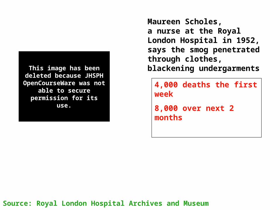
Maureen Scholes, a nurse at the Royal London Hospital in 1952, says the smog penetrated through clothes,blackening undergarments

Source: Royal London Hospital Archives and Museum

4,000 deaths the first week

8,000 over next 2 months

This image has been deleted because JHSPH OpenCourseWare was

not able to secure permission for its use.

Designer Smog Masks - London 1950’s

Davis When Smoke Ran Like Water (2002)

This image has been deleted because JHSPH OpenCourseWare was not able to secure permission for its use.

Air pollution and mortality: Then and now

London, December, 1952 Mortality and PM10 in Chicago, 2000

This image has been deleted because JHSPH OpenCourseWare was

not able to secure permission for its use.

"London "Killer" Smog of 1952" from Environmental Health. Available at: http://ocw.jhsph.edu. Copyright © Johns Hopkins Bloomberg School of Public Health. Creative Commons BY-NC-SA. Adapted from Turco, R. P.

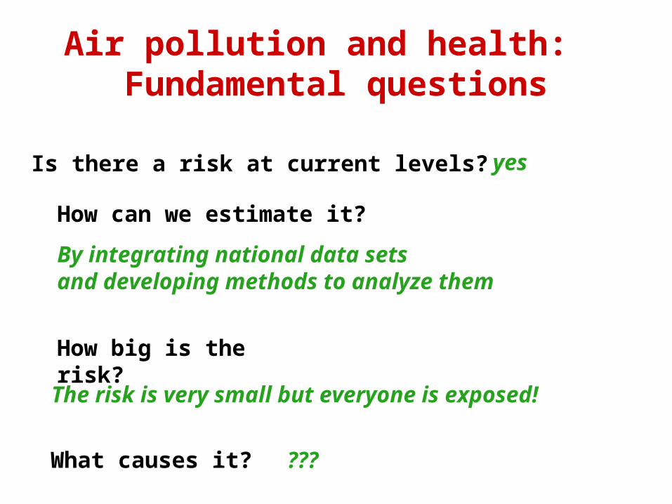
Air pollution and health: Fundamental questions

Is there a risk at current levels?

How can we estimate it?

How big is the risk?

What causes it?

yes

The risk is very small but everyone is exposed!

???

By integrating national data sets and developing methods to analyze them

Bad air day?

Chicago PM2.5 = 10

g /m3

This image has been deleted because JHSPH OpenCourseWare was not able to secure permission for its use.

Bad air day?

Chicago PM2.5 = 20

g /m3

This image has been deleted because JHSPH OpenCourseWare was not able to secure permission for its use.

Bad air day?

Chicago PM2.5 = 30

g /m3

Standard setting process in the US is evidence-based

This image has been deleted because JHSPH OpenCourseWare was not able to secure permission for its use.

National Data Sets

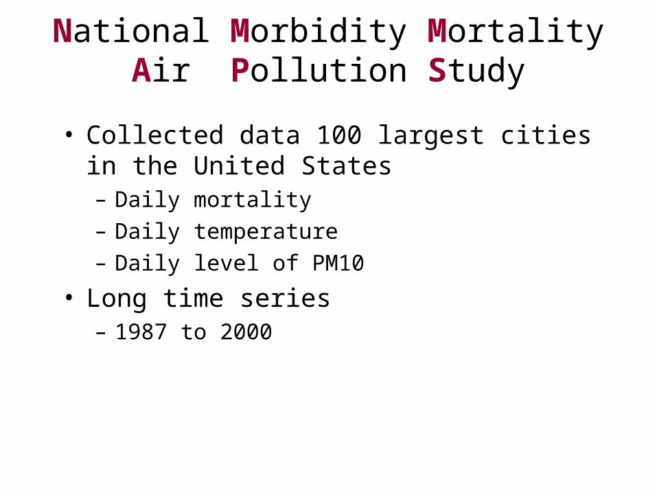
National Morbidity Mortality Air Pollution Study

• Collected data 100 largest cities in the United States– Daily mortality– Daily temperature– Daily level of PM10

• Long time series– 1987 to 2000

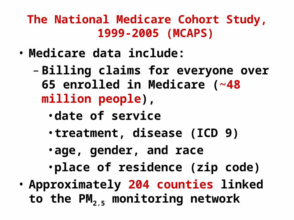
The National Medicare Cohort Study, 1999-2005 (MCAPS)

• Medicare data include: – Billing claims for everyone over 65

enrolled in Medicare (~48 million people), •date of service•treatment, disease (ICD 9)•age, gender, and race•place of residence (zip code)

• Approximately 204 counties linked to the PM2.5 monitoring network

MCAPS study population: 204 counties with

populations larger than 200,000 (11.5 million people)

This image has been deleted because JHSPH OpenCourseWare was not able to secure permission for its use.

Please visit www.biostat.jhsph.edu/MCAPS for maps and other MCAPS information

Daily time series of hospitalization rates and PM2.5 levels in Los Angeles county (1999-2005)

This image has been deleted because JHSPH OpenCourseWare was not able to secure permission for its use.

Please visit www.biostat.jhsph.edu/MCAPS for maps and other MCAPS information

Statistical Ideas

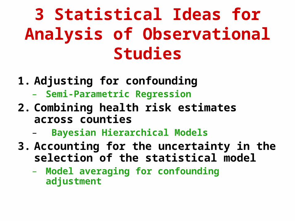
3 Statistical Ideas forAnalysis of Observational

Studies

1. Adjusting for confounding – Semi-Parametric Regression

2. Combining health risk estimates across counties– Bayesian Hierarchical Models

3. Accounting for the uncertainty in the selection of the statistical model– Model averaging for confounding

adjustment

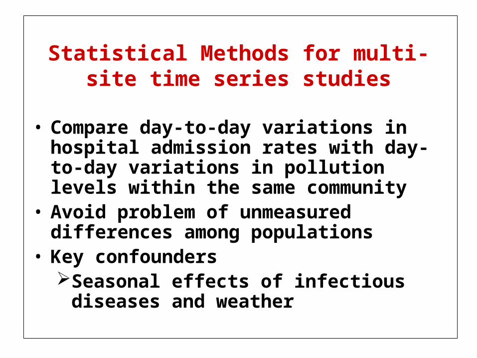
• Compare day-to-day variations in hospital admission rates with day-to-day variations in pollution levels within the same community

• Avoid problem of unmeasured differences among populations

• Key confoundersSeasonal effects of infectious

diseases and weather

Statistical Methods for multi-site time series studies

Statistical Methods

Within city: Semi-parametric regressions for estimating associations between day-to-day variations in air pollution and mortality controlling for confounding factors

Across cities: Hierarchical Models for estimating:– national-average relative rate– exploring heterogeneity of air pollution

effects across the country

Dominici Samet Zeger JRSSA 2000

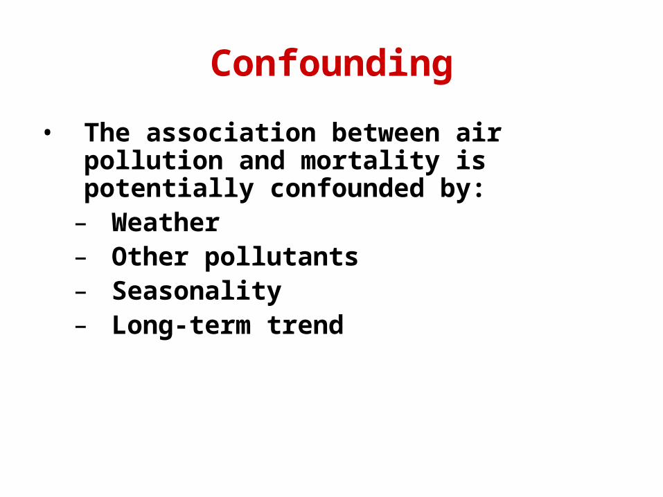
Confounding

• The association between air pollution and mortality is potentially confounded by:

– Weather– Other pollutants– Seasonality– Long-term trend

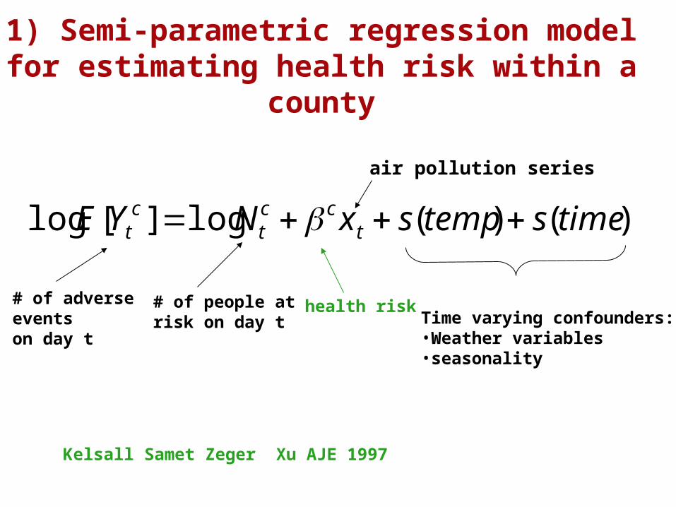
1) Semi-parametric regression model for estimating health risk within a

county

logE[Ytc ] logN t

c cx t s(temp) s(time)

# of adverse events on day t

# of people at risk on day t

health riskTime varying confounders:•Weather variables•seasonality

Kelsall Samet Zeger Xu AJE 1997

air pollution series

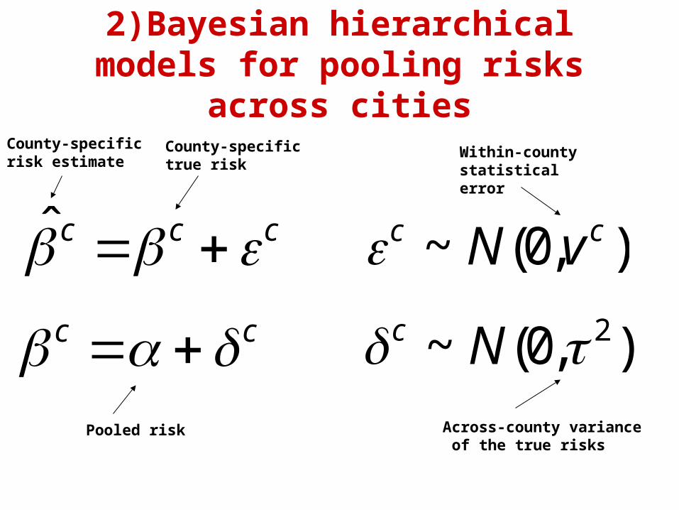
2)Bayesian hierarchical models for pooling risks

across cities

ˆ c c c

c c

c ~ N(0,v c )

c ~ N(0, 2)

County-specific risk estimate

County-specific true risk

Within-county statistical error

Pooled risk Across-county variance of the true risks

3) Do I have the “right” statistical model?

Explore the sensitivity of the risk estimates to the statistical model

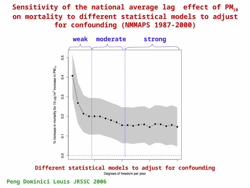
Sensitivity of the national average lag effect of PM10 on mortality to different statistical models to adjust for

confounding (NMMAPS 1987-2000)

Peng Dominici Louis JRSSC 2006

Reported estimate

Different statistical models to adjust for confounding

weak moderate strong

3) Do I have the “right” statistical model?

X

Y

Z1 Z2Z1 is a predictor of YZ2 is a confounder

Regression Models Weights based on prediction(BIC)

Weights based on ability to adjust for confounding

0.9 0.0

0.0 0.9

0.1 0.1

y x 2z2

y x 1z1 2z2

y x 1z1

Estimating risks by averaging across statistical models

3) Model averaging for confounding

adjustment in observational studies • We assign zero weights to models that have

optimal prediction properties but that do not include all the potential confounders

• We identify all the potential confounders by searching for good predictors of the exposure X

• Theoretical results and simulation studies have showed that this approach outperform existing methods to account for model uncertainty

Crainiceanu Dominici Parmigiani Biometrika 2007Wang Crainiceanu Parmigiani Dominici technical report 2007

Biostatistics in Action: The weight of the

evidence

This image has been deleted because JHSPH OpenCourseWare was not able to secure permission for its use.

Full-text available at http://content.nejm.org/cgi/content/abstract/343/24/1742

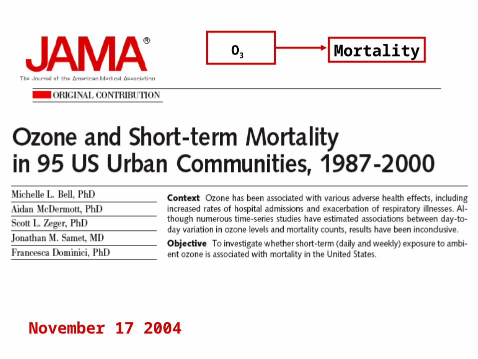
November 17 2004

O3 Mortality

This image has been deleted because JHSPH OpenCourseWare was not able to secure permission for its use.

Full-text available at

http://jama.ama-assn.org/cgi/content/full/292/19/2372

March 8 2005

PM2.5

HospitalAdmissions

This image has been deleted because JHSPH OpenCourseWare was not able to secure permission for its use.

Full-text available at

http://jama.ama-assn.org/cgi/content/full/295/10/1127

The new challenge:Estimating the toxicity of the PM complex mixture

New Scientific Questionsand Statistical Challenges

What are the mechanisms of PM toxicity?

Size? Chemical components? Sources?

New Methods for estimating health effects of complex mixtures

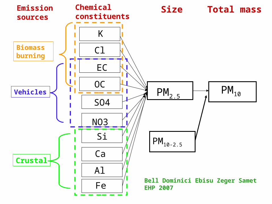
PM2.5 PM10

PM10-2.5

Chemical constituents

Size Total mass

Cl

OC

SO4

Si

K

EC

NO3

Ca

Al

Fe

Biomassburning

Vehicles

Crustal

Emissionsources

Bell Dominici Ebisu Zeger Samet EHP 2007

Lag

% in

crea

se in

adm

issi

on w

i th

a 10

g/m

3 in

crea

se in

PM

0 1 2 0 1 2 0 1 2 0 1 2

-1.5

-1

-0.5

0

0.5

1

1.5

2

PM10 2.5 PM2.5 PM10 2.5

Adjusted by PM 2.5

PM2.5

Adjusted by PM 10 2.5

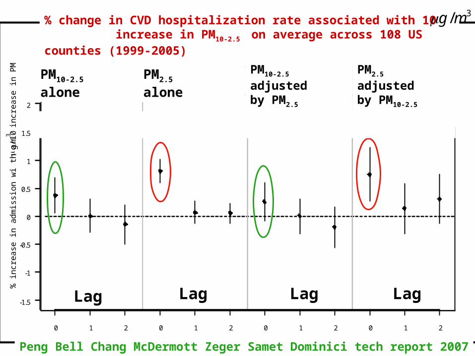
% change in CVD hospitalization rate associated with 10 increase in PM10-2.5 on average across 108 US counties (1999-2005)

g /m3

PM10-2.5

alonePM2.5

alone

PM10-2.5

adjusted by PM2.5

PM2.5

adjusted by PM10-2.5

Lag

Peng Bell Chang McDermott Zeger Samet Dominici tech report 2007

Lag Lag Lag

The policy impact

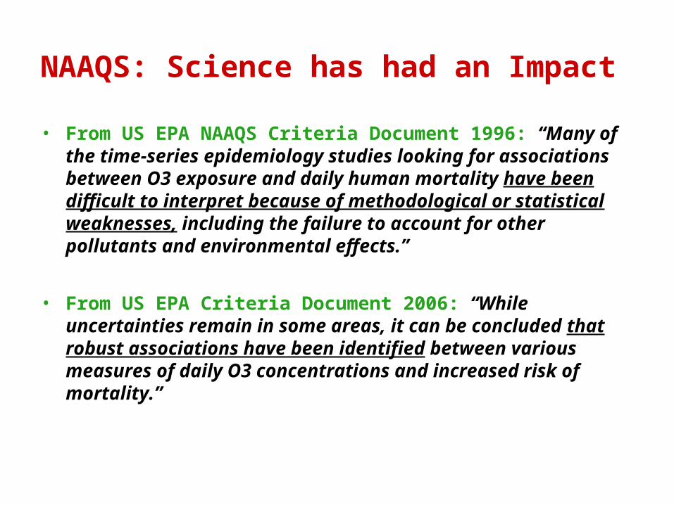
NAAQS: Science has had an Impact

• From US EPA NAAQS Criteria Document 1996: “Many of the time-series epidemiology studies looking for associations between O3 exposure and daily human mortality have been difficult to interpret because of methodological or statistical weaknesses, including the failure to account for other pollutants and environmental effects.”

• From US EPA Criteria Document 2006: “While uncertainties remain in some areas, it can be concluded that robust associations have been identified between various measures of daily O3 concentrations and increased risk of mortality.”

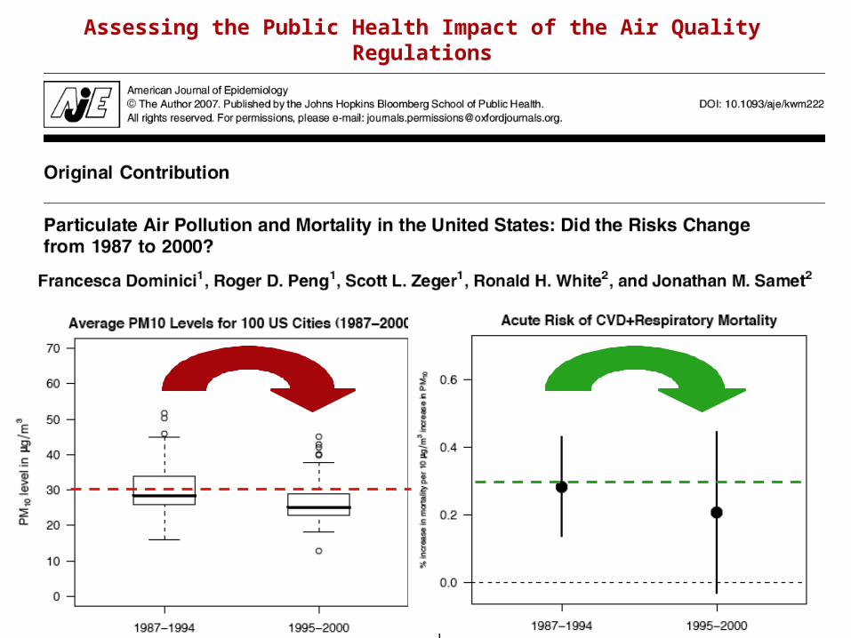
Assessing the Public Health Impact of the Air Quality Regulations

Reproducible research

• We want to reproduce previous findings– “Did you do what you said you did?”

• Test assumptions, robustness of findings; check methodology– “Is what you did any good?”

• Implement and test new methodology– “I can do it better!”

Peng Dominici Zeger AJE 2006

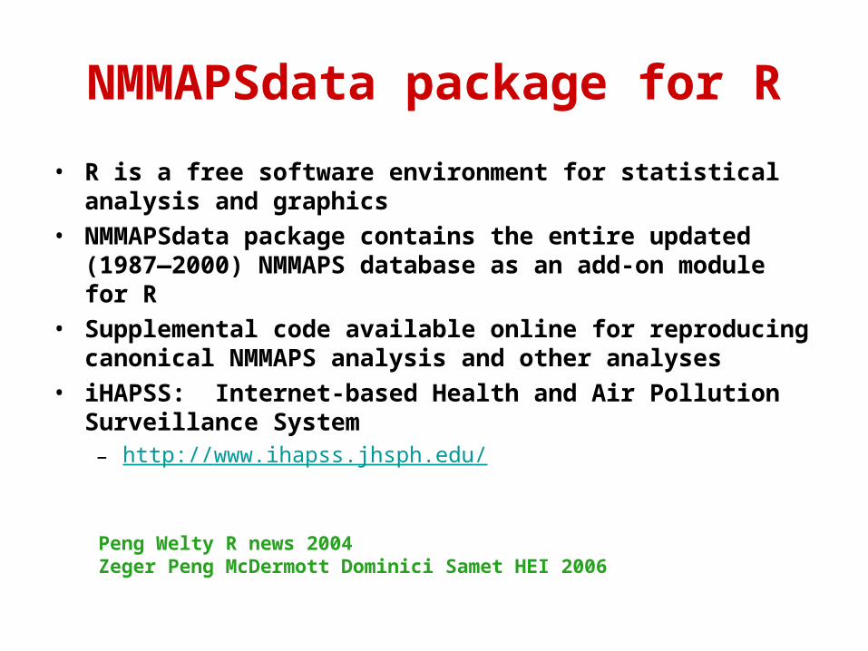
NMMAPSdata package for R

• R is a free software environment for statistical analysis and graphics

• NMMAPSdata package contains the entire updated (1987—2000) NMMAPS database as an add-on module for R

• Supplemental code available online for reproducing canonical NMMAPS analysis and other analyses

• iHAPSS: Internet-based Health and Air Pollution Surveillance System– http://www.ihapss.jhsph.edu/

Peng Welty R news 2004 Zeger Peng McDermott Dominici Samet HEI 2006

A new book to appear this summer…

Environmental Epidemiology with R: A Case study in Air Pollution and Health

Roger Peng & Francesca Dominici

Pen

g &

Dom

inic

i

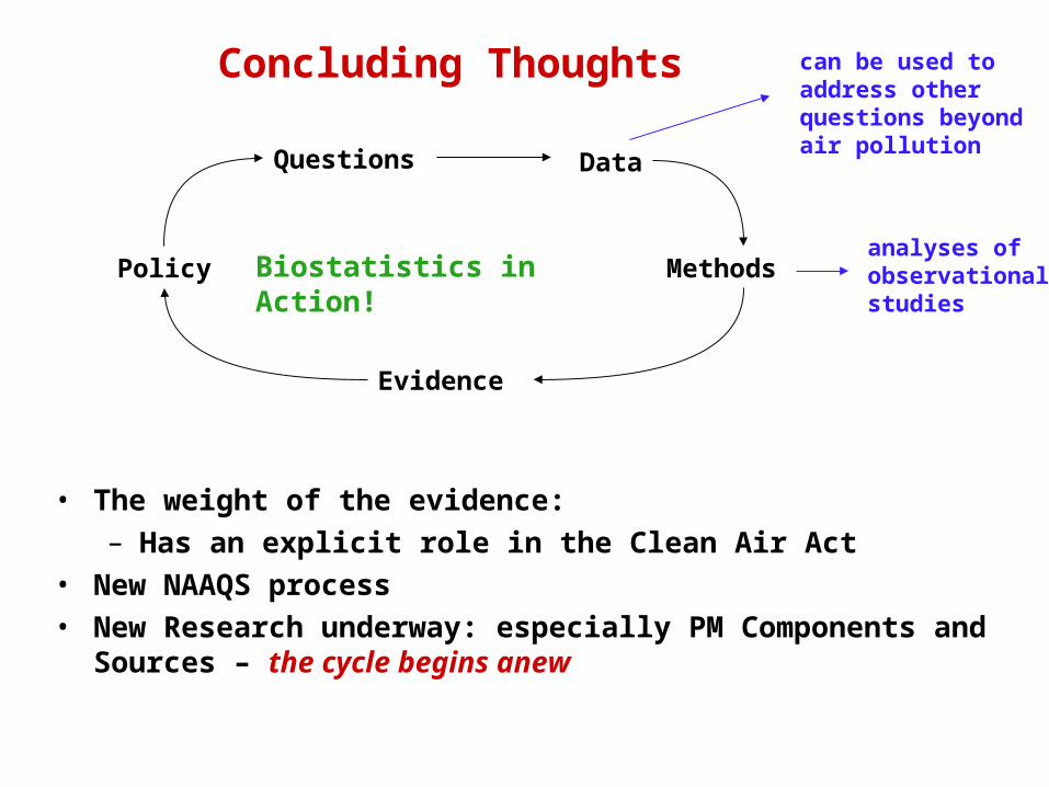
Concluding Thoughts

• The weight of the evidence:– Has an explicit role in the Clean Air Act

• New NAAQS process • New Research underway: especially PM Components

and Sources – the cycle begins anew

Policy

Questions Data

Methods

Evidence

Biostatistics in Action!analyses of observational studies

can be used toaddress otherquestions beyondair pollution

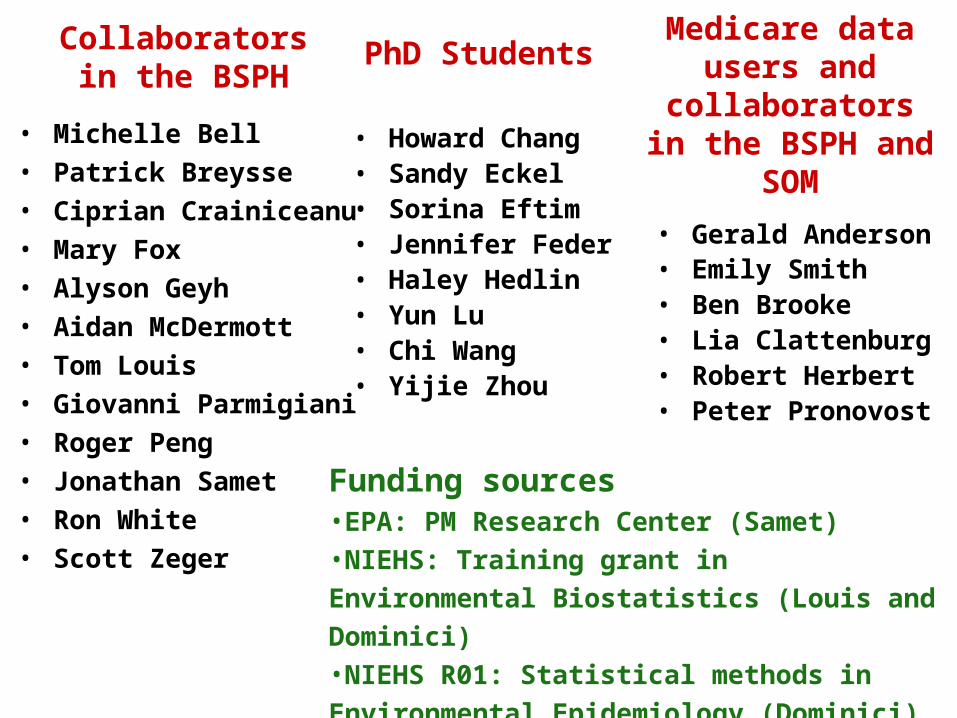
Collaboratorsin the BSPH

• Michelle Bell• Patrick Breysse• Ciprian Crainiceanu• Mary Fox• Alyson Geyh• Aidan McDermott• Tom Louis• Giovanni Parmigiani• Roger Peng• Jonathan Samet• Ron White• Scott Zeger

PhD Students

• Howard Chang• Sandy Eckel• Sorina Eftim• Jennifer Feder• Haley Hedlin• Yun Lu• Chi Wang• Yijie Zhou

Medicare data users and

collaboratorsin the BSPH and

SOM

• Gerald Anderson• Emily Smith• Ben Brooke• Lia Clattenburg• Robert Herbert • Peter Pronovost

Funding sources•EPA: PM Research Center (Samet)•NIEHS: Training grant in Environmental Biostatistics (Louis and Dominici)•NIEHS R01: Statistical methods in Environmental Epidemiology (Dominici)