copyright © 1991, bythe author(s). all rights reserved

Copyright © 1991, by the author(s).All rights reserved.

Permission to make digital or hard copies of all or part of this work for personal orclassroom use is granted without fee provided that copies are not made or distributedfor profit or commercial advantage and that copies bear this notice and the full citation

on the first page. To copy otherwise, to republish, to post on servers or to redistribute tolists, requires prior specific permission.

A CASE STUDY IN APPROXIMATE

LINEARIZATION: THE ACROBOT EXAMPLE

by

Richard M. Murray and John Hauser

Memorandum No. UCB/ERL M91/46

29 April 1991

ELECTRONICS RESEARCH LABORATORY

College of EngineeringUniversity of California, Berkeley

94720

A CASE STUDY IN APPROXIMATE

LINEARIZATION: THE ACROBOT EXAMPLE

by

Richard M. Murray and John Hauser

Memorandum No. UCB/ERL M91/46

29 April 1991

A Case Study in Approximate Linearization:The Acrobot Example

Richard M. Murray* John Hauser*Electronics Research Laboratory Department of EE-Systems

University of California University of Southern CaliforniaBerkeley, CA 94720 Los Angeles, CA 90089-0781

[email protected] [email protected]

29 April 1991

Abstract

The acrobot is a simple mechanical system patterned after a gymnastperforming on a single parallel bar. By swinging her legs, a gymnast is ableto bring herself into an inverted position with her center of mass above thepart and is able to perform manuevers about this configuration. This reportstudies the use of nonlinear control techniques for designing a controller tooperate in a neighborhood of the manifold of inverted equilibrium points.The techniques described here are of particular interest because the dynamicmodel of the acrobot violates many of the necessary conditions required toapply current methods in linear and nonlinear control theory.

The approach used in this report is to approximate the system in such away that the behavior of the system about the manifold of equilibrium pointsis correctly captured. In particular, we construct an approximating systemwhich agrees with the linearization of the original system on the equilibriummanifold and is full state linearizable. For this class of approximations,controllers can be constructed using recent techniques from differential geometric control theory. We show that application of control laws derived inthis manner results in approximate trajectory tracking for the system undercertain restrictions on the class of desired trajectories. Simulation resultsbased on a simplified model of the acrobot are included.

'Research supported in part by an IBM Manufacturing fellowship and the NationalScience Foundation, under grant IRI-90-14490.

*Fred O'Green Assistant Professor of Engineering

1 INTRODUCTION

Figure 1: Acrobot: an acrobatic robot. Patterned after a gymnast on aparallel bar, the acrobot is only actuated at the middle (hip) joint; the firstjoint, corresponding to the gymnast's hands on the bar, is free to spin aboutits axis.

1 Introduction

Recent developments in the theory of geometric nonlinear control providepowerful methods for controller design for a large class of nonlinear systems.Many systems, however, do not satisfy the restrictive conditions necessaryfor either full state linearization [7, 5] or input-output linearization withinternal stability [2]. In this paper, we present an approach to controller design based on finding a linearizable nonlinear system that well approximatesthe true system over a desirable region. We outline an engineering procedure for constructing the approximating nonlinear system given the truesystem. We demonstrate this approach by designing a nonlinear controllerfor a simple mechanical system patterned after a gymnast performing on asingle parallel bar.

There has been considerable work in the area of system approximationincluding Jacobian linearization, pseudo-linearization [10, 12], approximation with a nonlinear system [8], and extended linearization [1]. Much ofthe work on system approximation has been directed toward analysis andthe development of conditions that must be satisfied by the approximatesystems rather than on the explicit construction of such approximations.Notable exceptions include the standard Jacobian approximation and therecent work of Krener using polynomial system approximations [9]. Wangand Rugh [12] also provide an approach for constructing configuration sched-

1 INTRODUCTION 2

uled linear transformations to pseudo-linearize the system (note that thisapproach provides a family of approximations rather that a single systemapproximation). Rather than using polynomial systems or families of linearsystems to approximate the given system, we approximate the given nonlinear system with a single nonlinear system that is full state linearizable.

We use as a guiding example the problem of controlling the acrobot (foracrobatic-robot) shown in Figure 1. The acrobot is a highly simplified modelof a human gymnast performing on a single parallel bar. By swinging her legs(a rotation at the hip) the gymnast is able to bring herself into a completelyinverted position with her straightened legs pointing upwards and her centerof mass above the bar. The acrobot consists of a simple two link manipulatoroperating in a vertical plane. The first joint (corresponding to the gymnast'shand sliding freely on the bar) is free to rotate. A motor is mounted at thesecond joint (between the links) to provide a torque input to the system(corresponding to the gymnast's ability to generate torques at the hip). Alife size acrobot is currently being instrumented for experimentation at U.C.Berkeley.

The eventual goal in controlling this system is to precisely execute realistic gymnastic routines. Our modest initial goal is to understand and designcontrollers capable of system control in a neighborhood of the manifold ofinverted equilibrium positions. That is, we would like to have the acrobotfollow a smooth trajectory while inverted, such as that shown in Figure 2.

This report presents a detailed study of the stabilization and trackingfor the acrobot. We begin with a complete, mathematical description ofthe system in Section 2. The application of standard control techniques tothe acrobot is studied in Section 3. Section 4 briefly introduces the theoryof approximate linearization and develops a family of nonlinear controllersusing this theory. A comparison of these controllersagainst a standard linearcontroller is given in Section 5. Finally, we discuss more general nonlinearcontrol problems and how our results for the acrobot can be applied to them.

The application of the methods presented here require substantial algebraic computation. We have used Mathematica [13] to perform much of ourcomputation for us. We list in the body of this paper the specific Mathematica files which were used to obtain or check indicated results. The listingsfor these files can be found in the appendix.

1 INTRODUCTION

Figure 2: Motion of the acrobot along the manifold of inverted equilibriumpositions.

2 SYSTEM DESCRIPTION

2 System description

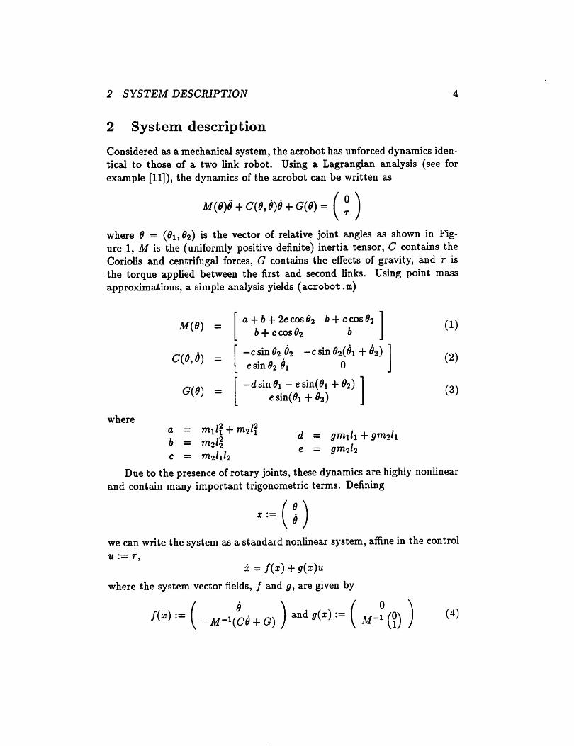
Considered as a mechanical system, the acrobot has unforced dynamics identical to those of a two link robot. Using a Lagrangian analysis (see forexample [11]), the dynamics of the acrobot can be written as

M(0)0 + C(0,0)0 + G(0) =0

where 0 —(0i,02) is the vector of relative joint angles as shown in Figure 1, M is the (uniformly positive definite) inertia tensor, C contains theCoriolis and centrifugal forces, G contains the effects of gravity, and r isthe torque applied between the first and second links. Using point massapproximations, a simple analysis yields (acrobot.m)

where

M(0) =

C(0,0) =

G{9) =

a + b -f 2c cos 92 b + c cos 9<ib + c cos 02 &

-csin 02 02 -csin 02(0i + 02)c sin 02 0i 0

-dsin 0i - e sin(0i + 02)esin(0i-r-02)

a — m\l\ + 7712/16 = 7712/2c = 7712/1/2

Due to the presenceof rotary joints, these dynamics are highly nonlinearand contain many important trigonometric terms. Defining

d = gmili + gmil\e = #7712/2

x :=

(1)

(2)

(3)

we can write the system as a standard nonlinear system, affine in the controlu := r,

x = f(x) + g(x)u

where the system vector fields, / and g, are given by

0 \

M:= ( -M-\C9 +G) ) and 9{X) := ( M-i (?) (4)


Non-inverted positions

Inverted positions

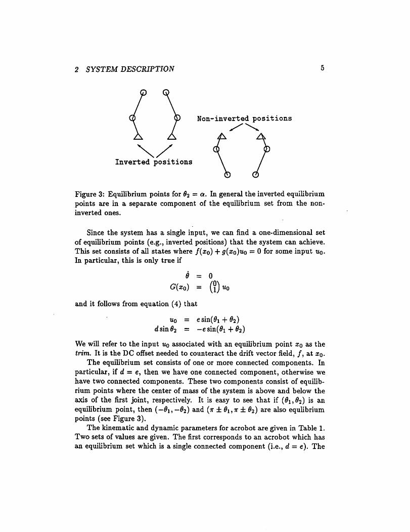
Figure 3: Equilibrium points for 02 = a. In general the inverted equilibriumpoints are in a separate component of the equilibrium set from the non-inverted ones.

Since the system has a single input, we can find a one-dimensional setof equilibrium points (e.g., inverted positions) that the system can achieve.This set consists of all states where /(xo) + g(xo)uo = 0 for some input uq.In particular, this is only true if

0 = 0

G(xQ) = (J)ttoand it follows from equation (4) that

wo = esin(0i + 02)d sin 02 = -esin(0i+ 02)

We will refer to the input uq associated with an equilibrium point xq as thetrim. It is the DC offset needed to counteract the drift vector field, /, at xq.

The equilibrium set consists of one or more connected components. Inparticular, if d = e, then we have one connected component, otherwise wehave two connected components. These two components consist of equilibrium points where the center of mass of the system is above and below theaxis of the first joint, respectively. It is easy to see that if (0i,02) is anequilibrium point, then (-0i, -02) and (ir ± 0i,7r ± 02) are also equlibriumpoints (see Figure 3).

The kinematic and dynamic parameters for acrobot are given in Table 1.Two sets of values are given. The first corresponds to an acrobot which hasan equilibrium set which is a single connected component (i.e., d = e). The


Parameter Units Balanced Actual

Value Value

h m 1/2 1/2h m 1 3/4

mi kg 8 7

7712 kg 8 8

9 m/s2 10 9.8

Table 1: Acrobot parameters. The balanced values correspond to a versionof the acrobot which has a connected equilibrium set.

2.0 -

^ 0.0"5

Balanced Parameter*

-2.0 0.0 2.0

Inner Joint angle. 8,

4.0Actual parameters

-2.0 0.0 2.0

Inner joint angle. 0(

Figure 4: Equilibrium points for acrobot. The left figure is the equilibriumset using the balanced parameter values, the right plot using the actualparameter values.

second set of values is the approximate parameter values for the physicalsystem at U.C. Berkeley. We have rounded units to rational numbers toease the computational burden. We shall use the former ("balanced") valuesunless otherwise noted.

The equilibrium points for the two sets of parameters are shown in Figure 4. For the "balanced" parameter values, the equilibrium set consistsof all 0i + \92 = 0, 0i + |02 = 7T, and 02 = ±t. This last set of pointscorresponds to the case where the center of mass of the system is coincidentwith the axis of the first joint, and hence every value of 9\ corresponds toan equilibrium configuration. Note also that there is a gap in the range of01 for which the "actual" system may be balanced.

3 LINEARIZATION TECHNIQUES 7

3 Linearization techniques

In this section we explore the application of linearization techniques to thecontrol of the acrobot. We distinguish between two different linearizationmethods. The first is linearization about a point, in which we approximatethe vector fields / and g by their linearizations about an equilibrium point.If the linearization is stabilizable to that equilibrium point, then in a suitably small neighborhood the nonlinear system can also be stabilized (bylinear feedback). A more recent technique is feedback linearization (see, forexample, Isidori [6]). This method uses a change of coordinates and nonlinear state feedback to transform the nonlinear system description to a linearone (in the new coordinates).

3.1 Linearization about an equilibrium point

If we let (a?o» ^o) GR4 x R denote an equilibrium point for the acrobot, thelinearization about (xo,«o) is given by

z — Az + bv

wherez = x — Xo v = U — Uq

A=& (/(*) +9(x)u)\{x0iUo) b=g(x0)We refer to this method of linearization as Jacobian linearization since it

replaces the system vector fields by their Jacobians with respect to x andu evaluated at a point. The linearized system is completely controllable ifand only if

det 6 Ab •-. An~xb ] #0 (5)

It is straightforward to check that the acrobot linearization is completelycontrollable in a neighborhood of 0i = 02 = 0, 0i = 02 = 0 (straight up). Atthis point

A =

0 0 1 0

0 0 0 1

ll

L ii

_ amihmi

g(limi+l1m2+hm.2)

0

0

0

0llhmi

6 =

0

0

l\l2m\^m1+(li+l2)2m7

3 LINEARIZATION TECHNIQUES

O

«

C)

A

\A

Figure 5: Gravity coupling in the acrobot. By moving the center of mass toone side of the vertical axis, we can cause the entire mechanism to rotate.

By smoothness, it follows that the system is controllable in a neighborhoodof the origin. We defer the analysis of points where controllability is lostuntil later in this section.

Controllability for the acrobot can be givenphysicalinterpretation. Consider the case when the mechanism is pointed straight up, with its center ofmass directly above the pivot point (see Figure 5). We have direct controlof the relative angle of the second link. By moving the second link to theleft or right, we can force the center of mass to lie on either side of the pivotpoint and thus force the whole mechanism to rotate. This use of gravity iscrucial in achieving control since equation (5) is not satisfied if g = 0 (Ab iszero).

A second effect which occurs is inertial coupling between the first andsecond links. Since the motor exerts a torque on the second joint relativeto the first joint, pushing the second joint in one direction causes the firstjoint to move in the opposite direction. This phenomenon is seen in thelinear model by the presence of a right half plane zero; the transfer functionbetween the hip torque and the angle of the first joint (using the balancedparameter values from Section 2) is:

3(*+2>/D (* - VD4(s4 - 60s2 + 400)

Solving for the poles of this transfer function verifies that the acrobot isopen loop unstable.

We now return to the question of controllability and investigate equilibrium points at which the linearization is notcontrollable. Figure 6 shows aplot of the determinant of the controllability matrix in equation (5) versus

3 LINEARIZATION TECHNIQUES

Figure 6: Determinant of controllability matrix versus 02- The plot on theleft corresponds to the balanced parameters and the plot on the right to theactual parameters.

the hip angle of the acrobot. We see that the system is controllable exceptat points where 02 = ±tt. Physically this configuration corresponds to thesecond link of the acrobot pointing back along the first. In this configuration, the balanced acrobot can swing freely about the axis of the first linkand remain in an equilibrium position.

So far our discussion has centered about using a linear controller for stabilization; our real interest is in trajectory tracking. We begin by reviewingtrajectory tracking for a linear system

x = Ax + bu

We assume the system is completely controllable and we wish to track adesired state trajectory X&. Without loss of generality we can assume that(A, 6) are in controllable canonical form, i.e. a chain of integrators. In thiscase the system can be written as

X\ — x2

£2 = £3

Xn_i — xn

xn = u

where we have placed all poles at the origin to simplify notation.If xd(-) is a desired trajectory which satisfies xd = Axd -f bud for some

ud (i.e., xd is achievable) then we can follow this trajectory by using

u = x:


when xd(Q) —x(0). This choice of inputs corresponds to injecting the properinput at the end of the chain of integrators which model the system.

To achieve trajectory tracking even if our initial condition does not satisfy xd(0) = x(0) we introduce the feedback control law

u = i* + ai(*2 - xn) + •••+ an{x{ - xx)

and the error system satisfies

e(n> + aie(n_1) + •••+ ane = 0 e = x — x

By choosing the a's so that the resulting transfer function has all of its polesin the left half plane, e will be exponentially stable to 0 and the actual statewill converge to the desired state.

In the case of a linearized system, the linearization may not be a good approximation to the system for arbitrary configurations. Since we linearizedabout a single point, we can only guarantee trajectory tracking in a sufficiently small ball of states about that point. There are several methodsfor circumventing this problem; one of the most common is gain scheduling.To use gain scheduling, we design tracking controllers for many differentequilibrium points and choose our gains based on the equilibrium point(s)to which we are nearest. In fact, this can be done in a more or less continuous fashion using a technique called extended linearization [12]. The basicrestriction is that the desired reference trajectory must be slowly varying.

3.2 Feedback linearization

Given a nonlinear system

x = f(x) + g(x)u (6)

it is sometimes possible to find a change of coordinates f = <f>{x) and acontrol law u —a(x) + (3(x)v such that the resulting dynamics are linear:

f = A£ + bv

In such cases we can control the system by converting the desired trajectory or equilibrium point to our new coordinates, calculating the control vin the that space, and then pulling the control back to the original coordinates. If such a change of coordinates and feedback exists, we say that (6)is input/state linearizable.


The conditions under which a general nonlinear system can be convertedto a linear one as described above were formulated independently by Jakub-cyzk and Respondek and Hunt, Su and Meyer. For the single input case,the conditions are given by the following theorem.

Theorem 1 ([7, 5]) The system (6) is input/state linearizable in an openset U if and only if

(i) dim span{<7, adjg, •••,aav}~1g}(x) = nyVx £ U(ii) span{<7, adjg, •••, adl~2g} is an involutive distribution on U

where acfjg is the iterated Lie bracket [/,•••, [f,g] •••]•

The first condition is a controllability test and agrees with the linearizationwhen evaluated at an equilibrium point. The importance of the secondcondition is more subtle.

If condition (ii) is satisfied, then there exists a smooth h:Rn —*• R suchthat

dh

dxg ad/$f...adr-20 =0 (7)

This can be seen by applying Frobenius7 theorem: since the distribution isinvolutive, there exists a foliation such that the tangent space to each leafof the foliation is spanned by the distribution restricted to that leaf. Sincethe leaves have dimension n —1, there exists a scalar valued function h suchthat the leaves are defined by h~1(a) for a € R. Equation (7) is essentiallysaying that the gradient of h is perpendicular to the leaves.

The standard approach in feedback linearization is to use h to define therequired change of coordinates. For single input systems we define

<f>i{x) = h(x)<k(x) = Vflh(x)

where Lfh = |£/ is the Lie derivative of h in the direction /. The condition in equation (7) guarantees that the input will not appear until the nthderivative. Setting f = <f>(x), our new equations are

fi = fi+i i=l,---,n-l£n = a(x) + b(x)u

and by using u = b~1(—a + v) we have a linear system (in Brunowskycanonical form).


Trajectory tracking for such a system is exactly as in the linear case.However, since we have converted the model to a linear one instead of approximating it, we do not need to stay close to any particular equilibriumpoint. Thus in an open set U in which the feedback linearizability equationsare satisfied, we can achieve exponential trajectory tracking.

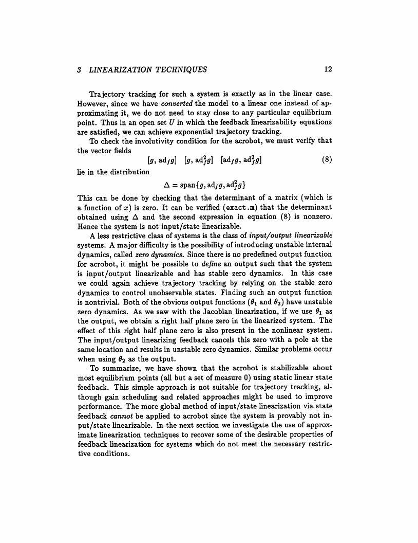
To check the involutivity condition for the acrobot, we must verify thatthe vector fields

[9, ad/y] [g, adjflr] [&dfg, ad2^] (8)lie in the distribution

A = span{p,ad/^,adyfif}

This can be done by checking that the determinant of a matrix (which isa function of a;) is zero. It can be verified (exact.m) that the determinantobtained using A and the second expression in equation (8) is nonzero.Hence the system is not input/state linearizable.

A less restrictive class of systems is the class of input/output linearizablesystems. A major difficulty is the possibility of introducing unstable internaldynamics, called zero dynamics. Since there is no predefined output functionfor acrobot, it might be possible to define an output such that the systemis input/output linearizable and has stable zero dynamics. In this casewe could again achieve trajectory tracking by relying on the stable zerodynamics to control unobservable states. Finding such an output functionis nontrivial. Both of the obvious output functions (0i and 02) have unstablezero dynamics. As we saw with the Jacobian linearization, if we use 0i asthe output, we obtain a right half plane zero in the linearized system. Theeffect of this right half plane zero is also present in the nonlinear system.The input /output linearizing feedback cancels this zero with a pole at thesame location and results in unstable zero dynamics. Similar problems occurwhen using 02 as the output.

To summarize, we have shown that the acrobot is stabilizable aboutmost equilibrium points (all but a set of measure 0) using static linear statefeedback. This simple approach is not suitable for trajectory tracking, although gain scheduling and related approaches might be used to improveperformance. The more global method of input/state linearization via statefeedback cannot be applied to acrobot since the system is provably not input/state linearizable. In the next section we investigate the use of approximate linearization techniques to recover some of the desirable properties offeedback linearization for systems which do not meet the necessary restrictive conditions.

4 APPROXIMATE LINEARIZATION 13

4 Approximate linearization

In the previous section we showed that the acrobot dynamics are not exactlylinearizable by state feedback. In this section we apply the technique ofapproximate linearization to the acrobot. Briefly, we wish to find vectorfields / and g which are close to our original vector fields but which satisfythe exact Unearizability conditions. We then proceed to design a controllerfor the approximate system and apply it to the actual system.

The usual method of approximate linearization is slightly complicatedin the case of the acrobot for two reasons: we do not have a natural outputfunction and we wish to track trajectories near a manifold of equilibriumpoints rather than near a single point. This chapter presents a methodologyfor designing a controller for a system of this type. Briefly, we will proceedin the following manner:

1. Parameterize the controllable equilibrium manifold, £, as (xi, 0, •••, 0).

2. Construct a smooth output, h(x), such that the linearized system ateach equilibrium point has relative degree n.

3. Using h, construct approximate vector fields / and g such that theyapproximate / and g along the equilibrium manifold and the approximate system is exactly linearizable.

4. Using / and g, design a tracking controller for the approximate systemand apply the resulting controller to the original system.

We begin with a brief review of approximation theory using the presentationin Hauser et. al. [3] as a guide.

4.1 Review of approximation theory

We consider systems of the form

i = f(x) + g(x)u , .y = h(x) w

The system is input/output linearizable with relative degree n in a neighborhood U if and only if for all x € U

(i) LgLif1h(x) = 0 i =l,...,r-l(ii) LgLnf1h(x)^0


where Ljh = |§/ is the Lie derivative of h in the direction /. Theseconditions are equivalent to the exact linearization conditions in Theorem 1 of the previous section. That is, || annihilates the distribution{(j,ad/(7,«««,ady~2<7}. As before, we use the output £ = h(x) and its firstn derivatives to define a new set of coordinates. Using this new set of coordinates, the input/output map is given by the linear transfer functionl/sn.

If the input/output conditions are not satisfied, then we can still usethis basic construction as a method for generating approximate vector fieldswhich do satisfy the conditions, at least in a neighborhood of a controllableequilibrium point. Since the behavior of the nonlinear system about anequilibrium point is determined by its linearization, any approximate systemshould agree with the linearized system at an equilibrium point (x0,uo).That is, the approximate vector field f + gu should agree to first order withthe original vector field / -f gu, when evaluated at the equilibrium point. Inparticular, this implies that the relative degree of any approximate systemshould agree with the relative degree of the linearization. This motivatesthe following definition: the linearized relative degree of a nonlinear systemin a neighborhood of an equilibrium point xq is the relative degree of thelinearization about xq. We use this concept to construct an approximatesystem which has relative degree equal to the linearized relative degree ofthe original system.

A key concept is that of higher order. A function tp(x) is said to behigher order at xo if the function and its first derivative vanish at xq. Moregenerally, a function is order k at xq if the function and its first k derivativesvanish at $o, and first order if only the function itself is zero at xq.

Let xo be an equilibrium point of a nonlinear system with uo the inputrequired to hold the system at the equilibrium point. Suppose the linearizedrelative degree of the system about xq is n. Then we can define an approximate system in a neighborhood of (xq, «o) as follows: set

4>i(x) = h(x) - i>0(x)

where Vo is any function that is higher order at xo. For t = 2, • • •,n, set

<f>i(x) = Ls<j>i-i(x) + uQLg<t>i-i(x) - ipi-i(x)

where ^,(x) is higher order at xo. It can be shown that <f> is a local diffeo-morphism and hence defines a valid change of coordinates. If we write the

4 APPROXIMATE LINEARIZATION

6

/TT/TT/fr/

i>(x,y)higher order nonlinear terms

15

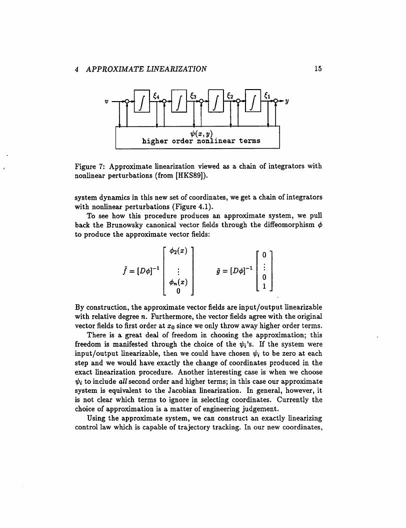
Figure 7: Approximate linearization viewed as a chain of integrators withnonlinear perturbations (from [HKS89]).

system dynamics in this new set of coordinates, we get a chain of integratorswith nonlinear perturbations (Figure 4.1).

To see how this procedure produces an approximate system, we pullback the Brunowsky canonical vector fields through the diffeomorphism <j>to produce the approximate vector fields:

-lf = [D4>]

<h(x)

<f>n(x)0

-l9 = [D4>\

By construction, the approximate vector fields are input/output linearizablewith relative degree n. Furthermore, the vector fields agree with the originalvector fields to first order at xo since we only throw away higher order terms.

There is a great deal of freedom in choosing the approximation; thisfreedom is manifested through the choice of the ^t's. If the system wereinput/output linearizable, then we could have chosen ifii to be zero at eachstep and we would have exactly the change of coordinates produced in theexact linearization procedure. Another interesting case is when we chooseij>i to include all second order and higher terms; in this case our approximatesystem is equivalent to the Jacobian linearization. In general, however, itis not clear which terms to ignore in selecting coordinates. Currently thechoice of approximation is a matter of engineering judgement.

Using the approximate system, we can construct an exactly linearizingcontrol law which is capable of trajectory tracking. In our new coordinates,


f = <f>(x), the system has the form

& = Zi+i + 4>i(x) + #i(x)(u - u0)in = Lf<f)n(x) + Lg4>n(x)u + lj>n(x) + 9n(x)(u - Uq)y = 6 + 4>o(x)

where each 0,- is at least uniformly first order at xo- With analogy to theexact linearization case, we choose

u=j-itm (-WnW +y™ +«»-i(»in"l) -£») +•••+«o(w - &))LgVnW ^ '(10)

where sn + an_isn_1 H h «o has all its zeros in the open left half plane.Let

and define the tracking error as

This error vector encodes the deviation of the actual system trajectory fromthe desired trajectory of the approximate system.

For € sufficiently small and desired trajectories which are e-near xo andsufficiently slow, the control law (10) results in approximate tracking ofthe desired trajectory [3]. Thus we can approximately track any trajectorywhich remains close to the equilibrium point and is slowing varying. A moreexplicit (and more general) formulation is presented in Section 4.4.

4.2 The equilibrium manifold

In our application, we are not interested in motion near a single equilibriumpoint, but rather motion near a set of equilibrium points. Given a generalsingle input system, the equilibrium points are those xo for which /(xo) +g(xo)uo = 0 for some uq € R. We define S to be the set of all equilibriumpoints, xo, such that the linearized system is controllable about xo.

Theorem 2 S is a manifold of dimension 1.

Proof. Consider first the set £XjU of all pairs (xo, wo) such that /(xo) +<jr(xo)wo = 0 and the system is controllable at xo. Controllability is determined by taking the determinant of a set of smooth functions and hence


•Xi

x£

Figure 8: Projection of the equilibrium points onto the state space [10].

there exists and open ball N B (xo,wo) such that all equilibrium points(x', u') G N are also controllable. Let U be the union of all such N over£x,u. Then U is open and £x,u C U. Define the map F: U C Rn+1 -* Rngiven by F:(x,u) \-+ f(x) + g(x)u. At any controllable equilibrium point,F(xo,uo) = 0 and the Jacobian of i*1,

DF(x0,u0) = (Df(x0) + u0Dg(x0),g(xo)) = (A0,60),

is full rank. Hence 0 is a regular value of F and ir_1(0) = £X)U is a subman-ifold of Rn -f 1 of dimension (n + 1) - n = 1.

It remains to show that the projection is also a manifold. There are twothings that can go wrong: the manifold can be tangent to the projectiondirection or the manifold can cross over itself. These situations are shown

in Figure 8. These singularities can only occur if uo cannot be written as afunction of xo. However, at any equilibrium point

f(xo) + g(x0)u0 = 0

and wo is not unique only if </(xo) = 0. This contradicts controllability andhence uq is a unique function of xo and neither of the situations in Figure 8can occur. D

We call S the controllable equilibrium manifold and will often refer to itsimply as the equilibrium manifold (as opposed to the set of all equilibrium


or operating points). In general £ consists of one or more connected components. For the acrobot there are always two components, consisting of theinverted and non-inverted equilibrium points.

While motion on the controllable equilibrium manifold is not possible(since by definition x = 0 on the manifold), motion near the manifold canbe achieved. In constructing an approximate system, we wish to do so in away that keeps the approximation close at equilibrium points. Thus we wantto throw away terms which are higher order on the equilibrium manifold (i.e.,terms whose value and first derivative vanish on S) while keeping terms thatvary along the equilibrium manifold.

In order to construct such an approximation, it is convenient to changecoordinates so that the equilibrium manifold has a simple form. A particularly convenient choice of coordinates is one in which points on the equilibrium manifold have the form (xi, 0, • ••, 0). We can always find a parameterization of the equilibrium manifold which has this form in a neighborhoodof a controllable equilibrium point, since £ is a one dimensional manifold.

For the acrobot, we have chosen to parameterize the equilibrium manifold using the hip angle. For the second configuration variable we use theangle of the center of mass of the system—this must be zero at all invertedequilibrium points since the center of mass must lie directly above the axisof the first link. We complete the state with the velocities of the two configuration variables. These calculations are contained in (equilibrium.m).The resulting change of coordinates (see Appendix A) is:

Xi = 02

*2 = 01 +

*3 = Xi

X4 = x2

e sin 02y/d* + e2 + 2edcos92

Other parameterizations are possible. For example, one might choosethe x and y components of the system center of mass as the configurationvariables. Unfortunately, the parameterization is singular about the straightup position, just as it is for a two-link robot manipulator. Another advantageof the parameterization we chose is that it simplifies some of the calculations.In particular, for the balanced system parameters mentioned in Section 2,the angle of the center of mass is simply 0i + \9% whereas x^ and ycminvolve trigonometric functions. This is the original motivation for definingthe "balanced" set of parameters.


4.3 Constructing an (artificial) output function

In the approximation theory presented above, an output function was usedto construct the approximate system. In some applications, the system possesses a natural output function that can be used for this purpose. However,in the case of the acrobot, no suitable output function is given so we mustconstruct one. In this section we present a technique for doing so. As usual,we begin by considering the linear case.

Suppose we are given a controllable linear system

x = Ax + bu

and we are asked to find an output

y = ex

which is suitable for stable trajectory tracking. By this we mean that it iseasy to design a controller to make y(t) track a desired trajectory yd(t) whilemaintaining internal stability of the system. If the system is in Brunowskyform (i.e., a chain of integrators), then a natural output function is theoutput from the last integrator. This insures that the system has no zerossothat y(t), y(t),..., y^n~^(t) can beused as the n coordinates ofthe systemstate. In particular, if the output y(t) converges to a constant value, thenthe system will converge to an equilibrium point.

To construct this output when the system (A, b) is not in Brunowskycanonical form, we note that the relative degree of the system is given bythe largest r such that

cAi~1b = 0 t = l,...,r-lcAr~lb # 0

Since we want the relative degree to be n (no zeros), we require that

b Ab ••• An~2l = 0. (11)

Thus, any c ^ 0 in the (1-dimensional) null space indicated by equation (11)defines an output such that the system (c, A, 6) has relative degree n.

We now return to the nonlinear system

x = f(x) + g(x)u


with the goal of constructing an output

y = h(x)

to use in constructing an approximate system for control design. If the system with output is input/output linearizable with relative degree n aroundxo then the system is linearly controllable and satisfies the nonlinear analogto (11) given by

= 0—[g ad/i7 ... ad? 2<for all x in a neighborhood of xo- In other words, the system is input/statelinearizable—it satisfies the conditions of Theorem 1. Since many systemssuch as the acrobot are not input/state linearizable, we look to approximation. Our problem is one of finding a function h and approximate vectorfields / and g such that

^[g ad7£ ... ad^]=0 (12)for all x in a neighborhood of xo or, more generally, in a neighborhood ofthe equilibrium manifold.

Since it is extremely difficult to directly modify the vector fields /, g sothat the system is exactly input/state linearizable, we will first construct theoutput function h and then use the approximate linearization methodologyto construct / and g. The basic idea is to find a function h that satisfiesequation (.12) at each point on the equilibrium manifold. Provided that theoriginal and approximate systems agree to first order on the equilibriummanifold, the ad-chains of the two systems will span the same subspace ateach point on the equilibrium manifold, that is,

span{#, ad/0, •••, ad""2^} =span{£, adj£, •«•, &tfj~2g}

for x G £. In fact, these calculations can be done directly with the linearization of the original system on the equilibrium manifold. This point issomewhat subtle, so we describe it in detail.

We will assume that coordinates have been chosen such that the equilibrium manifold £ has been straightened out so that each x G £ has the form(x1}0,.. .,0). Let xe(xi) and ue(x\) denote the state and control for eachequilibrium point (xi, 0,..., 0) on £, that is,

xe(xi) = (xi,0,...,0)


and we(«) is such that

f(xe(xi)) + g(xe(xi))ue(xi) = 0

for each xi such that xe(xi) G £.Suppose, at first, that we trim the drift vector field

f(x):=f(x) + g(x)uc(x)

where uc(-) is any control satisfying uc(xc(xi)) = ue(x\). The linearizationof the trimmed system along the equilibrium manifold is then given by

i = A(x\)z + b(x\)v

where

^(*i) •= ^e(xi)) +uc(xe(x1))^(xe(x1)) +g(xe(x1))^(xe(xl))= E(*e(*l)) + We(Xi)|j(xe(x1)) + <7(*c(xi))^f(xe(Xi))

6(xi) := g(xe(xi))

In this case it is easy to verify that

ad^(xe(xi)) = (-i(xi))J6(xi)

Thus, letting c(-) be the derivative of the yet to be constructed outputfunction h along the equilibrium manifold,

c(xi) := ^(xe(xi)),

equation (12) (for the trimmed system) evaluated along £ takes the form

c(xi)[6(x!) I(xi)6(xi) ••• i(xi)n"26(xi) ] =0 (13)

The equation has a smooth solution c(-) on £ since the system is, by definition, linearly controllable at each of these points. Unfortunately, thislinearization depends on the choice of the trim function uc(-). Certainly,one does not expect that the choice of the trim function can materiallyaffect the directions in which the system can be controlled. Additionally,since we plan to do symbolic calculations to construct the output function,we seek the simplest expressions for these objects.


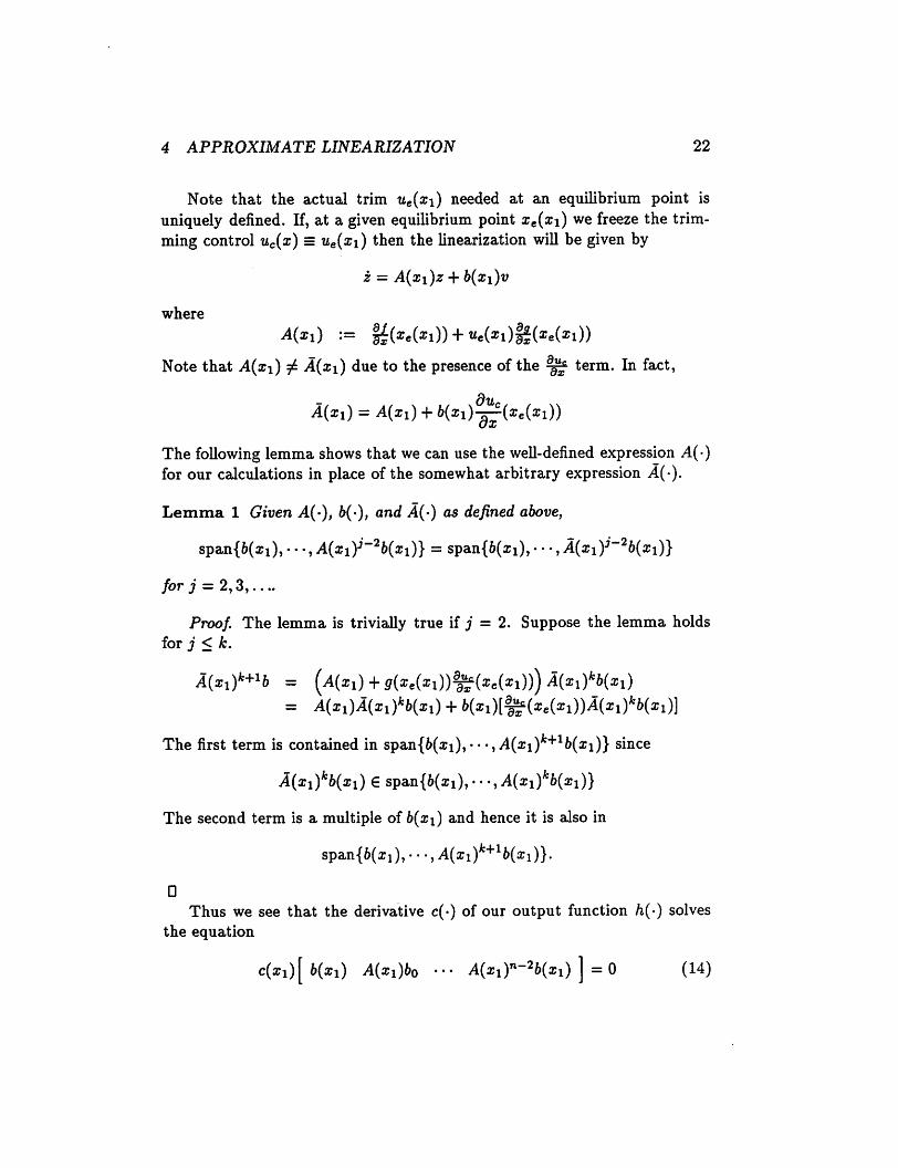
Note that the actual trim ue(xi) needed at an equilibrium point isuniquely defined. If, at a given equilibrium point xe(xi) we freeze the trimming control uc(x) = ue(xi) then the linearization will be given by

z = A(xi)z + b(x\)v

where

^(*l) '= H(*e(»l)) +««(*l)fe(*e(Xl))Note that A(xi) ^ A(xi) due to the presence of the ^ term. In fact,

— duA(xi) =A(xi) +6(xi)-^(xe(xi))

The following lemma shows that we can use the well-defined expression A(-)for our calculations in place of the somewhat arbitrary expression A(-).

Lemma 1 Given A(-), &(•), and A(-) as defined above,

span{6(xi),...,A(xi)i-26(xi)} = span{6(xi),- ••,A(xi)J"26(xi)}

/or; = 2,3,....

Proof. The lemma is trivially true if j = 2. Suppose the lemma holdsfor j < k.

A(x1)k+H = (A(xi) +5r(xe(xi))^(xe(xi)))l(xi)fc6(xi)= A(xi)A(x!)*6(xi) +6(xi)[^(xc(x1))A(xi)fc6(x1)]

The first term is contained in span{6(xi), •••, A(xi)fc+16(xi)} since

^(xi^xi) Gspan{6(xi),.-.,A(xi)/:6(xi)}

The second term is a multiple of 6(xi) and hence it is also in

span{6(xj), •••,A(xi)*+16(xi)}.

D

Thus we see that the derivative c(«) of our output function /i(-) solvesthe equation

c(x!)[&(xi) A(xi)60 ••• A(x1)n~2b(x1) ]=0 (14)


It is clear that c(xi) = (ci(xi),- -.,cn(xi)) (viewed as a differential one-form) is integrable. Indeed, we integrate

dh(x) = ci(xi)dxi H h cn(xi)dxn

to get

h(x) = / ci(xi)dxi +c2(xi)x2 +•••+cn(xi)xnFurther, since xi parameterizes the equilibrium manifold, we have the following useful fact:

Lemma 2 Suppose that c(xi) ^ 0 solves (14) with xe(xi) G £. Thenci(xi) f 0.

Proof. By Lemma 1, we may assume that f(x) = 0 for x G £• Since thesystem is linearly controllable on £, the vectors

{6(xi), A(X!)6(X!), •••, A(x1)n~2b(x1)}

are linearly independent and c(xi) lies in the left null space of these vectors.It suffices to show that e1 = (1,0, •..,0)r is linearly independent of thesevectors since this implies ci(xi) = c(xi) •e1 ^ 0. But we see that

A(Xl) •el =§f(x)Cxi Xc(xi)

and this last expression is zero since since f(x) = 0 along the equilibriummanifold, parameterized by x\. Hence e1 is in the null space of Ao and thevectors bo, Ao&o? •••, A[}~2&o are not in the null space of Ao since

{Ao&c-.^Ag^&o}are also linearly independent by the controllability assumption. Thereforee1 is linearly independent of {6o, Ao&o» •••»AJ~26o} and ci(xo) = Co •e1 ^ 0.D

Given this fact, we can write

dh(x) = ci(xi)dxi + c2(xi)dx2 + r cn(xi)dxn= <**i +gfeW +...+$fi}d*„= dxi + c2(xi)dx2 + ". + cn(xi)dxn

h(x) = Xi+c2(xi)x2H + cn(xi)xn

Any h which matches this expression to first order is also a valid outputfunction, with linear relative degree n. For the acrobot, the output functionwhich results from the above calculation is (output.m)

h(x) = xi + (6 + 4 cos Xi )x2


4.4 Approximate tracking near an equilibrium manifold

We can now extend the approximation procedure presented in Section 4.1 toconstruct a controller which tracks slowly varying trajectories near an equilibrium manifold. To do so, we extend the concept of a higher order function.We say a function is uniformly higher order on a manifold (parameterizedby xi) if it is higher order in (x2, ••-,xn). Thus in the approximation procedure, we will ignore terms which are small near the equilibrium manifold,while keeping terms that vary along the manifold. This section details thatprocedure and concludes with a proof of approximate tracking for controllaws constructed in this manner.

It will be convenient at this point to assume that /(xo) = 0 for xo G £.Although we took pains to avoid making this assumption in the previoussection, the benefit of allowing /(x0) ^ 0 is outweighed here by a tremendous increase in notation. We therefore assume that any nonlinear trim isincluded in the drift vector field. This can be accomplished in many ways,the simplist of which is to define

f(x) = f(x) - g(x)ue(xi)V = u —ue(x\)

and write our system as

x = /(x) + flf(x)vy = h(x)

Suppose the linearized relativedegree of the system (/, #) with respect toan output function h is n on an equilibrium manifold £ = {(a?i,0,•••,0)}.Assuming J(xq) = 0 for Xo G £, we define a new set of coordinates f =<t>(x) G Rn:

<f>i(x) = h(x)-ipo(x)<f>2(x) = Lj<f>i(x) - i)X(x)

<j>n(x) = Lj<j>n_i(x) - rpn-i(x)

where each if>i(x) is uniformly higher order on £. The system dynamics in f


coordinates are

ii = 6 + tfi(*) + *i(*>

tn-l = Zn +1>n-l(x) +9n_!(x)v (15)£n = i/^n(^) + ^n(a?> + V'n(^) + 0n(a;)v

y = 6 + V>o(*)

where each 0,(x) is at least uniformly first order on £. As in the previousapproximation procedure, the choice of ip allows considerable freedom inconstructing the approximation. Since the linearization is controllable on £and f|(x) satisfies (14), it follows that Lg<j>n(xo) ^ 0 for x0 G£.

Because the functions ^,- are uniformly higher order on £ and the functions 0,- are at least uniformly first order on £, the approximate system

6 = 6

in-l = fn (16)f„ = Lj<t>n(x) + Lg<j>n(x)v

y = &

is a uniform system approximation of (f,g) on 5 [4]. To provide approximatetracking control for the true system (15), we will use the exact asymptotictracking control law for the approximate system (16), namely,

1v =

Lg<f>n(x)

where

n-l

Et=0

-Lju*) +»?'(«) +E «w(yS° - *+i(»)) (17)

sn + an-1371"1 + •••+ ai5 + ao (18)

is a Hurwitz polynomial. As before, we define £d(t) to be the state trajectoryfor the approximate system induced by the desired output, &*(•),

it(0 == rf"l,WWe then expect that the tracking error

e{t) := td(t) - f(*)


will remain bounded for reasonable trajectories. In fact, we will see that thesize of the tracking error will be influenced by how far the desired trajectorystrays from the equilibrium manifold.

Since the approximate system (16) is a uniform system approximationof the true system (15) around £, we would expect that the approximationwould be valid on, for instance, a cylindrical neighborhood of £ given by

C€(€):={t:*i(e€,\\Z-*iC\\<*}

where ?rif := (fi,0, ...,0) and e is sufficiently small. We make use of thefollowing fact: it is always possible to choose £' C £ so that a given functionA(f) that is uniformly order p on £ will satisfy

ia(oi < km - Tier

for all f G Ce(£'), 0 < e < 1. For example, let A(f) = &$• Choosing£' = {i G&2 : |(i| <K,(2 = 0} will guarantee the X(() < Kg on Ce(£')»0 < € < 1.

The following theorem shows that such a control law can indeed providethe desired result and provide stable approximate tracking in the neighborhood of the equilibrium manifold.

Theorem 3 Suppose (f,g) is linearly controllable at xo and let £ be themanifold of linearly controllable equilibrium points. Further assume thatf(xe) = 0 for xe G £. Then, there exists a manifold £' C £, a changeof coordinates £ = <f>(x), and an € > 0 such that the approximate trackingcontrol law (17) results in stable approximate tracking provided £d(t) GCt(£')and \y^{t)\ < efor t > 0, and ||e(0)|| < e. Furthermore, the tracking errorwill be of order €2.

Proof. Construct a system approximation as detailed above. For convenience, define

*(0 = (^i(*).'"AW)U-i(«)*(t) = ('i(*),"-A0O)U*-i(,)

The closed loop system given by (15) and (17) can be written as

where A is a Hurwitz matrix with characteristic polynomial (18).


As discussed above, we may take £' to be such that

IWOII < *illf-*i€lla110(011 < *i||€-*rfll

||£/<M0II < Mf-nfll

for f GCs(£')j S < 1, and some ki < oo. Since Lg<f>n(x) is nonzero on £, wecan also require that £' and S be such that

< k2LgM0

for f GCs(£') and some &2 < oo. Using these bounds plus the fact that

ite-*i*ii<iwi+€

(by choice of yd(-)), it follows that there exists k^ < oo such that

IW0 + «(«HI<*3(Nla + « + €2)

where f GCs(£').Choose the Lyapunov function

V = eTPe

where P > 0 solves ATP+PA = -/. Differentiating V alongthe trajectoriesof the closed loop system, for f GCs(£') and some A?4 < oo,

V = -||e|p + 2erP(^) + 9(e)(«-«o(«)< -||e|f + *4l|e||(l|e||2 + <||e|| + £2)< -lllell2 - (| - MII'll +«))IMIa " (111*11 - *«2)2 + *?<*

If ||e|| < 25— e, we have

and hence V is strictly negative whenever 2k4€2 < \\e\\ < ^ -e. By makinge sufficiently small, we can guarantee that e(t) will converge to a ball oforder e2 for all ||e(0)|| sufficiently small. Note that the above analysis isvalid since

||£-ir10|<€ + sup||e(O||<*<l

is satisfied when e and ||e(0)|| are sufficiently small, and hence £(t) G Cs(£')under these conditions. D


Corollary 3.1 If there is a time t\ > 0 such that the desired output trajectory becomes constant, i.e., yd(t) = J/i, t > t\, then the trajectory trackingerror e(t) will converge to zero and the system will converge to the constantoperating point f = (3/1,0,..., 0).

As we mentioned above, it is possible to extend this analysis such that/(xo) = 0, xo G £ is not required. Although removing this assumptioncan unnecessarily complicate the analysis, there is one special case which isilluminating. If we choose a change of coordinates such that u never appearsin the derivatives X/+^tt<^t-, we do not need to assume that /(xo) = 0. Inthis special case we can choose

<f>i(x) = I/&_i(x) - ^,_i(x)

and no 0t_i term appears in the corresponding & since the input does notappear (by choice of V>)« It turns out that for the approximations constructedfor the acrobot, the input never appears and hence we can make use ofthis simplification and avoid the additional computational burden assocaitedwith calculations involving / = / + gu$. It is important to note that thissimplification is not generic and may fail to hold for specific systems.

The next chapter gives details on the results of applying this controllerformulation to the acrobot.

5 CONTROLLER COMPARISONS AND DISCUSSION 29

5 Controller comparisons and discussion

In this section we present comparisons of a linear and nonlinear controllersfor acrobot. We present three controllers, representing various system approximations: linearization about a point, linearization about the equilibrium manifold, and uniformly higher order approximation. In order to properly adjust for gains, we have in all cases converted the systems into (approximate) Brunowsky canonical form and then applied the appropriate designcriteria. The output function for each controller is the one derived in Section 4.3, which gives linearized relative degree n = 4 along the equilibriummanifold. Also, except as noted, we have used the special set of parametersfor acrobot which makes the equilibrium coordinates trivial. For simplicity,we refer to the controllers as linear, gain-scheduled, and nonlinear.

The linear controller was constructed by linearizing the acrobot aboutthe completely inverted position, 0X = 02 = 0 (linear.m). This configuration is roughly in the center of the operating region which we considered.The controller is implemented as a linear tracking controller (see Section 3.1)using "balancing" coordinates (i.e., the equilibrium manifold is parameterized by xi).

The gain-scheduled controller is similar to the linear controller, exceptthat all calculations are carried out as a function of xi, the projection ofthe state onto the equilibrium manifold (schedule.m). The controller isconstructed using a change of coordinates which ignores all second order andhigher nonlinearities in the variables X2,X3, X4. In that set of coordinateswe choose the gains to set the pole locations appropriately. This controlleris similar to the controllers described by [10, 12].

The nonlinear controller is constructed using a change of coordinateswhich throws away higher order terms (approximate.m) in the system velocities, X3, x4. Thus terms of the form X3 sin X2 are not thrown away in thisapproximation. Furthermore, all nonlinearities are kept in the calculationsof Lf<f>n and Lg4>n.

The gains for each controller were chosen using the same design criteria. We placed all poles of the (approximating) closed loop system at -3.5.This choice represented a compromise between performance and stability.Because the acrobot is operating in an inverted position, large overshootscan move the state out of the region of stability. Other pole locations havebeen tested, but are not presented here.

All simulations were generated using a Mathematica simulation packagethat converted system descriptions into C source and generated an exe-

5 CONTROLLER COMPARISONS AND DISCUSSION

0.15 | . 1 . r

"3 -0.05

-0.15

linear

schedula

nonlinear

0.0 1.0 2.0 3.0 4.0 5.0

time

3.0 I . 1 . 1 - 1 • r

o. 2.0

E 1.0

9 0.0

-1.0 j . L j i L

0.0 1.0 2.0 3.0 4.0 5.0

time

30

Figure 9: Stability comparison. The left plot shows the ange of the secondjoint, xi = 02. The right plot showls the angle of the center of mass of thesystem, X2 = 0i + \92.

cutable simulation program. A variable step size Runge-Kutta integratorwas used to integrate trajectories.

5.1 Stabilizing controllers

For regulation to an equilibrium point, the system performance is similar forall three controllers (stability.m). The region of attraction is not noticeably different though the linear system converges somewhat more slowly.This is due to the fact that the linear controller sees a reduced effective

gain at system configurations away from the nominal operating point. Incontrast, the nonlinear controllers provide instantaneous gain scheduling ateach position near the equilibrium manifold. This phenomenon is clearlyshown in figure 9 where the initial position was given by 0i = 0, 02 = .2 andregulation to 0i = 02 = 0 was desired.

A slice of the region of stability is shown in Figure 10. This slice showsthe set of initial conditions with 0i = 02 = 0 which converged to the origin. The region of stability is roughly uniform size about the equilibriummanifold.


Linear

Nonlinear

Figure 10: Region of attraction (0 = 0 slice)

31

Jthl


5.2 Tracking controllers

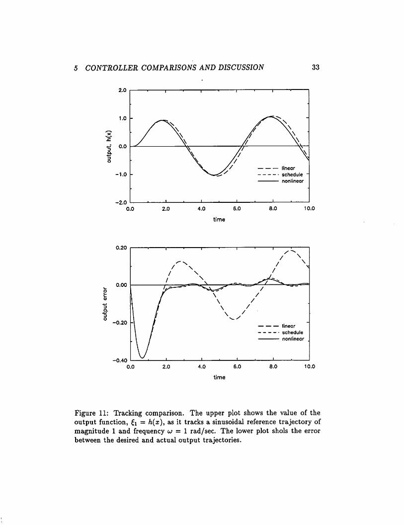
A more striking difference in controller performance is apparent when weattempt to track a trajectory (tracking.m). As evident from Figure 11,the nonlinear controllers had significantly better output tracking capability.A large part of the linear controller error results because a strictly linearcontroller cannot calculate the input necessary to hold the nonlinear system at more than one operating point (this requires a nonlinear functionor table lookup). The nonlinear controllers, however, directly provide theinstantaneous nonlinear trim needed at each different system configurationalong the equilibrium manifold.


3a.

2.0

-1.0

-2.0

0.0

0.20

0.00

-0.20

-0.40

-> r

2.0 4.0 6.0

time

8.0

linear

schedule -

nonlinear

33

10.0

linear

schedule

nonlinear

10.0

Figure 11: Tracking comparison. The upper plot shows the value of theoutput function, fi = /i(x), as it tracks a sinusoidal reference trajectory ofmagnitude 1 and frequency u = 1 rad/sec. The lower plot shols the errorbetween the desired and actual output trajectories.


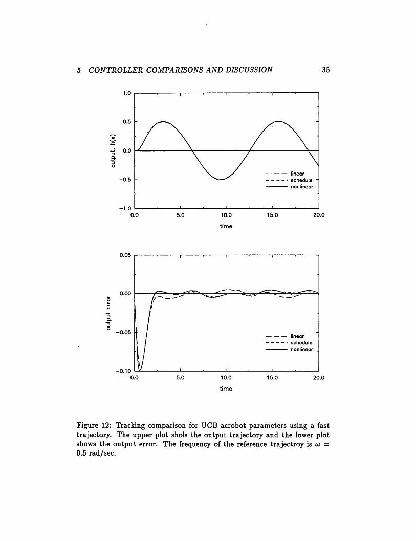
5.3 Tracking with the UCB acrobot parameters

Figure 12 shows a comparison of the three controllers using the parametervalues associated with the UC Berkeley acrobot (see Table 1). For this setof parameters, the equilibrium set has two distinct components.

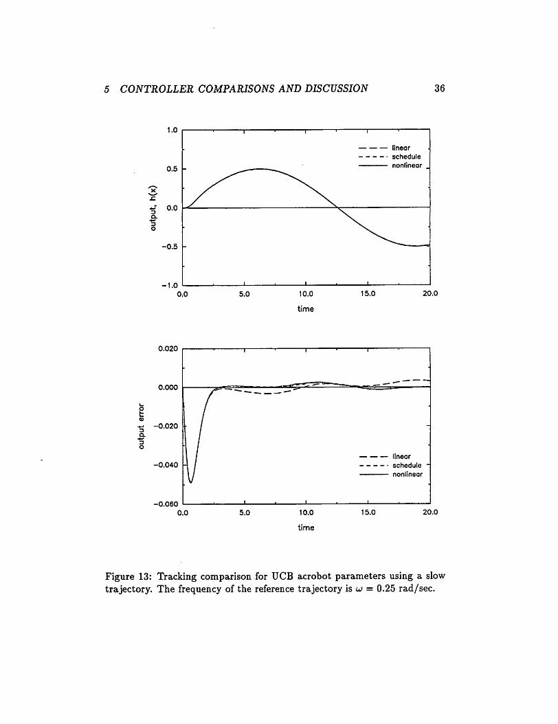
For the simulation in Figure 12 it is not clear that the nonlinear controller is improving the tracking error. However, if we slow down the desiredtrajectory, the improvement is more apparent, as shown in Figure 13. Thisimprovement is not unexpected, since one of the conditions of the Theorem 3was that the trajectory be slowly varying.


o

t93

"3Q.

3O

1.0

-0.5

-1.0

0.0

0.05

0.00

-0.05

-0.10

0.0

5.0

5.0

10.0

time

linear

schedule -

nonlinear

15.0 20.0

T ' 1 r

10.0

time

linear

schedule

nonlinear

15.0 20.0

Figure 12: Tracking comparison for UCB acrobot parameters using a fasttrajectory. The upper plot shols the output trajectory and the lower plotshows the output error. The frequency of the reference trajectroy is u —0.5 rad/sec.


o

t<o

•*-•

3a.

*->

3O

1.0

0.5 -

-0.5

-1.0

0.0

0.020

0.000

-0.020

-0.040

-0.060

0.0

5.0

5.0

T ' r

10.0

time

10.0

time

linear

schedule

nonlinear

15.0 20.0

linear

schedule -

nonlinear

15.0 20.0

Figure 13: Tracking comparison for UCB acrobot parameters using a slowtrajectory. The frequency of the reference trajectory is u —0.25 rad/sec.


5.4 Discussion

The acrobot is an example of a system which violates many of the usualassumptions which are required for defining nonlinear control laws. In particular, there is no natural output function and the system is not exactlylinearizable. This report presents a constructive technique for designingnonlinear controls for such systems. The simulations indicate that such nonlinear control laws can improve system performance, particularly trajectorytracking.

There are still many open issues to be resolved in constructing controllersfor systems such as the acrobot. Due to the freedom in choosing the systemapproximation used to construct the control law, the performance of theoverall method depends on the skill of the engineer in choosing a goodapproximation. Understanding how the choice of a given approximationaffects the controller performance would be of great benefit in improvingthe results presented here. Unfortunately, there are currently very few toolsin this area of approximation theory. Our own experiments with the acrobotindicate that intuition in this area is often misleading.

Another concern is the effect of the system approximation on the size ofthe region of stability. As mentioned in the introduction, for the acrobot it isdesirable to make the regions of stability for a controller as large as possiblein order to simplify the task of moving from the rest configuration to aninverted equilibrium point. But as the simulations of this section show (inparticular, see Figure 10), the nonlinear controllers constructed here resultin a small decrease in the region of attraction, at least in the slice of the statespace presented. Once again, tools for analyzing the regions of attractionfor a nonlinear system are not well developed.

A BALANCING COORDINATES FOR THE ACROBOT 38

Figure 14: Acrobot center of mass geometry. The center of mass is locatedon the line between the first and second link.

A Balancing coordinates for the Acrobot

In this appendix we derive the equations for the angle of the center of mass ofthe acrobot as a function of the joint angles. Figure 14 shows the geometryof the problem. The relationship between the center of mass, a, and thejoint angles is

where 6 is a function only of 92. The following identities hold for the triangle:

a = 7T - 02

C = /i

To calculate 6 given 92 we appeal first to the law of sines:

B

ffl2

sin a sin 6 sine A

A can be determined by using the law of cosines:

A2 = B2 + C2-2BCcosa

Putting all of the equations together yields the desired formula

_i 7712/2 sin 02

sin 6 =J9sina

6 = sin"

Jl\m\ +(mi + m2)2/i +2/i/2m2(mi +m2) cos02(20)

A BALANCING COORDINATES FOR THE ACROBOT 39

Figure 15: 6 versus 02 for the UC Berkeley Acrobot.

Using this equation and equation (19) gives the diffeomorphism between(0i,02)and(02,<r).

A plot of 6 as a function of 02 for the UC Berkeley Acrobot is showin Figure 15. It is clear from this picture that for 02 < 7r/2, b is wellapproximated by a simple Unear function. The slope of equation (20) at theorigin is given by

l2m2

h™>\ + (l\ + l2)m2

B Mathematica listings

This appendix contains Ustings for the Mathematica code used to analyzethe acrobot. The following files are included

acrobot .m

approximate.mattraction.m

balance.m

compare.m

equiHbrium.mexact,m

Unear.m

Unearize.m

output.m

schedule.m

stabiUty.mtracking.m

dynamic equations for the acrobotapproximate Unearizationcalculate region of attraction for control lawschange of coordinates to "balancing" coordinatesgenerate controUer comparisonsparameterization of the equiUbrium manifoldcheck involutivity conditions for feedback UnearizationUnear controller definition

Unearization calculations

construct an artificial output functiongain-scheduled controUerstabiUty simulationstracking simulations

Simulations for the acrobot were performed using a Mathematica-basedsimulation program, Simulate.m. Listings for Simulate.m are not includedhere; for further information, contact the authors.

40

c acrobot.m Fri, May 3,1991 3:17:30 pm m [email protected]

(* acrobot.m - dynamic equations for Acrobot *)Needs ["Jac"*] ;<<Trlgonometry.m (* trigonometric simplification *)

(* Unprotect the C(] function for Mathematica 1.2 *)Unprotect[C]; C = .;

(* Short function for makeing lists of rules *)SetAttributes[listRule, Listable];listRule(lhs_,rhs_] :=Rule(lhs, rhs];

(** Dynamics*

* We use the following definitions in deriving the equations of motion:*

* link 1: angle = thetal (from vertical); length = 11; mass = ml* link 2: angle = theta2 (from link 1); length = 12; mass = m2*

* a = ml 11"2 + m2 11*2

* b = m2 12*2

* c = m2 11 12

* d = g (ml 11 + m2 11)* e = g m2 12*

* Rather than let mathematica spin Its wheels on Lagrange's equtaions,* we calculate them out by hand and write the dynamics in the same form* as we usually use for robot dynamics (i.e. use mass and coriolis terms)*>

SetAttributes[{a,b,c,d,e}, Constant]SetAttributes[{ml,m2,11,12,gr), Constant)

(* define a function to substitute original parameters into an expression *)phys[x_l := x /. { a -> ml 11A2 + m2 11*2, b -> m2 12"2,

c -> m2 11 12, d -> gr (ml 11 + m2 11), e -> gr m2 12 }

(* define another function which actually uses *balanced* acrobot numbers *)balance[x_] := phys[x] /. {ll->l/2, 12->1, ml->8, m2->8, gr->10)real[x_] := phys[x] /. (ll->l/2, 12->3/4, ml->7, m2->8, gr->98/100)

(* the default set of parameters is the balanced set *)num[x_] := balance[x];Num[x_] := N[num(x]];

(* Shorthand vectors *)q := {xl, x2}w := {x3, x4)x := (xl, x2, x3, x4}

(* mass matrix and coriolis matrix *)(* use relative coords for second link *)M[q_] := {(a + b + 2 c Cos[q[[2]]], b + c Cos[q[[2]]]), {b + c Cos[q([2]]], b)}C[q_, w_] = {

{-c Sin[q[[2)]] w((2]], -c Sin[qt[2]]] (w[[l]] + w([2]])},(c Sln[q[[2]]] w[[l]], 0)

)

(* Gravity and friction *)v[q_] := d Cos(q([l]]] + e Cos[q[[lJ] + ql[2)])G(q_] := Jac[v(q), q]

(* Nonlinear vector fields *)f[q_, w_] := Join(w, -Inverse[M(q]] . (C[q,w).w + G(q))];f({xl , x2 , x3 , x4 )] = f[(xl, x2), {x3, x4)];

glq_, w_) := Joln[{0,0), Inverse(M(q]].(0, 1));g[{xl , x2 , x3 , x4 )) = g[(xl, x2), (x3, x4)];

Page 1/1 D

r~approximate.!!! Mon, Apr 8,1991 7:33:56 pm [email protected] Page 1/1 )

* Approximate linearization*

* Now we generate the change of coordinates which linearizes a* system with approximately the vector fields that we have.

*)

Print["calculating linearizing transformation"];

(* New coordinates after this transformation *)z = (zl, z2, z3, z4);

(* Rule to kill off higher order terms *)horule = {y2 y3 -> 0, y2 y4 -> 0, y3 y4 -> 0, y2A2->0, y3"2->0, y4A2->0),

phil = he;Print["phil: LeafCount(phil), " terms"];

phl2 = Together[Expand[LieDffy, phil, y]] /.Print["phi2: ", LeafCount[phi2], " terms"];

phi3 = Together[Expand[LieDffy, phi2, y]] /.Print["phi3: ", LeafCount[ph!3], " terms"];

horule];

horule];

phi4 = Together[Expand(LieD[fy, phl3, y]] /. horule);Print[nphi4: ", LeafCount[phl4], " terms"];

(* Calculate the feedback law for stabilization *)ay = Together[Expand[LieD(gy, phi4, y)] /. horule];Print["ay: ", LeafCount[ay], " terms"];

by = Together[Expand[LieD[fy, phi4, y)] /. horule);Print("by: ", LeafCount[by], " terms"];

Print("building nonlinear simulation"];

appreduce[expr_] := N[expr /.(betaOIyl) -> betaOv, betal[yl] -> betalv,beta2[yl] -> beta2v, beta3[yl] -> beta3v), 16]

BuiIdSystem[non11near,States[x];Derivs[(dxl, dx2, dx3, dx4}];Inputs[(u)];Outputs[z];Outputs[(xiId, xi2d, xi3d, xi4d)];

Local(y); (* balance and linearizing coordinates *)Local[(v)]; (* linearized input *)Local[(tl,t2)]; (* coriolis, gravity and input terms *)Local[(hl,h2,h3,h4,h5)]; (* the output function and derivatives *)Local[(betaOv, betalv, beta2v, beta3v)];

(* Default gain parameters *)Params[(Kl=150.0625, K2=171.5, K3=73.5, K4=14)];Params[(amplltude=0, offset=0, omega=l)];Paramsf(type=0)]; (* input waveform *)Params[(alphal=0.4397)); (* slope of the eq mfd *)Params[(alpha3=0.00108799)];Params[(alpha5=-0.0018839)];Include["acrotraj.c"]; (* trajectory generator *)

(* Turn off the simulation if things go crazy *)InlineC["if(fabs(xl) > 3 II fabs(x2) > 3) exit(3);"];

(* Start by converting the state to balancing coordinates *)y = num(phiB(x) /. (betaOJex] -> beta[ex], betal(ex_) -> dbeta(ex))]

(* Figure out the equilibrium mfd (beta) values *)betaOv = alphal * yl + alpha3 * Power[yl,3] + alphaS * Power[yl,5);betalv = alphal + 3 * alpha3 * yl*yl + 5 * alphaS * Power[yl,4);beta2v = 6 * alpha3 * yl + 20 * alpha5 * Power[yl,3);beta3v = 6 * alpha3 + 60 * alpha5 * Power[yl,2);

(* Now got to linearizing coordinates *)z = appreduce[(phil, phi2, phi3, phi4)];

(* Trajectory update *)InlineC("acroTrajectory((int) type, t, omega, amplitude,

offset, &hl,&h2,&h3,Sh4,&h5);");

(* apply the control law *)v - h5 - (Kl, K2, K3, K4} . (z - (hi, h2, h3, h4)) ;u = appreduce[ (-by + v) /ay);

(* Acrobot dynamics - using the equations from above *)(tl, t2) = Num[-C[q, w].w - G(q] + (0, u));(dxl, dx2) = w;(dx3, dx4) = Num[Inverse[M[q)] . (tl, t2)];

(* Store the desired and actual trajectories in transformed coords *)(xild, xi2d, xi3d, x!4d) = (hi, h2, h3, h4);

a attraction.m Tue, Sep 4,1990 9:48:04 am

(** attraction.m - figure out the region of attraction by numerical simulation*

* Richard M. Murray* June 13, 1990*

*)

VectorCheck[system_, lnterval_, vector_, min_, max_, eps_] :=Block[

(scale, good = min, bad = max, result),

For[scale = min, bad-good > eps, scale = good + (bad-good)/2,(* Simulate the system and see if it is stable *)result = Simu(system, interval, Initial->N[(scale vector))];

(* Reset good or bad depending on the result *)If [SameQ[result, ()), bad = scale, good = scale];

];good

1

VectorMax[system_, theta_) :=Block(

(x = Cos(theta), y = Sin(theta)),Print["theta = ", theta);(x, y) * VectorCheck[system, (0,10), (x,y,0,0), 0.0, 1.0, 0.01)

]

Parm[linear, amplltude->0);Parm[nonllnear, amplitude->0];LNdata = Table[VectorMax[linear, (i-1) 2 Pi / 16], (1, 1, 17}];NLdata = Table[VectorMax[nonlinear, (i-1) 2 Pi / 16], (1, 1, 17)];

graph = Show[Graphics!

(Line[NLdata), Dashing[{.02,.02)), Line[LNdata),Text("Nonlinear", Scaled((0.1,0.035)], (-1,0)],DashingUl}], Line[{Scaled[{0, 0.035)], Scaled!(0.075,0.035)) )],Text["Linear", Scaled[(0.1,0.070)], (-1,0)],Dashing[(.02, .02)], Line!(Scaled!(0,.070)), Scaled[(0.075,.070)])]),Axes->Automatic, AxesLabel->("thl", "th2"), PlotRange->All

Display["attraction.mps", graph];

[email protected] Page 1/1 )

balance.m Tue, Apr 2,1991 9:48:55 pm

(** balance.m - Change of coordinates to "balancing" coordinates*

* We now construct a change of coordinates y = phiB(x] so that the* equlibrium manifold is just (yl, 0, 0, 0).*

* This construction assumes we are using idealized coordinates. This* is also a good approximation for non-ideal coordinates (see ERL appendix)•

*)Print("calculating balancing coordinates");

y := (yl, y2, y3, y4)phiB[x List) := (x[[2]], x[[l]) + 12 m2 x[[2]) / (11 ml + (11 + 12) m2),

x[[4]], x[[3]] + 12 m2 x[[4]] / (11 ml + (11 + 12) m2)}ihpB[y List] := (y[[2]] - 12 m2 y([l]) / (11 ml + (11 + 12) m2), y[[l]],

y[[4]] - 12 m2 y[[3]] / (11 ml + (11 + 12) m2), y[(3)])

(* Push the vector fields through the change of coordinates *)(* This is slightly simplified since the coordinate change is linear *)fBy = Together! Jac[phiB[x], x] . f[ihpB[y]) ];gBy = Together! Jac[phiBtx], x] . g[ihpB[y]) ];

(* Figure out what the equilibrium input must be in order to balance *)(* See equilibrium.m for comments *)eqrule = listRule[Last[y], 0);ue = (u -> num[ -m2 12 gr Sin(xl+x2] /. listRule(x, ihpB(y]] /. eqrule]);

[email protected] Page 1/1 3

c compare.m Frl, May 3,1991 9:45:24 am

(•* compare.m - generate plots for the controller comparisons chapter*

* Richard M. Murray* August 31, 1990*

* All simulations generated by this file use the *real* values of acrobot* instead of the ideal values. (RMM 4/2/91)

*)

(* Read in the basic description of acrobot *)<<acrobot.m

(* Express vector fields in equilibrium coordinates *)(* Use special routine optimized for balanced parameters *)<<balance.m

(* Use a linear approximation to the equlibrium manifold *)(*Clear[alphal] (* alphal = eq mfd slope (keep symbolic) *)Print["using approximate balancing coordinates"]<< appbalance.m« appoutput.m (* read a save output function *)*)

(* Generate the output function used by all controllers *)« output.mhe = FindOutput[fBy, gBy, ue, y]

(* Desired trajectory; set amplitude = 0 for setpolnt tracking *)desired = amplitude Sin[omega t] + offset;SetAttributes[(amplitude,offset, omega). Constant);

(* Build the individual systems *)« Simulate.m

« linear.m

« schedule.m

<< approximate.m

Print("Using lsoda integrator")Map[SetOptions[#, Method->lsoda)fi, (linear,schedule,nonlinear)]

(* Mathematica generated plots *)(* Run this manually; It takes a while to finish *)(* « linearize.m *)

(* Now run the simulations for each part of the chapter *)(* These should be run manually since they take a while *)(* « stability.m *) (* set point stability *){* « attraction.m *) (* region of attraction *)(* « tracking.m *) (* tracking comparisons *)(* « poles.m *) (* effect of moving poles *)

[email protected] Page 1/1 D

c equilibrium.m Tue, Apr 2,1991 9:45:04 pm

(** Change of coordinates to "balancing" coordinates*

* We now construct a change of coordinates y = phiB[x] so that the* equllbrium manifold is just (yl, 0, 0, 0). This construction holds* for general parameter values.*

*)Print("calculating balancing coordinates"];

y := (yl, y2, y3, y4)phiB[x List] :=

Block"((* Use the law of cosines to get the inner angle *)(thl, th2, beta),beta = -ArcSln[ Sin[th2) /Sqrt[l + (ml+m2)A2 11A2 / (12 m2)A2 + 2(ml+m2)ll Cos(th2] / (12 m2)] ];

(* Now figure out the coordinates + velocities *)(x((2]], thl-beta, x[[4]], Jac[thl-beta, (thl, th2)) . x[[(3,4}]]} /.(thl->x[[l]], th2->x[[2]]}

)

ihpB[y List] :=Block"!

(* Use the law of cosines to get the inner angle *)(sig, th2, beta),beta = -ArcSint Sin(th2) /

Sqrt[l + (ml+m2)A2 11"2 I (12 m2)A2 + 2(ml+m2)ll Cos[th2] / (12 m2)] ];

(* Now figure out the coordinates + velocities *)(y[[2)]+beta, y[[l]], Jac[sig+beta, (th2, sig}) . y(((3,4}]], y[[3])} /.(th2->y[[l]], sig->y[[2]]}

]

(* Push the vector fields through the change of coordinates *)acroSimplify[e_] := Together[Expand[num[e]]]fBy = acroSimplify[(Jac[phiB[x), x) . f[x]) /. listRule[x, ihpB[y]]J;gBy = acroSimplify[ (Jac[phiB[x), x] . g(x]) /. listRule.Ix, ihpB[yl]];

(** Figure out what the equilibrium input must be in order to balance*

* This used to be a linear equation, but the general acrobot doesn't* support that. Fortunately, we can write down the solution in closed* form In the original set of coordinates.*

* Old code:

* solns = Solve((fy + gy u //. eqrule) == 0, u];* If[Length(solns] != 1,* Print["Can't solve equations for equilibrium input\n"]; ue = 0,* ue = solns![1]]];*

*)eqrule = UstRulelLast (y), 0];ue = (u -> num( -m2 12 gr Sin[xl+x2] /. listRule[x, ihpBty]] /. eqrule]};

[email protected] Page1/1 I

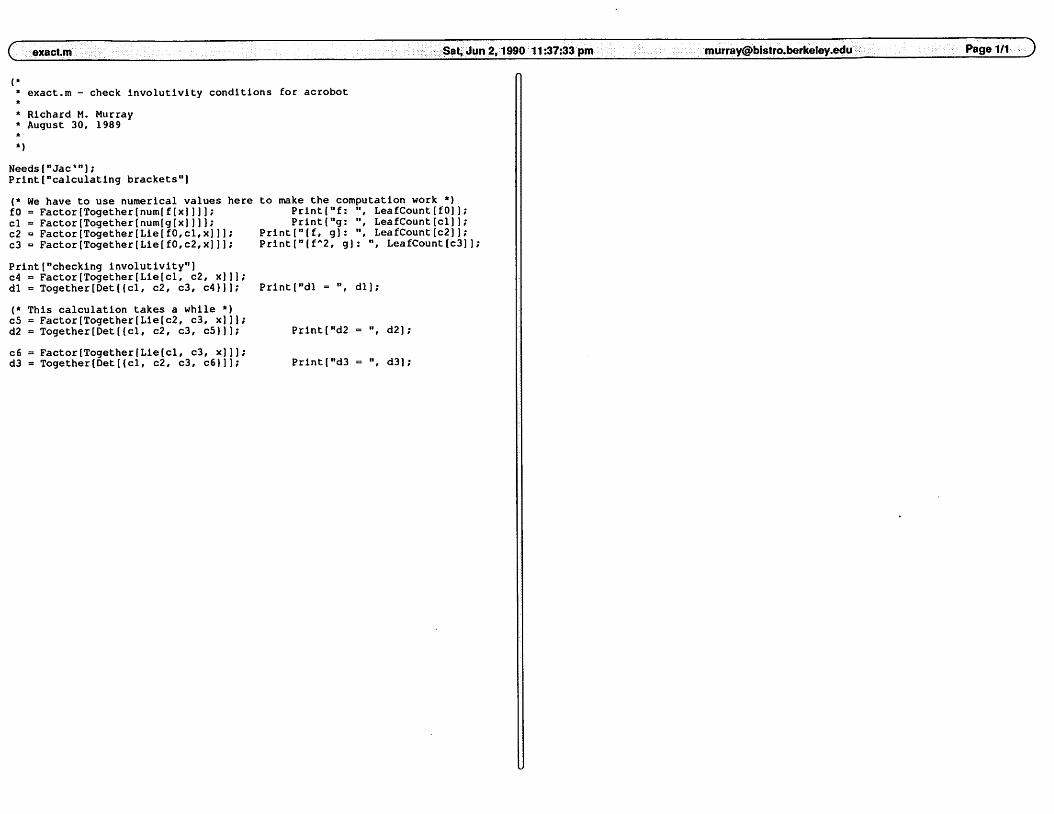
c exact.m

* exact.m - check involutlvity conditions for acrobot*

* Richard M. Murray* August 30, 1989

Sat, Jun 2,1990 11:37:33 pm

Needs("Jac%");Print("calculating brackets")

(* We have to use numerical values here to make the computation work *)fO = Factor[Together[num[f(x)])]; Print["f: ", LeafCount[fO]);cl = Factor[Together[num[g[x) ]] ]; Prlntfg: ", LeafCount[cl)];c2 = Factor[Together[Lie[fO,cl,x])]; Print["(f, g): ", LeafCount[c2]];c3 = Factor[Together[Lie[fO,c2,x])]; Print["(fA2, g] : ", LeafCount[c3]]

Print("checking involutlvity")c4 = Factor[Together[Lie[cl, c2, x])];dl = Together[Det((cl, c2, c3, c4})];

(* This calculation takes a while *)c5 = Factor[Together(Lie[c2, c3, x]]);d2 = Together[Det[(cl, c2, c3, c5))];

c6 = Factor(Together[Lie[cl, c3, x]]];d3 = Together[Det[(cl, c2, c3, c6)]];

Print("dl = dl];

Print("d2 = ", d2];

Print("d3 = ", d3];


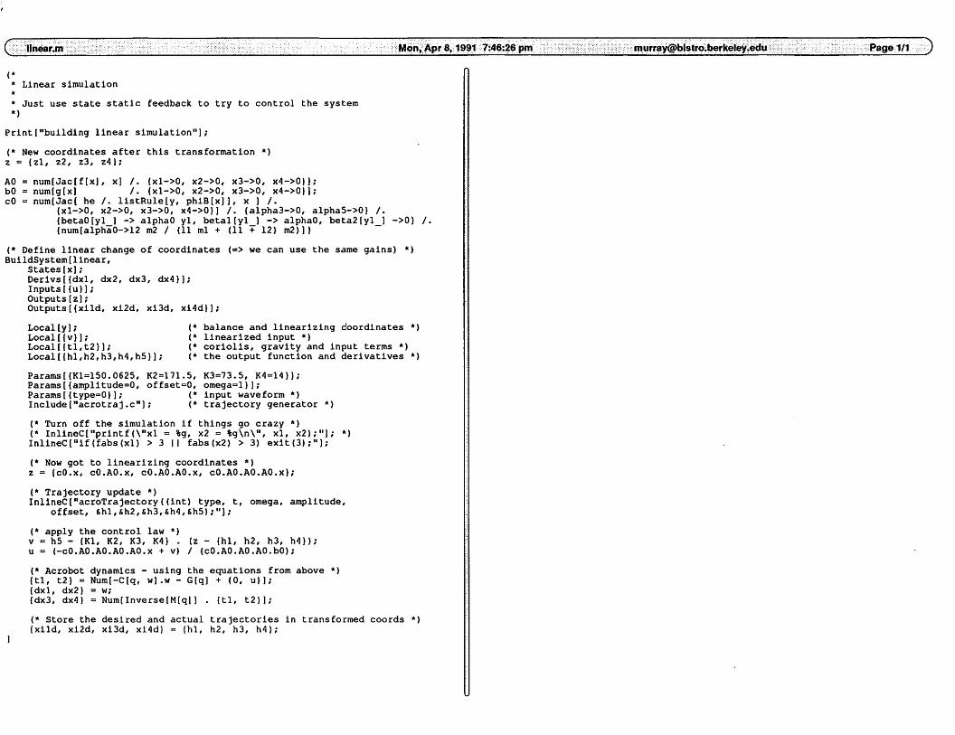
c linearjn Mon, Apr 8,1991 7:46:26 pm

(** Linear simulation*

* Just use state static feedback to try to control the system

*)

Print["building linear simulation"];


AO = num(Jac[f[x], x] /. (xl->0, x2->0, x3->0, x4->0}];bO = num[g(x) /. (xl->0, x2->0, x3->0, x4->0)];cO = num[Jac( he /. listRule[y, phiB[x]], x ) /.

(xl->0, x2->0, x3->0, x4->0}] /. (alpha3->0, alpha5->0} /.(betaO[yl_) -> alphaO yl, betal[yl_] -> alphaO, beta2(yl_] ->0} /.(num[alphaO->12 m2 / (11 ml + (11 + 12) m2)]}

(* Define linear change of coordinates (=> we can use the same gains) *)BuildSystem[linear,

States[x];Derivs[(dxl, dx2, dx3, dx4});Inputs[(u)];Outputs[z];Outputs[{xiId, xi2d, xi3d, xi4d}];

Local[y];Local[(v}];Local[{tl,t2}];Local[(hi,h2,h3,h4,h5}];

(* balance and linearizing coordinates *)(* linearized input *)(* coriolis, gravity and input terms *)(* the output function and derivatives *)

Params[(Kl=150.0625, K2=171.5, K3=73.5, K4=14}];Params[(amplltude=0, offset=0, omega=l}];Paramsf(type=0)]; (* input waveform *)Include("acrotraj.c"); (* trajectory generator *)

(* Turn off the simulation if things go crazy *)(* InlineC["printf(\"xl = %g, x2 = %g\n\", xl, x2);"]; *)InlineC["if(fabs(xl) > 3 || fabs(x2) > 3) exit(3);"];

(* Now got to linearizing coordinates *)z = (cO.x, cO.AO.x, cO.AO.AO.x, cO.AO.AO.AO.x);

(* Trajectory update *)InlineCfacroTrajectory ((int) type, t, omega, amplitude,

offset, Shl,Sh2,&h3,&h4,«h5);");

(* apply the control law *)v = h5 - (Kl, K2, K3, K4) . (z - (hi, h2, h3, h4}>;u = (-cO.AO.AO.AO.AO.x + v) / (cO.AO.AO.AO.bO);

(* Acrobot dynamics - using the equations from above *)(tl, t2) = Num[-C[q, w].w - G[q] + (0, u}];(dxl dx2) = w;(dx3! dx4) = Num[Inverse[M(ql] . (tl, t2}];

(* Store the desired and actual trajectories in transformed coords *)(xild, xi2d, xi3d, xi4d} = (hi, h2, h3, h4);

[email protected] Page 1/1 J

G linearize.m Thu, May 2,1991 5:32:35 pm

(** linearize.m - check out the linearization of acrobot*

* Richard M. Murray* June 2, 1990*

*)

(* Figure figure out the linearization about the vertical equilibrium point *)AO = num[Jac(f[x], x] /. (xl->0, x2->0, x3->0, x4->0}];bO = num[g[x] /. (xl->0, x2->0, x3->0, x4->0}];

(* Controllable ??*)Print("Linear controllability = ", Det[(bO, AO.bO, AO.AO.bO, AO.AO.AO.bO))];

(* Now figure out the points at which we loose controllability *)uA = real[Jac[f[x], x] /. (xl->-x2/2, x3->0, x4->0});uB = real[g(x] /. (xl->-x2/2, x3->0, x4->0}];

bA = balance(Jac[f[x], x] /. (xl->-x2/2, x3->0, x4->0}];bB = balance(g[x) /. (xl->-x2/2, x3->0, x4->0}];

balDet(v_] :=Det[Map[N[# /. x2->v]fi, (bB, bA.bB, bA.bA.bB, bA.bA.bA.bB}]);

balSigma[v_] :=SingularValues[

Map[N(# /. x2->v]fi, (bB, bA.bB, bA.bA.bB, bA.bA.bA.bB)])!(2]];

ucbDet(v_) :=Det[Map(N[# /. x2->v]fi, (uB, uA.uB, uA.uA.uB, uA.uA.uA.uB))) ;

ucbSigma[v_] :=SingularValues[N[(uB, uA.uB, uA.uA.uB, uA.uA.uA.uB) /. x2->v]][(2)];

ucbGraph = Plot[ucbDet[x2], (x2, -Pi, Pi}]Display("ucbctrl.mps", ucbGraph]

balGraph = Plot[balDet[x2], (x2, -Pi, Pi}]Display["balctrl.mps", balGraph]

[email protected] Page1/1 j>

putputm Fri, Aug 31,1990 9:22:13 am

* Determination of the output function*

* We now calculate the output function by using the linearization along* the equilibrium manifold (y2 = y3 = y4 =0). This makes use of* a special set of parameters to simplify calculations, so from here* on out, all of the calculations are numerical.*

*)

FindOutput[fBy_, gBy_, ue_, y_] :=Block[

(Ae, be, ce, W, 1),Print("determining output function"];

(* Get the vector fields and evaluate them *)(*! These are required by functions outside of this one !*)fy = num[fBy];gy = num[gBy];

(* Make a rule to evaluate an expression at an equilibrium point *)eqrule = listRule[Rest[y], 0];

(* Now figure out what the linearization is along the eq manifold *)Print[" calculating linearization along eq manifold");Ae = Jac[fy + gy u, y) /. ue //. eqrule;be = gy //. eqrule;

(** Originally we calculated the output function by using the controllable* canonical form of the linearized system. Now we know better, so we* just look at the null space of the controllability matrix*

*)Print[" null space calculation"];W = (be);For[i = 2, 1 < Length[be], ++1, W = Join[W, (Ae.Last[W]))];ce = Together! NullSpacelW][[1]] ];

(* Return the normalized output function *)Together! ce/ce((l)] ] . y


( schedule.m Wed, May 22,1991 11:03:00 am [email protected] Page 1/1

(** Gain scheduling*

* Now we generate the change of coordinates which linearizes a* system with approximately the vector fields that we have.*

*)

Print("calculating linearizing transformation"];


(* Rule to kill off higher order terms *)horule = (y2 y3 -> 0, y2 y4 -> 0, y3 y4 -> 0, y2A2->0, y3A2->0, y4A2->0);

normal[expr_SeriesData] := Normal(expr);normal[expr_] := expr;

expand[expr_] := Expand[normal[Series[expr, (y2,0,l)]]]reduce[expr_] := Together[expand[expr] /.horule //. (Hold[Normal[aj]->a)];

(* Build the transformation; use Taylor series to get linear truncation *)phil = reduce[he];Print["phil: ", LeafCount[phil], " terms"];

phi2 = reduce[LieD[fy, phil, y]]Print["ph!2: ", LeafCount[ph!2], terms"];

phl3 = reduce[LieD[fy, phi2, y])Print("phi3: ", LeafCount[phi3], " terms"];

phi4 = reduce[LieD(fy, phi3, y)]Print("phi4: ", LeafCount[phi4), " terms"];

(* Calculate the feedback law for stabilization *)(* Truncate the linear terms *)ay = reduce(LieD(gy, phi4, yj);Print["ay: ", LeafCount[ay], " terms");

by = reduce[LieD(fy, phl4, y]);Print["by: ", LeafCount(by), " terms"];

Print["building schedule simulation"];

BuildSystem(schedule,States[x];Derivs[(dxl, dx2, dx3, dx4}];Inputs!(u)];Outputs[z];Outputs I(xild, xi2d, xi3d, xi4d}];

Local[y]; (* balance and linearizing coordinates *)LocalI(v)J; (* linearized input *)Local[(tl,t2)]; (* coriolis, gravity and input terms *)Local[(hi,h2,h3,h4,h5}]; (* the output function and derivatives *)Local((betaOv, betalv, beta2v, beta3v});

(* Default gain parameters *)Params((Kl=150.0625, K2=171.5, K3=73.5, K4=14}];Params((amplitude=0, offset=0, omega=l});Params[(type=0)); (* input waveform *)Params((alphal=0.4397}] ; (* slope of the eq mfd *)Params[(alpha3=0. 001087 99));Params[(alpha5=-0.0018839)} ;

Include("acrotraj.c"); (* trajectory generator *)

(* Turn off the simulation if things go crazy *)InlineC["if(fabs(xl) > 3 II fabs(x2) > 3) exit(3);"];

(* Start by converting the state to balancing coordinates *)y = num(phiB[x) /. (beta0[ex_] -> beta(ex], betal[ex] -> dbeta[ex]});

(* Figure out the equilibrium mfd (beta) values *)betaOv = alphal * yl + alpha3 * Power[yl,3] + alpha5 * Power[yl,5];betalv = alphal + 3 * alpha3 * yl*yl + 5 * alpha5 * Power[yl,4];beta2v = 6 * alpha3 * yl + 20 * alphaS * Power[y1,3];beta3v = 6 * alpha3 + 60 * alpha5 * Power[yl,2];

(* Now got to linearizing coordinates *)z = (phil, phi2, phi3, phi4);

(* Trajectory update *)InlineC("acroTrajectory((int) type, t, omega, amplitude,

offset, Shl,fih2,fih3,sh4,sh5);"];

(* apply the control law *)v = h5 - (Kl, K2, K3, K4} . (z - (hi, h2, h3, h4}) ;u = (-by + v) / ay;

(* Acrobot dynamics - using the equations from above *)(tl, t2} = Num[-C(q, w].w - G[q] + (0, u}];(dxl, dx2} = w;(dx3, dx4} = Num(Inverse[M[q)] . (tl, t2}];

(* Store the desired and actual trajectories in transformed coords *)(xild, xi2d, xi3d, xi4d) = (hi, h2, h3, h4);

( tracking.m Fri, May 3,1991 10:05:57 am

(* Tracking simulations *)Parm[schedule, amplitude->l, offset->0, omega->l, type->0]Simu[schedule, (0, 20, .02}, Output->"tracking.sch", Initial->(0, 0, 0, 0)]

Parm[nonlinear, amplitude->l, offset->0, omega->l, type->0]Simu [nonlinear, (0, 20, .02), Output->"tracking.nlc", Inltial->(0, 0, 0, 0)]

Parm[linear,Simu[linear,

amplitude->l, offset->0, omega->l, type->0](0, 20, .02), Output->"tracking.lin", Initial->(0, 0, 0, 0)]

[email protected] Page 1/1 )

i stability.m Fri, May 3,1991 9:53:40 am

(* Simulate the system with some various starting points *)Parm(nonlinear, Kl->150.0625, K2->171.5, K3->73.5, K4->14]Parmjnonlinear, amplitude->0, offset->0)(*Simu[nonlinear, (0, 10), Output->"nonlinear.l", Initial->(0, 0.01, 0, 0}]Simu[nonlinear, (0, 10), 0utput->"nonlinear.2", Initial->(0.01, 0, 0, 0)]Simu[nonlinear, (0, 10), 0utput->"nonlinear.3", Initial->{-0.02, 0.03, 0, 0)]Simu[nonlinear, (0, 10), Output->"nonlinear.4", Initial->(0.1, 0, 0, 0}]MSimu[nonlinear, (0, 5, .02), Output->"stabllity.non", Initial->(0, 0.2, 0, 0}]

(* Simulate the system with some various starting points *)Parm(schedule, Kl->150.0625, K2->171.5, K3->73.5, K4->14]Parm[schedule,

(*Simu(schedule,Simu[schedule,Simu[schedule,Simu(schedule,

*)Simu[schedule, (0, 5, .02), Output->"stability.sch", Initial->{0, 0.2, 0, 0})

amplitude->0, offset->0]

(0, 10), Output->"schedule.l",(0, 10), Output->"schedule.2",(0, 10), Output->"schedule.3",(0, 10), Output->"schedule.4",

Initial->{0, 0.01, 0, 0))Initial->{0.01, 0, 0, 0}]Initial->{-0.02, 0.03, 0,Inltial->{0.1, 0, 0, 0}]

(* Simulate the system with some various starting pointsParm[linear, Kl->150.0625, K2->171.5, K3->73.5, K4->14]

amplitude->0, offset->0]

10), Output->"linear.l",10}, Output->"linear.2",10}, Output->"linear.3",10}, Output->"linear.4",

')

Initial->(0, 0.01,Initial->(0.01, 0,Initial->(-0.02, 0Initial->{0.1, 0,

0, 0)]0, 0)]03, 0,

0, 0)]0}]

0}]

Parm[linear,

l

Simu[linear,Simu[linear,Simu(linear,Simu[linear,

*)Simu(linear,

(0,(0,(0,(0,

(0, 5, .02), Output->"stabillty.lln", Initial->{0, 0.2, 0, 0}]

Null


REFERENCES 42

[13] S. Wolfram. Mathematica: A System for Doing Mathematics by Computer. Addison-Wesley, 1989.

REFERENCES 41

References

1] W. T. Baumann and W. J. Rugh. Feedback control of nonlinear systemsby extended linearization. IEEE AC Transactions, 31:40-46, 1986.

2] C. I. Byrnes and A. Isidori. Local stabilization of minimum-phase nonlinear systems. Systems and Control Letters, 11:9-17, 1988.

3] J. Hauser, S. Sastry, and P. Kokotovic. Nonlinear control via approximate input-output linearization, the ball and beam example. TechnicalReport ERL, Department of EECS, University of California, Berkeley,1989. To appear in IEEE Transactions on Automatic Control, 1991.

4] John Hauser. Nonlinear control via uniform nonlinear system approximation. In IEEE Control and Decision Conference, 1990. To appearin Systems and Control Letters, 1991.

5] L. R. Hunt, R. Su, and G. Meyer. Global transformations of nonlinearsystems. IEEE AC Transactions, AC-28(1):24-31, 1983.

6] A. Isidori. Nonlinear Control Systems. Springer-Verlag, 2nd edition,1989.

7] B. Jakubczyk and W. Respondek. On linearization of control systems. Bulletin de L'Academie Polonaise des Sciences, Serie des sciences mathematiques, XXVIIL517-522, 1980.

8] A. J. Krener. Approximate linearization by state feedback and coordinate change. Systems and Control Letters, 5:181-185,1984.

9] A. J. Krener, S. Karahan, M. Hubbard, and R. Frezza. Higher orderlinear approximations to nonlinear control systems. In IEEE Controland Decision Conference, pages 519-523, 1987.

[10] C. Reboulet and C. Champetier. A new method for linearizing nonlinear systems: the pseudolinearization. International Journal of Control, 40:631-638, 1984.

[11] M. W. Spong and M. Vidyasagar. Dynamics and Control of RobotManipulators. John Wiley, 1989.

[12] J. Wang and W. J. Rugh. On the pseudo-linearization problem fornonlinear systems. Systems and Control Letters, 12:161-167, 1989.

copyright © 1991, bythe author(s). all rights reserved

Documents