Copepod's 2 lens telescope

Trilobite fossil 500 million years

Black antHouse Fly

Scallop

Octopus

Cuttlefish

Eyes everywhere…

Modeling fly phototransduction:how quantitative can one get?

Limits of modeling?

• vertebrate phototransduction (rods, cones)

• insect phototransduction

• olfaction, taste, etc…

Comparative systems biology?

Fly photo-transduction

• About the phenomenon

• Molecular mechanism

• Phenomenological Model

• Predictions and comparisons with experiment.

Outline:

Compound eyeof the fly

Fly photoreceptor cell

hv

50nm

1.5 m

Na+, Ca2+

Microvillus

Rhodopsin

Single photon response in Drosophila: a Quantum Bump

Lowlight

Dimflash

“All-or-none” response

Henderson and Hardie, J.Physiol. (2000) 524, 179

Comparison of a fly with a toad.

From Hardie and Raghu, Nature 413, (2001)

Single photon response:

Notedifferent scales directions of current!!

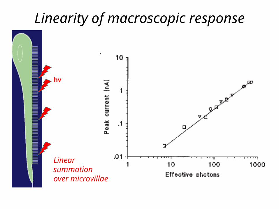
Linearity of macroscopic response

hv

Linearsummationover microvillae

Average QB wave-form

A miracle fit:

Henderson and Hardie, J.Physiol. (2000) 524, 179

QB aligned at tmax

QB variability

Peak current Jmax (pA)#

even

ts

rms J

mean J

( )

( ).4max

max

0

# of

eve

nts

Latency (ms)

Latency distribution

Multi-photon response

QB waveform

Convolutionwith latencydistribution

Macroscopic response = average QB

Latency distributiondetermines the averagemacroscopic response

!!! Fluctuations control the mean !!!

Advantages of Drosophila photo-transduction as a model

signaling system:

• Input: Photons• Output: Changes in membrane potential• Single receptor cell preps• Drosophila genetics

Molecular mechanism offly phototransduction

Response initiation

IP3 + DAG PIP2

PKCG

GDP PLCTrp

High [Na+], [Ca++]

Low [Na+], [Ca++]

Ca pump

*GTP

GDP

G

GTP Trp*

Na+, Ca++

DAG

Cast: Rh = Rhodopsin; GG-protein

PIP2 = phosphatidyl inositol-bi-phosphateDAG = diacyl glycerol

PLC = Phospholipase C -beta ; TRP = Transient Receptor Potential Channel

DAG Kinase

Rh

hv

*Rh*

Positive Feedback

PKC

Na+, Ca++

PLC

PIP2 IP3 + DAG

hv

*GGDP GTP

GDP

G

GTP Trp

Rh

High [Ca++]

Intermediate [Ca++]

DAG

Trp*

**

Intermediate [Ca] facilitates opening of Trp channelsand accelerates Ca influx.

Ca pump

Negative feedback and inactivation

PKC

Na+, Ca++

PLC

PIP2 IP3 + DAG

*GGDP GTP

GDP

G

GTP

Rh*

High [Ca++]

**

Cast: Ca++ acting directly and indirectly e.g. via PKC = Protein Kinase Cand Cam = Calmodulin

Arr = Arrestin (inactivates Rh* )

High [Ca++]

**Cam ??

Arr

Ca pump

Trp*

Comparison of early steps

From Hardie and Raghu, Nature 413, (2001)

Vertebrate Drosophila

2nd messengers

cGMPDAG

…and another cartoonc.

d

a.

b.

From Hardie and Raghu, Nature 413, (2001)

InaD signaling complex

InaDPDZ domainscaffold

From Hardie and Raghu, Nature 413, (2001)

Speed and space: the issue of localization and confinement.

Order of magnitude estimate of activation rates:

G* ~ PLC* ~ k [G] ~ 10m2/s 100 / .3 m2 > 1 ms-1

Diffusion limit onreaction rate

Protein (areal) density

! FastEnough !

Possible role for InaD scaffold !

However if: ~ 1m2/s 10 / .3 m2 =.03ms-1 << 1 ms-1

! Too Slow !

How “complex” should the model

of a complex network be?

A naïve model

“Input” TRP channel Ca2+

( G*, PLC*, DAG)

low

high

Kinetic equations:Activation stage ( G-protein; PLC; DAG ):

d

dtA A IA 1

QB “generator” stage ( Trp, Ca++ ):

d

dtTrp A F Ca Trp F Ca Trp

d

dtCa Trp Ca Ca Ca Ca

nTrp

ex Ca

* ( ) ( ) *

[ ] *([ ] [ ]) ([ ] [ ])

*

1

10

# open channels Positive and negative feedback

Ca++ influx via Trp* Ca++ outflow/pump

Input (Rh activity)

Feedback Parameterization

F Ca gCa K

Ca KD

m

Dm

( )

([ ] / )

([ ] / )

1

1

Parameterized by the “strength” g(~ ratio at high/low [Ca])

Characteristic concentration KD

and Hill constant m

Note: this has assumed that feedback in instantaneous…

Null-clines and fixed points

0 100 200 300 400 5000

0.1

0.2

0.3

0.4

0.5

0.6

0.7

A=.2

.05

.03

A=.02

[Ca]/[Ca0]

Trp

*/T

rp

[Ca]=0

[TRP*]=0null-cline

Problems with the simple model

Model Experiment

• In response to a step of Rh* activity (e.g. in Arr mutant ) QB current relaxes to zero

• Ca dynamics is fast rather than slow no “overshoot”

• Long latency is observed

“High”

fixed point

Order of magnitude estimate of Ca fluxes

[Ca]dark ~ .2M

[Ca]peak ~ 200M

1 Ca ion / microvillus

1000 Ca ion / microvillus

30% of 10pA Influx 104 Ca2+ / ms

Hence, Ca is being pumped out very fast ~ 10 ms-1

[Ca] is in a quasi-equilibrium

Note: villus volume ~ 5*10-12 l

Microvillus as a Ca compartment

Compare 10 ms-1 with diffusion rate across the microvillus:

-1 ~ Dca / d2 ~ 1 m2/ms / .0025 m2 = 400 ms -1

But diffusion along the microvillus:

-1 ~ 1 m2/ms / 1 m2 = 1 ms -1 is too slowcompared to 10ms-

1

50nm

1-2 um

Hence it is decoupled from the cell.

Note: microvillae could not be > .3m in diameter,i.e it is possible the diameter is set by diffusion limit

Ca++

Slow negative feedback

Assume negative feedback is mediated

by a Ca-binding protein (e.g. Calmodulin??)

d

dtB k Ca B Bx x

* *[ ] 1

F B gB K

B KD

m

Dm

( *)

([ *] / )

([ *] / )1

1

Slow relaxation

A more ‘biochemically correct’ model:d

dtG* ...

d

dtPLC* ...

d

dtDAG[ ] ...

d

dtTrp* ...

d

dtCa[ ] ...

d

dtB[ *] ... Delayed

Ca negative feedback

F+

F-

Feedback

Cascaded

dtRh* ...

Stochastic effects

Gillespie, 1976, J. Comp. Phys. 22, 403-434see also Bort,Kalos and Lebowitz, 1975, J. Comp. Phys. 17, 10-18

Numbers of active molecules are small !e.g. 1 Rh*, 1-10 G* & PLC*, 10-20 Trp*

Chemical kinetics

Master equation

Numerical simulation

Reaction “shot” noise.

Stochastic simulationEvent driven Monte-Carlo simulationa.k.a. Gillespie algorithm

Gillespie, 1976, J. Comp. Phys. 22, 403-434see also Bort,Kalos and Lebowitz, 1975, J. Comp. Phys. 17, 10-18

Numbers of molecules (of each flavor) #Xa(t) are updated

#Xa(t) #Xa(t) +/- 1 at times ta,i

distributed according to independent Poisson processes

with transition rates a,. Simulation picks the

next “event” among all possible reactions.Note: simulation becomes very slow if some of the Reactions are much faster then others. Use a “hybrid” method.

The model is phenomenological…

Many (most?) details are unknown:

e.g. Trp activation may not be directly by DAG, but via its breakdown products; Molecular details of Ca-dependent feedback(s) are not known; etc, etc

there’s much to be explained on a qualitative andquantitative level…

BUT

Identifying “submodules”d

dtG* ...

d

dtPLC* ...

d

dtDAG[ ] ...

d

dtTrp* ...

d

dtCa[ ] ...

d

dtB[ *] ... Delayed

Ca negative feedback

F+

F-

Feedback

Cascaded

dtRh* ...

Keydynamicalvariablesdefine“Submodules”

Rephrased in a “Modular” form: the “ABC model”

“Input” Channel

B

( Rh*, G*)

Activator

(PLC, Dag)

(TRP)

(Ca-dependent inhibition)

Ca++

Ca++

Activator – Buffer – Ca-channel

Quantum Bump generation

0 200 400 600 800 10000

5

10

15

20

25

20

60

100

140

180

200 4000 600

TRP*

B*/10PLC*

A

Threshold for QB generation

A

B*

(A,B) - “phase” plane

High probabilityof TRP channelopening

“INTEGRATE & FIRE”process

What about null-cline analysis?Problems:

• 3 variables A,B,C• Stochasticity

• Discreteness

C

B1 2 3 40

“Ghost”fixed point

dX

dtx x x x 0 1 1 Prob ( Prob () )

Generalized “Stochastic Null-cline”

Can one calculate anything?

E.g. estimate the threshold for QB generation:

A-1 A A+1

C = 0 1 2

PLC* PLC*

Am Am f([Ca])Positive feedbackkicks in once channels open

Threshold A = AT such that

Prob (AT -> AT +1) = Prob (C=0 -> C=1)

NOTE: Better still to formulate as a “first passage” problem

Condition for QB generation

PLC*

[Ca]

1

2

3

4

0

[Ca]

A

Prob (C=1 C=2) > Prob (C=1 C=0)

Amax~ PLC*

*AT

AT > AQB ([Ca])

AQB ([Ca])

Bistable region/Bimodal response

Reliable QBgeneration

Quantum Bump theory versus reality

Model ExperimentLatencyhistogram

Average QBprofile

Fitting the data: QB wave-formT

rp*/

Trp

tot

Time (arbs)

There is a manifoldof parameter valuesproviding good fitfor < QB > shape !!

So what ???“With 4 parameters I canfit an elephant and with 5 it will wiggle its trunk.” E. Wigner

Non-trivial “architectural” constraints

Despite multiplicity of fits, certain constraints emerge:

• Trp activation must be cooperative• Activator intermediate must be relatively stable: “integrate and fire” regime.• Negative feedback must be delayed• Multiple feedback loops are needed

Etc, …Furthermore:

Fitting certain relation between parameters: “phenotypic manifold” - the manifold in parameter space corresponding to the same quantitative phenotype.

Many more features to explain quantitatively!

Constraining the parameter regime…

Help from the data on G-protein hypomorph flies:

• # of G-proteins reduced by ~100• QB “yield” down by factor of 103

• Increased latency (5-fold)• Fully non-linear QB with amplitude

reduced about two-fold

G-protein hypomorphModel: Experiment:

• Single G* and PLC* can evoke a QB !!• Reduced yield explained by PLC* deactivating before A reaches the QB threshold• Relation between yield reduction and increased latency. # PLC* ~ 5 for WT

What happens in response to continuous activation ?

e.g. if Rh* fails to deactivate

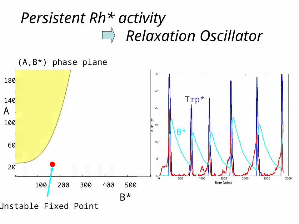
Persistent Rh* activity Relaxation Oscillator

20

60

100

140

180

100 200 300 400 500

Trp*

B*

A

Unstable Fixed Point

(A,B*) phase plane

A

B*

QB trains: theory versus experiment

Qualitative but not quantitative agreement so far…

Model:Arrestin mutant (deficient in Rh* inactivation):

Predicted [Caex] dependence

Observed external [Ca2+] dependence

[Caext] mM

Coe

ff o

f va

riatio

n

Peak current

Henderson and Hardie, J.Physiol. (2000) 524.1, 179

What does one learn from the model?

e.g. Mechanisms/parameters controlling: Threshold for QB generation. QB amplitude fluctuations. Latency. Yield (or response failure rate) Latency distribution.

Functional dependences:e.g. dependence of everything on [Ca++ ]ext

Modeling methodology questions

• Need an intelligent method of searching the parameter space and of characterizing the parameter manifold ??? How does Evolution search the parameter space?

• Characterizing the “space of models”??

• “Convergence proof”?? Given a model that fits N measurements can we expect that it will fit N+1 (even with additional parameters)?

• How accurate should a prediction be for us to believe that the model is correct ?? Unique??

Summary and Conclusion

A phenomenological model can explain observations and make numerous falsifiable predictions (especially for the functional dependence on parameters).

Insight into HOW the system works from understandingthe most relevant parameters and processes.

?????Can one get any insight into WHY the system is constructed the way it is (e.g. vertebrate versus insect) ?????

Acknowledgements

Alain Pumir, (Inst Non-Lineare Nice, France)

Rama Ranganathan (U. Texas,SW Medical School)

Anirvan Sengupta, (Rutgers)

Peter Detwiler (U. Washington)

Sharad Ramanathan (Harvard)