cop 3503 fall 2012 shayan javed lecture 15
DESCRIPTION
COP 3503 FALL 2012 Shayan Javed Lecture 15. Programming Fundamentals using Java. Algorithms Searching. So far. Focused on Object-Oriented concepts in Java Going to look at some basic computer science concepts: algorithms and more data structures. Algorithm. - PowerPoint PPT PresentationTRANSCRIPT

1 / 81
COP 3503 FALL 2012SHAYAN JAVED
LECTURE 15
Programming Fundamentals using Java
1

2 / 81
Algorithms
Searching

3 / 81
So far...
Focused on Object-Oriented concepts in Java
Going to look at some basic computer science concepts: algorithms and more data structures.

4 / 81
Algorithm
An algorithm is an effective procedure for solving a problem expressed as a finite sequence of instructions.
“effective procedure” = program

5 / 81
Pseudocode
A compact and informal description of algorithms using the structural conventions of a programming language and meant for human reading.

6 / 81
Pseudocode
A compact and informal description of algorithms using the structural conventions of a programming language and meant for human reading.
A text-based design tool that helps programmers to develop algorithms.

7 / 81
Pseudocode
A compact and informal description of algorithms using the structural conventions of a programming language and meant for human reading.
A text-based design tool that helps programmers to develop algorithms. Basically, write out the algorithm in steps which
humans can understand and can be converted to a programming language

8 / 81
Searching
Ability to search data is extremely crucial.

9 / 81
Searching
Ability to search data is extremely crucial.
Searching the whole internet is always a problem. (Google/Bing/...Altavista).

10 / 81
Searching
Ability to search data is extremely crucial.
Searching the whole internet is always a problem. (Google/Bing/...Altavista). Too complex of course.

11 / 81
Searching
The problem: Search an array A.

12 / 81
Searching
The problem: Search an array A.
N – Number of elements in the array

13 / 81
Searching
The problem: Search an array A.
N – Number of elements in the array k – the value to be searched

14 / 81
Searching
The problem: Search an array A.
N – Number of elements in the array k – the value to be searched
Does k appear in A?

15 / 81
Searching
The problem: Search an array A.
N – Number of elements in the array k – the value to be searched
Does k appear in A? Output: Return index of k in A

16 / 81
Searching
The problem: Search an array A.
N – Number of elements in the array k – the value to be searched
Does k appear in A? Output: Return index of k in A Return -1 if k does not appear in A

17 / 81
Linear Search
How would you search this array of integers?
(For ex., we want to search for 87)
i 0 1 2 3 4 5
A 55 19 100 45 87 33

18 / 81
Linear Search
How would you search this array of integers?
(For ex., we want to search for 87) Pseudocode:
for i = 0 till N: if A[i] == k return ireturn -1
i 0 1 2 3 4 5
A 55 19 100 45 87 33

19 / 81
Linear Search
int linearSearch (int[] A, int key, int start, int end)
{
for (int i = start; i < end; i++) {
if (key == A[i]) {
return i; // found - return index
}
}
// key not found
return -1;
}

20 / 81
Linear Search
int linearSearch (int[] A, int key, int start, int end)
{
for (int i = start; i < end; i++) {
if (key == A[i]) {
return i; // found - return index
}
}
// key not found
return -1;
}
int index = linearSearch(A, 87, 0, A.length);

21 / 81
Linear Search
Advantages: Straightforward algorithm.

22 / 81
Linear Search
Advantages: Straightforward algorithm. Array can be in any order.

23 / 81
Linear Search
Advantages: Straightforward algorithm. Array can be in any order.
Disadvantages: Slow and inefficient (if array is very large)

24 / 81
Linear Search
Advantages: Straightforward algorithm. Array can be in any order.
Disadvantages: Slow and inefficient (if array is very large)
N/2 elements on average (4 comparisons for 45)
25 / 81
Linear Search
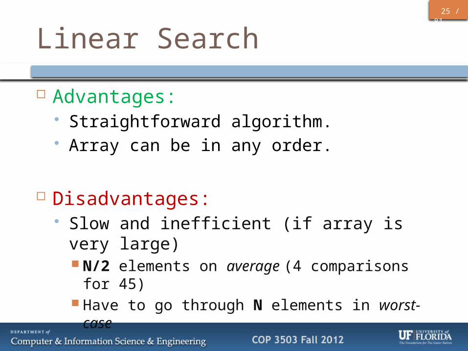
Advantages: Straightforward algorithm. Array can be in any order.
Disadvantages: Slow and inefficient (if array is very large)
N/2 elements on average (4 comparisons for 45) Have to go through N elements in worst-case

26 / 81
Algorithm Efficiency
How do we judge if an algorithm is good enough?

27 / 81
Algorithm Efficiency
How do we judge if an algorithm is good enough?
Need a way to describe algorithm efficiency.

28 / 81
Algorithm Efficiency
How do we judge if an algorithm is good enough?
Need a way to describe algorithm efficiency.
We use the Big O notation

29 / 81
Big O notation
Estimates the execution time in relation to the input size.

30 / 81
Big O notation
Estimates the execution time in relation to the input size.
Upper bound on the growth rate of the function. (In terms of the worst-case)

31 / 81
Big O notation
Estimates the execution time in relation to the input size.
Upper bound on the growth rate of the function. (In terms of the worst-case)
Written as O(x), where x = in terms of the input size.

32 / 81
Big O notation
If execution time is not related to input size, algorithm takes constant time: O(1).

33 / 81
Big O notation
If execution time is not related to input size, algorithm takes constant time: O(1). Ex.: Looking up value in an array – A[3]

34 / 81
Big O notation
If execution time is not related to input size, algorithm takes constant time: O(1). Ex.: Looking up value in an array – A[3]
Big O for Linear Search?

35 / 81
Big O notation
If execution time is not related to input size, algorithm takes constant time: O(1). Ex.: Looking up value in an array – A[3]
Big O for Linear Search? O(N) = have to search through at least N values of the
Array A
36 / 81
Big O notation
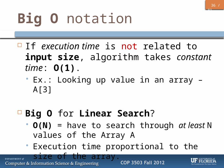
If execution time is not related to input size, algorithm takes constant time: O(1). Ex.: Looking up value in an array – A[3]
Big O for Linear Search? O(N) = have to search through at least N values of the
Array A Execution time proportional to the size of the array.

37 / 81
Big O notation
Another example problem: Find max value in an array A of size N.

38 / 81
Big O notation
Another example problem: Find max value in an array A of size N.
int max = A[0];
for i = 1 till i = N
if (A[i] > max)
max = A[i]
39 / 81
Big O notation
Another example problem: Find max value in an array A of size N.
int max = A[0];
for i = 1 till i = N
if (A[i] > max)
max = A[i]
How many comparisons?
N – 1 comparisons
Efficiency: O(n-1)
O(n) [Ignore non-dominating part]

40 / 81
Big O notation
Another example problem: Find max value in an array A of size N.
int max = A[0];
for i = 1 till i = N
if (A[i] > max)
max = A[i]
How many comparisons?
N – 1 comparisons
Efficiency: O(n-1)
O(n) [Ignore non-dominating part]

41 / 81
Big O notation
Another example problem: Find max value in an array A of size N.
int max = A[0];
for i = 1 till i = N
if (A[i] > max)
max = A[i]
How many comparisons?
N – 1 comparisons
Efficiency: O(N-1)
O(n) [Ignore non-dominating part]

42 / 81
Big O notation
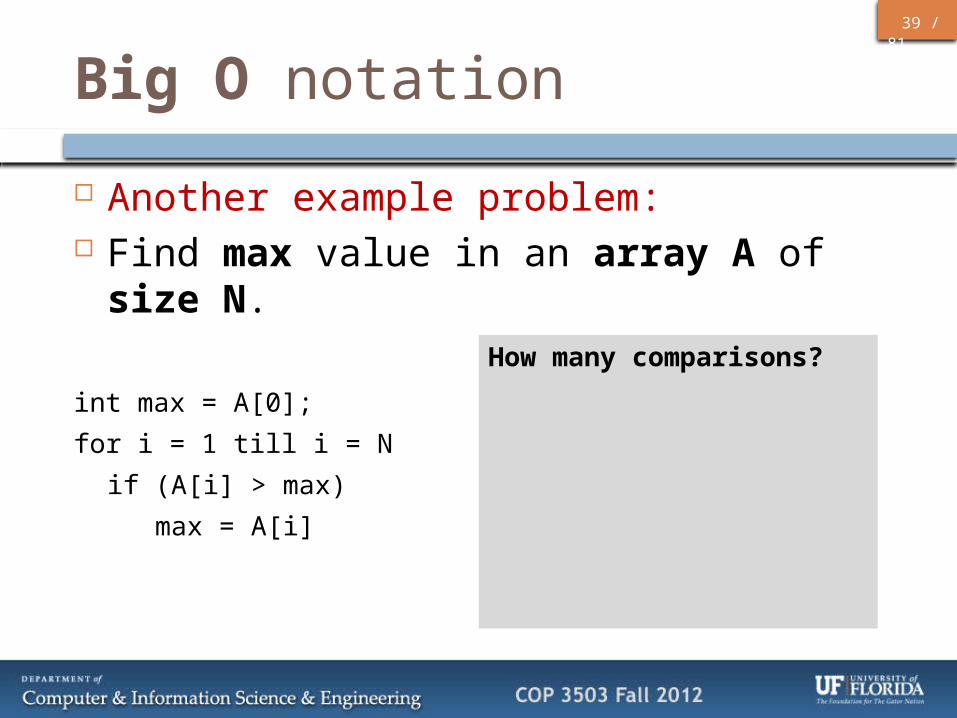
Another example problem: Find max value in an array A of size N.
int max = A[0];
for i = 1 till i = N
if (A[i] > max)
max = A[i]
How many comparisons?
N – 1 comparisons
Efficiency: O(N-1)
O(N) [Ignore non-dominating part]

43 / 81
Back to Search...
Linear Search is the simplest way to search an array.

44 / 81
Back to Search...
Linear Search is the simplest way to search an array.
Other data structures will make it easier to search for data.
45 / 81
Back to Search...
Linear Search is the simplest way to search an array.
Other data structures will make it easier to search for data.
But what if data is sorted?

46 / 81
Search
Array A of size 6: (search for k = 87)
A sorted:
i 0 1 2 3 4 5
A 19 33 45 55 87 100
i 0 1 2 3 4 5
A 55 19 100 45 87 33

47 / 81
Search
A sorted: k = 87
How can you search this more efficiently?
i 0 1 2 3 4 5
A 19 33 45 55 87 100

48 / 81
Search
A sorted: k = 87
How can you search this more efficiently?
Let’s start by looking at the middle index: I = N/2 = 3
i 0 1 2 3 4 5
A 19 33 45 55 87 100

49 / 81
Search
A sorted: k = 87
How can you search this more efficiently?
Let’s start by looking at the middle index: I = N/2 = 3
i 0 1 2 3 4 5
A 19 55 33 45 87 100
i 0 1 2 3 4 5
A 19 33 45 55 87 100

50 / 81
Search
A sorted: k = 87, I = 3
is 87 == A[I] ? No.
i 0 1 2 3 4 5
A 19 55 33 45 87 100
i 0 1 2 3 4 5
A 19 33 45 55 87 100

51 / 81
Search
A sorted: k = 87, I = 3
is 87 == A[I] ? No.
is 87 < A[I] ? No. (So 87 is NOT in index 0 through 3).
i 0 1 2 3 4 5
A 19 55 33 45 87 100
i 0 1 2 3 4 5
A 19 33 45 55 87 100

52 / 81
Search
A sorted: k = 87, I = 3
is 87 == A[I] ? No.
is 87 < A[I] ? No. (So 87 is NOT in index 0 through 3).
is 87 > A[I] ? Yes. (Now search from index 4 through 5).
i 0 1 2 3 4 5
A 19 33 45 55 87 100

53 / 81
Search
A sorted: k = 87
New index: I = (3 + N)/2 = 4.
i 0 1 2 3 4 5
A 19 33 45 55 87 100

54 / 81
Search
A sorted: k = 87, I = 4
New index: I = (3 + N)/2 = 4. Repeat the process.
i 0 1 2 3 4 5
A 19 55 33 45 87 100
i 0 1 2 3 4 5
A 19 33 45 55 87 100

55 / 81
Search
A sorted: k = 87, I = 4
New index: I = (3 + N)/2 = 4. Repeat the process. is 87 == A[I] ?
Yes! We found the index. Return I
i 0 1 2 3 4 5
A 19 55 33 45 87 100
i 0 1 2 3 4 5
A 19 33 45 55 87 100

56 / 81
Search
A sorted: k = 87, I = 4
New index: I = (3 + N)/2 = 4. Repeat the process. is 87 == A[I] ?
Yes! We found the index. Return I
This algorithm is called Binary Search
i 0 1 2 3 4 5
A 19 33 45 55 87 100

57 / 81
Search
Comparisons for Binary Search: 2
i 0 1 2 3 4 5
A 19 55 33 45 87 100
i 0 1 2 3 4 5
A 19 33 45 55 87 100

58 / 81
Search
Comparisons for Binary Search: 2
Comparisons for Linear Search: 5
i 0 1 2 3 4 5
A 19 55 33 45 87 100
i 0 1 2 3 4 5
A 19 33 45 55 87 100

59 / 81
Binary Search
For sorted data

60 / 81
Binary Search
For sorted data
Idea: Start at the middle index, then halve the search space for each pass.
61 / 81
Binary Search
Algorithm:

62 / 81
Binary Search
Algorithm:1. Get the middle element M between
index O and N

63 / 81
Binary Search
Algorithm:1. Get the middle element M between
index O and N2. if M = k, stop.

64 / 81
Binary Search
Algorithm:1. Get the middle element M between
index O and N2. if M = k, stop.3. Otherwise two cases:

65 / 81
Binary Search
Algorithm:1. Get the middle element M between
index O and N2. if M = k, stop.3. Otherwise two cases:
1. k < M, repeat from step 1 between O and M

66 / 81
Binary Search
Algorithm:1. Get the middle element M between
index O and N2. if M = k, stop.3. Otherwise two cases:
1. k < M, repeat from step 1 between O and M2. k > M, repeat from step 1 between M and N

67 / 81
Binary Search
int binarySearch(int[] array, int key, int left, int right){
while (left < right) {
int middle = (left + right)/2; // Compute mid point
if (key < array[mid]) {
right = mid; // repeat search in bottom half
} else if (key > array[mid]) {
left = mid + 1; // Repeat search in top half
} else {
return mid; // found!
}
}
return -1; // Not found
}

68 / 81
Binary Search
int binarySearch(int[] array, int key, int left, int right){
while (left <= right) {
int middle = (left + right)/2; // Compute mid point
if (key < array[mid]) {
right = mid; // repeat search in bottom half
} else if (key > array[mid]) {
left = mid + 1; // Repeat search in top half
} else {
return mid; // found!
}
}
return -1; // Not found
}

69 / 81
Binary Search
int binarySearch(int[] array, int key, int left, int right){
while (left <= right) {
int middle = (left + right)/2; // Compute mid point
if (key < array[mid]) {
right = mid; // repeat search in bottom half
} else if (key > array[mid]) {
left = mid + 1; // Repeat search in top half
} else {
return mid; // found!
}
}
return -1; // Not found
}

70 / 81
Binary Search
int binarySearch(int[] array, int key, int left, int right){
while (left <= right) {
int middle = (left + right)/2; // Compute mid point
if (key < array[mid]) {
right = mid-1; // repeat search in bottom half
} else if (key > array[mid]) {
left = mid + 1; // Repeat search in top half
} else {
return mid; // found!
}
}
return -1; // Not found
}

71 / 81
Binary Search
int binarySearch(int[] array, int key, int left, int right){
while (left <= right) {
int middle = (left + right)/2; // Compute mid point
if (key < array[mid]) {
right = mid-1; // repeat search in bottom half
} else if (key > array[mid]) {
left = mid + 1; // Repeat search in top half
} else {
return mid; // found!
}
}
return -1; // Not found
}

72 / 81
Binary Search
int binarySearch(int[] array, int key, int left, int right){
while (left <= right) {
int middle = (left + right)/2; // Compute mid point
if (key < array[mid]) {
right = mid-1; // repeat search in bottom half
} else if (key > array[mid]) {
left = mid + 1; // Repeat search in top half
} else {
return mid; // found!
}
}
return -1; // Not found
}

73 / 81
Binary Search
Exercise: Implement binary search recursively.

74 / 81
Binary Search
Advantages: Fast and efficient
Disadvantages: Has to be sorted first. (Going to look at sorting later)

75 / 81
Binary Search Efficiency
O(log2N)

76 / 81
Binary Search Efficiency
O(log2N)
Much faster than O(N).

77 / 81
Binary Search Efficiency
O(log2N)
Much faster than O(N). For N = 6, at most 2 comparisons. ⌊log2(N) + 1⌋

78 / 81
Binary Search Efficiency
O(log2N)
Much faster than O(N). For N = 6, at most 2 comparisons. ⌊log2(N) + 1⌋
N = 1 million.

79 / 81
Binary Search Efficiency
O(log2N)
Much faster than O(N). For N = 6, at most 2 comparisons. ⌊log2(N) + 1⌋
N = 1 million. Linear search = 1 million iterations

80 / 81
Binary Search Efficiency
O(log2N)
Much faster than O(N). For N = 6, at most 2 comparisons. ⌊log2(N) + 1⌋
N = 1 million. Linear search = 1 million iterations Binary search = 20 iterations

81 / 81
Summary
Search is an essential problem.
Linear search for an unsorted array.
Binary search for a sorted array.
Next Lecture: Sorting arrays