coordinate transformations: jacobians - university of · pdf file ·...
TRANSCRIPT
1
Coordinate transformations: Jacobians It is often advantageous to solve problems in other coordinates than Cartesian x, y, z system. We have already mentioned polar coordinates in 2D, and spherical and cylindrical coordinates in 3D. In general, we have transformation equations, which specify one coordinate system in terms of the other, such as:
),,(
),,(
),,(
321
321
321
uuuhz
uuugy
uuufx
where x, y, z are Cartesian coordinates, and u1, u2, u3 are some other coordinates (we are assuming 3D, but this would work in any dimension). The functions f, g and h establish a one-to-one correspondence between the coordinate systems: they have to be continuous, have continuous partial derivatives and single valued inverse (otherwise it would not be one-to-one). In vector notation, a point in space is:
),,(),,(),,(),,( 321321321321 uuuuuuhuuuguuufzyx rkjikjir
Just like x, y, z form a grid of straight lines in space, the u1, u2, u3 will define a grid of lines (not necessarily straight). For example, by keeping y and z constant and varying x, r will trace a line parallel to x axis. In the same way, keeping u2, u3 constant and varying u1 the r vector will describe a curve, which we call the u1 coordinate curve. Coordinate curves for u2 and u3 are defined the same way. From the above equation:
33
22
11
duu
duu
duu
d
rrr
r
As we already know,
1ur
is a vector, that is tangent to the coordinate curve u1 (same for u2 and u3 ).
Therefore, if e1, e2 and e3 are unit vectors in the tangent direction to u1, u2 and u3 respectively, we have:
33333
22222
11111
eerr
eerr
eerr
huu
huu
huu
where we have defined the scale factors 3
32
21
1 ,,u
hu
hu
h
rrr
and we can rewrite the previous equation as:
333222111 eeer duhduhduhd
which is the differential of the vector in the new coordinates, u1, u2, u3.

2
If e1, e2 and e3 are mutually orthogonal at any particular point, the coordinates are called orthogonal. Orthogonal coordinates make things simple. For example, the square of arc length (e.g. a piece of trajectory travelled by a particle) is given as:
22
22
22
22
21
21
2 duhduhduhddds rr What is important for calculating integrals in 3D space, is the volume element dV (in 2D it would be an area element). By virtue of orthogonal coordinates:
321321333222111 )()( dududuhhhduhduhduhdxdydzdV eee
which can be written as:
321
321321
321 ,,
,,dududu
uuu
zyxdududu
uuudV
rrr
where:
321
321
321
321
det,,
,,
u
z
u
z
u
zu
y
u
y
u
yu
x
u
x
u
x
uuu
zyx
is the Jacobian determinant , or shortly Jacobian.
Gradient, Divergence, Curl and Laplacian in curvilinear orthogonal coordinates For a scalar function and vector function A = A1e1+ A2e2+ A3e3 in orthogonal curvilinear coordinates u1, u2, u3 the following general formulas can be derived:
3213
2312
1321321
333
222
111
1div
111grad
Ahhu
Ahhu
Ahhuhhh
uhuhuh
AA
eee
3
332211
321
332211
321
det1
curl
AhAhAhuuu
hhh
hhh
eee
AA
33
21
322
31
211
32
1321
2 1
uh
hh
uuh
hh
uuh
hh
uhhh
Important special cases of curvilinear coordinates
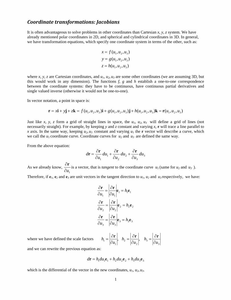
2D: Plane polar coordinates:
x= r cos() y= r sin()
0< r <, 0< Scale factors: h1 =1, h2 =r
Jacobian: r
uu
yx
21,
,
Volume element: dV = rdrd
3D: Spherical polar coordinates:
x= r sin( cos() y= r sin() sin() z= r cos()
0< r <, 0< < <, Scale factors: h1 =1, h2 =r, h3 = rsin
Jacobian: sin
,,
,, 2
321
ruuu
zyx
Volume element: dV = r2 sin drd d
4
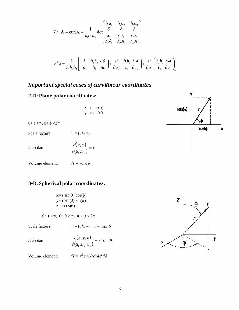
3D: Cylindrical coordinates:
x= cos()
y= sin() z= z
0< <, 0< < z <, Scale factors: h1 =1, h2 =, h3 = 1
Jacobian:
321 ,,
,,
uuu
zyx
Volume element: dV = d ddz
5
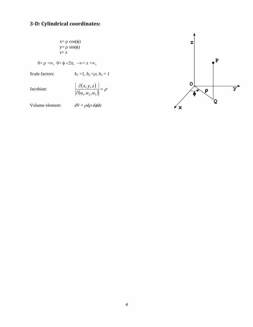
Double integrals Double integral is an integral over an area in 2D space. There can also be a double integral in 3D space, but that is called a surface integral. The double integral is defined in analogy to the 1-D Riemann sum:
n
kkkk
An
AyxFdxdyyxF1
),(lim),(
where Ak are some smaller pieces into which the area over which we integrate is subdivided. If the area of integration is a simple shape, i.e. if any line parallel to x an y axes meet the boundary in at most two points, then we can write the upper and lower curves, which bound the area, as functions of x: y1 = f(x) and y 2=g(x) (below, left)
Then we can integrate first with respect to y from the lower boundary (y1) to the upper (y 2), but remember these are now functions of x. This integration will yield a function of x, because the limits are functions of x. In the second step we integrate over x between its limits (a, b) , which are constants. Note that (definite) integral has to produce a number a not a function:
A
b
a
xgy
xfy
dxdyyxFdxdyyxF)(
)(
2
1
),(),(
We can, of course, do it the other way by defining the left and right boundaries as functions
x1 = u(y) and
x2 = v(y) (figure above, right). Then we integrate over x first (between the function limits) and then y between its limits (b, c):
6
A
d
c
xvx
yux
dydxyxFdxdyyxF)(
)(
2
1
),(),(
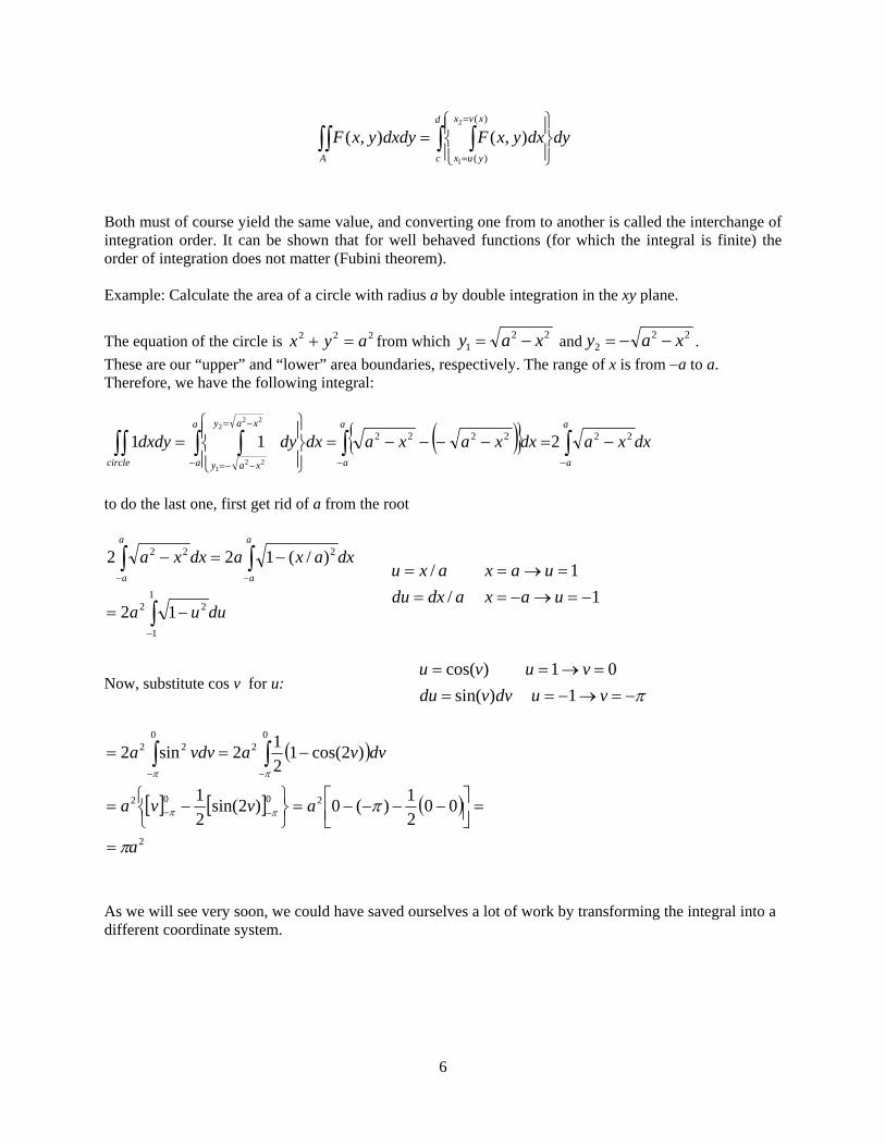
Both must of course yield the same value, and converting one from to another is called the interchange of integration order. It can be shown that for well behaved functions (for which the integral is finite) the order of integration does not matter (Fubini theorem). Example: Calculate the area of a circle with radius a by double integration in the xy plane.
The equation of the circle is 222 ayx from which 221 xay
and 22
2 xay .
These are our “upper” and “lower” area boundaries, respectively. The range of x is from a to a. Therefore, we have the following integral:
a
a
a
acircle
a
a
xay
xay
dxxadxxaxadxdydxdy 222222 211
222
221
to do the last one, first get rid of a from the root
1
1
22
222
12
)/(122
duua
dxaxadxxaa
a
a
a
1/
1/
uaxadxdu
uaxaxu
Now, substitute cos v for u:
vudvvdu
vuvu
1)sin(
01)cos(
2
2002
02
022
002
1)(0)2sin(
2
1
)2cos(12
12sin2
a
avva
dvvavdva
As we will see very soon, we could have saved ourselves a lot of work by transforming the integral into a different coordinate system.
7
Triple integrals Triple integrals are integrals over a three dimensional region (volume) in three dimensions. Everything we have just done for double integrals can be generalized to three dimensions. I.e. the integral is defined as the limit of a sum over some finite subdividing elements when the number of elements approaches infinity (and their individual volumes go to zero):
n
kkkkk
nV
VzyxFdxdydzzyxF1
),,(lim),,(
The integral can be again iterated, i.e. evaluated one integration variable at a time. Now, however, the first set of limits would be functions of the two remaining variables, the second set of limits a function of the remaining single one and the last set of limits constants. For example:
b
ax
xg
xfy
yxv
yxuzV
dxdydzzyxFdxdydzzyxF)(
)(
),(
),(
),,(),,(
Again, the order of integration is interchangeable for any well behaved functions.
Example: Integral of some function F(x, y, z) over a curve given by equation 2222 azyx (sphere)
would look like:
a
ax
xay
xay
yxaz
yxazsphere
dxdydzzyxFdxdydzzyxF
222
221
2222
2221
),,(),,(
Again, this would be a lot easier in different coordinates. However, it illustrates how to set up the limits of integration: first in z (sphere) then in y (circle) and then x. Note that this is not the only way, we could have done x first, then y, then z etc. Often the region is given by several rules, e.g. intersections of shapes, planes etc. It helps to sketch it first to figure out the integration limits.
Transformations of multiple integrals As we have already discussed, in many cases it makes the evaluation of multiple much easier to use some other coordinates than Cartesian. In 2D for some general curvilinear coordinates u1, u2, whose transformation equations are:
),(
),(
21
21
uugy
uufx
we have:
A A
duduuu
yxuuGdxdyyxF 21
2121 ),(
),(),(),( where )),(),,((),( 212121 uuguufFuuG
and),(
),(
21 uu
yx
is the Jacobian, whom we have already met.
8
In 3D it is again the same story: if u1, u2 and u3, are our curvilinear coordinates, with transformations:
),,(
),,(
),,(
321
321
321
uuuhz
uuugy
uuufx
then
V
VV
dududuuuu
zyxuuuhuuuguuufF
dududuuuu
zyxuuuGdxdydzzyxF
321321
321321321
321321
321
),,(
),,()),,(),,,(),,,((
),,(
),,(),,(),,(
Example: Again, calculate the area of a circle with radius a. Now since we are allowed, we will transform the integral into plane polar coordinates:
22
0
2
0 0 2
1221 aardrrdrddxdy
aa
circle
Definitely a lot easier thane above. Similarly, for the sphere in 3D we would go to spherical coordinates:
3
3
0
30
0
22
0 0 0 0
2
3
4
03
1)1()1(2
3
1cos2
sin2sin),,(
a
ar
drdddrdrdxdydzzyxF
a
aa
sphere
9
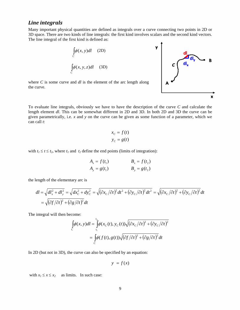
Line integrals Many important physical quantities are defined as integrals over a curve connecting two points in 2D or 3D space. There are two kinds of line integrals: the first kind involves scalars and the second kind vectors. The line integral of the first kind is defined as:
C
dlyx ),( (2D)
C
dlzyx ),,( (3D)
where C is some curve and dl is the element of the arc length along the curve. To evaluate line integrals, obviously we have to have the description of the curve C and calculate the length element dl. This can be somewhat different in 2D and 3D. In both 2D and 3D the curve can be given parametrically, i.e. x and y on the curve can be given as some function of a parameter, which we can call t:
)(
)(
tgy
tfx
C
C
with t1 t t2, where t1 and t2 define the end points (limits of integration):
)(
)(
1
1
tgA
tfA
y
x
)(
)(
2
2
tgB
tfB
y
x
the length of the elementary arc is
dttgtf
dttytxdttydttxdydxdldldl CCCCCCyx
22
2222222222
The integral will then become:
dttgtftgtf
tytxtytxdlyx
C
t
t
CCCC
C
22
22
))(),((
))(),((),(2
1
In 2D (but not in 3D), the curve can also be specified by an equation:
)(xfy
with x1 x x2 as limits. In such case:
10
dxdxdfxdydxdldldl yx22222 1)(
and
dxdxdfxyxdlyxx
xC
2
1
21))(,(),(
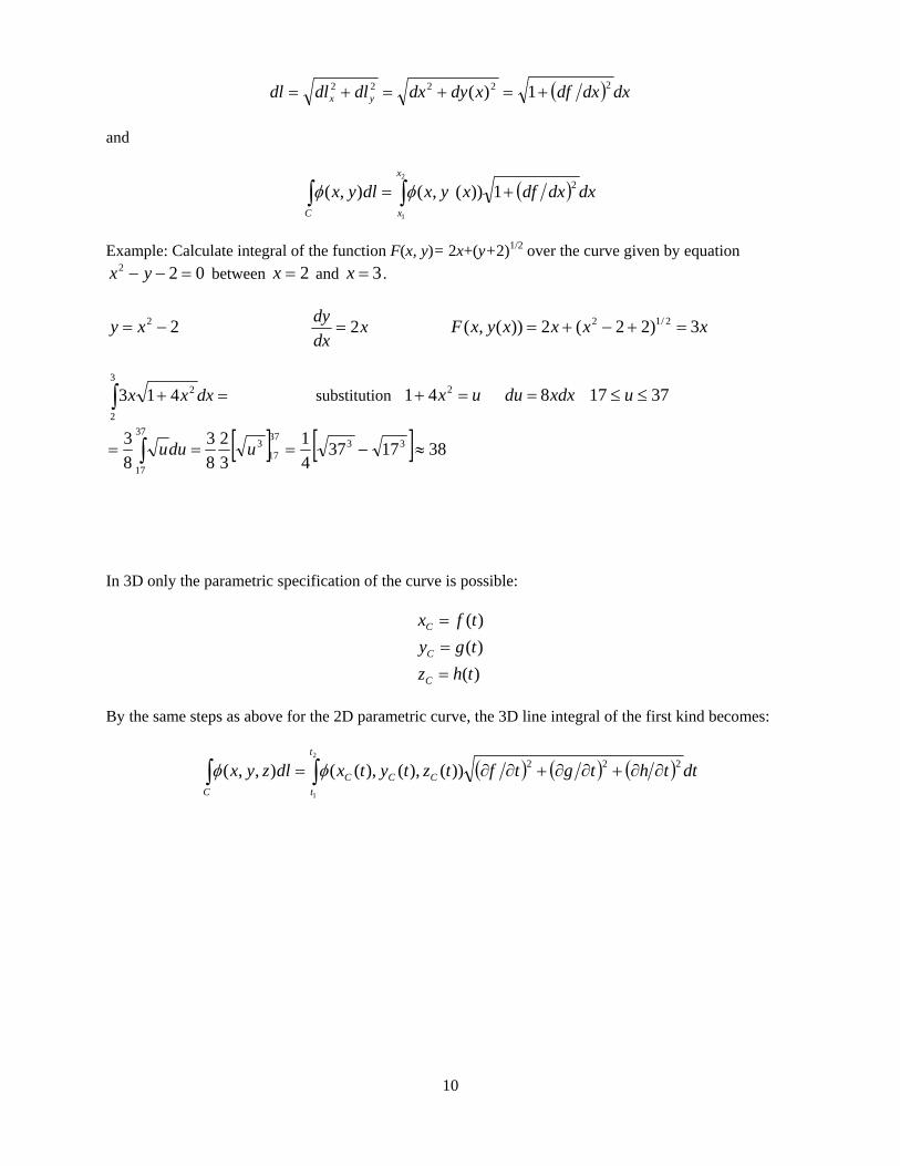
Example: Calculate integral of the function F(x, y)= 2x+(y+2)1/2 over the curve given by equation
022 yx between 2x and 3x .
22 xy xdx
dy2 xxxxyxF 3)22(2))(,( 2/12
dxxx3
2
2413 substitution 3717841 2 uxdxduux
3817374
1
3
2
8
3
8
3 3337
173
37
17
uduu
In 3D only the parametric specification of the curve is possible:
)(
)(
)(
thz
tgy
tfx
C
C
C
By the same steps as above for the 2D parametric curve, the 3D line integral of the first kind becomes:
2
1
222))(),(),((),,(t
t
CCC
C
dtthtgtftztytxdlzyx

11
The second kind of line integrals are those for vector fields. These actually have many more applications in physics and physical chemistry. For example, mechanical work done by moving a particle around some curve C in the field of force F(r) is given by:
C
dW rrF )(
The dot, as always, denotes scalar product: work is a scalar while force (F) and radius (position) vector (r) are vectors. By expanding the dot product into components, the integral simplifies:
C
zyx
C
dzzyxFdyzyxFdxzyxFdW ),,(),,(),,()( rrF
which looks like three simple integrals. However, we still need some sort of prescription for the curve. To change things up, we will do the 3D first. Since in 3D we only have parametric form:
)(
)(
)(
thz
tgy
tfx
C
C
C
by using chain rule (or substitution rule):
2
1
))(),(),(())(),(),(())(),(),((
),,(),,(),,()(
t
t
zyx
C
Cz
Cy
Cx
C
dtdt
dhthtgtfF
dt
dgthtgtfF
dt
dfthtgtfF
dtdt
dzzyxFdt
dt
dyzyxFdt
dt
dxzyxFdW rrF
this looks like an awfully complicated formula, but it actually is not that bad: we have three integrals with respect to t and no nasty square root as in the case of the first kind integrals above. In 2D the integral with parametric expression for the curve is very much the same, except there is no z :
2
1
))(),(())(),((),(),()(t
t
yx
C
yx
C
dtdt
dgtgtfF
dt
dftgtfFdyyxFdxyxFdW rrF
and if the curve is specified by the equation (remember, this is possible in 2D only):
)(xfy
we have:
2
1
))(,())(,()(x
x
yx
C
dxdx
dfxfxFdxxfxFdW rrF
12
Important properties of line integrals:
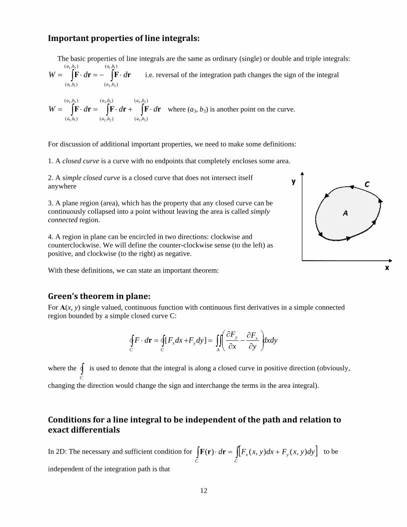
The basic properties of line integrals are the same as ordinary (single) or double and triple integrals:
),(
),(
),(
),(
11
22
22
11
ba
ba
ba
ba
ddW rFrF i.e. reversal of the integration path changes the sign of the integral
),(
),(
),(
),(
),(
),(
22
33
33
22
22
11
ba
ba
ba
ba
ba
ba
dddW rFrFrF where (a3, b3) is another point on the curve.
For discussion of additional important properties, we need to make some definitions: 1. A closed curve is a curve with no endpoints that completely encloses some area. 2. A simple closed curve is a closed curve that does not intersect itself anywhere 3. A plane region (area), which has the property that any closed curve can be continuously collapsed into a point without leaving the area is called simply connected region. 4. A region in plane can be encircled in two directions: clockwise and counterclockwise. We will define the counter-clockwise sense (to the left) as positive, and clockwise (to the right) as negative. With these definitions, we can state an important theorem:
Green’s theorem in plane: For A(x, y) single valued, continuous function with continuous first derivatives in a simple connected region bounded by a simple closed curve C:
dxdyy
F
x
FdyFdxFdF
A
xyy
C
x
C
][r
where the C
is used to denote that the integral is along a closed curve in positive direction (obviously,
changing the direction would change the sign and interchange the terms in the area integral).
Conditions for a line integral to be independent of the path and relation to exact differentials
In 2D: The necessary and sufficient condition for C
yx
C
dyyxFdxyxFd ),(),()( rrF to be
independent of the integration path is that

13
x
F
y
F yx
This condition is exactly the same as that dyFdxF yx is an exact differential, i.e. that there exists a
function ),( yx such that:
dyyxFdxyxFyxd yx ),(),(),(
In such case, if the points on the curve are ),( 11 yx and ),( 22 yx , the value of the line integral is:
),(),(),(),( 11
),(
),(
22
),(
),(
22
11
22
11
yxyxddyyxFdxyxFyx
yx
yx
yx
yx
Therefore the value depends only on the function at the end points (limits) of the integral and not on the particular path or curve that connects them. If the integral is done along the closed path, i.e.
),( 11 yx = ),( 22 yx then:
0),(),(),(),( 1111 yxyxdyyxFdxyxF yx
or, the integral along any closed path is zero. Note another important relationship between ),( yx FFF and :
yxyxFF
yF
xF
dyyxFdxyxFyxd
yx
y
x
yx
,,),(
),(),(),(
F
The vector field F is therefore a gradient of some scalar field . In this particular example, force is a gradient of some scalar function. If we define potential energy V as we will get back the relationship that we already know, namely that force is the negative gradient of the potential energy:
VF
Another incarnation of this relationship is electric field E which is nothing but gradient of the electric potential :
E
Generalization to 3D is again straightforward: the necessary condition for a line integral

14
C
zyx
C
dzzyxFdyzyxFdxzyxFd ),,(),,(),,()( rrF
to be independent of path is that the cross derivatives are all equal:
x
F
y
F yx
z
F
y
F yz
x
F
z
F zx
which is again equivalent to saying that dzFdyFdxF zyx is exact differential and F is gradient of
some scalar function: V F
In 3D, however, this condition can also be restated, by noticing that the cross derivatives above also mean that:
0FF
0,0,0,,curly
F
x
F
x
F
z
F
z
F
y
F xyzxyz
which commonly used as a condition for a conservative field, i.e. field which is given as a gradient of a scalar function (potential) and whose line integral between two points is independent of path (and along closed path always zero). If you recall one of the identities of the vector analysis: 0)( U or that curl grad(U) is always zero and combining that last two equations:
0
F
F
In other words, if F can be written as a gradient of some function, its curl will always be zero. Furthermore, integrals will be independent of path. All these statements are equivalent (one follows from the other) and all characterize the conservative (or potential) field.
Example: For jiA xyyx 22 evaluate the integral )2,1(
)1,0(
rΑ d a) along a straight line from
(0,1) to (1,2) b) along straight lines from (0,1) to (1,1) and then from (1,1) to (1,2) and c) along a parabola x = t, y=t2 +1. a) The straight line from (0,1) to (1,2) is given by equation y = x + 1, 0 x 1. Then dy/dx =1 and
3
522131
)1()1(
1
0
21
0
22
1
0
2222
dxxxdxxxdxxx
dxdxdyxxdxxxdyxydxyxdCC
rΑ
15
b) Straight line from (0,1) to (1,1) is given by y =1, dy = 0, 0 x 1. The line from (1,1) to (1,2) on the other hand by x =1, dx = 0 1 y 2. Therefore:
3
8
3
10
3
211
1)0(1)0(11
2
1
21
0
2
2
1
21
0
222
dyydxx
dyyyxdxxdyxydxyxdCC
rΑ
c) At (0,1), t =0 and at (1,2) t =1. Substituting for x, y, using the equation of the parabola, and using
tdt
dy
dt
dx2,1
the integral becomes:
1
0
245
1
0
222222
3
1012242
21)1(
dttttt
tdtttdtttdyxydxyxdCC
rΑ
Obviously, along each path the integral is different, which tells us that A is not a gradient of any scalar
function, or, equivalently, dyxydxyx 22 is not an exact differential. Example: Verify Green’s theorem in the plane for
CC
dyyxdxxxyd )()2( 22rΑ
where C is the closed curve around the region bounded by
2xy and xy 2 The curves intersect at (1,1), positive direction of traversing the closed curve is counterclockwise (see figure).
Along 2xy the integral equals:

16
6
7)22(
22
/)()(2
5231
0
1
0
423
1
0
2222
dxxxx
xdxxxdxxx
dxdxdyxxdxxxx
x
x
x
Along the other line xy 2 (now we are going from (1,1) back to (0,0)):
0
1
2540
1
243
0
1
22222
15
17224222
/)(2
yy
y
dyyyydyydyyyy
dyyydydydxyyy
The line integral is 30
1
15
17
6
7
From Green’s theorem in the plane:
dxdyx
dxdyy
xxy
x
yxdxdy
y
A
x
Ad
A
AA
xy
C
21
)2()( 22
rΑ
From the figure above we can iterate the integral, e.g. integrate first over y from 2x to x and then over x from 0 to 1:
30
1222)21(21
1
0
322/32/11
0
1
02
2
dxxxxxxyydydxxdxdyxxx
x
xy x
xxy
A
17
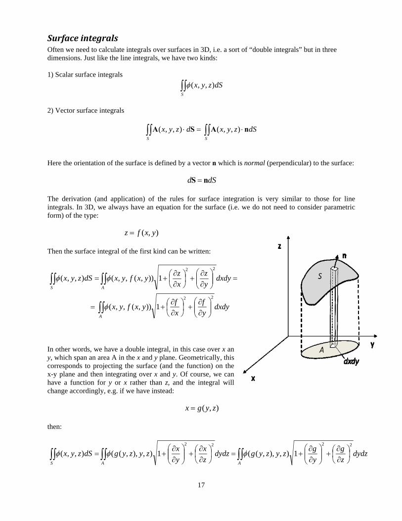
Surface integrals Often we need to calculate integrals over surfaces in 3D, i.e. a sort of “double integrals” but in three dimensions. Just like the line integrals, we have two kinds: 1) Scalar surface integrals
S
dSzyx ),,(
2) Vector surface integrals
SS
dSzyxdzyx nASA ),,(),,(
Here the orientation of the surface is defined by a vector n which is normal (perpendicular) to the surface:
dSd nS
The derivation (and application) of the rules for surface integration is very similar to those for line integrals. In 3D, we always have an equation for the surface (i.e. we do not need to consider parametric form) of the type:
),( yxfz
Then the surface integral of the first kind can be written:
A
AS
dxdyy
f
x
fyxfyx
dxdyy
z
x
zyxfyxdSzyx
22
22
1)),(,,(
1)),(,,(),,(
In other words, we have a double integral, in this case over x an y, which span an area A in the x and y plane. Geometrically, this corresponds to projecting the surface (and the function) on the x-y plane and then integrating over x and y. Of course, we can have a function for y or x rather than z, and the integral will change accordingly, e.g. if we have instead:
),( zygx
then:
AAS
dydzz
g
y
gzyzygdydz
z
x
y
xzyzygdSzyx
2222
1),),,((1),),,((),,(
18
The surface integral of the second kind again has a scalar product, which can be expanded:
S
zyx
SS
dxdyAdzdxAdydzAdSzyxdzyx nASA ),,(),,(
giving effectively three double integrals. Note, that in this case the projection is always on the plane perpendicular to the component of A (because we are multiplying by a normal vector), i.e. Ax is integrated in y-z plane etc. In practice, rather than three “perpendicular” integrals, the second kind surface integrals are evaluated by calculating the normal vector n to the surface, then doing the scalar product nA ),,( zyx turning it into the surface integral of the first kind, and then using one of the formulas given above to calculate that. To obtain the normal vectors, we can use the gradient operator. The gradient will always be perpendicular (normal) to a surface where a function has a constant value, i.e. for
.,, constzyzF
|||grad|
grad
F
F
F
F
n
This is very useful, because the general equations for the surface ),( yxfz can be easily turned into
this form, i.e. 0),( zyxf
Example: Evaluate S
dSzyx ),,( where S is the surface of the paraboloid )(2 22 yxz above the
xy plane, and zyx ),( .
dxdyyzxzyxdSzyxAS 2222 //1)2(),,( where A is the projection of the
paraboloid onto the x-y plane, i.e. z =0, which gives: 2)(20 2222 yxyx .The derivatives are:
xx
z2
and yy
z2
so that the integral becomes:
dxdyyxyxA 2222 441)2(
and we have a double integral. To evaluate this, we could iterate it (do the y first, then x) but it is much easier to do in polar coordinates (what gives it away is that we always have x2 + y2 which is r2 in polar
coordinates or that 222 yx is the equation of a circle), so we will transform it instead:
19
rdrrrrdrdrrdxdyyxyxrrA
2
0
222
0
2
0
222222 4122412441)2(
substitution ur 241 gives rdrdu 8 , 4/12 ur , 91 u
10
37
10
148
41243
10
1127
2
3
4
5
2
4
1
3
2
4
9
44
1
4
9
44/)1(2
8
2 9
12/59
12/3
9
1
2/39
1
2/19
0
uuduuduuduuuu
Example: Calculate the following integral:
S
dSE
where E = (0, 0, E0) and S is the surface of the hemisphere with the radius a, z 0.
Equation for the sphere is: 2222 azyx which we rewrite as 0),,( 2222 azyxzyxF . The normal vector is then:
222222
),,(
444
)2,2,2(
zyx
zyx
zyx
zyx
F
F
n
so that
222
0
2220
),,(),0,0(
zyx
zE
zyx
zyxE
nE
Since
222 yxaz
222222,
yxa
y
y
z
yxa
x
x
z
we have the following integral:
dxdyyxa
y
yxa
x
zyx
yxaEd
AS222
2
222
2
222
222
0 1
SE
where we now integrate over a circle (radius a) in the xy plane. We can considerably simplify this nasty integral:

20
20
2
0 0
00
222
222
222
22222
22222
222
0
222
aErdrdEdxdyE
dxdyyxa
a
a
yxadxdy
yxa
yxyxa
yxayx
yxaE
a
rayx
AA
Transformation of line and surface integrals Of course, the transformation rules, discussed for the double and triple integrals hold and often it is a great advantage to choose a different coordinate system. The last example could have been done easily in spherical coordinates (integral over a hemisphere). In fact, in the last step (double integral) we changed over to plane polar coordinates to the integral over the circle.
Green’s theorem (divergence theorem) If S is a closed surface bounding a region of volume V, the normal vector n is oriented to point to the outside of the surface. Then
SV
ddV SAAdiv
in other words:
SV
zyx ddVz
A
y
A
x
ASA
(of course, Ax, Ay, Az must have partial derivatives and they also have to be continuous). In words, the surface integral of a normal component of a vector A taken over a closed surface is equal to the integral of divergence of A over the volume enclosed by the surface. Physically, this means that the total flux of some quantity outwards through the surface equals to its divergence inside the enclosed volume.
Stokes’ theorem If S is an open two-sided surface bounded by a closed, non-intersecting curve C (simple closed curve). The sense of C is positive if an observer walking on the boundary with his head pointing in the direction of the positive normal n to the surface has the surface on its left (the right hand rule: fingers in the direction of circling, thumb points in the positive n direction).
21
Then:
SSC
ddd SASArA curl
In words: line integral of the vector A taken over a simple closed curve C is equal to the surface integral of the normal component of the curl of A taken over any surface S having C as its boundary.
Note that if 0 A the integral over the closed path is identically zero: 0C
drA which is the case
of the conservative field, discussed above.