COOPERATIVE GAMES AND BUSINESS STRATEGY

H. W. Stuart, Jr.

[This paper appeared as Chapter 6, pages 189-211, Game Theory and Business Applications, K. Chatterjee and W. F. Samuelson, eds, Kluwer, Boston/Dordrecht/London, 2001.] The main purpose of this chapter is to demonstrate how cooperative game theory can be applied to business strategy. Although the academic literature on cooperative game theory is extensive, very little has been written from a strategy perspective. The situation with textbooks is similar. With few exceptions (e.g., Oster, 1994), strategy textbooks generally do not mention cooperative game theory. In fact, the most visible applications of cooperative game theory to strategy have been in the popular press, MacDonald’s The Game of Business1 (1975) and Brandenburger and Nalebuff’s Co-opetition (1996), for example. The material in this chapter is taken from academic papers and teaching notes that use cooperative game theory for analyzing business strategy. Applying cooperative game theory to strategy often results in suggestive interpretations; this chapter will emphasize these interpretations since they are, arguably, a significant benefit of using cooperative game theory.

A cooperative game consists of a player set and a function specifying how much value any subset of players can create. This sparse formalism can be used to model situations in which there are no restrictions on the interactions between players. Players are free to pursue any favorable deals possible, and, in particular, no player is assumed to have price-setting power. For this reason, cooperative game theory can be considered a structural, rather than procedural, theory. It specifies the structure of the game: who the players are

2

and what value they might appropriate. But it does not specify the procedures for creating and dividing value.

The structural approach of cooperative game theory has certain advantages for the study of business strategy. Since many business interactions are free-form in nature, this might not seem so surprising. But there are other benefits that this chapter will demonstrate. The effects of competition can be clearly identified in the analysis of a cooperative game. Although price-setting power is not assumed in a cooperative game, it can emerge from the structure of the game.2 And even the process of formulating the game yields insights, as it often requires that basic business questions be answered. The non-procedural nature of cooperative game theory may also be viewed as one of its limitations. In situations in which the players’ interactions must follow well-defined rules, the free-form nature of a cooperative game probably will not be desirable. The question of uncertainty poses another limitation. To date, uncertainty has not been integrated into the application of cooperative game theory to business strategy, and attempts to do so have been informal at best. Section 1 of this chapter reviews the definition of a cooperative game. For business strategy, cooperative games will be analyzed by methods that model unrestricted bargaining. With unrestricted bargaining, players are assumed to be actively involved in the creation and division of value. Unrestricted bargaining can be modeled by either the core of the game or the added value principle. The core is a more traditional method of analysis, but in business strategy, the added value principle often suffices. This section provides both definitions. To examine actual cooperative games for business strategy, Section 1 uses the Supplier-Firm-Buyer game. This game is used to demonstrate how competition, reflected in players' added values, can either partially or completely determine the division of value. Further, the discussion of added value in these games introduces some of the basic business questions. Business strategy is as much about creating a favorable game for yourself as it is about doing well in some existing game. Section 2 introduces a game form, called a biform game, for analyzing situations in which players have the ability to affect what business game they play.3 Two examples are provided. First, a familiar monopoly example demonstrates both the approach

3

and the relationship between monopoly power and competition. The second example is a biform model of spatial competition, in which socially-efficient, spatial differentiation can be a stable outcome.

1. The Game of Business as a Cooperative Game

Cooperative Games

A transferable-utility (TU) cooperative game is composed of a finite set N and a mapping Nv 2: . The set N denotes the set of players, and the mapping v, the characteristic function, specifies, for each subset of the players, the value created by the subset. Thus, for any NS , v(S) is the maximum economic value that the players

in S can create among themselves.

An outcome of a cooperative game (N; v) is described by a vector N

x . This vector specifies both the total value created and how it is divided. The component xi

denotes the value captured by player i. And the total value created, namely x(N), is

then Ni ix .

Definition: For any NS , let Si ixSx )( . The core of a TU cooperative game

(N; v) is the set of outcomes satisfying x(N) = v(N) and )()(, SvSxNS .

Definition: The added value of a coalition NS is defined to be the coalition’s marginal contribution: )\()( SNvNv . (The term v(N \ S) denotes the value created by

the coalition consisting of all players except the players in S.) The added value of a given player, say i, is therefore }){\()( iNvNv . An outcome satisfies the added value

principle if no player captures more than its added value, that is, if: }){\()(, iNvNvxNi i , and if x(N) = v(N).

The added value principle generates a superset of the core; that is, core outcomes must satisfy the added value principle. To see this, consider a given player i. The two conditions x(N) = v(N) and }){\(}){\( iNviNx imply the added value condition

}){\()( iNvNvxi .

4

Both the core and the added value principle can be interpreted as modeling unrestricted bargaining. With unrestricted bargaining, all players are actively involved in seeking out favorable transactions, and no player is assumed to have any price-setting power. Further, any player or group of players is free to pursue a more favorable deal. For both the added value principle and the core, the mathematical statements generating these interpretations can be identified. With the added value principle, it is implied by the equation }){\()( iNvNvxi . If a player were to

receive more than its added value, namely }){\()( iNvNvxi , then it would have to

be the case that }){\(}){\( iNviNx . But if this were so, the group N\{i} would prefer

to actively pursue a deal on its own, thus obtaining v(N\{i}) of value. In other words, if a given player were to receive more than its added value, then the other players would do better by excluding that player from the game. With the core, a similar interpretation holds. But, whereas the unrestricted-bargaining interpretation of the added value principle considers only coalitions of the form N\{i}, the interpretation for the core considers any coalition. If any coalition, say S, anticipated capturing less value than it could create on its own, namely x(S) < v(S), then it would create and divide v(S) of value on its own. This interpretation is consistent with the core condition that )()(, SvSxNS .

With any group of players free to create value on its own, Aumann (1985, pg. 53) states that the core captures the notion of “unbridled competition.” The idea that a core analysis can model competition dates back to Edgeworth (1881). As Shubik (1959) discovered, Edgeworth’s reasoning about “contracting” and “re-contracting” is consistent with the core conditions. But this “competition” does not necessarily determine a unique outcome. For a given player, the core will usually specify a range of values rather than a single amount. The minimum of the range is interpreted as the amount of value guaranteed the player due to competition. The difference between the minimum and the maximum is then interpreted as a residual bargaining problem. With an added value analysis, the interpretation is the same. If the added value principle implies a minimum amount for a player, then this is the amount due to competition. If the added value principle allows the player to capture more than this minimum, then the difference is a residual bargaining problem.

5

Supplier-Firm-Buyer Games4

Shapley and Shubik (1972) use two-sided assignment games to gain insights into buyer-seller markets with small numbers of players. Since business strategy is often concerned with small buyer-seller interactions, this suggests that assignment games might provide a natural starting point for applying cooperative game theory to business strategy. But since strategy focuses on the firm, it is convenient to start with a three-sided assignment game. Three sides are useful since the firm is both a buyer and a seller -- a buyer with respect to its suppliers and a seller with respect to its customers. Definition: A three-sided assignment game consists of three disjoint sets, N1, N2,

N3, and a three-dimensional assignment matrix, A. The matrix has dimensions of

321 nnn , where || 11 Nn , etc. (Alternatively, the assignment matrix is a mapping

321: NNNA .) The disjoint sets are interpreted as sets of players. A matching

is a 3-tuple ijk consisting of a player i from set N1, a player j from set N2, and a

player k from set N3. Element ijka of the matrix A is interpreted as the value that can

be created by the matching ijk. Two matchings aaa kji and bbb kji are distinct if

bababa kkjjii ,, . An assignment of size r is a set of r distinct matchings.

The construction of the TU cooperative game for an m-sided assignment game is based on two principles. First, value creation is determined solely by distinct matchings, and second, the value created is taken to be as large as feasibly possible. Equations (1) – (3) below incorporate these principles. Define the player set, N, to be 321 NNN . The characteristic function v is defined

by 0)( v , and, for all T N,

,}3,2,1{ , if 0)( mNTTv m (1)

,,,}),,({ 321 NkNjNiakjiv ijk and (2)

)(max)( 111

,rrr kjikji

raaTv

ASr

, (3)

where 321 ,,min NTNTNTr and ASr is the set of assignments

6

of size r constructed from set T. Note that equation (1) implies that no value is created if a matching is not possible. Equation (2) defines the value created by any given matching, and equation (3) states that the value created by a given coalition is computed by arranging the players into a collection of distinct matchings that yields the greatest value. Definition: The supplier-firm-buyer game is a three-sided assignment game with the following restriction:

321 ,, NkNjNicwa ijjkijk . (4)

The set N1 is interpreted as a set of suppliers, the set N2 as a set of firms, and the set

N3 as a set of buyers. The term wjk, represents buyer k's willingness-to-pay for

transacting with firm j. Similarly, the term cij, represents supplier i’s opportunity cost

for transacting with firm j. A supplier-firm-buyer game may always be analyzed with the core, as the core is always non-empty in these games (Stuart 1997b). But these games can be more immediately analyzed with added value analysis, as the examples that follow will demonstrate. Before considering the specific examples, consider the case in which

there is just one supplier, one firm, and one buyer. The value created will be just w c, namely the buyer’s willingness-to-pay minus the supplier’s opportunity cost. How will this value be divided? The answer is that any division of this value is possible. The added value of each player is equal to the total value created, so that there are no limits (other than the total value) on any player’s value capture. This situation is interpreted as one in which competition plays no role in determining the division of value. Since each player’s added value is equal to the total value created, the residual bargaining problem is the “whole pie,” and any division of value is possible. Figure 1 depicts a possible division of value. Bargaining between the buyer and the firm will lead to a price p1 for the firm’s product. Bargaining between the firm and the supplier will lead to a price p2 for the supplier’s resource. From the firm’s perspective, this second price is a cost.

7

Figure 1

Value Created

($)

Willingness-to-pay w

Price p1

Cost p2

Opportunity Cost c

Buyer’s Share

Firm’s Share

Supplier’s Share

Examples

In the special case of one supplier, one firm, and one buyer, the division of value is completely indeterminate. In general, the division of value will not be completely indeterminate. The next three examples demonstrate the role of added values in determining the division of value. Example 1. N1 = {s1, s2}, N2 = {f1, f2}, N3 = {b1}; w11 = 100, w21 = 150; c11 = c12 = c21 = c12 = 10. Equations (1) through (4) specify how to construct the characteristic function for this example. In particular note that v(N) equals 140. Since there is only one buyer, there can be only one matching. From equation (3), v(N) is determined by the largest possible matching, namely the buyer with the second firm and either of the two suppliers. Table 1 below provides the added value analysis for this example. For a given player, say l, the guaranteed minimum is given by the quantity

8

}}{\()()(,0max{ }{\ lNm mNvNvNv . This minimum derives from the fact that

with the added value principle, no player can receive more than its added value. Thus, if every other player receives its added value, and if there is still some value remaining, then player l is guaranteed to receive this “left-over” value, namely

}{\ }{\()()( lNm mNvNvNv .

Table 1

Player l v(N) v(N\{l}) Added Value

v(N) v(N\{l})

Guaranteed

Minimum

Buyer 140 0 140 90 Firm 1 140 140 0 0 Firm 2 140 90 50 0 Supplier i 140 140 0 0

In this example, there are two suppliers, two firms, and one buyer. Each supplier has an opportunity cost of $10 for providing resources to either firm. The buyer has a willingness-to-pay of $100 for the first firm’s product, and a willingness-to-pay of $150 for the second firm’s product. Each player’s added value can be interpreted in terms of competition. Since only one supplier is required, and since the suppliers are identical, the added value of each supplier is $0. The second firm has added value of $50, but the first firm has no added value. With the second firm in the game, the first firm provides no additional benefit. The buyer has added value of $140. Without the buyer, no value is created, so the buyer could capture all the value. Could the buyer capture none of the value? The answer is no. Although the first firm has no added value, it does provide partial competition for the second firm. Consequently, the second firm can capture, at most, $50, thus guaranteeing that the buyer captures at least $90 of value. In summary, competition between the suppliers and partial competition between the firms guarantee $90 to the buyer. The remaining $50 is divided in a residual bargaining problem between the second firm and the buyer. In the above analysis, added values significantly narrowed down the range of possible outcomes, but they still left residual value to be divided. In the next example, added values will completely determine the division of value. In Example 2, the sum of the added values equals the total value created. With the added value principle, this is a necessary and sufficient condition to

9

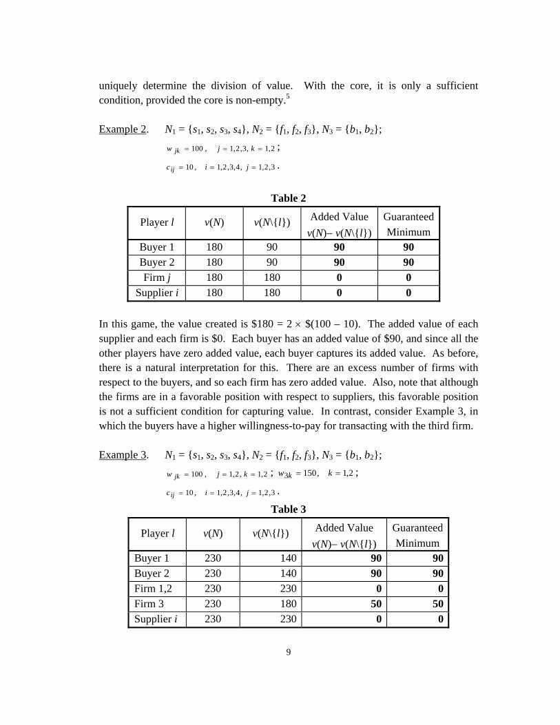
uniquely determine the division of value. With the core, it is only a sufficient condition, provided the core is non-empty.5 Example 2. N1 = {s1, s2, s3, s4}, N2 = {f1, f2, f3}, N3 = {b1, b2};

2,1,3,2,1,100 kjw jk ;

3,2,1,4,3,2,1,10 jicij .

Table 2

Player l v(N) v(N\{l}) Added Value

v(N) v(N\{l})

Guaranteed

Minimum Buyer 1 180 90 90 90 Buyer 2 180 90 90 90 Firm j 180 180 0 0

Supplier i 180 180 0 0

In this game, the value created is $180 = 2 $(100 – 10). The added value of each supplier and each firm is $0. Each buyer has an added value of $90, and since all the other players have zero added value, each buyer captures its added value. As before, there is a natural interpretation for this. There are an excess number of firms with respect to the buyers, and so each firm has zero added value. Also, note that although the firms are in a favorable position with respect to suppliers, this favorable position is not a sufficient condition for capturing value. In contrast, consider Example 3, in which the buyers have a higher willingness-to-pay for transacting with the third firm. Example 3. N1 = {s1, s2, s3, s4}, N2 = {f1, f2, f3}, N3 = {b1, b2};

2,1,2,1,100 kjw jk ; 2,1,1503 kw k ;

3,2,1,4,3,2,1,10 jicij .

Table 3

Player l v(N) v(N\{l}) Added Value

v(N) v(N\{l})

Guaranteed

Minimum Buyer 1 230 140 90 90 Buyer 2 230 140 90 90 Firm 1,2 230 230 0 0 Firm 3 230 180 50 50 Supplier i 230 230 0 0

10

The game in Example 3 has much in common with the game in Example 2. The number of each type of player remains the same, and the sum of the added values equals the total value created: the value created is $230 = $(150 – 10) + $(100 – 10); the added values of the suppliers, the first firm, and the second firm are each $0; the third firm has an added value of $50, and each buyer has an added value of $90. As in Example 2, this is an example of perfect competition. But, unlike Example 2, one of the firms has positive added value, which it captures.6 The source of this firm’s added value is that it is “different” from its competitors. That is, it has a favorable asymmetry between itself and the other firms. In this example, the favorable asymmetry takes the form of buyers having a higher willingness-to-pay for its product. In moving from Example 2 to Example 3, the third firm established positive added value through a favorable willingness-to-pay asymmetry. Alternatively, the third firm could have established positive added value through a favorable asymmetry on the supplier side. In such a case, the suppliers would have had a lower opportunity cost of providing resources to the third firm, as compared with providing them to the other two firms. In either case, a favorable asymmetry would have led to positive added value. This focus on favorable asymmetries as a source of added value can prompt some of the basic questions which a (potentially) profitable business would want to answer. These questions arise by performing the following thought experiment. Suppose, hypothetically, that a company were to close its business. If it has added value, it must be true that

(1) its buyers would then buy a product for which they had a lower willingness-to-pay (WTP) (or not buy at all), or

(2) its suppliers would incur a higher opportunity cost (OC) in supplying their resources to another business (or not supply at all), or

(3) both. The logic behind this thought experiment is implied by this informal question: If a company disappeared from the market, and its buyers wouldn’t care and its suppliers wouldn’t care, why would it be making any money? In other words, without a favorable asymmetry, why would the company capture any value? Testing for such a favorable asymmetry is what prompts the basic

11

business questions. For instance, the company should ask, if it were to disappear: Whom might its buyers buy from? Would its buyers have a lower WTP for this alternative? Why would its buyers have a lower WTP for this alternative? Whom might its suppliers sell to? Would its suppliers have a higher OC for this alternative? Why would its suppliers have a higher OC for this alternative? These questions, though seemingly straightforward, actually require a good understanding of a business to answer properly. In particular, notice that answers to these questions require that the company understand: who its buyers are, and why they might prefer its products; who its suppliers are, and why they prefer doing business with it; whom else its buyers might want to buy from; and whom else its suppliers might want to do business with. In short, the question of positive added value is the question of existence of a favorable asymmetry, which, in turn, is the question of whether a business is viable.

2. Choosing the Game

The previous section used the supplier-firm-buyer game to demonstrate how the structure of a business context could be modeled by a cooperative game. When using cooperative games, the term “structure” is well-defined: the players in the game and the value created by any group of these players. Therefore, whenever this structure is changed, the game also is changed. Thus, many a strategic decision is actually a decision about what game to be in. Examples include investing in a technology that reduces costs, finding ways to increase the willingness-to-pay for a product, changing production capacity, deciding to merge or integrate, and so on. In short, any decision that affects either the players in the game or the value created by any group of the players is a decision about choosing what business game to be in. This section discusses biform games. A biform game is a hybrid game form designed to model situations in which players can choose what business game to play. Roughly speaking, a biform game is a non-cooperative game in which the consequences are cooperative games rather than specific payoffs.

12

Following a description of the formalism, two applications of a biform game will be presented: a monopoly model and a spatial competition model. The Biform Formalism

The definition of a biform game starts with a strategic game form, that is: (1) a finite set N of players, and

(2) for each player i N, a set Ai of strategies.

Let iNi

AA . Consider:

(3) a function V : A N2 satisfying that for every a in A,

V(a)() = 0, and

(4) for each player i, a number i in [0, 1]. A biform game is then a collection NiiNii VAN }{;;}{; .

The formalism of a biform game may be interpreted as follows. The players first make strategic choices from the strategy spaces Ai. Each resulting profile a in A of

strategic choices induces a TU cooperative game V(a) : 2N , which is interpreted

as a business game. For each player i, the number i is termed player i’s confidence

index. When a player’s value-capture depends, partially or totally, upon a residual bargaining problem, the confidence index describes the extent to which player i anticipates that its appropriation of value will be in the upper, rather than lower, part of the residual problem. Similar to a strategic-form, non-cooperative game, players simultaneously choose strategies in a biform game. But the consequence of a profile of strategies is a cooperative game, not a vector of payoffs. The analysis of a biform game therefore requires the specification of each player’s preferences over different cooperative games. This specification is a three-step process, as described below. For every profile a in A of strategic choices and resulting TU cooperative game V(a),

(1) compute the core of V(a), and, for each player i N, (2) calculate the closed bounded interval of payoffs to player i delimited by

the core,7 and

13

(3) evaluate the interval as an i : (1 – i ) weighted average of the upper and

lower endpoints. As in the discussion of the supplier-firm-buyer game, unrestricted bargaining is assumed and modeled by either the added value principle or the core. Step 1 uses the core, and in Step 2, the residual bargaining problem is calculated. (If using the added value principle, the determination of each player’s range of possible value-capture replaces Steps 1 and 2.) The remaining task is to establish preferences over the residual bargaining problems for each player. This is Step 3.8 Notice that with Steps 1 through 3, the consequence of a strategy profile now reduces to a vector of payoffs. This allows a biform game to be analyzed as a strategic-form, non-cooperative game. A Monopoly Game9

A monopolist’s capacity decision is one of the simplest examples of a strategic decision affecting the structure of the game. The following example presents a basic monopoly situation, with one seller and a finite number of buyers. The player set N is {s, 1, 2, . . ., b}, where player s is the seller, and players 1, 2, . . ., b are the buyers. The seller is the only player with a strategic decision to make, namely how much capacity to install. Thus, the strategy set A is {0, 1, 2, . .}, with typical element a. The seller has a constant cost-per-unit for installing capacity, namely k, and, for simplicity, a zero cost-per-unit for producing its product. Each buyer has a willingness-to-pay for only one unit of product. For a given buyer, say j, its willingness-to-pay is denoted by wj, with w1 > w2 > . . . > wb > k > 0. The ordering

of the buyers in terms of descending willingness-to-pay is without loss of generality. The condition wb > k ensures that it is socially optimal to install capacity for all the

buyers. The characteristic function for this example is defined by

V(a)(S) = 0 if s S, –ka if S = {s}, (5)

–ka + Rj js wj1

)(I otherwise;

where

IS (j) = 1 if j S, (6)

0 otherwise;

14

R = max {r : rjjs1)(I < min{a, |S| – 1}}. (7)

Equations (5) through (7) merely state that if the number of buyers in a coalition exceed the capacity choice of the seller, then the buyers with the higher willingnesses-to-pay are assumed to be the ones who transact with the seller. Given this model, the question is: how much capacity will the seller choose to install? The answer to this question depends upon how much value the firm will capture for each possible capacity choice. Using the added value principle to model unrestricted bargaining, the following propositions determine the players’ value capture. (Brandenburger and Stuart (1996a) obtain the same results using the core. Their proof is easily adapted to prove the propositions below.) Proposition 1.1. Suppose a = 0. Then with the added value principle every player receives 0. Proposition 1.2. Suppose 0 < a < b. Then with the added value principle:

(i) player s receives between a(wa+1 – k) and

aj

j kw1

)( ;

(ii) player j (for j = 1, . . . , a) receives between 0 and (wj – wa+1);

(iii) player j (for j = a + 1, . . . , b) receives 0. Proposition 1.3. Suppose a > b. Then with the added value principle:

(i) player s receives between –ka and –ka + bj

jw1

;

(ii) player j (for j = 1, . . . , b) receives between 0 and wj.

To interpret these results, first suppose that the seller chooses capacity sufficient to serve every buyer. What value might the seller capture? One answer would be that it depends on the price the seller sets. But this answer assumes that the seller has price-setting power. What is the basis for this assumption? Or as Kreps (1990, pp. 314-315)asks: “[H]ow do we determine who, in this sort of situation, does have the bargaining power? Why did we assume implicitly that the monopoly had all this power (which we most certainly did when

15

we said that consumers were price takers)? Standard stories, if given at all, get very fuzzy at this point. Hands start to wave ...” Furthermore, why is it not true that the seller is involved with a collection of bilateral bargaining problems? If this is so, then the monopolist should not have any more power than the buyers. Proposition 1.3 implies just such a conclusion. If the monopolist has the capacity to serve the whole market, then it does not have any

inherent “monopoly power.” The cost of capacity, namely ka, is a sunk cost

incurred by the seller. The remaining value, namely bj jw1 , is the sum of residual

bargaining problems in which each buyer can capture between zero and its added value. With capacity to supply the whole market, a monopolist does not have any monopoly power. But with under-supply, Proposition 1.2 suggests a differ-ent story. For concreteness, consider the example depicted in Figure 2.

Figure 2

0123456789

1011121314

0 1 2 3 4 5 6 7 8 9 10 11 12 13

Quantity

B

A

16

In this example, there are 12 buyers with willingness-to-pays ranging from $13 down to $2. The per-unit cost of capacity for the seller is $1, and the seller has chosen a capacity of 9 units. The added value of the first buyer, the buyer with a willingness-to-pay of $13, is $9. (In Figure 2, the first buyer’s added value equals the shaded area.) Without this buyer in the game, the seller would instead transact with the just-excluded buyer, the buyer with a willingness-to-pay of $4. This would yield a loss in the value created of $9. Thus, the added value of the first buyer is $9, namely the value wj – wa+1 from part (ii) of Proposition 1.2. Notice what this implies for the

seller. When the first buyer transacts with the seller, $13 of value is created. Since the buyer cannot receive more than its added value, the firm is guaranteed to capture at least $4 of value, namely wa+1.

This reasoning can be repeated for the second through ninth buyers. From each buyer, the seller is guaranteed to receive at least $4 for a total of awa+1. Subtracting

out the cost of capacity, namely ak, yields the term a(wa+1 – k) in part (i) of

Proposition 1.2. Region A depicts this value. Region B depicts the residual value. Similar to the case of full market supply, the seller still faces a collection of bilateral bargaining problems. But with under-supply, the size of these bargaining problems has been reduced, and a minimum price has emerged. With no ex ante assumptions about price-setting power, the monopolist now has the power to receive a price of at least $4. With this model, the source of a monopolist’s bargaining power can be interpreted as competition provided by just-excluded buyers. By limiting capacity, the monopolist creates excluded buyers. The just-excluded buyer provides competition among the buyers, reducing the added values of the included buyers. The reduction in buyers’ added values guarantees value-capture to the firm, and a minimum price emerges. Proposition 1 characterizes the consequences of the seller’s capacity decision, but it does not identify the optimal choice of capacity. Due to the residual bargaining problems, the optimal choice will depend upon the seller’s confidence index.

Proposition 6.4 of Brandenburger and Stuart (1996a) shows that if = 0, the seller will choose a capacity equal to the quantity sold in a standard price-setting model. If

= 1, the seller will choose capacity to serve every buyer, namely the quantity in the classic case of perfect price discrimination. For values between these two extremes,

the optimal capacity choice is monotonically increasing in

17

A Spatial Competition Model10

The monopoly model provided an example of a biform game in which only one player had a strategic choice. In the spatial competition model that follows, there can be two or more firms, each having to make a strategic decision of where to locate. As in the monopoly example, buyers will be interested in obtaining only one unit of product. In this model, the player set is the union of two disjoint sets, a set F of firms and a set T of buyers. For non-triviality, there are at least two firms and two buyers. Only the firms have strategic choices. Each player Fi has a strategy set Ai and a confidence

index i. The sets Ai are compact, identical, and equal to a set 2R . Let

iFi

AA , with typical element Aa . The function V is defined by:

),(min))(( jiTj Fi

bacwNaV

, (8)

and for NS ,

),(min))(( jiTSj FSi

bacwSaV

(9)

if TSFS and , and

0))(( SaV . (10)

if TSFS or .

The function c is a differentiable function from 22 to }0{ .

An element Aa represents a choice of location for each firm. A given buyer, say j,

is located at position 2jb . Buyer j is willing to pay ),( ji bacw for the product

from firm i. The function c may be interpreted as the buyer’s transportation cost of transacting with the relevant firm. Thus, equations (8) and (9) state that the value created will be based upon each buyer purchasing from its “closest” firm, where the metric for “closeness” is transportation cost. Alternatively, each buyer may be interpreted as having a willingness-to-pay of w, with firm i incurring a cost of c(ai, bj) to provide buyer j with one unit of product. (The choice of interpretation will not affect the analysis.) For simplicity, the firms have no cost of production.

18

Furthermore, it is assumed that any firm could feasibly supply the whole market:

),( ji bacw for all ii AaTjFi ,, . There are no assumptions about the distribution

of the buyers, but since every firm is assumed to be able to supply all the buyers, the interpretation of the model is more reasonable if the distribution of the buyers is not too dispersed. With this model, the central question is: where should each firm choose to locate? Answering this question requires virtually the same approach as in the monopoly example. The consequences of different choices of location must first be characterized, with unrestricted bargaining in the resultant cooperative games modeled by the added value principle. Then, given these consequences, optimal choices of location can be identified. To analyze this biform game, it is convenient to define, given a profile of location choices, a buyer’s closest firm and a firm’s set of “local” buyers. For a given firm

Fi , let }}{\),(),(:{ iFkbacbacTjT jkjii denote its set of local buyers.

(These are the buyers for whom firm i is strictly closer.) Note that a set Ti may be

empty. For a given buyer Tj , let }:{ ij TjFiF denote the set containing the

buyer’s closest firm. Note that a set Fj is either a singleton set or the empty set.

Given an Aa , the following proposition characterizes the added value principle for the resultant cooperative game (V(a);N). Stuart (1998) proves a similar proposition using the core. Proposition 2. In the game (V(a);N), with the added value principle (i) a player Fk receives between 0 and

),(min),(min}{\

jiFi

jiTj kFi

bacbac

k

,

(ii) a player Tj receives between

),(min\

jiFFi

bacwj

and ),(min jiFi

bacw

.

Part (i) of this proposition states that the firm will capture an amount of value anywhere between zero and its added value. This added value is just its relative cost advantage with respect to its local buyers. (If a firm has no local

19

buyers, its marginal contribution equals zero, and so it receives nothing.) Part (ii) states that each buyer may also capture value up to its added value. But, unlike the firms, a buyer is guaranteed a minimum amount of value. This value is equal to its added value minus the incremental cost of transacting with its second-closest firm. If

a buyer does not have a unique, closest firm, i.e. Fj = , then the buyer is guaranteed its added value. As an example, Figure 3 depicts a two-firm case in which the buyers are uniformly distributed along a line. The horizontal axis represents location; the curve with the left-hand peak represents each buyer’s willingness-to-pay for firm one’s product; and the curve with the right-hand peak represents each buyer’s willingness-to-pay for firm two’s product. Region R1 depicts the added value of firm one.11 Without firm one, all the buyers would have to purchase from firm two, and the value created would correspond to regions R2 and R3. Region R1 must, therefore, be firm one’s added value. By symmetric reasoning, region R2 represents the added value of firm two.

Figure 3

To relate Figure 3 to Proposition 2, consider the buyer labeled j. From part (ii) of the

proposition, the value guaranteed to the buyer is w c(a2, bj), denoted by d2 in the figure. The existence of guaranteed value-capture suggests the presence of competition, and this is indeed the case. Since firm two has capacity to supply all the buyers, it will surely have an excess unit to

d 2

0.0

10.0

20.0

30.0

40.0

50.0

60.0

70.0

80.0

90.0

100.0

R1 R2

R3

d 1

j

20

sell to buyer j. Although buyer j will prefer to transact with firm one, firm two’s excess unit provides competition to firm one in its bargaining with buyer j. Further, since buyer j views firm two’s product as inferior (since it is farther away), it only guarantees that buyer j captures some of its added value. At the other extreme, buyer

j could capture up to its added value, w c(a1, bj), denoted by d1 in the figure. Part (i) of the proposition is almost immediate from part (ii). If each buyer captures its added value, the firms capture no value. If each buyer captures its minimum, then the

firms capture their respective added values. If the quantity d1 d2 is interpreted as a location advantage, then part (i) states that a firm may capture an amount ranging from zero to its relative location advantage. Proposition 2 states that a firm will receive between zero and its added value. Since a

firm evaluates this interval with an : 1 weighting, a given firm k will choose strategy ak equal to

),(min),(minmaxarg}{\

jiFi

jiTj kFi

kAa

bacbac

kkk

,

given a choice kk Aa by all firms }{\ kFi .

With this best response function, a solution for this biform location model can be characterized. Let ),(min),(min);(

}{\ji

Fiji

Tj kFikkk bacbacaaf

k

,

where a–k is taken to be fixed. Then the following proposition provides a solution.

Proposition 3. (Stuart 1998): Suppose k > 0 for all Fk . There exists Aa * such

that

(i) for all Fk , kkkkkk Aaaafaaf

);();( , and

(ii) AaNaVNaV ))(()*)(( .

This last proposition states that the biform location model has a solution (part (i)) and that there exists a solution which is socially optimal (part (ii)). Thus, with unrestricted bargaining, socially-efficient spatial differentiation can be an optimal strategy for the firms.

21

A partial intuition for this result can be gained from two observations. First, each firm wants to maximize its marginal contribution, namely its added value (Proposition 2). In many contexts, this condition is sufficient for a stable, socially-efficient outcome. Although this sufficiency does not hold in general, (see, for example, Makowski and Ostroy (1995)), it does hold in the biform location model. The reason is due to the second observation: there is a kind of independence in this model. Specifically, given a firm k, the value of the game without that firm, namely

}){\)(( kNaV , does not depend upon firm k’s choice of position. In other words, given

that all the other firms choose positions ak, }){\)(,( kNaaV kk has the same value for

all ak. With this sort of independence, individual maximization of added values will lead to social efficiency.

3. Conclusion

Cooperative game theory is a structural, rather than procedural theory. It does not specify what actions the players can take, much less what they might do. At first glance, this might seem disappointing for business strategy, since business strategy is often concerned with what a firm does. Instead, the structural approach of cooperative game theory can be used to answer a broader question: is the firm (or will it be) in a favorable competitive environment? Section 1 of this chapter demonstrates how cooperative game theory can be used to answer this broader question. It uses Supplier-Firm-Buyer games to model business games and gain insights into the nature of competition. Section 2 of this chapter addresses the “what might the firm do question.” Many business contexts are so complex that they resist specification of the players’ actions. But the choice of what business context to be in may be quite specifiable. Section 2 presents two examples of such choices: the capacity decision of a monopolist and the product positioning decisions of firms. Modeling these decisions does not, however, require that the structural approach of cooperative game theory be abandoned. Instead, the consequences of these decisions are complex business situations, which, with the biform game formalism, can be modeled as cooperative games. Thus, the answer to the “what might the firm do” question will be based on an assessment of how favorable a competitive environment the firm will find itself in.

22

References Aumann, R. (1985), “What is Game Theory Trying to Accomplish?” in Arrow, K. J. and S. Honkapohja (eds.), Frontiers of Economics, Oxford: Basil Blackwell, 28-76. Brandenburger, A., and H. W. Stuart, Jr. (1996), “Biform Games,” unpublished manuscript. Brandenburger, A., and H. W. Stuart, Jr. (1996), “Value-based Business Strategy,” Journal of Economics & Management Strategy 5, 5-24. Edgeworth, F. (1881), Mathematical Psychics. London: Kegan Paul. Hart, O. and J. Moore (1990), “Property Rights and the Nature of the Firm,” Journal of Political Economy 98, 1119-1158. Kreps, D. (1990), A Course in Microeconomic Theory. Princeton: Princeton University Press. McDonald, J. (1975), The Game of Business. New York: Doubleday. Makowski, L. (1980), “A Characterization of Perfectly Competitive Economies with Production,” Journal of Economic Theory 22, 208-221. Makowski, L. and J. Ostroy (1995), “Appropriation and Efficiency: A Revision of the First Theorem of Welfare Economics,” American Economic Review 85, 808-827. Milnor, J. (1954), “Games Against Nature,” in Thrall, R., C. Coombs, and R. Davis, eds., Decision Processes, New York: Wiley, 49-59. Osborne, and A. Rubinstein (1994), A Course in Game Theory. Cambridge: MIT Press. Oster, S.M. (1994), Modern Competitive Analysis. New York: Oxford University Press. Ostroy, J. (1980), “The No-Surplus Condition as a Characterization of Perfectly Competitive Equilibrium,” Journal of Economic Theory 22, 183-207. Roth, A. and X. Xing (1994), “Jumping the Gun: Imperfections and Institutions Related to the Timing of Market Transactions,” American Economic Review 84, 992-1044. Shapley, L. and M. Shubik (1972), “The Assignment Game, I: The Core,” International Journal of Game Theory 1, 111-130. Shubik, M. (1959) “Edgeworth Market Games,” in Tucker, A. W. and R. D. Luce, eds., Contributions to the Theory of Games, Vol. IV (Annals of Mathematics Studies, 40). Princeton: Princeton University Press, 267-278. Stuart, H. W., Jr. (1997), “Does Your Business Have Added Value?,” unpublished manuscript. Stuart, H. W., Jr. (1998), “Spatial Competition with Unrestricted Bargaining,” unpublished manuscript. Stuart, H. W., Jr. (1997), “The Supplier-Firm-Buyer Game and its m-sided Generalization,” Mathematical Social Sciences 34, 21-27.

23

Notes 1 John MacDonald, a contemporary of von Neumann, was arguably one of the first to appreciate the relevance of cooperative game theory to business. 2 Treating price as a consequence of the economic structure dates back at least to Edgeworth (1881). For a modern treatment and interpretation, see Makowski and Ostroy (1995). 3 Biform games are defined in Brandenburger and Stuart (1996a). Related approaches can be found in Hart and Moore (1990), Makowski and Ostroy (1995), and Roth and Xing (1994). 4 The material in this section is taken from Brandenburger and Stuart (1996b), Stuart (1997a), and Stuart (1997b). 5 This fact is a discrete version of results in Ostroy (1980). 6 See Makowski (1980) for a discussion of firm profitability under perfect competition. 7 Formally, the projection of the core onto the ith coordinate axis. 8 For an axiomatic treatment of this weighted average, see Proposition 5.1 of Brandenburger and Stuart (1996a). 9 This material is taken from Brandenburger and Stuart (1996a). 10 This material is taken from Stuart (1998). 11 The area of R1 only approximates firm one’s added value. It is not exactly equal due to the discreteness of the buyers.