cooperative communications - stanford universitywsl.stanford.edu/~ivanam/monograph.pdf ·...

Foundations and TrendsR© inNetworkingVol. 1, Nos. 3-4 (2006) 271–425c© 2007 G. Kramer, I.Maric and R. D. YatesDOI: 10.1561/1300000004

Cooperative Communications

Gerhard Kramer1, Ivana Maric2 andRoy D. Yates3

1 Bell Laboratories, Alcatel-Lucent, Murray Hill, New Jersey 07974,USA,[email protected]

2 Dept. of Electrical Engineering, Stanford University, Stanford, California94305,USA, [email protected]

3 WINLAB, Rutgers University, North Brunswick, New Jersey 08902,USA,[email protected]

Abstract

This article reviews progress in cooperative communication networks.Our survey is by no means exhaustive. Instead, we assemble a repre-sentative sample of recent results to serve as a roadmap for the area.Our emphasis is on wireless networks, but many of the results applyto cooperation in wireline networks and mixed wireless/wireline net-works. We intend our presentation to be a tutorial for the reader whois familiar with information theory concepts but has not actively fol-lowed the field. For the active researcher, this contribution should serveas a useful digest of significant results. This article is meant to encour-age readers to find new ways to apply the ideas of network cooperationand should make the area sufficiently accessible to network designersto contribute to the advancement of networking practice.

1Overview

1.1 Introduction

The classic representation of a communication network is a graph, asin Figure 1.1, with a set of nodes and edges. The nodes usually rep-resent devices such as a router, a wireless access point, or a mobiletelephone. The edges usually represent communication links or chan-nels, for example a fiber-optic cable or a wireless link. Both the devicesand the channels may have constraints on their operation. For example,a router might have limited processing power, or perhaps it can acceptdata from only a few of its ports simultaneously. A fiber-optic linkhas a limited bandwidth (which can be quite large!). A wireless phone,

Fig. 1.1 A network graph.

272

1.1 Introduction 273

Table 1.1 Device and channel properties.

Devices (Nodes) Channels (Edges)Wireline Constraints: Independent channels

– processing speed/energy No interference– input/output (ports) Limited bandwidth– delay Slow changes

Limited network knowledge Packet erasures

Wireless Constraints: Broadcasting– transmit energy Interference– processing speed/energy Noise– half-duplex Limited bandwidth– delay Slow or rapid changes

Limited network knowledgeLimited channel knowledge

on the other hand, has limited battery resources and likely wishes toconserve energy. A wireless link can have rapid time variations aris-ing from mobility and multipath propagation of signals. Some of theseproperties are collected in Table 1.1 and are described in more detail inthis text.

The purpose of a communication network is to enable the exchangeof messages between its nodes. These messages, as generated by anapplication, are organized into data packets. In the traditional modelof a network, the nodes operate as store-and-forward packet routersthat transmit packets over point-to-point links. However, this model isunnecessarily restrictive as it ignores two important possibilities:

• Node Coding: Nodes can combine, or encode, any of theirreceived information and symbol streams.

• Broadcasting: Nodes overhear the transmissions of othernodes from which they are not required to receive messages.

Node coding is possible in any network, while the ability to over-hear transmissions is a property of the physical communication chan-nel. In particular, wireless devices inherently broadcast information inthat a signal to a particular receiving node can be overheard by othernodes. Typically, the wireless nodes treat these overheard signals asinterference and the system provides mechanisms to mitigate this inter-ference. For example, many second generation cellular phones employcode division multiple access (CDMA) to permit signal decoding in

274 Overview

the presence of interference [185]. As a second example, 802.11× wire-less LANs employ a media access control (MAC) protocol that enablesnearby nodes to share the broadcast channel by taking turns trans-mitting. The goal of these multiple access strategies is to ensurethat communication over a link is reliable. A consequence is that theparadigm of a network as a set of point-to-point communication links isreinforced.

On the other hand, it has been understood in the information theorycommunity for over three decades that wireless communication from asource to destination can benefit from the cooperation of nodes thatoverhear the transmission. As these intermediate nodes may generatetransmissions based on processing of the overheard signals, the signalingstrategies go well beyond the inherent cooperation offered by nodes thatact as store-and-forward packet routers.

The relay channel [181] models this communication situation. Fun-damental coding strategies for the relay channel were developed in [33].The key idea was that the relay can use the overheard transmission fromthe source to form its own transmission that aids in decoding at thereceiver. These pioneering efforts focused on the simplest case of onesource, one destination, and one relay.

More recently, the seminal work of [4] has spurred progress in net-work coding. The connection between relaying and network coding isthat both approaches represent cooperative techniques. A node pro-cesses either received signals (in the case of relaying) or messages andencoded packets (in the case of network coding) based on the transmis-sions of multiple nodes. Although final capacity results remain elusive,it has become apparent that cooperative techniques using node codingand broadcasting offer significant improvements over traditional store-and-forward wireless networks with point-to-point links.

1.2 Networking Protocols

Advances in cooperative communication have focused on two goals:

• increasing the communication rates across the network, and• increasing the communication reliability in networks with

time varying channels.

1.3 Objectives and Outline 275

The advances are often demonstrated by mathematical (informationtheory) analyses of signaling strategies over models of communicationchannels. The signaling strategies typically involve coordinated trans-missions by multiple network nodes; but despite recent progress, thereremain significant barriers to applying these results to the developmentof practical network protocols.

For example, many information-theory results are based on asymp-totically large block lengths and usually ignore the overhead neededto set up and maintain coordinated transmissions. In practice, how-ever, and in particular for mobile wireless networks, the time varia-tions in the communication channels necessitate variations in the signal-ing strategies. The setup and maintenance signaling therefore becomesa recurring cost. We use the term network protocol for a set of dis-tributed algorithms executed by the network nodes that configure,execute, and reconfigure signaling strategies in response to temporalvariations. A cooperative network protocol must incorporate methodsso that recurring setup costs do not dominate the efficiency gains of acooperative signaling strategy.

Much of the value of networking is derived from the interconnectionof heterogeneous devices and systems. It is worthwhile to keep in mindthat the Internet is not so much a network as a network of networks.These interconnections of networks are made possible by designing pro-tocols based on abstract models, as in the layers of the OSI or TCP/IPnetwork protocol stacks [18]. In particular, a network protocol is morevaluable by providing a certain capability over a more generic networkabstraction, even if this is at the expense of reduced performance. Inthis context, the development of practical cooperative protocols will befacilitated by identifying the simplest possible abstractions of cooper-ative signaling strategies.

1.3 Objectives and Outline

This text reviews progress in cooperative communication networks. Oursurvey is by no means exhaustive. Instead, we assemble a representativesample of recent results to serve as a roadmap for the area. Our empha-sis is on wireless networks, but many of the results apply to cooperation

276 Overview

in wireline networks and mixed wireless/wireline networks. We intendour presentation to be a tutorial for the reader who is familiar withinformation theory concepts but has not actively followed the field. Forthe active researcher, we would like this contribution to serve as a usefuldigest of significant results.

We hope this text will encourage readers to find new ways to applythe fundamental ideas of network cooperation. We also hope we havemade the area sufficiently accessible to network designers to contributeto the advancement of networking practice.

Chapter 2 provides an overview of conventional communication andnetworking. This includes information-theoretic capacity definitions forthe point-to-point links that are the traditional basis for networks, aswell as key elements of the link and network layer protocols. Whilemuch or all of this material will be familiar to the reader, we includeit to provide contrast to the cooperative networks that follow. Chap-ters 3, 4, and 5 emphasize an information-theoretic treatment of thecapacity of cooperative networks. In particular, Chapter 3 providesbasic definitions, and a sampling of fundamental network models andcorresponding capacity results. Chapter 4 develops the key ideas ininformation-theoretic relaying and makes apparent how the methodsgo well beyond store-and-forward routing. Chapter 5 focuses on time-varying wireless networks and how they can be made more reliablethrough the use of cooperative diversity mechanisms. Finally, Chap-ter 6 investigates implementation aspects of these cooperative strate-gies, concluding with a review of recent proposals in the literature fornetwork cooperation protocols.

2Conventional Networks: A Review

Before describing cooperative protocols and networks, we start witha review of networking models and common practices. Our discussionintroduces the conventional decomposition of a network into protocollayers. We then employ these layers to organize the subsequent review ofthe physical, link, and network layer protocols. We recognize that futurecooperative networks will also demand a re-examination of transportlayer protocols; however, we omit a review of the higher layers as theyare beyond the scope of this text. While much or all of this material islikely to be familiar, this review will serve as a baseline for comparisonswith cooperative networks.

2.1 Network Layering

Layering as embodied in the protocol stack of Figure 2.1 is a key ideain the development of networks. The stack of boxes (modules) arrangedas layers represents a network node. Each module operates at a partic-ular layer. The horizontal dashed arrows between modules in differentnodes signify that a module may exchange messages with its peer mod-ules in other network nodes. Messages that are sent through lower layer

277

278 Conventional Networks: A Review

Application

Network Network

Session Session

Presentation Presentation

Application Application

PhysicalInterface

PhysicalInterface

Data Link

Media Access Control

Data Link

Media Access Control

Transport Transport

PHY

IP

TCP

Wireless Channel

Fig. 2.1 Network protocol stack.

modules to peer modules in other network nodes are the basis for dis-tributed network algorithms.

Data packets are used to communicate from a source node to a des-tination node via a path with intermediate nodes. At the source, datapackets generated by an application are passed from module to mod-ule down through successive layers of the protocol stack. Each moduletypically appends its own header to each such data packet. A modulemay repackage the data packets, by dividing packets into smaller pack-ets. The packet headers serve as protocol signaling for peer modules,either at intermediate nodes or at the destination node. A module alsomay inject its own control packets in order to communicate with peermodules.

When a packet proceeds through a multihop route to a destination,a packet climbs no higher than necessary in the protocol stack. Thatis, a packet passing through an intermediate node will reach the net-work layer where the routing algorithm will decide to what node thepacket should be forwarded. Thus a packet reaches the transport layerand application layer only at the destination. At the destination, eachmodule is responsible for undoing the repackaging of its source node

2.1 Network Layering 279

peer by stripping the additional headers and control packets injectedby its peer. That is, the higher layer packets passed down to a moduleat the source should be passed back up to the higher layer module atthe destination.

In traditional wireline or wireless networks, these modules are welldefined. Packets are buffered and sequenced by the transport layer,typically TCP, that implements both a reliable end-to-end connectionas well as end-to-end flow control. Finding routes (via a sequence oflinks) to a destination is the job of the network layer. Maintainingthese routes and forwarding packets along these routes is also a networklayer task. The link layer ensures reliable packet communication on asingle link. As shown in Figure 2.1, this may include a MAC sublayerthat regulates channel access. The physical (PHY) layer represents thehardware that performs transmission and reception.

In an IP network, the full stack has the simplified representationshown in the gray boxes. In a wireless setting, the MAC sublayer, thelink layer, and the PHY layer are lumped together as a PHY layer.This combined PHY layer is just an interface queue that accepts IPpackets.

For our purposes, we start with a source node s running an appli-cation layer process that wishes to transmit messages to an applicationlayer process at a destination node t. The messages are encoded asdata packets with appropriate headers that identify the applicationprocess, the source node s and the destination node t. When thesepackets are passed to a TCP transport layer, sequence numbers areappended and the release of packets to the network layer is controlledby reverse stream of TCP ACKs from the receiver TCP process. Thenetwork layer examines the destination address (an IP address) anddetermines where to send the packet using a routing table. For exam-ple, the routing table for a source node attached to an Ethernet mightspecify only two rules: direct transmission to destination nodes on thesame Ethernet and forwarding to a gateway node for all other packets.

At the data link layer, it is common practice to append a cyclicredundancy check (CRC) to each packet. The CRC allows the data linklayer at the receiver to detect packet reception errors. Sequence num-bers may also be added to facilitate automatic repeat request (ARQ)


retransmission protocols at the link layer. The PHY layer is respon-sible for the transmission of bits to a receiver of a link. The codingand modulation employed at the PHY layer for a single point-to-pointlink may be quite complex. When forward error correction (FEC) andhybrid ARQ protocols are employed, the line between the physical andlink layers is blurred. However, above the link layer, one can assumethat the interfaces between layers are based on binary data packets.

In the following sections of this chapter, we climb the protocol stackin describing the traditional functions of the physical, link and networklayers.

2.2 Physical Layer: Communication Theory

We review basic concepts of communication theory. This theory is use-ful for all network layers, but in particular for the PHY and applicationlayers where source and/or channel coding are used. The following sec-tions also introduce notation that we use throughout the document.

2.2.1 Information Theory

Information theory began as the mathematics of communications forone source and one channel [164]. Consider Figure 2.2 and supposethe source puts out a message W that consists of B independent anduniformly distributed bits. Let X and Y be random variables repre-senting the channel input and output with alphabets X and Y, respec-tively. A discrete memoryless channel (DMC) is a conditional probabil-ity distribution PY |X(·), where X and Y are discrete and finite.1 Theencoder transmits a string Xn = X1,X2, . . . ,Xn that is a function of W .

SourceMessage

Channel

SinkDecoderEncoder

Fig. 2.2 Communications model.

1 The theory generalizes to continuous random variables in natural ways.

2.2 Physical Layer: Communication Theory 281

The decoder sees Y n = Y1,Y2, . . . ,Yn and puts out a message estimateW that is a function of Y n.

The capacity is the maximum rate R = B/n bits per channel usefor which, for sufficiently large n, there exists a W -to-Xn mapping(an encoder) and a Y n-to-W mapping (a decoder) so that the errorprobability Pr[W �= W ] can be made as close to 0 as desired (but notnecessarily exactly 0). It is a remarkable fact that such a capacityexists. Perhaps just as remarkably, the capacity is given by the compactformula

C = maxPX(·)

I(X;Y ) bits/use, (2.1)

where

I(X;Y ) =∑

a∈X , b∈Y,PXY (a,b)>0

PXY (a,b) log2PXY (a,b)

PX(a)PY (b)(2.2)

is the mutual information between X and Y . The formula (2.1) is uni-versal in the sense that it gives the capacity for any DMC. Furthermore,the capacity proof is based on a random code construction method thatis useful for many other communication problems [34, 35].

Similarly, consider the additive white Gaussian noise (AWGN)channel

Y =h

dα/2 X + Z (2.3)

with power constraint

n∑i=1

E[|Xi|2]/n ≤ P, (2.4)

where X and Z are real random variables; Z has variance N ; h, d,and α are real numbers; and E[·] denotes expectation. The variables h

and d represent channel gains and distances between the encoder anddecoder, respectively, and α is an attenuation exponent (e.g., α = 2 forfree-space propagation). The model (2.3) is not accurate for small d. Forexample, as d approaches zero, we have the physically untenable resultthat the received power exceeds the transmitted power. However, we


will be mainly interested in “long-range” communication where (2.3) isa reasonable model for distance-dependent attenuation. The capacityformula (2.1) generalizes in a straightforward way to AWGN channels,namely

C = maxpX(·)

∫pXY (a,b) log2

pXY (a,b)pX(a)pY (b)

dadb bits/use, (2.5)

where pXY (a,b) is the joint probability density of X and Y (if X is dis-crete, then replace pX(a) and pXY (a,b) by PX(a) and PX(a)pY |X(b|a),respectively, and replace the integral over X by a sum). The maximiza-tion in (2.5) is interpreted as constraining pX(·) to satisfy (2.4). Themaximum entropy theorem [34, p. 234] establishes that the best X isGaussian with zero mean and variance P , and the capacity is

C =12

log2 (1 + γ) bits/use, (2.6)

where

γ =(

P

N

) |h|2dα

(2.7)

is the signal-to-noise ratio (SNR) [34, p. 241]. Suppose next that X,h, and Z = ZR + jZI are complex with j =

√−1, and ZR and ZI areindependent, real, Gaussian random variables with variance N/2. Thecapacity is now

C = log2 (1 + γ) bits/use. (2.8)

2.2.2 Modulation

Consider the AWGN channel (2.3) with complex symbol alphabets. Letthe SNR in decibels be

γdB = 10log10 γ dB (2.9)

so that we can write the capacity (2.8) as

C = log2

(1 + 10γdB/10

)bits/use. (2.10)

We plot (2.10) in Figure 2.3 as the curve labeled “Gaussian.”


−10 −5 0 5 10 15 200

0.5

1

1.5

2

2.5

3

3.5

γdB

[dB]

C[bits/use] Gaussian

BPSK

3−PSK

QPSK

8−PSK

Fig. 2.3 Capacity of M -PSK signal sets.

The formula (2.10) is based on using X = XR + jXI , where XR

and XI are independent, real, zero-mean, Gaussian random variableswith variance P/2. However, for practical reasons such as amplifier con-straints, receiver synchronization, and detector complexity, one usuallyrestricts attention to X with a limited number of values. For exam-ple, for wireless communication one might restrict attention to M -aryphase-shift keying (M -PSK) where X is uniform over the alphabet

X ={√

Es,√

Esej 2π/M , . . . ,

√Ese

j 2π(M−1)/M}

, (2.11)

where Es = P is the (average) per-symbol-energy. The set X is calledthe signal set or the modulation set (cf. [148, Ch. 4]).

The capacity of the complex AWGN channel with M -PSK is(see (2.5))

C = − log2(πe) −∫

pY (b) log2 pY (b) db bits/use, (2.12)


where

pY (b) =M−1∑m=0

1M

pY |X(b |√

Esej 2πm/M

)(2.13)

and

pY |X(b|a) = pZR(�{b} − �{a}) pZI

(�{b} − �{a}) , (2.14)

where ZR and ZI are independent, Gaussian, and have variance N/2,and �{x} and �{x} are the respective real and imaginary parts of x.Suppose we use M = 2,3,4,8, whose signal sets are called binary PSK(BPSK), 3-PSK, quaternary PSK (QPSK) and 8-PSK, respectively.The capacities are plotted in Figure 2.3 as a function of γdB. Observehow the M -PSK capacities saturate at log2(M) bits/use at large γ.Clearly, at high SNRs one must use large signal sets, while at lowSNRs it seems that BPSK suffices (however, see the next sections onspectral efficiency).

Finally, we remark that the capacity calculations in this chapterassume that the receiver can accurately estimate the channel SNR.If this is not the case, then many interesting issues arise [184]. Forinstance, an important practical issue is the choice of signal set for thebest capacity scaling behavior at low and high SNRs [115, 117].

2.2.3 Spectral Efficiency

We next include the effect of bandwidth. Loosely speaking, the spectralefficiency of a modulation set is the number of bits per second per Hertzthat the set can support. To define spectral efficiency more precisely,we follow an approach similar to [165, Sec. VIII] and [188, Sec. 7.2] andmake the following idealizations:

(i) The channel passes frequencies f in the range

f0 − W/2 < |f | < f0 + W/2, (2.15)

where the center frequency f0 is much larger than W .2 Theequivalent baseband representations of the channel input and

2 Note that W is here the bandwidth rather than a message.


output signals are therefore complex and band-limited to|f | < W/2. We say that the channel bandwidth is W .

(ii) The channel is used for a period of T seconds. We describethe channel input and output signals by n = TW complexsamples spaced Ts = 1/W seconds apart, i.e., we can recon-struct the baseband input signal X(t) as

X(t) =n∑

i=1

Xi · sin(πWt − πi)πWt − πi

, (2.16)

where Xi is a complex number whose squared amplitude andphase are the respective energy and phase of the ith inputsample. The average energy per sample is

Es =n∑

i=1

E[|Xi|2

]/n. (2.17)

We consider primarily Gaussian signaling for which Xi is acomplex Gaussian random variable, or PSK for which |Xi|2 =Es for all i.

(iii) The channel adds complex Gaussian noise with power N toeach input sample, i.e., the ith channel output sample isYi = Xi + Zi where Zi = ZR,i + j ZI,i and ZR,i and ZI,i areindependent, Gaussian random variables each having vari-ance (N Ts)/2. Usually N increases proportionally with W ,and we write N = WN0 where N0/2 is the noise power perHertz.

The modulation rate is Rmod = log2(M) bits, where M is the num-ber of values that X takes on. For instance, QPSK has Rmod = 2bits. Suppose the encoder maps blocks of kc bits to blocks of nc bitsat the rate Rc = kc/nc. The overall coded modulation rate is there-fore R = RcRmod bits. The energy consumed per information bit isEb = Es/R and we define the information bit SNR ratio as Eb/N0. LetPb be the decoder bit-error probability.

It is now natural to define the spectral efficiency of the modulationat the bit-error probability Pb as

η(Eb/N0,Pb) = R∗cRmod bits/s/Hz, (2.18)


where R∗c is the maximum code rate for which one can achieve a bit-

error probability of Pb when the information bit SNR ratio is Eb/N0.For wireless transmission Pb can be 10−6, while for optical transmissionPb can be required to be 10−15 or less. However, one usually considersonly the case Pb → 0 because the spectral efficiency hardly changesas long as Pb ≤ 10−3. We denote the resulting spectral efficiency byη(Eb/N0).

Note that (2.18) defines spectral efficiency without taking intoaccount the spectral guard bands that are necessary in practice. Thereason for doing this is that the amount of guard band needed, in pro-portion to the bandwidth, will depend primarily on the pulse shape,and less on the number of points in the signal set. We will not considerpulse shaping.

2.2.4 Computing Spectral Efficiency

Recall that we use the channel n = TW times over T seconds, and thatthe channel is memoryless. The capacity normalized by the time andbandwidth is therefore (see (2.1))

C =maxPXn (·) I(Xn;Y n)

TW=

maxPX(·) I(X;Y )(T/n)W

bits/s/Hz. (2.19)

Let Ts = T/n be the symbol time. We are using Ts = 1/W so thedenominator of (2.19) is simply one. We further define Es = P Ts

and Ns = N Ts to be the transmit-symbol and noise-symbol energies,respectively. The mutual information in (2.19) is in general some func-tion of P/N = Es/Ns, i.e., we have

C = f(Es/Ns) = f (R · Eb/N0) , (2.20)

where f(·) is some non-decreasing function, and where we have usedEs = REb and Ns = N0(WTs). Note further that R ≤ C, so thatC ≤ f(C · Eb/N0) and, given Eb/N0, the “best” C is the largest C∗

satisfying

C∗ = f (C∗ · Eb/N0) . (2.21)


Equation (2.21) gives the ultimate Eb/N0 in terms of C∗, or the ulti-mate C∗ in terms of Eb/N0. We thus have

η(Eb/N0) = C∗ bits/s/Hz. (2.22)

For example, suppose we wish to compute η(Eb/N0) when arbitrarycomplex X are permitted. Since Rmod is in principle infinite here, onenow maximizes the overall rate R without separating it into Rmod andRc. We thus have

C = log2 (1 + Es/Ns) bits/s/Hz. (2.23)

We set Es = REb, Ns = N0, and use (2.23) and R ≤ C to obtain

2η − 1η

≤ Eb

N0. (2.24)

The η which satisfy (2.24) with equality are given by the curve labeled“Gaussian” in Figure 2.4, where (Eb/N0)dB = 10log10 Eb/N0. Observethat as η → 0 we have Eb/N0 → ln(2) ≈ 0.6931 which is −1.59 dB.

−2 0 2 4 6 8 100

0.5

1

1.5

2

2.5

3

(Eb/N

0)dB

[dB]

η[b/s/Hz]

Gaussian

BPSK

3−PSK

QPSK

8−PSK

Fig. 2.4 Spectral efficiencies for M -PSK.


The other curves in Figure 2.4 are those for M -PSK with M =2,3,4,8. Note the striking differences between Figures 2.4 and 2.3 at lowSNRs. Note also that at (Eb/N0)dB ≈ −1.59 dB we have that 3-PSK,QPSK, and 8-PSK all outperform BPSK by a factor of two in rate,but they perform just as well as Gaussian signaling. Thus, BPSK isinefficient at low SNRs, but 3-PSK and QPSK are practically optimal(cf. [183]).

2.2.5 Multi-Antenna Communication

The information theory developed above applies as well to multi-antenna communication. We model such problems by making the chan-nel inputs and outputs vectors, i.e., we have

Y =H

dα/2 X + Z, (2.25)

where X, Y , and Z are complex column vectors of length nX , nY , andnY , respectively, and H is a complex nY × nX matrix. The additivenoise vector Z has independent, Gaussian, entries with independentreal and imaginary parts with variance N/2 each. The block powerconstraint is now

n∑i=1

E[‖Xi‖2]/n ≤ P, (2.26)

where ‖X‖2 = X†X and X† is the complex-conjugate transpose of X.One can show that the best X are zero-mean and Gaussian by the

maximum entropy theorem [34, p. 234]; we write the covariance matrixof X as QX = E[X X†]. The capacity is (see (2.1))

C = maxpX(·)

I(X;Y ) (2.27)

= maxQX

log∣∣∣∣I +

1dαN

HQXH†∣∣∣∣ , (2.28)

where (2.28) follows by [34, Thm. 9.4.1], |A| is the determinant of A, andwhere the maximizations in (2.27) and (2.28) are interpreted as con-straining pX(·) to satisfy (2.26). Consider the matrix H and recall thatwe can use the singular value decomposition to write H = V ΣU † whereU and V are unitary and Σ is a nY × nX matrix that is zero except

2.3 Link Layer: ARQ and HARQ Protocols 289

for the (non-negative) singular values on the diagonal [75, p. 414]. Wethus have

C = maxQX

log∣∣∣∣I +

1dαN

ΣQXΣ†∣∣∣∣ , (2.29)

where we have used |V | = 1 and V †V = I to remove the V [75, p. 414],and where we have included the U in the optimization of QX .

The resulting optimization problem is the same as for parallel Gaus-sian channels [34, p. 250]. The optimal QX for this problem is known tobe diagonal with entries Pi = E[|Xi|2], i = 1,2, . . . ,nX , chosen accord-ing to a “waterfilling” solution. More precisely, if we let σi be the ithdiagonal entry of Σ, we choose Pi to satisfy

Pi =

{max

(Q − N

σ2i,0)

if σi �= 0,

0 otherwise(2.30)

where the “water level” Q is chosen so thatnX∑i=1

Pi = P. (2.31)

2.3 Link Layer: ARQ and HARQ Protocols

For the PHY layer, error control is usually based on both AutomaticRetransmission ReQuest (ARQ) and FEC schemes (“forward” refersto the non-feedback aspect of error control where a code automaticallycorrects errors detected at the receiver). ARQ is a link layer protocolthat provides reliability based on error-detecting codes and retransmis-sions. A parity-bit or CRC check of a received packet triggers retrans-mission requests. If the receiver determines that the packet is in error,it sends a negative acknowledgment (NAK) to the transmitter, oth-erwise it sends an acknowledgment (ACK). In the former case, thepacket is retransmitted. From the perspective of the application layer,such retransmissions are Automatic (the acronym ARQ is based onthe Morse designation for retransmission request [52]). Some flavors ofthis protocol include stop-and-wait [186], go-back-N [17], and selective-repeat [121], and they each provide different tradeoffs in throughputand buffering at the transmitter and/or receiver.


The throughput of ARQ protocols can be improved by combiningFEC with ARQ in the form of Hybrid-ARQ [31, 120]. Hybrid-ARQ letserroneous received packets be collected and combined in various waysbefore decoding. One can exploit this idea for cooperative communi-cation as well, and we address such protocols in detail in Chapter 6.Packet combining can be based on hard decisions or soft channel out-puts. In the latter case, noisy versions of the same packet are combinedby maximal-ratio, equal gain, or selection combining diversity tech-niques. The transmitted packets can thus be viewed as symbols of arepetition code, and this idea can be extended to more general classesof codes. As another approach, incremental redundancy ARQ can berealized with rate compatible punctured convolutional codes (RCPC)by first using the highest rate code from the RCPC code family andsending additional bits as needed [67]. Alternatively, with turbo codesone punctures parity bits [141].

2.4 Network Layer: Wireless Routing Protocols

The role of the network layer is to route packets to their intendeddestinations. In a traditional network, a node implements a routingtable that maps the destination address of a packet to a rule for for-warding that packet. In a wired network, the routing table specifies theoutgoing link on which to forward a packet. In a wireless network inwhich the physical medium is a broadcast channel, the routing tablemay specify the intended next recipient of a packet.

In wired networks, link topology changes are infrequent and routingtables tend to be fairly static. This is reinforced by the use of policy-based routing in which the routing of packets depends on negotiatedagreements among the operators of autonomous systems [51].

By contrast, wireless networks enable node mobility which caninduce a stochastic process of link connection and disconnection. Inresponse, mobile ad hoc networks implement specialized routing algo-rithms in the network layer [88, 147] that adapt to these frequent topol-ogy changes. These routing algorithms have been the starting point formobile networking research. Changes in wireless link topology result infrequent routing table updates and necessitate distributed algorithms

2.4 Network Layer: Wireless Routing Protocols 291

for route discovery and route repair, as well as appropriate metrics forchoosing efficient routes.

In the mobile networking community, Dynamic Source Routing(DSR) [88] and Ad hoc On-demand Distance Vector (AODV) [147]routing have emerged as de facto standards for mobile network routing.Each has open-source implementations for linux [30, 42, 129, 155] andthe ns-2 simulator [8, 21, 130, 177]. Both protocols implement routediscovery, route caching, and route maintenance in response to timevariations in link connectivity. The protocols differ in how the rout-ing information is stored. Here we describe these protocols in detailto convey the complexity of the task, even if the network is limitedto store-and-forward operations. We start with DSR and then describehow AODV differs.

2.4.1 DSR

DSR is a source routing protocol that adds to each data packet a headerspecifying the complete route (a sequence of nodes) that the packetmust follow to the destination. Each mobile node maintains a cachethat holds source routes that it has learned. When a node wants tosend a packet to another node, it first checks its route cache for asource route to the destination. If no route is found, the source willinvoke the route discovery procedure.

A node initiating route discovery (called the initiator) broadcasts aroute request (RREQ) packet which may be received by those nodeswithin range. The RREQ packet identifies the intended destination,referred to as the target node and contains a unique request id set bythe initiator from a locally maintained sequence number. In additionto the addresses of the initiator and target of the request, each RREQpacket contains a route record, the accumulated sequence of hops takenby the RREQ packet as it is forwarded.

When a node receives a RREQ packet, it processes the requestaccording to the following steps:

• If the pair (initiator address, request id) of the RREQ packet isfound in this node’s list of recently seen requests, the request


is discarded. This removes later copies of the request thatarrive at this node by alternate routes.

• If this node’s address is already in the route record, theRREQ packet is discarded. This guarantees that no singlecopy of the request can propagate around a loop.

• If the target of the request matches this node’s own address,then the route record contains the route from the initiator bywhich the request reached this node. In this case, this nodereturns a copy of this route in a route reply (RREP) packetto the initiator.

• If this node has a route cache entry for the target, it appendsthis cached route to the accumulated route record in thepacket, and returns this route in a RREP packet to the ini-tiator without re-broadcasting the RREQ.

• Otherwise, this node appends its own address to the routerecord in the RREQ packet, and re-broadcasts the request.

The RREQ thus propagates through the ad hoc network until itreaches the target host, which then replies to the initiator. Effectively,route discovery is implemented by controlled flooding of the RREQpacket. If the route discovery is successful, the initiator receives a RREPpacket listing a sequence of network hops through which it may reachthe target.

In conventional routing protocols, nodes exchange periodic rout-ing updates. If the status of a link or a node changes, the periodicupdates eventually reflect the changes to all other nodes, resulting inthe computation of new routes. However DSR does not have peri-odic messages of any kind from any of the mobile nodes. Instead,while a route is in use, the route maintenance procedure monitorsthe operation of the route and informs the source of any routingerrors.

Since wireless links are generally less reliable than wired links, manywireless networks, including 802.11, utilize a hop-by-hop acknowledg-ment at the data link layer in order to provide early detection andretransmission of lost or corrupted packets. In these networks, routemaintenance can be easily provided, since over each link, the transmit-


ting node can determine if the link is up. If the data link layer reportsan unrecoverable transmission problem, the transmitting node sends aroute error (RRER) packet to the original source of the packet. TheRRER packet contains the addresses of the nodes at both ends of thelink in error. When a RRER packet is received, the link in error isremoved from this node’s route cache, and all routes that contain thislink are truncated.

We note that a node can add entries to its route cache whenever itlearns a new route. In particular, when a node forwards a data packetas an intermediate link on the route in that packet, the forwardingnode is able to observe the entire route in the packet. If a node for-wards an RREP packet, it can also add the route information fromthe route record being returned in that route reply, to its own routecache. Finally, since all wireless network transmissions are inherentlybroadcast, a node may be able to configure its network interface intopromiscuous receive mode, and can then add to its route cache theroute information from any overheard data or RREP packet.

In order to return the RREP packet to the initiator of the routediscovery, the target reverses the route in the route record from theRREQ packet, and use this route to send the RREP packet. This,however, requires the wireless network communication between eachof these pairs of hosts to work equally well in both directions, whichmay not be true in some environments or with some MAC-layerprotocols.

2.4.2 AODV

AODV uses a broadcast route discovery mechanism, as is also usedby DSR. Instead of source routing however, AODV relies on dynami-cally establishing route table entries at intermediate nodes. This differ-ence pays off in networks with many nodes, where a larger overhead isincurred by carrying source routes in each data packet. AODV uses des-tination sequence numbers, as in destination-sequenced distance-vector(DSDV) routing [146], to maintain the most recent routing informa-tion. Each node maintains a monotonically increasing sequence num-ber which is used to supersede stale cached routes. AODV also features


timer-based states in each node. A routing entry is deleted if not usedduring a specific amount of time.

Route discovery in AODV is very similar to DSR. The main differ-ence is the use of sequence numbers. In addition to the similar fields inthe DSR RREQ, the AODV RREQ contains the pair (source sequencenumber, last destination sequence number known to the source). Thesource sequence number is used to maintain freshness informationabout the reverse route to the source and the destination sequencenumber specifies how fresh a route to the destination must be in orderto be accepted by the source.

As the RREQ is flooded, it automatically sets up the reverse pathfrom all nodes back to the source. To set up a reverse path, a noderecords the address of the neighbor from which it received the firstcopy of the RREQ. These reverse path route entries are maintainedlong enough for the RREQ to traverse the network and produce areply to the source.

When an RREQ arrives at a node (possibly the destination itself)that has a routing table entry for the destination, it checks the fresh-ness of that entry by comparing the destination sequence number ofthe route entry with that in the RREQ. If the sequence number ofthe RREQ is strictly greater, the routing table entry cannot be usedto respond to the RREQ; instead, the node rebroadcasts the RREQ.Otherwise, if the RREQ has not been processed previously, the nodethen unicasts a RREP packet back to the sender of the RREQ. As theRREP travels back to the source, each node along the path sets upa forward pointer to the node from which the RREP came, updatesits timeout information for route entries to the source and destination,and records the latest destination sequence number for the requesteddestination.

A node receiving an RREP propagates the first RREP for a givensource node toward that source. If further RREPs are received, thenode updates its routing information and propagates the RREP only ifthe RREP contains either a greater destination sequence number thanthe previous RREP or the same destination sequence number with asmaller hop count.


When a link fails, the node upstream of the break sends a RRERpacket with a fresh sequence number (i.e., a sequence number that isone greater than the previously known sequence number) and a hopcount of infinity to all active upstream neighbors. Then these nodesrepeat the same process and so on. This process continues until allactive source nodes are notified and then terminates because AODVmaintains only loop free routes and there are only a finite numberof nodes in the network. We note that this is unlike DSR in whichbroken link information may not be propagated to all route cacheswith that link.

2.4.3 Properties of Ad Hoc Routing Algorithms

It is important to note that the DSR and AODV algorithms are basedon IP packets. Logically, mobile ad hoc IP networks differ from ordinaryIP networks only in the network layer. In particular, the model abstrac-tion of point-to-point links is preserved; only link state (up/down)changes become more frequent. The cooperation between nodes is lim-ited strictly to packet store-and-forward. Despite this relative simplic-ity, the deployment of ad hoc routing at all nodes in a mobile wirelessnetwork results in a network with a very large state space. Whether inthe form of a DSR cache or an AODV routing table, every node main-tains its best guesses regarding available routes. As mobility causes linktopology changes, these guesses will be outdated and likely have con-flicts from node to node. As a result, the analysis of routing algorithmsin mobile environments can do little more than verify correctness inquasistatic environments.

Instead, a large literature of experimental evaluation has emerged.Much of this is simulation-based [21, 38, 74, 130, 155, 194] but therehas also been testing with small networks of nodes and 802.11 radiointerfaces [95, 131, 142]. Much of this mobile ad hoc routing literaturehas focused on certain fundamental problems. In particular, route dis-covery and route maintenance generate a flurry of packets and unnec-essary route discovery should be avoided [21, 38, 155]. On the otherhand, when mobility induces link failures, fast route maintenance anddiscovery are vital. In addition, there are non-trivial cross-layer inter-


actions between the MAC, the routing protocol and the transport layer[140, 142]. For example, excess consumption of bandwidth resources byTCP can cause congestion in the 802.11 CSMA protocol, which cancause route maintenance to be invoked [140].

Additional issues arise with interactions with transport layer proto-cols. Consider an 802.11 ad hoc wireless network with stationary nodessuch that the PHY layer radio connectivity is adequate. Suppose thatthese nodes are supporting a TCP file transfer over a multihop radiopath. In this case, data packets in the forward direction (from senderto receiver) contend for the channel with RTS/CTS messages at thePHY layer as well as with TCP ACK messages in the reverse direction.These contending data packets cause self interference to the multihoproute and can disrupt timely control message exchanges. This conditioncan be perceived as a link failure, triggering inappropriate route repairor route discovery mechanisms, ultimately resulting in transport layertimeouts and dramatic reductions in throughput [64]. This deficiencyis in addition to the problems caused by PHY layer outages inducedby fading on a single link, for which transport layer solutions [15, 16]have been developed.

Finally, we recall that DSR and AODV were designed to use onlyIP packets. As a result, simple hop metrics are the primary basis forrouting. Frequently, the fastest route reply is equated with the bestroute. When links have variable rates, this is not necessarily correct.Since the RREQ and RREP packets are small, they travel faster acrosslong distance hops at lower communication rates. Moreover, in an802.11 environment which employs uncoded packets, these short con-trol packets can be received on marginal links that are useless for longerdata packets. Thus, longer data packets generally benefit from routeswith shorter-distance higher-data-rate links. MAC-layer and network-layer enhanced routing algorithms have emerged to address such issues[13, 39]. We will see that these approaches have analogies to the coop-erative approaches described in Chapter 6.

3Network Models

The aim of this chapter is to develop a common framework for analyzingcapacities of wireline and wireless networks. Our focus will, in fact, beon physical- and link-layer issues for wireless problems. However, thereare close relations between wireline and wireless networks that we wishto highlight, and that we hope will lead to a better understanding ofboth types of networks.

As is customary, we will represent a network by a graph, i.e., a setN of nodes and a set E of edges that are pairs of nodes (see Figure 1.1).If an edge (u,v) is directed, then the ordering tells us that the edge goesfrom node u to node v. For example, the directed network in Figure 3.1below has N = {1,2,3} and E = {(1,2),(2,3)}.

3.1 Wireline Network Models

The channels (or edges) of a wireline network are usually modeled asbeing independent in the sense that the signals carried by differentchannels do not interfere with each other (see Table 1.1). Moreover, oneoften assumes that any noise has been removed by ARQ and FEC at thePHY layer. The resulting network is hence noise free, but the edges have

297

298 Network Models

Node 3Node 2Node 1

Fig. 3.1 A wireline network.

capacity constraints due to bandwidth limitations. The bandwidthsof different channels in a wireline network can differ greatly, e.g., ifthe channels represent copper wires or fiber-optic cables. The channelsusually change slowly so that nodes can learn their channels during aninitialization phase. However, the nodes may be aware of only the localtopology of the network. A common approach is to organize data intopackets that are sometimes lost, e.g., due to congestion, in which caseone encounters packet erasures.

A simple such network with three nodes and two edges is shown inFigure 3.1 where the signal carried on the edge between nodes 1 and 2is labeled X12, and similarly for X23. Suppose the capacities of the firstand second edges are C12 and C23 bits per channel use, respectively.As an abstraction, we choose the alphabets of X12 and X23 to havesizes 2C12 and 2C23 (assumed to be integers), respectively. One can,therefore, transmit at most Ce bits through edge e every time one usesthis edge.

A wireline network often has delay, processing, and input/outputconstraints on the nodes. For instance, suppose node 2 in Figure 3.1 haslimited processing power. We could model this as shown in Figure 3.2

Node 2

Node 3Node 1

Fig. 3.2 A wireline network with a node constraint.

3.1 Wireline Network Models 299

Node 3Node 2Node 1

Fig. 3.3 A wireline network with another type of node constraint.

where, as compared to Figure 3.1, node 2 is split into two nodes andan edge carrying X2 that has an alphabet of size 2C2 .

Consider next a second type of node constraint where node 2 inFigure 3.1 has only one input/output port on which it can either trans-mit or receive. We model this as shown in Figure 3.3: we introduceinput and output variables Xu and Yu, respectively, for every node u

and write

Y2 ={

X1 if X2 = 0,0 if X2 �= 0

(3.1)

while for node 3 we have Y3 = X2. The symbol 0 in (3.1) might representa “silence” symbol. The abstraction in (3.1) will later help to defineinformation-theoretic models for wireless networks as well.

As a somewhat more complex example, consider the network shownin Figure 3.4 where both nodes 1 and 2 have port constraints as in(3.1). We write the resulting network equations as Y13 = X13, Y23 =X23, and

Y12 ={

X12 if X21 = 0 and X23 = 0,0 if X21 �= 0 or X23 �= 0

(3.2a)

Y21 ={

X21 if X12 = 0 and X13 = 0,0 if X12 �= 0 or X13 �= 0.

(3.2b)

Note that the network in Figure 3.4 has two paths to node 3 from nodes1 and 2, rather than just one as in Figure 3.1. We can thus use moresophisticated communication strategies for the network of Figure 3.4than for the network in Figure 3.1. Note further that, for wireline net-works, it is often useful to give the edge variables two indices, one indexfor the “start” node and one for the “end” node.

300 Network Models

Node 2

Node 1

Node 3

Fig. 3.4 Another wireline network.

3.2 Wireless Channel Models

Wireless channels have been the subject of a large body of research,including both analytic and empirical modeling; see [61, 151, 178] andreferences therein. Consider, for instance, the wireless network depictedon the left in Figure 3.5. The signals transmitted by the devices arebandlimited and can, by Nyquist sampling theory, be represented bysequences of discrete-time symbols. A commonly studied class of prob-lems is based on an AWGN model where every output sample at nodes2 and 3 can be written as

Y2 =h12

dα/212

X1 + Z2, (3.3a)

Y3 =h13

dα/213

X1 +h23

dα/223

X2 + Z3, (3.3b)

Node 2

Node 1 Node 3

Fig. 3.5 A wireless network and its graph.

3.2 Wireless Channel Models 301

respectively, where X1,X2,Y2,Y3,Z2,Z3 are complex random variables,huv and duv are the respective channel gains and distances betweennodes u and v, and α is an attenuation exponent (see Section 2.2.1).The Z2 and Z3 are defined as Z2 = Z2R + jZ2I and Z3 = Z3R + jZ3I ,where j =

√−1 and Z2R,Z2I ,Z3R,Z3I are independent, Gaussian ran-dom variables with variance N/2. The Z2 and Z3 are independent ofX1 and X2.

This wireless network is naturally represented by the graph shownon the right in Figure 3.5. The idea of this graph is that every nodeu has one channel input Xu and one channel output Yu. Of course, ifa node only receives or transmits then one can ignore the former orlatter variable. We draw a directed edge from node u to node v if Xu

contributes to Yv. The graph now permits broadcasting (X1 contributesto both Y2 and Y3) but this causes interference (X1 and X2 interfereat node 3).

Thus wireless channels differ in many ways from wireline channels(see Table 1.1). Additionally, there are significant time variations due tonode mobility and the propagation environment. The channel changesare considered to be either slow or fast depending on many factors, forexample the device velocity, bandwidth, delay constraints, and elec-tromagnetic wave scattering and absorption. Slow channel variationsmight occur when the device has low velocity (laptops), the bandwidthis large so that individual symbols are short, there are tight delayconstraints (voice traffic), or there is line-of-sight communication. Infact, signal strength can fluctuate rapidly even at low device velocitydue to multipath propagation; this spatial phenomenon is called fad-ing. Rapid channel variations occur when the device has high velocity(planes, trains), the bandwidth is small so that individual symbols arelong, there are relaxed delay constraints (data traffic), or there is richscattering causing multipath.

Stated more succinctly, a channel (or edge) is called slow fading ifall the encoded symbols of each data packet traversing this channelencounter only one channel realization (often represented by a multi-plicative gain, see (3.3) below). The channel is called fast fading if theencoded symbols of each data packet encounter many channel realiza-tions. Of course, there are intermediate situations where the channel

302 Network Models

is neither slow nor fast fading. However, for simplicity we will consideronly the two extreme cases.

We next model channel time variations in more detail. Suppose weuse the channel n times, and we index the edge variables at time i,i = 1,2, . . . ,n, as X1,i, Y2,i, h12,i, and so forth (see (3.3)). We mightwish to choose the sequences {huv,i}n

i=1 by using electromagnetic wavepropagation equations for specified geographies, and for specified devicetrajectories and velocities. This approach is, however, sensitive to thechoice of system variables and is too complex to be useful for many scat-tering environments encountered in practice. Instead, we admit uncer-tainty and model the sequences {huv,i}n

i=1 as realizations of integertime stochastic processes {Huv,i}n

i=1. Several types of processes havebeen considered in the literature, and each has its own peculiarities.We opt for simple classes of models since our focus will be on coopera-tive strategies rather than channel characterization. These models arecharacterized by the marginal distributions of the Huv and the temporalcorrelation of the Huv,i.

With respect to the distribution of the Huv, we consider two mod-els. First, the Rayleigh fading channel model assumes the signal at anantenna consists of a large number of independent randomly phasedunresolvable multipath components. In this case, the Huv are indepen-dent, complex, Gaussian, zero-mean, unit variance random variableswith independent real and imaginary parts with variance 1/2. We fur-ther assume that all the Huv are independent of X1,X2,Z2,Z3. In thiscase, the channel capacity of the individual link (u,v) does not dependon the channel phase, and it is sometimes convenient to follow [22] anduse the simplified real-valued signals

Yv,i =

√Huv,i

dα/2uv

Xu,i + Zi (3.4)

in which we ignore the quadrature signal components (but one shouldkeep the underlying complex model in mind). In this case, the channelgain Huv,i is a real-valued exponential random variable with expectedvalue E[Huv,i] = 1. The actual data rates in the complex basebandchannel will be double those derived under the real-valued model. Thissame real-valued model may also be applied to the OFDM channel

3.2 Wireless Channel Models 303

model as the capacity of each subchannel is insensitive to the subchan-nel phase.

An instructive second model is the uniform-phase fading channelin which Huv = ejΦuv and the Φuv are independent and uniform overthe interval [0,2π). This model is unrealistic for wireless environments,and may seem peculiar since the capacity of the individual link (u,v)does not depend on the phase of Huv. However, as we shall see inChapter 4, this model has the didactic advantages of giving simplecapacity expressions and important insight for wireless networks inwhich multiple transmitters can derive advantages by phase aligningsignals at a receiver. We remark that the name “fading” is perhapsinappropriate here because there are no signal strength variations. How-ever, we feel that the suggestive label compensates adequately for theloss in precision.

With respect to temporal correlation, as mentioned above we focuson two classes of models that correspond to extreme forms of fastand slow fading. More precisely, in the fast fading model, the chan-nel gains huv,i, i = 1,2, . . . ,n, are chosen independently with the dis-tributions PHuv(·). Our second model class describing slow fading hasthe huv,1 drawn randomly before transmission for all (u,v), and weset huv,i = huv,1 for i = 2, . . . ,n. In this slow fading case, the reliablecommunication rates one can achieve are therefore random variables,and one is usually interested in characterizing their probability distri-butions. This model is often referred to as block-fading or quasistatic,and it is a realistic model for shadow fading, or for systems employ-ing time-division multiaccess (TDMA) or orthogonal frequency divisionmultiplexing (OFDM) with TDMA symbols.

An appropriate definition of capacity depends on both the marginaldistributions and the temporal correlations of the link gains. In addi-tion, the capacity depends on how the transmitter and receiver observethe channel state. In the next section, we interpret the incompleteknowledge of the wireless channel state process as a constraint on awireless device. We then return in Section 3.4 to examine capacitymetrics in terms of wireless channel models and constraints on wirelessdevices.

304 Network Models

3.3 Wireless Device Models

Wireless devices usually have several types of constraints. A commonlystudied constraint is that the powers (or energies) of the inputs satisfy(see (2.4))

n∑i=1

E[|Xt,i|2]/n ≤ Pt, t = 1,2. (3.5)

A more severe type of constraint is

|Xt,i|2 ≤ Et, t = 1,2, (3.6)

where the per-symbol energy is constrained.A second constraint is similar to the wireline port constraint (3.1).

Note that the model defined by (3.3a) and (3.3b) implicitly lets node 2transmit and receive at the same time in the same frequency band. How-ever, this is often not possible due to the large differences in transmitand receive energies at the antenna of node 2. Most practical wirelessdevices operate under a half-duplex constraint that we can model as

Y2 =

h12

dα/212

X1 + Z2 if X2 = 0,

0 if X2 �= 0.

(3.7)

Note the similarity between (3.1) and (3.7).A third constraint is that, because the channel changes over time,

a device usually does not know the internode distances duv or chan-nel gains huv ahead of time. A simple approach is to assume that eachnode knows the gain huv/dα

uv between itself and the nodes with which itcooperates. However, the validity of this assumption depends stronglyon the speed of channel variations. Learning the channel and networkparameters is usually a challenging task even for nodes near each other.In general, different models must be considered for different scenarios.For example, there might be two tiers of nodes: one tier with high capac-ity to neighboring nodes and therefore sufficient channel and networkknowledge, and a second tier that lacks such knowledge. The commu-nications theory for the latter case is fascinating in its own right, andwe refer to [115, 117, 135, 184] for further information.

3.4 Wireless Capacity and Channel State Information 305

3.4 Wireless Capacity and Channel State Information

The direct application of Shannon’s theory, as early as Shannon’s ownwork [166], provided the capacity measure now often called ergodiccapacity [19, 24, 62]. The ergodic capacity is the maximum achievabletime-average rate of reliable communication, and it is appropriate whenthe receiver observes a typical sequence of channel states during thereception of a codeword. As the codeword length is proportional to thereceiver’s decoding delay, one can also say that ergodic capacity is anappropriate metric when the channel variation is fast relative to thedelay an application can tolerate.

The quasistatic channel model that is the limiting case of veryslow fading has given rise to two additional capacity formulations,namely delay limited capacity [69] and capacity versus outage probability[24, 144] (see [19] for a comprehensive survey). Delay limited capacityis the maximum rate at which the instantaneous mutual informationcan be kept constant over all states of the fading process. Capacityversus outage probability was introduced for block interference fadingchannels, and an outage occurs if the instantaneous mutual informa-tion is less than a fixed transmission rate. Slow block-fading channelmodels are the subject of Chapter 5, where one of the important figuresof merit is diversity.

We next turn to device channel state information (CSI). A receivermay deliberately introduce significant delay to form a more accurateestimate of the channel state from both past and future received sym-bols. It is common to assume that the receiver has accurate CSI as abyproduct of the symbol detection process. On the other hand, trans-mitter CSI is less likely to be accurate because the timely deliveryof channel measurements from the receiver to the transmitter becomesincreasingly difficult as the channel varies more quickly. In time-divisionduplex (TDD) systems, a transmitter and receiver may alternate theirtransmitter and receiver roles, permitting each to garner accurate CSIas the receiver. Nevertheless, in employing this CSI at the transmitter,measurement delay may degrade accuracy.

In general, CSI issues are complex and methods are often motivatedby detailed considerations such as, e.g., how quantized CSI is embedded

306 Network Models

in feedback packets. However, for a point-to-point link, we consider fourmodels corresponding to whether there is CSI at the transmitter (CSIT)and whether there is CSI at the receiver (CSIR). We summarize prop-erties of ergodic capacity when the CSI is either perfect or completelyunavailable; more information can be found in [22]. We define a chan-nel with input X, output Y , and channel state H by PY |XH(·) (in thefollowing, we use uppercase “P” for both distributions and densitiesfor simplicity).

• No CSIT, No CSIRNeither device observes H, so the channel is

PY |X (y|x) =∑

h

PY |XH (y|x,h)PH (h) (3.8)

and has capacity maxPX(·) I(X;Y ). The simplicity in thecapacity formula is perhaps deceiving since the optimizationover PX(·) can be tricky. For instance, the capacity-achievingPX(·) for power-constrained AWGN fading channels are dis-crete point mass distributions [1, 66, 81].

• CSIR, No CSITThe communication system can be viewed as a channel withthe usual input X but with the output pair (see [22, 174])

(Y,H) =(

H

dα/2 X + Z,H

). (3.9)

The capacity is thus

maxPX(·)

I(X;Y H) = maxPX(·)

I(X;Y |H). (3.10)

• CSIT, No CSIRShannon studied this problem with causal CSI [166].For some applications, for example information storage,the channel state sequence {Hi}n

i=1 may even be knownnoncausally [60, 71]. In the latter case, the capacity ismax[I(U ;Y ) − I(U ;H)] where the maximization is over allPUX|H for which U − [X,H] − Y forms a Markov chain [60].

3.5 Mixed Networks 307

• CSIT, CSIRIn this case, the instantaneous capacity for state h is

C(h) = maxPX|H(·)

I(X;Y |H = h) (3.11)

and the ergodic capacity is E[C(H)] (see [22, Prop. 2]). LetPi = E[|Xi|2] be chosen as a function P (Hi) of Hi. To identifythe transmission policy that maximizes E[C(H)] subject tothe average power constraint

E[P (H)] ≤ P (3.12)

we observe that a sequence of channel uses in time providesthe same mutual information as would those same channeluses in parallel Gaussian channels (see Section 2.2.5). Theoptimal PX|H(·|h) thus corresponds to a “waterfilling” powerallocation analogous to (2.30), i.e., we choose

P (h) =

max

(Q − N

|h|2 ,0)

if |h| �= 0,

0 otherwise.(3.13)

The waterfilling level Q is chosen to satisfy (3.12) with equal-ity; see [22, 62].

3.5 Mixed Networks

A mixed wireline/wireless network and its graph is shown in Figure 3.6.Note that the graphs for the networks of Figures 3.4 and 3.6 are thesame, but they are interpreted differently. In general, we will say thatevery node u has one channel input Xu and one channel output Yu.We draw a directed edge from node u to node v if Xu contributes toYv. For example, the wireline network of Figure 3.4 has X1 being avector [X12 X13], and similarly for X2 and Y3. The X12 and X13 hererepresent symbols sent on non-interfering (or parallel) channels. Thesame is true for the mixed network of Figure 3.6. However, instead of

Y3 = [Y13 Y23] = [X13 X23] (3.14)

308 Network Models

Node 3

Node 1

Node 2

Fig. 3.6 A mixed wireline/wireless network and its graph.

as in Figure 3.4, we might now have

Y3 =h13

dα/213

X13 +h23

dα/223

X23 + Z3, (3.15)

where X13 and X23 are complex random variables. Hence, the signalX13 interferes with X23. Furthermore, if there are “port” constraints inthe network of Figure 3.6 then one might wish to add (3.2a) and (3.2b)to the model.

3.6 Source and Destination Models

The previous sections describe device (node) and channel (edge) mod-els. A communication network also has sources and sinks, and we willconsider bit sources where every bit is uniformly distributed and isindependent of all other message bits. We thereby implicitly assumethat multimedia signals, such as voice or video, are compressed tobit streams, and any intra- or inter-source correlations are ignored.In other words, we assume there is a separation (layering) betweenthe application layer and the rest of the network protocol stack. Thischapter further assumes that the sources are not bursty, i.e., anysource time variations are smoothed by large buffers, and delay is notcritical.

It remains to specify where sources and sinks are located. Once thischoice is made, one has a network that is often referred to as a “channel”in the information theory literature. For example, Figures 3.7–3.9 showseveral such “channels.” In these figures, the source emits a messageWm (represented by a hollow node) and a sink accepts an estimate Wm

3.6 Source and Destination Models 309

Channel (DMC &Point−to−Point

AWGN Channel)

4

12

3 2

42

Network GraphSources SinksDeviceNodes

ChannelEdges

323

3

1 1

2 2

3

Two−wayChannel (2WC)

Channel (MAC)Multiaccess

BroadcastChannel (BC)

Fig. 3.7 Basic networks.

9 9 12

4

3

3

Nodes EdgesDevice Channel

SinksNetwork GraphSources

3 1 1

6 3 3

Three−wayChannel (3WC)

MAC with

FeedbackGeneralized

(MAC−GF)

Channel (RC)Relay

Fig. 3.8 Cooperative networks with three device nodes.

310 Network Models

Dedicated Relay(MAC−DR)

BC with a

(BC−DR)Dedicated Relay

2 2

MAC with a

Cognitive RadioChannel

InterferenceChannel (IC)

SinksNetwork GraphSources

4 6 3 3

4 2 2

364

4

Nodes EdgesDevice Channel

4

4 6

Fig. 3.9 Networks with four device nodes.

(represented by a solid node) of Wm. If Wm is decoded at more thanone node, we write Wm(u) to represent an estimate of Wm at node u.We begin by discussing some basic networks.

(1) A point-to-point channel (see Section 2.2.1) has two devicenodes, one channel edge, one source, and one sink (seeFigure 3.7). Device node 1 has a channel input X and devicenode 2 has a channel output Y . The channel is often modeledas being memoryless in the sense that an output Yi at time i isaffected only by the input Xi at time i, i.e., Yi is statisticallyindependent of all other inputs and outputs given Xi. Onecan therefore define a noisy channel by a single-sample (or“single-letter”) conditional probability distribution PY |X(·).If the alphabets X and Y of the respective X and Y are dis-crete and finite, the channel is called a discrete memoryless

3.6 Source and Destination Models 311

channel or DMC [34, p. 193], [35, p. 100], [56, p. 73] (seeSection 2.2.1). If the channel is noise-free, as in Figure 3.1,then we have

PY |X(b|a) = 1(b = a), (3.16)

where 1(·) is the indicator function that is 1 if its argumentis true and is 0 otherwise. If the alphabets are continuous,e.g., for AWGN channels such as (3.3a), then one focuses ona conditional probability density pY |X(·). Alternatively, onesimply considers a sum as in (3.3a).

(2) A two-way channel (2WC) has two sources and sinks [167].Device node u, u = 1,2, has one channel input Xu and onechannel output Yu. The self-loops in Figure 3.7 specify thatXu contributes to Yu for both u. This would occur, e.g., ifthe graph represents a wireless network where both nodeshave the half-duplex constraint (3.7). The channel is oftenmodeled as being memoryless in the sense that an outputYu,i at time i is affected only by the inputs X1,i and X2,i

at time i, and is statistically independent of all other pastinputs and outputs (note that Yu,i generally contributes tofuture Xu,k, k > i; Yu,i can thus be statistically dependenton future Xu,k). One can define the memoryless channel by aconditional probability distribution PY1Y2|X1X2(·). Note thata 2WC includes a DMC as a special case, both without orwith feedback from node 2 to node 1.

(3) A multiaccess channel (MAC) has three device nodes, threesources and sinks, and all sinks are located at device node3 [2, 119], [35, p. 270], [34, p. 388]. Note that the commonmessage W0 is given to both nodes 1 and 2. The memory-less MAC is defined by a conditional probability distributionPY3|X1X2(·). For simplicity, one often ignores the subscript 3and replaces Y3 by Y .

(4) A broadcast channel (BC) has three device nodes, threesources, and four sinks, and all sources are located at node1 [35, p. 359], [34, p. 418]. The common message W0 isdecoded at both receive nodes 2 and 3. The memoryless BC is

312 Network Models

defined by a conditional probability distribution PY2Y3|X1(·).Again, for simplicity one often writes X in place of X1, andY1, Y2 in place of Y2, Y3.

For the networks in Figure 3.7, only the 2WC has nodes that activelycooperate; the other networks have nodes that cooperate only in thesense that they can, say, agree on a common time reference. Figure 3.8shows some cooperative networks with three nodes.

(1) A relay channel (RC) has one source and sink [33], [34,p. 428], [180], [181]. More generally, a RC has many devicenodes, but only one source and sink. The device nodeswithout sources and sinks are called relays and aid communi-cation, perhaps generously, or through incentives, or compet-itively. Observe that the relay in Figure 3.8 has a self-loop,which is needed if there is a half-duplex constraint (3.7) forexample. The graph in Figure 3.5 thus permits full-duplextransmission since X2 does not affect Y2. A memoryless RCcan be defined by PY2Y3|X1X2(·). Note that, even if the RCis memoryless, the network does have memory in the sensethat there is a processing delay at the relay.

(2) A MAC with generalized feedback (MAC-GF) has threesources and sinks like a MAC, but now the source devicenodes can cooperate [28], [99], [187]. The MAC-GF includesthe RC as a special case by setting W0 and W2 to be constantsand by letting node 1 transmit but not receive. In this case,node 2 transmits only as a relay for node 1. A memorylessMAC-GF can be defined by PY1Y2Y3|X1X2(·).

(3) A three-way channel (3WC) is the most general networkwith three device nodes. The 3WC has 9 sources and 12sinks: there is a common message and two “private” mes-sages at each node. The 3WC includes all of the previ-ous networks as special cases (DMC, 2WC, MAC, BC, RC,MAC-GF). The memoryless 3WC channel is defined byPY1Y2Y3|X1X2X3(·).

3.7 Network Capacity 313

The last set of networks we consider have four device nodes, asshown in Figure 3.9. These networks will serve as examples describingcommunication strategies later on.

(1) A multi-access relay channel (MARC) or MAC with a ded-icated relay (MAC-DR) is a MAC with one extra devicenode that acts as a relay [110, 156]. For example, such asituation might occur in a wireless cellular network where arelay station (node 3) helps to transmit data to a base sta-tion (node 4). A memoryless MAC-DR can be defined byPY3Y4|X1X2X3(·).

(2) A BC with a dedicated relay (BC-DR) is a BC with an extrarelay node [106, 118]. A memoryless BC-DR can be definedby PY2Y3Y4|X1X2(·).

(3) An interference channel (IC) is a non-cooperative modelwhere two device nodes interfere with each other’s trans-missions [3, 68]. A memoryless IC can be defined byPY3Y4|X1X2(·).

(4) Alternatively, suppose node 2 attempts to cooperate. Onemight add a directed edge from node 1 to node 2, say, aswell as a self-loop at node 2 to include a half-duplex con-straint. This channel has been dubbed a cognitive radio chan-nel because of its relation to cognitive radio applications [40].

3.7 Network Capacity

In the context of multi-node networks, we would like to define capacityin a similar manner as in Section 2.2.1 for a DMC and AWGN channel.Suppose there are M sources and source m puts out message Wm withBm bits, m = 1,2, . . . ,M . The messages are assumed to be independent.For convenience, we introduce a common network clock that governsthe transmissions of channel inputs Xu,i and outputs Yu,i. Basically, theclock ticks n times and node u can transmit Xu,i after clock tick i − 1and before clock tick i. Node u receives Yu,i at clock tick i. Hence, Xu,i

can be any function of its own messages and its past channel outputsY i−1

u = Yu,1,Yu,2, . . . ,Yu,i−1 [34, p. 444], [27, 102, 167, 180].

314 Network Models

The main advantage of introducing a network clock is that it helpsto clarify exposition, notation, and concepts such as encoding, decod-ing, causality, cooperation, relaying, and so forth. An obvious criticismis that a network clock seems artificial and restrictive because all nodesmust operate synchronously. However, we remark that node asynchro-nism can often be dealt with by introducing appropriate device con-straints on channel knowledge.

A network clock makes it easy to define the capacity of a network.Suppose the network clock ticks n times so that the rate of sourcemessage Wm is Rm = Bm/n bits per clock tick. Let Dm be the set ofnodes that decode Wm. The capacity region is the closure of the setof rate-tuples (R1,R2, . . . ,RM ) for which, for sufficiently large n, thereexist encoders and decoders so that the error probability

Pr

[M⋃

m=1

⋃u∈Dm

{Wm(u) �= Wm

}](3.17)

can be made as close to 0 as desired (but not necessarily exactly 0).An interesting fact is that the capacity region is not yet known for

any of the memoryless networks in Figures 3.7–3.9 except for the DMCand the MAC. This perhaps surprising situation suggests that findingthe information-theoretic capacity regions for networks is a difficultproblem indeed. Fortunately, for certain networks with AWGN one cansay more. For example, the capacity regions of the 2WC and BC withAWGN are known.1 The capacity regions of the RC, MAC-GF, MAC-DR, and BC-DR have recently been resolved for some cases.

As an example, consider the AWGN MAC with (see Figure 3.7)

Y =h1

dα/21

X1 +h2

dα/22

X2 + Z (3.18a)

n∑i=1

E[|Xu,i|2]/n ≤ Pu, u = 1,2, (3.18b)

where Xu, hu, and Z are real, Z has variance N , and where the expec-tation is over the codewords. Consider the case R0 = 0. The capacity

1 The capacity region of the AWGN BC with vector symbols is not yet resolved if R0 > 0,R1 > 0, and R2 > 0.


region is the set of non-negative rate pairs (R1,R2) in the pentagondefined by the bounds (see [34, p. 405])

R1 ≤ 12

log2(1 + γ1) (3.19a)

R2 ≤ 12

log2(1 + γ2) (3.19b)

R1 + R2 ≤ 12

log2(1 + γ1 + γ2), (3.19c)

where

γu =(

Pu

N

) |hu|2dα

u

, u = 1,2, (3.20)

and where the rate units are bits/clock tick. This region is shown inFigure 3.10.

We remark that a simple communication strategy for the MAC withblock power constraints (3.18b) is to use time-division multiplexing(TDM) or frequency-division multiplexing (FDM). For example, sup-pose nodes 1 and 2 use the fractions α and 1 − α of the available band-width, respectively. The noise powers for nodes 1 and 2 thus reduce toαN and (1 − α)N , respectively (see Section 2.2.3), and the rates are

R1 =α

2log2

(1 +

γ1

α

)(3.21a)

R2 =1 − α

2log2

(1 +

γ2

1 − α

). (3.21b)

Fig. 3.10 AWGN MAC channel capacity region.

316 Network Models

Similarly, if nodes 1 and 2 use the fractions α and 1 − α of the avail-able time, then they can boost their powers while transmitting bythe factors α−1 and (1 − α)−1, respectively. The resulting rate pairs(3.21a) and (3.21b) are plotted in Figure 3.10. In particular, by choos-ing α = γ1/(γ1 + γ2) one achieves a boundary point with

R1 + R2 =12

log2(1 + γ1 + γ2). (3.22)

TDM and FDM are thus effective techniques for the MAC with AWGN.

3.7.1 Cut-Set Bound on Capacity

The capacity of networks is useful to know because it provides a bench-mark for what is possible and guides the design of protocols and codes.However, as we have seen, the capacity is often difficult to determine.As a compromise, one is left with trying to find capacity bounds. Innerbounds on the capacity region are based on creatively designing pro-tocols and codes to show that certain rate-tuples are achievable. Outerbounds on the capacity region are, however, often more difficult andtricky to develop as they must hold for all possible protocols and codes.A very useful outer bound for large networks is known as a cut-setbound [34, p. 445], [9, 43, 167].

Suppose that U and V are disjoint subsets of the set N of networkdevice nodes, i.e., N does not include message nodes and message-estimate nodes. Let (U ,V) denote the set of edges that lead from U toV. Consider a set S ⊆ N and let S be the complement of S in N . A cutseparating the message Wm from one of its estimates Wm(u) is a pair(S,S) where the Wm message node is connected to a node in S but notin S, and where the Wm(u) message-estimate node is connected to anode in S.

The above definition of a cut is the same as the usual notion of acut in wireline networks. Furthermore, there is a cut-set bound thatwe develop below that applies to all the networks considered in thisChapter. For directed wireline networks, this bound reduces to theusual cut-set bound, but we caution that for undirected wireline net-works the following bound can be better than standard bounds [108].


Let XS = {Xu : u ∈ S} and similarly for YS . Consider any choice ofencoders and decoders, and suppose we compute the per-clock-tickaverage joint distribution

PXN YN (a,b) =

[1n

n∑i=1

PXN ,i(a)

]PYN |XN (b|a), (3.23)

where PXN ,i(·) is the marginal distribution of the channel inputs at

time i. Let M(S) be the set of messages separated from one of theirsinks by the cut (S,S). Then any rate-tuple in the capacity region mustsatisfy ∑

m∈M(S)

Rm ≤ I(XS ;YS |XS

), (3.24)

where for discrete alphabets

I(X;Y |Z) =∑a,b,c

PXY Z(a,b,c) log2PXY |Z(a,b|c)

PX|Z(a|c)PY |Z(b|c) (3.25)

is the mutual information between X and Y conditioned on Z. Theexpression (3.25) generalizes to continuous alphabets in natural ways.Furthermore, if node u has the power constraint (3.18b), then werequire

E[|Xu|2] ≤ Pu. (3.26)

Next, for a given input distribution PXN (·) satisfying (3.26), letR(S,PXN ) be the set of non-negative rate-tuples satisfying (3.24). Wefurther define

R(PXN ) =⋂

S⊂NR(S,PXN ). (3.27)

The cut-set bound is the union of (3.27) over all input distributions,i.e., the cut-set region is

R =⋃

PXN (·)R(PXN ) =

⋃PXN (·)

⋂S⊂N

R(S,PXN ) (3.28)

and R is an outer bound on the capacity region.

318 Network Models

A few remarks are in order. First, we emphasize that if PXN (·) isfixed then (3.27) is itself an upper bound on the achievable rates. Sec-ond, one can show that I(XS ;YS |XS) in (3.24) is concave in PXN (·).Finding boundary points of (3.28) in terms of PXN (·) is therefore a con-cave optimization problem because the intersection of concave functionsis concave. Finally, we remark that R is the best known capacity outerbound even for many small networks.

For example, consider the wireline network in Figure 3.4 but withoutthe port constraints (3.2). Suppose the capacity of edge (u,v) is Cuv

and nodes 1 and 2 have messages W1 and W2, respectively, destinedfor node 3. The cut-set bound is

R =

(R1,R2) :

0 ≤ R1 ≤ C12 + C13

0 ≤ R2 ≤ C21 + C23

R1 + R2 ≤ C13 + C23

, (3.29)

where the optimal input distribution has the Xuv being independentand uniform. It turns out that the cut-set bound is the capacity regionin this case, and it is also the usual networking cut-set bound.

Consider next some networks with noise. For the DMC we have

R =⋃

PX(·){R : 0 ≤ R ≤ I(X;Y )}, (3.30)

which is consistent with (2.1). For the 2WC, we have

R =⋃

PX1X2 (·)

{(R1,R2) :

0 ≤ R1 ≤ I(X1;Y2|X2)0 ≤ R2 ≤ I(X2;Y1|X1)

}(3.31)

and it remains to optimize over the joint distribution PX1X2(·). For theMAC with output Y , we obtain

R =⋃

PX1X2 (·)

(R1,R2) :

0 ≤ R1 ≤ I(X1;Y |X2)0 ≤ R2 ≤ I(X2;Y |X1)R1 + R2 ≤ I(X1X2;Y )

. (3.32)

We again must optimize over PX1X2(·). For the RC, we have

R =⋃

PX1X2 (·){R : 0 ≤ R ≤ min{I(X1;Y2Y3|X2), I(X1X2;Y3)}}.

(3.33)


In fact, the cut-set bounds (3.31)–(3.33) are loose in general becauseoptimizing over all PX1X2(·) is too optimistic (although anticipated, thebound (3.33) was only recently shown to be loose for a class of RCs [6]).Nevertheless, the cut-set bound often provides a useful benchmark, andit sometimes even gives the capacity region. As a final remark, onecan improve cut-set bounds by using an approach that progressivelyremoves edges from the network graph [107, 109].

4Cooperative Strategies and Rates

This chapter introduces several cooperative strategies. We will considerprimarily wireless networks, and we further consider either no fadingor fast fading. Slow fading channels will be treated in Chapter 5. Forall cases, we consider only “CSIR, No CSIT” models where each nodeknows the channel gains between itself and the nodes with which itcooperates (see Section 3.3). However, before continuing with wirelessissues, we first consider basics of wireline networks.

4.1 Wireline Strategies

Cooperative strategies for wireline networks exist on all layers of theprotocol stack, primarily to coordinate packet flows. Our focus will beon strategies that use coding to combine bits, symbols, or packets toform new bits or packets. We further focus on rate rather than relia-bility or delay, not because rate is the most important parameter, butbecause the theory for rates is simpler and currently more developed.We consider three types of strategies: routing, network coding, andmode coding [4, 105], [5, p. 4].

320

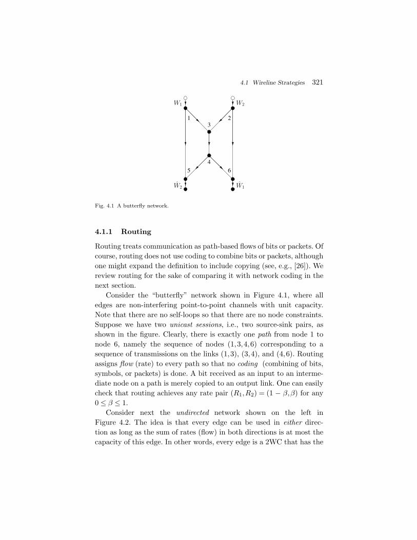
4.1 Wireline Strategies 321

Fig. 4.1 A butterfly network.

4.1.1 Routing

Routing treats communication as path-based flows of bits or packets. Ofcourse, routing does not use coding to combine bits or packets, althoughone might expand the definition to include copying (see, e.g., [26]). Wereview routing for the sake of comparing it with network coding in thenext section.

Consider the “butterfly” network shown in Figure 4.1, where alledges are non-interfering point-to-point channels with unit capacity.Note that there are no self-loops so that there are no node constraints.Suppose we have two unicast sessions, i.e., two source-sink pairs, asshown in the figure. Clearly, there is exactly one path from node 1 tonode 6, namely the sequence of nodes (1,3,4,6) corresponding to asequence of transmissions on the links (1,3), (3,4), and (4,6). Routingassigns flow (rate) to every path so that no coding (combining of bits,symbols, or packets) is done. A bit received as an input to an interme-diate node on a path is merely copied to an output link. One can easilycheck that routing achieves any rate pair (R1,R2) = (1 − β,β) for any0 ≤ β ≤ 1.

Consider next the undirected network shown on the left inFigure 4.2. The idea is that every edge can be used in either direc-tion as long as the sum of rates (flow) in both directions is at most thecapacity of this edge. In other words, every edge is a 2WC that has the

322 Cooperative Strategies and Rates

Fig. 4.2 An undirected butterfly network as a network of 2WCs.

capacity region shown in the middle of Figure 4.2. We thus redraw thisgraph as shown on the right in Figure 4.2. We further model every pairof edges between nodes u and v as Shannon’s push-to-talk 2WC [167,Sec. 1] defined by

(Yuv,Yvu) =

(Xuv,Zvu) if Xuv �= 0,Xvu = 0,

(Zuv,Xvu) if Xuv = 0,Xvu �= 0,

(Zuv,Zvu) if Xuv = Xvu = 0,

(4.1)

where (Zuv,Zvu) is uniform over Xuv × Xvu, and |Xuv| = 2Cuv + 1 forall edges (u,v). The channel (4.1) has the capacity region shown in themiddle of Figure 4.2.

Suppose that Cuv = 1 for all edges (u,v). Routing performs betterthan in Figure 4.1 because there are more paths available from eachsource to its sink. In fact, there are four paths from node 1 to node 6:path (1,3,4,6), path (1,3,2,6), path (1,5,4,6), and path (1,5,4,3,2,6).We can thus perform routing as shown in Figure 4.3 and achieve therate pair (R1,R2) = (1,1). This pair defines the capacity region of thisnetwork, since the cut-set bound of Section 3.7.1 gives R1 ≤ 1, R2 ≤ 1.In fact, the maximum flow for two unicast sessions on any undirectedgraph is given by the minimum cut [80]. Note also that one can separatechannel coding (PHY layer coding) and routing (network layer coding)to achieve the capacity for this special case. However, such separationof channel and network coding is not always optimal [152].


Fig. 4.3 An optimal routing for the undirected butterfly network.

4.1.2 Network Coding

We found that routing achieves a smaller rate region for the directednetwork of Figure 4.1 than for the undirected network in Figure 4.2.However, suppose that node 3 combines the packets arriving from nodes1 and 2 by XORing them bit-wise, shown as X1 ⊕ X2 in Figure 4.4.This combining of raw bits or packets is called network coding [4]. Morespecifically, it is called linear network coding if the combining opera-tions are done over a (finite) field [101, 116]. Node 5 collects X1 andX1 ⊕ X2 and computes X2. Similarly, node 6 collects X2 and X1 ⊕ X2

and computes X1. Thus, network coding achieves the capacity point

Fig. 4.4 Network coding for the directed butterfly network.


(R1,R2) = (1,1) even for the directed network of Figure 4.1, and thusoutperforms routing by a factor of two in rate. Furthermore, networkcoding gives an additional method for achieving capacity on the undi-rected network of Figure 4.2.

We remark that the rate gains of network coding over routing are thelargest for a multicast session, i.e., there is one source and many sinks.For example, the graph in Figure 4.5, which is a simple modificationof the graph in Figure 4.1, shows that R = 2 is feasible with networkcoding while only R = 1 is feasible with routing.

We further remark that the codes in Figures 4.4 and 4.5 were spe-cially chosen by using our knowledge of the network graph. In general,however, the individual nodes must operate without this information(see Table 1.1). An attractive coding method is then to use randomnetwork coding [4] or random linear network coding [73]. For the lat-ter approach, consider node u and let Ein(u) and Eout(u) be its sets ofincoming and outgoing edges, respectively. Suppose that every packethas L = nb data bits for some integers n and b. Coding at node u

proceeds as follows:

(a) for every pair (e,f) ∈ Ein(u) × Eout(u) choose a we,f ran-domly from the Galois field GF(2b);

Fig. 4.5 Network coding for a multicast network.


(b) collect one packet from each incoming edge e and strip off itsheaders to form the data string xL

e ;(c) parse xL

e into n pieces xbe(i), i = 1,2, . . . ,n, having b bits each;

(d) for every outgoing edge f compute∑e∈Ein(u)

we,f · xbe(i) (4.2)

for i = 1,2, . . . ,n, where the multiplications and additions areover the Galois field GF(2b);

(e) collect the n pieces corresponding to outgoing edge f intoxL

f ;(f) augment xL

f with a header that includes the we,f , e ∈ Ein(u),to inform the decoders of how the packets were combined;

(g) transmit the resulting packet on edge f .

Random linear network coding is known to work well if the size b of thepieces is sufficiently large and if the weights we,f are chosen indepen-dently and uniformly over GF(2b). For example, for practical reasonswe would like to use b = 1 so that the weights we,f are in GF(2) butthen one cannot guarantee that random network coding will work. Inthis case we must add redundancy, e.g., by using coding at the sourcesin the form of LT-codes or Raptor codes [128, 168]. The combinationof coding at the sources and network coding can provide good rate ver-sus reliability tradeoffs. Many other results on network coding can befound in a recent special issue of the IEEE Transactions on InformationTheory devoted in part to this topic [171].

4.1.3 Mode Coding

There are further rate gains possible in wireline networks beyondnetwork coding [105]. To show this, we consider the wireline net-work in Figure 3.3 with the node constraint (3.1) and Y3 = X2. Thegraph for this network is shown in Figure 4.6. Suppose for simplic-ity that the alphabets X1,X2,Y2,Y3 of the respective random variablesX1,X2,Y2,Y3 are all the set {0,1}. One might guess that the capacityis 1/2 bit/clock tick because the relay can either receive or transmit,but not both.


Fig. 4.6 A network graph with a relay device constraint.

Fig. 4.7 A code tree for the relay in Figure 4.6.

Consider, however, the code tree depicted in Figure 4.7 that islabeled with the symbols X2 that the relay transmits after havingdecoded an X1. The idea is that after decoding X1 = 0 the relay sendsX2 = 0, while after decoding X1 = 1 the relay uses the channel twiceto send the pair of symbols X2,1 = 1 and X2,2 = 0. Note that everycodeword in the code tree has exactly one 0, so that the source cantransmit exactly one new message bit for every relay codeword. Notefurther that the tree is labeled so that the code is prefix-free or instan-taneously decodable [34, Ch. 5]. This means that the sink can correctlyparse its received sequence to extract the message bits.

For example, suppose the message w has 8 bits 0,1,0,0,1,1,1,0. Thetransmit and receive sequences are then

i = 1, 2, 3,4, 5, 6, 7,8, 9,10, 11,12, 13Xn

1 = 0, 1, x,0, 0, 1, x,1, x,1, x,0, x

Y n2 = 0, 1, 0,0, 0, 1, 0,1, 0,1, 0,0, x

Xn2 = 0, 0, 1,0, 0, 0, 1,0, 1,0, 1,0, 0,

(4.3)

where x denotes a “do not care” symbol. Note that, for this particularmessage, we have transmitted 8 bits in n = 13 clock ticks which givesa rate R = 8/13 that is larger than 1/2.

We would like to determine the rate of the above code when thesource transmits b bits for large b. The codewords have variable lengths,so we define a random variable L2 to be the length of the codeword ofany of the message bits. If the source bits are coin-tossing, we compute

4.2 Wireless Strategies 327

E[L2] = 12(1) + 1

2(2) = 32 and

R =1

E[L2]= 2/3 bits/clock tick (4.4)

implying that we can substantially increase the rate beyond 1/2bit/clock tick. In fact, it turns out that better compression codes such asHuffman codes or arithmetic source codes (see [34, Ch. 5]) can achieveR = 0.773 bits/clock tick. Furthermore, this rate is the capacity of thenetwork, as one can check by computing the cut-set bound.

We call the above method mode coding because one is effectivelytransmitting information through the choice of the relay’s operatingmode (listen or talk).1 We will later consider this type of coding in moredetail for wireless relays. Note that the relative gains of mode coding aresmall when the alphabets X1,X2,Y2,Y3 are large. In fact, mode codingboosts the rate by at most 1 bit/packet over an edge time-sharingstrategy. But packets often have several thousands of bits. Furthermore,mode coding requires rapid on/off switching by the relay. On the otherhand, this coding might be useful for covert communication where, e.g.,a router time-jitters transmissions according to a signature pattern.

4.2 Wireless Strategies

The previous section shows how network coding combines raw bitsor packets at the network layer to improve rates. More generally, co-operative coding combines symbols at the physical and higher layers toproduce new symbols. We consider several types of cooperative codingstrategies, including

(1) amplify-and-forward (AF)(2) classic multi-hop(3) compress-and-forward (CF)(4) decode-and-forward (DF)(5) multipath decode-and-forward (MDF)(6) DF or MDF with network coding.

1 Mode coding seems related to sending “bits through queues” [7].


The above strategies can be used for both wireline and wireless net-works and they require progressively more coordination. For example,consider a RC. AF and classic multi-hop do not necessarily requirechanges at the source or destination nodes, e.g., for multi-hop the relaycan behave as if it is the destination or the source. CF does not nec-essarily require changes at the source but it does require some extraknowledge about the link capacities. DF requires changes at both thesource and destination, and MDF requires additional changes at higherlayers of the protocol stack. DF or MDF with network coding requireeven more changes at higher layers. Some of these issues are discussedin the sections below. However, we begin by specifying the models usedin this section.

4.2.1 Idealized Wireless Models

In this section, we will describe and compare wireless strategies byusing two idealizations:

• we consider full-duplex radios, i.e., devices that can transmitand listen at the same time in the same frequency band;

• if the channels are time-varying, we assume per-link channelstate information is available at the receiver but not at thetransmitter (CSIR, No CSIT, see Section 3.4).

We defer consideration of duplexing constraints to Section 4.3. Notethat full-duplex operation is often not possible due to large differencein transmit and receive power2 (see Section 3.3). However, full-duplexmodels have didactic utility in that their capacities can sometimes bewritten in closed-form. Furthermore, the information theory developedfor the full-duplex models applies directly to wireline problems and,perhaps surprisingly, to half-duplex models as well [103, 106].

The basic cooperative model is the relay channel shown inFigure 3.5 [33, 106]. In our derivations, we consider a general geometryshown in Figure 4.8(a) with nodes u and v at distance duv. For numeri-cal evaluations, we employ the linear geometry shown in Figure 4.8(b),

2 Some devices can operate in full-duplex mode with good echo cancellation.


Fig. 4.8 Relay channel geometries: (a) In general, nodes u and v are separated by distanceduv ; (b) In the linear case, the source-destination distance is d13 = 1, the source-relaydistance is d12 = |d| and the relay-destination distance is d23 = |1 − d|.

where the source and destination nodes are a distance d13 = 1 apart,and the relay is a distance d12 = |d| to the right of the source, and adistance d23 = |1 − d| to the left of the destination. A negative d meansthat the relay is to the left of the source. We remark that we are hereconsidering distances duv that are less than one, in seeming disregardof our claim in Section. 2.2.1 that we are interested in long-range com-munication where the model (2.3) is accurate. However, we are in effectnormalizing the source–destination distance to be unity, and includinglong-range attenuation in the power constraints. For example, when welater find in Section 4.2.6 that DF achieves capacity when the relayis near the source, the distance need not be less than one but rathershows where the relay must be relative to the source and destination.

We consider channels that exhibit one of three kinds of fading: (1)no fading; (2) fast uniform-phase fading; and (3) fast Rayleigh fading(see Section 3.2). That is, for every clock tick we have the complexchannels (see (3.3a) and (3.3b))

Y2 =H12

|d|α/2 X1 + Z2, (4.5a)

Y3 = H13 X1 +H23

|1 − d|α/2 X2 + Z3. (4.5b)

For no fading, the Huv are constants. For uniform-phase fading, theHuv are independent and uniform over {ej φ : φ ∈ [0,2π)}. For Rayleighfading, the Huv are independent and Gaussian with zero mean and unitvariance.


For CSIR, we assume that all nodes know the distances duv, butfor uniform-phase and Rayleigh fading Huv is known only to node v,i.e., only the relay knows H12, and only the destination knows H13

and H23. As in Section 3.4, we model this by augmenting Y2 and Y3

to become the vectors [Y2 H12] and [Y3 H13 H23], respectively. As wewill see, channels whose phase varies rapidly exhibit a special propertythat we exploit to derive capacity theorems. Furthermore, we shall latersee that making the relay half-duplex brings both complications andsimplifications to our theory and strategies.

4.2.2 Amplify-and-Forward

Amplify-and-forward has the relay transmit

X2,i = a2,iY2,i−1, (4.6)

where the a2,i, i = 1,2, . . . ,n, are chosen to satisfy the relay’s powerconstraint [59, 111, 161]. More generally, the relay might transmit somefunction of a small number of the past received symbols, e.g.,

X2,i = a2,i · [Y2,i−1 Y2,i−2 . . . Y2,i−D]T , (4.7)

where the a2,i, i = 1,2, . . . ,n, are row vectors chosen to satisfy the relay’spower constraint. Consider (4.6) where a2,i = a for all i so that we have(see (4.5b))

Y3,i =H13,i

dα/213

X1,i +H23,i

dα/223

X2,i + Z3,i, (4.8)

=H13,i

dα/213

X1,i + aH12,i−1H23,i

dα/212 d

α/223

X1,i−1 + aH23,i

dα/223

Z2,i−1 + Z3,i. (4.9)

To satisfy the power constraint, we require

|a|2 ≤ P2

N + P1E[|H12|2]/dα12

. (4.10)

Observe that, without fading, (4.9) is an AWGN channel with unit-memory intersymbol interference (ISI). In general, one should there-fore perform a waterfilling optimization of the spectrum of Xn

1 (cf.Section 2.2.5, Section 3.4, and [106, Sec. VII.B]). The result is shown in


−1 −0.75 −0.5 −0.25 0 0.25 0.5 0.75 10

1

2

3

4

5

6

upper boundDF

ρ for DF

CF

relay off

AF

d

Rat

e [b

it/us

e]

Fig. 4.9 Rates for a full-duplex relay, P1/N = P2/N = 10, Huv = 1 for all (u,v), and α = 2.

Figure 4.9 for the linear geometry of Figure 4.8(b) as the curve labeled“AF,” where P1/N = P2/N = 10, Huv = 1 for all (u,v) and α = 2. Therelay-off rate is simply log2(11). The curve labeled “upper bound” isthe cut-set bound (3.33). The other curves are based on the CF andDF strategies developed further below. Note that AF always performsas well as using no relay by choosing a = 0. Note also that increasing a

from 0 increases the destination’s ISI and noise power. The relay shouldthus not always transmit with maximum power.

The AF rates in Figure 4.9 are often significantly worse than therates achieved by other strategies. However, AF can sometimes performvery well [59]. For example, consider the RC with T relays3 shown inFigure 4.10. Suppose every relay u, u = 2,3, . . . ,T + 1, has

n∑i=1

E[|Xu,i|2

]/n ≤ P (4.11)

3 Note that T is here the number of relays rather than time.


Fig. 4.10 A multi-relay channel and geometry.

and E[|Zu|2] = N . If 0 < d < 1, Huv = 1 for all (u,v), and every relayuses AF as in (4.6) with au,i = a, then we have

Xu,i = aYu,i−1 (4.12)

and the T -relay version of (4.9) is

YT+2,i =Ta

|d(1 − d)|α/2 X1,i−1 + ZT+2,i +T+1∑u=2

a

|1 − d|α/2 Zu,i−1. (4.13)

Note that there is no channel from node 1 to node T + 2. Equation(4.13) thus defines an AWGN channel with SNR

γ =T 2|a|2P1

N [|d(1 − d)|α + T |a|2|d|α]. (4.14)

But the cut bound (3.24) in Section 3.7.1 with S = {1,2, . . . ,T + 1}gives

C ≤ log2

(1 +

T 2P

N

). (4.15)

We thus have

log2(T ) + log2

(P1

N· |a|21 + |a|2

)

< C ≤ 2log2(T ) + log2

(1T 2 +

P

N

)(4.16)

so that C grows as κ log2(T ) with T , where 1 ≤ κ ≤ 2. Furthermore,AF achieves this scaling law up to a constant factor.


The above scenario permits the total system power to grow linearlywith T . Instead, one might require P = Psum/T for some constant Psum.We choose (see (4.10))

|a|2 =Psum/T

N + P1/|d|α . (4.17)

Inserting (4.17) into (4.14) and (4.15), we find that

log2(T ) + log2

(Psum

N· P1

N + P1/|d|α + Psum

)

< C ≤ log2(T ) + log2

(1T

+Psum

N

). (4.18)

Now C grows as log2(T ) with T and AF achieves this scaling law up toa rate offset. We remark that both the scaling laws (4.16) and (4.18)require coherent combining of signals at the destination.

4.2.3 Classic Multi-Hop

Classic multi-hop has the source transmitting its message W to therelay in one-time slot, and then the relay forwarding W to the desti-nation in a second-time slot. This scheme can be used with both full-duplex and half-duplex relays. Suppose we assign the time fractions τ

to the first hop and τ = 1 − τ to the second hop. For constant H12 andH23, we achieve

R = min[τ log2

(1 +

P1|H12|2τdα

12N

), τ log2

(1 +

P2|H23|2τ dα

23N

)]. (4.19)

However, even after optimizing τ one always performs worse than usingno relay for any d in Figure 4.9. This happens because α = 2 is too smallto make multi-hopping useful. We will see later that multi-hop can workwell for half-duplex relays and larger α.

4.2.4 Compress-and-Forward

We continue to consider the no-fading case for simplicity. CF isa block-transmission strategy with the block structure shown inFigure 4.11 [33]. There are three codebooks: x1(·), x2(·), and a quanti-zation codebook y2(·). The source transmits x1(wb) indexed by a new


Source

Relay

Destination

Block 1 Block 4Block 3Block 2

Fig. 4.11 A CF strategy for a full-duplex relay.

message wb in every block b. The relay observes y2,bin block b and

chooses its next codeword as follows: y2,bis quantized to y2(sb−1,sb)

and the index sb chooses the codeword x2(sb). The destination firstdecodes sb using y3,b+1 and then decodes wb by using y2(sb−1,sb) andy3,b

. For the last block, the source transmits a default codeword x1(1).Consider, for example, the following relay encoding in block b. After

canceling the effect of x2(sb−1) on y2,b, the relay uses a vector quantizer

to map y2,bto y2(sb−1,sb) so that the average distortion (using some

per-letter distortion function) between these two vectors is at most D.Shannon’s rate-distortion theory [34, Ch. 13] tells us that the rate ofthe codebook y2(·) need to be at most

RQ(D) = I(Y2; Y2|X2). (4.20)

The relay can transmit sb reliably to the destination in block b + 1 viax2(sb) as long as

RQ(D) ≤ I(X2;Y3). (4.21)

The destination decodes sb and now knows x2(sb) and y2(sb−1,sb). Itfurther knows x2(sb−1) from its decoding in block b and can cancel theeffect of this vector on y2(sb−1,sb) and y3,b

. Finally, the destinationdecodes wb using y2(sb−1,sb) and y3,b

at the rate

R = I(X1; Y2Y3|X2). (4.22)

In fact, one can improve the rate specified by (4.20)–(4.22) by usinga more sophisticated vector quantizer and destination decoder [33].


The idea is that the relay transmits a hash h(sb−1) of the string sb−1

in block b, i.e., the relay sends x2(h(sb−1)) and finds a quantizationvector y2(h(sb−1),sb) in block b. The hashing is also known as binningand h(sb−1) is called a bin index. The result is that any rate R satisfying

R = I(X1; Y2Y3|X2) (4.23a)

subject to

I(Y2;Y2|X2Y3) ≤ I(X2;Y3) (4.23b)

is achievable where the joint probability distribution of the randomvariables factors as

P (x1,x2,y2,y3, y2) = P (x1)P (x2)P (y2,y3|x1,x2)P (y2|x2,y2). (4.24)

As done in (4.24), we will write PX(x) as P (x) if the argument of P (·)is a lower-case version of the random variable symbol. Note that theonly change from (4.20)–(4.22) is that the quantization codebook hasa lower rate than in (4.20), namely I(Y2;Y2|X2Y3). The factorization(4.24) reflects that the x1(wb) and x2 (h(sb−1)) codewords in block b arechosen independently, and that y2(h(sb−1),sb) is chosen as a functionof x2 (h(sb−1)) and y2,b

.A few remarks are in order. First, note that the rate (4.23) is the

rate of a point-to-point channel where the receiver has a vector output[Y2 Y3]. The CF strategy is thus closely related to multi-antenna recep-tion (see [57, 106]). In fact, if the relay-to-destination channel capacityis very large (say, if the relay is close to the destination) then the quan-tization code book can be very large and Y2 is “almost” Y2. The CFstrategy will then work well. Second, it is interesting that the maxi-mization of R in (4.23) turns out to be equivalent to the maximizationof (see [45])

R = min{

I(X1; Y2Y3|X2), I(X1X2;Y3) − I(Y2;Y2|X1X2)}

(4.25)

subject to (4.24). Third, one can time-share several modes of operationin (4.23) and (4.24), i.e., the source and relay use the respective distri-butions PX1|Q(·|q) and PX2|Q(·|q) for a fraction P (q) of the time, whereq represents one of a finite number of modes. Suppose that the source


and relay cycle through these modes several times. The relay can thencollect its quantization bits over all modes, and transmit them at theaverage rate I(X2;Y3|Q) to the destination. The result is that any ratesatisfying

R = I(X1; Y2Y3|X2Q) (4.26a)

subject to

I(Y2;Y2|X2Y3Q) ≤ I(X2;Y3|Q) (4.26b)

is achievable where the joint probability distribution of the randomvariables factors as

P (q)P (x1|q)P (x2|q)P (y2,y3|x1,x2)P (y2|x2,y2, q). (4.27)

The above rate sometimes improves the basic CF rate in (4.23) [45].In fact, one can similarly add a time-sharing random variable Q to allthe strategies in this chapter, but we will not consider this explicitly.Finally, note that the relay needs to know the statistics of Y3 to computeits compression and channel coding rates in (4.23b). The relay mightthus need to know {h13,i}n

i=1 and {h23,i}ni=1.

As a numerical example, suppose there is no fading. We chooseX1 and X2 to be the usual Gaussian distributions, and Y2 = Y2 + Z2

where Z2 = Z2R + jZ2I and Z2R and Z2I are independent, Gaussianrandom variables with variance N2/2 (this choice of Y2 is not necessarilyoptimal). The resulting information rates are

R = log2

(1 +

P1|H12|2dα

12(N + N2)+

P1|H13|2dα

13N

), (4.28a)

I(Y2;Y2|X2Y3) = log2

1 +

N

(P1|H12|2

dα12

+P1|H13|2

dα13

+ N

)

N2

(P1|H13|2

dα13

+ N

) ,

(4.28b)

I(X2;Y3) = log2

1 +

P2|H23|2dα

23

P1|H13|2dα

13+ N

. (4.28c)


The choice

N2 = N · P1|H12|2/dα12 + P1|H13|2/dα

13 + N

P2|H23|2/dα23

(4.29)

thus satisfies (4.23b) with equality (see also [57] and [79, Sec. 3.2]). Con-sider again the case P1/N = P2/N = 10, Huv = 1 for all (u,v), α = 2,and the linear geometry of Figure 4.8(b). The resulting CF rates areshown in Figure 4.9 as the curve labeled “CF.” Observe that CF per-forms well when the relay is close to the destination (d ≈ 1) and evenmeets the cut-set bound (3.33) when d = 1. Furthermore, CF signifi-cantly outperforms AF everywhere.

4.2.5 Decode-and-Forward

Decode-and-forward is a block-transmission strategy that has the blockstructure shown in Figure 4.12 [33, 106]. There are two code books:x1(·) and x2(·). The source uses block Markov encoding, i.e., the encod-ing has one block memory in that the source codeword in block b isx1(wb−1,wb). The idea is that the relay knows wb−1 and decodes wb

after having removed the effect of x2(wb−1). The resulting rate bound is

R ≤ I(X1;Y2|X2). (4.30)

The relay can now transmit x2(wb) in block b + 1. The destinationdecodes wb with a sliding-window decoder that uses y3,b

and y3,b+1(cf. [28, 191, 106]). If the codebooks of every block in Figure 4.12 werechosen independently, the resulting destination rate bound is

R ≤ I(X1;Y3|X2) + I(X2;Y3) = I(X1X2;Y3). (4.31)

The term I(X1;Y3|X2) in (4.31) comes from y3,b(note that the destina-

tion already knows wb−1 and thus x2(wb−1)) while the term I(X2;Y3)comes from y3,b+1 (x1(wb,wb+1) is treated as interference).

Relay

Source

Block 2 Block 4Block 3Block 1

Fig. 4.12 A DF strategy for a full-duplex relay.


Relay

Source

Block 3Block 2Block 1

Fig. 4.13 A DF strategy for a full-duplex relay on an AWGN relay channel.

Summarizing, DF achieves the rate

R = maxPX1X2 (·)

min{I(X1;Y2|X2), I(X1X2;Y3)} . (4.32)

The reader might wonder why one can optimize over all joint distribu-tions PX1X2(·). One can permit this by constructing the codebook x1(·)from x2(·) via superposition coding [32]. To explain this method, con-sider a full-duplex Gaussian relay channel with the DF block structureshown in Figure 4.13. The idea is that the code book x1(·) is constructedby adding (or superposing) codewords from a Gaussian codebook x′

1(·)to codewords from a Gaussian codebook x2(·) scaled by β. The code-words in x2(·) use power P2. The codewords in x′

1(·) use power P ′1,

where P ′1 ≤ P1, and the scaled codewords from x2(·) use power P1 − P ′

1,i.e., we have β =

√(P1 − P ′

1)/P2. Furthermore, the codeword x′1(wb) in

block b is independent of the codeword βx2(wb−1), so the source powerconstraint is satisfied.

The relay decodes wb at the rate log2(1 + P ′1|H12|2/(dα

12N)). Thedestination decodes wb by using y3,b

, y3,b+1, and its past estimate ofwb−1. The codeword x′

1(wb+1) is treated as interference. The resultingDF rate is

R =maxρ

min{

log2

(1 +

P1|H12|2(1 − |ρ|2)dα

12N

),

log2

(1 +

P1|H13|2dα

13N+

P2|H23|2dα

23N+

2√

P1P2�{ρH13H∗23}

dα/213 d

α/223 N

)},

(4.33)

where we recall that �{x} is the real part of x, and where ρ =E[X1X

∗2 ]/

√P1P2 is the correlation coefficient of the zero-mean X1 and

X2, which in this case is ρ =√

1 − P ′1/P1. Note that, by phase-rotating

the relay signal appropriately, the source and relay can coherently


combine their signals to give the destination an SNR boost. The pricepaid is a loss in the information rate from the source to the relay.

We make a few remarks. First, DF differs from classic multi-hop inseveral important ways:

(1) the source and relay transmit simultaneously(2) the source and relay signals can be made to coherently com-

bine at the destination if h13 and h23 are known to the trans-mitter or relay

(3) the destination decodes using several or all of its availableoutput blocks.

These differences remain for half-duplex relays. However, the seconddifference disappears for fast uniform-phase fading or fast Rayleighfading, as we shall see. Next, note that the last term in (4.32) is therate of a point-to-point channel where the transmitter has a vectorinput [X1 X2]. The DF strategy is thus closely related to multi-antennatransmission. In fact, if the source-to-relay channel capacity is large(say, if the relay is close to the source) then the limiting term in (4.32)is I(X1X2;Y3).

Consider again the case P1/N = P2/N = 10, Huv = 1 for all (u,v),α = 2, and the linear geometry of Figure 4.8(b). The resulting DF ratesare shown in Figure 4.9 as the curve labeled “DF.” The curve labeled“ρ for DF” shows the optimal correlation coefficient. Observe that DFperforms well when the relay is close to the source (d ≈ 0) and evenmeets the cut-set bound (3.33) when d = 0. Based on Figure 4.9, onewould choose DF if the relay is close to the source, and CF if the relayis close to the destination. This insight applies to other networks aswell. For example, suppose we have two relays. If both relays are closeto the source or the destination, then they should both use DF or CF,respectively. On the other hand, if one relay is close to the source andthe other is close to the destination, then the former relay should useDF while the latter should use CF.

4.2.6 CF and DF for Fast Uniform-Phase Fading

Consider the geometry of Figure 4.8(a) and where the Huv are fastfading. As noted in Section 4.2.1, we augment Y2 and Y3 to become


[Y2 H12] and [Y3 H13 H23], respectively. From (4.23), the CF rate isthus

R = I(X1; Y2Y3|X2H13H23) (4.34a)

subject to

I(Y2;Y2H12|X2Y3H13H23) ≤ I(X2;Y3|H13H23), (4.34b)

where

P (h,x1,x2,y2,y3, y2)

= P (h)P (x1)P (x2)P (y2,y3|x1,x2,h)P (y2|x2,y2,h12) (4.35)

and where h = [h12 h13 h23]. For uniform-phase fading, we have Huv =ejΦuv and choose Y2 = Y2e

−jΦ12 + Z2, where Z2, is the same as inSection 4.2.4. The result is that we recover the same rate as in (4.28a)–(4.29) (cf. [106]).

On the other hand, the DF rate is now

R = maxPX1X2 (·)

min{I(X1;Y2|X2H12), I(X1X2;Y3|H13H23)} . (4.36)

For the AWGN channel, this rate is

R = maxρ

min{

log2

(1 +

P1(1 − ρ2)dα

12N

),

E

[log2

(1 +

P1

dα13N

+P2

dα23N

+2ρej(Φ12−Φ13)√P1P2

dα/212 d

α/213 N

)]},

(4.37)

where the expectation is over the Φ12 and Φ13 that are independentand uniform over [0,2π). But Jensen’s inequality gives

E [log2(X)] ≤ log2 (E[X]) (4.38)

and we have E[ej(Φ12−Φ13)

]= 0. The best ρ in (4.37) is therefore

zero [79, 106]. This result is intuitive: without phase knowledge thesource and relay cannot coherently combine their signals at the des-tination. The DF block structure thus simplifies to that shown inFigure 4.14.


Relay

Source

Block 4Block 2 Block 3Block 1

Fig. 4.14 A DF strategy for a full-duplex relay and ρ = 0.

−1 −0.75 −0.5 −0.25 0 0.25 0.5 0.75 10

1

2

3

4

5

6

upper bound

DFCF

relay off

d

Rat

e [b

it/us

e]

Fig. 4.15 Rates for a full-duplex relay, uniform-phase fading, P1/N = P2/N = 10,and α = 2.

Figure 4.15 plots the CF, DF, and cut-set rates for the lin-ear geometry shown in Figure 4.8(b) and the uniform-phase fadingchannel with P1/N = P2/N = 10 and α = 2. Perhaps surprisingly, DFachieves capacity when the relay is in a region around the source [106].Figure 4.16 plots the two-dimensional positions of the relay whereDF achieves capacity when P1 = P2. Note that the region grows asα increases. The results in Figures 4.15 and 4.16 generalize to otherfast fading channels, e.g., Rayleigh fading channels, and it reinforcesthe insight from Section 4.2.5 that one should use DF when therelay is near the source. We remind the reader that the distances in


−1 −0.5 0 0.5 1

−1

−0.5

0

0.5

1

Source Destination

α=2

α=4 α=100

Fig. 4.16 Positions of the relay where DF achieves capacity with uniform-phase fading andP1 = P2.

Figures 4.15 and 4.16 should be interpreted as relative distances andnot as absolute ones.

4.2.7 Multipath Decode-and-Forward

Multipath decode-and-forward is a variation of DF where the sourcenode first performs rate-splitting, i.e., the message W with rate R issplit into W ′ and W ′′ having the respective rates R′ and R′′ such thatR′ + R′′ = R [33, 44, 106]. The same type of rate-splitting is done formultipath routing in Figure 4.3. In fact, MDF generalizes multipathrouting from wireline networks to wireless networks. Alternatively, onecould say that MDF combines multipath routing and DF.

The MDF block structure is shown in Figure 4.17. The idea is thatone replaces X1 in DF with an auxiliary random variable U , i.e., oneperforms DF with U playing the role of X1. The U represents codewordsu(w′

b−1,w′b) that transmit W ′, as shown in Figure 4.17. The “path” for

W ′ can thus be considered to be the entire RC [65]. On the otherhand, W ′′ is transmitted by the codewords x1(w′

b−1,w′b,w

′′b ) that are

superposed on u(w′b−1,w

′b) and x2(w′

b−1). The “path” for W ′′ can thusbe considered to be the direct link from the source to the relay.


Block 4Block 3Block 2Block 1

Source

Relay

Source

Fig. 4.17 An MDF strategy for a full-duplex relay.

Suppose the destination first decodes the messages w′b and then the

w′′b . Based on the above discussion, the rate of MDF is a sum of a DF

rate and a point-to-point rate:

R′ = min{I(U ;Y2|X2), I(UX2;Y3)} , (4.39a)

R′′ = I(X1;Y3|UX2), (4.39b)

where we can choose any P (u,x1,x2) and where we consider no fadingfor simplicity. The best MDF rate R = R′ + R′′ is therefore

R = maxPUX1X2 (·)

min{I(U ;Y2|X2) + I(X1;Y3|UX2), I(X1X2;Y3)} .

(4.40)

The MDF superposition method is shown for AWGN channels inFigure 4.18 that generalizes Figure 4.13. The codebook x1(·) is con-structed by adding codewords from the Gaussian codebooks u′(·),βx2(·), and u′′(·). The codewords in x2(·) use power P2. The code-words in u′(·) and u′′(·) have powers P ′

1 and P ′′1 , respectively, where

P ′1 + P ′′

1 ≤ P1. We must therefore choose β =√

(P1 − P ′1 − P ′′

1 )/P2.The decoding procedure is as follows. The relay decodes w′

b after receiv-ing y2,b

. The destination decodes w′b after receiving y3,b

and y3,b+1 byassuming that its past estimate of w′

b−1 is correct, and by treating

Source

Relay

Block 1 Block 2

Fig. 4.18 An MDF strategy for a full-duplex relay on an AWGN relay channel.


Node 1

Node 2 Node 3

Fig. 4.19 A mixed wireline/wireless relay channel and its graph.

u′(w′b+1) and u′′(w′′

b+1) as interference. Finally, the destination removesthe effect of u′(w′

b) from y3,band decodes w′′

b .Unfortunately, for full-duplex AWGN channels the MDF method

does not improve the DF method because the optimal choice ofPUX1X2(·) gives either DF or a point-to-point strategy. However, forother AWGN channels the MDF strategy performs better than DF.For example, we shall later see that MDF improves on DF for half-duplex channels. MDF even achieves capacity for an important class ofchannels discussed next.

Suppose we have the mixed network shown in Figure 4.19 where thesource-to-relay channel is a wireline channel. We model this by usingX1 = [X12 X13] and the channel

P (y2,y3|x1,x2) = P (y2|x12,x2)P (y3|x13,x2), (4.41)

where we permit X2 to contribute to Y2, i.e., the channel (4.41) includesport constraints such as (3.1). For the MDF rate (4.40), we chooseU = X12 and

P (x12,x13,x2) = P (x2)P (x12|x2)P (x13|x2). (4.42)

We compute

R = maxmin{I(X12;Y2|X2) + I(X13;Y3|X2), I(X13X2;Y3)} , (4.43)

where the maximization is over all distributions of the form (4.42).One can check that the cut-set bound (3.33) also gives (4.43) becausethe best input distributions factor as (4.42). The MDF rate (4.43) istherefore the capacity of the mixed relay channel [47].


We remark that this channel also models cases where nodes 1 and2 are wireless and the source-to-relay channel is “orthogonal” to thedestination channel. For example, this happens if the source-to-relaychannel uses a different frequency band than the destination channel.

4.2.8 Decode-and-Forward with Network Coding

Decode-and-forward can be combined with network coding in severalways, and we develop such strategies for two classes of wireless chan-nels in this and the next section. Consider first the network shown inFigure 4.20 and suppose the channels are defined by

Y1 =H31

dα/213

X3 + Z1, (4.44a)

Y2 =H32

dα/223

X3 + Z2, (4.44b)

Y3 =H13

dα/213

X1 +H23

dα/223

X2 + Z3, (4.44c)

where the Huv and Zu are the usual complex, Gaussian, random vari-ables. Note that this model orthogonalizes the MAC from nodes 1 and2 to node 3, and the BC from node 3 to nodes 1 and 2. For example,this could happen if nodes 1 and 2 are mobile stations and node 3 is abase station, and if one uses FDM for the uplink (MAC) and downlink(BC). AF, CF, and DF strategies for such channels have been analyzedin [100, 149, 150].

Suppose there is no fading with Huv = duv = 1 for all (u,v), thenoise variances are zero, and the alphabets of the Xu, u = 1,2,3, areall now binary. It is then easy to see that the best coding strategy is

Node 2Node 3Node 1

Fig. 4.20 A 3-node wireless network and its graph.


to use X3,i = X1,i−1 ⊕ X2,i−1 for all i. The resulting capacity is theset of (R1,R2) satisfying 0 ≤ R1 ≤ 1 and 0 ≤ R2 ≤ 1 (see, e.g., [190,Figure 1]).

Suppose next that there is fast uniform-phase fading with noise andcomplex alphabets as in (4.44a)–(4.44c). There are two natural codingapproaches. The first is similar to the binary case just described above:node 3 superposes codeword sequences for W1 and W2 over the modulo-lattice additive channels (MLACs) described in [48, 49] to satisfy itspower constraint.4 The second approach is to simply encode the pair(W1,W2) using a codebook with 2n(R1+R2) codewords x3(w1,w2) gen-erated by PX3(·). The latter method is directly related to broadcastingwhen receivers have side information [179] and should prove useful whenthere are non-uniform rates.5

For example, suppose we choose X1 and X2 as independent Gaus-sian random variables. The MAC bounds are

R1 ≤ log2

(1 +

P1

dα13N

), (4.45a)

R2 ≤ log2

(1 +

P2

dα23N

), (4.45b)

R1 + R2 ≤ log2

(1 +

P1

dα13N

+P2

dα23N

). (4.45c)

The BC rate bounds when using an MLAC (or a common codebookx3(·) as described above) to encode at node 3 are

R1 ≤ log2

(1 +

P3

dα23N

), (4.46a)

R2 ≤ log2

(1 +

P3

dα13N

). (4.46b)

In fact, the bounds (4.45a)–(4.46b) give the capacity region of ournetwork if the sum of (4.46a) and (4.46b) implies (4.45c). Onecan verify this by using the cut-set bound: the bound (3.24) with

4 We are grateful to S. Shamai for suggesting this approach.5 This approach was developed together with S. Shamai. The approach was also suggestedto us by E. Telatar, and independently appeared in [143] while this text was beingcompleted. The idea was further developed independently by L.-L. Xie.


S = {1},{2},{1,3},{2,3} gives (4.45a), (4.45b), (4.46a), and (4.46b),respectively.

4.2.9 Multipath Decode-and-Forward with Network Coding

Consider next the MAC-DR shown in Figure 4.21, where the X13 andX23 links are noise-free. Suppose X13 and X23 are binary while

Y4 =H14

dα/214

X14 +H24

dα/224

X24 +H34

dα/234

X3 + Z4, (4.47)

where H14, H24, H34, and Z4 are the usual complex, Gaussian, randomvariables. This model orthogonalizes the MAC from nodes 1 and 2 tonode 3, and the MAC from nodes 1, 2, and 3 to node 4.

One approach to coding is to apply existing MAC-DR strategiessuch as AF, CF, and DF [156, 157, 158, 159, 160]. Instead, for varietywe here wish to combine MDF strategies with network coding. Supposenodes 1 and 2 split their messages as Wu = [W ′

u W ′′u ] so that Ru =

R′u + R′′

u, u = 1,2. We further choose R′1 = R′

2 = 1 so that node 3 canXOR the W ′

1 and W ′2 bits it decodes and map them to a codeword in

the codebook x3(·).Node 1 associates its W ′

1 bits with an auxiliary random variable U1,and then superposes its W ′′

1 bits onto U1 via X1 as in Section 4.2.7.Node 2 uses similar steps. Node 4 first decodes W ′

1 and W ′2 jointly, strips

off their effect on Y4, and then decodes the W ′′1 and W ′′

2 . The MAC rate

Node 4

Node 1

Node 2

Fig. 4.21 A mixed wireline/wireless MAC-DR and its graph.


bounds for decoding W ′1 and W ′

2 at node 4 are

R′1 ≤ I(U1X3;Y4|U2H), (4.48a)

R′2 ≤ I(U2X3;Y4|U1H), (4.48b)

R′1 + R′

2 ≤ I(U1U2;Y4|X3H), (4.48c)

where [U1 X14], [U2 X24], and X3 are independent, and where H =[H14 H24 H34]. The bounds (4.48) are computed by considering the dif-ferent error events that can occur at node 4. The MAC rate bounds fordecoding W ′′

1 and W ′′2 at node 4 are

R′′1 ≤ I(X14;Y4|U1U2X3H), (4.49a)

R′′2 ≤ I(X24;Y4|U1U2X3H), (4.49b)

R′′1 + R′′

2 ≤ I(X14X24;Y4|U1U2X3H). (4.49c)

Combining the above rate bounds, we get an achievable region. How-ever, it is not clear that this region gives capacity points.

4.3 Half-Duplex Strategies and Mode Modulation

The information theory developed in the previous sections applies toboth full-duplex and half-duplex devices [106]. In this section, we con-sider the theory in more detail for half-duplex devices. For example, wedemonstrate that half-duplex nodes can transmit data by modulatingtheir “listen” to “talk” modes [103]. However, despite their fundamen-tal nature, one might not want to harness such mode modulation gainsfor reasons outlined below.

Consider a half-duplex RC with no fading. A DF strategy is depictedin Figure 4.22 where the relay listens for some fraction of the time andtalks for the other fraction of the time.6 Furthermore, all nodes knowahead of time when the relay listens and talks. We include the relay’soperating modes explicitly in the model as follows [103]. Let M2 be amode random variable that takes on the values M2 = L and M2 = T

if the relay listens and talks, respectively. One can check that the DF

6 Observe that the relay decodes all message blocks wb.

4.3 Half-Duplex Strategies and Mode Modulation 349

Relay

Source


Fig. 4.22 A DF strategy for a half-duplex relay channel.

strategy in Figure 4.22 achieves the rate

R = maxPX1X2M2 (·)

min{I(X1;Y2|X2M2), I(X1X2;Y3|M2)} . (4.50)

However, suppose we re-define the channel as P (y2,y3|x1,x2,m2),where the relay’s channel input is X ′

2 = [X2 M2]. We use X ′2 in place

of X2 in (4.32) and find that the DF rate is

R = maxPX1X2M2 (·)

min{I(X1;Y2|X2M2), I(X1X2M2;Y3)} . (4.51)

Expanding the second term on the right in (4.51), we have

I(X1X2M2;Y3) = I(M2;Y3) + I(X1X2;Y3|M2) (4.52)

and one can check that I(M2;Y3) > 0 in general. Thus, a strategy withpre-assigned slots such as in Figure 4.22 is generally suboptimal.

The reason for the rate gain I(M2;Y3) in (4.52) is that the relaysends information to the destination through its choice of operatingmode. In fact, this is how we achieve the wireline network capacityin Section 4.1.3. Mode modulation further improves all the strate-gies considered in Section 4.2, i.e., AF, classic multi-hop, CF, andDF or MDF with network coding. At the same time, there are somechallenges.

(1) I(M2;Y3) is limited to 1 bit/clock tick because M2 is binary.Thus, mode modulation cannot help much for channels withhigh capacity, e.g., wireline packet networks with large pack-ets (see Section 4.1.3) or AWGN channels with high SNR.

(2) The rate gain requires M2 to change rapidly. However, wire-line or wireless nodes cannot always switch from “listen” to“talk” modes rapidly.


(3) A remedy for the switching problem is to constrain the Mn2

sequence to change slowly, e.g., via run-length limited codes.However, this limits the rate gain even further.

The above reasons, as well as other considerations, usually lead oneto choose strategies as in Figure 4.22. We will do the same below (seealso [76, 98]). First, however, we show that mode modulation can giverate gains [103].

Consider the general relay geometry of Figure 4.8(a) and supposethere is no fading with Huv = 1 for all (u,v) and α = 4. Suppose fur-ther that we have per-symbol power-constraints P1 = P2 = 4, and thatthe relay must listen at least half the time to guarantee cooperation,i.e., PM2(L) ≥ 0.5. The DF rates (4.51), where the relay turns on andoff randomly, are shown in Figure 4.23 as the curve labeled “DF, ran-dom.” The DF rates (4.50), where the relay turns on and off at fixedtime-intervals, are shown as the curve labeled “DF, fixed.” The upperdash-dotted curve is the cut-set bound when using strategies as inFigure 4.23, and it is computed as (4.50) but with Y2 replaced by

−1 −0.75 −0.5 −0.25 0 0.25 0.5 0.75 10

0.5

1

1.5

2

2.5

3

3.5

4

4.5 cut−set bound for afixed slot strategy

DF, fixed

DF, random

Pr(M2=L) for DF

Pr(M2=L) for cut−set bound

relay off

d

Rat

e [b

it/us

e]

Fig. 4.23 Rates for half-duplex strategies with P1 = P2 = 4, Huv = 1 for all (u,v), andα = 4.

4.4 Multi-Antenna Relaying 351

[Y2 Y3]. Note that mode modulation outperforms any type of strat-egy with pre-assigned slots. The lower curves in Figure 4.23 show theoptimizing PM2(L) for both (4.50) and the cut-set bound.

4.4 Multi-Antenna Relaying

The information theory developed above applies to devices equippedwith multiple antennas in a similar fashion as in Section 2.2.5. We againmake the channel inputs and outputs vectors and write

Y 2 =H12

dα/212

X1 + Z2, (4.53a)

Y 3 =H13

dα/213

X1 +H23

dα/223

X2 + Z3, (4.53b)

where Xu, u = 1,2, and Y u and Zu, u = 2,3, are complex column vec-tors of length nu, and Huv is a complex nu × nv fading matrix. The Zu

have independent, Gaussian, variance N entries with the usual form.The matrix Huv is independent of Xu, u = 1,2, Zu, u = 2,3, and allother fading matrices. Rayleigh fading has Huv that have independent,Gaussian, zero-mean, unit variance entries with the usual form. Weconsider the general geometry of Figure 4.8(a).

The block power constraints are (see (2.26))

n∑i=1

E[‖Xu,i‖2]/n ≤ Pu, u = 1,2. (4.54)

However, we will here use the per-symbol constraints

E[‖Xu,i‖2] ≤ Pu, u = 1,2, i = 1,2, . . . ,n (4.55)

to avoid power control optimization.Consider first the point-to-point channel (4.53a) where node 1 sends

a message to node 2. The best X1 are zero-mean and Gaussian bythe maximum entropy theorem [34, p. 234]; recall that we write thecovariance matrix of X1 as QX1

. Since QX1is Hermitian, we can write

QX1= UΛU † where U is unitary, Λ is diagonal, and the eigenvalues of

QX1are on the diagonal of Λ [75, p. 171]. In particular, the trace of Λ


is the same as the trace of QX . The capacity is (see (3.10) and (2.28))

C = maxpX1 (·)

I(X1;Y 2 H12), (4.56)

= maxpX1 (·)

I(X1;Y 2 |H12), (4.57)

= maxQX1

∫hpH12(h) log

∣∣∣∣I +1

dα12N

(hU)Λ(hU)†∣∣∣∣dh, (4.58)

where, as usual, the maximizations are interpreted as constrainingpX1

(·) to satisfy the power constraints (4.55).Note that H12 U has the same distribution as H12 [174, Lemma 5].

We can therefore restrict attention to diagonal QX1, i.e., X1 that have

independent entries. Finally, recall that log |A| is strictly concave onthe convex set of positive definite Hermitian matrices A [75, p. 466].Furthermore, we can permute the entries of Λ without changing theintegral in (4.58). Averaging over all permutations and using the con-cavity of log |A|, we find that the best X1 has independent entries thateach have variance P1/n1. We thus have

C =∫

hpH12(h) log

∣∣∣∣I +(P1/n1)dα

12Nhh†∣∣∣∣ dh. (4.59)

We now return to our RC and model the half-duplex constraint asusual with

Y 2 =

H12

dα/212

X1 + Z2 if X2 = 0,

0 if X2 �= 0.

(4.60)

Alternatively, as in Section 4.3, we introduce a mode M2 that takes onthe values L and T . The MDF rate (4.40) is then

R = maxPU X1X2M2

min{I(U ;Y 2|X2M2) + I(X1;Y 3|U X2M2),

I(X1X2;Y 3|M2) + I(M2;Y 3) }, (4.61)

where U is a column vector of length n1, and where we have implicitlyaugmented the Y 2 and Y 3 with channel gains Huv as in Section 4.2.1and Section 4.2.6. However, we will ignore the expression I(M2;Y 3) byusing pre-assigned slots, as discussed in Section 4.3.

4.4 Multi-Antenna Relaying 353

Let V be a column vector of length n1 and let I be an appro-priately sized identity matrix. We choose U , V , and X2 to be inde-pendent, complex, Gaussian, zero-mean, and having covariance matri-ces (1 − β(M2))(P1/n1)I, β(M2)(P1/n1)I, and (P2/n2)I, respectively,where 0 ≤ β(M2) ≤ 1 (note that (4.55) prevents using power controlacross modes). We further choose X1 = U + V . The resulting expres-sions in (4.61) with the model defined by (4.53b) and (4.60) are

I(U ;Y 2|X2,M2 = L)

=∫

hp(h) log

∣∣∣∣I +P1

dα12n1N

hh†∣∣∣∣ ·∣∣∣∣I +

β(L)P1

dα12n1N

hh†∣∣∣∣−1

dh, (4.62a)

I(X1;Y 3|U X2,M2 = m2) =∫

hp(h) log

∣∣∣∣I +β(m2)P1

dα13n1N

hh†∣∣∣∣dh, (4.62b)

I(X1X2;Y 3|M2 = L) =∫

hp(h) log

∣∣∣∣1 +P1

dα13n1N

hh†∣∣∣∣dh, (4.62c)

I(X1X2;Y 3|M2 = T )

=∫

h,hp(h)p(h) log

∣∣∣∣I +P1

dα13n1N

hh† +P2

dα23n2N

hh†∣∣∣∣dhdh, (4.62d)

where the p(h) and p(h) are matrix fading distributions. Note that ford12 ≤ d13 it is best to choose β(L) = 0 and β(T ) = 1. Moreover, thisdistribution is basically the same as using the MDF strategy depictedin Figure 4.24 where X1 has the same distribution irrespective of M2.It therefore remains to optimize PM2(·). In fact, we shall avoid thisoptimization and consider only PM2(L) = PM2(T ) = 1/2.

So suppose we use the MDF strategy of Figure 4.24.7 We referto the RC as n1 × n2 × n3 based on the number of device antennas.

Relay

Source


Fig. 4.24 An MDF strategy for a half-duplex relay channel.

7 Observe that the relay decodes only the message blocks wb with odd indexes b.


−1 −0.75 −0.5 −0.25 0 0.25 0.5 0.75 10

0.2

0.4

0.6

0.8

1

1.2

1.4

1.6

1.8

2

MDF (relay talks 1/2 of time)

relay off

multihopping(optimum duplexing)

1x1x1 channel, 1/2−duplexRayleigh fading, α=4QPSK, γ

dB=3 dB

d

Rat

e [b

its/u

se]

Fig. 4.25 MDF rates for a 1 × 1 × 1 setup.

We consider two cases with QPSK modulation and Rayleigh fading[105, 104].

• A 1 × 1 × 1 setup with P1/N = P2/N = 2 (or γdB = 3 dB).The MDF rates are shown in Figure 4.25 as a functionof d. Also shown are the no-relay rate (R ≈ 1.13 bits/use)and the traditional multi-hopping rates with optimized listenand transmit times. Observe that MDF achieves substantialrate gains over both no-relay transmission and traditionalmulti-hopping. For instance, the points marked with ∗ inFigure 4.25 are (d,R) = (0.25,1.0) and (d,R) = (0.25,1.5).Note that the multi-hopping curve is well below the “relayoff” curve, and that the MDF curve is flat near d = 0.25.This happens because the source-to-relay link capacity isalmost saturated at the maximum QPSK rate of 2 bits/use.One should therefore use a larger modulation signal set, e.g.8-PSK, for the odd-numbered blocks in Figure 4.24.

• A 1 × 1 × 2 setup with P1/N = P2/N = 0.25 (or γdB =−6 dB). The MDF rates are shown in Figure 4.26. The

4.5 Code Design for Relaying 355

−1 −0.75 −0.5 −0.25 0 0.25 0.5 0.75 10

0.2

0.4

0.6

0.8

1

1.2MDF (relay talks 1/2 of time)

relay offmultihopping(optimum duplexing)

1x1x2 channel, 1/2−duplexRayleigh fading, α=4QPSK, γ

dB= 6 dB

d

Rat

e [b

its/u

se]

Fig. 4.26 MDF rates for a 1 × 1 × 2 setup.

figure also shows the no-relay rate (R ≈ 0.54 bits/use) andthe traditional multi-hopping rates with optimized listen andtransmit times. The points marked with ∗ in Figure 4.26 are(d,R) = (0.25,0.5) and (d,R) = (0.25,1).

4.5 Code Design for Relaying

We outline a code construction for half-duplex relays and for theRayleigh fading channels of Section 4.4. The design is based on a point-to-point multi-antenna strategy known as Diagonal Bell Labs LayeredSpace-Time (D-BLAST) [53]. Other code constructions for relay chan-nels are described in, e.g., [83, 200] (convolutional codes), [111] (space–time codes), [198] (turbo codes), [97, 104, 153, 50] (low-density parity-check (LDPC) codes).

We use two different codes: one for each of the two messages inthe first two blocks in Figure 4.24. The relay must decode w1 afterhaving received only the first block of outputs from the source. Wetherefore require Rc < 1/2 for the w1 encoder since half of the symbols


will be erased (we assume the even- and odd-numbered blocks in Fig-ure 4.24 have the same length; we further assume the source andrelay use the same signal/modulation set). We remark that MDF forhalf-duplex relaying does not suffer from error propagation, in con-trast to MDF for full-duplex relaying and D-BLAST for point-to-pointchannels.

Code design is usually done by using density evolution [154] orEXIT charts [175]. We use the latter approach and design irregularlow-density parity-check (LDPC) codes with the curve-fitting proce-dure described in [176]. The coded bits are mapped to QPSK symbolsvia the Gray mapping. The decoder uses the standard graph represen-tation of an LDPC code with variable nodes on the left and check nodeson the right. The left and right nodes are connected by edges whosenodes are chosen with a random permutation that avoids 2-cycles. Thedecoder iterates 60 times between the left and right nodes by using ana posteriori probability (APP) decoder.

Consider the 1 × 1 × 2 setup of Figure 4.26 and d = 0.25. ConsiderR = 1/2 without a relay. We design an LDPC code with rate Rc = 1/4and length nc = 8000 that has an (single-antenna, no fading, BPSK)AWGN decoding threshold of (Eb/N0)dB = −0.4 dB which is about 0.3dB from capacity. The resulting frame error rates (FER) are shown onthe right in Figure 4.27. Observe that the code operates within 1.5 dBof capacity at an FER of 10−3. The extra loss (as compared to 0.3 dBfor the single-antenna case) can be attributed to the short code lengthand the fading.

Consider next R = 1. We design an LDPC code with rate Rc = 3/8and length nc = 16,000 that has an (single-antenna, no fading, BPSK)AWGN decoding threshold of (Eb/N0)dB = 0.1 dB which is about 0.45dB from capacity. The encoding and decoding procedure is as follows(see Figure 4.24).

• In the odd-numbered blocks b = 1,3,5, . . ., the source trans-mits 4000 QPSK symbols (or 8000 of the 16,000 codewordbits) by using the rate Rc = 3/8 LDPC code.

• After every odd-numbered block b, the relay decodes theinformation bits of the Rc = 3/8 code from this block. Note

4.5 Code Design for Relaying 357

−7 −6.5 −6 −5.5 −5 −4.5 −4

10−3

10−2

10−1

100

1x2 no relayR=1/2 (R

c=1/4)

nc=8,000

2x2 distr. D−BLASTR=3/4 (R

c=3/8)

nc=16,000

1 detector activationrelay decodes early

R=1/2Capacity

R=3/4Capacity

d=0.25, α=4LDPC codesrandom edge perm.60 iterations

γdB

[dB]

Fra

me

Err

or R

ate

(FE

R)

Fig. 4.27 MDF frame error rates for the 1 × 1 × 2 scenario.

that the relay has received only half of this codeword’s sym-bols.

• In the even-numbered blocks b = 2,4,6, . . ., the source trans-mits using the rate Rc = 1/4 code described above.

• In the even-numbered blocks, the relay encodes the infor-mation bits decoded from the previous block by using theRc = 3/8 encoder and transmits the last 4000 QPSK sym-bols of this codeword (or the last 8000 of the 16,000 codewordbits).

• After every even-numbered block, the sink decodes the infor-mation bits of the rate Rc = 3/8 code. The sink performsonly one detector activation per codeword (we remark thatmultiple detector activations would improve the performancea little [176]).

• The sink cancels the interference caused by the symbols ofthe Rc = 3/8 code from the even-numbered blocks.

• After every even-numbered block, the sink decodes the infor-mation bits of the Rc = 1/4 code.


The overall rate is R = 2(3/8) + 2(1/4)(1/2) = 1 bit per use, wherethe leading factors 2 are due to the QPSK modulation. There are threedecoding steps to consider.

• The FER of the relay decoding step is not shown in Fig-ure 4.27 because it lies far to the left of the other two curves.

• The FER of the sink decoding the information bits fromthe Rc = 3/8 code is shown as the left curve in Figure 4.27(labeled “2 × 2 distr. D-BLAST”).

• The FER of the sink decoding the information bits from theRc = 1/4 code is the same as the case where there is no relay,and is the curve on the right in Figure 4.27.

We see that the dominating FER is in both cases (without andwith a relay) due to the direct link from the source to the sink. Thereliability of the two schemes is therefore the same. However, the MDFscheme doubles the rate.

5Cooperative Diversity

5.1 Introduction

The previous chapter examined cooperative strategies when no fadingor fast fading is present. The main performance metric was rate becauselong codes can average out the effects of noise and fading and can makethe error probability approach zero. In this chapter, we consider anotherextreme, namely, slow fading where the channel gains are random butare held constant for the duration of a codeword. For example, if achannel is in a deep fade then for high rates one cannot avoid makingerrors and we say there is an outage [54, 144]. We wish to characterizethe tradeoff between rate and outage probability. We again assume thatthe nodes have CSIR (see Sections 3.3, 4.1, and 4.2.1).

Outage probability can be reduced by means of diversity, i.e., trans-mitting signals carrying the same information over different paths intime, frequency, or space. For example, if ARQ feedback is available,then one can create diversity with Hybrid-ARQ (see Section 2.3). Oneof our aims is to create diversity through node cooperation.

Transmit cooperation has nodes using DF to exchange each other’smessages. By sharing resources, the nodes create two paths to transmit

359

360 Cooperative Diversity

their information (see Figure 3.1) and this is known as cooperationdiversity [162, 163] or cooperative diversity [112, 114]. Receive coop-eration has nodes forwarding information about their observations.For example, the nodes can use CF. A system with both transmitand receive cooperation resembles a multi-antenna or multiple-input,multiple-output (MIMO) system, and it is therefore sometimes calleda distributed MIMO system. It is known that multiple antennas canincrease capacity without sacrificing bandwidth or energy [53, 174]. Forinstance, if the path gains between the individual transmit and receiveantennas fade independently, high data rates are achieved by send-ing different data streams over the independent channels, an approachknown as spatial multiplexing [70].

Distributed MIMO systems can realize some of the usual MIMOgains. However, the absence of a high-capacity link (e.g., a cable)between the antennas limits the gains in several ways.

• The messages are known initially only to the source nodes.• Resources such as power, bandwidth and time (delay) must

be expended to enable cooperation.• Antenna power allocation cannot be performed as in conven-

tional MIMO systems.• Nodes may have half-duplex constraints.• Synchronizing signals sent from distributed antennas is more

difficult than in a conventional MIMO transmitter.

The effects of such limitations will become apparent once we analyzevarious cooperative protocols.

5.2 Performance Metrics

Consider a point-to-point channel as in Figure 2.2 and suppose thecoded modulation rate is R (see Section 2.2.3). Let γ be the averageSNR at the receiver and let I(γ) be the mutual information betweenthe channel inputs and outputs. Observe that I(γ) is a random variablethat depends on the fading coefficients. We will usually assume that thecodeword length n is sufficiently long and the codes sufficiently goodso that a decoding error is negligible if I(γ) > R. The event I(γ) < R

5.2 Performance Metrics 361

is called an outage and we write

Po(γ,R) = Pr[I(γ) < R]. (5.1)

We wish to characterize the achievable triples (γ,R,Po). For example,for a fixed R and Po we would like to determine the smallest possibleγ. However, such an analysis is often difficult so we instead study thelimiting behavior of (R,Po) when γ is large or small. As we shall see,one obtains important insight from these extreme cases.

5.2.1 High SNR Metrics

We consider the following performance metrics for large γ: diversitygain, multiplexing gain, and the diversity-multiplexing tradeoff.

5.2.1.1 Diversity Gain

For a given rate R, we define the diversity gain to be

d = limγ→∞

− logPo(γ,R)logγ

. (5.2)

The diversity gain thus determines the high-SNR slope of the outageprobability as a function of the average SNR when plotted on a log–logscale. For example, consider the slow Rayleigh fading channel with

Yi =H

dα/2 Xi + Zi, i = 1,2, . . . ,n, (5.3)

and the power constraint (2.4), i.e., the Zi and H are the usual complex,Gaussian random variables. Note that H is held fixed for all i and thatthe expected receive SNR is γ = (P/N)/dα. The mutual informationI(γ) with Gaussian inputs is

I(γ) = log2(1 + γ |H|2) bits/use. (5.4)

¿From (5.4), we thus have

Po(γ,R) = Pr[|H|2 <

2R − 1γ

]= 1 − exp

(− 2R − 1

γ

). (5.5)


To describe the outage behavior as a function of γ, we use the reciprocalof the normalized SNR (see [52, Sec. II.E])

g(γ,R) =22R − 1

γ. (5.6)

The outage probability (5.5) is thus

Po(γ,R) = 1 − e−g(γ,R/2) ∼γ g(γ,R/2), (5.7)

where the notation f1(x,y) ∼x f2(x,y) means that

limx→∞

f1(x,y)f2(x,y)

= 1. (5.8)

Observe from (5.6) and (5.7) that, up to a constant, the outage prob-ability decreases as 1/γ so the diversity gain (5.2) is d = 1.

We remark that for fixed coded modulations such as uncoded BPSK(see Section 2.2.2) we substitute the outage probability Po(γ,R) in(5.2) with the error probability Pe(γ). The BPSK error probability inRayleigh fading behaves as

Pe(γ) =14γ

(5.9)

and thus BPSK has d = 1 and R = 1.Finally, we remark that the diversity can alternatively be defined

for a family of codes {C(γ)} with rates R(γ) indexed by γ. In otherwords, the rate R in (5.2) changes with γ. This extension is usefulwhen studying multiplexing gains.

5.2.1.2 Diversity Gain for MISO Channels

One can generalize the above analysis for Rayleigh-fading MIMO chan-nels with n1 transmit and n2 receive antennas and show that the diver-sity gain is d = n1n2 [201]. For example, suppose there are n1 transmitantennas and one receive antenna, i.e., we have a multi-input, single-output or MISO channel. The model is (see Section 4.4)

Yi =H

dα/2 Xi + Zi, (5.10)


where H is a 1 × n1 vector with the usual independent Gaussian entries,and the Xi are n1 × 1 vectors satisfying the power constraint (4.54).Following steps outlined in Section 4.4, one can show that the best Xi

are independent, zero-mean, Gaussian, and with independent entries ofvariance βkP where

∑n1k=1 βk = 1. The resulting outage probability is

Po(γ,R) = Pr

[n1∑

k=1

βk|Hk|2 < g(γ,R/2)

]. (5.11)

The choice of βk, k = 1,2, . . . ,n1, that minimizes Po(γ,R) turns outto depend on γ and R [174, Section 5.1] and has not yet been char-acterized for n1 > 2. For n1 = 2, note that β1|H1|2 and β2|H2|2 areindependent random variables with distribution functions

Fu(x) = 1 − e−x/βu , x ≥ 0, u = 1,2. (5.12)

The distribution function of their sum is

F (x) =β1(1 − e−x/β1

) − β2(1 − e−x/β2

)β1 − β2

, x ≥ 0. (5.13)

Using (5.13), one can show that the optimal βk for n1 = 2 are: β1 = β2 =1/2 if R < log(1 + µoP ) where µo ≈ 1.2564, and β1 = 1 otherwise [94].

In general, however, we are mainly interested in large γ for whichone can show that βk = 1/n1 for all k is best. To see this, note that(5.11) is lower bounded by setting βk = 1 for all k, i.e., we have (see [148,Ch. 1])

Po(γ,R) ≥ 1 − e−g(γ,R/2)n1−1∑k=0

g(γ,R/2)k

k!(5.14)

∼γ g(γ,R/2)n1

n1!. (5.15)

Similarly, if we set βk = 1/n1 for all k then we can achieve

Po(γ,R) = 1 − e−n1g(γ,R/2)n1−1∑k=0

nk1

k!g(γ,R/2)k (5.16)

∼γ nn11

n1!g(γ,R/2)n1 . (5.17)


0 2 4 6 8 10 12 14 16 18 20

10−5

10−4

10−3

10−2

10−1

100

γDB

[dB]

Po(γ

, R)

n1=1

n1=2

n1=3

R = 2

R = 1BPSK

Fig. 5.1 Outage probabilities for MISO channels.

Thus, up to a constant, the outage probability decreases as γ−n1 so thatthe diversity gain (5.2) is d = n1. Figure 5.1 plots Po(γ,R) in (5.16) asa function of γdB = 10log10 γ for n1 = 1,2,3 and R = 1,2. Also shownis the BPSK error probability (5.9). Observe that BPSK outperformsthe random coding strategies with n1 = 1. However, one should keep inmind that an outage for BPSK means that one bit is in error, while anoutage for random codes means that an entire block of bits is in error.

5.2.1.3 Multiplexing Gain

Suppose we wish to study the limiting behavior of I(γ) without consid-ering the outage probability. To do this, we consider a family of codes{C(γ)} with rates R(γ) indexed by γ, as described above. The ratesR(γ) usually increase with γ. The multiplexing gain (or the number ofdegrees-of-freedom) is defined as

r = limγ→∞

R(γ)logγ

. (5.18)


For example, for a Rayleigh-fading MIMO channel with CSIR the max-imum multiplexing gain is r = min(n1,n2), which represents the rankof a randomly chosen gain matrix H. We will use R = r log2 γ.

5.2.1.4 Diversity-Multiplexing Tradeoff

To study the diversity and multiplexing gains together, we again con-sider a family of codes {C(γ)} with rates R(γ), and we compute thefamily’s diversity and multiplexing gains using (5.2) and (5.18). Itis interesting to characterize the boundary of the set of achievablerate pairs (d,r) over all cooperative protocols. For example, let d∗(r) bethe supremum of the set of possible d for a fixed r. Similarly, let r∗(d)be the supremum of the set of possible r for a fixed d. In analogy torate-distortion theory, we call d∗(·) the diversity-multiplexing functionand r∗(·) the multiplexing-diversity function.

For example, consider a MISO Rayleigh fading channel with CSIRfor which we know that Gaussian inputs with independent entries areoptimal. We use (5.17) and R = r log2 γ to compute

d∗(r) = limγ→∞

− log(nn11 /(n1!)) − n1 log

(γ−1 · (2r log2 γ − 1

))logγ

(5.19)

= n1(1 − r). (5.20)

The diversity-multiplexing function is therefore linear. This result gen-eralizes to MIMO channels with n1 transmit and n2 receive antennasas follows. For block lengths n with n ≥ n1 + n2 − 1, we find thatd∗(r) is a piecewise-linear function connecting the points (r,d∗(r)),r = 0,1,2, . . . ,min(n1,n2), where d∗(r) = (n1 − r)(n2 − r) (see [201]).

5.2.2 Low SNR Metrics

At low SNR, the system is limited by energy rather than multiplexinggain, and a meaningful metric is the rate R normalized by the SNR [182,183, 12]. For example, consider the channel (5.3) for which (5.5) gives

R(γ,Po) = log2 (1 − γ ln(1 − Po)) bits/use, (5.21)


where ln(x) is the natural logarithm of x. We define the low-SNR andSNR-normalized rate to be

R′(0,Po) = limγ→0

R(γ,Po) ln(2)γ

nats/use, (5.22)

where we have changed units to nats (1 bit = ln(2) nats). We compute

R′(0,Po) = − ln(1 − Po) nats/use, (5.23)

which gives R′(0,Po) ≈ Po nats when Po is small.Consider next the MISO Rayleigh fading channel (5.10) with n1

transmit antennas and βk = 1/n1 for all k. We define R′ = R ln(2)/γ

nats and use (5.16) to compute

limγ→0

g(γ,R/2) = R′ (5.24a)

limγ→0

Po = 1 − e−R′n1−1∑k=0

nk1

k!(R′)k. (5.24b)

Equation (5.24b) can be solved for R′ as in (5.23), but we will be mainlyinterested in small Po and hence small R′. Furthermore, small R′ iseffectively the same as small g(γ,R/2) or large γ in (5.14). Ignoringlow order terms, for small R′ we have (see [12])

R′(0,Po) ≈ (n1!)1/n1

n1P 1/n1

o nats. (5.25)

For example, for n1 = 2 and small Po we have R′(0,Po) ≈√P0/2. Thisis much larger than R′(0,Po) ≈ Po for n1 = 1 and small Po.

We remark that we can re-use our high-SNR analysis for low-SNR ifwe can make the “instantaneous” received SNR large by some means.This is, in fact, possible by using “bursty” transmission where a nodesignals for a short period of time, or in a small frequency band, withvery high power. Of course, such bursty transmission is not possible ifone has per-symbol power constraints such as (4.55) or a constraint onthe power per Hertz.

5.3 System Model 367

5.3 System Model

We study the performance of cooperative protocols for the networkshown in Figure 5.2. The network outputs are

Y1,i =

{H12

dα/212

X2,i + Z1,i if X1,i = 0,

0 if X1,i �= 0(5.26a)

Y2,i =

{H21

dα/221

X1,i + Z2,i if X2,i = 0,

0 if X2,i �= 0(5.26b)

Y3,i =H13

dα/213

X1,i +H23

dα/223

X2,i + Z3,i (5.26c)

for i = 1,2, . . . ,n. The transmitting nodes have half-duplex constraints.The noise variables Zu,i, u = 1,2,3, i = 1,2, . . . ,n, and channel gainsHuv are the usual complex, Gaussian random variables (see Section 3.2and (3.3a) and (3.3b)). Note that the Huv change on a slow timescaleas compared to the Xu,i and Zu,i. The transmitters have the averagepower constraints (3.5) and we set P1 = P2 = P for simplicity. We willusually view the network of Figure 5.2 as either a RC with node 1 asthe source, or a RC with node 2 as the source. Of course, this meansthat all the relaying strategies developed in Chapter 4 will apply here.

We add some remarks about channel and network knowledge. TheDF protocols usually require CSIR only. The AF protocols addition-ally require the destination to know the source-to-relay channel gain

Node 2

Node 1

Node 3

Fig. 5.2 A three-node wireless network. Nodes 1 and 2 have messages destined for node 3.


to perform maximal ratio combining [148, p. 721]. The CF protocolsrequire both the relay and destination to know all channel gains, i.e., therelay must have CSI available before transmitting (CSIT). The CSITusually has low rate as compared to the data, and requires feedbackfrom the destination once this node determines the channel gains onits incoming links. Keeping this in mind, we will see that CF achievesthe best possible diversity-multiplexing tradeoff in both the high andlow SNR regimes. Low rate feedback in the form of an ARQ bit fromthe destination to the relay can also improve performance, as shown inSection 5.4.2.5.

Finally, we remark that from now on we work with

γ = P/N (5.27)

rather than the received SNRs γuv = (P/N)/dαuv. For convenience, we

abuse notation and generically write mutual information expressionsparameterized by γ as I(γ) and then define Po(γ,R) = Pr[I(γ) < R].

5.4 Cooperative Strategies for High SNR

We consider two classes of strategies by distinguishing whether thesources transmit at the same time and in the same frequency bandor not.1 Strategies for which the sources do not interfere are calledorthogonal strategies. Such schemes are meant to achieve high diver-sity gains rather than high rates [112], although orthogonal strategiesare good enough for low SNR (see Section 5.5). Non-orthogonal strate-gies use bandwidth more efficiently and thus generally exhibit betterdiversity-multiplexing tradeoffs [14, 139, 193]. For example, a coopera-tive scheme known as dynamic DF achieves the diversity-multiplexingfunction for low values of multiplexing gains [14]. For larger values,multipath DF (see Section 4.2.7) outperforms dynamic DF [11]. Inter-estingly, CF achieves the diversity multiplexing function for all multi-plexing gains and for any number of antennas at the nodes [196], butrecall that it needs extra CSI at the relay and destination.

1 The following material is based mostly on [112].

5.4 Cooperative Strategies for High SNR 369

n / 2 n / 2

n / 4n / 4 n / 4 n / 4

Fig. 5.3 Channel allocation for: (a) orthogonal direct transmission, (b) orthogonal relaying.

5.4.1 Direct Transmission

Consider the network in Figure 5.2 and the TDM strategy inFigure 5.3(a). This strategy is cooperative in the sense that the usersdo not interfere with each other, and the destination’s signals are

Y3,i =

H13

dα/213

X1,i + Z3,i, i = 1,2, . . . ,n/2

H23

dα/223

X2,i + Z3,i, i = n/2 + 1, . . . ,n.(5.28)

The outage probability for nodes u = 1,2 is (see (5.7))

Po(γ,R) = 1 − e−g(γ,R) dαu3/2 (5.29)

∼γ g(γ,R) dαu3/2, (5.30)

where we remark that both nodes can send with twice their averagepower in their time slots. Observe that, up to a constant, the outageprobabilities decrease as 1/γ (or 1/γ).

5.4.2 Orthogonal Relaying Strategies

Consider next the cooperative strategy in Figure 5.3(b). During timesi = 1,2, . . . ,n/4, node 1 transmits and nodes 2 and 3 receive

Y2,i =H12

dα/212

X1,i + Z2,i, i = 1,2, . . . ,n/4 (5.31a)

Y3,i =H13

dα/213

X1,i + Z3,i, i = 1,2, . . . ,n/4. (5.31b)


During times i = n/4 + 1, . . . ,n/2, node 2 transmits X2,i as a functionof Y

n/42 . Node 2 thus acts as a relay and the destination receives

Y3,i =H23

dα/223

X2,i + Z3,i, i = n/4 + 1, . . . ,n/2. (5.31c)

During time i = n/2 + 1,n/2 + 2, . . . ,n, the roles of nodes 1 and 2 arereversed and the same procedure is repeated. We next consider severalways in which the relays process their received symbols.

5.4.2.1 Amplify-and-Forward

Suppose node 2 uses AF and forwards

X2,i = aY2,i−n/4, i = n/4 + 1, . . . ,n/2, (5.32)

while choosing a to satisfy its power constraint, i.e., we set (see (4.10))

|a|2 =2γ

1 + 2|H12|2γ/dα12

, (5.33)

where we recall that γ = P/N and the relay sends at twice its averagepower in its time slot. To decode, the destination combines thereceived signals (5.31b) and (5.31c) using maximum-ratio combiningwhich requires knowledge of |H12|2/dα

12. With Gaussian codebooks, oneachieves

I(γ) =14

log2

(1 + 2γ

( |H13|2dα

13+

2γ|H12|2|H23|2/(dα12d

α23)

1 + 2γ(|H12|2/dα12 + |H23|2/dα

23)

)),

(5.34)where the factor 1/4 is because nodes 1 and 2 transmit only 1/4 of thetime for each message. The outage event I(γ) < R is the same as

|H13|2dα

13+

2γ|H12|2|H23|2/(dα12d

α23)

1 + 2γ(|H12|2/dα12 + |H23|2/dα

23)< g(γ,2R)/2. (5.35)

For high SNR, one can show that the outage probability is given by(see [112])

Po(γ,R) ∼γ g(γ,2R)2 dα13(d

α12 + dα

23)/8. (5.36)

The diversity gain is thus d = 2, and this is the best possible. To seethis, note that the outage probability must be larger than when the


relay knows the source message ahead of time, effectively creating aMISO channel with n1 = 2 transmit antennas. We thus have d ≤ 2 byapplying (5.15).

5.4.2.2 Compress-and-Forward

Suppose the relay uses CF with the relay mode M2 acting as a time-sharing random variable (see Sections 4.2.4 and 4.3). The rates are

R =14I(X1; Y2Y3 |H,M2 = L) (5.37a)

subject to

I(Y2;Y2|Y3 H,M2 = L) ≤ I(X2;Y3|H,X1 = 0,M2 = T ) (5.37b)

p(h,m2,x1,x2,y2,y3, y2) = p(h)p(m2)p(x1|m2)p(x2|h,m2)

p(y2,y3|x1,x2,h)p(y2|x2,y2,h,m2), (5.37c)

where H = [H12 H13 H23]. We choose Y2 = Y2 + Z2 when M2 = L

as in Section 4.2.4. The rate (5.37a) is a quarter of (4.28a) andI(Y2;Y2|Y3 H,M2 = L) is the same as (4.28b) with P1 = P2 = 2P . Wealso have

I(X2;Y3|H,X1 = 0,M2 = T ) = log2

(1 + 2γ

|H23|2dα

23

). (5.38)

We thus choose

N2 = N · 1 + 2γ(|H12|2/dα

12 + |H13|2/dα13)

(1 + 2γ |H13|2/dα13) 2γ |H23|2/dα

23(5.39)

to satisfy (5.37b) with equality. The resulting outage event is

|H13|2dα

13+

2γ |H12|2dα12

|H23|2dα23

1 + 2γ

{(1 + 2γ |H13|2

dα13

)−1 |H12|2dα12

+ |H23|2dα23

} <g(γ,2R)

2,

(5.40)which clearly implies the AF outage event (5.35). The diversity gain isthus again d = 2. Note, however, that the relay and destination needfull CSIT and CSIR, respectively.


5.4.2.3 Decode-and-Forward

We first consider a suboptimal DF strategy that uses a repetition codeat the relay, i.e., the relay decodes the source message, re-encodes usingthe same codebook, and transmits. For Gaussian codebooks, we com-pute (see (4.32))

I(γ) = min{

14

log2

(1 + 2γ

|H12|2dα

12

),

14

log2

(1 + 2γ

( |H13|2dα

13+

|H23|2dα

23

))}. (5.41)

The outage event IDF < R is thus the same as

min{ |H12|2

dα12

,|H13|2dα

13+

|H23|2dα

23

}< g(γ,2R)/2 (5.42)

and we have

Po(γ,R) ∼γ g(γ,2R) dα12/2. (5.43)

Observe that d = 1 and this DF strategy offers no diversity gain overnon-cooperative communication. In fact, we obtain the same type ofresult if we use the usual DF strategy, where the only change is thatthe second logarithm in (5.41) increases to

14

log2

(1 + 2γ

|H13|2dα

13

)+

14

log2

(1 + 2γ

|H23|2dα

23

)(5.44)

and a similar change is made in (5.42). The deficiency in both DFstrategies is that we force the relay to decode even if |H12|2 is small.

5.4.2.4 Selection Decode-and-Forward

To overcome the drawback of DF, we compare the measured chan-nel gain |H12|2/dα

12 at the relay with a pre-specified threshold. If|H12|2/dα

12 is above the threshold, then the source remains silent and therelay forwards the information (either via a repetition code or anothercode). Otherwise, the source repeats its transmission. Observe that thismethod requires the relay to send one feedback bit to the source afterevery other transmission block. We call this a selection DF strategy.


We remark that the source must limit its transmit power to less than2P in its time slots. However, if Po is small, as we shall assume, thenthe source rarely needs to transmit twice. Hence, we have the sourcetransmit with power 2P in its first time slot and with a small amountof extra power in the second time slot if need arises (alternatively, thesource never transmits in the second time slot).

Suppose the relay uses a repetition code. We compute

I(γ) =

14 log2

(1 + 2γ |H13|2

dα13

)if |H12|2

dα12

< g(γ,2R)/2,

14 log2

(1 + 2γ

( |H13|2dα13

+ |H23|2dα23

))if |H12|2

dα12

> g(γ,2R)/2.

(5.45)Observe that we chose the threshold so that the direct transmissionis repeated if there is an outage on the source-relay link. The overalloutage event is A ∪ B where

A ={

min{ |H12|2

dα12

,|H13|2dα

13

}< g(γ,2R)/2

}(5.46a)

B ={ |H13|2

dα13

+|H23|2dα

23< g(γ,2R)/2

}(5.46b)

and so we have

Po(γ,R) ∼γ g(γ,2R)2 dα13(2dα

12 + dα23)/8, (5.47)

which is identical to (5.36) except for the factor of 2 in front of dα12.

This factor arises because A has twice the probability of B for largeγ. Other DF strategies achieve similar performance [82, 84, 86, 125,126, 172, 173]. The results are summarized in Table 5.1 where we setdα

uv = 2 for all (u,v).

Table 5.1 Diversity gains of orthogonal cooperative strategies for dαuv = 2.

Cooperativestrategy

High SNRperformance

Comment Extra CSI

Direct trans. g(γ,R) No diversityDF g(γ,2R) No diversitySelection DF 3

2 g(γ,2R)2 Full diversity 1 bit feedbackAF g(γ,2R)2 Full diversity |H12|2/dα

12 to dest.CF g(γ,2R)2 Full diversity Relay CSIT,

|H12|2/dα12 to dest.


5.4.2.5 Incremental Relaying

An inspection of the selection DF strategy reveals that if |H13|2/dα13 is

above the threshold g(γ,2R)/2 then the relay need not decode the mes-sage. Instead, the source can improve its rate by sending fresh informa-tion in the next time slot (as in hybrid ARQ or incremental redundancyARQ). The resulting strategy operates at source power P and rate R/2when the destination reception is successful, and at source power P/2and rate R/4 otherwise. Let

Po,13(γ,R) = Pr[ |H13|2

dα13

< β1 g(γ,R)], (5.48)

where β1 = P/P1 and P1 is the power the source can use when trans-mitting, i.e., P1 satisfies

P = P1(1 − Po,13(γ,R)) + (P1/2)Po,13(γ,R). (5.49)

We wish to compute the expected rate

R =R

2(1 − Po,13(γ,R)) +

R

4Po,13(γ,R) (5.50)

=R

2e−β1g(γ,R/2) +

R

4

(1 − e−β1g(γ,R/2)

). (5.51)

A complication arises in that several values of R can give the sameR; we choose the smallest R that satisfies (5.50). One can show thatincremental DF achieves full diversity, and that somewhat better resultsare possible with incremental AF (see [112, Sec. IV.E]). We remark,however, that this analysis implicitly requires using many fading blocksrather than just one.

5.4.3 Non-orthogonal Cooperative Strategies

The TDM constraint limits the rate more than necessary. We nextconsider non-orthogonal strategies that give good diversity multiplex-ing tradeoffs; for AF see also [139, 14, 193], for DF see [14], and for CFsee [196].



Consider two consecutive symbol transmissions from the source. Duringthe first symbol transmission, the relay listens. In the next symbolperiod, the source transmits a new symbol and the relay uses AF.Thus, the relay effectively creates an intersymbol-interference channel(see Section 4.2.2). One can show that this AF strategy achieves thediversity-multiplexing pairs (d,r) satisfying (see [14])

d = (1 − r) + (1 − 2r)+, (5.52)

where (x)+ = x if x > 0 and (x)+ = 0 if x ≤ 0. This strategy achieves abetter diversity-multiplexing tradeoff than orthogonal AF. However, forr > 1/2 this strategy is only as good as non-cooperative transmissionbecause of the half-duplex constraint. This drawback is removed withthe next strategy.

5.4.3.2 Dynamic Decode-and-Forward

Suppose the relay listens until it collects sufficient energy to decode thesource message. It then re-encodes the message with its own codebookand transmits for the remaining time that the source transmits [93,134, 136]. One can show that this dynamic DF scheme achieves thediversity-multiplexing pairs (d,r) satisfying

d =

{2(1 − r) if 0 ≤ r ≤ 0.5,

(1 − r)/r if 0.5 ≤ r ≤ 1.(5.53)

Observe that the diversity gain is the same as for a n1 = 2 MISO sys-tem for 0 ≤ r ≤ 1/2. For r > 1/2, unfortunately, the relay cannot helpenough of the time to achieve the MISO upper bound.

5.4.3.3 Compress-and-Forward

Suppose the relay listens half the time and uses CF. One can showthat CF achieves the MISO upper bound for 0 ≤ r ≤ 1, so we haved∗(r) = 2(1 − r) [196, Sec. VI]. In fact, CF achieves the MISO upperbound for any number of antennas at the source, relay, and destinationnodes. Note again, however, that the relay and destination need full


Table 5.2 Diversity-multiplexing tradeoff of non-orthogonal cooperative strategies.

Cooperative strategy d∗(r) Extra CSINo cooperation 1 − rOrthogonal AF 2 − 4r |H12|2/dα

12 to dest.Orthogonal DF 2 − 4rNon-orthogonal AF (1 − r) + (1 − 2r)+ |H12|2/dα

12 to dest.

Dynamic DF

{2(1 − r) 0 ≤ r ≤ 0.5(1 − r)/r 0.5 ≤ r ≤ 1

Relay wait time

CF 2(1 − r) Relay CSIT,|H12|2/dα

12 to dest.MISO bound 2(1 − r) Message to relay.

0 0.1 0.2 0.3 0.4 0.5 0.6 0.7 0.8 0.9 10

0.2

0.4

0.6

0.8

1

1.2

1.4

1.6

1.8

2

multiplexing gain r

dive

rsity

gai

n d

dynamic DF

CF andMISO upper bound

nonorthogonalAF

orthogonal AF andorthogonal DF

no cooperation

Fig. 5.4 Diversity-multiplexing tradeoff of non-orthogonal cooperative strategies.

CSIT and CSIR, respectively. The results are summarized in Table 5.2and the diversity-multiplexing pairs are plotted in Figure 5.4.

5.5 Relaying Strategies for Low SNR

We next turn our attention to low SNR. However, for simplicity wefocus on the RC rather than the network of Figure 5.2. We again con-sider TDM and orthogonal cooperative strategies: the source transmits

5.5 Relaying Strategies for Low SNR 377

half the time, and the relay listens and talks half the time.2 However,we will let the source transmit for a fraction β of the time with powerP/β during its transmit slot (see [12, 46]).

5.5.1 Cut-Set Bound

Recall that we used the MISO diversity gain to upper bound the coop-erative diversity gain. Unfortunately, for low SNR the MISO rates aretoo good and we need a better method. Consider the cut-set bound(3.33) for full-duplex relay channels. We compute

R ≤maxρ

min{

log2

(1 + γ

( |H12|2dα

12+

|H13|2dα

13

)(1 − |ρ|2)) ,

log2

(1 + γ

[H13

dα/213

H23

dα/223

][1 ρ

ρ∗ 1

][H∗

13/dα/213

H∗23/d

α/223

])}, (5.54)

where ρ = E[X1X∗2 ]/P . We remark that we could take ρ to be real

because Rayleigh fading has uniform phase.For example, suppose we choose ρ = 0. The outage probability

Po(γ,R/2) is then lower-bounded by the event

1dα

13|H13|2 + min

{1

dα12

|H12|2, 1dα

23|H23|2

}< g(γ,R/2). (5.55)

The distribution function of the minimum in (5.55) is

F (x) = 1 − e−x(dα12+dα

23). (5.56)

Combining (5.56) with (5.13), we obtain the distribution function ofthe left-hand side of (5.55) and can bound

Po(γ,R/2) ≥ (dα12 + dα

23)e−g(γ,R/2)dα13 − dα

13 e−g(γ,R/2)(dα12+dα

23)

(dα12 + dα

23) − dα13

(5.57)

∼γ g(γ,R/2)2 dα13(d

α12 + dα

23)/2. (5.58)

Note that (5.58) is a high SNR result, but it requires only that g(γ,R/2)is small. We will soon use (5.58) for low SNR. However, we must firstcheck that ρ = 0 gives the weakest cut-set bound.

2 The following material is based mostly on [12].


Consider again (5.54) and write the second logarithm as

log2

1 + γ [H13 H23]

1

dα13

ρ

dα/213 d

α/223

ρ∗

dα/213 d

α/223

1dα23

[ H∗

13H∗

23

] . (5.59)

The 2 × 2 matrix in (5.59) is Hermitian and decomposes as UΛU †

where U is unitary and Λ is diagonal with entries λ1 and λ2 that satisfy

λ1 + λ2 = 1/dα13 + 1/dα

23, λ1λ2 =1 − |ρ|2dα

13dα23

. (5.60)

But recall from Section 4.4 that [H12 H13]U has the same statistics as[H12 H13], so we can write (5.59) as

log2

(1 + γ

(λ1 |H13|2 + λ2 |H23|2

)), (5.61)

where H13 and H23 have the same distribution as H13 and H23 and areindependent of H12. The outage probability Po(γ,R/2) is thus largerthan the probability of the event A ∪ B where (see (5.54))

A ={

1 − |ρ|2dα

12|H12|2 +

1 − |ρ|2dα

13|H13|2 < g(γ,R/2)

}, (5.62a)

B ={

λ1 |H13|2 + λ2 |H23|2 < g(γ,R/2)}

. (5.62b)

We have Pr[A ∪ B] = Pr[A] + Pr[B] − Pr[A ∩ B]. Consider first A forwhich it is clearly best to choose |ρ| as small as possible. In fact, using(5.13) we have

Pr[A] ∼γ g(γ,R/2)2dα

12 dα13

2(1 − |ρ|2) (5.63)

so to improve on (5.58) for ρ = 0 we must have |ρ|2 < 1 − dα12/(dα

12 +dα

23) (note that Pr[B] − Pr[A ∩ B] ≥ 0). Consider next B for which weuse (5.13) and (5.60) to compute

Pr[B] ∼γ g(γ,R/2)2dα

13 dα23

2(1 − |ρ|2) . (5.64)

Furthermore, one can check that the event A ∩ B implies the event

max{

1 − |ρ|2dα

12|H12|2,λ1 |H13|2,λ2 |H23|2

}< g(γ,R/2), (5.65)

5.5 Relaying Strategies for Low SNR 379

where the three random variables are independent. We thus have

Pr[A ∩ B] ≤(1 − e−g(γ,R/2)dα

12/(1−|ρ|2))

×(1 − e−g(γ,R/2)/λ1

)(1 − e−g(γ,R/2)/λ2

)(5.66a)

∼γ g(γ,R/2)3dα

12 dα13 dα

23(1 − |ρ|2)2 . (5.66b)

Summarizing, the combination of (5.63), (5.64), and (5.66b) shows thatρ = 0 gives the weakest high-SNR cut-set bound.

Finally, recall that we are interested in low SNR and not high SNR.We set R′ = R ln(2)/γ in (5.57) and use limγ→0 g(γ,R/2) = R′ to com-pute

limγ→0

Po ≥ (dα12 + dα

23)e−R′dα13 − dα

13 e−R′(dα12+dα

23)

(dα12 + dα

23) − dα13

. (5.67)

For sufficiently small R′ or Po, we thus have (see (5.58))

R′(0,Po) ≤√

2Po

dα13(d

α12 + dα

23). (5.68)

We shall see that AF and CF can approach the rate on the right-handside of (5.68).


Consider the basic orthogonal AF strategy of Section 5.4.2.1. If γ issmall, then the outage event (5.35) becomes

|H13|2dα

13< g(γ,R)/2 (5.69)

and hence we have

R′(0,Po) ≈ Po/dα13. (5.70)

The rate (5.70) is less than the right-hand side (5.68) for small Po. Thereason is that the relay is amplifying a very noisy signal.


5.5.1.2 Bursty Amplify-and-Forward

To fix the basic AF strategy, let the source transmit with power P/τ

for a very short fraction τ of time. The outage event is then (see (5.35))

|H13|2dα

13+

(γ/τ)|H12|2|H23|2/(dα12d

α23)

1 + (γ/τ)(|H12|2/dα12 + |H23|2/dα

23)<

eR′(γ/τ) − 1γ/τ

, (5.71)

where we have set R′ = R ln(2)/γ as usual. If we now choose τ so thatγ/τ → ∞ and R′(γ/τ) → 0 as γ → 0, then we can mimic a high-SNRexpression on the left-hand side of (5.71) and get R′ on the right-handside of (5.71). For example, we can choose (see [12])

τ = γ2, R = γ3 bits, R′ = γ2 nats. (5.72)

But then in (5.35) we must replace g(γ,R)/2 by R′ and can use (5.36)to show that

limγ→0

Po ≈ (R′)2 dα13(d

α12 + dα

23)/2 (5.73)

and therefore

R′(0,Po) ≈√

2Po

dα13(d

α12 + dα

23). (5.74)

Bursty AF is therefore optimal at low SNR.

5.5.2 Bursty Compress-and-Forward

Our analysis of the orthogonal CF strategy showed that its outage event(5.40) implies the orthogonal AF outage event (5.35). Hence, bursty CFis also optimal at low SNR. Again, we remark that CF requires the relayand destination to have full CSIT and CSIR, respectively.

5.5.3 Decode-and-Forward

Finally, consider the selection DF strategy of Section 5.4.2.4 for whichthe rates are given by (5.45). Using the same steps as above, one finds

5.6 Multiplexing Gain for Wireless Networks 381

Table 5.3 Normalized outage rates at low SNR for dαuv = 1.

Cooperative strategy R′(0,Po) Comment Extra CSIDirect transmission Po No diversityAF Po No diversity |H12|2/dα

12 to dest.

DF√

23Po Full diversity

But suboptimalBursty AF

√Po Full diversity |H12|2/dα

12 to dest.Bursty CF

√Po Full diversity Relay CSIT

|H12|2/dα12 to dest.

Cut-set upper bound√

Po

that (see (5.47))

limγ→0

Po ≈ (R′)2dα13(2dα

12 + dα23)/2, (5.75a)

R′(0,Po) ≈√

2Po

dα13(2dα

12 + dα23)

. (5.75b)

Thus, one loses rate due to the factor of 2 in front of dα12. The results

are summarized in Table 5.3 where we chose dαuv = 1 for all (u,v).

5.6 Multiplexing Gain for Wireless Networks

The results presented so far considered a single destination. Considernow a 2 × 2 wireless network with two source nodes and two sink nodes(see Figure 5.5). Source u, u = 1,2, wishes to send a message Wu to sinknode u + 2. We pose the question: can one achieve MIMO multiplexinggains in such cooperative systems?

Node 1 Node 3

Node 2 Node 4

Fig. 5.5 Wireless network with two source nodes (1 and 2) and two sink nodes (3 and 4).


^

^

^

^

^

Broadcast ChannelMultiaccess Channel

MIMO Channel Interference Channel

Cooperative Channel

(1) (2)

(4)(3)

(5)

^ ^

^

^

Fig. 5.6 Channel models with two transmitting and two receiving ends.

Before answering this question, we compare the model in Figure 5.5with several other models having two transmit and two receive antennas(see Figure 5.6):

(i) MIMO broadcast channel with two transmit antennas;(ii) MIMO multiaccess channel with two receive antennas;(iii) MIMO channel;(iv) interference channel.

For the MIMO channel shown in Figure 5.6(3), physical links existbetween the two transmitting antennas and between the two receiveantennas. At high SNR, we know that the best MIMO system ratesbehave as 2log(γ). Similarly, the sum capacity of the two multiusersystems in Figures 5.6(1) and (2) also behave as 2log(γ) [23, 34]. Thus,full cooperation at either the transmitters or the receivers suffices to

5.7 Other Models and Methods 383

achieve the multiplexing gain of 2. On the other hand, the interfer-ence channel in Figure 5.6(4) has a multiplexing gain of 1 [77]. Withrespect to the amount of information shared at the transmitters and/orreceivers, the cooperative system in Figure 5.6(5) falls between theMIMO and the interference channels.

Unfortunately, the sum-capacity multiplexing gain of the cooper-ative system in Figure 5.6(5) is only r = 1 even when all nodes haveperfect CSIR and CSIT, perfectly synchronized transmissions, and full-duplex capabilities [78]. One can further show that this cooperativesystem achieves a much poorer diversity-multiplexing tradeoff than theMIMO system [196, 197].

5.7 Other Models and Methods

A variety of models has been considered to study cooperative capac-ity and diversity. For example, the cognitive radio channel shown inFigure 3.9 lets the source nodes cooperate by having one of the nodesaware of the message of the other node. The capacity region of thischannel is known in some cases [89, 189]. The best cooperative schemesuse both superposition coding and a sophisticated coding methodknown as dirty paper coding.

Cooperative diversity strategies can, of course, be extended to net-works with many nodes. For example, each source–destination pairmight use a two-phase listen-and-transmit scheme [113]. In the firstphase, a source node transmits and several relay nodes listen; in thesecond phase, the relays amplify symbols or decode-and-forward. Onecan further identify scaling laws that characterize network performancein the limit of a large number of relays [20, 37, 58, 137, 138]. A two-hopcooperative scheme where the relays use AF achieves capacity as thenumber of nodes increases (see Section 4.2.2 and [58]). Cooperation alsoimproves the energy efficiency as the number of nodes increases [37]; itallows for non-zero ergodic capacity for each source–destination pairwhen the number of relays scales as the square of the number ofsource–destination pairs; and it can “crystallize” a network, mean-ing that the source–destination links effectively appear as non-fadinglinks [138].


Scaling law analyses can be done in several other ways. For instance,increasing the number of nodes in an area of fixed size increases thedensity of the network and one can achieve good scaling. The results aremore pessimistic for extended networks where the node density is heldconstant while the area grows with the number of nodes. The through-put for n nodes decreases as O

((log(n))−2α

)in a two-dimensional

extended network [127]. It is only after disconnecting some fractionof nodes that a constant growth rate can be achieved [41]. Interest-ingly, it suffices to disconnect an arbitrarily small fraction of nodes. Anexcellent review of the throughput scaling laws in ad hoc networks ispresented in [192]. More recently, the scaling laws for both dense andextended networks have been characterized [145].

The traffic scenarios considered in this chapter have each messagedestined for a unique node, i.e., we considered unicast transmission.The multicast problem has a message destined for several destinationnodes and is called a broadcast problem if the set of destination nodesincludes all network nodes except for the source node. For both mul-ticast and broadcast problems, cooperative strategies improve energyefficiency [132, 133] and network lifetime [134]. The asymptotic behav-ior of cooperative broadcast was analyzed in [170]. The simple two-phase protocol described above achieves the multicast capacity if thechannels exhibit Rayleigh fading [96].

Finally, we note that clustering nodes at two locations lets one solveseveral relay problems. Examples of such results are listed below:

• CF and DF achieve capacity if the relays form a cluster withthe destination and source, respectively [106]. When one setof relays is clustered with the source and another set with thedestination, one can achieve MIMO-like rates. However, onecannot achieve the MIMO diversity-multiplexing rates [196,197] unless the clustering gets tighter with SNR.

• Clustering increases the diversity gain of the systems withone source–destination pair [195].

• Cooperative schemes based on CF provide large throughputgains [92].

5.7 Other Models and Methods 385

• If orthogonal channels are available between sources, one canexchange messages between the encoders to allow them to usedirty paper coding [87].

• For networks with n source–destination pairs, one can formhierarchies of clusters that cooperate and form virtual MIMOarrays. One can thereby achieve linear scaling of the totalcapacity in dense networks. In extended networks, the capac-ity scales as n2−α/2 for α < 3, and

√n for α ≥ 3 [145].

6Wireless Networking Protocols

6.1 Introduction

We have observed that cooperative networks enable a more complex setof interactions between the physical, link, and network layers. Trans-missions are not point-to-point and routing is not store-and-forward.We need to distinguish between a message that an application wishesto communicate and the data packets that are transmitted in the net-work. At the outset, a message is a packet generated and transmittedby a source and addressed to a particular destination. Along the way,several intermediate nodes may contribute to the communication of themessage to the destination, but each node may transmit its own uniquedata packets.

In a conventional network, a packet received in error at the PHYlayer is simply discarded at the link layer. In a cooperative network,a packet received in error is not necessarily discarded; instead, sucha packet may be saved by the link layer and subsequently combinedwith other received packets or perhaps even forwarded to the networklayer as a packet with errors. Thus we distinguish between receiving apacket unreliably or reliably. Suppose a node identifies that a transmis-

386

6.2 Wireless Cooperation Issues 387

sion is underway, acquires the timing of the symbol transmissions andattempts to detect what symbols are sent. If the resulting packet failsa CRC, then the packet is received unreliably. If the packet passes aCRC, then the packet is considered as having been received reliably.We say a packet is decoded as a synonym for received reliably.

Reliable communication of a message can involve both unreliable orreliable reception of data packets. In fact, Chapters 4 and 5 describeseveral ways in which a relay node generates a transmission that assistsdecoding at the destination even though the relay cannot decode themessage itself. There are a number of ways to include these elementsin the network protocol stack.

Before proceeding, we note that cooperative wireless protocolsdemand a tight synchronization of modems, decoders, link layer algo-rithms for packet combining, and MAC layer scheduling. We refer tothese methods collectively as the PHY layer in the expectation thatthe methods will be integrated on a single physical device that appearsas an interface to an operating system. By contrast, the network layermust support multiple device interfaces and will continue to be imple-mented as part of an operating system. A key issue is the partitioningof functions between PHY layer devices and network layer software.

6.2 Wireless Cooperation Issues

Networking traditionally defines the sequence of intermediate nodetransmissions as a path or route. One way to think about coopera-tive communication methods is to view a set of n nodes participatingin delivering packets from a source to a destination as a multi-terminallink. We refer to this generalization as a cooperative link, or simply alink (the terminology feedforward flowgraph is used in [65]). A cooper-ative link L is a set of nodes employing coordinated actions to delivermessages reliably from a source to a set of one or more destinations.Suppose that a destination node d is the final recipient of these pack-ets. If node d is a relay for another link, we assume that delivery ofa packet for this second link to node d represents a “renewal” pointin the packet delivery process. That is, node d may be the source ofanother cooperative link L′ in order to deliver the packet to yet another

388 Wireless Networking Protocols

destination d′. However, delivery of the packet to node d′ on link L′

might not employ the transmissions associated with the link L. In thiscase, a route becomes a sequence of one or more (cooperative) links.

Calling such a collection of coordinated nodes a link is consistentwith the embedding of cooperative protocols in the PHY layer of thesimplified IP protocol stack. This design choice would preserve the cur-rent model of mobile networks in which the PHY layer is an interfacequeue for IP packets and routing at the network layer is based on IPpackets. On the other hand, this approach does imply an expansionin the activities of the link layer and perhaps the MAC sublayer. Nowthe link layer communicates with multiple network nodes in establish-ing a link. Moreover, a specification of the cooperative link indicatesthe sequence of transmissions by nodes participating in the coopera-tive link. That is, cooperative link establishment includes much of thefunctionality of routing, albeit just for nodes in a local neighborhood.

An alternate approach is to make the link layer responsible for iden-tifying packet transmissions and whether those packets are received reli-ably. In this case, the network layer takes responsibility for coordinatingreliable and unreliable transmissions of multiple nodes. The sequenc-ing of such transmissions generalizes traditional store-and-forwardrouting.

The above approaches, cooperation via the link or network layers,differ in the network architecture to implement the following tasks:

• Message Decoding: using all received packets to decode,• Cooperative Link Establishment: specifying a procedure

to coordinate the transmissions of multiple nodes with theobjective of reliable message decoding at the destination(s),

• Cooperative Routing: configuring a sequence of coopera-tive links as a route.

Message decoding is a link layer task while cooperative routing is a jobfor the network layer. Link establishment, however, could be executedin the link layer, the network layer, or even the MAC sublayer. A cross-layer implementation might be appropriate. What is certain is that thecontrol signaling must have low rate relative to the gains of cooperation.

6.3 Networking Mechanisms 389

When we examine some proposed cooperative protocols in Section 6.6,we will see that overhead raises a number of implementation issues.

6.3 Networking Mechanisms

We have identified the primary tasks of cooperative networks, namelymessage decoding, cooperative link establishment, and cooperativerouting. These tasks must be completed by peer protocols at the linklayer, MAC sublayer, and network layer. In any wireless network, sig-naling channels are defined to facilitate these protocols. For example,a packet header that identifies the source, destination and sequencenumber of each packet represents an embedded control channel at thelink layer. Control packets such as RTS and CTS in 802.11 systems area type of control channel signaling at the MAC sublayer. Similarly, thead hoc routing protocols DSR and AODV employ RREQ and RREPpackets for network layer signaling. Alternatively, these control chan-nels may be embedded in the PHY layer, e.g., special code sequencesin 2G and 3G CDMA cellular systems or specific bits in frame headers.

In all wireless systems, the design of the signaling channels is animportant engineering problem. However, from the point of view ofsystem design, the key consideration is that the information exchangedfor link establishment must be small relative to the data that is sub-sequently transmitted. Assuming such reasonable control mechanismsexist, the question is: How are network resources allocated?

With respect to the design of network protocols, some preliminaryconsiderations are as follows:

• Protocols are needed to allow a source and multiple relays todecide when and how to establish a cooperative link.

• Although the payload of a packet transmission may bereceived unreliably, a specified set of nodes in a link mustrecognize and act upon this transmission. This requires amethod for a node to signal a packet transmission. Concep-tually, this could be done using a control message akin to RTSthat is transmitted at sufficiently low rate to enable decod-ing by all nodes. However, a packet header must still containan acquisition sequence, i.e., a sequence of known bits that


allows receiving nodes to acquire the symbol timing of thearriving packet. This header might as well be extended toinclude a low-rate data field that associates the packet witha particular message. Perhaps the header also identifies thenodes that are expected to decode the message in question.

• To handle repeated unsuccessful decoding, a mechanism isneeded to allow a node to give up trying to decode andinstead send a NAK. These NAKs may also be used to recon-figure a cooperative link.

• Multi-terminal link optimization will include distributedscheduling of relay transmissions, coding and power controlsuitable for cooperation, as well as adaptation of the forward-ing strategy, e.g., AF, CF, or DF.

• Routing protocols must account for cooperative links. Suit-ably abstracted routing metrics must be developed.

In the following, we consider node and network architectures thatbegin to address the above requirements. In order to limit the dis-cussion, we remark that although full duplex relaying and beamform-ing (coherent transmission) from multiple nodes benefit cooperation[33, 58], realizing these modes of operation in mobile wireless settingsis at the very least challenging and arguably impossible. We thus focuson the implementation of half-duplex diversity and network codingmechanisms. In the following, we examine how cooperative commu-nication can be implemented in the physical and link layers. We startby reviewing a conventional PHY layer architecture in Section 6.4. Wethen examine a cooperative PHY layer architecture in Section 6.5.

6.4 Conventional PHY Layer Architecture

A conventional architecture for the physical and link layers has ademodulator and decoder, as shown in Figure 6.1. Packet receptionoccurs in the DEMOD module that demodulates, samples, and putsout quantized real- or complex-valued soft symbols. These symbols arefed to the DECODER module to produce a data packet. If the packethas a valid CRC, then it passes to the network layer; otherwise it isdiscarded.

6.4 Conventional PHY Layer Architecture 391

CRCOK

CRCFAIL

Send packet tonetwork layer

discardpacket

DECODERDEMOD

Fig. 6.1 A Conventional Physical/Link Layer Architecture. The thick arrow betweenDEMOD and DECODER denotes a high-rate soft symbol interface.

In the classic multihop approach, the network layer determines thefuture of each decoded packet. At the final destination, the networklayer passes the packet to higher layers. At an intermediate node on apath, the network layer resolves the next node on the path, constructsa packet with the same data but a modified header that indicates thenext node as the intended recipient, and passes this modified packetback down to the PHY layer transmitter.

The demodulator and decoder can be tightly coupled since thedecoding process handles one packet at a time. This is significantbecause the interface that passes soft symbols is a high-rate inter-face. In particular, consider a coded system with M -ary modulation.A sequence of k input bits is coded at rate R into n = k/R code bits.Next, log2 M code bits at a time are passed to the modulator. Thisleads to the reception of a complex-valued soft symbol at the DEMOD.The real and imaginary components of this complex symbol must eachbe quantized to b bits. A soft symbol output is thus represented by2b bits. The number of bits b must be chosen sufficiently large so thatquantization noise is negligible.

The above implies that k input message bits result inn

log2 M2b =

2b

R log2 Mk (6.1)

bits being passed through the receiver’s soft symbol interfaces. Thisrepresents a bandwidth expansion of

G =2b

R log2 M, (6.2)

which can be substantial. Generally R < 1 and b = 10 bit quantizationis typical [55]. For example, under QPSK signaling with M = 4, a rate


R = 1/2 code and b = 6 bits quantization, the bandwidth expansionfactor is G = 12. Values of G on the order of 10 or 20 are typical. Com-munication at a message bit rate of 20 Mb/s might thus require softsymbol interfaces that operate at 200–400 Mb/s. Note that it appearsthat transmitting with a large constellation size M reduces the expan-sion factor. However increasing M requires finer quantization and thuslarger b. Typically, increasing M is a losing proposition in terms of theexpansion factor G.

While this discussion of soft symbols may seem overly detailed, min-imizing the use of soft-symbol interfaces is an important considerationfor hardware designers. We will see that this consideration influencesthe partitioning of tasks in the network layer.

6.5 Cooperative PHY Layer Architecture

In a cooperative communication system, the DECODER is replacedby a cooperative decoder, often a substantially more complex devicewith additional storage, multiple soft-symbol interfaces, and, in someinstances, a more complex interface to the network layer. The actionsof the cooperative decoder depend on whether a node plays the roleof an intermediate relay or a final destination of a cooperative link.A cooperative PHY layer implementation must support both roles ina single device. We next consider the role of a final destination anddescribe issues related to a relay role in Section 6.5.2.

6.5.1 Cooperative PHY Layer: Destination Node Receiver

Consider the orthogonal relaying strategies described in Sections 5.4and 5.5. Such strategies perform packet combining, i.e., they decodea message using the possibly unreliable reception of multiple trans-mitted packets. Packet combining is commonly used to improve theperformance of Hybrid-ARQ [120], and can be based on either harddecisions [169] or on soft (floating point) channel outputs [29].

A cooperative diversity PHY layer receiver architecture is shown inFigure 6.2. As in a conventional receiver, demodulation and samplingoccurs in the DEMOD module, yielding a soft symbol output stream.What’s new is that the soft symbols of previously received packets are

6.5 Cooperative PHY Layer Architecture 393

SAMPLEBUFFER

CRCOK

CRCFAIL

Send packet tonetwork layer,

discard samples

store samples

COMBINER DECODER

COOPERATIVE DECODER

DEMOD

Fig. 6.2 A Cooperative Diversity Decoder Architecture. Thick arrows denote high-rate softsymbol interfaces.

stored in a SAMPLE BUFFER and a COMBINER merges the storedpackets with the newly received packet. The precise action of the com-biner depends on the type of cooperation.

When diversity is achieved through repetition coding, the newpacket is simply a copy of a previously received packet and DEMODperforms maximal ratio combining (MRC) on the soft symbols of thepacket copies. In this case, the SAMPLE BUFFER can store the softsymbols corresponding to a linear combination of past received pack-ets, regardless of how many packet copies are received for a particu-lar message. This applies to both the AF and DF orthogonal relayingrepetition-coding schemes described in Section 5.4.2.

Observe that in Figure 6.2, there are four interfaces subject to thebandwidth expansion associated with passing soft symbols. The storagerequirements of the sample buffer are subject to the same expansionfactor. We further observe that a MAC protocol will result in multiplex-ing and asynchronous transmissions of multiple messages. Even a singlecooperative link might carry traffic corresponding to multiple messagestreams. A cooperative node must maintain a SAMPLE BUFFER foreach in-progress message communication.

Consider next the CF and incremental relaying strategies describedin Section 5.4.2. These strategies are non-regenerative, as is AF,and the new packet may contain new coded symbols. Similarly, non-regenerative DF with the relay using an additional codebook wouldalso result in new coded symbols. These approaches require the desti-nation to store soft samples for all received packets for decoding. Thestorage requirements of the SAMPLE BUFFER thus increase linearly


with the number of received packets for that message. Furthermore,the DECODER component becomes considerably more complex becausedecoding is based on multiple transmissions from multiple transmittersemploying multiple codebooks.

By comparison, the non-orthogonal strategies of Section 5.4.3appear to be simpler since a message results in a received signal atthe destination over a continuous time interval. In this case, the con-ventional receiver of Figure 6.1 that resolves a codeword from a vectorof soft samples should be sufficient. In particular, the high-speed “loop”associated with the COMBINER, DECODER, and SAMPLE BUFFER canbe omitted. On the other hand, the structure of the received signal isaltered considerably when a relay begins transmitting. In particular,the received signal consisting of the initial source transmission and thesubsequent combined transmission of the source and relay is based onmultiple transmitters and multiple codebooks and bears resemblanceto the received signal of non-regenerative orthogonal relaying. In thiscase, the structure of the DECODER element will be similarly complex.

In any event, for both orthogonal and non-orthogonal relayingstrategies, the DECODER processes a data structure of soft samplesand makes bit decisions. If the CRC check is satisfied, the decoded bitspass to the higher layers and the soft samples in the SAMPLE BUFFERare discarded. If the CRC fails, the cooperative decoder stores the softsymbols in the SAMPLE BUFFER and waits for additional receivedpackets. In the absence of a mechanism yielding additional packets,the soft samples are discarded.

6.5.2 Cooperative PHY Layer: Relay Node

We next examine the cooperative PHY layer for a relay node. A con-ventional store-and-forward relay node passes reliably received packetsto the network layer. The network layer reads the packet header anddetermines whether the packet should pass to higher layers or whetherit should be forwarded. If the packet is to be forwarded, it is passed (typ-ically with a modified header) back down to the PHY layer transmitter.This approach extends naturally to DF relaying. The key observation isthat all data packet transmissions are generated by the network layer.

6.6 Proposed Cooperative Diversity Protocols 395

The situation is less clear with AF or CF. Under AF, the relaytransmits a vector of received soft samples. The transmission is pre-sumably prefixed with an appropriately descriptive header. This sortof header information is normally generated at the network layer, so itwould be consistent with layering practice for this vector of unreliablesoft symbols to be passed to the network layer that then constructs a“soft symbol packet” for transmission. While this may sound logical,it incurs the substantial penalty of a high-rate soft symbol interfacebetween the PHY and network layers.

Similar issues arise for CF where the PHY layer receives a trans-mission block b from which it deduces a quantization codebook indexsb (see Section 4.2.4). If the relay-destination channel is very good, thequantized observation may closely approximate the received signal. Inthis case, forwarding even the index sb to the network layer may resultin a bandwidth expansion of the PHY-network layer interface com-parable to that for AF. Avoiding this potential bandwidth expansionin the PHY-network layer interface is the chief reason to embed somenetwork-layer functionality in the PHY layer.

6.6 Proposed Cooperative Diversity Protocols

Numerous cooperative strategies have been proposed in the literatureand many of these have been examined in Chapter 5. However, only ahandful of papers have considered cooperative signaling in the contextof practical networks based on existing PHY layer signaling standardsand supporting multiple source–destination data streams.

In this section, we examine four cooperative protocols. Each offerscandidate solutions to the problems of message decoding, cooperativelink establishment, and cooperative routing. Although each solution isbased on a cooperative diversity mechanism, each represents differenttradeoffs between complexity, backward compatibility with the 802.11MAC, and performance.

The first three proposals (CoopMAC, HARBINGER, and VMISO)employ reliable-reception relaying in which the transmission of a mes-sage packet by a source is assisted by one or more relays that transmitadditional coded packets toward the destination. In particular, a coded


packet sent by a relay is based on a single message packet from a source.Packet decoding may be unreliable and message decoding is based onthe soft combining of packets as described in Section 6.5. We describethese protocols in order of estimated increasing complexity.

A fourth protocol, COPE, uses a network coding approach in whichintermediate nodes transmit reliably received coded packets that arecombinations of multiple message packets, often from multiple sources.This approach has a relatively simple PHY with traditional hard deci-sion decoding of each individual received packet. The diversity gainarises from broadcasting to multiple receivers. In processing a codedpacket that is a combination of multiple message packets, what eachreceiver decodes depends on the prior packets that receiver has decoded.Comparisons between these protocols follow in Sections 6.7 and 6.8.

6.6.1 CoopMAC

A MAC protocol known as CoopMAC that allows for relaying in IEEE802.11 networks was proposed in [124] and further characterized in[122, 123]. The protocol extends the distributed coordination function(DCF) to incorporate a relay node in data exchange. The RTS/CTSprotocol is extended with a “Helper-ready To Send” (HTS) message.The source decides whether to use a relay based on cached informationthat indicates if the relay reduces the air time needed to deliver thepacket to the destination. After the source sends an RTS message, therelay can reply with an HTS message. If this HTS message is heard bythe destination, then the destination replies with a CTS message thatreserves time for a two-hop transmission. If the source receives bothCTS and HTS messages, the data packet is sent to the relay that thenforwards to the destination. If the source hears only the CTS message,then the source sends directly to the destination.

When the destination receiver has an architecture like that inFigure 6.2 and is capable of diversity combining, the relay uses a coop-erative coding scheme such as that in [163]. However, CoopMAC isbackward compatible with existing 802.11 radios in that the same pro-tocol messages and cumulative air time metric can be employed evenif the receiver is not capable of diversity combining. In this case, air


time calculations are based on the variable rate transmission featuresof 802.11. The MAC-layer forwarding is similar to rDCF in [202], butthe two protocols differ in how to set up the relay connection.

6.6.2 HARBINGER

HARBINGER (Hybrid ARQ-Based INtercluster GEographic Relay-ing), a MAC layer protocol based on Hybrid-ARQ with incrementalredundancy, has been proposed in [199]. A codeword consists of B code-word blocks and time is divided into B slots so that one codeword blockrequires one slot. For DF, the source transmits message block b = 1 inslot b = 1. At the start of slot b, b > 1, there is a set of nodes D(b)that have already decoded the message and thus know all past code-word blocks. Hence codeword block b, b = 1,2, . . . ,B, is transmitted inslot b by nodes in the set K(b), K(b) ⊆ D(b). An outage occurs if thedestination cannot decode correctly after slot B.

A key routing protocol question is: What nodes in D(b) shouldtransmit in slot b? HARBINGER’s solution bears similarity to the Geo-graphic Random Forwarding (GeRaF) protocol [203] where nodes useGPS receivers to identify the relays’ positions relative to the destina-tion. In HARBINGER, the node in D(b) geographically closest to thedestination transmits in slot b. This node is identified through a con-tention phase for the ACKs in slot b − 1. Note that other metrics, suchas highest instantaneous SNR at the destination, could also be used tochoose a transmitter for slot b.

6.6.3 VMISO

Recently, the paper [85] introduced a framework for cooperative routingin which clusters of nodes near each transmitter form a virtual multiple-input single-output (VMISO) link to a receiver. In this VMISO proto-col, cooperative link establishment and route configuration is initiatedby using conventional network-layer routing protocols. The authors pro-posed the following stages:

• Discovery of the Primary Path: A traditional route orpath is specified as a sequence of nodes by using an existing


ad hoc routing protocol such as AODV or DSR. For conve-nience, we number these nodes 1,2, . . . ,L with the source s

as node 1 and the destination d as node L.• Finding a Cooperative Path: This step, called “Selecting

the relay nodes,” identifies a subsequence u1, . . . ,uj of nodeson the primary path. These nodes create a sequence of coop-erative links from a source to a destination that we call thecooperative path.

Once the primary path has been found, the goal of the protocol is toextract a cooperative path that bypasses hops in the primary path. Thekey idea is that a VMISO transmission enables the creation of links overdistances that would be untenable using non-cooperative point-to-pointsignaling. In the following, we describe a sequential approach to thecreation of VMISO cooperative links. Although the VMISO protocoldoes not require this sequencing, it serves to simplify our discussion.

Given that nodes u1, . . . ,uj of the VMISO cooperative path havebeen identified, node uj seeks to establish the next hop in the coop-erative path through an anycast mechanism. That is, node uj sendsa packet addressed to a subset of nodes that are downstream on theprimary path. These nodes know their hop count back to node uj andreply in order of decreasing hop count. In particular, the most down-stream node that hears the anycast and believes it is a good candidatefor a cooperative link from node uj will become node uj+1 on the coop-erative path.

To set up a particular cooperative link L with a “source” node uj ,and intermediate “destination” uj+1, node uj multicasts a modifiedlocal RTS message to a random subset of neighbor nodes as an invi-tation to participate as a transmitting relay for L. As the multicastmessage contains the identities (IDs) of all nodes in the chosen sub-set, the invited nodes can reply to node uj in the order of their IDnumbers. The replies include pilot tone transmissions that enable nodeuj+1 to estimate the channel to each relay. The participating relaysthen cooperatively signal an M-RTS message to node uj+1 to establishthe VMISO link to the destination. Node uj+1 responds by establishingits own reverse MISO link. That is, node uj+1 signals a local CTS mes-


sage to a random subset of its neighbors. These neighbors reply to nodeuj+1 in ID-order with pilot tone ACKs that allow node uj to estimatethe channels from each of the reverse link relays. This is followed by thereverse transmission of the M-CTS message by the receiver cluster tonode uj . After receiving the M-CTS message, node uj can send a datapacket. This is accomplished in two steps: a data packet is sent from uj

to the transmitter cluster. The transmitter cluster then forwards to thedestination over the forward-direction VMISO link. The receiver canthen respond by forwarding its response to the reverse MISO clusterwhich then signals node uj through the reverse MISO link.

The benefit of the VMISO approach derives from the coding gainsassociated with space–time coding, translating into longer transmis-sions and fewer hops per route. Also, the increased diversity makes thelink less likely to go down. This reduces the frequency of route discov-ery, which is a major source of overhead in high-mobility networks.

6.6.4 COPE

COPE was introduced in [90, 91] as a way to exploit network codingin wireless environments. Although COPE is described as a codingsublayer between the MAC and network layers, we view COPE as aMAC layer extension in the following discussion. While many ideasin COPE can be applied to a variety of wireless environments, mostconsideration has been given to an 802.11 implementation.

At the PHY layer, COPE is perhaps the simplest cooperativestrategy. The elementary COPE communication model is a broadcastchannel, i.e., there is a set of receiver nodes that can decode each trans-mitted packet. The transmitter and its associated receivers are referredto as a hyperlink. When a hyperlink receiver node receives a packet inerror, the packet is simply discarded while packets received correctlyare released to the higher layers. Because of the broadcast nature ofthe wireless medium, a node may be a receiver in several hyperlinks inaddition to overhearing packet transmissions intended for others.

In COPE, the message packet of a source is known as a native packetand the packets transmitted by intermediate nodes are called codedpackets. A receiver node maintains a packet pool of native packets that


it has decoded and transmits reception reports that allow hyperlinktransmitters to code opportunistically by tracking the packet pools ofnearby receivers. While network coding permits a variety of ways toconstruct coded packets, COPE simply uses the exclusive-or (XOR)operation. That is, a coded packet is an XOR-combination of multiplenative packets.

For example, consider the setup of Figure 6.3 (see also Figure 4.20).If node 3 knows that nodes 1 and 2 have decoded the respective packetsp1 and p2, then node 3 sends the XOR-coded packet p = p1 ⊕ p2. Whennodes 1 and 2 decode packet p, node 1 can form p2 = p ⊕ p1 while node2 can form p1 = p ⊕ p2 (see Section 4.2.8). Thus, one coded packet p

has enabled each receiver to recover unique native packets, and we havea bandwidth savings by reducing the number of transmissions neededto deliver packets across the network. In this example, it may not beapparent that COPE is a cooperative protocol since the relay (node3) is merely optimizing its own signaling strategy. However, in morecomplicated network scenarios, COPE becomes cooperative in that anode u may overhear a packet p and then send a coded packet that

Node 1 Node 3 Node 2

1 3

24

1 3

23

Node 1 Node 3 Node 2

Fig. 6.3 Traditional Router vs. COPE Router: Node 3 serves as a router/relay for packetsexchanged between nodes 1 and 2. (a) With node 3 as a traditional router, four transmissionsare used to deliver a packet p1 from node 1 to node 2 and a reverse packet p2 from node 2to node 1. (b) With node 3 as a COPE router, nodes 1 and 2 forward packets p1 and p2 tonode 3. In the third transmission, node 3 broadcasts the XOR-coded packet p = p1 ⊕ p2 tonodes 1 and 2. Node 1 forms p2 = p ⊕ p1 while node 2 forms p1 = p ⊕ p2, thus deliveringboth packets in three transmissions.


delivers p to its intended next-hop node, even though node u was notactually on the nominal route for packet p.

The basic idea behind COPE can be implemented in a variety ofways. COPE assumes, but does not specify, a routing protocol so thatintermediate nodes use a method, such as DSR-type source routes inthe packets or local routing tables, to identify the next-hop intendedreceiver for each packet. The COPE implementation employs oppor-tunistic principles:

• Opportunistic Listening: Nodes operate in promiscuousmode and listen for all overheard packets. These packets arethen held in the packet pool for a limited time T .

• Opportunistic Coding: Nodes aim to maximize the num-ber of native packets delivered in each transmission. Sup-pose a hyperlink transmitter has native packets p1,p2, . . . ,pn

intended for nodes u1,u2, . . . ,un. The transmitter sends

p = p1 ⊕ p2 ⊕ ·· · ⊕ pn (6.3)

only if each intended receiver uj can decode its native packetpj from the coded packet p.

Ideally, reception reports identify each neighbor receiver’s packet pool.However, in the event of network congestion, reception reports may lagbehind packet deliveries. In this case, a COPE sender may use routingtopology information such as link delivery probabilities to estimate theneighbor state.

For 802.11 networks, there are a number of implementation details.In particular, COPE adds a packet header that includes an identifier(hashed source IP address and IP sequence number) for each nativepacket in an XOR-coded packet. Other header components includereception reports and neighbor ACK mechanisms. While COPE isbased on broadcast transmission, the 802.11 broadcast mode does notprovide a link layer ARQ that ensures reliable packet delivery. HenceCOPE uses a pseudo-broadcast in which packets are sent in unicastmode addressed to a particular next-hop receiver and the COPE headeridentifies the other next-hop receivers. The unicast-addressed receiver


can use the 802.11 fast ACK to return an ACK while the other next-hopreceivers must use the reception report mechanism.

6.7 Experimental Performance Comparisons

A reader may wish to compare the above proposals and ask: Is oneof them truly superior? We note that encouraging results have beenreported for all three protocols:

• CoopMAC: In [122], it was reported that CoopMAC pro-vides network capacity gains ranging from 40% to 60% rela-tive to 802.11g, with the higher figure requiring receiver com-bining. Improvements in channel access delay and user energyefficiency on the order of 20%–40% were also observed.

• HARBINGER: In [199], HARBINGER was found to pro-vide a power savings ranging from 7 to 20 dB over directtransmission and from 1 to 3 dB over multihop routes. Thesavings increase as the number of codeword blocks increases,as one would expect [25].

• VMISO: In static networks of 200 nodes and CBR traffic,it was observed in [85] that VMISO increases throughputfrom 30% to 100%. VMISO also decreases average delay byroughly 50%. The largest throughput improvements occurat light loads with few sessions. Similar improvements arereported under scenarios with mobility. The authors arguethat the diversity afforded by a VMISO link improves the linklifetime. The resulting savings in the overhead of route repairand discovery more than offset the overhead in setting up theVMISO links.

• COPE: Experimentation with a 20 node testbed showedthat COPE performance depends on the link topology andtraffic flow characteristics [91]. For example, in a con-gested wireless network serving UDP flows, COPE provides athroughput increase of a factor 3 to 4. In other circumstances,the improvements are less dramatic. A mesh network con-nected to an Internet gateway yields throughput increases of5%–70%, with the gains increasing with the fraction of down-

6.7 Experimental Performance Comparisons 403

link traffic. In general, two kinds of gains are noted: codinggains in which COPE delivers packets with fewer transmis-sions and MAC gains in which COPE compensates for packetdropping that would otherwise be induced by the fairnessproperties of the 802.11 MAC.

Head-to-head comparisons are difficult because each protocolrequires evaluation in a custom environment with a mix of analyticmodeling, simulation, and testbed evaluation.

Although CoopMAC could be implemented in an ad hoc network,published results have employed MAC channels with a group of stationstransmitting to an access point. A key barrier is that a cooperativediversity receiver cannot be implemented without low-level access tothe wireless interface. Thus, the evaluation of CoopMAC employs acustom simulator “to faithfully model all the critical MAC and PHYlayer features of IEEE 802.11” [122].

Since HARBINGER makes no particular assumption on the routingalgorithm, none was tested. Instead, instructive predetermined config-urations of nodes and routes were used, with an emphasis on nodes orclusters of nodes along a line. The MAC protocol was not explicitlymodeled and interference from other network links was approximatedby noise. Finally, signaling overhead that would have been incurred bya practical routing protocol was neglected.

Using an OPNET simulation, VMISO received an extensive perfor-mance evaluation. However, symbol-level effects were modeled coarsely:for each cooperative link, each transmitter u at distance du fromthe receiver was characterized by distance-dependent attenuation anda Rayleigh fading variable αu. The received SNR was

∑u αu/d4

u,where the sum is over the transmitters participating in the VMISOlink. A packet is decoded correctly if the received SNR is abovea threshold (SNRTH − D) dB where SNRTH is a SISO thresholdand D is a diversity gain. Interference was neglected under theassumption that a node can use RTS/CTS to gain access to thechannel while silencing potential interferers. This abstraction allowedexperimentation in a network with 200 nodes and various mobilitymodels.


COPE does not employ PHY layer cooperative signaling, a simplifi-cation that enabled a testbed implementation. Although limited to a 20node network, the COPE testbed evaluation was perhaps the most com-plete. The experimental results highlighted how system performancedepends on the network configuration and on the traffic induced byhigher layer protocols.

Unfortunately, a unified framework for comparing cooperative pro-tocols is unlikely to emerge. For protocols that implement PHY layercooperation, symbol-level simulations are computationally too tediousto permit generating sufficient numbers of packets for even a single net-work session, much less dozens or hundreds of sessions. On the otherhand, it is non-trivial to accurately abstract PHY layer effects. Themodeling task becomes especially difficult if interference from simulta-neous transmissions cannot be neglected.

6.8 Design Comparisons

The CoopMAC, HARBINGER, VMISO, and COPE protocols offervery different mechanisms for relay selection and packet delivery. How-ever, they do share some common features:

• Receiver cooperation among multiple nodes for packet decod-ing is not used.

• Cooperation is handled below the network layer (seeFigure 2.1).

• Establishing a multihop route from a source to a destinationis handled at the network layer.

Handling cooperation below the network layer implies that the addi-tional storage and computation of cooperative relaying falls to the MAClayer. For example, the CoopMAC and VMISO protocols both requirethe MAC layer to track which nodes in its neighborhood are usefulrelays. In effect, a form of local routing table is stored at the MAClayer. In addition to caching information regarding potential relays,relay connections in CoopMAC, HARBINGER, and VMISO requirethe following data structures at the MAC layer:

• At the source: a table listing relays for each destination.

6.8 Design Comparisons 405

• At a relay: a table listing those links or routes that are beinghelped.

• At the destination: a table of relays for each incoming linkon a cooperative route. This information prevents the MAClayer from prematurely sending a NAK.

In comparison, COPE avoids these data structures at the expense ofstoring a packet pool and lists to track the packet pools of neighbornodes.

Additional differences emerge in how the interactions with routingare handled. Each protocol, either implicitly or explicitly, starts with aprimary path from a source to a destination established by a network-layer routing protocol. CoopMAC simply accepts the primary route andseeks to improve the diversity on each link by adding a relay. Given aprimary path, VMISO then extracts a path with fewer hops but longerdistance per hop. The designers of HARBINGER endorse cross-layerrouting methods that employ side information such as geographic prox-imity or channel quality to the destination. This side information is usedto construct a route (in fact, a sequence of transmissions) dynamicallyas codeword blocks are transmitted and intermediate nodes decodea message. HARBINGER selects the next transmitter among thosenodes that have decoded the message by a contention resolution pro-cess that favors nodes according to the side information. For example,with geographic side information, nodes closer to the destination aregiven higher priority for transmitting the next codeword block. Thisapproach bears similarity to the anycast employed by VMISO for routeconfiguration, especially if HARBINGER were to employ as side infor-mation the hop count to the destination, as derived from the primarypath found by a conventional routing protocol.

For all four protocols, the creation of a cooperative route as asequence of cooperative links is based on first using a conventionalmethod to find a primary path followed by MAC-layer methods to con-struct cooperative links over or within the primary path. This two-stepprocedure is not guaranteed to find the best path. In particular, Coop-MAC forfeits the option to create longer distance hops. While VMISOand HARBINGER can construct long hops, these hops still depend


on the heuristic initial choice of the conventional primary path. In thesame way, “routes” for COPE, i.e., sequences of specified next-hops fordelivery of a packet, are constructed using an ordinary routing protocol,although COPE uses those routes more efficiently through opportunis-tic listening and coding.

The local two-step route optimization describes the differencebetween relaying and routing. Both relays and routers are forward-ing source messages but they help at different timescales. A routerkeeps its forwarding table on the network layer, while the relay hasits table on the MAC layer. Since route discovery and route repair areslow processes that generate a lot of overhead, the routing algorithmcannot adapt to rapid changes in the network due to fading or highmobility. However, given a route that was formed based on the pastnetwork state, variations in network topology can be accommodatedby using intermediate nodes that overhear the transmissions and actas relays. In that sense, relaying and routing offer complementary waysto improve network performance.

6.9 A Contrarian View

In this text, we have observed that cooperation enables non-trivial net-work performance benefits. But one may wonder if cooperative commu-nications will be implemented in mainstream networking technologiesor if cooperation will remain just a research curiosity. From the per-spective of practice, a contrarian can identify many potential barriersto implementation. We examine two such barriers.

6.9.1 Channel Variation Speed

Coherent combining will never work because distributedphase synchronization is too difficult.

This statement is likely valid in mobile environments, since phasesynchronization requires tracking movements to within a fraction of awavelength. However, for fixed wireless systems with a dominant line-of-sight path, this issue needs further investigation. Another potentiallyfeasible scenario would be mixed wireline/wireless networks in which

6.9 A Contrarian View 407

multiple base stations are connected by a fiber-optic backbone thatenables sufficient information exchange for coherent transmission.

Cooperative diversity mechanisms are useful only if anode is unable to exploit the temporal variation of thechannel. In typical mobile environments, the time vari-ation is more than sufficient for a node to achieve diver-sity gains using coding and/or ARQ without employinga cooperative relay.

The main issue is still the speed of channel variations. If the channelvaries sufficiently quickly, the value of cooperation seems to diminish.However, for applications requiring small delay, the value of cooperativediversity is easily recognized.

6.9.2 Processing Energy

The energy consumption in decoding overheard packetsis such that no relay strategy beyond basic forwardingmakes sense for energy-constrained nodes.

Before directly addressing this issue, we first observe that the ben-efits of cooperation go beyond reducing transmit power. For example,COPE increases throughput by using channel bandwidth more effi-ciently. In high load scenarios, these benefits should not be ignored,even if energy consumption for listening to overheard packets increases.

Returning to the issue at hand, the benefit of reduced transmit pow-ers must be balanced against the receive energy costs at the relays. Toexamine this issue, we compare the data-handling capabilities of somefamiliar devices and the energy costs that are incurred. These com-parisons are based on current practices and technology for transceiverdesign, as opposed to any fundamental limits on the energy cost of com-putation. Nevertheless, the following discussion highlights that receiveenergy is an issue meriting further study.

We begin with the ubiquitous mobile phone that advertises a talktime on the order of 4 h. As the optimized sleep mode of the phoneenables a battery lifetime of several days in the absence of talk, we can


conclude that the energy used for non-communication tasks is negligi-ble. Thus, in the simplest analysis, a phone can consume its battery incooperation if it spends 4 h relaying the packets of other nodes.

Continuing, consider a Motorola RAZR with a 3.7 V battery ratedat 740 mAh that stores 9.8 kJ. During a call, the phone is either trans-mitting and/or receiving data bits at roughly 104 b/s. In fact, the phonemay be transmitting and receiving simultaneously but we ignore thisfactor of two since it is roughly cancelled by a 40% voice activity factor[63]. Thus, in 4 h (14,400 s), 1.44 × 108 bits (18 MB) are communicated.In using 9.8 kJ, the energy cost is 544 J/MB.

Now consider the 802.11 WLAN interface. An Atheros whitepa-per [10] found that typical WLAN interfaces consumed 2–8 W whileactively communicating. As the actual transmit power of a 802.11device is in the range of 20–100 mW, signal transmission uses onlya small fraction of the power budget of even a 2 W WLAN interface.That is, the power required for signal processing dominates the transmitpower and thus the power consumption is roughly the same for trans-mission and reception. In fact, this should not be surprising as theenergy consumption of receiver processing is closely tied to the band-width expansion associated with the receiver’s soft-symbol interfacesas discussed in Section. 6.4. In any event, it follows that a dedicatedWLAN interface communicating at 3 MB/s consuming 3 W power willoperate at 1 J/MB.

Mobile phones and 802.11 laptops represent two extreme pointsin mobile communication. The low energy/bit efficiency of the mobilephone derives from communication distances on the order of 1 km,roughly 10–100 times typical WLAN communication distances. Withan α = 3 path-loss exponent, the resulting transmit energy per bit forthe mobile phone is higher by a factor ranging from 103 to 106. Inthe case of a cellular phone, a mitigating factor is that a cellular basestation can use a large directional antenna to reduce the relative lossby perhaps a factor of 10 or more. Thus, our initial estimate that acellphone may require 500 times the Joules/bit of a WLAN interface isin the right ballpark.

The cellphone’s dramatically higher per-bit energy costs arisebecause cellphones and WLAN devices operate in different regimes.

6.9 A Contrarian View 409

The required transmit power dominates a cellphone’s energy budget,while signal processing dominates for WLAN devices. These power con-sumption regimes are well recognized. In the context of Berkeley motes,[72] models the energy cost per bit for a reliable 1 Mb/s link over adistance d with path-loss exponent α = 2 by a transmitter cost of

Etx = Et + Epadα J/MB, (6.4)

where Et = 0.36 J/MB is the energy dissipated in the transmitterelectronics and Epa = 8 × 10−5 J/m2/MB scales the required transmitenergy per bit. In addition, as signal detection is more complex thansignal synthesis, the receiver was found to expend Erx = 1.08 J/MB insignal processing.

We observe that bit processing costs are comparable for the moteand the 802.11 WLAN. This is not surprising since processing costs aredictated by current circuit technology. Thus, with respect to energyconsumption per bit, wireless links can be thought of as occurring intwo distinct flavors:

• Long Distance Links: The transmit power requirementsdominate.

• Local Links: Signal processing dominates and the powerconsumption is proportional to the communication rate (sumof bit rate inflow and outflow).

For the mote model in [72], transmission and processing energy costsare equal at the transition distance of d =

√Et/Epa = 67 m. For othersystems and environments, the transition distance depends on systemfactors such as the receiver design and antenna size and environmen-tal factors such as the path-loss exponent. Nevertheless, the transitiondistance is typically on the order of a hundred meters for common sys-tems. For example, [36] studied the energy efficiency of MIMO andcooperative MIMO systems. For each signaling strategy, there is a longdistance regime, typically starting around 50 m, in which the energycost of additional receiver complexity is more than compensated by thereduction in transmitter power.

Advances in circuit technology are likely to reduce the transmit-ter and receiver bit processing costs Et and Erx. Nevertheless, per-bit


transmit energy costs will increase as dα and thus there is always along-distance regime in which transmit power is the dominant cost.These energy consumption figures demonstrate that irrespective of thetechnology and communications system (cellular, WLAN, motes, etc.),there is always a long-distance regime in which conserving transmitpower is the primary consideration. In these scenarios, one cannotignore the savings in transmit power afforded by cooperative relaying.

6.10 Final Remarks

We have observed that cooperative communication holds considerablepromise. Some of this promise is evidenced in the proposals examinedin this chapter. However, much remains to be done. For example, theproposals do not incorporate many of the ideas in Chapter 4.

It is tempting to argue that cooperation demands a completeredesign of the networking protocol stack. An abstract study mightsuggest that substantial benefits will be obtained by a tighter inte-gration of the network layer with the MAC, link, and PHY layers. Inparticular, such an approach is likely to yield the greatest flexibility inoptimizing the global use of wireless network resources.

However, this approach requires a significant expansion in the func-tion of the network layer and more complex high-rate interfaces betweenPHY layer devices and network layer software. Demanding such areconfiguration might well preclude the practical implementation ofcooperative techniques. That is, requiring a more complex networklayer represents a barrier to the adoption of cooperative wireless pro-tocols. The practical value of cooperative communication is likely todepend on whether we can achieve the gains associated with coopera-tion without demanding more from the network layer.

Acknowledgments

We thank Tony Ephremides for persuading us to start this project andencouraging us to finish it. Though the task was a challenge, it wasoverall a pleasant experience.

We thank the reviewers for their many suggestions both big and small,and, in particular, for proposing substantial revisions in the organiza-tion of the material.

We thank James Finlay of NOW publishers for his cheerful patiencedespite our considerable delays.

G. Kramer gratefully acknowledges the support of the Board of Trusteesof the University of Illinois Subaward no. 04-217 under National ScienceFoundation Grant CCR-0325673 and the Army Research Office underARO Grant W911NF-06-1-0182.

I. Maric gratefully acknowledges the support of the DARPA ITMANETprogram under grant 1105741-1-TFIND and the Army Research Officeunder the MURI award W911NF-05-1-0246.

R. Yates gratefully acknowledges the support of the National ScienceFoundation under NSF Grants ANI-338805 and CNS-0434854.

411

References

[1] I. C. Abou-Faycal, M. D. Trott, and S. Shamai, “The capacity of discrete-time memoryless Rayleigh-fading channels,” IEEE Transactions on Informa-tion Theory, vol. 47, no. 4, pp. 1290–1301, May 2001.

[2] R. Ahlswede, “Multi-way communication channels,” in Proc. 2nd Int. Symp.Inform. Theory (1971), pp. 23–52, Tsahkadsor, Armenian S.S.R., PublishingHouse of the Hungarian Academy of Sciences, 1973.

[3] R. Ahlswede, “The capacity region of a channel with two senders and tworeceivers,” The Annals of Probability, vol. 2, no. 5, pp. 805–814, October 1974.

[4] R. Ahlswede, N. Cai, S.-Y. R. Li, and R. W. Yeung, “Network informationflow,” IEEE Transactions on Information Theory, vol. 46, no. 4, pp. 1204–1216, July 2000.

[5] R. K. Ahuja, T. L. Magnanti, and J. B. Orlin, Network Flows: Theory, Algo-rithms, and Applications. Upper Saddle River, New Jersey: Prentice Hall,1993.

[6] M. Aleksic, P. Razaghi, and W. Yu, “Capacity of a class of modulo-sum relaychannels,” http://arxiv.org/abs/0704.3591v1, April 2007.

[7] V. Anantharam and S. Verdu, “Bits through Queues,” IEEE Transactions onInformation Theory, vol. 42, no. 1, pp. 4–18, January 1996.

[8] AODV ns-2 Implementation, http://core.it.uu.se/adhoc/AodvUUImpl.[9] M. R. Aref, Information Flow in Relay Networks. PhD thesis, Stanford Uni-

versity, Stanford, CA, October 1980.[10] Atheros Communications, “Power consumption and energy efficiency com-

parisons of WLAN products,” www.atheros.com/pt/whitepapers/atherospower whitepaper.pdf.

412

References 413

[11] A. S. Avestimehr and D. N. C. Tse, “Optimal cooperative communicationin the low SNR regime,” in MSRI Workshop: Mathematics of Relaying andCooperation in Communication Networks, April 2006.

[12] A. S. Avestimehr and D. N. C. Tse, “Outage capacity of the fading relaychannel in the low-SNR regime,” IEEE Transactions on Information Theory,vol. 53, no. 4, pp. 1401–1415, February 2006.

[13] B. Awerbuch, D. Holmer, and H. Rubens, “The medium time metric: Highthroughput route selection in multi-rate ad hoc wireless networks,” MobileNetworks and Applications, vol. 11, no. 2, pp. 253–266, April 2006.

[14] K. Azarian, H. El Gamal, and P. Schniter, “On the achievable diversity-multiplexing tradeoff in half-duplex cooperative channels,” IEEE Transactionson Information Theory, vol. 51, no. 12, pp. 4152–4172, December 2005.

[15] A. Bakre and B. R. Badrinath, “I-TCP: Indirect TCP for Mobile Hosts,” 15thInternational Conference Distributed Computing Systems, 1995.

[16] H. Balakrishnan, V. N. Padmanabhan, S. Seshan, and R. H. Katz, “A com-parison of mechanisms for improving TCP performance over wireless links,”IEEE/ACM Transaction Networking, vol. 5, no. 6, pp. 756–769, 1997.

[17] R. J. Benice and A. H. Frey, “An analysis of retransmission systems,” IEEETransactions on Communication Technology, vol. 12, no. 4, pp. 135–145,December 1964.

[18] D. P. Bertsekas and R. G. Gallager, Data Networks. Englewood Cliffs, NJ:Prentice-Hall, second edition, 1992.

[19] E. Biglieri, J. Proakis, and S. Shamai, “Fading channels: information-theoreticand communications aspects,” IEEE Transactions on Information Theory,vol. 44, no. 6, pp. 2619–2692, October 1998.

[20] H. Bolcskei, R. U. Nabar, O. Oyman, and A. J. Paulraj, “Capacity scaling lawsin MIMO relay networks,” IEEE Transactions on Wireless Communication,vol. 5, no. 6, pp. 1433–1444, June 2006.

[21] J. Broch, D. A. Maltz, D. B. Johnson, Y.-C. Hu, and J. Jetcheva, “A perfor-mance comparison of multi-hop wireless ad hoc network routing protocols,”in Mobile Computing and Networking, pp. 85–97, October 1998.

[22] G. Caire and S. Shamai, “On the capacity of some channels with channelstate information,” IEEE Transactions on Information Theory, vol. 45, no. 6,pp. 2007–2019, September 1999.

[23] G. Caire and S. Shamai (Shitz), “On the achievable throughput of the multi-antenna gaussian broadcast channel,” IEEE Transactions on InformationTheory, vol. 49, no. 7, pp. 1691–1706, July 2003.

[24] G. Caire, G. Taricco, and E. Biglieri, “Optimum power control over fadingchannels,” IEEE Transactions on Information Theory, vol. 45, no. 5, pp. 1468–1489, July 1999.

[25] G. Caire and D. Tuninetti, “The throughput of hybrid-ARQ protocols forthe gaussian collision channels,” IEEE Transactions on Information Theory,vol. 47, no. 5, pp. 1971–1988, July 2001.

[26] J. Cannons, R. Dougherty, C. Freiling, and K. Zeger, “Networy routing capac-ity,” IEEE Transactions on Information Theory, vol. 52, no. 3, pp. 777–788,March 2006.

414 References

[27] A. B. Carleial, Capacity of Multiple-Terminal Communication Networks. PhDthesis, Stanford University, Stanford, CA, August 1975.

[28] A. B. Carleial, “Multiple-access channels with different generalized feedbacksignals,” IEEE Transactions on Information Theory, vol. 28, no. 6, pp. 841–850, November 1982.

[29] D. Chase, “Code combining-a maximum-likelihood decoding approach forcombining an arbitraty number of noisy packets,” IEEE Transactions on Com-munication, vol. 33, no. 5, pp. 385–393, May 1985.

[30] K.-W. Chin, J. Judge, A. Williams, and R. Kermode, “Implementation expe-rience with Manet routing protocols,” SIGCOMM Computer CommunicationReview, vol. 32, no. 5, pp. 49–59, 2002.

[31] D. Costello Jr., J. Hagenauer, H. Imai, and S. Wicker, “Applications of errorcontrol coding,” IEEE Transactions on Information Theory, vol. 44, no. 6,pp. 2531–2560, October 1998.

[32] T. M. Cover, “Broadcast channels,” IEEE Transactions on Information The-ory, vol. 18, no. 1, pp. 2–14, January 1972.

[33] T. M. Cover and A. El Gamal, “Capacity theorems for the relay chan-nel,” IEEE Transactions on Information Theory, vol. 25, no. 5, pp. 572–584,September 1979.

[34] T. M. Cover and J. A. Thomas, Elements of Information Theory. New York:John Wiley & Sons, 1991.

[35] I. Csiszar and J. Korner, Information Theory: Coding Theorems for DiscreteMemoryless Channels. Budapest: Akademiai Kiado, 1981.

[36] S. Cui, A. Goldsmith, and A. Bahai, “Energy-efficiency of MIMO and cooper-ative MIMO techniques in sensor networks,” IEEE Journal on Selected AreasCommunication, vol. 22, no. 6, pp. 1089–1098, August 2004.

[37] A. Dana and B. Hassibi, “On the power efficiency of sensory and ad-hocwireless networks,” IEEE Transactions on Information Theory, vol. 52, no. 7,pp. 2890–2914, July 2006.

[38] S. R. Das, C. E. Perkins, and E. M. Royer, “Performance Comparison ofTwo On-Demand Routing Protocols for Ad Hoc Networks,” in Proceedings ofINFOCOM, March 2000.

[39] D. S. J. De Couto, D. Aguayo, J. Bicket, and R. Morris, “A high-throughputpath metric for multi-hop wireless routing,” in MobiCom ’03: Proceedings ofthe 9th Annual International Conference on Mobile Computing and Network-ing, pp. 134–146, New York, NY, USA: ACM Press, 2003.

[40] N. Devroye, P. Mitran, and V. Tarokh, “Achievable rates in cognitive radiochannels,” IEEE Transactions on Information Theory, vol. 52, no. 5, pp. 1813–1827, May 2006.

[41] O. Dousse, M. Franceschetti, and P. Thiran, “On the throughput scaling ofwireless relay networks,” IEEE Transaction on Information Theory, vol. 52,no. 6, pp. 2756–2761, June 2006.

[42] DSR Implementation in Linux, http://core.it.uu.se/adhoc/DsrUUImpl.[43] A. El Gamal, “On information flow in relay networks,” in Proceedings of IEEE

National Telecommunicaiton Conference, vol. 2, pp. D4.1.1–D4.1.4, November1981.

References 415

[44] A. El Gamal and M. Aref, “The capacity of the semideterministic relay chan-nel,” IEEE Transactions on Information Theory, vol. 28, no. 3, p. 536, May1982.

[45] A. El Gamal, M. Mohseni, and S. Zahedi, “Bounds on capacity and minimumenergy-per-bit for AWGN relay channels,” IEEE Transactions on InformationTheory, vol. 52, no. 4, pp. 1545–1561, April 2006.

[46] A. El Gamal and S. Zahedi, “Minimum energy communication over a relaychannel,” in IEEE Interational Symposium Information Theory, p. 344, July2003.

[47] A. El Gamal and S. Zahedi, “Capacity of a class of relay channels with orthog-onal components,” IEEE Transactions on Information Theory, vol. 51, no. 5,pp. 1815–1817, May 2005.

[48] U. Erez, S. Shamai (Shitz), and R. Zamir, “Capacity and lattice strategies forcanceling known interference,” IEEE Transactions on Information Theory,vol. 51, no. 11, pp. 3820–3833, November 2005.

[49] U. Erez and R. Zamir, “Achieving 1/2 log(1+SNR) on the AWGN channelwith lattice encoding and decoding,” IEEE Transactions on Information The-ory, vol. 50, no. 10, pp. 2293–2314, October 2004.

[50] J. Ezri and M. Gastpar, “On the performance of independently designed Ldpccodes for the relay channel,” in IEEE Interational Symposium on InformationTheory, pp. 977–981, July 2006.

[51] N. Feamster, J. Winick, and J. Rexford, “A model of BGP routing for networkengineering,” in SIGMETRICS ’04/Perf. ’04: Proceedings of Joint Interna-tional Conference Measurement and Modeling Computer Systems, pp. 331–342, New York, NY, USA: ACM Press, 2004.

[52] G. D. Forney Jr. and G. Ungerboeck, “Modulation and coding for linear gaus-sian channels,” IEEE Transactions on Information Theory, vol. 44, no. 6,pp. 2384–2415, October 1998.

[53] G. J. Foschini, “Layered space–time architecture for wireless communication ina fading environment when using multi–element antennas,” Bell LaboratoriesTechnical Journal, vol. 1, no. 2, pp. 41–59, 1996.

[54] G. J. Foschini and J. Salz, “Digital communications over fading radio chan-nels,” Bell System Technical Journal, vol. 62, no. 2, pp. 429–456, February1983.

[55] J.-F. Frigon and B. Daneshrad, “Field measurements of an indoor high-speedQAM wireless system using decision feedback equalization and smart antennaarray,” IEEE Transactions on Wireless Communication, vol. 1, no. 1, pp. 134–144, January 2002.

[56] R. G. Gallager, Information Theory and Reliable Communication. New York:Wiley, 1968.

[57] M. Gastpar, G. Kramer, and P. Gupta, “The multiple-relay channel: codingand antenna-clustering capacity,” in Proceedings of 2002 IEEE InternationalSymposium on Information Theory, (Lausanne, Switzerland), p. 136, June30–July 5 2002.

[58] M. Gastpar and M. Vetterli, “On the capacity of wireless networks: The relaycase,” in Proceedings of INFOCOM, pp. 1577–1586, June 2002.

416 References

[59] M. Gastpar and M. Vetterli, “On the capacity of large Gaussian relay net-works,” IEEE Transactions on Information Theory, vol. 51, no. 3, pp. 765–779, March 2005.

[60] S. I. Gel’fand and M. S. Pinsker, “Coding for channel with random parame-ters,” Problemy Peredachi Informatsii, vol. 9, no. 1, pp. 19–31, 1980.

[61] A. Goldsmith, Wireless Communications. Cambridge, UK: Cambridge Uni-versity Press, 2005.

[62] A. J. Goldsmith and P. P. Varaiya, “Capacity of fading channels with channelside information,” IEEE Transactions on Information Theory, vol. 43, no. 6,pp. 1986–1992, November 1997.

[63] D. J. Goodman, Wireless Personal Communication Systems. Reading, MA:Addison-Wesley, 1997.

[64] S. Gopal and D. Raychaudhuri, “Experimental evaluation of the TCPsimultaneous-send problem in 802.11 wireless local area networks,” inE-WIND ’05: Proceedings of 2005 ACM SIGCOMM Workshop on Experi-mental Approaches to Wireless Network Design and Analysis, pp. 23–28, NewYork, NY, USA: ACM Press, 2005.

[65] P. Gupta and P. R. Kumar, “Toward an information theory of large net-works: An achievable rate region,” IEEE Transactions on Information Theory,vol. 49, no. 8, pp. 1877–1894, August 2003.

[66] M. C. Gursoy, H. V. Poor, and S. Verdu, “The noncoherent Rician fadingchannel-part I: structure of the capacity-achieving input,” IEEE TransactionsWireless Communication, vol. 4, no. 5, pp. 2193–2206, September 2005.

[67] J. Hagenauer, “Rate compatible punctured convolutional codes (RCPC) andtheir applications,” IEEE Transactions on Communication, vol. 36, no. 4,pp. 389–400, April 1988.

[68] T. S. Han and K. Kobayashi, “A new achievable rate region for the interferencechannel,” IEEE Transactions on Information Theory, vol. 27, no. 1, pp. 49–60,January 1981.

[69] S. Hanly and D. Tse, “Multi-access fading channels: Part II: Delay-limitedcapacities,” IEEE Transactions on Information Theory, vol. 44, no. 7,pp. 2816–2831, November 1998.

[70] R. Heath Jr. and A. Paulraj, “Switching between multiplexing and diversitybased on constellation distance,” in Proceedings of Allerton Conference onCommunication, Control and Computing, October 2000.

[71] C. Heegard and A. El Gamal, “On the capacity of computer memory withdefects,” IEEE Transactions on Information Theory, vol. 29, no. 5, pp. 731–739, September 1983.

[72] W. Heinzelman, A. Chandrakasan, and H. Balakrishnan, “Energy-efficientrouting protocols for wireless microsensor networks,” in Proceedings of 33rdHawaii International Conference on Systems and Sciences, pp. 1–10, 2000.

[73] T. Ho, M. Medard, R. Koetter, D. R. Karger, M. Effros, J. Shi, and B. Long,“A random linear network coding approach to multicast,” IEEE Transactionon Information Theory, vol. 52, no. 10, pp. 4413–4430, October 2006.

[74] G. Holland and N. Vaidya, “Analysis of TCP performance over mobile ad hocnetworks,” Wireless Networks, vol. 8, no. 2/3, pp. 275–288, 2002.

References 417

[75] R. A. Horn and C. R. Johnson, Matrix Analysis. Cambridge, UK: CambridgeUniversity Press, 1985.

[76] A. Høst-Madsen, “On the capacity of wireless relaying,” in Proceedings ofIEEE Vehicular Technology Conference (VTC), pp. 1333–1337, September2002.

[77] A. Høst-Madsen, “Capacity bounds for cooperative diversity,” IEEE Trans-actions on Information Theory, vol. 52, no. 4, pp. 1522–1544, April 2006.

[78] A. Høst-Madsen and A. Nosratinia, “The multiplexing gain of wireless net-works,” in Proceedings of IEEE International Symposium Information Theory,pp. 2065–2069, September 2005.

[79] A. Høst-Madsen and J. Zhang, “Capacity bounds and power allocation for thewireless relay channel,” IEEE Transactions on Information Theory, vol. 51,no. 6, pp. 2020–2040, June 2005.

[80] T. C. Hu, “Multi-commodity network flows,” Operations Research, vol. 11,no. 3, no. 3, pp. 344–360, 1963.

[81] J. Huang and S. P. Meyn, “Characterization and computation of optimaldistributions for channel coding,” IEEE Transactions on Information Theory,vol. 51, no. 7, pp. 2336–2351, July 2005.

[82] T. Hunter, S. Sanayei, and A. Nosratinia, “Outage analysis of coded coopera-tion,” IEEE Transactions on Information Theory, vol. 52, no. 4, pp. 375–391,February 2006.

[83] T. E. Hunter and A. Nosratinia, “Cooperation diversity through coding,” inProceedings IEEE International Symposium Information on Theory, p. 220,Lausanne, Switzerland, June 30–July 5 2002.

[84] T. E. Hunter and A. Nosratinia, “Diversity through coded cooperation,” IEEETransactions on Wireless Communication, vol. 5, no. 2, pp. 283–289, February2006.

[85] G. Jakllari, S. V. Krishnamurthy, M. Faloutsos, P. V. Krishnamurthy, andO. Ercetin, “A Framework for distributed spatio-temporal communications inmobile ad hoc networks,” in Proceedings of INFOCOM, pp. 1–13, April 2006.

[86] M. Janani, A. Hedajat, T. E. Hunter, and A. Nosratinia, “Coded cooperationin wireless communications: Space time transmission and iterative decoding,”IEEE Transactions on Signal Proceedings, vol. 52, no. 2, pp. 362–371, February2004.

[87] N. Jindal, U. Mitra, and A. Goldsmith, “Capacity of ad-hoc networks withnode cooperation,” in Proceedings IEEE International Symposium Informa-tion on Theory, p. 271, June 2004.

[88] D. B. Johnson and D. A. Maltz, “Dynamic source routing in ad hoc wirelessnetworks,” in Mobile Computing, (Imielinski and Korth, eds.), pp. 153–181,Kluwer Academic Publishers, 1996.

[89] A. Jovicic and P. Viswanath, “Cognitive radio: An information-theoretic per-spective,” in Proceedings of IEEE International Symposium on InformationTheory, pp. 2413–2417, July 2006.

[90] S. Katti, D. Katabi, W. Hu, H. Rahul, and M. Medard, “The importance ofbeing opportunistic: Practical network coding for wireless environments,” in

418 References

Proceedings of Allerton Conference on Communication Control and Comput-ing, 2005.

[91] S. Katti, H. Rahul, W. Hu, D. Katabi, M. Medard, and J. Crowcroft, “XORsin the air: Practical wireless network coding,” in Proceedings of SIGCOMM,pp. 243–254, September 2006.

[92] M. Katz and S. Shamai (Shitz), “Relaying protocols for two co-locatedusers,” in Proceedings IEEE International Symposium Information on The-ory, pp. 936–940, September 2005.

[93] M. Katz and S. Shamai (Shitz), “Transmitting to colocated users in wireless adhoc and sensor networks,” IEEE Transaction on Information Theory, vol. 51,no. 10, pp. 3540–3563, October 2005.

[94] M. Katz and S. Shamai (Shitz), “On the outage probability of a multiple-input single-output communication link,” IEEE Transactions on InformationTheory, submitted, 2006.

[95] V. Kawadia, Y. Zhang, and B. Gupta, “System Services for ad-hoc routing:Architecture, implementation and experiences,” in Proceedings of MobiSys’03,pp. 99–112, May 2003.

[96] A. Khisti, U. Erez, and G. W. Wornell, “Fundamental limits and scalingbehavior of cooperative multicasting in wireless networks,” IEEE Transactionon Information Theory, vol. 52, no. 6, pp. 2762–2770, June 2006.

[97] M. A. Khojastepour, N. Ahmed, and B. Aazhang, “Code design for the relaychannel and factor graph decoding,” in Proceedings of 38th Annual Conferenceon Signals, Systems, Computer, pp. 7–10, Pacific Grove, CA, November 2004.

[98] M. A. Khojastepour, A. Sabharwal, and B. Aazhang, On the capacity of’cheap’ relay networks. March 2003.

[99] R. C. King, Multiple Access Channels with Generalized Feedback. PhD thesis,Stanford University, Stanford, CA, March 1978.

[100] R. Knopp, “Two-way radio networks with a star topology,” in Proceedings of2006 International Zurich Seminar, pp. 154–157, February 2006.

[101] R. Koetter and M. Medard, “An algebraic approach to network coding,”IEEE/ACM Transactions on Networking, vol. 11, no. 5, pp. 782–795, October2003.

[102] G. Kramer, “Capacity results for the discrete memoryless network,” IEEETransactions Information Theory, vol. 49, no. 1, pp. 4–21, January 2003.

[103] G. Kramer, “Models and theory for relay channels with receive constraints,” inProceedings of 42nd Annual Allerton Conference on Communication, Control,and Computing, (Monticello, IL), pp. 1312–1321, September 29–October 12004.

[104] G. Kramer, “Distributed and layered codes for relaying,” in Asilomar Confer-ence on Signals, Systems, and Computers, pp. 1752–1756, Pacific Grove, CA,October 30–November 2 2005.

[105] G. Kramer, “Communication strategies and coding for relaying,” in Wire-less Communications, Vol. 143 of the IMA Volumes in Mathematics and itsApplications, pp. 163–175, New York, NY: Springer, 2007.

References 419

[106] G. Kramer, M. Gastpar, and P. Gupta, “Cooperative strategies and capac-ity theorems for relay networks,” IEEE Transactions on Information Theory,vol. 51, no. 9, pp. 3037–3063, September 2005.

[107] G. Kramer and S. A. Savari, “Capacity bounds for relay networks,” in Proceed-ings of 2006 Workshop on Information Theory and its Application, January2005.

[108] G. Kramer and S. A. Savari, “On networks of two-way channels,” DIMACSSeries in Discrete Mathematics and Theoretical Computer Science, vol. 68,pp. 133–143, American Mathematical Society, 2005.

[109] G. Kramer and S. A. Savari, “Edge-cut bounds on network coding rates,”Journal of Network and Systems Management, vol. 14, no. 1, pp. 49–67, March2006.

[110] G. Kramer and A. J. van Wijngaarden, “On the white Gaussian multiple-access relay channel,” in Proceedings of IEEE International Symposium onInformation Theory, p. 40, Sorrento, Italy, June 25–30 2000.

[111] J. N. Laneman, Cooperative Diversity in Wireless Networks: Algorithms andArchitectures. PhD thesis, M.I.T., Cambridge, MA, August 2002.

[112] J. N. Laneman, D. N. C. Tse, and G. W. Wornell, “Cooperative diversity inwireless networks: Efficient protocols and outage behavior,” IEEE Transac-tions on Information Theory, vol. 51, no. 12, pp. 3062–3080, December 2004.

[113] J. N. Laneman and G. W. Wornell, “Distributed space-time coded protocolsfor exploiting cooperative diversity in wireless networks,” IEEE Transactionson Information Theory, vol. 49, no. 10, pp. 2415–2525, October 2003.

[114] N. Laneman, G. Wornell, and D. N. C. Tse, “An efficient protocol for realizingcooperative diversity in wireless networks,” in IEEE International Symposiumon Information Theory, p. 294, June 2001.

[115] A. Lapidoth and S. M. Moser, “Capacity bounds via duality with applicationsto multiple-antenna systems on flat fading channels,” IEEE Transactions onInformation Theory, vol. 49, no. 10, pp. 2426–2467, October 2003.

[116] S.-Y. R. Li, R. W. Yeung, and N. Cai, “Linear network coding,” IEEE Trans-actions on Information Theory, vol. 49, no. 2, pp. 371–381, February 2003.

[117] Y. Liang and V. V. Veeravalli, “Capacity of noncoherent time-selectiverayleigh-fading channels,” IEEE Transactions on Information Theory, vol. 50,no. 12, pp. 3095–3110, December 2004.

[118] Y. Liang and V. V. Veeravalli, “The impact of relaying on the capacity ofbroadcast channels,” in Proceedings of IEEE International Symposium Infor-mation Theory, p. 403, Chicago, IL, June 2004.

[119] H. Liao, “A coding theorem for multiple access communications,” in Proceed-ings of IEEE International Symposium on Information Theory, Asilomar, CA,1972.

[120] S. Lin and D. Costello, Error Control Coding: Fundamental and Applications.Upper Saddle River, NJ.: Prentice Hall, 1983.

[121] S. Lin, D. Costello, and M. J. Miller, “Automatic-repeat-request error con-trol schemes,” IEEE Communications Magazing, vol. 22, no. 12, pp. 5–17,December 1984.

420 References

[122] P. Liu, Z. Tao, Z. Lin, E. Erkip, and S. Panwar, “Cooperative wireless commu-nications: A cross-layer approach,” IEEE Communications Magazine, vol. 13,no. 4, pp. 84–92, August 2006.

[123] P. Liu, Z. Tao, S. Narayanan, T. Korakis, and S. Panwar, “CoopMAC: A coop-erative MAC for wireless LAN,” IEEE Journal of Selected Areas Communi-cation, vol. 25, no. 2, pp. 340–354, February 2007.

[124] P. Liu, Z. Tao, and S. Panwar, “A cooperative MAC protocol for wirelesslocal area networks,” in Proceedings of IEEE International Conference onCommunication (ICC), June 2005.

[125] R. Liu, P. Spasojevic, and E. Soljanin, “User cooperation with puncturedturbo codes,” in Proceedings of Allerton Conference on Communication, Con-trol and Computing, October 2003.

[126] R. Liu, P. Spasojevic, and E. Soljanin, “Cooperative diversity with incrementalredundancy turbo coding for quasi-static wireless networks,” in IEEE Interna-tional Workshop Signal Proceedings of Advances for Wireless Communication,pp. 791–795, June 2005.

[127] X. Liu and R. Srikant, “An information-theoretic view of connectivity in wire-less sensor networks,” in Proceedings of IEEE SECON, October 2004.

[128] M. Luby, “LT-codes,” in Proceedings of 43rd Annual IEEE Symposium onFoundations of Computer Science (FOCS), pp. 271–280, November 2002.

[129] H. Lundgren, Implementation and Real-world Evaluation of Routing Protocolsfor Wireless Ad hoc Networks. PhD thesis, Uppsala University, 2002.

[130] D. Maltz, J. Broch, J. Jetcheva, and D. Johnson, “The effects of on-demandbehavior in routing protocols for multi-hop wireless ad hoc networks,” IEEEJournal of Selected Areas Communication, vol. 17, no. 8, pp. 1439–1453,August 1999.

[131] D. Maltz, J. Broch, and D. Johnson, “Experiences designing and building amulti-hop wireless ad hoc network testbed,” CMU Technical Report CS-99-116, School of Computer Science, Carnegie Mellon University, Pittsburgh PA,March 1999.

[132] I. Maric and R. D. Yates, “Efficient multihop broadcast for wideband sys-tems,” in Multiantenna Channels: Capacity, Coding and Signal Processing,DIMACS Workshop on Signal Processing for Wireless Transmission, (G. J.Foschini and S. Verdu, eds.), pp. 285–299, October 2002. DIMACS Series inDiscrete Mathematics and Theoretical Computer Science.

[133] I. Maric and R. D. Yates, “Cooperative multihop broadcast for wirelessnetworks,” IEEE Journal of Selected Areas Communication, vol. 22, no. 6,pp. 1080–1088, August 2004.

[134] I. Maric and R. D. Yates, “Cooperative multicast for maximum network life-time,” IEEE Journal of Selected Areas Communication, vol. 23, no. 1, pp. 127–135, January 2005.

[135] T. L. Marzetta and B. M. Hochwald, “Capacity of a mobile multiple-antennacommunication link in Rayleigh flat fading,” IEEE Transactions on Informa-tion Theory, vol. 45, no. 1, pp. 139–157, January 1999.

References 421

[136] P. Mitran, H. Ochiai, and V. Tarokh, “Space-time diversity enhancementsusing collaborative communications,” IEEE Transaction on Information The-ory, vol. 51, no. 6, pp. 2041–2057, June 2005.

[137] V. Morgenshtern and H. Bolcskei, “On the value of cooperation in interferencerelay networks,” in Proceedings of Allerton Conference on Communication,Control and Computing, September 2005.

[138] V. Morgenshtern and H. Bolcskei, “Crystallization in large wireless networks,”IEEE Transactions on Information Theory, to appear, 2007.

[139] R. U. Nabar, H. Bolcskei, and W. Kneubuhler, “Fading relay channels: Perfor-mance limits and space-time signal design,” IEEE Journal of Selected AreasCommunication, vol. 22, no. 6, pp. 1099–1109, August 2004.

[140] K. Nahm, A. Helmy, and C.-C. J. Kuo, “TCP over multihop 802.11 networks:issues and performance enhancement,” in MobiHoc ’05: Proceedings of 6thACM International Symposium on Mobile Ad Hoc Networking and Computing,pp. 277–287, New York, NY, USA: ACM Press, 2005.

[141] K. R. Narayanan and G. L. Stuber, “A Novel ARQ technique using the turbocoding principle,” IEEE Communication Letters, vol. 1, no. 2, pp. 49–51,March 1997.

[142] S. Narayanaswamy, V. Kawadia, R. S. Sreenivas, and P. R. Kumar, “PowerControl in ad-hoc networks: Theory, architecture, algorithm and implementa-tion of the COMPOW protocol,” in Proceedings of European Wireless 2002,pp. 179–186, February 2002.

[143] T. Oechtering, I. Bjelakovic, C. Schnurr, and H. Boche, “Broadcastcapacity region of two-phase bidirectional relaying,” http://arxiv.org/abs/cs/0703078v1, March 2007.

[144] L. Ozarow, S. Shamai (Shitz), and A. Wyner, “Information theoretic consider-ations for cellular mobile radio,” IEEE Transaction on Vehicular Technology,vol. 43, no. 2, pp. 359–378, May 1994.

[145] A. Ozgur, O. Leveque, and D. Tse, “Hierarchical cooperation achieves opti-mal capacity scaling in ad hoc networks,” IEEE Transactions on InformationTheory, Submitted, 2006.

[146] C. E. Perkins and P. Bhagwat, “Highly dynamic destination-sequenceddistance-vector routing (DSDV) for mobile computers,” in SIGCOMM ’94:Proceedings of Conference Communication Architectures, Protocols, Applica-tion, pp. 234–244, New York, NY, USA: ACM Press, 1994.

[147] C. E. Perkins and E. M. Royer, “Ad Hoc on-demand distance vector routing,”in Proceedings of 2nd IEEE Workshop Mobile Computing and Applications,pp. 90–100, February 1999.

[148] J. G. Proakis, Digital Communications. New York: McGraw-Hill, second edi-tion, 1983.

[149] B. Rankov and A. Wittneben, “Achievable rate regions for the two-way relaychannel,” in Proceedings IEEE International Symposium on Information The-ory, pp. 1668–1672, July 2006.

[150] B. Rankov and A. Wittneben, “Spectral efficient protocols for half-duplex fad-ing relay channels,” IEEE Journal of Selected Areas Communication, vol. 25,no. 2, pp. 379–389, February 2007.

422 References

[151] T. S. Rappaport, Wireless Communications Principles and Practice. Engle-wood Cliffs, NJ: Prentice Hall, 1997.

[152] N. Ratnakar and G. Kramer, “The multicast capacity of deterministic relaynetworks with no interference,” IEEE Transactions on Information Theory,vol. 52, no. 6, pp. 2425–2432, June 2006.

[153] P. Razaghi and W. Yu, “Parity forwarding for multiple-relay networks,” inProceedings IEEE International Symposium on Information Theory, pp. 1678–1682, Seattle, WA, July 2006.

[154] T. J. Richardson, A. Shokrollahi, and R. L. Urbanke, “Design of capacity-approaching low-density parity-check codes,” IEEE Transactions on Informa-tion Theory, vol. 47, no. 2, pp. 619–637, February 2001.

[155] E. M. Royer and C. E. Perkins, “An implementation study of the AODVrouting protocol,” in Proceedings of IEEE Wireless Communications and Net-working Conference, pp. 1003–1008, September 2000.

[156] L. Sankaranarayanan, G. Kramer, and N. B. Mandayam, “Capacity theoremsfor the multiple-access relay channel,” in Proceedings of Allerton Conferenceon Communication, Control and Computing, pp. 1782–1791, Monticello, IL,September 29–October 1 2004.

[157] L. Sankaranarayanan, G. Kramer, and N. B. Mandayam, “Hierarchical sen-sor networks: Capacity bounds and cooperative strategies using the multiple-access relay channel model,” in Proceedings of 2004 IEEE Conference on Sen-sor and Ad Hoc Communication Networks, pp. 191–199, October 2004.

[158] L. Sankaranarayanan, G. Kramer, and N. B. Mandayam, “Hierarchical sensornetworks: capacity bounds using the constrained multiple-access relay chan-nel model,” in Asilomar Conference on Signals, Systems, and Computers,pp. 1912–1916, November 2004.

[159] L. Sankaranarayanan, G. Kramer, and N. B. Mandayam, “Cooperation vs.hierarchy: An information-theoretic comparison,” in Proceedings IEEE Inter-national Symposium on Information Theory, pp. 411–415, September 2005.

[160] L. Sankaranarayanan, G. Kramer, and N. B. Mandayam, “Cooperative diver-sity in wireless networks: A geometry-inclusive analysis,” in Proceedings Aller-ton Conference on Communication, Control and Computing, pp. 1598–1607,October 2005.

[161] B. E. Schein, Distributed Coordination in Network Information Theory. PhDthesis, M.I.T., Cambridge, MA, October 2001.

[162] A. Sendonaris, E. Erkip, and B. Aazhang, “Increasing uplink capacity viauser cooperation diversity,” in IEEE International Symposium on InformationTheory, p. 156, August 1998.

[163] A. Sendonaris, E. Erkip, and B. Aazhang, “User cooperation diversity – PartI: System description,” IEEE Transactions on Information Theory, vol. 51,no. 11, pp. 1927–1938, November 2003.

[164] C. E. Shannon, “A mathematical theory of communication,” Bell SystemTechnical Journal, vol. 27, pp. 379–423 and 623–656, Reprinted in ClaudeElwood Shannon: Collected Papers, pp. 5–83, (N. J. A. Sloane and A. D.Wyner, eds.) Piscataway: IEEE Press, 1993, July and October 1948.

References 423

[165] C. E. Shannon, “Communication in the presence of noise,” Proceedings of IRE,vol. 37, pp. 10–21, Reprinted in Claude Elwood Shannon: Collected Papers,pp. 160–172, (N. J. A. Sloane and A. D. Wyner, eds.) Piscataway: IEEEPress, 1993., January 1949.

[166] C. E. Shannon, “Channels with side information at the transmitter,” IBMJournal of Research Development, vol. 2, pp. 289–293, September 1958.

[167] C. E. Shannon, “Two-way communication channels,” in Proceedings of 4thBerkeley Symposium on Mathematical Statistics and Probability, (J. Neyman,ed.), vol. 1, pp. 611–644, Berkeley, CA: University of California Press, 1961.Reprinted in Claude Elwood Shannon: Collected Papers, pp. 351–384, (N. J.A. Sloane and A. D. Wyner, eds.) Piscataway: IEEE Press, 1993.

[168] A. Shokrollahi, “Raptor codes,” IEEE Transaction on Information Theory,vol. 52, no. 6, pp. 2551–2567, June 2006.

[169] P. S. Sindhu, “Retransmission error control with memory,” IEEE Transactionon Communication, vol. 25, no. 5, pp. 473–479, May 1977.

[170] B. Sirkeci, A. Scaglione, and G. Mergen, “Asymptotic analysis of multistagecooperative broadcast in wireless networks,” IEEE Transactions on Informa-tion Theory, vol. 52, no. 6, pp. 2531–2550, June 2006.

[171] Special Issue on Networking and Information Theory, IEEE Transactions onInformation Theory, vol. 52, no. 6, June 2006.

[172] A. Stefanov and E. Erkip, “Cooperative space-time coding for wireless net-works,” in IEEE Information on Theory Workshop, April 2003.

[173] A. Stefanov and E. Erkip, “Cooperative coding for wireless networks,” IEEETransactions on Communications, vol. 52, no. 9, pp. 1470–1476, September2004.

[174] E. Telatar, “Capacity of multi-antenna gaussian channels,” European Trans-actions on Telecommunications, pp. 585–595, November 1999.

[175] S. ten Brink, “Convergence of iterative decoding,” Electronic Letters, vol. 35,no. 10, pp. 806–808, May 1999.

[176] S. ten Brink, G. Kramer, and A. Ashikhmin, “Design of low-density parity-check codes for modulation and detection,” IEEE Transactions on Commu-nication, vol. 52, no. 4, pp. 670–678, April 2004.

[177] The Network Simulator – Ns-2, http://www.isi.edu/nsnam/ns/.[178] D. Tse and P. Viswanath, Fundamentals of Wireless Communication. Cam-

bridge, UK: Cambridge University Press, 2005.[179] E. Tuncel, “Slepian-wolf coding over broadcast channels,” IEEE Transaction

on Information Theory, vol. 52, no. 4, pp. 1469–1482, April 2006.[180] E. C. van der Meulen, Transmission of Information in a T -Terminal Dis-

crete Memoryless Channel. PhD thesis, University of California at Berkeley,Berkeley, CA, June 1968.

[181] E. C. van der Meulen, “Three-terminal communication channels,” Advancesin Applied Probability, vol. 3, no. 1, no. 1, pp. 120–154, 1971.

[182] S. Verdu, “On channel capacity per unit cost,” IEEE Transaction on Infor-mation Theory, vol. 36, no. 5, pp. 1019–1030, September 1990.

[183] S. Verdu, “Spectral efficiency in the wideband regime,” IEEE Transactionson Information Theory, vol. 48, no. 6, pp. 1319–1343, June 2002.

424 References

[184] A. J. Viterbi, Principles of Coherent Communication. New York: McGraw-Hill, 1966.

[185] A. J. Viterbi, CDMA Principles of Spread Spectrum Communication. Reading,MA: Addison-Wesley, 1995.

[186] S. B. Wicker, Error Control Systems for Digital Communication and Storage.Upper Saddle River, NJ.: Prentice Hall, 1987.

[187] F. M. J. Willems, Informationtheoretical Results for the Discrete MemorylessMultiple Access Channel. Doctor in de Wetenschappen Proefschrift, Leuven,Belgium: Katholieke Universiteit Leuven, October 1982.

[188] J. M. Wozencraft and I. M. Jacobs, Principles of Communication Engineering.New York: Wiley, 1965.

[189] W. Wu, S. Vishwanath, and A. Arapostathis, “On the capacity of Gaussianweak interference channels with degraded message sets,” in Proceedings ofConference on Information Sciences and Systems, pp. 1703–1708, March 2006.

[190] Y. Wu, P. A. Chou, and S.-Y. Kung, “Minimum-energy multicast in mobile adhoc networks using network coding,” IEEE Transactions on Communication,vol. 53, no. 11, pp. 1906–1918, November 2005.

[191] L.-L. Xie and P. R. Kumar, “A network information theory for wirelesscommunication: Scaling laws and optimal operation,” IEEE Transactions onInformation Theory, vol. 50, no. 5, pp. 748–767, May 2004.

[192] F. Xue and P. R. Kumar, Scaling Laws for Ad Hoc Wireless Networks: AnInformation Theoretic Approach. Delft, The Netherlands: NOW Publishers,2006.

[193] S. Yang and J.-C. Belfiore, “Towards the optimal amplify-and-forward coop-erative diversity scheme,” IEEE Transactions on Information Theory, submit-ted, 2006.

[194] X. Yu, “Improving TCP performance over mobile ad hoc networks by exploit-ing cross-layer information awareness,” in MobiCom ’04: Proceedings of 10thAnnual International Conference Mobile Computing and Networking, pp. 231–244, New York, NY, USA: ACM Press, 2004.

[195] M. Yuksel and E. Erkip, “Diversity gains and clustering in wireless relay-ing,” in Proceedings of IEEE International Symposium on Information The-ory, p. 400, June 2004.

[196] M. Yuksel and E. Erkip, “Cooperative wireless systems: A diversity-multiplexing tradeoff perspective,” IEEE Transactions on Information The-ory, submitted, 2006.

[197] M. Yuksel and E. Erkip, “Diversity-multiplexing tradeoff in cooperative wire-less systems,” in Proceedings of Conference on Information Sciences and Sys-tems, pp. 1062–1067, March 2006.

[198] Z. Zhang and T. M. Duman, “Capacity-approaching turbo coding and itera-tive decoding for relay channels,” IEEE Transactions on Information Theory,vol. 53, no. 11, pp. 1895–1905, November 2005.

[199] B. Zhao and M. Valenti, “Practical relay networks: A generalization of Hybrid-ARQ,” IEEE Journal of Selected Areas Communication, vol. 23, no. 1, pp.7–18, January 2005.

References 425

[200] B. Zhao and M. C. Valenti, “Distributed turbo coded diversity for relay chan-nel,” Electronic Letters, vol. 39, no. 10, pp. 786–787, May 2003.

[201] L. Zheng and D. N. C. Tse, “Diversity and multiplexing: A fundamental trade-off in multiple antenna channels,” IEEE Transactions on Information Theory,vol. 49, no. 5, pp. 1073–1096, May 2003.

[202] H. Zhu and G. Cao, “rDCF: A relay-enabled medium access control protocolfor wireless ad hoc networks,” IEEE Transaction Mobile Computing, vol. 5,no. 9, pp. 1201–1214, September 2006.

[203] M. Zorzi and R. Rao, “Geographic random forwarding (GeRaF) for ad hoc andsensor networks: Multihop performance,” IEEE Transactions Mobile Comput-ing, vol. 2, no. 4, pp. 337–348, October 2003.

cooperative communications - stanford universitywsl.stanford.edu/~ivanam/monograph.pdf ·...

Documents