Convexity of option prices in the Heston model

Jian Wang

U.U.D.M. Project Report 2007:3

Examensarbete i matematik, 20 poäng

Handledare och examinator: Johan Tysk

Januari 2007

Department of Mathematics

Uppsala University

Abstract The Heston model is a stochastic volatility model. We show that the option price in the Heston model is convex in the underlying asset for convex contract functions. We verify this using the explicit formula for European call options and extend to the general case using an approximation argument. Some other properties of the Heston model are also discussed. Finally, we illustrate the results using numerical methods.

I

Acknowledgment

· My supervisor: Professor Johan Tysk

· Every teacher who ever taught me at Uppsala University

· My parents and friends

II

Contents 1 Introduction……………………………………………………………………....1

2 Volatility model ………………………………………………….…….…3

2.1 Implied volatility and local volatility…………………………….…….…….3 2.2 Stochastic volatility…………………………………………….…………….4 2.3 The Heston Model……………………………………………….…………..5 2.3.1 Motivation……………………………………………….………….5 2.3.2 Model and parameters………………………………………………6

3 Pricing method………………………………………………………………….7 3.1 The Heston PDE…………………………………………………………...…7 3.2 Closed form solution………………………………………….…………….12

4 Convexity……………………………………………………..…………………14 4.1 Introduction of convexity………………………………….……………….14 4.2 Theorem for convexity...……………………………………………………16

5 Numerical method………………………………………………………..……21 5.1 Introduction………………………….………………………………..…….21 5.1.1 Main idea…………………………………………………………..21 5.1.2 Detail……………………………………………….……………...22 5.2 Implementation………………………….……………………………..……24 5.2.1 Closed form solution……………………………………………....24 5.2.2 Finite difference method…………………………………………..24

5.3 Results ………………………………………………………….…….…….29 5.3.1 Results from the closed form solution……………………...……..29 5.3.2 Results from the finite difference method…………………………32 5.3.3 Comparison between the results of the previous sections……..35

6 Conclusion……………………………………………………………………….38

Reference……………………………………………………………….…………….39

III

Chapter 1 Introduction

In 1973, there was a landmark paper about option pricing published by F. Black and

M. Scholes [1]. The option market grew significantly after this, which is expressed

not only by the amount of deals rising, but also by the kinds of option increasing due

to the requirement from investors and risk hedging.

However there is a major problem for the original Black-Scholes namely the choice of

volatility. There is a general phenomenon of volatility varying by strike which is

referred as volatility skew or volatility smile. After this, the term local volatility

became another choice of volatility. In 1994, Dupire [2] proposed a local volatility

function which can be calculated with different strike price and maturity time.

Because of the statistical difficulties for finding local volatility function, people

needed more appropriate models.

For many years empirical observation of volatility, people discovered that volatility

varies randomly. Hence stochastic volatility models seem natural. After many years of

academic research, several models have been developed, such as the Hull-White

model [3], the Scott model [4] and the Heston model [5]. From another perspective,

people also discovered that convexity is an important property of the option price. If

the convexity of the option price is preserved, the option price will increase as the

volatility increases. For people in the real market, such as: option writers, investors,

they don’t know exact value of the volatility; people use implied volatility instead.

Consequently, those people who overestimate the volatility will overestimate the

option price; and others who underestimate the volatility will underestimate the option

price.

1

In this paper, I decide to use the Heston model [5], which is one of the most widely

used stochastic volatility models. First, the convexity for European call option in the

Heston model will be shown. Then, the convexity for the general case will be

discussed using an approximation argument.

We also consider numerical methods for finding the option price in the Heston model.

The numerical results are compared with the closed form solution.

2

Chapter 2 Volatility model

2.1 Implied volatility and local volatility

In [1], a stochastic differential equation is given to present the behavior of an

underlying asset. It is given as follow:

dS rSdt Sdσ ω= + (1)

This σ represents the volatility. In [1], the volatility σ is assumed to be constant.

However, most derivative markets indicate that the volatility varies by the strike price.

One could easily get the implied volatility by using the Black-Scholes pricing formula

to calculate backward if the strike price and the corresponding option price are given.

As described in [6], “Implied volatility is the wrong number to put into wrong formula

to obtain the correct price”. The implied volatility is always calculable. The

phenomenon which is referred as volatility skew or volatility smile is illustrated in

Figure 1.

Figure 1 volatility smile and volatility skew

3

Even though the volatility smile or the volatility skew exists, the Black-Scholes

pricing formula is still used widely in practice.

A formula for calculating local volatility was proposed by Dupire [2] in 1994. Dupire

assumed that asset price acts differently comparing with Black-Scholes model, the

difference is that one could use a volatility function instead of constant volatility.

Such models have the following form:

( , )dS rSdt t S dσ ω= + . (2)

The volatility function can for instance have following form:

( , )t S S ασ −= (3)

where α is a real number.

The main idea of his formula is that one can obtain the local volatility if the option

price for all strike price and maturity time is given. Theoretically the investor can

obtain the local volatility using Dupire’s formula. However the choices of volatility

function are extensive.

2.2 Stochastic volatility

Empirical observation of volatility shows that volatility actually varies and seems

randomly varying. In some sense, one would like a volatility model which reflects

randomness and only depends on few parameters. The stochastic volatility models

which involve Brownian motion seem to be the appropriate choice. Several famous

stochastic volatility models are illustrated in Table 1.

4

Hull-White model s s

v

s

dS Sdt vSdWdv vdt vdWdW dW dt

σ

σ

μμ ξ

ρ

= += +

=i

Scott model ( )

ys

y

s y

dS Sdt e SdWdy y dt dW

dW dW dt

μκ θ α

ρ

= +

= − +

=i

Heston model ( )s

v

s v

dS Sdt vSdW

dv v dt vdWdW dW dt

μ

κ θ αρ

= +

= − +

=i

Table 1 stochastic volatility

In those models we note that the Brownian motions are correlated.

2.3 The Heston Model

2.3.1 Motivation

Many empirical studies have indicated that the log-return of underlying asset, such as

stock, is not always normal distributed. At the same time, the return and volatility are

negative correlated. Those facts cannot be sufficiently reflected by the Black-Scholes

model. In contrast, the Heston model is much more appropriate, since it can present

many different distributions. The reason for presenting many distributions is the

parameter “ ρ ”. It is the correlation between the two dependent Brownian motions,

also representing the relationship between the return and the volatility of underlying

asset.

5

2.3.2 Model and Parameters

Standard stochastic differential equations (SDE) for the Heston model are given as

follows:

1

2

1 2

( )t t t t

t t t

dS S dt v S dW

dv v dt v dWdW dW dt

μ

κ θ σρ

= +

= − +

=i. (4)

where and represent the price and the volatility of underlying asset

respectively, and are two Brownian motions with correlation

tS tv

1W 2W ρ . In the

process of volatility, a mean reversion process is chosen. κ is the rate of reversion,

θ is the long-term mean, and σ is the volatility of volatility.

The correlation also represents the relation between the volatility and the underlying

asset. The process of is called mean reversion process which is proposed by Cox,

Ingersoll and Ross in [7]. If we set

tv

κ and θ to positive, the drift of volatility will

decrease as the volatility increases. This property makes sure that the volatility does

not increase without a limitation. Furthermore, the process of volatility never reaches

zero if 21 02

κθ σ− ≤ is fulfilled. A short proof for this property is given as follow

[8]:

For a n-dimensional Bessel process tB , the stochastic differential equation is denoted

as following:

12t

t

ndB dt dWB t−

= + . (5)

6

The Bessel process represents the Euclidean distance from origin to n-dimensional

Wiener process. It is well known that the Bessel process tB never reaches origin if

. One could denote that 2n ≥2

2

4tV σ= tB , where σ is a real number. By using Ito’s

formula, one can obtain stochastic differential equation as follow:

2

4tdV ndt V dWσ σ= + t t . (6)

Compare (6) with the volatility process in the Heston Model.

2( )t t tdv v dt v dWκ θ σ= − + . (7)

So far, we can see the similarity from their forms. Furthermore, the process

performances similar to our volatility process near zero only if

tV

2

4nσκθ = . Since we

already know that the Bessel process tB never reaches origin if , thus it is

straightforward to obtain that our volatility process never reaches zero if following

inequality is fulfilled:

2n ≥

22

4 2 02

n κθ κθ σ1σ

= ≥ ⇒ − ≤ . (8)

7

Chapter 3 Pricing method

Once we have the stochastic volatility model, there are many ways to price the option.

However, it is important to begin with the partial differential equation (PDE).

3.1 The Heston PDE

First, it is very important to notice that the Heston model is incomplete. There are

different methods to hedge for deriving the Heston PDE, the same method also could

be used to other stochastic volatility models. In this paper, the idea used for hedging is

that the value of hedging portfolio is at least same as the payoff of the option at time

maturity T. Since it is an incomplete market, the value of option therefore depends on

the hedging strategy which is different from the case of complete markets.

We denote contingent claim as , bond as ( , , )t tc S v t tB , and our portfolio consists of

the underlying asset, the bond and the contingent claim. We assume that the

underlying pays no dividend. In details, those assets have dynamics as follows:

Underlying

1

2

1 2

( )t t t t

t t t

dS S dt v S dW

dv v dt v dWdW dW dt

μ

κ θ σρ

= +

= − +

=i

Bond

t tdB rB dt= . . (9)

Contingent claim

( , , )t tc S v t . . (10)

8

Then we choose a certain proportion ( , , )α β γ for our assets, the value of our

portfolio becomes:

( , , )t t t t tF B S c S v tα β γ= + + . (11)

Under the requirement of self financing, it becomes:

( , , )t t t t tdF dB dS dc S v tα β γ= + + . (12)

Because of the non arbitrage assumption, the option price must be same

as the value of the portfolio:

( , , )t tu S v t

( , , )t t tu S v t F= . (13)

From (13) we have:

( , , )t t tdu S v t dF= . (14)

Using Ito’s formula we obtain:

2 2 22 2

2 2

1 2

1 1( ( )2 2t t t t t t t

t t t

u u u u u udu S v S v v S v dtt s v s v s v

u uS v dW v dWs v

μ κ θ σ σρ

σ

∂ ∂ ∂ ∂ ∂ ∂= + + − + + +

∂ ∂ ∂ ∂ ∂ ∂ ∂∂ ∂

+ +∂ ∂

). (15)

2 2 22 2

2 2

1 2

1 1( ( )2 2

( ) ( )

t t t t t t t t

t t t t t t t

c c c c c cdF S v S v v S v dtt s v s v s v

c urB S dt S v S v dW v dWs v

γ μ κ θ σ σρ

α βμ γ β γσ

∂ ∂ ∂ ∂ ∂ ∂= + + − + + +

∂ ∂ ∂ ∂ ∂ ∂ ∂∂ ∂

+ + + + +∂ ∂

). (16)

9

Since , the expressions in front of , and should be

same. This leads to following equations:

( , , )t t tdu S v t dF= 1dW 2dW dt

t t t t t t

t t

u cS v S v S vs su uv vv v

γ β

σ γσ

∂ ∂= +

∂ ∂∂ ∂

=∂ ∂

. (17)

From these equations, we can obtain the hedging proportion:

u cs suvcv

β γ

γ

∂ ∂= −∂ ∂∂∂=∂∂

. (18)

Now we substitute following expression into the term at front of in dt tdF

( , , ) ( , , )t t t t t t t tB F S c S v t u S c S v tα β γ β γ= − − = − − . (19)

We set those terms at front of in and equal to each other dt ( , , )t tdu S v t tdF

2 2

2 22 2

2 22 2

2 2

1 1( )2 2

1 1( ( )2 2

( )

t t t t t t t

t t t t t t t

t t

u u u u u uS v S v v S vt s v s v s v

c c c c cS v S v v S vt s v s v s

u S c r S

μ κ θ σ σρ

γ μ κ θ σ σρ

β γ βμ

∂ ∂ ∂ ∂ ∂ ∂+ + − + + +

∂ ∂ ∂ ∂ ∂ ∂ ∂∂ ∂ ∂ ∂ ∂ ∂

+ + − + + +∂ ∂ ∂ ∂ ∂ ∂ ∂

+ − − +

2

2

)cv

=

. (20)

10

Plug in β and γ , we can obtain following equation after appropriate adjustment:

2 2 22 2

2 2

2 2 22 2

2 2

1 1 1( ( ) ( )2 2

1 1 1( ( ) ( )2 2

t t t t t t t t

t t t t t t t t

u u u u u u uS v S v v S v ru r Su t s v s v s v sv

c c c c c c cS v S v v S v rc r Sc t s v s v s v sv

μ κ θ σ σρ μ

μ κ θ σ σρ μ

∂ ∂ ∂ ∂ ∂ ∂ ∂+ + − + + + − − −

∂ ∂ ∂ ∂ ∂ ∂ ∂ ∂ ∂∂

∂ ∂ ∂ ∂ ∂ ∂ ∂+ + − + + + − − −

∂ ∂ ∂ ∂ ∂ ∂ ∂ ∂ ∂∂

)

)

=

(21)

Since we can derive such equation with any kind of contingent claim ,

hence the left hand side of the equation above only depends on , and t.

Furthermore, we can denote a function

( , , )t tc S v t

tS tv

( , , )t tS v tλ , and set ( , , )t tS v tλ equal to left

hand side of (21).

2 2 22 2

2 2

1 1( ( ) (2 2

( , , ) (22)

t t t t t t t

t t

u u u u u uS v S v v S v ru r St s v s v s v

uS v tv

μ κ θ σ σρ μ

λ

∂ ∂ ∂ ∂ ∂ ∂ ∂+ + − + + + − − −

∂ ∂ ∂ ∂ ∂ ∂ ∂∂

=∂

) )tus∂

After appropriate re-arrangements, we obtain:

2 2 22 2

2 2

1 1( ( ) ) 02 2t t t t t t t

u u u u u urS v S v v S v rut s v s v s v

κ θ λ σ σρ∂ ∂ ∂ ∂ ∂ ∂+ + − − + + + −

∂ ∂ ∂ ∂ ∂ ∂ ∂= . (23)

The above equation is the Heston PDE with market price of volatility riskλ , in the

case of no dividend. According to the proposal in [5], function ( , , )t tS v tλ should

have following form:

( , , )t t tS v t vλ λ= . (24)

11

3.2 Closed form solution

It is always nice to have an explicit formula for pricing the option. Fortunately,

Heston proposed a particular method for pricing European call option in stochastic

volatility models. In this thesis, the derivation of the closed form solution for

European call option in the Heston model will be briefly given, and more details

could be found in [5].

First, we can guess a solution based on the Black-Scholes formula:

( )1( , , , ) r T t

t t tC S v t T S P Ke P− −= − 2 . (25)

where jP could be interpreted as “adjusted” or “risk-neutralized” probability [9].

This probability also could be explained as follow:

( , , , ) [ ( ) ln( ) ( ) , ( ) ]j tP x v T K probability x T K x t x v t v= ≥ = = (26)

where ln( )tx S= ; j = 1, 2.

Next, we can plug our proposed solution into the Heston PDE. Then the following

equation must be satisfied:

2 2 22

2 2

1 1 ( ) ( )2 2

j j j j jj j

P P P P Pv v v r u v a b v 0jP

x x v v x v tρσ σ

∂ ∂ ∂ ∂ ∂ ∂+ + + + + − +

∂ ∂ ∂ ∂ ∂ ∂ ∂= (27)

where . 1 2 1 20.5, 0.5, , ,u u a b bκθ κ λ ρσ κ λ= = − = = + − = +

Since the probabilities are not calculable so far, we need to derive characteristic

functions. Let be a function of x and v at a later time T, denote a ( ( ), ( ))g x T v T

12

twice-differentiable function ( , , )jf x v t which represents a conditional expectation of

. By Ito’s Lemma, we obtain following expression: ( ( ), ( ))g x T v T

2 2 22

2 2

1 2

1 1( ( ) (2 2

( ) ( )

j j j j jj j

j jj j

f f f f fdf v v v r u v a b v dt) )j

j

fx x v v x v t

f fr u v dW a b v dW

x v

ρσ σ∂ ∂ ∂ ∂ ∂ ∂

= + + + + + − +∂ ∂ ∂ ∂ ∂ ∂ ∂

∂ ∂+ + + −

∂ ∂

. (28)

Since ( , , )jf x v t must be a martingale, we should have no term in above

equation:

dt

2 2 22

2 2

1 1 ( ) ( )2 2

j j j j jj j

f f f f f fv v v r u v a b v 0j

x x v v x v tρσ σ

∂ ∂ ∂ ∂ ∂ ∂+ + + + + − +

∂ ∂ ∂ ∂ ∂ ∂ ∂= . (29)

If { ( ) ln( )}( ( ), ( )) 1 x T Kg x T v T ≥= , the solution for above PDE is the conditional

probability at time t that ( ) ln( )x T K≥ . If ( ( ), ( )) exp( )g x T v T i xφ= , the solution is

the characteristic function. Furthermore, we guess that our solution has the following

form:

( , , ) exp ( ) ( )j t t j j tf x v t C T t D T t v i xφ⎡ ⎤= − + − +⎣ ⎦ . (30)

where and are unknown functions. (jC T t− ) )(jD T t−

Plug in our guess into the PDE, we can obtain the ODE as follows:

2 2 21 1 02 2

0

(0) 0 (0) 0

jj j j j j

jj

j j

DiD D u i b D

tC

r i aDt

C D

φ ρσφ σ φ

φ

∂⎧− + + + − + =⎪ ∂⎪

∂⎪+ + =⎨ ∂⎪= =⎪

⎪⎩

(31)

13

By solving above ODE, we can get the solution as follows:

2

2

2 2 2

1 2

( , , , ) exp ( , ) ( , )

1( , ) [( ) 2 ln(1

1( , ) ( )1

( ) (2 )

0.5, 0.5,

j

j

j

j t j j t

d

j j j

dj j

j d

j jj

j j

j j j

f x v T C T t D T t v i x

a gC T t r ir b i dg

b i d eD T tge

b i dg

b i d

d i b u i

u u a

τ

τ

τ

φ φ φ φ

τ φ φ ρσφ τσ

ρσφτ φ

σρσφρσφ

ρσφ σ φ φ

⎡ ⎤= − + − +⎣ ⎦

−= − = + − + −

−

− + −= − =

−− +

=− −

= − − −

= = − 1 2, , , tb b xκθ κ λ ρσ κ λ= = + − = + =

)]e

ln( ).S

(32)

As long as we have the characteristic functions, we can invert them to corresponding

probabilities: ln( )

0

( , , , )1 1( , , , ) Re( )2

i Kj t

j t

e f x v TP x v T K d

i

φ φφ

π φ

−∞

= + ∫ . (33)

In all, the closed form solution for a non dividend European call option is:

( )

1 2ln( )

0

2

( , , , )

( , , , )1 11,2 ( , , , ) Re( )2

( , , , ) exp ( , ) ( , )

1( , ) [( ) 2 ln(1

( , )

j

r T tt t t

i Kj t

j t

j t j j t

d

j j j

jj

C S v t T S P Ke P

e f x v Tfor j P x v T K d

i

f x v T C T t D T t v i x

a gC T t r ir b i dg

bD T t

φ

τ

φφ

π φ

φ φ φ φ

τ φ φ ρσφ τσ

ρστ φ

− −

−∞

= −

= = +

⎡ ⎤= − + − +⎣ ⎦

−= − = + − + −

−

−= − =

∫

)]e

2

2 2 2

1 2 1 2

1( )1

( ) (2 )

0.5, 0.5, , , , ln( ).

j

j

dj

d

j jj j j j

j j

t

i d ege

b i dg d i b u i

b i d

u u a b b x S

τ

τ

φσ

ρσφρσφ σ φ φ

ρσφ

κθ κ λ ρσ κ λ

+ −−

− += = − −

− −

= = − = = + − = + =

−

(34)

14

Chapter 4 Convexity

4.1 Introduction of Convexity

Definition of convexity:

Suppose that we have a continuous function f defined on an interval I. The function

f is convex on I if and only if:

( (1 ) ) ( ) (1 ) ( )f a b f a f bθ θ θ θ+ − ≤ + − (35)

for any [0,1]θ ∈ , and any ,a b I∈ .If f is twice differentiable, then it is convex

when '' 0f ≥

One example of convex function can be illustrated by the following figure which is

the price of European call option in the Black-Scholes model.

Figure 2 European call option price

15

From this figure, we can easily see that the price of European call option is a convex

function. Also the price of European call option increases as the stock price increases.

However, the option price is not likely to change linearly as the stock changes; instead

it behaves as some nonlinear function of the stock price. The convexity is the

measurement of how the option price changes as the stock price changes.

One might ask why convexity is an important property for the option price. The

reasons come from different aspects. One of them is that the convexity is useful for

comparing different options. We can view convexity as a measure of option risk. The

option with less convexity is less influenced by the variation of underlying asset price

than one with greater convexity. Also convexity is useful for risk management; if the

combined convexity is low, one would lose less even though fairly big price variation

happens.

4.2 Theorem for convexity

Recall the Heston PDE, equation (23) in Section 3.1. First, we should take a look at

Black-Scholes formula and corresponding Greeks. One can easily obtain the Greeks

and based on the Black-Scholes formula because of the homogeneity

properties of financial markets [11]. The expressions are shown as follows:

Δ Γ

2

( )1 2

1

21

2

2

2

1

2 1

( , , ) ( ( , , )) ( ( , , ))( , , ) ( ( , , ))

( , , ) ( ( , , ))

1( )2

1ln ( )( )2( , , )

( , , ) ( , , ) .

r T tK

K

K

xy

C t S v SN d t S v Ke N d t S vC t S v N d t S v

SC t S v N d t S v

S S

where N y e dx

S r v T tKd t S v

v T td t S v d t S v v T t

π

− −

−

−∞

= −∂

Δ = =∂

∂ ∂Γ = =

∂ ∂

=

+ + −=

−

= − −

∫ (36)

16

Based on the Heston model, the closed form solution of a non dividend European call

option is already given in Section 3.2. The solution which is similar to the

Black-Scholes formula is:

( )1 2( , , , ) r T t

t t tC S V t T S P Ke P− −= − .

By taking the appropriate derivatives or by exploiting homogeneity properties of

financial markets [11, 12], we can easily get:

1

21

2

ln( )1

10

( , , , )

( , , , )

( , , , )1 1( , , , ) Re( )2

ln( ).

t t

t t

i Kt

t

t

C S V t T PS

C S V t T PS S

e f x V Twhere P x V T K di

x S

φ φ φπ φ

∞ −

∂Δ = =

∂∂ ∂

Γ = =∂ ∂

= +

=

∫

(37)

The functions may be interpreted as adjusted or risk-neutralized

probability [9]. Since is the cumulative distribution function (in the variable of

1( , , , )tP x V T K

1P

ln( )K ) of the log-spot price after time T-t, staring at x for some drift μ , hence the

first order derivative of with respect to spot price should be the corresponding

density [12]. It has the following form:

1P

ln( )11 1

0

1( , , , ) Re( ( , , , ))

ln( ).

i Kt t

t

t

P p x V T K e f x V T dS S

where x S

φ φ φπ

∞−∂

Γ = = =∂

=

∫ (38)

Since the Greek Γ is a density function which is always positive, hence we can

conclude that the price of European call option in the Heston model is convex.

17

Theorem 4.1:

For the Heston model, if the contract function of an option is convex, then the option

price is convex in the underlying asset for all fix time before maturity.

Proof:

Denote the convex contract function of an option ( )SΦ , where and

. It is well known that any convex function could be approximated by a

convex piecewise-linear function. This approximation could be written as follow:

( ) 0SΦ ≥

max[0, ]S s∈

1( ) ( ) [ , ]i i i iS a S b when S s s +Φ = − ∈ (39)

It also could be illustrated by following figure:

Figure 3 Piecewise-linear approximation of a convex function

It is important to notice that is positive since ib ( ) 0SΦ ≥ and max[0, ]S s∈ . Further,

could be positive or negative. When is positive, we could consider in

the interval

ia ia ( )SΦ

1[ , ]i is s + as a European call option with strike price and weight .

When is negative, we could consider

ib ia

ia ( )SΦ in the interval as a 1[ , ]i is s +

18

European put option with strike price and weight ib ia− . Hence, we could consider

as a non negative weight combination of European call and put options with

corresponding strike price. The price of

( )SΦ

( )SΦ for any fix time before maturity is the

non negative weight combination of corresponding price of European calls and puts.

From expression (38), we already verified that the price of European call option for

any fix time before maturity in the Heston model is convex. From Lemma 4.1, it is

also true that if the price of European call option is convex, the price of European put

option is convex. It is also well known that the non negative weight combination of

convex is also convex.

Finally, we can conclude that the option price is convex in the underlying asset for all

fix time before maturity if the contract function is convex.

Lemma 4.1:

If the price of European call option is convex, the price of identical1 European put

option is convex.

Proof:

It is well known that there is a relation called call-put parity which is described as

follow:

( )( , ) ( , )r T tC S t K e P S t S− −+ ∗ = + (40)

where and are the price of European call and put option with

identical strike price and maturity time,

( , )C S t ( , )P S t

K is strike price and is the value of the

underlying asset.

S

1 Identical strike price and maturity time in same underlying asset

19

From (40), we have:

( )( , ) ( , ) r T tP S t C S t K e S− −= + ∗ − (41)

Since and are convex, ( , )C S t S− ( )r T tK e− −∗ is constant. Thus, the sum of these

three terms is convex.

It shows that the price of European put option is convex function, if the price of

European call option is convex function.

20

Chapter 5 Numerical methods

5.1 Introduction

The numerical analysis method is the most common method for dealing with partial

differential equation. There are many different numerical analysis methods, such as:

finite difference method, finite element method, finite volume method and so on. In

this paper, I decide to use the finite difference method.

5.1.1 Main idea

The main idea for the finite difference method is that one could apply discretisation of

partial differential equation on a grid in the finite domain. This method was fully

developed in the 1960s. It became popular because it is relatively easy to program;

and it provides considerably accuracy which depends on the choice of grid density

and time step. Furthermore, discretisation can be performed as uniform grid,

non-uniform grid and random grid. The uniform grid which is used in this thesis is the

common choice. The following graph shows main idea of the method.

Figure 4 Discretisation in the finite domain

21

The value of each small mesh point depends on several others around it. All the values

inside the domain are unknown, and the values on the boundary are deterministic.

5.1.2 Detail

One could use different forms, such as forward difference, backward difference and

central difference, to substitute the derivatives in PDE, and obtain a numbers of

equations which have the same number of unknown variables.

forward difference ( ) ( )F F x x F xx x

∂ + Δ −=

∂ Δ

backward difference ( ) ( )F F x F x xx x

∂ − − Δ=

∂ Δ

central difference ( ) (2

)F F x x F x xx x

∂ + Δ − −Δ=

∂ Δ

Table 2 Forms of derivative substitution

If the PDE has the continuous derivative on time space, one may use similar strategy

to discrete it, then Euler forward, Euler backward and Crank-Nicholson method might

be chosen here.

Euler forward 1

0t t

tF F AFt

−−+ =

Δ

Euler backward 11 0

t ttF F AF

t

−−−

+ =Δ

Crank-Nicholson 111 ( )

2

t tt tF F A F F

t

−−− 0+ + =

Δ

Table 3 Methods for solving ODE

22

where represents the equations after the difference substitution in domain.

Since the order of accuracy is 2, Crank-Nicholson method is recommended.

Respectively Euler backward has order of accuracy 1, Euler forward depends on

strictly stable condition. Finally one could iteratively compute the numerical solution

from one side of time to another; the value of starting time should be deterministic.

tAF

Boundary condition is also one important aspect for the finite difference method. It

represents the value or the function lying on the boundary of the domain. Concretely,

there are three kinds of boundary condition:

Dirichlet boundary condition ( )F u∂Ω =

Neumann boundary condition ( )F un

∂ ∂Ω=

∂

Cauchy boundary condition ( )( ) FaF b un

∂ ∂Ω∂Ω + =

∂

Table 4 Boundary conditions

∂Ω represents the boundary of domain, is a deterministic function or value,

and are some certain numbers.

u a

b

In the Heston PDE, there are terms of second order derivative and cross derivative.

They could be approximated by following expressions:

2

2 2

1 ( ( ) 2 ( ) ( ))F F x x F x F x xx x

∂= + Δ − + −

∂ ΔΔ . (42)

2 1 ( ( , ) ( , ) ( , ) ( , ))F F x x y y F x y y F x x y F x yx y x y∂

= + Δ + Δ − + Δ − + Δ +∂ ∂ Δ Δ

. (43)

23

5.2 Implementation

We will use Matlab in the implementation part of this thesis. Both the finite difference

method and the close form solution are implemented. More details will be discussed

in the following sections.

5.2.1 Closed form solution

The formula (34) looks complicated, but the only problem is that the integer cannot be

calculated directly. Practically, it is fairly easy to calculate with Matlab. Using certain

command “quadl” which involves recursive adaptive Lobatto quadrature, the integer

could be approximated within an acceptable error.

5.2.2 Finite difference method

Boundary conditions

In the Heston PDE, since we have derivatives with respect to time, stock price and

volatility, we need the boundary conditions on each direction. Based on the inequality

which is obtained in Section 2.3.2, we should notice that if 21 02

κθ σ− ≤ is fulfilled,

volatility process will never reach zero. However, it is very important to have all the

boundary conditions for the finite difference method. We will use some “artificial”

boundary conditions which are reasonable in our case. The consideration of boundary

conditions is also based on [1, 5, 10]

(a) Time direction: The European call option price is the payoff of the contract when time reaches

maturity. This is also the corresponding boundary condition claimed in [5].

( , , ) max( ,0)u T S v S K= − .

24

(b) Stock price direction: If the stock price is zero, we also keep the choice in [5]:

( ,0, ) 0u t v = .

A Neumann boundary condition is proposed in [5] for the maximum stock price:

max( , , ) 1u t S vS

∂=

∂.

We also considered other choices, such as the Black-Scholes formula in [1]. But the

results from tests are not nice for those choices. Hence we use the values from the

closed form solution with corresponding stock price and volatility. (c) Volatility direction: If volatility is zero, the boundary condition is:

( )( , ,0) max( ,0)r T tu t S S Ke− −= − .

It is much simpler comparing with the corresponding one proposed in [5].

( , ,0) ( , ,0) ( , ,0) ( , ,0) 0u t S u t SrS ru t S u t SS v

κθ∂ ∂+ − +

∂ ∂= .

If volatility reaches maximum, we use the same one as in [5]. It is intuitive to think

that the option price is same as the spot price:

max( , , )u t S v S= .

25

Concrete value for the parameters:

After setting the boundary conditions, we should decide the value for some

parameters, such as: maximum of stock price, maximum of volatility. In this thesis,

we use four times of the strike price as the maximum value of stock price. Since there

is no regulation for appropriate maximum volatility, the value of maximum volatility

is determined by running tests based on the closed form solution.

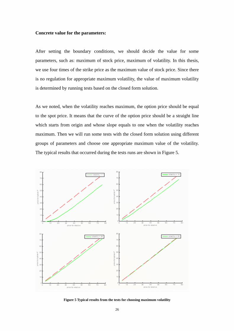
As we noted, when the volatility reaches maximum, the option price should be equal

to the spot price. It means that the curve of the option price should be a straight line

which starts from origin and whose slope equals to one when the volatility reaches

maximum. Then we will run some tests with the closed form solution using different

groups of parameters and choose one appropriate maximum value of the volatility.

The typical results that occurred during the tests runs are shown in Figure 5.

Figure 5 Typical results from the tests for choosing maximum volatility

26

From the tests, we can conclude that when volatility is equal to 40 or bigger the curve

of option price satisfies the requirement. Hence the maximum volatility for the finite

difference method will be set to 40.

Iteration Process

As mentioned in Section 5.1.2, central difference is applied for approximating the first

derivative with respect to price and volatility; formula (42) and (43) are given for

approximating the second derivative and the cross derivative with respect to

underlying asset or volatility; the Crank-Nicholson scheme is applied for solving the

ordinary differential equation. After necessary substitutions, a part of the Heston PDE

becomes as follow:

2 2 22 2

2 2

1 1, 2 1, 3 , 1 4 , 1 5 1, 1 6 ,

1 1( ( ) )2 2t t t t t t t

j k j k j k j k j k j k

u u u urS v S v v S v rus v s v

a u a u a u a u a u a u

κ θ λ σ σρ

+ − + − + +

∂ ∂ ∂ ∂+ − − + + + −

∂ ∂ ∂ ∂ ∂= + + + + +

us v∂∂ . (44)

where

21

22

2

3

2

4

5

22

6

1 12 21 12 2

( )2 2( )

2 2

2

a Nr MN v MN

a MN v Nr

M v M v Ma Mv v

M M v M vav v

a MN

Ma MN r MN vv

σρ

κ θ λ σ Nσρ

σ κ θ λ

σρ

σσρ

= + Δ −

= Δ −

− Δ − Δ= +

Δ Δ− Δ − Δ

= −Δ Δ

=

= − − Δ −

−

Δ

M and N are the number of how many steps of the price and volatility are divided

respectively. The index of price and volatility is represented by j and k respectively.

Expression (44) also could be expressed as matrix form:

,1M NAU b× +

27

max max

m

4 1, 0

6 3

4 6

3 1, 5 2,

4 2, 03

4 6

1 5

3 2,1

5

1

2

2

2

1 23 1

2,3 1

1

2

3

v

v v

v

v

A AA A

where AA

M N M NA A

a u

a aa a

a u a uAa ua

a a

a aa ua

A and baa

aa

A

a

=

=

⎛ ⎞⎜ ⎟⋅⎜ ⎟⎜ ⎟= ⋅ ⋅ ⋅⎜ ⎟

⋅ ⋅⎜ ⎟⎜ ⎟ × ×⎝ ⎠

⋅⎛ ⎞⎜ ⎟ ⋅⋅⎜ ⎟

+⎜ ⎟= ⋅ ⋅ ⋅⎜ ⎟

⋅ ⋅⎜ ⎟⎜ ⎟ ⋅⎝ ⎠

⋅⎛ ⎞⎜ ⎟⋅⎜ ⎟⎜ ⎟= =⋅ ⋅⎜ ⎟

⋅⎜ ⎟⎜ ⎟⎝ ⎠⎛ ⎞⎜ ⎟⎜ ⎟⎜ ⎟= ⋅⎜ ⎟

⋅⎜ ⎟⎜ ⎟⎝ ⎠

ax max

max max

max max

max max

max max max max

5 3,

1 ,1 5 ,2 4 , 0

1 ,2 5 ,3

1 ,3 5 ,4

1 , 3 , 5 ,

v

s s M v

s s

s s

s N M v s v

N

N

a u

a u a u a u

a u a u

a u a u

a u a u a u

=

⎛ ⎞ ⎫⎜ ⎟ ⎪

⎪⎜ ⎟⎬⎜ ⎟⎪⎜ ⎟⎪⎜ ⎟ ⎭

⎜ ⎟⎫⎜ ⎟⎪⎜ ⎟ ⎪⎜ ⎟ ⎬

⎜ ⎟ ⎪⎜ ⎟+ ⎪⎭⎜ ⎟

⋅⎜ ⎟ ⎫⎜ ⎟ ⎪⋅ ⎬⎜ ⎟

⎪⋅⎜ ⎟ ⎭⎜ ⎟+ +⎜ ⎟ ⎫⎜ ⎟ ⎪+⎜ ⎟ ⎪⎜ ⎟+ ⎪⎜ ⎟ ⎬

⋅⎜ ⎟ ⎪⎜ ⎟ ⎪⋅⎜ ⎟⎜ ⎟+ + ⎭⎝ ⎠

M N

N

⎫⎪⎪⎪⎪⎪⎪⎪⎪⎪⎪⎪⎪ ×⎬⎪⎪⎪⎪⎪⎪⎪⎪⎪⎪⎪

⎪ ⎪⎭

With the matrix form substituted in and the Crank-Nicholson scheme applied, the

Heston PDE becomes:

11 1

1 1

1 1( ) ( )2 2

2 2( ) ( ) (

i ii i i i

i i

u u Au Au b bt

A I u A I u b bt t

−− − 0

)i i− −

−+ + + + =

Δ

⇒ − = − + − +Δ Δ

. (45)

where i represents the index of time direction, tΔ is the time step, I is a

M N by M N× − − × identity matrix.

Subsequently, the option price will be calculated iteratively from time maturity to zero

time. Since A is a matrix with many zero elements, the LU factorization will be

used for solving the linear system.

28

5.3 Results In this section, the results obtained from the closed form solution and the finite

difference method will be discussed and compared; convexity will also be discussed

based on the results.

5.3.1 Results from the closed form solution

In this section, I will present the closed form solution graphically. Furthermore,

inappropriate parameter choice will also be given and discussed. The convexity based

on the closed form solution will be discussed at last.

Results and parameter

First, we choose two groups of parameters based on [10].

max

max

20, 80, 0.1, 0.1, 0.04, 0, 0.5, 2, 220, 80, 0.2, 0.5, 0.02, 0.1, 0.3, 3, 2

K S r TK S r T

ρ θ λ σ κρ θ λ σ κ

= = = = − = = = = == = = = − = = = = =

Figure 6 Results from the close form solution

The left hand side of Figure 6 is the result from the first group parameter, the right

hand side of the figure is the result from second one. The pictures look nice and the

curve of the option price is convex for difference volatility value.

Next step, we try another group of parameters. It is almost the same with first one; the

only difference is negative value for the term κ .The results are shown in Figure 7.

29

max20, 80, 0.1, 0.1, 0.04, 0, 0.5, 2, 2K S r Tρ θ λ σ κ= = = = − = = = = − =

Figure 7 Results from the close form solution for negative κ

The left hand side of Figure 7 is the result when volatility equals to 2; the right hand

side is the result when volatility equals to 0.1. Now we can clearly see that when

volatility is 2, the price almost reaches the upper boundary. When volatility equals to

0.1, the price of option has negative value which is absolutely wrong. Those

performances in Figure 6 are unreasonable. It is probably because of the negative κ .

To verify my thought, we do tests using the first group of parameters. The results with

volatility equals to 0.1 and 2 are shown in Figure 8:

Figure 8 Results for the first two groups of parameters when volatility = 0.1 and 2

From Figure 8, we can see that the performances of option price when volatility

equals to 0.1 are normal. We argue that the unreasonable results are due to the

negative . κ

30

Now we analyse the unreasonable choice of κ from theoretical point of view. As

explained in Section 2.3.2, our volatility process has the form as follow:

2( )t t tdv v dt v dWκ θ σ= − + .

The artificial process 2

2

4tV σ= tB , where tB is a n-dimensional Bessel process, has

the form as follow:

2

4t tdV ndt V dWσ σ= + t .

If 2

4n κθσ

= is fulfilled, those two processes has similar performance near zero. First,

we have positive 2σ ; θ is also positive since it is long term mean for volatility

which is always positive. Hence when κ is negative, “n” will become negative

which is unreasonable. Based on above analysis, any negative value for the term κ

is not considered in other tests.

At last, we run the tests with many groups of appropriate parameters. The results are

similar as Figure 6. We can say that the results shown in Figure 6 are the typical

results. In all, the option price is convex based on the closed form solution with

appropriate parameter.

Convexity based on closed form solution

Above, we can graphically see that the price for European call option is convex. On

the other hand, we can show the convexity by illustrating the Γ .

Because, , the second order derivative of European call option with respect to spot

price is a density function, we can conclude that the Greek

Γ

Γ based on the closed

31

form solution for the Heston model is always positive. We can also obtain numerical

typical results for the density function of log-spot price which is shown in Figure 9:

Figure 9 Typical result of density function of log-spot price with different volatility

The numerical values are positive. Consequently, we can say that the convexity for

European call option based on the closed form solution for the Heston model is

preserved.

5.3.2 Results from the finite difference method

In the implementation part, we set the number of discretisation for the price and the

volatility direction as 20, time maturity is 2, time step is 0.1, and maximum volatility

is always 40 as claimed in Section 5.2.2. Other parameters, including , , , , , rρ θ σ κ λ ,

will have different combinations. We choose many groups of parameters, and the

typical results that occurred during the tests are shown in Figure 10:

32

max20, 80, 0.1, 0.1, 0.04, 0, 0.5, 2K S r ρ θ λ σ κ= = = = − = = = =

Figure 10 Typical results from FDM for different groups of parameters

The left hand side of Figure 10 is the picture with different volatilities. To illustrate

the trend of the option price clearly, we only show the option price with four numbers

of volatility. We could see that the curve of the option price is pulling up toward the

boundary option price as long as the volatility increasing, also the option price is

convex at least for those four volatility values. The right hand side of Figure 10 shows

more precisely. We can conclude that the option price is convex for any volatility

value between the interval [0, 40].

From the tests with different groups of parameters, it seems that the parameters

,r ρ , θ and σ do not effect the results so much, we could always get the typical

results as Figure 10. Also it is important to notice that:

(a) We did not change the sign of θ which is the long term mean for volatility. Since

there is no negative volatility, θ couldn’t be negative.

(b) The termλ always equals to 0.

There is no λ term in the Black-Scholes formula, because the risk is completely

eliminated there. However the volatility is not tradable in the Heston’s model, one

cannot make a perfect portfolio which is risk-free. Thus, we have a λ term which is

the market price of volatility risk in our model.

33

Next we have two groups of parameters with non-zero λ . The results obtained from

the parameters below are shown in Figure 11.

max20, 80, 0.1, 0.1, 0.04, 0.2, 0.5, 2K S r ρ θ λ σ κ= = = = − = = = =

Figure 11 Results from λ = 0.2

We can see that the result after adding market price of volatility risk is still nice, and

the option price is convex. We try larger market price of risk, the results obtained

from the parameters below are shown in Figure 12.

max20, 80, 0.1, 0.1, 0.04, 1, 0.5, 2K S r ρ θ λ σ κ= = = = − = = = =

Figure 12 Results from λ = 1

The result is still nice, convexity is preserved. There is slightly difference between

Figure 11 and Figure 12, but it is barely visible. Hence we give the numerical

comparison in Table 5.

34

Spot price

Option price with λ = 0.2, volatility = 2

Option price with λ = 1, volatility = 2

4 0.26642 0.12408 8 1.3578 0.92477 12 3.146 2.4526 16 5.5315 4.6661 20 8.4403 7.5134 24 11.66 10.726 28 15.073 14.157 32 18.614 17.73 36 22.246 21.4 40 25.944 25.137 44 29.691 28.923 48 33.477 32.747 52 37.292 36.6 56 41.131 40.474 60 44.989 44.367 64 48.864 48.274 68 52.752 52.192 72 56.652 56.12 76 60.561 60.056

Table 5 Typical results of numerical comparison for the option price with different λ

From Table 5, we can clearly see that all the option price with larger λ when

volatility equals to 2 is smaller to the one with smaller λ . This is the typical result

during the tests. We conclude that the option price decreases when the market price of

volatility risk increases. It also accords with the real situation.

The result for every group of parameters is nice and as expected. Based on all the

results obtained from the finite difference method, we can conclude that the price for

European call option is convex and increases when the volatility increases.

5.3.3 Comparison between the results of the previous sections

In order to test the accuracy of the finite difference method, we compare the results

obtained from the finite difference method and the closed form solution. The

comparisons will be illustrated graphically and numerically, also base on several

groups of parameters. Results from the first group of parameters are shown in Figure

13:

35

max20, 80, 0.1, 0.1, 0.04, 0, 0.5, 2K S r ρ θ λ σ κ= = = = − = = = =

Figure 13 Comparison of FDM and closed form solution

We can see that the results obtained from both methods are very close. For further

comparison to see the difference of results, a statistical concept which is called the

standard error regression (SER) is applied. We fix the volatility; calculate SER by

following expression:

2( ( , ) ( , ))

1

ni i

CFS t FDM ti

C S v C S vSER

n

−=

−

∑.

where and represent the option price obtained from the

closed form solution and the finite difference method respectively when spot price is

and fix volatility is . We calculate SER when volatility equals to 2, 4, 10 and 30

which are shown in Table 6.

( , )iCFS tC S v ( , )i

FDM tC S v

itS v

Volatility 2 4 10 30

SER 0.135 0.045 0.002 0.075 Table 6 Numerical comparison between FDM and closed form solution

In general, the smaller the SER value, the smaller the difference between FDM and

closed form solution. From Table 6, we can see that the differences between these two

36

methods are slight. This slight difference is typical result during all the tests. It

indicates that the finite difference method with Crank-Nicholson scheme works well

and our boundary condition choices are appropriate.

37

Chapter 6 Conclusion

In this article we show that the option price is convex in the underlying asset, for all

fixed times, in the case of convex contract functions for the Heston stochastic

volatility model, see Chapter 4. In chapter 2 we discuss different volatility models and

in Chapter 3 we derive the pricing PDE in the Heston model. We also illustrate the

results using numerical methods, see Chapter 5.

38

Reference:

[1] F. Black and M. Scholes, 1973. “The Valuation of Options and Corporate

Liabilities,” Journal of Political Economy. 81,637-654

[2] B. Dupire, 1994. “Pricing With a Smile,” Risk, Vol 7 (1), 18-20

[3] J. C. Hull and A. White, 1987. “The Pricing of Options on Assets with Stochastic

Volatilities,” Journal of Finance, 42, 281-300.

[4] L. O. Scott, 1987. “Option Pricing When the Variance Changes Randomly:

Theory, Estimation and an Application,” Journal of Financial and Quantitative

Analysis 22/22, 419-438

[5] S. L. Heston, 1993. “A Closed-form Solution for Options with Stochastic

Volatility with Applications to Bond and Currency Options,” The Review of Financial

Studies, 6(2), 327-343

[6] R. Riccardo, 1999. Book Title: “Volatility and Correlation: The perfect Hedge and

the Fox”

[7] J. C. Cox, E. Ingersoll and S. A. Ross, 1985. “A Theory of the Term Structure of

Interest Rates,” Econometrica, 53, 385-408

[8] L. C. G. Rogers and D. Williams, 2000. “Diffusion, Markov Processes, and

Martingales” –Volume two: Ito calculus. Cambridge University Press.

[9] J. C. Cox and Ross S. A, 1976. “ The Valuation of Options for Alternative

Stochastic Processes,” Journal of Financial Economics, 3, 145-166

39

[10] T. Kluge, 2002. “Pricing derivatives in stochastic volatility model using the finite

difference method”

[11] O. Reiss and U. Wystup, 2001. “Computing Option Price Sensitivities Using

Homogeneity,” Journal of Derivatives 9(2): 41-53

[12] http://www.xplore-stat.de/tutorials/stfhtmlnode47.html

[13] R. Sheppard. “Pricing Equity Derivatives under Stochastic Volatility”

[14] J. Hull and A. White 1996 “Hull and White on Derivatives: A Compilation of

Articles.” Risk Publication, ISBN: 1899332456

[15] Y. Z. Bergman, B. D. Grundy and Z. Wiener 1996 “General properties of option

prices” J. Finance 51, 1573-1610

[16] G. Winkler, 2001. “Option Valuation in Heston’s Stochastic Volatility Model

using Finite Element Methods.”

[17] E. Ekstron and J. Tysk, 2006. “Convexity preserving Jump Diffusion Models for

Option Pricing.”

40