convergent iterative schemes for time …€¦ · convergent iterative schemes ... bubble and dew...

MATHEMATICS OF COMPUTATIONVolume 75, Number 255, July 2006, Pages 1403–1428S 0025-5718(06)01832-1Article electronically published on February 24, 2006

CONVERGENT ITERATIVE SCHEMESFOR TIME PARALLELIZATION

IZASKUN GARRIDO, BARRY LEE, GUNNAR E. FLADMARK, AND MAGNE S. ESPEDAL

Abstract. Parallel methods are usually not applied to the time domain be-cause of the inherit sequentialness of time evolution. But for many evolution-ary problems, computer simulation can benefit substantially from time par-allelization methods. In this paper, we present several such algorithms thatactually exploit the sequential nature of time evolution through a predictor-corrector procedure. This sequentialness ensures convergence of a parallelpredictor-corrector scheme within a fixed number of iterations. The perfor-mance of these novel algorithms, which are derived from the classical alternat-ing Schwarz method, are illustrated through several numerical examples usingthe reservoir simulator Athena.

1. Introduction

Hydrocarbon flow in porous media is often approximated with a mathematicalmodel involving three coupled nonlinear evolution equations for the primary vari-ables of temperature, pressure, and molar masses, and tabulated values based onbubble and dew point curves for the secondary variables. Since this model is gen-erally too difficult to solve analytically, a simplified model is solved numerically bydecoupling the equations and discretizing them using finite volume in space andbackward Euler in time. The resulting nonlinear system of equations is then solvedusing the iterative Newton-GMRES algorithm [3], [4].

This is the overall structure of Athena, our current simulator for flow in porousmedia. The goal of Athena is to simulate a wide variety of flow scenarios withinreasonable accuracy, in reasonable computational time. However, to simulate real-istic problems, the standard numerical algorithms are unacceptably slow. Thus, itis necessary to develop faster, parallel algorithms.

The standard numerical approach is to sequentially solve each primary variableusing a fixed time-step determined by the smallest evolutionary time-scale for theprimary variables, even though the time-scales for these variables may be an orderof magnitude different. In particular, the time-scale for temperature and pressureis often an order of magnitude larger than that for the molar masses. Hence, thetemperature and pressure can be computed with larger time-steps. To mitigatethis time-step restriction, a common procedure is to compute the temperature andpressure with time-step ∆T, while substepping G times for the molar masses with

Received by the editor May 29, 2003 and, in revised form, April 20, 2005.2000 Mathematics Subject Classification. Primary 65N55, 65Y05; Secondary 65M55, 65M60.Key words and phrases. Alternating Schwarz, time parallelization, reservoir simulator, multi-

level, full approximation storage.

c©2006 American Mathematical SocietyReverts to public domain 28 years from publication

1403

License or copyright restrictions may apply to redistribution; see http://www.ams.org/journal-terms-of-use

1404 I. GARRIDO, B. LEE, G. E. FLADMARK, AND M. S. ESPEDAL

smaller time-step ∆TG . However, this substepping does not lead to acceptable com-

putation efficiency in a serial computing environment.The goal of this paper is to develop parallelization techniques for the substep

procedure, in order to speed up the computation. An ideal algorithm is one thatwould completely bypass the sequential nature of time evolution in a parallelizedsubstep march. But this would go against physics, and so, may lead to poor accu-racy. Hence, we propose a novel method, similar to the Parareal technique studiedin [1, 8, 2], that allows parallelization in the substep procedure and is also causal.Causality is obtained by using a coarser time-step in a predictor-corrector manner.Both the Parareal technique and this proposed method have a two-level structure,with the predictor step defined on the coarse time level and the corrector step de-fined on the fine level. The novelty in our approach is to decrease the time domainas the predictor-corrector progresses.

This paper is organized as follows. For background and self-containment, Sec-tion 2 describes the equations of hydrocarbon flow in porous media. Given theseequations, in Section 3, we review some of the existing parallel algorithms to handleevolution equations, and give a general description of a predictor-corrector (PC)algorithm for parallelizing time. This general description is given in terms of aniterative method for solving a lower block bidiagonal matrix. The details of thisPC algorithm are given in Section 4. In this section, the PC method is viewed as atwo-level scheme, where the coarse grid and fine grid procedures are respectively thepredictor and corrector steps. Section 4 further derives defect terms that modifythe predictor equations, introduces modifications to the PC algorithm that ensureconvergence within a fixed number of iterations, and analyzes the computationalefficiency of this two-level algorithm. Section 5 develops a multilevel extensionthat alleviates some of the load-balance issues of the two-level method. The in-tricacies of this extension are given, as well as a description of the computationalcosts for a cycle of this multilevel method. Numerical examples are presented inSection 6 to illustrate the performance of these algorithms. Finally, Section 7 givesthe conclusions of this work.

We note that this paper concentrates on the derivation and properties of thenumerical algorithm, avoiding unnecessary details of our compositional simulatorAthena. For further details on Athena, we refer the interested reader to [5], [9],[10], and [11].

2. Equations of hydrocarbon flow

We are interested in a multicomponent multiphase fluid flow in a porous mediaregion V with surface boundary S. The primary variables of interest are temperature(T ), water pressure (pw), and molar masses (Nν), for each component (ν) of themulticomponent multiphase fluid. The phases considered are oil (o), gas (g), andwater (w). The mathematical model for hydrocarbon flow in porous media involvesconservation laws for the molar masses and internal energy, and a water pressureequation. Conservation of molar mass for a flow through a porous media region Vis given by the integral relation

∂

∂t

∫V

mν dV +∫

V

∇ · mν = −∫

V

qν dV ,(2.1)

where qν is the source/sink for molar mass density component mν (molar mass Nν

is the volume integral of mν). Conservation of energy is enforced through the heat


CONVERGENT ITERATIVE SCHEMES FOR TIME PARALLELIZATION 1405

flow equation

∂

∂t

∫V

(ρu)dV −∫

S

(k∇T ) · dS = −∫

S

hρu · dS +∫

V

qdV ,(2.2)

where T is the temperature, k is the bulk heat conductivity, ρ is the density, andu is the internal energy. And, an equation for the water pressure is derived byimposing that the pore volume Vp be equal to the sum volume of all three fluidphases at all times, i.e.,

R = Vp −∑

l=g,o,w

V l

is zero at all times. This residual volume is a function of the water pressure pw, theoverburden pressure W , and each molar mass component Nν . Hence, a first-orderTaylor expansion of R(t + ∆t) about t, together with the chain rule applied to∂R(pw, W, Nν)/∂t, leads to the water pressure equation

(2.3)∂R

∂pw

∂pw

∂t+

nc∑ν=1

∂R

∂Nν

∂Nν

∂t= − R

∆t− ∂R

∂W

∂W

∂t.

Equations (2.1)–(2.3) are three coupled nonlinear differential systems. The pres-sure and molar masses are clearly coupled in (2.3). The temperature is coupledto the pressure and molar masses through its Jacobian. This Jacobian is also de-pendent on the rock temperature, which in reservoir simulation has a much lowervariation rate than the pressure and molar masses.

Now, to numerically solve this differential system, these equations are decoupledand discretized using finite volume in space and backward Euler in time. Thus,at each time-step interval, [Tn, Tn+1], three discrete Jacobian systems of the formA[n]∆x = f [n] are solved in sequential order. These systems are solved with aniterative Newton–Raphson method using, for example, preconditioned GMRES [3],[4]. In general, at each time-step these Jacobian matrices change after each Newtoniteration. But for the temperature equation, since its Jacobian matrix is majorizedby the rock temperature, its Jacobian will be changed only between each time-step.Having determined the temperature at time T [n+1], the pressure and molar massesmust be determined using a Newton–Raphson iteration. As for the pressure system,its Jacobian has off-diagonal terms that depend on the molar masses. Because ofthe decoupling, these off-diagonal terms will involve only time-lagged molar masses.Thus, the nonlinearities in the discrete pressure equation are restricted to the di-agonal terms A[n] = D[n(s)], where the superscript s corresponds to the numberof Newton iterations. Turning to the molar mass, as noted in Section 1, the rateof change for the temperature and pressure are comparatively small compared tothe rate of change for the molar masses. So, for each time-step interval, the molarmass equations are substepped with step-size T n+1−T n

G . Given the temperature andpressure, the nonlinear molar mass system at time-level Tn is

A[n(s)]( N [(n)(s+1)] − N [n(s)]) = f [n(s)].(2.4)

Superscript s will be omitted in the remainder of this paper.For further details of the discretization of (2.1)–(2.3), we refer the interested

reader to [7].



3. Parallel algorithms for evolutionary equations

In this section, we review some of the existing parallel algorithms for evolutionaryequations. As alluded to in the previous section, the most computationally intensiveprocedure in hydrocarbon flow simulation is the substep march for the molar masses.If this procedure can be computed in parallel, then the computation of the molarmasses can be substantially improved. In general, such parallelization can improvethe computational performance for any of the three variables.

The solution procedure for an evolutionary equation time-discretized with back-ward Euler can be viewed as a forward substitution (or an approximation) for thelower block bidiagonal matrix system⎛

⎜⎜⎜⎜⎜⎜⎜⎜⎝

L1

M1 L2

M2 L3

. . . . . .

MN−1 LN

⎞⎟⎟⎟⎟⎟⎟⎟⎟⎠

⎛⎜⎜⎜⎜⎜⎜⎜⎜⎝

u1

u2

u3

...

uN

⎞⎟⎟⎟⎟⎟⎟⎟⎟⎠

=

⎛⎜⎜⎜⎜⎜⎜⎜⎜⎝

f1

f2

f3

...

fN

⎞⎟⎟⎟⎟⎟⎟⎟⎟⎠

,(3.1)

where Li is the matrix operator acting on the unknown at the ith time-step andMi−1 is the matrix operator acting on the unknown of the previous time-step. Adirect forward substitution is clearly sequential in time. However, to achieve someparallelism, a common approach is to parallelize in space as time is sequentiallymarched. This corresponds to forward substituting (3.1) with parallelism in theinversion of Li. For example, when the evolutionary equation is parabolic, inversionof Li corresponds to solving an elliptic equation, in parallel. This standard approachdefinitely does not exploit full parallelism, especially when the temporal grid is muchfiner than the spatial grid.

Two other parallel approaches for time-dependent problems are waveform re-laxation and overlapping Schwarz waveform relaxation. These methods do achieveparallelism in time. To describe these approaches, consider a one-dimensional time-dependent problem, i.e., 1-1 dimensional in space-time. Spatially discretizing thisproblem leads to a system of ode’s, one equation for each spatial grid point:

du

dt+ Au = f,(3.2)

where A is the matrix that describes the coupling produced by the spatial dis-cretization. Denoting the diagonal of A with D, a Jacobi-type iterative scheme forsolving (3.2) is

duk

dt+ Duk = f + (D −A)uk−1,(3.3)

which leads to a system of decoupled ode’s at each iteration. Each of these time-dependent problems is then solved for the complete time interval on different CPU’s.This is the basic waveform relaxation approach. A generalization of it is the over-lapping Schwarz waveform scheme ([6]). Rather than subdividing the spatial do-main with grid points, the overlapping Schwarz method decomposes the spatialdomain into several overlapping subdomains; see Figure 1. On each subdomain, atime-dependent problem must be solved. These subdomain problems are solved in



time

space

1ΩΩ0

1Ω

U

0Ω

Figure 1. Domain decomposition for the overlapping Schwarzwaveform method.

parallel, with an appropriate strategy for updating the subdomain interface values.

Waveform relaxation suffers from poor convergence. Hence, several multigridschemes have been developed by Vandewalle et al. ([14]) to overcome this conver-gence problem. Overall, this scheme can be viewed as applying multigrid to a fullydiscretized time-dependent problem, with time viewed as another spatial variable.However, because the space-time grid is generally anisotropic (e.g., ∆t ∆x),line relaxation or semi-coarsening must be used in the multigrid procedure ([13],[15]). For our 1-1 dimensional problem, line relaxation in the time direction, asthe strength of connection is in the time direction when ∆t ∆x, is equivalentto solving a one-dimensional evolutionary equation. The solving of this line is per-formed using cyclic reduction, which can be done recursively in a multigrid fashionand in parallel. Vandewalle et al. has also examined semi-coarsening and pointwisesmoothing, which lead to better parallelism.

The above parallel approaches have been most successfully applied to second-order parabolic equations. However, for hyperbolic systems, the smoothing char-acteristic of parabolic equations is not present, and so, the overlapping Schwarzand multigrid methods may suffer. Moreover, for higher-dimensional equations,algorithmic/implementation issues can make these methods impractical.

Before introducing an alternative approach, it is insightful to examine the cyclicreduction scheme for solving (3.1). Cyclic reduction is a direct method that com-bines the even numbered equations with the odd numbered equations to create asystem half the original size and with the same bandwidth pattern. For example,when N = 8 in (3.1), the reduced system is

⎛⎜⎜⎜⎜⎜⎜⎜⎜⎜⎝

L2

− M3L−13 M2 L4

−M5L−15 M4 L6

−M7L−17 M6 L8

⎞⎟⎟⎟⎟⎟⎟⎟⎟⎟⎠

⎛⎜⎜⎜⎜⎜⎜⎜⎜⎜⎝

u2

u4

u6

u8

⎞⎟⎟⎟⎟⎟⎟⎟⎟⎟⎠

=

⎛⎜⎜⎜⎜⎜⎜⎜⎜⎜⎝

f2 − M1L−11 f1

f4 − M3L−13 f3

f6 − M5L−15 f5

f8 − M7L−17 f7

⎞⎟⎟⎟⎟⎟⎟⎟⎟⎟⎠

.



The solution components of the smaller system and original system are the same,and this size reduction procedure can be repeated recursively until a small systemthat can be easily solved is formed. Once the solution of the smallest system hasbeen determined, it can be used to calculate the unresolved values of the next largersystem. This back substitution procedure is recursively applied up to the originalsystem. Of course, a problem is the inversion of Li’s when they are submatrices, as isthe case in higher-dimensional evolutionary equations. Nevertheless, this proceduregives insight into developing other methods.

One can view the above procedure as initially “ignoring” the odd numbered un-knowns and modifying the original system to account for this ignoring. Supposethat instead of ignoring and modifying, approximations to the odd numbered com-ponents can be computed. Then with these values, the following reduced systemcan be formed:⎛

⎜⎜⎜⎜⎜⎝

L2

L4

L6

L8

⎞⎟⎟⎟⎟⎟⎠

⎛⎜⎜⎜⎜⎜⎝

u2

u4

u6

u8

⎞⎟⎟⎟⎟⎟⎠ =

⎛⎜⎜⎜⎜⎜⎝

f2 −M1u1

f4 −M3u3

f6 −M5u5

f8 −M7u7

⎞⎟⎟⎟⎟⎟⎠ ,(3.4)

where ui denotes an approximation to ui. In fact, this reduction can be done in acoarser fashion. For example, suppose only an approximation to u4 is known. Thenthe reduced or decoupled system is

(3.5)⎛⎜⎜⎜⎜⎜⎜⎜⎜⎜⎜⎜⎜⎜⎜⎜⎜⎜⎜⎜⎜⎜⎜⎜⎜⎝

⎡⎢⎢⎢⎢⎢⎢⎢⎢⎢⎣

L1

M1 L2

M2 L3

M3 L4

⎤⎥⎥⎥⎥⎥⎥⎥⎥⎥⎦

⎡⎢⎢⎢⎢⎢⎢⎢⎢⎢⎣

L5

M5 L6

M6 L7

M7 L8

⎤⎥⎥⎥⎥⎥⎥⎥⎥⎥⎦

⎞⎟⎟⎟⎟⎟⎟⎟⎟⎟⎟⎟⎟⎟⎟⎟⎟⎟⎟⎟⎟⎟⎟⎟⎟⎠

⎛⎜⎜⎜⎜⎜⎜⎜⎜⎜⎜⎜⎜⎜⎜⎜⎜⎜⎜⎜⎜⎜⎜⎜⎜⎜⎜⎜⎝

u1

u2

u3

u4

u5

u6

u7

u8

⎞⎟⎟⎟⎟⎟⎟⎟⎟⎟⎟⎟⎟⎟⎟⎟⎟⎟⎟⎟⎟⎟⎟⎟⎟⎟⎟⎟⎠

=

⎛⎜⎜⎜⎜⎜⎜⎜⎜⎜⎜⎜⎜⎜⎜⎜⎜⎜⎜⎜⎜⎜⎜⎜⎜⎜⎜⎜⎝

f1

f2

f3

f4

f5 − M4u4

f6

f7

f8

⎞⎟⎟⎟⎟⎟⎟⎟⎟⎟⎟⎟⎟⎟⎟⎟⎟⎟⎟⎟⎟⎟⎟⎟⎟⎟⎟⎟⎠

.

Each subblock is lower bidiagonal, and so, if approximations to some of the subblockunknowns are available, then this procedure can be applied recursively. Moreover,because the subblocks are decoupled, each subblock system can be performed inparallel. Naturally, since only approximate values for the lower subblocks are used,this procedure must be repeated iteratively. This is the essence of the novel parallelmethod we propose.

4. A two-level algorithm—the general scheme

So the idea of our parallel method is to compute approximations to the solutionat certain time levels. These approximations will permit the time march to decou-ple over subintervals, which in turn, will lead to parallelization of the march overthe whole time interval. To compute these approximations, a predictor-correctorprocedure is used. But unlike a typical predictor-corrector (PC) method, where anexplicit scheme predicts the solution at a fixed time and an implicit method corrects



Figure 2. The solution over the total coarse domain (in the left)determines the BCs for each parallel-fine system.

the prediction, in our method, the solution is both predicted and corrected withbackward-Euler, at a collection of time levels, and with the corrector computed inparallel. The difference between our predictor and corrector procedures lies in thesize of the time-steps, since the predictor uses a coarse step whereas the correctoruses a fine step. Thus, the overall parallel procedure can be viewed somewhat as afull approximation storage (FAS) multilevel scheme [13]. We describe this methodcorresponding to matrix equation (3.4) first.

Consider the domain Ω = Γ ∪ Ω as shown in Figure 2, where Γ = Tn denotesthe boundary where the initial boundary condition is given and Ω = (Tn, Tn+1].The diameter ∆T = (Tn+1 − Tn) of Ω can be viewed as the time-step for thetemperature and pressure equations in the hydrocarbon flow model. Recall thatthe target temporal grid for the molar mass equations has mesh size ∆t = ∆T

G .Besides Ω and the target temporal grid, we introduce an intermediate grid obtainedby subdividing Ω into P subdomains Ωi with mesh size ∆P = p∆t. Hence, Ω =⋃P

i=1 Ωi, Ωi = (Tn + (i− 1)∆P, Tn + i∆P ], and G = Pp. For example, in Figure 2,we have P = 4, p = 1, and G = 4, whereas in Figure 3, P = 3, p = 4 andG = 12. Subdomains Ωi for i > 1 have interface boundaries Γi, and Ω1 has theactual boundary Γ1 = Γ. Also, inside each subdomain, different discretizationsthat appropriately match along the interfaces can be used, though we opt to usethe same backward Euler and finite volume discretizations in each subdomain. Wenow have the multilevel grid hierarchy for the algorithm.

Consider the two-level grid setup of Figure 2. In this predictor-corrector algo-rithm, we alternatively solve over the entire coarse domain Ω (predictor) and in thenonoverlapping fine subdomains (corrector). Let N [n] denote the initial boundarycondition (BC) at time Tn. Tracking the predictor-corrector iterate with k, in thecoarse domain, the residual boundary value problem (BVP) is

(4.1)A[n],k∆u[n],k = f [n],k Ω,

u[n],k|Γ = N [n] Γ ,



where ∆u[n],k = u[n+1],k − u[n],k. Having solved this BVP, the initial conditionu

[n],k|Γ = u

[n],k|Γ1

= N [n] together with some approximations to the interface val-

ues u[n],k|Γi

, i = 2, . . . , P, serve as initial conditions for the subdomain problems to

be solved in parallel. These interface approximations, g[n],ki , can be obtained by

linearly interpolating u[n],k and the computed solution u[n+1],k, or they can be con-structed explicitly with a substep march over the intermediate grid if p > 1 inthe grid setup. In either case, solving equation (4.1) is the predictor step, whichdetermines boundary conditions for the fine subdomain systems

(4.2)A[n],k

i ∆u[n],ki = f

[n],ki Ωi

u[n],ki|Γi

= g[n],ki Γi

i = 1, . . . , P.

Note that subdomain Ω1 is also solved on the fine grid.Now, having solved (4.2) in parallel, their solutions provide a correction to the

coarse predictor system. Several choices for this correction will be given in the nextsubsection. Letting S denote this correction, the overall predictor-corrector cyclecan be viewed as a block Gauss-Seidel iteration: the predictor step sequentiallysolves the entire time-domain using correction S constructed from the previouscorrector solution, and the corrector step immediately uses the predictor solutionto determine the interface boundary values.

Iterate

• on processor 0 solve

(4.3) A[n],k|Ω ∆u

[n],k|Ω = f [n],k + S [n],k −A[n],k

|Γ N [n];

• on processor i, i = 1, . . . , P, solve

(4.4) A[n],ki|Ωi

∆u[n],ki|Ωi

= f[n],ki −A[n],k

i|Γig[n],ki .

There are many strategies for determining when this alternating method hasconverged. Due to the solution smoothness in time, we stop this alternating it-eration when the solutions of (4.3) and (4.4) at i = P differ within some giventolerance, e.g., the tolerance can be O(∆T − ∆t), the difference between the orderof the coarse and fine time discretizations.

4.1. Correction terms. To derive a correction term for the predictor equation, weestablish a relation between the predictor and corrector solutions. To accomplishthis, we assume a multilevel grid setup with p > 1, i.e., the intermediate subdomainpartitioning and the target fine grid are different. With this setup, equation (4.1)can be solved with a substep march over the subdomain partitioning. Such amarch will then explicitly determine the interface boundary conditions for the finecorrector equations, instead of linearly interpolating them from u[n],k and u[n+1],k.Hence, the BVPs

(4.5)A[n],k

|Ωi∆u[n],k = f

[n],k

|Ωi

u[n],k|Γi

= N [n] +∑i−1

j=1 ∆u[n],k|Ωj

i = 1, . . . , P,

are sequentially solved in the predictor procedure. Moreover, because p > 1, asubstep march must also be conducted in the corrector procedure. Indexing the



substeps in subdomain Ωi by i(j), these fine corrector equations are

(4.6)A[n],k

i|Ωi(j)∆u

[n],ki(j) = f

[n],k

i|Ωi(j)

u[n],ki|Γi(j)

= u[n],ki|Γi(1)

+∑j−1

l=1 ∆u[n],ki|Ωi(l)

⎫⎬⎭ j = 1, . . . ,

with interface boundary condition ui|Γi(1)= gi.

To establish a relation between the predictor and corrector solutions, we addand subtract A[n],k−1

|Ωi∆u

[n],k−1

|Ωifrom the first equation of (4.5) to get

(4.7) ∆u[n],k−1

|Ωi= ∆u

[n],k−1

|Ωi+ (A[n],k−1

|Ωi)−1(A[n],k

|Ωi∆u[n],k − f

[n],k

|Ωi).

Expanding ∆u[n],k−1

|Ωi, (4.7) is equivalent to

(4.8) u[n],k−1|Γi+1

= u[n],k−1|Γi+1

+ (A[n],k−1

|Ωi)−1(A[n],k

|Ωi∆u[n],k − f

[n],k

|Ωi).

Since corrector system (4.6) is solved more accurately over Ωi than in the predictormarch, we substitute u

[n],k−1|Γi+1

on the right-hand side of (4.8) with u[n],k−1i|Γi+1

:

u[n],k−1|Γi+1

= u[n],k−1i|Γi+1

+ (A[n],k−1

|Ωi)−1(A[n],k

|Ωi∆u[n],k − f

[n],k

|Ωi) ,

or equivalently,

(4.9) A[n],k

|Ωi∆u[n],k = f

[n],k

|Ωi+ A[n],k−1

|Ωi(u[n],k−1

|Γi+1− u

[n],k−1i|Γi+1

) .

Equation (4.9) is the corrected predictor equation we solve on the coarse grid to getthe interface value u

[n],k|Γi+1

for the corrector equation. Note that due to the nonlin-

earity of the molar mass system, the correction term A[n],k−1

|Ωi(u[n],k−1

|Γi+1−u

[n],k−1i|Γi+1

) isalso nonlinear, and hence, must be updated at every Newton iteration.

Another correction scheme can be derived by adding and subtracting all earlierpredictor-corrector iterates to (4.8) and using the more accurate u

[n],ji|Γi+1

’s:

(4.10) A[n],k

|Ωi∆u[n],k = f

[n],k

|Ωi+

k−1∑j=1

A[n],j

|Ωi(u[n],j

|Γi+1− u

[n],ji|Γi+1

) .

This is the Parareal correction term proposed by Maday and Lions ([1], [8], [2]).For weakly nonlinear problems, a modification of this Parareal correction term is

(4.11) A[n],k

|Ωi∆u[n],k = f

[n],k

|Ωi+ A[n],k

|Ωi

k−1∑j=1

(u[n],j|Γi+1

− u[n],ji|Γi+1

) .

The implementation and computation of this latter correction term is greatly sim-plified because only the current matrix operator has to be formed.

Yet another correction scheme follows naturally by reformulating the PC schemeas a two-level FAS method [13]. In each of the above correction terms, the operatorA[n],j

|Ωiis applied to the difference of a predictor solution and a corrector solution.

Alternatively, a correction term can be formed using the operators of the two time-levels and only the more accurate corrector solution:[

A[n],k−1

|Ωi−A[n],k−1

i|Ωi(p)

]u

[n],ki|Γi+1

,(4.12)



giving the corrected predictor equation

A[n],k

|Ωi∆u[n],k = f

[n],k

|Ωi+

[A[n],k−1

|Ωi−A[n],k−1

i|Ωi(p)

]u

[n],ki|Γi+1

.(4.13)

Correction term (4.12) can be viewed as an approximation to the local truncationerror at time Γi+1, which is the term that must be added to the right-hand side ofthe predictor equation to produce a coarse grid solution with fine grid discretizationaccuracy [13].

4.2. Improved parallel PC algorithm. Employing any of the correction termsgiven in (4.9)–(4.11) and (4.13), we have a parallel PC algorithm. The accuracyof this method is determined by the accuracy of the corrector procedure. Eachiteration consists of first solving over the whole coarse time interval and then asyn-chronously solving over each subdomain. However, causality implies that the solu-tion in the initial subdomain is not affected by the solution time subdomains at alater time. This observation permits a simple modification of the PC scheme thatensures convergence within P iterations. The idea is to decrease the active timeinterval by removing the initial subdomain after each PC iteration. In particular, inthe first PC iteration, since both the predictor and corrector solve the same initialboundary-value problem in subdomain Ω1, and since the solution in this subdomainis physically unaffected by the solution in the later subdomains, one can take themore accurate fine-grid corrector approximation to be the solution in Ω1. Havingdetermined the solution in Ω1, this subdomain can be eliminated from the activetime interval:

(4.14) Ωactive = Ω/Ω1 .

For the next PC iteration, on initial subdomain Ω2 of the current Ωactive, thecomputed fine grid solution u

[n],11|Γ2

will be taken as the initial condition

(4.15) u[n],2|Γ2

= u[n],11|Γ2

.

Figure 3. Active domain for the improved PC algorithm.



Although the right-hand side of the predictor equation in Ω2 now has a nonzerocorrection term, the actual equation being solved is the fine-grid corrector equation.Besides, the correction term in the predictor equation is used only to generateaccurate subdomain interface conditions for the corrector systems (cf. Section 5.1concerning the correction term 4.13). Hence, again we take the more accuratefine-grid corrector approximation in Ω2, and redefine the active time interval toΩactive = Ω/

⋃2i=1 Ωi. After repeating this process k = P − 1 times, the computed

solution at the Γi’s will be

(4.16) u[n],P|Γ1

= g, . . . , u[n],P|ΓP

= u[n],P−1P−1|ΓP

,

and the active time interval will be Ωactive = Ω/⋃P−1

i=1 Ωi. At this stage of the PCiteration, both the predictor and corrector equations have the same initial conditionand are defined only over ΩP . Once again the fine-grid corrector approximation istaken to be the solution in ΩP . Thus, after at most P iterations, this improvedalgorithm converges with accuracy determined by the corrector approximations. Agraphic overview of how the active time domain evolves as the method progressesis shown in Figure 3.

Algorithm: Improved PC Algorithm

• Ω =⋃P

i=1 Ωi, Ωi =⋃p

j=1 Ωi(j).

• g = N [n], S1 = 0.• For k = 1, . . .

– Solve sequentially at processor root for i = k, . . . , P , where S[n],k

|Ωiis

given in (4.9), (4.10) or (4.11)

(4.17)

A[n],k

|Ωi∆u[n],k = f

[n],k

|Ωi+ S

[n],k

|Ωi,

u[n],k|Γi

= u[n],k|Γi−1

+ ∆u[n],k

|Ωi−1, i > k,

u[n],k|Γ = g , i = k = 1,

u[n],k|Γi

= u[n],k−1i−1|Γi

, i = k > 1,

– At each ith-processor with gi = u[n],k|Γi

, i = k, . . . , P , solve sequentially

for j = 1, . . . , p

(4.18)

A[n],k

i|Ωi(j)∆u

[n],ki = f

[n],k

i|Ωi(j),

u[n],ki|Γi(j)

= u[n],ki|Γi(j−1)

+ ∆u[n],k

i|Ωi(j−1), j > 1,

u[n],ki|Γi(j)

= gi , j = 1,

– Modify the active time domainΩ ← Ω/Ωk,

If ‖u[n],kP |ΓP+1

− u[n],k|ΓP+1

‖ ≤ tol or k = P, stop.

Remark. The goal of our two-level PC scheme is to reach convergence in far fewerthan P iterations, otherwise the parallel fine-grid corrector procedure would havebenefited little, and this PC iteration would be forward substitution. In termsof matrix system (3.1), this improved PC iteration is an “iterative forward sub-stitution” method for solving a block lower bidiagonal system. Our numericalexperiments demonstrate that fewer than P iterations are needed.



4.3. Linearized PC algorithm. So far, our PC scheme has been developed usinga coarse substep march to generate the interface boundary conditions. It is verytentative to derive these interface conditions by linearly interpolating u[n],k andu[n+1],k. This would eliminate the need to substep on the coarse temporal grid,and thus, reduce the computational cost. Such an interpolation approach wouldbe suitable for linear and weakly nonlinear problems. However, for highly nonlin-ear problems, because linear interpolation may poorly approximate the nonlinearnature of the system, the required number of iterations for this “linearized” PCscheme will generally be more than that for the scheme of Section 4.2, thoughstill within P iterations. Nevertheless, at the kth iteration of this PC scheme, thelinearly interpolated interface conditions are

gi =P − i + 1P − k + 1

u[n],k|Γ +

i − k

P − k + 1u

[n],k|ΓP+1

, i = k, . . . , P,

where Γ is the left boundary of the active time domain, and the modified correctedpredictor equations are

A[n],k

|Ω ∆u[n],k = f[n],k

|Ω + A[n],k−1

|Ω (u[n],k−1|ΓP+1

− u[n],k−1P |ΓP+1

) ,(4.19)

A[n],k

|Ω ∆u[n],k = f[n],k

|Ω +k−1∑j=1

A[n],j

|Ω (u[n],j|ΓP+1

− u[n],jP |ΓP+1

) ,(4.20)

A[n],k

|Ω ∆u[n],k = f[n],k

|Ω + A[n],k

|Ω

k−1∑j=1

(u[n],j|ΓP+1

− u[n],jP |ΓP+1

) .(4.21)

Remark. Although the interface conditions and correction terms involve linearlyinterpolated values, at each Newton iteration, the A[n],k

|Ω ’s must be updated, i.e.,they are not linearized.

Algorithm: Linearized PC Algorithm

• Ω =⋃P

i=1 Ωi, Ωi =⋃p

j=1 Ωi(j).

• g = N [n], S1 = 0,• For k = 1, . . . ,

– Solve sequentially at processor root over the active domain Ω, whereS[n],k is given by (4.19), (4.20), or (4.21):

(4.22)A[n],k

|Ω ∆u[n],k = f[n],k

|Ω + S[n],k

|Ω ,

u[n],k|Γ = g , k = 1,

u[n],k|Γ = u

[n],k−1k−1|Γk

, k > 1,

– At each ith-processor with gi = P−i+1P−k+1

u[n],k|Γ + i−k

P−k+1u

[n],k|ΓP+1

,,

i = k, . . . , P, solve sequentially for j = 1, . . . , p

(4.23)

A[n],k

i|Ωi(j)∆u

[n],ki = f

[n],k

i|Ωi(j),

u[n],ki|Γi(j)

= u[n],ki|Γi(j−1)

+ ∆u[n],k

i|Ωi(j−1), j > 1,

u[n],ki|Γi(j)

= gi , j = 1.

– Modify the active time domainΩ ← Ω/Ωk.

If ‖u[n],kP |ΓP+1

− u[n],k|ΓP+1

‖ ≤ tol or k = P, stop.



4.4. Two-level computational efficiency. A deficiency in the two-level methodof Section 4.2 is the bottleneck in (4.17). For each PC iteration, the root processormust complete its sequential march before the child processors can start, resultingin processor idleness and communication traffic. The bottleneck in processor com-munication can be mitigated by looping (4.17) and (4.18) differently:

Algorithm: Reduced Bottleneck Loop

For k = 1, . . .For i = k, . . . , P − 1,

– Solve at processor root

(4.24)A[n],k

|Ωi∆u[n],k = f

[n],k

|Ωi+ S

[n],k

|Ωi,

u[n],k|Γi

= u[n],k|Γi−1

+ ∆u[n],k

|Ωi−1, i > k,

u[n],k|Γi

= u[n],k−1i−1|Γi

, i = k.

– At processor (i + 1), with gi+1 = u[n],k|Γi+1

, begin solving for

j = 1, . . . , p

(4.25)

A[n],k

i+1|Ω(i+1)(j)∆u

[n],ki+1 = f

[n],k

i+1|Ω(i+1)(j),

u[n],ki+1|Γ(i+1)(j)

= u[n],ki+1|Γ(i+1)(j−1)

+ ∆u[n],k

i+1|Ω(i+1)(j−1), j > 1,

u[n],ki+1|Γ(i+1)(j)

= gi+1 , j = 1.

Solve subdomain i = P on the root processor

(4.26)A[n],k

|ΩP∆u[n],k = f

[n],k

|ΩP+ S

[n],k

|ΩP,

u[n],k|ΓP

= u[n],k|ΓP−1

+ ∆u[n],k

|ΩP−1, i > k.

Now once the root processor has finished a substep, it can immediately communicatethe computed interface boundary condition to the appropriate child processor, and,while this communication is occurring, the root processor can begin its next substep.As for processor idleness, it can be reduced by starting the next predictor cycle onthe child processors that have completed their marches before the root processor hascompleted its march. This unfortunately involves complicated processor scheduling.

Suppressing this complicated scheduling, the efficiency of the parallel two-levelmethod can be obtained by counting specific substep solves on all processors, andcounting the number of blocking communications (i.e., communications that delaythe start-up of the last running processor1). In particular, substeps that are solvedconcurrently on different processors are counted only once. This is illustrated inFigure 4, which shows the counts for three different subdomain partitionings of afine grid with G = 16, e.g., for the top partitioning, since the first subdomain ofboth levels are solved concurrently, they are numbered 1, since the second substepof both levels and the ninth substep of the fine level are all solved concurrently, theyare numbered 2, etc. Table 1 summarizes the efficiency for several time-marchingschemes. First, a serial march requires no communication and only G substeps sincethe predictor is not needed. For the two-level method with loops (4.17)–(4.18), inthe kth PC iteration, (P − k + 1) substeps are needed for the predictor and psubsteps are needed for the corrector. Moreover, before the last processor can start

1The root processor can communicate each interface value using point-to-point communica-tions, or it can communicate all the interface values at once using a scatter communication. Forlarge sets of data, both types of communication complete their tasks in about the same time.



1 2

1 2 3 4 5 6 7 8 2 3 4 5 6 7 8 9level 1

level 0

1 2 3 4

1 2 3 4 2 3 4 5 63 4 5 4 5 6 7

level 1

level 0

5

2 31 4 5 6 7 8

1 22 3 3 4 4 5 5 6 6 7 7 8 8 9

level 1

level 0

Proc 0

Proc 2Proc 1

Proc 1 Proc 2 Proc 3 Proc 4

Proc 0

Proc 2Proc 1 Proc 3 Proc 4

Tn

Tn+1/4

Tn+1/2

Tn+3/4

Tn+1


Proc 0

Figure 4. Two-level Method. Counting the substep solves inthe first PC iteration for three different subdomain partitionings:G = 16, (P, p) = (2, 8), (4, 4), (8, 2). Substep solves that occur si-multaneously on different processors are counted only once.

its march, it must wait for (P − k) communications. Hence, for l iterations, theefficiency of this scheme is

l∑k=1

[(P − k + 1 + p) solves + (P − k) comms]

= l

(P + p + 1 − (l + 1)

2

)solves + l

(P − l + 1

2

)comms.

Finally, using the above counting convention, in the kth PC iteration, the two-levelmethod with loop (4.24)–(4.25) requires (P −k+p) solves. Also, since the predictormarch continues while communication is occurring, only the last communication isblocking. Thus, for l iterations, the efficiency of this scheme is

l∑k=1

[(P − k + p) solves + 1 comms] = l

(P + p − (l + 1)

2

)solves + l comms.

Table 1. Efficiency for the kth iteration. The serial method per-forms only 1 iteration, a forward substitution.

Method SubSteps Comms Efficiency

serial G none G substepsLoops (4.17)–(4.18) (P − k + 1 + p) (P − k) (P − k + 1 + p) substeps & (P − k) commsLoop (4.24)–(4.25) (P − k + p) (P − k) (P − k + p) substeps & 1 comm



Note that irrespective of the subdomain partitioning, the two-level method withloop (4.24)–(4.25) requires just 1 blocking communication. Thus, its efficiency atthe kth iteration is optimized by choosing a partition that minimizes the substepcount. That is, its efficiency is optimized by minimizing

f(P ) = P − k + p = P − k +G

P.

The minimum of f occurs at P =√

G, and the minimal value is (2√

G−k). Hence,this two-level scheme’s optimal efficiency for l iterations is

l

(2√

G − (l + 1)2

)solves + l comms.

But obviously this choice for P affects the value of l, the required number of PCiterations to reach convergence.

5. Multilevel extensions

A remaining issue with the two-level method is processor idleness. This problemcan be further embellished when the optimal subdomain partitioning is chosen,since then only (

√G + 1) of the total number of processors are used. Hence, there

is an incentive for having many small subdomains. In this section, we develop amultilevel extension of the two-level method that uses just such partitioning yetkeeps the substep count low.

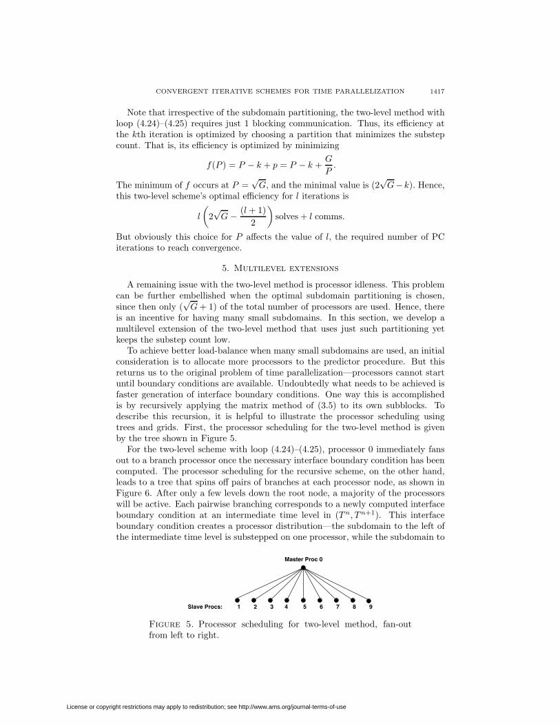
To achieve better load-balance when many small subdomains are used, an initialconsideration is to allocate more processors to the predictor procedure. But thisreturns us to the original problem of time parallelization—processors cannot startuntil boundary conditions are available. Undoubtedly what needs to be achieved isfaster generation of interface boundary conditions. One way this is accomplishedis by recursively applying the matrix method of (3.5) to its own subblocks. Todescribe this recursion, it is helpful to illustrate the processor scheduling usingtrees and grids. First, the processor scheduling for the two-level method is givenby the tree shown in Figure 5.

For the two-level scheme with loop (4.24)–(4.25), processor 0 immediately fansout to a branch processor once the necessary interface boundary condition has beencomputed. The processor scheduling for the recursive scheme, on the other hand,leads to a tree that spins off pairs of branches at each processor node, as shown inFigure 6. After only a few levels down the root node, a majority of the processorswill be active. Each pairwise branching corresponds to a newly computed interfaceboundary condition at an intermediate time level in (Tn, Tn+1). This interfaceboundary condition creates a processor distribution—the subdomain to the left ofthe intermediate time level is substepped on one processor, while the subdomain to

Master Proc 0

Slave Procs: 1 2 3 4 5 6 7 8 9

Figure 5. Processor scheduling for two-level method, fan-outfrom left to right.



0

1

12

2

543

7 8 9 10 11 13 14

1615 17 18 19 20 21 22 23 24 2625 27 28 29 30

6

Figure 6. Processor scheduling for the multilevel method.

the right is substepped on another processor. Figure 7 elaborates this branching.In this diagram, there are three coarsenings of the bottom target grid. For thetwo-level method, the bottom grid and any one of the other three grids, dependingon the subdomain partitioning, are used. For the recursive multilevel scheme, thecollection of all the grids forms the multilevel grid hierarchy. Corresponding tothis grid hierarchy is a processor distribution. Each processor takes a subdomaincomposed of two substeps. For example, Proc 0 takes the top grid with the wholetime domain [Tn, Tn+1] as one subdomain with two substeps, Proc 1 takes the leftsubstep of Proc 0 as a subdomain and further divides it into two finer substeps, etc.To relate this figure’s layout to the pairwise branching of Figure 6, consider the topgrid. Here, after Proc 0 has marched one substep, it has computed an interfaceboundary condition that permits Proc 2 to start its march. Proc 1 also can start,though it could have started concurrently with Proc 0. Taking the delayed start-upof Proc 1, after Proc 0’s first substep, a pairwise branching fires up Proc 1 andProc 2. Next, on the second grid, once Proc 1 and Proc 2 each has completed itsfirst substep, they pairwise branch off to Proc 3 and Proc 4, and Proc 5 and Proc6, respectively. This branching continues down to the third grid where the nextbranching finally leads to the target temporal grid. The end result is a multilevelpartitioning composed of many small subdomains.

This branching procedure spawns off a variety of choices for the PC algorithm.One option already alluded to is the immediate/delayed start-up of processors,with this option arising whenever a time level is common to several grids. Usingimmediate start-up, some of the processors alloted to the finer grids will be activatedrather early in the branching cycle. For example, in Figure 7, once Proc 0 reachesTn+ 1

2 , in addition to Proc 2, Procs 5 and 11 can also start marching. Alternatively,using delayed start-up, Procs 5 and 11 respectively start only after Procs 1 and 4have completed their short marches. Although delayed start-up is less efficient, anadvantage it has is a construction of consistently accurate interface values on a gridlevel. Moreover, since delayed start-up generates several different approximationsfor a common time level, Richardson extrapolation can be applied to obtain betterapproximations. In particular, delayed start-up can be used on a minimal numberof coarser grids, just enough to generate the necessary number of approximationsfor an application of Richardson extrapolation. The extrapolated interface valuemay be sufficiently accurate for use on all the remaining finer levels, i.e., immediatestart-up for these levels.

Up to now, a PC iteration with this branching cycle has not been described.There are several options on how this iteration can be structured. One approach is



Proc 0

Proc 1

level 0

level 1

level 2

level 3

T Tn+1n Tn+1/2

Proc 12Proc 11 Proc 13 Proc 14

Proc 2



Figure 7. Grid layout of processor scheduling for the multilevelalgorithm. Dark clips are the processor boundaries, square clipsare time levels where several approximations of different grid reso-lutions exist. Richardson extrapolation can be performed on theseapproximations to generate more accurate solutions at these timelevels.

to have the first PC iteration be the branching cycle, and then all future iterationsbe the two-level scheme applied to the two finest grid levels. The purpose of thebranching cycle would be to efficiently form an accurate initial approximation overthe whole time domain, which then can reduce the total number of PC iterationsto reach convergence. However, although more processors will be alloted to thepredictor procedure of the two-level module, the sequential march of the predictornullifies the purpose of this allotment. Hence, this leads to the next option for thePC iteration: branch cycle for each PC iteration. After the corrector procedure ofthe finest grid, the next iteration begins again on the coarsest grid and branchesdown to the finest grid. The active domain of this cycle is modified as in the two-level method. But because the eliminated subdomains may cover only a fraction ofa substep on some of the coarser grids, only a portion of a substep will be removedon these grids. Figure 8 illustrates this after two PC iterations. For iterate k = 1, asubstep will be removed on level 2, a half substep on level 1, and a quarter substepon level 0. For iterate k = 2, totals of two substeps will be removed from level 2, awhole substep on level 1, and an half substep on level 0.

Two other options for the PC iteration are in the correction term and the stop-ping criterion. For the correction term, at right subdomain boundaries that arepositioned at mutual time levels of several grids, one can continue to use the cor-rection term

A[n],k−1

|Ωi(u[n],k−1

|Γi+1− u

[n],k−1i|Γi+1

),

or one can replace u[n],k−1i|Γi+1

with a Richardson extrapolated value. For the stoppingcriterion, one can choose a measure based on the difference between the solutionsat time Tn+1 on the coarsest and finest levels, on the two finest levels, or onthe finest level and a Richardson extrapolated solution. Finally, we examine theefficiency of this multilevel method. Figure 9 shows the number of solves requiredin the first PC iteration for the delayed start-up option. One can see that for twoconsecutive levels, the numbering on the coarser level repeats itself on the left half



Proc 0

Proc 1

level 0

level 1

level 2

level 3

k= 2k= 1

T T Tn n+1/2 n+1

Proc 2


Proc 8Proc 7 Proc 9 Proc 10 Proc 11 Proc 12 Proc 13 Proc 14

Figure 8. Grid layout of the multilevel improved PC iterationafter the initial 2 PC iterations. For the second iteration, labelledk = 1, the left-hashed time interval is removed from the grid hi-erarchy. For the third iteration, the next hashed time interval isremoved.

1

1

1

1

2

2 2

2 2

2 2

3

3 3 3

3 3 3

4 4

4 4 4 4 45 5 5 56

T TTT Tn n+1n+1/2n+1/4 n+3/4

level 2

level 1

level 0

level 3

Figure 9. Multilevel Method. Counting the substep solves in theinitial PC iteration. Substep solves that occur simultaneously ondifferent processors are counted only once.

of the finer level. Thus, the last solve occurs on the right half of the finest level. Inparticular, a little reflection reveals that the last solve will occur in the second-to-last subdomain of the finest level, e.g., in Figure 9, it occurs in subdomain 7. Thistranspires because of the delay resulting from generating an accurate interface valuefor this subdomain. Assuming the number of subdomains on the target grid to be2n, n > 1 (other powers can be used but different tree structures will be formed),this last solve will be numbered 2n. Thus, since the processor performing this solve



Figure 10. Counting the substep solves in the second, third,fourth, and fifth (k = 1, 2, 3, 4) PC iterations with the active do-main decreasing. The reduction in the number of solves is minor.

has to wait for only 1 communication, the efficiency for the first PC iteration is

2n solves + 1 comm.

For future iterations, the number of solves only gradually decreases as the activedomain is reduced (see Figure 10). Hence, for l PC iterations, an upper bound forthe efficiency is

2nl solves + l comms.(5.1)

With immediate start-up, the efficiency may improve. Figure 11 shows the solvecount for an immediate start-up on the same grid hierarchy used in Figure 9. Onecan see that the last solve occurs on the last subdomain of the finest grid, and witha total of 2n, n > 1, subdomains on this grid, this solve is numbered (n + 2). Also,the processor computing this solve must wait for only 1 communication, so that theefficiency for the first PC iteration is

(n + 2) solves + 1 comms.



1

1

2

2 2

2 2

2 2

3 3

3 3

4

4 5

T TTT Tn n+1n+1/2n+1/4 n+3/4

level 2

level 1

level 0

level 3

2

2

31

1

3

32 3 3 4 3 4 4

Figure 11. Counting the substep solves in the initial PC iterationfor immediate start-up.

But again the number of solves slowly decreases as the active domain is reduced.Thus, for l PC iterations, the efficiency is bounded above by

l (n + 2) solves + l comms.(5.2)

Although this bound is smaller than the bound for delayed start-up, the overallnumber of iterations to reach convergence for this scheme generally will be larger.

Comparing the efficiencies of the two-level and multilevel methods, it initiallyappears that the latter method dramatically improves the efficiency. For example,for a target grid with G = 1024 substeps, the cost for l iterations for the optimaltwo-level method is roughly

l

(64 − (l + 1)

2

)solves + l comms,

while the costs for delay and immediate start-up are respectively

18l solves + l comms

and11l solves + l comms.

However, the two-level method is computed on only (√

G + 1) = 33 processors,whereas the multilevel methods are computed on 1023 processors. Thus, thesemultilevel extensions do not attain processor scalability, i.e., since there are roughly31 times the number of processors used in the multilevel methods, but the speed-upfor l iterations is roughly 4-6 times. Of course, this scalability would improve ifmore iterations were needed in the two-level method than in the multilevel methods.

5.1. Multilevel FAS reformulation. This multilevel branch scheme may requiremore iterations than one may anticipate. Since the coarser levels generally involvemuch larger time-steps than the target fine grid, the correction terms given in (4.9)–(4.11) may be ineffective in generating accurate interface values. On the other



hand, correction term (4.12) can generate better interface values. More important,using this correction term, the multilevel branch scheme becomes a multigrid FASiteration for the time march. Now the task of the coarse levels is not just to obtainaccurate initial values for the finer levels, but also to eliminate slow time errormodes of the target fine grid approximation [13]. This can substantially improvethe convergence rate of the branch scheme (see Table 2).

6. Numerical examples

In this section, we demonstrate the performance of the multilevel and two-levelmethods on a linear advection equation and a reservoir simulation, respectively.The goal of the advection problem is to exhibit the performance of the multilevelscheme on a massively parallel computer system; the goal of the reservoir simulationis to exhibit the applicability of our two-level method on a realistic, highly nonlinearproblem.

6.1. Linear advection equation: Multilevel schemes. We consider the fol-lowing linear advection problem defined on the spatial domain D = (0, 0.5)3 withinflow boundary ∂Dinflow = (x, y, z) : xyz = 0 :

∂u∂t + ∂u

∂x + ∂u∂y + ∂u

∂z = 1 (x, y, z) ∈ D,

u(x, y, z, t = 0) = 1 (x, y, z) ∈ D,u(x, y, z, t) = 0 (x, y, z) ∈ ∂Dinflow.

(6.1)

The computational mesh is uniform for both space and time, with the same spatialgrid of 50 points in each direction (i.e., ∆x = ∆y = ∆z = 0.01, a total of 125,000spatial points) at every time-step, and with the time-step on coarsest level 0 being∆t0 = 0.01 and on level i being ∆ti = ∆ti−1

2 , i > 0. The discretization is finitevolume in space and backward Euler in time. The operators A[n],k

|Ωiare nonsym-

metric, and hence, at each time-step, the linear systems are solved with GMRESpreconditioned with a Schaffer multigrid V cycle [12]. Lastly, the stopping criterionfor the multilevel PC iteration is

‖ufinestP |ΓP+1

− ucoarsest|ΓP+1

‖‖ucoarsest

|ΓP+1‖ ≤ [∆t0 − ∆tfinest].

Table 2 shows the results for runs made on a parallel computer system with a totalof 2096 Intel Xeon processors (2.4 GHz). For branch cycles with the correction

Table 2. Performance of the multilevel time-marching scheme ona linear advection equation. Only the FAS cycle was used on the1023 processors run because the convergence rate of the branchcycle can already be observed to depend on the number of targetfine time-steps.

# Procs # Target Fine Subdomains Branch Cycle FAS Cycle63 32 19 2127 64 37 2255 128 73 2511 256 >100 21023 512 - 2



term given in (4.9), the number of PC iterations does not scale with respect to thenumber of finest level time-steps. Moreover, although the number of PC iterationsis less than the number of finest level subdomains, the total computational cost forthis method is unsatisfactory since the cost per branch cycle for the target time gridsused in these experiments is roughly 10 solves. However, using the FAS correctionterm, which transforms the branch cycle to a FAS cycle, the number of PC iterationsdoes scale with respect to the number of finest level time-steps. Moreover, the smallnumber of iterations makes the FAS cycle extremely computationally efficient.

6.2. Fluid flow simulation: Two-level method. We now consider a realisticnonlinear problem. The two-level methods of Sections 4.2 and 4.3 are implementedfor the molar mass equations in Athena, our simulator for multiphase, multicom-ponent, fluid flow in porous media. These experiments were conducted on a Linuxcluster with PIII processors, where the interface values are communicated to thechild processors only after the predictor has completed its full time march. Thecorrection terms for the predictor equations, S

[n],k

|Ωi, are given in (4.11).

Our experiments were carried out on a geological domain of size 1000 m×100 m×70 m, with its upper end points located at a depth of 50 m from the earth’s sur-face. The vertical topography of the domain consists of four layers of rock: shale,sandstone, shale, sandstone. Hence, the mathematical equations have discontinu-ous coefficients since the lithology for sandstone has a porosity of φ = 0.5 and apermeability of

Kx = 500 mD, Ky = 500 mD, Kz = 500 mD,

whereas the lithology for shale has a porosity of φ = 0.5 and a permeability of

Kx = 5 · 10−6 mD, Ky = 5 · 10−6 mD, Kz = 5 · 10−6 mD.

Finally, the chosen boundary conditions are a left inflow flux of 5 ·10−5 mol/m2s foroil and gas, a right outflow flux of 6.5 · 10−4 mol/m2s for water, a top temperaturevalue of 450 K, and a bottom temperature value of 460 K. Figures 12 and 13 displayAthena’s output results for a simulation of a 100 years. These figures also illustratethe computational grid used in our experiments.

Figure 12. Gas saturation. Figure 13. Oil saturation.



6.3. Improved parallel PC algorithm in Athena. We apply the improved par-allel PC algorithm of Section 4.2 to the molar mass equations.

6.3.1. Computational results: Scalability. In this experiment, we are interested inthe processor scalability of our parallel two-level algorithm, although we remarkthat usually only 2 PC iterations were needed to attain convergence in our experi-ments. By varying the number of processors, we explore the speedup of a parallelrun over a serial run. Ideally, as more processors are used, the wall-clock timeis expected to decrease linearly as a function of the number of processors used.However, because of the sequentiality of the predictor march, this ideal situationis observed only when the computational costs dominate the communication costsup to the optimal subdomain partitioning.

Our implementation of the two-level method is based on an MPI master-slaveprocessor structure, where the number of subdomains equals the number of slaveprocessors. In our experiments, we vary the number of subdomains, or slave proces-sors, while keeping the size of the target time-domain fixed to G = 16 time-steps.Therefore, successively doubling the number of subdomains i times, i = 0, . . . , 4,the number of substeps in each subdomain successively halves to p = 24−i. Sincea subdomain resides on one processor, increasing the number of subdomains de-creases the amount of computation per slave processor, but increases the numberof communications and the sequential computation load of the predictor step.

Results for our experiments are shown in Figures 14 and 15. On the left plotsof these figures, the slave processor run-time is plotted against i, where 2i is thenumber of subdomains. This slave processor run-time is the average of the timesfor all slave processors. As can be observed, the computational time decreases(monotonic decreasing curve) as the number of subdomains increases, but at thesame time, the collective broadcasting time increases (monotonic increasing curve).Note that the computational time decreases more than expected, e.g., for i = 1,one would expect the computational time only to halve, whereas the actual timeis quartered. There are two possibilities for this discrepancy. First, the number of

0 0.5 1 1.5 2 2.5 3 3.5 40

0.1

0.2

0.3

0.4

0.5

0.6

0.7

0.8

0.9

1

1 1.5 2 2.5 3 3.5 41

1.1

1.2

1.3

1.4

1.5

1.6

1.7

1.8

Figure 14. Spatial grid of 200 cells. Run time vs. i, where 2i,i = 0, . . . , 4, is the number of subdomains. On the top, timingfor communication (.- increasing), calculation (.- decreasing), andthe sum of both (- -) for the slave processors. On the bottom, thespeedup for the full slave and master run.



0 0.5 1 1.5 2 2.5 3 3.5 40

0.1

0.2

0.3

0.4

0.5

0.6

0.7

0.8

0.9

1

1 1.5 2 2.5 3 3.5 41

1.5

2

2.5

Figure 15. Spatial grid of 800 cells. Run time vs. i, where 2i,i = 0, . . . , 4 is the number of subdomains. On the left, timingfor communication (.- increasing), calculation (.- decreasing), andthe sum of both (- -) for the slave processors. On the right, thespeedup for the full slave and master run.

Newton-GMRES iterations is less in the parallel runs, and second, the number ofJacobian matrix formations are clearly more in a serial run.

Now, the relevant timings are the sums of the computation and communicationtimes. These are plotted in the square-marked curve, which shows that the methodis competitive up to a degree of parallelism, i.e., to a balance between the compu-tational and communication costs. For the small number of spatial points used inthis experiment, the communication costs are relatively high.

So far, we have considered only the timings for the corrector solves. To observethe overall speedup of the two-level method, both the predictor (master processor)and corrector (slave processors) timings need to be added. This is displayed on theright-hand graph of Figure 14. There we observe that the best speedup occurs inthe optimal subdomain partitioning with P =

√16 = 22.

6.3.2. Computational results: Performance. In this subsection, we explore the scal-ing when the number of spatial points is increased. As previously indicated, whenthe number of spatial points increases, the computational costs dominate the com-munication costs. This is indeed the case as can be seen from the left-hand graph ofFigure 15. Hence, we have an overall improvement of the processor scalability. Onthe right-hand graph, we see again that the best speedup occurs with the optimalsubdomain partitioning.

6.4. Linearized parallel PC algorithm in Athena. In this subsection, we re-peat the experiments of Subsection 6.3.1 using the linearized parallel PC algorithm.Scalability results are plotted in Figure 16, showing better parallel speedup sincethere are less communications—only the last corrector solution needs to be com-municated to the root processor. Also, the overall speedup is better because onlyone time-step is needed in the corrector march. However, this linearized methodis inefficient for highly nonlinear systems because the initial values for the correc-tor are so badly approximated that the required number of PC iterations to reachconvergence suffers an unacceptable increment.



0 0.5 1 1.5 2 2.5 3 3.5 40

0.1

0.2

0.3

0.4

0.5

0.6

0.7

0.8

0.9

1 1.5 2 2.5 3 3.5 41

1.5

2

2.5

Figure 16. Spatial grid of 200 cells. Run time vs. i, where 2i,i = 0, . . . , 4 is the number of subdomains. On the left, timingfor communication (.- increasing), calculation (.- decreasing), andthe sum of both (- -) for the slave processors. On the right, thespeedup for the full slave and master run.

7. Conclusions

In this paper, several Parareal-type schemes for time parallelization were devel-oped. We introduced several simple predictor correction terms, and a progressivedomain reduction procedure that simulated forward substitution. We also extendedour two-level method to multilevels. In particular, using correction term (4.12), ourmultilevel branching cycle converts to a FAS time marching iteration, which hasbetter convergence properties.

The performance of these methods was demonstrated through a model linearadvection problem and a realistic reservoir simulation. Results of the advectionproblem exhibited the performance of the multilevel methods on a large numberof processors. The FAS iteration displayed superior performance. Results of thereservoir model demonstrated the applicability of the parallel time marching schemeto realistic nonlinear problems. Although only a small number of processors wereused, our two-level scheme displayed encouraging performance for a highly nonlinearproblem. However, the linearized two-level PC iteration did not display similarencouraging performance because of the equations’ high nonlinearity.

References

1. L. Baffico, S. Bernard, Y.Maday, G.Turinici, G. Zerah, Parallel in time molecular dynamicssimulations, 2002.

2. G. Bal, Y. Maday, A parareal time discretization for non-linear PDE’s with application to thepricing of an American put, Lect. Notes Comput. Sci. Eng., vol. 23, Springer, Berlin, 2002.MR1962689

3. S. Bellavia, B. Morini, A globally convergent Newton-GMRES subspace method for systems ofnonlinear equations, SIAM J. Sci. Comput., 23, No. 3, SIAM, 2001, pp. 940–960. MR1860971(2002h:65077)

4. P. N. Brown, Y. Saad, Hybrid Krylov Methods for nonlinear systems of equations, SIAM J.Sci. Stat. Comput., 11, No. 3, SIAM, 1990, pp. 450–481. MR1047206 (91e:65069)

5. G. E. Fladmark, Secondary Oil Migration. Mathematical and numerical modelling in SOMsimulator, In Norsk Hydro (eds.), Research centre Bergen, R-077857, 1997.


http://www.ams.org/mathscinet-getitem?mr=1860971





6. M. J. Gander, H. Zhao, Overlapping Schwarz Waveform Relaxation for the Heat Equation inn-Dimensions, BIT, 42, 2002, pp. 779–795. MR1944537 (2003m:65170)

7. I. Garrido, E. Øian, M. Chaib, G. Fladmark, M. Espedal, Implicit treatment of compositionalflow, Comput. Geosci., 8, No. 3, Kluwer, 2004, pp. 1–19. MR2057524

8. J. L. Lions, Y. Maday, Gabriel Turinici, Resolution d’EDP par un schema en temps parareel,C. R. Acad. Sci. Paris, 332, No. 1, pp. 1–6, 2001. MR1842465 (2002c:65140)

9. G. A. Øye, H. Reme, Parallelization of a Compositional Simulator with a Galerkin

Coarse/Fine Method, P. Amestoy and others (eds.), 1685, pp. 586–594. Euro-Par’99,Springer-Verlag, Berlin, 1999.

10. G. Qin, H. Wang, R. E. Ewing and M. S. Espedal, Numerical simulation of compositional fluidflow in porous media, Z.–C. Shi Z. Chen, R. E. Ewing (eds.), Numerical treatement of multi-phase flows in porous media, 552, pp. 232–243. Springer-Verlag, Berlin, 2000. MR1876022

11. H. Reme, G.A. Øye, Use of local grid refinement and a Galerkin technique to study secondarymigration in fractured and faulted regions, Computing and Visualisation in Science, 2, pp.153–162, Springer-Verlag, Berlin, 1999.

12. S. Schaffer, A semicoarsening multigrid method for elliptic partial differential equations withhighly discontinuous and anisotropic coefficients SIAM J. Sci. Comput, 20, No. 1, pp. 228–242, 1998. MR1639126 (99d:65355)

13. U. Trottenberg, C. W.Oosterlee and A. Schuller, Multigrid, Academic Press, 2001.MR1807961 (2002b:65002)

14. S. Vandewalle, and G.Horton, A space-time multigrid method for parabolic partial differentialequations, SIAM J. Sci. Comput, 16, No. 4, pp. 848–864, 1995. MR1335894 (96d:65158)

15. P. Wesseling, An Introduction to Multigrid Methods, John Wiley, 1992. MR1156079(93g:65006)

Department of Mathematics, University of Bergen, Johs. Brunsgt. 12, N-5008

Bergen, Norway

E-mail address: [email protected]

CASC, Lawrence Livermore National Laboratory, Livermore, California 94551


Bergen, Norway


Bergen, Norway
















convergent iterative schemes for time …€¦ · convergent iterative schemes ... bubble and dew...

Documents