Convergence Analysis of Kernel-based On-policyApproximate Policy Iteration Algorithms for MarkovDecision Processes with Continuous, Multidimensional

States and Actions

Jun Ma and Warren B. PowellDepartment of Operations Research and Financial Engineering

Princeton University, Princeton, NJ 08544

May 11, 2010

Abstract

Using kernel smoothing techniques, we propose three different online, on-policy approximate

policy iteration algorithms which can be applied to infinite horizon problems with continuous

and vector-valued states and actions. Using Monte Carlo sampling to estimate the value

function around the post-decision state, we reduce the problem to a sequence of deterministic,

nonlinear programming problems that allow us to handle continuous, vector-valued states

and actions. We provide a formal convergence analysis of the algorithms under a variety of

technical assumptions.

1 Introduction

We consider the challenge of finding implementable, provably convergent algorithms for infi-

nite horizon Markov decision processes with continuous, multidimensional states and actions.

Extensive research has been conducted for convergent algorithms using linear function ap-

proximation with features or basis functions (see for example Tsitsiklis & Van Roy (1996),

Bradtke & Barto (1996), Tsitsiklis & Van Roy (1997), Lagoudakis & Parr (2003), and Ma &

Powell (2010)). More recently, kernel approaches for approximating nonlinear or nonpara-

metric value functions have been drawing interest from the machine learning community,

since kernel-based algorithms offer the potential of producing accurate approximations with-

out requiring the heuristic identification of basis functions.

The objective of this paper is to prove convergence for computationally implementable al-

gorithms which solve MDP’s with continuous and multidimensional states and actions. More

specifically, we propose three different implementable online, on-policy approximate policy

iteration algorithms that use kernel methods to handle infinite-horizon discounted MDPs

where state, action and information variables are all continuous vectors and the expectation

cannot be computed exactly. We use an on-policy algorithm to avoid the need to introduce

action sampling strategies, which are problematic when actions are multidimensional. The

algorithms work around value functions that depend on the post-decision state instead of

Q-factors that depend on states and actions, which is particularly problematic when actions

are multidimensional. We then use least squares or recursive least squares methods for pol-

icy evaluation. We also provide a rigorous convergence analysis of the algorithms under a

variety of technical assumptions. The first two algorithms extend algorithms that have been

presented previously, so we begin with a review of the literature.

Xu et al. (2007) extends least squares policy iteration (LSPI) in Lagoudakis & Parr

(2003) to a kernel algorithm (namely KLSPI) by using a kernelized version of LSTD-Q

learning algorithm (KLSTD-Q) to approximate state-action value functions. In the policy

evaluation of KLSPI, least squares TD learning is implemented in a kernel-induced linear

feature space so that linear LSTD algorithms can be applied while having a nonlinear value-

1

function representation in the original space. The main concept behind the algorithm is to

convert a nonlinear learning algorithm into a linear algorithm by applying Mercer’s theorem

(details are given in section 3). We extend the algorithm to problems with continuous state

and action spaces by working around post-decision state variables. The convergence analysis

in Xu et al. (2007) is done for finite state space. In addition, there is a gap in their proof

of their theorem 3.1 (p. 981), where they apply two lemmas (lemmas 3.2 and 3.3 in their

paper). These two lemma are inconsistent because the error terms are under different norms:

the L2 norm and the infinity norm respectively. We provide a more rigorous convergence

analysis of the algorithm using the approximate policy iteration convergence result developed

in Ma & Powell (2010). Furthermore, in order to reduce the computational and storage costs

of kernel methods, we propose to integrate a variety of kernel sparsification approaches in

existing literature into the algorithm.

Ormoneit & Sen (2002) presents an off-line, off-policy kernel-based value iteration al-

gorithm to approximate Markov decision problems with continuous state and finite action

spaces using discretization and kernel average. Following a similar idea, we apply kernel

smoothing to policy evaluation in our second on-line on-policy approximate policy iteration

algorithm for continuous action space and provide a rigorous convergence analysis of the

algorithm. The third algorithm directly applies kernel smoothing for value function approx-

imation using finite horizon rewards for infinite horizon problems. As a result, a rich set

of kernel estimators (recursive or non-recursive) such as Nadaraya-Watson estimators of the

regression function and and local polynomial estimators can be integrated into the algorithm

with sound convergence properties.

The rest of the paper is organized as follows. Section 2 presents several mathematical

preliminary concepts that are crucial for convergence analysis in later sections. Section 3

analyzes the kernel based recursive least squares approximate policy iteration (KRLSAPI)

algorithm around post-decision states, which is a kernelized version of the RLSAPI algorithm

studied in Ma & Powell (2010). In section 4, we study algorithms that apply kernel smooth-

ing to approximate value function and their convergence properties. Section 5 presents an

algorithm that directly applies kernel regression or local polynomial regression with finite

2

horizon reward approximation. The last section concludes and discusses future research

directions.

2 Mathematical preliminaries

We consider a class of infinite horizon Markov decision processes with continuous state and

action spaces. The following subsections discuss several important preliminary concepts

including Markov decision processes, contraction operators, continuous-state Markov chain,

post-decision state variable and policy iteration algorithms. These basics are necessary for

the convergence analysis in later sections.

2.1 Markov decision process and Bellman operators

A Markov decision process (MDP) is a sequential stochastic optimization problem for find-

ing a policy that maximizes (for our problem class) the expected infinite discounted reward.

The important elements of an MDP include system states, decision/control, stochastic ex-

ogenous information, state transition function and transition probability function, contribu-

tions/rewards and objective function.

Let xt denote the state of the system (vector valued) at time t, ut be a vector-valued

continuous decision (control), π : X → U be a policy in the stationary deterministic policy

space Π, C(xt, ut) be a contribution/reward function, and γ be a discount factor in (0, 1).

The system evolves according to the following state transition function

xt+1 = SM(xt, ut,Wt+1), (1)

where Wt+1 represents the stochastic exogenous information that arrives during the time

interval from t to t+ 1. The goal is to find a policy that solves

supπ∈Π

E

{∞∑t=0

γtC(xt, π(xt))

}, (2)

3

where the initial state x0 is deterministic. Due to the computational intractability of solving

the objective function (2) directly, Bellman’s equation is often used to compute the optimal

control recursively. To handle continuous problems, we favor writing Bellman’s equation

with the expectation form which is equivalent to the traditional use of a one-step transition

matrix in the discrete case,

Vt(xt) = suput∈U{C(xt, ut) + γE[Vt+1(xt+1)|xt]}, (3)

where Vt(xt) is the value function representing the value of being in state xt by following the

optimal policy onward and the expectation is taken over the random information variable

Wt+1. For infinite horizon steady state problems, the subscript t is dropped and Bellman’s

optimality equation becomes

V (x) = supu∈U

{C(x, u) + γE[V (SM(x, u,W )]

}. (4)

Value functions define a partial ordering over policies. That is, π ≥ π′ if and only if V π(x) ≥

V π′(x) for all x ∈ X . Let V ∗ denote the optimal value function defined as

V ∗(x) = supπ∈Π

V π(x), (5)

for all x ∈ X . It is well-known that the optimal value function V ∗ satisfies equation (4).

There are two contraction operators associated with infinite-horizon Markov decision

processes.

Definition 2.1 (Bellman’s optimality operator) Let M be the Bellman operator such

that for all x ∈ X and V ∈ Cb(X ),

MV (x) = supu∈U{C(x, u) + γ

∫WQ(x, u, dw)V (SM(x, u, w))},

where Cb(X ) is the space of all bounded continuous functions on X and Q is the transition

probability function that is assumed to make M map Cb(X ) into itself.

4

Definition 2.2 (Bellman’s fixed policy Operator) Let Mπ be the operator for a fixed

policy π such that for all x ∈ X

MπV (x) = C(x, π(x)) + γ

∫WQ(x, π(x), dw)V (SM(x, π(x), w))

where Q and SM have the same property as in definition 2.1.

The operators M and Mπ have the desired properties of monotonicity and contraction

(see Bertsekas & Shreve (1978), Ma & Powell (2010)) that are crucial in the convergence

analysis of algorithms for infinite horizon policy iteration problems.

The following assumptions regarding MDPs are necessary for proving convergence of

algorithm with continuous states.

Assumption 2.1 The state space X , the decision space U and the outcome space W are

convex, compact and Borel subsets of Rm, Rn and Rl respectively.

Assumption 2.2 Assume that the contribution function C, the state transition function

SM and the transition probability density function Q : X ×U ×W → R+ are all continuous.

It is easy to see the contribution and transition function are uniformly bounded given as-

sumption 2.1 and 2.2. Since we work with discounted problems, the objective function (2)

is also bounded.

2.2 Post-decision state variable

Computing the expectation within the Bellman operators M and Mπ directly is often in-

tractable in practice when the underlying distribution of the evolution of the stochastic

system is unknown or the decision u is a vector and integration becomes burdensome.

Such difficulty can be handled by using the post-decision state variable (see Van Roy et al.

5

(1997), Powell (2007), also known as end-of-state Judd (1998) and after-state Sutton & Barto

(1998)). Suppose we can break the original transition function (1) into the two steps

xut = SM,u(xt, ut), (6)

xt+1 = SM,W (xut ,Wt+1). (7)

We let xut the post-decision state, which is the state immediately after we make a decision.

Taking a simple resource allocation problem for example, we let xt be a vector of supplies

and demands for the resource at time t, ut (also a vector) be how much to use at time t, and

Wt+1 be random changes in both supplies and demands. For example, in an energy storage

application, ut might be the amount of energy to withdraw from storage (or add to storage if

ut < 0), and Wt+1 might be random rainfall into a reservoir. Then, the transition equations

in (6) and (7) become

xut = xt − ut

xt+1 = xut +Wt+1.

Let the post-decision state space be X u and the post-decision value function V u : X u → R

be

V u(xut ) = E{V (xt+1)|xut }, (8)

where V u(xut ) represents the value of being in the post decision states xut . Suppose the

pre-decision value function V ∈ B(X ) and V u ∈ B(X u). There is a simple relationship

between the pre-decision value function V (xt) and post-decision value function V u(xut ) that

is summarized as

V (xt) = maxut∈U{C(xt, ut) + γV u(xut )} . (9)

By substituting (9) into (8), we have Bellman’s equation using the post-decision value func-

tion

V u(xut ) = E{ maxut+1∈U

{C(xt+1, ut+1) + γV u(xut+1)}|xut }. (10)

6

A popular strategy in the reinforcement learning community is to use Q-learning, which

requires approximating the Q-factors Q(x, u) which depend on states and actions. When

actions are multidimensional, this greatly complicates the challenge of designing effective

approximations. When both the states and actions are continuous vectors, curses of dimen-

sionality make the application of Q-learning impractical. In our approach, we only need to

approximate V u(xu), where the dimensionality of the post-decision state xu is often much

lower than the dimensionality of the state-action pair (x, u).

For a fixed policy π, the transition steps (6) and (7) become

xπt = SM,π(xt, π(xt)),

xt+1 = SM,W (xπt ,Wt+1).

As a result, the Markov decision problem can be reduced to a Markov chain for post-decision

states. By the simple relationships between pre- and post-decision value functions (9), we

have that the post-decision value function is V π,u(xut ) = EV π(xt+1). More specifically,

V π,u(xu0) = E {∑∞

t=1 γt−1C(xt, π(xt))}. Hence, we can write Bellman’s equation (10) for

the post-decision state as

V π,u(x) =

∫XπP (x, dx′)(Cπ(x, x′) + γV π,u(x′)), (11)

where V π,u is the value of following the fixed policy π, P (·, ·) is the transition proba-

bility function of the chain, Cπ(·, ·) is the stochastic contribution/reward function with

Cπ(xπt , xπt+1) = C(xt+1, π(xt+1)) and X π ⊂ Rd is the post decision state space by follow-

ing policy π. From now on, we only work with post-decision states and drop the superscript

u for simplicity of presentation. It is worth noting that X π is compact since X and U

are compact and the state transition function SM is continuous by assumptions 2.1 and

2.2 respectively and the dimensionality d of X π is often lower than the pre-decision state

dimensionality m.

7

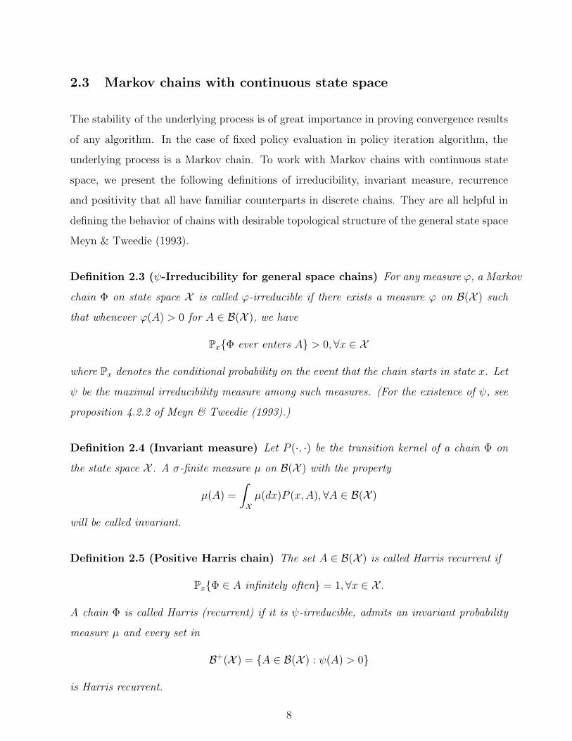
2.3 Markov chains with continuous state space

The stability of the underlying process is of great importance in proving convergence results

of any algorithm. In the case of fixed policy evaluation in policy iteration algorithm, the

underlying process is a Markov chain. To work with Markov chains with continuous state

space, we present the following definitions of irreducibility, invariant measure, recurrence

and positivity that all have familiar counterparts in discrete chains. They are all helpful in

defining the behavior of chains with desirable topological structure of the general state space

Meyn & Tweedie (1993).

Definition 2.3 (ψ-Irreducibility for general space chains) For any measure ϕ, a Markov

chain Φ on state space X is called ϕ-irreducible if there exists a measure ϕ on B(X ) such

that whenever ϕ(A) > 0 for A ∈ B(X ), we have

Px{Φ ever enters A} > 0,∀x ∈ X

where Px denotes the conditional probability on the event that the chain starts in state x. Let

ψ be the maximal irreducibility measure among such measures. (For the existence of ψ, see

proposition 4.2.2 of Meyn & Tweedie (1993).)

Definition 2.4 (Invariant measure) Let P (·, ·) be the transition kernel of a chain Φ on

the state space X . A σ-finite measure µ on B(X ) with the property

µ(A) =

∫Xµ(dx)P (x,A),∀A ∈ B(X )

will be called invariant.

Definition 2.5 (Positive Harris chain) The set A ∈ B(X ) is called Harris recurrent if

Px{Φ ∈ A infinitely often} = 1,∀x ∈ X .

A chain Φ is called Harris (recurrent) if it is ψ-irreducible, admits an invariant probability

measure µ and every set in

B+(X ) = {A ∈ B(X ) : ψ(A) > 0}

is Harris recurrent.

8

The most desired feature of a positive Harris chain is the applicability of the well-known

strong law of large numbers, which is summarized in the following lemma from Meyn &

Tweedie (1993). It is fundamental and essential to convergence analysis of different rein-

forcement learning and dynamic programming algorithms (parametric or non-parametric).

Lemma 2.1 (Law of large numbers for positive Harris chains) If Φ is a positive Har-

ris chain (see definition 2.5) with invariant probability measure µ, for each f ∈ L1(X ,B(X ), µ),

limn→∞

1

n+ 1

n∑i=0

f(xi) =

∫Xµ(dx)f(x)

almost surely.

2.4 Policy iteration

The main focus of the paper is policy iteration algorithms, which typically consist of two

loops: the inner loop for fixed policy evaluation and the outer loop for policy improvement.

The convergence of exact policy iteration for general state space is well known (see Bertsekas

& Shreve (1978)). The primary convergence result that is derived from the aforementioned

monotonicity and contraction properties of the Bellman’s operators M and Mπ is stated as

follows.

Proposition 2.1 Let (πn)∞n=0 be a sequence of policies generated recursively as follows: given

an initial policy π0, for n ≥ 0,

πn+1(x) = arg maxu{C(x, u) + γ

∫WQ(x, u, dw)V πn(SM(x, u, w))}.

Then V πn → V ∗ uniformly where V ∗ is the optimal value function.

However, the exact policy iteration algorithm is only conceptual because in practice the

expectation cannot be computed exactly. Hence, the approximate policy iteration algorithm,

in which the policy evaluation stops in finite time, is considered. In approximate policy

iteration, the estimated value function of a policy is random (a statistical estimate of the

true value function of the policy) because it depends on the sample trajectory of the chain

9

by following the policy and also the iteration counter of policy evaluation. Given the state

space being compact and the norm being the sup norm || · ||∞ for continuous functions, Ma

& Powell (2010) proves convergence in mean of the approximate policy iteration algorithm,

which is summarized in the following theorem.

Theorem 2.1 (Mean convergence of approximate policy iteration)

Let π0, π1, . . . , πn be the sequence of policies generated by an approximate policy iteration al-

gorithm and let V π0 , V π1 , . . . , V πn be the corresponding approximate value functions. Further

assume that, for each fixed policy πn, the MDP is reduced to a Markov chain that admits an

invariant probability measure µπn. Let {εn} and {δn} be positive scalars that bound the mean

errors in approximations to value functions and policies (over all iterations) respectively,

that is ∀n ∈ N,

Eµπn ||V πn − V πn||∞ ≤ εn, (12)

and

Eµπn ||Mπn+1Vπn −MV πn||∞ ≤ δn. (13)

Suppose the sequences {εn} and {δn} converge to 0 and

limn→∞

n−1∑i=0

γn−1−iεi =n−1

limi=0

γn−1−iδi = 0,

e.g. εi = δi = γi. Then, this sequence eventually produces policies whose performance

converges to the optimal performance in the mean:

limn→∞

Eµπn ||V πn − V ∗||∞ = 0.

In plain English, the above theorem states that the mean difference between the optimal

policy value function and the estimated policy value function using approximate policy it-

eration shrinks to 0 as the successive approximations of the value functions improve. This

result lays down the basic foundations for analyzing convergence properties of algorithms

using different kernel smoothing techniques that are discussed in later sections.

10

3 Least Squares Policy Iteration with Mercer Kernel

Temporal-difference (TD) learning algorithms (see Tsitsiklis & Van Roy (1997), Tadic (2001))

have been widely used for value function approximation in reinforcement learning, and least

squares temporal difference (LSTD) learning algorithms (Bradtke & Barto (1996), Boyan

(1999)) uses linear approximation and applies least squares method to improve data ef-

ficiency. Although LSTD learning has the merits of faster convergence rate and better

performance than conventional TD algorithms, least squares approaches can not be applied

directly to TD algorithm with nonlinear function approximation such as neural networks and

it has been shown that TD algorithms with nonlinear approximation can actually diverge

(see Tsitsiklis & Van Roy (1997)). To implement efficient and convergent TD learning with

nonlinear function approximation, in this section we study the temporal difference learning

algorithm that uses Mercer kernel functions to approximate value functions. Even though

the value function approximation with Mercer kernels is nonlinear and nonparametric, the

learning algorithms and the proof techniques for convergence analysis are all closely related

to the recursive least squares policy iteration algorithm with linear function approximation

owing to the famous kernel trick.

The trick known as Mercer’s theorem basically states that any continuous, symmetric

and positive semi-definite kernel function K(x, y) can be expressed as a dot product in a

high-dimensional feature space F .

Theorem 3.1 (Mercer’s theorem) Let S a measurable space and the kernel K be a pos-

itive and semi-definite function i.e.

∑i,j

K(si, sj)rirj ≥ 0

for any finite subset {s1, ..., sn} of S and any real numbers {r1, ..., rn}. There exists a function

φ : S → F , where F (feature space) is an inner product space of possibly high dimension,

such that

K(x, y) = 〈φ(x), φ(y)〉.

11

To solve non-linear problems, the kernel trick can be applied to map the original non-

linear space into a higher-dimensional inner product feature space F such that a linear

algorithm such as least squares can be subsequently used. As a result, the kernel trick

transforms a nonlinear algorithm to an equivalent linear one that operates on the feature

space F . This is only used to prove convergence of the algorithm. In the implementation of

the algorithm, the kernel function is used to replace any dot product between two vectors of

feature function φ. Hence, the inner products in feature space F do not make direct reference

to feature vectors and as a result the feature vectors are never explicitly calculated. This is

a desirable property for infinite-dimensional feature spaces such as the one associated with

Gaussian kernels where direct computation of the inner products is not feasible.

Moreover, the kernel function K determines a Hilbert space HK , which is often called

reproducing kernel Hilbert space (RKHS). HK is a vector space containing all linear combi-

nations of the functions K(·, x), f(·) =∑m

i=1 αiK(·, xi). Let g(·) =∑n

j=1 βjK(·, yj). Then

the inner product is defined as:

〈f, g〉 =m∑i=1

n∑j=1

αiβjK(xi, yj),

and the norm is defined as ||f ||HK =√〈f, f〉.

The Hilbert space L2 is usually too big for analysis purposes because it contains too many

non-smooth functions, while a RKHS is a restricted smooth function space smaller than the

general Hilbert space. To do convergence analysis, we impose the following assumption on

the policy value functions and the policy space Π.

Assumption 3.1 Assume that the policy value function for any fixed policy π ∈ Π is in the

RKHS HK.

Xu et al. (2007) proposes a kernel version of the least squares policy iteration (LSPI

see Lagoudakis & Parr (2003)) algorithm, which applies the kernel recursive least squares

algorithm developed in Engel et al. (2004) to the LSTD-Q algorithm for approximating

station-action Q-factor of a fixed policy. The algorithm is empirically shown to provide better

12

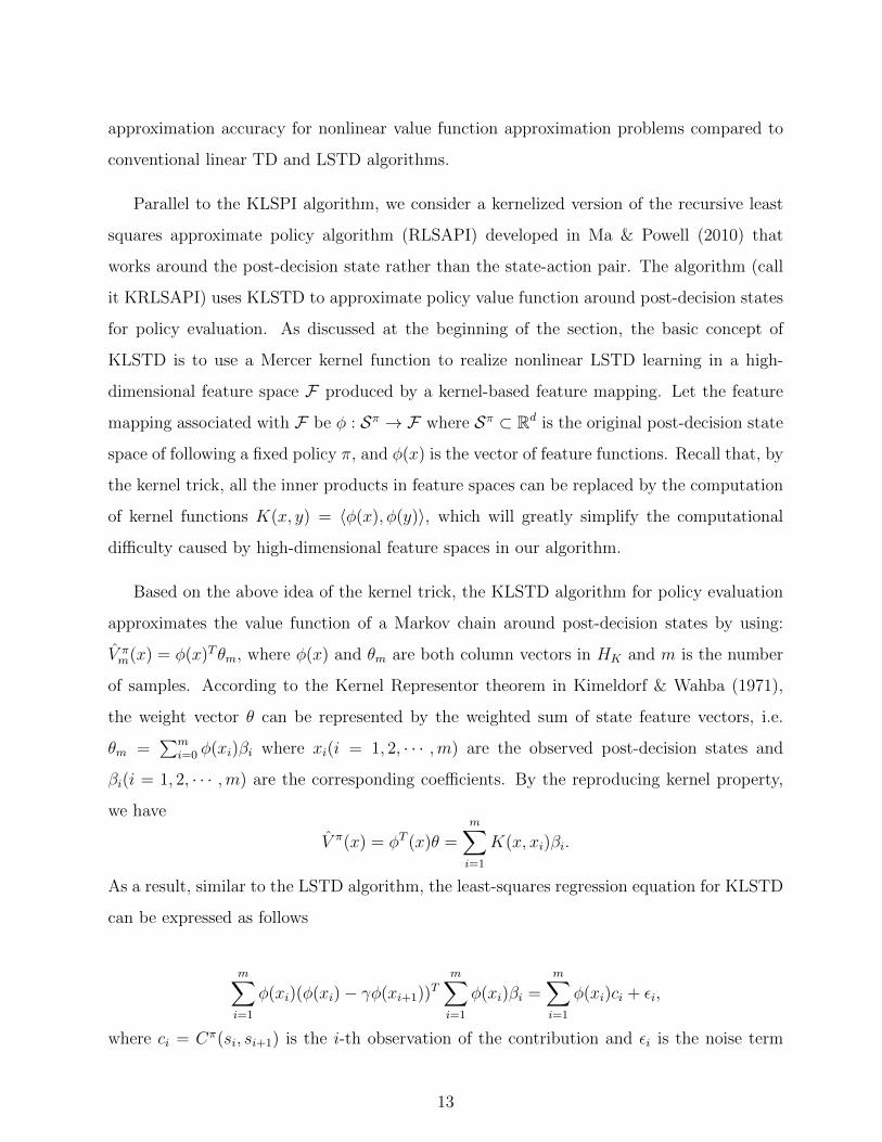
approximation accuracy for nonlinear value function approximation problems compared to

conventional linear TD and LSTD algorithms.

Parallel to the KLSPI algorithm, we consider a kernelized version of the recursive least

squares approximate policy algorithm (RLSAPI) developed in Ma & Powell (2010) that

works around the post-decision state rather than the state-action pair. The algorithm (call

it KRLSAPI) uses KLSTD to approximate policy value function around post-decision states

for policy evaluation. As discussed at the beginning of the section, the basic concept of

KLSTD is to use a Mercer kernel function to realize nonlinear LSTD learning in a high-

dimensional feature space F produced by a kernel-based feature mapping. Let the feature

mapping associated with F be φ : Sπ → F where Sπ ⊂ Rd is the original post-decision state

space of following a fixed policy π, and φ(x) is the vector of feature functions. Recall that, by

the kernel trick, all the inner products in feature spaces can be replaced by the computation

of kernel functions K(x, y) = 〈φ(x), φ(y)〉, which will greatly simplify the computational

difficulty caused by high-dimensional feature spaces in our algorithm.

Based on the above idea of the kernel trick, the KLSTD algorithm for policy evaluation

approximates the value function of a Markov chain around post-decision states by using:

V πm(x) = φ(x)T θm, where φ(x) and θm are both column vectors in HK and m is the number

of samples. According to the Kernel Representor theorem in Kimeldorf & Wahba (1971),

the weight vector θ can be represented by the weighted sum of state feature vectors, i.e.

θm =∑m

i=0 φ(xi)βi where xi(i = 1, 2, · · · ,m) are the observed post-decision states and

βi(i = 1, 2, · · · ,m) are the corresponding coefficients. By the reproducing kernel property,

we have

V π(x) = φT (x)θ =m∑i=1

K(x, xi)βi.

As a result, similar to the LSTD algorithm, the least-squares regression equation for KLSTD

can be expressed as follows

m∑i=1

φ(xi)(φ(xi)− γφ(xi+1))Tm∑i=1

φ(xi)βi =m∑i=1

φ(xi)ci + εi,

where ci = Cπ(si, si+1) is the i-th observation of the contribution and εi is the noise term

13

for each time step.

The single-step regression function is

φ(si)(φ(si)− γφ(si+1))Tm∑i=1

φ(si)βi =m∑i=1

φ(si)ci + εi.

Let Φm = [φ(x1), · · · , φ(xm)]T and km(xi) = [K(x1, xi), · · · , K(xm, xi)]T . By multiplying Φm

on both sides of the previous equation, due to the kernel trick, we have

km(xi)(km(xi)− γkm(xi+1))βm = km(xi)ci + Φmεi.

Then the new least squares regression function is

m∑i=1

km(xi)(km(xi)− γkm(xi+1))βm =m∑i=1

km(xi)ci.

Let Mm =∑m

i=1 km(xi)(km(xi) − γkm(xi+1)) and bm =∑m

i=1 km(xi)ci. Then, the recursive

least squares solution to the kernel-based TD learning problem is βm = M−1m bm with

Mm+1 = Mm + km+1(xm+1)(kTm+1(xm+1)− γkTm+1(xm+2))

and

bm+1 = bm + km+1(xm+1)cm.

Similar to the KLSPI in Xu et al. (2007), KRLSAPI uses KLSTD for policy evaluation

and makes policy improvement until the optimal policy is reached. In KLSPI or KRLSAPI,

the kernel-based feature vectors are automatically generated by the kernel function. This

data-driven automatic feature selection provides an efficient solution to the fundamental

difficulty of the LSPI algorithm. The details of the KLSPI algorithm is shown in figure 1. It

is worth noting that the arg max function in step 7 is usually a multivariate and potentially

non-convex optimization problem, which may require an external solver such as a nonlinear

proximal point algorithm (Luque (1987)).

Moreover, the approximation and generalization ability of kernel methods greatly con-

tribute to the convergence and performance of the approximate policy iteration algorithm.

We start with the convergence analysis of the policy evaluation. The following theorem

presents that the KLSTD algorithm converges in probability.

14

Figure 1: Kernel-based Recursive Least Squares Approximate Policy Iteration (KRLSAPI)

Step 0: Initialization:

Step 0a. Set the initial policy π0.

Step 0b. Set the kernel function K.

Step 0c. Set the iteration counter n = 0.

Step 0d. Set the initial State S00 .

Step 1: Do for n = 0, . . . , N ,

Step 2: Do for m = 1, . . . ,M :

Step 3: Initialize cm = 0.

Step 4: Choose one step sample realization ω.

Step 5: Do the following:

Step 5a. Set xnm = πn.

Step 5b. Compute Sn,xm = SM,x(Snm, xnm) and Snm+1 = SM(Sn,xm ,Wm+1(ω)).

Step 5c. Compute and store the corresponding kernel function valuekm(Sn,xm ) and km(Sn,xm+1) in dictionary.

Step 6: Do the following:

Step 6a. Compute and store cm = C(Snm, xnm) and Mm and bm

Step 6b. Update parameters βn,m = M−1m bm

Step 7: Update the parameter and the policy:

βn+1 = βn,M ,

πn+1(s) = arg maxx∈X{C(s, x) + γkTsx β

n+1}.

Step 8: Return the policy πNt and parameters βN .

Theorem 3.2 (Convergence of KLSTD in probability) Suppose assumptions 2.1 and

2.2 hold and the Markov chain of the post-decision states (following a fixed policy π) follows

a positive Harris chain having transition kernel P (x, dy) and invariant probability measure

µ. Further assume the policy value function V π is in the reproducing kernel Hilbert space

HK with the kernel function K being C∞ and ||K||∞ ≤ M for some constant M . Then,

V πm → V π in probability where V π

m(x) =∑m

i=1K(x, xi)βi.

15

We provide a sketch of the proof and omit details. We know that

V πm(x) = arg min

f∈HK{Remp(f) + λ||f ||HK}

where Remp is the empirical quadratic loss function and λ ≥ 0 is the regularization term (in

the original version of KLSTD, λ = 0). By the proof to corollary 6.2 of Wu et al. (2006) and

theorem 6 of Smale & Zhou (2005), for any 0 < ε < 1 we have with probability 1− ε

||V πm − V π||HK ≤ C(

log(4/ε)2

m)16

where C is a constant. Therefore, V πm → V π in HK norm in probability. By the reproducing

property of the kernel and the Cauchy-Schwartz inequality, we have for any x,

f(x)2 = 〈K(·, x), f〉2 ≤ K(x, x)||f ||2HK .

As a result,

||V πm − V π||∞ ≤

√M ||V π

m − V π||HK .

Hence, ||V πm → V π||∞ → 0 in probability. Moreover, we have Eµπ ||V π

m → V π||∞ → 0 since

V πm → V π are uniformly bounded owing to bounded kernel and compact post-decision space.

The convergence of KRLSAPI is fully determined by the convergence of the KLSTD

algorithm and the approximate errors of the policy evaluation and policy updating in the

approximate policy iteration algorithm. The following theorem illustrates the details. The

proof is omitted since it is a direct application of theorems 3.2 and 2.1.

Corollary 3.1 (Mean convergence of KRLSAPI) Suppose assumptions in theorem3.2

and assumption 3.1 hold. Theorem 2.1 applies to the kernel least squares approximate policy

iteration algorithm in figure 1.

To make the aforementioned Kernel algorithm practical, one key problem is to decrease

the computational and memory costs of kernel vectors, whose dimension is originally equal

16

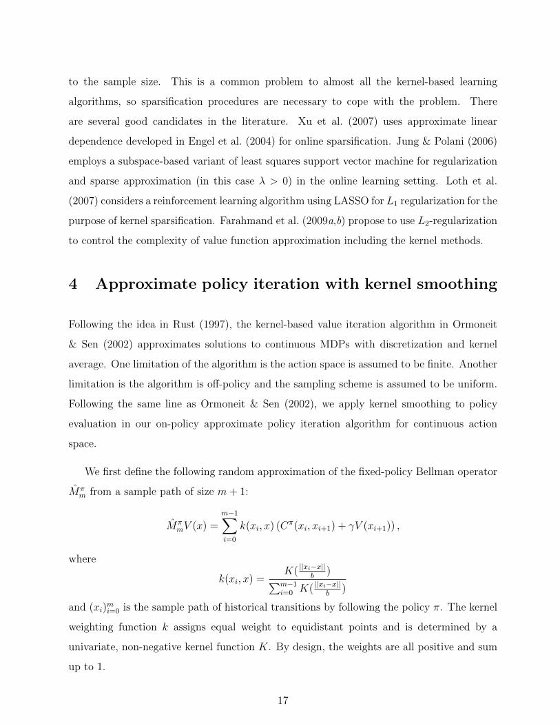
to the sample size. This is a common problem to almost all the kernel-based learning

algorithms, so sparsification procedures are necessary to cope with the problem. There

are several good candidates in the literature. Xu et al. (2007) uses approximate linear

dependence developed in Engel et al. (2004) for online sparsification. Jung & Polani (2006)

employs a subspace-based variant of least squares support vector machine for regularization

and sparse approximation (in this case λ > 0) in the online learning setting. Loth et al.

(2007) considers a reinforcement learning algorithm using LASSO for L1 regularization for the

purpose of kernel sparsification. Farahmand et al. (2009a,b) propose to use L2-regularization

to control the complexity of value function approximation including the kernel methods.

4 Approximate policy iteration with kernel smoothing

Following the idea in Rust (1997), the kernel-based value iteration algorithm in Ormoneit

& Sen (2002) approximates solutions to continuous MDPs with discretization and kernel

average. One limitation of the algorithm is the action space is assumed to be finite. Another

limitation is the algorithm is off-policy and the sampling scheme is assumed to be uniform.

Following the same line as Ormoneit & Sen (2002), we apply kernel smoothing to policy

evaluation in our on-policy approximate policy iteration algorithm for continuous action

space.

We first define the following random approximation of the fixed-policy Bellman operator

Mπm from a sample path of size m+ 1:

MπmV (x) =

m−1∑i=0

k(xi, x) (Cπ(xi, xi+1) + γV (xi+1)) ,

where

k(xi, x) =K( ||xi−x||

b)∑m−1

i=0 K( ||xi−x||b

)

and (xi)mi=0 is the sample path of historical transitions by following the policy π. The kernel

weighting function k assigns equal weight to equidistant points and is determined by a

univariate, non-negative kernel function K. By design, the weights are all positive and sum

up to 1.

17

Since we have the fixed point property V π = MπV π for Mπ, MπmV

π could be viewed

as an approximation of V π. First, we use the random operator Mπ to estimate the true

post-decision policy value function V π on the finite sample of post-decision states (xi)mi=1 by

finding the fixed point solution the approximate Bellman equation

V π = MπmV

π = P π[cπ + γV π], (14)

where V π is a vector of m for post-decision decision states (xi)mi=1, P π is a m×m stochastic

matrix with i, j-th entry being k(xi−1, xj) for i, j ∈ {1 · · ·m} and cπ is the reward vector of

dimension m with i-th entry being Cπ(xi−1, xi) for i ∈ {1 · · ·m}. Since P π is a stochastic

matrix, I−γP π is nonsingular. This guarantees the existence and uniqueness of the solution,

which is simply

V π = (I − γP π)−1cπ. (15)

Then, the algorithm extrapolates the policy value function estimate to x ∈ X π \{xi}mi=1 with

V π(x) =m−1∑i=0

k(xi, x)(Cπ(xi, xi+1) + γV π(xi+1)

). (16)

Figure 2 illustrates details of the kernel-based approximate policy iteration algorithm.

In order to show convergence of the algorithm, we first introduce the following addi-

tional technical assumption on state space, contribution function, kernel function and the

underlying Markov chain.

Assumption 4.1

a. For each policy π ∈ Π, Sπ = [0, 1]d.

b. The contribution function, Cπ(x, y) is a jointly Lipschitz continuous function of x and y

i.e. there exists a KC > 0 such that

|r(x′, y′)− r(x, y)| ≤ KC ||(x′ − x, y′ − y)||. (17)

18

Figure 2: Approximate policy iteration with kernel smoothing (KSAPI)

Step 0: Initialization:

Step 0a. Set the initial policy π0.

Step 0b. Set the kernel function K.

Step 0c. Set the iteration counter n = 0.

Step 1: Do for n = 0, . . . , N ,

Step 1a. Set the iteration counter l = 0.

Step 1b. Set the initial state xn0 .

Step 1c: Do for j = 0, · · · ,m:

Step 1c.1: Set unj = πn(xnj ) and draw randomly or observe Wj+1 from thestochastic process,

Step 1c.2: Compute xn,πj = SM,π(xnj , unj ) (store also) and xnj+1 =

SM(xn,πj , unj ,Wj+1).

Step 1d. Let cπ be a vector of dimensionality m with i-th entry Cπ(xn,πi−1, xn,πi ) for

i = 1 · · ·m.

Step 1e. Let P π be a matrix of dimensionality m×m with i, j-th entry k(xn,πi−1, xn,πj )

for i, j ∈ {1 · · ·m}.

Step 2: Solve for v = (I − γP π)−1cπ with v being a vector of dimensionality m withi-th element v(xn,πi ) for i = 1 · · ·m.

Step 3: Let vn(x) =∑m−1

i=0 k(xn,πi , x)(Cπ(xn,πi , xn,πi+1) + γv(xn,πi+1)

)Step 4: Update the policy:

πn+1(x) = arg maxu∈U{C(x, u) + γvn(xu)}.

Step 5: Return the policy πN+1.

c. The kernel function K+ : [0, 1] → R+ is Lipschitz continuous, satisfying∫ 1

0K+(x)dx = 1

and K is the completion of K+ on R.

d. For each policy π ∈ Π, the invariant probability measure µπ is absolutely continuous with

respect to the Lebesgue measure λ and 0 < Kπ ≤ dµπdλ≤ Kπ. In other words, the invariant

probability measure µπ has a continuous density function fπ such that fπ is bounded from

19

above and away from 0 on Sπ.

Remark: It looks like we place a strong restriction on the post-decision state space to a

d-dimensional unit cube [0, 1]d in part a of assumption 4.1. However, the assumption can be

relaxed to the state space X π = [a1, b1] × · · · × [ad, bd]. We know that X π is isomorphic to

[0, 1]d with a bijective linear mapping L : X π → [0, 1]d. Let P π, µπ and V π be the transition

kernel, invariant measure and policy value function on X π. Then, P π ◦ L−1, µπ ◦ L−1 and

V π ◦L−1 are the corresponding counterparts for [0, 1]d. Hence, we can assume the state space

is [0, 1]d without loss of generality since we can recover the policy value function V π on X π

from V π ◦ L−1 on [0, 1]d using the identity V π = V π ◦ L−1 ◦ L.

We first present the following lemma on kernel volume bound, which provides crucial

bounds in the main convergence result.

Lemma 4.1 (Kernel volume bound) Let Kv =∫

[0,1]dK( ||u−y||

b)µπ(du) and νn =

∫ 1

0rnK(r)dr.

Kv ≥ bd2πd/2νd−1Kπ

Γ(d/2)where Γ(·) is Euler’s gamma function.

Proof:

By assumption 4.1.d,

∫[0,1]d

K(||u− y||

b)µπ(du) =

∫[0,1]d

K(||u− yb||)fπ(u)du

≥ Kπ

∫[0,1]d

K(||u− yb||)du

= Kπbd

∫Rd

K(||u||)du

=bd2πd/2Kπ

Γ(d/2)

∫ 1

0

rd−1K(r)dr.

We now present the convergence in mean of the policy evaluation step in figure 2.

20

Theorem 4.1 (Convergence in the mean of policy evaluation) Suppose assumptions

2.1, 2.2 and 4.1 hold and the Markov chain of the post-decision states follows a positive Har-

ris chain having transition kernel P (x, dy) and invariant probability measure µ. Let the

bandwidth b(m) satisfy b(m)d+1√m → ∞ and b(m) → 0 e.g. b(m) = m−

12(d+2) . Let V π

m be

defined as in (16). Then Eµπ ||V πm − V π||∞ → 0 as m→∞.

Proof:

First define the asymptotic weighting kernel function k be:

k(x, y) =K( ||x−y||

b)∫

[0,1]dK( ||u−y||

bµπ(du)

. (18)

Since the chain is positive Harris, by lemma 2.1

mk(x, y) =K( ||x−y||

b)

1m

∑m−1i=0 K( ||Xi−y||

b)→ k(x, y) (19)

almost surely as m→∞. For any Lipschitz continuous V ∈ C([0, 1]d), define

MπV (x) = k(X, x)(Cπ(X, Y ) + γV (Y )), (20)

and we can write

MπmV (x) = MmV (x) =

m−1∑i=0

k(Xi, x)∑m−1i=0 k(Xi, x)

(Cπ(Xi, Xi+1) + γV (Xi+1)), (21)

since k is the kernel function K normalized by∫

[0,1]dK(||u−y||b

)µπ(du). Then, we have

almost surely

limm→∞

MπmV (x) = lim

m→∞

1

m

m−1∑i=0

K( ||xi−x||b

)1m

∑m−1i=0 K( ||xi−x||

b)

(Cπ(xi, xi+1) + γV (xi+1))

=

∫[0,1]d

∫[0,1]d

K( ||z−x||b

)∫[0,1]d

K( ||u−x||b

)µπ(du)(Cπ(z, w) + γV (w))P π(z, dw)µπ(dz)

=

∫[0,1]d

∫[0,1]d

k(z, x) (Cπ(z, w) + γV (w))P π(z, dw)µπ(dz)

= EµπMπV (x).

21

Since MπmV are uniformly bounded, we have

EµπMπmV → EµπMπV (x). (22)

By the triangle inequality, we have

||MπmV −MπV ||∞ ≤ ||Mπ

mV − EµπMπV )||∞ + ||EµπMπV −MπV ||∞.

We note that the first term ||MπmV − EµπMπV ||∞ is random and the second term

||EµπMπV −MπV ||∞ is deterministic. Therefore, it suffices to show the first term converges

to 0 in the mean and the last term converges to 0 separately.

Define

MπmV (x) =

m−1∑i=0

k(Xi, x)

m(Cπ(Xi, Xi+1) + γV (Xi+1)). (23)

Again it is easy to see that MπmV (x)→ EµπMπV (x) almost surely. In turn, EµπMπ

mV (x)→

EµπMπV (x) pointwise. Since EµπMπmV (x) has uniform Lipschitz continuous constant, the

sequence is equicontinuous. As a result, we have EµπMπmV → EµπMπV uniformly. We write

||MπmV − EµπMπV ||∞ ≤ ||Mπ

mV − MπmV ||∞ + ||Mπ

mV − EµπMπmV ||∞

+||EµπMπmV − EµπMπV ||∞.

Note ||EµπMπmV − EµπMπV ||∞ is deterministic and ||EµπMπ

mV − EµπMπV ||∞ → 0.

By following a similar argument as in lemma 1 of Ormoneit & Sen (2002), we have for any

fixed bandwidth b > 0, the sequence√m(Mπ

mV (x)−EµπMπmV (x)]) converges in distribution

to a Gaussian process on C([b, 1− b]d). Then, by theorem 3.2 of Rust (1997),

Eµπ√m||Mπ

mV − Eµπ(MπmV )||∞ ≤

√π

2(1 + d

√πC)Kk||C

π + γV ||∞, (24)

22

where C is a constant and Kk is the Lipschitz constant of k.

For fixed y, by lemma 4.1 we have

|k(x, y)− k(x′, y)| =1∫

[0,1]dK( ||u−y||

b)µπ(du)

|K(||x− y||

b)−K(

||x′ − y||b

)|

≤ Γ(d/2)Kk

bd2πd/2νd−1Kπ

| ||x− y||b

− ||x′ − y||b

|

≤ Γ(d/2)Kk

bd+12πd/2νd−1Kπ

||x− x′||.

Hence, we have

Eµπ ||MπmV − Eµπ(Mπ

mV )||∞ ≤(1 + d

√πC)Γ(d/2)Kk

bd+1√m2√

2π(d−1)/2νd−1Kπ

||Cπ + γV ||∞.

We write

|MπmV (x)− Mπ

mV (x)| = |MπmV (x)− Mπ

mV (x)|

=m−1∑i=0

k(Xi, x)∑m−1i=0 k(Xi, x)

(Cπ(Xi, Xi+1) + γV (Xi+1))(1− 1

m

m−1∑i=0

k(xi, x))

Hence, by the proof of corollary to theorem 3.4 in Rust (1997),

||MπmV − Mπ

mV ||∞ ≤ ||Cπ + γV ||∞ supx∈[0,1]d

|1− 1

m

m−1∑i=0

k(xi, x)|,

and

Eµπ supx∈[0,1]d

|1− 1

m

m−1∑i=0

k(xi, x)| ≤ C ′Kk√m≤ C ′Γ(d/2)Kk

bd+1√m2πd/2νd−1Kπ

,

where C ′ is a constant. Therefore,

Eµπ ||MπmV − EµπMπV ||∞ → 0

23

as bd+1√m→∞.

Let h(x) = MπV (x) =∫

[0,1]dP π(x, dy)(Cπ(x, y) + γV (y)) and Kh be the Lipschitz con-

stant of h. Then,

||EµπMπV −MπV ||∞ = supx∈[0,1]d

∣∣∣∣∫[0,1]d

k(u, x)(h(u)− h(x))µπ(du)

∣∣∣∣≤ sup

x∈[0,1]d

∫[0,1]d

k(u, x)|h(u)− h(x)|µπ(du)

≤ supx∈[0,1]d

KhKπ

Γ(d/2)

bd2πd/2νd−1

Kπ

∫[0,1]d

K(||u− x||

b)||u− x||du

≤ KhKπ

Γ(d/2)bd+1

bd2πd/2νd−1

Kπ

∫Rd

K(||u||)||u||du

≤ KhKπ

Γ(d/2)b

2πd/2νd−1

Kπ

∫ 1

0

rd−1K(r)rdr

≤ bKhKπνd

Kπνd−1

.

Hence, ||EµπMπV −MπV ||∞ → 0 as b(m)→ 0.

Since it is easy to check that Mπm defines a contraction and let V π

m = MπmV

πm (as defined

in (16)), then

||V πm − V π||∞ ≤ ||Mπ

mVπm − Mπ

mVπ||∞ + ||Mπ

mVπ − V π||∞

≤ γ||V πm − V π||∞ + ||Mπ

mVπ −MπV π||∞.

Hence, we have

Eµπ ||V πm − V π||∞ ≤

1

1− γEµπ ||Mπ

mVπ −MπV π||∞. (25)

This implies that Eµπ ||V πm − V π||∞ → 0.

Corollary 4.1 (Convergence in the mean of kernel-based API) Suppose assumptions

24

in theorem 4.1 hold for all policies π ∈ Π. Theorem 2.1 applies to the kernel-based approxi-

mate algorithm in figure 2.

The proof is omitted since it is a direct application of theorems 4.1 and 2.1. It is worth

noting that the matrix inversion in step 2 of the algorithm in figure 2 demands O(m3)

computational complexity, which can be burdensome for large m. Hence, we consider a value

iteration type updating rule (O(m2) computational complexity) for policy value function

estimates, which can be written compactly using matrix notation:

V πm,k+1 = P π(Cπ + γV π

m,k) (26)

where V πm,k and V π

m,k+1 are the old and new policy value function estimates respectively.

Since the random operator Mπ is a contraction operator, by the Banach fixed point theorem

the updating in (26) converges to a unique fixed point that satisfies equation (14), which is

V πm. The algorithm in figure 3 that uses the updating in equation (26) is a type of hybrid

value/policy iteration algorithm.

We now analyze the convergence of the hybrid algorithm.

Corollary 4.2 (Convergence in the mean of the hybrid kernel-based hybrid API)

Suppose assumptions in theorem 4.1 hold for all policies π ∈ Π. Theorem 2.1 applies to the

hybrid kernel-based approximate algorithm in figure 3 with policy evaluation stopping crite-

rion that satisfies

||V πm,k+1 − V π

m,k||∞ ≤1− γ

2γεn. (27)

Proof:

In each inner loop, first determine m such that Eµπ ||V πm−V π||∞ ≤ εn

2. Since we have almost

surely

supx∈{xi}m−1

i=0

|V πm,k(x)− V π

m(x)| → 0,

25

Figure 3: Hybrid value/policy iteration with kernel smoothing (KSHPI)

Step 0: Initialization:

Step 0a. Set the initial policy π0.

Step 0b. Set the kernel function K.

Step 0c. Set the iteration counter n = 0.

Step 1: Do for n = 0, . . . , N ,

Step 1a. Set the iteration counter l = 0.

Step 1b. Set the initial state xn0 .

Step 1c: Do for j = 0, · · · ,m:

Step 1c.1: Set unj = πn(xnj ) and draw randomly or observe Wj+1 from thestochastic process,

Step 1c.2: Compute xn,πj = SM,π(xnj , unj ) (store also) and xnj+1 =

SM(xn,πj , unj ,Wj+1).

Step 1d. Initialize v0 where v0 is a vector of dimensionality m with element v0(xn,pii )for i = 1 · · ·m.

Step 1e. Let Cπ be a vector of dimensionality m with i-th entry Cπ(xn,πi−1, xn,πi ) for

i = 1 · · ·m.

Step 1f. Let P π be a matrix of dimensionality m×m with i, j-th entry k(xn,πi−1, xn,πj )

for i, j ∈ {1 · · ·m}.

Step 2: Do for l = 0, . . . , L− 1:

Step 2.1: vl+1 = cπ + γP πvl.

Step 3: Let vn(x) =∑m−1

i=0 k(xn,πi , x)(Cπ(xn,πi , xn,πi+1) + γvL(xn,πi+1)

)Step 4: Update the policy:

πn+1(x) = arg maxu∈U{C(x, u) + γvn(xu)}.

Step 5: Return the policy πN+1.

||V πm,k − V π

m||∞ → 0 almost surely. With the stopping criterion (27), we have almost surely,

||V πm,K+1 − V π

m||∞ ≤1

1− γ||V π

m,K+1 − V πm,K ||∞ ≤

εn2.

Taking expectations, we obtain Eµπ ||V πm,k+1 − V π||∞ ≤ εn. Hence, theorem 2.1 applies.

26

5 Finite horizon approximation using recursive kernel

smoothing and local polynomials

In this section, we propose an algorithm that applies kernel smoothing to finite horizon

rewards to approximate policy value function for the infinite horizon problems. The logic

behind this idea is very simple. We approximate the infinite horizon post-decision policy

value function V π with its k-th finite horizon policy value function

V πk (x) = E

{k∑t=0

γtCπ(xt, xt+1)|x0 = x

}. (28)

It is worth noting that x’s are all post-decision states. Let Cmax be the constant that bounds

the contribution function Cπ and ε > 0. There exists k ∈ N such that for all x ∈ X π,

|V πk (x)− V π(x)| =

∣∣∣∣∣E{

∞∑t=k+1

γtCπ(xt, xt+1)|x0 = x

}∣∣∣∣∣ ≤ γk+1

1− γCmax < ε.

As a result, for each fixed policy π we can approximate the post-decision policy value

function arbitrarily well with a finite horizon policy value function. Hence, we can apply ker-

nel regression techniques such as Nadaraya-Watson estimate and local polynomial regression

(recursive or non-recursive) to estimate the finite horizon policy value function with data

(xi, yi) where

yi =i+k∑t=i

γt−iCπ(xt, xt+1). (29)

The details of the kernel smoothing approximate policy iteration algorithm with finite horizon

approximation are shown in figure 4.

In order to apply theorem 2.1 to show the convergence of the algorithm, it suffices to

use the kernel regression estimation techniques that satisfy strong uniform convergence to

the finite horizon policy value function. We consider the following generic form of the kernel

smoothing estimate

m(x) =1

nhd

n∑i=1

YiK(x−Xi

h) (30)

27

Figure 4: Approximate policy iteration with kernel smoothing and finite horizon rewards(KSFHRAPI)

Step 0: Initialization:

Step 0.1: Set the initial policy π0 and the iteration counter n = 0.

Step 0.2: Set the kernel function K and fixed horizon number k ≥ 1.

Step 1: Do for n = 0, . . . , N ,

Step 1.1: Set the iteration counter m = 0 and the initial state xn0 .

Step 2: Do for m = 0, . . . ,M :

Step 2.1: If m = 0, do the following:

Step 2.1.1: Set the initial state xn0 , initial kernel estimate fn−1 = 0 andvm = 0

Step 2.1.2: Draw randomly or observe W1, · · · ,Wk+1 from the stochasticprocess.

Step 2.1.3: Do for j = 0, · · · , k:

Step 2.1.3.a: Set unj = πn(xnj ).

Step 2.1.3.b: Compute xn,πj = SM,π(xnj , unj ) and xnj+1 =

SM(xn,πj , unj ,Wj+1).

Step 2.2: If m = 1, . . . ,M , do the following:

Step 2.2.1: Draw randomly or observe Wm+k+1 from the process.

Step 2.2.2 Set unm+k = πn(xnm+kn).

Step 2.2.3 Compute xn,πm+k = SM,π(xnm+k, unm+k) and

xnm+k+1 = SM(xnm+k, unm+k,Wm+k+1).

Step 2.2.4 Compute unm+k+1 = πn(xnm+k+1) and

xn,πm+k+1 = SM,π(xnm+k+1, unm+k+1).

Step 2.3: Compute vm =∑k−1

j=0 γjCπ(xn,πm+j, x

n,πm+j+1).

Step 2.4: Apply kernel methods with sparsification and compute kernel esti-mate fnm with (xn,πj )mj=0 and (vj)

mj=0

or recursively with fnm−1, xn,πm and vm.

Step 3: Update the policy:

πn+1(x) = arg maxu∈U{C(x, u) + γfnM(xu)}.

Step 4: Return the policy πN+1.

28

where h is a bandwidth and K : Rd → R is a kernel function. With proper choice of the

kernel function K, the generic form includes most kernel-based nonparametric estimators

such as kernel density estimators of density functions, Nadaraya-Watson estimators of the

regression function, and local polynomial estimators.

There are numerous strong uniform convergence results under various technical condi-

tions for the generic form of kernel regression estimates. The most common convergence

results can be found for the case when the data are sampled with identical and indepen-

dent distribution (e.g. Mack & Silverman (1982)). However, these results are less relevant

because dependence in data structure arises naturally in Markov decision process problems.

Peligrad (1992), Masry (1996), Fan & Yao (2003) provide strong uniform convergence results

under dependent data structure assumptions. Hansen (2008) generalizes previous results and

proves strong uniform convergence for kernel regression estimation under milder conditions

such as stationary strong mixing data with infinite support and kernels with unbounded

support. Therefore, to prove convergence of the policy iteration algorithm, we consider the

same set of assumptions and check whether they are satisfied in our setting of the problem

class.

The following assumption stipulates that the kernel function K is bounded, integrable

and smooth e.g. being Lipschitz continuous on a truncated support or having a bounded

derivative with an integrable tail. This assumption admits a lot of commonly used kernels,

such as the (higher order) polynomial kernels and the (higher order) Gaussian kernels (see

Hansen (2008)).

Assumption 5.1 (Kernel) Let K be a kernel function. |K(x)| ≤ K1 for all x and∫Rd |K(x)|dx ≤

K2 <∞. Furthermore suppose for some K3, C <∞, either |K(x)| = 0 for all |x| ≥ K3 and

∀x, x′ ∈ Rd

|K(x)−K(x′)| ≤ C||x− x′||,

or ∂∂xK(x) ≤ K3 and for some ν > 1, ∂

∂xK(x) ≤ K3||x||ν for ||x|| > C.

Before presenting the assumption on the chain, we first present the definition of strong

29

mixing (α mixing) condition.

Definition 5.1 (Strong (α) mixing) Let (Xt)∞t=0 be a sequence of random variables. The

strong mixing coefficient is defined as

α(n) = sup{|P(A ∩B)− P(A)P(B)| : k ≥ 0, A ∈ Fk, B ∈ F∞k+n}, (31)

where Fk = σ(X0, · · · , Xk) and F∞k+n = σ(Xk+n, · · · ). The process X is strong mixing if

α(n)→ 0 as n→∞.

The following assumption specifies the technical dependence structures of the data such

as stationarity and the strong mixing property with a certain decay rate. It also requires

boundedness of the marginal density function, joint density and conditional expectations of

Y .

Assumption 5.2 (Data structure)

a. The data sequence (Xn, Yn) is a strictly stationary and strong process mixing with

mixing coefficients α(n) that satisfy α(n) ≤ An−β where A < ∞ and for some s > 2

E|Y0|s <∞ and β > 2s−2s−2

.

b. Xn has marginal density f such that supx f(x) ≤ B1 <∞ supx E[|Y0|s|X0 = x]f(x) ≤

B2 <∞.

c. There is some j∗ < ∞ such that for all j > j∗ supx0,xj E[|Y0Yj||X0 = x0, Xj =

xj]fj(x0, xj) ≤ B3 <∞ where fj(x0, xj) denotes the joint density of X0, Xj.

Now we check if the above assumption on data structure is satisfied in our problem setting

of MDP. Suppose we initialize the chain according to its invariant measure µπ. Then the

data sequence is strictly stationary. The following lemma 5.1 exhibits that the data is strong

mixing.

30

Lemma 5.1 (Strong mixing of the data) The data in figure 4 for policy evaluation is a

strong mixing process given the post decision states for a fixed policy π evolves according to

a positive Harris chain.

Proof:

Let Zi = (Xi, Xi+1, · · · , Xi+k). Since X is a Markov chain, Z is a Markov chain with

transition kernel

PZ(z, A) =k∏i=1

1xi∈Ai−1PX(xk, Ak),

where z = (x0, x1, · · · , xk) and A = A0×A1 · · · ×Ak. Since X is positive Harris by assump-

tion, it has an invariant measure πX . We claim Z has an invariant measure

µZ(dz) = µX(dx0)PX(x0, dx1) · · ·PX(xk−1, dxk)

where z = (x0, · · · , xk). For simplicity of presentation, consider the case k = 1. Then we

have

µZ(A×B) =

∫A×B

µX(dx0)PX(x0, dx1) =

∫A

µX(dx0)PX(x0, B) (32)

and

∫µZ(dz)PZ(z, A×B) =

∫µX(dx0)PX(x0, dx1)1x1∈AP (x1, B)

=

∫µX(dx1)1x1∈AP (x1, B)

=

∫A

µX(dx1)PX(x1, B).

Hence, µZ is the invariant measure for Z. Consider ||(PZ)n(z, ·)−µZ(·)||TV where || · ||TV is

the total variation norm. We have

(PZ)n(z,k∏i=0

Ak) = P(Xn ∈ A0, · · · , Xn+k ∈ Ak|X0 = x0, · · · , Xk = xk)

= P(Xn ∈ A0, · · · , Xn+k ∈ Ak|Xk = xk)

31

where z = (x0, · · · , xk). Since (X) is positive Harris, as n→∞

||(PZ)n(z, ·)− µZ(·)||TV = sup∏ki=0 Ak

|P(Xn ∈ A0, · · · , Xn+k ∈ Ak|Xk = xk)

−∫A0×···Ak−1

µX(dx0)PX(x0, dx1) · · ·PX(xk−2, dxk−1)PX(xk−1, Ak)|

→ 0

for all xk ∈ X π. Therefore, Z is also positive Harris. As a result, by theorem A of Athreya

& Pantula (1986), Z is strong mixing, meaning αZ(n) → 0 as n → ∞. We also note that

there is a measurable function g :∏k

j=0X → X × R such that g(Zi) = (Xi, Yi). We claim

g(Z) is strong mixing. First, we note that Fg(Z) ⊂ FZ since g is measurable. Then,

αg(Z)(n) = sup{|P(A ∩B)− P(A)P(B)| : k ≥ 0, A ∈ Fg(Z)k , B ∈ (Fg(Z))∞k+n}

≤ sup{|P(A ∩B)− P(A)P(B)| : k ≥ 0, A ∈ FZk , B ∈ (FZ)∞k+n}

= αZ(n).

Since Yn’s are bounded in discounted problems, we can take s = ∞ and let β > 2. In

order to have uniform convergence, further restriction has to be put on β i.e. β > 1 + d+ dq

for some q > 0 (see Hansen (2008)). In addition, the boundedness condition on conditional

expectations are reduced to the boundedness of density and joint density functions. We just

need to assume the invariant density of the chain exists and is bounded. As a result, the

joint density of X0, Xj is bounded due to previous assumptions of compact state space and

continuous transition probability function. Therefore, the assumption 5.2 is reduced to the

following for our problem class.

Assumption 5.3 The Markov chain Xπ is positive Harris that admits a bounded invariant

density. Assume the chain is initialized according to its invariant measure and its mixing

coefficients α(n) satisfy α(n) ≤ An−β where A <∞ and β > 1 + d+ dq

for some q > 0.

32

In many applications, the chains are initialized at some fixed state or some arbitrary

distribution but not at their invariant distribution. In this case, the data is nonstationary.

Kristensen (2009) extends the results of Hansen (2008) to heterogeneously dependent (non-

stationary) data. It is not hard to believe that a positive Harris chain is not sufficient to

guarantee uniform convergence and stronger assumption on the chain has to be imposed. As

a result, assumption 5.3 is modified to the following:

Assumption 5.4 The Markov chain Xπ satisfies the strong Doeblin condition: there exist

n > 1 and ρ ∈ (0, 1) such that pn(y|x) ≥ ρf(y) where f is the invariant density of the chain

and pn(y|x) is the n-th transition density defined as

pn(y|x) =

∫Xπp(y|z)pn−1(z|x)dz (33)

for n = 1, 2, · · · . The transition density p(y|x) is r ≥ 1 times differentiable with ∂r

∂yrp(y|x)

being uniformly continuous for all x. ||x||qf(y) is bounded for some q ≥ d.

Lemma 5.2 Suppose assumptions 5.1 and either 5.3 or 5.4 hold. Let the data (X, Y ) be

collected as in equation (29), V πk (x) be defined in equation (28) and V π

k defined in the same

way as m in equation (30). Then, we have supx |V πk (x)− V π

k (x)| → 0 almost surely.

We provide a sketch of the proof. If assumption 5.3 holds, then the chain is stationary.

The proof of the lemma follows the same line as the proof of theorem 3 of Hansen (2008) with

proper bandwidth selection. Let Z be defined as in the proof of lemma 5.1. If assumption 5.4

holds, Z also satisfies the strong Doeblin condition since X satisfies the Doeblin condition.

Therefore, (X, Y ) is embedded in a Markov chain satisfying the Doeblin criterion. Then,

theorem 3 in Kristensen (2009) can be applied to obtain strong uniform convergence rates for

the kernel density estimator of the joint invariant density of (X, Y ) (f(x, y)) and invariant

density of X (f(x)) respectively. This can in turn be used to obtain convergence rates for

the kernel estimator of

V πk (x) =

∫Xπyp(y|x)dx =

∫Xπyf(y, x)/f(x)dx

by following a similar argument as in the proof of theorem 3 of Kristensen (2009).

33

Corollary 5.1 (Convergence in mean of API with finite horizon approximation)

Suppose assumptions in lemma 5.2 hold for all policies π ∈ Π. Theorem 2.1 applies to the

kernel-based approximate policy iteration algorithm with finite horizon approximation in fig-

ure 4.

The proof is omitted since it is a direct application of lemma 5.2. Compared to the

non-recursive techniques, we are more interested in the recursive regression estimation where

estimates are updated as additional sample observations are obtained over time, because this

situation happens naturally in Markov decision processes. Moreover, from a practical point

of view, recursive estimates have the tremendous advantage of saving in computational time

and memory, because the updating of the estimates is independent of the previous sample

size. Several potential candidates of recursive kernel estimates have been proposed to be

used with our algorithm. Revesz (1973) applies Robbins-Monro procedure to construct a

stochastic approximation algorithm with recursive kernel smoothing updates:

mn(x) = mn−1(x) +1

nWn(x)

and

Wn(x) =1

hnYnK(

Xn − xhn

)− 1

hnK(

Xn − xhn

)mn−1(x)

where K is a kernel function and hn is the bandwidth converging to 0. Revesz (1977),

Mokkadem et al. (2008) prove uniform convergence (weak and strong) of the algorithm

under i.i.d. sampling scheme.

Vilar-Fernandez & Vilar-Fernandez (1998) proposes recursive local polynomial fitting for

regression function estimation by minimizing the following kernel weighted loss function (for

simplicity of presentation, we consider the univariate case for input variable):

Ln(β) =n∑i=1

(Yi −p∑j=0

βj(Xi − x)j)2wn,i

34

where β = (β0, · · · , βp)T , wn,i = 1nhn

Kn(Xi−xhn

). Recall that local polynomial fitting is a spe-

cial case of the weighted least squares method. K is a kernel function and hn the bandwidth.

Then, the recursive updating for the linear parameter β is

βn+1 = βn + wn+1,n+1(Yn+1 −Xn+1βn)S−1n+1Xn+1

and

S−1n+1 = (1 +

1

n)

(S−1n −

1hn+1

K(Xn+1−xhn+1

)S−1n xn+1x

Tn+1S

−1n

n+ 1hn+1

K(Xn+1−xhn+1

)xn+1S−1n xTn+1

)

where xn+1 = (1, Xn+1 − x, · · · , (Xn+1 − x)p)T . Furthermore, Vilar-Fernandez & Vilar-

Fernandez (2000) provides strong uniform convergence results of the algorithm under depen-

dent data assumption.

6 Conclusion

In this paper, we use different kernel smoothing techniques to propose three different on-

line, on-policy approximate policy iteration algorithms for infinite-horizon Markov decision

process problems with continuous state and action spaces. We provide rigorous conver-

gence analysis for the algorithms under a variety of technical assumptions. However, kernel

smoothing suffers from the curse of dimensionality of input variables by nature and is often

slow for problems of more than 7 dimensions when applied naively. One line of future re-

search is to incorporate methods that can handle the curse of dimensionality into our kernel

algorithms. One example of such methods can be found in Goutte & Larsen (2000), which

automatically adjusts the importance of different dimensions by adapting the input metric

used in multivariate regression and minimizing a cross-validation estimate of the generaliza-

tion error.

35

Acknowledgement

The first author would like to thank Professor Erhan Cinlar, Professor Philippe Rigollet,

Professor Ramon Van Handel, Professor Dennis Kristensen, Yang Feng and Ke Wan for

many inspiring discussions. This work was supported by Castle Lab at Princeton University

and partially supported by AFOSR grant FA9550-06-1-0496.

36

References

Athreya, K. & Pantula, S. (1986), ‘Mixing properties of Harris chains and autoregressive

processes’, Journal of Applied Probability 23(4), 880–892.

Bertsekas, D. & Shreve, S. (1978), Stochastic Optimal Control: The Discrete-Time Case,

Academic Press, Inc. Orlando, FL, USA.

Boyan, J. (1999), Least-squares temporal difference learning, in ‘Proceedings of the Sixteenth

International Conference on Machine Learning’, pp. 49–56.

Bradtke, S. & Barto, A. (1996), ‘Linear Least-Squares algorithms for temporal difference

learning’, Machine Learning 22(1), 33–57.

Engel, Y., Mannor, S. & Meir, R. (2004), ‘The kernel recursive least-squares algorithm’,

IEEE Transactions on Signal Processing 52(8), 2275–2285.

Fan, J. & Yao, Q. (2003), Nonlinear time series: nonparametric and parametric methods,

Springer Verlag.

Farahmand, A., Ghavamzadeh, M., Szepesvari, C. & Mannor, S. (2009a), Regularized fitted

Q-iteration for planning in continuous-space Markovian decision problems, in ‘Proceed-

ings of the 2009 conference on American Control Conference’, Institute of Electrical and

Electronics Engineers Inc., The, pp. 725–730.

Farahmand, A., Ghavamzadeh, M., Szepesvari, C. & Mannor, S. (2009b), ‘Regularized policy

iteration’, Advances in Neural Information Processing Systems (21), 441–448.

Goutte, C. & Larsen, J. (2000), ‘Adaptive metric kernel regression’, The Journal of VLSI

Signal Processing 26(1), 155–167.

Hansen, B. (2008), ‘Uniform convergence rates for kernel estimation with dependent data’,

Econometric Theory 24(03), 726–748.

Judd, K. (1998), Numerical Methods in Economics, MIT Press Cambridge, MA.

37

Jung, T. & Polani, D. (2006), ‘Least squares SVM for least squares TD learning’, Frontials

in Artificial Intellegence and Applications 141, 499.

Kimeldorf, G. & Wahba, G. (1971), ‘Some results on Tchebycheffian spline functions’, Jour-

nal of Mathematical Analysis and Applications 33(1), 82–95.

Kristensen, D. (2009), ‘Uniform Convergence Rates Of Kernel Estimators With Heteroge-

neous Dependent Data’, Econometric Theory 25(05), 1433–1445.

Lagoudakis, M. & Parr, R. (2003), ‘Least-Squares Policy Iteration’, Journal of Machine

Learning Research 4(6), 1107–1149.

Loth, M., Davy, M. & Preux, P. (2007), ‘Sparse temporal difference learning using LASSO’,

In IEEE International Symposium on Approximate Dynamic Programming and Reinforce-

ment Learning .

Luque, J. (1987), A nonlinear proximal point algorithm, in ‘26th IEEE Conference on Deci-

sion and Control’, Vol. 26, pp. 816–817.

Ma, J. & Powell, W. (2010), ‘Convergence Analysis of On-Policy LSPI for Multi-Dimensional

Continuous State and Action-Space MDPs and Extension with Orthogonal Polynomial

Approximation’, Submitted to SIAM Journal of Control and Optimization .

Mack, Y. & Silverman, B. (1982), ‘Weak and strong uniform consistency of kernel regression

estimates’, Probability Theory and Related Fields 61(3), 405–415.

Masry, E. (1996), ‘Multivariate local polynomial regression for time series: uniform strong

consistency and rates’, Journal of Time Series Analysis 17(6), 571–600.

Meyn, S. & Tweedie, R. (1993), Markov chains and stochastic stability, Springer, New York.

Mokkadem, A., Pelletier, M. & Slaoui, Y. (2008), ‘Revisiting R\’ev\’esz’s stochastic approx-

imation method for the estimation of a regression function’, working paper .

Ormoneit, D. & Sen, S. (2002), ‘Kernel-Based Reinforcement Learning’, Machine Learning

49(2), 161–178.

38

Peligrad, M. (1992), ‘Properties of uniform consistency of the kernel estimators of density

and regression functions under dependence assumptions’, Stochastics An International

Journal of Probability and Stochastic Processes 40(3), 147–168.

Powell, W. B. (2007), Approximate Dynamic Programming: Solving the curses of dimen-

sionality, John Wiley and Sons, New York.

Revesz, P. (1973), ‘Robbins-Monro procedure in a Hilbert space and its application in the

theory of learning processes I’, I., Studia Sci. Math. Hungar 8, 391–398.

Revesz, P. (1977), ‘How to apply the method of stochastic approximation in the non-

parametric estimation of a regression function’, Statistics 8(1), 119–126.

Rust, J. (1997), ‘Using randomization to break the curse of dimensionality’, Econometrica:

Journal of the Econometric Society pp. 487–516.

Smale, S. & Zhou, D. (2005), ‘Shannon sampling II: Connections to learning theory’, Applied

and Computational Harmonic Analysis 19(3), 285–302.

Sutton, R. & Barto, A. (1998), Reinforcement Learning: An Introduction, MIT Press Cam-

bridge, MA.

Tadic, V. (2001), ‘On the convergence of temporal-difference learning with linear function

approximation’, Machine learning 42(3), 241–267.

Tsitsiklis, J. & Van Roy, B. (1996), ‘Feature-based methods for large scale dynamic pro-

gramming’, Machine Learning 22(1), 59–94.

Tsitsiklis, J. & Van Roy, B. (1997), ‘An analysis of temporal-difference learning with function

approximation’, IEEE Transactions on Automatic Control 42(5), 674–690.

Van Roy, B., Bertsekas, D., Lee, Y. & Tsitsiklis, J. (1997), A Neuro-Dynamic Programming

Approach to Retailer Inventory Management, in ‘Proceedings of the 36th IEEE Conference

on Decision and Control, 1997’, Vol. 4.

39

Vilar-Fernandez, J. & Vilar-Fernandez, J. (1998), ‘Recursive estimation of regression func-

tions by local polynomial fitting’, Annals of the Institute of Statistical Mathematics

50(4), 729–754.

Vilar-Fernandez, J. & Vilar-Fernandez, J. (2000), ‘Recursive local polynomial regression

under dependence conditions’, Test 9(1), 209–232.

Wu, Q., Ying, Y. & Zhou, D. (2006), ‘Learning rates of least-square regularized regression’,

Foundations of Computational Mathematics 6(2), 171–192.

Xu, X., Hu, D. & Lu, X. (2007), ‘Kernel-based least squares policy iteration for reinforcement

learning’, IEEE Transactions on Neural Networks 18(4), 973–992.

40