convection in boundary layers p m v subbarao associate professor mechanical engineering department...
TRANSCRIPT
Convection in Boundary Layers
P M V Subbarao
Associate Professor
Mechanical Engineering Department
IIT Delhi
A tiny layer but very significant………..

Pr,,Re,
*
**
dx
dpxf L
Prandtl Number: The ratio of momentum diffusion to heat diffusion.
T
m
Pr
Other scales of reference:
Length of plate: L & Free stream velocity : uoo
Potential for diffusion of momentum change (Deficit or excess) created by a solid boundary. Potential for Diffusion of thermal changes created by a solid boundary.
Momentum Vs Thermal Effects

0
''
y
s y
TkTThq
0*
0 *scaleLength
scale eTemperatur
yyyy
T
0
**
y
sfluids yL
TTkTTh
Pr,,Re,*
**
0*
* dx
dpxf
k
hL
y Lfluidy

This dimensionless temperature gradient at the wall is named asNusselt Number:
resistance Convection
resistance Conduction1
h
kL
k
hLNu fluid
fluid
Pr,,Re,*
**
0*
* dx
dpxf
k
hx
yNu x
fluidy
Local Nusselt Number

Average Nusselt Number
avgfluid
avgavg k
LhNu
,

Computation of Dimensionless Temperature Profile
First Law of Thermodynamics for A CV
Energy Equation for a CV
How to select A CV for External Flows ?
Relative sizes of Momentum & Thermal Boundary Layers …
T
m
Pr

Liquid Metals: Pr <<< 1
y*
1.0u*(y*) y*)

Gases: Pr ~ 1.0
y
1.0
u*(y*)
y*)

Water :2.0 < Pr < 7.0
y
1.0
u*(y*)
y*)

Oils:Pr >> 1
y
1.0
u*(y*)
y*)

The Boundary Layer : A Control Volume
For pr < 1
xx uT &dxxdxx uT &

CV
CM VdVbt
b
dt
dB
.
Reynolds Transport Theorem
The relation between A CM and CV for conservation of any extensive property B.
• Total rate of change of any extensive property B of a system(C.M.) occupying a control volume C.V. at time t is equal to the sum of
• a) the temporal rate of change of B within the C.V.
• b) the net flux of B through the control surface C.S. that surrounds the C.V.

Conservation of Mass
• Let b=1, the B = mass of the system, m.
The rate of change of mass in a control mass should be zero.
CV
CM VdVtdt
dm
.
0.
CV
VdVt
Above integral is true for any shape and size of the control volume, which implies that the integrand is zero.
0.
Vt
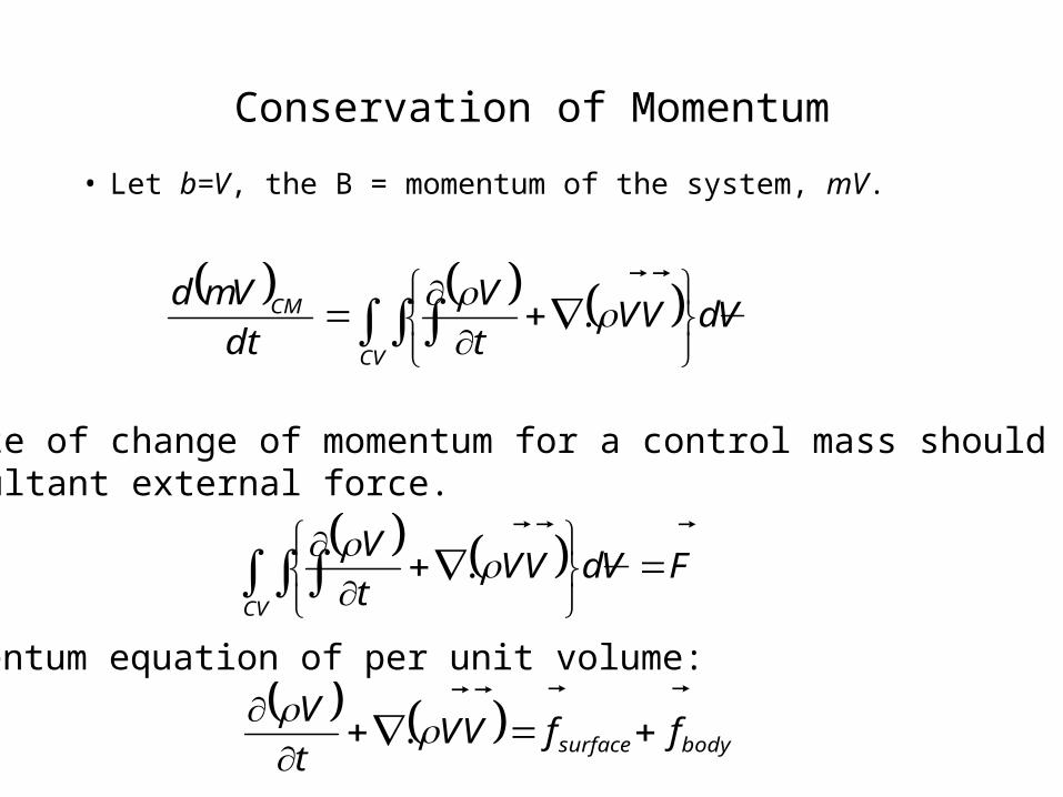
Conservation of Momentum
• Let b=V, the B = momentum of the system, mV.
The rate of change of momentum for a control mass should be equalto resultant external force.
CV
CM VdVVt
V
dt
Vmd
.
FVdVVt
V
CV
.
bodysurface ffVVt
V
.
Momentum equation of per unit volume:
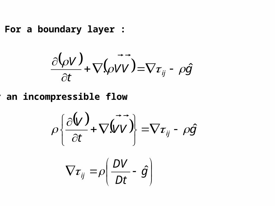
For a boundary layer :
gVVt
Vij ˆ..
For an incompressible flow
gVVt
Vij ˆ..
g
Dt
DVij ˆ.

Conservation of Energy
• Let b=e, the B = Energy of the system, me.
The rate of change of energy of a control mass should be equalto difference of work and heat transfers.
CV
CM VdVet
e
dt
dE
.
WQVdVet
e
CV
.
Energy equation per unit volume:
wqVet
e
.

Tkq .
Using the law of conduction heat transfer:
The net Rate of work done on the element is:
ijVw ..
From Momentum equation: N S Equations
g
Dt
DVij ˆ.
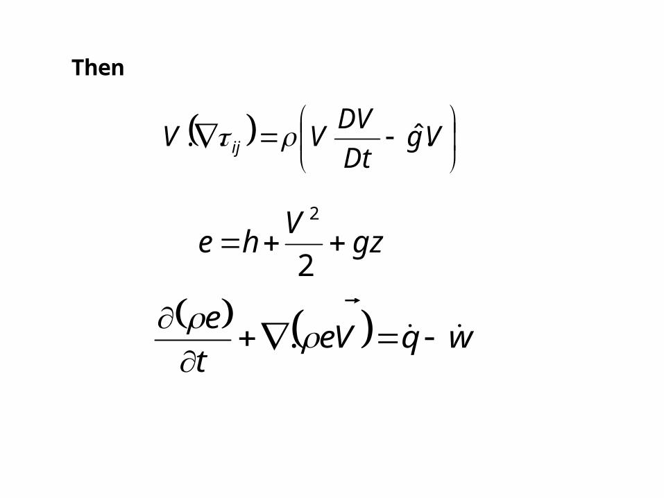
Then
Vg
Dt
DVVV ij .ˆ..
gzV
he 2
2
wqVet
e
.

j
iijij x
uVTkVg
Dt
DVV
Dt
Dh ....
j
iij x
uVg
Dt
DVVTkVg
Dt
DVV
Dt
Dh .ˆ..
Substitute the work done by shear stress:
j
iij x
uTk
Dt
Dh .
This is called the first law of thermodynamics for fluid motion.
For an Incompressible fluid:

Vpx
u
x
u
j
i
j
iij ij
.'
Dt
DpVp .
Invoking conservation of mass:
j
iij x
uTk
Dt
Dh .
First law for a fluid motion:
0. VDt
D
Dt
Dp
x
uTk
Dt
Dh
j
iij
'.
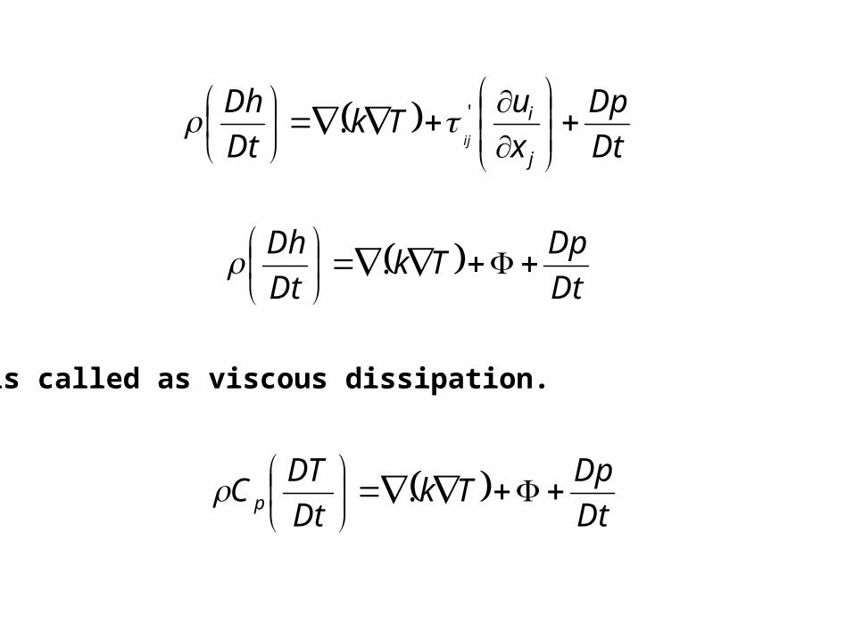
Dt
DpTk
Dt
Dh
.
is called as viscous dissipation.
Dt
DpTk
Dt
DTC p
.

Boundary Layer Equations
Consider the flow over a parallel flat plate.
Assume two-dimensional, incompressible, steady flow with constant properties.
Neglect body forces and viscous dissipation.
The flow is nonreacting and there is no energy generation.

The governing equations for steady two dimensional incompressible fluid flow with negligible viscous dissipation:

Boundary Conditions
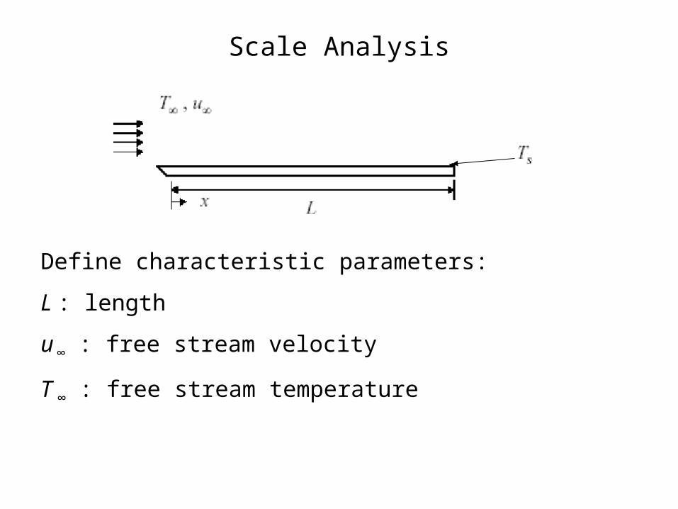
Scale Analysis
Define characteristic parameters:
L : length
u ∞ : free stream velocity
T ∞ : free stream temperature

General parameters:
x, y : positions (independent variables)
u, v : velocities (dependent variables)
T : temperature (dependent variable)
also, recall that momentum requires a pressure gradient for the movement of a fluid:
p : pressure (dependent variable)
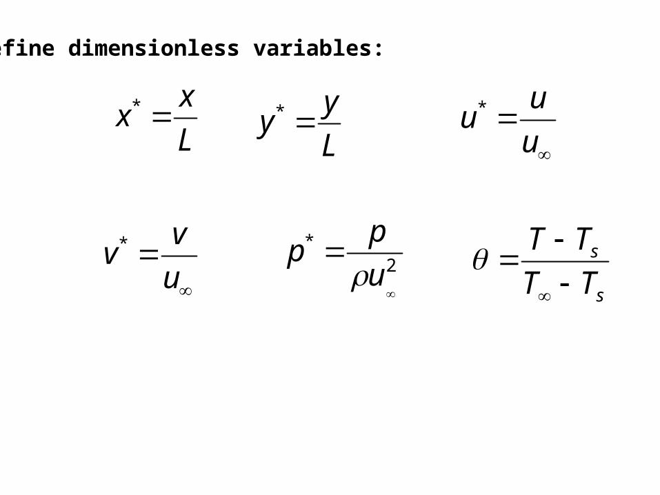
Define dimensionless variables:
L
xx *
L
yy *
u
uu*
u
vv*
s
s
TT
TT
2*
u
pp
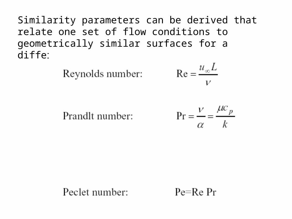
Similarity parameters can be derived that relate one set of flow conditions to geometrically similar surfaces for a different set of flow conditions:

0*
*
*
*
y
v
x
u
2*
*2
*
*
*
**
*
**
Re
1
y
u
x
p
y
vv
x
uu
L
2*
2
**
**
PrRe
1
yyv
xu
L
Boundary Layer Parameters
• Three main parameters (described below) that are used to characterize the size and shape of a boundary layer are:
• The boundary layer thickness,
• The displacement thickness, and
• The momentum thickness.
• Ratios of these thicknesses describe the shape of the boundary layer.

Boundary Layer Thickness
• The boundary layer thickness, signified by , is simply the thickness of the viscous boundary layer region.
• Because the main effect of viscosity is to slow the fluid near a wall, the edge of the viscous region is found at the point where the fluid velocity is essentially equal to the free-stream velocity.
• In a boundary layer, the fluid asymptotically approaches the free-stream velocity as one moves away from the wall, so it never actually equals the free-stream velocity.
• Conventionally (and arbitrarily), we define the edge of the boundary layer to be the point at which the fluid velocity equals 99% of the free-stream velocity:

• Because the boundary layer thickness is defined in terms of the velocity distribution, it is sometimes called the velocity thickness or the velocity boundary layer thickness.
• Figure illustrates the boundary layer thickness. There are no general equations for boundary layer thickness.
• Specific equations exist for certain types of boundary layer.
• For a general boundary layer satisfying minimum boundary conditions:
0 ;)( ;0)0(
y
y
uuuu
The velocity profile that satisfies above conditions:
2
22
yy
uu

Further analysis shows that:
xx Re
5.5
Where:
xu
xRe

Variation of Reynolds numbers
All Engineering Applications
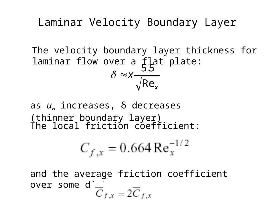
Laminar Velocity Boundary Layer
The velocity boundary layer thickness for laminar flow over a flat plate:
as u∞ increases, δ decreases (thinner boundary layer)
The local friction coefficient:
and the average friction coefficient over some distance x:
x
xRe
5.5

Laminar Thermal Boundary Layer
022
2
d
df
pr
d
d
Boundary conditions:
1 00
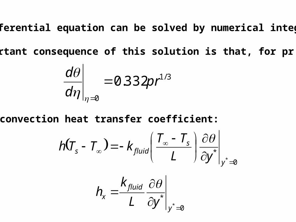
This differential equation can be solved by numerical integration.
One important consequence of this solution is that, for pr >0.6:
3/1
0
332.0 prd
d
Local convection heat transfer coefficient:
0
**
y
fluidx yL
kh
0
**
y
sfluids yL
TTkTTh

Local Nusselt number:
0
x
ukh fluidx
000
Re
xfluid
xx
xu
x
ux
k
xhNu
3/1Re332.0 prk
xhNu x
fluid
xx
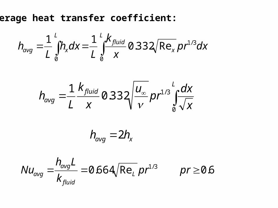
Average heat transfer coefficient:
L
xfluid
L
xavg dxprx
k
Ldxh
Lh
0
3/1
0
Re332.011
L
fluidavg
x
dxpr
u
x
k
Lh
0
3/1332.01
xavg hh 2
6.0 Re664.0 3/1 prprk
LhNu L
fluid
avgavg
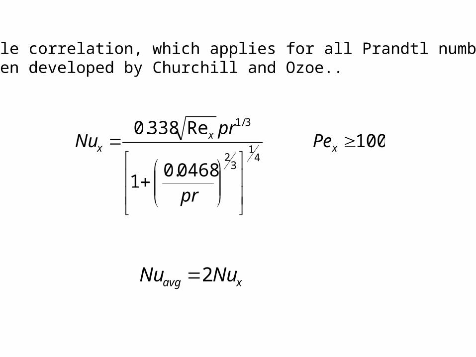
A single correlation, which applies for all Prandtl numbers,Has been developed by Churchill and Ozoe..
100
0468.01
Re338.0
41
32
3/1
xx
x Pe
pr
prNu
xavg NuNu 2

Turbulent Flow
• For a flat place boundary layer becomes turbulent at Rex ~ 5 X 10⁵.
• The local friction coefficient is well correlated by an expression of the form
7x
51
, 10Re Re059.0
xxfC
Local Nusselt number: 60 0.6 Re029.0 3/154
prprNu xx
Local Sherwood number: 60 0.6 Re029.0 3/154
ScScSh xx