tice

ap latticed constant. It is the

ily realized

Physics Letters A 340 (2005) 170–174

www.elsevier.com/locate/pla

Controlling spatiotemporal chaos of coupled bistable map latsystems using constant bias

Li-Juan Yuea,b,∗, Ke Shena

a Department of Physics, Changchun University of Science and Technology, Changchun 130022, Chinab Department of Physics, Northeast Normal University, Changchun 130024, China

Received 7 December 2003; received in revised form 22 March 2005; accepted 29 March 2005

Available online 12 April 2005

Communicated by A.R. Bishop

Abstract

We demonstrate that the global and local constant bias can suppress spatiotemporal chaos in coupled bistable msystem by varying the bias strength. The results of numerical simulation present that the constant bias and the improvebias are suitable for not only the acousto–optic bistable map system but also the coupled bistable map lattice systembest advantage that these methods do not require a priori information of system dynamics, and they can also be easin many natural systems. 2005 Elsevier B.V. All rights reserved.

PACS: 05.45.Pq; 05.45.Ra; 05.45.Gg; 42.65.Sf

Keywords: Controlling spatiotemporal chaos; Constant bias; Coupled bistable map lattice system

on-

non-h-

po-

rac-m-

m-hedi-

ms

e

1. Introduction

Since Ott, Grebogi and Yorke proposed the ctrolling chaos method (in short OGY)[1], controllingchaos has been one of attractive research fields oflinear dynamics. All kinds of controlling chaos metods have been proposed[2–12]. Controlling hyper-chaos in high dimension and controlling spatiotem

* Corresponding author.E-mail address: ljyue@nenu.edu.cn(L.-J. Yue).

0375-9601/$ – see front matter 2005 Elsevier B.V. All rights reserveddoi:10.1016/j.physleta.2005.03.063

ral chaos are challenging fields. There are many ptical nonlinear systems where both spatial and teporal chaos all exit. Controlling complex spatioteporal chaos, however, is still in an early stage. Tspatiotemporal chaos has been controlled in onemension unimodal logist coupled map lattice systeusing linear pinning feedback[13,14]global and localfeedback technique[15] constant pinning bias1 [16]adaptive controlling technique[17] and phase spac

1 This method is called constant feedback in the literature.

.

L.-J. Yue, K. Shen / Physics Letters A 340 (2005) 170–174 171

–aos

sta-iasagegeny

ely

pa-ral

s,

h-.blehe

to–pticm-

lu-as

m;er)ande

theayhan

od

c

-

iven

ngth

nri-

hefor

tem

-

compress[18]. We firstly control chaos in acoustooptical bistable map system and spatiotemporal chin coupled bistable map lattice systems to theble periodic orbits or the fixed point by constant band improved constant bias. It is the best advantthat constant bias controlling requires no knowledof system dynamics. It can be easily realized in manatural systems.

2. Coupled bistable map lattice model

It is caused extensive concern that the relativsimple coupled map lattice (CML) model[19,20] isa convenient tool to study the characteristics of stiotemporal chaos. The CML model is the geneform

xn+1(i) = (1− ε)f(xn(i)

)

(1)+ ε

2

(f

(xn(i + 1)

) + f(xn(i − 1)

)),

where n = 1,2, . . . ,N are the discrete time stepi = 1,2, . . . ,L are the lattice sites andL is the sys-tem size,ε is coupling strength to the nearest neigbor sites, andf (x) is the local dynamical functionHeref (x) is chosen to be the acousto–optic bistamap system, andx represents the state variable of tacousto–optic bistable map system. We call Eq.(1) asthe coupled bistable map lattice model. The acousoptic bistable device consists of laser, acousto–omodulator, driving source, photodiode, electronic aplifier and electronic delay line. In theory, the evotion of the acousto–optic bistability is representedfollowing [21]

(2)

τ0dx(t)

dt+ x(t) = π

{A − µsin2[x(t − τd) − xb

]},

wherex(t) is the state variable of the bistable systeµ is the bifurcation parameter (controlling parametthat decides the evolution of the bistable system,it is proportional to the input light intensity and thgain of the electronic amplifier;A andxb are constantsrelated to the voltages offset of the amplifier anddriver; τ0 and τd are the respond time and the deltime. If the respond time becomes much faster tthe delay time(τ � τ ), the dynamical Eq.(2) can be

0 d

represented the map equation

(3)xn+1 = π[A − µsin2(xn − xb)

],

where the parameters arexb = π4 , A = 0.5 at Eq.(3),

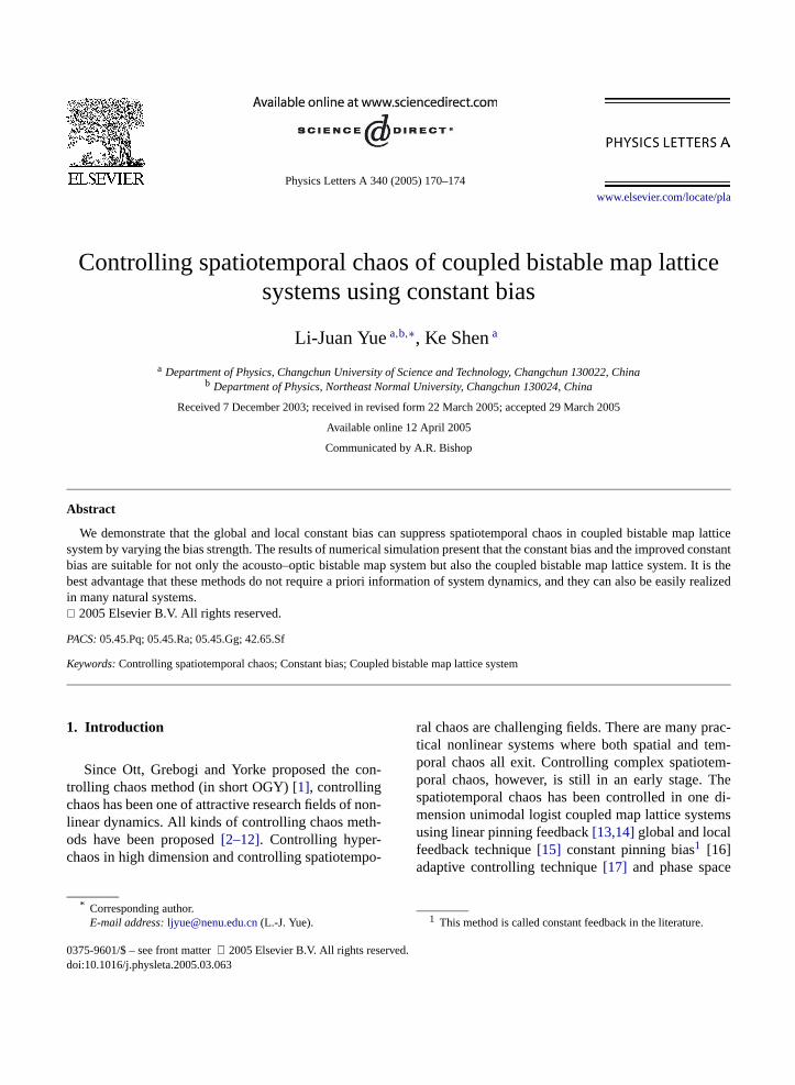
the bifurcation diagram ofxn versusµ is plotted inFig. 1. It is shown that the system varies from peridouble to chaos at differentµ. When the Lyapunovexponent is 0.72581 atµ = 0.9, the acousto–optibistable system is chaotic.

3. Controlling chaos in the acousto–optic bistablesystem

We apply constant bias[12] the acousto–opticbistable system. A constantk is added to the righthand side of Eq.(3) at each iteration having the form

(4)xn+1 = π[A − usin2(xn − xb)

] + k,

wherek is bias strength, the parameter values are gxb = π

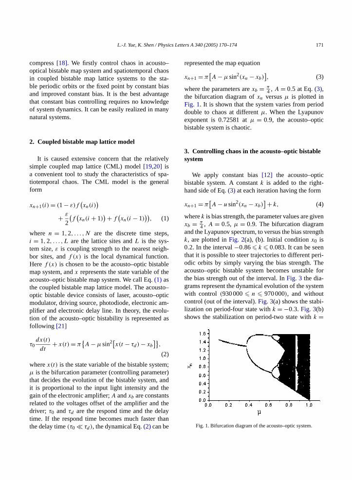
4 , A = 0.5, µ = 0.9. The bifurcation diagramand the Lyapunov spectrum, to versus the bias strek, are plotted inFig. 2(a), (b). Initial conditionx0 is0.2. In the interval−0.86� k � 0.083. It can be seethat it is possible to steer trajectories to different peodic orbits by simply varying the bias strength. Tacousto–optic bistable system becomes unstablethe bias strength out of the interval. InFig. 3 the dia-grams represent the dynamical evolution of the syswith control (930 000� n � 970 000), and withoutcontrol (out of the interval).Fig. 3(a) shows the stabilization on period-four state withk = −0.3. Fig. 3(b)shows the stabilization on period-two state withk =

Fig. 1. Bifurcation diagram of the acousto–optic system.

172 L.-J. Yue, K. Shen / Physics Letters A 340 (2005) 170–174

ne

uni-blethe

forwith

at

s

le

lps

ibitwo

un-

theledics

sara-.dif-e

−0.4. Fig. 3(c) shows the stabilization on period-ostate withk = −0.7.

4. Controlling turbulence in coupled bistable maplattice system

Spatiotemporal chaos is suppressed with theform constant bias technique in the coupled bistamap lattice system. The controlled dynamics under

Fig. 2. (a) Bifurcation diagram and (b) Lyapunov spectrumthe acousto–optic bistable system subjected to constant bias−0.86� k � 0.083.

influence of this bias is represent by

xn+1(i) = (1− ε)f(xn(i)

) + ε

2

(f

(xn(i + 1)

)

(5)+ f(xn(i − 1)

)) + k,

where the constantk shows the same bias strengthevery iteration. The local dynamical functionf (x) isthe acousto–optic bistable system of Eq.(3). The sys-tem parameters arexb = π

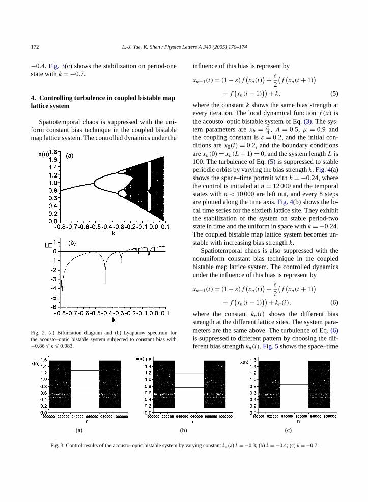
4 , A = 0.5, µ = 0.9 andthe coupling constant isε = 0.2, and the initial con-ditions arex0(i) = 0.2, and the boundary conditionarexn(0) = xn(L + 1) = 0, and the system lengthL is100. The turbulence of Eq.(5) is suppressed to stabperiodic orbits by varying the bias strengthk. Fig. 4(a)shows the space–time portrait withk = −0.24, wherethe control is initialed atn = 12 000 and the temporastates withn < 10 000 are left out, and every 8 steare plotted along the time axis.Fig. 4(b) shows the lo-cal time series for the sixtieth lattice site. They exhthe stabilization of the system on stable period-tstate in time and the uniform in space withk = −0.24.The coupled bistable map lattice system becomesstable with increasing bias strengthk.

Spatiotemporal chaos is also suppressed withnonuniform constant bias technique in the coupbistable map lattice system. The controlled dynamunder the influence of this bias is represent by

xn+1(i) = (1− ε)f(xn(i)

) + ε

2

(f

(xn(i + 1)

)

(6)+ f(xn(i − 1)

)) + kn(i),

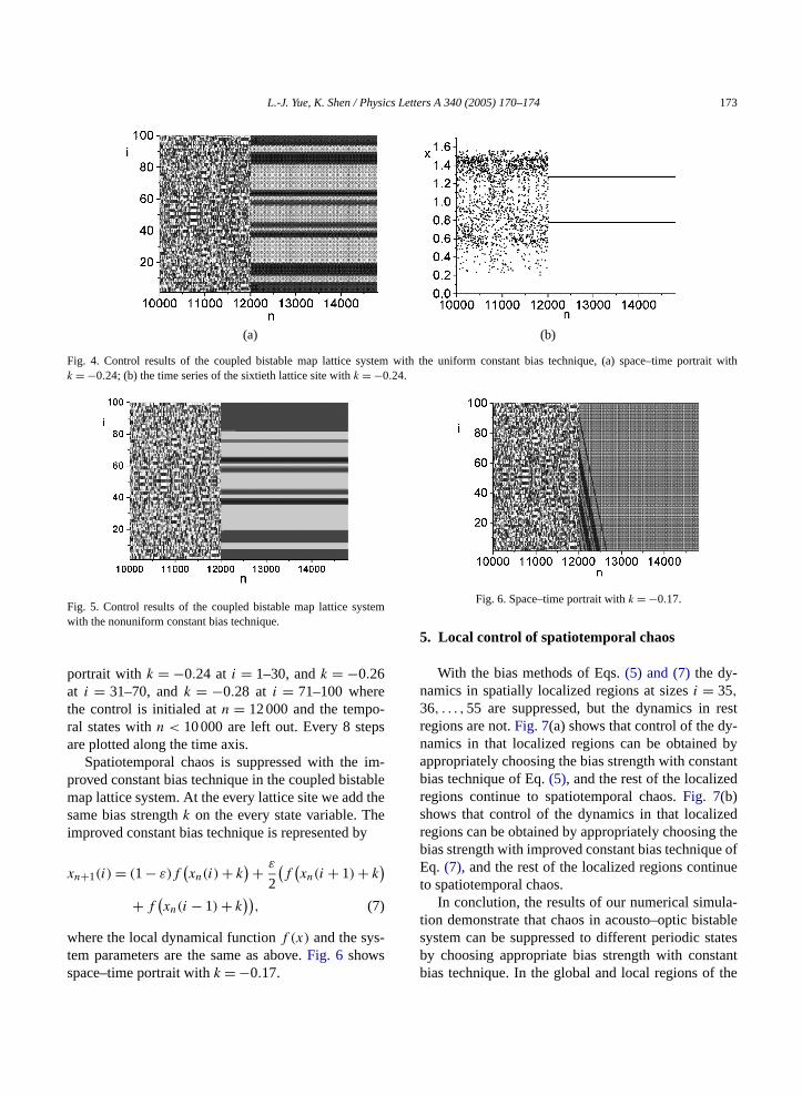
where the constantkn(i) shows the different biastrength at the different lattice sites. The system pmeters are the same above. The turbulence of Eq(6)is suppressed to different pattern by choosing theferent bias strengthk (i). Fig. 5shows the space–tim

n

(a) (b) (c)

Fig. 3. Control results of the acousto–optic bistable system by varying constantk, (a)k = −0.3; (b) k = −0.4; (c) k = −0.7.

L.-J. Yue, K. Shen / Physics Letters A 340 (2005) 170–174 173

rtrait with

(a) (b)

Fig. 4. Control results of the coupled bistable map lattice system with the uniform constant bias technique, (a) space–time pok = −0.24; (b) the time series of the sixtieth lattice site withk = −0.24.

tem

-s

im-abletheey

rest-by

tantd

edthe

e ofue

la-ableatestantthe

Fig. 5. Control results of the coupled bistable map lattice syswith the nonuniform constant bias technique.

portrait with k = −0.24 at i = 1–30, andk = −0.26at i = 31–70, andk = −0.28 at i = 71–100 wherethe control is initialed atn = 12 000 and the temporal states withn < 10 000 are left out. Every 8 stepare plotted along the time axis.

Spatiotemporal chaos is suppressed with theproved constant bias technique in the coupled bistmap lattice system. At the every lattice site we addsame bias strengthk on the every state variable. Thimproved constant bias technique is represented b

xn+1(i) = (1− ε)f(xn(i) + k

) + ε

2

(f

(xn(i + 1) + k

)

(7)+ f(xn(i − 1) + k

)),

where the local dynamical functionf (x) and the sys-tem parameters are the same as above.Fig. 6 showsspace–time portrait withk = −0.17.

Fig. 6. Space–time portrait withk = −0.17.

5. Local control of spatiotemporal chaos

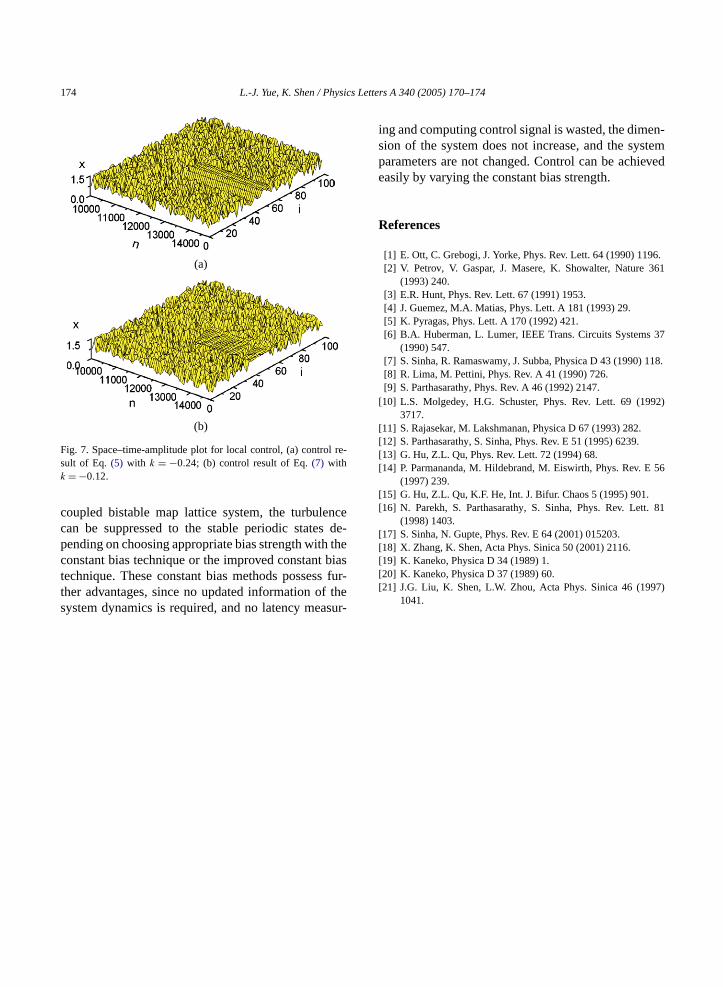
With the bias methods of Eqs.(5) and (7)the dy-namics in spatially localized regions at sizesi = 35,36, . . . ,55 are suppressed, but the dynamics inregions are not.Fig. 7(a) shows that control of the dynamics in that localized regions can be obtainedappropriately choosing the bias strength with consbias technique of Eq.(5), and the rest of the localizeregions continue to spatiotemporal chaos.Fig. 7(b)shows that control of the dynamics in that localizregions can be obtained by appropriately choosingbias strength with improved constant bias techniquEq. (7), and the rest of the localized regions continto spatiotemporal chaos.

In conclution, the results of our numerical simution demonstrate that chaos in acousto–optic bistsystem can be suppressed to different periodic stby choosing appropriate bias strength with consbias technique. In the global and local regions of

174 L.-J. Yue, K. Shen / Physics Letters A 340 (2005) 170–174

re-

ncede

thebias

furthesur-

en-tem

eved

6.61

37

118.

92)

56

. 81

7)

(a)

(b)

Fig. 7. Space–time-amplitude plot for local control, (a) controlsult of Eq. (5) with k = −0.24; (b) control result of Eq.(7) withk = −0.12.

coupled bistable map lattice system, the turbulecan be suppressed to the stable periodic statespending on choosing appropriate bias strength withconstant bias technique or the improved constanttechnique. These constant bias methods possessther advantages, since no updated information ofsystem dynamics is required, and no latency mea

-

-

ing and computing control signal is wasted, the dimsion of the system does not increase, and the sysparameters are not changed. Control can be achieasily by varying the constant bias strength.

References

[1] E. Ott, C. Grebogi, J. Yorke, Phys. Rev. Lett. 64 (1990) 119[2] V. Petrov, V. Gaspar, J. Masere, K. Showalter, Nature 3

(1993) 240.[3] E.R. Hunt, Phys. Rev. Lett. 67 (1991) 1953.[4] J. Guemez, M.A. Matias, Phys. Lett. A 181 (1993) 29.[5] K. Pyragas, Phys. Lett. A 170 (1992) 421.[6] B.A. Huberman, L. Lumer, IEEE Trans. Circuits Systems

(1990) 547.[7] S. Sinha, R. Ramaswamy, J. Subba, Physica D 43 (1990)[8] R. Lima, M. Pettini, Phys. Rev. A 41 (1990) 726.[9] S. Parthasarathy, Phys. Rev. A 46 (1992) 2147.

[10] L.S. Molgedey, H.G. Schuster, Phys. Rev. Lett. 69 (193717.

[11] S. Rajasekar, M. Lakshmanan, Physica D 67 (1993) 282.[12] S. Parthasarathy, S. Sinha, Phys. Rev. E 51 (1995) 6239.[13] G. Hu, Z.L. Qu, Phys. Rev. Lett. 72 (1994) 68.[14] P. Parmananda, M. Hildebrand, M. Eiswirth, Phys. Rev. E

(1997) 239.[15] G. Hu, Z.L. Qu, K.F. He, Int. J. Bifur. Chaos 5 (1995) 901.[16] N. Parekh, S. Parthasarathy, S. Sinha, Phys. Rev. Lett

(1998) 1403.[17] S. Sinha, N. Gupte, Phys. Rev. E 64 (2001) 015203.[18] X. Zhang, K. Shen, Acta Phys. Sinica 50 (2001) 2116.[19] K. Kaneko, Physica D 34 (1989) 1.[20] K. Kaneko, Physica D 37 (1989) 60.[21] J.G. Liu, K. Shen, L.W. Zhou, Acta Phys. Sinica 46 (199

1041.