WORKING PAPER SERIES

Controlling for Heterogeneity in Gravity Models of Trade and Integration

I-Hui Cheng and

Howard J. Wall

Working Paper 1999-010E http://research.stlouisfed.org/wp/1999/1999-010.pdf

Revised July 2004

FEDERAL RESERVE BANK OF ST. LOUIS

Research Division 411 Locust Street

St. Louis, MO 63102

______________________________________________________________________________________

The views expressed are those of the individual authors and do not necessarily reflect official positions of the Federal Reserve Bank of St. Louis, the Federal Reserve System, or the Board of Governors.

Federal Reserve Bank of St. Louis Working Papers are preliminary materials circulated to stimulate discussion and critical comment. References in publications to Federal Reserve Bank of St. Louis Working Papers (other than an acknowledgment that the writer has had access to unpublished material) should be cleared with the author or authors.

Photo courtesy of The Gateway Arch, St. Louis, MO. www.gatewayarch.com

Controlling for Heterogeneity in Gravity Modelsof Trade and Integration

I-Hui ChengNational University of Kaohsiung, Taiwan

Howard J. WallFederal Reserve Bank of St. Louis, USA

revised July 2004

This paper compares various specifications of the gravity model of trade as nested versions of ageneral specification that uses bilateral country-pair fixed effects to control for heterogeneity.For each specification, we show that the atheoretical restrictions to obtain them from the generalmodel are not supported statistically. Because the gravity model has become the ‘workhorse’baseline model for estimating the effects of international integration, this has important empiricalimplications. In particular, we show that, unless heterogeneity is accounted for correctly, gravitymodels can greatly overestimate the effects of integration on the volume of trade. (JEL F15,F17)

Corresponding author: Howard J. Wall, Research Division, Federal Reserve Bank of St.Louis, P.O. Box 442, St. Louis, MO 63166-0442, United States. E-mail: wall@stls.frb.org;Phone: (314)444-8533; Fax: (314)444-8731

We would like to thank Martin Sola, Ron Smith, Jim Dunlevy, and Rob Dittmar for theircomments and suggestions. Kristie Engemann provided research assistance. The viewsexpressed are those of the authors and do not necessarily represent official positions of theFederal Reserve Bank of St. Louis or of the Federal Reserve System.

1

Controlling for Heterogeneity in Gravity Modelsof Trade and Integration

1. Introduction

Starting in the 1860s when H. Carey first applied Newtonian Physics to the study of

human behavior, the so-called “gravity equation” has been widely used in the social sciences.

More recently, gravity model studies have achieved empirical success in explaining various

types of inter-regional and international flows, including labor migration, commuting, customers,

hospital patients, and international trade. The widespread use of gravity equations is despite the

fact that they have, until recently, tended to lack strong theoretical bases.

The gravity model of international trade was developed independently by Tinbergen

(1962) and Pöyhönen (1963). In its basic form, the amount of trade between two countries is

assumed to be increasing in their sizes, as measured by their national incomes, and decreasing in

the cost of transport between them, as measured by the distance between their economic centers.1

Following this work, Linnemann (1966) included population as an additional measure of country

size, employing what we will call the augmented gravity model.2 It is also common to instead

specify the augmented model using per capita income, which captures the same effects.3

Whichever specification of the augmented model is used, the purpose is to allow for non-

homothetic preferences in the importing country, and to proxy for the capital/labor ratio in the

exporting country (Bergstrand, 1989).

1 For examples see McCallum (1995), Helliwell (1996), and Boisso and Ferrantino (1997).2 For uses of the augmented gravity model, see Oguledo and MacPhee (1994), Boisso and Ferrantino (1997), andBayoumi and Eichengreen (1997).3 Examples of the augmented model with per capita income include Sanso, Cuairan, and Sanz (1993), Frankel andWei (1998), Frankel, Stein, and Wei (1995, 1998), Eichengreen and Irwin (1998).

2

The gravity model has been used widely as a baseline model for estimating the impact of

a variety of policy issues, including regional trading groups, currency unions, political blocs,

patent rights, and various trade distortions.4 Typically, these events and policies are modeled as

deviations from the volume of trade predicted by the baseline gravity model, and, in the case of

regional integration, are captured by dummy variables. The recent popularity of the gravity

model is highlighted by Eichengreen and Irwin (1998, p.33) who call it the “workhorse for

empirical studies of [regional integration] to the virtual exclusion of other approaches.”

The perceived empirical success of the gravity model has come without a great deal of

analysis regarding its econometric properties, as its empirical power has usually been stated

simply on the basis of goodness of fit; i.e. a relatively high 2R .5 The lack of attention paid to

the empirical properties of the model is despite the fact that the strength of any baseline model

lies in the accuracy of its estimates. Recently, though, several papers have argued that standard

cross-sectional methods yield biased results because they do not control for heterogeneous

trading relationships. Because of this, these papers introduced fixed effects into the gravity

equation. Fixed-effects models allow for unobserved or misspecified factors that simultaneously

explain trade volume between two countries and, for example, the probability that the countries

will be in the same regional integration regime (Mátyás, 1997; Bayoumi and Eichengreen, 1997;

Cheng, 1999; Wall, 2002 and 2003; Coughlin and Wall, 2003).6 They have also been used by

Glick and Rose (2001) and Pakko and Wall (2001) to estimate the trade effects of currency 4 See Aitken (1973), Brada and Mendez (1983), Bikker (1987), Sanso, Cuairan, and Sanz (1993), McCallum (1995),Helliwell (1996), Frankel (1997), Wei and Frankel (1997), Bayoumi and Eichengreen (1997), Mátyás (1997),Frankel and Wei (1998), Frankel, Stein, and Wei (1998), Smith (1999), Rose (2000).5 See Sanso, Cuairan, and Sanz (1993) for an examination of the predictive power of various specifications of theaugmented gravity model. Also, see Oguledo and MacPhee (1994) for a survey of pre-1990 empirical results.6 Soloaga and Winters (2001) also recognize this problem, but their solution is to estimate yearly gravity models andto calculate the effects of integration as the differences in the predicted trade volumes over time.

3

unions; by Wall (2000) and Millimet and Osang (2004) to estimate the effects of borders on

trade; by Egger (2002) to calculate trade potentials; and by Wall (1999) to estimate the costs of

protection.

Although the arguments underlying the use of fixed effects as a solution to unobserved

heterogeneity are roughly the same in all of these papers, there is little agreement about how to

actually specify the fixed effects. For example, Cheng (1999) and Wall (1999) propose two

fixed effects for each pair of countries, one for each direction of trade. In Glick and Rose

(2001), each pair of countries has only one fixed effect. In Mátyás (1997), each country has two

fixed effects, one as an exporter and one as an importer. The purpose of this paper is to evaluate

the various fixed-effect specifications in terms of the econometric appropriateness of their

underlying assumptions. Specifically, we show how the standard pooled-cross-section

specification and other fixed-effects specifications are special cases of the Cheng (1999) and

Wall (1999) specification, and that these restrictions to obtain them cannot be supported

empirically. To underscore the importance of getting the fixed-effects specification right, we

illustrate how the choice of specification has significant implications when estimating the effects

of integration on trade volume.

Section 2 briefly sets out the various statistical models we examine. Section 3 presents

standard empirical results for the augmented gravity model and demonstrates its inherent

heterogeneity bias. In Section 4, we specify a general fixed-effects gravity model. In Section 5,

we compare fixed-effects specifications that are nested versions of the general one. Section 6

illustrates the importance of fixed-effects estimation when estimating the effects of trade blocs.

Section 7 concludes.

4

2. A Statistical Overview

This section briefly sets out the various forms of the gravity model that have been used to

estimate bilateral trade flows. These models are restricted versions of a general gravity model,

which has a log-linear specification but places no restrictions on the parameters. In the general

model, the volume of trade between countries i and j in year t can be characterized by

,ln 0 ijtijtijtijtX ε+′+α+α+α= Zβ ijt t = 1,…,T; (1)

where ijtX is exports from country i to country j in year t, and ijtZ′ = [ ... jtit zz ] is the 1 × k

row vector of gravity variables (GDP, population, and distance). The intercept has three parts,

one which is common to all years and country pairs, 0α , one which is specific to year t and

common to all pairs, tα , and one which is specific to the country pairs and common to all years,

ijα . The disturbance term ijtε is assumed to be normally distributed with zero mean and

constant variance for all observations. It is also assumed that the disturbances are pairwise

uncorrelated.

Obviously, because (1) has only one observation, it is not useful for estimation unless

restrictions are imposed on the parameters. The standard single-year cross-section model (CS)

imposes the restrictions that the slopes and intercepts are the same across country pairs; i.e., that

0=ijα and tijt ββ = ,

,ln 0 ijttijtX ε+′+α+α= ijtt Zβ t = 1, ..., T; (CS)

where 0α and tα cannot be separated. Assuming that all the classical disturbance-term

assumptions hold, the CS model is estimated by ordinary least squares (OLS) for each year.

5

The other standard estimation method is a pooled-cross-section model (PCS), which

imposes the further restriction on the general model that the parameter vector is the same for all

t, == 21 ββ ... ββT == , although it normally allows the intercepts to differ over time;

,ln 0 ijttijtX ε+′+α+α= ijtZβ t = 1, ..., T. (PCS)

This is estimated by OLS using data for all available years.

Nearly all estimates of the gravity model of trade use either the CS or the PCS model,

which, as we show below, both provide biased estimates. To address this bias, we remove the

restriction that the country-pair intercept terms equal zero, although we maintain the restriction

that the slope coefficients are constant across country pairs and over time. Specifically, we

estimate the fixed-effects (FE) model of Cheng (1999) and Wall (1999):

,ln 0 ijtijtijtX ε+′+α+α+α= ijtZβ t = 1, ..., T. (FE)

Note that the country-pair effects are allowed to differ according to the direction of trade, i.e.,

jiij α≠α . The FE model is a two-way fixed-effects model in which the independent variables

are assumed to be correlated with ijα , and is a classical regression model that can be estimated

using LSDV (least squares with a dummy variable for each of the country pairs).

As mentioned above, others have proposed alternative fixed-effects models to handle

country-pair heterogeneity, each of which can be modeled as a restricted version of the FE model

above. The symmetric fixed-effects (SFE) model of Glick and Rose (2001) differs from FE only

in that it imposes the restriction that the country-pair effects are symmetric, i.e., jiij α=α .

In the Bayoumi and Eichengreen (1997) model, call it DFE, the differences in the

dependent and independent variables are used to eliminate the fixed variables, including the

6

country-pair dummies and distance. As with the FE specification, this model allows for the most

general fixed effects possible. But rather than estimating the fixed effects using LSDV, it

eliminates them by subtracting them out. Specifically,

0ln ,ijt t ijtX γ γ µ′∆ = + + ∆ +ijtβ Z t = 1, ..., T; (DFE)

where ∆ is the difference operator, and 10 −α−α=γ+γ ttt . In this model the intercept has two

parts: 0γ is the change in the period-specific effect that is common across years, and tγ is the

change that is specific to year t.

When there are no time dummies, such a differencing model yields results identical to a

model with dummy variables to control for fixed effects. However, with time dummies it is

necessary to impose restrictions on the time effects so as to avoid collinearity, which in turn

makes the DFE estimation a restricted form of the FE estimation. If the collinearity restriction is

that the first time dummy in the DFE model is equal to zero, this is equivalent to restricting the

common component of the change in the period-specific effects as equal to the difference in the

first two period-specific effects, i.e., .120 α−α=γ If, instead, the collinearity restriction is that

the sum of the time dummies in the DFE model is zero, this is equivalent to restricting the

common component as equal to the difference between the first and last time dummies, i.e.,

.10 α−α=γ T

Mátyás (1997) proposes

,ln 0 ijtjitijtX ε+′+ω+θ+α+α= ijtZβ t = 1, ..., T; (XFE)

as the correct specification of the gravity model, where the country-specific effect when a

country is an exporter is iθ , and when it is an importer is jω . Note that in this specification,

7

distance, contiguity, and language are eliminated because they are fixed over time, even though

they are not collinear with the country-specific effects. This model is a special case of the FE

model in that it has a unique value for each trading pair’s intercept, with the restrictions that a

country’s fixed effect as an exporter or importer is the same for all of its trading partners. This

imposes cross-pair restrictions on the intercepts; i.e., one of the components of the intercept for

U.S.-to-Canada trade must be the same as one of the components of the intercept for U.S.-to-

France trade. These restrictions do not change the coefficient estimates very much, but, as we

show below, lead to biased and rather large residuals, indicating inaccurate in-sample predictions

of trade flows.

3. Standard Results

This section presents regression results for the augmented version of the standard pooled-

cross-section (PCS) model.7 The data set is a balanced panel with 3188 observations (797

unidirectional country-pairs in each of four years: 1982, 1987, 1992, and 1997).8 We included

observations of non-zero trade between countries listed in all of the relevant World Bank World

Development Reports as being upper-middle or high income during these years. Also, we

excluded countries that were identified as high-income oil exporters. The result is a manageable

data set that is fairly representative of the literature, which typically includes only OECD

members or industrialized countries. Descriptions of the data and their sources are provided in

the data appendix. 7 Because the results for the single-year CS do not differ substantially from those for the PCS model, we do notpresent them here. However, they are available upon request.

8

In the augmented version of the gravity model, the gravity variables are the countries’

GDPs, their populations, and the distance between them. Thus, the augmented PCS model

assumes that in a given year trade flows from exporting country i to importing country j can be

estimated using: 9

;lnlnlnlnlnln 2143210 ijtijijijjtitjtittijt LCDNNYYX ε+λ+δ+δ+β+β+β+β+α+α= (2)

where 0α is the portion of the intercept that is common to all years and trading pairs; tα denotes

the year-specific effect common to all trading pairs; iY and jY are the two countries’ GDPs;

iN and jN are their populations; ijD is the distance between them; ijC is a contiguity dummy;

and ijL is a common-language dummy. Note that our estimation omits the dummy for 1982 so

as to avoid collinearity.

Because trade flows are expected to be positively related to national incomes, and

negatively related to distance, 1β , 2β , and 2δ are expected to be positive, and 1δ is expected to

be negative. The signs expected for population coefficients are not as unambiguous, and the

literature has not tended to find a consistent sign for 43 or ββ .10 Because ijL is meant to capture

cultural and historical similarities between the trading pairs, which are thought to increase the

volume of trade, λ is expected to be positive. Finally, we take the time dummies as indicators of

the extent of “globalization”, which we define as the purported common trend towards greater

real trading volumes, independent of the sizes of the economies.

8 Fixed-effects estimation is sometimes criticized when applied to data pooled over consecutive years on thegrounds that dependent and independent variables cannot fully adjust in a single year’s time. To avoid this, we leftfive years between our observations.9 Note that because NYincomecapitaper lnln) ( ln −= , the regression could be suitably rearranged toinstead obtain the augmented model with per capita income.10 See Oguledo and MacPhee (1994).

9

The regression results for PCS are reported in the first column of Table 1. The signs of

the coefficients on distance, common language, and the countries’ GDPs are as expected, and are

statistically significant. Only the negative coefficient on the contiguity dummy of PCS is not as

expected, although it is not statistically different from zero. Perhaps surprisingly, the

coefficients on the time dummies do not indicate a trend towards globalization.

According to the estimates of the PCS model: (i) an increase in a country’s GDP will lead

to a less-than-proportional increase in its imports and exports and (ii) a country will export 103

percent more to a market that is half as distant as another otherwise-identical market, and 108

percent more to a country with the same first language. Finally, we take the fact that the time

dummies are not statistically different from zero to mean that globalization, as defined above,

was not an important factor in increasing trade over the period.

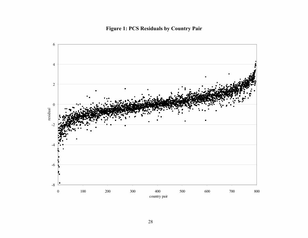
Despite the supposed empirical success that we have replicated, there is a severe problem

with the standard model. This is clear from Figure 1, which plots the residuals for the PCS

model for the 797 unidirectional country pairs in our data set, ordered by the pairs’ average

residuals. If the PCS estimation were unbiased, there would be no discernable pattern in Figure

1 because the average residual for each country pair would be zero. The residuals for 544 of the

country pairs, however, always have the same sign. In other words, the PCS model consistently

mis-estimated the volume of trade for 68 percent of the country pairs.

10

4. The Gravity Model with Country-Pair Fixed Effects

a. The model

Standard cross-section estimates of the gravity model yield biased estimates of the

volume of bilateral trade because there is no heterogeneity allowed for in the regression

equations. With such heterogeneity, a country would export different amounts to two countries,

even though the two export markets have the same GDPs and are equidistant from the exporter.

This can be because there are historical, cultural, ethnic, political, or geographic factors that

affect the level of trade, and are correlated with the gravity variables (GDP, population,

distance). If so, then estimates that do not account for these factors will suffer from

heterogeneity bias.

Some studies using the PCS model have to some extent tried to control for this by

including things such as whether trading partners share a common language, have had a colonial

history, are in military alliance, etc. However, cultural, historical, and political factors are often

difficult to observe, let alone quantify. This is why we will control for these factors using a

simple fixed-effects model that assumes that there are fixed pair-specific factors that may be

correlated with levels of bilateral trade and with the right-hand-side variables. It is in this sense

fixed-effects modeling is a result of ignorance: We do not have a good idea which variables are

responsible for the heterogeneity bias, so we simply allow each trading pair to have its own

dummy variable.

We assume that the gravity equation for a country pair may have a unique intercept, and

that it may be different for each direction of trade; i.e., jiij α≠α . However, we retain the

11

assumptions of the PCS model that the slope coefficients are constant over time and across

trading pairs. The Cheng (1999) and Wall (1999) specification of the augmented FE is:

;lnlnlnlnln 4321 ijtjtitjtittijijt NNYYX ε+β+β+β+β+α+α= (3)

where ijα is the specific “country-pair” effect between the trading partners. The country-pair

intercepts include the effects of all omitted variables that are cross-sectionally specific but

remain constant over time, such as distance, contiguity, language, culture, etc. Using the pooled

data described above, we have 797 country-pair intercepts.

Because there is a long-standing problem with determining the appropriate measure of

economic distance so as to capture transportation and information costs (see Head and Mayer,

2001, for a review of the issue), an added benefit of the fixed-effects model is that it eliminates

the need to include distance in the regression. The most common method for measuring distance

is to do as we have and simply measure it between the centers (often assumed to be the capital

cities) of the two countries. There are problems with this, such as the implicit assumptions that

overland transport costs are the same as those over sea, and that all overland/oversea distances

are equally costly. To provide just one example, Los Angeles is about 1300 kms farther from

Tokyo than is Moscow, but it is difficult to believe that the economic distance between Tokyo

and Los Angeles is not much lower than that between Tokyo and Moscow. Our fixed-effects

approach eliminates the need to include a distance variable, as it controls for all variables that do

not change over time.

Another difficulty with standard measures of economic distance is the common

assumption that the capital city, or any other single point in the country, is a useful proxy for the

12

economic center. While this may be useful for small countries with one major city, it is wide of

the mark for countries like Canada and the U.S., which have major cities thousands of miles

apart on different oceans, and which serve as centers for trade with completely different

countries. By using Washington, DC, or Ottawa to measure distance between the U.S. or

Canada and its Pacific trading partners is to overstate distance by the entire breadth of the North

American continent. As the U.S. has the highest GDP and the highest volume of trade, the mis-

measure of economic distance can bias the estimation of the coefficients on the other variables in

the gravity model.

Another advantage of our approach is that it removes the problem of controlling for

contiguity. Although it is potentially important, as a great deal of the trade can occur from

people crossing the border to make everyday purchases, it is accounted for only sometimes.

Even when it is accounted for with a dummy variable as we do above, it still assumes that all

contiguity is equivalent and time-invariant in terms of its effect on trade. Considering that

Canada and the U.S., China and Russia, and Argentina and Chile are all equivalently contiguous

pairs, this is difficult to abide by.

b. The results

Table 1 reports the estimation results for the augmented version of the FE model. Note

that for comparison with the pooled-cross-section results, the year dummies are measured

relative to that of 1982. Also, the estimates of the country-pair intercepts are omitted for space

considerations. According to the results for the FE model: (i) an increase in a country’s GDP

13

will lead to a less-than-proportional increase in its imports and exports; and (ii) globalization has

increased the real volume of trade by 48 percent between 1982 and 1997.

A comparison of the results of the FE and PCS models, shows that allowing for trading-

pair heterogeneity lowers the estimated income elasticities of trade, greatly increases the

absolute value of the coefficients on the countries’ populations, and greatly increases the

estimated role of globalization. It is obvious from the results that restricting the country-pair

effects to zero, as does the PCS model, has statistically significant effects on the results, as is

easily confirmed by a likelihood ratio test.11 Note also that the residuals from the FE estimation

across country pairs (Figure 2) have no discernible pattern.

Therefore, because the PCS model is a restricted form of the FE model, and the

restrictions are not supported statistically, we conclude that the FE model is the preferred

specification of the gravity model. In short, there is no statistical support for imposing the

parameter restrictions required by the standard procedures for estimating the gravity model of

trade. In the absence of any economic arguments for believing that the intercepts of the gravity

equation are the same across trading pairs, we conclude that the fixed-effects model is the more

appropriate specification.

Oddly, Wei and Frankel (1997, p.125) reject the inclusion of country-pair dummies a

priori on the basis that doing so would undermine their efforts at estimating the effects of

variables that are constant over the sample period. Presumably, their worry is that because these

variables are subsumed into the country-pair effects they are hidden from analysis. This is

unfounded because the effects of these variables are easily estimated by regressing them on the

11 This is with with LR = 7000.4 and χ2(796) = 862.75 at the 5-percent level.

14

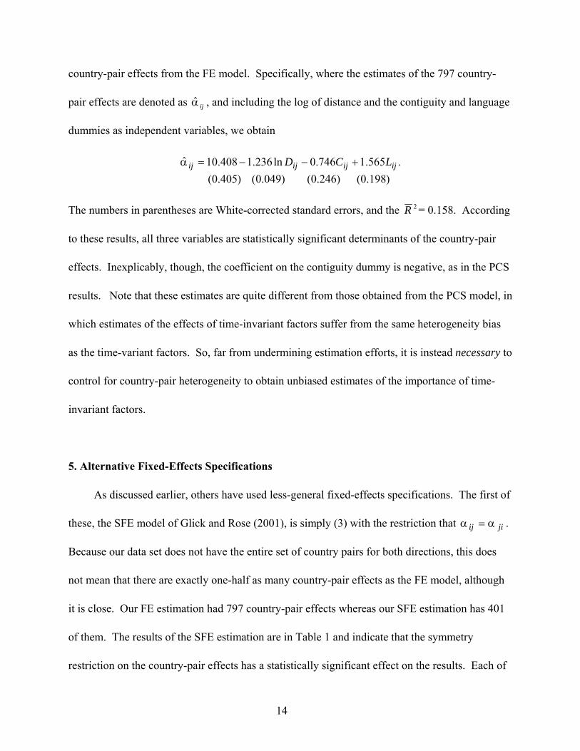
country-pair effects from the FE model. Specifically, where the estimates of the 797 country-

pair effects are denoted as ijα̂ , and including the log of distance and the contiguity and language

dummies as independent variables, we obtain

)198.0( )246.0( )049.0( )405.0( .565.1746.0ln236.1408.10ˆ ijijijij LCD +−−=α

The numbers in parentheses are White-corrected standard errors, and the 2R = 0.158. According

to these results, all three variables are statistically significant determinants of the country-pair

effects. Inexplicably, though, the coefficient on the contiguity dummy is negative, as in the PCS

results. Note that these estimates are quite different from those obtained from the PCS model, in

which estimates of the effects of time-invariant factors suffer from the same heterogeneity bias

as the time-variant factors. So, far from undermining estimation efforts, it is instead necessary to

control for country-pair heterogeneity to obtain unbiased estimates of the importance of time-

invariant factors.

5. Alternative Fixed-Effects Specifications

As discussed earlier, others have used less-general fixed-effects specifications. The first of

these, the SFE model of Glick and Rose (2001), is simply (3) with the restriction that jiij α=α .

Because our data set does not have the entire set of country pairs for both directions, this does

not mean that there are exactly one-half as many country-pair effects as the FE model, although

it is close. Our FE estimation had 797 country-pair effects whereas our SFE estimation has 401

of them. The results of the SFE estimation are in Table 1 and indicate that the symmetry

restriction on the country-pair effects has a statistically significant effect on the results. Each of

15

the coefficients on the gravity variables is very different from what we obtain with the FE model,

although the coefficients on the year dummies are nearly identical. Also, a likelihood ratio test

easily rejects the null hypothesis that the restrictions do not have a statistically significant effect

on the estimation.12 This means that the FE model is preferred statistically to the SFE model.

Taking the time difference of (3), the DFE model of Bayoumi and Eichengreen (1997) is

;lnlnlnlnln 43210 ijtjtitjtittijt NNYYX µ+∆β+∆β+∆β+∆β+γ+γ=∆ (4)

where the intercept is as defined in Section 2, 10 −α−α=γ+γ ttt . To prevent collinearity, we

set the time dummy for 1987 equal to zero, meaning that other time dummies are measured

relative to it. In terms of the more-general FE model, this is equivalent to restricting the

common component of the change in the period-specific effects as equal to the difference in the

first two period-specific effects; i.e., .120 α−α=γ 13 The empirical results are presented in

Table 1.

The results for the FE and DFE models are similar in terms of the signs and order of

magnitude of the coefficients. Nonetheless, the FE and DFE results differ enough to reject the

restrictions needed to obtain DFE model. This can be confirmed easily by a likelihood ratio test.

Therefore, given the restrictions that DFE imposes on the time dummies are not justified on any

economic or statistical grounds, our results indicate that they should not be imposed.

The third alternative to the FE model, XFE, is

;lnlnlnlnln 43210 ijtjtitjtitjitijt NNYYX ε+β+β+β+β+ω+θ+α+α= (5)

12 This is with LR = 2400.78 and χ2(395) = 442.34 at the 5-percent level.13 The alternative assumption that the sum of the year dummies is zero means that 10 α−α=γ T , and yields thesame results except for the time dummies and the constant.

16

where the fixed effect when a country is an exporter is iθ , and when it is an importer is jω .

One way to prevent perfect collinearity in estimating (5) is to impose the restrictions that one of

the θs and one of the ωs is zero. Because each iθ and jω comprise part of many sijα , this is

the same as imposing a series of cross-pair restrictions on the sijα . From the empirical results

summarized by the last column of Table 1, it seems that the coefficients are the same as those

from the FE model. In fact, the coefficients are not the same, but the differences are so small

that they appear only beyond the seventh decimal places provided by STATA. More

importantly, though, the standard errors from the XFE model are much larger. Consequently, the

FE model is preferred to the XFE model on the basis of any standard goodness-of-fit criteria. As

with the other restricted fixed-effects specifications, a likelihood ratio test easily rejects the null

hypothesis that the arbitrary restrictions imposed by XFE are not statistically benign.

6. The Effects of Integration

As we discuss in the Introduction, the gravity model has become the primary tool for

estimating the effects of regional integration on trade volumes. Up to this point, we have

omitted integration variables in order to focus on the importance of controlling for country-pair

heterogeneity when estimating gravity models. We now introduce integration into our model

and demonstrate the striking effect that heterogeneity bias has on the results. We would also like

to alleviate the valid concern that the heterogeneity bias we detected above was due to our

implicit assumption that regional integration is uncorrelated with the independent variables.

The most common and straightforward method for estimating the effects of integration in

a gravity model is to include dummy variables for each integration regime in place during the

17

sample period (see, for example, Frankel, 1997). Each of these dummies takes the value of 1 for

an observation for which the two countries are members of the regime, with the expectation that

the coefficients on these dummies are positive. We include five such dummy variables in our

model, one each for the European trading bloc, the North American trading bloc, the South

American trading bloc (Mercosur), the Australia-New Zealand Closer Economic Relations

(CER), and the Israel-U.S. Free Trade Agreement (FTA).

Although there has been some deepening of trade integration in the European bloc, the

primary change over the period was an expansion in the number of countries covered under the

customs union. The formation of the European Community (EC) predates our data set, and

Portugal and Spain joined in 1986. The twelve countries of the EC renamed themselves the

European Union (EU) in 1992, but this had relatively little effect on internal trade policy, as it

was already nearly unfettered under the EC. Expansion of the bloc came in 1994 with the

European Economic Area (EEA), which extended the free trade zone to include Austria, Iceland,

Finland, Norway, and Sweden. To capture the effect of this trading bloc, our European bloc

dummy variable takes the value of 1 when trade is between members of the EC or EU for 1982,

1987, 1992, and between members of the EEA for 1997.

The Canada-U.S. Trade Agreement of 1988 established a North American trading bloc

that included only Canada and the United States. The North American Free Trade Agreement

(NAFTA) expanded the free trade zone in 1994 to include Mexico. We ignore NAFTA’s

relatively mild deepening of U.S.-Canada integration, and focus instead on it as an extension of

the free trade bloc to Mexico. Our North American bloc dummy takes the value of 1 for trade

between the U.S. and Canada for 1992, and between Mexico, Canada, and the U.S. for 1997.

18

The third significant trade bloc during the period was Mercosur, which came into force in

1995, reducing trade barriers between Argentina, Brazil, Paraguay, and Uruguay. Our Mercosur

dummy takes the value of 1 for trade between any two of these countries in 1997. The Australia-

New Zealand CER was formed in 1983, so its dummy variable is equal to 1 for trade between the

two countries for all years but 1982. Similarly, the Israel-U.S. FTA entered into force in 1985,

so its dummy variable is equal to 1 for trade between the two countries for 1987, 1992, and 1997.

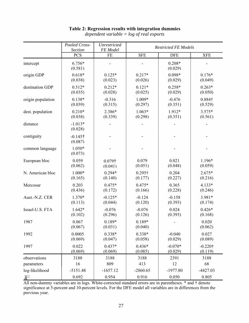
We include these trade bloc dummies in the PCS and FE models, and report the empirical

results in Table 2. Note that inclusion of these dummies makes little difference for the PCS

model. Nonetheless, a likelihood ratio test rejects the null hypotheses that including the trade

bloc dummies in the PCS model does not alter the results to a statistically significant extent.14

Similarly, the results for the FE model are also not dramatically different when the trade bloc

dummies are included, although the null hypothesis that the inclusion of these variables has no

statistically significant effect on the results can be rejected.15

Both models find modest effects on trade from the European trade bloc. The PCS

estimates say that the bloc had a statistically insignificant effect but the FE estimates say that it

had a statistically significant effect of 8.2 percent (e0.079-1 = 0.082). The larger differences

between the two models are in the estimated effects of the other trade blocs. The PCS model

suggests a 172-percent increase in trade between North American countries because of their

trading bloc, whereas the FE model suggests that the bloc led to only a 34-percent increase in

trade. For Mercosur, the PCS model estimates an increase in trade of 23 percent that is far from

being statistically significant, whereas the FE model estimates a statistically significant effect of 14 This is with LR = 23.6 and χ2(5) = 11.07 at the 5-percent level.15 This is with LR = 11.9 and χ2(5) = 11.07 at the 5-percent level.

19

61 percent. The PCS model also estimates the effects of the Australia-New Zealand CER and

the Israel-U.S. FTA as increases in intra-bloc trade of about 300 and 400 percent, respectively.

The FE model, however, finds a statistically significant effect of -12 percent for the Australia-

New Zealand CER and a statistically insignificant effect of -7.3 percent for the Israel-U.S. FTA.

These results highlight how allowing for unobserved or unmeasurable heterogeneity can

alter gravity model estimates. Specifically, the fact that the estimated effects of the trade blocs

change when country-pair heterogeneity is allowed for means that there are pair-specific effects

that are correlated with the level of trade between pairs of countries and with the likelihood that

the pair will enter a trading bloc.16 In particular, the lower estimated effect of the Israel-U.S.

FTA using the FE model indicates that there is something special about the relationship between

the U.S. and Israel that makes them trade relatively more with each other than the gravity

variables would predict, and which led them to sign a trade agreement. Suppressing this pair-

specific effect, as the PCS model does, mistakenly suggests that it is the FTA that is responsible

for the high trade volume, rather than the special relationship. Similarly, our results suggest for

the Australia-New Zealand CER and the North American bloc that the high levels of intra-bloc

trade can be attributed to cultural and geographic proximity not completely captured by the

language and distance variables, and not primarily to the blocs themselves.

For the sake of comparison, we also estimated the effects of integration using the three

alternative fixed-effects specifications. As shown in Table 2, the point estimates of the effects of

the blocs on trade are nearly identical between the FE and SFE models. Nonetheless, because

16 We should note that if we regress the estimated fixed effects from this estimation against distance, contiguity, andlanguage, the results do not differ substantially from those obtained above, which used the estimated fixed effectswithout controlling for regional integration.

20

the standard errors from the SFE estimates are larger, one would conclude from them that the

effects of the European bloc and the Australia-New Zealand CER were statistically no different

from zero, even though the FE estimates indicates their statistical significance.

Estimates using the DFE model are also not dramatically different from those using the

FE model. Again, though, the larger standard errors mean that the estimated effects are further

from standard levels of statistical significance. Indeed, the DFE estimates indicate that none of

the trading blocs had a statistically significant effect on trade between members. This occurs

because the DFE model imposes restrictions on the time dummies, thereby leading to the mis-

estimation of the effects of regional integration regimes, the expansions of which have a

significant trend component.

The XFE model provides estimates of the effects of integration that are dramatically

different from those provided by any of the other models. Specifically, it suggests that the

European bloc led to an increase in trade of 230 percent, that the North American bloc led to a

1350-percent increase in trade, and that Mercosur and the Australia-N.Z. CER led to increases in

trade of greater than 5000 percent.

7. Conclusions

The objective of this paper is to compare ways that heterogeneity has been allowed for

when using the gravity model to estimate bilateral trade flows. Our empirical analysis shows

first that standard pooled-cross-section methods for estimating gravity models of trade suffer

from estimation bias due to omitted or misspecified variables. It also shows that the problem is

eliminated using the two-way fixed-effects model of Cheng (1999) and Wall (1999) in which

21

country-pair and period dummies are used to reflect the bilateral relationship between trading

partners. The fixed effects capture those factors such as physical distance, the length of border

(or contiguity), history, culture, language, etc., that are constant over the span of the data, and

which are correlated with the volume of bilateral trade.

We show that alternative fixed-effects models proposed by Glick and Rose (2001),

Mátyás (1997), and Bayoumi and Eichengreen (1997) are special cases of our model, and that

the restrictions necessary to obtain these special cases are not supported statistically. Also,

because these restrictions have little or no economic support, we argue that they should not be

imposed. As the gravity model has become the “workhorse” of empirical work on the effects of

integration, we also compare the various specifications in this regard. We conclude that the

country-pair fixed-effects model is preferred statistically to all other specifications and show that

estimates of the effects of integration on trade can differ a great deal across the specifications.

22

Data Appendix

1. Definitions of variablesReal Exports, measured in millions of U.S. dollars, from World Trade Flows, 1980-1997 (see

Feenstra, 2000). Deflated using CPI-U-RS from the Bureau of Labor Statistics.Real Gross Domestic Product is in millions of U.S. dollars at market prices from the World

Bank’s World Development Indicators 1999 CD-ROM. Deflated using CPI-U-RS from theBureau of Labor Statistics.

Population in thousands of inhabitants from the World Bank’s World Development Indicators1999 CD-ROM.

Distance, expressed in kilometers, is the great circle distance between geographic centers, usingthe Haversine formula. Coordinates from the CIA’s The World Factbook 2000.

Contiguity is equal to 1 if two trading partners share a border. From the CIA’s The WorldFactbook 2000.

Common Language is equal to 1 if two trading partners share a common first language. Fromthe CIA’s The World Factbook 2000.

European Bloc is equal to 1 when both countries are members of the EC for 1982 or 1987, theEU, for 1992, or the EEA for 1997.

North American Bloc is equal to 1 for Canada-U.S. trade for 1992 and 1997, and Canada-Mexicoand U.S.-Mexico trade for 1997.

Mercosur is equal to 1 in 1997 for trade between Argentina, Brazil, Paraguay, and Uruguay.Australia-New Zealand CER is equal to 1 in 1987, 1992, and 1997 for trade between Australia

and New Zealand.Israel-United States FTA is equal to 1 in 1987, 1992, and 1997 for trade between Israel and the

United States.

2. The 29 countries included in the data set

Argentina, Australia, Austria, Belgium-Luxembourg, Brazil, Canada, Denmark, Finland, France,

Germany, Greece, Hong Kong, Ireland, Israel, Italy, Japan, Korean Republic, Mexico, the

Netherlands, New Zealand, Norway, Portugal, Singapore, Spain, Sweden, Switzerland, the

United Kingdom, Uruguay, and the United States.

23

References

Aitken, Norman D. “The Effect of the EEC and EFTA on European Trade: A Temporal Cross-Section Analysis.” American Economic Review, December 1973, 63(5), pp. 881-92.

Bayoumi, Tamim and Eichengreen, Barry. “Is Regionalism Simply a Diversion? Evidence fromthe Evolution of the EC and EFTA,” in Takatoshi Ito and Anne O. Krueger, eds.,Regionalism versus Multilateral Trade Arrangements. Chicago: University of ChicagoPress, 1997, pp. 141-64.

Bergstrand, Jeffrey H. “The Generalized Gravity Equation, Monopolistic Competition, and theFactor-Proportions Theory in International Trade.” Review of Economics and Statistics,February 1989, 71(1), pp. 143-53.

Bikker, Jacob A. “An International Trade Flow Model with Substitution: An Extension of theGravity Model.” Kyklos, 1987, 40(3), pp. 315-37.

Boisso, Dale and Ferrantino, Michael. “Economic Distance, Cultural Distance, and Openness inInternational Trade: Empirical Puzzles.” Journal of Economic Integration, December1997, 12(4), pp. 456-84.

Brada, Josef C. and Mendez, Jose A. “Regional Economic Integration and the Volume of Intra-Regional Trade: A Comparison of Developed and Developing Country Experience.”Kyklos, 1983, 36(4), pp. 589-603.

Cheng, I-Hui. “The Political Economy of Economic Integration.” Ph.D. Dissertation, BirkbeckCollege, University of London, July 1999.

Coughlin, Cletus C. and Wall, Howard J. “NAFTA and the Changing Pattern of State Exports.”Papers in Regional Science, October 2003, 82(4), pp. 427-50.

Egger, Peter. “An Econometric View on the Estimation of Gravity Models and the Calculation ofTrade Potentials.” World Economy, February 2002, 25(2), pp. 297-312.

Eichengreen, Barry and Irwin, Douglas A. “The Role of History in Bilateral Trade Flows,” inJeffrey A. Frankel, ed., The Regionalization of the World Economy. Chicago: Universityof Chicago Press, 1998, pp. 33-57.

Feenstra, Robert C. “World Trade Flows, 1980-1997.” Center for International Data, Universityof California, Davis, March 2000.

Frankel, Jeffrey A. Regional Trading Blocs in the World Economic System. Washington, DC:Institute for International Economics, October 1997.

Frankel, Jeffrey; Stein, Ernesto and Wei, Shang-Jin. “Trading Blocs and the Americas: TheNatural, the Unnatural, and the Super-Natural.” Journal of Development Economics, June1995, 47(1), pp. 61-95.

Frankel, Jeffrey A.; Stein, Ernesto and Wei, Shang-Jin. “Continental Trading Blocs: Are theyNatural and Supernatural?,” in Jeffrey A. Frankel, ed., The Regionalization of the WorldEconomy. Chicago: University of Chicago Press, 1998, pp. 91-113.

Frankel, Jeffrey A. and Wei, Shang-Jin. “Regionalization of World Trade and Currencies:Economics and Politics,” in Jeffrey A. Frankel, ed., The Regionalization of the WorldEconomy. Chicago: University of Chicago Press, 1998, pp. 189-219.

24

Glick, Reuven and Rose, Andrew K. “Does a Currency Union Affect Trade? The Time SeriesEvidence.” NBER Working Paper No. 8396, National Bureau of Economic Research,July 2001.

Head, Keith and Mayer, Thierry. “Illusory Border Effects: How Far Is an Economy from Itself?”Working Paper, University of British Columbia, 2001.

Helliwell, John F. “Do National Borders Matter for Quebec’s Trade?” Canadian Journal ofEconomics, August 1996, 29(3), pp. 507-22.

Linnemann, Hans. An Econometric Study of International Trade Flows. Amsterdam: North-Holland, 1966.

McCallum, John. “National Borders Matter: Canada-U.S. Regional Trade Patterns.” AmericanEconomic Review, June 1995, 85(3), pp. 615-23.

Mátyás, László. “Proper Econometric Specification of the Gravity Model.” The World Economy,May 1997, 20(3), pp. 363-68.

Millimet, Daniel L. and Osang, Thomas. “Do State Borders Matter for U.S. Intranational Trade?The Role of History and Internal Migration.” Working Paper, Southern MethodistUniversity, May 2004.

Oguledo, Victor Iwuagwu and MacPhee, Craig R. “Gravity Models: A Reformulation and anApplication to Discriminatory Trade Arrangements.” Applied Economics, February 1994,26(2), pp. 107-20.

Pakko, Michael R. and Wall, Howard J. “Reconsidering the Trade-Creating Effects of aCurrency Union.” Federal Reserve Bank of St. Louis Review, September/October 2001,83(5), pp. 37-45.

Pöyhönen, P. “A Tentative Model for the Volume of Trade Between Countries.”Weltwirtschaftliches Archiv, 1963, 90(1), pp. 93-9.

Rose, Andrew K. “One Money, One Market: The Effect of Common Currencies on Trade.”Economic Policy: A European Forum, April 2000, 30, pp. 7-45.

Sanso, Marcos; Cuairan, Rogelio and Sanz, Fernando. “Bilateral Trade Flows, the GravityEquation, and Functional Form.” Review of Economics and Statistics, May 1993, 75(2),pp. 266-75.

Smith, Pamela J. “Are Weak Patent Rights a Barrier to U.S. Exports?” Journal of InternationalEconomics, June 1999, 48(1), pp. 151-77.

Soloaga, Isidro and Winters, L. Alan. “Regionalism in the Nineties: What Effect on Trade?” TheNorth American Journal of Economics and Finance, March 2001, 12(1), pp. 1-29.

Tinbergen, Jan. Shaping the World Economy: Suggestions for an International EconomicPolicy. New York: The Twentieth Century Fund, 1962.

Wall, Howard J. “Using the Gravity Model to Estimate the Costs of Protection.” Federal ReserveBank of St. Louis Review, January/February 1999, 81(1), pp. 33-40.

Wall, Howard J. “Gravity Model Specification and the Effect of the Canada-U.S. Border.”Working Paper No. 2000-024A , Federal Reserve Bank of St. Louis, September 2000.

25

Wall, Howard J. “Has Japan Been Left Out in the Cold by Regional Integration?” Bank of Japan,Monetary and Economic Studies, April 2002, 20(2), pp. 117-34.

Wall, Howard J. “NAFTA and the Geography of North American Trade.” Federal Reserve Bankof St. Louis Review, March/April 2003, 85(2), pp. 13-26.

Wei, Shang-Jin and Frankel, Jeffrey A. “Open versus Closed Trading Blocs,” in Takatoshi Itoand Anne O. Krueger, eds., Regionalism versus Multilateral Trade Arrangements.Chicago: University of Chicago Press, 1997, pp. 119-39.

26

Table 1: Regression results for models using pooled data;dependent variable = log of real exports

Pooled Cross-Section

UnrestrictedFE Model Restricted FE Models

PCS FE SFE DFE XFE

intercept 6.852*(0.546)

- - 0.209*(0.028)

-

origin GDP 0.617*(0.038)

0.122*(0.023)

0.213*(0.025)

0.098*(0.029)

0.122*(0.055)

destination GDP 0.511*(0.035)

0.208*(0.027)

0.117*(0.024)

0.258*(0.029)

0.208*(0.054)

origin population 0.141*(0.038)

-0.390(0.298)

0.935*(0.268)

-0.482(0.344)

-0.390(0.565)

dest. population 0.214*(0.038)

2.313*(0.319)

0.989*(0.268)

1.906*(0.344)

2.313*(0.584)

distance -1.025*(0.023)

contiguity -0.125(0.085)

common language 1.075*(0.072)

1987 0.077(0.067)

0.199*(0.029)

0.199*(0.038)

0.199*(0.063)

1992 0.014(0.068)

0.357*(0.043)

0.357*(0.053)

-0.040(0.029)

0.357*(0.093)

1997 0.051(0.064)

0.482*(0.058)

0.481*(0.070)

-0.064*(0.028)

0.482*(0.122)

observations 3188 3188 3188 2391 3188parameters 11 804 408 7 63log-likelihood -5163.27 -1663.07 -2863.46 -1979.64 -4704.08

2R 0.690 0.954 0.916 0.050 0.768All non-dummy variables are in logs. White-corrected standard errors are in parentheses. * denotessignificance at the 5-percent level. For the DFE model all variables are in differences from the previous year.

27

Table 2: Regression results with integration dummiesdependent variable = log of real exports

Pooled Cross-Section

UnrestrictedFE Model Restricted FE Models

PCS FE SFE DFE XFE

intercept 6.756*(0.581)

- - 0.208*(0.029)

-

origin GDP 0.618*(0.038)

0.125*(0.023)

0.217*(0.026)

0.098*(0.029)

0.176*(0.049)

destination GDP 0.512*(0.035)

0.212*(0.028)

0.121*(0.025)

0.258*(0.029)

0.263*(0.050)

origin population 0.138*(0.039)

-0.316(0.315)

1.009*(0.297)

-0.476(0.351)

0.884†(0.529)

dest. population 0.210*(0.038)

2.386*(0.339)

1.063*(0.298)

1.912*(0.351)

3.575*(0.561)

distance -1.013*(0.028)

- - - -

contiguity -0.145†(0.087)

- - - -

common language 1.050*(0.073)

- - - -

European bloc 0.059(0.062)

0.079†(0.041)

0.079(0.051)

0.021(0.048)

1.196*(0.059)

N. American bloc 1.000*(0.165)

0.294*(0.140)

0.295†(0.177)

0.204(0.227)

2.675*(0.216)

Mercosur 0.203(0.436)

0.475*(0.172)

0.475*(0.166)

0.365(0.228)

4.133*(0.246)

Aust.-N.Z. CER 1.370*(0.113)

-0.125*(0.044)

-0.124(0.120)

-0.158(0.393)

3.981*(0.174)

Israel-U.S. FTA 1.642*(0.102)

-0.076(0.296)

-0.076(0.126)

0.024(0.393)

0.426*(0.168)

1987 0.067(0.067)

0.189*(0.031)

0.189*(0.040)

- 0.020(0.062)

1992 0.0005(0.069)

0.338*(0.047)

0.338*(0.058)

-0.040(0.029)

0.027(0.089)

1997 0.022(0.069)

0.437*(0.069)

0.436*(0.085)

-0.070*(0.029)

-0.220†(0.119)

observations 3188 3188 3188 2391 3188parameters 16 809 413 12 68log-likelihood -5151.48 -1657.12 -2860.65 -1977.80 -4427.03

2R 0.692 0.954 0.916 0.050 0.805All non-dummy variables are in logs. White-corrected standard errors are in parentheses. * and † denotesignificance at 5-percent and 10-percent levels. For the DFE model all variables are in differences from theprevious year.

28

Figure 1: PCS Residuals by Country Pair

-8

-6

-4

-2

0

2

4

6

0 100 200 300 400 500 600 700 800country pair

resi

dual

29

Figure 2: FE Residuals by Country Pair

-8

-6

-4

-2

0

2

4

6

0 100 200 300 400 500 600 700 800country pair

resi

dual