controlling an autonomous robot using spiking neural · pdf filecontrolling an autonomous...

Controlling an Autonomous Robotusing Spiking Neural Networks

Author:

Lovísa Irpa Helgadóttir

A Thesis submitted to the Techische Universität Berlin

in partial fulfilment of the degree of

master of science

Bernstein center for computational Neuroscience

July 2012

Bernstein Center forComputational NeuroscienceBerlin

Supervisor:

Prof. Martin P. Nawrot

Declaration

I declare in lieu of oath that I have written this thesis myself and have not used any

sources or resources other than stated for its preparation

Berlin, July 17th 2012


i

Abstract

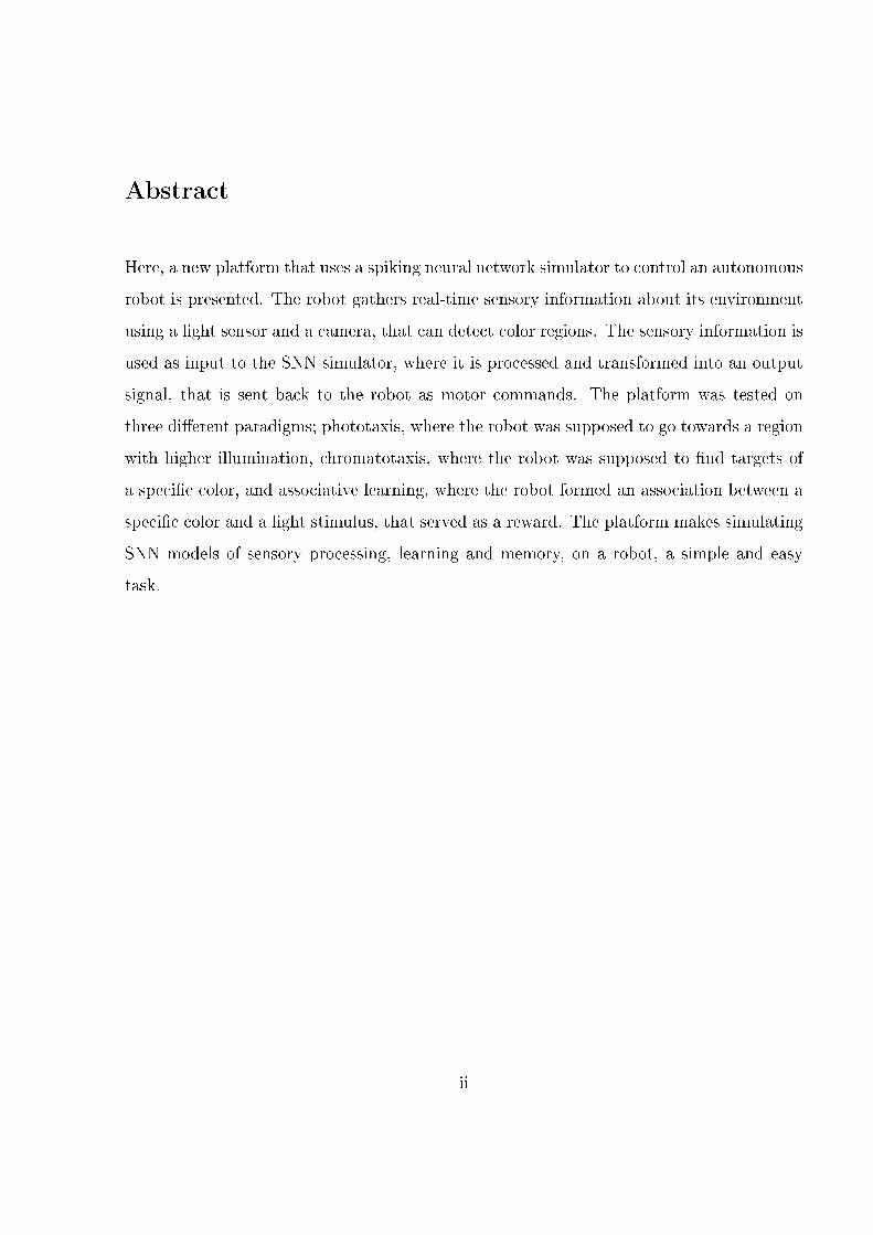
Here, a new platform that uses a spiking neural network simulator to control an autonomous

robot is presented. The robot gathers real-time sensory information about its environment

using a light sensor and a camera, that can detect color regions. The sensory information is

used as input to the SNN simulator, where it is processed and transformed into an output

signal, that is sent back to the robot as motor commands. The platform was tested on

three di�erent paradigms; phototaxis, where the robot was supposed to go towards a region

with higher illumination, chromatotaxis, where the robot was supposed to �nd targets of

a speci�c color, and associative learning, where the robot formed an association between a

speci�c color and a light stimulus, that served as a reward. The platform makes simulating

SNN models of sensory processing, learning and memory, on a robot, a simple and easy

task.

ii

Acknowledgements

I would like to thank Prof. Martin Nawrot, for giving me the opportunity to do this project.

Joachim Haenicke, for all the help, the endless discussions we had, also about the project,

and for reading over this manuscript. Hamid Moballegh for his help with the HaViMo

camera. Tim Landgraf for his input and enthusiasm. Fifa Finnsdottir for reading over the

manuscript.

Thanks to my family, especially my sisters, Ásta Guðrún, Rakel Björt, Margrét Ása and

my brother Heiðar Óli for their unconditional support and being greatest siblings in the

world.

Ásta Lovísa for being there for me and pressing buttons.

Saikat Ray, Hadi Roohani Rankoohi, Tiziano D'Albis, Helene Schmidt for all the times we

have shared and being my second family here in Berlin. To all my friends all over the world,

who have supported and believed in me.

I would also like to thank the professors and sta� of the BCCN for helping me get this close

to the �nishing line.

In the loving memory of Sigþór Bessi Bjarnason (1985-2011). I have been and always shall

be your friend.

Berlin, July 17th 2012


iii

List of Figures

1 Overview of the Drosophila Olfactory Learning Network . . . . . . . . . . . 4

2 iqr - SNN Simulator . . . . . . . . . . . . . . . . . . . . . . . . . . . . . . . 6

3 Arduino Duemilanove and Arduino IDE . . . . . . . . . . . . . . . . . . . . 9

4 DfRobotShop Rover . . . . . . . . . . . . . . . . . . . . . . . . . . . . . . . 11

5 HaViMo 2.0 . . . . . . . . . . . . . . . . . . . . . . . . . . . . . . . . . . . . 12

6 Overview of Platform . . . . . . . . . . . . . . . . . . . . . . . . . . . . . . . 15

7 Arena Measurements and Target Placement . . . . . . . . . . . . . . . . . . 18

8 Motor Function Network . . . . . . . . . . . . . . . . . . . . . . . . . . . . . 19

9 Raster Plots of the Pre-Motor Neuron Group . . . . . . . . . . . . . . . . . . 21

10 Robot Path: Phototaxis . . . . . . . . . . . . . . . . . . . . . . . . . . . . . 24

11 Robot Path: Chromatotaxis Blue Target . . . . . . . . . . . . . . . . . . . . 25

12 Robot Path: chromatotaxis Red Target . . . . . . . . . . . . . . . . . . . . . 26

13 Associative Learning Network . . . . . . . . . . . . . . . . . . . . . . . . . . 27

14 Screenshot: Association Raster and Connection Plots . . . . . . . . . . . . . 29

15 Robot Path: Associative Learning Color Red . . . . . . . . . . . . . . . . . 30

16 Robot Path: Associative Learning Color Blue . . . . . . . . . . . . . . . . . 30

iv

List of Tables

1 Features of Arduino Duemilanove . . . . . . . . . . . . . . . . . . . . . . . . 9

2 Common Arduino Functions . . . . . . . . . . . . . . . . . . . . . . . . . . . 10

3 moduleArduinoAnalog Input and Output Groups . . . . . . . . . . . . . . . 13

4 Details of Motor Function Network . . . . . . . . . . . . . . . . . . . . . . . 22

5 WiFi Con�guration for Ubuntu . . . . . . . . . . . . . . . . . . . . . . . . . 37

6 Socat Commands . . . . . . . . . . . . . . . . . . . . . . . . . . . . . . . . . 38

v

Contents

Preface i

Abstract . . . . . . . . . . . . . . . . . . . . . . . . . . . . . . . . . . . . . . . . . ii

Acknowledgements . . . . . . . . . . . . . . . . . . . . . . . . . . . . . . . . . . . iii

List of Figures . . . . . . . . . . . . . . . . . . . . . . . . . . . . . . . . . . . . . . iv

List of Tables . . . . . . . . . . . . . . . . . . . . . . . . . . . . . . . . . . . . . . v

Contents . . . . . . . . . . . . . . . . . . . . . . . . . . . . . . . . . . . . . . . . . vii

1 Introduction 1

1.1 Spiking Neural Networks . . . . . . . . . . . . . . . . . . . . . . . . . . . . . 2

1.2 Associative Learning . . . . . . . . . . . . . . . . . . . . . . . . . . . . . . . 3

1.3 Neurorobotics . . . . . . . . . . . . . . . . . . . . . . . . . . . . . . . . . . . 5

2 Platform Development 6

2.1 iqr - Spiking Neural Network Simulator . . . . . . . . . . . . . . . . . . . . 6

2.2 Arduino - A Robotic Platform . . . . . . . . . . . . . . . . . . . . . . . . . . 8

2.3 HaViMo - Vision Processing Module . . . . . . . . . . . . . . . . . . . . . . 12

2.4 Wireless Communication . . . . . . . . . . . . . . . . . . . . . . . . . . . . . 14

2.5 A Robotic Platform Controlled by a SNN Simulator . . . . . . . . . . . . . . 15

3 Test Cases 18

3.1 Phototaxis . . . . . . . . . . . . . . . . . . . . . . . . . . . . . . . . . . . . . 23

3.2 Chromatotaxis . . . . . . . . . . . . . . . . . . . . . . . . . . . . . . . . . . 24

3.3 Associative Learning . . . . . . . . . . . . . . . . . . . . . . . . . . . . . . . 26

4 Conclusions and Future Work 31

References 34

A Wireless Communication 35

A.1 Setting up the DfRobot WiFi Shield v. 2.1 for Arduino . . . . . . . . . . . . 35

A.2 WiFi Con�guration for Ubuntu . . . . . . . . . . . . . . . . . . . . . . . . . 37

vi

A.3 Socat Commands . . . . . . . . . . . . . . . . . . . . . . . . . . . . . . . . . 38

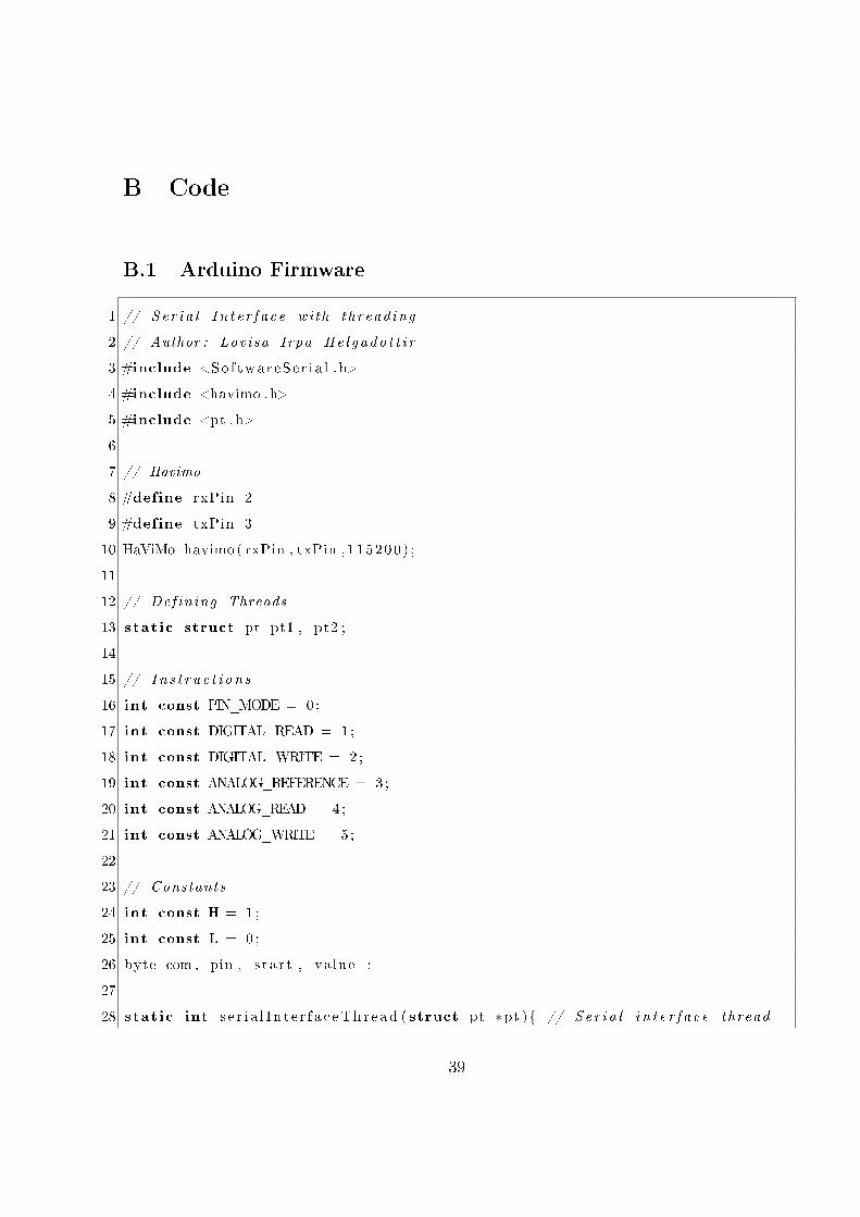
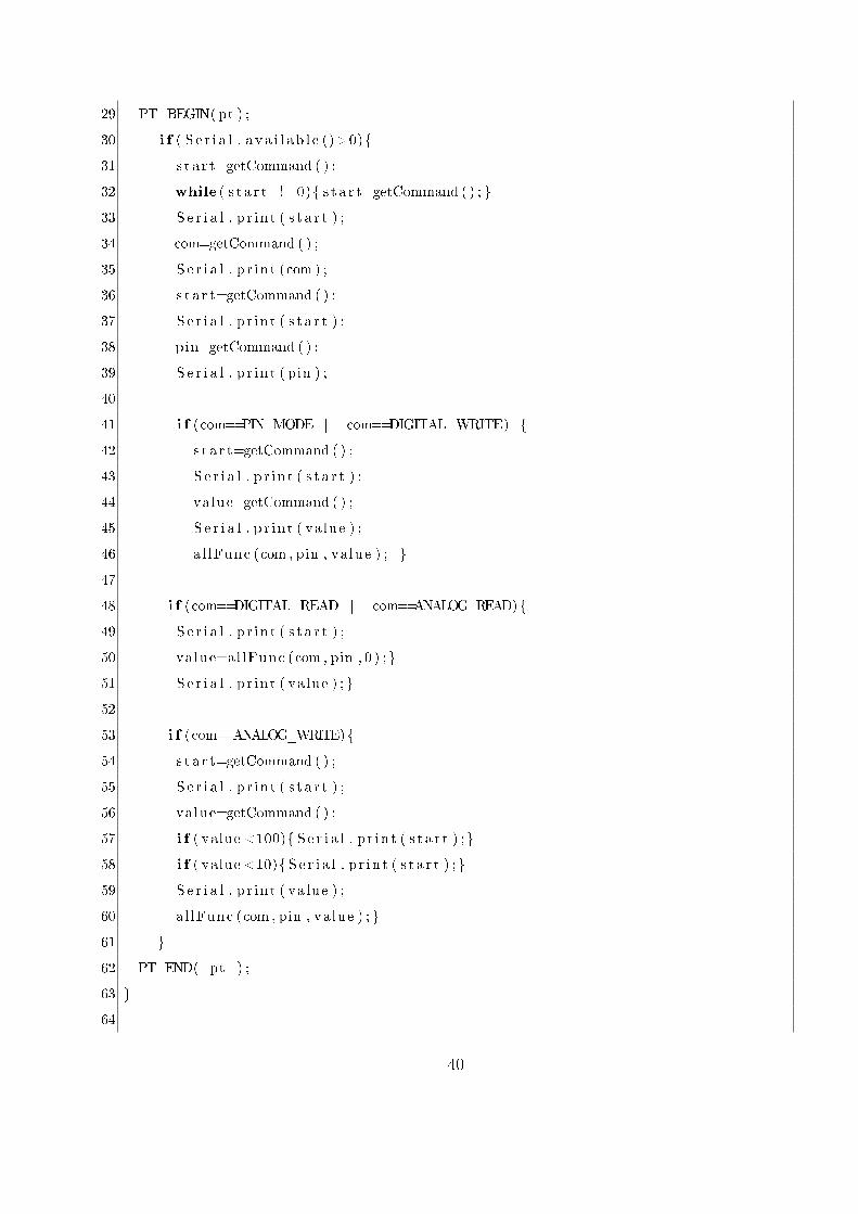
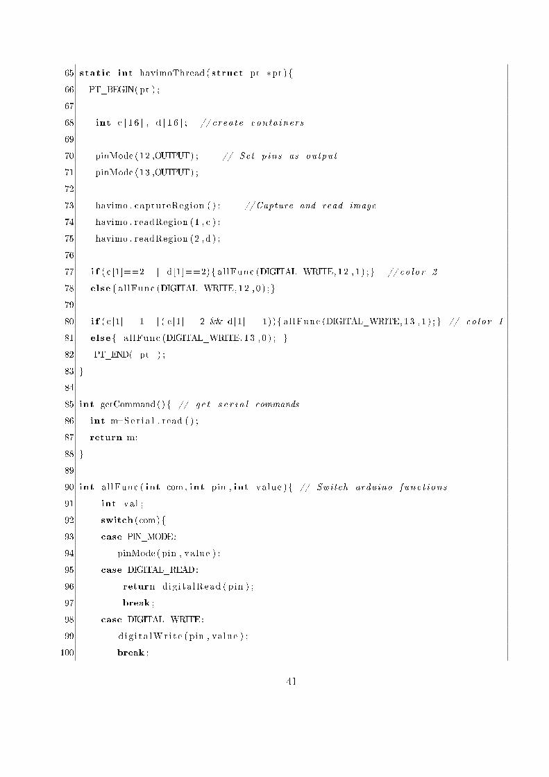
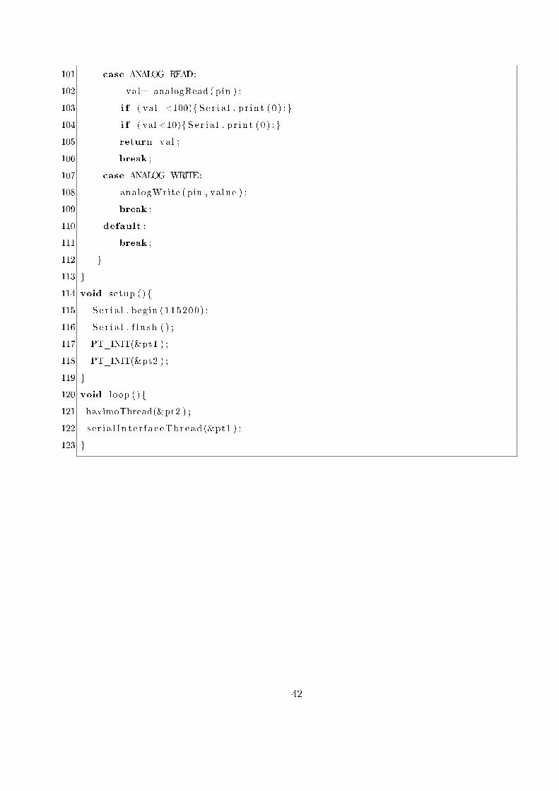
B Code 39

B.1 Arduino Firmware . . . . . . . . . . . . . . . . . . . . . . . . . . . . . . . . 39

B.2 HaViMo Library for Arduino . . . . . . . . . . . . . . . . . . . . . . . . . . . 43

vii

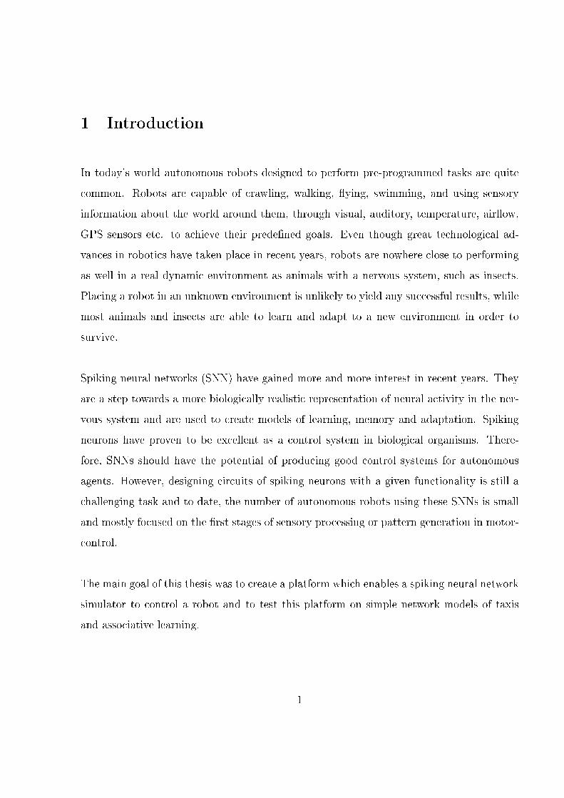
1 Introduction

In today's world autonomous robots designed to perform pre-programmed tasks are quite

common. Robots are capable of crawling, walking, �ying, swimming, and using sensory

information about the world around them, through visual, auditory, temperature, air�ow,

GPS sensors etc. to achieve their prede�ned goals. Even though great technological ad-

vances in robotics have taken place in recent years, robots are nowhere close to performing

as well in a real dynamic environment as animals with a nervous system, such as insects.

Placing a robot in an unknown environment is unlikely to yield any successful results, while

most animals and insects are able to learn and adapt to a new environment in order to

survive.

Spiking neural networks (SNN) have gained more and more interest in recent years. They

are a step towards a more biologically realistic representation of neural activity in the ner-

vous system and are used to create models of learning, memory and adaptation. Spiking

neurons have proven to be excellent as a control system in biological organisms. There-

fore, SNNs should have the potential of producing good control systems for autonomous

agents. However, designing circuits of spiking neurons with a given functionality is still a

challenging task and to date, the number of autonomous robots using these SNNs is small

and mostly focused on the �rst stages of sensory processing or pattern generation in motor-

control.

The main goal of this thesis was to create a platform which enables a spiking neural network

simulator to control a robot and to test this platform on simple network models of taxis

and associative learning.

1

1.1 Spiking Neural Networks

Nervous systems convey information through action potential (spikes). A spike travels

along the axon of a neuron until it reaches the cells' synapses. There, a neurotransmitter is

released into the extracellular body and reaches the matching receptors of the post-synaptic

neuron. This triggers a post-synaptic potential that can either have an excitatory or an

inhibitory e�ect on the post-synaptic neuron [7].

SNNs are a way of modelling these neurons in a biologically realistic way. Unlike other

Arti�cial Neural Network (ANN) that use rate-coding, i.e. higher rates of �ring correlate

with higher output, SNNs use pulse coding or temporal coding where spike timing is the

important aspect of information processing [7] [18]. SNNs have been shown be computa-

tionally more powerful than the classical ANNs [11] and more robust, since noise and failure

of individual elements (neurons or synapses) do not disrupt the network function [18]. They

should be ideal for robotic control, allowing robots to perform tasks with minimal knowl-

edge about the environment. However, implementing SNNs onto hardware is not an easy

task, and still the number of robots using SNNs is low.

Adaptive Intergrate-And-Fire Neurons

The best known model of spiking neurons is the integrate-and-�re neuron (IFN). It is based

on a simple principle of electronics, where the neuron acts as a low pass �lter, i.e. a circuit

with a resistor and a capacitor in parallel and is described by

τmdV

dt= EL − V +RmIe, (1)

where V is the membrane potential, EL is the reversal potential, τm is the membrane time

constant, Rm is the membrane resistance and Ie is the stimulating current. To generate

spikes, the membrane potential V must reach a predetermined threshold Vth. Then a spike

is �red and the membrane potential is reset. When a constant current is injected into

the neuron, most real-neurons exhibit spike-rate adaptation, i.e. the inter-spike interval

2

lengthens with time, before settling to a steady state value. By including an additional

current into the model described in equation (1) we can add the spike-rate adaptation to

the model,

τmdV

dt= EL − V − rmgsra(V − Esra) +RmIe. (2)

Here, gsra is the spike-rate adaptation conductance that increases with every spike the

neuron �res, introducing a current that drives the membrane potential towards the reversal

potential Esra, causing the �ring rate to adapt. When no spikes are �red, the conductance

decreases exponentially to 0. rm is the speci�c membrane resistance [7]. This model is

very simple and can easily be implemented in neuromorphic hardware which allows the

implementation of large networks of spiking neurons in small, light-weighted and low-power

chips [18] [9].

1.2 Associative Learning

Most animals have the ability to associate a reward or punishment with a stimulus and to

learn the proper action in response. This process of learning is called associative learning

and is typically tested in paradigms of classical conditioning and operand conditioning.

In classical conditioning schemes a response to a stimulus is reinforced until the stimulus

itself can elicit the response without the reinforcement. In operand conditioning actions

of the animals determine the way reinforcements are administered, which in�uences the

probability of actions being repeated [7]. An example of a well studied associative learning

paradigm using classical conditioning is the proboscis extension response of honeybees to

olfactory stimuli paired with a sugar reward [4] [16].

A Model of the Olfactory Learning in Insects

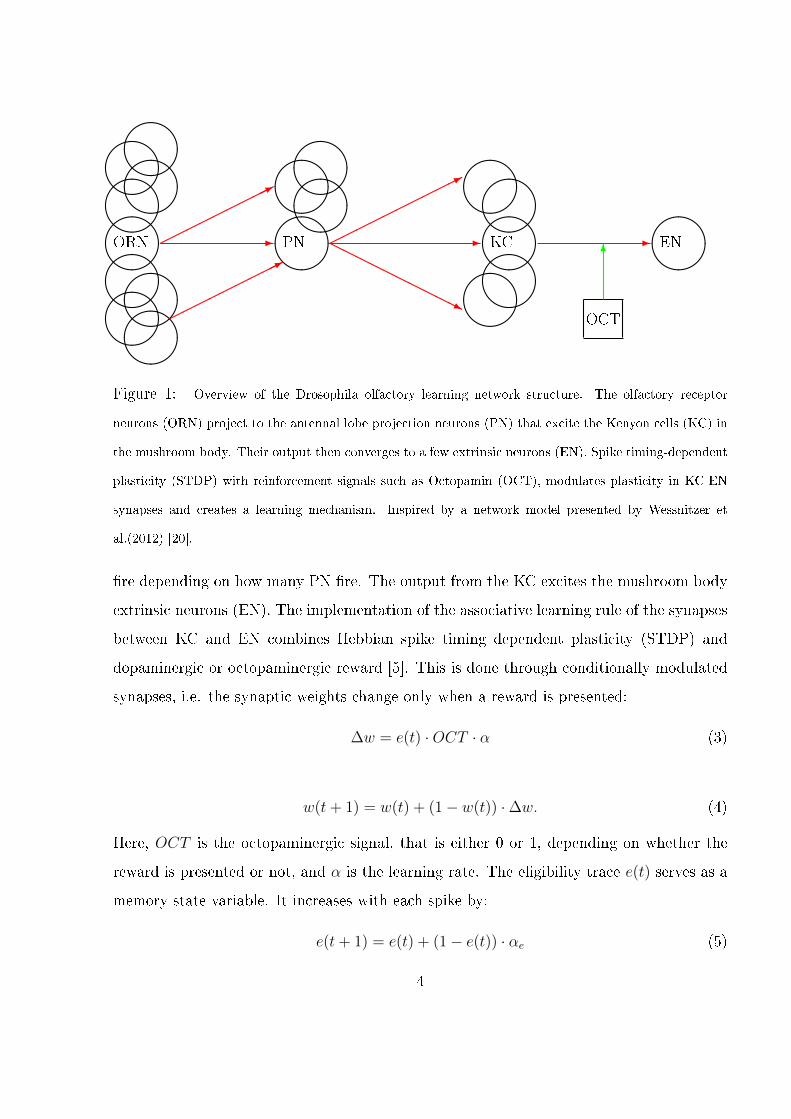
Figure 1 shows a network model of olfactory learning in Drosophila [20]. Odours are detected

by the olfactory receptor neurons (ORN), and when stimulated they project the input to

the antennal lobe projection neurons (PN). The PN excite the mushroom body intrinsic

neurons, the Kenyon cells (KC). The KC supposedly serve as a coincident detector and will

3

&%'$

&%'$

&%'$

&%'$&%'$&%'$

&%'$

&%'$

&%'$

ORN &%'$&%

'$&%'$

&%'$

PN

&%'$

&%'$&%'$&%'$

&%'$

KC &%'$EN

OCT

��

��*

-

��

��

��*

��

��

��*

HHHHHH

HHHHj

- -6

Figure 1: Overview of the Drosophila olfactory learning network structure. The olfactory receptor

neurons (ORN) project to the antennal lobe projection neurons (PN) that excite the Kenyon cells (KC) in

the mushroom body. Their output then converges to a few extrinsic neurons (EN). Spike timing-dependent

plasticity (STDP) with reinforcement signals such as Octopamin (OCT), modulates plasticity in KC-EN

synapses and creates a learning mechanism. Inspired by a network model presented by Wessnitzer et

al.(2012) [20].

�re depending on how many PN �re. The output from the KC excites the mushroom body

extrinsic neurons (EN). The implementation of the associative learning rule of the synapses

between KC and EN combines Hebbian spike timing dependent plasticity (STDP) and

dopaminergic or octopaminergic reward [5]. This is done through conditionally modulated

synapses, i.e. the synaptic weights change only when a reward is presented:

∆w = e(t) ·OCT · α (3)

w(t+ 1) = w(t) + (1− w(t)) ·∆w. (4)

Here, OCT is the octopaminergic signal, that is either 0 or 1, depending on whether the

reward is presented or not, and α is the learning rate. The eligibility trace e(t) serves as a

memory state variable. It increases with each spike by:

e(t+ 1) = e(t) + (1− e(t)) · αe (5)

4

but decreases exponentially when no spikes are �red:

e(t+ 1) = e(t) · exp(−∆t

τe). (6)

The eligibility increases with each spike by αe, and τe is the eligibility time constant, which

determines how fast it decreases when no spikes are �red.

1.3 Neurorobotics

Neurorobots are robotic devices that are equipped with control systems based on principles

of nervous systems. They are used as a tool for modelling and simulating neuronal function

and behaviour in a real environment. Neurorobots can help us in understanding questions

pertaining to neuroscience, unlike biologically inspired robotics, which draws inspiration

from biology to improve robotic technology [10].

Neurorobots using SNN are few and mainly focus on primary sensory processing or simple

motor control. Although a lot of research and simulations of SNN paradigms that could be

tested in robotics have been done [17], implementing and testing these paradigms has in

many cases not been done due to many limiting factors. One is the lack of a simple interface

between SNN simulators and robotic platforms. Another is the lack of inexpensive robotic

platforms for neurorobotic research.

Custom made neurorobots, like theWhiskerbot and SCRATCHbot [13], use reprogrammable

Field Programmable Gate Arrays (FPGA) to run detailed spiking neural networks on-

board the robot. Webbs' cricket robot [19] uses a leaky-integrate-and-�re neural model

of phonotaxis in crickets. It has an analogue electronic auditory system that converts an

auditory input into spikes, that are fed into a SNN simulator. It is important to point

out that no learning is implemented on-board the aforementioned robots. In 2009 Cox and

Krichmar presented a robot control using neuromodulation inspired by the mammalian

brain [6]. However, they used a mean �ring rate neural model instead of a spiking neural

model.

5

2 Platform Development

In this section a platform is presented, which uses a SNN simulator to control a small

tracked robot. The robot is equipped with a camera, a light sensor and a temperature

sensor that are used to gather real time sensory information about the environment. The

sensory input is then sent via WiFi to the SNN, which processes it and sends it output to

the motors of the robot. The platform is inexpensive yet versatile as well as simple and

easy to set up and use.

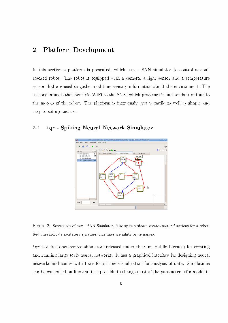
2.1 iqr - Spiking Neural Network Simulator

Figure 2: Screenshot of iqr - SNN Simulator. The system shown creates motor functions for a robot.

Red lines indicate excitatory synapses, blue lines are inhibitory synapses.

iqr is a free open-source simulator (released under the Gnu Public Licence) for creating

and running large scale neural networks. It has a graphical interface for designing neural

networks and comes with tools for on-line visualization for analysis of data. Simulations

can be controlled on-line and it is possible to change most of the parameters of a model in

6

run-time. Most importantly, for the purpose of this project, it has an open architecture,

which makes extensions for our needs possible. We can therefore write our own models for

neurons and synapses and create interfaces to real world hardware like robots and sensors.

Models in iqr are organized into di�erent levels. Top level is the system, which contains an

arbitrary number of processes and connections between processes. Each process consists of

an arbitrary number of groups. Each group consists of neurons of identical type arranged

in a speci�c topology. Connections between groups are de�ned as a collection of synapses

of identical type. The connecting synapses can be excitatory, inhibitory or modulatory

and their connectivity is comprised of how the pattern and the arborization are de�ned.

The pattern de�nes pairs of points in the lattice of the pre- and post-synaptic group. The

arborization determines whether the connection is formed as a receptive �eld or a projective

�eld and is applied to every pair of points de�ned by the pattern [3].

Conditional Plasticity

One of the goals of this project was to implement a model of conditional plasticity in in-

sects (see chapter 1.2) and integrate it onto the robotic platform, so its principles could

be used in a associative learning paradigm. The model required the adaptive IFN model

as describe in equation 2 and modulatory synapses based on the Hebbian learning rule as

described in equations 3 and 4. Because the adaptive IFN had already been implemented in

iqr by the former group member Jan Meyer [12], it was only necessary to add a modulatory

feedback parameter to the neuron module. The design of iqr requires the reinforcement

to be directly applied to a neuron group via modulatory connections. The information is

stored as a parameter that can be accessed by synapses that are supposed to be modulated.

The modulatory connection from the reinforcement to the neuron group is not the same as

the synapses that will be modulated and it has no e�ect on the output of the connected

neuron group. The synapses that will be modulated can either be excitatory or inhibitory,

but they do not a�ect the neuron group until after reinforcement is applied.

7

A synapse module whose weights could be modulated with a reinforcement input during

simulation had not been implemented in iqr before. The synapseModulateFeedback mod-

ule was created for this purpose. During a simulation, the modulatory feedback from each

neuron group is read in every cycle. Before the reinforcement is administered the synapses

show no activity for any stimulus. Any pre-synaptic activity is integrated into the eligi-

bility trace as described in equations 5 and 6. During reinforcement the variable OCT is

changed from 0 to 1. If the reinforcement occurs when the pre-synaptic activity is non-zero

the weights are changed as described by equation 3. Once a certain stimulus has been

reinforced, the synapses will excite or inhibit the post-synaptic neuron group every time

the reinforced stimulus is presented but will be quiet for all other stimuli.

2.2 Arduino - A Robotic Platform

Arduino is an inexpensive open source microcontroller board, designed to make the use of

electronics easy and accessible to all. A large community of users exists and the community

is well supported. Many o�cial and non-o�cial accessories and shields are available making

it an exciting board to work with.

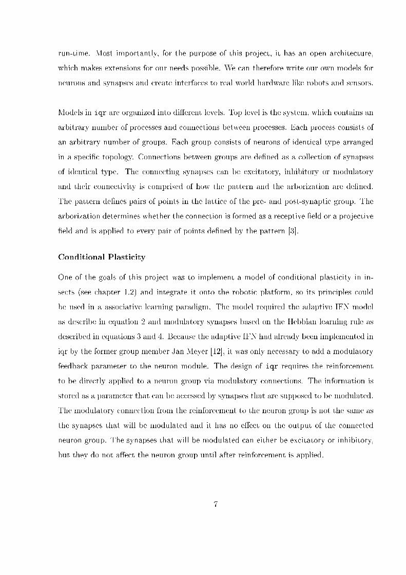
Arduino Duemilanove

The microcontroller board used is the Arduino Duemilanove board. It features a AT-

Mega328p microcontroller, 14 digital I/O pins, six analog inputs, a USB connection and a

power jack. Six of the digital I/O pins can provide a 8-bit PWM output (pins 3,5,6,9,10,11).

The Arduino Duemilanove provides serial communication which is available on digital pins

0 (Rx) and 1 (Tx). The FTDI FT232RL chip on the board channels this serial communica-

tion over the USB connection to a PC. A DfRobot WiFi Shield v. 2.1 for Arduino was used

for wireless serial communication between the board and the PC. The library SoftwareSerial

was used for communicate serially with devices attached to the digital pins of the Arduino

Duemilanove board [2]. A summary of the features of the Arduino Duemilanove is given in

table 1.

8

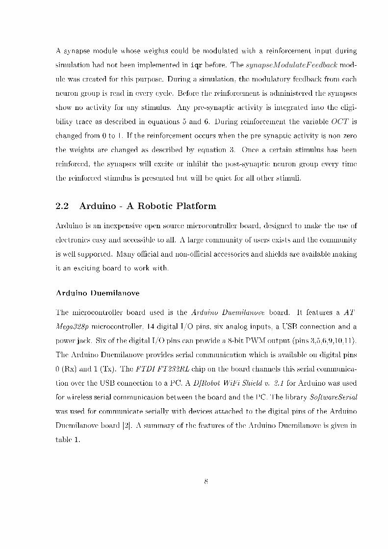
(A) (B)

Figure 3: (A) The Arduino Duemilanove microcontroller board, (B) Screenshot of Arduino IDE that

shows an example of a sketch that makes a diode blink.

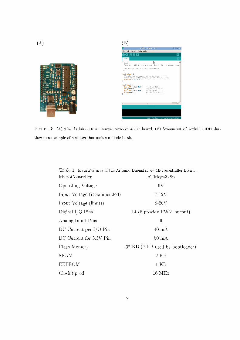
Table 1: Main Features of the Arduino Duemilanove Microcontroller Board

MicroController ATMega328p

Operating Voltage 5V

Input Voltage (recommended) 7-12V

Input Voltage (limits) 6-20V

Digital I/O Pins 14 (6 provide PWM output)

Analog Input Pins 6

DC Current per I/O Pin 40 mA

DC Current for 3.3V Pin 50 mA

Flash Memory 32 KB (2 KB used by bootloader)

SRAM 2 KB

EEPROM 1 KB

Clock Speed 16 MHz

9

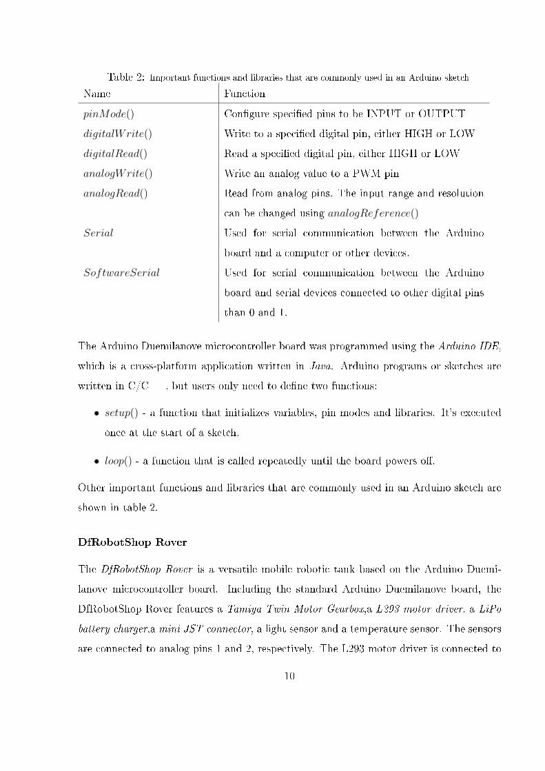
Table 2: Important functions and libraries that are commonly used in an Arduino sketch

Name Function

pinMode() Con�gure speci�ed pins to be INPUT or OUTPUT

digitalWrite() Write to a speci�ed digital pin, either HIGH or LOW

digitalRead() Read a speci�ed digital pin, either HIGH or LOW

analogWrite() Write an analog value to a PWM pin

analogRead() Read from analog pins. The input range and resolution

can be changed using analogReference()

Serial Used for serial communication between the Arduino

board and a computer or other devices.

SoftwareSerial Used for serial communication between the Arduino

board and serial devices connected to other digital pins

than 0 and 1.

The Arduino Duemilanove microcontroller board was programmed using the Arduino IDE,

which is a cross-platform application written in Java. Arduino programs or sketches are

written in C/C++, but users only need to de�ne two functions:

• setup() - a function that initializes variables, pin modes and libraries. It's executed

once at the start of a sketch.

• loop() - a function that is called repeatedly until the board powers o�.

Other important functions and libraries that are commonly used in an Arduino sketch are

shown in table 2.

DfRobotShop Rover

The DfRobotShop Rover is a versatile mobile robotic tank based on the Arduino Duemi-

lanove microcontroller board. Including the standard Arduino Duemilanove board, the

DfRobotShop Rover features a Tamiya Twin Motor Gearbox,a L293 motor driver, a LiPo

battery charger,a mini JST connector, a light sensor and a temperature sensor. The sensors

are connected to analog pins 1 and 2, respectively. The L293 motor driver is connected to

10

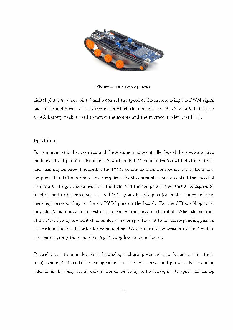
Figure 4: DfRobotShop Rover

digital pins 5-8, where pins 5 and 6 control the speed of the motors using the PWM signal

and pins 7 and 8 control the direction in which the motors turn. A 3.7 V LiPo battery or

a 4AA battery pack is used to power the motors and the microcontroller board [15].

iqr-duino

For communication between iqr and the Arduino microcontroller board there exists an iqr

module called iqr-duino. Prior to this work, only I/O communication with digital outputs

had been implemented but neither the PWM communication nor reading values from ana-

log pins. The DfRobotShop Rover requires PWM communication to control the speed of

its motors. To get the values from the light and the temperature sensors a analogRead()

function had to be implemented. A PWM group has six pins (or in the context of iqr,

neurons) corresponding to the six PWM pins on the board. For the dfRobotShop rover

only pins 5 and 6 need to be activated to control the speed of the robot. When the neurons

of the PWM group are excited an analog value or speed is sent to the corresponding pins on

the Arduino board. In order for commanding PWM values to be written to the Arduino,

the neuron group Command Analog Writing has to be activated.

To read values from analog pins, the analog read group was created. It has two pins (neu-

rons), where pin 1 reads the analog value from the light sensor and pin 2 reads the analog

value from the temperature sensor. For either group to be active, i.e. to spike, the analog

11

values need to cross a prede�ned threshold.

The moduleArduinoAnalog consists of six input groups and two output groups. The topol-

ogy of neuron groups Digital Read and Digital Write are de�ned so that each process has

twelve neurons corresponding to the twelve digital pins on the Arduino board. The pins 0

and 1 are not used as they are busy with the serial communication between the iqr and

the Arduino board. Table 3 describes the groups and their function.

2.3 HaViMo - Vision Processing Module

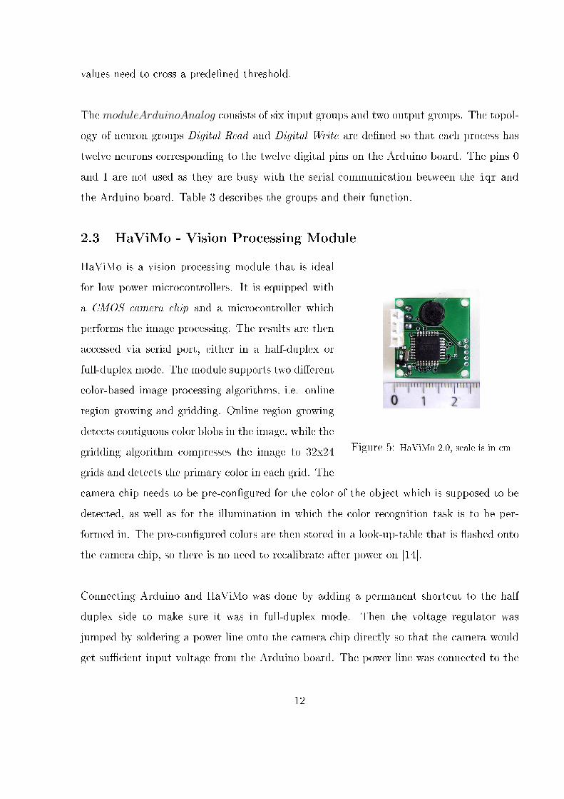
Figure 5: HaViMo 2.0, scale is in cm

HaViMo is a vision processing module that is ideal

for low power microcontrollers. It is equipped with

a CMOS camera chip and a microcontroller which

performs the image processing. The results are then

accessed via serial port, either in a half-duplex or

full-duplex mode. The module supports two di�erent

color-based image processing algorithms, i.e. online

region growing and gridding. Online region growing

detects contiguous color blobs in the image, while the

gridding algorithm compresses the image to 32x24

grids and detects the primary color in each grid. The

camera chip needs to be pre-con�gured for the color of the object which is supposed to be

detected, as well as for the illumination in which the color recognition task is to be per-

formed in. The pre-con�gured colors are then stored in a look-up-table that is �ashed onto

the camera chip, so there is no need to recalibrate after power on [14].

Connecting Arduino and HaViMo was done by adding a permanent shortcut to the half

duplex side to make sure it was in full-duplex mode. Then the voltage regulator was

jumped by soldering a power line onto the camera chip directly so that the camera would

get su�cient input voltage from the Arduino board. The power line was connected to the

12

Table 3: The moduleArduinoAnalog input and output groups and their functionality

Output groups

Command Digital Writing Send a value di�erent than 0 to the cell assigned to the

pin which are supposed to be accessed.

Command Digital Reading Send a value di�erent than 0 to each of its 12 cells in

order to command a digital reading of its assigned pin

(�rst cell belongs to pin 2; last one to pin 13).

Digital writing Once writing is commanded, this group manipulates the

output value.

Command Analog Writing Send a value di�erent than 0 to the cell assigned to the

pin which you want to access in PWK mode.

Analog Writing Once writing is commanded, this group manipulates the

output value.

Command Analog Reading Send a value di�erent than 0 to each of its 2 cells in order

to command an analog reading of its assigned pin (cell

1 belongs to the light sensor; cell 2 to the temperature

sensor ).

Input groups

Digital Reading Once reading is commanded, the input value will be pre-

sented as activity in this group.

Analog Reading Once analog reading is commanded, the input values

over threshold de�ned by the light sensitivity parameter

will be presented as activity in this group.

13

5V pin on the Arduino board and the ground of the camera was connected to the GND pin.

The Rx and the Tx of the camera were connected to digital pins 2 and 3 on the Arduino

board, de�ned as Tx and Rx, respectively. To make the HaViMo interact with the Arduino,

I created a library havimo for Arduino (Appendix B.2), that uses the SoftwareSerial library,

and implements all the basic commands easily. The function captureRegion() is called to

capture the image and to �nd regions within the image containing the precon�gured color.

These regions are then stored on the camera chip in the address range 0x10 to 0xFF and

can be read with the command readRegion() .

2.4 Wireless Communication

Communication between iqr and the Arduino board is done via wireless connection. A

DfRobot WiFi shield v. 2.1 for Arduino is used. How to set up the WiFi shield is described

in appendix A.1. Once the connection between a workstation and the Arduino board has

been established, it is easy to communicate with the Arduino, e.g. through a terminal

using netcat, depending on the sketch running. The Arduino board reads the data from

the computer with Serial.read() and sends out data using Serial.write() or Serial.print(),

one byte at a time. The con�guration for the wireless connection between the Arduino and

a PC running linux OS (i.e. Ubuntu 10.04) are described in appendix A.2.

Virtual Serial Port

Serial communication between Arduino sketches and iqr is quite simple. Therefore, a

virtual serial port is created through which the communication between the Arduino board

and iqr takes place, using the program utility socat. Socat is a command-line based utility

that establishes two bidirectional byte streams and transfers data between them [1]. To

establish a stable communication the following command is run:

socat -d -d -d -x -s -t 30 TCP4:192.181.10.100:4000,reuseaddr

PTY,raw,ispeed=115200,ospeed=115200,echo=0,onlcr=0,iexten=0,echoctl=0,

echoke=0,sane

14

This creates a virtual serial port on the workstation, e.g. /dev/pts/0 in Ubuntu. Further

details of the virtual serial port are in appendix A.3.

2.5 A Robotic Platform Controlled by a SNN Simulator

?

6

RX/TXVirtual SerialPort\dev\pts\2

��

��

��

WiFi

(TCP)

HHHHH

HYHH

HHHHjSerial

comm.

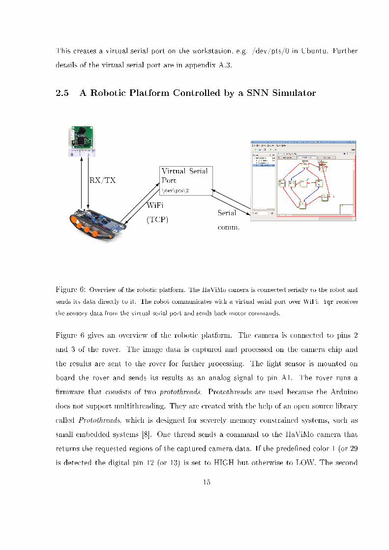
Figure 6: Overview of the robotic platform. The HaViMo camera is connected serially to the robot and

sends its data directly to it. The robot communicates with a virtual serial port over WiFi. iqr receives

the sensory data from the virtual serial port and sends back motor commands.

Figure 6 gives an overview of the robotic platform. The camera is connected to pins 2

and 3 of the rover. The image data is captured and processed on the camera chip and

the results are sent to the rover for further processing. The light sensor is mounted on

board the rover and sends its results as an analog signal to pin A1. The rover runs a

�rmware that consists of two protothreads. Protothreads are used because the Arduino

does not support multithreading. They are created with the help of an open source library

called Protothreads, which is designed for severely memory constrained systems, such as

small embedded systems [8]. One thread sends a command to the HaViMo camera that

returns the requested regions of the captured camera data. If the prede�ned color 1 (or 29

is detected the digital pin 12 (or 13) is set to HIGH but otherwise to LOW. The second

15

thread receives commands serially from iqr over the virtual serial port and sends back the

proper response, e.g. reading the status of a pin (either digital or analog) or writing to a

pin (either 1 or 0 or a PWM signal). The data is fed to the SNN being simulated in iqr

over the wireless connection, and the output of the network is sent back to the robot as

motor control commands, i.e. Analog Writing to pins 5 and 6.

Before starting a simulation, a few steps need to be taken. Once the robot has been turned

on, it is advisable to see whether the protothreads are working correctly and whether the

camera has booted up in the right mode. A LED can be mounted to pin 12 (or 13) to

get visual feedback on whether the HaViMo thread is running, and if it is detecting the

color de�ned as color 1 (or 2). If the LED blinks the thread is working correctly. Then

the virtual serial port is created on the workstation using socat in a terminal (see chapter

2.4). This will make the LED stop blinking, since now the second protothread is waiting

for input, which it will not receive until the iqr simulation starts.

Adding the Arduino process to the SNN is done graphically in iqr. First the module Ar-

duinoAnalog is selected, and it consists of eight groups as described in table 3. Even though

not all groups will be used during a simulation, they must all be in place. However, there is

no need to activate the unused groups. The serial device selected has to be the virtual serial

port that was created (eg. /dev/pts/2). The parameters Analog Write, which controls the

speed of the robot, and light sensitivity, which controls the threshold of illumination, must

be set to appropriate values.

The output from the group Digital Reading and/or the group Analog Reading can be used

as a sensory input to the network, depending on whether the sensory input is supposed to be

light and/or camera data. Before it is possible to read sensory data, the groups Command

Digital Reading and Command Analog Reading must be activated for the corresponding

pins. The output of the network should be sent to pins 5 to 8, where the speed is controlled

by the group Analog Writing that must write to pins 5 and 6. The rotation is controlled by

the group Digital Writing that writes to pins 7 and 8. LOW is clockwise, HIGH is counter-

16

clockwise. In the current implementation the speed must be set before the simulation starts.

It must be in the range between 0 and 255, and can only be changed manually during the

simulation. If the rotation of the motors of the robot are supposed to be the output, the

speed must also be activated. Otherwise the robot does not turn the motors. The output

of the SNN is only sent to the robot if the groups Command Digital Writing and Command

Analog Writing are activated.

Limits

There are some limitations to the platform, that in�uence its performance. The number of

synapses and the amount of spikes being propagated through the network determine the

maximum network size for real-time simulation. Based on the employed network structure,

this limit was around 10000 neurons and connections, as the simulations were supposed to

run at 1000 cycles per second (Intel i7, 2.50 GHz).

The HaViMo camera needs about 300 - 500 ms to capture, process and send the data. This

results in a delay for the sensory data to reach the network, which has an e�ect on the

network performance, that accumulates over time.

Another issue is the power. LiPo batteries do not supply enough current to run the motors,

so the rover moves painfully slowly if they are used. It is also possible to use a 4 AA

battery pack to power the rover. However, they can only power either the motors or the

microcontroller board, but not both at the same time. A temporary solution to this problem

was to power the motors and the microcontroller board separately, powering the motor with

the 4 AA battery pack and the microcontroller board through the USB connector.

17

3 Test Cases

To demonstrate the ability of the robotic platform three di�erent networks were tested;

phototaxis (3.1), where the on-board light sensor was used as sensory input, chromatotaxis

(3.2), where the camera data was used, and associative learning (3.3), where the light sen-

sor, the camera and modulating synapses were combined to perform a simple associative

learning task.

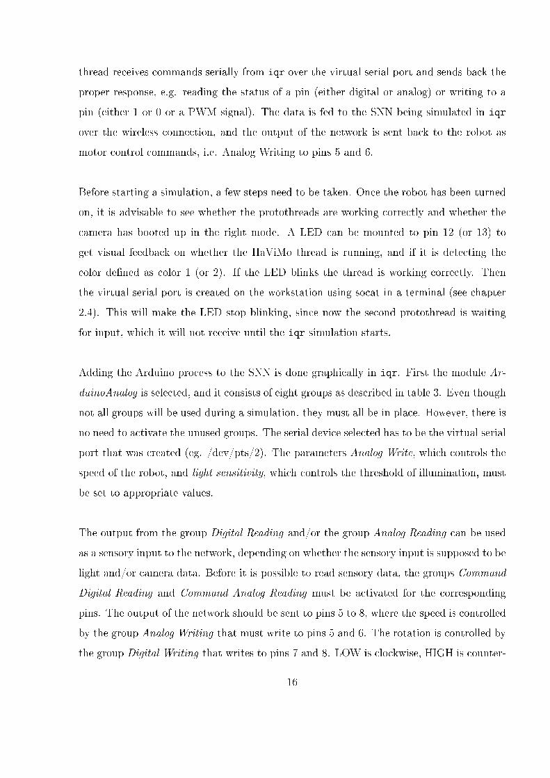
(A)

start

Target

Target

107cm

110cm

55cm

57cm

(B)

Target Target

107cm

110cm

55cm

57cm

Figure 7: Arena measurements and placements of targets. (A) The yellow borders indicate where the

light concentration was above light sensitivity threshold (for phototaxis). The blue and the red targets

were used for the chromatotaxis paradigm. (B) The blue and red lines indicate the placement of targets

for the associative learning test case. As a reward an additional light source was placed near either one of

the target (yellow line).

A small arena was used for testing the robotic platform. The robot was positioned in the

middle of the arena. When the simulation started, it explored the arena looking for its

18

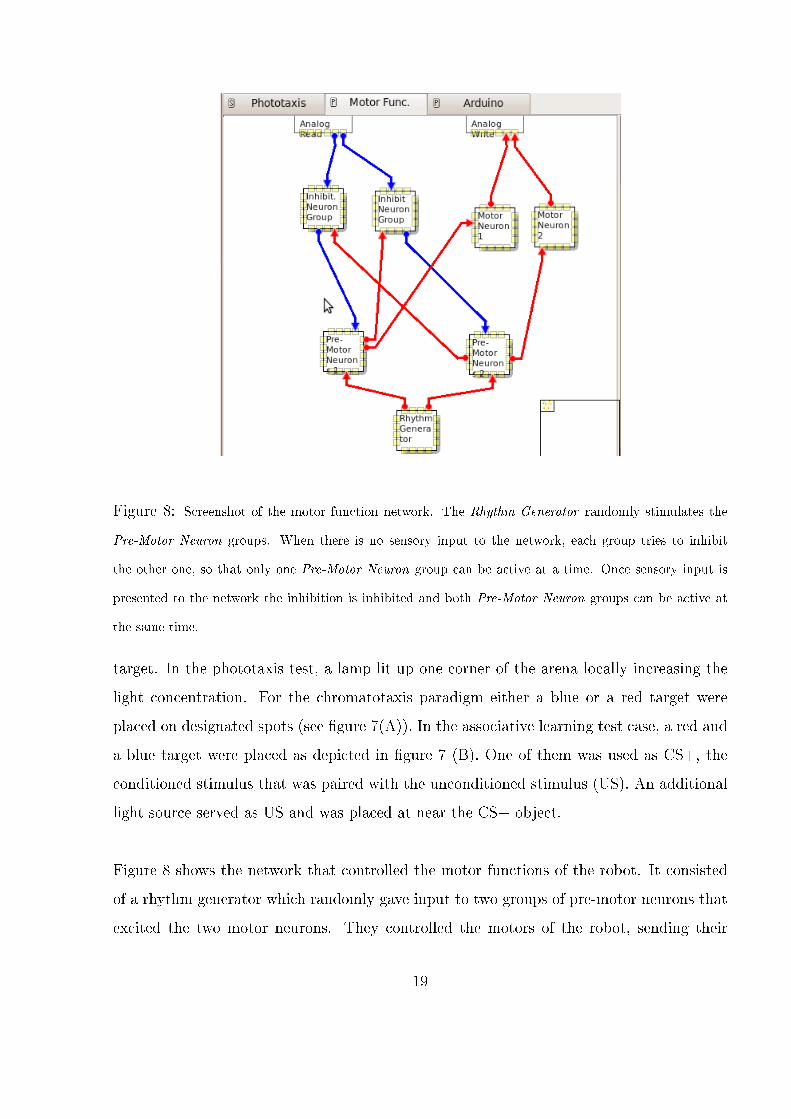
Figure 8: Screenshot of the motor function network. The Rhythm Generator randomly stimulates the

Pre-Motor Neuron groups. When there is no sensory input to the network, each group tries to inhibit

the other one, so that only one Pre-Motor Neuron group can be active at a time. Once sensory input is

presented to the network the inhibition is inhibited and both Pre-Motor Neuron groups can be active at

the same time.

target. In the phototaxis test, a lamp lit up one corner of the arena locally increasing the

light concentration. For the chromatotaxis paradigm either a blue or a red target were

placed on designated spots (see �gure 7(A)). In the associative learning test case, a red and

a blue target were placed as depicted in �gure 7 (B). One of them was used as CS+, the

conditioned stimulus that was paired with the unconditioned stimulus (US). An additional

light source served as US and was placed at near the CS+ object.

Figure 8 shows the network that controlled the motor functions of the robot. It consisted

of a rhythm generator which randomly gave input to two groups of pre-motor neurons that

excited the two motor neurons. They controlled the motors of the robot, sending their

19

output as a PWM signal to pins 5 and 6 on the robot. These two groups of pre-motor

neurons competed for dominance by inhibiting each other so only one group of neurons was

active at a time. This made the robot move and turn either to the right or to the left for

random time intervals, in the order of seconds, throughout the trial. As a consequence the

robot explored the arena. When sensory input was fed to the network the inhibitory neuron

groups of the two pre-motor neurons are inhibited. This lead to both pre-motor neuron

groups being constantly active and the robot moves straight forward towards its target.

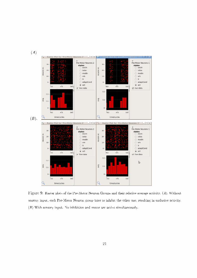
The network performed at 1000 cycles per second and the total number of neurons was

293 and total number of connections was 7922 . Numerical details of the motor function

network are in table 4.

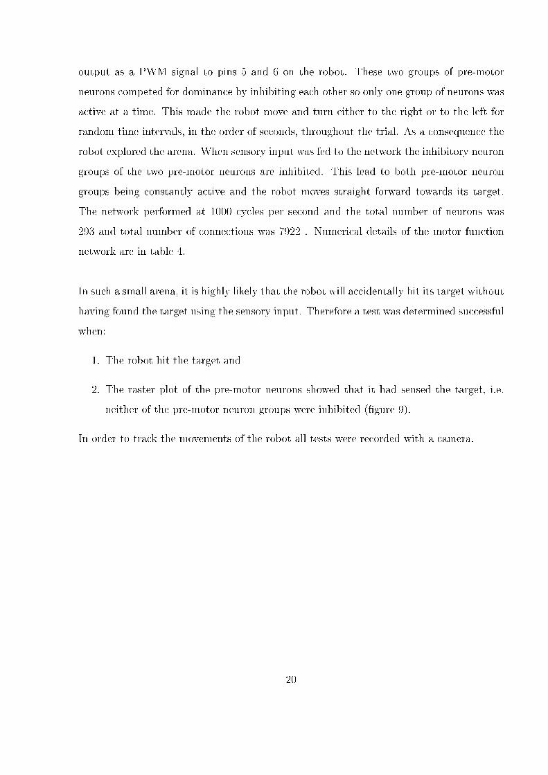
In such a small arena, it is highly likely that the robot will accidentally hit its target without

having found the target using the sensory input. Therefore a test was determined successful

when:

1. The robot hit the target and

2. The raster plot of the pre-motor neurons showed that it had sensed the target, i.e.

neither of the pre-motor neuron groups were inhibited (�gure 9).

In order to track the movements of the robot all tests were recorded with a camera.

20

(A)

(B).

Figure 9: Raster plots of the Pre-Motor Neuron Groups and their relative average activity. (A). Without

sensory input, each Pre-Motor Neuron group tries to inhibit the other one, resulting in exclusive activity.

(B) With sensory input. No inhibition and motor are active simultaneously.

21

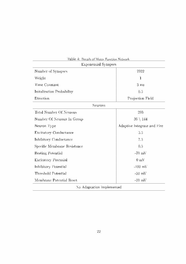
Table 4: Details of Motor Function Network

Exponential Synapses

Number of Synapses 7922

Weight 1

Time Constant 3 ms

Initalization Probability 0.5

Direction Projection Field

Neurons

Total Number Of Neurons 293

Number Of Neurons In Group 36 \ 144

Neuron Type Adaptive Integrate and Fire

Excitatory Conductance 5.5

Inhibitory Conductance 7.5

Speci�c Membrane Resistance 0.5

Resting Potential -70 mV

Excitatory Potential 0 mV

Inhibitory Potential -100 mV

Threshold Potential -50 mV

Membrane Potential Reset -70 mV

No Adaptation implemented

22

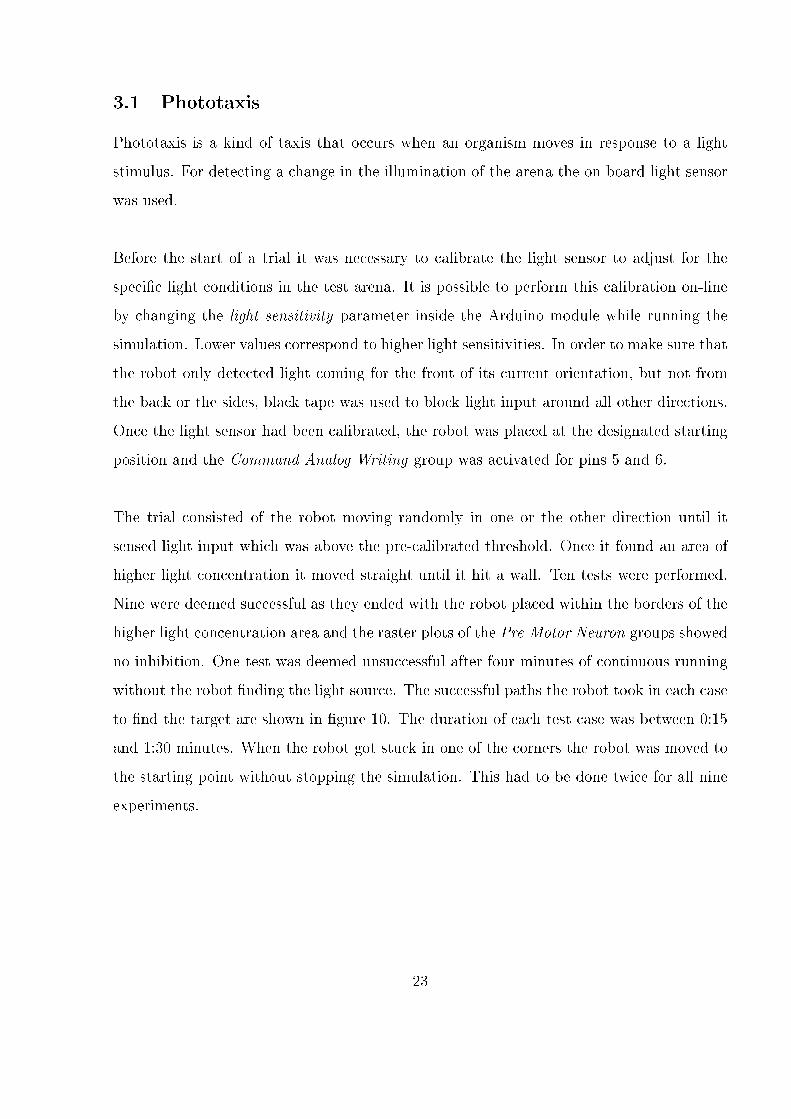
3.1 Phototaxis

Phototaxis is a kind of taxis that occurs when an organism moves in response to a light

stimulus. For detecting a change in the illumination of the arena the on-board light sensor

was used.

Before the start of a trial it was necessary to calibrate the light sensor to adjust for the

speci�c light conditions in the test arena. It is possible to perform this calibration on-line

by changing the light sensitivity parameter inside the Arduino module while running the

simulation. Lower values correspond to higher light sensitivities. In order to make sure that

the robot only detected light coming for the front of its current orientation, but not from

the back or the sides, black tape was used to block light input around all other directions.

Once the light sensor had been calibrated, the robot was placed at the designated starting

position and the Command Analog Writing group was activated for pins 5 and 6.

The trial consisted of the robot moving randomly in one or the other direction until it

sensed light input which was above the pre-calibrated threshold. Once it found an area of

higher light concentration it moved straight until it hit a wall. Ten tests were performed.

Nine were deemed successful as they ended with the robot placed within the borders of the

higher light concentration area and the raster plots of the Pre-Motor Neuron groups showed

no inhibition. One test was deemed unsuccessful after four minutes of continuous running

without the robot �nding the light source. The successful paths the robot took in each case

to �nd the target are shown in �gure 10. The duration of each test case was between 0:15

and 1:30 minutes. When the robot got stuck in one of the corners the robot was moved to

the starting point without stopping the simulation. This had to be done twice for all nine

experiments.

23

0 20 40 60 80 100x position (cm)

0

20

40

60

80

100

y po

sitio

n (c

m)

Figure 10: Path of the robot in the phototaxis test case. The black square indicates the starting position

of the vehicle, and the yellow square shows the part of the arena where the illumination was above threshold.

3.2 Chromatotaxis

Chromatotaxis is the adjustment of movement in response to a color of a speci�c hue. For

the chromatotaxis the HaViMo camera was integrated into the network. The preprocessing

of the camera data was done on the HaViMo chip (see further details in chapter 2.3). The

results were written to pin 13 of the DfRobotShop Rover, so if color was detected, the pin

read HIGH, otherwise LOW. This information was fed into the motor function network

(see �gure 8), using the group Digital Reading in the Arduino module. This served as

sensory input to the motor function network, which sent the output to the Analog Writing

group, pins 5 and 6. Here it was necessary to make some changes to the Arduino module

so it wouldn't interfere with the communication between the camera and the board. Pins

2 and 3 were occupied with serial communication between camera and board so in order to

initialize the other pins for digital reading and analog writing pins 2 and 3 had to be skipped.

Therefore, the group for Digital Reading was of size ten (pins 4-13) and for Analog Writing

only the PWM pins 5,6,9,10,11 were de�ned. This was done to avoid any interference with

the camera. The network was tested on red and blue targets that were placed as shown in

24

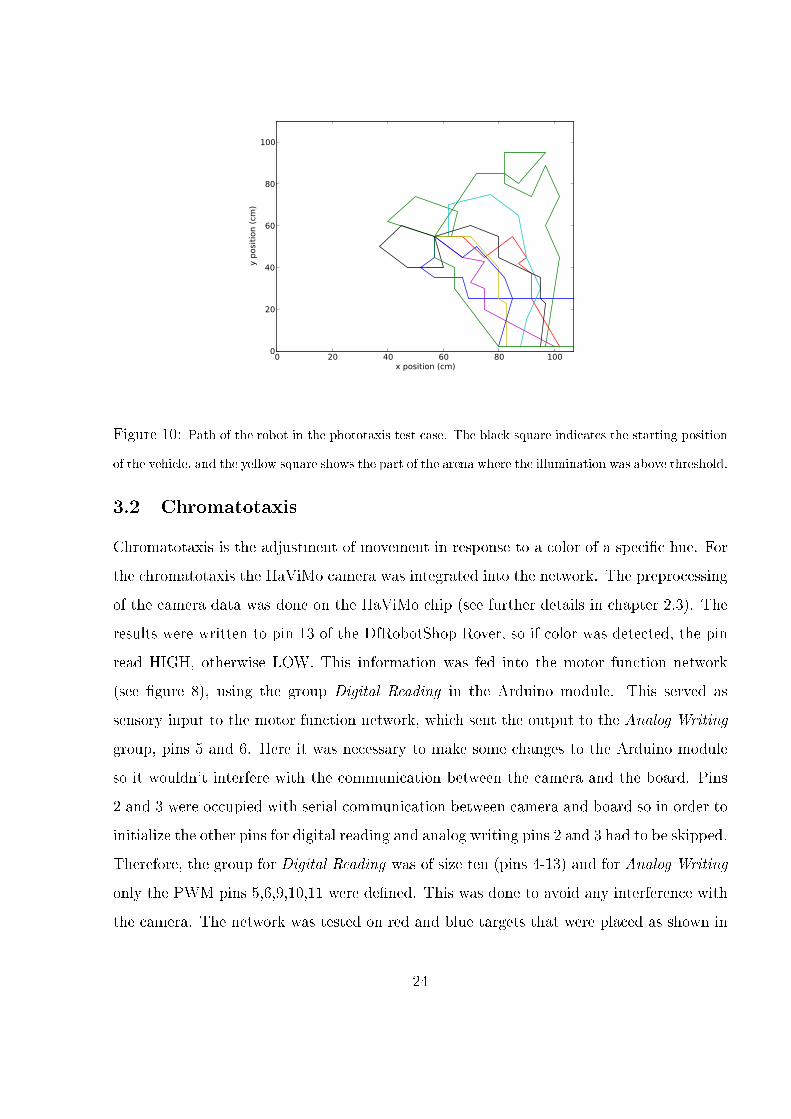
�gure 7. Only one target was presented in each trial.

0 20 40 60 80 100x position (cm)

0

20

40

60

80

100

y po

sitio

n (c

m)

Figure 11: Path of the robot in the chromatotaxis test case for the blue target. The black square indicates

the stating position of the vehicle. The blue circle shows the placement of the target.

Figure 11 shows the path the robot took to successfully �nd the blue target for eight di�erent

test cases. Each trial lasted between 0:30 and 1:30 minutes. Success was only recognized

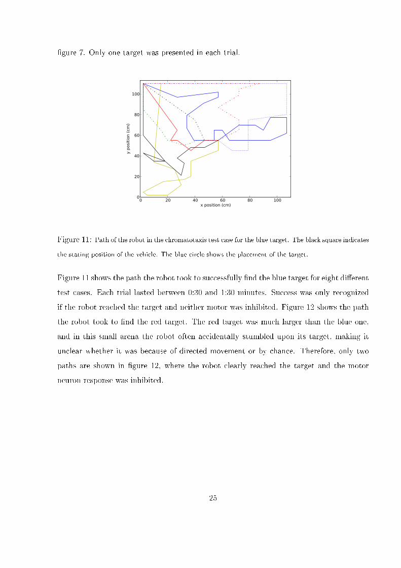
if the robot reached the target and neither motor was inhibited. Figure 12 shows the path

the robot took to �nd the red target. The red target was much larger than the blue one,

and in this small arena the robot often accidentally stumbled upon its target, making it

unclear whether it was because of directed movement or by chance. Therefore, only two

paths are shown in �gure 12, where the robot clearly reached the target and the motor

neuron response was inhibited.

25

0 20 40 60 80 100x position (cm)

0

20

40

60

80

100

y po

sitio

n (c

m)

Figure 12: Path of the robot in the chromatotaxis test case for the red target. The black square indicates

the starting position of the vehicle and the red line the placement of the red target.

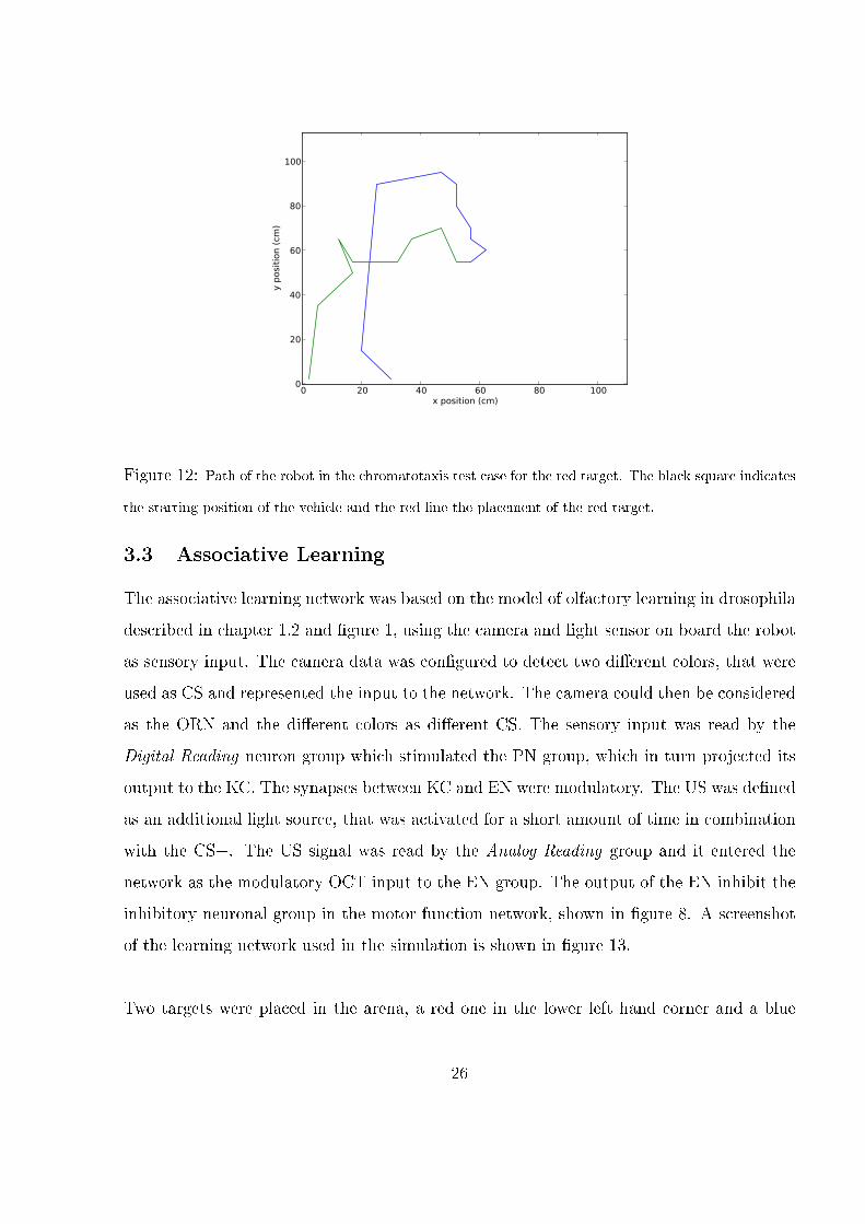
3.3 Associative Learning

The associative learning network was based on the model of olfactory learning in drosophila

described in chapter 1.2 and �gure 1, using the camera and light sensor on board the robot

as sensory input. The camera data was con�gured to detect two di�erent colors, that were

used as CS and represented the input to the network. The camera could then be considered

as the ORN and the di�erent colors as di�erent CS. The sensory input was read by the

Digital Reading neuron group which stimulated the PN group, which in turn projected its

output to the KC. The synapses between KC and EN were modulatory. The US was de�ned

as an additional light source, that was activated for a short amount of time in combination

with the CS+. The US signal was read by the Analog Reading group and it entered the

network as the modulatory OCT input to the EN group. The output of the EN inhibit the

inhibitory neuronal group in the motor function network, shown in �gure 8. A screenshot

of the learning network used in the simulation is shown in �gure 13.

Two targets were placed in the arena, a red one in the lower left hand corner and a blue

26

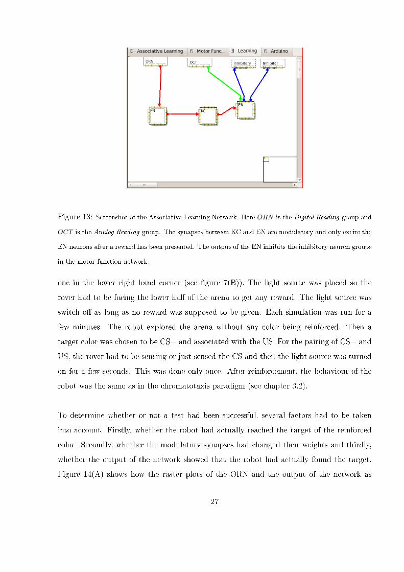
Figure 13: Screenshot of the Associative Learning Network. Here ORN is the Digital Reading group and

OCT is the Analog Reading group. The synapses between KC and EN are modulatory and only excite the

EN neurons after a reward has been presented. The output of the EN inhibits the inhibitory neuron groups

in the motor function network.

one in the lower right hand corner (see �gure 7(B)). The light source was placed so the

rover had to be facing the lower half of the arena to get any reward. The light source was

switch o� as long as no reward was supposed to be given. Each simulation was run for a

few minutes. The robot explored the arena without any color being reinforced. Then a

target color was chosen to be CS+ and associated with the US. For the pairing of CS+ and

US, the rover had to be sensing or just sensed the CS and then the light source was turned

on for a few seconds. This was done only once. After reinforcement, the behaviour of the

robot was the same as in the chromatotaxis paradigm (see chapter 3.2).

To determine whether or not a test had been successful, several factors had to be taken

into account. Firstly, whether the robot had actually reached the target of the reinforced

color. Secondly, whether the modulatory synapses had changed their weights and thirdly,

whether the output of the network showed that the robot had actually found the target.

Figure 14(A) shows how the raster plots of the ORN and the output of the network as

27

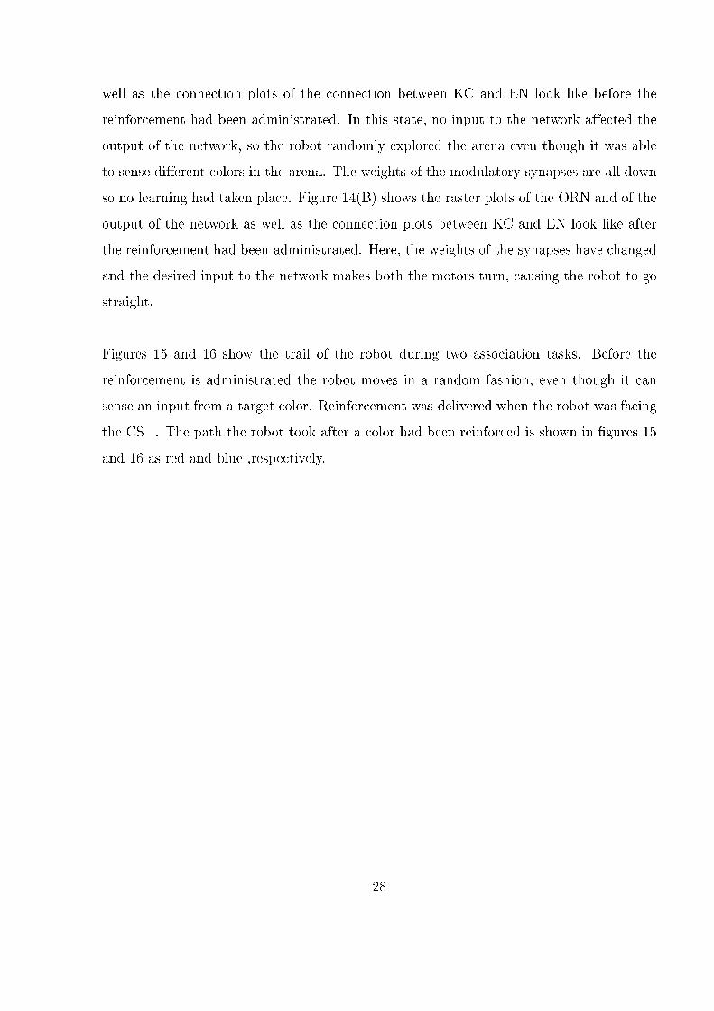
well as the connection plots of the connection between KC and EN look like before the

reinforcement had been administrated. In this state, no input to the network a�ected the

output of the network, so the robot randomly explored the arena even though it was able

to sense di�erent colors in the arena. The weights of the modulatory synapses are all down

so no learning had taken place. Figure 14(B) shows the raster plots of the ORN and of the

output of the network as well as the connection plots between KC and EN look like after

the reinforcement had been administrated. Here, the weights of the synapses have changed

and the desired input to the network makes both the motors turn, causing the robot to go

straight.

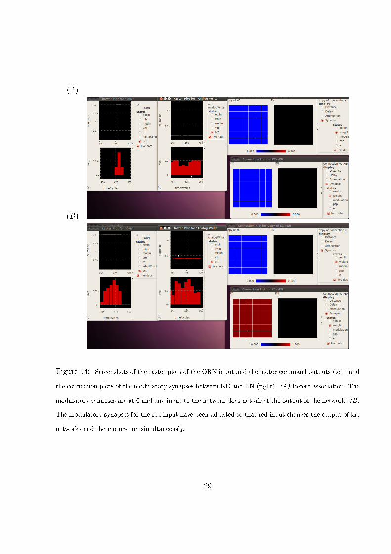
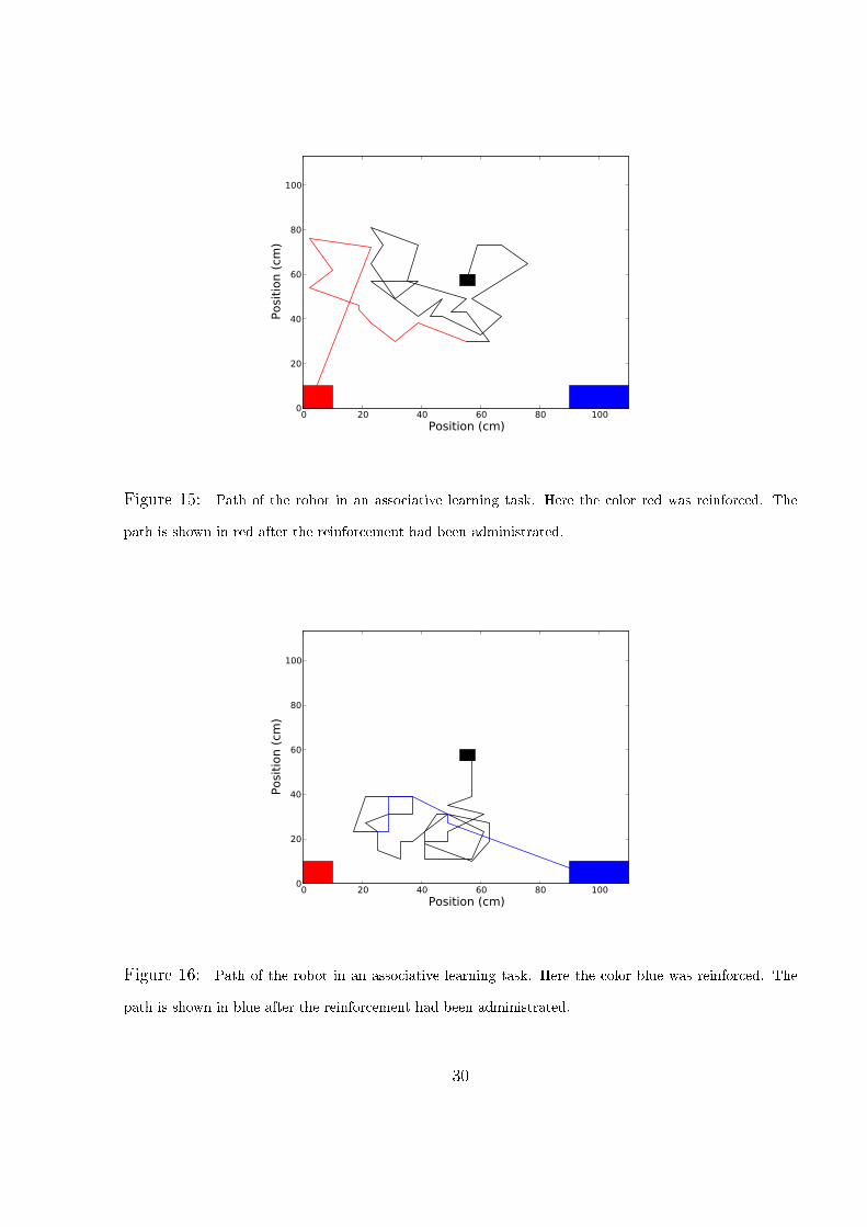
Figures 15 and 16 show the trail of the robot during two association tasks. Before the

reinforcement is administrated the robot moves in a random fashion, even though it can

sense an input from a target color. Reinforcement was delivered when the robot was facing

the CS+. The path the robot took after a color had been reinforced is shown in �gures 15

and 16 as red and blue ,respectively.

28

(A)

(B)

Figure 14: Screenshots of the raster plots of the ORN input and the motor command outputs (left )and

the connection plots of the modulatory synapses between KC and EN (right). (A) Before association. The

modulatory synapses are at 0 and any input to the network does not a�ect the output of the network. (B)

The modulatory synapses for the red input have been adjusted so that red input changes the output of the

networks and the motors run simultaneously.

29

0 20 40 60 80 100Position (cm)

0

20

40

60

80

100

Posi

tion

(cm

)

Figure 15: Path of the robot in an associative learning task. Here the color red was reinforced. The

path is shown in red after the reinforcement had been administrated.

0 20 40 60 80 100Position (cm)

0

20

40

60

80

100

Posi

tion

(cm

)

Figure 16: Path of the robot in an associative learning task. Here the color blue was reinforced. The

path is shown in blue after the reinforcement had been administrated.

30

4 Conclusions and Future Work

In the work at hand, a new and inexpensive platform that uses a SNN simulator to control

a robot was presented. It is easy to set up and use. The on-board light sensor and the

added HaViMo camera provide real-time sensory information that can be fed into a SNN

simulator. The simulated network is then used to as a control architecture for the robot.

The three test cases presented, phototaxis, chromatotaxis and associative learning, were

all executed successfully in a small arena, with the robot readily approaching its targets in

most trials.

The motor function network did not follow any exploration algorithm, but created random

activity in either of the motors, when no sensory input was presented, but simultaneous

activity in the presence of sensory input. When the robot lost sight of its target, it would

again move randomly in some direction. This sometimes lead to the robot moving away

from the target after it had sensed it, even if it had lost sight of it only for a short amount

of time. This made it sometimes hard to realize if the robot had actually found the target

or not, without reading raster plots of the output of the network.

In the phototaxis test case illuminated above threshold in only one corner of the arena,

while the rest of the arena was lit subthreshold. The current network versions does not

allow for a representation of gradual changes of the external illumination. Therefore, the

robot had to stumble upon the edges of the corner by accident to sense the higher light

concentration. To make it more likely for the robot to accidentally �nd the edges of the

corner, the robot was placed with the edge on the right side of it so there was a 50% chance

of the robot to turn initially the right way. In one case the robot never found the edge

of the higher illuminated corner by accident and after four minutes of trial and error the

simulation was stopped.

31

For the chromatotaxis test case the red target turned out to be too big, which resulted

in the robot often reaching it without purposely approaching it. Finding the blue target

proved to be successful in every case that was tested. A correct calibration of the camera

was the most important aspect in the chromatotaxis test case. A small amount of pixels in

the captured image were su�cient to detect a color in the image. This could lead to some

small patches of pixels not belonging to a target being detected erroneously and undesirably

in�uencing the behaviour of the robot. This could be avoided by adding a error detection

to the Arduino �rmware, but this has not yet been implemented.

The associative learning test case showed how powerful indeed the platform is. By combin-

ing sensory input from the light sensor and the camera and adding a learning rule based

on the model of the olfactory learning in insects, we could make the robot associate a color

(CS) with a reward (US). The synchronization of a stimulus and a reward was the biggest

challenge. When it was correctly executed, the robot showed the expected behaviour. How-

ever, the real-time processing of the sensory data is limited to the processing power of the

workstation running the simulation. Although the delay between sensory input and the

output of the network reaching the motors of the robot was only about a second, it could

cause the robot to move slightly away from its target.

This platform opens up many opportunities to test di�erent SNN models of learning and

memory, using robots. Adding prede�ned motivational states and testing out biologically

inspired exploration algorithms would be an interesting next step to apply the abilities

of the platform. This platform could also be used to create a control SNN for the robot

which starts learning with minimal knowledge about the environment. Another option is

to create and test networks for operand conditioning, where certain actions are reinforced.

The real time processing of the sensory data limits the number of neurons and connections

of a network, reducing its potential computational power. This makes it hard to mimic

the information processing of biological system, but with faster computers, more realistic

simulations can be performed.

32

References

[1] Socat. http://www.dest-unreach.org/socat/doc/socat.html, Dec 2011.

[2] Arduino duemilanove. http://arduino.cc/en/Main/, June 2012.

[3] Ulysses Bernardet and Paul Verschure. iqr: A tool for the construction of multi-level

simulations of brain and behaviour. Neuroinformatics, 8:113�134, 2010.

[4] M.E. Bitterman, R. Menzel, A Fietz, and S. Schäfer. Classical conditioning of proboscis

extension in honeybees (apis mellifera). Journal of comparative psychology, 97(2):107�

119, June 1983.

[5] Stijn Cassenaer and Gilles Laurent. Conditional modulation of spike-timing-dependent

plasticity for olfactory learning. Nature, Jan 2012.

[6] Brian R. Cox and Je�rey L. Krichmar. Neuromodulation as a robot controller: A brain

inspired strategy for controlling autonomous robots. IEEE Robotics and Automation

Magazine, 16(3):72�80, 2009.

[7] Peter Dayan and L.F. Abbott. Theoretical Neuroscience: Computational and Math-

ematical Modeling of Neural Systems. The MIT Press, Cambridge, Massachusetts,

2001.

[8] Adam Dunkels, Oliver Schmidt, Thiemo Voigt, and Muneeb Ali. Protothreads: Simpli-

fying event-driven programming of memory-constrained embedded systems. In Proceed-

ings of the Fourth ACM Conference on Embedded Networked Sensor Systems (SenSys

2006), Boulder, Colorado, USA, November 2006.

[9] Hani Hagras, Anthony Pounds-Cornish, Martin Colley, Victor Callaghan, and Gra-

ham Clarke. Evolving spiking neural network controllers for autonomous robots. In

Proceedings of the 2004 IEEE International Conference on Robotics and Automation,

pages 4620�4626, 2004.

[10] Je�ery L. Krichmar. Neurorobotics. Scholarpedia, 3(3):1365, 2008.

33

[11] Wolfgang Maass. Pulsed Neural Networks, chapter Computing with spiking neurons.

WA:Bratford Books, 1999.

[12] Jan Meyer, Joachim Haenicke, Tim Landgraf, Michael Schmuker, Raúl Rojas, and

Martin Nawrot. A digital receptor neuron connecting remote sensor hardware to spik-

ing neural networks. Frontiers in Computational Neuroscience, (00164).

[13] Ben Mitchinson, Martin J. Pearson, Anthony G. Pipe, and Tony J. Prescott. Neu-

romorphic and Brain-Based Robots, chapter Biometric robots as scienti�c models: a

view from the whisker tip. Cambridge Univesity Press, 2011.

[14] Hamid Moballegh. HaViMo2 - Image Processing Module, March 2010.

[15] RobotShop Inc., www.RobotShop.com. DfRobotShop Rover User Guide v2.1, Jan 2012.

[16] J. C. Sandoz. Behavioral and neurophysiological study of olfactory perception and

learning in honeybees. Frontiers in systems neuroscience, 5, January 2011.

[17] S. Soltic and N. Kasabov. System and Circuit design for Biologically-Inspired Intel-

ligent Learning, chapter A Biologically Inspired Evolving Spiking Neural Model with

Rank-Order Population Coding and a Taste Recognition System Case Study. Medical

Information Science Reference, 2011.

[18] Jilles Vreeken. Spiking neural networks, an introduction. Technical report, Institute

for Information and Computing Sciences� Utrecht University, 2002.

[19] Barbara Webb. Animals versus animats: Or why not model the real iguana? Adaptive

Behavior - Animals, Animats, Software Agents, Robots, Adaptive Systems, 17(4):269�

286, August 2009.

[20] Jan Wessnitzer, Joanna M. Young, J. Douglas Armstrong, and Barbara Webb. A model

of non-elemental olfactory learning in drosophila. J. Comput. Neurosci., 32(2):197�212,

April 2012.

[21] WIZnet Co Ltd. WizFi210/220 User Manual, v1.0 edition, March 2011.

34

A Wireless Communication

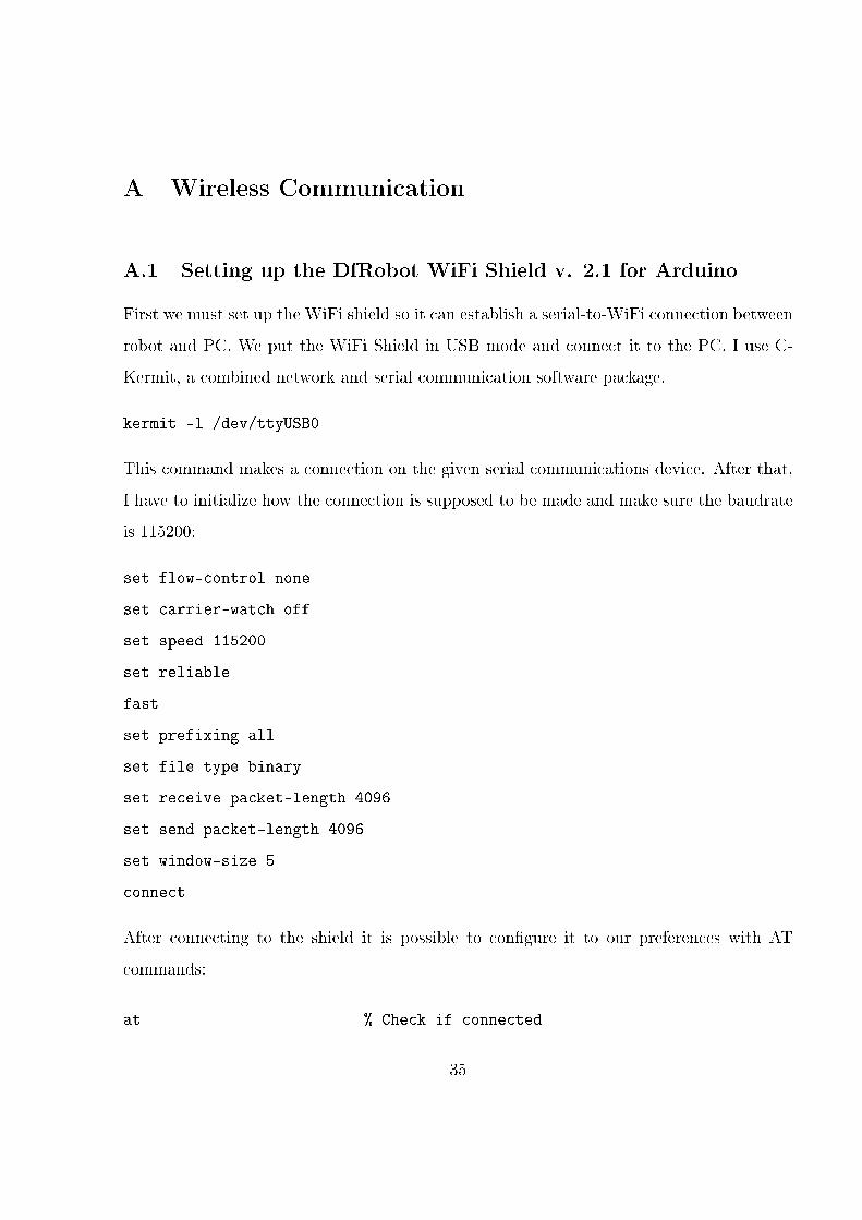
A.1 Setting up the DfRobot WiFi Shield v. 2.1 for Arduino

First we must set up the WiFi shield so it can establish a serial-to-WiFi connection between

robot and PC. We put the WiFi Shield in USB mode and connect it to the PC. I use C-

Kermit, a combined network and serial communication software package.

kermit -l /dev/ttyUSB0

This command makes a connection on the given serial communications device. After that,

I have to initialize how the connection is supposed to be made and make sure the baudrate

is 115200:

set flow-control none

set carrier-watch off

set speed 115200

set reliable

fast

set prefixing all

set file type binary

set receive packet-length 4096

set send packet-length 4096

set window-size 5

connect

After connecting to the shield it is possible to con�gure it to our preferences with AT

commands:

at % Check if connected

35

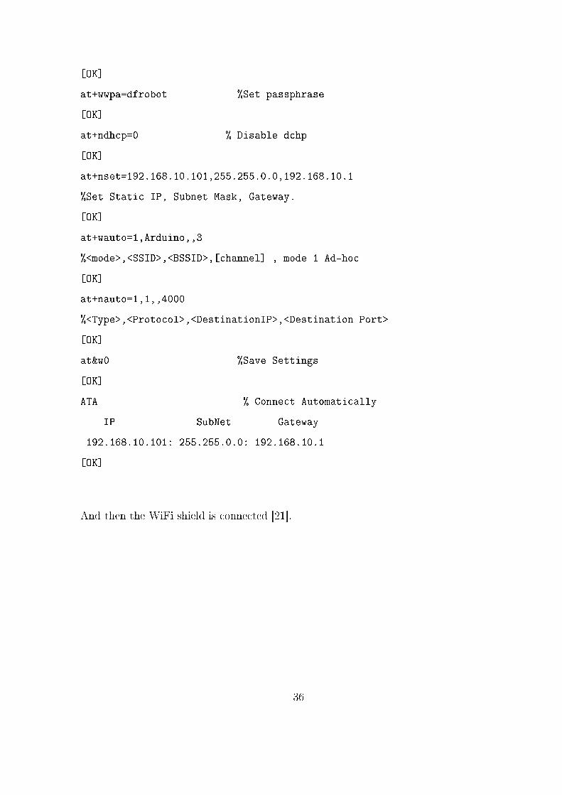
[OK]

at+wwpa=dfrobot %Set passphrase

[OK]

at+ndhcp=0 % Disable dchp

[OK]

at+nset=192.168.10.101,255.255.0.0,192.168.10.1

%Set Static IP, Subnet Mask, Gateway.

[OK]

at+wauto=1,Arduino,,3

%<mode>,<SSID>,<BSSID>,[channel] , mode 1 Ad-hoc

[OK]

at+nauto=1,1,,4000

%<Type>,<Protocol>,<DestinationIP>,<Destination Port>

[OK]

at&w0 %Save Settings

[OK]

ATA % Connect Automatically

IP SubNet Gateway

192.168.10.101: 255.255.0.0: 192.168.10.1

[OK]

And then the WiFi shield is connected [21].

36

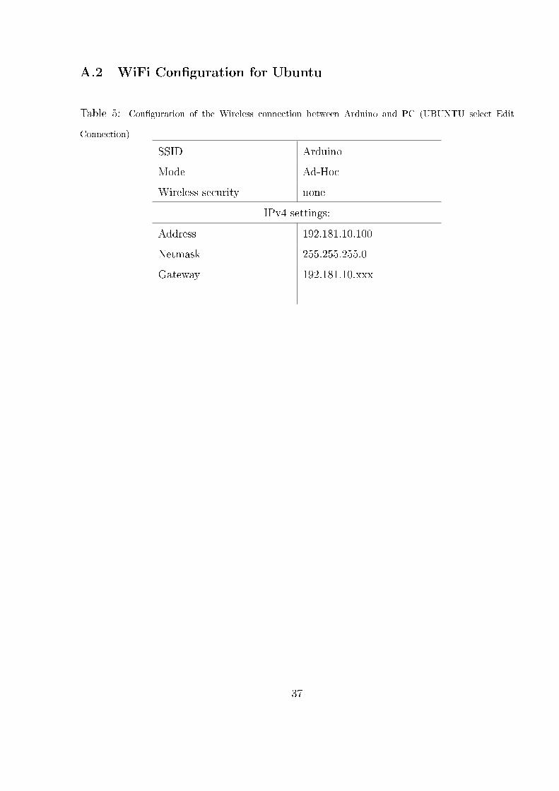
A.2 WiFi Con�guration for Ubuntu

Table 5: Con�guration of the Wireless connection between Arduino and PC (UBUNTU select Edit

Connection)

SSID Arduino

Mode Ad-Hoc

Wireless security none

IPv4 settings:

Address 192.181.10.100

Netmask 255.255.255.0

Gateway 192.181.10.xxx

37

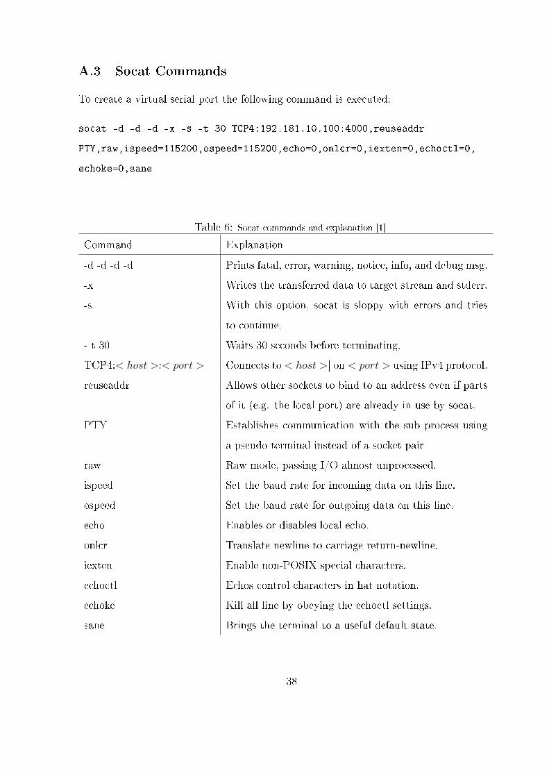
A.3 Socat Commands

To create a virtual serial port the following command is executed:

socat -d -d -d -x -s -t 30 TCP4:192.181.10.100:4000,reuseaddr

PTY,raw,ispeed=115200,ospeed=115200,echo=0,onlcr=0,iexten=0,echoctl=0,

echoke=0,sane

Table 6: Socat commands and explanation [1]

Command Explanation

-d -d -d -d Prints fatal, error, warning, notice, info, and debug msg.

-x Writes the transferred data to target stream and stderr.

-s With this option, socat is sloppy with errors and tries

to continue.

- t 30 Waits 30 seconds before terminating.

TCP4:< host >:< port > Connects to < host >] on < port > using IPv4 protocol.

reuseaddr Allows other sockets to bind to an address even if parts

of it (e.g. the local port) are already in use by socat.

PTY Establishes communication with the sub process using

a pseudo terminal instead of a socket pair

raw Raw mode, passing I/O almost unprocessed.

ispeed Set the baud rate for incoming data on this line.

ospeed Set the baud rate for outgoing data on this line.

echo Enables or disables local echo.

onlcr Translate newline to carriage return-newline.

iexten Enable non-POSIX special characters.

echoctl Echos control characters in hat notation.

echoke Kill all line by obeying the echoctl settings.

sane Brings the terminal to a useful default state.

38

B Code

B.1 Arduino Firmware

1 // S e r i a l I n t e r f a c e wi th th read ing

2 // Author : Lovisa Irpa He l g ado t t i r

3 #include <So f twa r eS e r i a l . h>

4 #include <havimo . h>

5 #include <pt . h>

6

7 // Havimo

8 #define rxPin 2

9 #define txPin 3

10 HaViMo havimo ( rxPin , txPin , 1 1 5200 ) ;

11

12 // Def in ing Threads

13 stat ic struct pt pt1 , pt2 ;

14

15 // I n s t r u c t i o n s

16 int const PIN_MODE = 0 ;

17 int const DIGITAL_READ = 1 ;

18 int const DIGITAL_WRITE = 2 ;

19 int const ANALOG_REFERENCE = 3 ;

20 int const ANALOG_READ = 4 ;

21 int const ANALOG_WRITE = 5 ;

22

23 // Constants

24 int const H = 1 ;

25 int const L = 0 ;

26 byte com , pin , s ta r t , va lue ;

27

28 stat ic int s e r i a l I n t e r f a c eTh r e ad ( struct pt ∗pt ){ // S e r i a l i n t e r f a c e thread

39

29 PT_BEGIN( pt ) ;

30 i f ( S e r i a l . a v a i l a b l e ()>0){

31 s t a r t=getCommand ( ) ;

32 while ( s t a r t !=0){ s t a r t=getCommand ( ) ; }

33 S e r i a l . p r i n t ( s t a r t ) ;

34 com=getCommand ( ) ;

35 S e r i a l . p r i n t (com ) ;



38 pin=getCommand ( ) ;

39 S e r i a l . p r i n t ( pin ) ;

40

41 i f (com==PIN_MODE | | com==DIGITAL_WRITE) {



44 value=getCommand ( ) ;

45 S e r i a l . p r i n t ( va lue ) ;

46 a l lFunc (com , pin , va lue ) ; }

47

48 i f (com==DIGITAL_READ | | com==ANALOG_READ){


50 value=al lFunc (com , pin , 0 ) ; }

51 S e r i a l . p r i n t ( va lue ) ; }

52

53 i f (com==ANALOG_WRITE){



56 value=getCommand ( ) ;

57 i f ( value <100){ S e r i a l . p r i n t ( s t a r t ) ; }

58 i f ( value <10){ S e r i a l . p r i n t ( s t a r t ) ; }

59 S e r i a l . p r i n t ( va lue ) ;

60 a l lFunc (com , pin , va lue ) ; }

61 }

62 PT_END( pt ) ;

63 }

64

40

65 stat ic int havimoThread ( struct pt ∗pt ){

66 PT_BEGIN( pt ) ;

67

68 int c [ 1 6 ] , d [ 1 6 ] ; // crea t e con ta iner s

69

70 pinMode (12 ,OUTPUT) ; // Set p ins as output

71 pinMode (13 ,OUTPUT) ;

72

73 havimo . captureRegion ( ) ; //Capture and read image

74 havimo . readRegion (1 , c ) ;

75 havimo . readRegion (2 , d ) ;

76

77 i f ( c [1]==2 | | d [1]==2){ a l lFunc (DIGITAL_WRITE, 1 2 , 1 ) ; } // co l o r 2

78 else { a l lFunc (DIGITAL_WRITE, 1 2 , 0 ) ; }

79

80 i f ( c [1]==1 | | ( c [1]==2 && d[1]==1)){ a l lFunc (DIGITAL_WRITE, 1 3 , 1 ) ; } // co l o r 1

81 else { a l lFunc (DIGITAL_WRITE, 1 3 , 0 ) ; }

82 PT_END( pt ) ;

83 }

84

85 int getCommand (){ // ge t s e r i a l commands

86 int m=Se r i a l . read ( ) ;

87 return m;

88 }

89

90 int a l lFunc ( int com , int pin , int value ){ // Switch arduino f unc t i on s

91 int va l ;

92 switch (com){

93 case PIN_MODE:

94 pinMode ( pin , va lue ) ;

95 case DIGITAL_READ:

96 return d ig i t a lRead ( pin ) ;

97 break ;

98 case DIGITAL_WRITE:

99 d i g i t a lWr i t e ( pin , va lue ) ;

100 break ;

41

101 case ANALOG_READ:

102 va l= analogRead ( pin ) ;

103 i f ( va l <100){ S e r i a l . p r i n t ( 0 ) ; }

104 i f ( val <10){ S e r i a l . p r i n t ( 0 ) ; }

105 return va l ;

106 break ;

107 case ANALOG_WRITE:

108 analogWrite ( pin , va lue ) ;

109 break ;

110 default :

111 break ;

112 }

113 }

114 void setup ( ){

115 S e r i a l . begin (115200 ) ;

116 S e r i a l . f l u s h ( ) ;

117 PT_INIT(&pt1 ) ;

118 PT_INIT(&pt2 ) ;

119 }

120 void loop ( ){

121 havimoThread(&pt2 ) ;

122 s e r i a l I n t e r f a c eTh r e ad (&pt1 ) ;

123 }

42

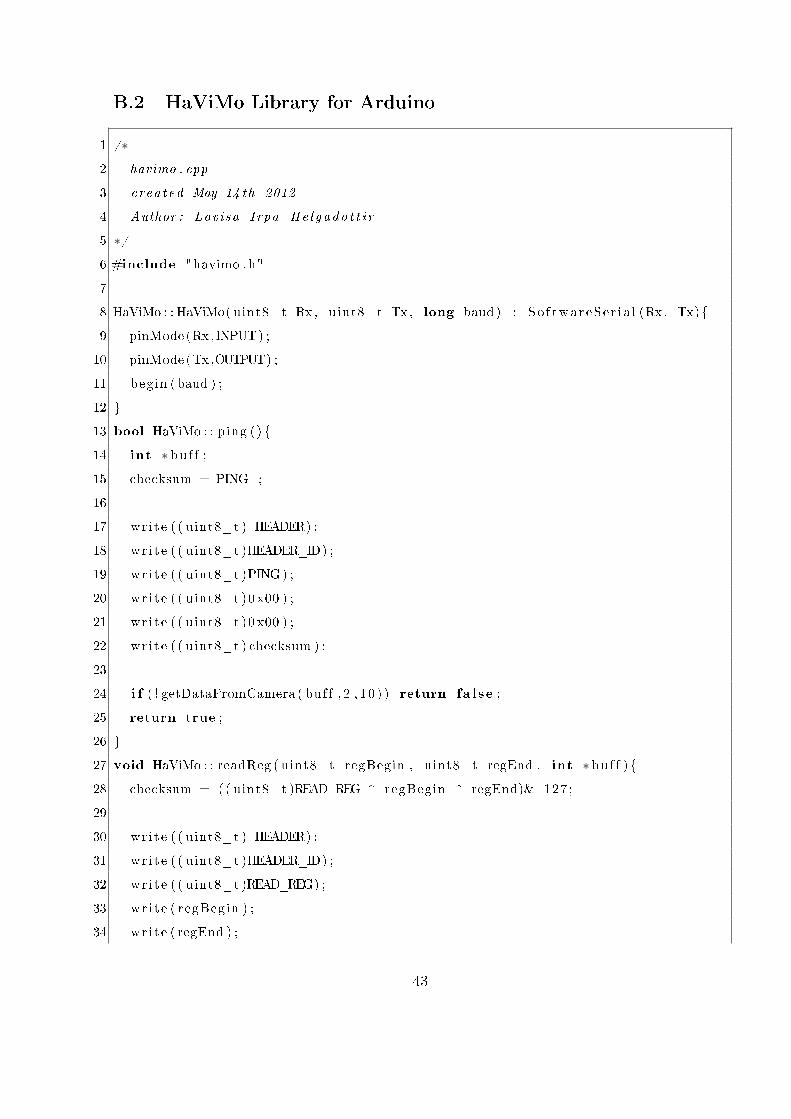
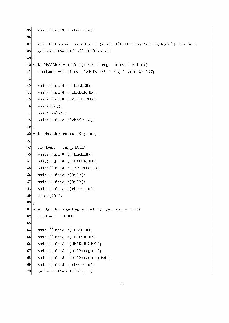
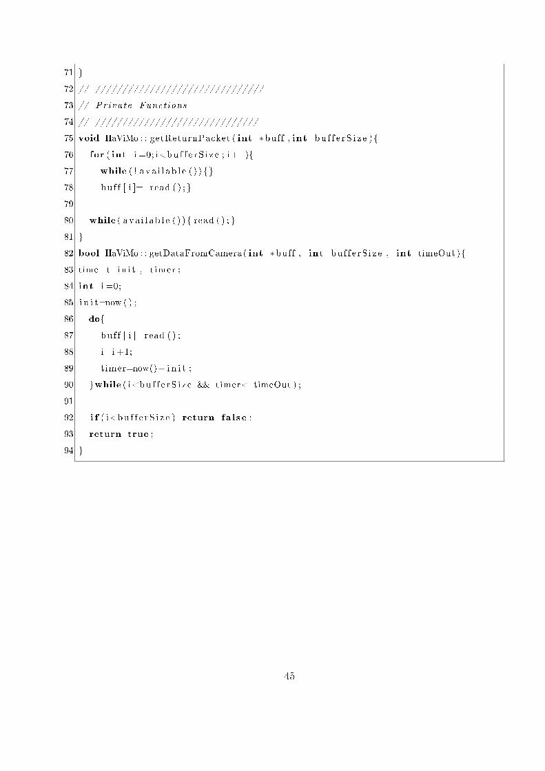
B.2 HaViMo Library for Arduino

1 /∗

2 havimo . cpp

3 crea t ed May 14 th 2012

4 Author : Lovisa Irpa He l g ado t t i r

5 ∗/

6 #include "havimo . h"

7

8 HaViMo : : HaViMo( uint8_t Rx , uint8_t Tx , long baud ) : So f twa r eS e r i a l (Rx , Tx){

9 pinMode (Rx ,INPUT) ;

10 pinMode (Tx ,OUTPUT) ;

11 begin ( baud ) ;

12 }

13 bool HaViMo : : ping ( ){

14 int ∗ bu f f ;

15 checksum = PING ;

16

17 wr i t e ( ( uint8_t ) HEADER) ;

18 wr i t e ( ( uint8_t )HEADER_ID) ;

19 wr i t e ( ( uint8_t )PING) ;

20 wr i t e ( ( uint8_t )0 x00 ) ;

21 wr i t e ( ( uint8_t )0 x00 ) ;

22 wr i t e ( ( uint8_t ) checksum ) ;

23

24 i f ( ! getDataFromCamera ( buf f , 2 , 1 0 ) ) return fa l se ;

25 return true ;

26 }

27 void HaViMo : : readReg ( uint8_t regBegin , uint8_t regEnd , int ∗ bu f f ){

28 checksum = (( uint8_t )READ_REG ^ regBegin ^ regEnd)& 127 ;

29



32 wr i t e ( ( uint8_t )READ_REG) ;

33 wr i t e ( regBegin ) ;

34 wr i t e ( regEnd ) ;

43


36

37 int Bu f f e r s i z e =(regBegin !=( uint8_t )0 x00 )? ( regEnd−regBegin )+1: regEnd ;

38 getReturnPacket ( buf f , Bu f f e r s i z e ) ;

39 }

40 void HaViMo : : writeReg ( uint8_t reg , uint8_t value ){

41 checksum = (( uint8_t )WRITE_REG ^ reg ^ value)& 127 ;

42



45 wr i t e ( ( uint8_t )WRITE_REG) ;

46 wr i t e ( reg ) ;

47 wr i t e ( va lue ) ;


49 }

50 void HaViMo : : captureRegion ( ){

51

52 checksum = CAP_REGION;



55 wr i t e ( ( uint8_t )CAP_REGION) ;

56 wr i t e ( ( uint8_t )0 x00 ) ;

57 wr i t e ( ( uint8_t )0 x00 ) ;


59 de lay ( 2 0 0 ) ;

60 }

61 void HaViMo : : readRegion ( int reg ion , int ∗ bu f f ){

62 checksum = 0x0D ;

63



66 wr i t e ( ( uint8_t )READ_REGION) ;

67 wr i t e ( ( uint8_t )0 x10∗ r eg i on ) ;

68 wr i t e ( ( uint8_t )0 x10∗ r eg i on+0x0F ) ;


70 getReturnPacket ( buf f , 1 6 ) ;

44

71 }

72 // ///////////////////////////////

73 // Pr iva te Functions

74 // //////////////////////////////

75 void HaViMo : : getReturnPacket ( int ∗buf f , int bu f f e r S i z e ){

76 for ( int i =0; i<bu f f e r S i z e ; i++){

77 while ( ! a v a i l a b l e ( ) ) {}

78 bu f f [ i ]= read ( ) ; }

79

80 while ( a v a i l a b l e ( ) ) { read ( ) ; }

81 }

82 bool HaViMo : : getDataFromCamera ( int ∗buf f , int bu f f e r S i z e , int timeOut ){

83 time_t i n i t , t imer ;

84 int i =0;

85 i n i t=now ( ) ;

86 do{

87 bu f f [ i ]= read ( ) ;

88 i=i +1;

89 t imer=now()− i n i t ;

90 }while ( i<bu f f e r S i z e && timer< timeOut ) ;

91

92 i f ( i<bu f f e r S i z e ) return fa l se ;

93 return true ;

94 }

45

controlling an autonomous robot using spiking neural · pdf filecontrolling an autonomous...

Documents