controlling a quadrotor with a robotic arm using … this thesis designs a method to control a...
TRANSCRIPT
Universitat Politecnica de Catalunya
Master Thesis
Controlling a Quadrotor with a RoboticArm using Nonlinear Model Predictive
Control
Author:
Sebastian Chavez-Ferrer Marcos
Supervisors:
Dr. Carlos Ocampo Martınez
Institut de Robotica i Informatica Industrial (CSIC-UPC)
February 2015

Acknowledgements
I would like to express my gratitude to the Master coordinator, Cecilio Angulo, who
helped me to solve all my administrative problems and also who showed me the benefits
of the master.
Also, I would like to thank my supervisor Carlos Ocampo, who guided me through the
good and bad moments of the thesis. Without his help it would have been impossible
to finish it.
On the other hand, I would like to express my appreciation to all the people from the
Institut de Robotica i Informatica Industrial (IRI) where I was very well welcomed.
I would like to thank all the people who suffered and enjoyed this Master with me, my
class colleagues from the MAiR and my friends from ETSEIB.
Additionally, I would like to thank Victor, Neus and Paula to help me finish this project.
Finally I would like to express my biggest acknowledgements to my parents, who sup-
ported me and encouraged me until the end of my studies.
iii

Abstract
This thesis designs a method to control a quadrotor equipped with a robotic arm. The
arm has been developed in Institut de Robotica i Informatica Industrial (CSIC-UPC),
namely here IRI. During the project, an algorithm has been made as a first approxima-
tion to control a quadrotor that is working with the robotic arm. In order to compensate
the perturbations of the arm’s dynamic, a NMPC algorithm has been chosen while oth-
ers have been discarded as it is discussed in the state of the art (PID, Linear Model
Predictive Control or LQR).
PID and model predictive control have been discarded because is not possible to handle
the nonlinearities of the system studied and reach the desired control objectives. Also
there are no possibilites to restrict the system using physical constraints. Finally, three
scenarios have been simulated and tested to verify the performances and robustness
of the designed method. A takeoff maneuver, where the quadrotor reaches a specific
altitude. A hover mode where the system should compensate the dynamics of the arm
while it is static or it is in movement. Finally, the quadorotor has to move to a specific
point in the space while the arm it is static or in movement. The goal of the controller
is to reject the perturbation due the movement of the arm and stabilize the system.
This thesis presents the results obtained after simulating the designed controller with
the scenarios considered.

Contents
Acknowledgements iii
Abstract v
List of Figures ix
List of Tables xi
Nomenclature xiii
1 Introduction 1
1.1 Motivation . . . . . . . . . . . . . . . . . . . . . . . . . . . . . . . . . . . 1
1.2 Objectives . . . . . . . . . . . . . . . . . . . . . . . . . . . . . . . . . . . . 2
1.3 Scope of Research . . . . . . . . . . . . . . . . . . . . . . . . . . . . . . . 2
1.4 Outline of the Thesis . . . . . . . . . . . . . . . . . . . . . . . . . . . . . . 3
2 Background 5
2.1 Unmanned Aerial Vehicles . . . . . . . . . . . . . . . . . . . . . . . . . . . 6
2.2 Robotic Arms . . . . . . . . . . . . . . . . . . . . . . . . . . . . . . . . . . 7
2.3 Control Algorithm . . . . . . . . . . . . . . . . . . . . . . . . . . . . . . . 8
2.4 State of the Art . . . . . . . . . . . . . . . . . . . . . . . . . . . . . . . . . 12
3 Case Study Description and Control Problem 15
3.1 Quadrotor Description . . . . . . . . . . . . . . . . . . . . . . . . . . . . . 15
3.1.1 Dynamic Equations of a X-Type Quadrotor . . . . . . . . . . . . . 15
3.1.2 Dynamic Equations to Simulate the Real Plant . . . . . . . . . . . 22
3.1.3 Physical and Geometrical Parameters of the Quadrotor Model . . 23
3.2 Robotic Arm Description . . . . . . . . . . . . . . . . . . . . . . . . . . . 24
3.2.1 Dynamic Equations of a Robotic Arm . . . . . . . . . . . . . . . . 24
3.2.2 Dynamic Equations to Simulate the Real Robotic Arm . . . . . . . 27
3.2.3 Physical and Geometrical Parameters of the Arm Model . . . . . . 28
3.3 NMPC Problem Statement . . . . . . . . . . . . . . . . . . . . . . . . . . 30
3.3.1 Dynamic Model . . . . . . . . . . . . . . . . . . . . . . . . . . . . . 30
3.3.2 Objective Function . . . . . . . . . . . . . . . . . . . . . . . . . . . 33
3.3.3 Constraints . . . . . . . . . . . . . . . . . . . . . . . . . . . . . . . 35
3.3.4 Optimization Problem . . . . . . . . . . . . . . . . . . . . . . . . . 38
4 Simulation Results 41
4.1 Take off . . . . . . . . . . . . . . . . . . . . . . . . . . . . . . . . . . . . . 45
vii
Contents viii
4.2 Quadrotor in a fixed position . . . . . . . . . . . . . . . . . . . . . . . . . 50
4.2.1 Robotic Arm in a Fixed Position . . . . . . . . . . . . . . . . . . . 51
4.2.2 Robotic Arm in Movement . . . . . . . . . . . . . . . . . . . . . . 53
4.3 Quadrotor in Movement . . . . . . . . . . . . . . . . . . . . . . . . . . . . 54
4.3.1 Robotic Arm in a Fixed Position . . . . . . . . . . . . . . . . . . . 55
4.3.2 Robotic Arm in Movement . . . . . . . . . . . . . . . . . . . . . . 57
5 Conclusions and Future Work 61
5.1 Conclusions . . . . . . . . . . . . . . . . . . . . . . . . . . . . . . . . . . . 61
5.2 Future Work . . . . . . . . . . . . . . . . . . . . . . . . . . . . . . . . . . 62
Bibliography 65
List of Figures
2.1 Top-Left: X-Type. Top-Right: V-Type. Bottom: Stingray-Type . . . . . 7
2.2 Robotic arm designed by IRI . . . . . . . . . . . . . . . . . . . . . . . . . 8
2.3 Scheme of MPC algorithm . . . . . . . . . . . . . . . . . . . . . . . . . . . 10
2.4 NMPC scheme . . . . . . . . . . . . . . . . . . . . . . . . . . . . . . . . . 11
2.5 Examples of UAV . . . . . . . . . . . . . . . . . . . . . . . . . . . . . . . . 12
3.1 Blade system reference . . . . . . . . . . . . . . . . . . . . . . . . . . . . . 16
3.2 Forward-Backward movement . . . . . . . . . . . . . . . . . . . . . . . . . 18
3.3 Left-Right movement . . . . . . . . . . . . . . . . . . . . . . . . . . . . . . 19
3.4 Up-Down movement . . . . . . . . . . . . . . . . . . . . . . . . . . . . . . 19
3.5 Rotate around E3a . . . . . . . . . . . . . . . . . . . . . . . . . . . . . . . 19
3.6 Parameters of a blade . . . . . . . . . . . . . . . . . . . . . . . . . . . . . 20
3.7 Denavit hartenberg parameters . . . . . . . . . . . . . . . . . . . . . . . . 25
3.8 Matlab model of the robotic arm designed by IRI. . . . . . . . . . . . . . 29
4.1 Dynamic reaction in the base of the arm remaining in a fixed position . . 43
4.2 Reference and Angle of each joint . . . . . . . . . . . . . . . . . . . . . . . 44
4.3 Dynamic Reaction in the base of the arm due its motion . . . . . . . . . . 45
4.4 Cost function during the Take Off . . . . . . . . . . . . . . . . . . . . . . 47
4.5 Control signal for a Takeoff . . . . . . . . . . . . . . . . . . . . . . . . . . 48
4.6 State variables for the Takeoff . . . . . . . . . . . . . . . . . . . . . . . . . 49
4.7 State variables for a quadrotor in a fixed position and an arm in a fixedposition . . . . . . . . . . . . . . . . . . . . . . . . . . . . . . . . . . . . . 51
4.8 Cost function for a quadrotor in a fixed position and an arm in a fixedposition . . . . . . . . . . . . . . . . . . . . . . . . . . . . . . . . . . . . . 52
4.9 State variables for a quadrotor in a fixed position and an arm in movement 53
4.10 Cost function for a quadrotor in a fixed position and an arm in movement 54
4.11 Cost function for a quadrotor in movement and an arm in a fixed position 55
4.12 State variables for a quadrotor in movement and an arm in a fixed position 57
4.13 Cost function for a quadrotor in movement and an arm in movement . . . 58
4.14 State variables for a quadrotor in movement and an arm in movement . . 59
ix

List of Tables
3.1 DH parameters of the robotic arm . . . . . . . . . . . . . . . . . . . . . . 30
4.1 Initial Conditions for Take Off . . . . . . . . . . . . . . . . . . . . . . . . 47
4.2 Summary of Take Off . . . . . . . . . . . . . . . . . . . . . . . . . . . . . 49
4.3 Initial Conditions for Static Control . . . . . . . . . . . . . . . . . . . . . 50
4.4 Summary of the control for a quadrotor in a fixed position and an arm ina fixed position . . . . . . . . . . . . . . . . . . . . . . . . . . . . . . . . . 52
4.5 Summary of the control for a quadrotor in a fixed position and an arm inmovement . . . . . . . . . . . . . . . . . . . . . . . . . . . . . . . . . . . . 54
4.6 Initial Conditions for quadrotor in movement . . . . . . . . . . . . . . . . 55
4.7 Summary of the control for a quadrotor in movement and an arm in afixed position . . . . . . . . . . . . . . . . . . . . . . . . . . . . . . . . . . 56
4.8 Summary of the control for a quadrotor in movement and an arm inmovement . . . . . . . . . . . . . . . . . . . . . . . . . . . . . . . . . . . . 58
xi

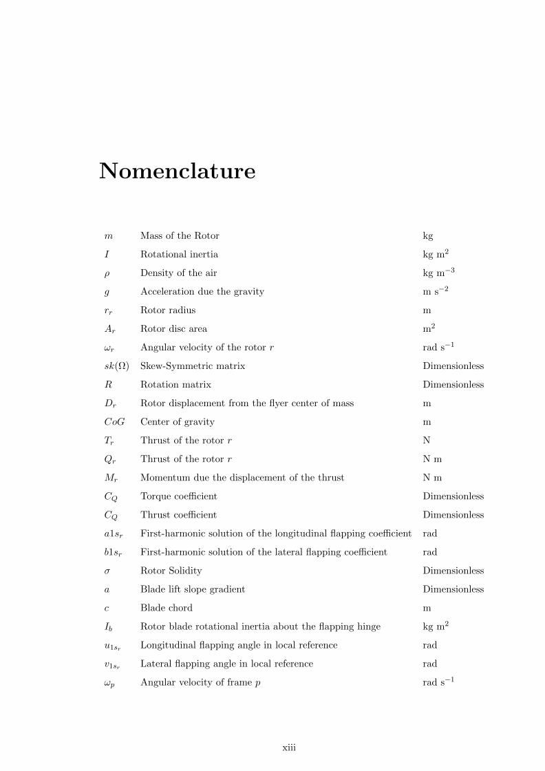
Nomenclature
m Mass of the Rotor kg
I Rotational inertia kg m2
ρ Density of the air kg m−3
g Acceleration due the gravity m s−2
rr Rotor radius m
Ar Rotor disc area m2
ωr Angular velocity of the rotor r rad s−1
sk(Ω) Skew-Symmetric matrix Dimensionless
R Rotation matrix Dimensionless
Dr Rotor displacement from the flyer center of mass m
CoG Center of gravity m
Tr Thrust of the rotor r N
Qr Thrust of the rotor r N m
Mr Momentum due the displacement of the thrust N m
CQ Torque coefficient Dimensionless
CQ Thrust coefficient Dimensionless
a1sr First-harmonic solution of the longitudinal flapping coefficient rad
b1sr First-harmonic solution of the lateral flapping coefficient rad
σ Rotor Solidity Dimensionless
a Blade lift slope gradient Dimensionless
c Blade chord m
Ib Rotor blade rotational inertia about the flapping hinge kg m2
u1sr Longitudinal flapping angle in local reference rad
v1sr Lateral flapping angle in local reference rad
ωp Angular velocity of frame p rad s−1
xiii
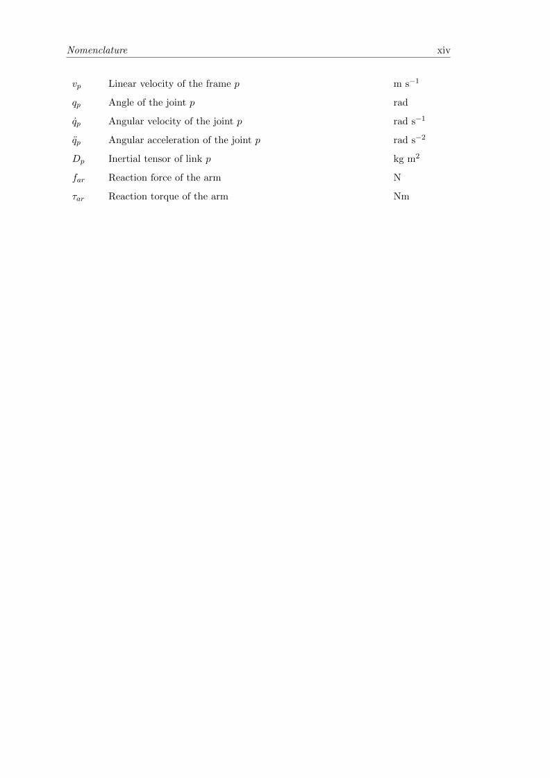
Nomenclature xiv
vp Linear velocity of the frame p m s−1
qp Angle of the joint p rad
qp Angular velocity of the joint p rad s−1
qp Angular acceleration of the joint p rad s−2
Dp Inertial tensor of link p kg m2
far Reaction force of the arm N
τar Reaction torque of the arm Nm
Chapter 1
Introduction
1.1 Motivation
In the last years, there has been an increasing importance of quadrotors in society and
also of the tasks that they can do. There is a need for extending the capabilities of a
quadrotor to satisfy the increasing demand of new services from some companies.
The motivation of this project is to design a Nonlinear Model Predictive Control (NMPC)
for a quadrotor robotic arm attached to its body. Most of the literature reports methods
about how to control an Unmanned Aerial Vehicle (UAV) applying a model predictive
control to a linearized model, like in Bouffard [2012]. Other papers are focused on find-
ing an appropriate mathematical model that explains most of the dynamic effects that
occur during maneuvering tasks well explained in Pounds et al. [2006]. But there are
few papers like Bangura and Mahony [2012] that try to control the quadrotor using a
NMPC algorithm.
The quadrotor in which this research is based on has been described in Sanramaria
and Andrade [2014] and it is used by Institut de Robotica i Informatica Industrial
(CSIC-UPC) (namely here IRI) for research in the Aerial Robotics Cooperative Assem-
bly System ARCAS1 European project. This European project has the goal to design
and develop cooperating flying robots for assembly operations. This quadrotor will have
to be able to cooperate with other robots in order to accomplish different goals like
1http://www.arcas-project.eu/
1
Introduction 2
surveillance, assembly of structures or to track and detect objects. With this thesis a
new approach to control a quadrotor with a robotic arm is going to be presented.
1.2 Objectives
The main goal of this thesis is to use the NMPC strategy to control a quadrotor like in
the existing literature. The new feature added is that the quadrotor has a robotic arm
attached to its body and the NMPC should compensate the perturbations generated
by the motion of this arm. This thesis has the aim of developing a first approach of
a controller able to manage these perturbations. More specific objectives have been
proposed as follows:
1. Designing an algorithm to study the viability of the control strategy (given features
such as complexity, computational burden, etc.).
2. Discretizing and implementing in Matlab environment the dynamic equations of
the quadrotor with the robotic arm.
3. Coupling the dynamic effects of the quadrotor and the arm.
4. Build a real parametrized model of a quadrotor and a robotic arm.
5. Designing an NMPC to control the dynamics and carry the system to specific
operational points.
6. Analysing the behaviour of the quadrotor while it is holding a position and the
arm is in a fixed pose or in movement.
7. Analysing the behaviour of the quadrotor while it is in movement and the arm is
in a fixed pose or in movement.
1.3 Scope of Research
Some decisions have been taken by an heuristic method since the related issues were out
of the scope of this research. The sampling time and the prediction and control horizon
Introduction 3
have been chosen in order to properly run the simulations and verify the tests but in
any case they have been optimized to run the NMPC algorithm at the fastest velocity.
The aim of this project is to design a NMPC for a simulation environment, so the code
is not optimized to be used in real time. Moreover, the identification of the model is out
of the study. During this thesis, parameters chosen to design the model of the quadrotor
and the arm have been mixed from different literature references. However, all the values
selected have been verified to ensure that they were real and possible values. Finally,
the trajectory made by the arm is not determined by the NMPC. Multiple PIs have
been designed to control each joint. Performance and stability of its trajectory are not
taken into account within this study.
1.4 Outline of the Thesis
This thesis is organised as follows:
Chapter 2 - Background: The background contains all the theoretical information
that is necessary to understand implementation and results. At the beginning,
a brief description of the state of the art is presented. Next there is a detailed
explanation about the UAV, the robotic arm and the control algorithm chosen for
this study.
Chapter 3 - Case study description: In Chapter 3, a description of the implemen-
tation is presented. There is a detailed description of the equations that define
both the dynamics of the quadrotor and the robotic arm. There is also a expla-
nation about the parameters that define the model of each device. Finally, the
NMPC designed is presented including all its features.
Chapter 4 - Results: In Chapter 4, the results of the five scenarios tested are pre-
sented. Each section has a brief description of the initial conditions and a sum-
mary with the results obtained. Additionally in this chapter, there is a description
of the perturbations.
Introduction 4
Chapter 5 - Conclusions and Future Work: Conclusions derived from these results
are presented in this Chapter. It is commented the goals achieved and possible is-
sues that happened. Possible improvements are detailed and new interesting lines
of research.
Chapter 2
Background
In this chapter, the three main elements used during this thesis are described:
The first element is an UAV, more specifically a quadrotor. During these times, it is
the most popular vehicle in the commercial field and so the most studied system,
apart from being the cheapest model that can be found. This is perhaps why most
of research laboratories are focusing their studies on this system.
The second element is a robotic arm. This mechanism increases the versatility of the
quadrotor in order to accomplish certain tasks. Currently there are lots of types of
robotics arms. Considering that a quadrotor has a small payload, the arm has to
be light but strong enough to carry the maximum weight possible. So, in that case,
the robotic arm designed by IRI, described in Sanramaria and Andrade [2014], has
been chosen to test the methods explained in this thesis.
The third element is the control algorithm. An NMPC has been selected to control
the whole system. The main reason is because there are several articles identifying
models of quadrotors and it is possible to take advantage of them using controllers
based on models like in Bresciani [2008].
The last section contains a description about the current state of each part. A brief
explanation about the current techniques and technologies existing is presented.
5
Background 6
2.1 Unmanned Aerial Vehicles
UAV is an acronym for Unmanned Aerial Vehicle, which is an aircraft with no
pilot on board. Usually, UAVs are controlled remotely and can fly autonomously
based on either pre-programmed flight or using more complex dynamics.
The UAV concept is becoming more popular each year. There are many types,
sizes and prices of UAVs (see Figure 2.5). The purpose of this thesis is to equip
an arm to a quadrotor and control its dynamics by using an NMPC. The robotic
arm generates a perturbation that the control algorithm has to manage in order
to maintain the system in a fixed position or move the quadrotor to a desired
position. So an UAV with the hover capability is needed in order to hold a fixed
position while an arm is working in some task.
Keeping this in mind, the most used UAVs are based on a system with vertical
thrust. That kind of technology consists in a generation of a vertical force to
compensate the gravity component of the whole dynamic system. It is also possible
by combining the different forces generated to obtain other forces and torques in
all axis to move the robot to any position with a desired motion as it is described
in Pounds et al. [2006].
There are several types of rotor systems as a function of the task that it has to
do. Depending on the autonomy, the payload or maneuverability, the number of
rotors can change between models, for example this eight rotor UAV described in
Romero et al. [2009].
On the other hand, other features that could change drastically the behavior of
the UAV are the propellers as explained in Pounds [2007]. This thesis is based
on a model of four rotors, henceforth named quadrotor. These vehicles are used
to be controlled with an electronic system able to stabilize the aircraft. These
UAVs can be flown indoors as well as outdoors because of their small size and
agile maneuverability. However, if the quadrotor has any variable perturbation,
its performance could drop until being unstable. This is the reason why it is
important to design a control algorithm able to manage these perturbations.
Even in the quadrotor category, there are several types depending on the position
of the rotors relative to its center of mass (X-type, V-type or Stingray-type, see
Figure 2.1). For this thesis, a X-Type has been chosen since its dynamic model
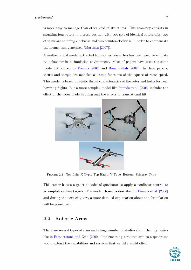
Background 7
is more easy to manage than other kind of structures. This geometry consists in
situating four rotors in a cross position with two sets of identical rotorcrafts, two
of them are spinning clockwise and two counter-clockwise in order to compensate
the momentum generated (Martinez [2007]).
A mathematical model extracted from other researches has been used to emulate
its behaviour in a simulation environment. Most of papers have used the same
model introduced by Pounds [2007] and Bouabdallah [2007]. In these papers,
thrust and torque are modeled as static functions of the square of rotor speed.
This model is based on static thrust characteristics of the rotor and holds for near
hovering flights. But a more complex model like Pounds et al. [2006] includes the
effect of the rotor blade flapping and the effects of translational lift.
Figure 2.1: Top-Left: X-Type. Top-Right: V-Type. Bottom: Stingray-Type
This research uses a generic model of quadrotor to apply a nonlinear control to
accomplish certain targets. The model chosen is described in Pounds et al. [2006]
and during the next chapters, a more detailed explanation about the formulation
will be presented.
2.2 Robotic Arms
There are several types of arms and a huge number of studies about their dynamics
like in Featherstone and Orin [2000]. Implementing a robotic arm to a quadrotor
would extend the capabilities and services that an UAV could offer.
Background 8
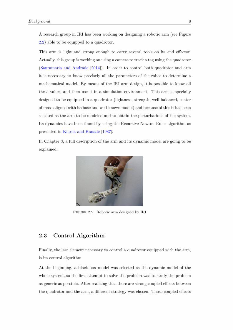
A research group in IRI has been working on designing a robotic arm (see Figure
2.2) able to be equipped to a quadrotor.
This arm is light and strong enough to carry several tools on its end effector.
Actually, this group is working on using a camera to track a tag using the quadrotor
(Sanramaria and Andrade [2014]). In order to control both quadrotor and arm
it is necessary to know precisely all the parameters of the robot to determine a
mathematical model. By means of the IRI arm design, it is possible to know all
these values and then use it in a simulation environment. This arm is specially
designed to be equipped in a quadrotor (lightness, strength, well balanced, center
of mass aligned with its base and well-known model) and because of this it has been
selected as the arm to be modeled and to obtain the perturbations of the system.
Its dynamics have been found by using the Recursive Newton Euler algorithm as
presented in Khosla and Kanade [1987].
In Chapter 3, a full description of the arm and its dynamic model are going to be
explained.
Figure 2.2: Robotic arm designed by IRI
2.3 Control Algorithm
Finally, the last element necessary to control a quadrotor equipped with the arm,
is its control algorithm.
At the beginning, a black-box model was selected as the dynamic model of the
whole system, so the first attempt to solve the problem was to study the problem
as generic as possible. After realizing that there are strong coupled effects between
the quadrotor and the arm, a different strategy was chosen. Those coupled effects
Background 9
prevented from finding a relation between the dynamics of the quadrotor and the
dynamics of the robotic arm.
As the dynamic model of a quadrotor and an arm is well known, a black-box
model could be discarded in order to use parametrized models. Once the model
type was chosen, the whole problem could be solved as an optimization one. Stan-
dard approaches to quadrotor control have been based on linear controller design.
These methods include proportional integral derivative (PID) controllers (Noth
et al. [2004]), linear quadratic regulator (LQR) (Shin et al. [2005]) or robust H∞
(La Civita et al. [2006]). Another method consists in linearizing the model around
a certain working point of the quadrotor and then applying a predictive control
strategy as in Bouffard [2012] and Bresciani [2008].
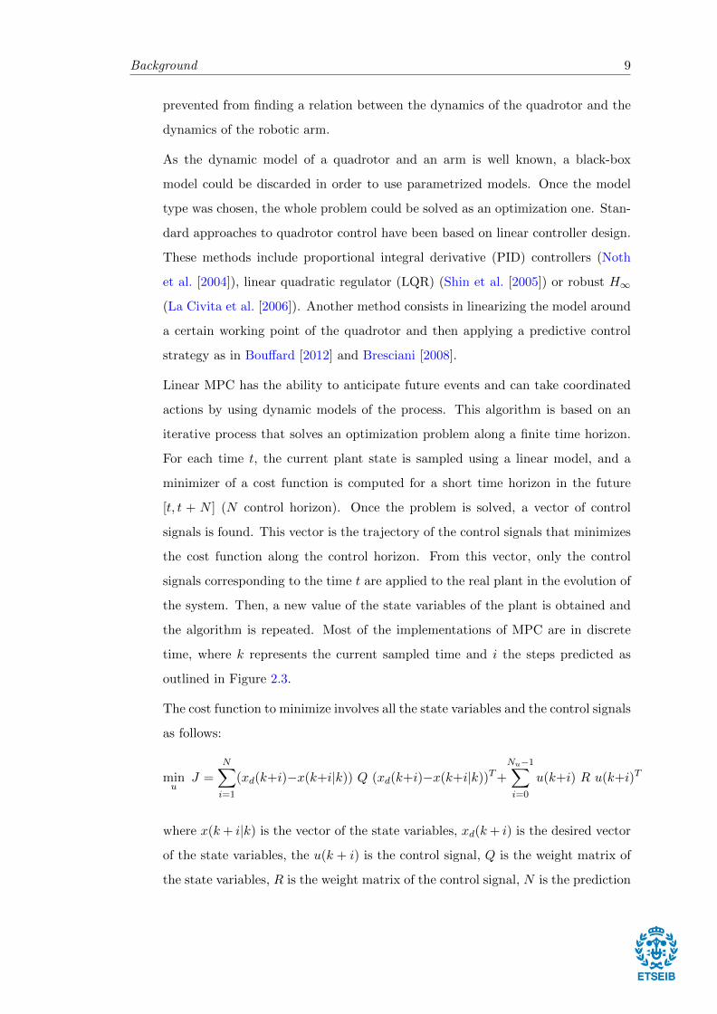
Linear MPC has the ability to anticipate future events and can take coordinated
actions by using dynamic models of the process. This algorithm is based on an
iterative process that solves an optimization problem along a finite time horizon.
For each time t, the current plant state is sampled using a linear model, and a
minimizer of a cost function is computed for a short time horizon in the future
[t, t + N ] (N control horizon). Once the problem is solved, a vector of control
signals is found. This vector is the trajectory of the control signals that minimizes
the cost function along the control horizon. From this vector, only the control
signals corresponding to the time t are applied to the real plant in the evolution of
the system. Then, a new value of the state variables of the plant is obtained and
the algorithm is repeated. Most of the implementations of MPC are in discrete
time, where k represents the current sampled time and i the steps predicted as
outlined in Figure 2.3.
The cost function to minimize involves all the state variables and the control signals
as follows:
minu
J =N∑i=1
(xd(k+i)−x(k+i|k)) Q (xd(k+i)−x(k+i|k))T+
Nu−1∑i=0
u(k+i) R u(k+i)T
where x(k+ i|k) is the vector of the state variables, xd(k+ i) is the desired vector
of the state variables, the u(k + i) is the control signal, Q is the weight matrix of
the state variables, R is the weight matrix of the control signal, N is the prediction
Background 10
Figure 2.3: Scheme of MPC algorithm
horizon length and Nu is the control horizon length. Also, different types of cost
function could be considered to obtain the desired performance.
The minimization of the cost function is subjected constraints defined by the de-
signer in order to determine a state space where the optimization problem should
be solved. To obtain the state variables in a future prediction, a mathematical
model of the plant is needed.
There is a variant of this algorithm for more complex systems called Nonlinear
Model Predictive Control (NMPC). Adding the nonlinear model and nonlinear
constraints improve the response of the system at the expense of increasing the
necessary computational burden.
The numerical solution of the NMPC problem is typically based on direct opti-
mal control methods using Newton-type optimization schemes. NMPC and MPC
algorithms typically take advantage of the fact that consecutive optimal control
problems are similar to each other. This allows to initialize the Newton-type solu-
tion procedure efficiently by a suitable shifted guess from the previously computed
optimal solution, saving considerable amounts of computational time. A scheme
of the global workflow is presented in Figure 2.4.
Plant: System to be controlled. This is the real plant that is going to be con-
trolled. Usually, it is difficult to obtain an appropriate model of its behaviour,

Background 11
Figure 2.4: NMPC scheme
mainly for complex nonlinear systems.
State Estimator: Make a estimation of the state variables. This module allows
to do an estimation of the state of the real plant. Often the algorithm used
need applies sensor fusion to increase accuracy. Its precision is quite impor-
tant to start the NMPC with the correct initial states.
Dynamic Optimizer: Solve the optimal problem. Is the module that solves
the optimal problem by using the system model, the cost function and the
constraints. This module has to evolve the system and find the optimal
control to move the real plant to a desired state.
System Model: Mathematical model of the behavior of the plant. This model is
used to emulate the real plant and evolves the system during the optimization.
Cost Function: Function that should be minimized. This expression codifies the
targets that should accomplish at each time instant. The function can weigh
each objective.
Constraints: Restrictions that should be respected to solve the optimization
problem. It allows to define the performance and it implements the physics
restrictions of the actuators.
The NMPC algorithm has been chosen to control the quadrotor equipped with an
arm. A more detailed explanation is presented in Section 3.3. On the other hand,
the robotic arm has been treated as a dynamic perturbation of the quadrotor, so
there is no need to control its joints. Nevertheless, it is necessary to know the exact
model of the arm to calculate the dynamic reactions applied to the quadrotor due
Background 12
to the motion of the arm during its trajectory. The trajectory of the arm and their
perturbations are calculated before applying the NMPC algorithm, so it turns out
as a parameter of the system. This means that, for each instant time, it is possible
to know the reaction of the arm into the quadrotor.
The main problem of the strategy in a real case is that a suitable and accurate
estimation of the state variables of the quadrotor is necessary. However, this
project is developed in a simulation environment, so it is possible to obtain the
state variables of the plant by using a model of the system. During the next
chapters, a more detailed discussion of the problem will be presented.
2.4 State of the Art
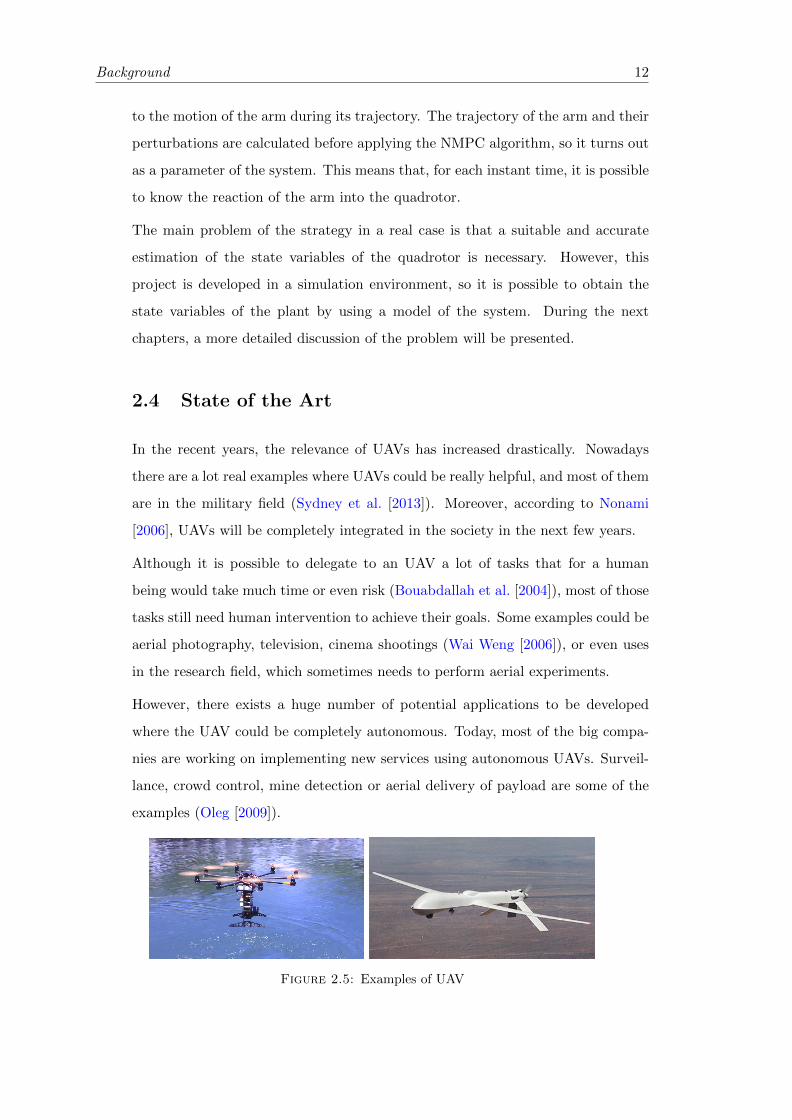
In the recent years, the relevance of UAVs has increased drastically. Nowadays
there are a lot real examples where UAVs could be really helpful, and most of them
are in the military field (Sydney et al. [2013]). Moreover, according to Nonami
[2006], UAVs will be completely integrated in the society in the next few years.
Although it is possible to delegate to an UAV a lot of tasks that for a human
being would take much time or even risk (Bouabdallah et al. [2004]), most of those
tasks still need human intervention to achieve their goals. Some examples could be
aerial photography, television, cinema shootings (Wai Weng [2006]), or even uses
in the research field, which sometimes needs to perform aerial experiments.
However, there exists a huge number of potential applications to be developed
where the UAV could be completely autonomous. Today, most of the big compa-
nies are working on implementing new services using autonomous UAVs. Surveil-
lance, crowd control, mine detection or aerial delivery of payload are some of the
examples (Oleg [2009]).
Figure 2.5: Examples of UAV
Background 13
In order to use autonomous UAVss it is necessary to develop new methods and
algorithms to control these vehicles. The model predictive control methods used in
Raemaekers [2007] or in Grancharova et al. [2012] is one clear example. However,
right now almost all the external perturbations are compensated by a human. In
this way, the final target is to find a method able to understand the situation,
predict what is going to happen and therefore correct the behaviour of the UAV
in order to accomplish the necessary performance to reach the goal.
There are several types of UAVs (see Figure 2.5) and each one reacts differently in
front the perturbations. At the moment, the most integrated and popular UAV in
our society is the quadrotor. This mechanism was conceived in 1907 by Breguet
and Richet as it is described in Leishman [2002]. The first model was a large and
heavy model that could lift only over a small height and for a short duration.
After a lot of research the quadrotor is having people attention and each day its
relevance is increasing for the companies.
In order to model the quadrotor physics, some works such as Belkheiri et al. [2012]
and Zhu and Huo [2010] approximate its dynamics by a linear system, for which
standard linear controllers can be designed. Other authors use nonlinear control
techniques, as for example Mellinger and V. [2011] that used feedback linearization,
Vries and Subbarao [2010] employing backstepping techniques, or Benallegue et al.
[2006] developing sliding mode control. Regarding NMPC methods, some authors
like Bangura and Mahony [2012] have designed a controller to manage the dynamics
of a quadrotor. Other sophisticated projects have even designed a controller with
a model of the wind perturbation like in Alexis et al. [2010].
On the other hand, the use of robotic arms in the society is widespread in several
areas. Some examples can be the use of robotic arms for cooperation tasks as in
Hayati [1986], space as in Fukuda [1985] or even surgery as Velliste et al. [1995]
did. Moreover, there are a lot of studies about how to control and minimize
errors, like in Bicchi and Tonietti [2004], and their dynamics and behaviors are
well known by studies like Herrera et al. [2012]. In this way, it is a good choice to
use robotic arms built on the quadrotors in order to add new features to this flying
machines. By using both robotic structures, new applications could be developed
like collaborative tasks to move objects by pincers, track object with a camera in
the end-effector as it is described in Allen et al. [1993] or anchoring the quadrotors
Background 14
to recharge its batteries. This thesis develops a 6DOF model for a quadrotor that
includes a model of the perturbation of the robotic arm.
Chapter 3
Case Study Description and
Control Problem
In this section, a full description of the dynamic equations of the quadrotor and
its model is done. Also, the Newton-Euler solution for the particular case of
the selected arm is detailed. Finally, the description of the designed NMPC is
presented at the end of this chapter.
3.1 Quadrotor Description
3.1.1 Dynamic Equations of a X-Type Quadrotor
The mathematical model of the quadrotor comes from the description done by
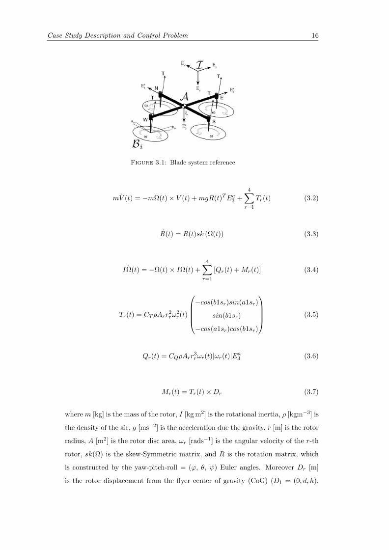
Pounds et al. [2006]. Suppose two frames as in Figure 3.1:
1. Inertial frame: I = Ex, Ey, Ez, where Ez is in the gravity direction.
2. Body frame: A frame located in the body of the quadrotor. Its axis are
denoted by A = Ea1 , Ea2 , Ea3, with center in ξ = xc, yc, zc in meters.
Both frames are related by a rotation matrix R : A→ I We also define V (t) [m/s]
and Ω(t) [rad/s] as the linear and angular velocity of the frame A expressed with
respect to base A.
The dynamic equations of the quadrotor are:
ξ(t) = RV (t) (3.1)
15
Case Study Description and Control Problem 16
Figure 3.1: Blade system reference
mV (t) = −mΩ(t)× V (t) +mgR(t)TEa3 +4∑r=1
Tr(t) (3.2)
R(t) = R(t)sk (Ω(t)) (3.3)
IΩ(t) = −Ω(t)× IΩ(t) +
4∑r=1
[Qr(t) +Mr(t)] (3.4)
Tr(t) = CTρArr2rω
2r (t)
−cos(b1sr)sin(a1sr)
sin(b1sr)
−cos(a1sr)cos(b1sr)
(3.5)
Qr(t) = CQρArr3rωr(t)|ωr(t)|Ea3 (3.6)
Mr(t) = Tr(t)×Dr (3.7)
where m [kg] is the mass of the rotor, I [kg m2] is the rotational inertia, ρ [kgm−3] is
the density of the air, g [ms−2] is the acceleration due the gravity, r [m] is the rotor
radius, A [m2] is the rotor disc area, ωr [rads−1] is the angular velocity of the r-th
rotor, sk(Ω) is the skew-Symmetric matrix, and R is the rotation matrix, which
is constructed by the yaw-pitch-roll = (ϕ, θ, ψ) Euler angles. Moreover Dr [m]
is the rotor displacement from the flyer center of gravity (CoG) (D1 = (0, d, h),
Case Study Description and Control Problem 17
D2 = (0,−d, h), D3 = (d, 0, h) and D4 = (−d, 0, h), with d [m] and h [m] as a
length and height respectively above the CoG of the rotor).
Additionally, Tr [N] is the thrust from the r-th rotor, Qr [Nm] is the torque from the
r-th rotor, Mr [Nm] is the momentum due the displacement of the thrust relative
to the CoG, CT is the dimensionless thrust coefficient, which is an experimental
parameter that could vary slightly, and CQ is dimensionless torque coefficient,
which is another experimental parameter.
Finally, a1sr [rad] is the longitudinal flapping coefficient and b1sr [rad] is the lateral
flapping coefficient. These two parameters are related to the blade flapping effect,
which will be explained a few lines later.
Having said that, it is possible to determine the behavior of any type-X quadrotor
by modifying the above mentioned parameters inside (3.1), (3.2), (3.3), and (3.4).
To clarify the use of all the previous equations, a brief description is presented
next:
• Equation (3.1) relates the linear velocity of the CoG with the inertial frame
and the body frame.
• Equation (3.2) shows that the sum of the forces applied on a quadrotor have
to be proportional to its linear acceleration. The equation is split in three
different components. First, is the force due the Coriolis effect. Second, is
the force because of the gravity. And finally, is the thrust generated by each
rotor.
• Equation (3.3) allows to relate the Euler angles rates to the angular velocity
of the inertial frame.
• Equation (3.4) expresses that the sum of the torques applied have to be pro-
portional to its angular acceleration. As before, the final torque is explained
by three elements. The first one is the torque created by an inertial system
that is rotating around an axis. Secondly, Qr(t) corresponds to the torque
generated by each rotor due its angular velocity. Finally, Mr(t) is the mo-
mentum created by the difference between the thrust of one of the rotors and
the thrust generated by the opposite rotor.
• Equation (3.5) is generated by the angular velocity of the rotor. It depends
on the geometry of the propellers and the density of the air, and is multiplied

Case Study Description and Control Problem 18
by a vector that modifies the final direction of the thrust. Instead of a vertical
direction, it appears a component on Ea1 and Ea2 due to the flapping blade
effect (see (3.8), (3.9) and (3.10)).
• Equation (3.6) is the torque generated by a mass (propeller) rotating around
an axis (rotor).
• Equation (3.7) is generated because the thrust is not applied in the CoG and
therefore a torque appears in the frame of the quadrotor.
The quadrotor can move in the three axis by combining the thrust and the torque
of each rotor:
Move forward-backward: To move forward or backward it is necessary to make
a difference between the thrust generated by the front rotor and the back
rotor as it is represented in Figure 3.2. By this process, the∑4
r=1Mr(t) is
not zero so the quadrotor has a slight torque that rotates the system until
the forces and torques are balanced again. A pitch angle is then generated,
which changes the direction of the thrust. A new component of force appears
towards E1a axis that allows an acceleration and therefore a velocity.
Figure 3.2: Forward-Backward movement
Move left-right: As it is shown in Figure 3.3, in order to accomplish these move-
ments, it is necessary to create a difference between the thrust generated by
the lateral rotors. With the same concept explained before, a new torque is
generated and the quadrotor bends a roll angle. Finally the thrust is split in
a vertical component and in a component in the E2a axis.
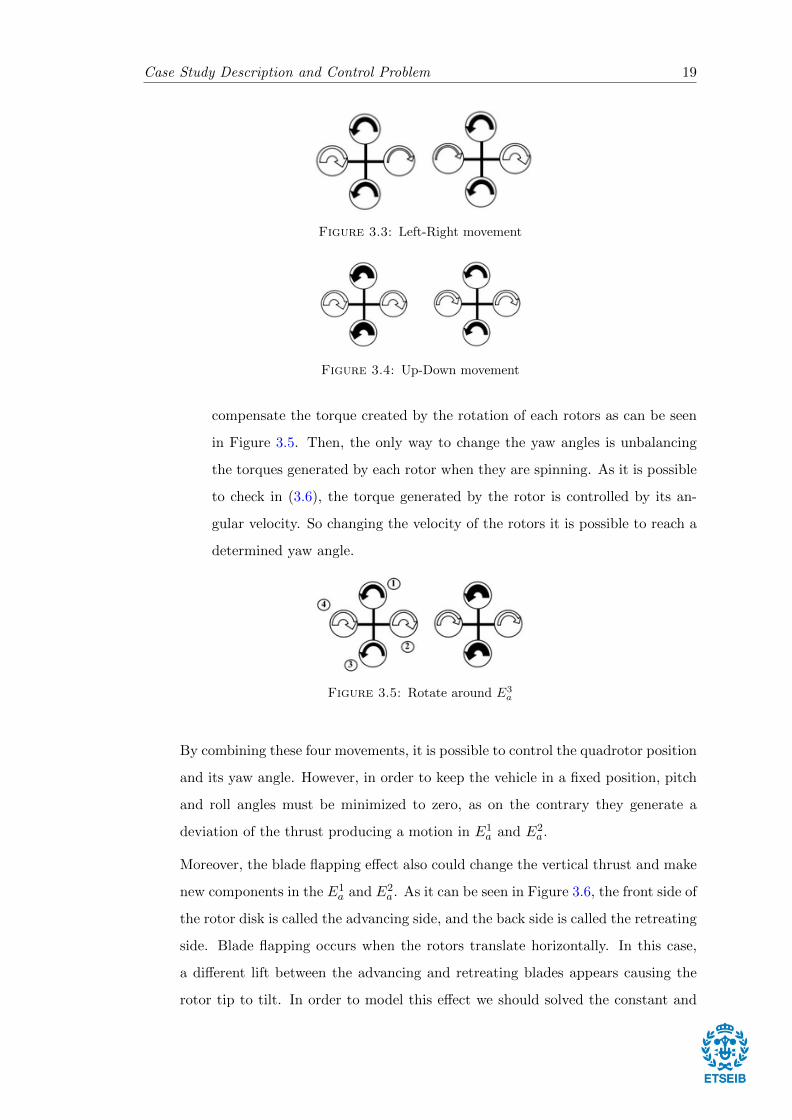
Move up-down: This movemente is described in Figure 3.4. To move up or down
it is necessary that the sum of all vertical thrusts component is more (up) or
less (down) than the gravity force.
Rotate around E3a (yaw motion): To rotate around the E3
a it should exist a
torque around this axis. In a quadrotor, there are two motors that are rotat-
ing clockwise and two motors that are rotating counterclockwise in order to
Case Study Description and Control Problem 19
Figure 3.3: Left-Right movement
Figure 3.4: Up-Down movement
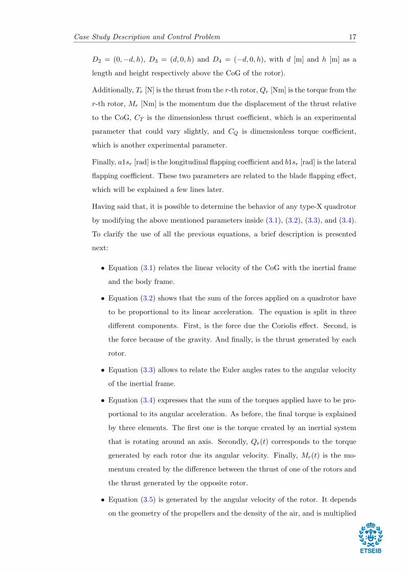
compensate the torque created by the rotation of each rotors as can be seen
in Figure 3.5. Then, the only way to change the yaw angles is unbalancing
the torques generated by each rotor when they are spinning. As it is possible
to check in (3.6), the torque generated by the rotor is controlled by its an-
gular velocity. So changing the velocity of the rotors it is possible to reach a
determined yaw angle.
Figure 3.5: Rotate around E3a
By combining these four movements, it is possible to control the quadrotor position
and its yaw angle. However, in order to keep the vehicle in a fixed position, pitch
and roll angles must be minimized to zero, as on the contrary they generate a
deviation of the thrust producing a motion in E1a and E2
a.
Moreover, the blade flapping effect also could change the vertical thrust and make
new components in the E1a and E2
a. As it can be seen in Figure 3.6, the front side of
the rotor disk is called the advancing side, and the back side is called the retreating
side. Blade flapping occurs when the rotors translate horizontally. In this case,
a different lift between the advancing and retreating blades appears causing the
rotor tip to tilt. In order to model this effect we should solved the constant and
Case Study Description and Control Problem 20
sinusoidal components of the blade centrifugal aerodynamic weight so that find
the tilt angle of the blade as it is explained in (Hussein [2008]).
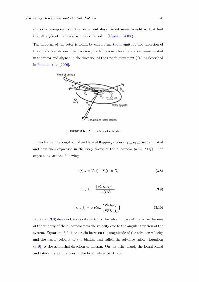
The flapping of the rotor is found by calculating the magnitude and direction of
the rotor’s translation. It is necessary to define a new local reference frame located
in the rotor and aligned in the direction of the rotor’s movement (Br) as described
in Pounds et al. [2006].
Figure 3.6: Parameters of a blade
In this frame, the longitudinal and lateral flapping angles (u1sr , v1sr) are calculated
and now then expressed in the body frame of the quadrotor (a1sr, b1sr). The
expressions are the following:
v(t)rr = V (t) + Ω(t)×Dr (3.8)
µrr(t) =‖v(t)rr(1,2)‖ωr(t)R
(3.9)
Ψrr(t) = arctan
(v(t)rr(2)
v(t)rr(1)
)(3.10)
Equation (3.8) denotes the velocity vector of the rotor r. it is calculated as the sum
of the velocity of the quadrotor plus the velocity due to the angular rotation of the
system. Equation (3.9) is the ratio between the magnitude of the advance velocity
and the linear velocity of the blades, and called the advance ratio. Equation
(3.10) is the azimuthal direction of motion. On the other hand, the longitudinal
and lateral flapping angles in the local reference Br are:
Case Study Description and Control Problem 21
u(t)1sr =1
1− µ(t)2rr2
µ(t)2rr(4θr − 2λr) (3.11)
v(t)1sr =1
1 + µ(t)2rr2
4
3
(Ctσ
2
3
µ(t)rrγ
a+ µ(t)rr
)(3.12)
λr =
√CT2
(3.13)
γ =ρacr4rIb
(3.14)
where σ is the rotor solidity which is the ratio between the total blade area and
the total disk area, a is the blade slope gradient, c is the blade chord [m], rr is the
rotor radius [m], Ib is the rotor blade rotational inertia of the flapping hinge [kg m2].
Equation (3.11) is the longitudinal flapping angle. Depends on the parameters of
the blade and the inflow of the rotor. Equation (3.12) is the lateral flapping angle.
Depends on the geometry of the blade, the inflow of the rotor and the Lock Number
which is defined in Pounds et al. [2006]. Equation (3.13) is an approximation of
the inflow’s rotor. Finally, (3.14) is the Lock Number which represents the ratio
between the aerodynamic and the inertial forces on the blade.
All last parameters are related with the geometry of the blades. Once the longi-
tudinal and lateral flapping angles are calculated in the local body frame of the
rotor, are then transformed back into the quadrotor body frame using the frame
mapping:
JABr =
cos(Ψrr) −sin(Ψrr)
sin(Ψrr) cos(Ψrr)
(3.15)
Finally, the influence of the pitch and roll rates are added to the flapping angles,
i.e., a1sr(t)
b1sr(t)
= JABr
u1sr(t)v1sr(t)
+
16γ·Ωx(t)ωr(t)
+Ωy(t)
ωr(t)
1−µ2rr2
−16γ·Ωy(t)
ωr(t)+
Ωx(t)ωr(t)
1−µ2rr2
(3.16)
with Ωx and Ωy as a pitch and roll rates, ωr(t) angular rate of the rotor r-th.
Case Study Description and Control Problem 22
These values represent the effects of the geometry and physic properties of the
propellers. Depending on the model and the blade shape used, the behavior of
the system varies. Also, by modeling this effect, it is possible to correct the
non controlled lateral movement when the quadrotor is in hover mode. Still, the
equations here presented are a mathematical approximation of a blade physics,
where some assumptions have been made, all explained in Johnson [1994] and in
Bangura and Mahony [2012]. Using the equations described in this section, the
behavior of a quadrotor is completely defined.
3.1.2 Dynamic Equations to Simulate the Real Plant
Once the optimization problem behind the NMPC design is solved, the control
signals that minimize the cost function are determined. The framework of this
study is limited to simulation scenarios so it is a model to emulate the real be-
havior for each sampled time, used also to obtain the variable states for the next
optimization step.
It must be noticed that the model used for the controller is different from the
model used to simulate the real plant. For this reason it is possible to set the
NMPC to handle the potential errors and increase its robustness.
Subsequently, the model used to emulate the behavior of the quadrotor with the
arm is a simplification of the real model described in Section 3.1.1. In this case,
all the flapping effects will be removed from the dynamic equations, i.e.,
a1sr = 0
b1sr = 0
which means that (3.5) has been modified as follows:
Tr(t) = CTρAr2ω(t)2r
0
0
−1
(3.17)
Usually, in a real environment, these values are calculated using an estimator
with sensor fusion algorithms (Kis and Lantos [2011]). These techniques give an
Case Study Description and Control Problem 23
estimation of the state variables of the real system which are used to set the
initial conditions of the NMPC algorithm for the next iteration. In Section 3.3.1,
discretization of the model will be explained.
3.1.3 Physical and Geometrical Parameters of the Quadrotor Model
The equations defined in Section 3.1.1 are a parametrization of the behavior of the
system. To obtain a realistic behavior of the quadrotor it is important to adjust
the physical and geometrical parameters to real values. Focused on this aim, most
of them have been taken from the quadrotor used by the researcher group (IRI)
that has motivated this study. This group has been working in a modification of
the Pelican UAV from Ascending Technologies and its parameters can be found in
its datasheet1.
Other parameters used during this thesis come from the studies Bresciani [2008]
and Gruene and Pannek [2011]. Some of them are experimental and the task to
identify them was out of the scope of this research, so they could not be verified.
For this reason, these parameters are taken from other studies that have checked
its authenticity. Those parameters are split in several categories:
1. Physical: Gravity, viscosity and density of the air are defined to compute all
physical equations.
2. Airframe: Its mass and inertial matrix have been defined in this section. Here
it is also explained the horizontal and vertical displacement from the rotors
relative to CoG.
3. Rotor: All parameters about blade geometry and its physics are described
in this category. Here is where all flapping blade effects are determined in
function of the type of blade used by the quadrotor. Also its mass and its
inertial matrix are detailed.
4. Constants: Some constants are precalculated to optimize the code during the
control loop.
By changing the parameters and using the dynamic equations shown in Section
3.1.1, it is possible to simulate the behavior of any type of X-type quadrotor. The
1http://wiki.asctec.de/display/AR/AscTec+Pelican
Case Study Description and Control Problem 24
versatility of this method has allowed us to create an algorithm that is independent
of the quadrotor used for the control tasks.
3.2 Robotic Arm Description
In this section the parameters and physics that define the behavior of the robotic
arm will be detailed.
3.2.1 Dynamic Equations of a Robotic Arm
The aim of this section is to explain the dynamic equations of the robotic arm.
First, it is necessary to explain the parametrization of the arm and then how to
calculate the dynamic reaction on its base.
It is possible to model a robotic arm with serial joints by using the Denavit-
Hartenberg parameters (Abdel-Malek and Othman [1999]). These four variables
(also called DH parameters) define a particular convention about how to attach
the reference frame of the links for a chain of joints. This convention consists
in assigning a coordinate frame to each link. For each joint there is a matrix
transformation that allows changing from one frame to next. Concatenating this
transformation matrix it is possible to relate the end-effector frame with the base
frame. Depending of the type of joint (hinge or sliding), one of the four parameters
is going to be the variable value and the other remain as constants.
The algorithm to select the right frames Sp and to fulfil DH parameters is:
1. The z-axis is in the direction of the joint axis, i.e., the rotation axis or the
displacement axis.
2. The x-axis is the parallel to the common normal xp = zp−1×zp. The direction
of xp axis is from zp−1 to zp.
3. The y-axis is selected to get the coordinated frame that accomplishes the
right-handed rule.
The four parameters are:
dp: Offset along previous z to the common normal. Distancezp−1(Sp−1, zp−1∩xp).
θp: Angle about previous z from old x to new x. Anglezp−1(xp−1, xp).

Case Study Description and Control Problem 25
ap: Length of the common normal. For a revolute joint, it is the radius about
previous z. Distancexp(zp−1 ∩ xp, Sp).
αp: Angle about common normal from the old z to new z. Anglexp(zi−p, zp).
Figure 3.7: Denavit hartenberg parameters
The DH algorithm determines the configuration of the robotic arm and gives an
unambiguous description of the system. Knowing the angles of each joint, it is also
possible to exactly calculate the position and orientation of the end-effector relative
to its base. This information will be important to estimate dynamic reactions into
the base due to the motion of the end-effector. The final goal to be reached is
to obtain these forces and torques in order to couple them to the quadrotor as a
perturbation. The method that selected to get the dynamic equations is Recursive
Newton-Euler (RNE) algorithm applied into a robotic arm as it is explained in
Featherstone and Orin [2000]. RNE algorithm has two steps. The first step allows
to calculate linear and angular velocity of each link by going from the base to the
end-effector. The second step uses these velocities to solve dynamic equations and
so being able to obtain the force and torque of each joint from end-effector to base.
Finally, with this algorithm it is possible to get the reaction in the base due the
motion of the system.
The formulation for the case of revolution joints is:
Case Study Description and Control Problem 26
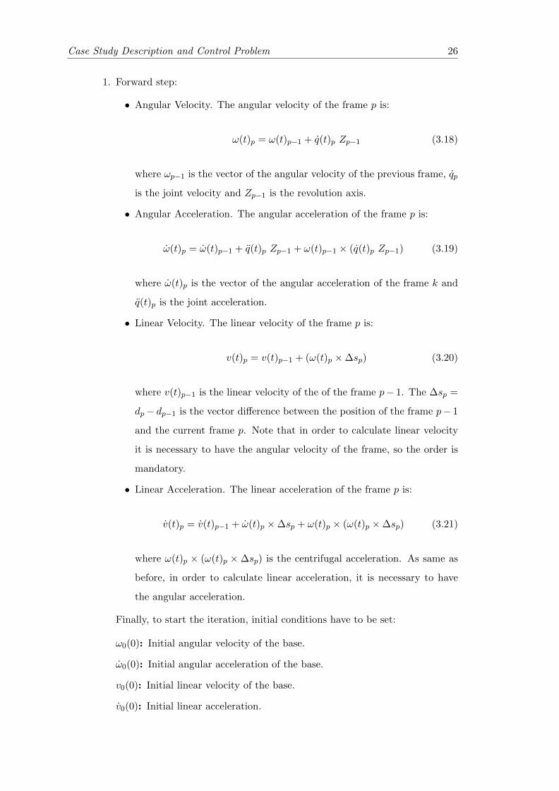
1. Forward step:
• Angular Velocity. The angular velocity of the frame p is:
ω(t)p = ω(t)p−1 + q(t)p Zp−1 (3.18)
where ωp−1 is the vector of the angular velocity of the previous frame, qp
is the joint velocity and Zp−1 is the revolution axis.
• Angular Acceleration. The angular acceleration of the frame p is:
ω(t)p = ω(t)p−1 + q(t)p Zp−1 + ω(t)p−1 × (q(t)p Zp−1) (3.19)
where ω(t)p is the vector of the angular acceleration of the frame k and
q(t)p is the joint acceleration.
• Linear Velocity. The linear velocity of the frame p is:
v(t)p = v(t)p−1 + (ω(t)p ×∆sp) (3.20)
where v(t)p−1 is the linear velocity of the of the frame p− 1. The ∆sp =
dp− dp−1 is the vector difference between the position of the frame p− 1
and the current frame p. Note that in order to calculate linear velocity
it is necessary to have the angular velocity of the frame, so the order is
mandatory.
• Linear Acceleration. The linear acceleration of the frame p is:
v(t)p = v(t)p−1 + ω(t)p ×∆sp + ω(t)p × (ω(t)p ×∆sp) (3.21)
where ω(t)p × (ω(t)p ×∆sp) is the centrifugal acceleration. As same as
before, in order to calculate linear acceleration, it is necessary to have
the angular acceleration.
Finally, to start the iteration, initial conditions have to be set:
ω0(0): Initial angular velocity of the base.
ω0(0): Initial angular acceleration of the base.
v0(0): Initial linear velocity of the base.
v0(0): Initial linear acceleration.
Case Study Description and Control Problem 27
2. Backward step:
• Forces: Define a vector from the end of a link to its CoG, ∆rp = cp − dp
where cp is the location of the center of mass of link p.
The resulting force applied in the CoG is:
f(t)p = f(t)p+1 +mp[v(t)p+ ω(t)p×∆rp+ω(t)p× (ω(t)p×∆rp)] (3.22)
• Torques: First it has to be calculated the moment of the frame p
n(t)p = n(t)p−1 + (∆sp + ∆rp)× f(t)p −∆rp × f(t)p+1 + γ (3.23)
where γ is Dp ω(t)p +ω(t)p× (Dp ω(t)p) with Dp is the inertial tensor of
link p in base space.
Once the moment is solved, the torque is computed as:
τ(t)p = n(t)Tp Zp−1 + bp q(t)p (3.24)
where Zp−1 is the axis of the revolution and bp is the viscous friction
coefficient.
Once the backward step is finished, the forces and torques of each joint are obtained
and RNE algorithm is finished. Reaction force and reaction torque have been
defined as follows:
Reaction force of the arm: The reaction force in the base is the force computed
in the joint 1: far = f(t)1.
Reaction torque of the arm: The reaction torque in the base is the torque
computed in the joint 1: τar = τ(t)1.
These reactions have been coupled in Section 3.3.1.
3.2.2 Dynamic Equations to Simulate the Real Robotic Arm
In order to implement the RNE algorithm using the DH parameters, the Robotics
toolbox from Corke [2011] has been used. This tool allows to use some methods
to calculate the RNE algorithm or the acceleration of each joint given the current
Case Study Description and Control Problem 28
angles of the joints, their velocities and the torques desired. Also, it is possible to
calculate the torque necessary to compensate the gravity effect.
To calculate the dynamic reactions of the base for each sampling time, it is nec-
essary to have the angles, the velocities and the accelerations of each joint. For
the simulation model, a discretized method has been implemented. The method
applied in this thesis to obtain the dynamic reactions is:
1. Calculate the Coriolis velocity using the current angles and velocities of the
joints.
2. To estimate the necessary torque to be applied to each joint to compensate
the effect of the gravity for the current position of the joints.
3. Compute the necessary torque to compensate the centrifugal force due the
Coriolis effect.
4. Solve the direct kinematics using the current angles, velocities and the torques
desired for each joint. This torques contemplate the enough torque to com-
pensate the gravity and Coriolis effect, and also to achieve the motion planned.
After solve it, the accelerations for each joint are obtained.
5. Update the joint velocity using the acceleration and the sampling time.
6. Update the joint angle using the velocity and the sampling time.
7. Finally, using the updated angles, velocities and accelerations, the RNE al-
gorithm is applied. After this step, the base forces and torques reactions are
obtained.
This algorithm is repeated for each sampling time. Due the complexity of the
operations, it is an expensive method that spends a lot of CPU time. Once it is
finished, the result is a vector with three forces and three moments (one per axis)
represented in its base frame. This information will be used during the control
loop as a perturbation of the system.
3.2.3 Physical and Geometrical Parameters of the Arm Model
There are some geometrical and physical parameters that define the dynamic model
of the system. The robotic arm used is designed by IRI on collaboration with
european project Arcas (Sanramaria and Andrade [2014]). This arm is a prototype
Case Study Description and Control Problem 29
and its final design will be slightly different from the model presented in this thesis.
However, the algorithm developed during this thesis are general and can be applied
to any robotic arm. So, even if the arm changes, only by changing the physical
and geometrical parameters the method explained in this study will work properly.
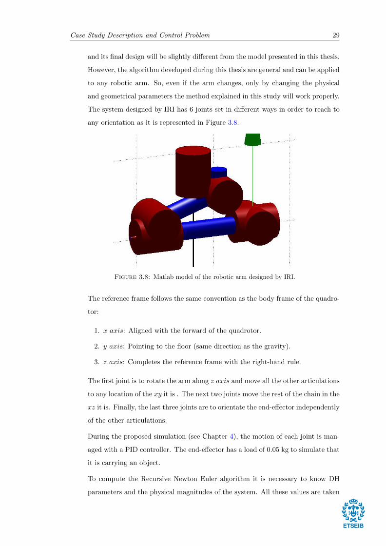
The system designed by IRI has 6 joints set in different ways in order to reach to
any orientation as it is represented in Figure 3.8.
Figure 3.8: Matlab model of the robotic arm designed by IRI.
The reference frame follows the same convention as the body frame of the quadro-
tor:
1. x axis: Aligned with the forward of the quadrotor.
2. y axis: Pointing to the floor (same direction as the gravity).
3. z axis: Completes the reference frame with the right-hand rule.
The first joint is to rotate the arm along z axis and move all the other articulations
to any location of the xy it is . The next two joints move the rest of the chain in the
xz it is. Finally, the last three joints are to orientate the end-effector independently
of the other articulations.
During the proposed simulation (see Chapter 4), the motion of each joint is man-
aged with a PID controller. The end-effector has a load of 0.05 kg to simulate that
it is carrying an object.
To compute the Recursive Newton Euler algorithm it is necessary to know DH
parameters and the physical magnitudes of the system. All these values are taken
Case Study Description and Control Problem 30
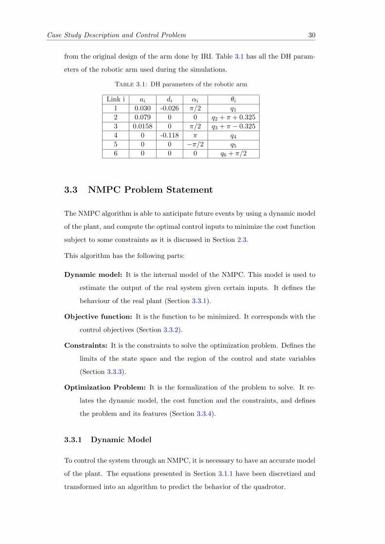
from the original design of the arm done by IRI. Table 3.1 has all the DH param-
eters of the robotic arm used during the simulations.
Table 3.1: DH parameters of the robotic arm
Link i ai di αi θi1 0.030 -0.026 π/2 q12 0.079 0 0 q2 + π + 0.325
3 0.0158 0 π/2 q3 + π − 0.325
4 0 -0.118 π q45 0 0 −π/2 q56 0 0 0 q6 + π/2
3.3 NMPC Problem Statement
The NMPC algorithm is able to anticipate future events by using a dynamic model
of the plant, and compute the optimal control inputs to minimize the cost function
subject to some constraints as it is discussed in Section 2.3.
This algorithm has the following parts:
Dynamic model: It is the internal model of the NMPC. This model is used to
estimate the output of the real system given certain inputs. It defines the
behaviour of the real plant (Section 3.3.1).
Objective function: It is the function to be minimized. It corresponds with the
control objectives (Section 3.3.2).
Constraints: It is the constraints to solve the optimization problem. Defines the
limits of the state space and the region of the control and state variables
(Section 3.3.3).
Optimization Problem: It is the formalization of the problem to solve. It re-
lates the dynamic model, the cost function and the constraints, and defines
the problem and its features (Section 3.3.4).
3.3.1 Dynamic Model
To control the system through an NMPC, it is necessary to have an accurate model
of the plant. The equations presented in Section 3.1.1 have been discretized and
transformed into an algorithm to predict the behavior of the quadrotor.
Case Study Description and Control Problem 31
To define a model, the state variables and the control signals have to be defined:
(x1, x2, x3) = ξ(k) = (xc(k), yc(k), zc(k)): Position relative to the inertial
frame.
(x4, x5, x6) = n(k) = (ψ(k), θ(k), ϕ(k)): Euler angles (yaw, pitch, roll).
(x7, x8, x9) = V (k) = (V (k)x, V (k)y, V (k)z): Linear velocity relative to the
inertial frame.
(x10, x11, x12) = Ω(k) = (Ω(k)x,Ω(k)y,Ω(k)z): Angular velocity of the body
frame.
The control variables are the signals able to control the whole plant and change
its behaviour during the time. In this case, they are the angular rate of the rotors,
i.e.,
(u1, u2, u3, u4) = u(t) = (ω(k)1, ω(k)2, ω(k)3, ω(k)4): Angular rate of each rotor.
Equations (3.1), (3.2) and (3.4) provide the derivative of the position, orientation
and velocities, so in order to compute the state variables in a simulation environ-
ment it is necessary to discretize them. The sampling time is the amount of time
that the time advances for each step of the prediction horizon. If it is too large,
the dynamics of the system will evolve faster than the NMPC could control. On
the other hand, if the sampling time is too short, the future predicted is near of
the current time and the inertia of the motion is not possible to be controlled.
Depending on the control mode, the prediction horizon could vary. These varia-
tions are because the dynamic effects could affect more or less according of the
motion of the quadrotor and then it is necessary a larger or shorter horizon to
stabilize the plant.
The discrete state variables have been obtained as follows:
1. Position:
ξ(k + 1)− ξ(k)
Ts= RV (k) (3.25a)
ξ(k + 1) = (xc, yc, zc)T (k + 1) = (xc, yc, zc)T (k) +RV (k)Ts (3.25b)
Case Study Description and Control Problem 32
2. Linear Velocity:
mV (k + 1)− V (k)
Ts= −mΩ(k)× V (k) +mgR(k)TEa3 +
4∑r=1
Tr(k) (3.26a)
linAcc(k) = −Ω(k)× V (k) + gRTEa3 +1
m
4∑r=1
Tr(k) (3.26b)
V (k + 1) = (Vx, Vy, Vz)(k + 1) = (Vx, Vy, Vz)T (k) + linAcc(k)Ts (3.26c)
where linAcc is the linear acceleration.
3. Euler Angles:
n(k + 1)− n(k)
Ts= W−1Ω(k) (3.27a)
n(k + 1) = (ψ, θ, ϕ)T (k + 1) = (ψ, θ, ϕ)T (k) +W−1Ω(k)Ts (3.27b)
where W−1 is the inverse of the Wronskian. This matrix transforms the Euler
angles rates to angles rates of the inertial frame (See Figure 3.1).
4. Angular Velocity:
IΩ(k + 1)− Ω(k)
Ts= −Ω(k)× IΩ(k) +
4∑r=1
[Qr(k) +Mr(k)] (3.28a)
angAcc(k) = −I−1Ω(k)× IΩ(k) + I−14∑r=1
[Qr(k) +Mr(k)] (3.28b)
Ω(k + 1) = (Ωx,Ωy,Ωz)T (k + 1) = (Ωx,Ωy,Ωz)
T (k) + angAcc(k)Ts (3.28c)
where angAcc is the angular acceleration.
5. Dynamic Equations:
Tr(k) = CTρArr2rω
2r (k)
−cos(b1sr)sin(a1sr)
sin(b1sr)
−cos(a1sr)cos(b1sr)
(3.29a)
Qr(k) = CQρArr3rωr(k)|ωr(k)|Ea3 (3.29b)
Mr(k) = Tr(k)×Dr (3.29c)
The equations (3.29) allow to compute the position of the quadrotor for each sam-
pled time. To couple the quadrotor and arm dynamics, the discretized equations
Case Study Description and Control Problem 33
(3.26) and (3.28) have to be modified:
linAcc(k) = −Ω(k)× V (k) + gR(k)TEa3 +1
m
4∑r=1
[Tr(k)] + Far(k) (3.30a)
angAcc(k) = −I−1Ω(k)× IΩ(k) + I−14∑r=1
[Qr(k) +Mr(k)] + τar(k) (3.30b)
The dynamic effects of the robotic arm are coupled by adding its reaction forces
Far and its reaction torques τar into the equations that compute the accelerations.
In Section 3.2, it is presented a full detailed explanation about how to obtain the
reaction of the forces and torques of the arm. The model is defined by the state
variables as outputs, and the control signals as inputs of the system. By changing
the rotors speed (control signals), it is possible to move the quadrotor to a desired
position and orientation in a determined motion (state variables).
3.3.2 Objective Function
The objective function, also called value function, is the expression that the NMPC
should minimize by looking for the best possible control signals. In this thesis, this
equation expresses the error to a specific state of the system. However, it does
not represent the performance of the trajectory of the state variables. During this
thesis, two different functions have been presented depending on if the quadrotor
has to take off or if it has to reach a position and hold it.
So in this case, the objective function is the minimization of the error of some
state variables. The weights matrix Q allows to prioritize which minimizations
are more important than others. Also this matrix determines which variables are
not going to be minimized. To use the prioritization system, it should be done
the normalization of the variables. By combining (3.34) and considering that the
control signals have not been penalized, it was obtained the cost function used
during the simulation:
J =
N∑i=1
(xd − x(k + i|k)) Q (xd − x(k + i|k))T (3.31)
Notice that the desired vector of state variables is not dependent on the time
because the goal remains constant in all simulated scenarios.
Case Study Description and Control Problem 34
The state variables involved in the objective function are:
(x1, x2, x3, x4, x9) = (xc(k), yc(k), zc(k), ψ(k), Vz(k))
which are the quadrotor position, yaw and velocity in the z axis. On the other
hand, pitch and roll are not included because if the system is forced to have a
determined value of these states, it would imply that the quadrotor will move
along its x or y axis.
As explained in Section 3.1.1, a tilt on its x or y axis generates a change of
the direction of the thrust vector and a component of force could appear in the
horizontal it is. So it is important to let free the pitch and roll in order to allow
the appropriate movement of the quadrotor.
When the system moves along an horizontal axis, it is mandatory to increase the
difference of the rotor speed between the two opposite rotors. By doing this,
the total moment of the system is not compensated and starts to rotate in the
z axis. So it is necessary to fix the desired yaw angle to ensure that the system
orientation is constant. If this restriction is not imposed, it is possible to move
from one position to another but losing the orientation.
Neither linear nor angular velocity have been included since that it is impossible to
hover a quadrotor if the system is not allowed to change its velocity conveniently
(except the Vz(k), which is forced to a value in order to take off). The matrix
weights are:
for m, n = 1, ..., 12
Q(m,m) =
γm,m
xm(ub)−xm(lb)if m = 1, 2, 3, 4, 9
0 otherwise
Q(m,n) = 0
(3.32)
where γm,m is the weight of the state variable xm and xm(ub) − xm(lb) is the range
of the state variable xm that it is used to normalize it. A more detailed description
of the constraints is presented in Section 3.3.3. If the quadrotor has to take off,
γ9,9 6= 0 otherwise γ9,9 = 0.
Case Study Description and Control Problem 35
The NMPC uses (3.32) in order to find the optimal control signals and approach
the system to its goals.
3.3.3 Constraints
The constraints define the state space of the problem. It is a polyhedric space
where the NMPC has to find the optimal solution.
The bigger the space, the larger the search. So it is important to limit each variable
with an upper and lower value. Also, if there is any linear or nonlinear relation
between variables, it should be implemented as a constraints.
The constraints limit all possible solutions to a set of them. Also, those constraints
allow to define the performance desired to accomplish its targets. During this
thesis, the constraints have been categorized in two types:
1. Constraints of the State Variables: All the constraints related to the state
variables are defined in this category. The upper and lower values have to be
defined for the 12 state variables of the plant.
• Position Bounds: It defines the spatial volume allowed to move the
quadrotor:
(x1ub, x2ub, x3ub) = (xcmax, ycmax, z
cmax)
(x1lb, x2lb, x3lb) = (xcmin, ycmin, z
cmin)
The trajectory of the quadrotor has to stay inside this volume in order
to find a solution of the problem. Also, this volume has to be at least big
enough to contain the possible error obtained during the hover maneuver.
• Euler Angles Bounds: It defines the maximum and minimum Euler angles
allowed:
(x4ub, x5ub, x6ub) = (ψmax, θmax, ϕmax)
(x4lb, x5lb, x6lb) = (ψmin, θmin, ϕmin)
Taking into account that the x4 = ψ is the yaw angle, the range of this
variable has to be wide enough to contain all the possible orientations in
the xy it is necessary to accomplish the targets of the quadrotor.
Case Study Description and Control Problem 36
On the other hand, the range of pitch (x5 = θ) and roll (x6 = ϕ) angles
have to be small enough to permit a slight tilt that allows to move the
quadrotor but without losing the control of the plant. For large values of
pitch or roll, the system can rotate completely until the thrust points to
the same direction as the gravity, which would be critical for the plant.
To avoid this, a small range has been chosen.
• Linear Velocity Bounds: It defines the maximum and minimum linear
velocity allowed. These are referenced to the inertial frame:
(x7ub, x8ub, x9ub) = (Vxmax, Vymax, Vzmax)
(x7lb, x8lb, x9lb) = (Vxmin, Vymin, Vzmin)
Those constraints allow to smooth the behaviour of the quadrotor. Due
the limit of its speed, the effect of its dynamics is less aggressive than for
high speeds.
• Angular Velocity Bounds: Defines the range of the angular velocity of
the quadrotor.
(x10ub, x11ub, x12ub) = (Ωxmax,Ωymax,Ωzmax)
(x10lb, x11lb, x12lb) = (Ωxmin,Ωymin,Ωzmin)
As before, it is important to define a narrow range of values in order to
do not lose the control of the motion and avoid the possible problems
with the dynamic effects.
2. Constraints of the Control Signals: The constraints of the control signals
usually depend on the physical capabilities of the actuators. In this thesis,
the control signals are the angular rate of the rotors. So depending on the
type of motor used, their limits and their behaviours could change.
The constraints are:
• Angular Rates of the Rotors: It defines the range of the angular velocity
of each rotor. The upper bound corresponds to the maximum possible
angular rate that the motor is able to rotate.
Case Study Description and Control Problem 37
These constraints take into account the sign of the value because the
velocity could be positive or negative depending on whether it turns
clockwise or counter-clockwise:
u1ub = ω1max > 0
u2ub = ω2max < 0
u3ub = ω3max > 0
u4ub = ω4max < 0
On the other hand, the lower bound is the minimum value experimentally
found to avoid losing the control of the system. Under this limit, the
quadrotor may fall down. So actually is not the minimum angular speed
of the rotors:
u1lb = ω1min > 0
u2lb = ω2min < 0
u3lb = ω3min > 0
u4lb = ω4min < 0
So:
ω1min < u1 < ω1max
ω2min < u2 < ω2max
ω3min < u3 < ω3max
ω4min < u4 < ω4max
• Angular Accelerations of the Rotors: It defines the range of the angular
acceleration for each rotor. It is important to define the maximum possi-
ble acceleration because this constraint limits how fast could change the
angular speed of the rotors. For wide ranges, the maneuvers are faster but
also more aggressive so the system could become uncontrolled. On the
other hand, for a narrow ranges, change the state variables of the plant
could be too slow and then it may be difficult to accomplish its goals.
Case Study Description and Control Problem 38
The maximum width of the ranges are determined by the physical prop-
erties of the rotor. To implement this restriction it is necessary to know
the last angular rate of the rotor and compute the current increment:
∆ur(k) = ur(k+i)−ur(k+i−1) < ∆umax → ur(k+i) < ∆umax+ur(k+i−1)
−∆ur(k+i) = −ur(k+i)+ur(k+i−1) < ∆umax → −ur(k+i) < ∆umax−ur(k+i−1)
where ∆umax is the maximum increment of speed allowed for r ∈ [1,4].
Once all those constraints are applied, the states space of the system is
defined and the optimizer can find the solution in the control space.
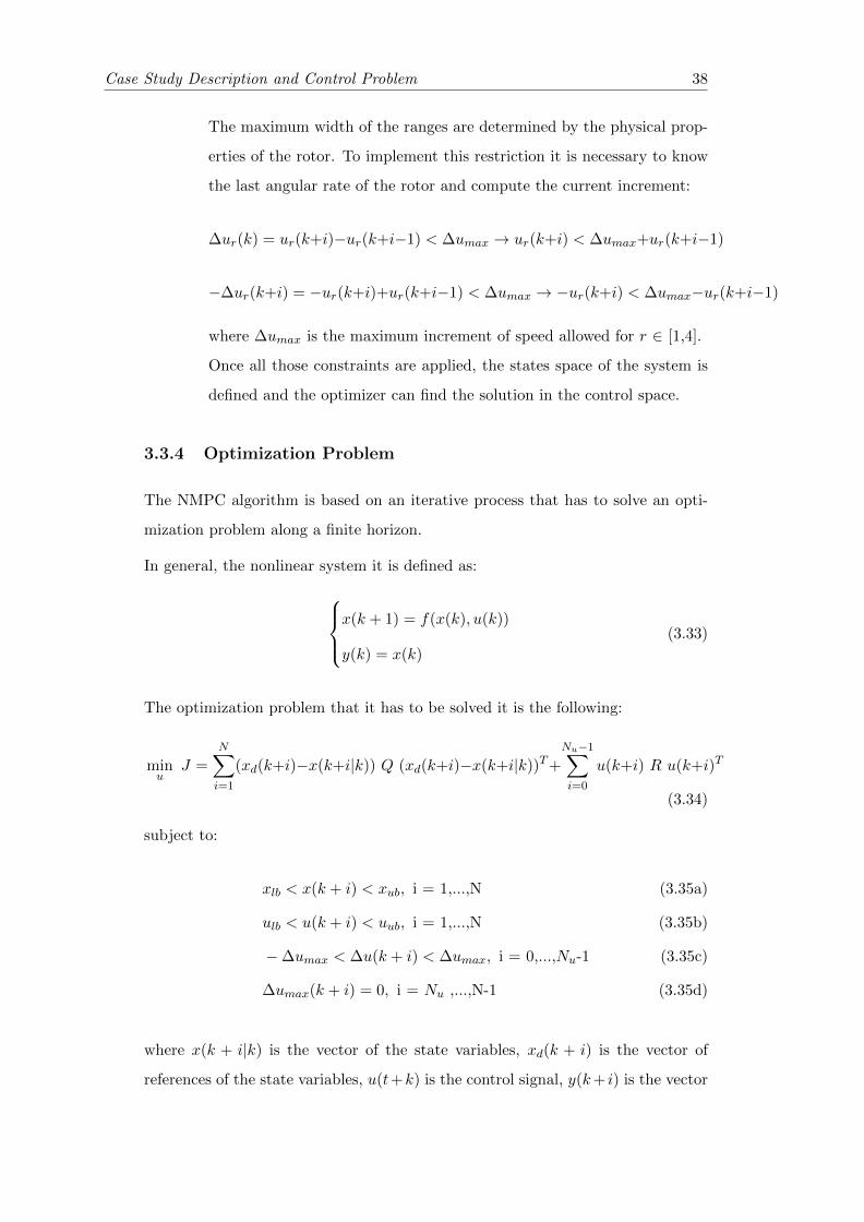
3.3.4 Optimization Problem
The NMPC algorithm is based on an iterative process that has to solve an opti-
mization problem along a finite horizon.
In general, the nonlinear system it is defined as:
x(k + 1) = f(x(k), u(k))
y(k) = x(k)
(3.33)
The optimization problem that it has to be solved it is the following:
minu
J =
N∑i=1
(xd(k+i)−x(k+i|k)) Q (xd(k+i)−x(k+i|k))T+
Nu−1∑i=0
u(k+i) R u(k+i)T
(3.34)
subject to:
xlb < x(k + i) < xub, i = 1,...,N (3.35a)
ulb < u(k + i) < uub, i = 1,...,N (3.35b)
−∆umax < ∆u(k + i) < ∆umax, i = 0,...,Nu-1 (3.35c)
∆umax(k + i) = 0, i = Nu ,...,N-1 (3.35d)
where x(k + i|k) is the vector of the state variables, xd(k + i) is the vector of
references of the state variables, u(t+k) is the control signal, y(k+ i) is the vector
Case Study Description and Control Problem 39
of measurements, Q is the weight matrix of the state variables, R is the weight
matrix of the control signals, N is the prediction horizon length and Nu is the
control horizon length. Moreover ylb, yub, ulb, uub and ∆umax are the constraints
of the problem (more information in Section 3.3.3).
In order to control the plant and bring it to a desired state, it is important to
choose an appropriate control horizon. To simplify the algorithm, the length of the
prediction horizon and the length of the control horizon are the same (N = Nu).
The horizon is the number of steps that the NMPC evolves the system toward
the future to find the optimal control taking into account the future predictions.
As the horizon increases, the complexity to solve the problem also increases, and
the CPU time required increases dramatically. So the power of CPU limits the
horizon. If the control horizon is not large enough the dynamics of the system can
not be predicted properly and then the control could be impossible.
The dynamic model has been defined in Section 3.3.1, the objective function has
been presented in Section 3.3.2 and the constraints have been detailed in Section
3.3.3.

Chapter 4
Simulation Results
Some assumptions have been stated in order to proceed with the simulations and
validate the results:
Computational resources: It has supposed that the processor is powerful enough
to compute all the operations in real time.
Accurate estimator of the state variables: It has assumed that there are a
suitable filter that returns an appropriate estimation of the 12 state variables.
During these tests, this filter has been emulated by using a mathematical
model of the quadrotor.
Point of application: It has assumed that the point of application of the forces
and torques from the arm is the origin of the body frame.
Control the angular rate of the rotors: It has supposed that it is possible to
control the speed of the rotors. It has also assumed that their dynamics are
instant.
Controlled environment: It has supposed a controlled environment, which means
no extra perturbations.
The sampling time is constant: The frame rate of the loops has assumed con-
stant.
Five scenarios have been prepared to test the algorithm developed during the
thesis:
1. The quadrotor takes off and flies until achieves to a specific altitude. The
arm remains in a fixed position.
41
Simulation Results 42
2. Both the quadrotor and the robotic arm remain in a fixed position. The aim
of this test is to try if the system is able to keep a fixed position while its
center of mass has changed.
3. The quadrotor remains in a fixed position and the robotic arm moves toward
a target position. This scenario is a demonstration about how the NMPC
compensates the dynamics of the arm due its motion.
4. The quadrotor moves toward a location and the robotic arm remains in a
fixed position. The aim of this test is to show how the quadrotor can move
to a specific location while it is carrying an object that changes its center of
mass.
5. The quadrotor moves toward a location and the robotic arm moves toward
a target position. This situation has been prepared to check whether the
NMPC is able to predict the perturbations of the arm while the quadrotor
moves towards a space position.
During the next sections, a comparison between those modes is going to be pre-
sented. In order to obtain the perturbation of the arm, it is necessary to simulate
a motion of the arm. For these tests, the same motion is going to be applied in
order to better understand the different behavior of the whole system. The arm
could remain in a fixed position or move toward a specific pose. Each case has
different reaction forces and torques.
Remains in a Fixed Position: The plot showed in Figure 4.1 shows the reac-
tion when the robotic arm remainsin a fixed position. The forces and torques
are constant during all the simulation. Actually, the only remarkable force
that is acting over the system is the force in the z axis, which corresponds to
the force due to the gravity. Also, there is a slight moment in the y axis due
the CoG of the arm is slightly displaced along this axis.
Moves to a Target Position: The movement consists in a small step of 0.2 rad
in all the joints at the same time. The Figure 4.2 shows the reference of
the movement and the trajectory of each joint. Figure 4.3 shows the forces
that the quadrotor will receive when the robotic arm moves. Those dynamics
have to be controlled in order to achieve a steady state. The movement of
the robotic arm starts after 3.4 seconds from the beginning of the simulation.
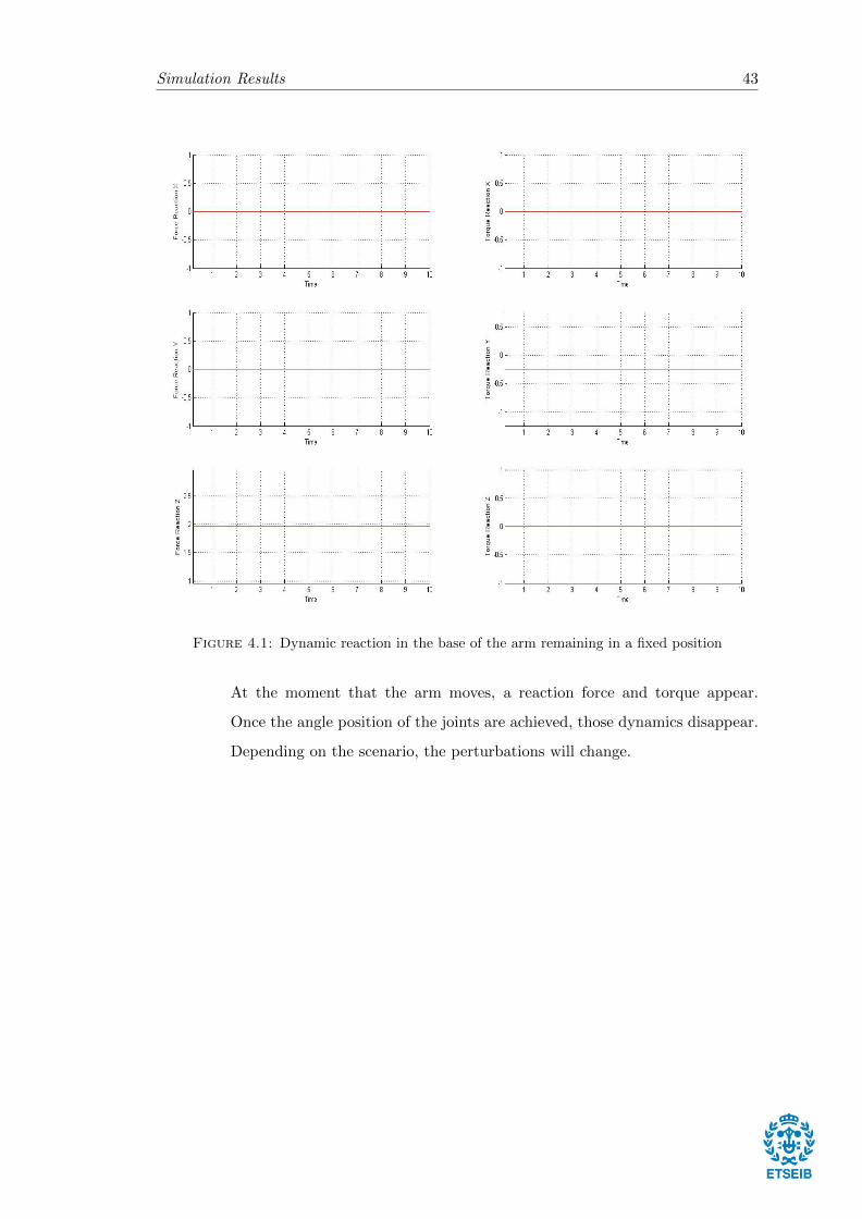
Simulation Results 43
Figure 4.1: Dynamic reaction in the base of the arm remaining in a fixed position
At the moment that the arm moves, a reaction force and torque appear.
Once the angle position of the joints are achieved, those dynamics disappear.
Depending on the scenario, the perturbations will change.
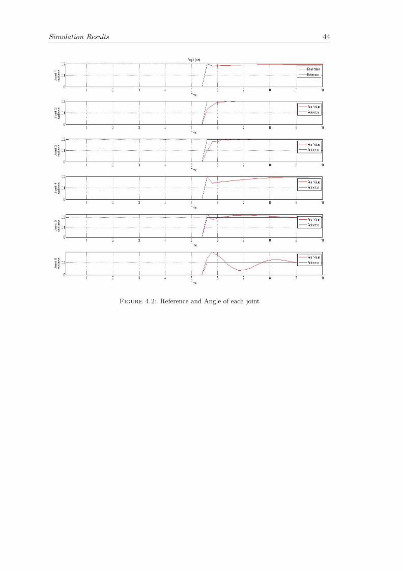
Simulation Results 44
Figure 4.2: Reference and Angle of each joint
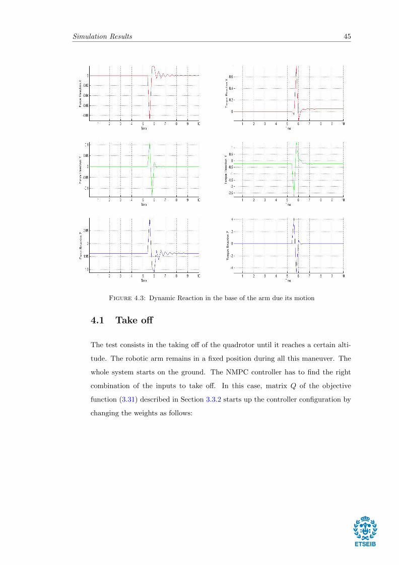
Simulation Results 45
Figure 4.3: Dynamic Reaction in the base of the arm due its motion
4.1 Take off
The test consists in the taking off of the quadrotor until it reaches a certain alti-
tude. The robotic arm remains in a fixed position during all this maneuver. The
whole system starts on the ground. The NMPC controller has to find the right
combination of the inputs to take off. In this case, matrix Q of the objective
function (3.31) described in Section 3.3.2 starts up the controller configuration by
changing the weights as follows:
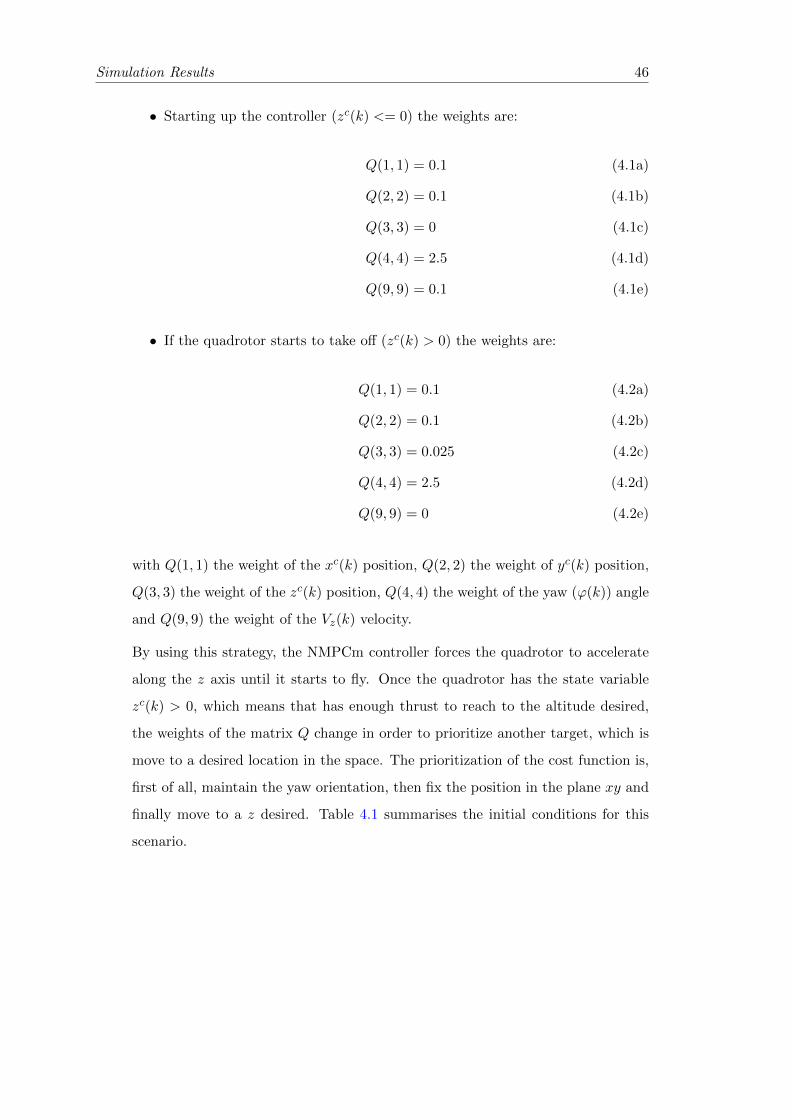
Simulation Results 46
• Starting up the controller (zc(k) <= 0) the weights are:
Q(1, 1) = 0.1 (4.1a)
Q(2, 2) = 0.1 (4.1b)
Q(3, 3) = 0 (4.1c)
Q(4, 4) = 2.5 (4.1d)
Q(9, 9) = 0.1 (4.1e)
• If the quadrotor starts to take off (zc(k) > 0) the weights are:
Q(1, 1) = 0.1 (4.2a)
Q(2, 2) = 0.1 (4.2b)
Q(3, 3) = 0.025 (4.2c)
Q(4, 4) = 2.5 (4.2d)
Q(9, 9) = 0 (4.2e)
with Q(1, 1) the weight of the xc(k) position, Q(2, 2) the weight of yc(k) position,
Q(3, 3) the weight of the zc(k) position, Q(4, 4) the weight of the yaw (ϕ(k)) angle
and Q(9, 9) the weight of the Vz(k) velocity.
By using this strategy, the NMPCm controller forces the quadrotor to accelerate
along the z axis until it starts to fly. Once the quadrotor has the state variable
zc(k) > 0, which means that has enough thrust to reach to the altitude desired,
the weights of the matrix Q change in order to prioritize another target, which is
move to a desired location in the space. The prioritization of the cost function is,
first of all, maintain the yaw orientation, then fix the position in the plane xy and
finally move to a z desired. Table 4.1 summarises the initial conditions for this
scenario.
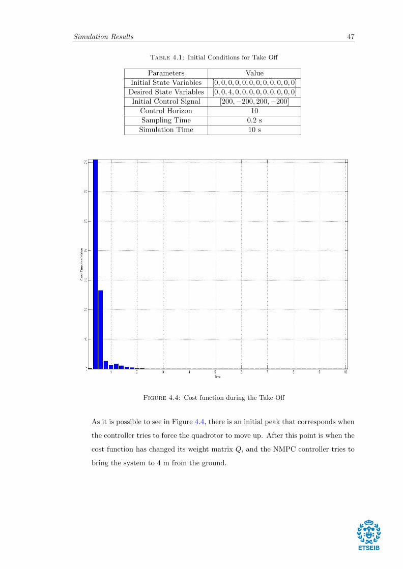
Simulation Results 47
Table 4.1: Initial Conditions for Take Off
Parameters Value
Initial State Variables [0, 0, 0, 0, 0, 0, 0, 0, 0, 0, 0, 0]
Desired State Variables [0, 0, 4, 0, 0, 0, 0, 0, 0, 0, 0, 0]
Initial Control Signal [200,−200, 200,−200]
Control Horizon 10
Sampling Time 0.2 s
Simulation Time 10 s
Figure 4.4: Cost function during the Take Off
As it is possible to see in Figure 4.4, there is an initial peak that corresponds when
the controller tries to force the quadrotor to move up. After this point is when the
cost function has changed its weight matrix Q, and the NMPC controller tries to
bring the system to 4 m from the ground.
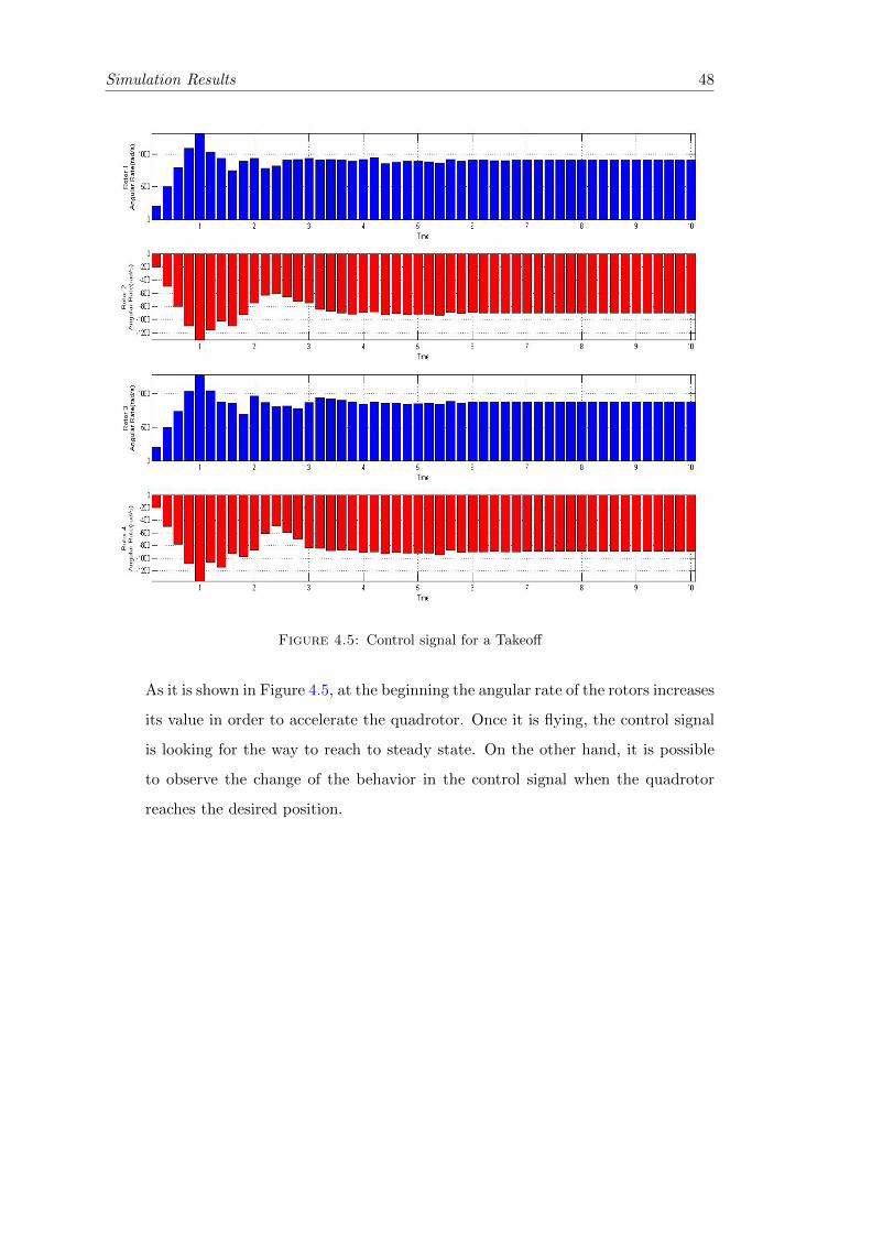
Simulation Results 48
Figure 4.5: Control signal for a Takeoff
As it is shown in Figure 4.5, at the beginning the angular rate of the rotors increases
its value in order to accelerate the quadrotor. Once it is flying, the control signal
is looking for the way to reach to steady state. On the other hand, it is possible
to observe the change of the behavior in the control signal when the quadrotor
reaches the desired position.
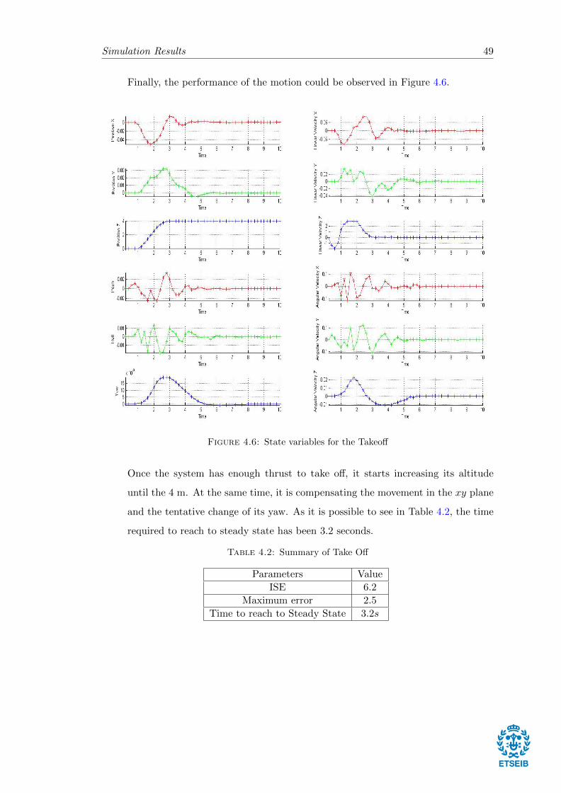
Simulation Results 49
Finally, the performance of the motion could be observed in Figure 4.6.
Figure 4.6: State variables for the Takeoff
Once the system has enough thrust to take off, it starts increasing its altitude
until the 4 m. At the same time, it is compensating the movement in the xy plane
and the tentative change of its yaw. As it is possible to see in Table 4.2, the time
required to reach to steady state has been 3.2 seconds.
Table 4.2: Summary of Take Off
Parameters Value
ISE 6.2
Maximum error 2.5
Time to reach to Steady State 3.2s
Simulation Results 50
4.2 Quadrotor in a fixed position
Table 4.3 contains all the infromation about the initial conditions of the tests.
The aim of this section is to try to stabilize the quadrotor in a fixed position and
orientation in the space. The position desired is (xc(k), yc(k), zc(k) = (0, 0, 4),
while the orientation desired is (ϕ(k) = 0).
During these scenarios, the matrix weights are:
Q(1, 1) = 0.1 (4.3a)
Q(2, 2) = 0.1 (4.3b)
Q(3, 3) = 0.025 (4.3c)
Q(4, 4) = 2.5 (4.3d)
Q(9, 9) = 0 (4.3e)
These weights assure that the quadrotor will stay near the position (0, 0, 4) with a
fixed orientation. At the beginning, the rotors start with an initial angular speed
(900,−900, 900,−900) rad s−1. Those are the necessary velocities to avoid that
the system falls.
Table 4.3: Initial Conditions for Static Control
Parameters Value
Initial State Variables [0, 0, 4, 0, 0, 0, 0, 0, 0, 0, 0, 0]
Desired State Variables [0, 0, 4, 0, 0, 0, 0, 0, 0, 0, 0, 0]
Initial Control Signal [900,−900, 900,−900]
Control Horizon 10
Sampling Time 0.2 s
Simulation Time 10 s
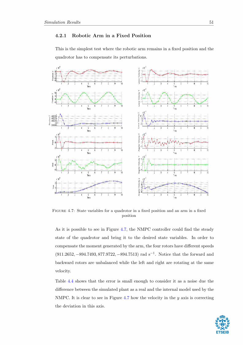
Simulation Results 51
4.2.1 Robotic Arm in a Fixed Position
This is the simplest test where the robotic arm remains in a fixed position and the
quadrotor has to compensate its perturbations.
Figure 4.7: State variables for a quadrotor in a fixed position and an arm in a fixedposition
As it is possible to see in Figure 4.7, the NMPC controller could find the steady
state of the quadrotor and bring it to the desired state variables. In order to
compensate the moment generated by the arm, the four rotors have different speeds
(911.2652,−894.7493, 877.9722,−894.7513) rad s−1. Notice that the forward and
backward rotors are unbalanced while the left and right are rotating at the same
velocity.
Table 4.4 shows that the error is small enough to consider it as a noise due the
difference between the simulated plant as a real and the internal model used by the
NMPC. It is clear to see in Figure 4.7 how the velocity in the y axis is correcting
the deviation in this axis.
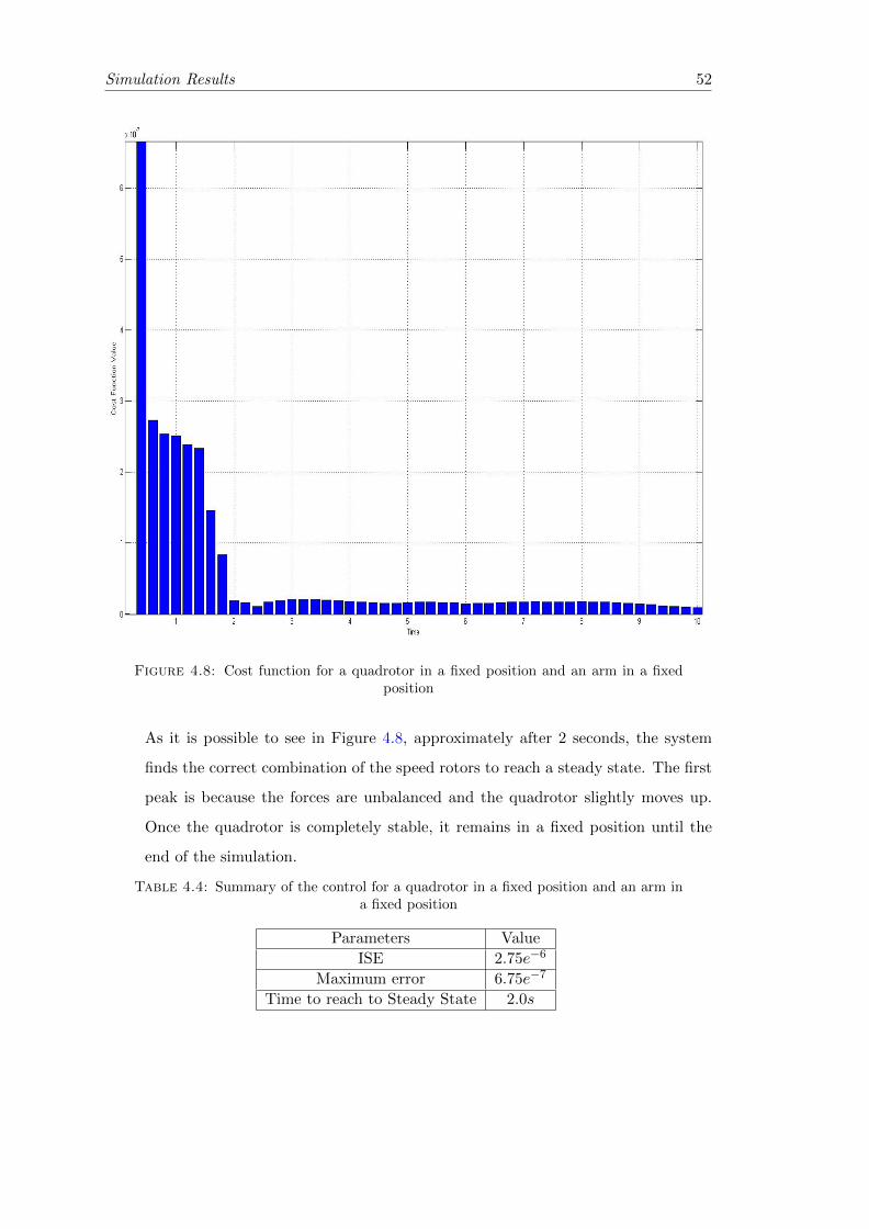
Simulation Results 52
Figure 4.8: Cost function for a quadrotor in a fixed position and an arm in a fixedposition
As it is possible to see in Figure 4.8, approximately after 2 seconds, the system
finds the correct combination of the speed rotors to reach a steady state. The first
peak is because the forces are unbalanced and the quadrotor slightly moves up.
Once the quadrotor is completely stable, it remains in a fixed position until the
end of the simulation.
Table 4.4: Summary of the control for a quadrotor in a fixed position and an arm ina fixed position
Parameters Value
ISE 2.75e−6
Maximum error 6.75e−7
Time to reach to Steady State 2.0s
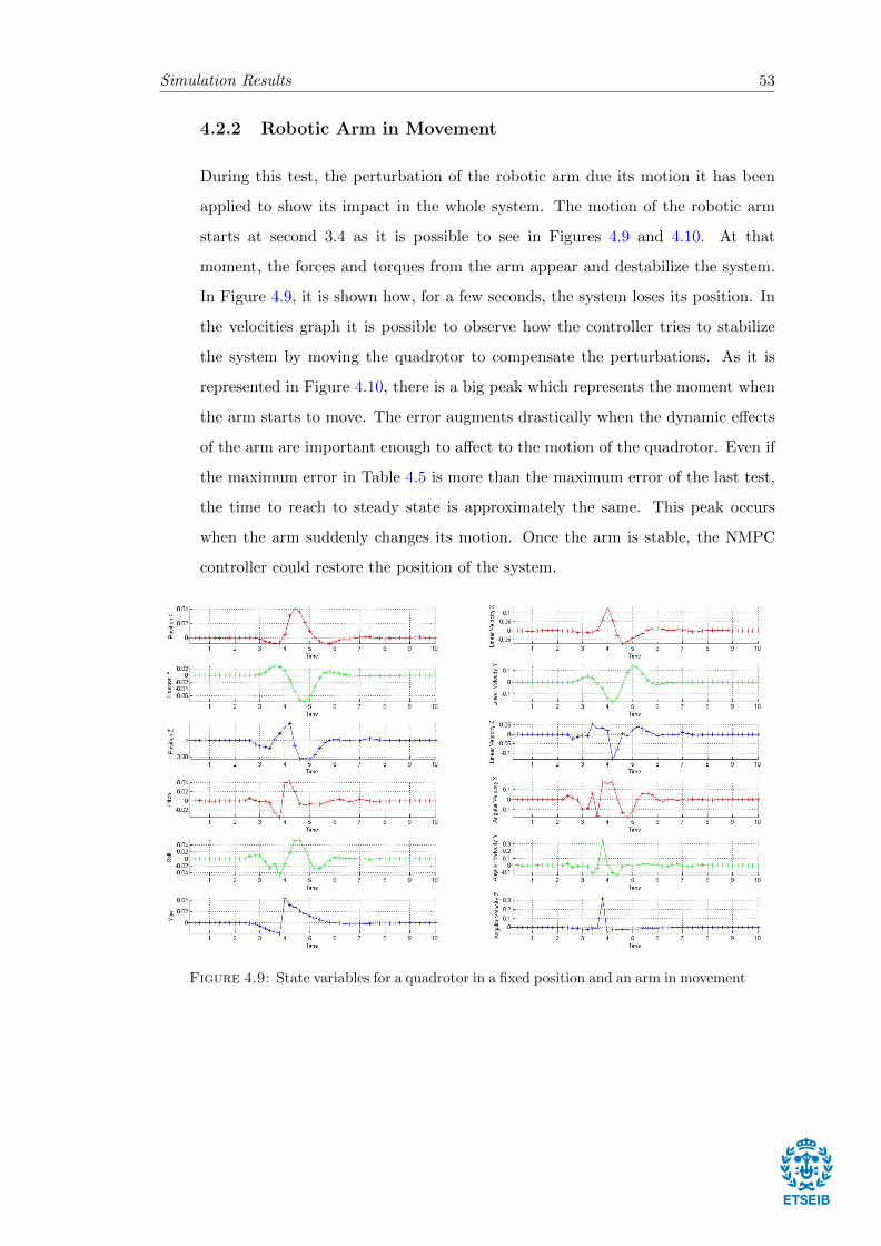
Simulation Results 53
4.2.2 Robotic Arm in Movement
During this test, the perturbation of the robotic arm due its motion it has been
applied to show its impact in the whole system. The motion of the robotic arm
starts at second 3.4 as it is possible to see in Figures 4.9 and 4.10. At that
moment, the forces and torques from the arm appear and destabilize the system.
In Figure 4.9, it is shown how, for a few seconds, the system loses its position. In
the velocities graph it is possible to observe how the controller tries to stabilize
the system by moving the quadrotor to compensate the perturbations. As it is
represented in Figure 4.10, there is a big peak which represents the moment when
the arm starts to move. The error augments drastically when the dynamic effects
of the arm are important enough to affect to the motion of the quadrotor. Even if
the maximum error in Table 4.5 is more than the maximum error of the last test,
the time to reach to steady state is approximately the same. This peak occurs
when the arm suddenly changes its motion. Once the arm is stable, the NMPC
controller could restore the position of the system.
Figure 4.9: State variables for a quadrotor in a fixed position and an arm in movement
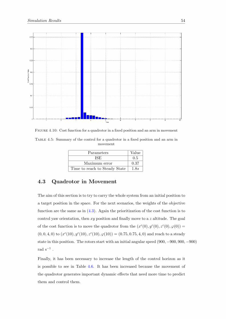
Simulation Results 54
Figure 4.10: Cost function for a quadrotor in a fixed position and an arm in movement
Table 4.5: Summary of the control for a quadrotor in a fixed position and an arm inmovement
Parameters Value
ISE 0.5
Maximum error 0.37
Time to reach to Steady State 1.8s
4.3 Quadrotor in Movement
The aim of this section is to try to carry the whole system from an initial position to
a target position in the space. For the next scenarios, the weights of the objective
function are the same as in (4.3). Again the prioritization of the cost function is to
control yaw orientation, then xy position and finally move to a z altitude. The goal
of the cost function is to move the quadrotor from the (xc(0), yc(0), zc(0), ϕ(0)) =
(0, 0, 4, 0) to (xc(10), yc(10), zc(10), ϕ(10)) = (0.75, 0.75, 4, 0) and reach to a steady
state in this position. The rotors start with an initial angular speed (900,−900, 900,−900)
rad s−1 .
Finally, it has been necessary to increase the length of the control horizon as it
is possible to see in Table 4.6. It has been increased because the movement of
the quadrotor generates important dynamic effects that need more time to predict
them and control them.
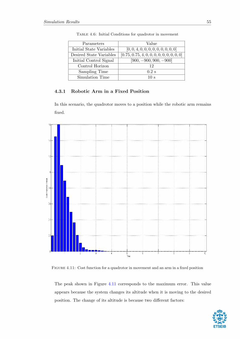
Simulation Results 55
Table 4.6: Initial Conditions for quadrotor in movement
Parameters Value
Initial State Variables [0, 0, 4, 0, 0, 0, 0, 0, 0, 0, 0, 0]
Desired State Variables [0.75, 0.75, 4, 0, 0, 0, 0, 0, 0, 0, 0, 0]
Initial Control Signal [900,−900, 900,−900]
Control Horizon 12
Sampling Time 0.2 s
Simulation Time 10 s
4.3.1 Robotic Arm in a Fixed Position
In this scenario, the quadrotor moves to a position while the robotic arm remains
fixed.
Figure 4.11: Cost function for a quadrotor in movement and an arm in a fixed position
The peak shown in Figure 4.11 corresponds to the maximum error. This value
appears because the system changes its altitude when it is moving to the desired
position. The change of its altitude is because two different factors:
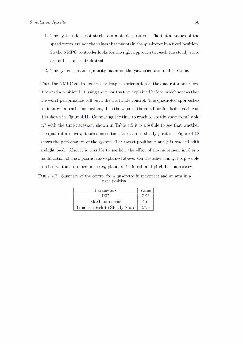
Simulation Results 56
1. The system does not start from a stable position. The initial values of the
speed rotors are not the values that maintain the quadrotor in a fixed position.
So the NMPC controller looks for the right approach to reach the steady state
around the altitude desired.
2. The system has as a priority maintain the yaw orientation all the time.
Then the NMPC controller tries to keep the orientation of the quadrotor and move
it toward a position but using the prioritization explained before, which means that
the worst performance will be in the z altitude control. The quadrotor approaches
to its target at each time instant, then the value of the cost function is decreasing as
it is shown in Figure 4.11. Comparing the time to reach to steady state from Table
4.7 with the time necessary shown in Table 4.5 it is possible to see that whether
the quadrotor moves, it takes more time to reach to steady position. Figure 4.12
shows the performance of the system. The target position x and y is reached with
a slight peak. Also, it is possible to see how the effect of the movement implies a
modification of the z position as explained above. On the other hand, it is possible
to observe that to move in the xy plane, a tilt in roll and pitch it is necessary.
Table 4.7: Summary of the control for a quadrotor in movement and an arm in afixed position
Parameters Value
ISE 7.25
Maximum error 1.6
Time to reach to Steady State 3.75s
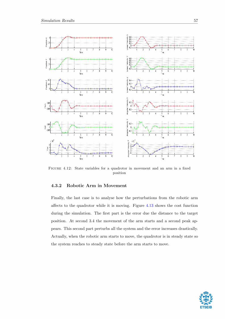
Simulation Results 57
Figure 4.12: State variables for a quadrotor in movement and an arm in a fixedposition
4.3.2 Robotic Arm in Movement
Finally, the last case is to analyse how the perturbations from the robotic arm
affects to the quadrotor while it is moving. Figure 4.13 shows the cost function
during the simulation. The first part is the error due the distance to the target
position. At second 3.4 the movement of the arm starts and a second peak ap-
pears. This second part perturbs all the system and the error increases drastically.
Actually, when the robotic arm starts to move, the quadrotor is in steady state so
the system reaches to steady state before the arm starts to move.
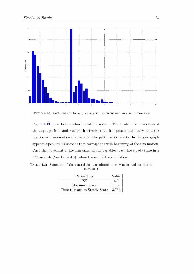
Simulation Results 58
Figure 4.13: Cost function for a quadrotor in movement and an arm in movement
Figure 4.13 presents the behaviour of the system. The quadrotors moves toward
the target position and reaches the steady state. It is possible to observe that the
position and orientation change when the perturbation starts. In the yaw graph
appears a peak at 3.4 seconds that corresponds with beginning of the arm motion.
Once the movement of the arm ends, all the variables reach the steady state in a
3.75 seconds (See Table 4.8) before the end of the simulation.
Table 4.8: Summary of the control for a quadrotor in movement and an arm inmovement
Parameters Value
ISE 6.9
Maximum error 1.19
Time to reach to Steady State 3.75s
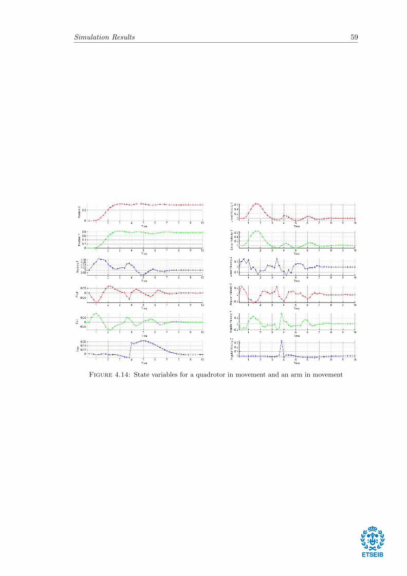
Simulation Results 59
Figure 4.14: State variables for a quadrotor in movement and an arm in movement

Chapter 5
Conclusions and Future Work
5.1 Conclusions
This thesis has proposed an NMPC controller desing to control a quadrotor affected
by a perturbation given by the attachment of a robotic arm and its possible motion.
Also it has been presented a method to couple the dynamics of the UAV and the
robotic arm. Moreover, the algorithm designed and implemented is independent
from the parameterized models used to model both the quadrotor and the arm.
So in this thesis it has been described a general algorithm able to be applied with
any dynamic model. By using the results of the experiments, several conclusions
for this project can be reached:
• First of all, it was possible to make a model of the quadrotor by taking
parameters from different studies. Also, a model of the robotic arm was
made. However, some parameters were modified to increase the perturbation
effect.
• At the light of the results, it can be stated that the NMPC strategy is able to
control a quadrotor with dynamic perturbations. The behaviour in the five
scenarios have been accurate and with an acceptable accuracy. Moreover, it
has checked the relevance of the prediction horizon to reach steady state and
its impact in the CPU performance.
• All these cases are based on a simulation environment because the code is not
optimized enough to test it with real qudrotors. Actually, each simulation
takes between 30-40 minutes to obtain all the results.
61
Conclusions and Future Work 62
• In order to minimize the impact of the perturbation, it is important to design
smooth motions of the arm.
• After all these simulations it is possible to conclude that the most important
parts of the algorithm are the dynamic model of the plant and the prediction
horizon:
– An accurate model allows to predict the behaviour of the system and
then to find the optimal sequence of control inputs. If the model and the
real plant are significantly different, the control signals can not bring the
system to a desired state.
– On the other hand, depending of the maneuver, the horizon has to be
large enough to predict and control the behavior of the system. If the
horizon is not large enough, the system has not time to control its inertia
and reach the desired state values. For a quadrotor in a fixed position,
a large horizon is not necessary because the system is near of its desired
point. But for a quadrotor in movement, in order to reach a specific
position and not surpass it, the horizon has to be enough to have time
to control the reactions.
5.2 Future Work
During the steps of this project, new interesting topics have appeared to be studied
in depth. Some of them are just improvement of the project here presented, and
others are new fields of study to expand the control possibilities of the quadrotor.
In this way, a nice research could be optimize the code to implement it to a real
system. In order to do it, would be important to reduce the computational time
by applying a faster solver of the problem. Also, it would be interesting develop
an algorithm able to calculate the minimum control horizon necessary to find the
steady state. Updating this horizon, the system would always calculate only the
necessary steps to control the quadrotor and a lot of operations would be avoided.
Another important task would be to study the effect of change the dynamic of the
arm by modifying its parameters online. This effect would simulate when the arm
starts to carry some object in its end-effector or if some joints start to fail.

Conclusions and Future Work 63
Also it would be interesting to develop a method to change the application point
of the arm perturbation to a generic point of the quadrotor. In order to achieve it,
it is necessary to study the effects due to apply a force and a torque in a different
point of the CoG of the whole system.
Finally, another important research would be include the state variables of the
joints and the end-effector inside the NMPC. By this technique would be obtained
a more accurate control of the system. Also it would be possible to include a cost
function of the end-effector to accomplish some specific tasks.

Bibliography
Abdel-Malek, K. and Othman, S. (1999). Multiple sweeping using the denavit–
hartenberg representation method. Computer-Aided Design, 31(9):567–583.
Alexis, K., Nikolakopoulos, G., and Tzes, A. (2010). Experimental model predic-
tive attitude tracking control of a quadrotor helicopter subject to wind-gusts.
18th Mediterranean Conf. on Control Automation (MED), page 1461–1466.
Allen, P. K., Timcenko, A., and Yoshimi, B.and Michelman, P. (1993). Auto-
mated tracking and grasping of a moving object with a robotic hand-eye system.
Robotics and Automation, IEEE Transactions, 9:152–165.
Bangura, M. and Mahony, R. (2012). Nonlinear dynamic modeling for high per-
formance control of a quadrotor. Australasian Conference on Robotics and Au-
tomation, pages 1–10.
Belkheiri, M., Rabhi, A. Hajjaji, A. E., and Pegard, C. (2012). Different lin-
earization control techniques for a quadrotor system. In 2nd Int. Conf. on
Communications, Computing and Control Applications (CCCA), pages 1–6.
Benallegue, A., Mokhtari, A., and Fridman, L. (2006). Feedback linearization and
high order sliding mode observer for a quadrotor UAV. Workshop on Variable
Structure Systems, pages 365–372.
Bicchi, A. and Tonietti, G. (2004). Fast and” soft-arm” tactics [robot arm design].
Robotics and Automation Magazine, 11:22–33.
Bouabdallah, S. (2007). Design and control of quadrotors with application to
autonomous flying. Master’s thesis, Ecole Polytechnique federale de Lausanne.
Bouabdallah, S., Murrieri, P., and Siegwart, R. (2004). Design and control of
an indoor micro quadrotor. In Robotics and Automation, 2004. Proceedings.
65
Bibliography 66
ICRA’04. 2004 IEEE International Conference on, volume 5, pages 4393–4398.
IEEE.
Bouffard, P. (2012). On-board Model Predictive Control of a Quadrotor Heli-
copter: Design, Implementation, and Experiments. Master’s thesis, California
University Berkeley Dept. of Computer Sciences.
Bresciani, T. (2008). Modelling, identification and control of a quadrotor heli-
copter. Master’s thesis, Lund University Dept Of Automatic Control.
Corke, P. (2011). Robotics, vision and control: fundamental algorithms in MAT-
LAB. Springer.
Featherstone, R. and Orin, D. (2000). Robot dynamics: Equations and algorithms.
In ICRA, pages 826–834.
Fukuda, T. (1985). Flexibility control of elastic robotic arms. Journal of Robotic
Systems (ISSN 0741-2223), 2:73–88.
Grancharova, A., Grotli, E., and Johansen, T. (2012). Distributed mpc-based path
planning for UAVs under radio communication path loss constraints. Master’s
thesis.
Gruene, L. and Pannek, J. (2011). Nonlinear Model Predictive Control. Theory
and Algorithms. Springer.
Hayati, S. (1986). Hybrid position/force control of multi-arm cooperating robots.
Robotics and Automation. Proceedings. 1986 IEEE International Conference,
3:82–89.
Herrera, R. T., Alcantara, S. M., C., J. A. M., and Velazquez, A. S. (2012).
Serial and Parallel Robot Manipulators - Kinematics, Dynamics, Control and
Optimization, chapter Kinematic and Dynamic Modelling of Serial Robotic Ma-
nipulators Using Dual Number Algebra. InTech.
Hussein, W. M. (2008). Quadrotor design, simulation and implementation. Mas-
ter’s thesis, Arab Academy of Science and Technology.
Johnson, W. (1994). Helicopter Theory. Dover.
Bibliography 67
Khosla, P. K. and Kanade, T. (1987). An algorithm to estimate manipulator
dynamics parameters. Technical report, Institute of Software Research.
Kis, L. and Lantos, B. (2011). Sensor fusion and actuator system of a quadrotor
helicopter. Electrical Engineering, 53(3-4):139–150.
La Civita, M., Papageorgiou, G., Messner, W., and Kanade, T. (2006). Design and
flight testing of an H controller for a robotic helicopter. Journal of Guidance,
Control, and Dynamics, 29:485–494.
Leishman, J. G. (2002). The breguet-richet quad-rotor helicopter of 1907. Verti-
flite, 47:58–60.
Martinez, V. (2007). Modeling of flight dynamics of a quadrotor helicopter. Mas-
ter’s thesis, University School of Engineering, Aerospace Sciences.
Mellinger, D. and V., K. (2011). Minimum snap trajectory generation and control
for quadrotors. Int. Conf. on Robotics and Automation (ICRA), pages 2520–
2525.
Nonami, K. (2006). Prospect and recent research and development for civil use
autonomous unmanned aircraft as UAV and MAV. Journal of system Design
and Dynamics, 1:120–128.
Noth, A., Bouabdallah, S., and Siegwart, R. (2004). PID vs LQ control techniques
applied to an indoor micro quadrotor. International Conf. on Intelligent Robots
and Systems, pages 2451–2456.
Oleg, Y. (2009). Development and testing of the miniature aerial delivery system
snowflake. 20TH AIAA Aerodynamic deceleration systems technology conference
and seminar.
Pounds, P. (2007). Design, construction and control of a large quadrotor micro air
vehicle. Master’s thesis, Australian National Unversity.
Pounds, P., Mahony, R., and Corke, P. (2006). Modelling and control of a quad-
rotor robot. Proceedings Australasian Conference on Robotics and Automation.
Raemaekers, A. (2007). Design of a model predictive controller to control uavs.
Traineeship report, Technische Universiteit Eindhowen, Netherlands.
Bibliography 68
Romero, H., Salazar, S., and Lozano, R. (2009). Real-time stabilization of an
eight-rotor UAV using optical flow. Robotics, IEEE Transactions, 25:809–817.
Sanramaria, A. and Andrade, J. (2014). Hierarchical task control for aerial inspec-
tion. euRathlon-ARCAS Workshop and Summer School on Field Robotics.
Shin, J., Fujiwara, D., Nonami, K., and K., H. (2005). Model-based optimal
attitude and positioning control of small-scale unmanned helicopter. Robotica,
23:51–63.
Sydney, N., Smyth, B., and Paley, D. A. (2013). Dynamic control of autonomous
quadrotor flight in an estimated wind field. In Decision and Control (CDC),
2013 IEEE 52nd Annual Conference on, pages 3609–3616. IEEE.
Velliste, M., Perel, S., Spalding, M. C., Whitford, A. S., and Schwartz, A. B.
(1995). Cortical control of a prosthetic arm for self-feeding. Nature, 453:1098–
1101.
Vries, E. and Subbarao, K. (2010). Backstepping based nested multi-loop con-
trol laws for a quadrotor. Int. Conf. on Control Automation Robotics Vision
(ICARCV), pages 1911–1916.
Wai Weng, K. (2006). Design and control of an indoor micro quadrotor. Research
and Development, 2006. SCOReD 2006, pages 173 – 177.
Zhu, B. and Huo, W. (2010). Trajectory linearization control for a quadrotor
helicopter. IEEE Int. Conf. on Control and Automation (ICCA), pages 34–39.