iv

CONTROLLER PERFORMANCE OF P, PI AND NEURAL NETWORK

CONTROL IN VINYL ACETATE MONOMER PROCESS

FAIZAL NAZARETH IBRAHIM

A thesis submitted in fulfillment of the

requirements for the award of the degree of

Bachelor of Chemical Engineering

Faculty of Chemical & Natural Resources Engineering

University Malaysia Pahang

May, 2008

v

I declare that this thesis entitled “Controller Performance of P, PI and Neural

Network Control in Vinyl Acetate Monomer Process” is the result of my own

research except as cited in the references. The thesis has not been accepted for any

degree and is not concurrently submitted in candidature of any degree.

Signature : ………………………...

Name : Faizal Nazareth Ibrahim

Date : ………………………...

vi

In the Name of Allah, Most Gracious, Most Merciful.

All praise and thanks are due to Allah Almighty and peace and blessings be upon His

Messenger.

To mum and dad, thanks for the love and support.

vii

ACKNOWLEDGEMENT

First of all, I feel grateful to Allah s.w.t for giving me strength and good

health in order to complete this thesis. I also would like to convey my thankful to my

supervisor, Miss Rohaida bte Che Man for her help and guidance for this thesis. Not

forgotten big thanks and grateful to my co-supervisor and also my panel Encik Noor

Asma Fazli Abdul Samad for being my personal navigator who always gives me

courage and his kindness on delivering me his knowledge on writing the thesis. With

only their professional help and guidance make this thesis completely finish.

Besides that, I also would like to dedicate my appreciation to all my lecturers

in the Faculty of Chemical Engineering and Natural Resources (FKKSA) for their

support and motivation during this project development. Their view, advice and

opinion really help and contribute to my understanding for this thesis.

Thanks for all my colleagues that have support me a lot and their assistance

along the development of this thesis. Their kind and tips are useful indeed. And lastly

to my beloved parent and family for being my inner strength all the time.

viii

ABSTRACT

This research is about investigating the controller performance between P, PI

and Neural Network control in Vinyl Acetate Monomer (VAC) Process. The

manufacturing process is about vapor-phase reaction converting ethylene (C2H4),

oxygen (O2) and acetic acid (HAc) into vinyl acetate (VAc) with water (H2O) and

carbon dioxide (CO2) as byproducts. The data from the process are successfully

generated and the simulation of the dynamic response is done with further analysis of

P, PI control and Neural Network control. The study is focusing on the column

section process as the clear view of the control performance is observed. The

Proportional (P) and Proportional Integral (PI) control are type of controller that used

in the process. The Neural Network control then is a control mechanism that has the

similar system of human neurons for processing information data. It consists of

network of neurons that have weight in each network and built generally in layers. As

the analysis result of P and PI control showed that there are some unsatisfying

results, Neural Network Control is then developed to see the changes. In Neural

Network control, the data has been trained and validate to get the better response

before applied again to the process to see the improvement. At the end, Neural

Network has visualized the better control performance as the unsatisfying response of

P and PI control have been improvised.

ix

ABSTRAK

Kajian ini adalah untuk mempelajari perbezaan prestasi antara kawalan PID

dan kawalan Hubungan Neural dalam contoh kes daripada proses penghasilan Vinyl

Acetate. Proses reaksi fasa gas ini menghasilkan Vinyl Acetate (VAC) daripada

ethylene (C2H4), oksigen (O2) dan asid asetik (HAc) dan air (H2O) serta karbon

dioksida (CO2) sebagai produk sampingan. Data daripada proses ini telah ditafsir

keluar dengan baik dan simulasi dinamik respon dilakukan beserta analisis kontrol P

dan PI dan juga kontrol hubungan neural. Kajian ini juga difokuskan pada bahagian

proses pengasingan kolum untuk pemerhatian yang lebih jelas kepada prestasi

kawalan. Kawalan P dan PI adalah kawalan yang digunakan di dalam proses ini.

Kawalan Hubungan Neural pula adalah kawalan yang mirip kepada system

tranformasi maklumat neurons manusia. Ianya mengandungi jaringan neuron dan

berat tersendiri oleh setiap jaringan hubungan itu. Oleh kerana hasil analisis daripada

kawalan P dan PI telah menunjukkan hasil yang kurang memuaskan, kawalan neural

telah diimplimentasikan untuk melihat sebarang perubahan. Pada akhir kajian,

kawalan neural telah menunjukkan bahawa hasil kawalan itu dapat diperbetulkan dan

seterusnya melihatkan keberkesanan kawalan neural berbanding kawalan P dan PI.

x

TABLE OF CONTENT

CHAPTER TITLE PAGE

TITLE PAGE iv

DECLARATION v

DEDICATION vi

ACKNOWLEDGEMENT vii

ABSTRACT viii

ABSTRAK ix

TABLE OF CONTENT x

LIST OF TABLES xii

LIST OF FIGURES xiii

LIST OF SYMBOLS xv

1 INTRODUCTION 1

1.1 Introduction 1

1.2 Problem Statement 2

1.3 Objectives of Study 2

1.4 Scope of study 3

2 LITERATURE REVIEW 4

2.1 The Vinyl Acetate Monomer (VAC) Process 4

2.2 Feedback Control 6

2.3 Block Diagram and Closed-Loop Response 8

2.4 Proportional Integral Derivative (PID) Controller 10

2.41 Effect on Proportional (P) Control 10

2.42 Effect on PI control 13

2.43 Effect on PID control 13

2.5 Artificial Neural Network Control 14

xi

3 METHODOLOGY 17

3.1 Overview 17

3.2 Work Flow 18

3.3 Data Generation 19

3.4 Specifying Column Section 20

3.5 Proportional (P) and Proportional Integral (PI) Control 21

3.6 Neural Network Control 21

4 RESULT AND DISCUSSION 23

4.1 Overview 23

4.2 Result for P control 24

4.3 Result for PI control 25

4.4 Disturbance Present of P control 26

4.5 Disturbance Present of PI control 27

4.6 The Identified Data 28

4.7 Training and Validation 29

4.8 Final Result of Neural Network Control 31

4.9 Comparison and Analysis 32

5 CONCLUSION AND RECOMMENDATION 34

5.1 Conclusion 34

5.2 Recommendation 35

REFERENCES 36

APPENDIX 38-44

xii

LIST OF TABLES

TABLE NO. TITLE PAGE

4.1 Mean square error for validation and training of Vapor In (Vap-In) 29 4.2 Mean square error for validation and training Org. Level (Org-L) 31

xiii

LIST OF FIGURES

FIGURE NO. TITLE PAGE 2.1 Vinyl acetate monomer process flowsheet 5 2.2 General process block diagram 6 2.3 Corresponding feedback loop 7 2.4 The general closed loop system 8 2.5 Closed loop response of setpoint changes 12 2.6 Closed loop response of disturbance change 12 2.7 Effect of gain on the closed-loop response with PID control 14 2.8 Single processing node 15 2.9 Neural Network Layer 15 3.1 Work flow diagram 18 3.2 Data Generation 19 3.3 Column section 20 3.4 Neural Network implementation and training 22 4.1 Result for P controller 24 4.2 Result for PI controller 25 4.3 Result for P controller with disturbance 26 4.4 Results for PI controller with disturbance 27 4.5 Vapor-In Response of P and PI control 28 4.6 Organic Level Response of P and PI control 28

xiv

4.7 Training and Validation for Vapor In (Vap-In) 29 4.8 Training and Validation for Organic Level (Org-L) 30 4.9 Final Result of Neural Network Control for Vapor In (Vap-In) 32 4.10 Final Result of Neural Network Control for Organic Level (Org-L) 32 4.11 Result of P and PI control for Vapor In (Vap-In) 32 4.12 Final Result of Neural Network Control for Vapor In (Vap-In) 32 4.13 Result of P and PI control for Organic Level (Org-L) 33 4.14 Final Result of Neural Network Control for Organic Level (Org-L) 33

xv

LIST OF SYMBOLS

SYMBOLS / TITLE ABBREVIATION

m Manipulated variable

d Potential disturbance

y Output

my Measured value

spy Set point value ∈ Deviation error

pG Process

dG Disturbance

mG Measurement

cG Controller

fG Final Control Element

cK Gain pK ' & dK ' Closed-loop static gains τ Time constant dt Dead time

CHAPTER 1

INTRODUCTION

1.1 Introduction In 1998, an additional model of a large, industrially relevant system, a vinyl

acetate monomer (VAC) manufacturing process, was published by Luyben and

Tyreus. The VAC process contains several standard unit operations that are common

to many chemical plants. Both gas and liquid recycle streams are present as well as

process-to-process heat integration. Luyben and Tyreus presented a plantwide control

test problem based on the VAC process. The VAC process was modeled in TMODS,

which is a proprietary DuPont in-house simulation environment, and thus, it is not

available for public use (Luyben and Tyrus, 1998).

The model of the VAC process is developed in MATLAB, and both the

steady state and dynamic behavior of the MATLAB model are designed to be close

to the TMODS model. Since the MATLAB model does not depend on commercial

simulation software and the source code is open to public, the model can be modified

for use in a wide variety of process control research areas. For each unit, design

assumptions, physical data, and modeling formulations are discussed. There are some

differences between the TMODS model and the MATLAB model, and these

differences together with the reasons for them are pointed out. Steady state values of

the manipulated variables and major measurements in the base operation are given.

Production objectives, process constraints, and process variability are summarized

based on the earlier publication. All of the physical property, kinetic data, and

process flowsheet information in the MATLAB model come from sources in the

open literature.

2

The manufacturing process is about vapor-phase reaction converting ethylene

(C2H4), oxygen (O2) and acetic acid (HAc) into vinyl acetate (VAc) with water (H2O)

and carbon dioxide (CO2) as byproducts. It has both gas and liquid recycle streams

with real components. The process contain 10 basic unit operations that include a

catalytic plug flow reactor, a feed-effluent heat exchanger (FEHE), a separator, a

vaporizer, a gas compressor, an absorber, a carbon dioxide (CO2) removal system, a

gas removal system, a tank for the liquid recycle stream and an azeotropic distillation

column with a decanter plants (Luyben and Tyrus, 1997). This process is focusing

the data response of the column section to give the clear view of the controller

performance. The control response of P, PI and Neural Network controller is

observed for further analysis.

1.2 Problem Statement Generally, the actual data of Vinyl Acetate Monomer (VAC) process is

controlled by either P or PI control. The suitability using Neural Network Control

alongside the actual P and PI control and the capability of the controller to improve

the unsatisfied result is investigated and analyzed.

1.3 Objectives of Study The aims of this study are:

To generate data the of control process in Vinyl Acetate Monomer (VAC)

besides investigating the controller performance of PI and P control compared to

Neural Network controllers in Vinyl Acetate Monomer (VAC) process.

3

1.4 Scope of Study

In order to achieve the objectives, the study is specified into those scopes:

a) To generate data from Vinyl Acetate (VAC) monomer process

b) To simulate dynamic response of the data.

c) To analyze the performance of the controller response of P, PI control and

Neural Network control.

d) To analyze and compare the performance of the controllers.

CHAPTER 2

LITERATURE REVIEW 2.1 The Vinyl Acetate Monomer (VAC) Process

The vinyl acetate monomer (VAC) manufacturing process consist 10 basic

unit operation which include catalytic plug flow reactor, a feed-effluent heat

exchanger (FEHE), a separator, a vaporizer, a gas compressor, an absorber, a carbon

dioxide (CO2) removal system, a gas removal system, a tank for the liquid recycle

stream and an azeotropic distillation column with a decanter plants (Luyben and

Tyrus, 1997). The manufacturing process is about vapor-phase reaction converting

ethylene (C2H4), oxygen (O2) and acetic acid (HAc) into vinyl acetate (VAc) with

water (H2O) and carbon dioxide (CO2) as byproducts. An inert, ethane (C2H6), enters

with the fresh ethylene feed stream. The reactions are as below:

021

2322342 HCHOCOCHCHOCOOHCHHC +=→++ (2.1)

OHCOOHC 22242 223 +→+ (2.2)

The exothermic reactions occur in a reactor containing tubed packed with

precious metal catalyst on a silica support. Heat is removed from the reactor by

generating steam on the shell side of the tubes. Water flows to the reactor from a

steam drum, to which make-up water (BFW) is provided. The steam leaves the drum

as saturated vapor. The reactions are irreversible and the reaction rates have an

Arrhenius-type dependence on temperature.

5

Figure 2.1 shows the process flow sheet with location of the manipulated

variables. The numbers on the streams are the same as those given by Luyben and

Tyreus (1997).

Figure 2.1: Vinyl acetate monomer process flowsheet

The reactor effluent leaves through a process-to-process heat exchanger,

where the cold stream is the gas recycle. Then, the effluent is cooled with cooling

water and the vapor (oxygen, ethylene, carbon dioxide and ethane) and liquid (vinyl

acetate, water and acetic acid) are separated. The vapor stream from the separator

goes to the compressor and the liquid stream from the separator becomes a part of the

feed to the azeotropic distillation column. The gas from the compressor enters the

bottom of an absorber, where the remaining vinyl acetate is recovered. A liquid

stream from the base is recirculated by a cooler and fed to the middle of the absorber.

To provide scrubbing, the liquid acetic acid that hes been cooled is fed into the top of

the absorber. The liquid bottoms product from the absorber combines with the liquid

from the separator as the feed stream to the distillation column (Luyben and Tyrus,

1997).

Some of the overhead gas exiting the absorber enters the carbon dioxide

removal system is simplified by treating it as component separator with a certain

6

efficiency that is a function of rate and composition. The gas stream minus carbon

dioxide is split, with part going to the purge for removal of the inert ethane and the

rest combines with large recycle gas stream goes to the feed-effluent heat exchanger

also with added fresh ethylene feed stream. Steam is used to vaporize the liquid in

the vaporizer where the gas recycle stream, the fresh acetic acid feed and the recycle

liquid acetic acid enters. The gas stream from the vaporizer is further heated to the

desired reactor inlet temperature in a trim heater using steam. To keep the oxygen

composition in the recycle loop outside the explosives region, fresh oxygen is added

to the gas stream from the vaporizer.

The azeotropic distillation column then separates the vinyl acetate and water

from the unconverted acetic acid. The overhead product is condensed with cooling

water and the liquid goes to the decanter, where the vinyl acetate and water phase

separate. The bottom product from the distillation column contains acetic acid, which

recycles back to the vaporizer along with fresh make-up acetic acid. Part of this

bottom product is the wash acid used in the absorber after being cooled (Mc Avoy,

1998).

2.2 Feedback Control

In general process, feedback control process has an output y , a potential

disturbance d, and an available manipulated variable m. (George Stephanopoulus,

2004). The process is shown in Figure 2.2 below:

Figure 2.2: General process block diagram

The disturbances, d or load change is an unpredictable manner and the aim of

the control process is to keep the value of the output, y at the desired levels. A

feedback control action takes the following steps. First, the value of the output (flow,

7

pressure, liquid level, temperature, composition) will be determined using the

appropriate measuring device with my be the value indicated by the measuring

sensor. Then, the indicated value my is compared to the desired value spy (set point)

of the output and the deviation (error) would be msp yy −∈= . The value of the

deviation ∈ is supplied to the main controller. The controller in turn changes the

value of the manipulated variable m in such way as to reduce the magnitude of the

deviation∈. Usually the controller does not affect the manipulated variable directly

but through another device (usually a control valve), known as the final control

element.

Figure 2.3 shows the notified steps. The system in Figure 2.2 is known as

open loop, in contrast to the feedback controlled system in Figure 2.3 which is called

closed loop. When value of d or m change, the response of the first step is

categorized open loop response while the second step is the closed loop response.

controller mechanism d

Ysp + e c m y

-

ym

Figure 2.3: Corresponding feedback loop

2.3 Block Diagram and the Closed-Loop Response

For the generalized closed-loop system showed in Figure 2.4, it has four

components (process, measuring device, controller mechanism and final control

element) which corresponding transfer functions relating its output to the inputs can

be written.

Controller Process Final

control element

Measuring device

8

Process

Ysp e(s) c(s) m(s) + + y(s) + - Controller Final control element ym(s) Measuring device

Figure 2.4: The generalized close-loop system

In particular, if the dynamics of the transmission lines, are neglect: Process:

)()()()()( sdsGsmsGsy dp += (2.3)

Measuring device:

)()()( sysGsy mm = (2.4)

Controller mechanism:

)()()( sysys mSP −=∈ comparator (2.5)

)()()( ssGsc c ∈= control action (2.6)

Final Control Element :

)()()( scsGfsm = (2.7)

where fcmdp GandGGGG ,,, are the transfer function between the corresponding

inputs and outputs (McMillan, 1994). The series of blocks between the comparator

and the controlled output (i.e., cG , fG and pG ) constitutes the forward path, while

Gc(s) Gf(s)

Gm(s)

Gd(s)

Gp(s)

9

the block mG is on the feedback path between the controlled output and the

comparator.

Algebraic manipulation of the equations above yields

)]()()()[()()( sysGsysGsGsm mSPcf −= (2.8)

completing back the equation (2.3) give:

)()()]}()()()[()(){()( sdsGsysGsysGcsGfsGpsy dmSP +−= (2.9)

and after readjusting

)()()()()(1

)()()()()()(1

)()()()( sdsGmsGcsGfsGp

sGdsysGmsGcsGfsGp

sGcsGfsGpsy SP+

++

=

(2.10)

This equation gives the closed-loop response of the process. It is composed of two

terms. The first term shows the effect on the output of change in the set point, while

the second term tells the effect on the output of a change in the load (disturbance).

The corresponding transfer functions are known as closed-loop transfer functions. In

particular,

SPm

p GGGG

=+1

(2.11)

is the closed loop transfer function for a change in the set point and

loadm

d GGGG

=+1

(2.12)

is the closed loop transfer function for a change in the load.

10

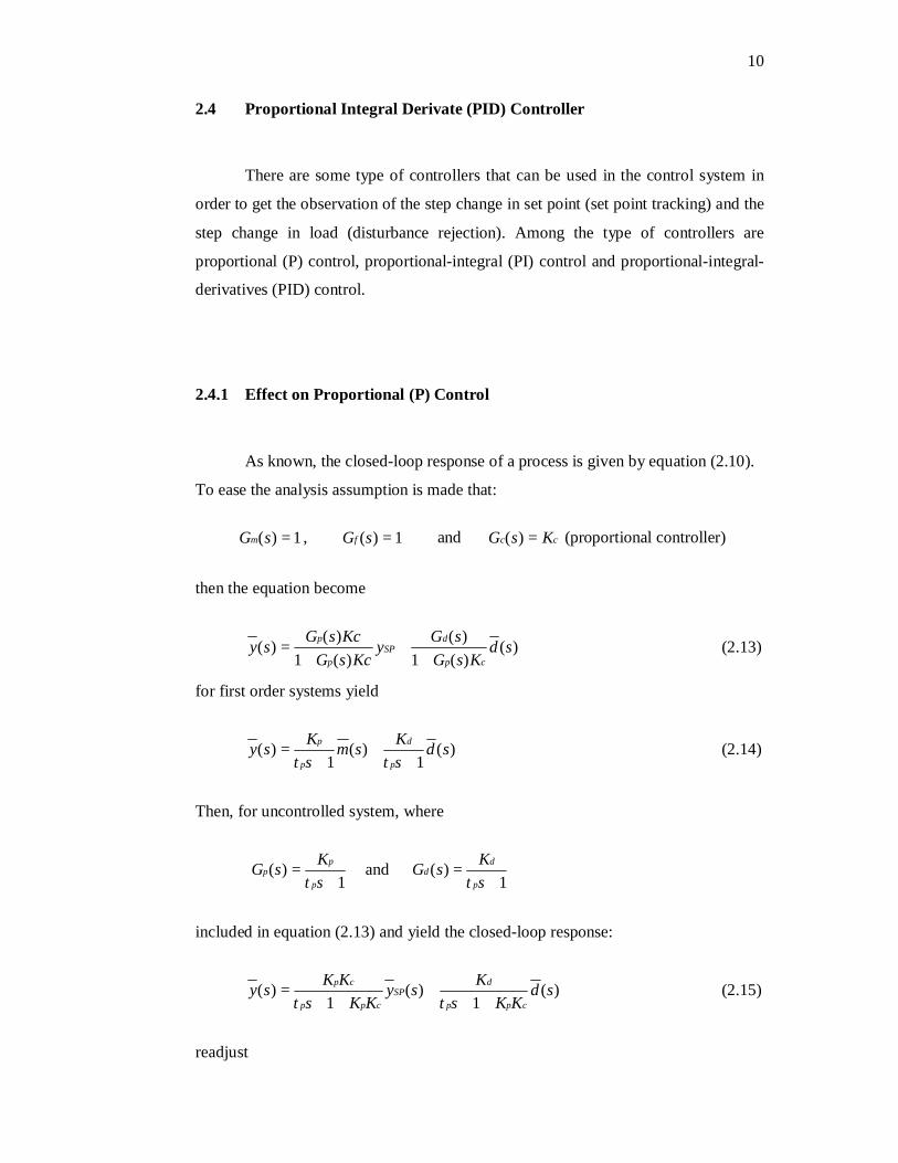
2.4 Proportional Integral Derivate (PID) Controller

There are some type of controllers that can be used in the control system in

order to get the observation of the step change in set point (set point tracking) and the

step change in load (disturbance rejection). Among the type of controllers are

proportional (P) control, proportional-integral (PI) control and proportional-integral-

derivatives (PID) control.

2.4.1 Effect on Proportional (P) Control

As known, the closed-loop response of a process is given by equation (2.10).

To ease the analysis assumption is made that:

1)( =sGm , 1)( =sGf and cc KsG =)( (proportional controller)

then the equation become

)()(1)(

)(1)()( sd

KsGsGy

KcsGKcsGsy

cp

dSP

p

p

++

+= (2.13)

for first order systems yield

)(1

)(1

)( sdsKsm

sKsy

p

d

p

p

++

+=

ττ (2.14)

Then, for uncontrolled system, where

1

)(+

=sKsG

p

pp

τ and

1)(

+=

sKsG

p

dd

τ

included in equation (2.13) and yield the closed-loop response:

)(1

)(1

)( sdKKs

KsyKKs

KKsycpp

dSP

cpp

cp

+++

++=

ττ (2.15)

readjust

11

)(1'

')(1'

')( sds

Ksys

Ksyp

dSP

p

p

++

+=

ττ (2.16)

where

cp

pp

KK+=

1' τ

τ , cp

cpp

KKKKK

+=

1' and

cp

dd

KKKK

+=

1'

K’p and K’d also known closed-loop static gains.

As the result the closed-loop response of a first order system is still is the first

order system with respect to load and set point changes. The closed-loop response

has become faster than the open-loop response to the change in set point or load, due

to the time constant that has been reduced and also the static gains that have been

decreased.

In order to get better observation to the effect of this proportional controller,

the resulting closed-loop responses is reviewed and examined with set point and the

disturbance changes.

For change in the set point where s

ysp1

= and 0)( =sd , which insert to equation

(2.16) resulting

ss

Ksyp

p 11'

)(+

=τ

in the inverse mode give

)1(')( '/ ptepKty τ−−= (2.17)

Figure 2.5 view the response of the closed loop response to set point change.

The ultimate response, after t → ∞, never reaches the desired new set point. There is

a discrepancy called offset which is equal to

offset = (new set point) – (ultimate value of the response)

pK '1−=

cp KK+

=1

1

The offset is the effect of proportional control. It decreases as Kc becomes larger and

generally

12

offset → 0 when Kc → ∞

For change in the disturbance, 0)( =sy sp and s

sd 1)( = . Hence the equation (2.17)

become

ss

Ksy

p

d 11'

')(

+=

τ

inverse give

)1(')( '/ pt

d eKty τ−−= (2.18)

Response in the disturbance change is shown in Figure 2.6. Again the proportional

controller cannot keep the response at the desired set point but it exhibits an offset:

offset = (set point) – (ultimate value of response)

dK '0 −=

cp

d

KKK

+−=

1

The advantage of the proportional control in the presence of disturbance changes, the

response is much closer to the desired set point than not have control at all (Lee,

1998). This effect can be viewed from the Figure 2.6. If the gain Kc is increased the

offset decreases and theoretically

offset → 0 when Kc → ∞

Figure 2.5: Closed-loop response of Figure 2.6: Closed-loop response of

set point change disturbance change