Table of Contents

Executive Summary . . . . . . . . . . . . . . . . . . . . . . . . . . . . . . . . . . . . . . . . . . . . . . . . . . . . 2 pages

Chapters

I. Introduction . . . . . . . . . . . . . . . . . . . . . . . . . . . . . . . . . . . . . . . . . . . . . . . . . . . . . . . . 1

II. Current Disclosure Limitation Techniques . . . . . . . . . . . . . . . . . . . . . . . . . . . . . . . . . . 2

III. The General Data Swapping Disclosure Limitation Technique . . . . . . . . . . . . . . . . . . 2

IV. Advantages of a Data Swap . . . . . . . . . . . . . . . . . . . . . . . . . . . . . . . . . . . . . . . . . . . . . 4

V. Disadvantages of a Data Swap . . . . . . . . . . . . . . . . . . . . . . . . . . . . . . . . . . . . . . . . . . . 4

VI. The Dalenius and Reiss Data Swap . . . . . . . . . . . . . . . . . . . . . . . . . . . . . . . . . . . . . . . 5

VII. A Rank-Based Proximity Swapping Algorithm . . . . . . . . . . . . . . . . . . . . . . . . . . . . . . 6

VIII. Enhancing the Rank-Based Proximity Swap Algorithm . . . . . . . . . . . . . . . . . . . . . . . . 7

IX. Testing the Enhanced Data Swap Theory, The Test Deck . . . . . . . . . . . . . . . . . . . . . . 10

Table 1. Statistics for the Fields Subjected to Swapping . . . . . . . . . . . . . . . . . . . 10

X. Objectives of the Rank-Based Proximity Swap . . . . . . . . . . . . . . . . . . . . . . . . . . . . . . 11

XI. Results of the Testing . . . . . . . . . . . . . . . . . . . . . . . . . . . . . . . . . . . . . . . . . . . . . . . . . 11

Table 2. Comparison of the Observed with the Expected Correlation Coefficients Fora Data Swap with Factor, R = 0.975 . . . . . . . . . . . . . . . . . . . . . . . . . . 120

Table 3. Observed versus Expected Correlation Coefficients of Highly CorrelatedCombinations of Continuous Variables For Various Target Values of R . . . . . . . . . . . . . . . . . . . . . . . . . . . . . . . . . . . . . . . . . . . . . . . . . . . 130

Table 4. Results of the Rank-Based Proximity Swap Test . . . . . . . . . . . . . . . . . 15

Table 5. Optimal Matching/Non-Matching Weights for the EM Procedure for theRank-Based Proximity Swap Versions of the 1993 AHS Microdata File 21

Table 6. Ability of an Intruder to Re-identify Microdata Masked by a Rank-BasedProximity Swapping Routine . . . . . . . . . . . . . . . . . . . . . . . . . . . . . . . . 22

Table 7. Ability of an Intruder to Re-identify Microdata Masked by Kim's RandomNoise Procedure . . . . . . . . . . . . . . . . . . . . . . . . . . . . . . . . . . . . . . . . . . 24

XII. Future Research Topics . . . . . . . . . . . . . . . . . . . . . . . . . . . . . . . . . . . . . . . . . . . . . . . . 24

XIII. Conclusions . . . . . . . . . . . . . . . . . . . . . . . . . . . . . . . . . . . . . . . . . . . . . . . . . . . . . . . . . 25

XIV. References . . . . . . . . . . . . . . . . . . . . . . . . . . . . . . . . . . . . . . . . . . . . . . . . . . . . . . . . . . 26

Appendices

A. Bias Introduced on the Correlation Coefficient by Independent Ordinal Swaps . . 4 pages

B. Construction of a Swapping Interval for a Given Target Coefficient Between the Swapped and Unswapped Values . . . . . . . . . . . . . . . . . . . . . . . . . . . 4 pages

C. Determination of an Appropriate Fixed Interval Length to Give a "K" Percent Average Absolute Difference . . . . . . . . . . . . . . . . . . . . . . . . . . . . . . 2 pages

Executive Summary

For years, the U.S. Bureau of the Census has collected and disseminated data. It has come torealize the importance of these data products for research, analysis, planning, and policy-making. Technological advances of the 1980s have greatly increased the demand for data, particularly forthe microdata products. Users now demand more detailed microdata sets than ever before. Unfortunately, the more information which the Census Bureau provides, the greater the risk thata user can determine the responses for some respondents.

Title 13 requires that the Census Bureau take the necessary steps to ensure the confidentiality ofall respondents. Traditional approaches to disclosure limitation (i.e., supplying the user withmicrodata for only a small sample of the population, using bottom- and top-codes for continuousvariables, and limiting detail-- e.g., use of ranges for some sensitive variables, providinggeographical codes for only highly-populated regions) no longer provide adequate protection forsome of the more sophisticated demands. As a result, the Census Bureau is constantly exploringthe use and development of different disclosure limitation techniques. This paper explores thepossible use of a data-swapping technique.

Data-swapping was first introduced in the late 1970s. In the early 1980s, Dalenius and Reissproved that, when used properly, the technique provided adequate protection to a microdata filewithout altering marginal frequency counts. This procedure has other desirable properties,namely: (1) it removes the relationship between the record and the respondent; (2) it can be usedon sensitive variables, without disturbing the non-sensitive ones; (3) it can be designed toprovide protection where it is most needed; and (4) it is simple to implement.

Data-swapping also has its drawbacks. We see two major disadvantages. First, arbitraryswapping can severely distort the statistics of sub-domains of the universe. This will render thefile inappropriate for research and inference. Second, the implementation of more involvedswapping procedures may require a substantial amount of computer time and storage.

Rank-based proximity swapping (Section VII) appears to retain all the positive attributes (i.e.,easy to implement, adequate masking, etc.), while retaining a sufficient amount of the file’sanalytic validity. The method can be designed to preserve (1) a sufficient proportion of themultivariate dependence/independence relationships, or (2) the means (within prescribedconfidence intervals) of randomly selected subsets.

In Section VIII, we note that rank-based proximity swapping can be designed to providesufficient control of the distortion. Let a and b be two arbitrary continuous fields, which wesubject to swapping. We desire to satisfy one of the two following constraints.

(1) Let R(a, b) and R(a’, b’) be the correlation between the fields before and after theswap. Suppose we desire the swap to reduce the correlation by no more than a factor ofR , 0 < R < 1. That is, E ( R(a’, b’) ) = R * R(a, b). Suppose N(a) is the number of0 0 0

observations between the bottom- and top-coded values for field a. Assume we let P(a)be the maximum percentage of the difference of the ranks ( i.e., the i-th ranked value of acan be swapped with the j-th ranked value if and only if | i - j | < P(a) * N(a) ). Then

P(a)'100(2(Var(a)((1&R0)

(atopc&abotc).

P(a)'100(83(

K0(a

(atopc&abotc).

CPU for ai(sec.)' N(ai)((P(ai)

4%

13000

);

CPU for Total Swap(sec.)'jk

i'1N(ai)((

P(ai)

4%

13000

).

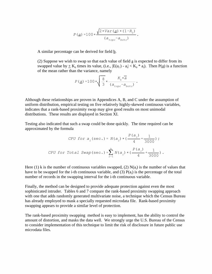
A similar percentage can be derived for field b.

(2) Suppose we wish to swap so that each value of field a is expected to differ from itsswapped value by + K times its value, (i.e., |E(a ) - a | < K * a ). Then P(a) is a function0 i’ i 0 i

of the mean rather than the variance, namely

Although these relationships are proven in Appendices A, B, and C under the assumption ofuniform distribution, empirical testing on five relatively highly-skewed continuous variables,indicates that a rank-based proximity swap may give good results on most unimodaldistributions. These results are displayed in Section XI.

Testing also indicated that such a swap could be done quickly. The time required can beapproximated by the formula

Here (1) k is the number of continuous variables swapped, (2) N(a ) is the number of values thati

have to be swapped for the i-th continuous variable, and (3) P(a ) is the percentage of the totali

number of records in the swapping interval for the i-th continuous variable.

Finally, the method can be designed to provide adequate protection against even the mostsophisticated intruder. Tables 6 and 7 compare the rank-based proximity swapping approachwith one that adds randomly generated multivariate noise, a technique which the Census Bureauhas already employed to mask a specially requested microdata file. Rank-based proximityswapping appears to provide a similar level of protection.

The rank-based proximity swapping method is easy to implement, has the ability to control theamount of distortion, and masks the data well. We strongly urge the U.S. Bureau of the Censusto consider implementation of this technique to limit the risk of disclosure in future public usemicrodata files.

1

CONTROLLED DATA-SWAPPING TECHNIQUES FOR MASKING PUBLIC USE MICRODATA SETS

Richard A. Moore, Jr.Statistical Research Division

US Bureau of the CensusWashington, DC 20233

Abstract

For many years, the U.S. Bureau of the Census has collected and disseminated data. The Bureauhas come to realize the importance of such data for research, analysis, planning, and policy-making. In 1963, the Bureau released a one-in-a-thousand sample file for the 1960 DecennialCensus. Today, microdata files are an important part of our decennial census and demographicsurveys program. The advent of the technological revolution in the early 1980s and theaccessibility of personal computers to small businesses and individuals has greatly increased thedemand for such data. Users now demand large and extremely detailed data sets. Unfortunately,the more information which the Census Bureau provides, the greater the risk that a user candetermine the responses for some respondent.

Title 13 requires that the Census Bureau take the necessary steps to ensure the confidentiality ofall respondents. Since today's data users are more sophisticated than those of the past, it isbecoming difficult to provide the anonymity which the law requires. As a result, the Bureau isnot always able to completely fulfill all requests. This paper gives a brief overview of theevolution of data-swapping techniques and presents a more sophisticated technique than found inthe existing literature.

I. Introduction

For many years, the U.S. Bureau of the Census has recognized its obligation to collect andsupply the nation's data user community with meaningful products. Some of these productsinclude public use microdata sample files. Access to such files allow researchers to conductimportant studies quickly, inexpensively, and efficiently. Without them, all specially requestedtabulations would have to be conducted through a contract with the Census Bureau. This wouldput a tremendous strain on the programming and computer support staffs, since much of theirtime is committed to the day-to-day operations of producing the standard products.

On the other hand, the Census Bureau not only has an obligation to its data users but also to itsdata suppliers. Title 13 requires that it disseminate no product from which specific informationabout any particular respondent can be derived. In the case of a microdata file, this implies thatdata users are not able to query the file for the purpose of identifying individuals. To reduce therisk of respondent identification, it must subject each file to the appropriate disclosure limitationtechniques. Many of these techniques have been in use since 1963, when the Census Bureaureleased its first public use microdata set.

2

II. Current Disclosure Limitation Techniques

The Census Bureau currently uses several standard techniques to mask microdata sets. The firstis a release of data for only a sample of the population. Intruders (i.e., those who query the filefor the sole purpose of identifying particular individuals with unique traits) realize that there isonly a small probability that the file actually contains the records for which they are looking. The Bureau currently releases three public use samples of the decennial census respondents. One is a 1 percent sample of the entire population, the second a 5 percent sample, and the third asample of elderly residents. Each is a systematic sample chosen with a random start. None ofthese files Aoverlap,@ so there is no danger of matching to each other. Most demographic surveysare 1-in-1000 and 1-in-1500 "random" samples. Generally the public use file for each surveycontains records for each respondent.

The second technique involves the limitation of detail. The Census Bureau releases nogeographic identifiers which would restrict the record to a sub-population of less than 100,000. It also Arecodes@ some continuous values into intervals and combines sparse categories. Intruders must have extremely fine detail for other highly sensitive fields in order to positivelyidentify targets.

The third technique protects the detail in sensitive responses in continuous fields. It is referredto as top/bottom-coding. This method collapses extreme values of each sensitive field into asingle value. For example, the record of an individual with an extremely high income would notcontain his exact income but rather a code showing that the income was over $100,000. Similarly the low-income records would contain a code signifying the income was less than $0. In this example $0 is a bottom-code and $100,000 a top-code for the sensitive or high visibilityfield of income.

III. The General Data Swapping Disclosure Limitation Technique

The accessibility of personal computers and the accompanying technology (modems andelectronic data transfer) have allowed data users to handle larger and more detailed data sets thanever before. They also allow the user to compare individual records from Census Bureau-released records with those from other files available to the general public (e.g., real estatedatabases, information released by local governments, etc.). Today's users are demanding largerand more detailed microdata files than ever before. Users are also demanding larger samples,finer geographic detail and relaxation of the top- and bottom-codes. Disclosure limitationtechniques of the 1960s may no longer sufficiently mask the anonymity of the respondents. When used in conjunction with the techniques listed above, data swapping may be a feasibleprocedure to adequately mask data files while providing users with more information.

One of the first references to data swapping is found in Reiss (1980). In his article, the authordescribes interchanging values of individual records within a highly visible field. The swapprotects the univariate distribution of that variable. Since its value belongs to some otherrespondent, each respondent's anonymity is protected. Consider the example below, where

3

income is to be the sensitive field protected.

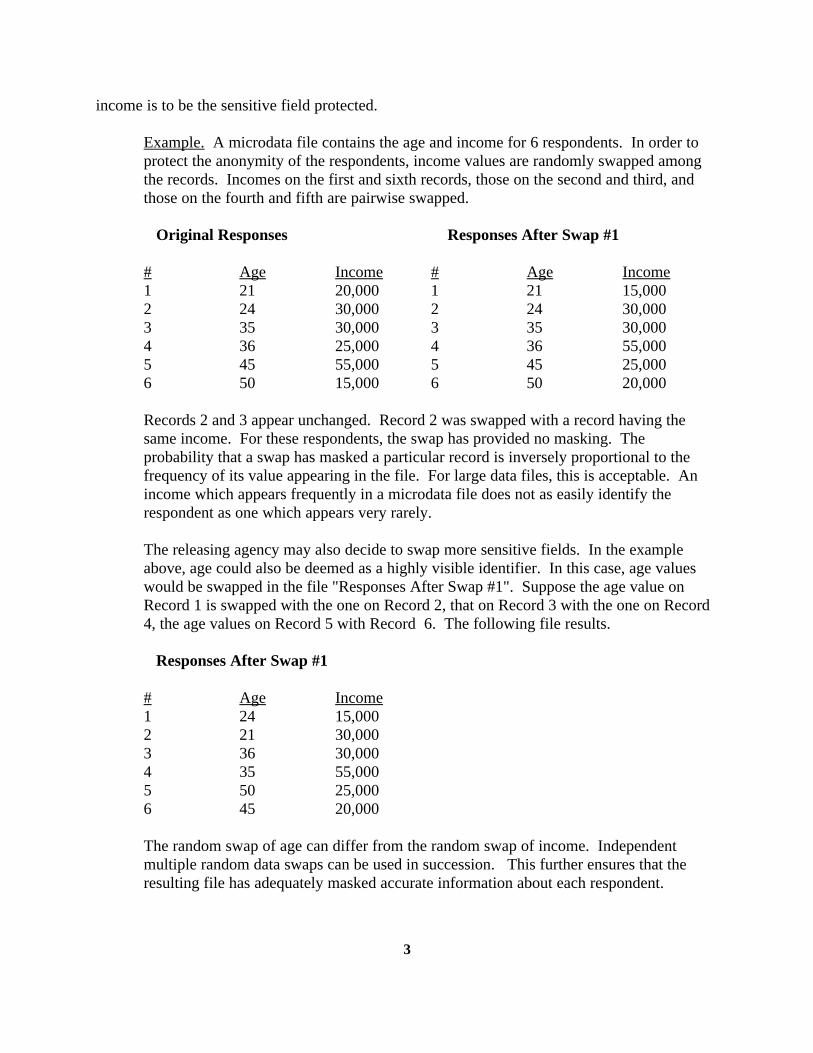
Example. A microdata file contains the age and income for 6 respondents. In order toprotect the anonymity of the respondents, income values are randomly swapped amongthe records. Incomes on the first and sixth records, those on the second and third, andthose on the fourth and fifth are pairwise swapped.

Original Responses Responses After Swap #1

# Age Income # Age Income1 21 20,000 1 21 15,0002 24 30,000 2 24 30,0003 35 30,000 3 35 30,0004 36 25,000 4 36 55,0005 45 55,000 5 45 25,0006 50 15,000 6 50 20,000

Records 2 and 3 appear unchanged. Record 2 was swapped with a record having thesame income. For these respondents, the swap has provided no masking. Theprobability that a swap has masked a particular record is inversely proportional to thefrequency of its value appearing in the file. For large data files, this is acceptable. Anincome which appears frequently in a microdata file does not as easily identify therespondent as one which appears very rarely.

The releasing agency may also decide to swap more sensitive fields. In the exampleabove, age could also be deemed as a highly visible identifier. In this case, age valueswould be swapped in the file "Responses After Swap #1". Suppose the age value onRecord 1 is swapped with the one on Record 2, that on Record 3 with the one on Record4, the age values on Record 5 with Record 6. The following file results.

Responses After Swap #1

# Age Income1 24 15,0002 21 30,0003 36 30,0004 35 55,0005 50 25,0006 45 20,000

The random swap of age can differ from the random swap of income. Independentmultiple random data swaps can be used in succession. This further ensures that theresulting file has adequately masked accurate information about each respondent.

4

IV. Advantages of a Data Swap Any data swapping procedure has the following benefits and advantages.

1. Data swapping masks accurate information about each respondent.

2. If performed on all potential key variables (i.e., variables whose values when takentogether may contribute to the linking of a record with a respondent), swapping removesany relationship between the record and its respondent.

3. This procedure is extremely simple and requires nothing more than a microdata fileand a random number generating routine to implement. The programming is verystraight-forward.

4. The swapping procedure can be used on a select set of one (or more) variables,without disturbing the responses for non-sensitive and non-identifying fields.

5. Swapping of continuous variables provides protection when it is most necessary. Rare and unique responses are generally used to identify respondents. These values arevery likely to be changed. Frequently recurring responses are less likely to be of value toan intruder and less likely to be altered by the swap. (See the income example in SectionIII.)

6. The procedure is not limited to continuous variables, categorical variables (such asrace, sex, occupation) can also be swapped. Care must be used when swappingcategorical variables; otherwise one can greatly decreases the usefulness of the file bylosing the true information and creating a large number of strange combinations (such as male secretaries).

V. Disadvantages of a Data Swap

The advantages of a data swap are listed above, but any data swapping procedure has severaldisadvantages.

1. One disadvantage was briefly mentioned in item 6. Arbitrary categorical swaps canproduce a large number of records with unusual combinations. Arbitrary swaps oncontinuous variables may do the same. For example, a clerk's income may be swappedwith that of a brain surgeon.

2. Another is a function of the number of records in the file and the number of variablesthat are to be subjected to a swap. It may take a significant amount of time and computerresources to swap and store the original file and the swapped version.

5

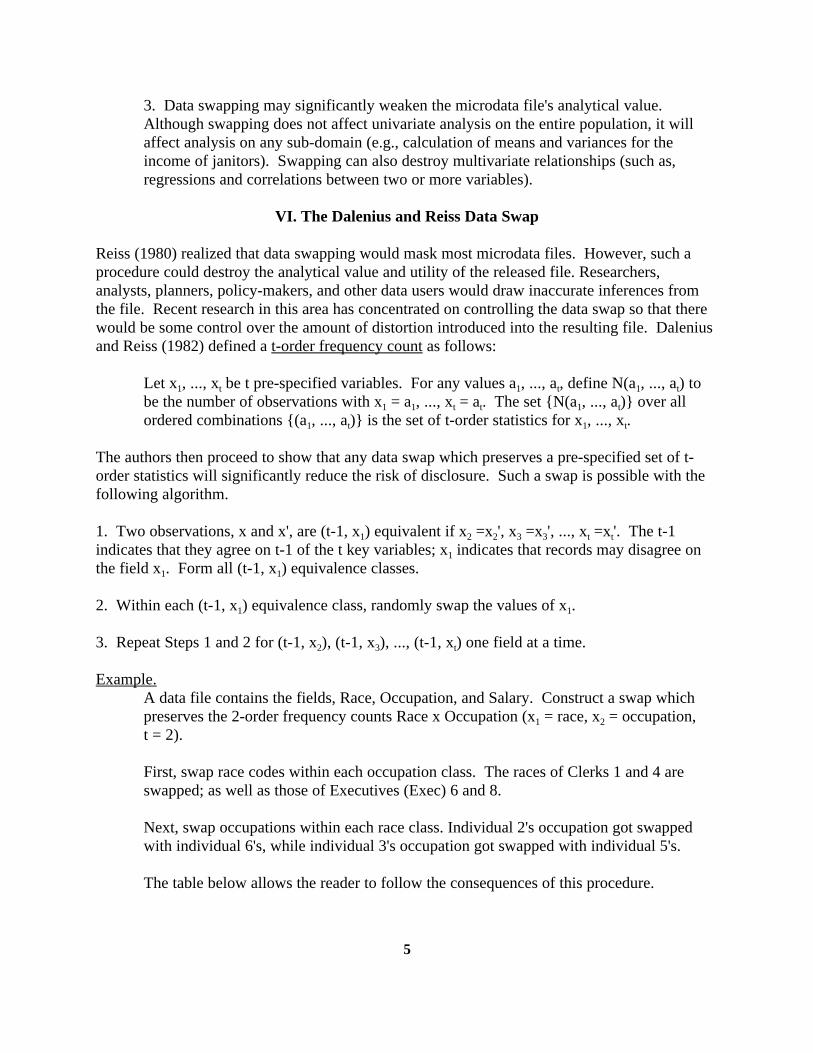
3. Data swapping may significantly weaken the microdata file's analytical value. Although swapping does not affect univariate analysis on the entire population, it willaffect analysis on any sub-domain (e.g., calculation of means and variances for theincome of janitors). Swapping can also destroy multivariate relationships (such as,regressions and correlations between two or more variables).

VI. The Dalenius and Reiss Data Swap

Reiss (1980) realized that data swapping would mask most microdata files. However, such aprocedure could destroy the analytical value and utility of the released file. Researchers,analysts, planners, policy-makers, and other data users would draw inaccurate inferences fromthe file. Recent research in this area has concentrated on controlling the data swap so that therewould be some control over the amount of distortion introduced into the resulting file. Daleniusand Reiss (1982) defined a t-order frequency count as follows:

Let x , ..., x be t pre-specified variables. For any values a , ..., a , define N(a , ..., a ) to1 t 1 t 1 t

be the number of observations with x = a , ..., x = a . The set {N(a , ..., a )} over all1 1 t t 1 t

ordered combinations {(a , ..., a )} is the set of t-order statistics for x , ..., x .1 t 1 t

The authors then proceed to show that any data swap which preserves a pre-specified set of t-order statistics will significantly reduce the risk of disclosure. Such a swap is possible with thefollowing algorithm.

1. Two observations, x and x', are (t-1, x ) equivalent if x =x ', x =x ', ..., x =x '. The t-11 2 2 3 3 t t

indicates that they agree on t-1 of the t key variables; x indicates that records may disagree on1

the field x . Form all (t-1, x ) equivalence classes.1 1

2. Within each (t-1, x ) equivalence class, randomly swap the values of x .1 1

3. Repeat Steps 1 and 2 for (t-1, x ), (t-1, x ), ..., (t-1, x ) one field at a time.2 3 t

Example. A data file contains the fields, Race, Occupation, and Salary. Construct a swap which

preserves the 2-order frequency counts Race x Occupation (x = race, x = occupation, 1 2

t = 2).

First, swap race codes within each occupation class. The races of Clerks 1 and 4 areswapped; as well as those of Executives (Exec) 6 and 8.

Next, swap occupations within each race class. Individual 2's occupation got swappedwith individual 6's, while individual 3's occupation got swapped with individual 5's.

The table below allows the reader to follow the consequences of this procedure.

6

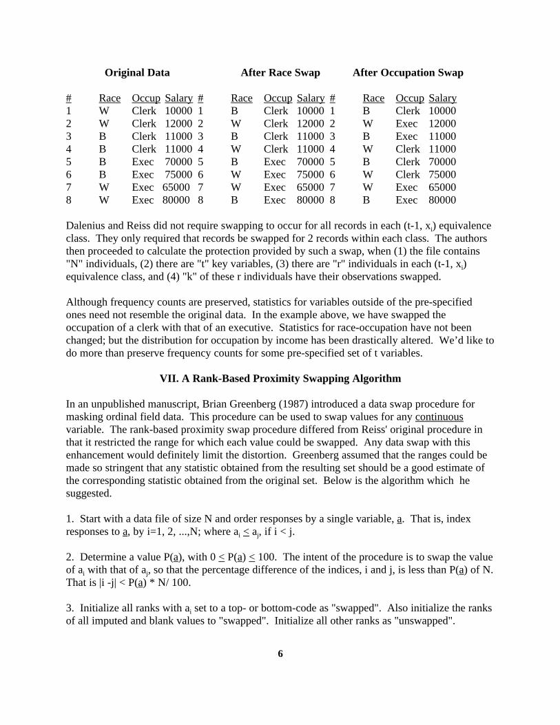
Original Data After Race Swap After Occupation Swap

# Race Occup Salary # Race Occup Salary # Race Occup Salary1 W Clerk 10000 1 B Clerk 10000 1 B Clerk 100002 W Clerk 12000 2 W Clerk 12000 2 W Exec 120003 B Clerk 11000 3 B Clerk 11000 3 B Exec 110004 B Clerk 11000 4 W Clerk 11000 4 W Clerk 110005 B Exec 70000 5 B Exec 70000 5 B Clerk 700006 B Exec 75000 6 W Exec 75000 6 W Clerk 750007 W Exec 65000 7 W Exec 65000 7 W Exec 650008 W Exec 80000 8 B Exec 80000 8 B Exec 80000

Dalenius and Reiss did not require swapping to occur for all records in each (t-1, x ) equivalencei

class. They only required that records be swapped for 2 records within each class. The authorsthen proceeded to calculate the protection provided by such a swap, when (1) the file contains"N" individuals, (2) there are "t" key variables, (3) there are "r" individuals in each (t-1, x )iequivalence class, and (4) "k" of these r individuals have their observations swapped.

Although frequency counts are preserved, statistics for variables outside of the pre-specifiedones need not resemble the original data. In the example above, we have swapped theoccupation of a clerk with that of an executive. Statistics for race-occupation have not beenchanged; but the distribution for occupation by income has been drastically altered. We’d like todo more than preserve frequency counts for some pre-specified set of t variables.

VII. A Rank-Based Proximity Swapping Algorithm

In an unpublished manuscript, Brian Greenberg (1987) introduced a data swap procedure formasking ordinal field data. This procedure can be used to swap values for any continuousvariable. The rank-based proximity swap procedure differed from Reiss' original procedure inthat it restricted the range for which each value could be swapped. Any data swap with thisenhancement would definitely limit the distortion. Greenberg assumed that the ranges could bemade so stringent that any statistic obtained from the resulting set should be a good estimate ofthe corresponding statistic obtained from the original set. Below is the algorithm which hesuggested.

1. Start with a data file of size N and order responses by a single variable, a. That is, indexresponses to a, by i=1, 2, ...,N; where a < a , if i < j.i j

2. Determine a value P(a), with 0 < P(a) < 100. The intent of the procedure is to swap the valueof a with that of a , so that the percentage difference of the indices, i and j, is less than P(a) of N. i j

That is |i -j| < P(a) * N/ 100.

3. Initialize all ranks with a set to a top- or bottom-code as "swapped". Also initialize the ranksi

of all imputed and blank values to "swapped". Initialize all other ranks as "unswapped".

7

4. Let j be the lowest unswapped rank, randomly select a record with an unswapped rank fromthe interval [j+1, M] where M= min {N, j + (P(a)*N/100)}. Suppose the randomly selectedrecord has rank k.

5. Swap the values a and a . Set the labels on these to ranks to "swapped".j k

6. Return to Step 4 and continue until all ranks are labelled "swapped".

7. Suppose one swaps on several additional fields, b, c, ... . Return to Step 1 and repeat theprocedure one field at a time. First use field b, then field c, ... . P(b) need not equal P(a).

8. When the swap is complete, calculate and compare multivariate statistics. If they are notwithin a suitable range, repeat the procedure using smaller values for P(a), and/or P(b), ... .

Greenberg stopped short of guaranteeing that such a swap would preserve statistics within anacceptable error. Methods, proposed in this paper, extend rank-based proximity swap idea. Weconstruct suitable sets from which each swap can occur. The resulting set preserves multivariatestatistics within a suitable statistical error.

VIII. Enhancing the Rank-Based Proximity Swap Algorithm

The remainder of this paper concentrates on enhancing the Rank-Based Proximity SwapAlgorithm. The research focuses on finding a methodology for specifying suitable values forP(a), P(b), ... prior to the initial swap. Before proceeding, determine which statistics must bepreserved, then concentrate on the preservation of the following two conditions:

1. Preservation of Multivariate Dependence/Independence. Let R(a, b) = originalcorrelation between the values in fields a and fields b. Let R(a', b') = the correlationbetween the two fields after swapping. Given an 0.0 < R < 1.0, swap so that 0

E[ R(a', b')] = R * R(a, b).0

Even under controlled conditions, a random swap will destroy some of the naturaldependence between any two fields. Hence, R must be less than 1.0. One definitely0

does not want R < 0.0, otherwise he has reversed the correlation between the fields (i.e.,0

positively correlated fields would appear to be negatively correlated and vice-versa).

2. Preservation of Means of Subsets Which Contain a Large Number of Observations. Asecond desirable property of the swap is to preserve most univariate statistics (e.g.,means, variances, skewness). This is particularly important for subsets which contain alarge number of observations. Researchers may draw conclusions based on subsets of themicrodata file. They are skeptical of inferences based on a small number ofobservations. This skepticism diminishes as the size of the subset increases. The easiestsuch statistic to preserve is the mean. Given K > 0.0, we would like to construct a swap0

so that if a is swapped with a , theni' i

(X&2(K

0(X

N,X%

2(K0(X

N)

8

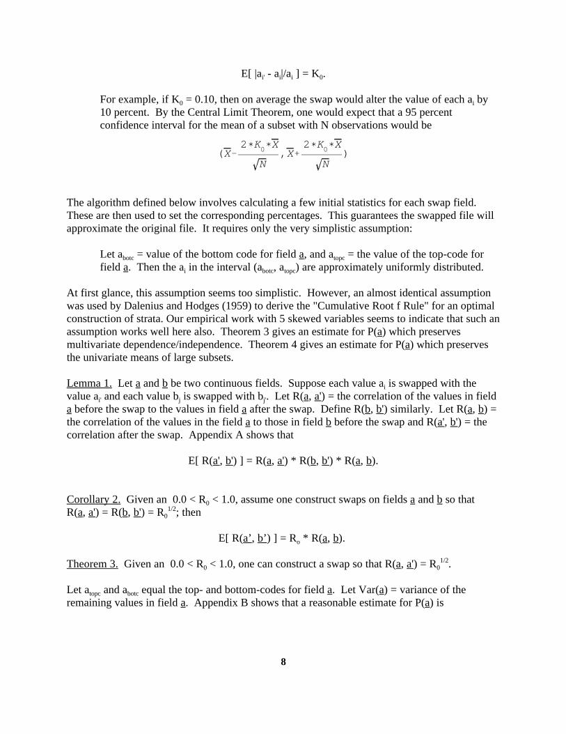
E[ |a - a |/a ] = K .i' i i 0

For example, if K = 0.10, then on average the swap would alter the value of each a by0 i

10 percent. By the Central Limit Theorem, one would expect that a 95 percentconfidence interval for the mean of a subset with N observations would be

The algorithm defined below involves calculating a few initial statistics for each swap field.These are then used to set the corresponding percentages. This guarantees the swapped file willapproximate the original file. It requires only the very simplistic assumption:

Let a = value of the bottom code for field a, and a = the value of the top-code forbotc topc

field a. Then the a in the interval (a , a ) are approximately uniformly distributed.i botc topc

At first glance, this assumption seems too simplistic. However, an almost identical assumptionwas used by Dalenius and Hodges (1959) to derive the "Cumulative Root f Rule" for an optimalconstruction of strata. Our empirical work with 5 skewed variables seems to indicate that such anassumption works well here also. Theorem 3 gives an estimate for P(a) which preservesmultivariate dependence/independence. Theorem 4 gives an estimate for P(a) which preservesthe univariate means of large subsets.

Lemma 1. Let a and b be two continuous fields. Suppose each value a is swapped with thei

value a and each value b is swapped with b . Let R(a, a') = the correlation of the values in fieldi' j j'

a before the swap to the values in field a after the swap. Define R(b, b') similarly. Let R(a, b) =the correlation of the values in the field a to those in field b before the swap and R(a', b') = thecorrelation after the swap. Appendix A shows that

E[ R(a', b') ] = R(a, a') * R(b, b') * R(a, b).

Corollary 2. Given an 0.0 < R < 1.0, assume one construct swaps on fields a and b so that0

R(a, a') = R(b, b') = R ; then01/2

E[ R(a’, b’) ] = R * R(a, b). o

Theorem 3. Given an 0.0 < R < 1.0, one can construct a swap so that R(a, a') = R . 0 01/2

Let a and a equal the top- and bottom-codes for field a. Let Var(a) = variance of thetopc botc

remaining values in field a. Appendix B shows that a reasonable estimate for P(a) is

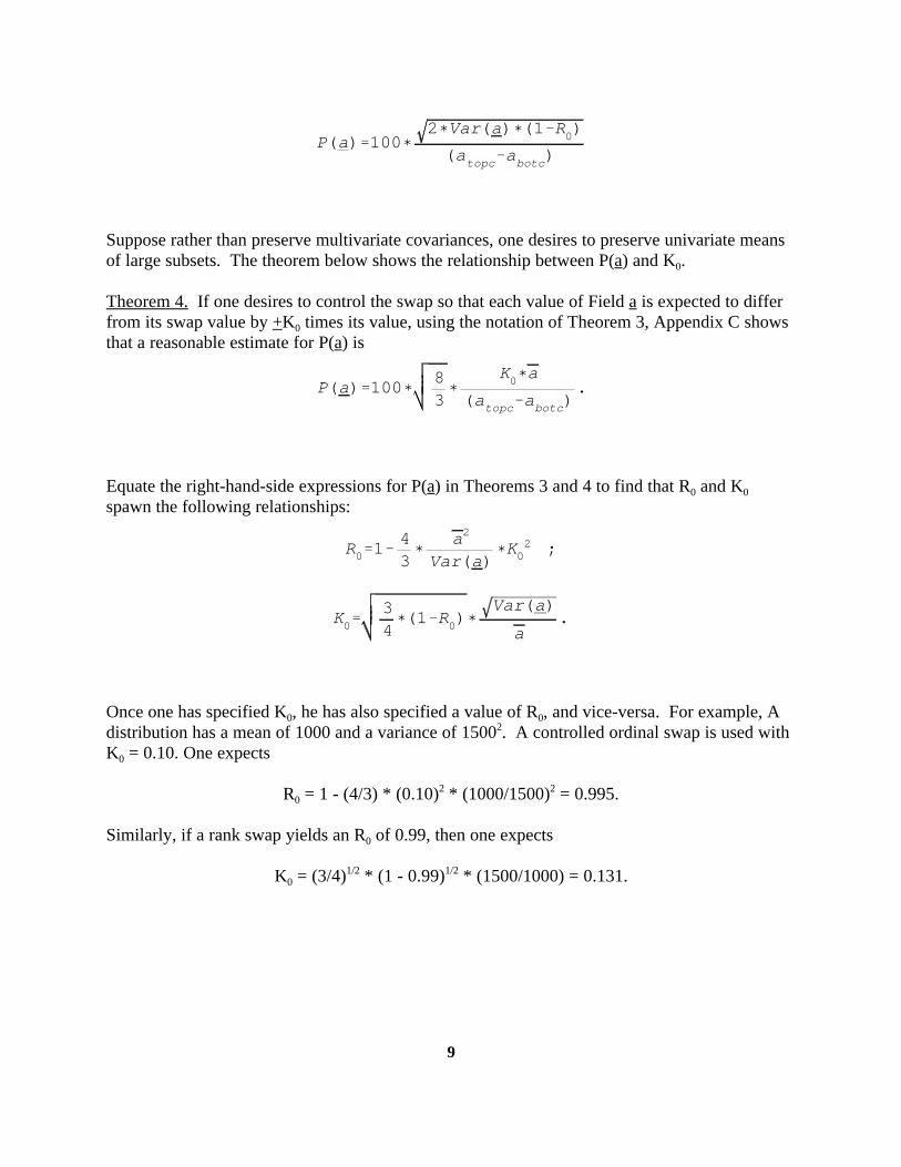
P(a)'100(2(Var(a)((1&R

0)

(atopc&abotc)

P(a)'100(83(

K0(a

(atopc&abotc).

R0'1&43(

a2

Var(a)(K0

2 ;

K0'

34((1&R

0)(

Var(a)

a.

9

Suppose rather than preserve multivariate covariances, one desires to preserve univariate meansof large subsets. The theorem below shows the relationship between P(a) and K .0

Theorem 4. If one desires to control the swap so that each value of Field a is expected to differfrom its swap value by +K times its value, using the notation of Theorem 3, Appendix C shows0

that a reasonable estimate for P(a) is

Equate the right-hand-side expressions for P(a) in Theorems 3 and 4 to find that R and K0 0

spawn the following relationships:

Once one has specified K , he has also specified a value of R , and vice-versa. For example, A0 0

distribution has a mean of 1000 and a variance of 1500 . A controlled ordinal swap is used with2

K = 0.10. One expects 0

R = 1 - (4/3) * (0.10) * (1000/1500) = 0.995.02 2

Similarly, if a rank swap yields an R of 0.99, then one expects0

K = (3/4) * (1 - 0.99) * (1500/1000) = 0.131.01/2 1/2

10

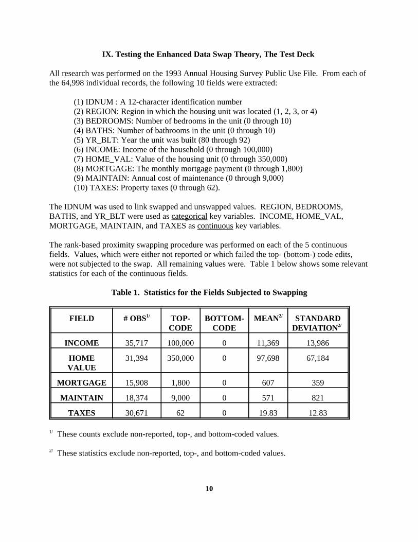
IX. Testing the Enhanced Data Swap Theory, The Test Deck

All research was performed on the 1993 Annual Housing Survey Public Use File. From each ofthe 64,998 individual records, the following 10 fields were extracted:

(1) IDNUM : A 12-character identification number(2) REGION: Region in which the housing unit was located (1, 2, 3, or 4) (3) BEDROOMS: Number of bedrooms in the unit (0 through 10)(4) BATHS: Number of bathrooms in the unit (0 through 10)(5) YR_BLT: Year the unit was built (80 through 92)(6) INCOME: Income of the household (0 through 100,000)(7) HOME_VAL: Value of the housing unit (0 through 350,000)(8) MORTGAGE: The monthly mortgage payment (0 through 1,800)(9) MAINTAIN: Annual cost of maintenance (0 through 9,000)(10) TAXES: Property taxes (0 through 62).

The IDNUM was used to link swapped and unswapped values. REGION, BEDROOMS,BATHS, and YR_BLT were used as categorical key variables. INCOME, HOME_VAL,MORTGAGE, MAINTAIN, and TAXES as continuous key variables.

The rank-based proximity swapping procedure was performed on each of the 5 continuousfields. Values, which were either not reported or which failed the top- (bottom-) code edits,were not subjected to the swap. All remaining values were. Table 1 below shows some relevantstatistics for each of the continuous fields.

Table 1. Statistics for the Fields Subjected to Swapping

FIELD # OBS TOP- BOTTOM- MEAN STANDARD1/

CODE CODE DEVIATION

2/

2/

INCOME 35,717 100,000 0 11,369 13,986

HOME 31,394 350,000 0 97,698 67,184VALUE

MORTGAGE 15,908 1,800 0 607 359

MAINTAIN 18,374 9,000 0 571 821

TAXES 30,671 62 0 19.83 12.83

These counts exclude non-reported, top-, and bottom-coded values.1/

These statistics exclude non-reported, top-, and bottom-coded values.2/

11

X. Objectives of the Rank-Based Proximity Swap

Retention of the Covariate Relationships. This study's primary objective is to show that one isable to control the swap. The masking agent wants to swap values so that the univariate andcovariate properties of the universe are retained. He uses a swapping procedure which retains allof the universe's univariate distributions. Unfortunately, this procedure destroys some of theintrinsic bivariate relationships. One hypothesizes that for a given value of R , 0 < R < 1, he0 0

can control the ranges from Fields a and b, on which he performs the random swaps. Heconstructs these ranges so that the expected post-swap correlation of values in a and b is assumedto be R times the value of the original correlation, (i.e., R(a', b') = R * R(a, b)). The goal is to0 0

demonstrate that, by using this method, one can come close to his correlation, R(a', b').).

Control Within Each Continuous Field. The project has several secondary objectives. If onehas achieved his target correlation, R(a', b'), has he done so by controlling the distortion withineach field? The test must confirm three conjectures. First, there exists a relationship of thepercentage of the total number of records in each swapping interval, P(a), with the desiredcorrelation of the swapped value with its original, R(a, a'). Second, there is also a relationship ofP(a) with K , the average expected absolute percentage difference of the swapped value with the0

original. Third, R(a, a') is a good predictor of K , and vice-versa. 0

Feasibility of Implementation. Another objective examines the logistical feasibility ofimplementing such a swap. The procedure must be relatively easy to program. Programs mustbe written so that they can be readily modified for different variables and microdata files. Theprograms must also execute in a reasonable amount of time.

Masking Ability. A final objective examines the amount of distortion necessary to adequatelymask the data. How is the amount of protection related to R or K ? We can use matching0 0

software developed by Winkler (1995) to determine the percentage of records in any maskedfile, which can be re-identified.

XI. Results of the Testing

Retention of the Covariate Relationships. Testing reveals that the swapping method generallyyields covariances within an acceptable range of their targets. In Table 2, the pre-swap original,post-swap target, and post-swap observed correlation coefficients for the 10 bivariatecombinations of fields swapped are listed. Values correspond to the factor R = 0.975. One0

obtains the values in "POST-SWAP EXP" column by multiplying the corresponding value in the"PRE-SWAP" column by a factor of 0.975. Compare these to the actual post-swap correlationcoefficients displayed in the final column.

12

Table 2. Comparison of the Observed with Expected Correlation CoefficientsFor a Data Swap with Factor, R = 0.975 0

CORRELATION COEFFICIENTS

FIELD a FIELD b # PRE- POST- POST-OBSERV SWAP SWAP SWAPATIONS EXP. OBS.1/

INCOME HOME VAL 23,318 0.150 0.146 0.141

INCOME MORTGAGE 11,225 0.034 0.032 0.024

INCOME MAINTAIN 14,058 0.050 0.049 0.045

INCOME TAXES 22,791 0.095 0.093 0.087

HOME_VAL MORTGAGE 15,514 0.607 0.592 0.595

HOME_VAL MAINTAIN 17,735 0.202 0.197 0.202

HOME_VAL TAXES 29,871 0.576 0.562 0.567

MORTGAGE MAINTAIN 10,872 0.166 0.162 0.164

MORTGAGE TAXES 15,326 0.511 0.499 0.500

MAINTAIN TAXES 17,487 0.167 0.163 0.168

Number of Records on which FIELD a and FIELD b both contained a reported value that fell1/

between the corresponding bottom- and top-code range.

In Table 2, all expected covariances differ from the observed post-swap by less than 0.008.There are only three combinations (HOME_VAL/MORTGAGE, HOME_VAL/TAXES, andTAXES/MORTGAGE) which have a correlation over 0.500. The swapping algorithm does anexcellent job of hitting its target correlation for these combinations. These three combinationsare of the most interest to data-users, since it seems frivolous to do regression analysis onindependent variables. The swap achieves its objective. It preserves bivariate independence andreduces the correlation of highly dependent variables by a pre-defined factor of R .0

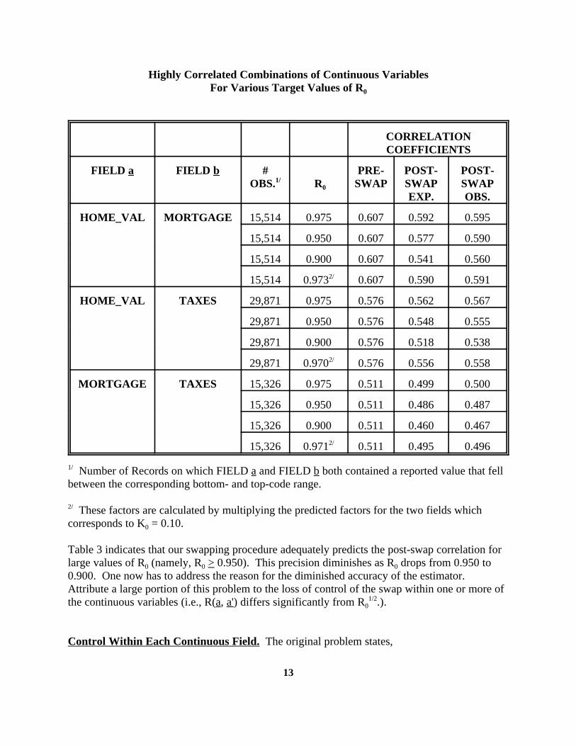
Use Table 3 to compare the expected values to observed post-swap correlations for theHOME_VAL/MORTGAGE, HOME_VAL/TAXES, and MORTGAGE/TAXES combinations. The listed values correspond to R = 0.975, 0.950, and 0.900. Expected post-swap correlations0

are also calculated for these combinations when a swap is constructed to yield an averageabsolute percentage difference of 10 percent (i.e., K = 0.10). In the latter instance, the target0

factor R is calculated by multiplying the correlation (corresponding to K = 0.10 (See Theorem0 0

4.)) for FIELD a with the corresponding correlation for FIELD b (i.e., R = R(a, a') * R(b, b')). 0

Table 3. Observed versus Expected Correlation Coefficients of

13

Highly Correlated Combinations of Continuous VariablesFor Various Target Values of R0

CORRELATIONCOEFFICIENTS

FIELD a FIELD b # PRE- POST- POST-OBS. R SWAP SWAP SWAP1/

0

EXP. OBS.

HOME_VAL MORTGAGE 15,514 0.975 0.607 0.592 0.595

15,514 0.950 0.607 0.577 0.590

15,514 0.900 0.607 0.541 0.560

15,514 0.973 0.607 0.590 0.5912/

HOME_VAL TAXES 29,871 0.975 0.576 0.562 0.567

29,871 0.950 0.576 0.548 0.555

29,871 0.900 0.576 0.518 0.538

29,871 0.970 0.576 0.556 0.5582/

MORTGAGE TAXES 15,326 0.975 0.511 0.499 0.500

15,326 0.950 0.511 0.486 0.487

15,326 0.900 0.511 0.460 0.467

15,326 0.971 0.511 0.495 0.4962/

Number of Records on which FIELD a and FIELD b both contained a reported value that fell1/

between the corresponding bottom- and top-code range.

These factors are calculated by multiplying the predicted factors for the two fields which2/

corresponds to K = 0.10.0

Table 3 indicates that our swapping procedure adequately predicts the post-swap correlation forlarge values of R (namely, R > 0.950). This precision diminishes as R drops from 0.950 to0 0 0

0.900. One now has to address the reason for the diminished accuracy of the estimator. Attribute a large portion of this problem to the loss of control of the swap within one or more ofthe continuous variables (i.e., R(a, a') differs significantly from R .).0

1/2

Control Within Each Continuous Field. The original problem states,

14

"Given R , can we determine appropriate values of P(a) and P(b), (i.e., the maximum0

number of observations in each swapping set)?"

One "solves" this problem by constructing appropriate percentages based on R . If the expected0

value of the post-swap correlation, R(a', b'), differs significantly from the original correlationdiminished by a factor of R (i.e., R * R(a, b)), then the problem may occur in one of the0 0

following three assumptions:

(1) E[ R(a', b') ] = R * R(a, b);0

(2) Theorem 3 does not adequately estimate P(a) for certain values of R ; or0

(3) Theorem 3 does not adequately estimate P(b) for certain values of R .0

See Appendix A for a proof that Assumption (1) holds. The results of Tables 2 and 3 alsosupport this. Let's concentrate attention to the validity of P(a) and P(b). Recall that theconstruction of P(a) hinges on one simple, but very crucial, assumption, "The values of Field aare uniformly distributed between the bottom- and top-code for a." How uniform are thesedistributions?"

All five of these continuous variables are skewed. In uniform distributions, the standarddeviation would be approximately 28 percent of the interval length. Use Table 1 to calculatethese ratios for each field. They are approximately

INCOME .............. 14 percent,HOME VALUE ... 18 percent,MORTGAGE ....... 20 percent,MAINTAIN ........... 9 percent, andTAXES ................. 21 percent.

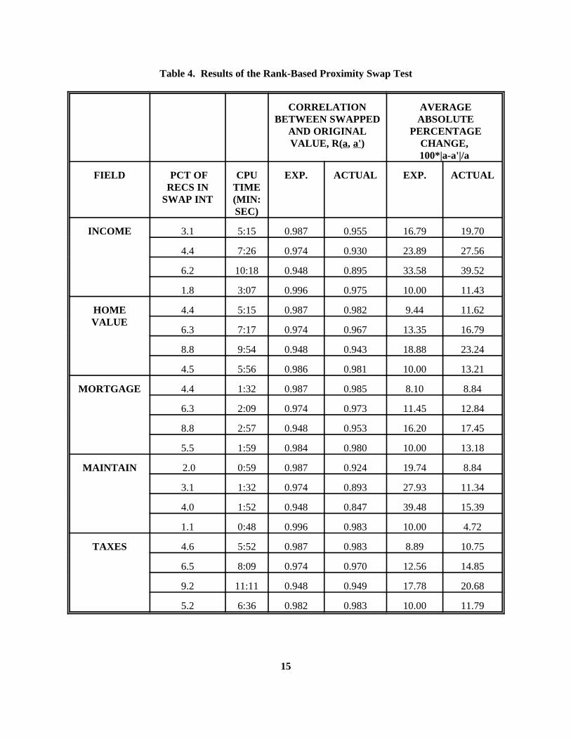
The most highly skewed fields are INCOME and MAINTAIN; while the other three arerelatively uniform. Expect P(a) to be a worse approximation of interval length for MAINTAINthan for TAXES. Table 4 confirms this. Suppose one desires a target correlation of theswapped to the unswapped value of 0.987. For MORTGAGE, TAXES, and HOME VALUE,this method yields correlations which fall between 0.982 and 0.985. Notice the observed post-swap correlations for the other variables. INCOME has a post-swap correlation of 0.955, whileMAINTAIN has one of 0.924. One cannot dismiss the importance of a distribution's skewness. Should he abandon this hypothesis, since it was based on an erroneous assumption?

For "near uniform" distributions, the theory does a good job of estimating P(a) for large valuesof R . Yet it fails as R decreases. Examine the proofs in Appendix B. It is very important that0 0

the distribution be nearly uniform on each swapping interval. The range of the swappinginterval increases as R decreases. For values of R near 1.00, the ranges will be very small and0 0

15

Table 4. Results of the Rank-Based Proximity Swap Test

CORRELATION AVERAGEBETWEEN SWAPPED ABSOLUTE

AND ORIGINAL PERCENTAGEVALUE, R(a, a') CHANGE,

100*|a-a'|/a

FIELD PCT OF CPU EXP. ACTUAL EXP. ACTUALRECS IN TIME

SWAP INT (MIN:SEC)

INCOME 3.1 5:15 0.987 0.955 16.79 19.70

4.4 7:26 0.974 0.930 23.89 27.56

6.2 10:18 0.948 0.895 33.58 39.52

1.8 3:07 0.996 0.975 10.00 11.43

HOME 4.4 5:15 0.987 0.982 9.44 11.62VALUE

6.3 7:17 0.974 0.967 13.35 16.79

8.8 9:54 0.948 0.943 18.88 23.24

4.5 5:56 0.986 0.981 10.00 13.21

MORTGAGE 4.4 1:32 0.987 0.985 8.10 8.84

6.3 2:09 0.974 0.973 11.45 12.84

8.8 2:57 0.948 0.953 16.20 17.45

5.5 1:59 0.984 0.980 10.00 13.18

MAINTAIN 2.0 0:59 0.987 0.924 19.74 8.84

3.1 1:32 0.974 0.893 27.93 11.34

4.0 1:52 0.948 0.847 39.48 15.39

1.1 0:48 0.996 0.983 10.00 4.72

TAXES 4.6 5:52 0.987 0.983 8.89 10.75

6.5 8:09 0.974 0.970 12.56 14.85

9.2 11:11 0.948 0.949 17.78 20.68

5.2 6:36 0.982 0.983 10.00 11.79

16

distribution will be "almost" uniform of most swapping intervals. As R decreases, the intervals0

become bigger and less uniform.

For highly-skewed distributions, P(a) can be accurately determined only at relatively high valuesof R . For INCOME, R = 0.975 (R(a, a') = R = 0.987) is too low. For less-skewed0 0 0

1/2

distributions, such as TAXES, R = 0.900 and R(a, a') = 0.948 give remarkably good estimates. 0

A good topic for future research will be the quantitative relationship between the skewness ofthe distribution and the ability of R to give an accurate prediction of the appropriate number of0

percentage of the total number of observations in a swapping interval, P(a).

Recall that K is the average percentage change induced by the rank swap. Table 4 shows that0

the theory provides good predictions for the relationship between K and P(a). Again, the0

distribution of each swapping interval is assumed to be approximately uniform. For relativelysmall swapping intervals, the K -estimator is an extremely good predictor. It even compensates0

for a "moderately" skewed distribution such as INCOME (Target K = 10, Observed K =0 0

11.43). However, for very extremely skewed distributions, such as MAINTAIN, even the K0

estimator fails miserably (Target K = 10.00, Observed K = 4.72.). As the theory predicts, P(a)0 0

and the observed value of K are directly proportional. Compare values (within each field) of0

the "PCT OF RECORDS IN SWAPPING INTERVAL" column with the "AVERAGEABSOLUTE PCT CHANGE/ OBS."column from Table 4. The columns are almost directlylinearly correlated. When P(a) doubles, the observed value of K approximately doubles.0

Also use Table 4 to confirm the inverse relationship between the observed correlation, R(a, a')and the corresponding observed value of K . This is a logical consequence of the validity of0

Theorems 3 and 4. For pre-defined values of K which correspond to values of R near 1.000 0

(e.g., R > 0.95), one can construct a sampling interval for which the observed correlation is near0

the target. For less skewed distributions, values for this corresponding R can extend to 0.9000

and lower. The theory holds. Is implementing such a swap feasible?

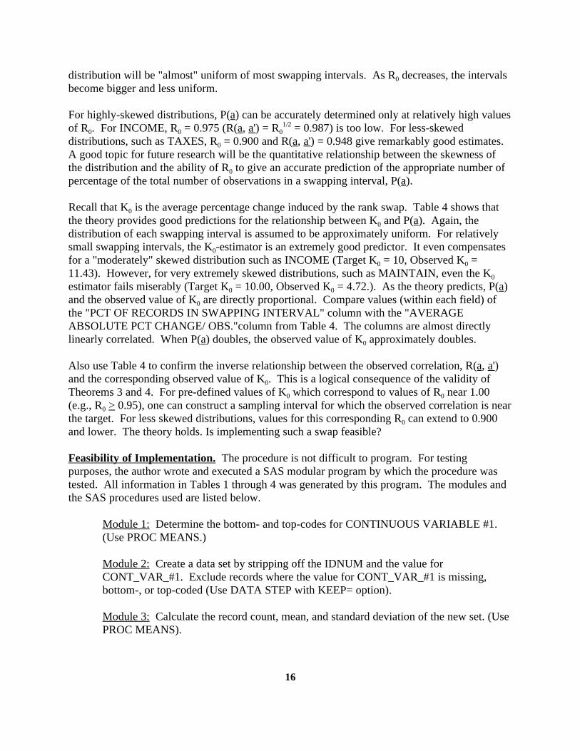
Feasibility of Implementation. The procedure is not difficult to program. For testingpurposes, the author wrote and executed a SAS modular program by which the procedure wastested. All information in Tables 1 through 4 was generated by this program. The modules andthe SAS procedures used are listed below.

Module 1: Determine the bottom- and top-codes for CONTINUOUS VARIABLE #1. (Use PROC MEANS.)

Module 2: Create a data set by stripping off the IDNUM and the value forCONT_VAR_#1. Exclude records where the value for CONT_VAR_#1 is missing,bottom-, or top-coded (Use DATA STEP with KEEP= option).

Module 3: Calculate the record count, mean, and standard deviation of the new set. (UsePROC MEANS).

17

Module 4: Sort the data set by CONT_VAR_#1. (Use PROC SORT.)

Module 5: Swap the data. (Use a DATA step.) This is the only module which requiressome involved programming. It also requires the most Central Processing Unit (CPU)time to execute. In this program, the user sets the following parameters:

(1) Record Count of the set,(2) Target Factors, R and K ,0 0

(3) Mean of CONT_VAR_#1,(4) Standard Deviation of CONT_VAR_#1,(5) Bottom-code of CONT_VAR_#1, and(6) Top-code of CONT_VAR_#1.

The program (1) calculates P(a), by use of a programmed formula,(2) chooses an appropriate random number,(3) randomly swaps the data in the prescribed manner, and(4) sets the swap flags.

Module 6: Sort the output set of the previous module by IDNUM. (Use PROC SORT.)

Repeat Modules 1 through 6 for CONT_VAR_#2, CONT_VAR_#3, ... .Module 7: Combine all information from the output sets of Module 6. (Use DATA stepwith a MERGE BY IDNUM.)

Module 8: Analyze the correlation coefficients of the continuous variables after theswap. (Use PROC CORR on the set produced in Module 7.)

Module 9: Produce the correlation coefficients for the original set (Use PROC CORR onthe original set.) Manually compare the two. (For files with a large number ofcontinuous variables, use PROC COMPARE.)

If the user is satisfied with the results of the swap, invoke Module 10.

Module 10: Update the values of continuous variables. (Use a DATA step withUPDATE statement

Even though the code for Module 5 is the most difficult to write, it is extremely easy tomodify. The user can easily change any combination of the following.

(1) To execute for a different value of the Diminishing Factor, R (or K ), reset0 0

the value of the parameter R and re-execute the program.0

(2) To execute for a different continuous variable, change the parmeters: setcount, mean, standard deviation, bottom-, and top-code. Re-execute.

CPU for ai(sec.)' N(ai)((P(ai)

4%

13000

);

CPU for Total Swap(sec.)'jk

i'1N(ai)((

P(ai)

4%

13000

).

18

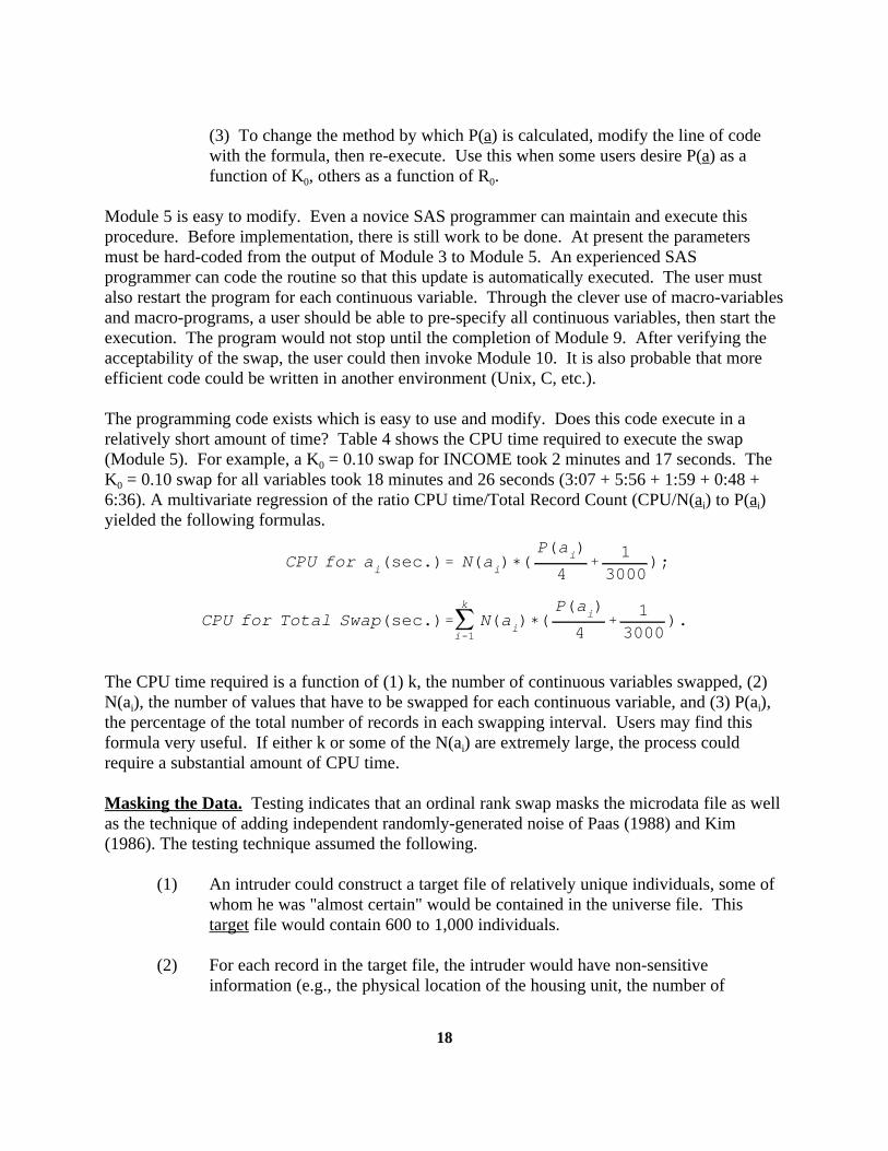
(3) To change the method by which P(a) is calculated, modify the line of codewith the formula, then re-execute. Use this when some users desire P(a) as afunction of K , others as a function of R . 0 0

Module 5 is easy to modify. Even a novice SAS programmer can maintain and execute thisprocedure. Before implementation, there is still work to be done. At present the parametersmust be hard-coded from the output of Module 3 to Module 5. An experienced SASprogrammer can code the routine so that this update is automatically executed. The user mustalso restart the program for each continuous variable. Through the clever use of macro-variablesand macro-programs, a user should be able to pre-specify all continuous variables, then start theexecution. The program would not stop until the completion of Module 9. After verifying theacceptability of the swap, the user could then invoke Module 10. It is also probable that moreefficient code could be written in another environment (Unix, C, etc.).

The programming code exists which is easy to use and modify. Does this code execute in arelatively short amount of time? Table 4 shows the CPU time required to execute the swap(Module 5). For example, a K = 0.10 swap for INCOME took 2 minutes and 17 seconds. The0

K = 0.10 swap for all variables took 18 minutes and 26 seconds (3:07 + 5:56 + 1:59 + 0:48 +0

6:36). A multivariate regression of the ratio CPU time/Total Record Count (CPU/N(a ) to P(a ) i i

yielded the following formulas.

The CPU time required is a function of (1) k, the number of continuous variables swapped, (2)N(a ), the number of values that have to be swapped for each continuous variable, and (3) P(a ),i i

the percentage of the total number of records in each swapping interval. Users may find thisformula very useful. If either k or some of the N(a ) are extremely large, the process couldi

require a substantial amount of CPU time.

Masking the Data. Testing indicates that an ordinal rank swap masks the microdata file as wellas the technique of adding independent randomly-generated noise of Paas (1988) and Kim(1986). The testing technique assumed the following.

(1) An intruder could construct a target file of relatively unique individuals, some ofwhom he was "almost certain" would be contained in the universe file. Thistarget file would contain 600 to 1,000 individuals.

(2) For each record in the target file, the intruder would have non-sensitiveinformation (e.g., the physical location of the housing unit, the number of

19

bathrooms and bedrooms which it contained, and the year in which it was built),which he believed to be very reliable. The intruder is slightly skeptical aboutcertain values in some of these non-sensitive fields.

(3) For each targeted observation, the intruder was also able to make reasonablyaccurate guesses (within 10 percent of the true value for five sensitive items(household income, home value, mortgage payment, annual maintenance, andproperty taxes).

(4) Because the intruder has accurate information on non-sensitive items, he canrestrict the universe to less than 20,000 observations.

(5) The intruder has a very sophisticated matching software program. The softwarewill link each record from the target file to the "most likely" match in therestricted universe. The intruder has a pre-defined criteria for which linkages aredefinitely re-identifications, which are suspect, and which are not re-identifications. For definite re-identifications, it is important to the intruder thathe obtain accurate information for all five of the sensitive values. The intrudermay realize that the values in the restricted universe have been perturbed, but hedoes not know to what extent.

(6) The intruder has sufficient knowledge of the software, and the target, andrestricted universe files to accurately set the required matching parameters.

The Restricted Universe. The intruder first constructs the restricted universe by blocking theobservations into equivalence classes. Two observations are in the same equivalence class ifthey contain the same values for BATHS, BEDROOMS, YR_BUILT, and REGION. Restrictthe universe to only those classes with less than 100 observations. This would produce a file of18,557 observations.

The Target File. The intruder's target file contains all observations in the equivalence classeswith 2 or less observations. This file contained 771 observations.

Introduction of Some Intruder Skepticism. After the construction of the target and restricteduniverse files, the intruder becomes skeptical of certain values in the non-sensitive variables. Without reconstructing either file, he decides to collapse certain equivalence classes. For(programming) simplicity, assume the region code was inaccurate. Collapse these filesaccordingly. Two records are now equivalent, if they contain the same values for BATHS,BEDROOMS, and YR_BLT. The target file now has equivalence class blocks containing 7 orless observations. The restricted universe has blocks containing 213 (as compared to 100) orfewer records.

20

The Matching Software. The intruder has software which utilizes the matching algorithmdeveloped by Fellegi and Sunter (1969). He also posesses software similar to that of Winkler(1988), he can calculate a reasonably matching and non-matching "weights" for the sensitivevariables.

The Expectation-Maximization (EM) software of Winkler (1988) obtains good estimates for aset of weights, which would do the best job re-identifying the true corresponding record in therestricted universe. This software independently compares values of each variable in the targetfile to the corresponding variable in the universe.

If the typical value of that variable has a large number of possible matches in the universe, theEM algorithm assigns a variable a low positive weight for matching cases. If the typical value inthat field has a limited number of possible matches, it assigns a large positive value. Negativeweights are assigned for mismatch weights. Large negative numbers indicate that there are alimited number of possible mismatches for the typical value. Small negative weights, indicatethat the typical value has many possible mismatches.

In our testing, we have access to a unique identifier, which is attached to each record in thetarget and universe files. Thus, we are able to positively determine whether the weights were theoptimal for discrimination. In actuality, the intruder would not have this information availableto him. He would derive a less optimal set of weights, this would cause more "definite" re-identifications, which were incorrect. Weights will differ between the perturbed versions of theuniverse. Fortunately, for the intruder, the optimal weights did not differ significantly from theform of perturbation used. Table 5 gives the approximate optimal weights.

The Fellegi-Sunter routine independently matches each field on the target file to records on therestricted universe file. This match is restricted to those records in the universe which have thesame values as the key variables (BATHS, BEDROOM, YR_BLT) of the target file. Theappropriate positive/negative weight from Table 5 is obtained for each variable. Each record inthe universe is assigned a value equal to the sum of the 5 weights (one weight for each sensitivefield). The record in the universe with the largest aggregate weight is linked to the target.

Table 5 shows that HOME VALUE is a good discriminator of true re-identification. For thetypical value of HOME VALUE, there are a limited number of cases which are possible matchesand non-matches. INCOME, on the other hand, is a less adequate discriminator. For the typicalINCOME value, there are many possible matches and mismatches.

Criteria for Definite, Suspect, and Erroneous Re-identifications. The intruder is interested inaccurately identifying all five sensitive values. If one of the five is suspect, he questions the re-identification. In addition, if two or more of the values are suspect, he dismisses the linkage as acase for which no suitable match is found.

If the sum is greater than +10.0, then all five fields match within 10 percent of the intruder'sexpectation. In this case, he assumes that he has a positive re-identification.

21

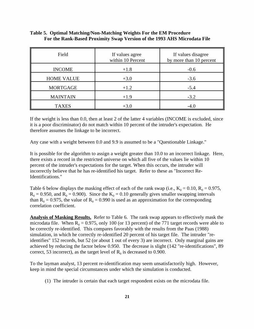
Table 5. Optimal Matching/Non-Matching Weights For the EM ProcedureFor the Rank-Based Proximity Swap Version of the 1993 AHS Microdata File

Field If values agree If values disagree within 10 Percent by more than 10 percent

INCOME +1.8 -0.6

HOME VALUE +3.0 -3.6

MORTGAGE +1.2 -5.4

MAINTAIN +1.9 -3.2

TAXES +3.0 -4.0

If the weight is less than 0.0, then at least 2 of the latter 4 variables (INCOME is excluded, sinceit is a poor discriminator) do not match within 10 percent of the intruder's expectation. Hetherefore assumes the linkage to be incorrect.

Any case with a weight between 0.0 and 9.9 is assumed to be a "Questionable Linkage."

It is possible for the algorithm to assign a weight greater than 10.0 to an incorrect linkage. Here,there exists a record in the restricted universe on which all five of the values lie within 10percent of the intruder's expectations for the target. When this occurs, the intruder willincorrectly believe that he has re-identified his target. Refer to these as "Incorrect Re-Identifications."

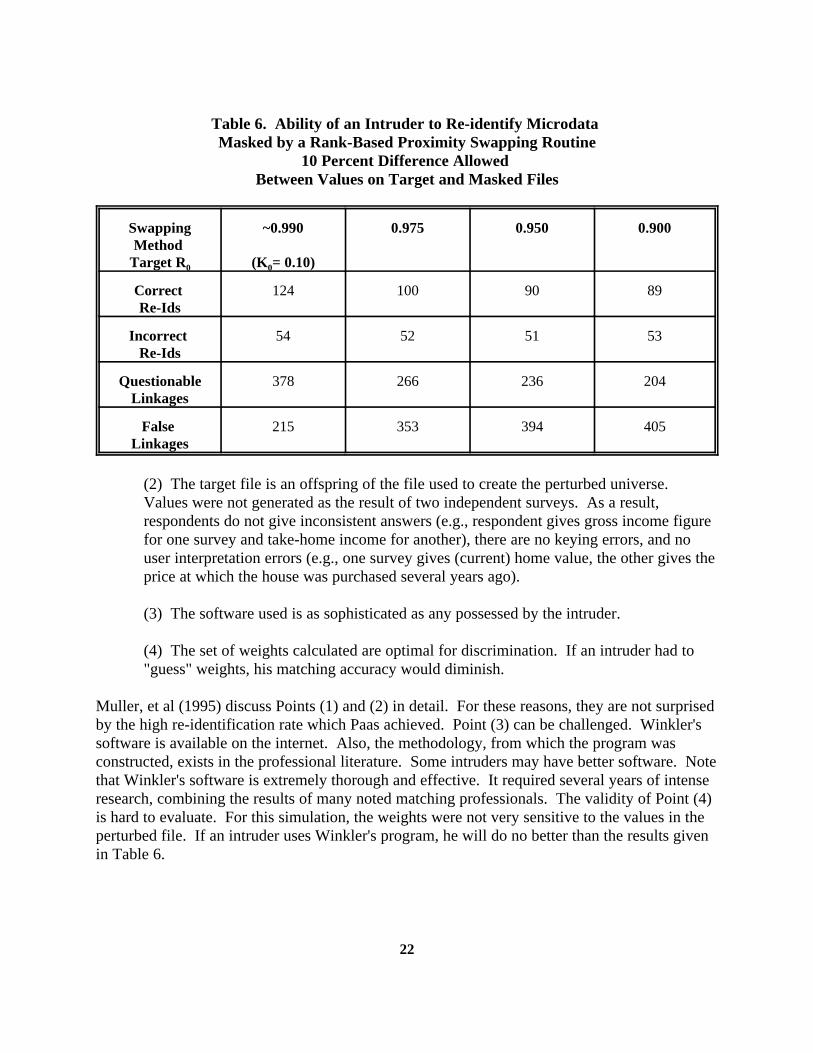
Table 6 below displays the masking effect of each of the rank swap (i.e., K = 0.10, R = 0.975,0 0

R = 0.950, and R = 0.900). Since the K = 0.10 generally gives smaller swapping intervals0 0 0

than R = 0.975, the value of R = 0.990 is used as an approximation for the corresponding0 0

correlation coefficient.

Analysis of Masking Results. Refer to Table 6. The rank swap appears to effectively mask themicrodata file. When R = 0.975, only 100 (or 13 percent) of the 771 target records were able to0

be correctly re-identified. This compares favorably with the results from the Paas (1988)simulation, in which he correctly re-identified 20 percent of his target file. The intruder "re-identifies" 152 records, but 52 (or about 1 out of every 3) are incorrect. Only marginal gains areachieved by reducing the factor below 0.950. The decrease is slight (142 "re-identifications", 89correct, 53 incorrect), as the target level of R is decreased to 0.900. 0

To the layman analyst, 13 percent re-identification may seem unsatisfactorily high. However,keep in mind the special circumstances under which the simulation is conducted.

(1) The intruder is certain that each target respondent exists on the microdata file.

22

Table 6. Ability of an Intruder to Re-identify Microdata Masked by a Rank-Based Proximity Swapping Routine

10 Percent Difference Allowed Between Values on Target and Masked Files

Swapping ~0.990 0.975 0.950 0.900Method

Target R (K = 0.10)0 0

Correct 124 100 90 89Re-Ids

Incorrect 54 52 51 53Re-Ids

Questionable 378 266 236 204Linkages

False 215 353 394 405Linkages

(2) The target file is an offspring of the file used to create the perturbed universe. Values were not generated as the result of two independent surveys. As a result,respondents do not give inconsistent answers (e.g., respondent gives gross income figurefor one survey and take-home income for another), there are no keying errors, and nouser interpretation errors (e.g., one survey gives (current) home value, the other gives theprice at which the house was purchased several years ago).

(3) The software used is as sophisticated as any possessed by the intruder.

(4) The set of weights calculated are optimal for discrimination. If an intruder had to"guess" weights, his matching accuracy would diminish.

Muller, et al (1995) discuss Points (1) and (2) in detail. For these reasons, they are not surprisedby the high re-identification rate which Paas achieved. Point (3) can be challenged. Winkler'ssoftware is available on the internet. Also, the methodology, from which the program wasconstructed, exists in the professional literature. Some intruders may have better software. Notethat Winkler's software is extremely thorough and effective. It required several years of intenseresearch, combining the results of many noted matching professionals. The validity of Point (4)is hard to evaluate. For this simulation, the weights were not very sensitive to the values in theperturbed file. If an intruder uses Winkler's program, he will do no better than the results givenin Table 6.

23

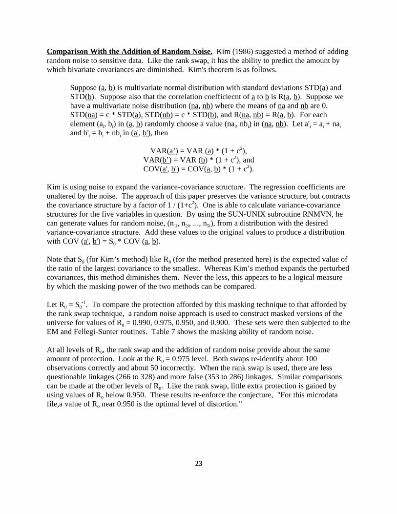
Comparison With the Addition of Random Noise. Kim (1986) suggested a method of addingrandom noise to sensitive data. Like the rank swap, it has the ability to predict the amount bywhich bivariate covariances are diminished. Kim's theorem is as follows.

Suppose (a, b) is multivariate normal distribution with standard deviations STD(a) andSTD(b). Suppose also that the correlation coefficiecnt of a to b is R(a, b). Suppose wehave a multivariate noise distribution (na, nb) where the means of na and nb are 0,STD(na) = c * STD(a), STD(nb) = c * STD(b), and R(na, nb) = R(a, b). For eachelement (a , b ) in (a, b) randomly choose a value (na , nb ) in (na, nb). Let a' = a + nai i i i i i i

and b' = b + nb in (a', b'), theni i i

VAR(a’) = VAR (a) * (1 + c ),2

VAR(b’) = VAR (b) * (1 + c ), and2

COV(a', b') = COV(a, b) * (1 + c ).2

Kim is using noise to expand the variance-covariance structure. The regression coefficients areunaltered by the noise. The approach of this paper preserves the variance structure, but contractsthe covariance structure by a factor of 1 / (1+c ). One is able to calculate variance-covariance2

structures for the five variables in question. By using the SUN-UNIX subroutine RNMVN, hecan generate values for random noise, (n , n , ..., n ), from a distribution with the desired1i 2i 5i

variance-covariance structure. Add these values to the original values to produce a distributionwith COV (a', b') = S * COV (a, b).0

Note that S (for Kim’s method) like R (for the method presented here) is the expected value of0 0

the ratio of the largest covariance to the smallest. Whereas Kim’s method expands the perturbedcovariances, this method diminishes them. Never the less, this appears to be a logical measureby which the masking power of the two methods can be compared.

Let R = S . To compare the protection afforded by this masking technique to that afforded by0 0-1

the rank swap technique, a random noise approach is used to construct masked versions of theuniverse for values of R = 0.990, 0.975, 0.950, and 0.900. These sets were then subjected to the0

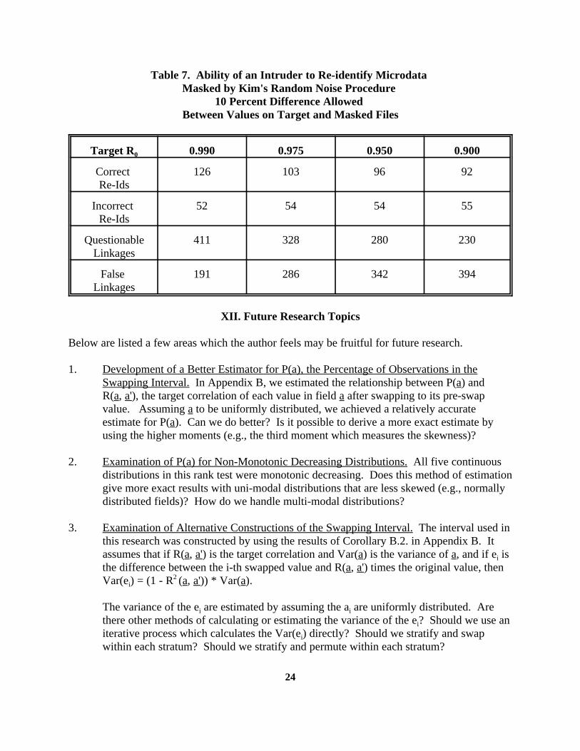
EM and Fellegi-Sunter routines. Table 7 shows the masking ability of random noise. At all levels of R , the rank swap and the addition of random noise provide about the same0

amount of protection. Look at the R = 0.975 level. Both swaps re-identify about 1000

observations correctly and about 50 incorrectly. When the rank swap is used, there are lessquestionable linkages (266 to 328) and more false (353 to 286) linkages. Similar comparisonscan be made at the other levels of R . Like the rank swap, little extra protection is gained by0

using values of R below 0.950. These results re-enforce the conjecture, "For this microdata0

file,a value of R near 0.950 is the optimal level of distortion."0

24

Table 7. Ability of an Intruder to Re-identify Microdata Masked by Kim's Random Noise Procedure

10 Percent Difference Allowed Between Values on Target and Masked Files

Target R 0.990 0.975 0.950 0.9000

Correct 126 103 96 92Re-Ids

Incorrect 52 54 54 55Re-Ids

Questionable 411 328 280 230Linkages

False 191 286 342 394Linkages

XII. Future Research Topics

Below are listed a few areas which the author feels may be fruitful for future research.

1. Development of a Better Estimator for P(a), the Percentage of Observations in theSwapping Interval. In Appendix B, we estimated the relationship between P(a) and R(a, a'), the target correlation of each value in field a after swapping to its pre-swapvalue. Assuming a to be uniformly distributed, we achieved a relatively accurateestimate for P(a). Can we do better? Is it possible to derive a more exact estimate byusing the higher moments (e.g., the third moment which measures the skewness)?

2. Examination of P(a) for Non-Monotonic Decreasing Distributions. All five continuousdistributions in this rank test were monotonic decreasing. Does this method of estimationgive more exact results with uni-modal distributions that are less skewed (e.g., normallydistributed fields)? How do we handle multi-modal distributions?

3. Examination of Alternative Constructions of the Swapping Interval. The interval used inthis research was constructed by using the results of Corollary B.2. in Appendix B. Itassumes that if R(a, a') is the target correlation and Var(a) is the variance of a, and if e isi

the difference between the i-th swapped value and R(a, a') times the original value, thenVar(e ) = (1 - R (a, a')) * Var(a).i

2

The variance of the e are estimated by assuming the a are uniformly distributed. Arei i

there other methods of calculating or estimating the variance of the e ? Should we use ani

iterative process which calculates the Var(e ) directly? Should we stratify and swapi

within each stratum? Should we stratify and permute within each stratum?

25

4. Development of a Rank Swap for Categorical Variables. The rank swap works well forcontinuous variables because they can be sorted in ascending or descending order. Isthere some analogous method to rank categorical variables? Should we attempt todevelop a metric from R to R ; use this metric on the n sensitive continuous variables ton 1

stratify the microdata file; then swap categorical variables within stratum? Should wefirst block all categorical variables, then swap entire blocks?

5. Analysis of a Rank Swap on Statistics of Sub-Domains. This research shows that there isa "predictable" relationship between R and K . In Section VIII, it was hypothesized that0 0

bias of the mean of a subset was directly proportional to K . No simulations were done0

to prove or disprove this conjecture. The author's "gut" feeling is that the conjecture istrue for random subsets. It probably does not hold for non-randomly constructed subsets(e.g., houses with more than 8 bathrooms, or units valued over $250,000). Can wequantify the bias as a function of K and the frequency with which each observation (in0

the subset in question) appears in the universe?

6. Development of Intruder Simulation Software. Paas (1985), Winkler (1988, 1995), andFienberg, et al. (1995) have developed matching software. All used the software to re-identify individual respondents in "masked" data sets. We used Winkler's software tosimulate an intruder in this project. Is our model reasonable? Should we set up someguidelines and develop the software to simulate a sophisticated intruder? Whatconstitutes a reasonable target set? What constitutes a re-identification? Whatpercentage of re-identifications are tolerable for a public use file?

XIII. Conclusions

The technological revolution of the 1980s has allowed data-users to handle larger and moredetailed data sets than ever before. This has been accompanied by the public's easy access tovery sophisticated matching software. As a result, government agencies have been compelled torelease only microdata files with very limited detail. Severe restrictions have been placed on thesampling fraction of the universe, the amount of geographic detail, and the range of values forcontinuous data released. Users have found this extremely irritating and unacceptable.

Data swapping appears to be a feasible alternative to severe top- and bottom-codes. Thistechnique was first suggested by Reiss in the early 1980s, and has evolved significantly. In thepast, the Bureau has shied away from its use. It has been argued that it not only masks the file,but also diminishes its multivariate analytical utility. This paper illustrates that an effectiveversion of the data swap exists which controls the amount of distortion induced.

The Bureau has used the addition of random noise to mask microdata files. This also distorts thedata in a "controlled" manner. Both techniques measure the amount of distortion by comparingthe bivariate covariances of the data after the swap to the corresponding values before the swap. For a pre-specified amount of distortion, this research shows that data-swapping protectsindividuals identities as well as (if not better than) the addition of random noise.

26

In addition, the data-swapping technique suggested here should be relatively quick to code andeasy to modify and enhance. Testing has shown that, under reasonable circumstances, it doesnot take a long time to execute. For files with many sensitive continuous fields, or those with alarge number of observations, this routine may require too much computer resources. However,a formula has been provided from which a reasonable estimate of the expected number of CPUseconds (on a VAX cluster) can be obtained.

Should the Bureau consider rank swapping a potentially feasible method to mask microdata files,there is a plethora of directions in which the research can proceed. These range from improvingour estimates for the appropriate swapping interval to the development of an intruder model.

This method is quick, has the ability to control the distortion, and masks the data well. Istrongly urge the Bureau to consider implementation of this technique to limit the risk ofdisclosure in future public use microdata files.

XIV. References

1. Cochran, W. (1977). Sampling Techniques (3rd edition), New York: John Wiley andSons.

2. Dalenius, T. and Hodges, J. L. Jr. (1959). Minimum Variance Stratification. Journal ofAmerican Statistical Association 54, 88-101.

3. Dalenius, T. and Reiss, S. P. (1982). Data-swapping: A Technique for DisclosureControl. Journal of Statistical Planning and Inference 6, 73-85.

4. Feinberg, S. E., Makov, U. E., and Sanil, A. P. (1995). A Bayesian Approach to DataDisclosure: Optimal Intruder Behavior for Continuous Data. Bureau of the CensusContract 50-YABC-2-66205, Task Order 8, Activity 1.

5. Fellegi, I. P. and Sunter, A. B. (1969). A Theory of Record Linkage, Journal of theAmerican Statistical Association, 64, 1183-1210.

6. Greenberg, B. (1987), Rank Swapping for Masking Ordinal Microdata, US Bureau of theCensus (unpublished manuscript).

7. Greenberg, B. and Voshell, L. (1990). The Geographic Component of Disclosure Riskfor Microdata. Statistical Research Division Report Series Census/SRD/RR-90/13, USBureau of the Census.

8. Kim, J. J. (1986). A Method For Limiting Disclosure in Microdata Based on RandomNoise and Transformation. Proceedings of Survey Research Methods Section, AmericanStatistical Association, 303-308.

27

9. Muller, W., Blien, U., and Wirth, H. (1995), Identification Risks of Microdata,Sociological Methods and Research, 24, 131-157.

10. Paas, G. (1988). Disclosure Risk and Disclosure Avoidance for Microdata, Journal ofBusiness and Economic Statistics, 6, 487-500.

11. Reiss, S. P. (1980). Practical Data-Swapping: The First Steps, IEEE Symposium onSecurity and Privacy, 38-43.

12. Subcommittee on Statistical Disclosure Limitation Methodology of the FederalCommittee on Statistical Methodology (1994). Report on Statistical DisclosureLimitation Methodology, Statistical Policy Working Paper 22, Office of Manangementand Budget, Washington, DC.

13. Winkler, W. E. (1988). Using the EM Algorithm for Weight Computation in the Fellegi-Sunter Model of Record Linkage, Proceedings of the Survey Research Methods Section,American Statistical Association, 667-671.

14. Winkler, W. E. (1995). Matching and Record Linkage, in Business Survey Methods,(Cox, B.G., ed) New York: John Wiley and Sons, 355-384.

j e 2i,

(1)j ei((ai&a)'0,(2)j ei'0.

z'j e 2i'j (bi&m(ai&c)

2.

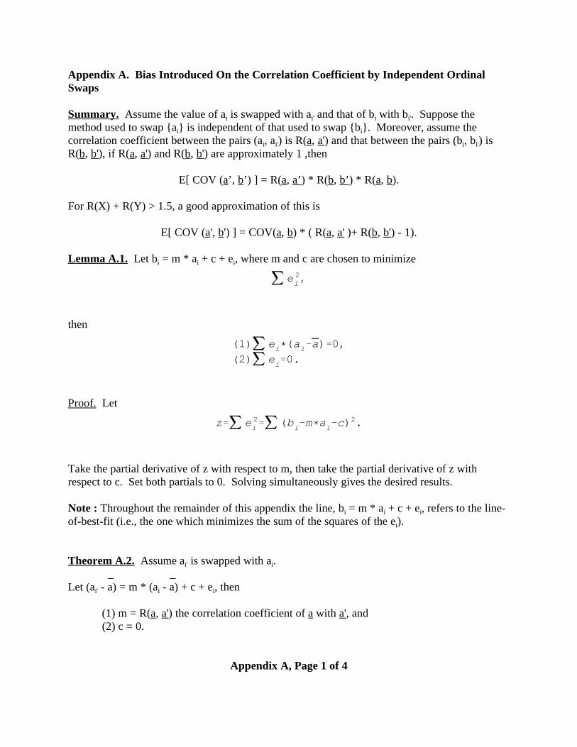
Appendix A. Bias Introduced On the Correlation Coefficient by Independent OrdinalSwaps

Summary. Assume the value of a is swapped with a and that of b with b . Suppose thei i' i i'

method used to swap {a } is independent of that used to swap {b }. Moreover, assume thei i

correlation coefficient between the pairs (a , a ) is R(a, a') and that between the pairs (b , b ) isi i' i i'

R(b, b'), if R(a, a') and R(b, b') are approximately 1 ,then

E[ COV (a’, b’) ] = R(a, a’) * R(b, b’) * R(a, b).

For R(X) + R(Y) > 1.5, a good approximation of this is

E[ COV (a', b') ] = COV(a, b) * ( R(a, a' )+ R(b, b') - 1).

Lemma A.1. Let b = m * a + c + e , where m and c are chosen to minimize i i i

then

Proof. Let

Take the partial derivative of z with respect to m, then take the partial derivative of z withrespect to c. Set both partials to 0. Solving simultaneously gives the desired results.

Note : Throughout the remainder of this appendix the line, b = m * a + c + e , refers to the line-i i i

of-best-fit (i.e., the one which minimizes the sum of the squares of the e ).i

Theorem A.2. Assume a is swapped with a .i' i

_ _Let (a - a) = m * (a - a) + c + e , theni' i i

(1) m = R(a, a') the correlation coefficient of a with a', and(2) c = 0.

Appendix A, Page 1 of 4

z'j [(ai )&a)&m((ai&a)&c&ei]2.

(zc&2

)'j (ai )&a)

&m(j (ai&a)&c

(zm2n

)'(1n)(j (ai )&a)((ai&a)

&m(( 1n)(j (ai&a)

2

&(cn)(j (ai&a)

R(a ),b)'R(a,a ))(R(a,b)%( 1n)(j ei((bi&b)

Proof. Let

Take the partial with respect to c and divide by -2.

The first two summations on the right-hand side are 0. Since z = 0, this forces c = 0.c

Take the partial of z with respect to m, then divide by 2n.

The last term in the summation is 0. Since z = 0 and c = 0, the first and second terms on them

right-hand side are equal. This implies COV(a, a') = m VAR(a). Divide both of these terms byVAR(a) to get the desired result of R(a, a') = m.

_ _Therefore the line-of-best-fit is (a - a) = R(a, a') * (a - a) + e .i' i i

Theorem A.3. Suppose a is the value swapped for a and that each b is not swapped, theni' i i

Appendix A, Page 2 of 4

R(a ),b)'( 1n)(j (ai )&a)((bi&b)

'(1n)(j [R(a,a ))((ai&a)%ei]((bi&b)

'R(a,a ))(R(a,b)%(1n)(j ei((bi&b)

(ai )&a)'R(a,a ))((ai&a)%ei(bi )&b)'R(b,b ))((bi&b)%fi

R(a ),b ))'R(a,a ))(R(b,b ))(R(a,b)

%(1n)(j ei((bi )&b)%(

1n)(j fi((ai )&a)&(

1n)(j (ei(fi)

R(a ),b ))'[R(a,a ))(R(a,b ))]

%(1n)(j ei((bi )&b)

'[R(a,a ))(R(b,b ))(R(a,b)

%(R(a,a ))

n)(j fi((ai&a)]

%(1n)(j ei((bi )&b).

Setting R(a,a ))((ai&a)'(ai )&a)&eigives the desired result.

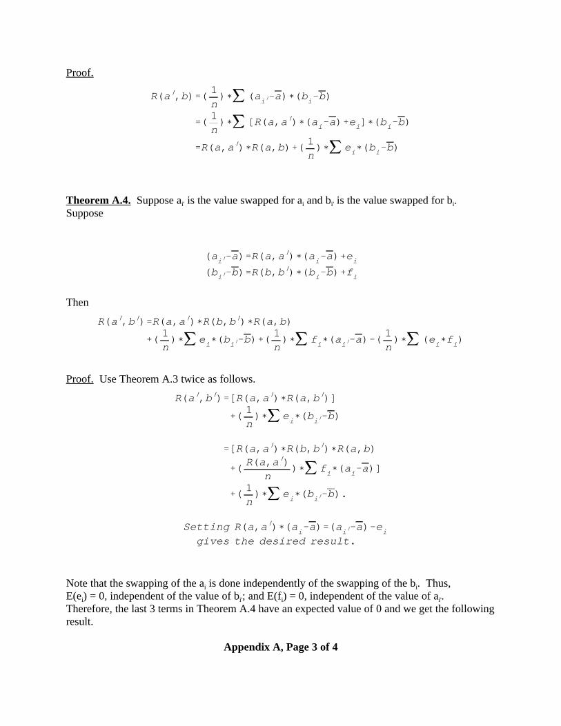
Proof.

Theorem A.4. Suppose a is the value swapped for a and b is the value swapped for b .i' i i' i

Suppose

Then

Proof. Use Theorem A.3 twice as follows.

Note that the swapping of the a is done independently of the swapping of the b . Thus, i i

E(e ) = 0, independent of the value of b ; and E(f ) = 0, independent of the value of a . i i' i i'

Therefore, the last 3 terms in Theorem A.4 have an expected value of 0 and we get the followingresult.

Appendix A, Page 3 of 4

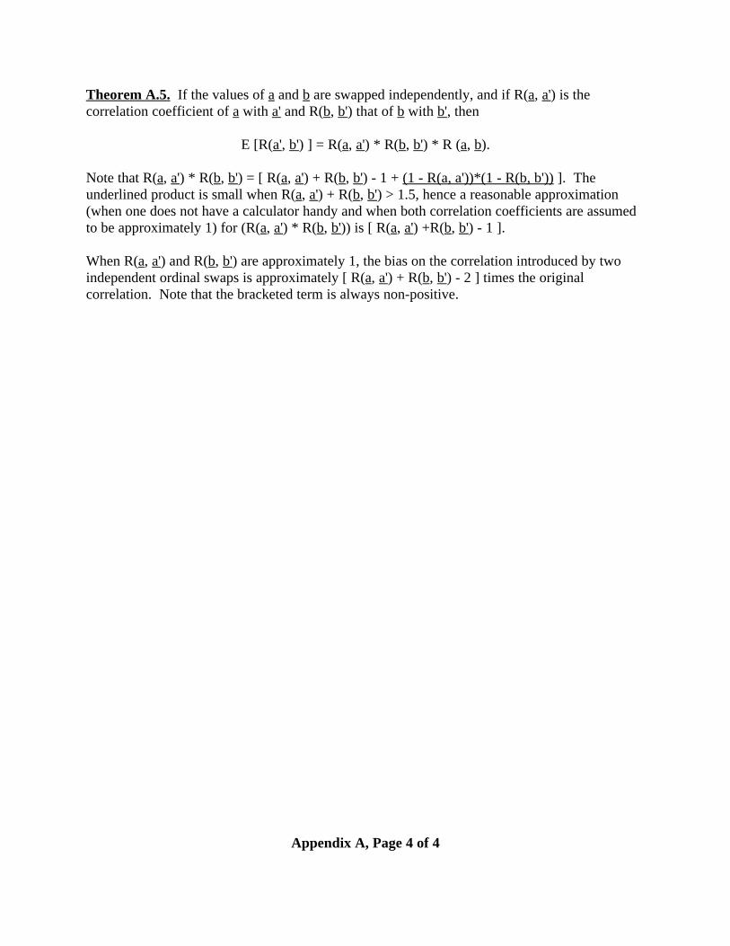
Theorem A.5. If the values of a and b are swapped independently, and if R(a, a') is thecorrelation coefficient of a with a' and R(b, b') that of b with b', then

E [R(a', b') ] = R(a, a') * R(b, b') * R (a, b).

Note that R(a, a') * R(b, b') = [ R(a, a') + R(b, b') - 1 + (1 - R(a, a'))*(1 - R(b, b')) ]. Theunderlined product is small when R(a, a') + R(b, b') > 1.5, hence a reasonable approximation(when one does not have a calculator handy and when both correlation coefficients are assumedto be approximately 1) for (R(a, a') * R(b, b')) is [ R(a, a') +R(b, b') - 1 ].

When R(a, a') and R(b, b') are approximately 1, the bias on the correlation introduced by twoindependent ordinal swaps is approximately [ R(a, a') + R(b, b') - 2 ] times the originalcorrelation. Note that the bracketed term is always non-positive.

Appendix A, Page 4 of 4

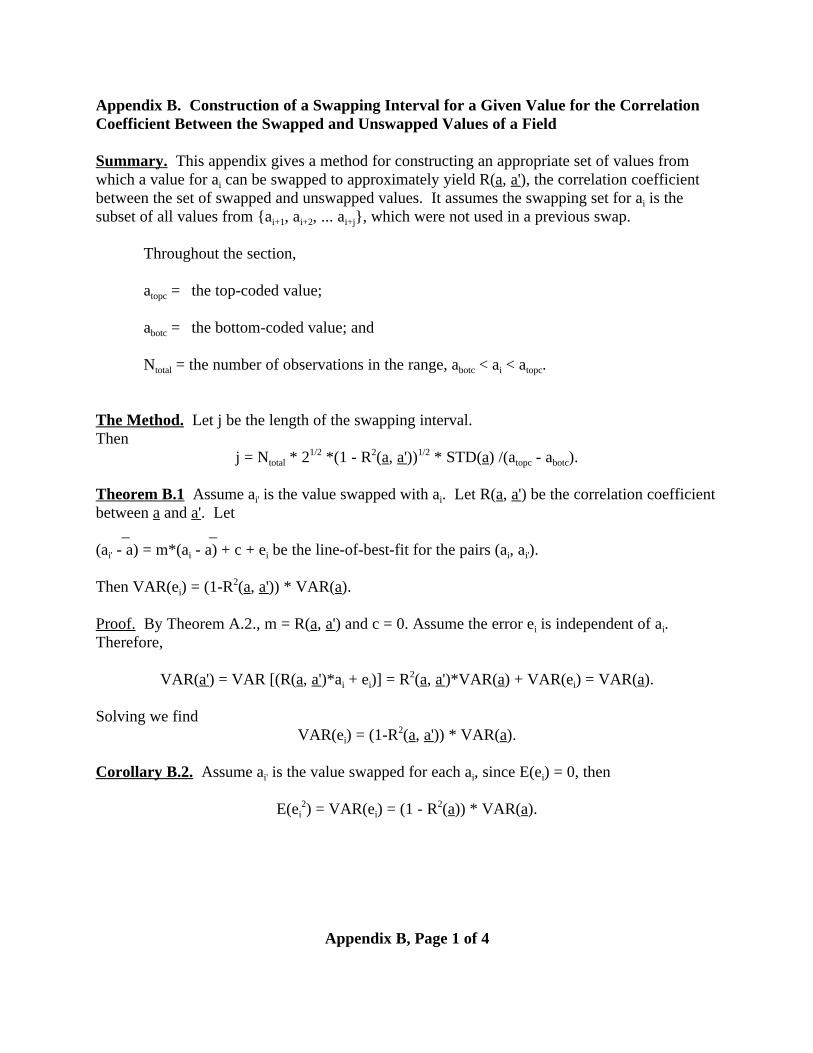
Appendix B. Construction of a Swapping Interval for a Given Value for the CorrelationCoefficient Between the Swapped and Unswapped Values of a Field

Summary. This appendix gives a method for constructing an appropriate set of values fromwhich a value for a can be swapped to approximately yield R(a, a'), the correlation coefficienti

between the set of swapped and unswapped values. It assumes the swapping set for a is thei

subset of all values from {a , a , ... a }, which were not used in a previous swap.i+1 i+2 i+j

Throughout the section,

a = the top-coded value;topc

a = the bottom-coded value; andbotc

N = the number of observations in the range, a < a < a .total botc i topc

The Method. Let j be the length of the swapping interval. Then

j = N * 2 *(1 - R (a, a')) * STD(a) /(a - a ).total topc botc1/2 2 1/2

Theorem B.1 Assume a is the value swapped with a . Let R(a, a') be the correlation coefficienti' i

between a and a'. Let _ _

(a - a) = m*(a - a) + c + e be the line-of-best-fit for the pairs (a , a ).i' i i i i'

Then VAR(e ) = (1-R (a, a')) * VAR(a).i2

Proof. By Theorem A.2., m = R(a, a') and c = 0. Assume the error e is independent of a . i i

Therefore,

VAR(a') = VAR [(R(a, a')*a + e )] = R (a, a')*VAR(a) + VAR(e ) = VAR(a).i i i2

Solving we find VAR(e ) = (1-R (a, a')) * VAR(a).i

2

Corollary B.2. Assume a is the value swapped for each a , since E(e ) = 0, then i' i i

E(e ) = VAR(e ) = (1 - R (a)) * VAR(a).i i2 2

Appendix B, Page 1 of 4

Theorem B.3. An Estimate of s (due to Jim Fagan). Assume that the swapping length is N(a)and the typical swapping set has s elements. Then s ~ 0.75 * N(a).

Proof. Consider the element a . It will be swapped with exactly 1 of 2*N(a) elements in theN(a)+k

set S below.

S = S U S = {a , a , ..., a } U {a , ..., a , a , ..., a }. 1 2 k k+1 N(a)-1 N(a) N(a)+k-1 N(a)+k+1 2*N(a)+k

The set S has N(a) - k elements, and the set S has N(a) + k elements.1 2

Assume after each swap of a , the elements are replaced. Then S for the swap of a will alwaysi i+1

have 2*N(a) elements. Therefore, the probability that a will be swapped from an element inN(a)+k

S is 2

p(k) =(N(a) + k)/ ( 2 * N(a)).

Now calculate the average P(k) for k = 1, 2, ..., N(a). With replacement this average is _p = 3/4 + 1/(4 * N(a)).

Conclusion. With replacement, about 0.75 of the elements in the set {a , ..., a } would bek+1 k+N(a)

swapped with values whose indices are greater than or equal to k.

Therefore, s ~ 0.75 * N(a). We then assume s ~ s .wr wor wr

Table B.4 shows the results for a Monte-Carlo test on the ratio of s to N(a). From this, one mayconclude that s ~ 0.72 * N(a).

Table B.4 Monte Carlo Testing for the Expected Swapping Set Size, s

N(a) s s/N(a)

100 73 0.730

250 180 0.720

500 361 0.722

1000 721 0.721

1500 1082 0.721

2000 1444 0.722

2500 1806 0.722

Appendix B, Page 2 of 4

q(k) '23

((N(a)%k)

(N(a))2.

Theorem B.4 ( due to Moore and Fagan). Assume the set a = {a } is uniformly distributedi

between the range, a to a . Suppose the desired coefficient between the swapped andbotc topc

unswapped values is R(a, a'). Then a reasonable estimation for a p-percent rank swappinginterval is

(P(a) / 100) = (18/7) * (1-R (a, a')) * STD(a)/(a - a ).2 1/2topc botc

Proof. (1) Let N(a) = the maximum number of observations in the swapping intervalof fixed length, then

P(a)/100 = N(a)/N .total

(2) Uniform distribution implies

a = a + d*k, where d = a - a .i+k i i+1 i

(3) The swapping set for a is the set of all unswapped values in { a , a , ...,i i+1 i+2

a }.i+N(a)

(4) Now a may have already been swapped with one of the N(a)-1 membersi+1

of the set {a , ..., a , a }.i-N(a)+1 i-2 i-1

Now a may have already been swapped with one of the N(a)-2 membersi+2

of the set {a , ..., a , a }.i-N(a)+2 i-2 i-1

Now a may have already been swapped with one of the N(a)-k membersi+k

of the set {x , ..., a , a }.i-N(a)+k i-2 i-1

Let p(k) be the probability that a is still in the swap set. From the proofi+k

of Theorem B.3, we see, that

p(k) =(N(a) + k)/ ( 2 * N(a)).

Let q(k) = the probability that the value of a is swapped for the value ofi+k

a . Then q(k) can be estimated by the probability a is still in the swapi i+k

set times the probability that it is selected (i.e., p(k) / E(s)).

From Theorem 3, E(s) ~ (3/4) * N(a), so

Appendix B, Page 3 of 4

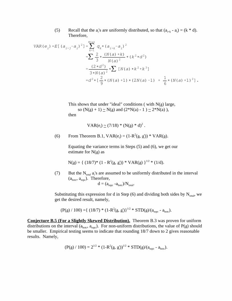
VAR(ei)'E[(ai%j&ai)2]' j

N(a)

k'1qk((ai%k&ai)

2

'j 23((N(a)%k)

N(a)2((k 2(d 2)

'(2(d 2)

3(N(a)2(j [N(a)(k 2%k 3]

'd 2([29((N(a)%1)((2N(a)&1) %

16((N(a)%1)2].

(5) Recall that the a 's are uniformly distributed, so that (a - a ) = (k * d). i i+k i

Therefore,

This shows that under "ideal" conditions ( with N(a) large, so (N(a) + 1) ~ N(a) and (2*N(a) - 1 ) ~ 2*N(a) ),then

VAR(e ) ~ (7/18) * (N(a) * d) .i2

(6) From Theorem B.1, VAR(e ) = (1-R (a, a')) * VAR(a).i2

Equating the variance terms in Steps (5) and (6), we get ourestimate for N(a) as

N(a) = { (18/7)* (1 - R (a, a')) * VAR(a) } * (1/d).2 1/2

(7) But the N a 's are assumed to be uniformly distributed in the interval total i

(a , a ). Therefore,botc topc

d = (a -a )/N .topc botc total

Substituting this expression for d in Step (6) and dividing both sides by N , wetotal

get the desired result, namely,

(P(a) / 100) ={ (18/7) * (1-R (a, a')} * STD(a)/(a - a ).2 1/2topc botc

Conjecture B.5 (For a Slightly Skewed Distribution). Theorem B.3 was proven for uniformdistributions on the interval (a , a ). For non-uniform distributions, the value of P(a) shouldbotc topc

be smaller. Empirical testing seems to indicate that rounding 18/7 down to 2 gives reasonableresults. Namely,

(P(a) / 100) = 2 * (1-R (a, a')) * STD(a)/(a - a ).1/2 2 1/2topc botc

Appendix B, Page 4 of 4

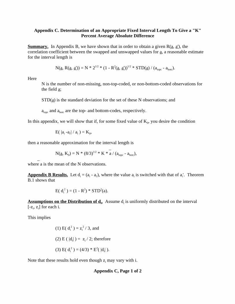
Appendix C. Determination of an Appropriate Fixed Interval Length To Give a "K"Percent Average Absolute Difference

Summary. In Appendix B, we have shown that in order to obtain a given R(a, a'), thecorrelation coefficient between the swapped and unswapped values for a, a reasonable estimatefor the interval length is

N(a, R(a, a')) = N * 2 * (1 - R (a, a')) * STD(a) / (a - a ).1/2 2 1/2topc botc

Here N is the number of non-missing, non-top-coded, or non-bottom-coded observations forthe field a;

STD(a) is the standard deviation for the set of these N observations; and

a and a are the top- and bottom-codes, respectively. topc botc

In this appendix, we will show that if, for some fixed value of K , you desire the condition0

E( |a -a | / a ) = K , i i' i 0

then a reasonable approximation for the interval length is _

N(a, K ) = N * (8/3) * K * a / (a - a ), 0 topc botc1/2

_where a is the mean of the N observations.

Appendix B Results. Let d = (a - a ), where the value a is switched with that of a '. Theoremi i i' i i

B.1 shows that

E( d ) = (1 - R ) * STD (a).i2 2 2

Assumptions on the Distribution of d . Assume d is uniformly distributed on the interval i i

[-z , z ] for each i.i i

This implies

(1) E( d ) = z / 3, and i i2 2

(2) E ( |d | ) = z / 2; thereforei i

(3) E( d ) = (4/3) * E ( |d | ).i i2 2

Note that these results hold even though z may vary with i.i

Appendix C, Page 1 of 2

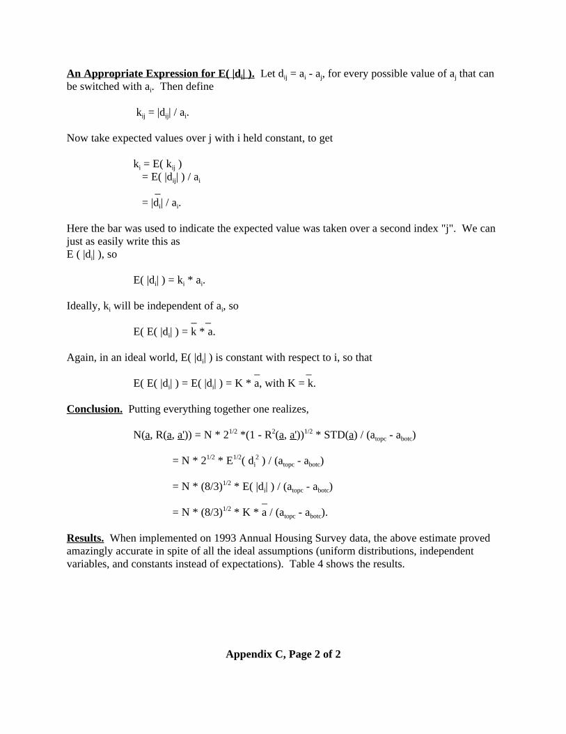
An Appropriate Expression for E( |d | ). Let d = a - a , for every possible value of a that cani ij i j j

be switched with a . Then definei

k = |d | / a .ij ij i

Now take expected values over j with i held constant, to get

k = E( k ) i ij

= E( |d | ) / aij i

_ = |d | / a .i i

Here the bar was used to indicate the expected value was taken over a second index "j". We canjust as easily write this as E ( |d | ), soi

E( |d | ) = k * a .i i i

Ideally, k will be independent of a , soi i

_ _E( E( |d | ) = k * a.i

Again, in an ideal world, E( |d | ) is constant with respect to i, so that i

_ _

E( E( |d | ) = E( |d | ) = K * a, with K = k.i i

Conclusion. Putting everything together one realizes,

N(a, R(a, a')) = N * 2 *(1 - R (a, a')) * STD(a) / (a - a )1/2 2 1/2topc botc

= N * 2 * E ( d ) / (a - a )1/2 1/2 2i topc botc

= N * (8/3) * E( |d | ) / (a - a )1/2i topc botc

_

= N * (8/3) * K * a / (a - a ).1/2topc botc

Results. When implemented on 1993 Annual Housing Survey data, the above estimate provedamazingly accurate in spite of all the ideal assumptions (uniform distributions, independentvariables, and constants instead of expectations). Table 4 shows the results.

Appendix C, Page 2 of 2