Controllable Fluid and Sand Controllable Fluid and Sand SimulationSimulation

Controllable Fluid and Sand Controllable Fluid and Sand SimulationSimulation

Yizhou Yu Department of Computer Science

University of Illinois at Urbana-Champaign

Yizhou Yu Department of Computer Science

University of Illinois at Urbana-Champaign

Controllable Smoke Simulation with Controllable Smoke Simulation with Guiding ObjectsGuiding ObjectsControllable Smoke Simulation with Controllable Smoke Simulation with Guiding ObjectsGuiding Objects

• Amorphous but elegantly moving matters, such as clouds, fog and smoke, give people space for imagination.

• Develop techniques for digitally reproducing similar effects. Such techniques have applications in advertising and film making.

• Amorphous but elegantly moving matters, such as clouds, fog and smoke, give people space for imagination.

• Develop techniques for digitally reproducing similar effects. Such techniques have applications in advertising and film making.

Shi and Yu, ACM Transactions on Graphics, 2005

ObjectivesObjectivesObjectivesObjectives

• The motion during two-way transitions between irregular smoke regions and regular object shapes should be natural and have realistic smoke appearances;

• The global shape of the smoke should be able to approximate a static or moving object for an arbitrarily long period of time while maintaining its characteristic local structure and motion;

• When smoke objects interact with each other or with the environment, the objects should exhibit the properties of smoke so that a strong wind or other regular objects can easily destroy the shape of such objects.

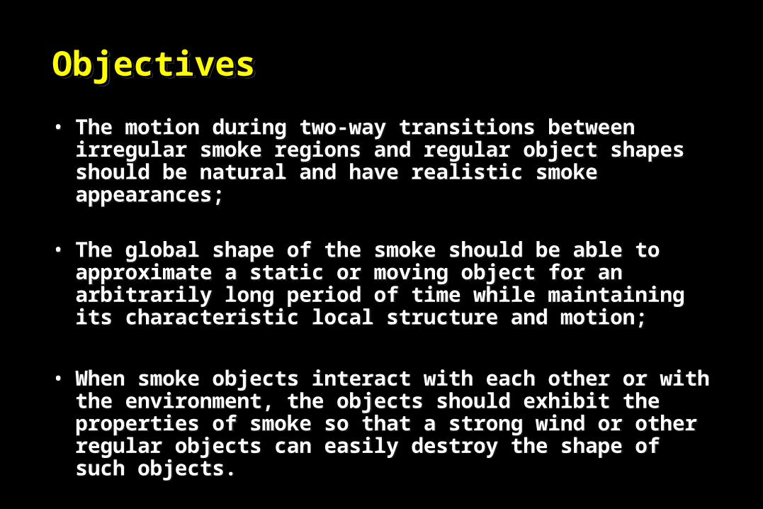
• The motion during two-way transitions between irregular smoke regions and regular object shapes should be natural and have realistic smoke appearances;

• The global shape of the smoke should be able to approximate a static or moving object for an arbitrarily long period of time while maintaining its characteristic local structure and motion;

• When smoke objects interact with each other or with the environment, the objects should exhibit the properties of smoke so that a strong wind or other regular objects can easily destroy the shape of such objects.

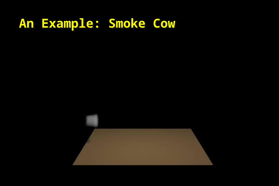
An Example: Smoke CowAn Example: Smoke CowAn Example: Smoke CowAn Example: Smoke Cow

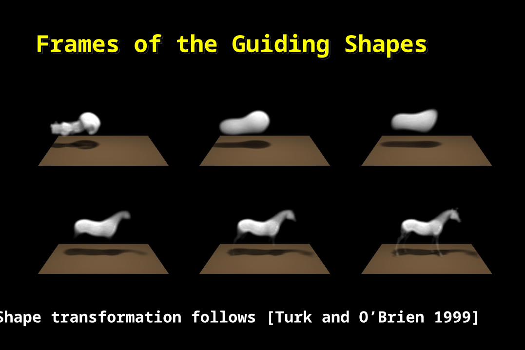
Frames of the Guiding ShapesFrames of the Guiding ShapesFrames of the Guiding ShapesFrames of the Guiding Shapes

Shape transformation follows [Turk and O’Brien 1999]

Corresponding Smoke AnimationCorresponding Smoke AnimationCorresponding Smoke AnimationCorresponding Smoke Animation

Basic Approach IIBasic Approach IIBasic Approach IIBasic Approach II

• Controlling smoke motion thus becomes a shape matching and tracking problem.– At each frame, measure the discrepancy between the

smoke region and the underlying guiding shape.– Error Metrics:

– Design a feedback force field on the smoke boundary to reduce the amount of discrepancy.

• Controlling smoke motion thus becomes a shape matching and tracking problem.– At each frame, measure the discrepancy between the

smoke region and the underlying guiding shape.– Error Metrics:

– Design a feedback force field on the smoke boundary to reduce the amount of discrepancy.

1 1

1/

( , )(1 ( , )) ( , )(1 ( , ))

( , )P

v i D i D i i

p

p

L

e t t d t t d

e D t d

x x x x x x

x x

Velocity ConstraintsVelocity ConstraintsVelocity ConstraintsVelocity Constraints

Velocity ConstraintsVelocity ConstraintsVelocity ConstraintsVelocity Constraints

n max( , ) min( ,| ( , ) |) msgn( , )

1, if ( , ) 0msgn( , )

sgn( ), otherwise

b i n b i b i

b ib i

t C d D t t

D tx t

D

u x x x

x

Normal component:

1L

1

i i

i it t

x x

u t ( , ) min( , )t tb i t

t

Ct

K

uu x u

u

Tangential component:

Revised Fluid SimulationRevised Fluid SimulationRevised Fluid SimulationRevised Fluid SimulationInvisid, incompressible Navier-Stokes equations:Invisid, incompressible Navier-Stokes equations:

t p u u u f 0 uThe iteration steps are [Fedkiw et al 2001]:• Compute intermediate velocity field u* ignoring the pressure term:

i) adding forces (gravity, external forces, etc)ii) perform semi-Lagrangian advection

• Detect the boundary of the smoke region using a density threshold;• Set up velocity constraints at the smoke boundary by modifying {u*}

• Projection:i) obtain pressure by solving the

Poisson equation,

ii) compute the velocity update via

2 * /p t u* t p u u

ResultsResultsResultsResults

Interaction with the EnvironmentInteraction with the EnvironmentInteraction with the EnvironmentInteraction with the Environment

Interaction between Smoke ObjectsInteraction between Smoke ObjectsInteraction between Smoke ObjectsInteraction between Smoke Objects

Smoke LettersSmoke LettersSmoke LettersSmoke Letters

Tradeoff between Shape Matching and Tradeoff between Shape Matching and Smoke AppearanceSmoke AppearanceTradeoff between Shape Matching and Tradeoff between Shape Matching and Smoke AppearanceSmoke Appearance

• Perfect shape matching makes the smoke does NOT look like smoke any more!

• Use thresholds on the error measures to control when the velocity constraints should be in effect.

• Perfect shape matching makes the smoke does NOT look like smoke any more!

• Use thresholds on the error measures to control when the velocity constraints should be in effect.

Related WorkRelated WorkRelated WorkRelated Work

• 1999, Stable Fluids, Stam• 1999, Shape Transformation Using Variational Implicit

Functions, Turk and O’Brien• 2001, Visual Simulation of Smoke, Fedkiw et al• 2002, Object Modeling and Animation with Smoke, Yu

and Shi• 2003, Keyframe Control of Smoke Simulations, Treuille et

al• 2004, Fluid Control Using the Adjoint Method, McNamara

et al• 2004, Target-Driven Smoke Animation, Fattal and

Lischinski

• 1999, Stable Fluids, Stam• 1999, Shape Transformation Using Variational Implicit

Functions, Turk and O’Brien• 2001, Visual Simulation of Smoke, Fedkiw et al• 2002, Object Modeling and Animation with Smoke, Yu

and Shi• 2003, Keyframe Control of Smoke Simulations, Treuille et

al• 2004, Fluid Control Using the Adjoint Method, McNamara

et al• 2004, Target-Driven Smoke Animation, Fattal and

Lischinski

Taming Liquids for Rapidly Taming Liquids for Rapidly Changing TargetsChanging TargetsTaming Liquids for Rapidly Taming Liquids for Rapidly Changing TargetsChanging Targets

Symposium on Computer Animation, 2005

In a NutshellIn a NutshellIn a NutshellIn a Nutshell

ObjectivesObjectivesObjectivesObjectives• Control capability

– Controlling liquids to match rapidly changing target shapes

• Ease to use• Fluid-like motion

– Should not overconstrain the fluid and preserve its natural movement as much as possible.

• Stability– The controlled movement should be stable without obvious

oscillations.

• Control capability– Controlling liquids to match rapidly changing target shapes

• Ease to use• Fluid-like motion

– Should not overconstrain the fluid and preserve its natural movement as much as possible.

• Stability– The controlled movement should be stable without obvious

oscillations.

System OverviewSystem OverviewSystem OverviewSystem Overview

,t t u t tu t t t tf

[Enright et al. 2002],T T

t t u

Feedback

Potential

Feedback Control ForcesFeedback Control ForcesFeedback Control ForcesFeedback Control Forces

feedback shape velocity f f f

Compensates for shape differences (proportional control)

Compensates for velocity differences (derivative control)

Velocity Feedback IVelocity Feedback IVelocity Feedback IVelocity Feedback I

velocity L T f x v v

Gain for derivative control

Velocity of the liquid at x

Target velocity at x

Velocity Feedback IIVelocity Feedback IIVelocity Feedback IIVelocity Feedback II

• Determine target velocity inside target object– Rigid body motion : compute from angular velocity

and velocity of center of mass– Articulated body : compute from the rigid body motion

of the segments it belongs to– Deformable surface : assume vertices are consistent

then extrapolate from surface velocity

• Determine target velocity outside target object– Velocity extrapolation [The fast construction of

extension velocities in level set methods, Adalsteinsson and Sethian, 1999]

• Determine target velocity inside target object– Rigid body motion : compute from angular velocity

and velocity of center of mass– Articulated body : compute from the rigid body motion

of the segments it belongs to– Deformable surface : assume vertices are consistent

then extrapolate from surface velocity

• Determine target velocity outside target object– Velocity extrapolation [The fast construction of

extension velocities in level set methods, Adalsteinsson and Sethian, 1999]

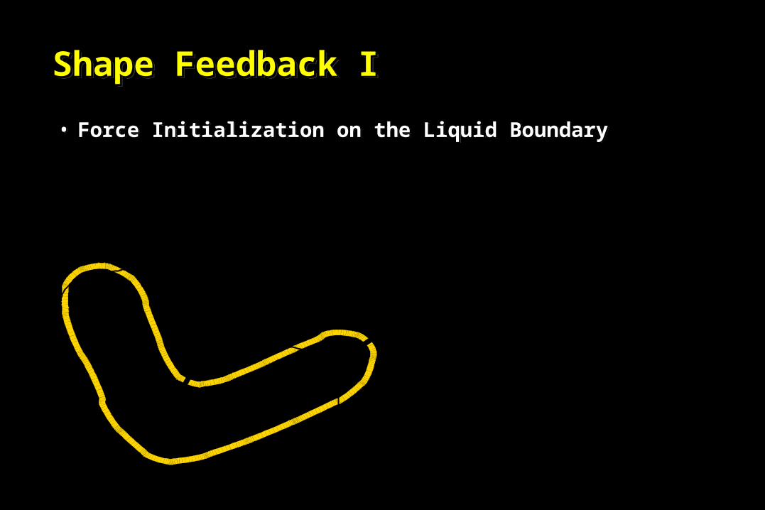
Shape Feedback IShape Feedback IShape Feedback IShape Feedback I

• Force Initialization on the Liquid Boundary• Force Initialization on the Liquid Boundary

1T

TT

dd

d

f x

2L

TL

dd

d

f x

Shape Feedback IIShape Feedback IIShape Feedback IIShape Feedback II

• Force Optimization on the Liquid Boundary [Computational methods for fluid flow, Peyret and Taylor, 1985]

• Force Optimization on the Liquid Boundary [Computational methods for fluid flow, Peyret and Taylor, 1985]

3

1

0j ji i i i

i i j

f n

f f n

, 1,...,i i i i mm

ff f n

Lagrangian Multiplier

Shape Feedback IIIShape Feedback IIIShape Feedback IIIShape Feedback III

2 0, H H

f

shape Hf

• The Complete Shape Feedback Force Field– Solving Laplace equation

• The Complete Shape Feedback Force Field– Solving Laplace equation

– Then

Geometric PotentialGeometric Potential [Hong and Kim 2004][Hong and Kim 2004]Geometric PotentialGeometric Potential [Hong and Kim 2004][Hong and Kim 2004]

Example IExample IExample IExample I

MOCAP data + skin Grid size 300x300x300 7 min per frameMOCAP data + skin Grid size 300x300x300 7 min per frame

Example IIExample IIExample IIExample II

Bouncing dumbbell Grid size 300x300x300 3.2 min per frameBouncing dumbbell Grid size 300x300x300 3.2 min per frame

Example IVExample IVExample IVExample IV

One dolphin Grid size 234x180x108 4.8 min per frameOne dolphin Grid size 234x180x108 4.8 min per frame

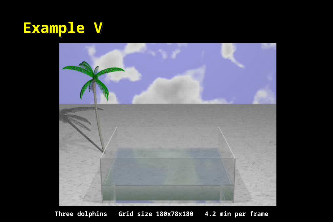
Example VExample VExample VExample V

Three dolphins Grid size 180x78x180 4.2 min per frame

Example VIExample VIExample VIExample VI

Water Horse Grid Size 275x250x75 4.4 min per frameWater Horse Grid Size 275x250x75 4.4 min per frame

Example VI MeshExample VI MeshExample VI MeshExample VI Mesh

Water Horse Grid Size 275x250x75 4.4 min per frameWater Horse Grid Size 275x250x75 4.4 min per frame

ConclusionsConclusionsConclusionsConclusions

• An overall framework for solving the fluid control problem

• An automatic scheme for matching a (rapidly changing) target shape based on the motion of the fluid

• Three tunable parameters to generate desired simulations

• Very efficient

• An overall framework for solving the fluid control problem

• An automatic scheme for matching a (rapidly changing) target shape based on the motion of the fluid

• Three tunable parameters to generate desired simulations

• Very efficient

Granular MaterialsGranular MaterialsGranular MaterialsGranular Materials

• Sand, soil, powders, and grains – Large collections of macroscopic particles

• Can resemble solids, liquids, and gases

• Also exhibit unique behaviors

• Sand, soil, powders, and grains – Large collections of macroscopic particles

• Can resemble solids, liquids, and gases

• Also exhibit unique behaviors

Granular PhenomenaGranular PhenomenaGranular PhenomenaGranular Phenomena

• Angle of Repose• Angle of Repose

Fluidized surface layer Stagnant Interior

Solid-like behavior

Granular PhenomenaGranular PhenomenaGranular PhenomenaGranular Phenomena

• Silos and Hourglasses• Silos and Hourglasses

height dependent height independent Constant flow rate

Fluid

Granular

Granular PhenomenaGranular PhenomenaGranular PhenomenaGranular Phenomena

• Force Chains– Highly stressed particles

– Discrete nature

• Force Chains– Highly stressed particles

– Discrete nature

Related Work in GraphicsRelated Work in GraphicsRelated Work in GraphicsRelated Work in Graphics

• Empirical models– Interactive rates– Sumner et al. [1999]

• Discrete models– Particles modeled explicitly– Reproduce granular phenomena– Luciani et al. [1995]

• Continuum models– Only viable method for some systems– Less physically accurate than discrete– Zhu and Bridson [2005]

• Empirical models– Interactive rates– Sumner et al. [1999]

• Discrete models– Particles modeled explicitly– Reproduce granular phenomena– Luciani et al. [1995]

• Continuum models– Only viable method for some systems– Less physically accurate than discrete– Zhu and Bridson [2005]

GoalsGoalsGoalsGoals

• Accurate reproduction of granular phenomena• Two-way coupling with rigid objects• Large-scale systems ( >100K particles )• Ease of implementation

• Accurate reproduction of granular phenomena• Two-way coupling with rigid objects• Large-scale systems ( >100K particles )• Ease of implementation

Discrete ModelsDiscrete ModelsDiscrete ModelsDiscrete Models

• Event Driven Method– No overlapping– Instantaneous change in momentum– Appropriate for sparse systems with long intervals between

consecutive collisions

• Molecular Dynamics Method– Some overlap permitted– Forces determined by overlap– No distinction between collision and contact– Efficient handling of persistent and transient contact

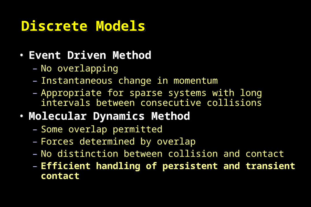
• Event Driven Method– No overlapping– Instantaneous change in momentum– Appropriate for sparse systems with long intervals between

consecutive collisions

• Molecular Dynamics Method– Some overlap permitted– Forces determined by overlap– No distinction between collision and contact– Efficient handling of persistent and transient contact

Contact ForcesContact ForcesContact ForcesContact Forces

• Normal Force– A Restorative force to resist overlap– A Dissipative force for damping

• Tangential Force– A Shear force for friction

• Normal Force– A Restorative force to resist overlap– A Dissipative force for damping

• Tangential Force– A Shear force for friction

Normal ForceNormal ForceNormal ForceNormal Force

• Damped Linear Spring– Sufficient for many applications

• More accurate alternatives

• Damped Linear Spring– Sufficient for many applications

• More accurate alternatives

Normal force

Dissipation Coefficient Restoration Coefficient

OverlapRelative velocity

Normal ForceNormal ForceNormal ForceNormal Force

• Hertz Contact– Relates restoration coefficient to material properties

• Young’s Modulus & Poisson Ratio

• Implicitly handles particle size scaling

• Hertz Contact– Relates restoration coefficient to material properties

• Young’s Modulus & Poisson Ratio

• Implicitly handles particle size scaling

Normal force

OverlapRelative velocity

Restoration CoefficientDissipation Coefficient

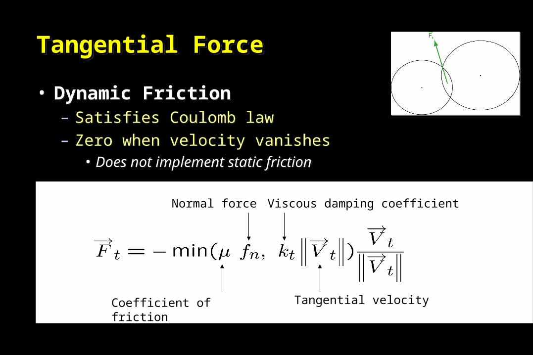
Tangential ForceTangential ForceTangential ForceTangential Force

• Dynamic Friction– Satisfies Coulomb law– Zero when velocity vanishes

• Does not implement static friction

• Dynamic Friction– Satisfies Coulomb law– Zero when velocity vanishes

• Does not implement static friction

Coefficient of friction

Normal force Viscous damping coefficient

Tangential velocity

Static FrictionStatic FrictionStatic FrictionStatic Friction

• Use geometric roughness for static friction– Non-spherical granular particles formed from rigidly

bonded spheres– Constrained to move as a single rigid body

• Use geometric roughness for static friction– Non-spherical granular particles formed from rigidly

bonded spheres– Constrained to move as a single rigid body

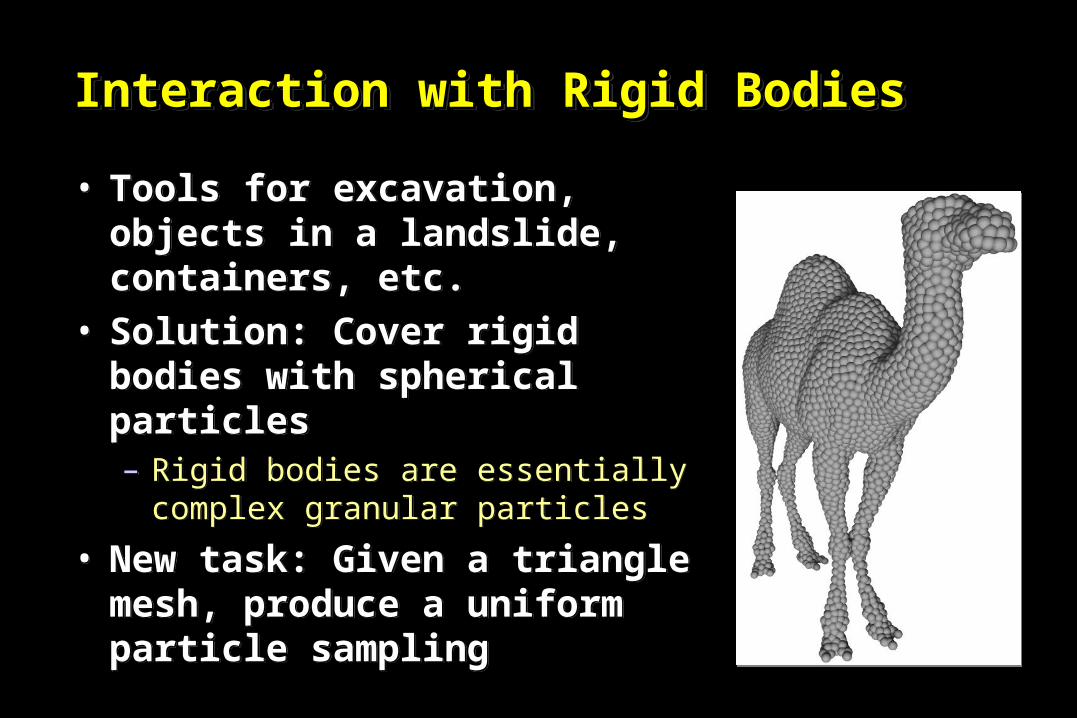
Interaction with Rigid BodiesInteraction with Rigid BodiesInteraction with Rigid BodiesInteraction with Rigid Bodies

• Tools for excavation, objects in a landslide, containers, etc.

• Solution: Cover rigid bodies with spherical particles– Rigid bodies are essentially complex

granular particles

• New task: Given a triangle mesh, produce a uniform particle sampling

• Tools for excavation, objects in a landslide, containers, etc.

• Solution: Cover rigid bodies with spherical particles– Rigid bodies are essentially complex

granular particles

• New task: Given a triangle mesh, produce a uniform particle sampling

Interaction with Rigid BodiesInteraction with Rigid BodiesInteraction with Rigid BodiesInteraction with Rigid Bodies

• Convert mesh to implicit representation – Signed distance transform

• Sample implicit with particles – [Witkin & Heckbert 1994]– Particles “float” along surface– Simple repulsion model produces uniform sampling

• Convert mesh to implicit representation – Signed distance transform

• Sample implicit with particles – [Witkin & Heckbert 1994]– Particles “float” along surface– Simple repulsion model produces uniform sampling

Collision DetectionCollision DetectionCollision DetectionCollision Detection

• Reduces to finding overlapping spheres

• Assuming all spheres are of similar size…– Use spatial hashing with

voxel size equal to diameter of largest sphere

• Reduces to finding overlapping spheres

• Assuming all spheres are of similar size…– Use spatial hashing with

voxel size equal to diameter of largest sphere

Video

AcknowledgmentsAcknowledgmentsAcknowledgmentsAcknowledgments

• Lin Shi, Nathan Bell, Peter Mucha, Stephen Bond

• NSF

• UIUC Research Board

• Lin Shi, Nathan Bell, Peter Mucha, Stephen Bond

• NSF

• UIUC Research Board

Thank You!Thank You!Thank You!Thank You!

In each time step…In each time step…In each time step…In each time step…

• Compute intermediate velocity field {u*};• Detect the boundary of the smoke region using a

density threshold;• Set up velocity constraints at the smoke boundary

by modifying {u*}• Solve the final fluid velocity field while satisfying

the velocity constraints• Evolve the smoke density

• Compute intermediate velocity field {u*};• Detect the boundary of the smoke region using a

density threshold;• Set up velocity constraints at the smoke boundary

by modifying {u*}• Solve the final fluid velocity field while satisfying

the velocity constraints• Evolve the smoke density

Empirical Equation for Compressible GasesEmpirical Equation for Compressible GasesEmpirical Equation for Compressible GasesEmpirical Equation for Compressible Gases

( ) ( )t u u u u f

Empirical Equation:

New Projection Step:

• Obtain the pressure by solving

• Apply a diffusion process

• Update velocity

2 * /p t u

2P PP

t

2 2( )t P u u

Comparison between Incompressible and Comparison between Incompressible and Compressible Fluid ModelsCompressible Fluid ModelsComparison between Incompressible and Comparison between Incompressible and Compressible Fluid ModelsCompressible Fluid Models

Incompressible Compressible

Effects of Error ThresholdsEffects of Error ThresholdsEffects of Error ThresholdsEffects of Error Thresholds

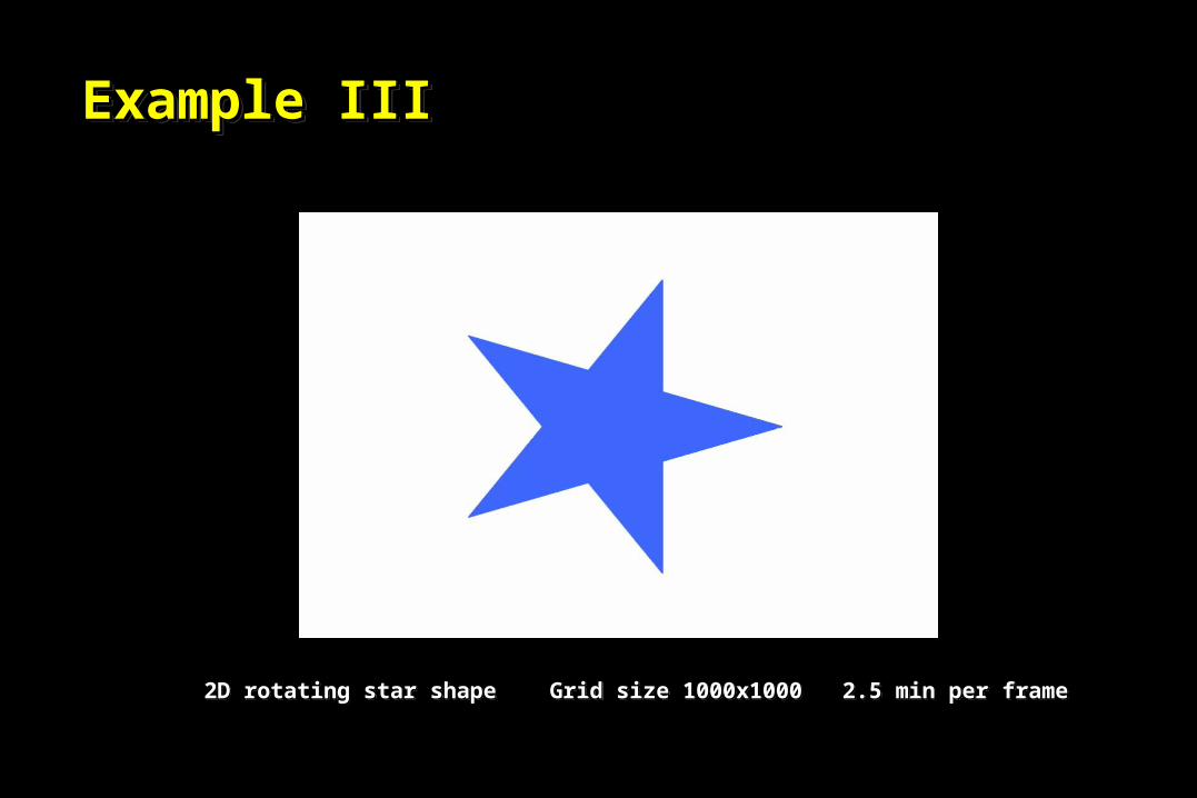
Example IIIExample IIIExample IIIExample III

2D rotating star shape Grid size 1000x1000 2.5 min per frame2D rotating star shape Grid size 1000x1000 2.5 min per frame

Surface Flow SimulationSurface Flow SimulationSurface Flow SimulationSurface Flow Simulation

Surface Flow Simulation IISurface Flow Simulation IISurface Flow Simulation IISurface Flow Simulation II

Time IntegrationTime IntegrationTime IntegrationTime Integration

• Granular Particles and Rigid Objects follow rigid body dynamics

• Corresponding ODEs solved with adaptive Runge-Kutta method– Adaptive since required time step varies greatly

• Granular Particles and Rigid Objects follow rigid body dynamics

• Corresponding ODEs solved with adaptive Runge-Kutta method– Adaptive since required time step varies greatly