© 2017 IOP Publishing Ltd

1. Introduction

Flying snakes have evolved a form of aerial locomotion unique among flyers. Because the snakes lack any specialized flight anatomy, they have to use their entire body to produce aerodynamic forces both to oppose gravity and to control the trajectory. Upon becoming airborne, the snakes splay their ribs laterally and create a ‘wing’ with an unconventional cross-sectional shape. Simultaneously, they assume an S-like shape and send high-amplitude traveling waves posteriorly down the body, producing aerial undulation (Socha 2002, 2006, 2011, Socha and LaBarbera 2005, Socha et al 2005, 2010, 2015). Compared to other biological or engineered flyers that use paired, bilaterally symmetric wings (Alexander 2003, Biewener 2003), gliding in

snakes exhibits a number of unique characteristics. In particular, (i) snakes glide with a highly dynamic behavior in the form of undulation, as opposed to the generally static posture of other gliders; (ii) the snake’s body posture is not bilaterally symmetrical at any moment in time; and (iii) undulatory motion involves significant out-of-plane translation of different parts of the body.

Because the dynamic effects of aerial undula-tion are manifested by the continuous redistribution of body mass and aerodynamic forces, undulation should play some functional role related to the snake’s aerial performance, stability, or control. However, despite the growing number of studies on the physi-cal basis of gliding in snakes, the question of the func-tional role of undulation has not been answered. Jafari

F Jafari et al

066002

BBIICI

© 2017 IOP Publishing Ltd

12

Bioinspir. Biomim.

BB

1748-3190

10.1088/1748-3190/aa8c2f

6

1

14

Bioinspiration & Biomimetics

IOP

6

October

2017

Control of gliding in a flying snake-inspired n-chain model

Farid Jafari , Sevak Tahmasian, Shane D Ross and John J SochaDepartment of Biomedical Engineering and Mechanics, Virginia Tech, Blacksburg, VA, United States of America

E-mail: jafari@vt.edu (F Jafari)

Keywords: flying snakes, gliding, stability, dynamical model, vibrational control

Supplementary material for this article is available online

AbstractFlying snakes of genus Chrysopelea possess a highly dynamic gliding behavior, which is dominated by an undulation in the form of lateral waves sent posteriorly down the body. The resulting high-amplitude periodic variations in the distribution of mass and aerodynamic forces have been hypothesized to contribute to the stability of the snake’s gliding trajectory. However, a previous 2D analysis in the longitudinal plane failed to reveal a significant effect of undulation on the stability in the pitch direction. In this study, a theoretical model was used to examine the dynamics and stability characteristics of flying snakes in three dimensions. The snake was modeled as an articulated chain of airfoils connected with revolute joints. Along the lines of vibrational control methods, which employ high-amplitude periodic inputs to produce desirable stable motions in nonlinear systems, undulation was considered as a periodic input to the system. This was implemented either by directly prescribing the joint angles as periodic functions of time (kinematic undulation), or by assuming periodic torques acting at the joints (torque undulation). The aerodynamic forces were modeled using blade element theory and previously determined force coefficients. The results show that torque undulation, along with linearization-based closed-loop control, could increase the size of the basin of stability. The effectiveness of the stabilization provided by torque undulation is a function of the amplitude and frequency of the input. In addition, kinematic undulation provides open-loop stability for sufficiently large frequencies. The results suggest that the snakes need some amount of closed-loop control despite the clear contribution of undulation to glide stability. However, as the closed-loop control system needs to work around a passively stable trajectory, undulation lowers the demand for a complex closed-loop control system. Overall, this study demonstrates the possibility of maintaining stability during gliding using a morphing body instead of symmetrically paired wings.

PAPER2017

RECEIVED 11 February 2017

REVISED

4 September 2017

ACCEPTED FOR PUBLICATION

13 September 2017

PUBLISHED 6 October 2017

https://doi.org/10.1088/1748-3190/aa8c2fBioinspir. Biomim. 12 (2017) 066002

2

F Jafari et al

et al (2014) developed 2D theoretical models of flying snakes to test the hypothesis that undulation contrib-utes to stability in the pitch direction. They concluded that undulation has a limited capacity for providing longitudinal stability. Socha and LaBarbera (2005) used experimental kinematics data to show that vari-ations in undulation were only weakly correlated to glide performance. In particular, they found no rela-tion between performance and undulation frequency, which suggests that frequency is not involved in aero-dynamic force production. As a corollary, this also suggests that the quasi-steady forces produced by the animal’s forward speed are sufficient to enable glid-ing. Holden et al (2014) made the same argument based on the large advance ratios observed in flying snakes. These studies suggest that undulation is not particularly important, yet this motion is the aerial snake’s most prominent behavior.

With our current understanding of the mechan-ics of gliding in snakes, the strongest hypothesis about the function of undulation concerns stability. This hypothesis may seem to contradict the aforemen-tioned results of Jafari et al (2014), that undulation has limited capacity to provide stability. However, Jafari et al (2014) analyzed only the longitudinal dynamics of the snakes, and only the effects of undulation in the pitch direction were considered. Undulation could still influence pitch through 3D effects not considered in Jafari et al (2014), and it is also possible that undula-tion contributes to stability in the roll and yaw direc-tions. The possibility of such stability is suggested by the following line of reasoning. In the S-shaped pos-ture, the snake is bilaterally asymmetric at any moment of time. This asymmetry, even in the absence of distur-bances, produces unfavorable non-zero moments that drive the snake’s body to rotate, potentially causing it to spin out of control. However, the average body pos-ture over one undulation cycle is symmetric, and the symmetric averaged posture could cause the moments about the fore-aft axis to periodically vary about zero means. Under certain conditions that depend on the relative timescales of the motions, zero-mean periodic moments would cause the snake to wobble about the upright position without losing control, where the ‘upright position’ refers to the observed body orienta-tion in gliding, in which the dorsal surface of the body faces upward.

The methods of vibrational control lend insight in how to produce desirable changes in the dynamic response and properties of nonlinear mechanical systems using high-frequency, zero-mean periodic inputs (Meerkov 1980). Applying periodic inputs in a mechanical system may change the stability properties, natural frequencies, transient response, and equilib-ria of the system (Thomsen 2005). The simplest and most well-known example is the Stephenson–Kapitza pendulum (Kapitza 1951), a simple inverted pendu-lum with a pivot free to move along the vertical line. By vibrating the pivot vertically with sufficiently high fre-

quency, the unstable upward position of the pendulum can be stabilized without using feedback control. Thus, it is theoretically possible for flying snakes to exploit properties of periodic motions, suggesting that vibra-tional control theory may prove useful for analysis.

Employing periodic inputs to control mechanical systems generally gives rise to periodic steady-state motions that are not easy to find and characterize. Nev-ertheless, for a large class of time-periodic mechanical systems, the averaging theorem provides a powerful tool to predict the existence and determine the stabil-ity of periodic solutions (Bullo 2002, Guckenheimer and Holmes 2013). Physically speaking, when the inputs oscillate much more rapidly than the natural dynamics of the system, the state of the system can be approximated to remain the same during one input cycle. The averaging theorem averages the dynamics over one input cycle and introduces a time-invariant (or autonomous) system that approximately has the same trajectory and stability characteristics as the original time-periodic system. In vibrational control, the approach is usually to use the averaging theorem to replace the original time-periodic dynamics with the averaged time-invariant system. Next, the averaged system is designed to possess a desirable stable equilib-rium solution, about which the time-periodic system is ensured to have a stable periodic orbit. The required inputs are then found according to the aforemen-tioned design. With this technique, the control is open loop, and the desired motion is achieved without any feedback from the state of the system. It is imperative to note that the necessary condition for the averaging theorem to be valid is that the frequency of inputs must be larger than a certain value, which depends on the physical parameters of the system. However, the mini-mum required frequency cannot be determined from the averaging theorem itself. In practice, a trial-and-error approach is usually used to select the input fre-quency that makes the stabilization work (Tahmasian and Woolsey 2015). Averaging techniques have found widespread applications in stabilization and control of biomimetic systems incluing robotic fish (Morgansen et al 2002), flapping wing micro-air vehicles (Tahma-sian et al 2014), and snake robots (Liljebäck et al 2010). Averaging techniques have also been used to ana-lyze the dynamics of biological systems such as flying insects (Taha et al 2015).

In this work, we treat flying snakes as nonlinear mechanical systems, with undulation as a zero-mean periodic input. According to vibrational control the-ory, it might be possible that a snake undulates to take advantage of the properties of periodic motions and obtain some degree of passive stability. We examine this hypothesis using a theoretical approach by repre-senting the snake as a chain of successively linked air-foils and developing a dynamical framework for its 3D motions. Within this framework, the snake’s postural reconfigurations can be approximated by changing the orientations of the airfoils. Using joint torques as

Bioinspir. Biomim. 12 (2017) 066002

3

F Jafari et al

the control inputs, the complexity of the model can be adjusted to the control requirements. Specifically, we examine the influence of changing the number of links, as well as the amplitude and frequency of the periodic inputs, on the stability characteristics of the model. In this regard, we determine the minimum number of links and the minimum frequency neces-sary to stabilize the model. Using this model, we test the hypothesis that flying snakes undulate to maintain their flight stability.

2. Methods

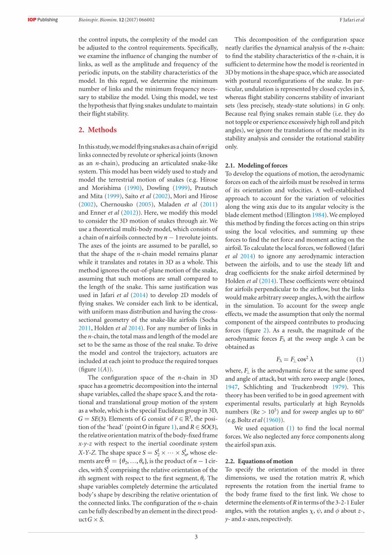
In this study, we model flying snakes as a chain of n rigid links connected by revolute or spherical joints (known as an n-chain), producing an articulated snake-like system. This model has been widely used to study and model the terrestrial motion of snakes (e.g. Hirose and Morishima (1990), Dowling (1999), Prautsch and Mita (1999), Saito et al (2002), Mori and Hirose (2002), Chernousko (2005), Maladen et al (2011) and Enner et al (2012)). Here, we modify this model to consider the 3D motion of snakes through air. We use a theoretical multi-body model, which consists of a chain of n airfoils connected by −n 1 revolute joints. The axes of the joints are assumed to be parallel, so that the shape of the n-chain model remains planar while it translates and rotates in 3D as a whole. This method ignores the out-of-plane motion of the snake, assuming that such motions are small compared to the length of the snake. This same justification was used in Jafari et al (2014) to develop 2D models of flying snakes. We consider each link to be identical, with uniform mass distribution and having the cross-sectional geometry of the snake-like airfoils (Socha 2011, Holden et al 2014). For any number of links in the n-chain, the total mass and length of the model are set to be the same as those of the real snake. To drive the model and control the trajectory, actuators are included at each joint to produce the required torques (figure 1(A)).

The configuration space of the n-chain in 3D space has a geometric decomposition into the internal shape variables, called the shape space S, and the rota-tional and translational group motion of the system as a whole, which is the special Euclidean group in 3D,

( )=G SE 3 . Elements of G consist of → R∈r 3, the posi-tion of the ‘head’ (point O in figure 1), and ( )∈R SO 3 , the relative orientation matrix of the body-fixed frame x-y-z with respect to the inertial coordinate system

X-Y-Z. The shape space = × ×S S Sn21 1, whose ele-

ments are →

θ θΘ = …, , n2 , is the product of −n 1 cir-

cles, with Si1 comprising the relative orientation of the

ith segment with respect to the first segment, θi. The shape variables completely determine the articulated body’s shape by describing the relative orientation of the connected links. The configuration of the n-chain can be fully described by an element in the direct prod-uct ×G S.

This decomposition of the configuration space neatly clarifies the dynamical analysis of the n-chain: to find the stability characteristics of the n-chain, it is sufficient to determine how the model is reoriented in 3D by motions in the shape space, which are associated with postural reconfigurations of the snake. In par-ticular, undulation is represented by closed cycles in S, whereas flight stability concerns stability of invariant sets (less precisely, steady-state solutions) in G only. Because real flying snakes remain stable (i.e. they do not topple or experience excessively high roll and pitch angles), we ignore the translations of the model in its stability analysis and consider the rotational stability only.

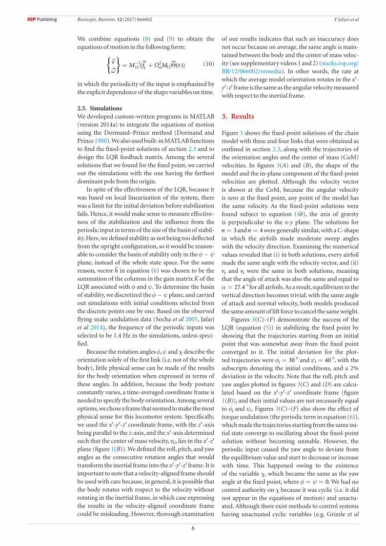
2.1. Modeling of forcesTo develop the equations of motion, the aerodynamic forces on each of the airfoils must be resolved in terms of its orientation and velocities. A well-established approach to account for the variation of velocities along the wing axis due to its angular velocity is the blade element method (Ellington 1984). We employed this method by finding the forces acting on thin strips using the local velocities, and summing up these forces to find the net force and moment acting on the airfoil. To calculate the local forces, we followed (Jafari et al 2014) to ignore any aerodynamic interaction between the airfoils, and to use the steady lift and drag coefficients for the snake airfoil determined by Holden et al (2014). These coefficients were obtained for airfoils perpendicular to the airflow, but the links would make arbitrary sweep angles, λ, with the airflow in the simulation. To account for the sweep angle effects, we made the assumption that only the normal component of the airspeed contributes to producing forces (figure 2). As a result, the magnitude of the aerodynamic forces λF at the sweep angle λ can be obtained as

λ=λ ⊥F F cos2 (1)

where, ⊥F is the aerodynamic force at the same speed and angle of attack, but with zero sweep angle (Jones, 1947, Schlichting and Truckenbrodt 1979). This theory has been verified to be in good agreement with experimental results, particularly at high Reynolds numbers (Re > 105) and for sweep angles up to 60° (e.g. Boltz et al (1960)).

We used equation (1) to find the local normal forces. We also neglected any force components along the airfoil span axis.

2.2. Equations of motionTo specify the orientation of the model in three dimensions, we used the rotation matrix R, which represents the rotation from the inertial frame to the body frame fixed to the first link. We chose to determine the elements of R in terms of the 3-2-1 Euler angles, with the rotation angles χ, ψ, and φ about z-, y- and x-axes, respectively.

Bioinspir. Biomim. 12 (2017) 066002

4

F Jafari et al

To explicitly write the equations of motion for an arbitrary number of links, we selected the veloci-ties expressed in the body-fixed frame x-y-z (com-monly called the quasi-velocities) as the variables, and summed the Newton–Euler equations over all of the segments to obtain the dynamic equations in G. The dynamic equations in S were derived by writing the moment equation about each joint axis. This approach was identical to using Kane’s method (Kane and Lev-inson 1985). The equations of motion were compiled in the following compact form:

⎪ ⎪

⎪ ⎪

⎧⎨⎪

⎩⎪

⎫⎬⎪

⎭⎪

⎧⎨⎩

⎫⎬⎭

ω φ ψ ωτ

Θ

Θ

= Θ Θ +M

v

f v0000, , , , ,

..

( )˙˙ ( ˙ ) (2)

where →v is the velocity of the ‘head’, and →ω is the angular velocity of the body-fixed frame, both expressed in the x-y-z coordinates. Matrix M contains the inertial terms and is a function of shape variables only, and →f is the drift vector resulting from the gravitational, aerodynamic, and second-degree velocity terms. Also, →τ represents the input torques exerted at the joints.

To obtain a complete set of equations describing the motion, the dynamical equations were supple-mented by the following kinematic relation:

⎧⎨⎪

⎩⎪

⎫⎬⎪

⎭⎪

φψχ

φ ψ ω=t

Jd

d,( ) (3)

where J is the Jacobian of the rotation matrix (Baruh 1999).

2.3. Controlled motion about a fixed pointStandard methods to calculate stability in a multi-dimensional state space require obtaining an invariant set, whose stability can be determined linearly. We started analyzing the n-chain model with the simplest invariant set, a fixed point. Because neither the position vector →r nor the rotation angle χ appears in equations (2) and (3), these variables were omitted from the state vector. Moreover, because our focus was on the roll and pitch motions, which are not influenced by the angle χ, we did not attempt to control this angle. Nonetheless, it should be noted that it is possible to control χ by a cascading controller through χ. Therefore, a fixed point was determined using

⎧

⎨⎪

⎩⎪

ωφ ψ= == =

Θ = Θ =

v 00

00

0 ...

˙ ˙˙ ˙

˙ (4a)

To ensure an upright configuration of the chain model, equation (4a) was augmented with the following conditions:

φ ψ= =0, 0e e (4b)

where the subscripts indicate equilibrium values.To control the roll and pitch angles, the model

requires at least two inputs, which must be supplied by the joint torques. Therefore, the simplest chain had to incorporate three links. After substituting equa-tions (4a) and (4b) into (2) and (3), we solved for →ve, →ωe,

→Θe, and →τe, in which the subscript denotes the values

at the fixed point solution, →xe. Next, we linearized the

Figure 1. Overview of the n-chain model. (A) A representative view of the n-chain model with n = 3 identical links. The inset shows the snake-like cross-sectional shape of the links. The x-y-z frame is fixed to the first link, whereas the X-Y-Z coordinate system is inertial. The entire body of the model, which is viewed from the z-direction in this figure, lies in the x-y plane. The shape of the model is determined by the angle each link makes with the x-axis. The overall position and orientation of the model are determined by the position vector →r and the orientation of x-y-z frame relative to the X-Y-Z frame. The joint torques represent the effort needed to change the shape of the n-chain. (B) The roll, pitch, and yaw angles are defined based on the x′-y′-z′ coordinate frame, in which the z′-axis is parallel to the z-axis, and the x′-axis is determined such that the center of mass velocity, vG, lies in the x′-z′ plane.

Bioinspir. Biomim. 12 (2017) 066002

5

F Jafari et al

nonlinear equations of motion about the fixed point to obtain the local state-space time-invariant form. We then used the linear quadratic regulator (LQR), a well-known feedback control scheme, to stabilize the fixed point solution (Sontag 1998). As a result, the joint tor-ques were determined as:

( )→ → → →τ τ= − −K x xe e (5)

with →x being the system state, and K some constant gain matrix determined by the LQR. Although the stabilization rendered by equation (5) was obtained for the locally linearized system, it tended to work within a fair neighborhood of the fixed point due to the robustness of the LQR.

This procedure was repeated for a 4-link model. The extra degree of freedom made it possible to control the yaw rate, χ, in addition to the conditions expressed in equations (4a) and (4b). To this end, we replaced the second line of equation (4a) with →ω =00.

To examine whether adding periodicity to the input (vibrational control) can enhance the stabilizing properties of the designed feedback control, we revised equation (5) to incorporate a periodic term as

( )→ → → → →τ τ α= − − + ΩK x x h tsine e u u (6)

where Ωu is the input frequency, →h is a constant vector,

and αu is a scalar parameter determining the amplitude of input vibrations. As equation (6) prescribes oscillations in the input torque, the ensuing control scheme is called ‘torque undulation’ hereafter.

The procedure described above can likewise be used to control other motions such as yaw and sideslip,

as long as the number of input torques in the n-chain is equal or greater than the number of coordinates that are desired to be controlled.

2.4. Motion with shape undulationTo reproduce shape changes in the n-chain that resemble undulatory waves, we employed a sinusoidal wave of varying θis traveling posteriorly, with the entire model comprising one wavelength. Such a wave is written as:

( )⎛⎝⎜

⎞⎠⎟θ

ππ= −Ω = …t

j

nt j n

2cos 2 , 2, , .j u (7)

By differentiating equation (7) and substituting the results into equation (2), the rate of translation and rotation of the model, as well as the joint torques, could be determined. However, at this point, we were mostly interested in the passive stability that undulation could provide, without considering the required control effort. Therefore, to eliminate the torques from the calculations, we rewrote the whole-body equations of motion as:

⎪ ⎪

⎪ ⎪⎧⎨⎩

⎫⎬⎭ω= − ΘM v f M11 1 12

..→→

→ → (8)

in which M11, M12, and →f1 are proper partitions of

M and →f , and

→Θ..

takes the role of control inputs. It is

also evident from equation (7) that

Θ = −Ω Θu..

2 (9)

Figure 2. Modeling of the aerodynamic forces. The local forces in the blade element method were calculated using the local velocities and the steady lift and drag coefficients for the snake airfoil (A), as determined by Holden et al (2014) (reproduced with permission from (Holden et al 2014)). (B) Sweep angle, λ, was accounted for by using simple sweep theory, in which only the normal component of the velocity, ⊥v , contributes to force production (left). Any force component along the airfoil span axis is neglected (right).

Bioinspir. Biomim. 12 (2017) 066002

6

F Jafari et al

We combine equations (8) and (9) to obtain the equations of motion in the following form:

⎧

⎨⎩

⎫⎬⎭ω= +Ω Θ−v M f M tu11

11

212

˙˙ ( ( )) (10)

in which the periodicity of the input is emphasized by the explicit dependence of the shape variables on time.

2.5. SimulationsWe developed custom-written programs in MATLAB (version 2014a) to integrate the equations of motion using the Dormand–Prince method (Dormand and Prince 1980). We also used built-in MATLAB functions to find the fixed-point solutions of section 2.3 and to design the LQR feedback matrix. Among the several solutions that we found for the fixed point, we carried out the simulations with the one having the farthest dominant pole from the origin.

In spite of the effectiveness of the LQR, because it was based on local linearization of the system, there was a limit for the initial deviation before stabilization fails. Hence, it would make sense to measure effective-ness of the stabilization and the influence from the periodic input in terms of the size of the basin of stabil-ity. Here, we defined stability as not being too deflected from the upright configuration, so it would be reason-able to consider the basin of stability only in the φ ψ− plane, instead of the whole state space. For the same reason, vector

→h in equation (6) was chosen to be the

summation of the columns in the gain matrix K of the LQR associated with φ and ψ. To determine the basin of stability, we discretized the φ ψ− plane, and carried out simulations with initial conditions selected from the discrete points one by one. Based on the observed flying snake undulation data (Socha et al 2005, Jafari et al 2014), the frequency of the periodic inputs was selected to be 1.4 Hz in the simulations, unless speci-fied.

Because the rotation angles φ, ψ and χ describe the orientation solely of the first link (i.e. not of the whole body), little physical sense can be made of the results for the body orientation when expressed in terms of these angles. In addition, because the body posture constantly varies, a time-averaged coordinate frame is needed to specify the body orientation. Among several options, we chose a frame that seemed to make the most physical sense for this locomotor system. Specifically, we used the x′-y′-z′ coordinate frame, with the z′-axis being parallel to the z-axis, and the x′-axis determined such that the center of mass velocity, vG, lies in the x′-z′ plane (figure 1(B)). We defined the roll, pitch, and yaw angles as the consecutive rotation angles that would transform the inertial frame into the x′-y′-z′ frame. It is important to note that a velocity-aligned frame should be used with care because, in general, it is possible that the body rotates with respect to the velocity without rotating in the inertial frame, in which case expressing the results in the velocity-aligned coordinate frame could be misleading. However, thorough examination

of our results indicates that such an inacc uracy does not occur because on average, the same angle is main-tained between the body and the center of mass veloc-ity (see supplementary videos 1 and 2) (stacks.iop.org/BB/12/066002/mmedia). In other words, the rate at which the average model orientation rotates in the x′-y′-z′ frame is the same as the angular velocity measured with respect to the inertial frame.

3. Results

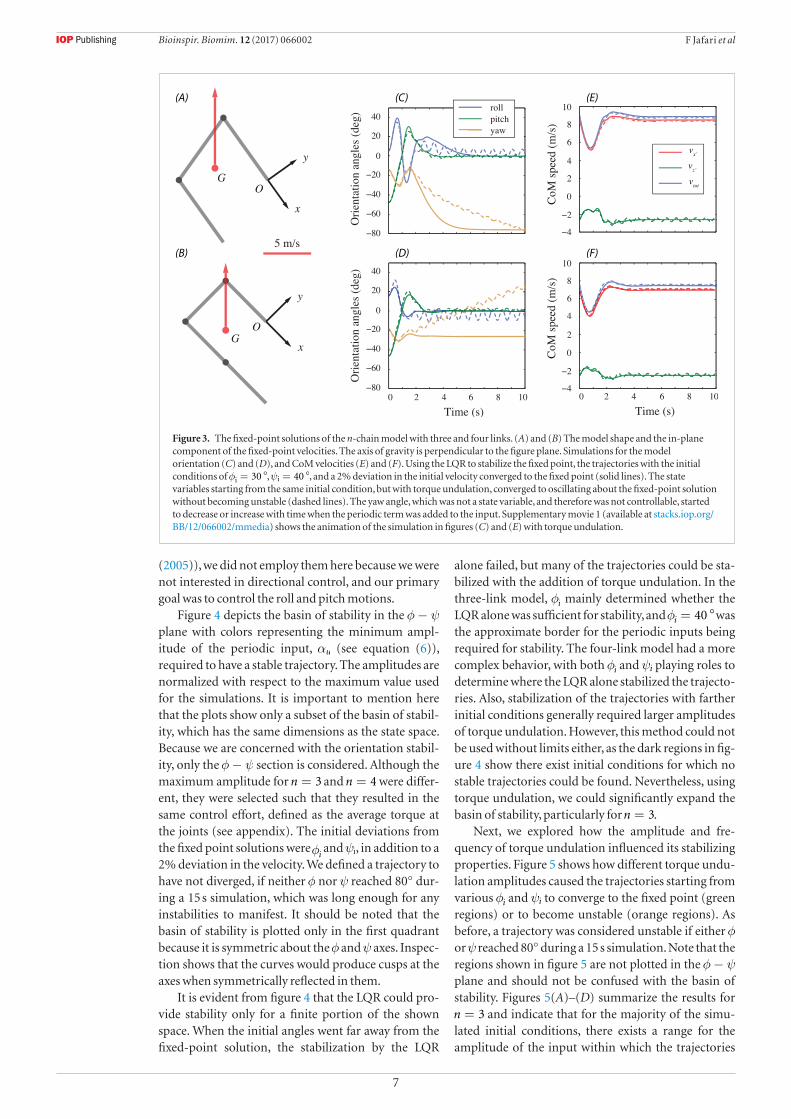
Figure 3 shows the fixed-point solutions of the chain model with three and four links that were obtained as outlined in section 2.3, along with the trajectories of the orientation angles and the center of mass (CoM) velocities. In figures 3(A) and (B), the shape of the model and the in-plane component of the fixed-point velocities are plotted. Although the velocity vector is shown at the CoM, because the angular velocity is zero at the fixed point, any point of the model has the same velocity. As the fixed-point solutions were found subject to equation (4b), the axis of gravity is perpendicular to the x-y plane. The solutions for =n 3 and =n 4 were generally similar, with a C-shape

in which the airfoils made moderate sweep angles with the velocity direction. Examining the numerical values revealed that (i) in both solutions, every airfoil made the same angle with the velocity vector, and (ii) vy and vz were the same in both solutions, meaning that the angle of attack was also the same and equal to α = °27.4 for all airfoils. As a result, equilibrium in the vertical direction becomes trivial; with the same angle of attack and normal velocity, both models produced the same amount of lift force to cancel the same weight.

Figures 3(C)–(F) demonstrate the success of the LQR (equation (5)) in stabilizing the fixed point by showing that the trajectories starting from an initial point that was somewhat away from the fixed point converged to it. The initial deviation for the plot-ted trajectories were φ = °30i and ψ = °40i , with the subscripts denoting the initial conditions, and a 2% deviation in the velocity. Note that the roll, pitch and yaw angles plotted in figures 3(C) and (D) are calcu-lated based on the x′-y′-z′ coordinate frame (figure 1(B)), and their initial values are not necessarily equal to φi and ψi. Figures 3(C)–(F) also show the effect of torque undulation (the periodic term in equation (6)), which made the trajectories starting from the same ini-tial state converge to oscillating about the fixed-point solution without becoming unstable. However, the periodic input caused the yaw angle to deviate from the equilibrium value and start to decrease or increase with time. This happened owing to the existence of the variable χ, which became the same as the yaw angle at the fixed point, where φ ψ= = 0. We had no control authority on χ because it was cyclic (i.e. it did not appear in the equations of motion) and unactu-ated. Although there exist methods to control systems having unactuated cyclic variables (e.g. Grizzle et al

Bioinspir. Biomim. 12 (2017) 066002

7

F Jafari et al

(2005)), we did not employ them here because we were not interested in directional control, and our primary goal was to control the roll and pitch motions.

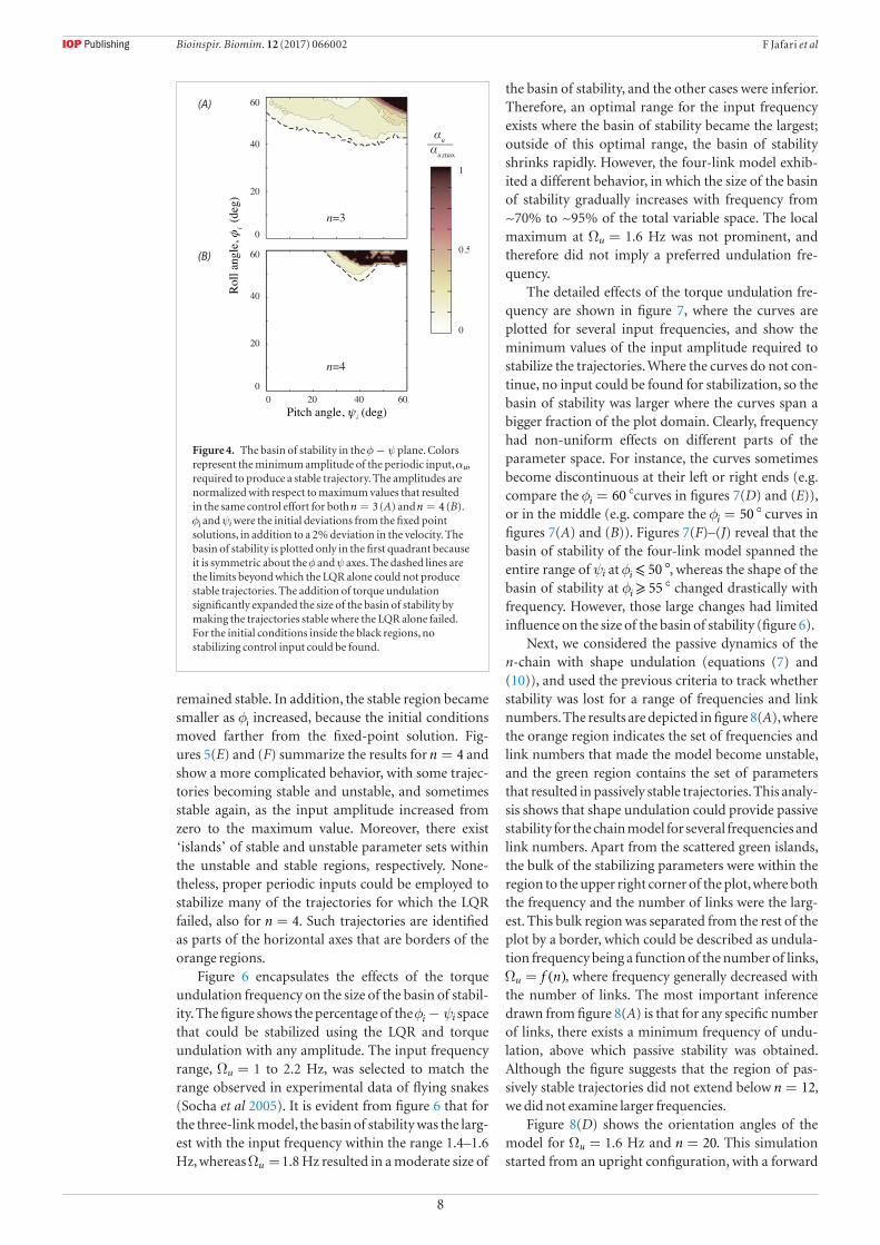
Figure 4 depicts the basin of stability in the φ ψ− plane with colors representing the minimum ampl-itude of the periodic input, αu (see equation (6)), required to have a stable trajectory. The amplitudes are normalized with respect to the maximum value used for the simulations. It is important to mention here that the plots show only a subset of the basin of stabil-ity, which has the same dimensions as the state space. Because we are concerned with the orientation stabil-ity, only the φ ψ− section is considered. Although the maximum amplitude for =n 3 and =n 4 were differ-ent, they were selected such that they resulted in the same control effort, defined as the average torque at the joints (see appendix). The initial deviations from the fixed point solutions were φi

and ψi, in addition to a 2% deviation in the velocity. We defined a trajectory to have not diverged, if neither φ nor ψ reached 80° dur-ing a 15 s simulation, which was long enough for any instabilities to manifest. It should be noted that the basin of stability is plotted only in the first quadrant because it is symmetric about the φ and ψ axes. Inspec-tion shows that the curves would produce cusps at the axes when symmetrically reflected in them.

It is evident from figure 4 that the LQR could pro-vide stability only for a finite portion of the shown space. When the initial angles went far away from the fixed-point solution, the stabilization by the LQR

alone failed, but many of the trajectories could be sta-bilized with the addition of torque undulation. In the three-link model, φi mainly determined whether the LQR alone was sufficient for stability, and φ = °40i was the approximate border for the periodic inputs being required for stability. The four-link model had a more complex behavior, with both φi and ψi playing roles to determine where the LQR alone stabilized the trajecto-ries. Also, stabilization of the trajectories with farther initial conditions generally required larger amplitudes of torque undulation. However, this method could not be used without limits either, as the dark regions in fig-ure 4 show there exist initial conditions for which no stable trajectories could be found. Nevertheless, using torque undulation, we could significantly expand the basin of stability, particularly for =n 3.

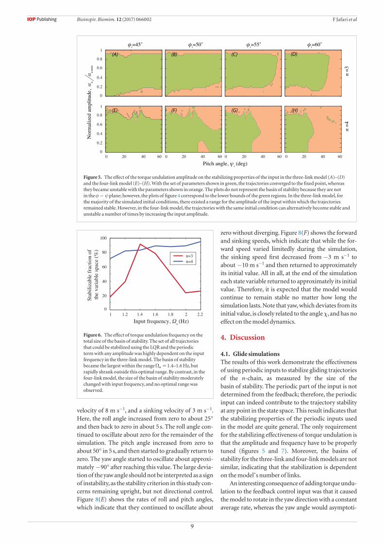
Next, we explored how the amplitude and fre-quency of torque undulation influenced its stabilizing properties. Figure 5 shows how different torque undu-lation amplitudes caused the trajectories starting from various φi and ψi to converge to the fixed point (green regions) or to become unstable (orange regions). As before, a trajectory was considered unstable if either φ or ψ reached 80° during a 15 s simulation. Note that the regions shown in figure 5 are not plotted in the φ ψ− plane and should not be confused with the basin of stability. Figures 5(A)–(D) summarize the results for =n 3 and indicate that for the majority of the simu-

lated initial conditions, there exists a range for the amplitude of the input within which the trajectories

Figure 3. The fixed-point solutions of the n-chain model with three and four links. (A) and (B) The model shape and the in-plane component of the fixed-point velocities. The axis of gravity is perpendicular to the figure plane. Simulations for the model orientation (C) and (D), and CoM velocities (E) and (F). Using the LQR to stabilize the fixed point, the trajectories with the initial conditions of φ = °30i , ψ = °40i , and a 2% deviation in the initial velocity converged to the fixed point (solid lines). The state variables starting from the same initial condition, but with torque undulation, converged to oscillating about the fixed-point solution without becoming unstable (dashed lines). The yaw angle, which was not a state variable, and therefore was not controllable, started to decrease or increase with time when the periodic term was added to the input. Supplementary movie 1 (available at stacks.iop.org/BB/12/066002/mmedia) shows the animation of the simulation in figures (C) and (E) with torque undulation.

Bioinspir. Biomim. 12 (2017) 066002

8

F Jafari et al

remained stable. In addition, the stable region became smaller as φi increased, because the initial conditions moved farther from the fixed-point solution. Fig-ures 5(E) and (F) summarize the results for =n 4 and show a more complicated behavior, with some trajec-tories becoming stable and unstable, and sometimes stable again, as the input amplitude increased from zero to the maximum value. Moreover, there exist ‘islands’ of stable and unstable parameter sets within the unstable and stable regions, respectively. None-theless, proper periodic inputs could be employed to stabilize many of the trajectories for which the LQR failed, also for =n 4. Such trajectories are identified as parts of the horizontal axes that are borders of the orange regions.

Figure 6 encapsulates the effects of the torque undulation frequency on the size of the basin of stabil-ity. The figure shows the percentage of the φ ψ−i i space that could be stabilized using the LQR and torque undulation with any amplitude. The input frequency range, Ω =u 1 to 2.2 Hz, was selected to match the range observed in experimental data of flying snakes (Socha et al 2005). It is evident from figure 6 that for the three-link model, the basin of stability was the larg-est with the input frequency within the range 1.4–1.6 Hz, whereas Ω =u 1.8 Hz resulted in a moderate size of

the basin of stability, and the other cases were inferior. Therefore, an optimal range for the input frequency exists where the basin of stability became the largest; outside of this optimal range, the basin of stability shrinks rapidly. However, the four-link model exhib-ited a different behavior, in which the size of the basin of stability gradually increases with frequency from ~70% to ~95% of the total variable space. The local maximum at Ω =u 1.6 Hz was not prominent, and therefore did not imply a preferred undulation fre-quency.

The detailed effects of the torque undulation fre-quency are shown in figure 7, where the curves are plotted for several input frequencies, and show the minimum values of the input amplitude required to stabilize the trajectories. Where the curves do not con-tinue, no input could be found for stabilization, so the basin of stability was larger where the curves span a bigger fraction of the plot domain. Clearly, frequency had non-uniform effects on different parts of the parameter space. For instance, the curves sometimes become discontinuous at their left or right ends (e.g. compare the φ = °60i curves in figures 7(D) and (E)), or in the middle (e.g. compare the φ = °50i curves in figures 7(A) and (B)). Figures 7(F)–(J) reveal that the basin of stability of the four-link model spanned the entire range of ψi at ⩽φ °50i , whereas the shape of the basin of stability at ⩾φ °55i changed drastically with frequency. However, those large changes had limited influence on the size of the basin of stability (figure 6).

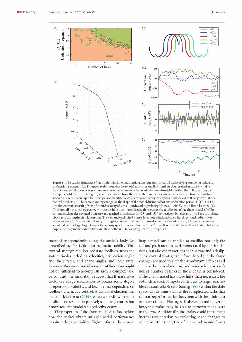
Next, we considered the passive dynamics of the n-chain with shape undulation (equations (7) and (10)), and used the previous criteria to track whether stability was lost for a range of frequencies and link numbers. The results are depicted in figure 8(A), where the orange region indicates the set of frequencies and link numbers that made the model become unstable, and the green region contains the set of parameters that resulted in passively stable trajectories. This analy-sis shows that shape undulation could provide passive stability for the chain model for several frequencies and link numbers. Apart from the scattered green islands, the bulk of the stabilizing parameters were within the region to the upper right corner of the plot, where both the frequency and the number of links were the larg-est. This bulk region was separated from the rest of the plot by a border, which could be described as undula-tion frequency being a function of the number of links,

( )Ω = f nu , where frequency generally decreased with the number of links. The most important inference drawn from figure 8(A) is that for any specific number of links, there exists a minimum frequency of undu-lation, above which passive stability was obtained. Although the figure suggests that the region of pas-sively stable trajectories did not extend below =n 12, we did not examine larger frequencies.

Figure 8(D) shows the orientation angles of the model for Ω =u 1.6 Hz and =n 20. This simulation started from an upright configuration, with a forward

Figure 4. The basin of stability in the φ ψ− plane. Colors represent the minimum amplitude of the periodic input, αu, required to produce a stable trajectory. The amplitudes are normalized with respect to maximum values that resulted in the same control effort for both =n 3 (A) and =n 4 (B). φi and ψi were the initial deviations from the fixed point solutions, in addition to a 2% deviation in the velocity. The basin of stability is plotted only in the first quadrant because it is symmetric about the φ and ψ axes. The dashed lines are the limits beyond which the LQR alone could not produce stable trajectories. The addition of torque undulation significantly expanded the size of the basin of stability by making the trajectories stable where the LQR alone failed. For the initial conditions inside the black regions, no stabilizing control input could be found.

Bioinspir. Biomim. 12 (2017) 066002

9

F Jafari et al

velocity of 8 m s−1, and a sinking velocity of 3 m s−1. Here, the roll angle increased from zero to about 25° and then back to zero in about 5 s. The roll angle con-tinued to oscillate about zero for the remainder of the simulation. The pitch angle increased from zero to about 50° in 5 s, and then started to gradually return to zero. The yaw angle started to oscillate about approxi-mately −90° after reaching this value. The large devia-tion of the yaw angle should not be interpreted as a sign of instability, as the stability criterion in this study con-cerns remaining upright, but not directional control. Figure 8(E) shows the rates of roll and pitch angles, which indicate that they continued to oscillate about

zero without diverging. Figure 8(F) shows the forward and sinking speeds, which indicate that while the for-ward speed varied limitedly during the simulation, the sinking speed first decreased from −3 m s−1 to about −10 m s−1 and then returned to approximately its initial value. All in all, at the end of the simulation each state variable returned to approximately its initial value. Therefore, it is expected that the model would continue to remain stable no matter how long the simulation lasts. Note that yaw, which deviates from its initial value, is closely related to the angle χ, and has no effect on the model dynamics.

4. Discussion

4.1. Glide simulationsThe results of this work demonstrate the effectiveness of using periodic inputs to stabilize gliding trajectories of the n-chain, as measured by the size of the basin of stability. The periodic part of the input is not determined from the feedback; therefore, the periodic input can indeed contribute to the trajectory stability at any point in the state space. This result indicates that the stabilizing properties of the periodic inputs used in the model are quite general. The only requirement for the stabilizing effectiveness of torque undulation is that the amplitude and frequency have to be properly tuned (figures 5 and 7). Moreover, the basins of stability for the three-link and four-link models are not similar, indicating that the stabilization is dependent on the model’s number of links.

An interesting consequence of adding torque undu-lation to the feedback control input was that it caused the model to rotate in the yaw direction with a constant average rate, whereas the yaw angle would asymptoti-

Figure 5. The effect of the torque undulation amplitude on the stabilizing properties of the input in the three-link model (A)–(D) and the four-link model (E)–(H). With the set of parameters shown in green, the trajectories converged to the fixed point, whereas they became unstable with the parameters shown in orange. The plots do not represent the basin of stability because they are not in the φ ψ− plane; however, the plots of figure 4 correspond to the lower bounds of the green regions. In the three-link model, for the majority of the simulated initial conditions, there existed a range for the amplitude of the input within which the trajectories remained stable. However, in the four-link model, the trajectories with the same initial condition can alternatively become stable and unstable a number of times by increasing the input amplitude.

Figure 6. The effect of torque undulation frequency on the total size of the basin of stability. The set of all trajectories that could be stabilized using the LQR and the periodic term with any amplitude was highly dependent on the input frequency in the three-link model. The basin of stability became the largest within the range Ω =u 1.4–1.6 Hz, but rapidly shrank outside this optimal range. By contrast, in the four-link model, the size of the basin of stability moderately changed with input frequency, and no optimal range was observed.

Bioinspir. Biomim. 12 (2017) 066002

10

F Jafari et al

cally converge to some constant value in the absence of the periodic input. As explained earlier, the reason for this behavior is that angle χ, which becomes the same as the yaw angle at the fixed point, is cyclic and unactu-ated; therefore, it is not controlled and is expected to be influenced by any perturbation including the periodic inputs. As a result, the model lacks directional control, and disturbances change its direction of motion. On the other hand, the effect of the periodic input on the yaw angle is predictable and constant in average, making it possible for torque undulation to be used as a simple means to ‘drive’ the model in the yaw direction. Upon reaching the desired direction, the periodic inputs are ‘turned off’, after which all variables including the yaw rate will dissipate and go to zero, and the system pro-ceeds with the new direction.

The periodic motions in the controlled glide simulations are small-amplitude compared to real undulation in flying snakes. These small-amplitude motions cause the model to wobble about the fixed-point shape, which is asymmetric about any axis (fig-ure 3 and supplementary video 1). By contrast, high- ampl itude waves of shape undulation provide average symmetry about the fore-aft axis, which should mini-mize the control requirements. In addition, accord-ing to the theory of vibrational control, undulation is a zero-mean periodic input to the system and may be able to provide open-loop stability. The simulations of the passive dynamics of the model with shape undula-tion suggest that it could indeed provide stability with-out any feedback. Our results are also in accordance with the averaging theorem, as they indicate that sta-bility is obtained for any undulation frequency above a certain value. The minimum required frequency is a generally decreasing function of the number of links, which suggests that a lager number of links, or equiva-

lently smoother shape changes, helps to produce stabil-ity. Moreover, because power consumption is propor-tional to the square of frequency, with a larger number of links, stability is obtained at a lower energy cost.

Figure 8(A) shows that some low-frequency undu-latory motions can also lead to passive stability, even at zero frequency ( =n 6). However, these low-frequency motions are scattered and separate from the compact set of high-frequency parameters. Such scattered param-eters could not be predicted by the averaging theorem, but they have been studied in some simple mechanical systems (Berg and Wickramasinghe 2015). Figure 8(A) also suggests that a minimum number of links is needed to obtain passive stability with shape undulation. Testing this hypothesis requires analyzing the model at higher frequencies, which was not done in this work. However, it is noteworthy that some other mechanical systems, namely boomerangs, are made of as few as two rigidly connected airfoils and fly through the air with near zero rates of roll and pitch, but they use high spin rates instead of shape reconfigurations (Azuma et al 2004).

4.2. Implications about gliding snakesOur first hypothesis about why flying snakes undulate when airborne was that undulation is a necessary condition for stable gliding. The results obtained from the controlled glide simulations do not support the hypothesis, as stabilizable fixed points in the state space do exist, to which the trajectories converged asymptotically. This analysis shows that stable trajectories could be obtained with a minimum number of three airfoils in the model. Therefore, it is theoretically possible for the airborne snakes to hold a static posture and still glide, provided that the snakes have sufficient postural control to dissipate disturbances. For instance, fine locomotor control

Figure 7. The effects of torque undulation frequency on the shape of the basin of stability. The curves show the minimum values of the input amplitude required to stabilize the trajectories, so the curves at Ωu = 1.4 Hz correspond to the lower bounds of the green regions in figure 5. Where the curves are discontinuous, no stabilizing input could be found. The shape of the basin of stability changed nonuniformly with the input frequency for both =n 3 and =n 4. The curves became discontinuous at their left or right ends (e.g. φ = °60i curves in (D) and (E)), or in the middle (e.g. φ = °50i curves in (A) and (F)). For =n 4, the basin of stability spanned the entire range of ψi at ⩽φ °50i , but became dependent on the frequency at ⩾φ °55i (F)–(J).

Bioinspir. Biomim. 12 (2017) 066002

11

F Jafari et al

executed independently along the snake’s body (as prescribed by the LQR) can maintain stability. This control strategy requires accurate feedback from the state variables including velocities, orientation angles and their rates, and shape angles and their rates. However, the neuromuscular system of the snakes might not be sufficient to accomplish such a complex task. By contrast, the simulations suggest that flying snakes could use shape undulation to obtain some degree of open-loop stability, and become less dependent on feedback and active control. A similar deduction was made in Jafari et al (2014), where a model with some idealizations resulted in passively stable trajectories, but a more realistic model required active control.

The properties of the chain model can also explain how the snakes obtain an agile aerial performance despite lacking specialized flight surfaces. The closed-

loop control can be applied to stabilize not only the roll and pitch motions as demonstrated by our simula-tions, but also other motions such as yaw and sideslip. These control strategies are force-based (i.e. the shape changes are used to alter the aerodynamic forces and achieve the desired motion) and work as long as a suf-ficient number of links in the n-chain is considered. If the chain model has more links than necessary, the redundant control inputs contribute to larger reacha-ble and controllable sets (Sontag 1998) within the state space, which translate into the complicated tasks that cannot be performed by the system with the minimum number of links. Having well above a hundred verte-brae, the snakes may be able to perform maneuvers in this way. Additionally, the snakes could implement inertial reorientation by exploiting shape changes to rotate in 3D irrespective of the aerodynamic forces

Figure 8. The passive dynamics of the model with kinematic undulation (equation (7)), and with varying number of links and undulation frequency. (A) The green region contains the set of frequencies and link numbers that resulted in passively stable trajectories, and the orange region contains the set of parameters that made the model unstable. Within the bulk green region to the upper right corner of the figure, which is separated from the rest of the parameter space with the hatched band, undulation worked as a zero-mean input to render passive stability above a certain frequency for any link number, as the theory of vibrational control predicts. (B) The corresponding changes in the shape of the model during half of one undulation period, T. (C)–(F) The simulation results starting from a forward velocity of 8 m s−1, and a sinking velocity of 3 m s−1, with Ω =u 1.6 Hz and =n 20. (C) The three-dimensional trajectory, with the position axes normalized with respect to the total length of the chain model. (D) The roll and pitch angles deviated from zero and reached a maximum of ~25° and ~50°, respectively, but they returned back to oscillate about zero during the simulation time. The yaw angle exhibited a large deviation, which indicates that directional stability was not achieved. (E) The rates of roll and pitch angles, showing that they continued to oscillate about zero. (F) Although the forward speed did not undergo large changes, the sinking speed decreased from −3 m s−1 to −10 m s−1 and returned back to its initial value. Supplementary movie 2 shows the animation of the simulation in figures (C) through (F).

Bioinspir. Biomim. 12 (2017) 066002

12

F Jafari et al

(e.g. Walsh and Sastry (1995) and Kolmanovsky et al (1995)). In this regard, the induced rotation is similar to the righting of lizards using tail inertia (Jusufi et al 2010) and certain bat maneuvers using wing inertia (Bergou et al 2015). With inertial reorientation, the snakes can perform maneuvers that are not observed in other gliders, such as sharp turning at low speeds and turning without banking (Socha 2002). Therefore, this study suggests that the snakes can accomplish multi-ple maneuvers because of their relatively unrestrained ability for postural changing, which is enabled by their musculoskeletal design. In other words, a seemingly poor body design—cylindrical with no appendages—turns out to be a versatile asset.

4.3. Modeling limitationsThe theoretical analysis in this work entails the assumptions of the model, suggesting multiple limitations of this study.

1. Despite limited data about the aerodynamic interaction between the fore and the aft body of the snake (Miklasz et al 2010), it is likely that the flow structures created upstream are intercepted by the downstream body, producing some aerodynamic coupling, at least at some points in the glide trajectory. Because limited data are available, as a first-order approximation, each model link was assumed to be aerodynamically uncoupled from the links before and after. Moreover, we neglected aerodynamic end effects, such as tip vortices or effects due to the low aspect ratio of the airfoils. However, the robustness of the model stabilizations suggests that such aerodynamic effects may have only a minor influence on the basin of stability.

2. The model assumes that the links are uniform, whereas the real snake displays varying morphology along the body length. In particular, the width of the body is non-uniform, being maximal at mid-body and tapering toward the tail, and the cross-sectional shape may not be constant. Such differences will alter slightly the lift and drag experienced by each link.

3. The model did not simulate the beginning part of the glide trajectory, when the speeds are small and the snake’s undulating configuration is not yet formed. In practice, any simulation starting from small initial velocities would result in instability, and the stable trajectories could be obtained only with sufficiently large initial velocities. As discussed in Jafari et al (2014), this part of the glide involves kinematics that are likely to produce different aerodynamic forces than those in the developed phase of the glide.

4.4. ConclusionsIn this study, we used theoretical modeling to understand the role of undulation in the dynamics of

snake gliding flight. We simulated trajectories of the n-chain model about its biomechanically relevant fixed-point solutions for =n 3 and =n 4. A linearization-based stability analysis showed that the fixed-point solutions were unstable, but could be stabilized using joint torques as inputs. Although the stabilization was not accomplished globally, it was effective for a considerable portion of the state space that was pertinent to the biologically relevant kinematics of flying snakes. Further exploration revealed that by adding torque undulation about the fixed-point shape, the size of the basin of stability significantly expanded. Moreover, simulations with shape undulation demonstrated that open-loop stability could be obtained with a sufficiently large frequency of undulation. Overall, this study demonstrates the possibility of maintaining stability during gliding using a morphing body instead of symmetrically paired wings. Furthermore, undulation lowers the demand for a complex closed-loop control system by allowing it to be formed about a passively stable trajectory.

The results of this study help to understand the fundamental control mechanisms that snakes employ during a glide. We determined the minimum func-tional requirements for the stability of snake gliding; therefore, our findings could provide insight into the evolutionary transitions that have led to such a unique behavior. Furthermore, by studying the gliding behav-ior of snakes, it may be possible to learn a novel method of implementing vibrational control in a flying air or water vehicle. Finally, the dynamical framework we have developed allows us to explore theoretically possible but biologically unrealized motions, and to exploit the underlying principles to engineer biologi-cally inspired robotic analogues to snakes. However, for robotic applications, weight and power limitations have to be carefully considered, as the required power substantially increases with weight. In particular, the open-loop kinematic undulations were simulated based on the assumption that any required joint tor-ques could be supplied. So, it is possible that the stabi-lizing properties of undulation could be used to design a snake-like flyer if actuators with sufficiently small weight-to-power ratios are available.

Refinements of this model would be served by incorporating more accurate representation of the snake’s 3D kinematics, as well as understanding the full aerodynamics of the snake’s cross-sectional shape throughout the body. A study is currently underway to determine the behavior of two snake-like 2D air-foils placed in tandem (Jafari et al in preparation), but the effects of low aspect ratio, unsteady motions, and sweep angle remain unexplored. Experiments in which the snakes are perturbed in their glide, or with robotic models, are needed to verify these theor etical results. The methods of this work may be useful to study other aspects of snake flight including the dynamics of turn-ing or the effects of shape kinematics on the trajectory. Moreover, a similar approach can be applied to limb-

Bioinspir. Biomim. 12 (2017) 066002

13

F Jafari et al

less motion through any fluid, for example with the swimming of eels (Tytell et al 2010).

Acknowledgments

This work was supported in part by the National Science Foundation under awards 1150456 and 1537349 to SDR and 1351322 to JJS. The authors would like to thank two anonymous reviewers for their constructive and fruitful suggestions.

Appendix. Normalizing the periodic input amplitude based on the control effort

To be able to properly compare the simulation results for models with different numbers of links, we need to obtain a measure of the control effort independent of n. Because the n-chain model is an attempt to approximate the waveform of the real snake, we assume a sinusoidal variation of torque along the body. Such an approximation satisfies the boundary conditions at the head and tail points of the model, which are free, indicating zero torque at those points. Based on this estimation, the appropriate form of the joint torques is expressed as

τ τ π ν π ω= −t j n j n tsinj 0 ( ) ( )( ) (A.1)

where ( )ν ⋅ is some bounded periodic function, and

( )τ τ π= j nsinj 0 (A.2)

is the jth joint torque amplitude, with τ0 being some reference value. Therefore, the joint torques can vary as periodic functions of time representing a traveling wave. A similar approximation was used in Hirose and Yamada (2009) for the terrestrial locomotion of a snake-like robot.

If we define the control effort as the RMS value of the joint torque amplitudes using equation (A.2), it can be shown that

∑τ τ τ= =n

1 2

2jjrms2

0 (A.3)

which is independent of the number of links.Therefore, we normalized the amplitude of torque

undulation for the models with different numbers of links, with respect to the reference amplitude for each n that resulted in the same control effort.

ORCID iDs

Farid Jafari https://orcid.org/0000-0003-3252-5111

References

Alexander R M 2003 Principles of Animal Locomotion (Princeton, NJ: Princeton University Press)

Azuma A, Beppu G, Ishikawa H and Yasuda K 2004 Flight dynamics of the boomerang, part 1: fundamental analysis J. Guid. Control Dynam. 27 545–54

Baruh H 1999 Analytical Dynamics (New York: McGraw-Hill)Berg J M and Wickramasinghe I M 2015 Vibrational control

without averaging Automatica 58 72–81Bergou A J, Swartz S M, Vejdani H, Riskin D K, Reimnitz L,

Taubin G and Breuer K S 2015 Falling with style: bats perform complex aerial rotations by adjusting wing inertia PLoS Biol. 13 e1002297

Biewener A A 2003 Animal Locomotion (Oxford: Oxford University Press)

Boltz F W, Kenyon G C and Allen C Q 1960 Effects of sweep angle on the boundary-layer stability characteristics of an untapered wing at low speeds Technical Report NASA-TN-D-338

Bullo F 2002 Averaging and vibrational control of mechanical systems SIAM J. Control Optim. 41 542–62

Chernousko F L 2005 Modelling of snake-like locomotion Appl. Math. Comput. 164 415–34

Dormand J R and Prince P J 1980 A family of embedded Runge–Kutta formulae J. Comput. Appl. Math. 6 19–26

Dowling K 1999 Limbless locomotion: learning to crawl Proc. 1999 IEEE Int. Conf. on Robotics and Automation vol 4 (IEEE) pp 3001–6

Ellington C 1984 The aerodynamics of hovering insect flight. I. The quasi-steady analysis Phil. Trans. R. Soc. London. B 305 1–15

Enner F, Rollinson D and Choset H 2012 Simplified motion modeling for snake robots 2012 IEEE Int. Conf. on Robotics and Automation (ICRA) (IEEE) pp 4216–21

Grizzle J, Moog C H and Chevallereau C 2005 Nonlinear control of mechanical systems with an unactuated cyclic variable IEEE Trans. Autom. Control 50 559–76

Guckenheimer J and Holmes P 2013 Nonlinear Oscillations, Dynamical Systems, and Bifurcations of Vector Fields (Berlin: Springer)

Hirose S and Morishima A 1990 Design and control of a mobile robot with an articulated body Int. J. Robot. Res. 9 99–114

Hirose S and Yamada H 2009 Snake-like robots IEEE Robot. Autom. Mag. 16 88–98

Holden D, Socha J J, Cardwell N D and Vlachos P P 2014 Aerodynamics of the flying snake Chrysopelea paradisi: how a bluff body cross-sectional shape contributes to gliding performance J. Exp. Biol. 217 382–94

Jafari F, Ross S D, Vlachos P P and Socha J J 2014 A theoretical analysis of pitch stability during gliding in flying snakes Bioinspir. Biomim. 9 025014

Jones R T 1947 Effects of sweepback on boundary layer and separation Technical Report NACA-TR-884

Jusufi A, Kawano D, Libby T and Full R 2010 Righting and turning in mid-air using appendage inertia: reptile tails, analytical models and bio-inspired robots Bioinspir. Biomim. 5 045001

Kane T R and Levinson D A 1985 Dynamics, Theory and Applications (New York: McGraw-Hill)

Kapitza P 1951 Dynamic stability of a pendulum with an oscillating point of suspension J. Exp. Theor. Phys. 21 588–97

Kolmanovsky I, McClamroch N and Coppola V 1995 New results on control of multibody systems which conserve angular momentum J. Dyn. Control Syst. 1 447–62

Liljebäck P, Pettersen K Y, Stavdahl Ø and Gravdahl J T 2010 Stability analysis of snake robot locomotion based on averaging theory 2010 49th IEEE Conf. on Decision and Control (CDC) (IEEE) pp 1977–84

Maladen R D, Ding Y, Umbanhowar P B and Goldman D I 2011 Undulatory swimming in sand: experimental and simulation studies of a robotic sandfish Int. J. Robot. Res. 30 793–805

Meerkov S M 1980 Principle of vibrational control: theory and applications IEEE Trans. Autom. Control 25 755–62

Miklasz K, Labarbera M, Chen X and Socha J 2010 Effects of body cross-sectional shape on flying snake aerodynamics Exp. Mech. 50 1335–48

Morgansen K A, Vela P A and Burdick J W 2002 Trajectory stabilization for a planar carangiform robot fish Proc. IEEE Int. Conf. on Robotics and Automation, 2002 (ICRA’02) (IEEE) pp 756–62

Bioinspir. Biomim. 12 (2017) 066002

14

F Jafari et al

Mori M and Hirose S 2002 Three-dimensional serpentine motion and lateral rolling by active cord mechanism ACM-R3 IEEE/RSJ Int. Conf. on Intelligent Robots and Systems (IEEE) pp 829–34

Prautsch P and Mita T 1999 Control and analysis of the gait of snake robots Proc. of the 1999 IEEE Int. Conf. on Control Applications (IEEE) pp 502–7

Saito M, Fukaya M and Iwasaki T 2002 Modeling, analysis, and synthesis of serpentine locomotion with a multilink robotic snake IEEE Control Syst. Mag. 22 64–81

Schlichting H and Truckenbrodt E 1979 Aerodynamics of the Aeroplane (New York: McGraw Hill)

Socha J J 2002 Kinematics: gliding flight in the paradise tree snake Nature 418 603–4

Socha J J 2006 Becoming airborne without legs: the kinematics of take-off in a flying snake, Chrysopelea paradisi J. Exp. Biol. 209 3358–69

Socha J J 2011 Gliding flight in Chrysopelea: turning a snake into a wing Integr. Comput. Biol. 51 969–82

Socha J J, Jafari F, Munk Y and Byrnes G 2015 How animals glide: from trajectory to morphology Can. J. Zool. 93 901–24

Socha J J and Labarbera M 2005 Effects of size and behavior on aerial performance of two species of flying snakes (Chrysopelea) J. Exp. Biol. 208 1835–47

Socha J J, Miklasz K, Jafari F and Vlachos P P 2010 Non-equilibrium trajectory dynamics and the kinematics of gliding in a flying snake Bioinspir. Biomim. 5 045002

Socha J J, O’Dempsey T and Labarbera M 2005 A 3D kinematic analysis of gliding in a flying snake, Chrysopelea paradisi J. Exp. Biol. 208 1817–33

Sontag E D 1998 Mathematical Control Theory: Deterministic Finite Dimensional Systems (Berlin: Springer)

Taha H E, Tahmasian S, Woolsey C A, Nayfeh A H and Hajj M R 2015 The need for higher-order averaging in the stability analysis of hovering, flapping-wing flight Bioinspir. Biomim. 10 016002

Tahmasian S and Woolsey C A 2015 A control design method for underactuated mechanical systems using high-frequency inputs J. Dynam. Syst. Meas. Control 137 071004

Tahmasian S, Woolsey C A and Taha H E 2014 Longitudinal flight control of flapping wing micro air vehicles AIAA Guidance, Navigation, and Control Conf., AIAA SciTech Forum AIAA 2014-1470 (https://doi.org/10.2514/6.2014-1470)

Thomsen J J 2005 Slow high-frequency effects in mechanics: problems, solutions, potentials Int. J. Bifurcation Chaos 15 2799–818

Tytell E D, Hsu C-Y, Williams T L, Cohen A H and Fauci L J 2010 Interactions between internal forces, body stiffness, and fluid environment in a neuromechanical model of lamprey swimming Proc. Natl Acad. Sci. USA 107 19832–7

Walsh G C and Sastry S S 1995 On reorienting linked rigid bodies using internal motions IEEE Trans. Robot. Autom. 11 139–46

Bioinspir. Biomim. 12 (2017) 066002