control factors and scale analysis of annual river water ... factors and scale analysis of annual...

1

Supplementary Information

Control factors and scale analysis of annual river water, sediments and carbon

transport in China

Chunlin Song1, 2, Genxu Wang*1, Xiangyang Sun1, Ruiying Chang1, Tianxu Mao1, 2

1Institute of Mountain Hazards and Environment, Chinese Academy of Sciences, Chengdu, 610041, China

2University of Chinese Academy of Sciences, Beijing, 100049, China

*Correspondence to: [email protected](Genxu Wang).

Mean(Sample Size)

Small Medium Sizeable Large Great

TSSC(mg/L) 3239(33) 3187(59) 843(53) 1523(59) 3430(55)

TSSL(g·m-2·a-1) 768(58) 254(64) 271(54) 237(55) 254(62)

POCC(mg/L) 76.73(12) 15.55(19) 25.59(7) 7.94(18) 25.56(10)

POCL(g·m-2·a-1) 0.88(26) 4.27(20) 1.49(7) 2.87(19) 1.07(16)

DOCC(mg/L) 4.49(11) 2.73(17) 3.95(5) 3.22(18) 3.01(9)

DOCL(g·m-2·a-1) 1.20(25) 2.99(19) 1.01(5) 1.56(19) 0.34(14)

Rc 0.36(63) 0.46(72) 0.33(55) 0.39(65) 0.32(62)

Size (km2) 5522(63) 47179(72) 172035(55) 466285(65) 1192080(62)

L (km) 181(63) 634(72) 1275(55) 2400(65) 5227(62)

RD (mm) 463(63) 670(72) 312(55) 461(65) 313(62)

QA (m3/s) 62(63) 925(72) 1676(55) 6313(65) 14301(62)

MAP (mm) 1060.6(63) 1212.4(72) 846.4(55) 1047.1(65) 802.9(62)

MAT (°C) 15.8(63) 15.1(72) 10.8(55) 12.3(65) 11.9(62)

S (%) 9.34(50) 1.79(72) 1.26(55) 0.90(65) 1.01(62)

Vc (%) 33.20(11) 45.04(26) 23.30(20) 29.19(23) 27.45(24)

RSCI (%) 20.72(3) 46.74(19) 42.75(29) 27.38(35) 73.45(48)

SOC (%) 1.37(58) 1.06(11) 1.25(3) 0.97(3) \

BD (g/cm3) 1.27(58) 1.29(11) 1.27(3) 1.29(3) \

Table S1. General statistics for the variables in different scales (Small, Medium, Sizeable, Large, Great). Sample size

is given is brackets. Abbreviations of the variables as shows in Table 1.

2

Figure S1. The age distribution of trials of our database.

3

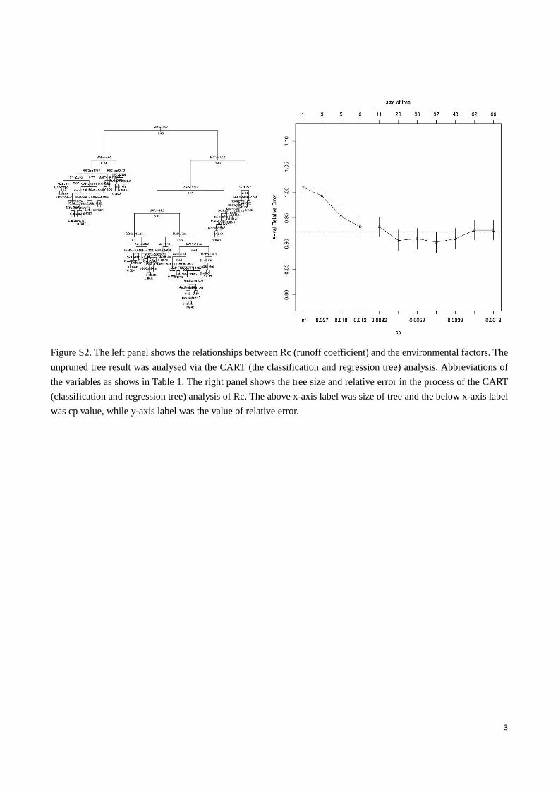
Figure S2. The left panel shows the relationships between Rc (runoff coefficient) and the environmental factors. The

unpruned tree result was analysed via the CART (the classification and regression tree) analysis. Abbreviations of

the variables as shows in Table 1. The right panel shows the tree size and relative error in the process of the CART

(classification and regression tree) analysis of Rc. The above x-axis label was size of tree and the below x-axis label

was cp value, while y-axis label was the value of relative error.

4

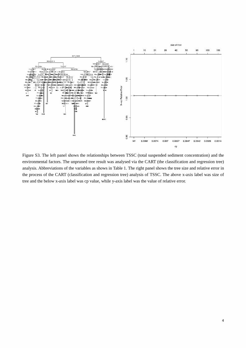
Figure S3. The left panel shows the relationships between TSSC (total suspended sediment concentration) and the

environmental factors. The unpruned tree result was analysed via the CART (the classification and regression tree)

analysis. Abbreviations of the variables as shows in Table 1. The right panel shows the tree size and relative error in

the process of the CART (classification and regression tree) analysis of TSSC. The above x-axis label was size of

tree and the below x-axis label was cp value, while y-axis label was the value of relative error.

5

Figure S4. The left panel shows the relationships between TSSL (total suspended sediment load) and the

environmental factors. The unpruned tree result was analysed via the CART (the classification and regression tree)

analysis. Abbreviations of the variables as shows in Table 1. The right panel shows the tree size and relative error in

the process of the CART (classification and regression tree) analysis of TSSL. The above x-axis label was size of tree

and the below x-axis label was cp value, while y-axis label was the value of relative error.

6

Figure S5. The left panel shows the relationships between TOCL (total organic carbon load) and the environmental

factors. The unpruned tree result analysed via the CART (the classification and regression tree) analysis.

Abbreviations of the variables as shows in Table 1. The right panel shows the tree size and relative error in the process

of the CART (classification and regression tree) analysis of TOCL. The above x-axis label was size of tree and the

below x-axis label was cp value, while y-axis label was the value of relative error.

7

Figure S6. Diagnostic plots for the regression model of Rc on MAP and MAT.

8

Figure S7. Diagnostic plots for the regression model of TSSC on MAP, RSCI, RD, S, and Vc.

9

Figure S8. Diagnostic plots for the regression model of TSSL on RSCI, RD, MAP, MAT, and Vc.

10

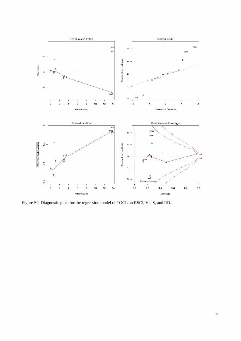
Figure S9. Diagnostic plots for the regression model of TOCL on RSCI, Vc, S, and RD.

11

Figure S10. Boxplot of TSSL and TOCL in different classes of Vc.

12

Figure S11. Boxplot of TSSL and TOCL in different classes of RSCI.

13

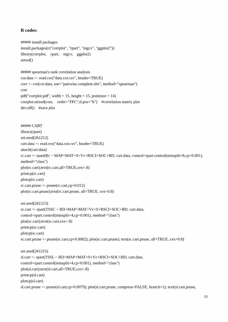
R codes:

##### install packages

install.packages(c("corrplot", "rpart", "mgcv", "ggplot2"))

library(corrplot, rpart, mgcv, ggplot2)

setwd()

##### spearman's rank correlation analysis

cor.data <- read.csv("data.cor.csv", header=TRUE)

corr <- cor(cor.data, use="pairwise.complete.obs", method="spearman")

corr

pdf("corrplot.pdf", width = 15, height = 15, pointsize = 14)

corrplot.mixed(corr, order="FPC",tl.pos="lt") #correlation matrix plot

dev.off() #save plot

##### CART

library(rpart)

set.seed(261212)

cart.data <- read.csv("data.cor.csv", header=TRUE)

attach(cart.data)

rc.cart <- rpart(Rc ~ MAP+MAT+S+Vc+RSCI+SOC+BD, cart.data, control=rpart.control(minsplit=8,cp=0.001),

method="class")

plot(rc.cart);text(rc.cart,all=TRUE,cex=.8)

printcp(rc.cart)

plotcp(rc.cart)

rc.cart.prune <- prune(rc.cart,cp=0.012)

plot(rc.cart.prune);text(rc.cart.prune, all=TRUE, cex=0.8)

set.seed(261213)

sc.cart <- rpart(TSSC ~ RD+MAP+MAT+Vc+S+RSCI+SOC+BD, cart.data,

control=rpart.control(minsplit=4,cp=0.001), method="class")

plot(sc.cart);text(sc.cart,cex=.8)

printcp(sc.cart)

plotcp(sc.cart)

sc.cart.prune <- prune(sc.cart,cp=0.0082); plot(sc.cart.prune); text(sc.cart.prune, all=TRUE, cex=0.8)

set.seed(261215)

sl.cart <- rpart(TSSL ~ RD+MAP+MAT+S+Vc+RSCI+SOC+BD, cart.data,


plot(sl.cart);text(sl.cart,all=TRUE,cex=.8)

printcp(sl.cart)

plotcp(sl.cart)

sl.cart.prune <- prune(sl.cart,cp=0.0079); plot(sl.cart.prune, compress=FALSE, branch=1); text(sl.cart.prune,

14

all=TRUE, cex=0.8)

set.seed(261216)

set.seed(271702)

oc.cart <- rpart(TOCL ~ RD+MAP+MAT+S+Vc+RSCI+SOC+BD, cart.data,


plot(oc.cart);text(oc.cart,all=TRUE,cex=.8)

printcp(oc.cart)

plotcp(oc.cart)

oc.cart.prune <- prune(oc.cart,cp=0.013)

plot(oc.cart.prune);text(oc.cart.prune, all=TRUE, cex=0.8)

pdf("cart.slscrcocl.pdf", width=20, height=18)

par(mfrow=c(2,2))

plot(rc.cart.prune, branch=1, margin=0.01, compress=FALSE); text(rc.cart.prune, all=TRUE, cex=1.5)

plot(sc.cart.prune, branch=1, margin=0.01, compress=FALSE); text(sc.cart.prune, all=TRUE, cex=1.5)

plot(sl.cart.prune, branch=1, margin=0.01, compress=FALSE); text(sl.cart.prune, all=TRUE, cex=1.5)

plot(oc.cart.prune, branch=1, margin=0.01, compress=FALSE); text(oc.cart.prune, all=TRUE, cex=1.5)

dev.off()

##### lm analysis

rc.lm <- lm(Rc ~ MAP+MAT)

summary(rc.lm)

pdf("rc.lm.pdf", width=10, height=10)

par(mfrow=c(2,2));plot(rc.lm)

dev.off()

sc.lm <- lm(TSSC ~ MAP+RSCI+RD+S+Vc)

summary(sc.lm)

pdf("sc.lm.pdf", width=10, height=10)

par(mfrow=c(2,2));plot(sc.lm)

dev.off()

sl.lm <- lm(TSSL ~ RSCI+RD+MAP+MAT+Vc)

summary(sl.lm)

pdf("sl.lm.pdf", width=10, height=10)

par(mfrow=c(2,2));plot(sl.lm)

dev.off()

oc.lm <- lm(TOCL ~ RSCI+Vc+S+RD)

summary(oc.lm)

15

pdf("oc.lm.pdf", width=10, height=10)

par(mfrow=c(2,2));plot(oc.lm)

dev.off()

##### Scale effects

### Rc plot

library(ggplot2)

rc.data <- read.csv("data.class.csv", header=TRUE)

rsci.class.data <- read.csv("data.class.rsci.csv", header=TRUE)

vc.class.data <- read.csv("data.class.vc.csv", header=TRUE)

rc.class.data <- read.csv("data.class.rc.csv", header=TRUE)

tapply(rc.data$Rc, list(rc.data$Size, rc.data$MAP), mean, na.rm=TRUE)

p1.1 <- ggplot(rc.data, aes(factor(Size),Rc)) + geom_boxplot() + geom_point(aes(color=factor(MAP))) +

stat_summary(fun.y=mean, geom="line", aes(colour=factor(MAP), group=factor(MAP))) + guides(col =

guide_legend(ncol = 2))+ theme_classic()+theme(text = element_text(size=10), axis.text.x = element_text(angle=0,

vjust=1), legend.title = element_text(size=10), legend.title = element_text(size=10), legend.position=c(.8, .9)) +

ylim(0,1) + scale_x_discrete(labels=c("Small","Medium","Sizeable","Large","Great")) + labs(colour = "MAP",

x="Size", y="Rc") + scale_color_manual(values=c("1.Semiarid"="#F8766D", "2.Moist"="#A3A500",

"3.Humid"="#01B0F6", "4.Wet"="#00BF7D")) + annotate("text", x = 0.8, y = 1, label = "(a)")

tapply(rc.data$Rc, list(rc.data$Size, rc.data$MAT), mean, na.rm=TRUE)

p1.2 <- ggplot(rc.data, aes(factor(Size),Rc)) + geom_boxplot() + geom_point(aes(color=factor(MAT))) +

stat_summary(fun.y=mean, geom="line", aes(colour=factor(MAT), group=factor(MAT))) + guides(col =


vjust=1), legend.title = element_text(size=10), legend.title = element_text(size=10), legend.position=c(.8, .9)) +

ylim(0,1) + scale_x_discrete(labels=c("Small","Medium","Sizeable","Large","Great")) + labs(colour = "MAT",

x="Size", y="Rc") + scale_color_manual(values=c("1.Cool"="#00BF7D", "2.Warm"="#A3A500",

"3.Hot"="#F8766D")) + annotate("text", x = 0.8, y = 1, label = "(b)")

require(gridExtra)

pdf("Rcnew.pdf", width=8, height=3.33)

grid.arrange(p1.1, p1.2, ncol=2)

dev.off()

### TSSC plot

library(ggplot2)




16


tapply(rc.data$SC, list(rc.data$Size, rc.data$RD), mean, na.rm=TRUE)

p2.0 <- ggplot(rc.class.data, aes(factor(Size),SC)) + geom_boxplot() + geom_point(aes(color=factor(RD))) +

stat_summary(fun.y=mean, geom="line", aes(colour=factor(RD), group=factor(RD))) + coord_cartesian(ylim

=scales::expand_range(quantile(rc.data$SC, c(0.005, 0.9965), na.rm=TRUE),0.05))+guides(col =


vjust=1), legend.title = element_text(size =10), legend.title = element_text(size=10), legend.position=c(.7, .85)) +

scale_x_discrete(labels=c("Small","Medium","Sizeable","Large","Great")) + labs(colour = "Runoff depth",

x="Size", y=bquote('TSSC ('*~mg~ L^-1*')')) + scale_color_manual(values=c("1.Scarcity"="#F8766D",

"2.Insufficient"="#A3A500", "3.Enough"="#01B0F6", "4.Sufficient"="#00BF7D")) + annotate("text", x = 0.7, y =

40000, label = "(c)")

tapply(rc.data$SC, list(rc.data$Size, rc.data$MAP), mean, na.rm=TRUE)

p2.1 <- ggplot(rc.data, aes(factor(Size),SC)) + geom_boxplot() + geom_point(aes(color=factor(MAP)))

+stat_summary(fun.y=mean, geom="line", aes(colour=factor(MAP), group=factor(MAP))) + guides(col =


vjust=1), legend.title = element_text(size =10), legend.title = element_text(size=10), legend.position=c(.8, .85))+

coord_cartesian(ylim =scales::expand_range(quantile(rc.data$SC, c(0.005, 0.9965), na.rm=TRUE),0.05)) +

scale_x_discrete(labels=c("Small","Medium","Sizeable","Large","Great")) + labs(colour = "MAP", x="Size",

y=bquote('TSSC ('*~mg~ L^-1*')')) + scale_color_manual(values=c("1.Semiarid"="#F8766D",

"2.Moist"="#A3A500", "3.Humid"="#01B0F6", "4.Wet"="#00BF7D")) + annotate("text", x = 0.7, y = 40000, label

= "(a)")

tapply(rc.data$SC, list(rc.data$Size, rc.data$S), mean, na.rm=TRUE)

p2.2 <- ggplot(rc.data, aes(factor(Size),SC)) + geom_boxplot() + geom_point(aes(color=factor(S))) +

stat_summary(fun.y=mean, geom="line", aes(colour=factor(S), group=factor(S))) + theme_classic()+theme(text =

element_text(size=10), axis.text.x = element_text(angle=0, vjust=1), legend.title = element_text(size=10),

legend.title = element_text(size=10), legend.position=c(.8, .9))+ coord_cartesian(ylim

=scales::expand_range(quantile(rc.data$SC, c(0.005, 0.9965), na.rm=TRUE),0.05)) +

scale_x_discrete(labels=c("Small","Medium","Sizeable","Large","Great")) + labs(colour = "Slope", x="Size",

y=bquote('TSSC ('*~mg~ L^-1*')')) + scale_color_manual(values=c("1.Steep"="#A3A500",

"2.Moderate"="#01B0F6", "3.Gentle"="#00BF7D")) + annotate("text", x = 0.7, y = 40000, label = "(d)")

tapply(rc.data$SC, list(rc.data$Size, rc.data$Vc), mean, na.rm=TRUE)

p2.3 <- ggplot(vc.class.data, aes(factor(Size),SC)) + geom_boxplot() + geom_point(aes(color=factor(Vc))) +

stat_summary(fun.y=mean, geom="line", aes(colour=factor(Vc), group=factor(Vc))) + theme_classic()+theme(text

= element_text(size=10), axis.text.x = element_text(angle=0, vjust=1), legend.title = element_text(size =10),

legend.title = element_text(size=10), legend.position=c(.8, .85))+ coord_cartesian(ylim


scale_x_discrete(labels=c("Small","Medium","Sizeable","Large","Great")) + labs(colour = "Vegetation

17

coverage", x="Size", y=bquote('TSSC ('*~mg~ L^-1*')')) + scale_color_manual(values=c("1.Low

Vc"="#F8766D", "2.Medium Vc"="#A3A500", "3.High Vc"="#00BF7D"))+ annotate("text", x = 0.7, y = 14000,

label = "(e)")

tapply(rc.data$SC, list(rc.data$Size, rc.data$RSCI), mean, na.rm=TRUE)

p2.4 <- ggplot(rsci.class.data, aes(factor(Size),SC)) + geom_boxplot() + geom_point(aes(color=factor(RSCI))) +

stat_summary(fun.y=mean, geom="line", aes(colour=factor(RSCI), group=factor(RSCI))) + theme_classic()

+theme(text = element_text(size=10), axis.text.x = element_text(angle=0, vjust=1), legend.title = element_text(size

=10), legend.title = element_text(size=10), legend.position=c(.4, .85))+ coord_cartesian(ylim


scale_x_discrete(labels=c("Small","Medium","Sizeable","Large","Great")) + labs(colour = "Reservoir

storage\ncapacity index", x="Size", y=bquote('TSSC ('*~mg~ L^-1*')')) + scale_color_manual(values=c("1.Low

RSCI"="#00BF7D", "2.Medium RSCI"="#A3A500", "3.High RSCI"="#01B0F6")) + annotate("text", x = 0.7, y =

14000, label = "(b)")

require(gridExtra)

pdf("SCnew.pdf", width=8, height=10)

grid.arrange(p2.1, p2.4, p2.0, p2.2, p2.3, ncol=2)

dev.off()

### TSSL plot

library(ggplot2)





tapply(rc.data$SL, list(rc.data$Size, rc.data$MAP), mean, na.rm=TRUE)

p3.0 <- ggplot(rc.data, aes(factor(Size),SL)) + geom_boxplot() + geom_point(aes(color=factor(MAP))) +

stat_summary(fun.y=mean, geom="line", aes(colour=factor(MAP), group=factor(MAP))) + guides(col =

guide_legend(ncol = 2)) + theme_classic()+theme(text = element_text(size=10), axis.text.x =

element_text(angle=0, vjust=1), legend.title = element_text(size=10), legend.title = element_text(size=10),

legend.position=c(.8, .85)) + coord_cartesian(ylim =scales::expand_range(quantile(rc.data$SL, c(0.006, 0.994),

na.rm=TRUE),0.05)) + scale_x_discrete(labels=c("Small","Medium","Sizeable","Large","Great")) + labs(colour

= "MAP", x="Size", y=bquote('TSSL ('*~g~ m^-2~a^-1*')')) +

scale_color_manual(values=c("1.Semiarid"="#F8766D", "2.Moist"="#A3A500", "3.Humid"="#01B0F6",

"4.Wet"="#00BF7D")) + annotate("text", x = 0.7, y = 6000, label = "(d)")

tapply(rc.data$SL, list(rc.data$Size, rc.data$Vc), mean, na.rm=TRUE)

p3.1 <- ggplot(vc.class.data, aes(factor(Size),SL)) + geom_boxplot() + geom_point(aes(color=factor(Vc))) +


18


legend.title = element_text(size=10), legend.position=c(.8, .85)) + coord_cartesian(ylim

=scales::expand_range(quantile(rc.data$SL, c(0.01, 0.992), na.rm=TRUE),0.05)) +

scale_x_discrete(labels=c("Small","Medium","Sizeable","Large","Great")) + labs(colour = "Vegetation

coverage", x="Size", y=bquote('TSSL ('*~g~ m^-2~a^-1*')')) + scale_color_manual(values=c("1.Low

Vc"="#F8766D", "2.Medium Vc"="#A3A500", "3.High Vc"="#00BF7D")) + annotate("text", x = 0.7, y = 5000,

label = "(e)")

tapply(rc.data$SL, list(rc.data$Size, rc.data$RSCI), mean, na.rm=TRUE)

p3.2 <- ggplot(rsci.class.data, aes(factor(Size),SL)) + geom_boxplot() + geom_point(aes(color=factor(RSCI))) +

stat_summary(fun.y=mean, geom="line", aes(colour=factor(RSCI), group=factor(RSCI))) + theme_classic()

+theme(text = element_text(size=10), axis.text.x = element_text(angle=0, vjust=1), legend.title = element_text(size

=10), legend.title = element_text(size=10), legend.position=c(.8, .8))+ coord_cartesian(ylim

=scales::expand_range(quantile(rc.data$SL, c(0.02, 0.98), na.rm=TRUE),0.05)) +

scale_x_discrete(labels=c("Small","Medium","Sizeable","Large","Great")) + labs(colour = "Reservoir

storage\ncapacity index", x="Size", y=bquote('TSSL ('*~g~ m^-2~a^-1*')')) +

scale_color_manual(values=c("1.Low RSCI"="#00BF7D", "2.Medium RSCI"="#A3A500", "3.High

RSCI"="#01B0F6")) + annotate("text", x = 0.7, y = 1400, label = "(a)")

tapply(rc.data$SL, list(rc.data$Size, rc.data$RD), mean, na.rm=TRUE)

p3.3 <- ggplot(rc.data, aes(factor(Size),SL)) + geom_boxplot() + geom_point(aes(color=factor(RD))) +

stat_summary(fun.y=mean, geom="line", aes(colour=factor(RD), group=factor(RD))) + guides(col =



coord_cartesian(ylim =scales::expand_range(quantile(rc.data$SL, c(0.01, 0.99), na.rm=TRUE),0.05)) +


x="Size", y=bquote('TSSL ('*~g~ m^-2~a^-1*')')) + scale_color_manual(values=c("1.Scarcity"="#F8766D",

"2.Insufficient"="#A3A500", "3.Enough"="#01B0F6", "4.Sufficient"="#00BF7D")) + annotate("text", x = 0.7, y =

3000, label = "(b)")

tapply(rc.data$SL, list(rc.data$Size, rc.data$MAT), mean, na.rm=TRUE)

p3.4 <- ggplot(rc.data, aes(factor(Size),SL)) + geom_boxplot() + geom_point(aes(color=factor(MAT))) +

stat_summary(fun.y=mean, geom="line", aes(colour=factor(MAT), group=factor(MAT))) + guides(col =



coord_cartesian(ylim =scales::expand_range(quantile(rc.data$SL, c(0.01, 0.99), na.rm=TRUE),0.05)) +

scale_x_discrete(labels=c("Small","Medium","Sizeable","Large","Great")) + labs(colour = "MAT", x="Size",

y=bquote('TSSL ('*~g~ m^-2~a^-1*')')) + scale_color_manual(values=c("1.Cool"="#00BF7D",

"2.Warm"="#A3A500", "3.Hot"="#F8766D")) + annotate("text", x = 0.7, y = 3000, label = "(c)")

19

require(gridExtra)

pdf("SLnew.pdf", width=8, height=10)

grid.arrange(p3.2, p3.3, p3.4, p3.0, p3.1, ncol=2)

dev.off()

### TOCL plot

library(ggplot2)





tapply(rc.data$TOCL, list(rc.data$Size, rc.data$RD), mean, na.rm=TRUE)

p4.0 <- ggplot(rc.data, aes(factor(Size),TOCL)) + geom_boxplot() + geom_point(aes(color=factor(RD))) +

stat_summary(fun.y=mean, geom="line", aes(colour=factor(RD), group=factor(RD))) + guides(col =




x="Size", y=bquote('TOCL ('*~g~ m^-2~a^-1*')')) + ylim(0,25) +

scale_color_manual(values=c("1.Scarcity"="#F8766D", "2.Insufficient"="#A3A500", "3.Enough"="#01B0F6",

"4.Sufficient"="#00BF7D")) + annotate("text", x = 0.7, y = 25, label = "(d)")

tapply(rc.data$TOCL, list(rc.data$Size, rc.data$S), mean, na.rm=TRUE)

p4.1 <- ggplot(rc.data, aes(factor(Size),TOCL)) + geom_boxplot() + geom_point(aes(color=factor(S))) +

stat_summary(fun.y=mean, geom="line", aes(colour=factor(S), group=factor(S))) + theme_classic()+theme(text =

element_text(size=10), axis.text.x = element_text(angle=0, vjust=1), legend.title = element_text(size =10),

legend.title = element_text(size=10), legend.position=c(.85, .85)) +

scale_x_discrete(labels=c("Small","Medium","Sizeable","Large","Great")) + labs(colour = "Slope", x="Size",

y=bquote('TOCL ('*~g~ m^-2~a^-1*')')) + ylim(0,25) + scale_color_manual(values=c("1.Steep"="#A3A500",

"2.Moderate"="#01B0F6", "3.Gentle"="#00BF7D")) + annotate("text", x = 0.7, y = 25, label = "(b)")

tapply(rc.data$TOCL, list(rc.data$Size, rc.data$Vc), mean, na.rm=TRUE)

p4.2 <- ggplot(vc.class.data, aes(factor(Size),TOCL)) + geom_boxplot() + geom_point(aes(color=factor(Vc))) +



legend.title = element_text(size=10), legend.position=c(.85, .85)) +

scale_x_discrete(labels=c("Small","Medium","Sizeable","Large","Great")) + labs(colour =

"Vegetation\ncoverage", x="Size", y=bquote('TOCL ('*~g~ m^-2~a^-1*')')) + ylim(0,25) +

scale_color_manual(values=c("1.Low Vc"="#F8766D", "2.Medium Vc"="#A3A500", "3.High Vc"="#00BF7D"))

+ annotate("text", x = 0.7, y = 25, label = "(c)")

20

tapply(rc.data$TOCL, list(rc.data$Size, rc.data$RSCI), mean, na.rm=TRUE)

p4.3 <- ggplot(rsci.class.data, aes(factor(Size),TOCL)) + geom_boxplot() +

geom_point(aes(color=factor(RSCI))) + stat_summary(fun.y=mean, geom="line", aes(colour=factor(RSCI),

group=factor(RSCI))) + theme_classic()+theme(text = element_text(size=10), axis.text.x = element_text(angle=0,


ylim(0,15) + scale_x_discrete(labels=c("Small","Medium","Sizeable","Large","Great")) + labs(colour =

"Reservoir storage\ncapacity index", x="Size", y=bquote('TOCL ('*~g~ m^-2~a^-1*')')) +

scale_color_manual(values=c("1.Low RSCI"="#00BF7D", "2.Medium RSCI"="#A3A500", "3.High

RSCI"="#01B0F6")) + annotate("text", x = 0.7, y = 15, label = "(a)")

require(gridExtra)

pdf("TOCLnew.pdf", width=8, height=6.6)

grid.arrange(p4.3, p4.1, p4.2, p4.0)

dev.off()

##### Pie chart

yrs <- read.csv("yrs.csv", header = TRUE)

label <- paste(yrs$Year)

label <- paste(label,"a",sep="")

label <- paste(label, round(yrs$Count/sum(yrs$Count)*100))

label <- paste(label,"%",sep="")

pie(yrs$Count, labels=label, radius = 1, clockwise = TRUE, cex=0.3)

control factors and scale analysis of annual river water ... factors and scale analysis of annual...

Documents