control and simulation in labview · tutorial: control and simulation in labview 3.2 labview pid...

https://www.halvorsen.blog

ControlandSimulation inLabVIEW

Hans-PetterHalvorsen

ControlandSimulationinLabVIEW


Copyright©2017

E-Mail:[email protected]

Web:https://www.halvorsen.blog


PrefaceThisdocumentexplainsthebasicconceptsofusingLabVIEWforControlandSimulationpurposes.

FormoreinformationaboutLabVIEW,visitmyBlog:https://www.halvorsen.blog.

Youneedthefollowingsoftware:

• LabVIEW• LabVIEWControlDesignandSimulationModule• LabVIEWMathScriptRTModule• NI-DAQmx• NIMeasurement&AutomationExplorer

iv

TableofContentsPreface......................................................................................................................................3

TableofContents.....................................................................................................................iv

1 IntroductiontoLabVIEW...................................................................................................1

1.1 Dataflowprogramming...............................................................................................1

1.2 Graphicalprogramming..............................................................................................1

1.3 Benefits.......................................................................................................................2

2 IntroductiontoControlandSimulation............................................................................3

3 IntroductiontoControlandSimulationinLabVIEW.........................................................4

3.1 LabVIEWControlDesignandSimulationModule.......................................................4

3.1.1 Simulation............................................................................................................5

3.1.2 ControlDesign.....................................................................................................5

3.2 LabVIEWPIDandFuzzyLogicToolkit..........................................................................6

3.2.1 PIDControl..........................................................................................................6

3.2.2 FuzzyLogic...........................................................................................................6

3.3 LabVIEWSystemIdentificationToolkit.......................................................................7

4 Simulation.........................................................................................................................8

4.1 SimulationinLabVIEW................................................................................................8

4.2 SimulationSubsystem...............................................................................................13

4.3 ContinuousLinearSystems.......................................................................................14

Exercises..............................................................................................................................19

5 PIDControl......................................................................................................................31

5.1 PIDControlinLabVIEW............................................................................................32

v TableofContents

Tutorial: Control and Simulation in LabVIEW

5.2 Auto-tuning...............................................................................................................33

6 ControlDesign.................................................................................................................34

6.1 ControlDesigninLabVIEW.......................................................................................34

7 SystemIdentification.......................................................................................................35

7.1 SystemIdentificationinLabVIEW.............................................................................35

8 FuzzyLogic.......................................................................................................................36

8.1 FuzzyLogicinLabVIEW.............................................................................................36

9 LabVIEWMathScript.......................................................................................................38

9.1 Help...........................................................................................................................39

9.2 Examples...................................................................................................................39

9.3 Usefulcommands.....................................................................................................42

9.4 Plotting.....................................................................................................................42

10 Discretization...................................................................................................................43

10.1 Low-passFilter..........................................................................................................43

10.2 PIController..............................................................................................................46

10.2.1 PIControllerasaState-spacemodel.................................................................49

10.3 ProcessModel..........................................................................................................50

1

1 IntroductiontoLabVIEWLabVIEW(shortforLaboratoryVirtualInstrumentationEngineeringWorkbench)isaplatformanddevelopmentenvironmentforavisualprogramminglanguagefromNationalInstruments.Thegraphicallanguageisnamed"G".OriginallyreleasedfortheAppleMacintoshin1986,LabVIEWiscommonlyusedfordataacquisition,instrumentcontrol,andindustrialautomationonavarietyofplatformsincludingMicrosoftWindows,variousflavorsofLinux,andMacOSX.VisitNationalInstrumentsatwww.ni.com.

Thecodefileshavetheextension“.vi”,whichisanabbreviationfor“VirtualInstrument”.LabVIEWofferslotsofadditionalAdd-OnsandToolkits.

1.1 DataflowprogrammingTheprogramminglanguageusedinLabVIEW,alsoreferredtoasG,isadataflowprogramminglanguage.Executionisdeterminedbythestructureofagraphicalblockdiagram(theLV-sourcecode)onwhichtheprogrammerconnectsdifferentfunction-nodesbydrawingwires.Thesewirespropagatevariablesandanynodecanexecuteassoonasallitsinputdatabecomeavailable.Sincethismightbethecaseformultiplenodessimultaneously,Gisinherentlycapableofparallelexecution.Multi-processingandmulti-threadinghardwareisautomaticallyexploitedbythebuilt-inscheduler,whichmultiplexesmultipleOSthreadsoverthenodesreadyforexecution.

1.2 GraphicalprogrammingLabVIEWtiesthecreationofuserinterfaces(calledfrontpanels)intothedevelopmentcycle.LabVIEWprograms/subroutinesarecalledvirtualinstruments(VIs).EachVIhasthreecomponents:ablockdiagram,afrontpanel,andaconnectorpanel.ThelastisusedtorepresenttheVIintheblockdiagramsofother,callingVIs.Controlsandindicatorsonthefrontpanelallowanoperatortoinputdataintoorextractdatafromarunningvirtualinstrument.However,thefrontpanelcanalsoserveasaprogrammaticinterface.Thusavirtualinstrumentcaneitherberunasaprogram,withthefrontpanelservingasauserinterface,or,whendroppedasanodeontotheblockdiagram,thefrontpaneldefinestheinputsandoutputsforthegivennodethroughtheconnectorpane.ThisimplieseachVIcanbeeasilytestedbeforebeingembeddedasasubroutineintoalargerprogram.

2 IntroductiontoLabVIEW


Thegraphicalapproachalsoallowsnon-programmerstobuildprogramssimplybydragginganddroppingvirtualrepresentationsoflabequipmentwithwhichtheyarealreadyfamiliar.TheLabVIEWprogrammingenvironment,withtheincludedexamplesandthedocumentation,makesitsimpletocreatesmallapplications.Thisisabenefitononeside,butthereisalsoacertaindangerofunderestimatingtheexpertiseneededforgoodquality"G"programming.Forcomplexalgorithmsorlarge-scalecode,itisimportantthattheprogrammerpossessanextensiveknowledgeofthespecialLabVIEWsyntaxandthetopologyofitsmemorymanagement.ThemostadvancedLabVIEWdevelopmentsystemsofferthepossibilityofbuildingstand-aloneapplications.Furthermore,itispossibletocreatedistributedapplications,whichcommunicatebyaclient/serverscheme,andarethereforeeasiertoimplementduetotheinherentlyparallelnatureofG-code.

1.3 BenefitsOnebenefitofLabVIEWoverotherdevelopmentenvironmentsistheextensivesupportforaccessinginstrumentationhardware.Driversandabstractionlayersformanydifferenttypesofinstrumentsandbusesareincludedorareavailableforinclusion.Thesepresentthemselvesasgraphicalnodes.Theabstractionlayersofferstandardsoftwareinterfacestocommunicatewithhardwaredevices.Theprovideddriverinterfacessaveprogramdevelopmenttime.ThesalespitchofNationalInstrumentsis,therefore,thatevenpeoplewithlimitedcodingexperiencecanwriteprogramsanddeploytestsolutionsinareducedtimeframewhencomparedtomoreconventionalorcompetingsystems.Anewhardwaredrivertopology(DAQmxBase),whichconsistsmainlyofG-codedcomponentswithonlyafewregistercallsthroughNIMeasurementHardwareDDK(DriverDevelopmentKit)functions,providesplatformindependenthardwareaccesstonumerousdataacquisitionandinstrumentationdevices.TheDAQmxBasedriverisavailableforLabVIEWonWindows,MacOSXandLinuxplatforms.

3

2 IntroductiontoControlandSimulation

Controldesignisaprocessthatinvolvesdevelopingmathematicalmodelsthatdescribeaphysicalsystem,analyzingthemodelstolearnabouttheirdynamiccharacteristics,andcreatingacontrollertoachievecertaindynamiccharacteristics.

Simulationisaprocessthatinvolvesusingsoftwaretorecreateandanalyzethebehaviorofdynamicsystems.Youusethesimulationprocesstolowerproductdevelopmentcostsbyacceleratingproductdevelopment.Youalsousethesimulationprocesstoprovideinsightintothebehaviorofdynamicsystemsyoucannotreplicateconvenientlyinthelaboratory.

Belowweseeaclosed-loopfeedbackcontrolsystem:

4

3 ControlandSimulationinLabVIEW

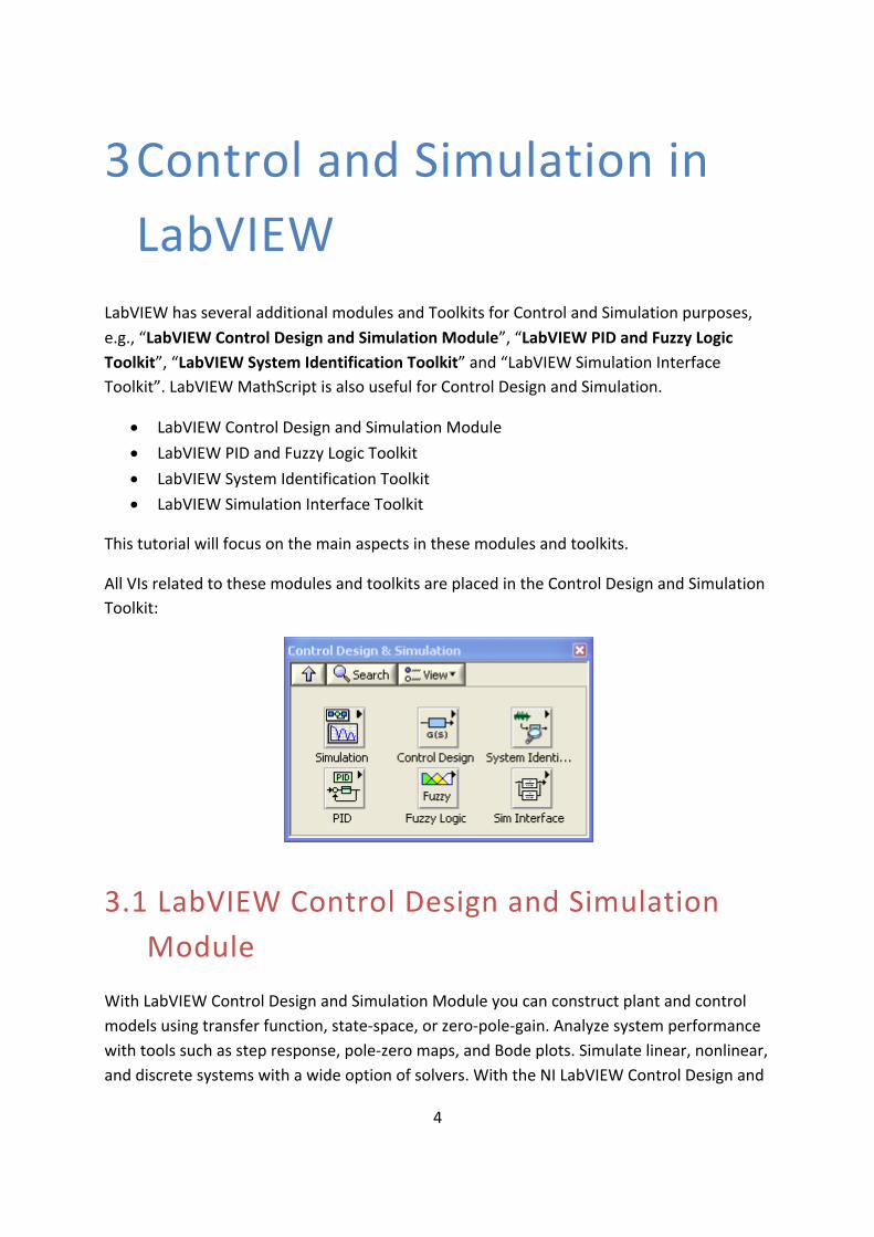
LabVIEWhasseveraladditionalmodulesandToolkitsforControlandSimulationpurposes,e.g.,“LabVIEWControlDesignandSimulationModule”,“LabVIEWPIDandFuzzyLogicToolkit”,“LabVIEWSystemIdentificationToolkit”and“LabVIEWSimulationInterfaceToolkit”.LabVIEWMathScriptisalsousefulforControlDesignandSimulation.

• LabVIEWControlDesignandSimulationModule• LabVIEWPIDandFuzzyLogicToolkit• LabVIEWSystemIdentificationToolkit• LabVIEWSimulationInterfaceToolkit

Thistutorialwillfocusonthemainaspectsinthesemodulesandtoolkits.

AllVIsrelatedtothesemodulesandtoolkitsareplacedintheControlDesignandSimulationToolkit:

3.1 LabVIEWControlDesignandSimulationModule

WithLabVIEWControlDesignandSimulationModuleyoucanconstructplantandcontrolmodelsusingtransferfunction,state-space,orzero-pole-gain.Analyzesystemperformancewithtoolssuchasstepresponse,pole-zeromaps,andBodeplots.Simulatelinear,nonlinear,anddiscretesystemswithawideoptionofsolvers.WiththeNILabVIEWControlDesignand



SimulationModule,youcananalyzeopen-loopmodelbehavior,designclosed-loopcontrollers,simulateonlineandofflinesystems,andconductphysicalimplementations.

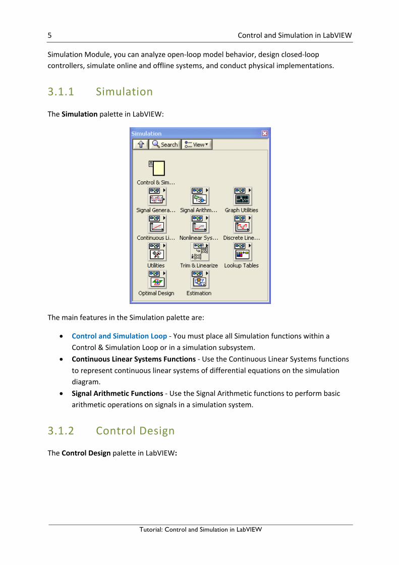
3.1.1 Simulation

TheSimulationpaletteinLabVIEW:

ThemainfeaturesintheSimulationpaletteare:

• ControlandSimulationLoop-YoumustplaceallSimulationfunctionswithinaControl&SimulationLooporinasimulationsubsystem.

• ContinuousLinearSystemsFunctions-UsetheContinuousLinearSystemsfunctionstorepresentcontinuouslinearsystemsofdifferentialequationsonthesimulationdiagram.

• SignalArithmeticFunctions-UsetheSignalArithmeticfunctionstoperformbasicarithmeticoperationsonsignalsinasimulationsystem.

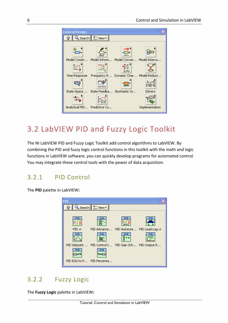
3.1.2 ControlDesign

TheControlDesignpaletteinLabVIEW:



3.2 LabVIEWPIDandFuzzyLogicToolkitTheNILabVIEWPIDandFuzzyLogicToolkitaddcontrolalgorithmstoLabVIEW.BycombiningthePIDandfuzzylogiccontrolfunctionsinthistoolkitwiththemathandlogicfunctionsinLabVIEWsoftware,youcanquicklydevelopprogramsforautomatedcontrol.Youmayintegratethesecontroltoolswiththepowerofdataacquisition.

3.2.1 PIDControl

ThePIDpaletteinLabVIEW:

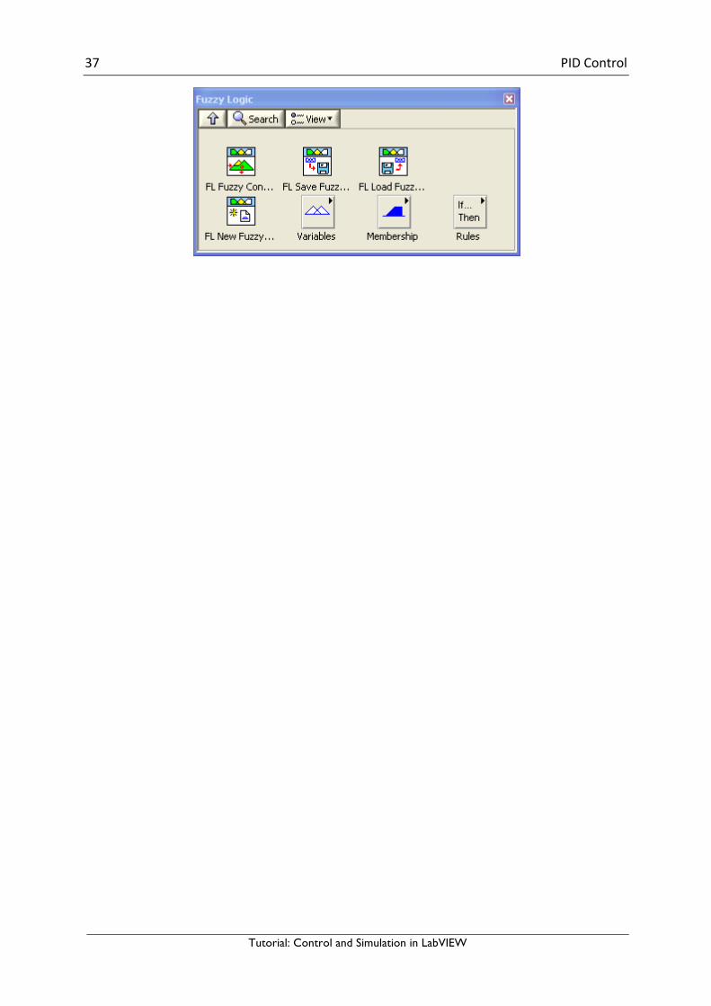
3.2.2 FuzzyLogic

TheFuzzyLogicpaletteinLabVIEW:



3.3 LabVIEWSystemIdentificationToolkitThe“LabVIEWSystemIdentificationToolkit”combinesdataacquisitiontoolswithsystemidentificationalgorithmsforplantmodeling.YoucanusetheLabVIEWSystemIdentificationToolkittofindempiricalmodelsfromrealplantstimulus-responseinformation.

TheSystemIdentificationpaletteinLabVIEW:

8

4 SimulationSimulationisaprocessthatinvolvesusingsoftwaretorecreateandanalyzethebehaviorofdynamicsystems.Youusethesimulationprocesstolowerproductdevelopmentcostsbyacceleratingproductdevelopment.Youalsousethesimulationprocesstoprovideinsightintothebehaviorofdynamicsystemsyoucannotreplicateconvenientlyinthelaboratory.Forexample,simulatingajetenginesavestime,labor,andmoneycomparedtobuilding,testing,andrebuildinganactualjetengine.YoucanusetheLabVIEWControlDesignandSimulationModuletosimulateadynamicsystemoracomponentofadynamicsystem.Forexample,youcansimulateonlytheplantwhileusinghardwareforthecontroller,actuators,andsensors(Hardware-in-the-loopSimulation).

Adynamicsystemmodelisadifferentialordifferenceequationthatdescribesthebehaviorofthedynamicsystem.

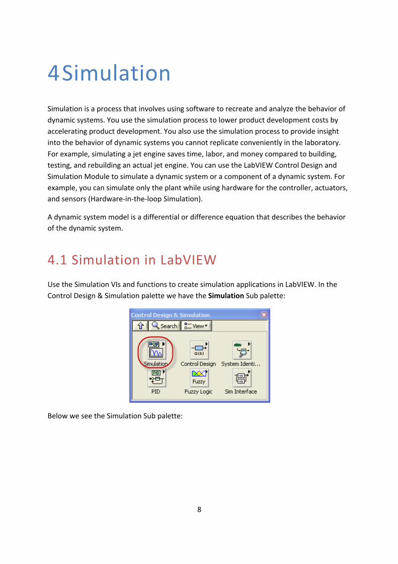
4.1 SimulationinLabVIEWUsetheSimulationVIsandfunctionstocreatesimulationapplicationsinLabVIEW.IntheControlDesign&SimulationpalettewehavetheSimulationSubpalette:

BelowweseetheSimulationSubpalette:

9 Simulation


Note!Allthe“Blocks”intheSimulationpalettearenotSubVIs,i.e.,wecannotdouble-clickonthemandopentheBlockDiagrambecausetheyhavenone.AlltheBlocksintheSimulationpalettemustbeusedinsidetheControlandSimulationLoop(explainedbelow).

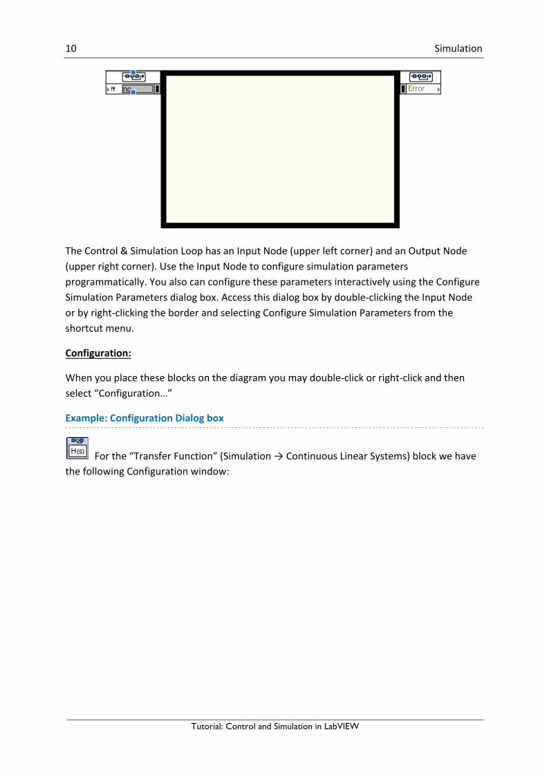
ControlandSimulationLoop:

Inthe“Simulation”Subpalettewehavethe“ControlandSimulationLoop”whichisveryusefulinsimulations:

YoumustplaceallSimulationfunctionswithinaControl&SimulationLooporinasimulationsubsystem.YoualsocanplacesimulationsubsystemswithinaControl&SimulationLooporanothersimulationsubsystem,oryoucanplacesimulationsubsystemsonablockdiagramoutsideaControl&SimulationLooporrunthesimulationsubsystemsasstand-aloneVIs.

10 Simulation


TheControl&SimulationLoophasanInputNode(upperleftcorner)andanOutputNode(upperrightcorner).UsetheInputNodetoconfiguresimulationparametersprogrammatically.YoualsocanconfiguretheseparametersinteractivelyusingtheConfigureSimulationParametersdialogbox.Accessthisdialogboxbydouble-clickingtheInputNodeorbyright-clickingtheborderandselectingConfigureSimulationParametersfromtheshortcutmenu.

Configuration:

Whenyouplacetheseblocksonthediagramyoumaydouble-clickorright-clickandthenselect“Configuration…”

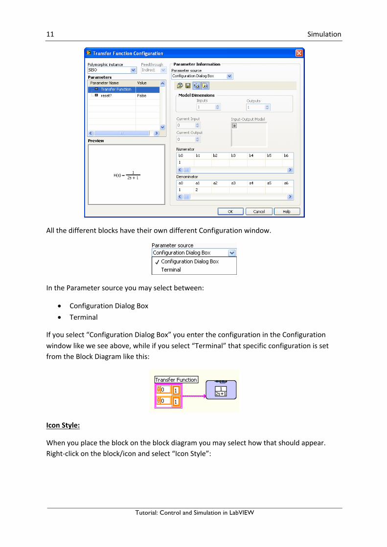
Example:ConfigurationDialogbox

Forthe“TransferFunction”(Simulation→ContinuousLinearSystems)blockwehavethefollowingConfigurationwindow:

11 Simulation


AllthedifferentblockshavetheirowndifferentConfigurationwindow.

IntheParametersourceyoumayselectbetween:

• ConfigurationDialogBox• Terminal

Ifyouselect“ConfigurationDialogBox”youentertheconfigurationintheConfigurationwindowlikeweseeabove,whileifyouselect“Terminal”thatspecificconfigurationissetfromtheBlockDiagramlikethis:

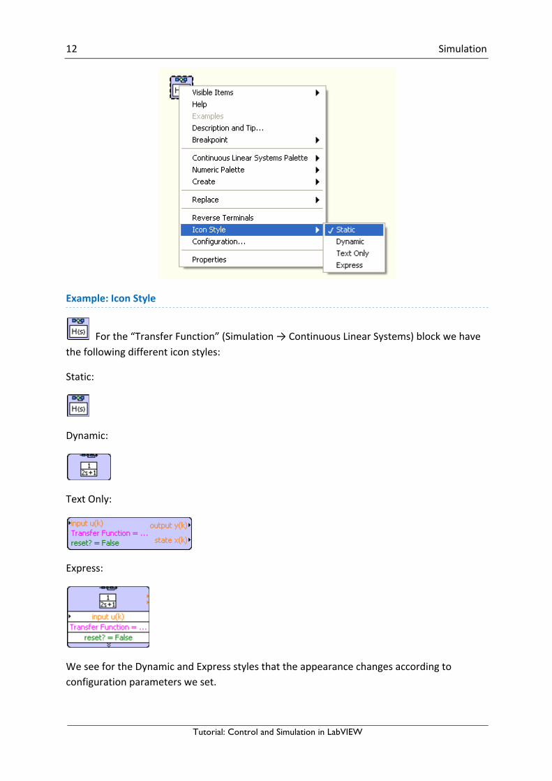
IconStyle:

Whenyouplacetheblockontheblockdiagramyoumayselecthowthatshouldappear.Right-clickontheblock/iconandselect“IconStyle”:

12 Simulation


Example:IconStyle

Forthe“TransferFunction”(Simulation→ContinuousLinearSystems)blockwehavethefollowingdifferenticonstyles:

Static:

Dynamic:

TextOnly:

Express:

WeseefortheDynamicandExpressstylesthattheappearancechangesaccordingtoconfigurationparametersweset.

13 Simulation


Ipersonallypreferthe“static”iconstylebecauseitdoesnotrequirelotsofspaceonthediagram.

4.2 SimulationSubsystemYoumaycreateaSimulationSubsystem(File→New…):

TheSimulationSubsystemisveryusefulwhendealingwithlargersimulationsystemsinordertocreateamorestructuredcode.Irecommendthatyou(always)usethisfeature.

TheSimulationSubsystemisalmostequaltoanormalLabVIEWBlockDiagrambutnoticethebackgroundcolorisslightlydarker.

Note!InordertoopentheSimulationSubsystem,right-clickandselect“OpenSubsystem”.

TheSimulationSubsystemmayalsoberepresentedbydifferenticons.Ifyouselect“dynamic”iconstyle,youwillseea“miniature”versionofthesubsystemlikethis:

14 Simulation


Youmaydraginthecornerinordertoincreaseordecreasethedynamicicon.

Ifyouselect“static”iconstyleyouseetheiconyoucreatedwiththeIconEditor.

Likethis:

4.3 ContinuousLinearSystemsInthe“ContinuousLinearSystems”Subpalettewewanttocreateasimulationmodel:

ThemostusedblocksprobablyareIntegrator,TransportDelay,State-SpaceandTransferFunction.

15 Simulation


Whenyouplacetheseblocksonthediagramyoumaydouble-clickorright-clickandthenselect“Configuration…”

Integrator-Integratesacontinuousinputsignalusingtheordinarydifferentialequation(ODE)solveryouspecifyforthesimulation.

TheConfigurationwindowfortheIntegratorblocklookslikethis:

TransportDelay-Delaystheinputsignalbytheamountoftimeyouspecify.

TheConfigurationwindowfortheTransportDelayblocklookslikethis:

TransferFunction-Implementsasystemmodelintransferfunctionform.YoudefinethesystemmodelbyspecifyingtheNumeratorandDenominatorofthetransferfunctionequation.

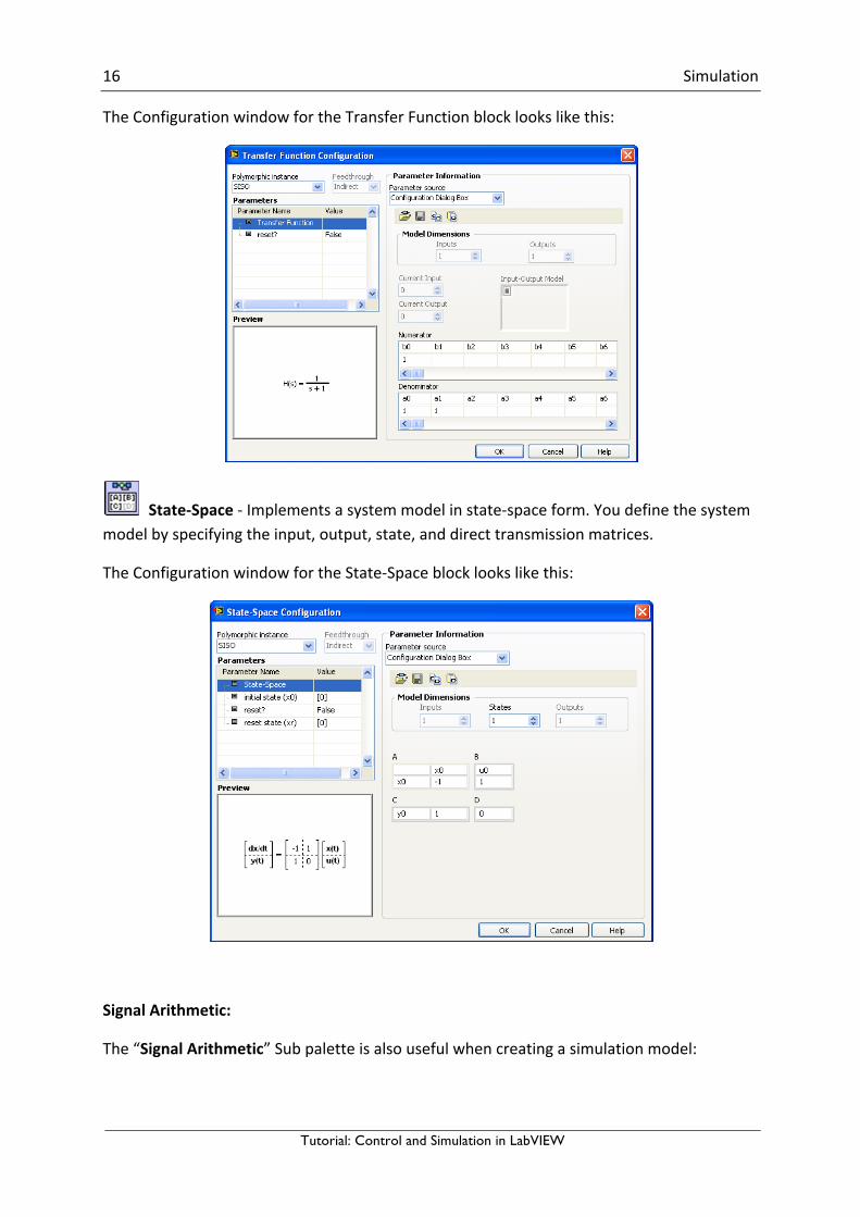
16 Simulation


TheConfigurationwindowfortheTransferFunctionblocklookslikethis:

State-Space-Implementsasystemmodelinstate-spaceform.Youdefinethesystemmodelbyspecifyingtheinput,output,state,anddirecttransmissionmatrices.

TheConfigurationwindowfortheState-Spaceblocklookslikethis:

SignalArithmetic:

The“SignalArithmetic”Subpaletteisalsousefulwhencreatingasimulationmodel:

17 Simulation


Example:SimulationModel

BelowweseeanexampleofasimulationmodelcreatedinLabVIEW.

Example:Simulation

BelowweseeanexampleofasimulationmodelusingtheControlandSimulationLoop.

Noticethefollowing:

18 Simulation


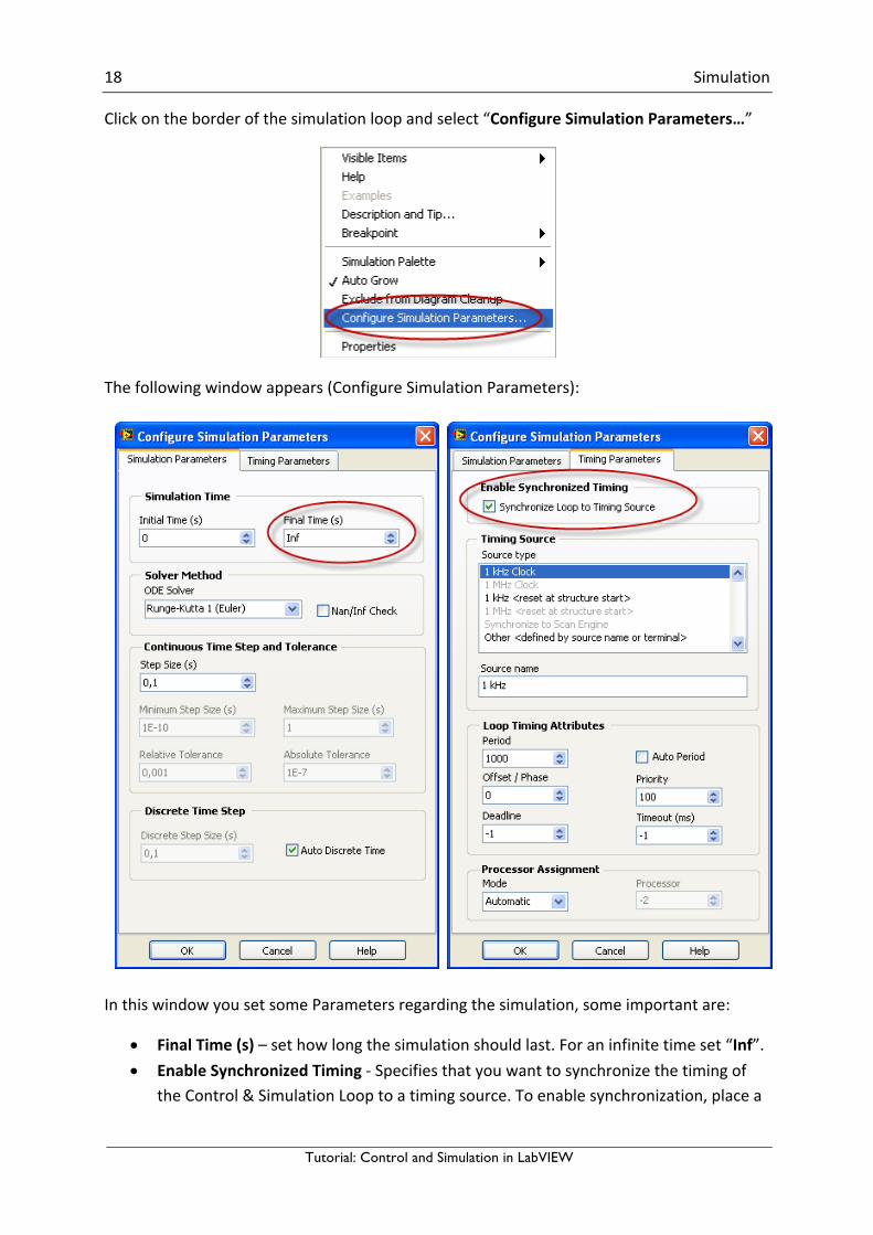
Clickontheborderofthesimulationloopandselect“ConfigureSimulationParameters…”

Thefollowingwindowappears(ConfigureSimulationParameters):

InthiswindowyousetsomeParametersregardingthesimulation,someimportantare:

• FinalTime(s)–sethowlongthesimulationshouldlast.Foraninfinitetimeset“Inf”.• EnableSynchronizedTiming-Specifiesthatyouwanttosynchronizethetimingof

theControl&SimulationLooptoatimingsource.Toenablesynchronization,placea

19 Simulation


checkmarkinthischeckboxandthenchooseatimingsourcefromtheSourcetypelistbox.

ClicktheHelpbuttonformoredetails.

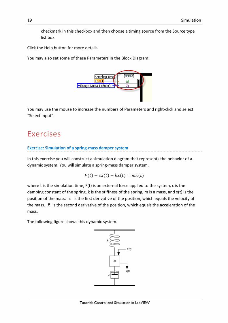
YoumayalsosetsomeoftheseParametersintheBlockDiagram:

YoumayusethemousetoincreasethenumbersofParametersandright-clickandselect“SelectInput”.

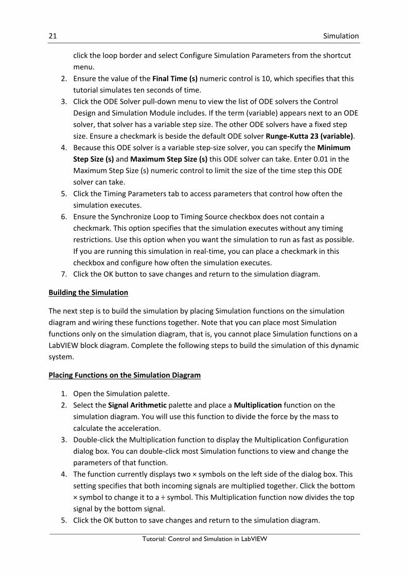
ExercisesExercise:Simulationofaspring-massdampersystem

Inthisexerciseyouwillconstructasimulationdiagramthatrepresentsthebehaviorofadynamicsystem.Youwillsimulateaspring-massdampersystem.

𝐹(𝑡) − 𝑐𝑥(𝑡) − 𝑘𝑥(𝑡) = 𝑚𝑥(𝑡)

wheretisthesimulationtime,F(t)isanexternalforceappliedtothesystem,cisthedampingconstantofthespring,kisthestiffnessofthespring,misamass,andx(t)isthepositionofthemass. 𝑥 isthefirstderivativeoftheposition,whichequalsthevelocityofthemass. 𝑥 isthesecondderivativeoftheposition,whichequalstheaccelerationofthemass.

Thefollowingfigureshowsthisdynamicsystem.

20 Simulation


Thegoalistoviewthepositionx(t)ofthemassmwithrespecttotimet.Youcancalculatethepositionbyintegratingthevelocityofthemass.Youcancalculatethevelocitybyintegratingtheaccelerationofthemass.Ifyouknowtheforceandmass,youcancalculatethisaccelerationbyusingNewton'sSecondLawofMotion,givenbythefollowingequation:

Force=Mass×Acceleration

Therefore,

Acceleration=Force/Mass

Substitutingtermsfromthedifferentialequationaboveyieldsthefollowingequation:

𝑥 =1𝑚(𝐹 − 𝑐𝑥 − 𝑘𝑥)

Youwillconstructasimulationdiagramthatiteratesthefollowingstepsoveraperiodoftime.

CreatingtheSimulationDiagram

YoucreateasimulationdiagrambyplacingaControl&SimulationLoopontheLabVIEWblockdiagram.

1. LaunchLabVIEWandselectFile»NewVItocreateanew,blankVI. 2. SelectWindow»ShowBlockDiagramtoviewtheblockdiagram.Youalsocanpress

the<Ctrl-E>keystoviewtheblockdiagram. 3. IfyouarenotalreadyviewingtheFunctionspalette,selectView»FunctionsPaletteto

displaythispalette. 4. SelectControlDesign&Simulation»SimulationtoviewtheSimulationpalette. 5. ClicktheControl&SimulationLoopicon. 6. Movethecursorovertheblockdiagram.Clicktoplacethetopleftcorneroftheloop,

dragthecursordiagonallytoestablishthesizeoftheloop,andclickagaintoplacetheloopontheblockdiagram.

ThesimulationdiagramistheareaenclosedbytheControl&SimulationLoop.Noticethesimulationdiagramhasapaleyellowbackgroundtodistinguishitfromtherestoftheblockdiagram.YoucanresizetheControl&SimulationLoopbydraggingitsborders.

ConfiguringSimulationParameters

TheControl&SimulationLoopcontainstheparametersthatdefinehowthesimulationexecutes.Completethefollowingstepstoviewandconfigurethesesimulationparameters.

1. Double-clicktheInputNode,attachedtotheleftsideoftheControl&SimulationLoop,todisplaytheConfigureSimulationParametersdialogbox.Youalsocanright-

21 Simulation


clicktheloopborderandselectConfigureSimulationParametersfromtheshortcutmenu.

2. EnsurethevalueoftheFinalTime(s)numericcontrolis10,whichspecifiesthatthistutorialsimulatestensecondsoftime.

3. ClicktheODESolverpull-downmenutoviewthelistofODEsolverstheControlDesignandSimulationModuleincludes.Iftheterm(variable)appearsnexttoanODEsolver,thatsolverhasavariablestepsize.TheotherODEsolvershaveafixedstepsize.EnsureacheckmarkisbesidethedefaultODEsolverRunge-Kutta23(variable).

4. BecausethisODEsolverisavariablestep-sizesolver,youcanspecifytheMinimumStepSize(s)andMaximumStepSize(s)thisODEsolvercantake.Enter0.01intheMaximumStepSize(s)numericcontroltolimitthesizeofthetimestepthisODEsolvercantake.

5. ClicktheTimingParameterstabtoaccessparametersthatcontrolhowoftenthesimulationexecutes.

6. EnsuretheSynchronizeLooptoTimingSourcecheckboxdoesnotcontainacheckmark.Thisoptionspecifiesthatthesimulationexecuteswithoutanytimingrestrictions.Usethisoptionwhenyouwantthesimulationtorunasfastaspossible.Ifyouarerunningthissimulationinreal-time,youcanplaceacheckmarkinthischeckboxandconfigurehowoftenthesimulationexecutes.

7. ClicktheOKbuttontosavechangesandreturntothesimulationdiagram.

BuildingtheSimulation

ThenextstepistobuildthesimulationbyplacingSimulationfunctionsonthesimulationdiagramandwiringthesefunctionstogether.NotethatyoucanplacemostSimulationfunctionsonlyonthesimulationdiagram,thatis,youcannotplaceSimulationfunctionsonaLabVIEWblockdiagram.Completethefollowingstepstobuildthesimulationofthisdynamicsystem.

PlacingFunctionsontheSimulationDiagram

1. OpentheSimulationpalette. 2. SelecttheSignalArithmeticpaletteandplaceaMultiplicationfunctiononthe

simulationdiagram.Youwillusethisfunctiontodividetheforcebythemasstocalculatetheacceleration.

3. Double-clicktheMultiplicationfunctiontodisplaytheMultiplicationConfigurationdialogbox.Youcandouble-clickmostSimulationfunctionstoviewandchangetheparametersofthatfunction.

4. Thefunctioncurrentlydisplaystwo×symbolsontheleftsideofthedialogbox.Thissettingspecifiesthatbothincomingsignalsaremultipliedtogether.Clickthebottom×symboltochangeittoa÷symbol.ThisMultiplicationfunctionnowdividesthetopsignalbythebottomsignal.

5. ClicktheOKbuttontosavechangesandreturntothesimulationdiagram.

22 Simulation


6. Right-clicktheMultiplicationfunctionandselectVisibleItems»Labelfromtheshortcutmenu.Double-clicktheMultiplicationlabelandenterCalculateAccelerationasthenewlabel.

7. ReturntotheSimulationpaletteandselecttheContinuousLinearSystemspalette. 8. PlaceanIntegratorfunctiononthesimulationdiagram.Youwillusethisfunctionto

calculatevelocitybyintegratingacceleration. 9. LabelthisIntegratorfunctionCalculateVelocity. 10. Pressthe<Ctrl>keyandclickanddragtheIntegratorfunctiontoanotherlocationon

thesimulationdiagram.ThisactioncreatesacopyoftheIntegratorfunction,whichyouwillusetocalculatepositionbyintegratingvelocity.LabelthisnewIntegratorfunctionCalculatePosition.

11. SelecttheGraphUtilitiespaletteandplacetwoSimTimeWaveformfunctionsonthesimulationdiagram.Youwillusethesefunctionstoviewtheresultsofthesimulationovertime.

12. EachSimTimeWaveformfunctionhasanassociatedWaveformChart.LabelthefirstwaveformchartVelocityandthesecondwaveformchartPosition.

13. Arrangethefunctionstolooklikethefollowingsimulationdiagram. 14. SavethisVIbyselectingFile»Save.SavethisVItoaconvenientlocationas“Spring-

MassDamperExample.vi”.

TheBlockDiagramshouldnowlooklikethis:

WiringtheSimulationFunctionsTogether

Thenextstepiswiringthefunctionstogethertorepresenttheflowofdatafromonefunctiontoanother.

Note!Wiresonthesimulationdiagramincludearrowsthatshowthedirectionofthedataflow,whereaswiresonaLabVIEWblockdiagramdonotshowthesearrows.

23 Simulation


Completethefollowingstepstowirethesefunctionstogether.

1. Right-clicktheOperand1inputoftheCalculateAccelerationfunctionandselectCreate»Controlfromtheshortcutmenutoaddanumericcontroltothefrontpanelwindow.

2. LabelthiscontrolForce. 3. Double-clickthiscontrolonthesimulationdiagram.LabVIEWdisplaysthefrontpanel

andhighlightstheForcecontrol. 4. DisplaytheblockdiagramandcreateacontrolfortheOperand2inputofthe

CalculateAccelerationfunction.LabelthisnewcontrolMass. 5. WiretheResultoutputoftheCalculateAccelerationfunctiontotheinputinputof

theCalculateVelocityfunction. 6. WiretheoutputoutputoftheCalculateVelocityfunctiontotheinputinputofthe

CalculatePositionfunction. 7. Right-clickthewireyoujustcreatedandselectCreateWireBranchfromtheshortcut

menu.WirethisbranchtotheValueinputoftheSimTimeWaveformfunctionthathastheVelocitywaveformchart.

8. WiretheoutputoutputoftheCalculatePositionfunctiontotheValueinputoftheSimTimeWaveformfunctionthathasthePositionwaveformchart.


RunningtheSimulation

YounowcanrunthissimulationtotestthatthedataisflowingproperlythroughtheSimulationfunctions.Completethefollowingstepstorunthissimulation.

24 Simulation


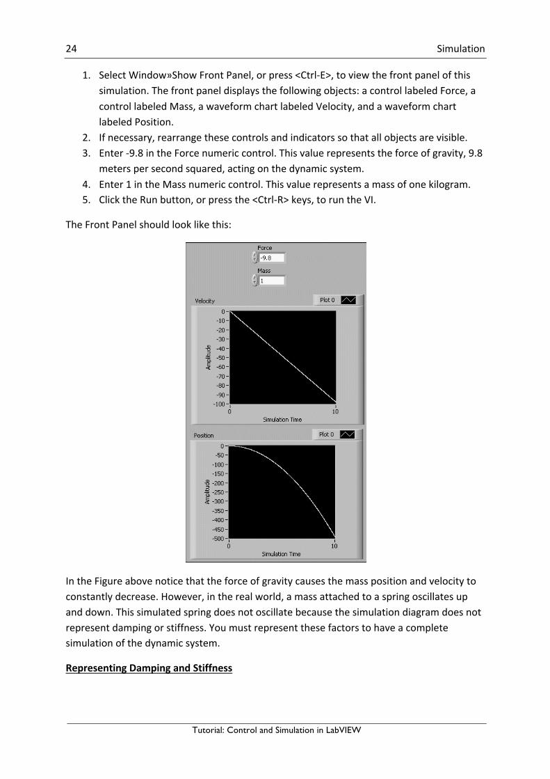
1. SelectWindow»ShowFrontPanel,orpress<Ctrl-E>,toviewthefrontpanelofthissimulation.Thefrontpaneldisplaysthefollowingobjects:acontrollabeledForce,acontrollabeledMass,awaveformchartlabeledVelocity,andawaveformchartlabeledPosition.

2. Ifnecessary,rearrangethesecontrolsandindicatorssothatallobjectsarevisible. 3. Enter-9.8intheForcenumericcontrol.Thisvaluerepresentstheforceofgravity,9.8

meterspersecondsquared,actingonthedynamicsystem. 4. Enter1intheMassnumericcontrol.Thisvaluerepresentsamassofonekilogram. 5. ClicktheRunbutton,orpressthe<Ctrl-R>keys,toruntheVI.

TheFrontPanelshouldlooklikethis:

IntheFigureabovenoticethattheforceofgravitycausesthemasspositionandvelocitytoconstantlydecrease.However,intherealworld,amassattachedtoaspringoscillatesupanddown.Thissimulatedspringdoesnotoscillatebecausethesimulationdiagramdoesnotrepresentdampingorstiffness.Youmustrepresentthesefactorstohaveacompletesimulationofthedynamicsystem.

RepresentingDampingandStiffness

25 Simulation


Representingdampingandstiffnessinvolvesfeedingbackthevelocityandposition,eachmultipliedbyadifferentconstant,totheinputoftheCalculateAccelerationfunction.RecallthefollowingdifferentialequationthisVIsimulates.

𝐹(𝑡) − 𝑐𝑥(𝑡) − 𝑘𝑥(𝑡) = 𝑚𝑥(𝑡)

Inthepreviousequation,noticeyoumultiplythedampingconstantcbythevelocityofthemass 𝑥.Youmultiplythestiffnessconstantkbythemasspositionx(t).Youthensubtractthesequantitiesfromtheexternalforceappliedtothemass.

Completethefollowingstepstorepresentdampingandstiffnessinthisdynamicsystemmodel.

1. Viewthesimulationdiagram. 2. SelecttheSignalArithmeticpaletteandplaceaSummationfunctiononthe

simulationdiagram.MovethisfunctiontotheleftoftheForceandMasscontrols. 3. Double-clicktheSummationfunctiontoconfigureitsoperation.Bydefault,the

Summationfunctiondisplaysthefollowingthreeinputterminals:aØsymbol,a+symbol,anda–symbol.Thisconfigurationsubtractsoneinputsignalfromanother.

4. ClicktheØsymboltwicetochangethisterminaltothe–symbol.ThisSummationfunctionnowsubtractsthetopandbottominputsignalsfromtheleftinputsignal.

5. ClicktheOKbuttontosavechangesandreturntothesimulationdiagram. 6. SelecttheSignalArithmeticpaletteandplaceaGainfunctiononthesimulation

diagram.MovethisfunctionabovetheexistingsimulationdiagramcodebutstillwithintheControl&SimulationLoop.

7. TheinputoftheGainfunctionisontheleftsideofthefunction,andtheoutputisontherightside.Youcanreversethedirectionoftheseterminalstoindicatefeedbackbetter.Right-clicktheGainfunctionandselectReverseTerminalsfromtheshortcutmenu.TheGainfunctionnowpointstowardtheleftsideofthesimulationdiagram.

8. LabelthisGainfunctionDamping. 9. Pressthe<Ctrl>keyanddragtheGainfunctiontocreateaseparatecopy.Movethis

copybelowtheexistingsimulationdiagramcodebutstillwithintheControl&SimulationLoop.LabelthisfunctionStiffness.

10. Right-clickthewireconnectingtheForcecontroltotheCalculateAccelerationfunctionandselectDeleteWireBranchfromtheshortcutmenu.MovetheForcecontroltotheleftoftheSummationfunction,andwirethiscontroltotheOperand2inputoftheSummationfunction.

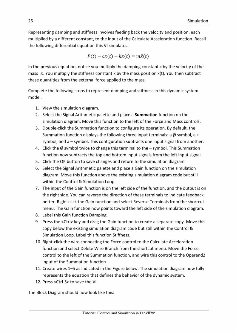
11. Createwires1–5asindicatedintheFigurebelow.Thesimulationdiagramnowfullyrepresentstheequationthatdefinesthebehaviorofthedynamicsystem.

12. Press<Ctrl-S>tosavetheVI.


26 Simulation


ConfiguringtheStiffnessoftheSpring

Beforeyourunthesimulationagain,youmustconfigurethestiffnessofthesimulatedspring.CompletethefollowingstepstoconfigurethisSimulationfunction.

1. Double-clicktheStiffnessfunctiontodisplaytheGainConfigurationdialogbox. 2. Enter100inthegainnumericcontrol.Thisvaluerepresentsastiffnessof100

Newtonspermeter. 3. ClickOKtoreturntothesimulationdiagram.NoticethattheStiffnessfunction

displays100. 4. DisplaythefrontpanelandensuretheForcecontrolissetto-9.8andtheMass

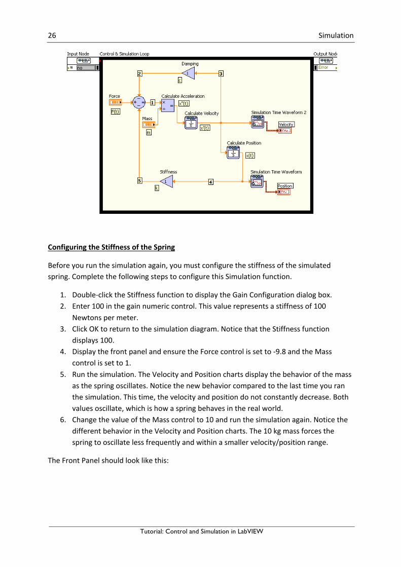
controlissetto1. 5. Runthesimulation.TheVelocityandPositionchartsdisplaythebehaviorofthemass

asthespringoscillates.Noticethenewbehaviorcomparedtothelasttimeyouranthesimulation.Thistime,thevelocityandpositiondonotconstantlydecrease.Bothvaluesoscillate,whichishowaspringbehavesintherealworld.

6. ChangethevalueoftheMasscontrolto10andrunthesimulationagain.NoticethedifferentbehaviorintheVelocityandPositioncharts.The10kgmassforcesthespringtooscillatelessfrequentlyandwithinasmallervelocity/positionrange.

TheFrontPanelshouldlooklikethis:

27 Simulation


ConfiguringSimulationFunctionsProgrammatically

TheprevioussectionprovidedinformationaboutconfiguringSimulationfunctionsusingtheconfigurationdialogbox.Insteadofusingtheconfigurationdialogbox,youcanimprovetheinteractivityofasimulationbycreatingfrontpanelcontrolsthatconfigureaSimulationfunctionprogrammatically.CompletethefollowingstepstoconfiguretheStiffnessfunctionprogrammatically.

1. IfyouarenotalreadyviewingtheContextHelpwindow,press<Ctrl-H>todisplaythiswindow.

2. DisplaytheblockdiagramandmovethecursorovertheStiffnessfunction.Noticethisfunctionhasonlyoneinputterminal.

3. DisplaytheGainConfigurationdialogboxoftheStiffnessfunction. 4. SelectTerminalfromtheParametersourcepull-downmenu.Thisactiondisablesthe

gainnumericcontrol. 5. ClicktheOKbuttontosavechangesandreturntotheblockdiagram. 6. MovethecursorovertheStiffnessfunction.NoticetheContextHelpwindowdisplays

theGainfunctionwiththenewgaininputterminal. 7. Createacontrolforthisinput,andlabelthecontrolgain(k).

28 Simulation


8. Viewthefrontpanel.Noticethenewcontrolgain(k).Enteravalueof100forthiscontrolandrunthesimulation.NoticethebehaviorisexactlythesameaswhenyouusedtheconfigurationdialogboxtoconfiguretheStiffnessfunction.

ModularizingSimulationDiagramCode

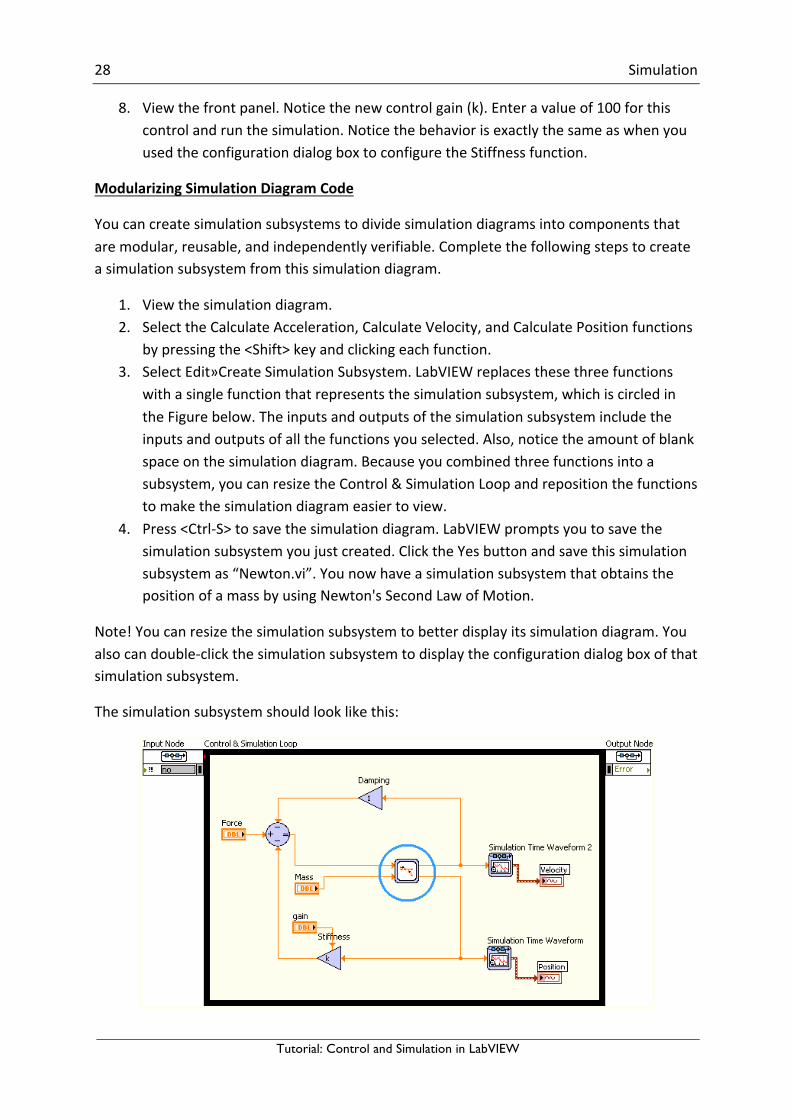
Youcancreatesimulationsubsystemstodividesimulationdiagramsintocomponentsthataremodular,reusable,andindependentlyverifiable.Completethefollowingstepstocreateasimulationsubsystemfromthissimulationdiagram.

1. Viewthesimulationdiagram. 2. SelecttheCalculateAcceleration,CalculateVelocity,andCalculatePositionfunctions

bypressingthe<Shift>keyandclickingeachfunction. 3. SelectEdit»CreateSimulationSubsystem.LabVIEWreplacesthesethreefunctions

withasinglefunctionthatrepresentsthesimulationsubsystem,whichiscircledintheFigurebelow.Theinputsandoutputsofthesimulationsubsystemincludetheinputsandoutputsofallthefunctionsyouselected.Also,noticetheamountofblankspaceonthesimulationdiagram.Becauseyoucombinedthreefunctionsintoasubsystem,youcanresizetheControl&SimulationLoopandrepositionthefunctionstomakethesimulationdiagrameasiertoview.

4. Press<Ctrl-S>tosavethesimulationdiagram.LabVIEWpromptsyoutosavethesimulationsubsystemyoujustcreated.ClicktheYesbuttonandsavethissimulationsubsystemas“Newton.vi”.YounowhaveasimulationsubsystemthatobtainsthepositionofamassbyusingNewton'sSecondLawofMotion.

Note!Youcanresizethesimulationsubsystemtobetterdisplayitssimulationdiagram.Youalsocandouble-clickthesimulationsubsystemtodisplaytheconfigurationdialogboxofthatsimulationsubsystem.

Thesimulationsubsystemshouldlooklikethis:

29 Simulation


EditingtheSimulationSubsystem

Editthesimulationsubsystem“Newton.vi”byright-clickingthissubsystemandselectingOpenSubsystemfromtheshortcutmenu.Viewthesimulationdiagram.

NoticethissimulationsubsystemdoesnotcontainaControl&SimulationLoop,buttheentirebackgroundispaleyellowtoindicateasimulationdiagram.IfyouplacethissimulationsubsysteminaControl&SimulationLoop,thesimulationsubsysteminheritsallsimulationparametersfromtheControl&SimulationLoop.

Ifyourunthissubsystemasastand-aloneVI,youcanconfigurethesimulationparametersbyselectingOperate»ConfigureSimulationParameters.AnyparametersyouconfigureusingthismethoddonottakeeffectwhenthesubsystemiswithinanotherControl&SimulationLoop.IfyouplacethissimulationsubsystemonablockdiagramoutsideaControl&SimulationLoop,youcanconfigurethesimulationparametersbydouble-clickingthesimulationsubsystemtodisplaytheconfigurationdialogboxofthatsimulationsubsystem.

ConfiguringSimulationParametersProgrammatically

Earlierinthisexercise,youusedtheConfigureSimulationParametersdialogboxtoconfiguretheparametersof“Spring-MassDamperExample.vi”.YoualsocanconfiguresimulationparametersprogrammaticallybyusingtheInputNodeoftheControl&SimulationLoop.Completethefollowingstepstoconfiguresimulationparametersprogrammatically.

1. Viewthesimulationdiagramof“Spring-MassDamperExample.vi”. 2. MovethecursorovertheInputNodetodisplayresizinghandles. 3. DragthebottomhandledowntodisplayallavailableNodeinputs.Youusethese

inputstoconfigurethesimulationparameterswithoutdisplayingtheConfigureSimulationParametersdialogbox.Youalsocanright-clicktheInputNodeandselectShowAllInputsfromtheshortcutmenu. Noticethegrayboxesnexttoeachinput.TheseboxesdisplayvaluesyouconfigureintheConfigureSimulationParametersdialogbox.Forexample,thethirdgrayboxfromthetopdisplays10.0000,whichisthevalueoftheFinalTimenumericcontrolthatyouconfigured.ThefifthgrayboxfromthetopdisplaysRK23.ThisboxspecifiesthecurrentODEsolver,whichyouconfiguredasRunge-Kutta23(variable).MovethecursorovertheleftedgeofeachNodeinputtodisplaythelabelofthatinput.

4. Right-clicktheinputterminaloftheODESolverinputandselectCreate»Constantfromtheshortcutmenu.AblockdiagramconstantappearsoutsidetheControl&SimulationLoop.ThevalueofthisconstantisRunge-Kutta1(Euler),whichisdifferentthanwhatyouconfiguredintheConfigureSimulationParametersdialogbox.However,thegrayboxdisappearsfromtheInputNode,indicatingthatthevalue

30 Simulation


ofthisparameterdoesnotcomefromtheConfigureSimulationParametersdialogbox.ValuesthatyouprogrammaticallyconfigureoverrideanysettingsyoumadeintheConfigureSimulationParametersdialogbox.

TheInputNodeshouldnowlooklikethefollowingfigure:

Summary

Thisexerciseintroducedyoutothefollowingconcepts:

Thesimulationdiagramreflectsthedynamicsystemmodelyouwanttosimulate.Thisdynamicsystemmodelisadifferentialordifferenceequationthatrepresentsadynamicsystem.

TheControl&SimulationLoopcontainstheparametersthatdefinethebehaviorofthesimulation.TheControl&SimulationLoopalsodefinesthevisualboundaryofthesimulationdiagram.Double-clicktheInputNodeoftheControl&SimulationLooptoaccessconfigurableparameters.YoualsocanexpandtheInputNodetoaccesstheseparameters.

TheSimulationpalettecontainstheVIsandfunctionsyouusetobuildasimulation.Youcandouble-clickmostSimulationfunctionstodisplayadialogboxthatconfiguresthatfunction.Youalsocancreateinputterminalsforfunctioninputs.

Youcancreatesimulationsubsystemstomodularize,encapsulate,validate,andre-useportionsofthesimulationdiagram.

31

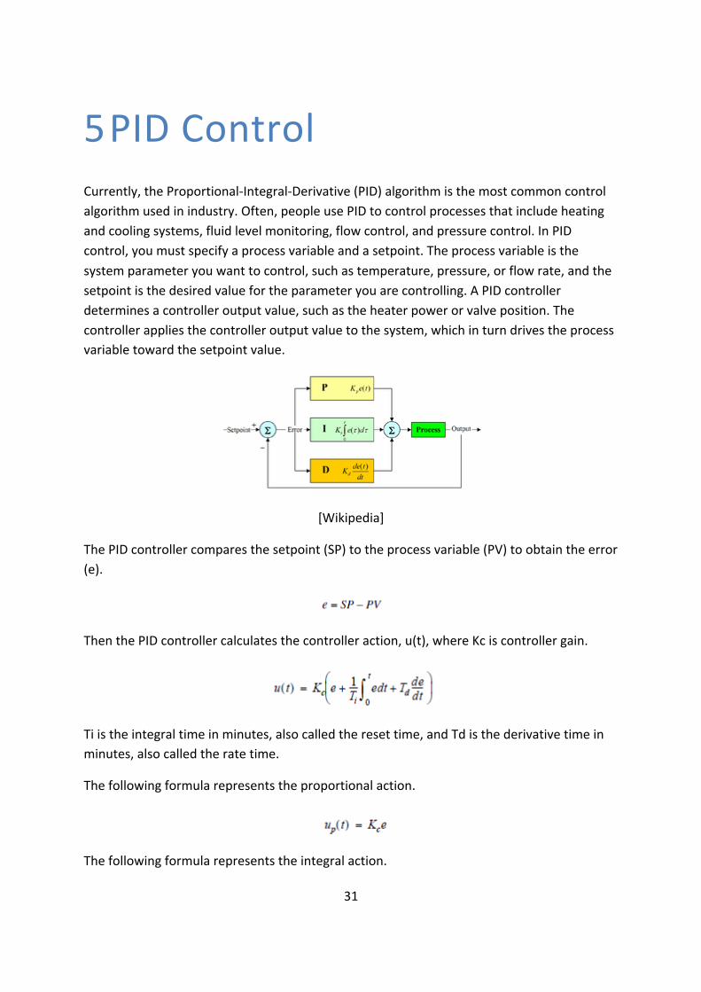
5 PIDControlCurrently,theProportional-Integral-Derivative(PID)algorithmisthemostcommoncontrolalgorithmusedinindustry.Often,peopleusePIDtocontrolprocessesthatincludeheatingandcoolingsystems,fluidlevelmonitoring,flowcontrol,andpressurecontrol.InPIDcontrol,youmustspecifyaprocessvariableandasetpoint.Theprocessvariableisthesystemparameteryouwanttocontrol,suchastemperature,pressure,orflowrate,andthesetpointisthedesiredvaluefortheparameteryouarecontrolling.APIDcontrollerdeterminesacontrolleroutputvalue,suchastheheaterpowerorvalveposition.Thecontrollerappliesthecontrolleroutputvaluetothesystem,whichinturndrivestheprocessvariabletowardthesetpointvalue.

[Wikipedia]

ThePIDcontrollercomparesthesetpoint(SP)totheprocessvariable(PV)toobtaintheerror(e).

ThenthePIDcontrollercalculatesthecontrolleraction,u(t),whereKciscontrollergain.

Tiistheintegraltimeinminutes,alsocalledtheresettime,andTdisthederivativetimeinminutes,alsocalledtheratetime.

Thefollowingformularepresentstheproportionalaction.

Thefollowingformularepresentstheintegralaction.

32 PIDControl


Thefollowingformularepresentsthederivativeaction.

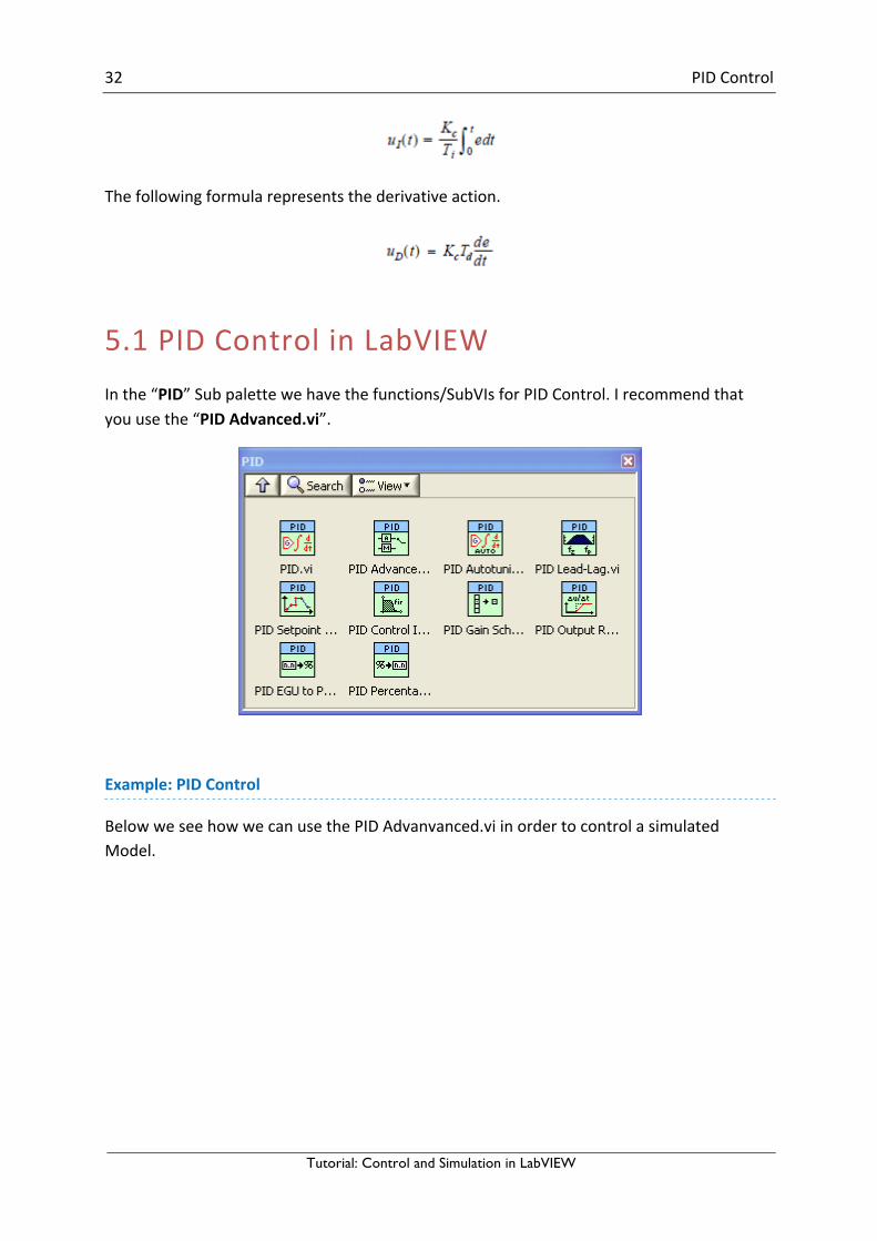
5.1 PIDControlinLabVIEWInthe“PID”Subpalettewehavethefunctions/SubVIsforPIDControl.Irecommendthatyouusethe“PIDAdvanced.vi”.

Example:PIDControl

BelowweseehowwecanusethePIDAdvanvanced.viinordertocontrolasimulatedModel.

33 PIDControl


5.2 Auto-tuningTheLabVIEWPIDandFuzzyLogicToolkitincludeaVIforauto-tuning.

34

6 ControlDesignControldesignisaprocessthatinvolvesdevelopingmathematicalmodelsthatdescribeaphysicalsystem,analyzingthemodelstolearnabouttheirdynamiccharacteristics,andcreatingacontrollertoachievecertaindynamiccharacteristics.

6.1 ControlDesigninLabVIEWControlDesignpalette:

35

7 SystemIdentification

7.1 SystemIdentificationinLabVIEWThe“SystemIdentificationToolkit”combinesdataacquisitiontoolswithsystemidentificationalgorithmsforaccurateplantmodeling.YoucantakeadvantageofLabVIEWintuitivedataacquisitiontoolssuchastheDAQAssistanttostimulateandacquiredatafromtheplantandthenautomaticallyidentifyadynamicsystemmodel.Youcanconvertsystemidentificationmodelstostate-space,transferfunction,orpole-zero-gainformforcontrolsystemanalysisanddesign.Thetoolkitincludesbuilt-infunctionsforcommontaskssuchasdatapreprocessing,modelcreation,andsystemanalysis.Usingotherbuilt-inutilities,youcanplotthemodelwithintuitivegraphicalrepresentationaswellasstorethemodel.

SystemIdentificationpalette:

36

8 FuzzyLogicFuzzylogicisamethodofrule-baseddecisionmakingusedforexpertsystemsandprocesscontrol.FuzzylogicdiffersfromtraditionalBooleanlogicinthatfuzzylogicallowsforpartialmembershipinaset.Youcanusefuzzylogictocontrolprocessesrepresentedbysubjective,linguisticdescriptions.

Afuzzysystemisasystemofvariablesthatareassociatedusingfuzzylogic.Afuzzycontrollerusesdefinedrulestocontrolafuzzysystembasedonthecurrentvaluesofinputvariables.

[Wikipedia]

8.1 FuzzyLogicinLabVIEWTheFuzzyLogicpaletteinLabVIEW:

37 PIDControl


38

9 LabVIEWMathScriptRequires:MathScriptRTModule

The“LabVIEWMathScriptWindow”isaninteractiveinterfaceinwhichyoucanenter.mfilescriptcommandsandseeimmediateresults,variablesandcommandshistory.Thewindowincludesacommand-lineinterfacewhereyoucanentercommandsone-by-oneforquickcalculations,scriptdebuggingorlearning.Alternatively,youcanenterandexecutegroupsofcommandsthroughascripteditorwindow.

Asyouwork,avariabledisplayupdatestoshowthegraphical/textualresultsandahistorywindowtracksyourcommands.Thehistoryviewfacilitatesalgorithmdevelopmentbyallowingyoutousetheclipboardtoreuseyourpreviouslyexecutedcommands.

Youcanusethe“LabVIEWMathScriptWindow”toentercommandsoneattime.Youalsocanenterbatchscriptsinasimpletexteditorwindow,loadedfromatextfile,orimportedfromaseparatetexteditor.The“LabVIEWMathScriptWindow”providesimmediatefeedbackinavarietyofforms,suchasgraphsandtext.

Example:

39 LabVIEWMathScript


9.1 HelpYoumayalsotypehelpinyourcommandwindow

>>help

Ormorespecific,e.g.,

>>help plot

9.2 ExamplesIadviseyoutotestalltheexamplesinthistextinLabVIEWMathScriptinordertogetfamiliarwiththeprogramanditssyntax.Allexamplesinthetextareoutlinedinaframelikethis:

>> …



ThisiscommandsyoushouldwriteintheCommandWindow.

YoutypeallyourcommandsintheCommandWindow.Iwillusethesymbol“>>”toillustratethatthecommandsshouldbewrittenintheCommandWindow.

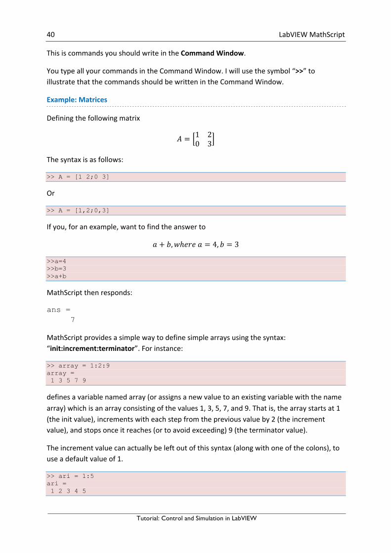
Example:Matrices

Definingthefollowingmatrix

𝐴 = 1 20 3

Thesyntaxisasfollows:

>> A = [1 2;0 3]

Or

>> A = [1,2;0,3]

Ifyou,foranexample,wanttofindtheanswerto

𝑎 + 𝑏,𝑤ℎ𝑒𝑟𝑒𝑎 = 4, 𝑏 = 3

>>a=4 >>b=3 >>a+b

MathScriptthenresponds:

ans = 7

MathScriptprovidesasimplewaytodefinesimplearraysusingthesyntax:“init:increment:terminator”.Forinstance:

>> array = 1:2:9 array = 1 3 5 7 9

definesavariablenamedarray(orassignsanewvaluetoanexistingvariablewiththenamearray)whichisanarrayconsistingofthevalues1,3,5,7,and9.Thatis,thearraystartsat1(theinitvalue),incrementswitheachstepfromthepreviousvalueby2(theincrementvalue),andstopsonceitreaches(ortoavoidexceeding)9(theterminatorvalue).

Theincrementvaluecanactuallybeleftoutofthissyntax(alongwithoneofthecolons),touseadefaultvalueof1.

>> ari = 1:5 ari = 1 2 3 4 5



assignstothevariablenamedarianarraywiththevalues1,2,3,4,and5,sincethedefaultvalueof1isusedastheincrementer.

Notethattheindexingisone-based,whichistheusualconventionformatricesinmathematics.Thisisatypicalforprogramminglanguages,whosearraysmoreoftenstartwithzero.

Matricescanbedefinedbyseparatingtheelementsofarowwithblankspaceorcommaandusingasemicolontoterminateeachrow.Thelistofelementsshouldbesurroundedbysquarebrackets:[].Parentheses:()areusedtoaccesselementsandsubarrays(theyarealsousedtodenoteafunctionargumentlist).

>> A = [16 3 2 13; 5 10 11 8; 9 6 7 12; 4 15 14 1] A = 16 3 2 13 5 10 11 8 9 6 7 12 4 15 14 1 >> A(2,3) ans = 11

Setsofindicescanbespecifiedbyexpressionssuchas"2:4",whichevaluatesto[2,3,4].Forexample,asubmatrixtakenfromrows2through4andcolumns3through4canbewrittenas:

>> A(2:4,3:4) ans = 11 8 7 12 14 1

Asquareidentitymatrixofsizencanbegeneratedusingthefunctioneye,andmatricesofanysizewithzerosoronescanbegeneratedwiththefunctionszerosandones,respectively.

>> eye(3) ans = 1 0 0 0 1 0 0 0 1 >> zeros(2,3) ans = 0 0 0 0 0 0 >> ones(2,3) ans = 1 1 1 1 1 1



9.3 UsefulcommandsHerearesomeusefulcommands:

Command Descriptioneye(x), eye(x,y) Identitymatrixoforderxones(x), ones(x,y) Amatrixwithonlyoneszeros(x), zeros(x,y) Amatrixwithonlyzerosdiag([x y z]) Diagonalmatrixsize(A) DimensionofmatrixAA’ InverseofmatrixA

9.4 PlottingThischapterexplainsthebasicconceptsofcreatingplotsinMathScript.

Topics:

• BasicPlotcommands

Example:Plotting

Functionplotcanbeusedtoproduceagraphfromtwovectorsxandy.Thecode:

x = 0:pi/100:2*pi; y = sin(x); plot(x,y)

43

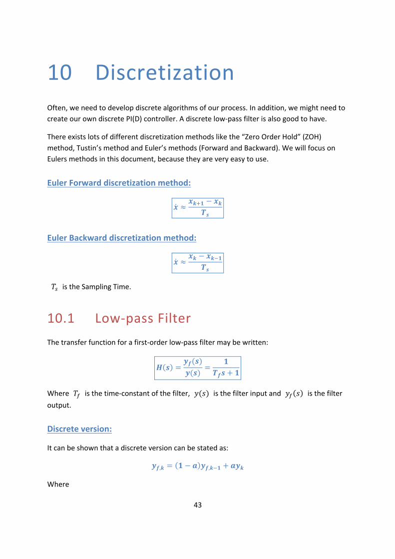
10 DiscretizationOften,weneedtodevelopdiscretealgorithmsofourprocess.Inaddition,wemightneedtocreateourowndiscretePI(D)controller.Adiscretelow-passfilterisalsogoodtohave.

Thereexistslotsofdifferentdiscretizationmethodslikethe“ZeroOrderHold”(ZOH)method,Tustin’smethodandEuler’smethods(ForwardandBackward).WewillfocusonEulersmethodsinthisdocument,becausetheyareveryeasytouse.

EulerForwarddiscretizationmethod:

𝒙 ≈𝒙𝒌=𝟏 − 𝒙𝒌

𝑻𝒔

EulerBackwarddiscretizationmethod:

𝒙 ≈𝒙𝒌 − 𝒙𝒌A𝟏

𝑻𝒔

𝑇C istheSamplingTime.

10.1 Low-passFilterThetransferfunctionforafirst-orderlow-passfiltermaybewritten:

𝑯 𝒔 =𝒚𝒇(𝒔)𝒚(𝒔)

=𝟏

𝑻𝒇𝒔 + 𝟏

Where 𝑇G isthetime-constantofthefilter, 𝑦(𝑠) isthefilterinputand 𝑦G 𝑠 isthefilteroutput.

Discreteversion:

Itcanbeshownthatadiscreteversioncanbestatedas:

𝒚𝒇,𝒌 = 𝟏 − 𝒂 𝒚𝒇,𝒌A𝟏 + 𝒂𝒚𝒌

Where

44 Discretization


𝒂 =𝑻𝒔

𝑻𝒇 + 𝑻𝒔

Where 𝑇C istheSamplingTime.

Itisagoldenrulethat 𝑇C ≪ 𝑇G andinpracticeweshouldusethefollowingrule:

𝑇C ≤𝑇G5

Example:

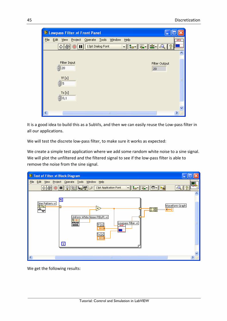
Wewillimplementthediscretelow-passfilteralgorithmbelowusingaFormulaNodeinLabVIEW:

𝑦G,N = 1 − 𝑎 𝑦G,NAO + 𝑎𝑦N

Where

𝑎 =𝑇C

𝑇G + 𝑇C

TheBlockDiagrambecomes:

TheFrontPanel:

45 Discretization


ItisagoodideatobuildthisasaSubVIs,andthenwecaneasilyreusetheLow-passfilterinallourapplications.

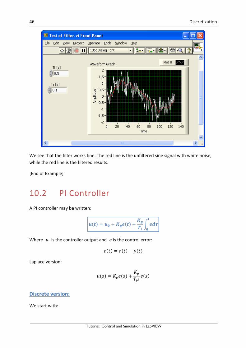
Wewilltestthediscretelow-passfilter,tomakesureitworksasexpected:

Wecreateasimpletestapplicationwhereweaddsomerandomwhitenoisetoasinesignal.Wewillplottheunfilteredandthefilteredsignaltoseeifthelow-passfilterisabletoremovethenoisefromthesinesignal.

Wegetthefollowingresults:

46 Discretization


Weseethatthefilterworksfine.Theredlineistheunfilteredsinesignalwithwhitenoise,whiletheredlineisthefilteredresults.

[EndofExample]

10.2 PIControllerAPIcontrollermaybewritten:

𝒖 𝒕 = 𝒖𝟎 + 𝑲𝒑𝒆 𝒕 +𝑲𝒑

𝑻𝒊𝒆𝒅𝝉𝒕

𝟎

Where 𝑢 isthecontrolleroutputand 𝑒isthecontrolerror:

𝑒 𝑡 = 𝑟 𝑡 − 𝑦(𝑡)

Laplaceversion:

𝑢 𝑠 = 𝐾[𝑒 𝑠 +𝐾[𝑇\𝑠

𝑒 𝑠

Discreteversion:

Westartwith:

47 Discretization


𝑢 𝑡 = 𝑢] + 𝐾[𝑒 𝑡 +𝐾[𝑇\

𝑒𝑑𝜏`

]

Inordertomakeadiscreteversionusing,e.g.,Euler,wecanderivebothsidesoftheequation:

𝑢 = 𝑢] + 𝐾[𝑒 +𝐾[𝑇\𝑒

IfweuseEulerForwardweget:

𝑢N − 𝑢NAO𝑇C

=𝑢],N − 𝑢],NAO

𝑇C+ 𝐾[

𝑒N − 𝑒NAO𝑇C

+𝐾[𝑇\𝑒N

Thenweget:

𝒖𝒌 = 𝒖𝒌A𝟏 + 𝒖𝟎,𝒌 − 𝒖𝟎,𝒌A𝟏 + 𝑲𝒑 𝒆𝒌 − 𝒆𝒌A𝟏 +𝑲𝒑

𝑻𝒊𝑻𝒔𝒆𝒌

Where

𝑒N = 𝑟N − 𝑦N

Wecanalsosplittheequationabovein2differentparsbysetting:

∆𝑢N = 𝑢N − 𝑢NAO

ThisgivesthefollowingPIcontrolalgorithm:

𝒆𝒌 = 𝒓𝒌 − 𝒚𝒌

∆𝒖𝒌 = 𝒖𝟎,𝒌 − 𝒖𝟎,𝒌A𝟏 + 𝑲𝒑 𝒆𝒌 − 𝒆𝒌A𝟏 +𝑲𝒑

𝑻𝒊𝑻𝒔𝒆𝒌

𝒖𝒌 = 𝒖𝒌A𝟏 + ∆𝒖𝒌

ThisalgorithmcaneasilybeimplementedinLabVIEWorotherlanguagessuchas,e.g.,C#orMATLAB.

FormoredetailsabouthowtoimplementthisinC#,seetheTutorial“DataAcquisitioninC#”,availablefromhttps://www.halvorsen.blog.

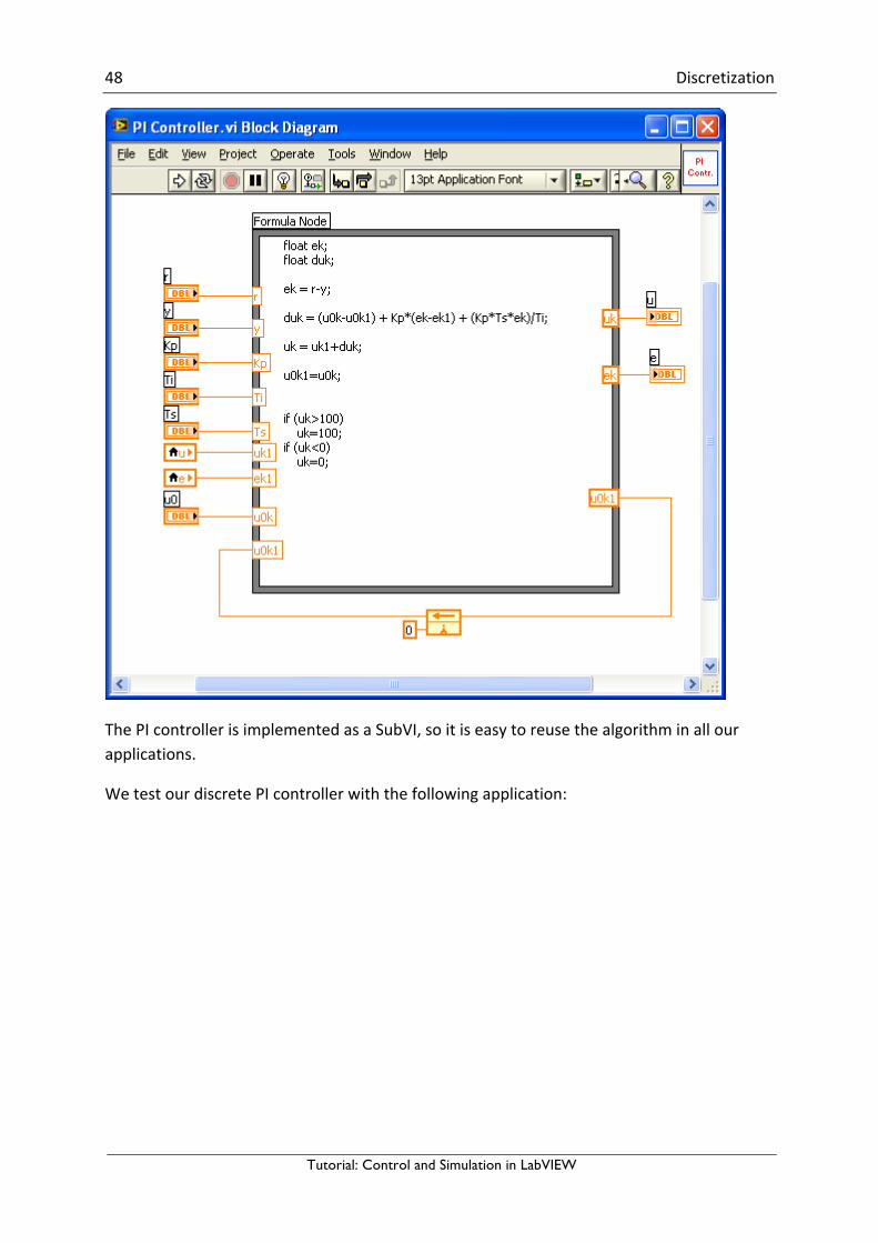
LabVIEWExample:

BelowwehaveimplementedthediscretePIcontrollerusingaFormulaNodeinLabVIEW:

48 Discretization


ThePIcontrollerisimplementedasaSubVI,soitiseasytoreusethealgorithminallourapplications.

WetestourdiscretePIcontrollerwiththefollowingapplication:

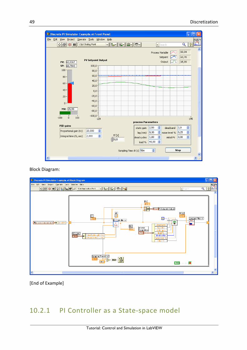
49 Discretization


BlockDiagram:

[EndofExample]

10.2.1 PIControllerasaState-spacemodel

50 Discretization


Weset 𝑧 = OC𝑒 ⇒ 𝑠𝑧 = 𝑒 ⇒ 𝑧 = 𝑒

Thisgives:

𝑧 = 𝑒

𝑢 = 𝐾[𝑒 +𝐾[𝑇\𝑧

Where

𝑒 = 𝑟 − 𝑦

Discreteversion:

UsingEuler:

𝑧 ≈𝑧N=O − 𝑧N

𝑇C


Thisgives:

𝑧N=O − 𝑧N𝑇C

= 𝑒N

𝑢N = 𝐾[𝑒N +𝐾[𝑇\𝑧N

Finally:

𝒆𝒌 = 𝒓𝒌 − 𝒚𝒌

𝒖𝒌 = 𝑲𝒑𝒆𝒌 +𝑲𝒑

𝑻𝒊𝒛𝒌

𝒛𝒌=𝟏 = 𝒛𝒌 + 𝑻𝒔𝒆𝒌

ThisalgorithmcaneasilybeimplementedinLabVIEWorotherlanguagessuchas,e.g.,C#orMATLAB.

FormoredetailsabouthowtoimplementthisinC#,seetheTutorial“DataAcquisitioninC#”,availablefromhttps://www.halvorsen.blog.

10.3 ProcessModel

51 Discretization


Wewilluseasimplewatertanktoillustratehowtocreateadiscreteversionofamathematicalprocessmodel.Belowweseeanillustration:

Averysimple(linear)modelofthewatertankisasfollows:

𝐴`ℎ = 𝐾[𝑢−𝐹fg`

or

ℎ =1𝐴`

𝐾[𝑢−𝐹fg`

Where:

• ℎ [cm]isthelevelinthewatertank• 𝑢 [V]isthepumpcontrolsignaltothepump• 𝐴` [cm2]isthecross-sectionalareainthetank• 𝐾[ [(cm3/s)/V]isthepumpgain• 𝐹fg` [cm3/s]istheoutflowthroughthevalve(thisoutflowcanbemodeledmore

accuratelytakingintoaccountthevalvecharacteristicexpressingtherelationbetweenpressuredropacrossthevalveandtheflowthroughthevalve).

WecanusetheEulerForwarddiscretizationmethodinordertocreateadiscretemodel:

𝑥 ≈𝑥N=O − 𝑥N

𝑇C

Thenweget:

ℎN=O − ℎN𝑇C

=1𝐴`

𝐾[𝑢N−𝐹fg`

52 Discretization


Finally:

𝒉𝒌=𝟏 = 𝒉𝒌 +𝑻𝒔𝑨𝒕

𝑲𝒑𝒖𝒌−𝑭𝒐𝒖𝒕

Thismodelcaneasilybeimplementedinacomputerusing,e.g.,MATLAB,LabVIEWorC#.

FormoredetailsforhowtodothisinC#,seetheTutorial“DataAcquisitioninC#”.

InLabVIEWthiscan,e.g.,beimplementedinaFormulaNodeorMathScriptNode.

Example:

InthisexamplewewillsimulateaBacteriaPopulation.

InthisexamplewewilluseLabVIEWandtheLabVIEWControlDesignandSimulationModuletosimulateasimplemodelofabacteriapopulationinajar.

Themodelisasfollows:

birthrate=bx

deathrate=px2

Thenthetotalrateofchangeofbacteriapopulationis:

𝑥 = 𝑏𝑥 − 𝑝𝑥w

Wesetb=1/hourandp=0.5bacteria-hourinourexample.

Wewillsimulatethenumberofbacteriainthejarafter1hour,assumingthatinitiallythereare100bacteriapresent.

WewillsimulatethesystemusingaForLoopinLabVIEWandimplementthediscretemodelinaFormulaNode.

Step1:Westartbycreatingthediscretemodel.

IfweuseEulerForwarddifferentiationmethod:


𝑇C


Weget:

𝑥N=O − 𝑥N𝑇C

= 𝑏𝑥N − 𝑝𝑥Nw

53 Discretization


Thisgives:

𝑥N=O = 𝑥N + 𝑇C(𝑏𝑥N − 𝑝𝑥Nw)

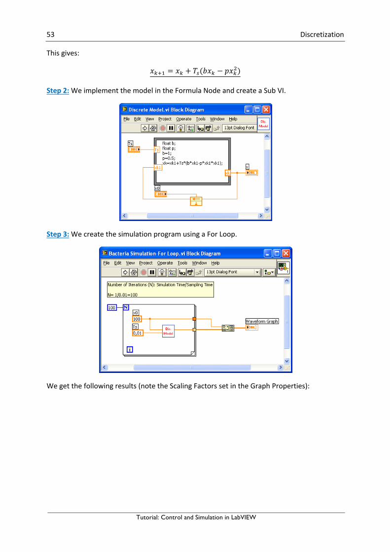
Step2:WeimplementthemodelintheFormulaNodeandcreateaSubVI.

Step3:WecreatethesimulationprogramusingaForLoop.

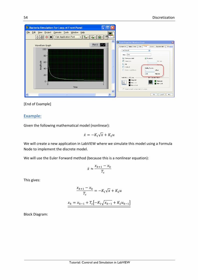
Wegetthefollowingresults(notetheScalingFactorssetintheGraphProperties):

54 Discretization


[EndofExample]

Example:

Giventhefollowingmathematicalmodel(nonlinear):

𝑥 = −𝐾O 𝑥 + 𝐾w𝑢

WewillcreateanewapplicationinLabVIEWwherewesimulatethismodelusingaFormulaNodetoimplementthediscretemodel.

WewillusetheEulerForwardmethod(becausethisisanonlinearequation):


𝑇C

Thisgives:

𝑥N=O − 𝑥N𝑇C

= −𝐾O 𝑥 + 𝐾w𝑢

𝑥N = 𝑥NAO + 𝑇C −𝐾O 𝑥NAO + 𝐾w𝑢NAO

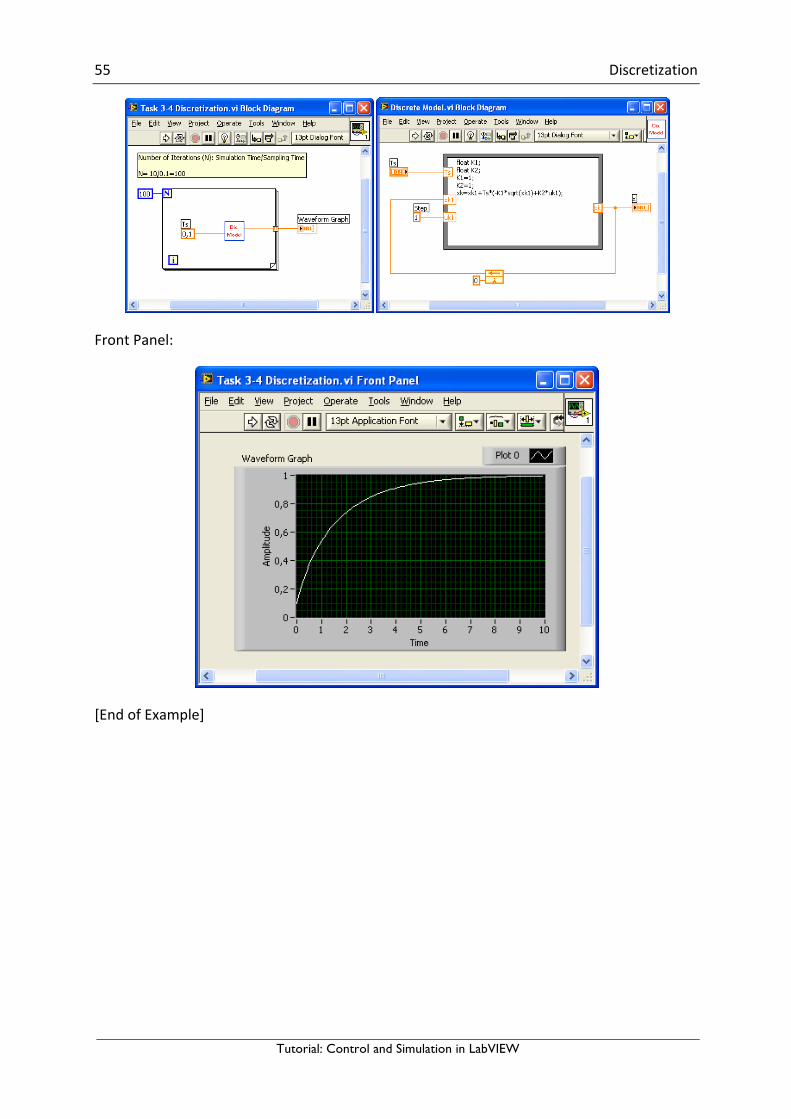
BlockDiagram:

55 Discretization


FrontPanel:

[EndofExample]

control and simulation in labview · tutorial: control and simulation in labview 3.2 labview pid...

Documents