control and protection of hvdc grids · particular friends within the medow projects for creating...
TRANSCRIPT
Control and Protection of HVDC Grids
i
Control and Protection of HVDC Grids
THESIS SUBMITTED FOR THE DEGREE OF
DOCTOR OF PHILOSOPHY
SHENG WANG
School of Engineering
Cardiff University
Cardiff, 2016

Control and Protection of HVDC Grids
ii
Declaration
This work has not been submitted in substance for any other degree or award at this or any
other university or place of learning, nor is being submitted concurrently in candidature for
any degree or other award.
Signed………………………………………… (candidate) Date……………………..
STATEMENT 1
This thesis is being submitted in partial fulfilment of the requirements for the degree of
……… (insert Mch, MD, MPhil, PhD etc, as appropriate)
Signed………………………………………… (candidate) Date……………………..
STATEMENT 2
This thesis is the result of my own independent work/investigation, except where otherwise
stated, and the thesis has not been edited by a third party beyond what is permitted by Cardiff
University’s Policy on the Use of Third Party Editors by Research Degree Students. Other
sources are acknowledged by explicit references. The views expressed are my own.
Signed………………………………………… (candidate) Date……………………..
STATEMENT 3
I hereby give consent for my thesis, if accepted, to be available online in the University’s
Open Access repository and for inter-library load, and for the title and summary to be made
available to outside organisations.
Signed………………………………………… (candidate) Date……………………..

Control and Protection of HVDC Grids
iii
Abstract
The decarbonisation of Europe’s energy sector is a key driver for the development of
integrated HVDC networks or DC grids. A multi-terminal HVDC grid will enable a more
reliable power transfer from offshore wind farms and will facilitate the cross-border exchange
of energy between different countries. However, the widespread deployment of DC grids is
prevented by technical challenges, including the control and protection of DC grids. In order
to close the gap, this thesis aims to contribute to three aspects (1): developing a control
method for DC grids operation; (2): developing a method for optimising wind power delivery
using DC grids; (3): developing a protection method for fast DC fault current interruption.
The control of a DC grid demands the regulation of DC voltage and hence keeps the
power into and out from the DC grid balanced. It is also important to keep the accuracy of
regulating the converter DC current. In this thesis, the Autonomous Converter Control (ACC)
is developed to meet this requirement. With this method, alternative droop control
characteristics can be used for individual converters to share the responsibility of regulation
of DC voltage while precisely controlling the converter DC current. The control algorithms of
alterative droop characteristics are developed and interactions of different control
characteristics are analysed. Furthermore, the potential risk of having multiple cross-over in
control characteristics is uncovered. The method for designing droop characteristics is
provided to avoid the multiple cross-over. The ACC is demonstrated on different simulation
platforms including the PSCAD/EMTDC and a real-time hardware 4-terminal HVDC test rig.
It is found that the proper use of alternative droop characteristics can achieve better current
control performance. The adverse impact of having multiple cross-over in control
characteristics is also studied using both simulation platforms.
The effect of the control of both converters and DC power flow controllers (DC-PFCs)
on DC power flow in steady state is also investigated. A method for re-dispatching control
orders to optimise the wind power delivery is developed. Case studies are undertaken and it is
found that both the DC line power loss and wind power curtailment can be reduced by re-
dispatching the control orders of converters and DC-PFCs.
The protection of a DC grid demands a very fast speed for fault current interruption.
Conventional methods proposed for HVDC grid protection take delays of several
milliseconds to discriminate a faulted circuit to healthy circuits and then allow the DC circuit
breakers (DC-CBs) to open at the faulted circuits. The fault current will keep rising during

Control and Protection of HVDC Grids
iv
the delayed time caused by fault discrimination. The Open Grid protection method is thus
developed to interrupt fault current before fault discrimination. With this method, multiple
DC-CBs open to interrupt the fault current based on local measurements of voltage (and
current) and the DC-CBs on healthy circuits will reclose to achieve discrimination afterwards.
This will reduce the delay for fault current interruption and hence the fault current can be
interrupted with a much smaller magnitude. The developed Open Grid method is tested via
simulation models developed in PSCAD/EMTDC. The results show that the Open Grid can
detect very quickly and discriminate various faults under different fault conditions in a
meshed HVDC grid.

Control and Protection of HVDC Grids
v
Acknowledgements
This dissertation would not have been possible without the invaluable and incessant
support that I receive from many generous people.
I would like to convey my deepest and most sincere gratitude to my supervisor, Dr. Jun
Liang, for delivering his extraordinary expertise, understanding and patience to shape my
Ph.D. career. I am profoundly indebted to Professor Nick Jenkins and Dr. Janaka Ekanayake
for their invaluable and ranging guidance on my research and inspiring support on improving
my language skills. I would like to give very special thanks to Dr. Carlos Ugalde-Loo for his
extremely kind encouragement and brilliant assistance throughout my study and every single
football game. My thanks go to Prof. Jianzhong Wu who supported me in many ways during
my studies in Cardiff. I also would like to thank Miss Catherine Roderick for sparing no
effort in helping me improve my presentation skills.
My heartfelt gratitude goes to our industrial colleagues and friends, Dr. Andrzej
Adamczyk, Mr. Robert Whitehouse and Prof. Carl Barker from Alstom Grid, for their kind
assistance and inputs from an industrial point of view.
I wish to express my gratitude to all my colleagues and friends who help me navigate
life as a Ph.D. student, especially those friends who shared the same office. I would like to
thank Mr. Rui Dantas and Mr Senthooran Balasubramaniam for misunderstanding all my
ideas, but nodding and smiling all the same. My thanks also go to colleagues at CIREGS, in
particular friends within the MEDOW projects for creating such a friendly environment. My
very special thanks go to Mr. Chuanyue Li who gave me much assistance in writing the thesis
after my developing severe dry eye. I would like to thank Dr. Oluwole Adeuyi who help me
proofread my thesis and provided kind comments.
I am particularly thankful to my family, especially my beloved parents for their
intellectual contributions to my academic nature. More importantly, I appreciate for their
unconditionally support, incessant encouragement and undoubted faith in my succeeding the
Ph.D. career throughout all these years.
Last but not the least, this dissertation contains the outcome of projects with financial
support from both Cardiff University and Alstom Grid. I would like to thank both.
Control and Protection of HVDC Grids
vi
Table of Contents
Declaration ..................................................................... ii
Abstract .......................................................................... iii
Acknowledgements ........................................................ v
Table of Contents ......................................................... vi
List of Tables ................................................................... x
List of Figures ................................................................ xi
List of abbreviations .................................................. xiv
Chapter 1 ......................................................................... 1
1. Introduction .......................................................... 1
1.1 UK Energy Policy............................... ............................................................. 1
1.2 Motivations for Developing HVDC Grids ....................................................... 2
1.2.1 Offshore Power Transmission............. ............................................................. 2
1.2.2 Point to Point HVDC Schemes........... ............................................................. 2
1.2.3 Towards HVDC Grids........................ .............................................................. 3
1.3 Technical Challenges.......................... ............................................................. 6
1.4 Research Objectives…………………… ......................................................... 8
1.5 Thesis Structure.................................. .............................................................. 9
1.6 List of Publications…………………… ......................................................... 10
1.7 Participation in Projects…………….. ........................................................... 12
Chapter 2 ...................................................................... 13
2. Technologies for HVDC Grids ........................ 13
2.1 Introduction………………………….. .......................................................... 13
2.2 AC/DC Converters…………………… ......................................................... 13

Control and Protection of HVDC Grids
vii
2.2.1 Line Commutated Converters……….. .......................................................... 13
2.2.2 Two-level Voltage Source Converters ........................................................... 14
2.2.3 Multi-level Modular Converters............. ........................................................ 15
2.2.4 Basic Control of MMCs........................... ...................................................... 16
2.3 HVDC Transmission Lines…………. .......................................................... 24
2.4 DC Circuit Breakers for HVDC Grid Protection ........................................... 27
2.4.1 HVDC Network Protection………….. .......................................................... 27
2.4.2 Proposed DC-CBs……………….………………………………………..….29
2.5 Summary…………………………….. .......................................................... 34
Chapter 3 ...................................................................... 35
3. Control of an HVDC Grid ................................ 35
3.1 Introduction…………………………. ........................................................... 35
3.2 HVDC Grid Control Review………….. ........................................................ 35
3.2.1 Requirement for Controlling an HVDC Grid ................................................. 35
3.2.2 Existing Control Methods…………….. ........................................................ 37
3.3 Autonomous Converter Control (ACC) ......................................................... 39
3.4 Control Algorithm……………………. ......................................................... 43
3.5 Interaction of Control Characteristics. ........................................................... 46
3.5.1 Interactions between Droop Characteristics ................................................... 46
3.5.2 Interactions of Power and Droop Characteristics ........................................... 47
3.5.3 Mathematical Analysis of control interactions ............................................... 49
3.6 Multiple Cross-Over of Control Characteristics ............................................ 52
3.7 Summary…………………………….. .......................................................... 56
Chapter 4 ...................................................................... 57
4. Computer Simulation and experimental Validation
of ACC ............................................................................ 57
4.1 Introduction……………………………. ....................................................... 57
Control and Protection of HVDC Grids
viii
4.2 Configuration of 4-terminal HVDC Test Rig ................................................ 57
4.3 System Configuration for Testing ACC ......................................................... 60
4.4 Control Units for Testing ACC…………… .................................................. 62
4.5 Implementation of Converter Control within ACC ........................................ 64
4.6 Case study…………………………….. ........................................................ 65
4.6.1 Coordination of Converter Control…………. ............................................... 65
4.6.2 Multiple Cross-overs in the Static Characteristics ......................................... 69
4.7 Summary……………………………. ........................................................... 73
Chapter 5 ...................................................................... 75
5. Optimisation of Wind Power Delivery using DC
Power Flow Controllers and AC/DC Converters75
5.1 Introduction…………………………….. ...................................................... 75
5.2 DC Power Flow Controllers……………….. ................................................. 75
5.3 Control Strategy of an HVDC Grid with DC-PFCs ....................................... 76
5.4 Control of DC-PFCs………………….. ......................................................... 77
5.5 DC Voltage versus Power Droop for Converters ........................................... 80
5.6 Impact of Changing Control Orders on DC Power Flow ............................... 81
5.7 Optimisation of DC Power Flow………. ....................................................... 84
5.8 Case study……………………………. ......................................................... 88
5.9 Summary……………………………… ........................................................ 93
Chapter 6 ...................................................................... 94
6. HVDC Grid Protection: Open Grid Method ... 94
6.1 Introduction…………………………. ........................................................... 94
6.2 DC Grid Protection Review………… ........................................................... 94
6.3 Basic Ideas of Open Grid Protection Approach ............................................. 96
6.4 Fault Detection Algorithm…………….. ....................................................... 97
6.5 Selection of Criteria for Fault Detection ........................................................ 98

Control and Protection of HVDC Grids
ix
6.6 Discrimination by Integration of Current in Transients ............................... 100
6.7 Discrimination by Residual Voltages …………………..………………….101
6.8 Simulation Results………………………. ................................................... 106
6.8.1 Test System…………………………. ......................................................... 106
6.8.2 Modelling of DC Components………… ..................................................... 106
6.8.3 Case Studies………………………… ......................................................... 109
6.8.4 Summary……………………………… ...................................................... 116
Chapter 7 .................................................................... 118
7. Conclusion and Future Work ....................... 118
7.1 Conclusion…………………………… ........................................................ 118
7.1.1 HVDC Grid Control…………………….. ................................................... 118
7.1.2 HVDC Grid Protection……………….. ....................................................... 120
7.2 Future Work………………………… ......................................................... 120
7.2.1 Protection of Non-permanent DC Fault ...................................................... 120
7.2.2 Protection of DC OHLs Sharing a Common Tower .................................... 121
References ................................................................. 122
Appendix A ................................................................... 134
Control and Protection of HVDC Grids
x
List of Tables
Table 1-1 LIST OF MULTI-TERMINAL HVDC (MTDC) SYSTEM PROJECTS ............................. 4
Table 2-1 SUMMARY OF THE OPERATION WITH CVB ALGORITHM ....................................... 23
Table 3-1 COMPARISON OF AN AC GRID AND A DC GRID [57] ............................................. 36
Table 3-2 TERMINOLOGIES FOR DIFFERENT DROOP TYPES ................................................... 42
Table 3-3 SIGNAL FLOWING INTO/OUT OF THE SELECTION BLOCK ........................................ 44
Table 3-4 CURRENT CONTROL PERFORMANCE OF DIFFERENT CONTROL METHODS ............... 48
Table 4-1 SUMMARY OF SIMULATION PARAMETERS ............................................................ 61
Table 4-2 BASIC DATA OF CONVERTER CONTROL FOR TEST ONE .......................................... 69
Table 4-3 BASIC DATA OF CONVERTER CONTROL FOR TEST TWO ......................................... 71
Table 5-1 PARAMETERS OF DC DEVICES .............................................................................. 89
Table 5-2 RESULTS OF CASE ONE ......................................................................................... 90
Table 5-3 CHANGE OF CONTROL ORDERS IN CASE TWO ........................................................ 91
Table 5-4 COMPARISON OF WIND POWER DELIVERY IN CASE TWO ....................................... 91
Table 5-5 CHANGE OF CONTROL ORDERS IN CASE THREE ..................................................... 92
Table 5-6 COMPARISON OF WIND POWER DELIVERY IN CASE THREE .................................... 92
Table 6-1 COMPARISON OF VOLTAGE PROFILE ................................................................... 103
Table 6-2 PARAMETER FOR THE CONDUCTOR AND THE GROUND WIRE ............................. 107
Table 6-3 CONDUCTOR DATA AND GROUND WIRE DATA OF OHL MODEL .......................... 107
Table 6-4 THRESHOLDS OF PROTECTION AND CONTROL SETTING OF VSCS ....................... 109
Control and Protection of HVDC Grids
xi
List of Figures
Fig 1.1 Generation and transmission capacity forecast [2] ................................................... 1
Fig 1.2 Dogger Bank connection overview [4] ..................................................................... 2
Fig 1.3 VSC based MTDC systems projects: (a) Nao’ao MTDC, (b): Zhoushan MTDC
Interconnection, (c): South-West Link [20], (d): Tres amigas superstation [21] ....................... 5
Fig 1.4 Challenges towards a large HVDC grid ................................................................... 7
Fig 2.1 Typical layout of a LCC ......................................................................................... 13
Fig 2.2 Architecture of a 2-level VSC ................................................................................ 14
Fig 2.3 Sinusoidal Pulse Width Modulation ....................................................................... 15
Fig 2.4 Architecture of a MMC and the output AC waveform ........................................... 16
Fig 2.5 Hierarchical control structure of an MMC ............................................................. 17
Fig 2.6 Outer control loop for non-islanded control mode ................................................. 18
Fig 2.7 Inner decoupled current control for non-islanded control mode ............................ 19
Fig 2.8 Generation of AC voltage reference with islanded control mode .......................... 20
Fig 2.9 Phase disposition modulation ................................................................................. 21
Fig 2.10 Phase shift modulation .......................................................................................... 21
Fig 2.11 Nearest level control ............................................................................................. 21
Fig 2.12 Control of CVB ..................................................................................................... 22
Fig 2.13 Circulating current suppression control ................................................................ 24
Fig 2.14 Mass-impregnated cables [47] .............................................................................. 26
Fig 2.15 Extruded cables ..................................................................................................... 26
Fig 2.16 Protection of a P2P HVDC link ............................................................................ 27
Fig 2.17 Protection of a HVDC grid ................................................................................... 28
Fig 2.18 A passive mechanical resonant breaker [50] ........................................................ 30
Fig 2.19 An active mechanical active resonant breaker [53] .............................................. 30
Fig 2.20 Full solid-state breaker [54] .................................................................................. 31
Fig 2.21 Hybrid HVDC circuit breaker [56] ....................................................................... 32
Fig 2.22 Working principle of a hybrid HVDC breaker ..................................................... 33
Fig 2.23 Process of fault current interruption ..................................................................... 33
Fig 3.1 Control methods for a HVDC network ................................................................... 37
Fig 3.2 Control structure of the Autonomous Converter Control ....................................... 39
Fig 3.3 DC converter droop characteristics ......................................................................... 40
Fig 3.4 Current error ........................................................................................................... 41

Control and Protection of HVDC Grids
xii
Fig 3.5 Droop characteristics with current error function ................................................... 41
Fig 3.6 Further modification on current error function ....................................................... 42
Fig 3.7 Alternative droop control system ............................................................................ 43
Fig 3.8 Power control system .............................................................................................. 46
Fig 3.9 Interaction of different droop characteristics in (a): active range; (b): transition
range; and (c) outside the transition range ............................................................................... 47
Fig 3.10 Interaction of droop characteristics and power control characteristics ................. 48
Fig 3.11 A HVDC grid of controls in both power and alternative droop control ............... 49
Fig 3.12 a) Multiple Operating Points, b) Reduced Power, c) Increased Power ................ 53
Fig 3.13 Multiple operating points ...................................................................................... 53
Fig 4.1 Configuration of the 4-terminal HVDC test rig ...................................................... 57
Fig 4.2 Physical model of VSCs (a): inside view of cabinet of VSCs; (b) PCBs ............... 58
Fig 4.3 Inside view of cabinet containing Unidrives .......................................................... 59
Fig 4.4 Cable representations: (a) DC cable model (b) Physical representations ............... 60
Fig 4.5 Star-connected VSC simulator: (a) Circuit diagram; (b) Simulator set-up............. 60
Fig 4.6 Simplified VSC converter model [77] .................................................................... 62
Fig 4.7 Control boards within the dSPACE control unit .................................................... 62
Fig 4.8 Example of dSPACE – ControlDesk ...................................................................... 63
Fig 4.9 Self-built Graphical User Interface ......................................................................... 64
Fig 4.10 Hierarchical structure of converter control implemented in the test rig ............... 65
Fig 4.11 Current error function simulation- (a): PSCAD result; (b): experimental result .. 66
Fig 4.12 Converter operation during change of power condition - (a): PSCAD result; (b):
experimental result ................................................................................................................... 68
Fig 4.13 (a) PSCAD: conventional droop characteristics (power ramp 0 MW to 1500 MW)
.................................................................................................................................................. 70
Fig 4.14 (a) HVDC test rig: conventional droop characteristics (power ramp 0 to 750 W)
.................................................................................................................................................. 72
Fig 5.1 Control strategy of a HVDC grid having DC-PFCs ............................................... 76
Fig 5.2 Thyristor based Controllable Voltage Source (CVS) ............................................. 77
Fig 5.3 IGBT based CVS .................................................................................................... 78
Fig 5.4 An alternative power flow controller ...................................................................... 78
Fig 5.5 Outer control loop for CVSs ................................................................................... 79
Fig 5.6 An example of (a): Variable Resistor (VR) and (b): its control loop ..................... 79
Fig 5.7 Converter with V/P droop: (a) control structure (b) V/P droop characteristics ...... 80

Control and Protection of HVDC Grids
xiii
Fig 5.8 An HVDC Grid integrated with m AC/DC converters and n DC-PFCs ................. 82
Fig 5.9 Flow chart of solving optimal DC power flow ....................................................... 87
Fig 5.10 A 9-terminal DC system with the integration of a DC-PFC ................................. 89
Fig 6.1 Action sequence of: (a) Open Grid protection method; (b) Conventional DC grid
protection method .................................................................................................................... 96
Fig 6.2 One line diagram of the two-VSC, two-branch DC system ................................... 97
Fig 6.3 Post-fault characteristics of voltage and current ..................................................... 98
Fig 6.4 A hybrid DC-CB ..................................................................................................... 99
Fig 6.5 Integration of current in transient flowing through faulted circuit ....................... 100
Fig 6.6 Integration of current in transient flowing through healthy circuit ...................... 100
Fig 6.7 Residual DC voltage after DC-CBs opening ....................................................... 102
Fig 6.8 Extracted DC component of residual DC voltage ................................................ 104
Fig 6.9 Flow chart of DC-CB acting in a fault event ........................................................ 105
Fig 6.10 One line diagram of meshed DC test system Power Component ....................... 106
Fig 6.11 Structure of the OHL tower ................................................................................ 108
Fig 6.12 Configuration of cable modelling in PSCAD/EMTDC ...................................... 108
Fig 6.13 Sign convention of current in both poles ............................................................ 109
Fig 6.14 Pole to pole fault on OHL12: (a) DC voltage; (b) DC current; (c) tripping
timings of DC-CB .................................................................................................................. 110
Fig 6.15 Integration of current transient and current derivatives at: (a) OHL12; (b) OHL23;
(c) OHL14 .............................................................................................................................. 111
Fig 6.16 DC voltages and their DC components at (a): OHL12; (b) OHL23; (c) OHL14112
Fig 6.17 Pole to pole fault on Cable34: (a) DC voltage; (b) DC current; (c) tripping
timings of DC-CBs ................................................................................................................ 113
Fig 6.18 Pole to ground fault on OHL12: (a) DC voltage; (b) DC current; (c) tripping
timings of DC-CBs ................................................................................................................ 114
Fig 6.19 Integration of current transient and current derivatives at: (a) OHL12; (b) OHL23;
(c) OHL14 .............................................................................................................................. 115
Fig 6.20 DC voltages and their DC components at (a): OHL12; (b) OHL23; (c) OHL14116

Control and Protection of HVDC Grids
xiv
List of abbreviations
AC Alternate Current
ACC Autonomous Converter Control
AC-CB AC Circuit Breaker
A/D Analogue/Digital
B2B Back To Back
CAN Controller Area Network
CVB Capacitor Voltage Balancing
CVS Controllable Voltage Source
DC Direct Current
DC-CB DC Circuit Breaker
DC-PFC DC Power Flow Controller
DSP Digital Signal Processor
d-q Direct-Quadrature
EU European Union
FFT Fast Fourier Transfer
GDC Grid Dispatch Centre
GS Grid Side
GUI Graphical User Interface
HB Half Bridge
HMI Human-Machine Interface
HVAC High Voltage Alternate Current
HVDC High Voltage Direct Current
IGBT Insulated Gate Bipolar Transistor
I/O Input/Output
LCC Line Commutated Converter
LCS Load Commutation Switch
LRSP Load Reference Set Point
MFC Microsoft Foundation Class
MI Mass Impregnated
MMC Modular Multi-Level Converter
MOV Metal Oxide Varistor

Control and Protection of HVDC Grids
xv
MTDC Multi-terminal High Voltage Direct Current
NLC Nearest Level Control
NSCOGI North Sea Countries Offshore Grid Initiative
ODIS Offshore Development Information Statement
OFGEM Office for Gas and Electricity Markets
OHL Overhead Line
OP Operating Point
OPF Optimal Power Flow
P2P Point To Point
PCB Printed Circuit Boards
PD-PWM Phase Disposition Modulation
PI Proportional Integral
PLL Phase Locked Loop
PS-PWM Phase Shift Modulation
PWM Pulse Width Modulation
RCB Residual Circuit Breaker
SM Submodules
STATCOM Static Synchronous Compensator
STW Scottish Territorial Water
TSO Transmission System Operator
UFD Ultrafast Disconnector
UK United Kingdom
VR Variable Resistor
VSC Voltage Source Converter
WF Wind Farm

Control and Protection of HVDC Grids
1
Chapter 1
1. Introduction
1.1 UK ENERGY POLICY
The UK government anticipates that 15% of energy demand will be provided by
renewable sources and Green House Gas emissions will be reduced by 34% by 2020 and
eventually reduced by 80% by 2050. The National Grid Electricity Transmission has thus
proposed four different scenarios [1] with only the ‘Gone Green’ scenario [2] representing a
balanced approach to meeting this target in which electricity generation, heat and transport all
contribute.
Under the ‘Gone Green’ scenario conventional coal plants will gradually be replaced by
renewable energy generation. There will be 31% of electricity generated from renewable
sources by 2020 (See Fig 1.1). The total transmission connected wind capacity will reach 26
GW by 2020 in which offshore wind will have a high proportion (17 GW). The Crown Estate
has already issued three rounds of offshore wind farm licenses, which will potentially lead to
a total capacity of over 40 GW. The first two rounds (including Round 2 extension) will
contribute an offshore wind capacity of around 8 GW by 2020. The Round 3 and Scottish
Territorial Water (STW) projects will contribute the remaining 9 GW by 2020. The UK
government and OFGEM have estimated that the UK offshore transmission will spend over
15 billion pounds to connect the projects of the three rounds [3].
Fig 1.1 Generation and transmission capacity forecast [2]

Control and Protection of HVDC Grids
2
1.2 MOTIVATIONS FOR DEVELOPING HVDC GRIDS
1.2.1 OFFSHORE POWER TRANSMISSION
The average distance of the offshore WFs to shore will increase from 6 km in Round 1
projects to 65 km in Round 2 projects. For the Round 3 project on Dogger Bank, the average
distance will be about 197.2 km (See Fig 1.2). Submarine HVAC is not an economic solution
for transmitting power over such a long distance. HVAC transmission using cables is limited
by the generation of reactive power (which requires compensation by shunt reactors) and by
voltage. In contrast, HVDC transmission is free of reactive power and DC cables have higher
power rating than that of AC. DC converters offer extra flexibility for power and voltage
control, they can also support additional damping in case of power oscillations in AC grid.
HVDC is expected to be the predominant option for long distance offshore transmission.
Fig 1.2 Dogger Bank connection overview [4]
1.2.2 POINT TO POINT HVDC SCHEMES
Most of the existing HVDC transmission systems are point to point (P2P) schemes and
which are based on two technologies namely Line Commutated Converter (LCC-HVDC) or
Voltage Source Converter (VSC-HVDC). To date, LCC technology dominates the DC
transmission market. However, there are several limitations of LCC-HVDC which makes it

Control and Protection of HVDC Grids
3
inadequate for offshore transmission. The operation of a LCC requires voltage sources for
commutation. Harmonics generated by LCC converters needs the deployment of large filters
at converter stations. Commutation failure may occur in a LCC during system disturbance.
The reverse of power flow direction in LCC-HVDC system can only be achieved by
reversing voltage polarity.
Conversely, the operation of VSC converters does not consume reactive power while
the size of filters can be reduced (or avoided if MMC technology used) which leads to small
footprint of offshore platform. Both active and reactive power can be controlled in VSC-
HVDC and there is no commutation failure problem. Furthermore, VSC-HVDC systems can
reverse power flow direction by changing the direction of current which enables the wind
farm black-start. These benefits of VSC have driven the market of VSC transmission in
recent years; proposed VSC-HVDC schemes include Borwin, Dolwin, Helwin and Sylwin
projects.
1.2.3 TOWARDS HVDC GRIDS
It has been claimed that compared to several P2P systems, a HVDC grid has overall
lower conversion losses and lower cost by reducing the number of converter stations and
cable length. Interest in developing DC grids is reflected by the increased studies in which
HVDC grids are proposed. Examples are given below:
The “TradeWind” project [5] of Intelligent Energy Europe is the first EU-level study to
explore the benefits of building a European grid that can have on the integration of large
amounts of wind power. This was followed by the “OffshoreGrid” project [6] which provides
the first in-depth analysis of building a cost-efficient grid in the North and Baltic Seas. Both
studies show that a HVDC mesh grid would be economically optimum means of the
integration of offshore wind power. In 2009 to 2012, the countries around the North Sea
discussed building the North Sea Super Grid (NSSG) under the North Sea Countries Offshore
Grid Initiative (NSCOGI) [7]. Meanwhile, the UK National Grid proposed a coordinated
strategy for offshore transmission based on DC grid in the offshore development information
statement (ODIS) [8]. In 2013, the third demonstration project of “TWENTIES” [9] (funded
by European Commission’s Directorate-General for Energy) provided and demonstrated the
secure operation of key building blocks for designing future DC grids including voltage
source converter (VSC) and DC circuit breaker (DC-CB). The “MEDOW” project [10]
(funded by the People programme of the Seventh Framework Programme of the European

Control and Protection of HVDC Grids
4
Union) started in the same year and focuses on the research of using MTDC system to
integrate offshore wind power. The Friends of the Super Grid proposed the Roadmap to the
Supergrid Technologies [11] which anticipates a “DC supergrid” to be the backbone of
Europe’s future power system. This DC supergrid will deliver decarbonised electricity across
the continent and enhance the existing AC networks. The ENTSO-E also considers a DC
supergrid as one approach to meet the energy target for 2050 and it works in line with the
Agency for the Cooperation of Energy Regulators to draft the network code on HVDC
Connections [12]. Moreover, the working group B4 of CIGRE conducts a range of studies
which focus on the feasibility of HVDC grids [13], Grid Codes for HVDC grids [14], HVDC
grids modelling [15], load flow control device and system voltage control [16], control and
protection of HVDC grids [17] and optimal reliability and availability of HVDC grids [18].
To date, there are a few multi-terminal HVDC system projects as listed in Table 1-1.
Table 1-1 LIST OF MULTI-TERMINAL HVDC (MTDC) SYSTEM PROJECTS
Names/
Connection
No. of
Terminals
Converter
Type Rating Year
HVDC Italy–
Corsica–Sardinia 3 LCC 220kV/200MW 1987
Quebec – New
England
Transmission
5 (3 in operation) LCC ±450kV/2250MW 1992
Nelson River
HVDC System
2 (can be in
MTDC mode) LCC ±500kV/3800MW 1985
Pacific DC Intertie 2 (can be in
MTDC mode) LCC ±500kV/3100MW 1989
North-East Agra 4 LCC ±800kV/6000MW 2016 (Planed)
Shin Shinano3
terminal VSC-B2B 3 VSC 10.6kV/53MW 1999
Nao’ao MTDC 3 (4th terminal
being planed) VSC
±160 kV,
200/100/50MW 2013
Zhoushan MTDC
Interconnection 5 VSC
±200kV,100/100
/100/300/400MW 2014
Tres amigas
superstation 3 VSC ±345kV/750MW 2015
South-West Link 3 VSC ±300kV/1440MW 2018 (Planed)
Zhangjiakou DC
grid Demo Project 4 VSC ±500kV/3000MW 2018

Control and Protection of HVDC Grids
5
The first two commissioned MTDC systems (i.e. the connection between Italy, Corsica
and Sardinia and the connection from Hydro-Quebec to New England) are all LCC based and
have three terminals in operation. There are also LCC based bipolar HVDC schemes (i.e.
Nelson River HVDC System and Pacific DC Intertie) that are able to operate in a multi-
terminal mode. Another LCC-HVDC grid will be built in India. This 1,728 km-long HVDC
link will operate with an ultra-high DC voltage (i.e. ±800kV) and be able to deliver 6000MW
of hydroelectric power from the country’s northeast region to the city of Agra.
However, it appears that future DC grids for offshore transmission will be based on
VSC due to its superiority over LCC. The first VSC based MTDC system is the Shin Shinano
3 terminal VSC Back-to-Back (B2B) system which was commissioned in Shin Shinano
substation in Japan, 1999 [19]. This system interconnects the country’s two main power grid
sections which operate with different frequencies (i.e. east power grid: 50Hz, west power grid:
60Hz). However, this 3-terminal VSC-B2B system may not present a HVDC grid due to its
small rating and absence of transmission lines. It then has been more than a decade until the
commission of the first grid-level VSC-MTDC system (see Fig 1.3 (a)).
Guangdong
Nan’ao
NingBo
Daishan
Qushan
SijiaoYangshan
Jingniu
Qingao
Tayu
(a)
(c)
(b)
(d)
Dinghai
Fig 1.3 VSC based MTDC systems projects: (a) Nao’ao MTDC, (b): Zhoushan MTDC
Interconnection, (c): South-West Link [20], (d): Tres amigas superstation [21]

Control and Protection of HVDC Grids
6
The Nao’ao 3-terminal VSC-MTDC system was built by China Southern Power Grid in
2013 for integrating the offshore wind power from the Nan’ao Islanded [22]. A total length of
40.2×2 km DC cables has been used for connecting the 200 MW converter at the mainland to
the 100 MW converter at Jingniu and the 50 MW converter at Qingao. A forth converter
station rated at 50 MW will be built at Tayu in the near future. In 2014, the State Grid
Corporation of China completed the first 5-terminal HVDC grid (i.e. Zhoushan MTDC
Interconnection) project [23] to meet the increasing demand of power delivery to the
Archipelago of Zhoushan. This HVDC grid is interconnected by a total length of 129×2 km
submarine cables and 11.4×2 km underground cables. The 400 MW converter at Dinghai acts
as rectifier delivering power to the other converters which operate as inverters. In the event of
the outage of converter at Dinghai, the 300MW converter at Daishan will act as a rectifier
and continue the power delivery to the three 100MW converters at Qushan, Yangshan and
Sijiao.
In Europe, the first VSC based MTDC system is most likely to be the “South-West
Link” project (see Fig 1.3 (c)) which is a key part of the development of the Swedish
Transmission System Operator (TSO) Svenska Kraftnät. In Phase One of this project, two
independent symmetric monopole HVDC connections (each of ±300kV/700MW) are being
built in parallel to link the Barkeryd station with the Harva station. In Phase Two of this
project, the HVDC system will be extended, connecting to the Tveiten in Norway to create a
3-terminal HVDC grid.
Moreover, in United States of America, a 3-terminal VSC based DC hub – “Tres
Amigas superstation” (see Fig 1.3 (d)) will also be built to connect three U.S. asynchronous
power grids: eastern (Southwest Power Pool), western (Western Electricity Coordinating
Council) and Texas (Electric Reliability Council of Texas) networks.
1.3 TECHNICAL CHALLENGES
Small scaled HVDC grids have become realistic while much more efforts are needed
for overcoming the challenges towards building large HVDC grids (e.g. DC supergrid). The
Seventh Report [24] provided by the Energy and Climate Change Committee divided these
challenges into three aspects: technology, cost and regulation (as summarised in Fig 1.4).
This section will discuss the technology gaps.

Control and Protection of HVDC Grids
7
Technology gaps
Regulation framework
Costs
Construction cost
Anticipatory investment
Cost sharing
Price arbitrage
Technical standard
Interoperability
Challenges
Immature technology
Supply chain constraints
Political commitment&timeline
Harmonised network code
Tariffs for renewable energy
Market information
Fig 1.4 Challenges towards a large HVDC grid
Both academia and industry should cooperate on closing the technology gaps. There
are still immature technologies including DC circuit breakers, high rating HVDC cables, and
HVDC grid control and protection algorithms which necessitate further development [24].
DC-CBs should be designed to block DC faults at very “low inertia” HVDC grids and
in a few milliseconds. There has prototype hybrid DC-CBs been developed which can
interrupt a fault current of 3 kA in 2.5 ms [25] whilst work is ongoing to make DC-CBs
commercially available.
The development of HVDC cables for bulk power transmission at high voltages of 500
kV and above is ongoing. However, this is not seen as significantly problematic and recently
a test extruded HVDC cable system has reached a voltage rating of 525 kV with its power
rating up to 2.6 GW [26].
Research on HVDC grid control is also ongoing to overcome challenges including
regulation of DC grid power flow and providing frequency support for AC system. Moreover,
interests are also shown in developing new equipment for flexible controlling DC power flow
in a future HVDC grid.

Control and Protection of HVDC Grids
8
The design of HVDC grid protection could face many challenges in terms of fault
detection and discrimination. Proposed algorithms of HVDC grid protection should be able to
very fast detect any DC fault at any locations and make sure the DC-CBs operate correctly
(i.e. only DC-CBs at the faulted section open by the end of a fault event).
Common technical standards should be established to (at some level) standardise the
specification of HVDC equipment from different manufactures. This will ensure all
equipment can operate together and be compatible with future DC supergrid initiatives.
Moreover, this could potentially bring down the overall cost of forming a DC supergrid.
1.4 RESEARCH OBJECTIVES
This thesis aims to contribute in two key research subjects: HVDC grid control and
HVDC grid protection. The detailed of research objectives are outlined as:
To design the control algorithm of AC/DC converters within a HVDC grid. The
alternative DC voltage droop control was developed with which converters share the
responsibility of control of DC voltages. The interaction between converters with
differing operating modes was also studied via digital simulation.
To develop a 4-terminal HVDC test rig (physical analogue model) for further
developing and validating the proposed alternative DC voltage droop control method.
The experimental results were compared respectively to the results obtained by
digital simulation which show good agreement.
To investigate the impact of integrating DC Power Flow Control Devices (DC-
PFC) into a HVDC grid. This was achieved by evaluating the influence of changing
control orders of DC-PFCs to DC system power flow. Coordination of control
between DC-PFCs and converters was also established for maximising the offshore
wind power delivery.
To develop the protection strategy for HVDC grid acknowledged as Open Grid.
The DC grid protection has to be extremely fast for fault isolation. Therefore, fast
tripping logic based on local measurements of each DC-CB was proposed to meet
this requirement. Method for discriminating fault section from healthy circuits was
also developed and validated.
Control and Protection of HVDC Grids
9
1.5 THESIS STRUCTURE
This thesis consists six chapters.
Chapter 2 gives a literature review of the major technologies toward a HVDC grid,
including converters, transmission lines and DC-CBs. Introduction of different types of
converters are presented while the Modular Multi-Level Converters (MMC) are highlighted.
The generic control and modulation of individual MMCs are discussed in detail. The
development of both OHLs and Cable are then presented. Moreover, the protection of HVDC
is described. Different types of DC circuit breakers and their working principles are
introduced.
Chapter 3 presents the development of alternative converter control (ACC) for HVDC
grids. The chapter starts with the review of the control requirements of HVDC grid and the
existing methods for HVDC grid control. The concept of ACC and its advantages are then
introduced. The alternative droop characteristics are developed within the ACC. Proper use
of the alternative droop characteristics allows precise converter current regulation during
normal operation while stabilises DC voltage during power disturbance. As such, the
guidance of how to select droop characteristics is provided based on mathematical analysis of
interactions of different control characteristics. Studies in this chapter also uncover the
potential risk of having multiple cross-over in control characteristics. The design of values of
droop characteristics is thus discussed to avoid the multiple cross-over. The tests of ACC
using different simulation tools will be presented in Chapter 4.
Chapter 4 describes the implementation of ACC that has been proposed in Chapter 3
on a 4-terminal HVDC test rig. The set-up of this test rig is presented in detail. The
effectiveness of using the alternatively droop (developed within ACC) to reduce the current
error of converters is shown. The effects of multiple cross-overs in the static characteristics
are also validated on the test rig. Comparisons were performed between the experimental
results and the results obtained from digital simulation using PSCAD/EMTDC.
Chapter 5 describes the optimisation of wind power delivery by adjusting the control
parameters of both DC-PFCs and converters. The DC power flow expression for a HVDC
grid with DC-PFCs is shown. The expression considers both the change of control orders for
DC-PFCs and converters under the conventional droop control introduced in Chapter 3.
Method for optimising power flow has been developed. The effectiveness of the proposed
method is validated via case studies with different conditions of wind generation. The
Control and Protection of HVDC Grids
10
curtailment of wind power and the DC line losses are can be reduced by the re-dispatching of
optimised control orders.
Chapter 6 describes the development and evaluation of Open Grid protection strategy
in DC Grid. Alternative to the conventional protection method introduced in Chapter 2, the
Open grid changes the protection sequence orders. With this strategy, each DC-CB trips
rapidly based on local voltage and current without discrimination and then DC-CBs re-close
to discriminate at healthy circuits. The analysis of the fault behaviours in events of a DC fault
is given. Different DC fault characteristics have been described. Based on that, detailed
protection algorithms are developed to meet DC protection requirement with different fault
types, locations and fault impedances. Digital simulations are performed to validate the
robustness of the Open Grid. The results show that the Open Grid can successfully detect and
discriminate DC faults in different fault conditions in a meshed DC grid.
Chapter 7 outlines the conclusions from the work presented in the thesis. Future work
for the development of HVDC control and protection is discussed.
1.6 LIST OF PUBLICATIONS
The following papers were written up based on work done within the Ph.D. study
period:
JOURNAL PAPERS
1. C. Barker, R. Whitehouse, J. Liang and S. Wang, “Risk of Multiple Cross-Over of
Control Characteristics in Multi-terminal HVDC”, Generation, Transmission &
Distribution. IET, vol. 10, no. 6, pp. 1353–1360, 2016
2. S. Wang, J. Guo, C. Li, S. Balasubramaniam, R. Zheng and J. Liang. “Coordination of
DC Power Flow Controllers and AC/DC Converters on Optimising the Delivery of Wind
Power”, Renewable Power Generation, IET, vol. 10, no. 6, pp. 815 – 823, 2016
3. S. Wang, J. Liang, A. Wen and C. Feng, “Cost and Benefits Analysis of VSC-HVDC
Schemes for Offshore Wind Power Transmission”, Automation of Electric Power
Systems, vol. 37, no. 13, pp.36-43, 2013
4. H. Li, T. An, S. Wang, J. Liang, “Analysis Algorithm for DC Grid with DC Power Flow
Controllers”, Southern Power System Technology, vol. 10, no. 5, pp. 80-86, 2016 (in
Chinese)

Control and Protection of HVDC Grids
11
5. S. Wang, R. Zheng, J. Liang, A. Adamczyk, C. Barker, R. Whitehouse “Evaluation of
Open Grid protection strategy in DC Grid” [full paper sent to GE Grid Solution for
review, will be sent to Power Delivery, IEEE].
BOOK CHAPTERS
6. C. Feng, S. Wang and Q. Mu, “DC Grid Power Flow Control Devices”, Chapter in
HVDC Grids for Transmission of Electrical Energy: Offshore Grids and a Future
Supergrid, Wiley, 2016. ISBN: 978-1-118-85915-5.
CONFERENCE PAPERS
7. C. Li, S. Wang, J. Liang, “Current control strategy of MMC-based DC-DC converter for
commutation failure mitigation using current deviation detection method in LCC-HVDC
systems”, the 13th
AC and DC Power Transmission International Conference,
Manchester, UK, 2017 [full paper accepted by November, 2016]
8. R. Zheng, S. Wang, J. Liang, G. Li, “Selection of TCSC parameters to mitigate SSR
problems”, the 13th
AC and DC Power Transmission International Conference,
Manchester, UK, 2017 [full paper accepted by November, 2016]
9. C. Barker, R. Whitehouse, S. Wang and J. Liang, “Risk of Multiple Cross-Over of
Control Characteristics in Multi-terminal HVDC”, 11th
AC and DC Power Transmission
International Conference, Birmingham, UK, 2015.
10. S. Wang, C. Barker, R. Whitehouse and J. Liang, “Experimental Validation of
Autonomous Converter Control in a HVDC Grid”, 16th
Power Electronics and
Applications European Conference, Lappeenranta, Finland, 2014.
11. B. Shen, S. Wang, L. Fu and J. Liang, “Design and Comparison of Feasible Control
Systems for VSC-HVDC Transmission System”, 2nd
Artificial Intelligence International
Conference, Modelling and Simulation (AIMS), Madrid, Spain, 2014
12. S. Wang, J. Liang and J. Ekanayake, “Optimised topology design and comparison for
offshore transmission”, 47th
Universities Power Engineering International Conference,
London, UK, 2012.

Control and Protection of HVDC Grids
12
1.7 PARTICIPATION IN PROJECTS
Within the framework of the doctorate degree, the author participated in the following
projects:
1. Alstom Grid UK Ltd project: Work package A1- DC Grid Control, Work package
A2-DC Grid Protection
2. NGT project: Test of multi-terminal VSC HVDC control strategies by means of
an analogue testing rig
3. Quzhou Hang Yong Transformer Corporation: Power Flow Control and Anti-Fault
Strategies of DC grids
Control and Protection of HVDC Grids
13
Chapter 2
2. Technologies for HVDC Grids
2.1 INTRODUCTION
The development of HVDC grids has taken huge steps forward since the first LCC-
HVDC link was commissioned in 1954 [27]. Some important milestones in the development
of the DC transmission technology are listed in [27].
In Europe, HVDC grids are required to facilitate the connection of offshore wind farms
to land and interconnection of the power grids of different countries. This chapter reviews the
major technologies for developing an HVDC grid, including the AC/DC converters, DC
transmission lines and DC-CBs.
2.2 AC/DC CONVERTERS
2.2.1 LINE COMMUTATED CONVERTERS
LCC-HVDC has become a mature and cost-effective technology for bulk DC power
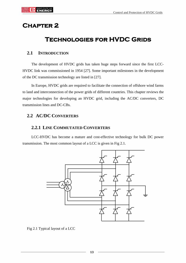
transmission. The most common layout of a LCC is given in Fig 2.1.
Fig 2.1 Typical layout of a LCC

Control and Protection of HVDC Grids
14
The thyristor valves are arranged in two Graetz bridges [28] for AC to DC conversion
in order to cancel the 6-pulse harmonics on both the AC and DC sides [29]. Only if there is a
positive voltage applied between the anode and the cathode of a thyristor, the thyristor can
conduct current from an AC system by having a firing pulse which is generated by
synchronising the AC system. This firing pulse can be delayed from an instant when voltage
starts to become positive. This is also known as the delay angle. The change of the delay
angle will generate different average DC voltages (i.e. an increase of delay angle leads to a
decrease of average DC voltage) in order to control the power flow through the converter.
The polarity of average DC voltage can be reversed (when delay angle > 90º) to change the
direction of power delivery while the current flow is unidirectional due to the physical limit
of a thyristor.
2.2.2 TWO-LEVEL VOLTAGE SOURCE CONVERTERS
VSC technology is been actively developed for HVDC. Early VSC-HVDC links (e.g.
Gotland HVDC Light [30]) were built based on Pulse Width Modulation (PWM) controlled
two-level VSCs (see Fig 2.2).
Fig 2.2 Architecture of a 2-level VSC
Each two-level VSC has six valves that contain fully controllable switching devices
(e.g. IGBTs in the most applications) connected in series to obtain a system-level DC voltage.
These switching devices depend on a gate signal for their switching (turn on or off) operation.
The gate signals can be generated using PWM technique (see Fig 2.3). Modulating the width
of pulse is based on the comparison between a carrier waveform and a reference waveform. A

Control and Protection of HVDC Grids
15
switching device turns on if the reference waveform ascends above a carrier waveform and
vice versa. This will create an output sinusoidal waveform with high frequency harmonics.
Therefore, phase reactors in combination with AC filters are needed for filtering the high
frequency harmonics. Increasing the frequency of carrier waveform (i.e. switching frequency)
will allow the use of filters with smaller sizes and thus bring down the cost of phase reactors
and AC filters. However, this will simultaneously increase the switching losses. A typical
switching frequency of 1 kHz to 2 kHz is used in most two-level VSC-HVDC practice [31] as
a trade-off of harmonics and switching losses.
t
+Udc/2
Carrier
-Udc/2
t
+Udc/2
-Udc/2Reference
Output
Fundamental
Fig 2.3 Sinusoidal Pulse Width Modulation
2.2.3 MULTI-LEVEL MODULAR CONVERTERS
The MMC was used as a utility STATCOM [32] and has soon become a viable solution
for VSC-HVDC network since 2010 when the first MMC based HVDC link (i.e. Trans Bay
Cable Project) was commissioned [33].
Within an MMC, each valve (see Fig 2.4 (a)) has hundreds of sub-modules (SMs) connected
as “chain links” where the switching of each SM is individually controlled to produce a
sinusoidal voltage (see Fig 2.4 (b)).
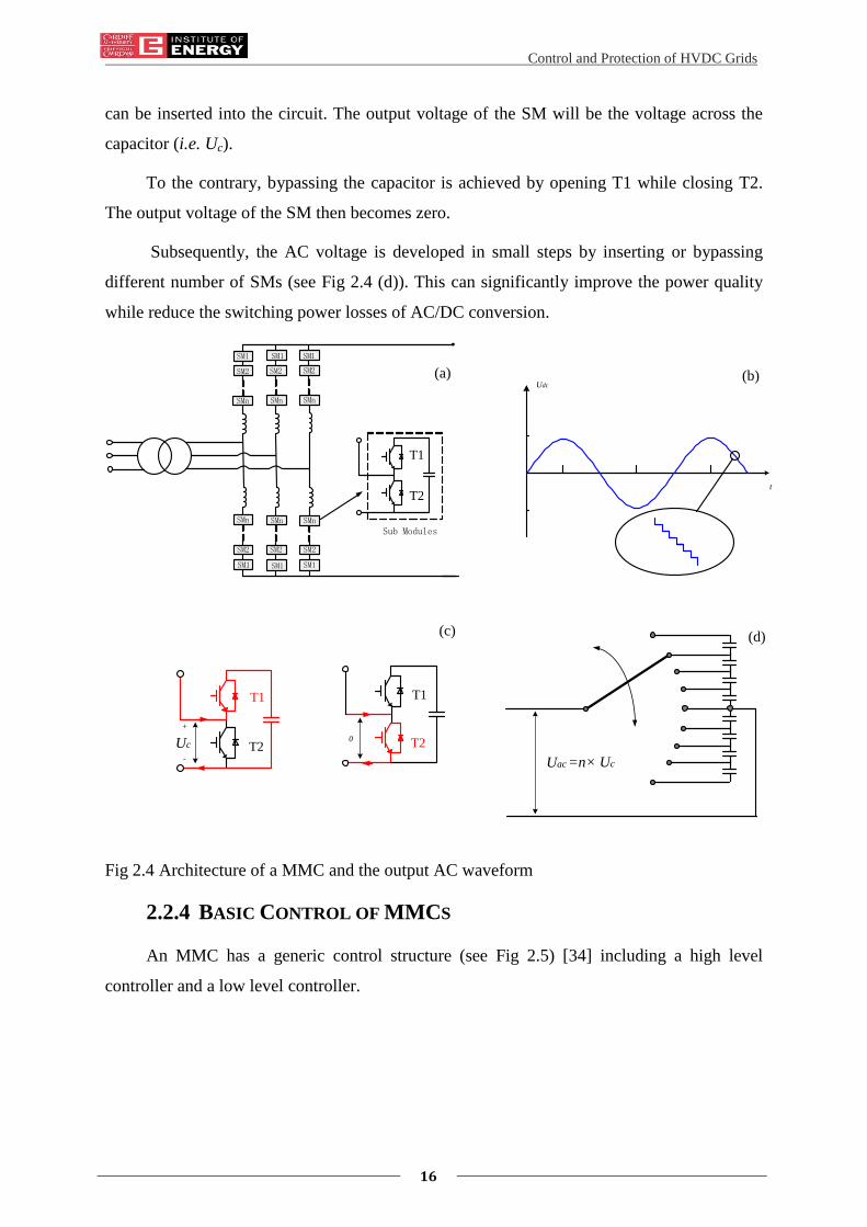
The Fig 2.4 (c) and Fig 2.4 (d) present the switching of IGBT and the establishment of
AC voltage. A SM is composed of one half bridge (with two IGBTs) and a capacitor (see Fig
2.4 (c)). By closing the upper IGBT (T1) and opening the lower IGBT (T2), the capacitor
Control and Protection of HVDC Grids
16
can be inserted into the circuit. The output voltage of the SM will be the voltage across the
capacitor (i.e. Uc).
To the contrary, bypassing the capacitor is achieved by opening T1 while closing T2.
The output voltage of the SM then becomes zero.
Subsequently, the AC voltage is developed in small steps by inserting or bypassing
different number of SMs (see Fig 2.4 (d)). This can significantly improve the power quality
while reduce the switching power losses of AC/DC conversion.
SM1
SM2
SMn
SM1
SM2
SMn
SM1
SM2
SMn
SM1
SM2
SMn
SM1
SM2
SMn
SM1
SM2
SMn
Sub Modules
t
Udc
T1
T2
Uac
T1
T2 T2
T1
Uc
+
-
0
(a) (b)
(c) (d)
=n× Uc
Fig 2.4 Architecture of a MMC and the output AC waveform
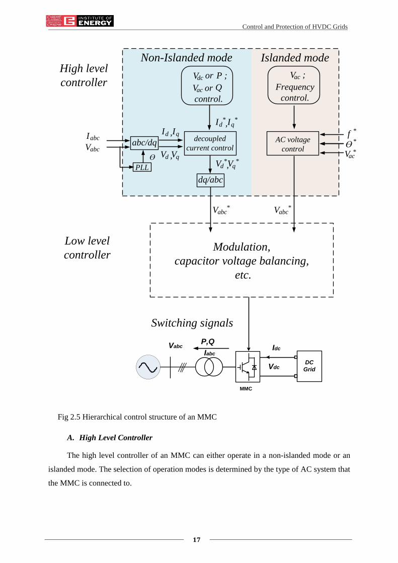
2.2.4 BASIC CONTROL OF MMCS
An MMC has a generic control structure (see Fig 2.5) [34] including a high level
controller and a low level controller.
Control and Protection of HVDC Grids
17
MMC
VdcDC
Grid
IdcVabc
Iabc
P,Q
acV
Frequency
control.
;P ;dcV
acV Q
or
or
control.
decoupled
current control
PLL
Ɵ
abcI
abcVabc/dq
dq/abc
AC voltage
control
f *
Ɵ *
acV *
abcV *abcV *
High level
controller
Low level
controllerModulation,
capacitor voltage balancing,
etc.
Switching signals
Islanded modeNon-Islanded mode
d I *qI *
,
d V *qV *
,
d I qI,
d V qV,
Fig 2.5 Hierarchical control structure of an MMC
A. High Level Controller
The high level controller of an MMC can either operate in a non-islanded mode or an
islanded mode. The selection of operation modes is determined by the type of AC system that
the MMC is connected to.

Control and Protection of HVDC Grids
18
The non-islanded mode is used when an MMC converter is connected to an AC
system with active synchronous generation (e.g. strong AC grid). The standard hierarchy of
the non-islanded mode is shown in Fig 2.6 and Fig 2.7.
Fig 2.6 shows the outer control loop of the non-islanded mode where two variables can
be regulated at a time. For example, it can control the active power (P) and reactive power (Q)
simultaneously. A simple approach is to use PI control units to regulate both variables
respective to the reference orders (P* and Q
*) given by a system operator. This will generate
two current references (i.e. Iq* and Id
*) which are further sent to the “decoupled current
control” block as shown in Fig 2.5.
PI
PI
P
P*
dcV *
dcV
PI dcI *
dcI
PI
PI
*
acV *
acV
Q
Q
Current Limiter
qI *
dI *
Outer control loop
within non-island
mode
dI ’
qI ’
Fig 2.6 Outer control loop for non-islanded control mode
The “decoupled current control” block is designed for regulating the direct and
quadrature components of the AC current (i.e. Id and Iq). The measurements of AC current are
transformed into direct-quadrature frame using the abc to dq transformation (i.e. park
transformation) as shown in Fig 2.5. A phase lock loop (PLL) is required for locking the
voltage at the AC grid and generating the reference angle (Ɵ) for abc to dq transformation.
Currents Id and Iq are then regulated regarding to the current reference given by the
outer control loop (see Fig 2.7). This will create the AC voltage references in d-q frame (i.e.
Vd* and Vq
*) which are then transferred back to abc frame.

Control and Protection of HVDC Grids
19
Id
Iq
PI
PI
ωL
ωL
Ɵ
Vd
dI *
qI *
dq/abc
abcV *dV *
qV *
Fig 2.7 Inner decoupled current control for non-islanded control mode
Alternatively, the islanded mode is used for converters connected to very weak AC
systems. Two typical weak AC systems are wind parks and islanded loads. For example, an
offshore wind parks consist of arrays of wind turbines connected to an AC grid with
practically no local load. For these schemes the HVDC grid constitutes the only way of
evacuating the generated power out of the system and as such the frequency of offshore AC
voltage must be maintained within an acceptable range to keep the offshore power balanced
(i.e. generated wind power matches the power flow through converter plus the power losses).
Similarly, in cases the HVDC grid connected to islanded loads, an AC voltage must be
established and the power in-feed into the islanded must match the load requirements to
maintain the frequency of AC voltage. Therefore, in either case an AC voltage should be
established with its frequency regulated at acceptable values. This is achieved by operating
the MMCs in the islanded mode.
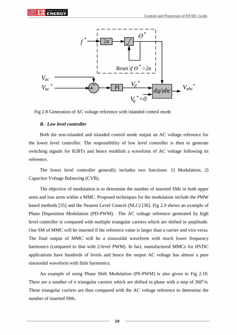
Fig 2.8 shows the control blocks with the islanded mode. Its inputs include an AC
voltage amplitude reference (Vac*), a measured AC voltage (Vac) and a frequency reference (f
*). The PI controller eliminates the steady state error between Vac
* and Vac and generates a d-
axis voltage reference (Vd*) while the q-axis voltage reference (Vq
*) can be set to zero directly
as no variable needs to be controlled via the q-axis in the islanded mode. The angle reference
for dq to abc transformation is created by an independent oscillator. This is essentially
different to that in the non-islanded mode where the angle reference is generated by a PLL
locking the voltage at an active AC source. The final output of the islanded mode is a voltage
reference in abc frame (Vabc).
Control and Protection of HVDC Grids
20
abcV *
*f 2π ∫
Ɵ *
Reset if Ɵ >2π *
dq/abcPI acV *
acV
dV *
qV =0*
Fig 2.8 Generation of AC voltage reference with islanded control mode
B. Low level controller
Both the non-islanded and islanded control mode output an AC voltage reference for
the lower level controller. The responsibility of low level controller is then to generate
switching signals for IGBTs and hence establish a waveform of AC voltage following its
reference.
The lower level controller generally includes two functions: 1) Modulation; 2)
Capacitor Voltage Balancing (CVB).
The objective of modulation is to determine the number of inserted SMs in both upper
arms and low arms within a MMC. Proposed techniques for the modulation include the PMW
based methods [35] and the Nearest Level Control (NLC) [36]. Fig 2.9 shows an example of
Phase Disposition Modulation (PD-PWM). The AC voltage reference generated by high
level controller is compared with multiple triangular carriers which are shifted in amplitude.
One SM of MMC will be inserted if the reference value is larger than a carrier and vice versa.
The final output of MMC will be a sinusoidal waveform with much lower frequency
harmonics (compared to that with 2-level PWM). In fact, manufactured MMCs for HVDC
applications have hundreds of levels and hence the output AC voltage has almost a pure
sinusoidal waveform with little harmonics.
An example of using Phase Shift Modulation (PS-PWM) is also given in Fig 2.10.
There are a number of n triangular carriers which are shifted in phase with a step of 360o/n.
These triangular carriers are then compared with the AC voltage reference to determine the
number of inserted SMs.

Control and Protection of HVDC Grids
21
Fundamental
Multiple Carriers
t
+Udc/2
-Udc/2
Reference
Output
t
+Udc/2
-Udc/2
Fig 2.9 Phase disposition modulation
t
Reference
n carrier waves 360° /
t
+Udc/2
-Udc/2
+Udc/2
-Udc/2
Output
Fig 2.10 Phase shift modulation
t
+Udc/2
-Udc/2
Reference
t
+Udc/2
-Udc/2
Discretisation
Usample
Round
Usample
NSM =USM
Fig 2.11 Nearest level control
Alternatively, the NLC can be used for the modulation (see Fig 2.11). With this
method, the AC voltage reference will firstly be discretised and output a reference Usample.
The number of inserted SMs (Na) is then estimated by dividing Usample with the average
capacitor voltage of SMs (USM). The calculated NSM is usually not an integer number and
hence rounding is needed to obtain an exact number for the inserted SMs.

Control and Protection of HVDC Grids
22
NSM
USM1
USM2
...USMn
Sorting
iarm
Generating switching
signals
If (iarm>0)&(insert SM)
Insert the SM with lowest voltage
If (iarm<0)&(insert SM)
If (iarm>0)&(bypass SM)
If (iarm<0)&(bypass SM)
Function when Nsm changes
Insert the SM with highest voltage
Bypass the SM with highest voltage
Bypass the SM with lowest voltage
iarm>0: charge
iarm<0: discharge
T1
T2 T2
T1
C Ciarm iarm
T1
T2 T2
T1
C Ciarm iarm+ + + +
1.Charge 2.Prevent charging 3.Discharge 4.Prevent discharging
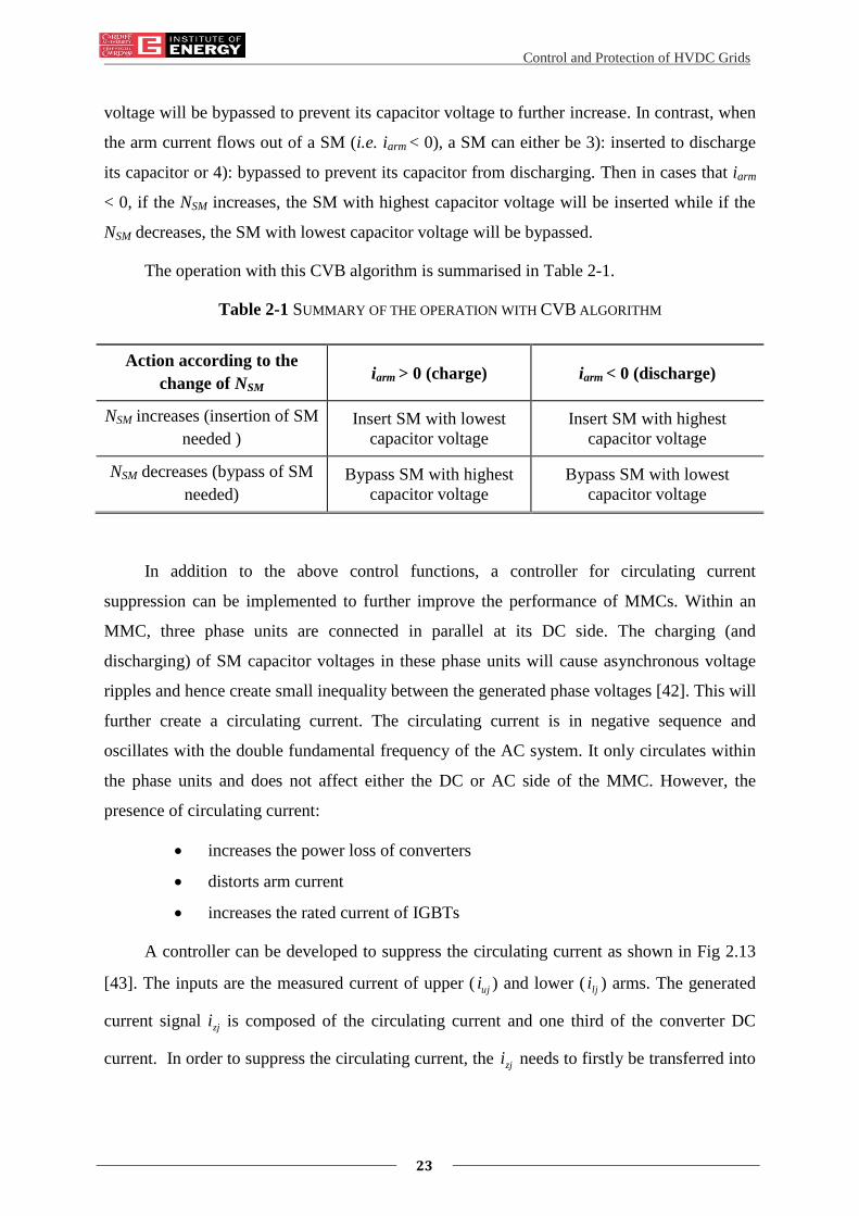
Fig 2.12 Control of CVB
The obtained number of inserted SMs will further be sent to another important block
for CVB. The control of CVB aims to stabilise the capacitor voltage of each SM around the
average value (USM) and hence prevent the capacitor voltage from diverging. Different
algorithms for CVB have been proposed in [37] to [41] while a conventional approach [41] is
shown in Fig 2.12.
The input into the control block including the requested number of inserted SM (NSM),
the direction of arm current (iarm) and the SM capacitor voltages which are sorted from the
highest value to the lowest one. The CVB only functions at the instants of NSM changing. For
example, when NSM increases by 1, the CVB decides which SM should be inserted and
conversely, when NSM decreases by 1, the CVB determines which SM should be bypassed.
The decision of which SM should be inserted or bypassed is made based on the four
operating states of SMs. When the arm current feeds into a SM (i.e. iarm > 0), a SM can either
be 1): inserted to charge its capacitor (C) or 2): bypassed to prevent its capacitor from
charging. In order to balance the capacitor voltage, the SM with the lowest capacitor voltage
will be inserted based on request and the capacitor voltage will be charged to higher values.
Similarly, if bypass operation is requested (when iarm > 0), the SM with the highest capacitor
Control and Protection of HVDC Grids
23
voltage will be bypassed to prevent its capacitor voltage to further increase. In contrast, when
the arm current flows out of a SM (i.e. iarm < 0), a SM can either be 3): inserted to discharge
its capacitor or 4): bypassed to prevent its capacitor from discharging. Then in cases that iarm
< 0, if the NSM increases, the SM with highest capacitor voltage will be inserted while if the
NSM decreases, the SM with lowest capacitor voltage will be bypassed.
The operation with this CVB algorithm is summarised in Table 2-1.
Table 2-1 SUMMARY OF THE OPERATION WITH CVB ALGORITHM
Action according to the
change of NSM iarm > 0 (charge) iarm < 0 (discharge)
NSM increases (insertion of SM
needed )
Insert SM with lowest
capacitor voltage
Insert SM with highest
capacitor voltage
NSM decreases (bypass of SM
needed)
Bypass SM with highest
capacitor voltage
Bypass SM with lowest
capacitor voltage
In addition to the above control functions, a controller for circulating current
suppression can be implemented to further improve the performance of MMCs. Within an
MMC, three phase units are connected in parallel at its DC side. The charging (and
discharging) of SM capacitor voltages in these phase units will cause asynchronous voltage
ripples and hence create small inequality between the generated phase voltages [42]. This will
further create a circulating current. The circulating current is in negative sequence and
oscillates with the double fundamental frequency of the AC system. It only circulates within
the phase units and does not affect either the DC or AC side of the MMC. However, the
presence of circulating current:
increases the power loss of converters
distorts arm current
increases the rated current of IGBTs
A controller can be developed to suppress the circulating current as shown in Fig 2.13
[43]. The inputs are the measured current of upper ( uji ) and lower ( lji ) arms. The generated
current signal zji is composed of the circulating current and one third of the converter DC
current. In order to suppress the circulating current, the zji needs to firstly be transferred into

Control and Protection of HVDC Grids
24
the d-q frame (to generate the direct fdi2 and quadrature components fqi2 ) with an angle
reference of the double fundamental frequency (2𝜔t) as the main frequency of circulating
current is the second harmonic of the AC system. Then by setting the references (i.e. reffdi _2
and reffqi _2 ) of fdi2 and fqi2 to zero while using PI controllers to eliminate the errors between
the references and measured currents, the circulating current can be suppressed. The final
output is the demanded voltage reference Vdiff_jref
which can be added to the AC voltage
reference Vabc* before modulation.
PI
PI
2ωL
2ωL
Vd
dq/abcdiff_ jV
refdV *
qV *
uji
lji
abc/dq
2ωt
= 02fd_ref I
= 02fq_ref I
2fd I
2fq I
2ωt
Fig 2.13 Circulating current suppression control
2.3 HVDC TRANSMISSION LINES
HVDC transmission can make use of OHLs and cables.
A. Overhead line
OHLs are the most economical means for bulk power over long distance due to its low
installation cost. The transmission capacity of an OHL is limited by the thermal rating of sag
and the annealing temperature of the conductor. The conducting material of OHLs can be
either copper or aluminium. The density and hence the weight of aluminium is lower than
those of copper. Moreover, aluminium has lower cost per kilogram. These make the
aluminium the preferred choice [44].
To date, the use of OHLs in HVDC projects has reached a voltage and power rating
reach at 1100 kV and 10 GW respectively [45]. The applications of OHLs in HVDC practice
are similar to those in AC systems. There is also no significant difference in the design of
towers for OHLs in HVDC and AC systems. However, HVDC OHLs have higher

Control and Protection of HVDC Grids
25
transmission capacity. It is studied that three-phase double circuit AC OHLs can have 40% to
80% more transmission capacity when they are converted and used as HVDC OHLs [44].
B. HVDC cable
HVDC cables can be used in submarine and underground applications. For example,
they can be used for connecting offshore wind farms to inland load centre and also power
transmission over long distance in the sea where the use of OHLs is no longer feasible.
Moreover, small right-of-way of HVDC cables makes them ideal for being used in land
power transmission including city areas.
HVDC cables consist of a conductor core, semiconductor screen, main insulation,
sheath, armouring, and related accessories. The different characteristics of dielectric materials
lead to different electrical, mechanical and thermal performance. HVDC cables are
categorised into five types according to the dielectrics [46][47] as oil-filled DC cable, mass-
impregnated cable (MI), extruded DC cable, gas insulated cable and superconducting cable.
With the practical HVDC projects, the MI cables (see Fig 2.14) and extruded cables (see Fig
2.15) have been mainly used.
MI cables are acknowledged as “solid” insulation system since there is no free oil
contained in the cable. The insulation of MI cables is made of mass-impregnated and non-
draining paper. High-density papers (≈1000 kg/cm3) can provide higher dielectric properties.
The cable length in principle is unlimited due to no external pressure and oil feeding request.
As a proven reliable cable technology, MI cables have been used in HVDC applications
for over 60 years. Recently, new insulation utilises laminated polymeric film and paper which
increases the maximum conductor temperature of MI cables from 55 °C to 85 °C. The MI
cable can hence be sized at higher rating. Such kind of MI cables has already been applied in
practice like the Westernlink project where the MI cables are rated at 600 kV and 2200 MW
[46].

Control and Protection of HVDC Grids
26
Fig 2.14 Mass-impregnated cables [47]
Fig 2.15 Extruded cables
Extruded cables are relatively new developments. Its major insulation material is cross-
linked polyethylene (XLPE). In 2002, the first extruded cables were developed in a
laboratory in Japan. To date, this cable technology has been applied in practical projects with
DC voltage rated up to 320 kV and active power rated up to 1000 MW. Moreover, ABB has
claimed that the first 525 kV, 2600 MW extruded cable system has been developed [26].
The extruded cables have advantages over MI cables as listed below [49]:
Have higher maximum conductor temperature, giving a more compact cable
for the same power rating;
Lighter moisture barriers can be used which makes the cable lighter;

Control and Protection of HVDC Grids
27
Joining of extruded cables is much simpler and requires less skill.
However, the extruded cables are vulnerable to voltage polarity reversal which will
enhance the electric field and cause permanent failure in the insulation of extruded cables.
Therefore, the extruded cables are used in VSC based HVDC networks which operations
without the requirement of voltage polarity reversal. LCC-HVDC links still utilise MI cables
since the change of power flow direction requires the voltage polarity reversal.
2.4 DC CIRCUIT BREAKERS FOR HVDC GRID PROTECTION
2.4.1 HVDC NETWORK PROTECTION
The protection of HVDC networks remains a main challenge for developing HVDC
grids. A DC network has in general low inductance. Under the presence of a DC fault, a DC
network will exhibit a higher fault current rise time and a faster fault propagation time when
compared to an AC fault occurring in an AC network where the propagation of fault current
is limited by the relatively large system inductance. Moreover, the DC fault current does not
have a natural zero-crossing. These could bring difficulties in HVDC network protection,
particularly HVDC grids.
To date, the protection of P2P VSC-HVDC links has become relatively mature while
new protection components, such as DC-CBs, will be needed for protecting HVDC grids.
This is descripted in detail as below.
A. Point to point HVDC links
Fig 2.16 shows a typical protection circuit for a P2P HVDC link using VSCs, AC-CBs
and DC disconnectors.
AC
breaker 1DC link
AC
breaker 2VSC1 VSC2
Disconnectors Disconnectors
Fig 2.16 Protection of a P2P HVDC link
Following a DC fault, DC voltage will rapidly decrease, resulting in a fast increase of
DC current. Current (and voltage) sensors located at each VSC station are employed to detect
the first wave-front of fault current (and voltage). An overcurrent and undervoltage criterion
is used to block the IGBTs within the VSCs. As a result the fault current will flow from the
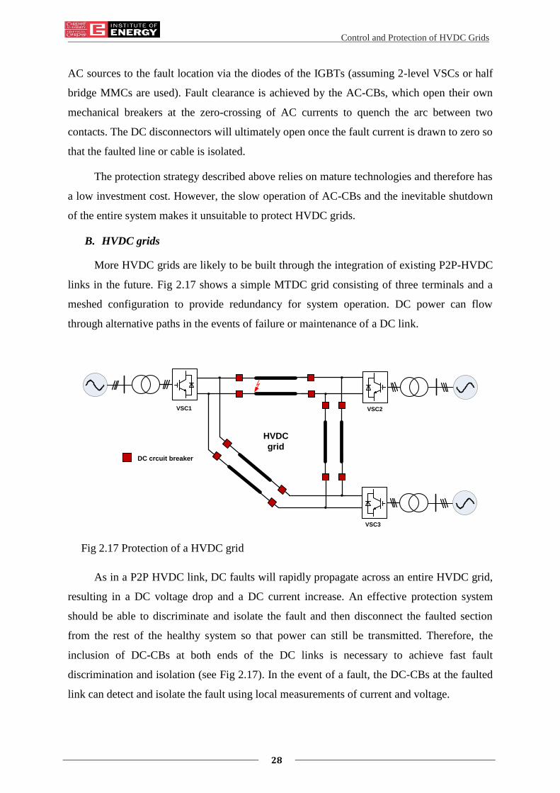
Control and Protection of HVDC Grids
28
AC sources to the fault location via the diodes of the IGBTs (assuming 2-level VSCs or half
bridge MMCs are used). Fault clearance is achieved by the AC-CBs, which open their own
mechanical breakers at the zero-crossing of AC currents to quench the arc between two
contacts. The DC disconnectors will ultimately open once the fault current is drawn to zero so
that the faulted line or cable is isolated.
The protection strategy described above relies on mature technologies and therefore has
a low investment cost. However, the slow operation of AC-CBs and the inevitable shutdown
of the entire system makes it unsuitable to protect HVDC grids.
B. HVDC grids
More HVDC grids are likely to be built through the integration of existing P2P-HVDC
links in the future. Fig 2.17 shows a simple MTDC grid consisting of three terminals and a
meshed configuration to provide redundancy for system operation. DC power can flow
through alternative paths in the events of failure or maintenance of a DC link.
HVDC
grid
VSC1 VSC2
VSC3
DC crcuit breaker
Fig 2.17 Protection of a HVDC grid
As in a P2P HVDC link, DC faults will rapidly propagate across an entire HVDC grid,
resulting in a DC voltage drop and a DC current increase. An effective protection system
should be able to discriminate and isolate the fault and then disconnect the faulted section
from the rest of the healthy system so that power can still be transmitted. Therefore, the
inclusion of DC-CBs at both ends of the DC links is necessary to achieve fast fault
discrimination and isolation (see Fig 2.17). In the event of a fault, the DC-CBs at the faulted
link can detect and isolate the fault using local measurements of current and voltage.

Control and Protection of HVDC Grids
29
Notice that the main protection system of an HVDC grid should avoid the use of
communication as this may cause large time delays and would require an adequate
synchronisation of DC-CBs. Moreover, a fault will not only affect a specific DC line but also
other sections of the network. Therefore, the protection system must be designed to
discriminate the healthy circuits from the faulted section. This can be done by comparing the
currents and voltages measured at the faulted lines with those of the healthy circuits. The DC-
CBs located at non-faulted lines should be kept closed throughout the fault.
2.4.2 PROPOSED DC-CBS
The demand of HVDC grid protection becomes a key driver of developing DC-CBs. A
desirable DC-CB should be able to clear a DC fault within milliseconds and hence prevent
the fault from affecting the healthy circuits significantly. Furthermore, it should be reliable
and not affect the normal operation of a HVDC grid (e.g. cause large power loss). There is no
high voltage DC-CBs commercially available at present. However, several potential solutions
are provided as: the mechanical resonant breakers, the full solid-state breakers and the hybrid
HVDC breakers.
A. Mechanical resonant breakers
There are passive mechanical resonance breakers and active mechanical resonance
breakers.
The passive mechanical resonance breakers are proposed in [50] and [51]. Fig 2.18
shows an example of a passive mechanical resonance breaker. It operates to create a current
zero-crossing and hence interrupt the DC fault current using mechanical switches.
The resonance branch consists of an L-C commutation circuit which is in parallel with
the low-loss mechanical breaker in primary branch. Current flows through the primary branch
during the normal operation of a HVDC system. Once a DC fault occurs, a resonance current
will be excited passively by the arc of fault. This will further cause current oscillation in the
primary branch and hence create a zero-crossing after one or a few cycles. The mechanical
switch can then interrupt the arc at the first zero-crossing and the fault energy will be absorbed
by the surge arresters.
The passive mechanical resonant breakers have no semiconductor switches and hence
have low costs. The power losses caused by this type of breakers are also low as the primary
branch conducting current during system normal operation. However, the long interruption
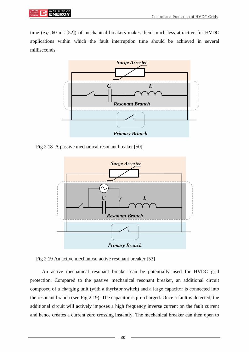
Control and Protection of HVDC Grids
30
time (e.g. 60 ms [52]) of mechanical breakers makes them much less attractive for HVDC
applications within which the fault interruption time should be achieved in several
milliseconds.
Surge Arrester
Resonant Branch
Primary Branch
C L
Fig 2.18 A passive mechanical resonant breaker [50]
Fig 2.19 An active mechanical active resonant breaker [53]
An active mechanical resonant breaker can be potentially used for HVDC grid
protection. Compared to the passive mechanical resonant breaker, an additional circuit
composed of a charging unit (with a thyristor switch) and a large capacitor is connected into
the resonant branch (see Fig 2.19). The capacitor is pre-charged. Once a fault is detected, the
additional circuit will actively imposes a high frequency inverse current on the fault current
and hence creates a current zero crossing instantly. The mechanical breaker can then open to
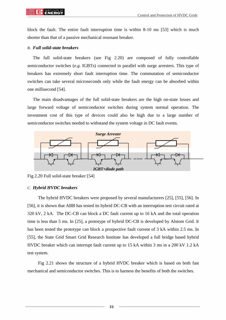
Control and Protection of HVDC Grids
31
block the fault. The entire fault interruption time is within 8-10 ms [53] which is much
shorter than that of a passive mechanical resonant breaker.
B. Full solid-state breakers
The full solid-state breakers (see Fig 2.20) are composed of fully controllable
semiconductor switches (e.g. IGBTs) connected in parallel with surge arresters. This type of
breakers has extremely short fault interruption time. The commutation of semiconductor
switches can take several microseconds only while the fault energy can be absorbed within
one millisecond [54].
The main disadvantages of the full solid-state breakers are the high on-state losses and
large forward voltage of semiconductor switches during system normal operation. The
investment cost of this type of devices could also be high due to a large number of
semiconductor switches needed to withstand the system voltage in DC fault events.
Surge Arrester
IGBT+diode path
Fig 2.20 Full solid-state breaker [54]
C. Hybrid HVDC breakers
The hybrid HVDC breakers were proposed by several manufacturers [25], [55], [56]. In
[56], it is shown that ABB has tested its hybrid DC-CB with an interruption test circuit rated at
320 kV, 2 kA. The DC-CB can block a DC fault current up to 16 kA and the total operation
time is less than 5 ms. In [25], a prototype of hybrid DC-CB is developed by Alstom Grid. It
has been tested the prototype can block a prospective fault current of 3 kA within 2.5 ms. In
[55], the State Grid Smart Grid Research Institute has developed a full bridge based hybrid
HVDC breaker which can interrupt fault current up to 15 kA within 3 ms in a 200 kV 1.2 kA
test system.
Fig 2.21 shows the structure of a hybrid HVDC breaker which is based on both fast
mechanical and semiconductor switches. This is to harness the benefits of both the switches.

Control and Protection of HVDC Grids
32
Residual Current
Breaker
(RCB)
Ultrafast Disconnector
(UFD)
Load Commutation Switch
(LCS)
Main Breaker
Surge Arrester(MOV)
Fig 2.21 Hybrid HVDC circuit breaker [56]
The low-loss branch of the breaker includes an ultrafast disconnector (UFD) and a load
commutation switch (LCS). The main breaker is packed with series-connected IGBTs for fault
interruption. The surge arresters (MOV) are for fault energy absorption.
During normal operation, current flows through the low-loss branch only as shown in
Fig 2.22 (a). Since the low-loss branch has only a few semiconductor switches, the on-state
losses are much lower compared to the full solid-state breakers.
If a DC fault happens at t1, the fault current flowing through the low-loss branch will rise
rapidly as shown in Fig 2.23. The relay of the DC-CB will take some delay to detect the fault
and the load commutation switch will block immediate at t2 and hence commutate the current
to flow through the main breaker branch (see Fig 2.23).
The ultrafast disconnector (UFD) will then start to open as the current at this branch
reaches zero. This action causes delays in the order of milliseconds. The main breaker will
have to keep closed until the UFD blocked. Therefore, the fault current flowing through the
main breaker branch will keep rising from Itrip to Ipeak.
Once the UFD is blocked, the main breaker which is based on semiconductor switches
can then trip to isolate the fault within microseconds. The fault current will thus flow through
the surge arrester (MOV) (see Fig 2.22 (c)) and the fault energy is absorbed by the surge
arresters, taking a time from t3 to t4 (within several hundred microseconds) (see Fig 2.23).
Once the fault current is cleared, the residual current breaker (RCB) will ultimately open
to prevent the surge arrester from thermal overloaded (see Fig 2.22 (d)).

Control and Protection of HVDC Grids
33
The entire interruption time of a hybrid HVDC circuit breaker is in milliseconds. It also
has low on-state losses during system normal operation. These features make hybrid HVDC
circuit breakers ideal for HVDC grid protection.
Fig 2.22 Working principle of a hybrid HVDC breaker
Fig 2.23 Process of fault current interruption

Control and Protection of HVDC Grids
34
2.5 SUMMARY
This chapter introduced the main HVDC technologies including: AC/DC converters,
DC transmission lines and DC-CBs. The topologies and operation principles of LCCs and
VSC are described. The review highlights on one particular type of the VSCs – the modular
multi-level converters (MMCs).
The basic control of an MMC has been discussed in details. It has a hierarchical control
structure with both a high level and a low level controller. With the high level controller, an
MMC can either operate in non-islanded mode or islanded mode. Both modes allow the
MMC to control certain items (e.g. active/reactive power, voltage and frequency) and
generate AC voltage references for the low level controller. The low level controller has two
essential functions – modulation and CVB. The modulation determines number of inserted
SM within the MMC according to the AC voltage references given by the high level
controller. The CVB acts to keep the voltage of SM capacitors balanced. The low level
controller will then output the switch signals for each IGBT.
The DC transmission lines including OHLs and cables have been described. The
application of OHLs in HVDC systems is similar to that in AC systems while the
transmission capacity is much higher comparing the DC to the AC. DC cables can be used in
offshore and city areas. Different types of DC cables are also introduced, focusing on the
impregnated cables and the extruded cables.
The basic protection of a HVDC network has been described. The protection for P2P
HVDC link can be based on AC circuit breakers while the protection for HVDC grids will
reply on DC-CBs. Different types of proposed DC-CBs including full the mechanical
resonant breakers, the full solid-state breakers and the hybrid DC-CBs are then presented.
The mechanical resonant breakers have long fault interruption time while the full solid-state
breakers have high on-state losses. The hybrid DC-CBs consist of both mechanical and
semiconductor switches and hence have the advantages of low on-state losses and also short
fault interruption time. Therefore, the hybrid DC-CBs appear to be a preferable option for
HVDC grid protection in the future.

Control and Protection of HVDC Grids
35
Chapter 3
3. Control of an HVDC Grid
3.1 INTRODUCTION
Much research has been done regarding the control and coordination of VSC converters
in an MTDC or HVDC grid. Amongst those, one underlying concept is the DC voltage droop
control.
In this chapter, the control concept has been further developed to use alternative droop
characteristics on each converter. This approach allows precise converter current regulation
during normal operation and stabilises DC voltage during power disturbance. Control
algorithms of alterative droop characteristics are provided and interactions of different
control characteristics are analysed. Guidelines of choosing droop characteristics are
provided by comparing their current control performance. Moreover, potential risk of having
multiple cross-over in control characteristics is uncovered. The design of values of droop
characteristics is then also discussed to avoid the multiple cross-over.
3.2 HVDC GRID CONTROL REVIEW
The control of a HVDC grid has an important objective: balancing the power import
and export (plus power loss) within a HVDC grid. Any power unbalance will lead to a
variation of DC voltage. Therefore, it is important to maintain the DC voltage within a
defined band in a HVDC grid. The regulation of DC voltage is achieved via the control for
AC/DC converter stations. At least one converter controls the DC voltage while other
converters can either regulate their own converter power or share the responsibility of voltage
control. Moreover, at the AC side, converters are expected to establish AC voltages for weak
AC systems and to exchange reactive power with strong AC systems.
3.2.1 REQUIREMENT FOR CONTROLLING AN HVDC GRID
There are some analogies between AC and DC systems (See Table 3-1) which can be
considered in the control design for a HVDC grid. The DC voltage is the indication of power
balance in a DC system. Power surplus in a HVDC network will lead to DC voltage increase
and power deficit will cause DC voltage decrease. However, the DC voltage is not uniform

Control and Protection of HVDC Grids
36
across the network; this requires consideration of the DC voltage drops along the circuits for
active power balancing control. Moreover, the DC power flow through DC branches is
related to the voltage difference between DC nodes. The control of power flow through lines
thus requires consideration of DC voltage difference.
There are no directly connected generators or motors in the DC system which can
provide large inertia in a power grid. This implies that the control of power balance should
be more stringent and faster than in AC systems to avoid system overvoltage during events
such as power imbalance. Communication should be minimised to reduce undesirable time
delays. Other control requirements include [13] [57]:
High reliability: the control of a HVDC grid must be robust to system disturbances
and ensure fault ride-through.
Back-up systems: the DC voltage control is recommended to be duplicated as
redundancy to avoid collapse of the entire system during an outage of one DC voltage
control converter.
Precise power/current control: the control design should allow the converter power or
current to be regulated at desired values. The Power/current flow through DC
branches cannot be fully controlled by VSCs. Overloading of DC branches should be
avoided by using additional control devices (e.g. DC-PFCs).
Optimised operation: the use of converter capacity should be optimised. Maximum
steady-state voltage should be maintained to minimise system losses.
Flexible plug and play: more converters should be able to be connected without
changing the control of the existing system.
Table 3-1 COMPARISON OF AN AC GRID AND A DC GRID [57]
Droop Type AC GRID DC GRID
Indication of power balance Frequency (global) DC voltage (local)
Predominant impedance Inductance (X) Resistance (R)
Energy storage AC mechanical system DC capacitor
Active power flow Phase difference DC voltage difference
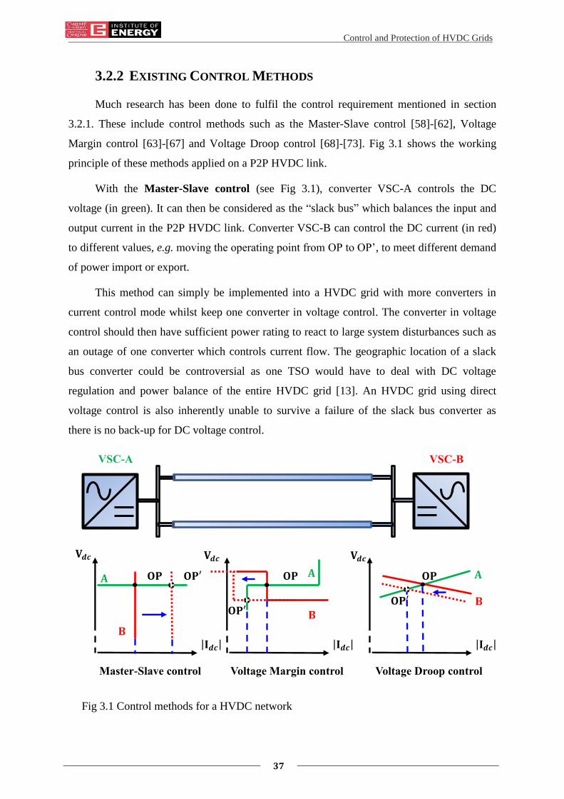
Control and Protection of HVDC Grids
37
3.2.2 EXISTING CONTROL METHODS
Much research has been done to fulfil the control requirement mentioned in section
3.2.1. These include control methods such as the Master-Slave control [58]-[62], Voltage
Margin control [63]-[67] and Voltage Droop control [68]-[73]. Fig 3.1 shows the working
principle of these methods applied on a P2P HVDC link.
With the Master-Slave control (see Fig 3.1), converter VSC-A controls the DC
voltage (in green). It can then be considered as the “slack bus” which balances the input and
output current in the P2P HVDC link. Converter VSC-B can control the DC current (in red)
to different values, e.g. moving the operating point from OP to OP’, to meet different demand
of power import or export.
This method can simply be implemented into a HVDC grid with more converters in
current control mode whilst keep one converter in voltage control. The converter in voltage
control should then have sufficient power rating to react to large system disturbances such as
an outage of one converter which controls current flow. The geographic location of a slack
bus converter could be controversial as one TSO would have to deal with DC voltage
regulation and power balance of the entire HVDC grid [13]. An HVDC grid using direct
voltage control is also inherently unable to survive a failure of the slack bus converter as
there is no back-up for DC voltage control.
Fig 3.1 Control methods for a HVDC network
VSC-A VSC-B
𝐕𝒅𝒄
𝐈𝒅𝒄
𝐎𝐏
𝐕𝒅𝒄
𝐈𝒅𝒄
𝐎𝐏 𝐎𝐏′
𝐎𝐏′
Master-Slave control Voltage Margin control
𝐕𝒅𝒄
𝐈𝒅𝒄
𝐎𝐏
Voltage Droop control
𝐎𝐏′
𝐀
𝐁
𝐁
𝐁
𝐀 𝐀

Control and Protection of HVDC Grids
38
An alternative for the control of an HVDC network is the Voltage Margin control.
With Voltage Margin control, each converter is equipped with both current control and
voltage control modes; however it operates under one mode at a time. Control modes switch
automatically whenever the operation point of any converter hits its current limit. The
example in Fig 3.1 shows that converter VSC-A switches from voltage to current control
when the current is reduced to a certain value (i.e. the operating point moves from OP to OP’).
The converter VSC-B then takes over the responsibility of DC voltage control. The advantage
of using this method is that an HVDC network can continue operating during a failure of a
converter in voltage control since the DC voltage control is replicated in multiple converters.
However, disadvantages of a centralised slack bus still remain; that is, converters may need a
larger power rating to be able to withstand large disturbances. Moreover, the selection of
current limits and voltage references should avoid multiple converters controlling DC voltage
simultaneously.
Another underlying concept for controlling an HVDC network is the Voltage Droop
control as shown in Fig 3.1. With this method, converters can regulate DC voltage by
adjusting the local converter DC currents, according to pre-defined DC voltage/DC current
characteristics. For example, in Fig 3.1 both converters VSC-A and VSC-B control the DC
voltage in different load conditions (i.e. moving operation point from OP to OP’). Therefore,
this method has the merit of distributed DC voltage control while minimising the reliance on
a communication system. The responsibility of regulating DC voltage is shared by multiple
converters and this makes the voltage droop control the most common concept for controlling
HVDC grids.
However, this method has the disadvantage of imprecise current control. A small
change in converter DC voltage could lead to a large variation in converter DC current due to
the flat droop.
Therefore, in this chapter, the Autonomous Converter Control (ACC) has been
developed to use alternative droops in order to improve the current control performance while
having distributed DC voltage control. This idea was initially proposed by Alstom Grid (now
GE Grid Solutions) in [57]. In 2013 and 2014, Alstom Grid worked with Cardiff University
on further developing this method. The main outcomes are given in the section 3.3 to section
3.6.

Control and Protection of HVDC Grids
39
3.3 AUTONOMOUS CONVERTER CONTROL (ACC)
The entire control structure of ACC includes one Grid Dispatch Centre (GDC) and all
local converter controllers (See Fig 3.2). The GDC has the overall responsibility for
determining the economic operation of the DC grid with changing generation and load
conditions. It acts by sending different control orders to the local converter controllers to
achieve a certain distribution of power flow. The dispatched control orders include:
A Load Reference Set Point (LRSP) which determines the DC voltage when a
converter operates at the ordered power.
A DC voltage/DC current characteristic which essentially defines the sensitivity
of DC voltage derivation to DC current change.
A Power Order that represents the desired converter power.
Fig 3.2 Control structure of the Autonomous Converter Control
DC
Lin
e S
yste
m
Communication
Grid
Dispatch Centre
Converter
Controller
Converter
Controller
Converter
Controller
Autonomous Converter
Converter
Control orders
Coordination
Control

Control and Protection of HVDC Grids
40
+Idc-Idc
Iord
LRSP
Vdc
Pord
=___LRSP
a
b
OP
Fig 3.3 DC converter droop characteristics
These control orders determine the control behaviours of each converter as shown in
Fig 3.3. In steady-state, the operating point (OP) of a converter should locate on the droop
line ab. Well dispatched control orders would locate the actual operating point very close to
the desired operating point, where the converter DC voltage is equal to the LRSP and
converter current is equal to the current demand. However, the control accuracy of current
and voltage is influenced in practice by the following items:
Measurement errors of DC voltage/DC current transducers;
Wrong computation of DC network resistance of GDC;
Telecommunication loss of GDC and local converters during change of
load/generation conditions;
Instantaneous power disturbance within a DC grid.
These items will cause the actual operating point to drift along the droop line away
from the desired operating point.
The slope of droop line is usually allocated a small value (say 3%-5%). This implies
that the converter DC current is very sensitive to the DC voltage. Small deviation of DC
voltage (∆𝑉𝑑𝑐) will lead to a large current error (∆𝐼𝑑𝑐) (see Fig 3.4). This will further cause
unwanted change of the power flow within a DC grid.
Therefore, in order to reduce the current error, a “current error function” has been
proposed as shown in Fig 3.5 (solid line). The current error function is a very high droop
(typically set to 200% [74]) inserted into the conventional droop characteristics. It aims to
reduce the current error at a converter for a small change in DC voltage level. The example
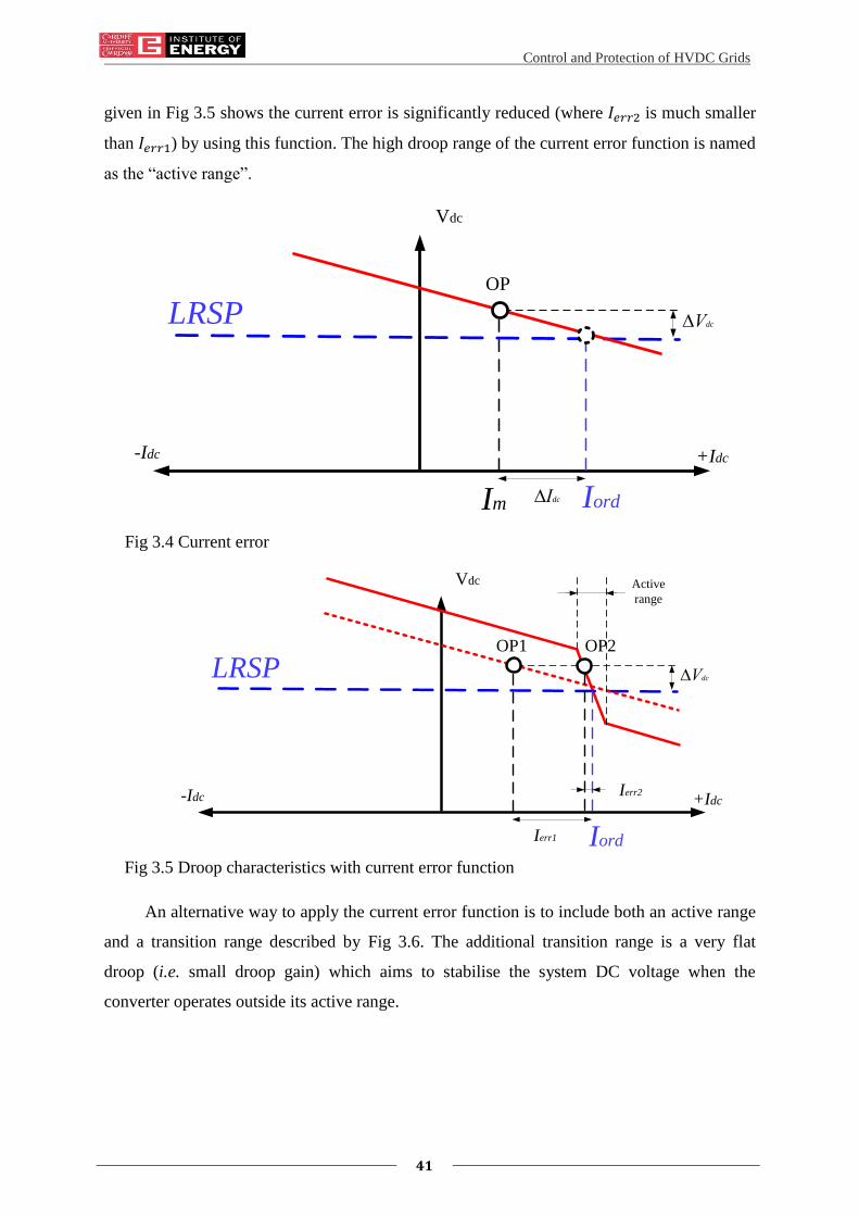
Control and Protection of HVDC Grids
41
given in Fig 3.5 shows the current error is significantly reduced (where 𝐼𝑒𝑟𝑟2 is much smaller
than 𝐼𝑒𝑟𝑟1) by using this function. The high droop range of the current error function is named
as the “active range”.
+Idc-Idc
Im
LRSP
Vdc
OP
Iord
∆Vdc
∆Idc
Fig 3.4 Current error
+Idc-Idc
LRSP
Vdc
OP1
Iord
∆Vdc
Ierr1
OP2
Active
range
Ierr2
Fig 3.5 Droop characteristics with current error function
An alternative way to apply the current error function is to include both an active range
and a transition range described by Fig 3.6. The additional transition range is a very flat
droop (i.e. small droop gain) which aims to stabilise the system DC voltage when the
converter operates outside its active range.

Control and Protection of HVDC Grids
42
c
+Idc-Idc
Iord
LRSP
Vdc
Active range
Transition range
Fig 3.6 Further modification on current error function
During normal system operation, one important criterion in evaluating HVDC grid
control is the DC current and voltage deviation from the original dispatched orders.
Assuming the control orders are well dispatched, the converters should operate inside the
active range of current error function, which leads to more precise current flow control.
In case of a telecommunications failure or large power disturbance, for safety
consideration, the transition range can provide a considerable amount of balancing current
due to its flat droop characteristics.
Terminologies are given for these droop characteristics as tabulated in Table 3-2. This
is arranged in an order that type 2 control will have the highest value of droop in all range
while type 0 control will have the smallest value of droop. Type 1 control is a trade-off
between type 0 and type 2 control. These terminologies are used within the remaining
contents in this thesis.
Table 3-2 TERMINOLOGIES FOR DIFFERENT DROOP TYPES
Droop Type Terminology
Conventional droop characteristics
(Fig 3.3) Type 0 control
Droop characteristics with modified
current error function (Fig 3.6) Type 1 control
Droop characteristics with current
error function (Fig 3.5) Type 2 control

Control and Protection of HVDC Grids
43
3.4 CONTROL ALGORITHM
All three droop types can be generated using the converter controller given in Fig 3.7.
Primary inputs sent from a Grid Dispatch Centre to the control system include a power order
(Pord), a LRSP, a DC Voltage/DC current slope (Droop) and a Droop type order (drp_typ).
Meanwhile, current-limit setting of active range (Ir1), transition range (Ir2) and a slope of
current error function (DroopH) needed to be defined.
LRSP
Pord ÷Iord
Droop
Idc
(Droop-DroopH)*IerrIerr
Ir2-|Ierr|
Ir2-Ir1
Vord
VSC
Idc
Vdc DC Grid
(Iord× Droop+LRSP)
(Idc× Droop)
Max
Min1
0
a
drp_type
0.5
Comparator1
Comparator2
1.5MAX
drp_type=0;Type 0 selected
drp_type=1;Type 1 selected
drp_type=2;Type 2 selected
Selection Block of Control Type
Comparator1: if drp_type>1.5, output 1; if drp_type≤ 1.5, output 0
Comparator2: if drp_type>0.5, output 1; if drp_type≤ 0.5, output 0
bc
Fig 3.7 Alternative droop control system
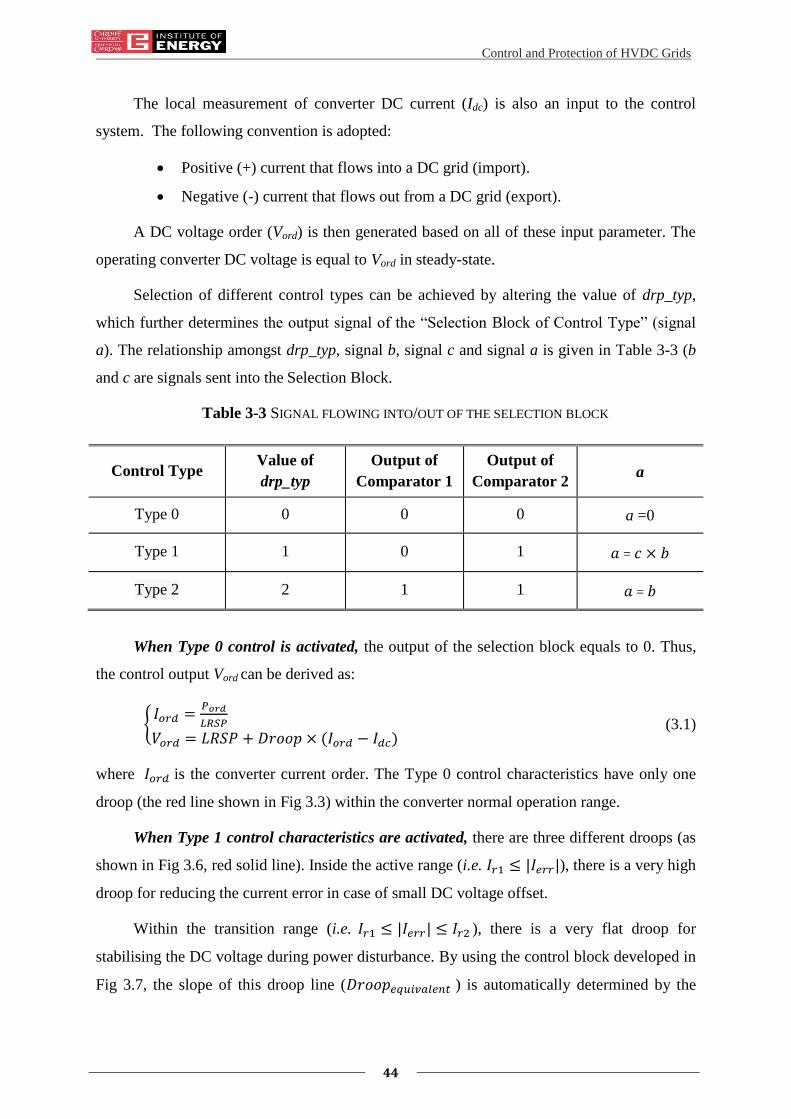
Control and Protection of HVDC Grids
44
The local measurement of converter DC current (Idc) is also an input to the control
system. The following convention is adopted:
Positive (+) current that flows into a DC grid (import).
Negative (-) current that flows out from a DC grid (export).
A DC voltage order (Vord) is then generated based on all of these input parameter. The
operating converter DC voltage is equal to Vord in steady-state.
Selection of different control types can be achieved by altering the value of drp_typ,
which further determines the output signal of the “Selection Block of Control Type” (signal
a). The relationship amongst drp_typ, signal b, signal c and signal a is given in Table 3-3 (b
and c are signals sent into the Selection Block.
Table 3-3 SIGNAL FLOWING INTO/OUT OF THE SELECTION BLOCK
Control Type Value of
drp_typ
Output of
Comparator 1
Output of
Comparator 2 a
Type 0 0 0 0 a =0
Type 1 1 0 1 𝑎 = 𝑐 × 𝑏
Type 2 2 1 1 𝑎 = 𝑏
When Type 0 control is activated, the output of the selection block equals to 0. Thus,
the control output Vord can be derived as:
𝐼𝑜𝑟𝑑 =
𝑃𝑜𝑟𝑑
𝐿𝑅𝑆𝑃
𝑉𝑜𝑟𝑑 = 𝐿𝑅𝑆𝑃 + 𝐷𝑟𝑜𝑜𝑝 × (𝐼𝑜𝑟𝑑 − 𝐼𝑑𝑐) (3.1)
where 𝐼𝑜𝑟𝑑 is the converter current order. The Type 0 control characteristics have only one
droop (the red line shown in Fig 3.3) within the converter normal operation range.
When Type 1 control characteristics are activated, there are three different droops (as
shown in Fig 3.6, red solid line). Inside the active range (i.e. 𝐼𝑟1 ≤ 𝐼𝑒𝑟𝑟 ), there is a very high
droop for reducing the current error in case of small DC voltage offset.
Within the transition range (i.e. 𝐼𝑟1 ≤ 𝐼𝑒𝑟𝑟 ≤ 𝐼𝑟2 ), there is a very flat droop for
stabilising the DC voltage during power disturbance. By using the control block developed in
Fig 3.7, the slope of this droop line (𝐷𝑟𝑜𝑜𝑝𝑒𝑞𝑢𝑖𝑣𝑎𝑙𝑒𝑛𝑡 ) is automatically determined by the

Control and Protection of HVDC Grids
45
high droop (𝐷𝑟𝑜𝑜𝑝𝐻), the main droop (Droop) and the size of both active ranges (𝐼𝑟1) and
transition range (𝐼𝑟2):
𝐷𝑟𝑜𝑜𝑝𝑒𝑞𝑢𝑖𝑣𝑎𝑙𝑒𝑛𝑡 = [𝐷𝑟𝑜𝑜𝑝 × (𝐼𝑟2
𝐼𝑟2−𝐼𝑟1) − 𝐷𝑟𝑜𝑜𝑝𝐻 × (
𝐼𝑟1
𝐼𝑟2−𝐼𝑟1)] (3.2)
Since 𝐼𝑟2 is larger than 𝐼𝑟1 and all three droops have the same sign, the absolute values
of three droops always have the following relationship:
|𝐷𝑟𝑜𝑜𝑝𝑒𝑞𝑢𝑖𝑣𝑎𝑙𝑒𝑛𝑡| < 𝐷𝑟𝑜𝑜𝑝 < 𝐷𝑟𝑜𝑜𝑝𝐻 (3.3)
Outside the transition range, the converter current regulation follows the main
voltage/current droop characteristics which are same to that of Type 0 control.
The control output 𝑉𝑜𝑟𝑑 in different operation ranges is:
𝑉𝑜𝑟𝑑 = 𝐿𝑅𝑆𝑃 + 𝐷𝑟𝑜𝑜𝑝𝐻 × (𝐼𝑒𝑟𝑟) (0 ≤ 𝐼𝑒𝑟𝑟 ≤ 𝐼𝑟1)
𝑉𝑜𝑟𝑑 = 𝐿𝑅𝑆𝑃 + 𝐷𝑟𝑜𝑜𝑝 × (𝐼𝑒𝑟𝑟) + 𝐼𝑟1(𝐷𝑟𝑜𝑜𝑝𝐻 − 𝐷𝑟𝑜𝑜𝑝) × (𝐼𝑟2 − 𝐼𝑒𝑟𝑟
𝐼𝑟2 − 𝐼𝑟1) (𝐼𝑟1 ≤ 𝐼𝑒𝑟𝑟 ≤ 𝐼𝑟2)
𝑉𝑜𝑟𝑑 = 𝐿𝑅𝑆𝑃 + 𝐷𝑟𝑜𝑜𝑝 × (𝐼𝑒𝑟𝑟) ( 𝐼𝑟2 ≤ 𝐼𝑒𝑟𝑟 )
(3.4)
where 𝐼𝑒𝑟𝑟 is the current error calculated by:
𝐼𝑒𝑟𝑟 = 𝐼𝑜𝑟𝑑 − 𝐼𝑑𝑐 (3.5)
When Type 2 control is activated, the control characteristics include two different
droops (as shown in Fig 3.5, red solid line). The only difference between Type 2 and Type 1
is the exclusion of a flat droop within a transition range. The control output Vord is then given
by:
𝑉𝑜𝑟𝑑 = 𝐿𝑅𝑆𝑃 + 𝐷𝑟𝑜𝑜𝑝𝐻 × (𝐼𝑒𝑟𝑟) (0 ≤ 𝐼
𝑒𝑟𝑟 ≤ 𝐼𝑟1)
𝑉𝑜𝑟𝑑 = 𝐿𝑅𝑆𝑃 + 𝐷𝑟𝑜𝑜𝑝 × (𝐼𝑒𝑟𝑟 − 𝐼𝑟1) + 𝐷𝑟𝑜𝑜𝑝𝐻 × 𝐼𝑟1 (𝐼𝑟1 ≤ 𝐼𝑒𝑟𝑟 )
(3.6)
In addition to the above, a converter can also operate in power control mode by using
the control loop given in Fig 3.8.
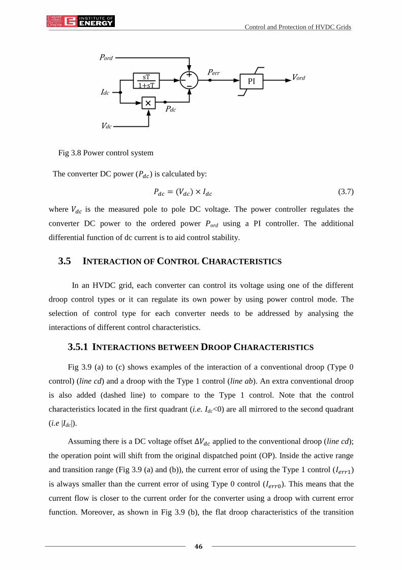
Control and Protection of HVDC Grids
46
Pord
sT
Idc
Vord
Vdc
Perr
Pdc
PI1+sT
Fig 3.8 Power control system
The converter DC power (𝑃𝑑𝑐) is calculated by:
𝑃𝑑𝑐 = (𝑉𝑑𝑐) × 𝐼𝑑𝑐 (3.7)
where 𝑉𝑑𝑐 is the measured pole to pole DC voltage. The power controller regulates the
converter DC power to the ordered power Pord using a PI controller. The additional
differential function of dc current is to aid control stability.
3.5 INTERACTION OF CONTROL CHARACTERISTICS
In an HVDC grid, each converter can control its voltage using one of the different
droop control types or it can regulate its own power by using power control mode. The
selection of control type for each converter needs to be addressed by analysing the
interactions of different control characteristics.
3.5.1 INTERACTIONS BETWEEN DROOP CHARACTERISTICS
Fig 3.9 (a) to (c) shows examples of the interaction of a conventional droop (Type 0
control) (line cd) and a droop with the Type 1 control (line ab). An extra conventional droop
is also added (dashed line) to compare to the Type 1 control. Note that the control
characteristics located in the first quadrant (i.e. Idc<0) are all mirrored to the second quadrant
(i.e |Idc|).
Assuming there is a DC voltage offset ∆𝑉𝑑𝑐 applied to the conventional droop (line cd);
the operation point will shift from the original dispatched point (OP). Inside the active range
and transition range (Fig 3.9 (a) and (b)), the current error of using the Type 1 control (𝐼𝑒𝑟𝑟1)
is always smaller than the current error of using Type 0 control (𝐼𝑒𝑟𝑟0). This means that the
current flow is closer to the current order for the converter using a droop with current error
function. Moreover, as shown in Fig 3.9 (b), the flat droop characteristics of the transition

Control and Protection of HVDC Grids
47
range stabilise the DC voltage, the voltage variation (∆𝑉𝑡𝑟𝑎𝑛𝑠) is very small in this range.
Outside the transition range (Fig 3.9 (c)), the current error function has no effects on the
current flow and the operation point follows the main droop characteristics. Concluding the
above, the Type 1 control has a better current flow control performance than the Type 0
control which has one conventional droop.
|Idc|
Vdc Vdc
Vdc
Ierr0
Ierr1<Ierr0
(a) (b)
(c)
Export: line cd
Import: line ab
∆Vdc ∆Vdc
OP OP
OP
a
b
a
b
a
b
c
d
c
d
c
d
Export: line cd
Import: line ab
∆Vtrans
|Idc|
|Idc|
Ierr1
Ierr0Ierr0
Ierr1<Ierr0
Ierr1<Ierr0
Export: line cd
Import: line ab
∆Vdc
Fig 3.9 Interaction of different droop characteristics in (a): active range; (b): transition
range; and (c) outside the transition range
3.5.2 INTERACTIONS OF POWER AND DROOP CHARACTERISTICS
Fig 3.10 (a) to (b) shows examples of the interaction of a power control curve (curve cd)
and a curve of Type 1 control (red solid line). Assuming there is a power reduction of the
import converter (line cd moves left), the operation point will shift from the original
dispatched point (OP) to its left. In Fig 3.10 (a), the droop controlled converter is exporting
power while the power controller converter is importing power. It can be found the current
error of using a modified current error function (Type 1) is still less than that using
conventional droop control (Type 0) (i.e. 𝐼𝑒𝑟𝑟1 < 𝐼𝑒𝑟𝑟2 ). Conversely, in Fig 3.10 (b), the
power controlled converter is exporting power while the droop controlled converter is
importing power. It can be found 𝐼𝑒𝑟𝑟1 is larger than 𝐼𝑒𝑟𝑟2. The current error function actually
enlarges the current error. This is because the slopes of droop characteristics and the power
curve are of the same sign, the current error sensitivity to voltage offset is actually less for

Control and Protection of HVDC Grids
48
conventional droop characteristics. Therefore, in this case, Type 0 control has a better current
control performance.
Vdc
Ierr1>Ierr0(b)
b
a
d
c
|Idc|
Vdc
(a)
a
d
c
|Idc|
Ierr1Ierr0
bExport: line cd
Import: line abImport: line cd
Export: line ab
Ierr1
Ierr0
Ierr1<Ierr0
OP OP
Fig 3.10 Interaction of droop characteristics and power control characteristics
The current control performance of different methods (within active range) is
summarised in Table 3-4. In an HVDC grid with all converters in Type 0 to Type 2 control,
Type 2 and Type 1 control will have a better current control performance (i.e. less total
current error) than Type 0 control. Their high droop will lead to small current errors. In an
HVDC grid with converters in both Type 0 to Type 2 control and power control, if the sum of
current flowing through power controlled converters is positive (i.e. importing), Type 2 and
Type 1 control will still have a better current control performance. Conversely, if the sum of
current flowing through power controlled converters is negative (i.e. exporting), Type 0
control will still have a better current control performance. This conclusion is further
validated in the Section 3.5.3.
Table 3-4 CURRENT CONTROL PERFORMANCE OF DIFFERENT CONTROL METHODS
Control Types of Converters Method with better current control
performance
All in Type 0 to Type 2 Type 2 and Type 1
Type 0 to Type 2 control, power
control (import) Type 2 and Type 1
Type 0 to Type 2 control, power
control (export) Type 0 control

Control and Protection of HVDC Grids
49
3.5.3 MATHEMATICAL ANALYSIS OF CONTROL INTERACTIONS
In an HVDC grid, converters can have more than one control type. Fig 3.11 shows a
HVDC grid with m converters in power control mode and n converters in alternative droop
control mode (i.e. Type 0 to Type 2).
Power Control
~
~
~ ~
Alternative Droop Control
1
i
m n
DC Grid
Vd
c
+Idc
~j
~1Vdrp1
Vdrpi
Vdrpm
Vpower1
Vpowerj
Vpowern
Idrp1
Idrpi
Idrpm
Ipower1
Ipowerj
Ipowern
Fig 3.11 A HVDC grid of controls in both power and alternative droop control
The current flow change within this generic HVDC grid should be balanced as:
∑∆𝐼𝑑𝑟𝑝𝑖
𝑛
𝑖=1
+∑∆𝐼𝑝𝑜𝑤𝑒𝑟𝑗
𝑚
𝑗=1
= 0 (3.9)
where ∆𝐼𝑑𝑟𝑝𝑖 is the change of measured DC current flowing through a droop controlled
converter and ∆𝐼𝑝𝑜𝑤𝑒𝑟𝑗 is the change of measured DC current flowing through a power
controlled converter.
Normally the converters in droop control will operate in their active region (if any), the
small-signal equation Eq. (3.9) can then be fully extended as:
∑(𝐿𝑅𝑆𝑃𝑖 × ∆𝑃𝑜𝑟𝑑𝑖 + 𝑃𝑜𝑟𝑑𝑖 × ∆𝐿𝑅𝑆𝑃𝑖
𝐿𝑅𝑆𝑃𝑖(𝐿𝑅𝑆𝑃𝑖 + ∆𝐿𝑅𝑆𝑃𝑖))
𝑛
𝑖=1
−∑(1
𝑘𝑖× ∆𝑉𝑑𝑟𝑝𝑖) +
𝑛
𝑖=1
∑(1
𝑘𝑖× ∆𝐿𝑅𝑆𝑃𝑖) +
𝑛
𝑖=1
∑(𝜕𝐼𝑝𝑜𝑤𝑒𝑟𝑗
𝜕𝑉𝑝𝑜𝑤𝑒𝑟𝑗× ∆𝑉𝑝𝑜𝑤𝑒𝑟𝑗 +
𝜕𝐼𝑝𝑜𝑤𝑒𝑟𝑗
𝜕𝑃𝑝𝑜𝑤𝑒𝑟𝑗× ∆𝑃𝑝𝑜𝑤𝑒𝑟𝑗)
𝑚
𝑗=1
= 0 (3.10)
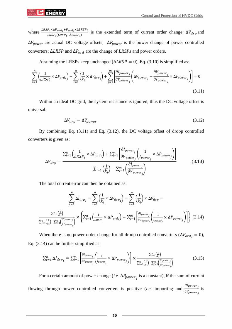
Control and Protection of HVDC Grids
50
where 𝐿𝑅𝑆𝑃𝑖×∆𝑃𝑜𝑟𝑑𝑖+𝑃𝑜𝑟𝑑𝑖×∆𝐿𝑅𝑆𝑃𝑖
𝐿𝑅𝑆𝑃𝑖(𝐿𝑅𝑆𝑃𝑖+∆𝐿𝑅𝑆𝑃𝑖) is the extended term of current order change; ∆𝑉𝑑𝑟𝑝 and
∆𝑉𝑝𝑜𝑤𝑒𝑟 are actual DC voltage offsets; ∆𝑃𝑝𝑜𝑤𝑒𝑟 is the power change of power controlled
converters; ∆𝐿𝑅𝑆𝑃 and ∆𝑃𝑜𝑟𝑑 are the change of LRSPs and power orders.
Assuming the LRSPs keep unchanged (∆𝐿𝑅𝑆𝑃 = 0), Eq. (3.10) is simplified as:
∑(1
𝐿𝑅𝑆𝑃𝑖× ∆𝑃𝑜𝑟𝑑𝑖)
𝑛
𝑖=1
−∑(1
𝑘𝑖× ∆𝑉𝑑𝑟𝑝𝑖) +
𝑛
𝑖=1
∑[𝜕𝐼𝑝𝑜𝑤𝑒𝑟𝑗𝜕𝑉𝑝𝑜𝑤𝑒𝑟𝑗
(∆𝑉𝑝𝑜𝑤𝑒𝑟𝑗 +𝜕𝑉𝑝𝑜𝑤𝑒𝑟𝑗𝜕𝑃𝑝𝑜𝑤𝑒𝑟𝑗
× ∆𝑃𝑝𝑜𝑤𝑒𝑟𝑗)]
𝑚
𝑗=1
= 0
(3.11)
Within an ideal DC grid, the system resistance is ignored, thus the DC voltage offset is
universal:
∆𝑉𝑑𝑟𝑝 = ∆𝑉𝑝𝑜𝑤𝑒𝑟 (3.12)
By combining Eq. (3.11) and Eq. (3.12), the DC voltage offset of droop controlled
converters is given as:
∆𝑉𝑑𝑟𝑝 =
∑ (1
𝐿𝑅𝑆𝑃𝑖× ∆𝑃𝑜𝑟𝑑𝑖)
𝑛𝑖=1 + ∑ [
𝜕𝐼𝑝𝑜𝑤𝑒𝑟𝑗𝜕𝑉𝑝𝑜𝑤𝑒𝑟𝑗
(1
𝐼𝑝𝑜𝑤𝑒𝑟𝑗× ∆𝑃𝑝𝑜𝑤𝑒𝑟𝑗
)]𝑚𝑗=1
∑ (1𝑘𝑖) − ∑ (
𝜕𝐼𝑝𝑜𝑤𝑒𝑟𝑗𝜕𝑉𝑝𝑜𝑤𝑒𝑟𝑗
)𝑚𝑗=1
𝑛𝑖=1
(3.13)
The total current error can then be obtained as:
∑∆𝐼𝑑𝑟𝑝𝑖
𝑛
𝑖=1
=∑(1
𝑘𝑖× ∆𝑉𝑑𝑟𝑝𝑖
) =∑(1
𝑘𝑖)
𝑛
𝑖=1
𝑛
𝑖=1
× ∆𝑉𝑑𝑟𝑝 =
∑ (1
𝑘𝑖)𝑛
𝑖=1
∑ (1
𝑘𝑖)−∑ (
𝜕𝐼𝑝𝑜𝑤𝑒𝑟𝑗
𝜕𝑉𝑝𝑜𝑤𝑒𝑟𝑗
)𝑚𝑗=1
𝑛𝑖=1
× ∑ (1
𝐿𝑅𝑆𝑃𝑖× ∆𝑃𝑜𝑟𝑑𝑖)
𝑛𝑖=1 + ∑ [
𝜕𝐼𝑝𝑜𝑤𝑒𝑟𝑗
𝜕𝑉𝑝𝑜𝑤𝑒𝑟𝑗
(1
𝐼𝑝𝑜𝑤𝑒𝑟𝑗
× ∆𝑃𝑝𝑜𝑤𝑒𝑟𝑗)]𝑚
𝑗=1 (3.14)
When there is no power order change for all droop controlled converters (∆𝑃𝑜𝑟𝑑𝑖 = 0),
Eq. (3.14) can be further simplified as:
∑ ∆𝐼𝑑𝑟𝑝𝑖𝑛𝑖=1 = ∑ [
𝜕𝐼𝑝𝑜𝑤𝑒𝑟𝑗
𝜕𝑉𝑝𝑜𝑤𝑒𝑟𝑗
(1
𝐼𝑝𝑜𝑤𝑒𝑟𝑗
× ∆𝑃𝑝𝑜𝑤𝑒𝑟𝑗)]𝑚
𝑗=1 ×∑ (
1
𝑘𝑖)𝑛
𝑖=1
∑ (1
𝑘𝑖)−∑ (
𝜕𝐼𝑝𝑜𝑤𝑒𝑟𝑗
𝜕𝑉𝑝𝑜𝑤𝑒𝑟𝑗
)𝑚𝑗=1
𝑛𝑖=1
(3.15)
For a certain amount of power change (i.e. ∆𝑃𝑝𝑜𝑤𝑒𝑟𝑗 is a constant), if the sum of current
flowing through power controlled converters is positive (i.e. importing and 𝜕𝐼𝑝𝑜𝑤𝑒𝑟𝑗
𝜕𝑉𝑝𝑜𝑤𝑒𝑟𝑗 is
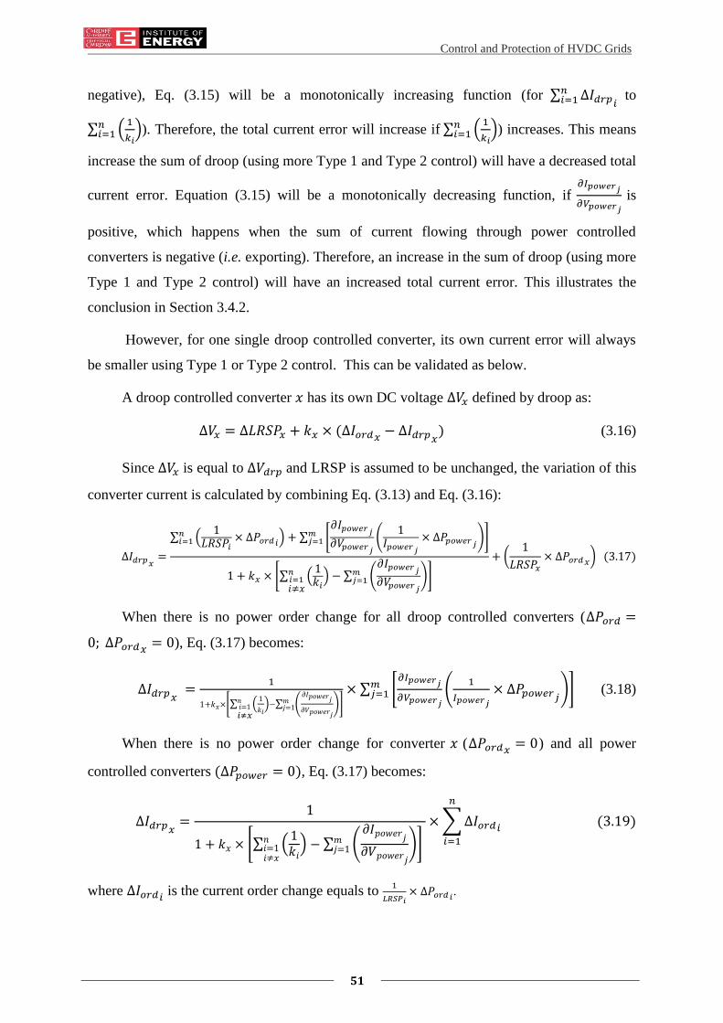
Control and Protection of HVDC Grids
51
negative), Eq. (3.15) will be a monotonically increasing function (for ∑ ∆𝐼𝑑𝑟𝑝𝑖𝑛𝑖=1 to
∑ (1
𝑘𝑖)𝑛
𝑖=1 ). Therefore, the total current error will increase if ∑ (1
𝑘𝑖)𝑛
𝑖=1 ) increases. This means
increase the sum of droop (using more Type 1 and Type 2 control) will have a decreased total
current error. Equation (3.15) will be a monotonically decreasing function, if 𝜕𝐼𝑝𝑜𝑤𝑒𝑟𝑗
𝜕𝑉𝑝𝑜𝑤𝑒𝑟𝑗 is
positive, which happens when the sum of current flowing through power controlled
converters is negative (i.e. exporting). Therefore, an increase in the sum of droop (using more
Type 1 and Type 2 control) will have an increased total current error. This illustrates the
conclusion in Section 3.4.2.
However, for one single droop controlled converter, its own current error will always
be smaller using Type 1 or Type 2 control. This can be validated as below.
A droop controlled converter 𝑥 has its own DC voltage ∆𝑉𝑥 defined by droop as:
∆𝑉𝑥 = ∆𝐿𝑅𝑆𝑃𝑥 + 𝑘𝑥 × (∆𝐼𝑜𝑟𝑑𝑥 − ∆𝐼𝑑𝑟𝑝𝑥) (3.16)
Since ∆𝑉𝑥 is equal to ∆𝑉𝑑𝑟𝑝 and LRSP is assumed to be unchanged, the variation of this
converter current is calculated by combining Eq. (3.13) and Eq. (3.16):
∆𝐼𝑑𝑟𝑝𝑥 =
∑ (1
𝐿𝑅𝑆𝑃𝑖× ∆𝑃𝑜𝑟𝑑𝑖)
𝑛𝑖=1 + ∑ [
𝜕𝐼𝑝𝑜𝑤𝑒𝑟𝑗𝜕𝑉𝑝𝑜𝑤𝑒𝑟𝑗
(1
𝐼𝑝𝑜𝑤𝑒𝑟𝑗× ∆𝑃𝑝𝑜𝑤𝑒𝑟𝑗)]
𝑚𝑗=1
1 + 𝑘𝑥 × [∑ (1𝑘𝑖) − ∑ (
𝜕𝐼𝑝𝑜𝑤𝑒𝑟𝑗𝜕𝑉𝑝𝑜𝑤𝑒𝑟𝑗
)𝑚𝑗=1
𝑛𝑖=1𝑖≠𝑥
]
+ (1
𝐿𝑅𝑆𝑃𝑥× ∆𝑃𝑜𝑟𝑑𝑥) (3.17)
When there is no power order change for all droop controlled converters (∆𝑃𝑜𝑟𝑑 =
0; ∆𝑃𝑜𝑟𝑑𝑥 = 0), Eq. (3.17) becomes:
∆𝐼𝑑𝑟𝑝𝑥 =1
1+𝑘𝑥×[∑ (1
𝑘𝑖)−∑ (
𝜕𝐼𝑝𝑜𝑤𝑒𝑟𝑗
𝜕𝑉𝑝𝑜𝑤𝑒𝑟𝑗
)𝑚𝑗=1
𝑛𝑖=1𝑖≠𝑥
]
× ∑ [𝜕𝐼𝑝𝑜𝑤𝑒𝑟𝑗
𝜕𝑉𝑝𝑜𝑤𝑒𝑟𝑗(
1
𝐼𝑝𝑜𝑤𝑒𝑟𝑗× ∆𝑃𝑝𝑜𝑤𝑒𝑟𝑗)]
𝑚𝑗=1 (3.18)
When there is no power order change for converter 𝑥 (∆𝑃𝑜𝑟𝑑𝑥 = 0) and all power
controlled converters (∆𝑃𝑝𝑜𝑤𝑒𝑟 = 0), Eq. (3.17) becomes:
∆𝐼𝑑𝑟𝑝𝑥 =1
1 + 𝑘𝑥 × [∑ (1𝑘𝑖) − ∑ (
𝜕𝐼𝑝𝑜𝑤𝑒𝑟𝑗𝜕𝑉𝑝𝑜𝑤𝑒𝑟𝑗
)𝑚𝑗=1
𝑛𝑖=1𝑖≠𝑥
]
×∑∆𝐼𝑜𝑟𝑑𝑖
𝑛
𝑖=1
(3.19)
where ∆𝐼𝑜𝑟𝑑𝑖 is the current order change equals to 1
𝐿𝑅𝑆𝑃𝑖× ∆𝑃𝑜𝑟𝑑𝑖.

Control and Protection of HVDC Grids
52
If there are only droop controlled converters, Eq. (3.19) can even be further simplified
as:
∆𝐼𝑑𝑐𝑥 =1
1 + 𝑘𝑥 × ∑ (1𝑘𝑖)𝑛
𝑖=1𝑖≠𝑥
×∑∆𝐼𝑜𝑟𝑑𝑖
𝑛
𝑖=1
(3.20)
Equation (3.18) to Eq. (3.20) show that a higher value of droop (i.e. 𝑘𝑥) will always
make its converter current less sensitive to the power order change of all the other converters.
3.6 MULTIPLE CROSS-OVER OF CONTROL CHARACTERISTICS
The use of both power control and Type 1 or Type 2 control in a HVDC grid will have
possible adverse interactions of control characteristics. This happens between exporting
station(s) in power control with an importing station(s) in Type 1 and Type 2 control. Under
this operating mode a condition could exist where the relative slope of the two characteristics
could give rise to more than one possible operating point (See Fig 3.12 (a)). Furthermore,
transitions between the operating points would occur for relatively minor changes in
operation of the grid. These transitions manifest themselves as incorrect operating points for
the scheme and potentially undesirable and unpredictable changes in the DC currents and
voltages within the DC grid. This condition can only exist if the gradient of the high droop
section of the characteristics is greater than that of the constant power characteristics. It
should be emphasised that these characteristics are not necessarily those of individual
converters but the combined effect of all of the converters in the DC grid.
A further complication can arise during power ramps where any delay in the control
systems (i.e. the power controller) will result in a transient error between the power orders to
the power control and droop control converter(s). This is illustrated in Fig 3.12 (b) and Fig
3.12 (c). For example a rising power order may cause the operating point to be at OP1 (Fig
3.12 (b)); once the power ramp is complete the operating point would move to OP2, which is
unstable. Operation would then move to either OP1 or OP3.

Control and Protection of HVDC Grids
53
Fig 3.12 a) Multiple Operating Points, b) Reduced Power, c) Increased Power
A similar situation can exist for power reductions where operation will be at OP3 during
the power ramp as, again, the power controlling converter(s) will lag behind that of the droop
controlled converter(s).
In order to avoid any ambiguity of the operating point, the value of high droop should
be smaller than the smallest slope of the constant power curve within the active range (Note
slope of power curve varies with current change). Fig 3.13 gives an example of a droop
characteristic with a small active range (red) cross-over and a power curve (green).
Vdc
+Idc
∂Vpower
Vdc
+Idc
∂Ipower >k∂Vpower
∂Ipower >k
(a) (b)
Fig 3.13 Multiple operating points
Converter A (Import)
Droop Characteristic
Converter B (Export)
Constant Power Characteristic
LRSP
Vdc
Idc
OP3
(c)
OP3
OP1
Converter B (Export)
Constant Power Characteristic
OP1
OP2
OP3
(a)
OP2
OP3
Converter A (Import)
Droop Characteristic
Converter B (Export)
Constant Power Characteristic
LRSP
Vdc
Idc
OP1
(b)
Converter A (Import)
Droop Characteristic OP1
Vdc
Idc
OP2 OP2

Control and Protection of HVDC Grids
54
Within the band, if the droop ( 𝑘 ) is larger than the slope of power curve |𝜕𝑉𝑝𝑜𝑤𝑒𝑟
𝜕𝐼𝑝𝑜𝑤𝑒𝑟|
(Fig 3.13 a), there can be three different operation points while if the 𝑘 is smaller than
the |𝜕𝑉𝑝𝑜𝑤𝑒𝑟
𝜕𝐼𝑝𝑜𝑤𝑒𝑟| (Fig 3.13 b), there can only be one operation point.
Essentially, within a small (current) region, the power curve is almost linear, while the
droop control characteristics are non-linear due to the difference between the slope inside and
outside the active range. This non-linearity gives the potential a risk of multiple curve
crossing. When the value of droop inside the band is larger than the slope of power curve,
but conversely smaller outside the band, these two curves can have one crossing within the
band, and two crossing outside the band.
To avoid the multiple operating points the maximum allowable value for the high droop
setting can be estimated by the following analysis.
Within the example HVDC grid as shown in Fig 3.11, the sum of current flowing
through converters is balanced:
∑𝐼𝑑𝑟𝑝𝑖
𝑛
𝑖=1
+∑𝐼𝑝𝑜𝑤𝑒𝑟𝑗
𝑚
𝑗=1
= 0 (3.21)
where 𝐼𝑑𝑟𝑝𝑖 is the current of one droop controlled converter while 𝐼𝑝𝑜𝑤𝑒𝑟𝑗 is the current of
one power controlled converter.
Normally the converters in droop control will operate in their active region (if any)
which gives:
𝐼𝑑𝑟𝑝𝑖 = 𝐼𝑜𝑟𝑑𝑖 −1
𝑘𝑖× 𝑉𝑑𝑟𝑝𝑖 +
(1
𝑘𝑖× 𝐿𝑅𝑆𝑃𝑖) (3.22)
Currents of converters in power control can be calculated as:
𝐼𝑝𝑜𝑤𝑒𝑟𝑗 =𝑃𝑝𝑜𝑤𝑒𝑟𝑗
𝑉𝑝𝑜𝑤𝑒𝑟𝑗 (3.23)
Substituting Eq. (3.22) and Eq. (3.23) into Eq. (3.21) gives:
∑(𝐼𝑜𝑟𝑑𝑖)
𝑛
𝑖=1
−∑(1
𝑘𝑖× 𝑉𝑑𝑟𝑝𝑖) +
𝑛
𝑖=1
∑(1
𝑘𝑖× 𝐿𝑅𝑆𝑃𝑖) +∑(
𝑃𝑝𝑜𝑤𝑒𝑟𝑗
𝑉𝑝𝑜𝑤𝑒𝑟𝑗 )
𝑚
𝑗=1
= 0 (3.24)
𝑛
𝑖=1
where 𝑉𝑑𝑟𝑝𝑖 and 𝑉𝑝𝑜𝑤𝑒𝑟𝑗are the measured voltages of droop controlled converters and power
controlled converters.
Control and Protection of HVDC Grids
55
For simplicity, assuming all droop controlled converters have the same LRSP, and all
power converters maintain constant power (𝑉𝑑𝑟𝑝 = 𝑉𝑑𝑟𝑝𝑖 = 𝑉𝑝𝑜𝑤𝑒𝑟𝑗). To find slopes of the
equivalent control characteristics of all converters in power control and all converter in droop
control the derivative of Eq. (3.24) can be taken with respect to voltage (Vdrp):
-∑ (1
𝑘𝑖)𝑛
𝑖=1 + ∑ (𝑃𝑜𝑟𝑑𝑒𝑟𝑗
𝐿𝑅𝑆𝑃2)𝑚
𝑗=1 = 0 (3.25)
From Eq. (3.25), the term 1 ∑ (1
𝑘𝑖)𝑛
𝑖=1⁄ can be considered as the droop gain of the
merged droop control curve and 1 ∑ (𝑃𝑜𝑟𝑑𝑒𝑟𝑗
𝐿𝑅𝑆𝑃2)𝑚
𝑗=1⁄ can be considered as the slope of the
merged power curve. Both terms (i.e. 1 ∑ (1
𝑘𝑖)𝑛
𝑖=1⁄ and 1 ∑ (𝑃𝑜𝑟𝑑𝑒𝑟𝑗
𝐿𝑅𝑆𝑃2)𝑚
𝑗=1⁄ ) reflect the DC
voltage response of changing the current through all the droop controlled converters and the
power controlled converters.
Equation (3.26) should then be satisfied to avoid multiple curve crossing:
|1∑ (
1
𝑘𝑖)𝑛
𝑖=1⁄ |
≤|1∑ (
𝑃𝑜𝑟𝑑𝑒𝑟𝑗
𝐿𝑅𝑆𝑃2)𝑚
𝑗=1⁄ |
(3.26)
From Eq. (3.26), it can be concluded that:
In an ideal DC grid, multiple operation points can only exist when there is at least one
export converter in power control and the sum of current flowing through power
controlled converters should be negative (i.e. export).
Higher absolute values of 1
∑ (1
𝑘𝑖)𝑛
𝑖=1
are more likely to cause multiple operation points.
Therefore, equation (3.26) should always be satisfied in order to guarantee the stable
operating within the active region. The boundary condition will be when the slope of
the droop characteristics is equal to the tangential slope of the power
characteristics |1∑ (
1
𝑘𝑖)𝑛
𝑖=1⁄ |
=|1∑ (
𝑃𝑜𝑟𝑑𝑒𝑟𝑗
𝐿𝑅𝑆𝑃2)𝑚
𝑗=1⁄ |
.
Control and Protection of HVDC Grids
56
The increase of LRSP can allow higher droop gain to be selected.
The decrease of sum of power orders ∑ (𝑃𝑜𝑟𝑑𝑗)𝑛𝑗=1 allows higher droop gain to be
selected
3.7 SUMMARY
This chapter discusses the use of alternative droop characteristics to control a HVDC
grid. The conventional droop characteristics (Type 0 control) have been further developed to
include a current error function with only active range (Type 2 control) and with both active
range and transition range (Type 1 control).
The control algorithm and mathematic expressions of different droop characteristics are
given. Analysis of interactions of converter control characteristics has been undertaken to
compare the control performance of different control types applied in an HVDC grid. Proper
use of alternative droops can increase the accuracy of DC current flow control while stabilise
the DC voltage during large power disturbance. The analysis shows that in an HVDC grid in
which most export converters are in power control mode, the use of Type 0 control in the
other converters is better for current flow control (i.e. less total current error). However, if
most import converters are in power control mode, Type 1 and 2 control are better for current
flow regulation. This has also been mathematically illustrated.
It has also been found that the use of higher droop gain on one converter will lead to
less DC current offset of this particular converter.
Moreover, multiple cross-over of control characteristics can exist when Type 2 or Type
1 control used for import converters and power control used for export converters. The
multiple operation points can lead the DC system to operate at different voltage levels while
power flow is unchanged. A method of designing the range of droop has been provided to
avoid multiple operation points.
The control of HVDC grids using alternative droop characteristics has been
demonstrated using both a HVDC test rig and PSCAD/EMTDC. This will be presented in
Chapter 4 in detail and the simulation results will also be given.
Control and Protection of HVDC Grids
57
Chapter 4
4. Computer Simulation and
experimental Validation of ACC
4.1 INTRODUCTION
The Autonomous Converter Control (ACC) designed in Chapter 3 was tested using a
physical 4-terminal HVDC test rig associated with the main AC power supply. This chapter
aims to show the physical implementation of ACC and the effectiveness of using different
droop characteristics (e.g. Type 2 control or Type 1 control) to reduce the current error of
converters. The test rig was also used to demonstrate the effects of multiple cross-overs in the
static characteristics. Moreover, digital simulation using PSCAD/EMTDC were also
performed and the results obtained were compared with the experimental results.
4.2 CONFIGURATION OF 4-TERMINAL HVDC TEST RIG
A 4-terminal HVDC test rig has been configured as shown in Fig 4.1 where the ACC
was implemented. This rig consists of three 2-level VSCs in one cabinet, a fourth 2-level
VSC in an individual cabinet, three transformers, two motor-generator units with Unidrives
and a Human-Machine Interface (HMI).
3 VSCs
Transformers
Unidrive
Fourth VSC
HMI
Motor- Generator
Units
Fig 4.1 Configuration of the 4-terminal HVDC test rig
Fig 4.2 (a) shows the view inside the cabinet of three VSCs. The VSCs are integrated
on three Printed Circuit Boards (PCBs) associated with inductors at both their AC and DC

Control and Protection of HVDC Grids
58
sides. The AC inductors are phase reactors rated at 2.4 mH (i.e. 0.3 p.u) which are used to
control the power flow and filter high frequency components generated by IGBT switching.
The DC inductors are converter reactors (also rated at 2.4 mH) which smooth DC current.
These VSCs are controlled by the dSPACE control unit.
The fourth VSC in the individual cabinet has the same physical configuration whilst is
controlled by a Digital Signal Processor (DSP).
Fig 4.2 (b) gives a clearer view of an individual PCB. This PCB consists of two sub-
PCBs. The upper sub-PCB includes Six-Pack IGBT Modules (MiniSKiiP®) driven by the 6-
channel divers (SKHI 61 (R)), a protection circuit and the control interface to transmit
analogue signals between VSCs and the dSPACE control unit. The sub-PCB underneath
includes a DC capacitor bank (rated at 1020 uF for smoothing DC voltage), DC nodes
connecting to the DC inductors, AC nodes connecting to the AC inductors, LEM DC voltage
sensors and both LEM AC and DC current sensors.
dSPACE
DC inductors
AC inductors
Sixpack IGBTs and
driver
VSCs
Capacitor bank
Protection circuit
Control interface
AC nodes
DC nodes
Sensorsunderneath
Fig 4.2 Physical model of VSCs (a): inside view of cabinet of VSCs; (b) PCBs
The inside view of Unidrives is given in Fig 4.3. These two Unidrives (i.e. Undrive
SP Size 2 (5.5 to 15 kW)) are used to drive the motor-generator units (back-back permanent
magnet synchronous machines). The control signals for motor-generator units (e.g. torque

Control and Protection of HVDC Grids
59
control order or speed control order) are also sent by the dSPACE control unit via the
Universal Signal Transmitter 4114 to the Unidrives and thus regulate the motor-generator
units.
Fig 4.3 Inside view of cabinet containing Unidrives
The HMI is the workspace for the operator controlling the test rig. An operator can
use the HMI to send control orders (e.g. power order, voltage order) to each VSC and
Unidrive to control the system operating. (More details are given in Section 4.4).
These four VSCs (shown in Fig 4.1) can then be connected using the physical
representations of DC cables shown in Fig 4.4 which are composed of multiple π sections.
The inductance and capacitance of each π section are selected to represent a segment of a
scaled-down cable model with its characteristic impedance (𝑍𝑜) and propagation velocity (𝛾)
equalling to the typical values (i.e. 𝑍𝑜 = 40 Ω; 𝛾= 54% of speed of light [75], [76]). The
inductors also provide equivalent resistance for this DC transmission line model.
There are multiple accessible points for inserting different number of π sections into
circuits thus to represent different length of cables. Moreover, these accessible points provide
flexibility for configuring different DC system topologies (e.g. the DC side can be connected
as either a radial connection or a meshed grid).

Control and Protection of HVDC Grids
60
0.5 mH
0.5 mH
20
0 u
F
20
0 u
F
20
0 u
F
20
0 u
F
20
0 u
F
20
0 u
F
20
0 u
F
20
0 u
F
20
0 u
F
20
0 u
F
20
0 u
F
20
0 u
F
I_dc5a
I_dc5b
I_dc7b
I_dc7a
I_dc6a
I_dc6b
0.5 mH 0.5 mH 0.5 mH
0.5 mH 0.5 mH 0.5 mH 0.5 mH
0.5 mH
0.5 mH0.5 mH 0.5 mH 0.5 mH 0.5 mH
0.5 mH0.5 mH0.5 mH
20
0 u
F
20
0 u
F
20
0 u
F
20
0 u
F
20
0 u
F
20
0 u
F
0.5 mH
0.5 mH
20
0 u
F
20
0 u
F
20
0 u
F
20
0 u
F
20
0 u
F
0.5 mH
20
0 u
F
20
0 u
F
20
0 u
F
20
0 u
F
20
0 u
F
I_dc8b
I_dc8a
0.5 mH 0.5 mH 0.5 mH
0.5 mH 0.5 mH 0.5 mH 0.5 mH2
00
uF
20
0 u
F
20
0 u
F
20
0 u
F
20
0 u
F
20
0 u
F
0.5 mH
0.5 mH
20
0 u
F
20
0 u
F
20
0 u
F
20
0 u
F
Fig 4.4 Cable representations: (a) DC cable model (b) Physical representations
4.3 SYSTEM CONFIGURATION FOR TESTING ACC
The ACC control method proposed in Chapter 3 was then tested on this 4-terminal
HVDC test rig connected in a star-configuration.
M GUnidrive
Motor to
emulatePMSG
Mechanical
Conection
DC
network
~
~
dSPACEGS1
GS2
WF2
Optic
link
R3
R4
R2
MATLAB/SIMULINK,ControlDesk
M G
Motor to
emulatePMSG
Mechanical
ConectionUnidrive
WF1
dsp
CAN-
communication
Telecommunication
R1
WF1
WF2
GS2
GS1Cgs1
Lwf1
Lwf2
Lgs2
Lgs1
Cgs2
Cwf1
Cwf2
L1 R1
L2 R2
L3 R3
L4 R4
(a) (b)
DC
cable
model
Fig 4.5 Star-connected VSC simulator: (a) Circuit diagram; (b) Simulator set-up
The circuit diagram is shown in Fig 4.5 (a). Two VSCs connected with two WFs are
named as WF1 and WF2 while others are connected with two onshore AC grids named as

Control and Protection of HVDC Grids
61
GS1 and GS2. Fig 4.5 (b) shows the HVDC test rig set-up to approach the circuit depicted in
Fig 4.5 (a). The HVDC test rig uses autotransformers connecting the laboratory 415 V AC
power supply to represent two onshore AC grid connection points and the motor-generator
units are used to represent offshore wind farms. The motor-generator units are then connected
to the DC links through the converters WF1 and WF2 to emulate the operation of offshore
windfarm connected with a HVDC grid.
The specifications for the simulation using the HVDC test rig are given in Table 4-1.
For comparison, digital simulations using PSCAD/EMTDC were also undertaken on the
same system in Fig 4.5 (a) whilst used the scaled-up data given in Table 4-1.
Table 4-1 SUMMARY OF SIMULATION PARAMETERS
Devices Initial control setting and
physical parameter
Physical model PSCAD model
Voltage
Source
Converters
Power Order 500 W 500 MW
Slope of main droop 6.25 V/A 6.25 kV/kA
LRSP 250 V 250 kV
Topology Two-level, three
phase, without
neutral wire
Simplified
converter model
[77]
Wind farm
(Motor-
Generator
Unit)
Rated power 1 kW 1 GW
Rated voltage (L-L rms) 145 V 145 kV
AC inductors Lgs1, Lgs2, Lwf1, Lwf1 2.2 mH
DC resistors R1, R3 0.15 Ω
R2 0.07 Ω
R4 0.17 Ω
DC capacitors Cgs1, Cgs2, Cwf1, Cwf1 1020 μF
Note that the VSC model used for the digital simulations is a simplified converter
model as shown in Fig 4.6. It consists of both a controllable DC voltage supply and a fixed
DC voltage supply.
During normal operation, the VSC acts as a controllable voltage source regulating the
DC voltage dictated by the selected modulation index. The modulation index can be
generated by the using the ACC controller that developed in Chapter 3. The fixed DC voltage
supply is added for DC fault study. During a DC fault, a converter will block and conduct in
an uncontrolled manner. The current will then follow through the freewheel diode.
More details regarding to the VSC are given in [77].
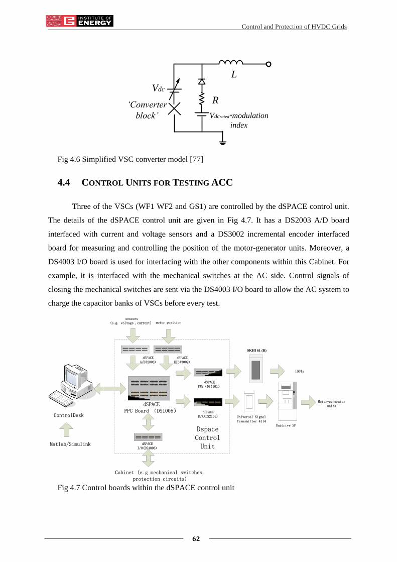
Control and Protection of HVDC Grids
62
Vdc
‘Converter
block’
R
Vdcrated*modulation
index
L
Fig 4.6 Simplified VSC converter model [77]
4.4 CONTROL UNITS FOR TESTING ACC
Three of the VSCs (WF1 WF2 and GS1) are controlled by the dSPACE control unit.
The details of the dSPACE control unit are given in Fig 4.7. It has a DS2003 A/D board
interfaced with current and voltage sensors and a DS3002 incremental encoder interfaced
board for measuring and controlling the position of the motor-generator units. Moreover, a
DS4003 I/O board is used for interfacing with the other components within this Cabinet. For
example, it is interfaced with the mechanical switches at the AC side. Control signals of
closing the mechanical switches are sent via the DS4003 I/O board to allow the AC system to
charge the capacitor banks of VSCs before every test.
dSPACE D/A(DS2103) Universal Signal
Transmitter 4114Unidrive SP
dSPACE PWM(DS5101)
dSPACE PPC Board (DS1005)
SKHI 61 (R)
dSPACE A/D(2003)
sensors (e.g. voltage ,current)
dSPACE I/O(DS4003)
ControlDesk
Motor-generator units
IGBTs
Matlab/Simulink
DspaceControlUnit
Cabinet (e.g mechanical switches, protection circuits)
motor position
dSPACE EIB(3002)
Fig 4.7 Control boards within the dSPACE control unit
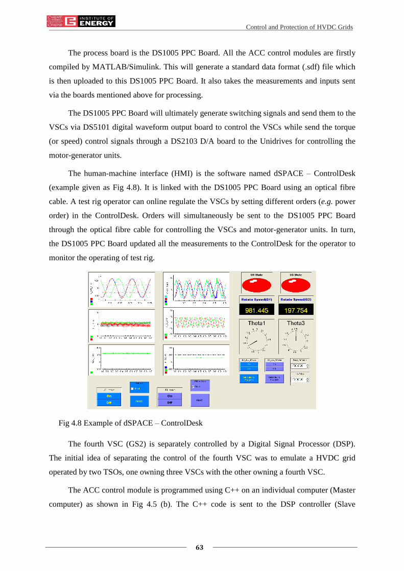
Control and Protection of HVDC Grids
63
The process board is the DS1005 PPC Board. All the ACC control modules are firstly
compiled by MATLAB/Simulink. This will generate a standard data format (.sdf) file which
is then uploaded to this DS1005 PPC Board. It also takes the measurements and inputs sent
via the boards mentioned above for processing.
The DS1005 PPC Board will ultimately generate switching signals and send them to the
VSCs via DS5101 digital waveform output board to control the VSCs while send the torque
(or speed) control signals through a DS2103 D/A board to the Unidrives for controlling the
motor-generator units.
The human-machine interface (HMI) is the software named dSPACE – ControlDesk
(example given as Fig 4.8). It is linked with the DS1005 PPC Board using an optical fibre
cable. A test rig operator can online regulate the VSCs by setting different orders (e.g. power
order) in the ControlDesk. Orders will simultaneously be sent to the DS1005 PPC Board
through the optical fibre cable for controlling the VSCs and motor-generator units. In turn,
the DS1005 PPC Board updated all the measurements to the ControlDesk for the operator to
monitor the operating of test rig.
Fig 4.8 Example of dSPACE – ControlDesk
The fourth VSC (GS2) is separately controlled by a Digital Signal Processor (DSP).
The initial idea of separating the control of the fourth VSC was to emulate a HVDC grid
operated by two TSOs, one owning three VSCs with the other owning a fourth VSC.
The ACC control module is programmed using C++ on an individual computer (Master
computer) as shown in Fig 4.5 (b). The C++ code is sent to the DSP controller (Slave

Control and Protection of HVDC Grids
64
computer) using the Controller Area Network (CAN). The control signal generated by DSP
controller is sent to the fourth VSC for IGBTs switching through an optical fibre cable.
The on-line control and status monitoring of the fourth VSC is via a self-built Graphical
User Interface (GUI) (See Fig 4.9) created using the Microsoft Foundation Class (MFC)
Library. A test rig operator sets control orders and select different types of control methods
for the fourth VSC using this self-built GUI.
Fig 4.9 Self-built Graphical User Interface
4.5 IMPLEMENTATION OF CONVERTER CONTROL WITHIN ACC
The implementation of the converter control within ACC is shown in Fig 4.10.
Within the outer loop control, different control characteristics can be implemented, for
example, the autonomous DC voltage droop control could be selected for an onshore
converter while AC frequency control can be selected for an offshore converter. In addition
the converters can either control the AC voltage or reactive power.
The outer loop control generates the dq0 frame current references (𝐼𝑑∗ , 𝐼𝑞
∗) which are
sent to the Inner loop control (i.e. decoupled current control) . In turn, inner loop control acts
to output a reference value of the converter AC voltage ( 𝑈𝐶_𝑟𝑒𝑓).
The generated control signals are sent to the firing control block to create converter
switching signals.
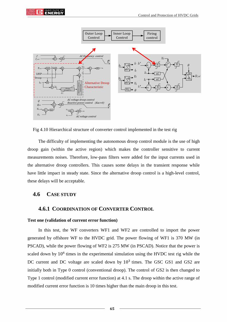
Control and Protection of HVDC Grids
65
Fig 4.10 Hierarchical structure of converter control implemented in the test rig
The difficulty of implementing the autonomous droop control module is the use of high
droop gain (within the active region) which makes the controller sensitive to current
measurements noises. Therefore, low-pass filters were added for the input currents used in
the alternative droop controllers. This causes some delays in the transient response while
have little impact in steady state. Since the alternative droop control is a high-level control,
these delays will be acceptable.
4.6 CASE STUDY
4.6.1 COORDINATION OF CONVERTER CONTROL
Test one (validation of current error function)
In this test, the WF converters WF1 and WF2 are controlled to import the power
generated by offshore WF to the HVDC grid. The power flowing of WF1 is 370 MW (in
PSCAD), while the power flowing of WF2 is 275 MW (in PSCAD). Notice that the power is
scaled down by 106 times in the experimental simulation using the HVDC test rig while the
DC current and DC voltage are scaled down by 103 times. The GSC GS1 and GS2 are
initially both in Type 0 control (conventional droop). The control of GS2 is then changed to
Type 1 control (modified current error function) at 4.1 s. The droop within the active range of
modified current error function is 10 times higher than the main droop in this test.
LRSP
PI Pord N/DIord
Droop
Idc
Ierr
Sele
ctio
n o
f D
roo
p
Co
ntr
ol T
ype
Vord
Vdc
Vac
Vac_ord
PI
Q
kac
Qord
PI
Vac
Vac_ref
AC voltage control
AC voltage droop controlReactive power control (Kac=0)
Alternative Droop
Characteristic
f_ord
fPI
AC frequency control
Id*
Iq*
(Droop-DroopH)*Ierr
Ir1
-Ir1
Outer Loop Control
Inner Loop Control
Firing control
Id
Iq
PI
PI
PI
PI
ωL
ωL
abc
dqIacId
Iq
abc
dqUC_ref
abc
dqVacVd
Vq
PLL Ɵ
Ɵ
Vd
Id *
Iq*
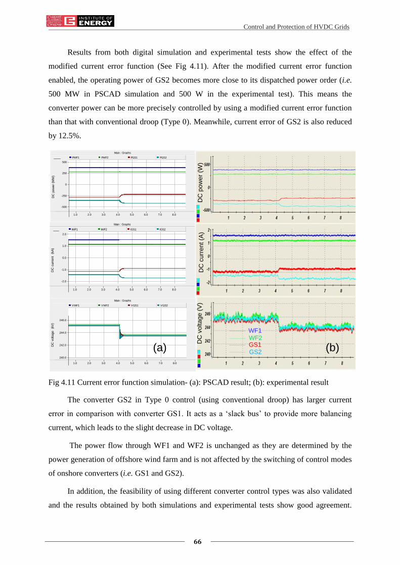
Control and Protection of HVDC Grids
66
Results from both digital simulation and experimental tests show the effect of the
modified current error function (See Fig 4.11). After the modified current error function
enabled, the operating power of GS2 becomes more close to its dispatched power order (i.e.
500 MW in PSCAD simulation and 500 W in the experimental test). This means the
converter power can be more precisely controlled by using a modified current error function
than that with conventional droop (Type 0). Meanwhile, current error of GS2 is also reduced
by 12.5%.
Main : Graphs
1.0 2.0 3.0 4.0 5.0 6.0 7.0 8.0 ...
...
...
-500
-250
0
250
500
DC
pow
er
(MW
)
PWF1 PWF2 PGS1 PGS2
Main : Graphs
1.0 2.0 3.0 4.0 5.0 6.0 7.0 8.0 ...
...
...
-2.0
-1.0
0.0
1.0
2.0
DC
curr
ent
(kA
)
IWF1 IWF2 IGS1 IGS2
Main : Graphs
1.0 2.0 3.0 4.0 5.0 6.0 7.0 8.0 ...
...
...
240.0
242.0
244.0
246.0
DC
voltage
(kV
)
VWF1 VWF2 VGS1 VGS2
(a) (b)
WF1WF2GS1GS2
DC
po
we
r (W
)D
C c
urr
en
t (A
)D
C v
olta
ge
(V
)
Fig 4.11 Current error function simulation- (a): PSCAD result; (b): experimental result
The converter GS2 in Type 0 control (using conventional droop) has larger current
error in comparison with converter GS1. It acts as a ‘slack bus’ to provide more balancing
current, which leads to the slight decrease in DC voltage.
The power flow through WF1 and WF2 is unchanged as they are determined by the
power generation of offshore wind farm and is not affected by the switching of control modes
of onshore converters (i.e. GS1 and GS2).
In addition, the feasibility of using different converter control types was also validated
and the results obtained by both simulations and experimental tests show good agreement.
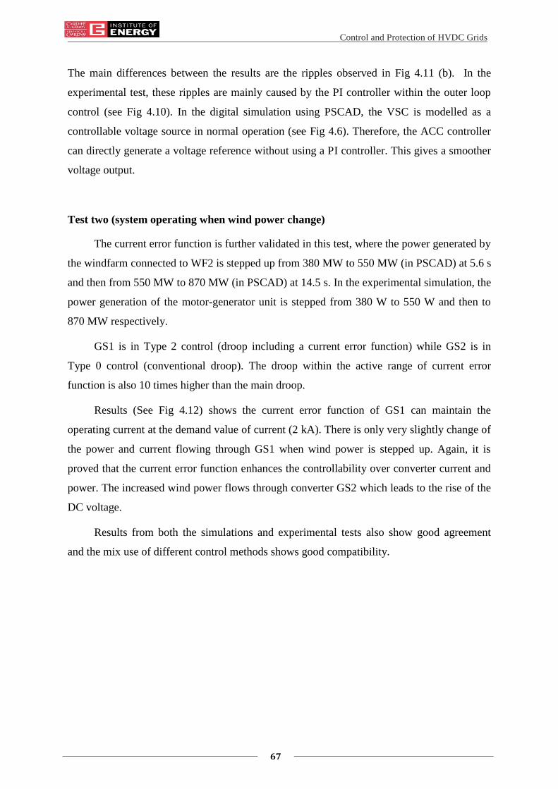
Control and Protection of HVDC Grids
67
The main differences between the results are the ripples observed in Fig 4.11 (b). In the
experimental test, these ripples are mainly caused by the PI controller within the outer loop
control (see Fig 4.10). In the digital simulation using PSCAD, the VSC is modelled as a
controllable voltage source in normal operation (see Fig 4.6). Therefore, the ACC controller
can directly generate a voltage reference without using a PI controller. This gives a smoother
voltage output.
Test two (system operating when wind power change)
The current error function is further validated in this test, where the power generated by
the windfarm connected to WF2 is stepped up from 380 MW to 550 MW (in PSCAD) at 5.6 s
and then from 550 MW to 870 MW (in PSCAD) at 14.5 s. In the experimental simulation, the
power generation of the motor-generator unit is stepped from 380 W to 550 W and then to
870 MW respectively.
GS1 is in Type 2 control (droop including a current error function) while GS2 is in
Type 0 control (conventional droop). The droop within the active range of current error
function is also 10 times higher than the main droop.
Results (See Fig 4.12) shows the current error function of GS1 can maintain the
operating current at the demand value of current (2 kA). There is only very slightly change of
the power and current flowing through GS1 when wind power is stepped up. Again, it is
proved that the current error function enhances the controllability over converter current and
power. The increased wind power flows through converter GS2 which leads to the rise of the
DC voltage.
Results from both the simulations and experimental tests also show good agreement
and the mix use of different control methods shows good compatibility.

Control and Protection of HVDC Grids
68
Main : Graphs
4.0 6.0 8.0 10.0 12.0 14.0 16.0 ...
...
...
240.0
245.0
250.0
255.0
DC
voltage
(kV
)
VWF1 VWF2 VGS1 VGS2
Main : Graphs
4.0 6.0 8.0 10.0 12.0 14.0 16.0 ...
...
...
-1.0k
-0.5k
0.0
0.5k
1.0k
DC
pow
er
(MW
)
PWF1 PWF2 PGS1 PGS2
Main : Graphs
4.0 6.0 8.0 10.0 12.0 14.0 16.0 ...
...
...
-2.0
0.0
2.0
4.0
DC
curr
ent
(kA
)
IWF1 IWF2 IGS1 IGS2
WF1WF2GS1GS2
DC
po
we
r (W
)D
C c
urr
en
t (A
)D
C v
olta
ge
(V
)
(a) (b)
Fig 4.12 Converter operation during change of power condition - (a): PSCAD result; (b):
experimental result

Control and Protection of HVDC Grids
69
4.6.2 MULTIPLE CROSS-OVERS IN THE STATIC CHARACTERISTICS
This section aims to verify the effects of multiple cross-overs in the static
characteristics as shown in Section 3.5. Again both digital simulation using PSCAD and
experiment test using the HVDC test rig are performed for the validation and comparison.
Test one (Digital Simulation Results)
The following figures are from the digital simulation (PSCAD) of the four terminal DC
systems (Fig 4.5 (a)). To show the multiple-crossover characteristics, there must be at least
one converter (importing power to DC grid) using alternative droop control (i.e. Type 1 or
Type 2) and one converter (exporting) in power control mode. Therefore, in this test, two
converters are in Droop (importing) or Constant Power (exporting) control whilst the other
two of the converters control their power to zero.
Basic data of these two converters in Droop control and Constant power control are
given in Table
Table 4-2 BASIC DATA OF CONVERTER CONTROL FOR TEST ONE
Item Parameter
Rating 1.5 GW, 400 kV (± 200 kVdc) @ 3.75 kAdc
Each DC cable resistance 0.15 ohm
Power ramp 0 MW to -1500 MW in 1 second
Import converter (GS1)
Droop Control –
Outside Active region = -5%
Inside Active region = -125%
Active region(Vdc) = ±4%
Export converter (GS2) Constant Pdc Control
Fig 4.13 (a) shows a power ramp with the import converter with a conventional droop
(Type 0 control). As both converters have the same power order (zero communications delay)
it would be expected that the DC voltage would remain at the ordered LRSP of 400 kV
however a combination of a lag introduced by the power control loop and the effect of the
changing DC current on the system inductances gives a small change in the DC voltage (≈ 2

Control and Protection of HVDC Grids
70
kVdc). Once the power ramp is completed the DC voltage returns to its LRSP (400 kVdc). This
means the operating point always locates at OP2 (the desired operating point) in steady state.
Fig 4.13 (a) PSCAD: conventional droop characteristics (power ramp 0 MW to 1500 MW)
Fig 4.13 (b) PSCAD: alternative droop characteristics (power ramp 0 MW to 1500 MW)
Fig 4.13 (c) PSCAD: alternative droop characteristics (power ramp 0 MW to -1500 MW)
-2k
0
2kP
ow
er
(MW
)
380390400410
DC
voltage
(kV
)
VGS1
VGS2
4 5 6 7 8 9 10-5
0
5
Time (sec)
DC
curr
ent
(kA
)
IGS1
IGS2
PGS1
PGS2
-2k
0
2k
Pow
er
(M
W)
360380400420
DC
voltage
(kV
)
VGS1
VGS2
4 5 6 7 8 9 10-5
0
5
Time (sec)
DC
curr
ent
(kA
)
IGS1
IGS2
PGS1
PGS2
-2k
0
2k
Pow
er
(MW
)
395
400
405
DC
Voltage
(kV
)
4 5 6 7 8 9 10-5
0
5
Time (sec)
DC
Curr
ent
(kA
)
PGS1
PGS2
VGS1
VGS2
IGS1
IGS2
OP2
OP3
OP2
OP2
OP2
OP2

Control and Protection of HVDC Grids
71
Fig 4.13 (b) is the same test with the import converter with the alternative droop
(Type 2 control). Before the ramp change, the operating point locates at the OP2 where DC
voltage is 400 kVdc. However, at the end of the ramp, The DC voltage does not return to the
ordered LRSP (400 kVdc) i.e. OP2 but locates at the OP3 (375 kVdc). Again the voltage drop
during the power ramp at t=5 s through to t=6 s is the same as in the previous example but
now with the addition of the operating point moving down the active region of the droop
characteristics to OP3.
The test shown in Fig 4.13 thus validates the existence of multiple cross-over of control
characteristics introduced in Chapter 3. Apparently such cross-over will have adverse impact
on the control of system DC voltage and current. The system operating points may vary and
the current and voltage cannot be precisely controlled.
An additional test (Fig 4.13 (c)) shows that the problem does not exist when the
alternative droop is used on an export converter. The power is ramped from 0 MW to -1500
MW while it can be found that the DC voltage stays at OP2 in steady-state.
Test two (Analogue Simulation Results)
A similar test, conducted on the HVDC test rig also illustrates the effect of a power
ramp (0 to 750W). The basic circuit configuration remains the same.
Table 4-3 BASIC DATA OF CONVERTER CONTROL FOR TEST TWO
Item Parameter
Rating 10 kW, 800 Vdc (± 400 Vdc) @ 12.5 kAdc
Operation Rating 750 W, 250 Vdc (± 125 Vdc) @ 3 kAdc
Each DC cable resistance 0.15 ohm
Power ramp 0 W to 750 W in one second
Import converter (GS1)
Droop Control –
Outside Active region = -8%
Inside Active region = -80%
Active region (Vdc) = ±4%
Export converter (GS2) Constant Pdc Control-
Power ramp 0 W to 750 W in 1 second.

Control and Protection of HVDC Grids
72
Fig 4.14 (a) HVDC test rig: conventional droop characteristics (power ramp 0 to 750 W)
Fig 4.14 (b) HVDC test rig: alternative droop characteristics (power ramp 0 to 750 W)
Fig 4.14 (c) HVDC test rig: alternative droop characteristics (power ramp 0 to -750 W)
-1k
0
1k
Pow
er
(W)
220240260280
DC
Voltage
(V)
4 5 6 7 8 9 10-5
0
5
Time (sec)
DC
Curr
ent
(A)
PGS1
PGS2
VGS1
VGS2
IGS1
IGS2
-1k
0
1k
Po
we
r (W
)
220240260280
DC
Vo
lta
ge
(V)
4 5 6 7 8 9 10-5
0
5
Time (sec)
DC
Cu
rre
nt
(A)
PGS1
PGS2
VGS1
VGS2
IGS1
IGS2
-1k
0
1k
Pow
er
(W)
4 5 6 7 8 9 10-5
0
5
Time (sec)
DC
Curr
ent
(A)
PGS1
PGS2
IGS1
IGS2
240
250
260
DC
Voltage
(V)
VGS1
VGS2
OP2 OP2
OP2
OP2
OP3 OP2

Control and Protection of HVDC Grids
73
The results of a power ramp with the import converter in conventional droop control
(i.e. Type 0 control) and alternative droop control (i.e. Type 2 control) are shown in Fig 4.14
(a) and Fig 4.14 (b) respectively.
It has been found that in Fig 4.14 (a) the operating point stays at OP2 in steady state.
The DC voltage remains at the ordered LRSP (250 Vdc). However, in Fig 4.14 (b) where the
alternative droop control is implemented with the import converter, the operating point
changes from OP2 to OP3 after the power ramping. The dynamic responses are similar but are
not identical to those of the digital simulation in test one. The principle differences being due
to different Power Control gain and dynamic settings.
Therefore, the existence of multiple cross-over of control characteristics has been also
validated on the physical HVDC test rig.
An additional test has also been taken as shown in Fig 4.14 (c) where alternative droop
is used on an export converter. The power is ramped from 0 W to -750 W. Fig 4.14 (c) shows
again that multiple operating points do not exist when the import converter with alternative
droop characteristics change to an export converter.
4.7 SUMMARY
This chapter presented both the development of a 4-terminal HVDC test rig and the
implementation of Autonomous Converter Control (ACC) on this test rig for validating its
control performance.
The configuration of the 4-terminal HVDC test rig has been presented and components
(e.g. VSC and Unidrives) have been introduced in details. In general, at the AC side of the rig,
VSCs can be connected to the laboratory AC power supply (via transformers) to emulate the
operation of a DC grid connected with strong AC grid. Alternatively, it can be connected to
the motor-generator units to emulate the operation of a DC grid connected with offshore wind
farms. At the DC side of the rig, VSCs can be linked using the cable representations to
configure different DC topologies (e.g. star-connection and radial connection). In this way,
the test rig can be used for testing different combinations of AC systems and a DC grid with
various topologies.
The control of test rig is based on a dSPACE control unit and a DSP controller. Details
of the interconnection between each control unit and the test rig have been given. The ACC
has been implemented on both the dSPACE control unit and the DSP controller.

Control and Protection of HVDC Grids
74
Experiments have been performed to assess the control performance of ACC method
developed in Chapter 3. Moreover, digital simulations using PSCAD/EMTDC have been
conducted to compare with the experiments undertaken using the test rig. The results from
both simulations and experimental tests have shown a strong correlation. It has been validated
that the use of ACC is feasible and the proper use of alternative droop characteristics (i.e.
Type 0 control and Type 1 control) can achieve better current control performance.
The existence of multiple cross-over of control characteristics has also been validated.
Both results show that for the case of constant power controlled export stations (inverters)
and alternative type droop control import stations (rectifiers) may give rise to multiple
characteristics intersections and ambiguous operating conditions for some modified droop
characteristics. The operating points will vary when the power orders are re-dispatched and
the current and voltage cannot be precisely controlled. Therefore, in order to eliminate the
multiple cross-over of control characteristics, the alternative droop should be carefully
designed using the method developed in Chapter 3.

Control and Protection of HVDC Grids
75
Chapter 5
5. Optimisation of Wind Power Delivery
using DC Power Flow Controllers and
AC/DC Converters
5.1 INTRODUCTION
Offshore wind power generation is variable. This variable wind power may result in
overloading on transmission lines and wind power curtailment due to transmission constraints.
To reduce the amount of wind power curtailment, a method of optimising DC power flow
using both converters and DC power flow controller (DC-PFC) is developed. An analytical
expression has been derived to show the relationship between control orders of DC-PFCs and
converters and the DC power flow in HVDC grids. A method has been developed to optimise
the power flow of DC grids, based on manipulation of the control orders of DC-PFCs and
converters during different wind conditions to reduce both the power curtailment and DC line
power losses. The proposed method has been demonstrated on a 9-terminal DC system. It is
concluded that both the curtailment of wind power and power losses are effectively reduced
by properly changing the control orders of DC-PFCs and converters.
5.2 DC POWER FLOW CONTROLLERS
The increasing capacity of offshore WFs drives the development of reliable and
economical offshore power transmission. Various manufacturers and academics have
addressed this challenge (by proposing different alternatives such as transmission by different
topologies of HVAC and HVDC system) for while agreeable conclusion has been drawn on
building a VSC based offshore DC network [78]-[80]. P2P HVDC links have been used for
offshore power transmission in the Dolwin1 [81] and Borwin1 [82] projects in the North Sea
and the Nanhui [83] project in China. In the future, offshore HVDC grids could also be built.
A HVDC grid will then have a meshed topology which provides multiple paths for power
flow and thus enhances the reliability of DC system [84]. Furthermore, AC/DC converters
can regulate the converter power and voltage. This makes the delivery of wind energy across
the network more flexible. However, power flow within the meshed DC branches remains

Control and Protection of HVDC Grids
76
uncontrollable and the voltage differences across branches. This raises the potential risk of
overloading of certain branches (especially in events of fluctuating power source connected).
Curtailment of wind power may thus be required in such an event of overloading while the
other branches may even still be underutilised. Reducing wind power generation is quite
undesirable as this reduces the profit of wind power developing. It is very important to find
an alternative way to optimise DC power flow thus to avoid overloading and reduce the
curtailment of wind power. A few studies have been proposed on developing DC power flow
controllers (DC-PFCs) which can be inserted into branches to control the branch power and
avoid overloading of certain branch. These devices act as either voltage sources [85]-[87] or
variable resistors (VRs) [89] to regulate the branch power. The effectiveness of using DC-
PFCs has been well demonstrated at the local control level in the above literature.
Discussions stay quite open on its application and coordination control within AC/DC
converters. This chapter uses DC-PFCs and converters for optimising the delivery of wind
power and reducing both the power curtailment (caused by overloading) and the inevitable
line power losses.
5.3 CONTROL STRATEGY OF AN HVDC GRID WITH DC-PFCS
The control of a HVDC grid has been discussed is Chapter 3 but excludes the
discussion on DC-PFCs. In this section, the discussion of controlling DC-PFCs is also
included. The control hierarchy of an HVDC grid including DC-PFCs is shown in Fig 5.1.
......
…...
…...
DC-PFC
DC-PFC
DC Grid
System Monitor
Line power flow&Line
resistance
Power Flow Computation
Control Order Setting
Update measurements
Update Control order
Telecommunication Telecommunication
Grid Dispatch Centre
Fig 5.1 Control strategy of a HVDC grid having DC-PFCs
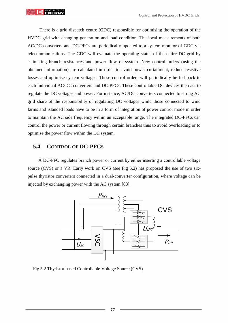
Control and Protection of HVDC Grids
77
There is a grid dispatch centre (GDC) responsible for optimising the operation of the
HVDC grid with changing generation and load condition. The local measurements of both
AC/DC converters and DC-PFCs are periodically updated to a system monitor of GDC via
telecommunications. The GDC will evaluate the operating status of the entire DC grid by
estimating branch resistances and power flow of system. New control orders (using the
obtained information) are calculated in order to avoid power curtailment, reduce resistive
losses and optimise system voltages. These control orders will periodically be fed back to
each individual AC/DC converters and DC-PFCs. These controllable DC devices then act to
regulate the DC voltages and power. For instance, AC/DC converters connected to strong AC
grid share of the responsibility of regulating DC voltages while those connected to wind
farms and islanded loads have to be in a form of integration of power control mode in order
to maintain the AC side frequency within an acceptable range. The integrated DC-PFCs can
control the power or current flowing through certain branches thus to avoid overloading or to
optimise the power flow within the DC system.
5.4 CONTROL OF DC-PFCS
A DC-PFC regulates branch power or current by either inserting a controllable voltage
source (CVS) or a VR. Early work on CVS (see Fig 5.2) has proposed the use of two six-
pulse thyristor converters connected in a dual-converter configuration, where voltage can be
injected by exchanging power with the AC system [88].
CVS
VSC
PINT
UINT
UacPBR
Fig 5.2 Thyristor based Controllable Voltage Source (CVS)

Control and Protection of HVDC Grids
78
CVS
PINT
UINTUac
DC
AC
DC
DC
VSC PBR
Fig 5.3 IGBT based CVS
Alternatively, a CVS can be composed of a combination of an IGBT based AC/DC
converter and a DC/DC converter (see Fig 5.3). Both devices are able to control the power
flow through a certain branch (PBR) by adjusting the injected voltage (UINT). Note that a small
change on the injected voltage (e.g. 5% of system voltage rate) is usually enough to have a
significant effect on power flow since the devices are connected in series with DC branches.
Therefore DC-PFCs will have much smaller rate of voltage and power, compared with the
AC/DC converters that connect AC systems to an HVDC grid. A CVS is thus suitable for
achieving flexible control of power in a cost effective way. However, its disadvantage could
be the disproportionately sized auxiliary transformer, which has to be rated to withstand the
high voltage at system level. An alternative power flow controller [90]-[92] is then proposed
(see Fig 5.4) in order to avoid the use of such an auxiliary transformer.
UINT1
UINT2
VSC
PINT
Fig 5.4 An alternative power flow controller
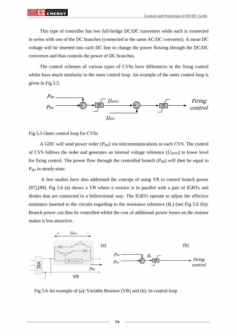
Control and Protection of HVDC Grids
79
This type of controller has two full-bridge DC/DC converters while each is connected
in series with one of the DC branches (connected to the same AC/DC converter). A mean DC
voltage will be inserted into each DC line to change the power flowing through the DC/DC
converters and thus controls the power of DC branches.
The control schemes of various types of CVSs have differences in the firing control
whilst have much similarity in the outer control loop. An example of the outer control loop is
given in Fig 5.5.
PBR
UINTO
PBOPI
UINT
Firing controlPI
Fig 5.5 Outer control loop for CVSs
A GDC will send power order (PBO) via telecommunications to each CVS. The control
of CVS follows the order and generates an internal voltage reference (UINTO) to lower level
for firing control. The power flow through the controlled branch (PBR) will then be equal to
PBO in steady-state.
A few studies have also addressed the concept of using VR to control branch power
[87],[89]. Fig 5.6 (a) shows a VR where a resistor is in parallel with a pair of IGBTs and
diodes that are connected in a bidirectional way. The IGBTs operate to adjust the effective
resistance inserted to the circuits regarding to the resistance reference (Ro) (see Fig 5.6 (b)).
Branch power can thus be controlled whilst the cost of additional power losses on the resistor
makes it less attractive.
UINT
Resistor
VR
(a)
PBR
VSC
PBR
PBOFiring
controlPI
(b)
Ro
Fig 5.6 An example of (a): Variable Resistor (VR) and (b): its control loop

Control and Protection of HVDC Grids
80
5.5 DC VOLTAGE VERSUS POWER DROOP FOR CONVERTERS
Alternative to those DC voltage versus current droop characteristics used for the ACC,
an AC/DC converter can also be implemented with a DC voltage versus power droop as
shown in Fig 5.7 (a). This droop allows the MMC to regulate its own DC voltage by
adjusting the converter power. The DC voltage versus power droop is mathematically given
by:
)()( CMCOCMCO PPUUk (5.1)
where 𝑈𝐶𝑂 and 𝑃𝐶𝑂 are the control orders of voltage and power; 𝑈𝐶𝑀 and 𝑃𝐶𝑀 are the
measurements of converter DC voltage and power. The DC voltage/power droop 𝑘 reflects
the sensitivity of power deviation to DC voltage change.
SM1
SM2
SMn
SM1
SM2
SMn
SM1
SM2
SMn
SM1
SM2
SMn
SM1
SM2
SMn
SM1
SM2
SMn
DC-PFC
PCM
UCO
PCOUCM
k Decoupling Current control
PI
(a)
(b)
+Pdc-Pdc
Vdc
PCO
UCO
UCM
PCM
OPCM
OPCO
UCM
PCM
Fig 5.7 Converter with V/P droop: (a) control structure (b) V/P droop characteristics
In steady state, the actual operation point (OPCO) is located at the droop line (see Fig
5.7) and OPCM is the desirable operating point (OPCM). A change of control orders (e.g. Uco
and Pco) will lead the desirable operating point to move and thus have an impact on both the
actual converter power and system DC power flow.

Control and Protection of HVDC Grids
81
Moreover, if DC-PFCs are integrated, the DC-PFCs act to control the power flow some
DC branches. This will also have an impact on the power flow of the rest system and the
converter power. The actual operating point of a converter could drift away from the
desirable operation point. The GDC will thus have to re-dispatch control orders to optimise
the converter operating. The coordination of converter control and DC-PFC control on power
flow should then be investigated. The impact of re-dispatching control orders on system
operation (e.g. power flow, voltage) should be studied in detail.
5.6 IMPACT OF CHANGING CONTROL ORDERS ON DC POWER
FLOW
The DC power flow expression for a DC grid without any DC-PFC is similar to the
matrix formulation of AC power flow, which is given as:
CMCMCM GUUP (5.2)
where ⨂ is the entry-wise matrix multiplication operator; G is the conductance matrix; PCM
and UCM are vectors representing the converter power and DC voltage:
,1 , ,[ ]T
CM CM i CM mP P PCM
P ,1 , ,[ ]T
CM CM i CM mU U UCM
U (5.3)
Notice that a DC transmission system reactance can be neglected and thus represented
by conductance matrix 𝑮 in Eq. (5.2). Moreover, there may be DC nodes which are not
connected to any converter. These DC nodes can mathematically be considered as connected
to converters but have no power exchange with the AC system (i.e. PCM=0).
Modification of Eq. (5.3) will be needed if DC-PFCs are integrated. Fig 5.8 (a) shows a
HVDC grid composed of m converters and n DC-PFCs.
A small voltage (UINT,j) is created by DC-PFCj to control the power through the local
branch (PBR,2j) to a certain value:
𝑃𝐵𝑅,2𝑗 = 𝑈𝐶𝑀,𝑗 × (𝑈𝐶𝑀,𝑗 − 𝑈𝐶𝑀,2) × 𝐺2𝑗 (5.4)
where 𝑈𝐶𝑀,2 is the converter voltage for VSC2. The installation of a DC-PFC creates a new
node (e.g. node j) which provides an additional dimension for controlling power flow. The
voltage of node j is denoted as 𝑈𝐶𝑀,𝑗. The 𝐺2𝑗 is the conductance between node 2 and node j.
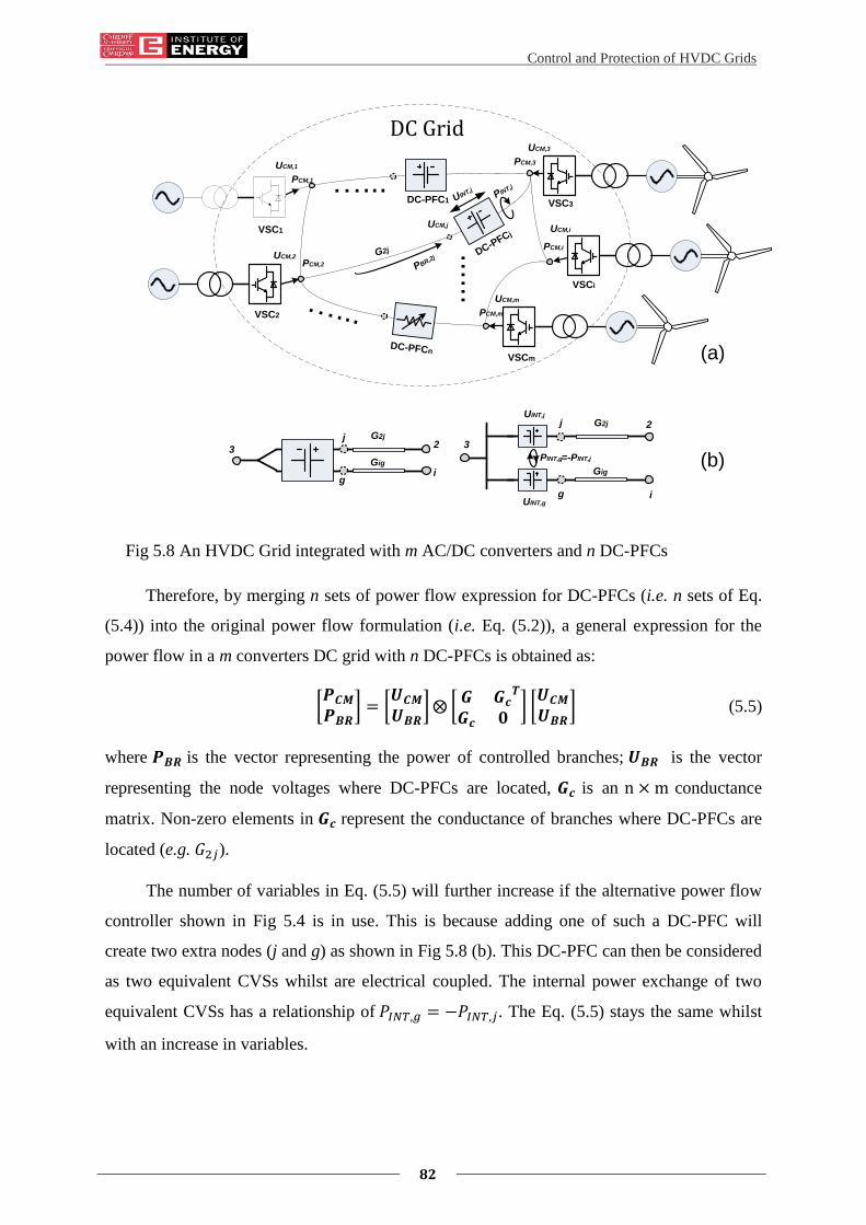
Control and Protection of HVDC Grids
82
......
…...
…...
DC Grid
VSC1
VSC2
VSC3
VSCi
VSCm
DC-PFC1
DC-PFCn
DC-PFCj
UCM,1
G2j
PCM,1
UCM,2
PCM,2
UCM,3
PCM,3
UCM,i
PCM,i
UCM,m
PCM,m
UCM,j
UINT,j
PINT,j
(a)
(b)
G2j
Gig
G2j
Gig
UINT,j
UINT,g
32
i
j3
j
g
g
=-PINT,jPINT,g
2
i
PBR,2j
Fig 5.8 An HVDC Grid integrated with m AC/DC converters and n DC-PFCs
Therefore, by merging n sets of power flow expression for DC-PFCs (i.e. n sets of Eq.
(5.4)) into the original power flow formulation (i.e. Eq. (5.2)), a general expression for the
power flow in a m converters DC grid with n DC-PFCs is obtained as:
[𝑷𝑪𝑴𝑷𝑩𝑹
] = [𝑼𝑪𝑴𝑼𝑩𝑹
]⨂ [𝑮 𝑮𝒄
𝑻
𝑮𝒄 𝟎 ] [𝑼𝑪𝑴𝑼𝑩𝑹
] (5.5)
where 𝑷𝑩𝑹 is the vector representing the power of controlled branches; 𝑼𝑩𝑹 is the vector
representing the node voltages where DC-PFCs are located, 𝑮𝒄 is an n × m conductance
matrix. Non-zero elements in 𝑮𝒄 represent the conductance of branches where DC-PFCs are
located (e.g. 𝐺2𝑗).
The number of variables in Eq. (5.5) will further increase if the alternative power flow
controller shown in Fig 5.4 is in use. This is because adding one of such a DC-PFC will
create two extra nodes (j and g) as shown in Fig 5.8 (b). This DC-PFC can then be considered
as two equivalent CVSs whilst are electrical coupled. The internal power exchange of two
equivalent CVSs has a relationship of 𝑃𝐼𝑁𝑇,𝑔 = −𝑃𝐼𝑁𝑇,𝑗. The Eq. (5.5) stays the same whilst
with an increase in variables.

Control and Protection of HVDC Grids
83
Equation (5.5) mathematically shows the relationship amongst converter voltages,
converter power and the power of controlled branches. The relationship of control orders and
DC power flow is not reflected. Therefore, the next step is to investigate the impact of
changing control orders on system DC power flow.
As previously mentioned the control orders given by the GDC includes both the orders
for MMCs (𝑈𝐶𝑂 , 𝑃𝐶𝑂 and 𝑘) and those for DC-PFCs (𝑃𝐵𝑂). In steady-state, the operating
points of MMCs will follow the droop characteristics (see Eq. (5.1)) and the controlled
branch power will equal to the ordered power for DC-PFCs (i.e. 𝑃𝐵𝑅 = 𝑃𝐵𝑂). Therefore, the
relationship amongst a set of power flow and control orders is given in a matrix form:
𝑷𝑪𝑴 = 𝑷𝑪𝑶 − diag(𝒌) × (𝑼𝑪𝑶 − 𝑼𝑪𝑴)𝑷𝑩𝑹 = 𝑷𝑩𝑶
(5.6)
where, diag(𝒌) is a diagonal matrix representing the droops.
Equation (5.6) can then be re-written into small-signal form:
∆𝑷𝑪𝑴 = ∆𝑷𝑪𝑶 − diag(𝒌) × (∆𝑼𝑪𝑶 − ∆𝑼𝑪𝑴) ∆𝑷𝑩𝑹 = ∆𝑷𝑩𝑶
(5.7)
The small-signal matrix for Eq. (5.5) can also be obtained by differentiation:
[∆𝑷𝑪𝑴∆𝑷𝑩𝑹
] = [𝑱𝒎/𝒎 𝑱𝒎/𝒏𝑱𝒏/𝒎 𝑱𝒏/𝒏
] [∆𝑼𝑪𝑴∆𝑼𝑩𝑹
] (5.8)
where 𝑱𝒎/𝒎 , 𝑱𝒎/𝒏 , 𝑱𝒏/𝒎and 𝑱𝒏/𝒏 form the Jacobian matrix reflecting the power deviation
respecting to the voltage change of converters and DC-PFCs. By combining Eq. (5.7) and Eq.
(5.8) gives:
[∆𝑷𝑪𝑴∆𝑷𝑩𝑹
] = [
𝝏𝑷𝑪𝑴
𝝏𝑷𝑪𝑶
𝝏𝑷𝑪𝑴
𝝏𝑷𝑩𝑶𝝏𝑷𝑩𝑹
𝝏𝑷𝑪𝑶
𝝏𝑷𝑩𝑹
𝝏𝑷𝑩𝑶
] [∆𝑷𝑪𝑶∆𝑷𝑩𝑶
] + [
𝝏𝑷𝑪𝑴
𝝏𝑼𝑪𝑶𝟎
𝝏𝑷𝑩𝑹
𝝏𝑼𝑪𝑶𝟎] [∆𝑼𝑪𝑶𝟎
]
[
𝝏𝑷𝑪𝑴
𝝏𝑷𝑪𝑶
𝝏𝑷𝑪𝑴
𝝏𝑷𝑩𝑶𝝏𝑷𝑩𝑹
𝝏𝑷𝑪𝑶
𝝏𝑷𝑩𝑹
𝝏𝑷𝑩𝑶
] = 𝟏 − [diag(𝒌) 𝟎𝟎 𝟎
] × [𝑱𝒎/𝒎 𝑱𝒎/𝒏𝑱𝒏/𝒎 𝑱𝒏/𝒏
]−𝟏
−𝟏
[
𝝏𝑷𝑪𝑴
𝝏𝑼𝑪𝑶𝟎
𝝏𝑷𝑩𝑹
𝝏𝑼𝑪𝑶𝟎] = 𝟏 − [
diag(𝒌) 𝟎𝟎 𝟎
] × [𝑱𝒎/𝒎 𝑱𝒎/𝒏𝑱𝒏/𝒎 𝑱𝒏/𝒏
]−𝟏
−𝟏
∙ [diag(𝒌) 𝟎𝟎 𝟎
]
(5.9)
Equation (5.9) shows the impact of changing control orders on the converter power and
the power of controlled branch. It can be found that the change of control orders of converters

Control and Protection of HVDC Grids
84
will not affect the power flow of controlled branch while the change of control orders of DC-
PFCs will have an impact on converter power.
Similarly, the impact of changing control orders on system DC voltages can also be
derived as Eq. (5.10):
[∆𝑼𝑪𝑴∆𝑼𝑩𝑹
] = [
𝝏𝑼𝑪𝑴
𝝏𝑷𝑪𝑶
𝝏𝑼𝑪𝑴
𝝏𝑷𝑩𝑶𝝏𝑼𝑩𝑹
𝝏𝑷𝑪𝑶
𝝏𝑼𝑩𝑹
𝝏𝑷𝑩𝑶
] [∆𝑷𝑪𝑶∆𝑷𝑩𝑶
] + [
𝝏𝑼𝑪𝑴
𝝏𝑼𝑪𝑶𝟎
𝝏𝑼𝑩𝑹
𝝏𝑼𝑪𝑶𝟎] [∆𝑼𝑪𝑶𝟎
]
[
𝝏𝑼𝑪𝑴
𝝏𝑷𝑪𝑶
𝝏𝑼𝑪𝑴
𝝏𝑷𝑩𝑶𝝏𝑼𝑩𝑹
𝝏𝑷𝑪𝑶
𝝏𝑼𝑩𝑹
𝝏𝑷𝑩𝑶
] = [𝑱𝒎/𝒎 𝑱𝒎/𝒏𝑱𝒏/𝒎 𝑱𝒏/𝒏
] − [diag(𝒌) 𝟎𝟎 𝟎
]
−𝟏
[
𝝏𝑷𝑪𝑴
𝝏𝑼𝑪𝑶𝟎
𝝏𝑷𝑩𝑹
𝝏𝑼𝑪𝑶𝟎] = [
diag(𝒌) 𝟎𝟎 𝟎
] − [𝑱𝒎/𝒎 𝑱𝒎/𝒏𝑱𝒏/𝒎 𝑱𝒏/𝒏
]−𝟏
∙ [diag(𝒌) 𝟎𝟎 𝟎
]
(5.10)
Equation (5. 10) illustrates that the change of control orders of both converters and DC-
PFCs will have an impact on DC system voltages.
Both Eq. (5.9) and Eq. (5.10) show the linearised relationship of the control orders and
system power and voltage. The impact of changing control orders on system operation can
then be evaluated. Moreover, the linearised relationship can also be used for GDC to re-
dispatch the control orders for achieving desirable system power flow. For example, the GDC
would like to change the power flow through converters by ∆𝑷𝑪𝑴 while have a change of
∆𝑼𝑪𝑴 in DC voltages. By solving the inverse function of Eq. (5.9) and Eq. (5.10), the
required amount of change in control orders can be estimated.
5.7 OPTIMISATION OF DC POWER FLOW
A. Objective Function
This study specifically addresses the optimisation of wind power delivery as it is very
likely that a DC grid will be integrated with remote offshore wind farms. It is then reasonable
to have an objective function of maximising the wind power delivery to the onshore system,
which aims to:
Reduce the curtailment of wind power due to overload of DC branch.
Reduce the resistive line losses.
This can be expressed by:

Control and Protection of HVDC Grids
85
𝑀𝑎𝑥 ∑ 𝑃𝑖𝑛𝑣,𝑖𝑟1 = 𝑀𝑎𝑥∑ (𝑃𝑤𝑓,𝑓 − 𝑃𝑐𝑢𝑟,𝑓)
𝑔1 − ∑ 𝑃𝑙𝑜𝑠𝑠
𝑣1 − ∑ 𝑃𝐼𝑁𝑇_𝑉𝑅
𝑦1 (5.11)
where ∑ 𝑃𝑖𝑛𝑣,𝑖𝑟
1 represents the total power received by onshore inverters which equals to the
total available wind power subtracted by the power curtailment ∑ (𝑃𝑤𝑓,𝑓 − 𝑃𝑐𝑢𝑟,𝑓)𝑔1 , total line
losses ∑ 𝑃𝑙𝑜𝑠𝑠𝑣1 and the power loss of the inserted resistance of VRs ∑ 𝑃𝐼𝑁𝑇_𝑉𝑅
𝑦
1 (if only VRs
are in use).
B. Constraints
The operation of a HVDC grid is subjected to both equality constraints and inequality
constraints. These constraints are listed below i.e. Eq. (5.12) – Eq. (5.14):
Power flow equality constraints:
The power is balanced amongst a converter at a node and its connected DC branches
while the power of a controlled branch should equal to the control order given by a DC-PFC:
𝑃𝐶𝑀,𝑖 − 𝑃𝑇,𝑖 = 0
𝑃𝐵𝑂,𝑗 − 𝑃𝐵𝑅,𝑗 = 0 (5.12)
where 𝑃𝑇,𝑖 is the total power transmitted through the DC branches to converters.
DC system inequality constraints:
DC system inequality constraints include the physical power constraints of converters,
voltage constraints of converters and power constraints of DC branches:
𝑃𝐶𝑀,𝑖𝑚𝑖𝑛 ≤ 𝑃𝐶𝑀,𝑖 ≤ 𝑃𝐶𝑀,𝑖
𝑚𝑎𝑥
𝑈𝐶𝑀,𝑖𝑚𝑖𝑛 ≤ 𝑈𝐶𝑀,𝑖 ≤ 𝑈𝐶𝑀,𝑖
𝑚𝑎𝑥
𝑃𝐵𝑅,𝑖𝑚𝑖𝑛 ≤ 𝑃𝐵𝑅,𝑖 ≤ 𝑃𝐵𝑅,𝑖
𝑚𝑎𝑥
(5.13)
The minimum physical power constraint 𝑃𝐶𝑀,𝑖𝑚𝑖𝑛 is the negative form of 𝑃𝐶𝑀,𝑖
𝑚𝑎𝑥 ,
indicating the constraint for bidirectional power flow.
Control inequality constraints:
The boundaries of control orders setting are given as:
𝑃𝐶𝑂,𝑖𝑚𝑖𝑛 ≤ 𝑃𝐶𝑂,𝑖 ≤ 𝑃𝐶𝑂,𝑖
𝑚𝑎𝑥
𝑈𝐶𝑂,𝑖𝑚𝑖𝑛 ≤ 𝑈𝐶𝑂,𝑖 ≤ 𝑈𝐶𝑂,𝑖
𝑚𝑎𝑥
𝑃𝐵𝑂,𝑖𝑚𝑖𝑛 ≤ 𝑃𝐵𝑂,𝑖 ≤ 𝑃𝐵𝑂,𝑖
𝑚𝑎𝑥
(5.14)
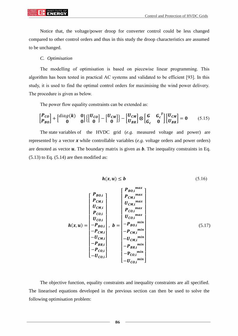
Control and Protection of HVDC Grids
86
Notice that, the voltage/power droop for converter control could be less changed
compared to other control orders and thus in this study the droop characteristics are assumed
to be unchanged.
C. Optimisation
The modelling of optimisation is based on piecewise linear programming. This
algorithm has been tested in practical AC systems and validated to be efficient [93]. In this
study, it is used to find the optimal control orders for maximising the wind power delivery.
The procedure is given as below.
The power flow equality constraints can be extended as:
[𝑷𝑪𝑶𝑷𝑩𝑶
] + [𝑑𝑖𝑎𝑔(𝒌) 𝟎
𝟎 𝟎] [𝑼𝑪𝑶𝟎] − [
𝑼𝑪𝑴𝟎] − [
𝑼𝑪𝑴𝑼𝑩𝑹
]⨂ [𝑮 𝑮𝒄
𝑻
𝑮𝒄 𝟎 ] [𝑼𝑪𝑴𝑼𝑩𝑹
] = 𝟎 (5.15)
The state variables of the HVDC grid (e.g. measured voltage and power) are
represented by a vector 𝒙 while controllable variables (e.g. voltage orders and power orders)
are denoted as vector 𝒖. The boundary matrix is given as b. The inequality constraints in Eq.
(5.13) to Eq. (5.14) are then modified as:
𝒉(𝒙, 𝒖) ≤ 𝒃 (5.16)
𝒉(𝒙, 𝒖) =
[ 𝑷𝑩𝑶,𝒊𝑷𝑪𝑴,𝒊𝑼𝑪𝑴,𝒊𝑷𝑪𝑶,𝒊𝑼𝑪𝑶,𝒊−𝑷𝑩𝑶,𝒊−𝑷𝑪𝑴,𝒊−𝑼𝑪𝑴,𝒊−𝑷𝑩𝑹,𝒊−𝑷𝑪𝑶,𝒊−𝑼𝑪𝑶,𝒊]
, 𝒃 =
[ 𝑷𝑩𝑶,𝒊
𝒎𝒂𝒙
𝑷𝑪𝑴,𝒊𝒎𝒂𝒙
𝑼𝑪𝑴,𝒊𝒎𝒂𝒙
𝑷𝑪𝑶,𝒊𝒎𝒂𝒙
𝑼𝑪𝑶,𝒊𝒎𝒂𝒙
−𝑷𝑩𝑶,𝒊𝒎𝒊𝒏
−𝑷𝑪𝑴,𝒊𝒎𝒊𝒏
−𝑼𝑪𝑴,𝒊𝒎𝒊𝒏
−𝑷𝑩𝑹,𝒊𝒎𝒊𝒏
−𝐏𝑪𝑶,𝒊𝒎𝒊𝒏
−𝑼𝑪𝑶,𝒊𝒎𝒊𝒏
]
(5.17)
The objective function, equality constraints and inequality constraints are all specified.
The linearised equations developed in the previous section can then be used to solve the
following optimisation problem:

Control and Protection of HVDC Grids
87
Max ∑𝑃𝑖𝑛𝑣,𝑖
𝑟
1
s. t. [𝑷𝑪𝑶𝑷𝑩𝑶
] + [diag(𝒌) 𝟎𝟎 𝟎
] [𝑼𝑪𝑶𝟎] − [
𝑼𝑪𝑴𝟎] − [
𝑼𝑪𝑴𝑼𝑩𝑹
]⨂ [𝑮 𝑮𝒄
𝑻
𝑮𝒄 𝟎 ] [𝑼𝑪𝑴𝑼𝑩𝑹
] = 𝟎
𝒉(𝒙, 𝒖) ≤ 𝒃
(5.18)
The maximisation of wind power delivery can be achieved by re-dispatching optimised
control orders of converters and DC-PFCs. A flow chart of optimisation is presented in Fig
5.9. The optimisation starts with the specification of DC system topology (e.g. numbers of
DC devices, connections). This is followed by the initialisation of control orders and system
conductance. After the initialisation, the expression of power flow needs to be linearised
before solving the equality constraints. The solution to the equality constraints then takes a
few iterations until the error between 𝑷𝑪𝑴 , 𝑷𝑩𝑶 and 𝑷𝑻 , 𝑷𝑩𝑹 is smaller than a defined value
(i.e. ζ). Notice that well-designed initialisation can reduce the number of iterations. The
outputs are the updated vectors 𝒉(𝒙, 𝒖) and linearised matrix 𝝏𝒉(𝒙,𝒖)
𝝏𝒖. The required amount of
change in the vector of control orders (i.e. ∆𝒖(𝑖+1) ) can then be estimated using linear
programming. An additional step is included to re-assess all the constraints with the updated
control orders. If the error between the previous results and the new iteration is less than a
defined value (i.e. ∆𝒖(𝑖+1) − ∆𝒖(𝑖) < µ), a precise vector of control orders will eventually be
obtained and output for the maximisation of wind power delivery.
Specify numbers of converters and DC-PFCs;Specify system topology
Initialise control orders, system conductance
Linearise the expression of controlling power
flow
Solve Power Flow Equality Constraints
(PCM-PT)<ζ ?
Yes
No
Obtain newh(x,u); ∂h(x,u)/∂u
Solve all Inquality Constraints
Yes
No
Optimisation achieved
∆u - ∆u <µ?(i+1) (i)
Obatin new control orders:
u(i+1)
Obtain and Update:u =∆u +u
(i+1) (i)(i+1)
Fig 5.9 Flow chart of solving optimal DC power flow
Control and Protection of HVDC Grids
88
5.8 CASE STUDY
The effectiveness of coordinating control of DC devices on optimising the wind power
is validated on a 9-terminal DC system integrated with one CVS (see Fig 5.10). This system
has a DC voltage rate of +/-400 kV. The delivery of wind power is through four offshore
converters which can equivalently be considered as in power control mode in this study.
However, the equivalences of “power orders” are naturally determined by the offshore wind
conditions. The relationship between the “power orders” and wind conditions is presented in
detail in [94].These offshore converters will import all the generated wind power to the DC
system if the power does not reach the physical rate of any DC branch or converter.
Conversely, in the events of overloading, the wind farms will have to reduce the generation
which leads to the curtailment of wind power.
At the receiving end, there are four onshore rectifiers with DC voltage droop control.
Converters VSC1 to VSC4 are connected to strong AC system thus share the responsibility of
regulating DC voltage. Another converter VSC6 is assumed to be connected with a weak AC
system and thus consistently in power control mode.
A CVS is located at node N2 to avoid overloading of a DC branch (i.e. initially controls
the power of Link N2-N7) and coordinate with converters on optimising the power delivery.
The initial control setting and physical rate of controllable DC devices are given in
Table I. The sign convention of power in this study is defined as:
Import power to the DC Grid: Positive (+)
Export power from the DC Grid: Negative (-)

Control and Protection of HVDC Grids
89
N1
N2
N3
N4 N5
N7 N6
N8
VSC1
VSC2
VSC3
VSC4 VSC5
VSC6 VSC7
VSC8
VSC9
WF1
WF2
WF3
WF4
GS1
GS2
GS3
GS4
GS5
DC-PFC
Cable
Overhead Line
200km
200km
200km
300km
400km
500km
200km
200km
200km
200km
200km
(0.0144Ω/km,Max. current:3000A)
(0.0095Ω/km,Max. current:1962A)
N9
Fig 5.10 A 9-terminal DC system with the integration of a DC-PFC
Table 5-1 PARAMETERS OF DC DEVICES
DC device Rate of device Control Mode Control Setting
VSC1 +/-420kV; 2400MW Voltage droop control PCO=1500MW ; VCO=818.17kV; k=-60 MW/kV;
VSC2 +/-420kV; 2400MW Voltage droop control PCO=-1900MW ; VCO=809.54kV; k=-100MW/kV;
VSC3 +/-420kV; 2400MW DC Voltage control VCO=800kV;
VSC4 +/-420kV; 1200MW Voltage droop control PCO=-800MW ; VCO=802.17kV; k=-60 MW/kV;
VSC5 +/-420kV; 2400MW power control PCO=500MW; (Case one)
PCO=400MW; (Case Two/Three)
VSC6 +/-420kV; 200MW “power control” PCO=-100MW; (Case Two/Three)
VSC7 +/-420kV; 2400MW “power control” PCO=1000MW; (Case one)
PCO=500MW; (Case Two/Three)
VSC8 +/-420kV; 1500MW “power control” PCO=500MW; (Case One)
PCO=200MW; (Case Two/Three)
VSC9 +/-420kV; 1500MW “power control” PCO=500MW; (Case One)
PCO=200MW; (Case Two/Three)
DC-PFC +/-15kV Branch power control PBO=-463.4MW(inserted zero voltage);
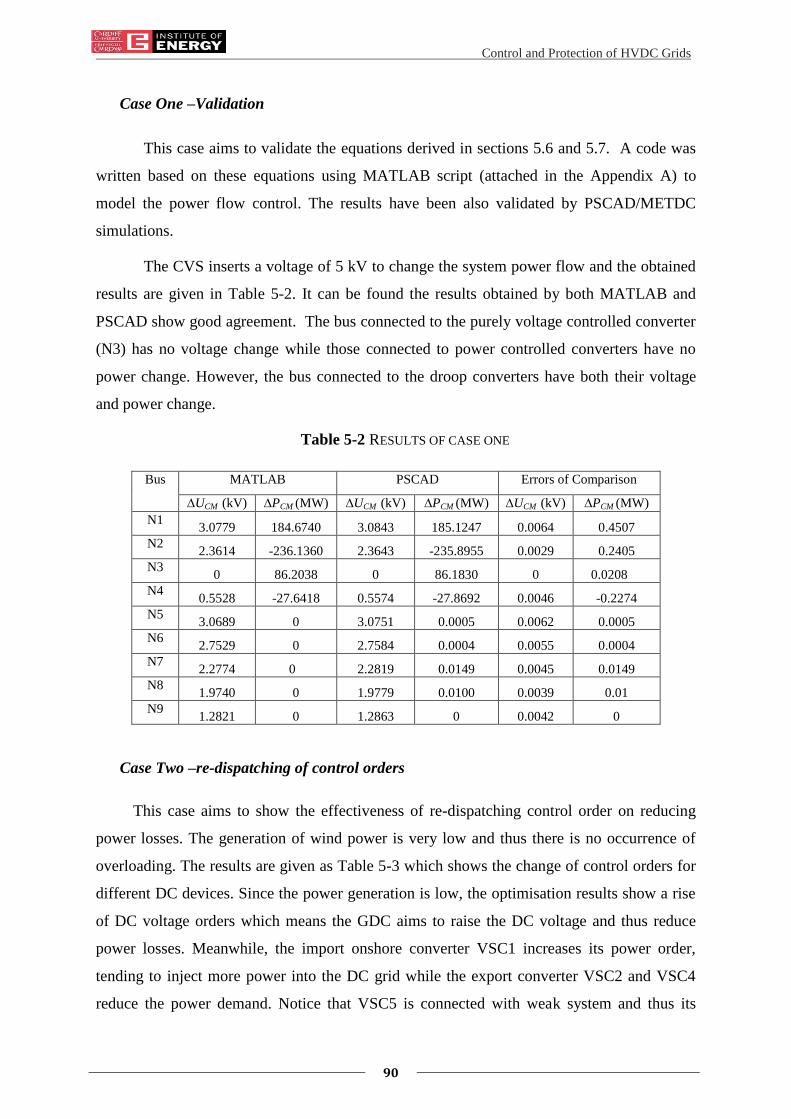
Control and Protection of HVDC Grids
90
Case One –Validation
This case aims to validate the equations derived in sections 5.6 and 5.7. A code was
written based on these equations using MATLAB script (attached in the Appendix A) to
model the power flow control. The results have been also validated by PSCAD/METDC
simulations.
The CVS inserts a voltage of 5 kV to change the system power flow and the obtained
results are given in Table 5-2. It can be found the results obtained by both MATLAB and
PSCAD show good agreement. The bus connected to the purely voltage controlled converter
(N3) has no voltage change while those connected to power controlled converters have no
power change. However, the bus connected to the droop converters have both their voltage
and power change.
Table 5-2 RESULTS OF CASE ONE
Bus MATLAB PSCAD Errors of Comparison
∆UCM (kV) ∆PCM (MW) ∆UCM (kV) ∆PCM (MW) ∆UCM (kV) ∆PCM (MW)
N1 3.0779 184.6740 3.0843 185.1247 0.0064 0.4507
N2 2.3614 -236.1360 2.3643 -235.8955 0.0029 0.2405
N3 0 86.2038 0 86.1830 0 0.0208
N4 0.5528 -27.6418 0.5574 -27.8692 0.0046 -0.2274
N5 3.0689 0 3.0751 0.0005 0.0062 0.0005
N6 2.7529 0 2.7584 0.0004 0.0055 0.0004
N7 2.2774 0 2.2819 0.0149 0.0045 0.0149
N8 1.9740 0 1.9779 0.0100 0.0039 0.01
N9 1.2821 0 1.2863 0 0.0042 0
Case Two –re-dispatching of control orders
This case aims to show the effectiveness of re-dispatching control order on reducing
power losses. The generation of wind power is very low and thus there is no occurrence of
overloading. The results are given as Table 5-3 which shows the change of control orders for
different DC devices. Since the power generation is low, the optimisation results show a rise
of DC voltage orders which means the GDC aims to raise the DC voltage and thus reduce
power losses. Meanwhile, the import onshore converter VSC1 increases its power order,
tending to inject more power into the DC grid while the export converter VSC2 and VSC4
reduce the power demand. Notice that VSC5 is connected with weak system and thus its
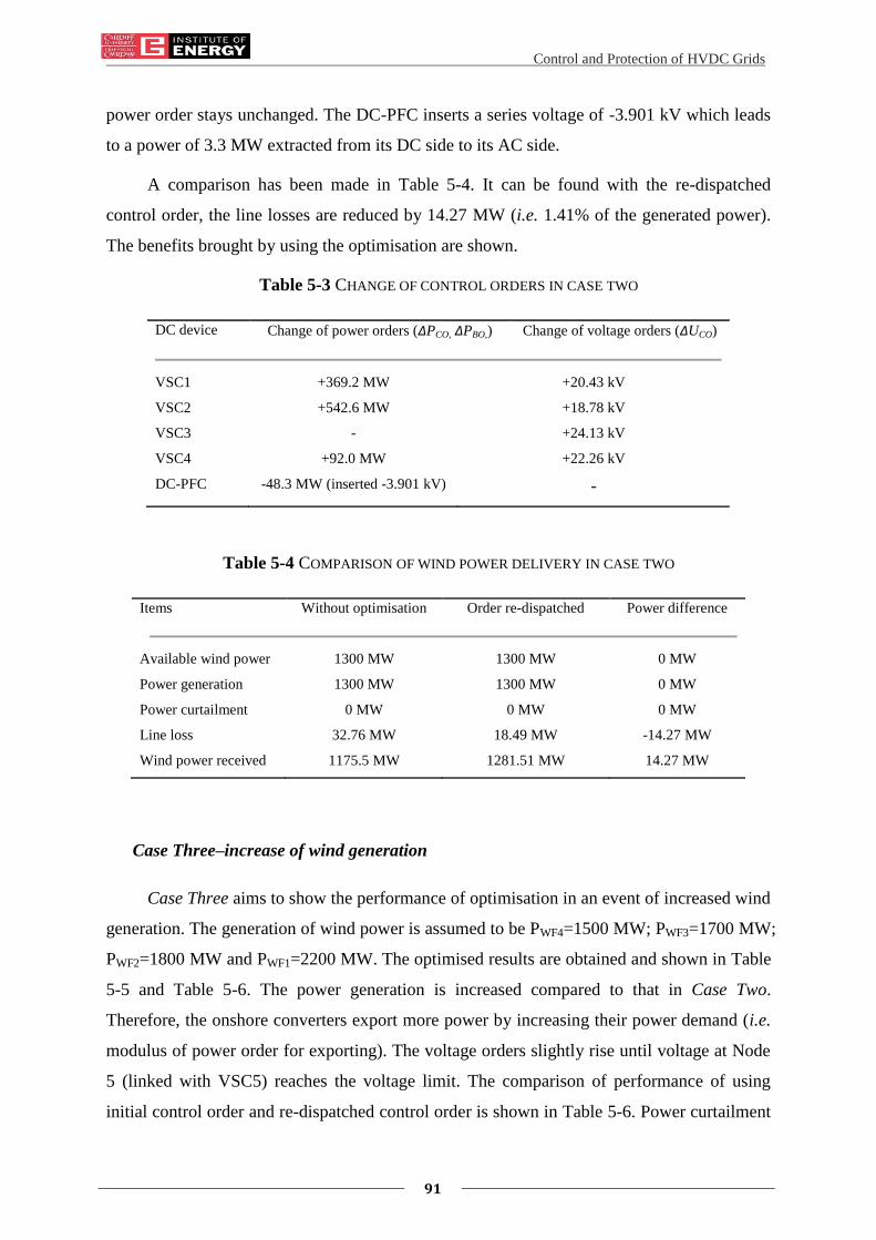
Control and Protection of HVDC Grids
91
power order stays unchanged. The DC-PFC inserts a series voltage of -3.901 kV which leads
to a power of 3.3 MW extracted from its DC side to its AC side.
A comparison has been made in Table 5-4. It can be found with the re-dispatched
control order, the line losses are reduced by 14.27 MW (i.e. 1.41% of the generated power).
The benefits brought by using the optimisation are shown.
Table 5-3 CHANGE OF CONTROL ORDERS IN CASE TWO
DC device Change of power orders (∆PCO, ∆PBO,) Change of voltage orders (∆UCO)
VSC1 +369.2 MW +20.43 kV
VSC2 +542.6 MW +18.78 kV
VSC3 - +24.13 kV
VSC4 +92.0 MW +22.26 kV
DC-PFC -48.3 MW (inserted -3.901 kV) -
Table 5-4 COMPARISON OF WIND POWER DELIVERY IN CASE TWO
Items Without optimisation Order re-dispatched Power difference
Available wind power 1300 MW 1300 MW 0 MW
Power generation 1300 MW 1300 MW 0 MW
Power curtailment 0 MW 0 MW 0 MW
Line loss 32.76 MW 18.49 MW -14.27 MW
Wind power received 1175.5 MW 1281.51 MW 14.27 MW
Case Three–increase of wind generation
Case Three aims to show the performance of optimisation in an event of increased wind
generation. The generation of wind power is assumed to be PWF4=1500 MW; PWF3=1700 MW;
PWF2=1800 MW and PWF1=2200 MW. The optimised results are obtained and shown in Table
5-5 and Table 5-6. The power generation is increased compared to that in Case Two.
Therefore, the onshore converters export more power by increasing their power demand (i.e.
modulus of power order for exporting). The voltage orders slightly rise until voltage at Node
5 (linked with VSC5) reaches the voltage limit. The comparison of performance of using
initial control order and re-dispatched control order is shown in Table 5-6. Power curtailment

Control and Protection of HVDC Grids
92
occurs in both events due to the overloading of Link N4-N5 (Algorithm for power
curtailment is introduced in [94]). However, with the re-dispatched control order, the DC-
PFC aims to deliver +77.8 MW more power through Link N2-N7 and the voltage of VSC4
tends to rise to mitigate the overloading. This results in the reduction of power curtailment by
497.7MW. However, as more power is delivered using the re-dispatched orders, the line loss
is increased. The total power received is increased by 487.79 MW.
Table 5-5 CHANGE OF CONTROL ORDERS IN CASE THREE
DC device Change of power orders (∆PCO, ∆PBO,) Change of voltage orders (∆UCO)
VSC1 -665.3 MW +6.621 kV
VSC2 -5.69 MW +5.222 kV
VSC3 - +6.780 kV
VSC4 -400.0MW +7.303 kV
DC-PFC +77.8 MW (inserted +3.525 kV) -
Table 5-6 COMPARISON OF WIND POWER DELIVERY IN CASE THREE
Items Order unchanged Order Re-dispatched Power difference
Available wind power 7200 MW 7200 MW 0 MW
Power generation 4801.7 MW 5299.4 MW 497.7 MW
Power curtailment 2398.3 MW 1900.6 MW -497.7 MW
Line loss 152.26 MW 162.17 MW 9.91 MW
Wind power received 4649.44 MW 5137.23 MW 487.79 MW

Control and Protection of HVDC Grids
93
5.9 SUMMARY
This chapter has proposed a method to coordinate the control of AC/DC converters and
DC-PFCs thus to optimise the power flow within a DC Grid. An analytical expression has
been derived to illustrate the impact of changing control orders on system power flow. The
effectiveness of proposed methods has been demonstrated by two case studies with different
conditions of wind generation. Results have shown that by the re-dispatching of optimised
control orders, both the curtailment of wind power and the line losses are significantly
reduced.

Control and Protection of HVDC Grids
94
Chapter 6
6. HVDC Grid Protection: Open Grid
Method
6.1 INTRODUCTION
The Open Grid [77] method was proposed for DC network protection to increase the
speed of fault current interruption and reduce the duty of individual DC-CB for blocking a
fault. Within this method, each DC-CB trips rapidly based on local measurements (e.g.
overcurrent, undervoltage) without discrimination and then DC-CBs re-close to discriminate
at healthy circuits. This chapter develops the protection algorithms which can meet DC
protection requirement with different fault types, locations and fault impedances. The
analysis of the fault behaviours in the event of a DC fault has also been given. Different DC
fault characteristics have been described. Further validation of the robustness of the Open
Grid via simulation models developed in PSCAD/EMTDC has been provided. Tests have
shown that the Open Grid can successfully detect and discriminate all DC faults in different
fault conditions in a meshed DC grid.
6.2 DC GRID PROTECTION REVIEW
The intention of building HVDC grids raises many research topics. Amongst those, a
critical one is the protection of DC networks. Unlike faults that occur in an AC system where
the propagation of fault current is limited by relatively large system inductance, the fault
current rise and propagation in a DC system is much faster. Moreover, the system inductance
only affects the rate of rise of the DC fault current, but not the current magnitude. Therefore,
the anticipated speed of DC system protection acting to isolate a DC fault should be much
faster than that of AC system protection. Consequently, protection algorithms have to be
developed to detect a DC fault and interrupt the DC fault current within a very short time (e.g.
2-3 ms [97]-[99]). A desirable outcome of this will be a lower fault current interruption
requirement and reduce the energy dissipation requirements in DC-CBs.
There have been several methods of DC network protection proposed in [100]-[114].
Early stage work [100] presents the “handshaking method” within which DC fault currents
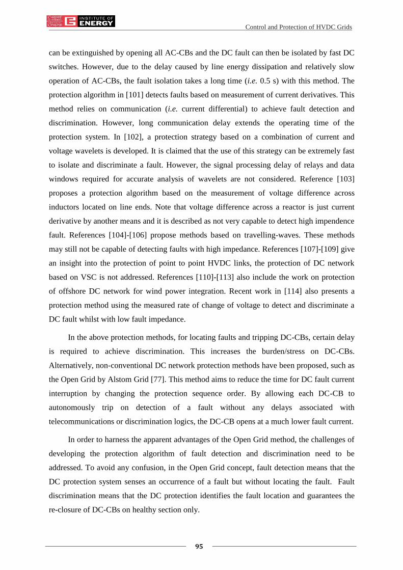
Control and Protection of HVDC Grids
95
can be extinguished by opening all AC-CBs and the DC fault can then be isolated by fast DC
switches. However, due to the delay caused by line energy dissipation and relatively slow
operation of AC-CBs, the fault isolation takes a long time (i.e. 0.5 s) with this method. The
protection algorithm in [101] detects faults based on measurement of current derivatives. This
method relies on communication (i.e. current differential) to achieve fault detection and
discrimination. However, long communication delay extends the operating time of the
protection system. In [102], a protection strategy based on a combination of current and
voltage wavelets is developed. It is claimed that the use of this strategy can be extremely fast
to isolate and discriminate a fault. However, the signal processing delay of relays and data
windows required for accurate analysis of wavelets are not considered. Reference [103]
proposes a protection algorithm based on the measurement of voltage difference across
inductors located on line ends. Note that voltage difference across a reactor is just current
derivative by another means and it is described as not very capable to detect high impendence
fault. References [104]-[106] propose methods based on travelling-waves. These methods
may still not be capable of detecting faults with high impedance. References [107]-[109] give
an insight into the protection of point to point HVDC links, the protection of DC network
based on VSC is not addressed. References [110]-[113] also include the work on protection
of offshore DC network for wind power integration. Recent work in [114] also presents a
protection method using the measured rate of change of voltage to detect and discriminate a
DC fault whilst with low fault impedance.
In the above protection methods, for locating faults and tripping DC-CBs, certain delay
is required to achieve discrimination. This increases the burden/stress on DC-CBs.
Alternatively, non-conventional DC network protection methods have been proposed, such as
the Open Grid by Alstom Grid [77]. This method aims to reduce the time for DC fault current
interruption by changing the protection sequence order. By allowing each DC-CB to
autonomously trip on detection of a fault without any delays associated with
telecommunications or discrimination logics, the DC-CB opens at a much lower fault current.
In order to harness the apparent advantages of the Open Grid method, the challenges of
developing the protection algorithm of fault detection and discrimination need to be
addressed. To avoid any confusion, in the Open Grid concept, fault detection means that the
DC protection system senses an occurrence of a fault but without locating the fault. Fault
discrimination means that the DC protection identifies the fault location and guarantees the
re-closure of DC-CBs on healthy section only.

Control and Protection of HVDC Grids
96
The priority is to design an algorithm quickly detecting a DC fault (e.g. <1 ms). The
challenge is to quickly determine which sections are healthy, so the associated DC-CBs can
be reclosed. This paper addresses these challenges and contributes on the following items:
• To develop the algorithms based on DC voltage and DC current for the detection and
discrimination of both pole to pole faults and pole to ground faults.
• To analyse the voltage and current profiles following the action of protection system.
• To validate and test the Open Grid in different fault events.
6.3 BASIC IDEAS OF OPEN GRID PROTECTION APPROACH
The core idea of the Open Grid is to change the protection sequence thus to block the
fault current before spending time on discriminating or locating a DC fault (see Fig 6.1 (a)).
Multiple DC-CBs (may include some on healthy sections of the grid) simultaneously open to
share fault current interruption duty based only on the local measurements of the breaker (e.g.
overcurrent, undervoltage or even some combinations of current and voltage profiles). The
fault current will then be interrupted with a much shorter time (and thus smaller magnitude)
compared to using conventional method (see Fig 6.1 (b)). Apparently this will bring down the
current breaking requirements of DC protection devices and hence their cost.
The protection system will then locate and discriminate the fault based on the profiles
such as residual DC voltages. The DC-CBs that are not located at the faulted section will re-
close. Notice that the temporary open of more sections will not cause more disturbances to
system since the discrimination will only take several milliseconds without any fault current.
In fact, more sections could potentially get opened which might spare some portions of the
system from the voltage depression, comparing to the use of conventional method which will
take longer time to isolate the fault.
0
detectlocate/
discriminate open
0
detectlocate/
discriminateopen re-close(a)
(b)
Fault current rising
Fault current rising
t (ms)
t (ms)
1 3 6
4
7
1 6
Fig 6.1 Action sequence of: (a) Open Grid protection method; (b) Conventional DC grid
protection method

Control and Protection of HVDC Grids
97
6.4 FAULT DETECTION ALGORITHM
When a DC fault occurs between the poles of a HVDC grid, the DC voltage collapses
and the fault current, fed from the ac system via the converters, increases rapidly (i.e. within a
few milliseconds). As the fault propagating in a DC system is extremely fast, fault detection
systems relying on communication systems will not be able to respond in time to prevent the
fault currents reaching excessively high values. Therefore, the use of local time
measurements of DC voltage (𝑉𝑑𝑐), DC current (𝐼𝑑𝑐), current direction and their derivatives
(𝑑𝑉𝑑𝑐
𝑑𝑡 and
𝑑𝐼𝑑𝑐
𝑑𝑡) at each DC-CB are the preferred signals for detection of DC fault.
An example of using local measurements to detect a DC fault is given in Fig 6.2 where
a solid pole to pole fault is applied at the middle of one branch of a two-VSC, two-branch DC
system. The system is rated at +/-200 kV and both branches are 200 km overhead lines
(OHLs) which share the pre-fault current flowing from Bus B to Bus A. The DC-CBs (i.e. A1,
A2, B1, and B2) are located at both ends of each branch. The DC-CBs are placed in series
with reactors (e.g. 0.1 H) to limit the rate of rise of fault currents.
A1
VSC VSC
Bus A Bus B
B1
A2 B2
RectifierInverter
Fig 6.2 One line diagram of the two-VSC, two-branch DC system
The fault occurs at the middle point of the circuit A1-B1 at 10 ms. Fig 6.3 shows the
voltages, currents and their derivatives which are measured at DC-CBs B1 (faulted) and B2
(healthy). Notice that, in this test, the DC-CBs remain closed and VSCs stay unblocked. It
can be observed that the voltage wave front takes 0.5 ms to reach B1 and another 0.6 ms to
oscillate to below zero. However, the change of voltage at B2 is much smaller than at B1 due
to the presence of the reactors associated with DC-CBs which separate these two
measurement points. Meanwhile, the current at B1 doubles within 1 ms after fault inception
whilst the current direction of B2 tends to reverse to infeed the faulted point.
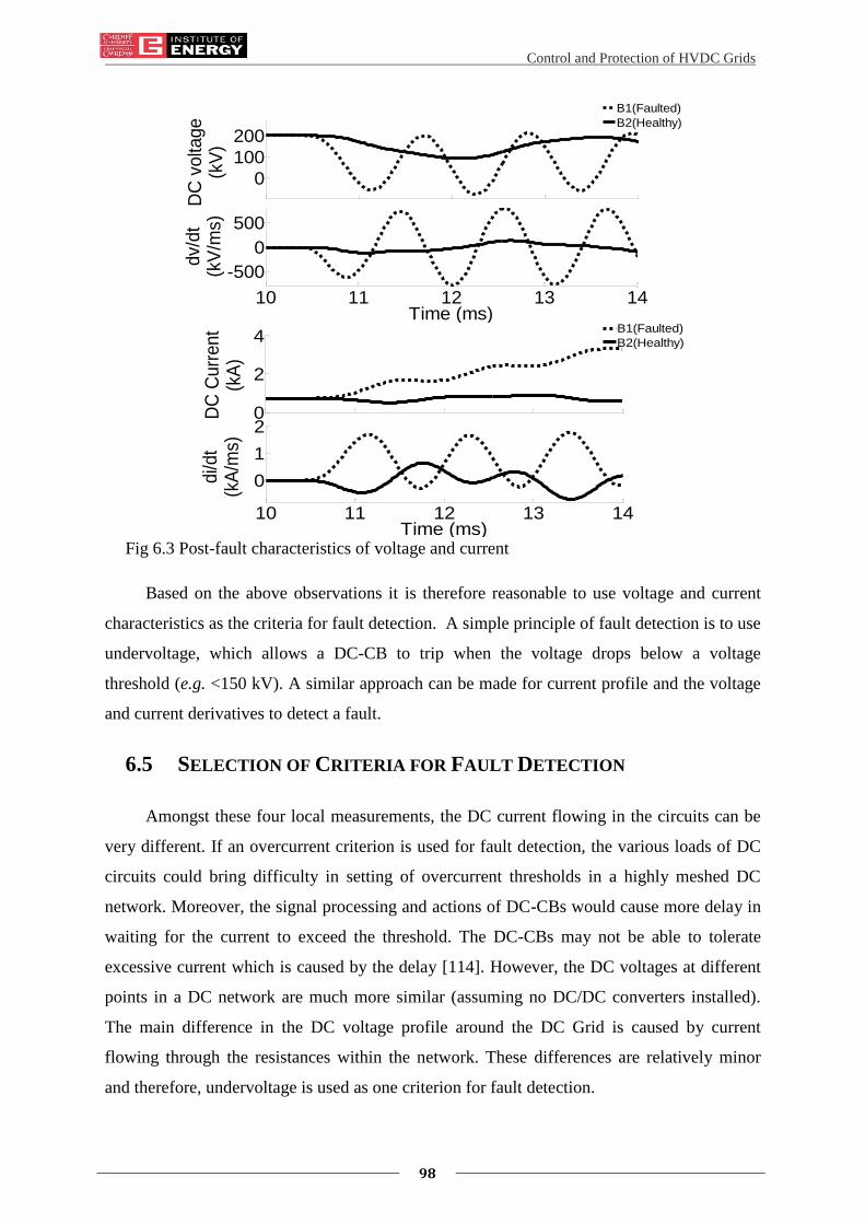
Control and Protection of HVDC Grids
98
Fig 6.3 Post-fault characteristics of voltage and current
Based on the above observations it is therefore reasonable to use voltage and current
characteristics as the criteria for fault detection. A simple principle of fault detection is to use
undervoltage, which allows a DC-CB to trip when the voltage drops below a voltage
threshold (e.g. <150 kV). A similar approach can be made for current profile and the voltage
and current derivatives to detect a fault.
6.5 SELECTION OF CRITERIA FOR FAULT DETECTION
Amongst these four local measurements, the DC current flowing in the circuits can be
very different. If an overcurrent criterion is used for fault detection, the various loads of DC
circuits could bring difficulty in setting of overcurrent thresholds in a highly meshed DC
network. Moreover, the signal processing and actions of DC-CBs would cause more delay in
waiting for the current to exceed the threshold. The DC-CBs may not be able to tolerate
excessive current which is caused by the delay [114]. However, the DC voltages at different
points in a DC network are much more similar (assuming no DC/DC converters installed).
The main difference in the DC voltage profile around the DC Grid is caused by current
flowing through the resistances within the network. These differences are relatively minor
and therefore, undervoltage is used as one criterion for fault detection.
0
100
200
DC
voltage
(kV
)
10 11 12 13 14
-500
0
500
Time (ms)
dv/d
t(k
V/m
s)
B1(Faulted)
B2(Healthy)
0
2
4
DC
Curr
ent
(kA
)
10 11 12 13 14
0
1
2
Time (ms)
di/d
t(k
A/m
s)
B1(Faulted)
B2(Healthy)
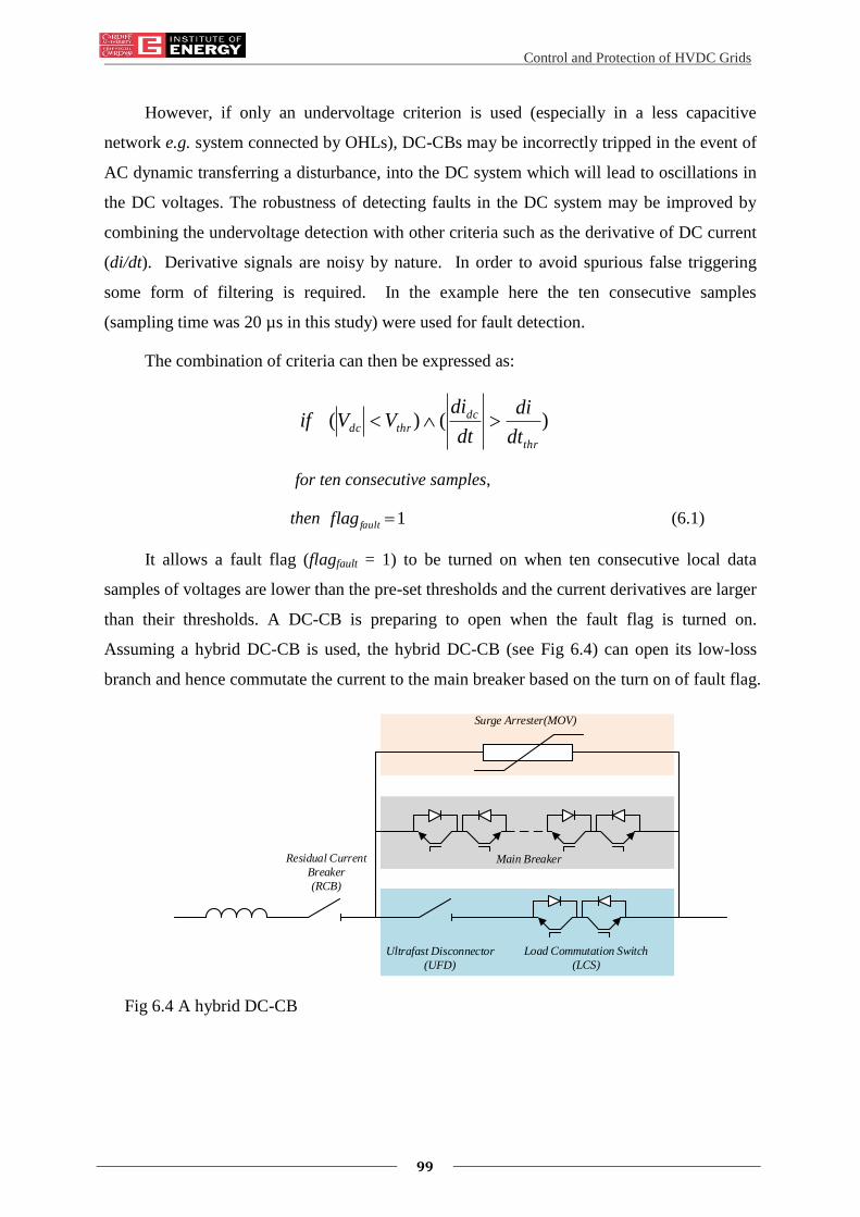
Control and Protection of HVDC Grids
99
However, if only an undervoltage criterion is used (especially in a less capacitive
network e.g. system connected by OHLs), DC-CBs may be incorrectly tripped in the event of
AC dynamic transferring a disturbance, into the DC system which will lead to oscillations in
the DC voltages. The robustness of detecting faults in the DC system may be improved by
combining the undervoltage detection with other criteria such as the derivative of DC current
(di/dt). Derivative signals are noisy by nature. In order to avoid spurious false triggering
some form of filtering is required. In the example here the ten consecutive samples
(sampling time was 20 µs in this study) were used for fault detection.
The combination of criteria can then be expressed as:
)()(thr
dc
thrdcdt
di
dt
diVVif
for ten consecutive samples,
then 1faultflag (6.1)
It allows a fault flag (flagfault = 1) to be turned on when ten consecutive local data
samples of voltages are lower than the pre-set thresholds and the current derivatives are larger
than their thresholds. A DC-CB is preparing to open when the fault flag is turned on.
Assuming a hybrid DC-CB is used, the hybrid DC-CB (see Fig 6.4) can open its low-loss
branch and hence commutate the current to the main breaker based on the turn on of fault flag.
Residual Current
Breaker
(RCB)
Ultrafast Disconnector
(UFD)
Load Commutation Switch
(LCS)
Main Breaker
Surge Arrester(MOV)
Fig 6.4 A hybrid DC-CB

Control and Protection of HVDC Grids
100
6.6 DISCRIMINATION BY INTEGRATION OF CURRENT IN TRANSIENTS
The first step of the discrimination is to determine whether the main breaker should
open or the low loss branch should re-close. The decision can be made based on integration
of current transient (also known as electric charge).
Fig 6.5 shows the sign of the integration of current in transient on faulted circuits
(represented by 𝑄𝐴1 and 𝑄𝐵1). It indicates that at both line ends (A1 and B1), the current over
time will flow internally into the section to feed the fault. Meanwhile, for healthy circuits
with voltage decreasing (See Fig 6.6 (a)), the DC-CBs of at least one line end (e.g. B2), have
an integration of current tending to flow out of the circuit to the external during transient time.
In some events (See Fig 6.6 (b)), the current may even tend to flow out from both line ends
due to the fast discharge of capacitive component close to line ends of either an OHL or a DC
cable.
current
limiting
reactors
fltA1 B1QA1 QB1
current
limiting
reactors DC Transmission line
Fig 6.5 Integration of current in transient flowing through faulted circuit
(a)
(b)
QB2
QA2
A2 B2QA1
DC Transmission line
QB2A2 B2
DC Transmission line
Fig 6.6 Integration of current in transient flowing through healthy circuit
Therefore, from at least one end of a healthy circuit, the integration of current in
transient is tending to flow out from a circuit after the fault occurring. This characteristic can
be used as one criterion for fast discrimination.
The expression of the criterion is given below:
𝑖𝑓 𝑄𝑚 = ∬ (𝑑𝑖
𝑑𝑡)𝑑𝑡
𝑇
𝑇−∆𝑇𝑖> 𝑄𝑡ℎ𝑟 ;
𝑡ℎ𝑒𝑛 𝑓𝑙𝑎𝑔𝑓𝑎𝑢𝑙𝑡 = 0 (6.2)

Control and Protection of HVDC Grids
101
where 𝑄𝑚 is the integrated current in transient, the time T is the moment that a flag of fault
turned on which firstly opens the low loss branch of a hybrid DC-CB (see Fig 6.4), ∆Ti is the
size of a window for integrating (e.g. 1 ms). The threshold (𝑄𝑡ℎ𝑟) can be set to zero as a
critical value for the sign of integrated current reverses. The double integral is used to
eliminate the initial value of current. This is to avoid the direction of pre-fault current flowing
influencing on the 𝑄𝑚 .
If the integrated current flowing inside from both ends of a section (i.e. 𝑄𝑚 < 𝑄𝑡ℎ𝑟 ),
this section can be discriminated as a faulted section and the DC-CBs at both ends will
further open their main breakers to interrupt the fault current.
If the integrated current flowing outside from both ends of a section (as shown in Fig
6.6 (b)), the fault flag will be turned off and the DC-CBs can re-close the low loss branch and
thus hence discrimination is achieved. Notice that since the main breaker branch is still
conducting, the current of healthy circuits are not interrupted during the operation of DC-CBs.
For the healthy circuit with integrated current flowing outside at only one end, its local
DC-CBs can turn off the fault flag by Eq. (6.3) and the local DC-CB will reclose its low loss
branch. The DC-CB at the other end (where the current flows into the section) will continue
to open its main breaker.
Therefore, the next step is then to reclose the DC-CBs at the remote end to achieve
discrimination. A simple approach is to use the telecommunication. The turned-off signal of
fault flag can be sent to the DC-CBs at the remote end via telecommunication and hence the
DC-CB can reclose by receiving the tuned-off signal. The discrimination is then guaranteed.
Notice that since the fault is isolated, there is no fault current and thus the delay of
telecommunication (e.g. 12 ms) is much less critical. Moreover, compared to other proposed
protection methods such as current differential algorithm [115], there is no need for
synchronising the signals at both ends.
6.7 DISCRIMINATION BY RESIDUAL VOLTAGES
Alternatively, further improvement can be made to avoid the use of telecommunication
and to improve the robustness and also to increase the speed for fault discrimination. A
criterion based on the residual DC voltage can be added for improvement. The core idea is
that the residual DC voltage of isolated faulty circuit will ultimately decay to zero as the
transmission line will discharge through the faulty point and there is no source to infeed the

Control and Protection of HVDC Grids
102
faulty point after the DC-CBs opening at both ends. However, a healthy circuit could have
DC-CBs open at one end and hence the current will still flow into the circuit from the other
end to charge the capacitive components of the healthy circuit. This will charge the residual
DC voltage healthy circuit to higher values (e.g. non-zero values).
The least discriminative situations could be that the DC-CBs at both ends of healthy
circuits open. Though this is not very likely, improper selection of thresholds for fault
detection and discrimination criteria might lead to the open of DC-CBs at both ends of
healthy circuits. In these situations, current cannot flow into the healthy circuits to charge the
DC voltages to higher values. However, as the opening of DC-CBs is very fast and this will
trap the energy within the opened healthy circuits and there is no path for the energy to
discharge. Therefore the residual voltage can still be kept at a non-zero level.
An example is given below to show the details of using residual voltages for fault
discrimination in a case where DC-CBs on both the fault circuit and the heathy circuit open.
A solid pole to pole fault is applied at the OHL connecting A1 and B1 within the DC
system shown in Fig 6.2. The fault starts at 10 ms while DC-CBs A1 and B1 open at 11 ms
followed by the open of DC-CBs at A2 and B2 at 11.4 ms. Fig 6.7 shows the residual
voltages at DC-CBs B1 (faulted) and B2 (healthy).
Fig 6.7 Residual DC voltage after DC-CBs opening
In order to discriminate the faulted circuit from the healthy circuit, the difference
between both residual voltages should be highlighted. Both voltages are damped to different
values with different DC components. The residual voltage on healthy circuit will have a
higher DC component while that on the faulted circuit will have a lower DC component. A
threshold can potentially be set between the gaps of two DC components to discriminate the
10 15 20 25
-200
0
200
400
Time (ms)
DC
voltage (
kV
)
B1(Faulted)
B2(Healthy)

Control and Protection of HVDC Grids
103
faulted circuit from the healthy circuit. Therefore, potentially DC components of voltages are
discriminative characteristics and methods of signal progressing can be used to extract DC
components from voltage oscillations.
The observations of both DC voltages in Fig 6.7 show underdamped characteristics
which can be expressed as:
on
t
dc VteKV )cos(1 (6.3)
where K1 is the magnitude of first voltage oscillation, ɑ is the decaying time constant, 𝜔n is
the natural frequency of oscillation and 𝑉𝑜 is the DC component. The parameter values in Eq.
(6.3) for this example are shown in Table 6-1. These data are obtained using the Curve Fitting
techniques.
Table 6-1 COMPARISON OF VOLTAGE PROFILE
Parameters Faulted Circuit Healthy Circuit
K1 256.2 kV 285.5 kV
ɑ 24.75 25.285
𝛽 0 π
𝜔n 1483 ×π rad/s 1483 ×π rad/s
Vo 0.04512 kV 131.6 kV
It can be found that the most discriminative factors are the DC components. The DC
component of the residual voltage at the faulted circuit almost reduces to zero (i.e. 0.04512
kV) whilst that at the healthy circuit retains a higher level (i.e. 131.6 kV).
By principle, after the DC-CBs open, the DC component of the residual voltage at a
pole to pole faulted circuit (i.e. short circuit) will theoretically be zero as the pre-fault energy
charged in both poles of one symmetric DC circuit is balanced. A pole to ground fault will
also cause the residual voltage on a faulted section to eventually collapse to zero due to the
discharge of transmission line via the ground. However, the energy trapped within an opened
healthy circuit does not have a low frequency path to discharge (except for the slow partial
discharge activity of current flowing through cable insulation [116]) and thus the DC
component of its residual voltage will keep at a high level for a relatively long time period.
Control and Protection of HVDC Grids
104
Therefore, the DC components of residual voltages are important indicators to
discriminate a faulted circuit from a healthy circuit. The process of extraction of DC
components can have slightly longer time than that of fault isolation since there is no fault
current. This allows the use of integration based methods for the extraction including wavelet
analysis and online fast Fourier Transform (FFT) with moving data windows. Due to inherent
characteristics of OHLs and cables with certain lengths are known (e.g. natural frequency), it
is possible to determine the initial size of data windows and base frequency. This will save
time for frequency tracking thus further speed up the online adjustment of data windows and
the fault discrimination process.
Fig 6.8 shows the extracted DC components of voltages given in Fig 6.7 using online
FFT.
Fig 6.8 Extracted DC component of residual DC voltage
It can be seen that the DC component of voltage on faulted circuit drops to zero while
that on the healthy circuit is at 131.6 kV which matches the curve fitting result in Table 6-1.
By giving a threshold between them (e.g. Vo>50 kV within a moving data window of 3 ms)
the protection system can discriminate the faulted section and enable the re-closure of DC-
CBs on healthy circuits.
The expression of using the DC components of residual voltages for discrimination is
then given as:
)( thro VVif within a moving data window of ∆Tv,
then 1recloseflag (6.4)
where Vthr is the threshold setting for the DC component of residual voltage, ∆Tv is the size of
the moving data window. A reclose flag will be turned on if the DC component of residual
10 15 20 25
-100
0
100
200
Time (ms)
DC
voltage (
kV
)
B1(Faulted)
B2(Healthy)
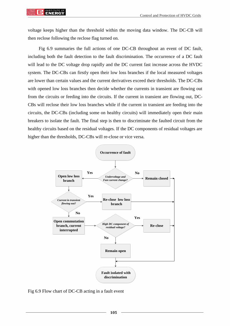
Control and Protection of HVDC Grids
105
voltage keeps higher than the threshold within the moving data window. The DC-CB will
then reclose following the reclose flag turned on.
Fig 6.9 summaries the full actions of one DC-CB throughout an event of DC fault,
including both the fault detection to the fault discrimination. The occurrence of a DC fault
will lead to the DC voltage drop rapidly and the DC current fast increase across the HVDC
system. The DC-CBs can firstly open their low loss branches if the local measured voltages
are lower than certain values and the current derivatives exceed their thresholds. The DC-CBs
with opened low loss branches then decide whether the currents in transient are flowing out
from the circuits or feeding into the circuits. If the current in transient are flowing out, DC-
CBs will reclose their low loss branches while if the current in transient are feeding into the
circuits, the DC-CBs (including some on healthy circuits) will immediately open their main
breakers to isolate the fault. The final step is then to discriminate the faulted circuit from the
healthy circuits based on the residual voltages. If the DC components of residual voltages are
higher than the thresholds, DC-CBs will re-close or vice versa.
Occurrence of fault
Undervoltage and
Fast current change?
Current in transient
flowing out?
High DC component of
residual voltage?
Open commutation
branch, current
interrupted
Re-close low loss
branch
Re-close
Fault isolated with
discrimination
Open low loss
branch Remain closed
Remain open
Yes No
Yes
No
Yes
No
Fig 6.9 Flow chart of DC-CB acting in a fault event

Control and Protection of HVDC Grids
106
6.8 SIMULATION RESULTS
6.8.1 TEST SYSTEM
The protection algorithm is tested on a 4-converter, symmetric monopole DC system
rated at +/-200 kV. This system is meshed by three OHLs and one cable (See Fig 6.10). DC-
CBs are located at both ends of each DC line. The entire system is high impedance ground at
its DC side.
Converters VSC1 and VSC2 are under the alternative DC voltage droop control while
converters VSC3 and VSC4 are in the power control mode.
OHL12(200km)
Cable34(200km)
OHL41(150km)
OHL23(100km)
VSC1 VSC2
VSC3VSC4
B1-2
B1
-4
B2-1
B2
-3B
3-2
B3-4B4-3
B4
-1
Fig 6.10 One line diagram of meshed DC test system Power Component
6.8.2 MODELLING OF DC COMPONENTS
All the OHLs and cables are represented using the frequency dependent model
provided in PSCAD/EMTDC. The conductor data (Type AAAC-806-A4-61) and ground
wire data (Type AFL CC-75-528) that have been used for OHL modelling are given in Table
6-2 [117][118]. The structure of tower is shown in Fig 6.11 [119].
The conductor data and material used for cable modelling are shown in Table 6-3,
[121] (PSCAD’s view shown in Fig 6.12). The general design of the cable cross-section is
derived from a real 150 kV XLPE VSC-HVDC submarine cable. The cross-section was
scaled up to a 320 kV cable respecting the diameter of the copper conductor, while keeping
the electric field stress (cold condition) similar [120].
All DC-CBs are modelled as simplified hybrid DC breakers [114]. They have a
current limit reactor rated at 0.1 H connected in series to limit the rate of rise of current. A

Control and Protection of HVDC Grids
107
surge arrester bank rated at 300 kV (1.5 p.u) is installed in parallel to absorb the fault energy
stored in DC system.
All converters are represented by MMC equivalent models developed in [122].
Table 6-2 PARAMETER FOR THE CONDUCTOR AND THE GROUND WIRE
Conductor Data
Type AAAC-806-A4-61
Total bundled sub-conductors 3
Bundle Spacing 0.457 m
DC resistance 0.036 ohm/km
Outside diameter 0.0381 m
Sag 19 m
Ground wire Data
Type AFL CC-75-528
Number of ground wire 1
DC resistance 0.034 ohm/km
Outside diameter 0.0165 m
Sag 19 m
Table 6-3 CONDUCTOR DATA AND GROUND WIRE DATA OF OHL MODEL
Layer Material Outer Radius
(mm)
Resistivity
(Ωm)
Rel.
permittivity
Rel.
permeability
Core Copper 21.4 1.72×10⁻⁸
1 1
Insulation XLPE 45.9 - 2.3 1
Sheath Lead 49.4 2.2×10⁻⁷
1 1
Insulation XLPE 52.4 - 2.3 1
Armour Steel 57.9 1.8×10⁻⁷
1 10
Insulation PP 61.0 - 2.1 1

Control and Protection of HVDC Grids
108
6.2
m2
0'4
'’
15.0 m(49'3'’)
6.0
m(1
9'8
'’)
45
.2 m
(14
8.3
')
33
.0 m
(10
8'3
'’)
4 GUYS9/16'’ EACHDOUBLE LOOP
Tower Weight5.300 Kg (12.000 lbs)
Guy Footprint
50 m×41 m (164'×135')
1.8 m(5'11'’)
Fig 6.11 Structure of the OHL tower
Fig 6.12 Configuration of cable modelling in PSCAD/EMTDC

Control and Protection of HVDC Grids
109
6.8.3 CASE STUDIES
Three cases are presented to show the effectiveness of Open Grid on protecting DC
systems. The thresholds setting of protection criteria and converter control parameter of
MMC-VSCs are given in Table 6-4.
Table 6-4 THRESHOLDS OF PROTECTION AND CONTROL SETTING OF VSCS
The sign convention of current flowing in both poles is shown in Fig 6.13.
Positive Pole
Negative Pole
Ia+ Ib+
Ia- Ib-
Fig 6.13 Sign convention of current in both poles
CASE 1- Pole to Pole Fault on OHL12
A solid pole to pole fault is applied at the middle point of OHL12 at 10 ms. Fig 6.14 (a)
and Fig 6.14 (b) show the voltage and current profiles of the positive pole. The voltage and
current profiles of the negative pole are symmetric to positive pole for a pole to pole fault (i.e.
same magnitude but different signs) and thus are not given. The fault is detected within 0.85
ms and then DC-CBs at both ends of the faulted section open (see Fig 6.14 (c)). The fault
current is thus fast interrupted and limited within 1.5 p.u. Thereafter, the discrimination is
achieved within 7 ms when the DC-CBs on healthy circuit all re-close. Fig 6.15 (a) to Fig
6.15 (c) shows the diagrams of integrations of current transient and current derivatives. Since
Components Items Description
Fault detection DC voltage 𝑉𝑑𝑐 < 150 kV Current derivative 𝑑𝑖𝑑𝑐
𝑑𝑡> 240 A/ms
Discrimination DC component of
residual voltage 𝑉𝑜 > 50 kV
Integration of current
transient 𝑄m > 0 C
Control of VSC1 and
VSC2
Load reference set
point (LRSP) 𝐿𝑅𝑆𝑃 = 400 𝑘𝑉
Current order 𝐼𝑜𝑟𝑑 = 2 𝑘𝐴
Droop characteristic 𝑘 = −6.25 𝑘𝐴/𝑘𝑉
Control of VSC3 and
VSC4
Power order 𝑃𝑜𝑟𝑑 = −800 𝑀𝑊

Control and Protection of HVDC Grids
110
the fault occurs at the middle of OHL12, the currents at B1-2 and B2-1 tend to infeed the
faulted point at the same time. The integrations of current in transient before DC-CBs
opening are thus positive at both ends. Meanwhile, DC-CBs at OHL23 and OHL41 also
generate open signals by detecting undervoltages and fast change of currents. B4-1 and B2-3
are then temporarily open their low loss branches since the integrations of current in transient
at these two points are positive. B1-4 and B3-2 however immediately receive re-close signals
by obtaining negative integrations of current transient s and thus stop opening.
Fig 6.14 Pole to pole fault on OHL12: (a) DC voltage; (b) DC current; (c) tripping timings
of DC-CB
10 110 210 310-400
-200
0
200
400
Time (ms)
DC
voltage (
kV
)
B1-2B2-1B2-3B3-2B3-4B4-3B1-4B4-1
10 110 210 310
-2
-1
0
1
2
Time (ms)
DC
curr
ent
(kA
)
B1-2B2-1B2-3B3-2B3-4B4-3B1-4B4-1
10 15 20Time (ms)
Trippin
g s
ignal
B1-2B2-1B2-3B3-2B3-4B4-3B1-4B4-1
(a)
(b)
(c)

Control and Protection of HVDC Grids
111
Fig 6.16 (a) to Fig 6.16 (c) shows the zoomed in voltages and their extracted DC
components. The DC components of voltages at the faulted section equal to zero and B1-2,
B2-1 keep open. The discrimination is achieved when B3-2 and B4-1 re-close based on high
DC components of residual voltages (i.e. >50kV) within the data window.
The benefits of using Open Grid are demonstrated by the extremely fast open of DC-
CBs and the fault current is limited within 1.5 p.u. This reduces the rating of current breaking
of DC-CBs. It also could help the selection of smaller current reactor to be used within DC-
CBs.
Fig 6.15 Integration of current transient and current derivatives at: (a) OHL12; (b) OHL23;
(c) OHL14
-20
0
20
Q (
C)
10 10.2 10.4 10.6 10.8 110
100020003000
Time (ms)
di/d
t (A
/ms)
B1-2
B2-1
-2000
200
Q (
C)
10 11 12 13
-5000
500
Time (ms)
di/dt
(A/m
s)
B2-3
B3-2
-300
-150
0
150
Q (
C)
10 11 12 13-2000
0
2000
Time (ms)
di/d
t (A
/ms)
B1-4
B4-1
(a)
(b)
(c)
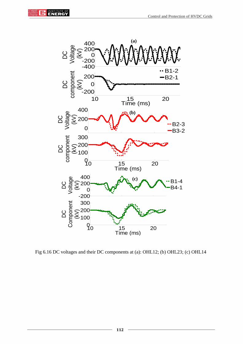
Control and Protection of HVDC Grids
112
Fig 6.16 DC voltages and their DC components at (a): OHL12; (b) OHL23; (c) OHL14
-400-200
0200400
DC
V
olta
ge
(kV
)
10 15 20
-200
0
200
Time (ms)
DC
com
ponent
(kV
)
B1-2
B2-1
0
200
400
DC
Volta
ge
(kV
)
10 15 200
100
200
300
Time (ms)
DC
com
ponent
(kV
)
B2-3
B3-2
-200
0
200
400
DC
Volta
ge
(kV
)
10 15 200
100
200
300
Time (ms)
DC
Com
ponent
(kV
)
B1-4
B4-1
(a)
(b)
(c)

Control and Protection of HVDC Grids
113
Fig 6.17 Pole to pole fault on Cable34: (a) DC voltage; (b) DC current; (c) tripping
timings of DC-CBs
CASE 2- Pole to Pole Fault on Cable34
A pole to pole fault occurs at the middle of Cable34 and the results are given as Fig
6.17 (a) to Fig 6.17 (c). From Fig 6.17 (c) it can be seen that the fault is detected and
discriminated within 1 ms. B3-4 and B4-3 open simultaneously since the electrical distances
to both cable ends are the same. All the DC-CBs on healthy circuits remain closed and thus
the discrimination is achieved simultaneously when the fault is isolated. This indicates that
within the Open Grid protection strategy, it is also possible that discrimination can be
achieved while only DC-CBs on faulted circuits fast open. This is very likely to happen in a
more capacitive transmission system (e.g. cables) where events of fault will cause much less
oscillation of voltages.
10 110 210 310
0
100
200
Time (ms)
DC
volta
ge (
kV)
B1-2B2-1B2-3B3-2B3-4B4-3B1-4B4-1
10 110 210 310
-2
-1
0
1
2
Time (ms)
DC
curr
ent
(kA
)
B1-2B2-1B2-3B3-2B3-4B4-3B1-4B4-1
10 15 200
5
10
15
Time (ms)
Trippin
g s
ignal
B1-2B2-1B2-3B3-2B3-4B4-3B1-4B4-1
(a)
(b)
(c)

Control and Protection of HVDC Grids
114
CASE 3- Pole to Ground Fault on OHL12
A positive pole to ground fault with an impedance of 300 ohm is applied at the middle
point of OHL12 at 10 ms. Results are shown in Fig 6.18 to Fig 6.20.
Fig 6.18 Pole to ground fault on OHL12: (a) DC voltage; (b) DC current; (c) tripping
timings of DC-CBs
Since the DC system is high impedance grounded at the DC side, the fault is mainly
contributed by the discharging current of transmission lines circulating to the ground during
transient time. The voltages at the faulted section drop to zero (see Fig 6.20) and the
integration of pre-tripping current at both its line ends are positive (i.e. indicating an internal
-2000
200400
+ P
ole
voltage
(kV
)
B1-2B2-1B2-3B3-2B3-4B4-3B1-4B4-1
10 110 210 310
-400
-200
0
200
Time (ms)
- P
ole
voltage
(kV
)
-2
0
2
+ P
ole
curr
ent
(kA
)
10 110 210 310-2
0
2
Time (ms)
- P
ole
curr
ent
(kA
)
B1-2B2-1B2-3B3-2B3-4B4-3B1-4B4-1
10 15 20Time (ms)
Trippin
g s
ignal
B1-2B2-1B2-3B3-2B3-4B4-3B1-4B4-1
(a)
(b)
(c)

Control and Protection of HVDC Grids
115
fault) (see Fig 6.19). Therefore, the DC-CBs on the faulted section (positive pole) open and
will not re-close. B3-2 and B4-1 have negative integration of currents and will only
temporarily open their low loss branches. The discrimination is achieved within 7.5 ms when
B2-3 re-closes based on high DC components of residual voltage. The speed of interrupting a
high impedance fault is also very fast using Open Grid. The robustness of discriminating
different types and of fault is guaranteed by enabling the re-closure function of DC-CBs.
Fig 6.19 Integration of current transient and current derivatives at: (a) OHL12; (b) OHL23;
(c) OHL14
10 10.5 11
0
200
400
Time (ms)
di/d
t (kA
/ms)
0
10
20
Q (
C)
B1-2
B2-1
-100
0
100
Q (
C)
10 11 12-1000
0
1000
Time (ms)
di/d
t (kA
/ms)
B2-3
B3-2
-400
-200
0
200
Q (
C)
10 11 12 13
2000
0
-2000
Time (ms)
di/d
t (kA
/ms)
B1-4
B4-1
(a)
(b)
(c)

Control and Protection of HVDC Grids
116
Fig 6.20 DC voltages and their DC components at (a): OHL12; (b) OHL23; (c) OHL14
6.8.4 SUMMARY
The speed of DC network protection is of great importance. This chapter has
investigated the feasibility of using Open Grid within which DC-CBs trip rapidly based on
local measurements to isolate the fault and then achieve discrimination afterwards. This
change of protection sequence avoids the delay caused by discrimination for isolating a fault
and thus reduces the time for fault isolation. The interruption of smaller fault current may
bring down the size of protection devices. The use of Open Grid also facilitates the design of
-500
0
500
DC
volta
ge(k
V)
10 15 20-100
0100200300
Time (ms)
DC
com
pone
nt(k
V)
B1-2
B2-1
0
200
400
DC
volta
ge(k
V)
10 15 20100
200
300
Time (ms)
DC
com
pone
nt(k
V)
B2-3
B3-2
0
200
400
DC
volta
ge
(kV
)
10 15 200
100
200
300
Time (ms)
DC
com
ponent
(kV
)
B1-4
B4-1
(a)
(b)
(c)

Control and Protection of HVDC Grids
117
fault detection algorithm. Local measured voltages and currents can be used directly to detect
a fault. This may lead the DC-CBs on some healthy sections to temporarily open.
Two criteria for fault discrimination have been used to ensure fast re-closure of DC-
CBs on healthy sections. Firstly, the integration of current in transient can be used as one
criterion for fault discrimination. The current in transient on faulted sections will always flow
internally, towards the faulted point. However, the current in transient of healthy circuits will
flow outside from one or both line ends. Therefore, the DC-CBs can either reclose their low
loss branch or open the main breakers to isolate the fault based on the sign of integration of
current in transient. Secondly, the residual voltage is used for the re-closure of DC-CBs that
open their main breakers. The DC components of residual voltages on healthy circuits will
retain at non-zero values while that on the faulted section will always damp to zero.
Therefore, the DC-CBs can either reclose or keep open to achieve the discrimination.
Different tests have been undertaken to demonstrate the ability of the Open Grid
protection method to detect and discriminate different types of DC faults using
PSCAD/EMTDC. The results have shown that the Open Grid can successfully detect and
discriminate all DC faults in different fault conditions in a meshed DC grid.

Control and Protection of HVDC Grids
118
Chapter 7
7. Conclusion and Future
Work
7.1 CONCLUSION
7.1.1 HVDC GRID CONTROL
HVDC grids have been made practical with the introduction of the VSC. One major
challenge for building HVDC grids is the development of the control schemes of HVDC
grids.
This thesis has contributed to develop a method known as ACC for the control of
HVDC grids. With this method, alternative droop characteristics are used for each converter.
Within the active range of such characteristics high droops are used while outside the active
range, flat droops are implemented.
It has been found that the high droops within the active range can significantly reduce
the converter current error and hence increase the accuracy of DC current flow. Moreover,
the flat droops outside the active range can stabilise DC voltage. Therefore, it is concluded
that with the ACC method, multiple converters can share the responsibility of regulating DC
voltage while the converter current can be precisely regulated.
Another main finding is that the use of alternative droop and power control within
converters could cause multiple cross-over of the control characteristics. For those converters
using ACC, the design of the droop values within the active range must be smaller than the
slope of power curves (of those power controlled converters) and hence the multiple
operation points can be avoided.
A hardware 4-terminal HVDC test rig has been designed and configured to demonstrate
the implementation of ACC and to access its control performance. At the DC side of the rig,
four converters are connected in a star configuration using cable representations. At the AC

Control and Protection of HVDC Grids
119
side of the rig, two converters are connected to the laboratory AC power supply which
emulates strong AC grid while the other converters are connected to motor-generator units
which represents the offshore wind farms. Moreover, digital simulations using
PSCAD/EMTDC are also undertaken to demonstrate the ACC.
Comparison of both the simulation and experimental results are made, showing good
agreement. Both results show that the use of alternative droop characteristics within ACC can
increase the accuracy of DC current control. In the first case study, the current error function
can reduced the current error by 12.5%. In the second case study, the converter with Type 2
control regulates its current much more precisely in the condition that wind power changes.
In addition, the multiple-cross over of control characteristics has also been
demonstrated. It has been found that when alternative droop characteristics are used for the
import converter and power control is used for export converter, the DC system will not
operate at the desirable operating point. In contrast, when the conventional droop is used for
the import converter or the alternative droop characteristics are used for the export converter,
there is no multiple-cross over of control characteristics. Therefore, the droop gain of
alternative droop characteristics should be carefully designed using the method developed in
Chapter 3 to avoid the multiple-cross over of control characteristics.
Furthermore, the control coordination of converters and DC power flow controller (DC-
PFC) on optimising the wind power delivery has also been studied. The DC power flow of
HVDC grids integrated with DC-PFCs is described. An analytical expression is derived
which can be used to estimate the impact of changing the control orders of converters and
DC-PFCs. It is found that the changing the control orders of converters will not influence the
branch power that controlled by DC-PFCs. However, by change the control orders of DC-
PFCs will cause the power and voltages of droop controlled converter to vary. A method for
optimising the wind power delivery by re-dispatching the control orders of converters and
DC-PFCs has also been developed. Case studies are undertaken, showing that by re-
dispatching the control orders, the wind power delivered to shore can be increased. When the
wind power generation is low, the control orders can be re-dispatched to reduce system
power losses. When power generation is high, the control orders can then be re-dispatched to
reduce the wind power curtailment.

Control and Protection of HVDC Grids
120
7.1.2 HVDC GRID PROTECTION
The HVDC grid protection is a key challenge for the development of HVDC grids. A
protection method - Open Grid has been developed to use DC-CBs to fast isolate DC faults in
HVDC grids. The developed Open Grid allows multiple DC-CBs to interrupt the fault current
based on local measurements of voltage (and current) and then reclose the DC-CBs on
healthy circuits to achieve discrimination. As a result, the speed of fault current interruption
can be significantly reduced. Therefore, the current rating required for DC-CBs can also be
reduced.
The fault detection principle is developed based on a combination of local voltage and
current derivatives. Consequently, DC-CBs can open when detect DC voltages drop below
the pre-set thresholds and the rates of currents increasing are higher than their thresholds. In
this way, the fault can be isolated very quickly.
The discrimination principle is developed based on the residual DC voltage on opened
circuits and the currents in transient. The DC-CB can reclose if it detects the DC component
of local residual DC voltage is maintained at a non-zero value. Conversely, the DC-CB will
keep open if the DC component of local residual DC voltage is zero. The measurements of
currents in transient are also used to guarantee the discrimination. The currents in transient of
faulted section will flow internally towards the faulted point while that of healthy sections
will flow externally at least one end. Therefore, by analysing the direction of the current
flowing in transient, the DC-CB can reclose correctly and the discrimination can be ensured.
A four-terminal mashed HVDC grid model is built in PSCAD/EMTDC to demonstrate
the effectiveness of using Open Grid for HVDC grid protection. Different tests with various
fault types, locations and fault impedances are undertaken to assess the protection
performance. The tests show that the Open Grid can fast detect and discriminate all the DC
faults in the meshed HVDC grid.
7.2 FUTURE WORK
The following future work can be conducted to extend the work described in this thesis:
7.2.1 PROTECTION OF NON-PERMANENT DC FAULT
DC overhead lines (OHLs) are important candidates to be integrated within HVDC
grids. The OHLs are subjected to non-permanent DC faults and hence future work on HVDC

Control and Protection of HVDC Grids
121
protection should consider the detection and discrimination of different types of non-
permanent DC faults.
In a DC fault event, a desirable protection method should be able to fast discriminate
the faulted circuit while also identify if a DC fault is permanent or non-permanent. Moreover,
auto-reclosing of DC-CBs may be needed to recover the faulted OHL when a non-permanent
fault no longer exists. The proposed Open Grid has already developed the algorithm for the
auto-reclosing of DC-CBs (based on residual DC voltage and current transient) and hence
facilitates the further development of the protection method. However, additional criteria and
approaches may be needed to discriminate a non-permanent fault from a permanent fault. For
example, post to the isolation of a non-permanent fault, the fault could last for hundreds of
milliseconds and the DC voltage on the faulted OHL could drop to zero. The DC-CBs may
have to temporarily reclose to recharge the faulted OHL for a short period and then open
again. If the voltage of the recharged OHL is maintained at a non-zero level then it can be
determined that the DC fault is non-permanent and the DC-CBs will reclose to restore the
system. In contrast, the voltage of the recharged OHL drops to zero again, then the DC fault
is permanent and the DC-CBs will remain open.
7.2.2 PROTECTION OF DC OHLS SHARING A COMMON TOWER
The future reinforcement of transmission could lead more AC OHLs to be used as DC
OHLs and thus to increase the transmission capacity. A double-circuit three-phase AC OHL
transmission system can be configured as three symmetric monopole DC OHL transmission
systems. These DC OHLs are electromagnetic coupled as they are sharing one common tower.
A DC fault, in particular, a pole to ground fault occurs at one OHL will have an impact on the
DC voltage and current at other healthy OHLs due to the electromagnetic coupling. These
could further lead to the maloperations of the DC-CBs on these healthy OHLs.
Therefore, future work should consider the development of methods to discriminate the
fault on an OHL sharing the same tower with other OHLs. The electromagnetic coupling
between OHLs should be analysed in detail with the consideration of different tower
configurations and conductor parameters.

Control and Protection of HVDC Grids
122
References
[1] National Grid, “UK future energy scenarios,” National Grid Report, 2011.
[2] National Grid, “ENSG ‘Our Electricity Transmission Network: A Vision For 2020,”
Updated Full Report, 2012.
[3] Office for Gas and Electricity Markets (OFGEM), “GB offshore transmission, Investment
Opportunity – Tender Round 2,” Tender 2 Report, 2012.
[4] National Grid, “Round 3 offshore wind farm connection study,” Technical Report prepared
for The Crown Estate, Version 1, 2012
[5] TRADEWIND. Wind power integration and exchange in the Trans-European power
markets [online]. Available:
https://ec.europa.eu/energy/intelligent/projects/en/projects/tradewind.
[6] OffshoreGrid, “Offshore electricity grid infrastructure in Europe,” Final report, 2011.
[7] North Sea Countries’ Offshore Grid Initiative (NSCOGI), “Political declaration on energy
cooperation between the North Seas Countries,” Political declaration, 2012.
[8] National Grid, “Offshore development information statement,” National Grid Report, 2010.
[9] Red Eléctrica de España,etc.”TWENTIES Project”, Final Report, 2013.
[10] Cardiff University, etc. Multi-terminal DC grid for offshore wind (MEDOW) [Online].
Available: http://sites.cardiff.ac.uk/medow/
[11] Friends of the Supergrid, “Roadmap to the supergrid technologies”, Final Report,
March 2012
[12] European Network of Transmission System Operators for Electricity (ENTSO-E),
“Research & development roadmap 2103-2022,” Research and Development Report, 2012.
[13] CIGRE Working Group B4.52, “HVDC grid feasibility study,” Technical Report 533,
2013.
[14] CIGRE Working Group B4 56, “Guidelines for the preparation of connection
agreements or Grid Codes for HVDC Grids,” Working Group Form, 2011.
[15] CIGRE Working Group B4.57, “Guide for the development of models for HVDC
converters in a HVDC grid,” Technical Brochure 604, 2014.

Control and Protection of HVDC Grids
123
[16] CIGRE Working Group B4.58, “Devices for load flow control and methodologies for
direct voltage control in a meshed HVDC grid,” Working Group Form, 2011.
[17] CIGRE Working Group B4.59, “Control and protection of HVDC grids,” Working
Group Form, 2011.
[18] CIGRE Working Group B4.60, “Designing HVDC grids for optimal reliability and
availability performance,” Working Group Form, 2011.
[19] N. Seki, "Field testing of 53 MVA three-terminal DC link between power systems using
GTO converters," IEEE Power Engineering Society Winter Meeting, Singapore, 2000, pp.
2504-2508.
[20] Alstom. South West Link: Balancing the power supply between central and southern
Sweden with HVDC [Online]. Available:
http://www.gegridsolutions.com/alstomenergy/grid/Global/OneAlstomPlus/Grid/PDF/Super
grid/SouthWest%20link%20HVDC%20project-epslanguage=en-GB.pdf
[21] Z. Alaywan, "The Tres Amigas Superstation: Linking renewable energy and the nation's
grid (July 2010)," IEEE PES General Meeting, Minneapolis, MN, 2010, pp. 1-5.
[22] X. Li, Z. Yuan, J. Fu, Y. Wang, T. Liu and Z. Zhu, "Nanao multi-terminal VSC-HVDC
project for integrating large-scale wind generation," IEEE PES General Meeting |
Conference & Exposition, National Harbor, MD, 2014, pp. 1-5.
[23] C. Li, X. Hu, J. Guo and J. Liang, "The DC grid reliability and cost evaluation with
Zhoushan five-terminal HVDC case study," 50th International Universities Power
Engineering Conference (UPEC), Stoke on Trent, UK, 2015, pp. 1-6.
[24] Committee Energy and Climate Change Committee, “A European Supergrid”, Seventh
Report of Session 2010–12, 2011
[25] C. D. Barker, R. S. Whitehouse, A. G. Adamczyk, and M. Boden, “ Designing fault
tolerant HVDC networks with a limited need for HVDC circuit breaker operation,” Cigre
2014, Paris, France, 2014, pp. 1-11.
[26] A. Gustafsson, M. Saltzer, A. Farkas, H. Ghorbani, T. Quist, and M. Jeroense, “The new
525 kV extruded HVDC cable system,” ABB Technical Paper, 2014.
Control and Protection of HVDC Grids
124
[27] R. Rudervall, J. P. Charpentier and R. Sharma, “High voltage direct current (HVDC)
transmission systems technology review paper,” Energy Week 2000, Washington, D.C,
USA, 2000, pp. 1-17.
[28] M. Szechtman, T. Wess and C. V. Thio, "A benchmark model for HVDC system
studies," International Conference on AC and DC Power Transmission, London, UK, 1991,
pp. 374-378.
[29] L. C. O. de Oliveira, W. M. Borges, J. B. de Souza and L. L. Ravagnani, "DC and AC
Side Harmonics in CCC Converters," Power Engineering Society Conference and
Exposition in Africa, Johannesburg, Gauteng, 2007, pp. 1-5.
[30] ABB. Gotland HVDC light [Online]. Available:
http://new.abb.com/systems/hvdc/references/gotland-hvdc-light
[31] B. R. Andersen, L. Xu and K. T. G. Wong, "Topologies for VSC transmission," Seventh
International Conference on AC-DC Power Transmission, 2001, pp. 298-304.
[32] M. Pereira, D. Retzmann, J. Lottes, M. Wiesinger and G. Wong, "SVC PLUS: An MMC
STATCOM for network and grid access applications," 2011 IEEE Trondheim PowerTech,
Trondheim, Norway, 2011, pp. 1-5.
[33] Simon P. Teeuwsen, “Modeling the Trans Bay Cable Project as Voltage-Sourced
Converter with Modular Multilevel Converter Design” 2011 IEEE Power and Energy
Society General Meeting, Detroit, MI, USA, 2011, pp 1-8.
[34] A. Yazdani and R. Iravani, “Grid-imposed frequency VSC system: control in dq-frame.”
in Voltage-source converters in power systems: modeling, control, and application, 1st ed.
Hoboken, New Jersey: John Wiley & Sons, 2010, ch. 8, pp. 204-245.
[35] G. S. Konstantinou and V. G. Agelidis, "Performance evaluation of half-bridge cascaded
multilevel converters operated with multicarrier sinusoidal PWM techniques," 4th IEEE
Conference on Industrial Electronics and Applications, Xi'an, China, 2009, pp. 3399-3404.
[36] P. M. Meshram and V. B. Borghate, "A Simplified Nearest Level Control (NLC)
Voltage Balancing Method for Modular Multilevel Converter (MMC)," IEEE Transactions
on Power Electronics, vol. 30, no. 1, pp. 450-462, Jan. 2015.
[37] H. Saad, X. Guillaud, J. Mahseredjian, S. Dennetière and S. Nguefeu, "MMC Capacitor
Voltage Decoupling and Balancing Controls," IEEE Transactions on Power Delivery, vol.
30, no. 2, pp. 704-712, April 2015.

Control and Protection of HVDC Grids
125
[38] P. M. Meshram and V. B. Borghate, "A novel voltage balancing method applied to
direct control strategy of MMC-HVDC system," 2012 International Conference on
Advances in Engineering, Science and Management (ICAESM), Nagapattinam, Tamil Nadu,
2012, pp. 448-452.
[39] P. Münch, D. Görges, M. Izák and S. Liu, "Integrated current control, energy control
and energy balancing of Modular Multilevel Converters," 36th Annual Conference on IEEE
Industrial Electronics Society (IECON 2010), Glendale, AZ, 2010, pp. 150-155.
[40] F. Yu, W. Lin, X. Wang and D. Xie, "Fast Voltage-Balancing Control and Fast
Numerical Simulation Model for the Modular Multilevel Converter," IEEE Transactions on
Power Delivery, vol. 30, no. 1, pp. 220-228, Feb. 2015.
[41] A. Lesnicar and R. Marquardt, "An innovative modular multilevel converter topology
suitable for a wide power range," 2003 IEEE Bologna Power Tech Conference Proceedings,
Bologna, Italy, 2003, pp. 1-6.
[42] M. Guan, Z. Xu and H. Li, "Analysis of DC voltage ripples in modular multilevel
converters," 2010 International Conference on Power System Technology (POWERCON),
Hangzhou, China, 2010, pp. 1-6.
[43] Q. Tu, Z. Xu and J. Zhang, “Circulating current suppression control in Modular
Multilevel Converter,” IECON 2010-30th Annual Conference on IEEE Industrial
Electronics Society, Glendale, AZ, 2010, pp. 1-6.
[44] D. V. Hertem, O. Gomis-Bellmunt and J. Liang, “ HVDC technology overview,” in
HVDC Grids for Offshore and Supergrid of the Future, 1st ed. Hoboken, New Jersey: John
Wiley & Sons, 2016, ch. 3, sec. 3.6, pp. 72-76.
[45] Z. H. Liu, L. Y. Gao, Z. L. Wang, J. Yu, J. Zhang, and L. C. Lu, “R&D progress of
±1100 kV UHVDC technology,” CIGRE paper B4_201_2012, 2012, pp. 1–6.
[46] R. Liu, “Long-distance DC electrical power transmission,” IEEE Electrical Insulation
Magazine, vol. 29, no. 5, pp. 37-40, 2013.
[47] G. Chen, M. Hao, Z. Xu, A. Vaughan, J. Cao and H. Wang, “Review of high voltage
direct current cables”, CSEE J. of Power and Energy System, vol. 1, no. 2, pp. 9-21, 2015.
[48] E. Houston, “Western HVDC link environmental report, volume 1: Non-technical
summary: Marine cable route,”, Western Link project website, 2011 [Online]. Available:

Control and Protection of HVDC Grids
126
http://spng.opendebate.co.uk/files/_ER_MCR_NTS__STANDALONE_reduced_file_size.p
df
[49] T. L. Hanley, R. P. Burford, R. J. Fleming, K. W. Barber, “A general review of
polymeric insulation for use in HVDC cables”, IEEE Electrical Insulation Magazine, vol.
19, no. 1, pp. 13-24, 2003.
[50] B. Pauli, G. Mauthe, E. Ruoss, G. Ecklin, J. Porter and J. Vithayathil, "Development of
a high current HVDC circuit breaker with fast fault clearing capability," IEEE Transactions
on Power Delivery, vol. 3, no. 4, pp. 2072-2080, Oct 1988
[51] A. N. Greenwood and T. H. Lee, "Theory and Application of the Commutation Principle
for HVDC Circuit Breakers," IEEE Transactions on Power Apparatus and Systems, vol.
PAS-91, no. 4, pp. 1570-1574, July 1972.
[52] M. M. Walter, “ Switching arcs in passive resonance HVDC circuit breakers,” Doctor of
Science Thesis, 2013.
[53] K. Tahata, S. Oukaili, K. Kamei, D. Yoshida, Y. Kono, R. Yamamota and H. Ito,
“HVDC circuit breakers for HVDC grid applications”, 11th IET International Conference
on AC and DC Power Transmission, Birmingham, UK, 2015, pp. 1-9.
[54] J. Magnusson, R. Saers, L. Liljestrand and G. Engdahl, "Separation of the Energy
Absorption and Overvoltage Protection in Solid-State Breakers by the Use of Parallel
Varistors," IEEE Transactions on Power Electronics, vol. 29, no. 6, pp. 2715-2722, June
2014.
[55] G. F. Tang, Z. Y. He, H. Pang, X. M. Huang and X. P. Zhang, "Basic topology and key
devices of the five-terminal DC grid," in Power and Energy Systems, CSEE Journal of
power and energy systems , vol.1, no.2, pp.22-35, June 2015
[56] M. Callavik, A. Blomberg, J. Hafner and B. Jacobson, “The hybrid HVDC breaker: an
innovation breakthrough enabling reliable HVDC grids,” ABB Grid System Technical
Paper, 2012, pp. 1-10.
[57] C. D. Barker, R. S. Whitehouse, “Autonomous converter control in a multi-terminal
HVDC system”, AC and DC Power Transmission, 2010, Oct. 2010
[58] W. Lu, and B. T. Ooi, “Multi-terminal DC transmission system for wind-farms,” IEEE
Power Engineering Society Winter Meeting, Columbus, US, 2001, pp.1-6.
Control and Protection of HVDC Grids
127
[59] W. Lu and B.T. Ooi, “Optimal acquisition and aggregation of offshore wind power by
multiterminal voltage-source HVDC,” IEEE Transactions on Power Delivery, vol. 18, no. 1,
pp. 201–206, Jan. 2003.
[60] W. Lu and B. T. Ooi, “Premium Quality Power Park Based on Multi-Terminal HVDC,”
IEEE Transactions on Power Delivery, vol. 20, no. 2, pp.978-983, April 2005.
[61] K. Zhou, X. Fu, M. Cheng, X. Zhu, W. Wang and T. Wang, “Topologies and Control of
VSC-HVDC Systems for Grid Connection of Large-Scale Off-Shore Wind Farms,”
International Conference on Electrical Machines and Systems, Wuhan, China, 2008, pp.1-5.
[62] W. Lu and B. T. Ooi, “DC Overvoltage Control During Loss of Converter in
Multiterminal Voltage-Source Converter-Based,” IEEE Transactions on Power Delivery,
vol. 18, no. 3, pp. 915-920, July, 2003.
[63] T. Nakajima, S. Irokawa, “A control System for HVDC Transmission by Voltage Sourced
Converters,” IEEE Power Engineering Society Summer Meeting, Alberta, Canada, 1999, pp.
1113-1119.
[64] V. Mier, P. G. Casielles, J. Coto and L. Zeni, “Voltage margin control for offshore multi-
use platform integration,” International Conference on Renewable Energies and Power
Quality, Santiago de Compostela, Spain, 2012, pp.982-987.
[65] T. M. Haileselassie, M. Molinas and T. Undeland, “Multi-Terminal VSC-HVDC System
for Integration of Offshore Wind Farms and Green Electrification of Platforms in the North
Sea,” Nordic Workshop on Power and Industrial Electronics, Otaniemi Espoo, Finland,
2008, pp.1-5.
[66] J. Zhu and C Booth, “Future Multi-Terminal HVDC Transmission Systems using Voltage
Source Converters,” 45th
Universities’ Power Engineering Conference, Cardiff, Wales,
2010, pp.1-6.
[67] R. T. Pinto, S. F. Rodrigues, P. Bauer and J. Pierik, "Comparison of direct voltage control
methods of multi-terminal DC (MTDC) networks through modular dynamic models,"
Power Electronics and Applications (EPE 2011), Proceedings of the 2011-14th European
Conference on, Birmingham, 2011, pp. 1-10.
[68] R. da Silva, R. Teodorescu and P. Rodriguez, "Power delivery in multi-terminal VSC-
HVDC transmission system for offshore wind power applications," 2010 IEEE PES

Control and Protection of HVDC Grids
128
Innovative Smart Grid Technologies Conference Europe (ISGT Europe), Gothenburg, 2010,
pp. 1-8.
[69] J. Liang, O. Gomis-Bellmunt, J. Ekanayake and N. Jenkins, “Control of multi-terminal
VSC-HVDC transmission for offshore wind power,” 13th
European Conference on Power
Electronics and Applications (EPE 2009), Barcelona, Spain, 2009, pp. 1-10.
[70] S. Zhou, J. Liang, J. Ekanayake and N. Jenkins, “Control of multi-terminal VSC-HVDC
transmission system for offshore wind power generation,” 2009 Proceedings of the 44th
Universities’ International Power Engineering Conference (UPEC 2009), Glasgow, UK,
2009, pp. 1-5.
[71] O. Gomis-Bellmunt, A. Egea-Alvarez, A. Junyent-Ferre, J. Liang, J. Ekanayake and N.
Jenkins, “Multiterminal HVDC-VSC for offshore wind power integration,” 2011 IEEE
Power and Energy Society General Meeting, San Diego, CA, 2011, pp.1-6.
[72] J. Liang, T. Jing, O. Gomis-Bellmunt, J. Ekanayake and N. Jenkins, “Operation and
Control of Multiterminal HVDC Transmission for Offshore Wind Farms.” IEEE
Transactions on Power Delivery, vol. 26, no. 4, pp. 2596-2604, October, 2011.
[73] T. M. Haileselassie and K. Uhlen, “Impact of DC Line Voltage Drops on Power Flow of
MTDC Using Droop Control,” IEEE Transactions on Power Systems, vol. 27, no. 3, pp.
1441-1449, August, 2012.
[74] C. D. Barker and R. Whitehouse, “Further developments in autonomous converter control
in a multi-terminal HVDC system,” 10th International Conference on AC and DC Power
Transmission (ACDC 2012), Birmingham, UK, 2012, pp. 1-6.
[75] Radiodetection. Cable and Cable Fault Locating -Part 3. [Online]. Available:
http://www.radiodetection.co.uk/doclib/SPX_3_Cable_and_cable_fault_locating___part_3_
en.pdf
[76] Brugg Cables. High Voltage XLPE Cable Systems -Technical User Guide. [Online].
Available: http://www.kpa.co.ke/InfoCenter/Tenders/Documents/Archives/Appendix ii
typical cable specs A 03_web_xlpe_guide_en.pdf.
[77] C. D. Barker and R. S. Whitehouse, "An alternative approach to HVDC grid protection,"
10th IET International Conference on AC and DC Power Transmission, Birmingham, UK,
2012, pp.1-6.
Control and Protection of HVDC Grids
129
[78] P. Bresesti, W. L. Kling, R. L. Hendriks and R. Vailati, "HVDC Connection of Offshore
Wind Farms to the Transmission System," IEEE Transactions on Energy Conversion, vol.
22, no. 1, pp. 37-43, March 2007.
[79] O. A. Giddani, G. P. Adam, O. Anaya-Lara and K. L. Lo, "Grid integration of offshore
wind farms using multi-terminal DC transmission systems (MTDC)", 5th IET International
Conference on Power Electronics, Machines and Drives (PEMD 2010), Brighton, UK,
2010, pp. 1-6.
[80] S. Henry, A. M. Denis and P. Panciatici, "Feasibility study of off-shore HVDC grids,"
IEEE PES General Meeting, Minneapolis, MN, 2010, pp. 1-5.
[81] U. Wijk, J. Lindgren, J. Winther, and S. Nyberg, “Dolwin1-Further achievements in
HVDC offshore connections,” EWEA Offshore 2013, Frankfurt, Germany, 2013, pp. 1-6.
[82] K. Johannesson, A. Gustafsson, J. Karlstrand, and M. Jeroense, “Light cables for long
distance grid connection,” 2009 European Offshore Wind Conference, Stockholm, Sweden,
2009, pp. 1-5.
[83] X. Jiang, Y. Jiang, X. Kong, “A Demonstration Project of Flexible DC Power
Transmission in Shanghai Nanhui Wind Power Station,” High Voltage Engineering, vo. 41,
no. 4, pp.1132-1139, Nov. 2014.
[84] O. Gomis-Bellmunt, J. Liang, J. Ekanayake, R. King, and N, Jenkins, “Topologies of
multiterminal HVDC-VSC transmission for large offshore wind farms,” Electric Power
System Research, vol. 81, no. 2, pp. 271-281, Feb. 2011.
[85] E. Veilleux and B.-T., Ooi, “Multi-Terminal HVDC Grid with Power Flow
Controllability,” CIGRE, 2012, pp. 1-12.
[86] N. Deng, P. Wang, X. P. Zhang, G. Tang and J. Cao, "A DC current flow controller for
meshed modular multilevel converter multiterminal HVDC grids," in CSEE Journal of
Power and Energy Systems, vol. 1, no. 1, pp. 43-51, March 2015.
[87] D. Jovcic, M. Hajian, H. Zhang and G. Asplund, "Power flow control in DC transmission
grids using mechanical and semiconductor based DC/DC devices," 10th IET International
Conference on AC and DC Power Transmission (ACDC 2012), Birmingham, UK, 2012, pp.
1-6.

Control and Protection of HVDC Grids
130
[88] E. Veilleux and B. T. Ooi, "Multiterminal HVDC With Thyristor Power-Flow
Controller," IEEE Transactions on Power Delivery, vol. 27, no. 3, pp. 1205-1212, July
2012.
[89] Q. Mu, J. Liang, Y. Li and X. Zhou, "Power flow control devices in DC grids," 2012
IEEE Power and Energy Society General Meeting, San Diego, CA, 2012, pp. 1-7.
[90] C. D. Barker and R. S. Whitehouse, "A current flow controller for use in HVDC grids,"
10th IET International Conference on AC and DC Power Transmission (ACDC 2012),
Birmingham, UK, 2012, pp. 1-5.
[91] W. Chen, X. Zhu, L. Yao, X. Ruan, Z. Wang and Y. Cao, "An Interline DC Power-Flow
Controller (IDCPFC) for Multiterminal HVDC System," IEEE Transactions on Power
Delivery, vol. 30, no. 4, pp. 2027-2036, Aug. 2015.
[92] C. D. Baker and R. S. Whitehouse, “Current flow controller,” US Patent Application,
2015/0180231 A1, 2015.
[93] P. Trodden, W.A. Bukhsh, A. Grothey, and K. M. McKinnon, “Optimization-Based
Islanding of Power Networks Using Piecewise Linear AC Power Flow”, IEEE Transactions
on Power System, vol. 29, no. 3, pp. 1212-1220, May. 2014.
[94] S. Wang, J. Liang A. Wen and C. Feng, “Cost and benefits analysis of VSC-HVDC
schemes for offshore wind power transmission,” Automation of Electric Power Systems, vol.
37, no. 13, pp. 36-43, 2013.
[95] A. Moawwad, M. S. El Moursi and W. Xiao, "A Novel Transient Control Strategy for
VSC-HVDC Connecting Offshore Wind Power Plant," IEEE Transactions on Sustainable
Energy, vol. 5, no. 4, pp. 1056-1069, Oct. 2014.
[96] J. Hu, L. Yu, F. Zhang and J. Lu, "Research on the DC faults in multi-terminal DC
transmission system on MMC," International Journal of Advanced Research in Electrical,
Electronics and Instrumentation Engineering, vol. 2, no. 5, pp. 2029-2036, May 2013.
[97] J. Sneath and A. D. Rajapakse, "DC Fault Protection of a Nine-Terminal MMC HVDC
Grid," 11th IET International Conference on AC and DC Power Transmission,
Birmingham, UK, 2015, pp. 1-8.
[98] M. K. Bucher, M. M. Walter, M. Pfeiffer and C. M. Franck, "Options for ground fault
clearance in HVDC offshore networks," 2012 IEEE Energy Conversion Congress and
Exposition (ECCE), Raleigh, NC, 2012, pp. 2880-2887.

Control and Protection of HVDC Grids
131
[99] C. M. Franck, "HVDC Circuit Breakers: A Review Identifying Future Research Needs,"
IEEE Transactions on Power Delivery, vol. 26, no. 2, pp. 998-1007, April 2011.
[100] L. Tang and B. T. Ooi, "Locating and Isolating DC Faults in Multi-Terminal DC
Systems," IEEE Transactions on Power Delivery, vol. 22, no. 3, pp. 1877-1884, July 2007.
[101] A. Adamczyk, C. D. Barker and H. Ha, "Fault detection and branch identification for
HVDC grids," 12th IET International Conference on Developments in Power System
Protection (DPSP 2014), Copenhagen, Denmark, 2014, pp. 1-6.
[102] K. D. Kerf et al., "Wavelet-based protection strategy for DC faults in multi-terminal VSC
HVDC systems," IET Generation, Transmission & Distribution, vol. 5, no. 4, pp. 496-503,
April 2011.
[103] J. Descloux, B. Raison and J. B. Curis, "Protection algorithm based on differential voltage
measurement for MTDC grids," 12th IET International Conference on Developments in
Power System Protection (DPSP 2014), Copenhagen, Denmark, 2014, pp. 1-5.
[104] Y. Zhang, N. Tai and B. Xu, "Fault Analysis and Traveling-Wave Protection Scheme for
Bipolar HVDC Lines," IEEE Transactions on Power Delivery, vol. 27, no. 3, pp. 1583-
1591, July 2012.
[105] X. Liu, A. H. Osman and O. P. Malik, "Hybrid Traveling Wave/Boundary Protection for
Monopolar HVDC Line," IEEE Transactions on Power Delivery, vol. 24, no. 2, pp. 569-
578, April 2009.
[106] J. Cheng, M. Guan, L. Tang, H. Huang, X. Chen and J. Xie, "Paralleled multi-terminal
DC transmission line fault locating method based on travelling wave," IET Generation,
Transmission & Distribution, vol. 8, no. 12, pp. 2092-2101, Dec. 2014.
[107] J. Suonan, J. Zhang, Z. Jiao, L. Yang and G. Song, "Distance Protection for HVDC
Transmission Lines Considering Frequency-Dependent Parameters," IEEE Transactions on
Power Delivery, vol. 28, no. 2, pp. 723-732, April 2013.
[108] B. Paily, M. Basu and M. Conlon, "Fault identification of LCC HVDC using signal
processing techniques," 2013 48th International Universities’ Power Engineering
Conference (UPEC), Dublin, Ireland, 2013, pp. 1-6.
[109] G. Song, X. Chu, S. Gao, X. Kang and Z. Jiao, "A New Whole-Line Quick-Action
Protection Principle for HVDC Transmission Lines Using One-End Current," IEEE
Transactions on Power Delivery, vol. 30, no. 2, pp. 599-607, April 2015.

Control and Protection of HVDC Grids
132
[110] J. Yang, J. E. Fletcher and J. O'Reilly, "Multiterminal DC Wind Farm Collection Grid
Internal Fault Analysis and Protection Design," IEEE Transactions on Power Delivery, vol.
25, no. 4, pp. 2308-2318, Oct. 2010.
[111] F. Deng and Z. Chen, "Design of Protective Inductors for HVDC Transmission Line
Within DC Grid Offshore Wind Farms," IEEE Transactions on Power Delivery, vol. 28, no.
1, pp. 75-83, Jan. 2013.
[112] D. Jovcic, M. Taherbaneh, J. P. Taisne and S. Nguefeu, "Offshore DC Grids as an
Interconnection of Radial Systems: Protection and Control Aspects," IEEE Transactions on
Smart Grid, vol. 6, no. 2, pp. 903-910, March 2015.
[113] D. Jovcic, M. Taherbaneh, J. P. Taisne and S. Nguefeu, "Topology assessment for 3 + 3
terminal offshore DC grid considering DC fault management," IET Generation,
Transmission & Distribution, vol. 9, no. 3, pp. 221-230, Feb.2015.
[114] J. Sneath and A. D. Rajapakse, "Fault Detection and Interruption in an Earthed HVDC
Grid Using ROCOV and Hybrid DC Breakers," IEEE Transactions on Power Delivery, vol.
31, no. 3, pp. 973-981, June 2016.
[115] W. Leterme, P. Tielens, S. De Boeck and D. Van Hertem, "Overview of Grounding and
Configuration Options for Meshed HVDC Grids," IEEE Transactions on Power Delivery,
vol. 29, no. 6, pp. 2467-2475, Dec. 2014.
[116] E. Ildstad and T. Haave, "Conduction and partial discharge activity in HVDC cable
insulation of lapped polypropylene films," Proceedings of the 2001 IEEE 7th International
Conference on Solid Dielectrics, 2001. ICSD '01. Eindhoven, Netherlands, 2001, pp. 137-
140.
[117] Moseroth Ltd. Properties for A4 conductors Sizes Equivalent to Canadian A1 Sizes.
[Online]. Available: http://www.moseroth.com/162492/A4
[118] AFL Telecommunications. Fiber Optic Cable. [Online]. Available:
http://www.powline.com/files/cables /AFL_PRF_OPTGW-CentraCore_3-3-08.pdf
[119] Bipole III Projrct 3-13. Chapter 3: Protection Description [Online].
Avaiablble:https://www.hydro.mb.ca/projects/bipoleIII/eis/chapter3_project_description_pa
rt02.pdf

Control and Protection of HVDC Grids
133
[120] M. K. Bucher and C. M. Franck, “Contribution of fault current sources in multiterminal
HVDC cable networks,” IEEE Transaction on Power Delivery, vol. 28, no. 3, pp. 1796–
1803, Jul. 2013
[121] F. Mura, C. Meyer, and R. W. De Doncker, “Stability analysis of highpower dc grids,”
IEEE Transaction on Industry Application, vol. 46, no. 2, pp. 584–592, Mar./Apr. 2010
[122] C. D. Barker, N. M. Kirby, W. Liang, R. S. Whitehouse, Dr. A. Gole and U. Gnanarathna,
"Development of a modular multi-level electro-magnetic transient model of the Alstom
Grid VSC (MaxSine)," Cigre Comference on Power Systems, Halifax, Sept. 2011, pp. 1-9

Control and Protection of HVDC Grids
134
Appendix A
The MATLAB script for the optimisation study is attached below:
%????MATLAB Iteration for Y inserted power flow; 2013.4.08
clc;clear;
% Step 1 Target power demand , define for PA= 1442.92MW
% Step 2 initialize
%1.1 voltage at t=0;
Ub2o=799.999998731980; % Voltage at B2, voltage controlled
bus ,,,,,
Ub4o=8.076440327088034e+02; Ub6o=8.049912126530949e+02; % V at B4
and B6, ride through bus, "power controlled at 0"
Ua1o=8.174987840563122e+02; Ub1o=8.087981548210153e+02;
Ub3o=8.017900774866004e+02; % V at A1, B1& B3, droop controlled bus
Uc1o=8.199379928956744e+02; Uc2o=8.188110332566749e+02;
Ud1o=8.171155580393716e+02; % V at C1 C2&D1, Power controlled bus
Uf1o=8.078493690517507e+02; Ue1o=8.110899727916333e+02; % V at C1
C2&D1, Power controlled bus
DELY=0; % Inserted Y
R=DELY;
% 1.2 Define the droop gain
k=zeros(12);
k(1,1)=1000000000; k(2,2)=0; k(3,3)=0; k(4,4)=-60; k(5,5)=-100; k(6,6)=-50;
k(7,7)=0; k(8,8)=0; k(9,9)=0; k(10,10)=0; k(11,11)=0;k(12,12)=0;%-(Ub4o-
Ub2o)/(6.72+R);%%;000000
%############################ Voltage reference Channge ###################
%udcpfc1=(DELY/(DELY+3.36*2))*(Ub4o-Ub2o); % Initial guessing of equivalent
voltage Delta V.
udcpfc=0; % Initiallgussing, the delta X , Now NEED update munually
uinitial=udcpfc
Udel=[0;0;0;0;0;0;0;0;0;0;0;udcpfc]; % the change of v according to Y change
voo=[Ub2o,Ub4o,Ub6o,Ua1o,Ub1o,Ub3o,Uc1o,Uc2o,Ud1o,Uf1o,Ue1o,udcpfc];
%############################ Voltage reference Channge ###################
Vo_error=zeros(1,12); % Mismatch of input value, here is udcpfc, the
guessed value
%Vupdate=[Ub2,Ub4,Ub6,Ua1,Ub1,Ub3o,Uc1,Uc2o,Ud1o,Uf1o,Ue1o,udcpfc]
Vupdate=[];
% Update the new value of each voltage
number=12;
for io=1:number
Vupdateo(1,io)=voo(1,io);
end
%###################### Power reference Channge ###################
Control and Protection of HVDC Grids
135
% wind increase
Pdel=[0;0;0;0;0;0;0;0;0;0;0;0];
Udel=[0;0;0;0;0;0;0;0;0;0;0;0];
UDEL_TEST=0;
%############################## Power reference Change ###################
%Pdel(4,1)=100;
% Step 3 Run power flow using the guessing value
Ua1=sym('Ua1'); Ub1=sym('Ub1'); Ub2=sym('Ub2'); Ub3=sym('Ub3');
Ub4=sym('Ub4');Ub6=sym('Ub6');Uc1=sym('Uc1'); Uc2=sym('Uc2'); Ud1=sym('Ud1');
Ue1=sym('Ue1'); Uf1=sym('Uf1');
Uadd=sym('Uadd');
% 3.1 node power flow for the Jocobian computing
P(1,1)=Ub2*(0.797619048*Ub2-0.5*Ub3-0.297619048*Ub4+0.297619048*Uadd)/2;
P(2,1)=Ub4*(-0.178571429*Ua1-0.446428571*Ub1-0.297619048*Ub2+0.922619048*Ub4-
Uadd*0.297619048)/2;
P(3,1)=Ub6*(-0.892857143*Ub3+1.892857143*Ub6-1*Uf1)/2;
P(4,1)=Ua1*(Ua1*1.625-0.446428571*Ub1-0.178571429*Ub4-0.5*Uc1-0.5*Uc2)/2;
P(5,1)=Ub1*(-0.446428571*Ua1+1.392857143*Ub1-0.446428571*Ub4-0.5*Ue1)/2;
P(6,1)=Ub3*(-0.5*Ub2+1.392857143*Ub3-0.892857143*Ub6)/2;
P(7,1)=Uc1*(-0.5*Ua1+0.5*Uc1)/2;
P(8,1)=Uc2*(-0.5*Ua1+0.833333333*Uc2-0.333333333*Ud1)/2;
P(9,1)=Ud1*(-0.333333333*Uc2+0.833333333*Ud1-0.5*Ue1)/2;
P(10,1)=Uf1*(-1*Ub6-0.5*Ue1+1.5*Uf1)/2;
P(11,1)=Ue1*(-0.5*Ub1-0.5*Ud1+1.5*Ue1-0.5*Uf1)/2;
P(12,1)=(Uadd)*(Ub4-Ub2)/(DELY+3.36*2);
% 3.2 calculate the Jocobian Matrix
V=[Ub2,Ub4, Ub6, Ua1, Ub1, Ub3, Uc1, Uc2, Ud1, Uf1, Ue1,Uadd];
J=jacobian(P, V);
U_update=0;
U_update_Add=0;
%T1Second iteration afert 1st iteration using bloody munally updating of udcpfc
CCC_addup=zeros(12,1);
AAA=[];
Ucaddup=zeros(12,1);
%############# Start iteration ############
for kkk=1:10
for i=1:12
for t=1:12
JDC(i,t)=double(subs(J(i,t),Ub2,Ub4,Ub6,Ua1,Ub1,Ub3,Uc1,Uc2,Ud1,Uf1,Ue1,Uadd,Vu
pdateo(1,1),Vupdateo(1,2),Vupdateo(1,3),Vupdateo(1,4),Vupdateo(1,5),Vupdateo(1,6),Vupd
ateo(1,7),Vupdateo(1,8),Vupdateo(1,9),Vupdateo(1,10),Vupdateo(1,11),Vupdateo(1,12)));
end
end

Control and Protection of HVDC Grids
136
BBB=-(JDC-k);
Sensitivity_UD=-(JDC-k)\k;
Sens_TPU=k*(-(JDC-k)\k);
CCC=BBB\k*Udel;
CCC_addup=CCC_addup+CCC;
Sensitivity_PD=inv(JDC-k);
Sens_TPP=k/(JDC-k);
Uchange_pp=(JDC-k)\Pdel;
Uchange_p=CCC+Uchange_pp;
Ucaddup=Uchange_p+Ucaddup;
%SI_A1C1=(Ucaddup(4,1)-Ucaddup(7,1))*1/4; % C
%SI_A1C2=(Ucaddup(4,1)-Ucaddup(8,1))*1/4; % C
%SI_A1B4=(Ucaddup(4,1)-Ucaddup(2,1))*1/(5.6*2); % O
%SI_A1B1=(Ucaddup(4,1)-Ucaddup(5,1))*1/(4.48*2); % O
%SI_B1B4=(Ucaddup(5,1)-Ucaddup(2,1))*1/(2.24*2);% O
%SI_B1E1=(Ucaddup(5,1)-Ucaddup(11,1))*1/(2*2);% C
%SI_B2B3=(Ucaddup(1,1)-Ucaddup(6,1))*1/(2*2);% C
%SI_B2B5=(Ucaddup(1,1)-Ucaddup(2,1)+Ucaddup(12,1))*1/(3.36*2);% O
%SI_B3B6=(Ucaddup(6,1)-Ucaddup(3,1))*1/(1.12*2);% O
%SI_B6F1=(Ucaddup(3,1)-Ucaddup(10,1))*1/(1*2);% C
%SI_C2D1=(Ucaddup(8,1)-Ucaddup(9,1))*1/(3*2);% C
%SI_D1E1=(Ucaddup(9,1)-Ucaddup(11,1))*1/(2*2);% C
%SI_E1F1=(Ucaddup(11,1)-Ucaddup(10,1))*1/(2*2);%C
for ii=1:12
Vupdateo(1,ii)=Vupdateo(1,ii)+Uchange_p(ii,1);
end
RA1B1=4.48*2/2; RA1B4=5.6*2; RA1C1=2*2; RA1C2=2*2;
RB1B4=2.24*2; RB1E1=2.0*2; RB2B3=2*2; RB2B5=3.36*2; RB3B6=1.12*2; RB6F1=1*2;
RC2D1=3*2; RD1E1=2*2; RE1F1=2*2;
Pi(1,1)=-Vupdateo(1,1)*((Vupdateo(1,6)-Vupdateo(1,1))/RB2B3+(Vupdateo(1,2)-
Vupdateo(1,1)-Vupdateo(1,12))/(RB2B5)); %-Vupdateo(1,12)2;+Vupdateo(1,12)4
Pi(2,1)=-Vupdateo(1,2)*((Vupdateo(1,1)-
Vupdateo(1,2)+Vupdateo(1,12))/(RB2B5)+(Vupdateo(1,5)-
Vupdateo(1,2))/RB1B4+(Vupdateo(1,4)-Vupdateo(1,2))/RA1B4);
Pi(3,1)=Vupdateo(1,3)*(-(1/RB3B6)*Vupdateo(1,6)+(1/RB3B6+1/RB6F1)*Vupdateo(1,3)-
(1/RB6F1)*Vupdateo(1,10));%
Pi(4,1)=Vupdateo(1,4)*(Vupdateo(1,4)*(1/RA1B1+1/RA1B4+1/RA1C1+1/RA1C2)-
(1/RA1B1)*Vupdateo(1,5)-(1/RA1B4)*Vupdateo(1,2)-(1/RA1C1)*Vupdateo(1,7)-
(1/RA1C2)*Vupdateo(1,8));

Control and Protection of HVDC Grids
137
Pi(5,1)=Vupdateo(1,5)*(-
(1/RA1B1)*Vupdateo(1,4)+(1/RA1B1+1/RB1B4+1/RB1E1)*Vupdateo(1,5)-
(1/RB1B4)*Vupdateo(1,2)-(1/RB1E1)*Vupdateo(1,11));
Pi(6,1)=Vupdateo(1,6)*(-(1/RB2B3)*Vupdateo(1,1)+(1/RB2B3+1/RB3B6)*Vupdateo(1,6)-
(1/RB3B6)*Vupdateo(1,3));
Pi(7,1)=Vupdateo(1,7)*(-(1/RA1C1)*Vupdateo(1,4)+(1/RA1C1)*Vupdateo(1,7));
Pi(8,1)=Vupdateo(1,8)*(-(1/RA1C2)*Vupdateo(1,4)+(1/RA1C2+1/RC2D1)*Vupdateo(1,8)-
(1/RC2D1)*Vupdateo(1,9));
Pi(9,1)=Vupdateo(1,9)*(-(1/RC2D1)*Vupdateo(1,8)+(1/RC2D1+1/RD1E1)*Vupdateo(1,9)-
(1/RD1E1)*Vupdateo(1,11));
Pi(10,1)=Vupdateo(1,10)*(-(1/RB6F1)*Vupdateo(1,3)-
(1/RE1F1)*Vupdateo(1,11)+(1/RB6F1+1/RE1F1)*Vupdateo(1,10));
Pi(11,1)=Vupdateo(1,11)*(-(1/RB1E1)*Vupdateo(1,5)-
(1/RD1E1)*Vupdateo(1,9)+(1/RB1E1+1/RD1E1+1/RE1F1)*Vupdateo(1,11)-
(1/RE1F1)*Vupdateo(1,10));
Pi(12,1)=(Vupdateo(1,12))*(Vupdateo(1,2)-Vupdateo(1,1))/(RB2B5);
%PDAref=1500+100-k(4,4)*(818.17-Vupdateo(1,4)); % Pa Ref change from 1500 to 1600
%Pdel(4,1)=-Pi(4,1)+PDAref;
Pdel(7,1)=(500-Pi(7,1));
Pdel(8,1)=(500-Pi(8,1));
Pdel(9,1)=(1000-Pi(9,1));
Pdel(10,1)=(500-Pi(10,1));
Pdel(2,1)=0-Pi(2,1);
Pdel(3,1)=0-Pi(3,1);
Pdel(11,1)=-100-Pi(11,1);
PDAref=1500-k(4,4)*(818.17-Vupdateo(1,4))-Pi(4,1);
PDB1ref=-1900-k(5,5)*(809.54-Vupdateo(1,5))-Pi(5,1);
PDB3ref=-800-k(6,6)*(802.05-Vupdateo(1,6))-Pi(6,1);
PDB2ref=-k(1,1)*(800-Vupdateo(1,1))-Pi(1,1);
Pdel(1,1)=PDB2ref;
Pdel(4,1)=PDAref;
Pdel(5,1)=PDB1ref;
Pdel(6,1)=PDB3ref;
Pdel(12,1)=4-Pi(12,1);
%Puref=U_update_Add-CCC_addup(12,1);%
%Udel(12,1)=Puref;
%ratio_V=UDEL_TEST/(Vupdateo(1,2)-Vupdateo(1,1));
%DELY=(ratio_V*3.36*2)/(1-ratio_V);
%R=DELY;
%UDEL_TEST=(DELY/(DELY+3.36*2))*(Vupdateo(1,2)-Vupdateo(1,1));
%UDEL_TEST=Udel(12,1);
%k(12,12)=-(Vupdateo(1,2)-Vupdateo(1,1))/(RB2B5+R);
end