contributions to the earth monitoring by space geodesy
TRANSCRIPT

Contributions to the Earth monitoring by space Geodesy methods
Contribuciones a la observación de la Tierra
mediante métodos de Geodesia espacial
Santiago Belda Palazón

escudounivg.gif (Imagen GIF, 323x321 píxeles) file:///C:/Documents%20and%20Settings/David%20Garc%EDa/Escrit...
1 de 1 25/05/2006 17:21
UNIVERSIDAD DE ALICANTE
CONTRIBUTIONS TO THE EARTH
MONITORING BY SPACE GEODESY
METHODS
CONTRIBUCIONES A LA OBSERVACION DE
LA TIERRA MEDIANTE METODOS DE
GEODESIA ESPACIAL
SANTIAGO BELDA PALAZON
TESIS DOCTORAL
Alicante, 17 de Julio de 2015


escudounivg.gif (Imagen GIF, 323x321 píxeles) file:///C:/Documents%20and%20Settings/David%20Garc%EDa/Escrit...
1 de 1 25/05/2006 17:21
UNIVERSIDAD DE ALICANTEDEPARTAMENTO DE MATEMATICA APLICADA
ESCUELA POLITECNICA SUPERIOR
CONTRIBUTIONS TO THE EARTH
MONITORING BY SPACE GEODESY
METHODS
CONTRIBUCIONES A LA OBSERVACION DE
LA TIERRA MEDIANTE METODOS DE
GEODESIA ESPACIAL
SANTIAGO BELDA PALAZON
MENCION DE DOCTOR INTERNACIONAL
DOCTORADO EN METODOS MATEMATICOS Y MODELIZACION
EN CIENCIAS E INGENIERIA
DIRIGIDA POR: DR. JOSE MANUEL FERRANDIZ LEAL
MEMORIA PARA OPTAR AL GRADO DE DOCTOR
POR LA UNIVERSIDAD DE ALICANTE

Contributions to the Earth Monitoring by Space Geodesy Methods
Author: Santiago Belda Palazon
Advisor: Jose Manuel Ferrandiz Leal
Text printed in Alicante

Agradecimientos
Gracias a mi director de tesis, el Dr. Jose Manuel Ferrandiz Leal, por confiar y creer en
mı desde el primer dıa, sin el cual este trabajo no hubiera sido posible.
Por supuesto, no puedo dejar de agradecer al Dr. Mario Trottini y la Dra. Isabel Vigo
Aguiar, quienes ademas de transmitirme su vocacion investigadora, me orientaron y ayu-
daron constantemente.
Quiero dar las gracias al Dr. Harald Schuh y al Dr. Robert Heinkelmann por la calurosa
acogida en su grupo de investigacion.
Al proyecto AYA2010-22039-C02-01 del Ministerio de Ciencia e Innovacion, por financiar
la totalidad de este trabajo.
Gracias de verdad a mis companeros de trabajo, David, Alberto, Pablo, Fernando, Marıa
del Carmen y Tomas, por sus consejos y recomendaciones, los cuales me han sido y son de
gran utilidad.
Agradecer a mis padres y hermanos, Borja, Manuel y Cristina, por su apoyo incondicional
de cada dıa. Sin ellos todos los logros conseguidos en mi vida no hubieran sido posibles.
Y gracias en especial a mi mujer, por estar siempre esperandome con una sonrisa llena de
vida y alegrıa.
i

Indice general
Extended summary in Spanish (Resumen) vi
0.1 Introduccion . . . . . . . . . . . . . . . . . . . . . . . . . . . . . . . . . . vii
0.2 Capıtulo 2 . . . . . . . . . . . . . . . . . . . . . . . . . . . . . . . . . . . xi
0.2.1 Analisis de datos . . . . . . . . . . . . . . . . . . . . . . . . . . . xii
0.2.2 Estudios realizados . . . . . . . . . . . . . . . . . . . . . . . . . . xiii
0.2.2.1 Senales geofısicas no modeladas . . . . . . . . . . . . . xiii
0.2.2.2 Diferentes series de EOP a priori . . . . . . . . . . . . . xiii
0.2.2.3 Marcos de referencia terrestres . . . . . . . . . . . . . . xiv
0.2.2.4 Marcos de referencia celestes . . . . . . . . . . . . . . . xiv
0.2.2.5 Transformacion de similitud vs. ERP . . . . . . . . . . . xiv
0.2.3 Resultados y conclusiones . . . . . . . . . . . . . . . . . . . . . . xv
0.3 Capıtulo 3 . . . . . . . . . . . . . . . . . . . . . . . . . . . . . . . . . . . xvi
0.3.1 Analisis VLBI: FCN . . . . . . . . . . . . . . . . . . . . . . . . . xvii
0.3.2 Modelos empıricos de FCN . . . . . . . . . . . . . . . . . . . . . xvii
0.3.3 Resultados . . . . . . . . . . . . . . . . . . . . . . . . . . . . . . xviii
0.3.3.1 Ventanas moviles . . . . . . . . . . . . . . . . . . . . . xviii
0.3.3.2 Amplitud y fase . . . . . . . . . . . . . . . . . . . . . . xviii
0.3.3.3 Comparacion con otros modelos . . . . . . . . . . . . . xix
0.3.4 Discusion . . . . . . . . . . . . . . . . . . . . . . . . . . . . . . . xix
0.4 Capıtulo 4 . . . . . . . . . . . . . . . . . . . . . . . . . . . . . . . . . . . xx
0.4.1 Descripcion de los datos. Metodologıa . . . . . . . . . . . . . . . . xx
0.4.2 Filtro de decorrelacion . . . . . . . . . . . . . . . . . . . . . . . . xxi
0.4.2.1 Tendencias lineales . . . . . . . . . . . . . . . . . . . . xxi
0.4.2.2 GRACE vs. Datos sinteticos . . . . . . . . . . . . . . . . xxii
iii
INDICE GENERAL
0.4.2.3 Continentes vs. Oceanos . . . . . . . . . . . . . . . . . . xxii
0.4.3 Filtro Gaussiano vs Filtro Fan . . . . . . . . . . . . . . . . . . . . xxiii
0.4.4 Discusion . . . . . . . . . . . . . . . . . . . . . . . . . . . . . . . xxiii
0.5 Capıtulo 5 . . . . . . . . . . . . . . . . . . . . . . . . . . . . . . . . . . . xxiv
0.5.1 Principal resultado . . . . . . . . . . . . . . . . . . . . . . . . . . xxiv
0.5.2 Ejemplo . . . . . . . . . . . . . . . . . . . . . . . . . . . . . . . . xxvi
0.5.3 Discusion y conclusion . . . . . . . . . . . . . . . . . . . . . . . . xxvi
1 Introduction 1
2 On the consistency of EOP series, ITRF and ICRF 15
2.1 Introduction . . . . . . . . . . . . . . . . . . . . . . . . . . . . . . . . . . 15
2.2 Consistency among reference frames and EOP. General aspects . . . . . . . 16
2.3 Data analysis . . . . . . . . . . . . . . . . . . . . . . . . . . . . . . . . . 18
2.4 Results . . . . . . . . . . . . . . . . . . . . . . . . . . . . . . . . . . . . . 20
2.4.1 Unmodeled geophysical signals . . . . . . . . . . . . . . . . . . . 20
2.4.2 Different a priori EOP series . . . . . . . . . . . . . . . . . . . . . 22
2.4.3 Terrestrial Reference Frames . . . . . . . . . . . . . . . . . . . . . 24
2.4.4 Celestial Reference Frames . . . . . . . . . . . . . . . . . . . . . . 27
2.4.5 Similarity transformation vs. VLBI ERP differences . . . . . . . . 28
2.5 Discussions and Conclusions . . . . . . . . . . . . . . . . . . . . . . . . . 30
3 Testing a new Free Core Nutation empirical model 33
3.1 Introduction . . . . . . . . . . . . . . . . . . . . . . . . . . . . . . . . . . 33
3.2 FCN modeling in VLBI data . . . . . . . . . . . . . . . . . . . . . . . . . 35
3.3 Empirical FCN models . . . . . . . . . . . . . . . . . . . . . . . . . . . . 36
3.4 Results . . . . . . . . . . . . . . . . . . . . . . . . . . . . . . . . . . . . . 38
3.4.1 Sliding Window: Size and Displacement . . . . . . . . . . . . . . 38
3.4.2 Amplitude and phase . . . . . . . . . . . . . . . . . . . . . . . . . 41
3.4.3 Comparison with other models . . . . . . . . . . . . . . . . . . . . 43
3.5 Discussions and Conclusions . . . . . . . . . . . . . . . . . . . . . . . . . 44
iv

INDICE GENERAL
4 On the Decorrelation Filtering of RL05 GRACE data 47
4.1 Introduction . . . . . . . . . . . . . . . . . . . . . . . . . . . . . . . . . . 47
4.2 Data description and methodology . . . . . . . . . . . . . . . . . . . . . . 48
4.3 First-Step Filter . . . . . . . . . . . . . . . . . . . . . . . . . . . . . . . . 53
4.3.1 Linear trends . . . . . . . . . . . . . . . . . . . . . . . . . . . . . 53
4.3.2 GRACE versus synthetic data . . . . . . . . . . . . . . . . . . . . 56
4.3.3 Contienents versus ocean . . . . . . . . . . . . . . . . . . . . . . . 59
4.3.4 Parameters selection . . . . . . . . . . . . . . . . . . . . . . . . . 60
4.4 Second-Step filter . . . . . . . . . . . . . . . . . . . . . . . . . . . . . . . 62
4.5 Discussion . . . . . . . . . . . . . . . . . . . . . . . . . . . . . . . . . . . 65
5 A Cautionary Note on the Use of Running Trends 69
5.1 Introduction . . . . . . . . . . . . . . . . . . . . . . . . . . . . . . . . . . 69
5.2 Main Result . . . . . . . . . . . . . . . . . . . . . . . . . . . . . . . . . . 71
5.3 An Illustration . . . . . . . . . . . . . . . . . . . . . . . . . . . . . . . . . 72
5.4 Discussion . . . . . . . . . . . . . . . . . . . . . . . . . . . . . . . . . . . 80
5.5 Conclusions . . . . . . . . . . . . . . . . . . . . . . . . . . . . . . . . . . 82
A Appendix 85
A.1 Running Trends Analysis: Proof of the Main results . . . . . . . . . . . . 85
References 87
Acronyms 97
v


La conquista propia es la mas grande delas victorias
Plato
Extended summary inSpanish (Resumen)
0.1 IntroduccionHoy en dıa, conocer con gran precision el movimiento de rotacion de la tierra es esen-
cial para multitud de aplicaciones cientifico-tecnicas (geodesia, astronomıa, navegacion
espacial y geodinamica), ademas de beneficioso para intentar entender por completo el
cambiante sistema tierra. El estudio clasico de la rotacion de la tierra considera los movi-
mientos del eje de rotacion desde dos puntos de vista diferentes, terrestre y espacial (fig.
1.1). Cinco Parametros de Orientacion de la tierra (EOP) proporcionan la relacion entre
el Marco de Referencia Terrestre Internacional (ITRF) y el Marco de Referencia Celeste
Internacional (ICRF): las coordenadas del polo (xp, yp), las correcciones al Polo Celeste
por precesion y nutacion (dX, dY ) y el Tiempo Universal (UT1) o su equivalente Angulo
de Rotacion de la Tierra (ERA) [Petit and Luzum, 2010]. Series temporales de EOP son
proporcionadas por diferentes organismos, siendo los mas destacados el Observatorio Na-
val de los EEUU (USNO) y el Servicio Internacional de Rotacion de la Tierra y Sistemas
de Referencia (IERS). Este ultimo es el responsable de modelar y predecir la rotacion de
la tierra, ası como de elaborar y mantener el ICRF e ITRF. En la nota tecnica del IERS
2010 (“IERS Conventions 2010“) los EOP se definen como los angulos de tres matrices
de rotacion (Q, R y W ) que relacionan la orientacion del Sistema de Referencia Celeste
geocentrico (GCRS) con la del ITRF (ecuacion 1.1) [Petit and Luzum, 2010].
El Sistema de Observacion Geodesico Global (GGOS) integra las diferentes tecnicas
geodesicas, diferentes modelos y metodos para conseguir un mejor entendimiento de los
procesos geodinamicos y del cambio global. GGOS, por tanto, presenta la base cientıfica
e infraestructural para todas las investigaciones geodesicas, siendo su principal objetivo
vii

INDICE GENERAL
asegurar la consistencia entre las tres areas fundamentales de la geodesia (figura 1.7): Geo-
metrıa, Orientacion y el Campo Gravitatorio. El ITRF e ICRF son la base para la mayorıa
de observaciones geodesicas, jugando un papel fundamental en GGOS. Esto quiere decir
que las imprecisiones en cualquiera de estos dos marcos limitaran la calidad de las obser-
vaciones, y podrıan dar lugar a interpretaciones erroneas de los resultados. Por ejemplo, un
error de 1 mm y−1 en la velocidad relativa entre la superficie media y el centro de masas
de la tierra puede llevar a imprecisiones del orden de 0.4 mm y−1 en la medicion del nivel
medio del mar [Kierulf and Plag, 2006].
La interferometrıa de muy larga base (VLBI) es una de las tecnicas mas precisas para
estudiar, modelar y controlar los EOP, ademas de ser el unico metodo capaz de definir
marcos de referencia celestes y medir la rotacion de la tierra respecto a este marco. Esta
tecnica radioastronomica lleva operativa mas de 40 anos, siendo extremadamente util para
multitud de aplicaciones geodesicas (exploracion del sistema solar, variaciones en el nivel
del mar, determinacion precisa de orbitas, estudios de rotacion de la tierra, etc) algunas de
las cuales podrıan parecer a primera vista poco relacionadas, pero en realidad dependen de
las realizaciones de los marcos de referencia. VLBI mide la diferencia de tiempo (τ , retardo
geometrico o ”delay“) en la recepcion de la senal de microondas emitida por radiofuentes
extragalacticas que es recibida simultaneamente en dos o mas radiotelescopios [Schuh and
Bohm, 2013]. Con la ecuacion 1.2 es posible estimar esta diferencia de tiempo, donde b es
la distancia entre las antenas que observan simultaneamente a la misma fuente (lınea-base
o ”baseline“) y s0 es la direccion a la fuente o cuasar (figura 1.2).
Para la determinacion precisa de las posiciones que definen los marcos de referencia
terrestre y celeste es imprescindible medir, desde una red global de radiotelescopios VLBI
situados en la superficie terrestre, un gran numero de diferencias de tiempo (τ ) provenien-
tes de multitud de cuasares que se encuentran distribuidos de manera homogenea por toda
la boveda celeste. Estas observaciones suelen verse afectadas por una serie de errores (re-
tardos troposferico, ionosferico, relativıstico, debido al instrumental, etc) que deben ser
corregidos [Cannon, 1999] para alcanzar precisiones subcentimetricas en el calculo de las
lıneas-base y de unos pocos microarcosegundos (µas) en la determinacion de las posicio-
nes de las radiofuentes extragalacticas. Debido a que las antenas VLBI se encuentran fijas
a la superficie terrestre, cualquier cambio en sus coordenadas estara ıntimamente ligado,
entre otra muchas cosas, a variaciones de los EOP.
viii

0.1 Introduccion
Normalmente, la estrategia seguida para estudiar los EOP, ası como en cualquier otro
tipo de medicion geodesica, consiste en un proceso iterativo que esta dividido en 4 etapas
(figura 1.3) [Dehant et al., 2005; Schuh and Bohm, 2013]:
1. Se calculan modelos de EOP utilizando observaciones geodesicas, modelos conven-
cionales y experimentos realizados en laboratorio.
2. Estos modelos de EOP son aplicados para predecir nuevos EOP.
3. Los valores predichos (calculados) son comparados con las observaciones geodesicas
(Observado menos calculado).
4. Finalmente, estos residuales son estudiados y analizados para inferir en nuevos mo-
delos de EOP.
El sistema VLBI de hoy en dıa emplea las bandas S (2.2-2.4 GHz) y X (8.2-8.95 GHz)
para medir las diferencias de tiempo (τ ), generalmente haciendo uso de sesiones de obser-
vacion de aproximadamente 24 horas. Debido a la necesidad de determinar las variaciones
en los EOP con una elevada resolucion temporal (mediciones continuas durante los siete
dıas de la semana) y de utilizar amplias bandas del espectro electromagnetico, se esta desa-
rrollando un nuevo sistema VLBI (VLBI2010) que se espera este operativo en los proximos
anos [Petrachenko, 2009]. Espana y Portugal estan desarrollando una nueva red de cuatro
radiotelescopios ubicados en Madrid, Canarias y Azores. Esta red conocida como RAEGE
(Red Atlantica de Estaciones Geodinamicas y Espaciales), tiene previsto mejorar las medi-
ciones geodesicas a consecuencia de que todos sus radiotelescopios estaran equipados con
las especificaciones de diseno de VLB2010 o VGOS (Sistema de Observacion Geodesico
VLBI). Las investigaciones realizadas por Belda et al. [2014a] comprobaron el sustancial
avance que producira en los EOP la integracion de los radiotelescopios RAEGE en la red
global de VLBI (figura 1.4).
Disponer de observaciones globales es de gran utilidad para poder caracterizar rigu-
rosamente los cambios espaciales y temporales a los que esta sometido continuamente el
planeta Tierra, teniendo estos cambios a su vez una gran repercusion sobre el campo gravi-
tatorio y la rotacion de la Tierra. Por un lado, cualquier desplazamiento de masa producido
en el interior o exterior de la superficie terrestre, provocara un cambio en el campo gra-
vitatorio. Por otra parte, un movimiento de masa provocara una perturbacion en el tensor
ix

INDICE GENERAL
de inercia de la Tierra, afectando a su rotacion (definida por ley del momento angular). De
manera que un mejor conocimiento de estas variaciones otorgara una mayor informacion
sobre la dinamica terrestre [Chao, 1994]. De lo expuesto anteriormente se puede deducir
que las fluctuaciones temporales de gravedad posibilitan el estudio de la rotacion terrestre y
viceversa. Por lo tanto, un analisis conjunto del campo gravitatorio y de los EOP ayudara a
entender los procesos geofısicos que gobiernan el sistema Tierra [Peters et al., 2002]. Para
que estas distribuciones de masa repercutan significativamente en la geodinamica terrestre
tiene que suceder que grandes cantidades de masa sean desplazadas enormes distancias
[Chao, 1994].
Actualmente, la Geodesia contribuye a modelar una gran variedad de procesos geofısi-
cos (el deshielo, la redistribucion de las aguas continentales, el nivel del mar, el ajuste
isostatico o ajuste postglacial, la circulacion oceanica y atmosferica, la marea lunisolar,
el movimiento de las placas tectonicas y la conveccion del manto) para lograr entender
que causas y consecuencias son las que producen las variaciones en los EOP (figura 1.5).
En el sistema de referencia celeste es posible detectar variaciones pequenas pero no despre-
ciables, del eje de rotacion de la Tierra debido a las diferentes propiedades de los materiales
de que estan compuestos el nucleo y la corteza terrestre (fluıdo y solido). Esta es la razon
que hace que los eje de rotacion de las citadas capas diverjan ligeramente el uno del otro,
provocando un pequeno cabeceo del eje de rotacion de la Tierra con un periodo cercano
a los 430 dıas y una amplitud media de aproximadamente 100 µas (FCN). A causa de
que el FCN presenta un complejo patron de comportamiento, en el que predominan las
excitaciones geofısicas, los modelos teoricos (teorıa de nutacion IAU2000) no son capaces
de predecirlo, teniendo que ser complementados con precisos modelos empıricos de FCN
[Krasna et al., 2013; Lambert, 2007; Malkin, 2010].
La distribucion y transferencia de masa es determinante para entender la evolucion de
nuestro clima. Los importantes avances de las mediciones gravimetricas, han permitido
detectar cambios de masa producidos en los fluidos geofısicos y en el interior del planeta
Tierra con precisiones del orden de hasta 10−9g [Blewitt et al., 2010]. Estos cambios,
que se ven reflejados en variaciones temporales de la gravedad, pueden ser estimados por
diferentes misiones satelitales (CHAMP, GRACE, GOCE). La mision GRACE (Gravity
Recovery And Climate Experiment) consiste en dos satelites que siguen la misma orbita
circular, separados una distancia de aproximadamente 220 km, capaces de estimar mediante
x

0.2 Capıtulo 2
el uso de Coeficientes de Stokes (SC) las variaciones que sufre el campo gravitatorio a partir
de las variaciones de la distancia que les separa.
Las observaciones del campo gravitatorio realizadas por GRACE y GOCE (Gravity
Field and Steady-State Ocean Circulation Explorer) son sensibles a cualquier variacion
de masa, pudiendo ser de gran utilidad para investigar la rotacion terrestre, cambios en el
nivel del mar (SLV), alteraciones en la forma del geoide (superficie equipotencial definida
por el nivel medio del agua de los mares por debajo de los continentes), la capa de hielo
en Groenlandia y la Antartida, etc. Estas observaciones, que no son sensibles a cambios
inducidos por la temperatura y salinidad del agua del mar, junto con las mediciones de
satelites altimetricos pueden ser utilizadas para determinar la variacion del nivel del mar
correspondiente al efecto esterico [Watts and Morantine, 1991].
Como se ha comentado, los cambios de la rotacion terrestre no son independientes de
las variaciones del nivel del mar y el campo gravitatorio. Como consecuencia de esta solida
asociacion, los capıtulos abordados en esta tesis van dirigidos a ampliar conocimientos en
estas tres diferentes, pero conectadas, areas fundamentales de la Geodesia, con el fin de
contribuir a alcanzar los exigentes niveles de precision y estabilidad definidos por el Sis-
tema de Observacion Geodesico Global. En el capıtulo 2 se estudia la estabilidad a largo
plazo de los actuales marcos de referencia terrestre y celeste, ası como de la serie conven-
cional de EOP, todo ello analizando observables VLBI. En el capıtulo 3, utilizando estas
mismas sesiones VLBI pero con distintas opciones de procesado, se infieren nuevos mode-
los empıricos de FCN de una elevada resolucion temporal. En el capıtulo 4 se optimizan los
parametros del filtro de decorrelacion para la nueva version de datos GRACE (RL05) con el
proposito de lograr alcanzar una mejor determinacion del campo gravitatorio terrestre. Por
ultimo, en el capıtulo 5 se presenta una formula con la que se demuestra que el analisis de
las series temporales por tendencias moviles (”Running Trend Analysis”), esta sometido a
ciertas particularidades que deben de ser conocidas para evitar interpretaciones incorrectas
de cualquier observacion climatica o geodesica, como pueden ser las relacionadas con la
variacion del nivel del mar (SLV).
0.2 Capıtulo 2
Un gran numero de aplicaciones cientıfico-tecnicas, tanto terrestres como espaciales, ası co-
mo de uso militar y civil, requieren de un alto nivel de precision en la transformacion entre
xi

INDICE GENERAL
el ITRF y el ICRF. Es por esto que GGOS reclama exigentes niveles de precision y esta-
bilidad a los marcos de referencia, 1 mm y 0.1 mm/ano respectivamente. Algunas de las
razones por las que aun no se ha logrado conseguir dicho proposito podrıan ser debidas al
diferente procedimiento llevado a cabo en la elaboracion del ITRF (basado en las tecnicas
VLBI, SLR, GNSS y DORIS) y del ICRF (basado solo en VLBI), provocando diferen-
cias en geometrıa, orientacıon y escala. Por otra parte, la serie de EOP IERS 08 C04 no
se encuentra perfectamente alineada con los respectivos marcos de referencia terrestres y
celestes. Todas estas pequenas perturbaciones podrıan ser transmitidas a los EOP, provo-
cando inexactitudes en las transformaciones entre el ITRF y el ICRF. A consecuencia de
lo comentado anteriormente, el principal objetivo de este capıtulo ha ido dirigido a evaluar
la consistencia y la estabilidad a largo plazo entre los marcos de referencia convencionales
(ITRF2008 [Altamimi et al., 2011]; ICRF2 [Fey et al., 2004]) y la serie oficial de EOP
(IERS 08 C04).
Los diferentes analisis VLBI que se han llevado a cabo para intentar cuantificar numeri-
camente si se cumple con el riguroso objetivo que demanda GGOS han consistido en: (1)
comparar varias series de EOP que han sido estimadas usando diferentes TRF (tabla 2.2);
(2) analizar el efecto que tiene en los EOP las senales geofısicas no modeladas (por ejem-
plo, el desplazamiento no lineal que sufren los puntos que definen los TRFs); (3) investigar
el impacto que tiene en los EOP el uso de diferentes series de EOP a priori (USNO Finals
y IERS 08 C04), ası como la utilizacion de distintos marcos de referencia celestes (ICRF2
y ICRF-ext. 2) (tabla 2.1); (4) comparar los Parametros de Rotacion de la Tierra (ERP)
estimados con diferentes TRF con las rotaciones globales de los respectivos marcos.
0.2.1 Analisis de datos
La estabilidad entre los marcos de referencia y la serie de EOP ha sido analizada mediante
sesiones VLBI comprendidas entre 1984-07-09 y 2013-12-31. El software empleado para
el analisis fue VieVS (Vienna VLBI Software) [Bohm et al., 2012] (version proporcionada
por el GFZ, Centro de Investigacion Aleman de Geociencias). Por cada sesion VLBI, se
calcularon las diferencias (“offsets” o desplazamientos) de los EOP entre el valor VLBI
observado y el predicho por el modelo (EOP a priori). Con el objetivo de ser completamente
consistente y alcanzar el mayor grado de coherencia, solo se utilizaron los EOP que fueron
estimados con un estimador a posteriori de la desviacion tıpica de peso unidad menor a 3
(< 3σ).
xii

0.2 Capıtulo 2
Para poder comparar y estudiar la consistencia entre todas las series temporales de
EOP que han sido estimadas con distintas opciones de procesado, se calculo la media pon-
derada (WM), el valor cuadratico medio ponderado (WRMS) [Nilsson et al., 2014] y un
ajuste lineal de las diferencias entre cualquier par de series. La regresion lineal ha sido
calculada utilizando el metodo de mınimos cuadrados, determinando de este modo los dos
coeficientes de la recta que mejor se ajustan a los residuales (a las diferencias): el termino
independiente (en este estudio la ordenada en el origen esta referida a la epoca J2000.0) y
la tendencia o deriva.
0.2.2 Estudios realizados
0.2.2.1 Senales geofısicas no modeladas
Un gran numero de senales geofisicas que interactuan con el sistema tierra no se tienen
en cuenta en el procesado de sesiones VLBI. Ademas, no todas las senales geofısicas que
han sido modeladas con complejas funciones matematicas, representan el fenomeno con
completa certidumbre. Un ejemplo claro de todo esto se puede ver en el modelo utilizado
para definir las coordenadas de las antenas VLBI, donde solo se han considerado despla-
zamientos lineales, despreciando cualquier tipo de aceleracion. Por tanto, la omision de
ciertas senales geofısicas en el procesado y las deficiencias que tienen los propios modelos
recomendados por IERS [Petit and Luzum, 2010] podrıan transmitir imprecisiones en el
calculo de EOP y ambiguedad en la estimacion de TRF. Para estudiar como repercute la
omision de este tipo de senales en los EOP y en los marcos de referencia se calcularon dos
series de EOP con diferentes opciones de procesado:
• Fijando las coordenadas de las estaciones a los valores nominales del ITRF2008 (las
senales geofısicas no modeladas se propagaran en los EOP)
• Ajustando las coordenadas del ITRF2008 a otras nuevas posiciones (las senales
geofısicas no modeladas produciran ligeras variaciones de las coordenadas)
0.2.2.2 Diferentes series de EOP a priori
En un hipotetico escenario ideal, se podrıa asegurar que el proceso iterativo llevado a cabo
en VieVS tendrıa que converger a una unica solucion, independientemente de los valores a
priori utilizados. Sin embargo, en la realidad esto no sucede, ya que desde el punto de visto
xiii

INDICE GENERAL
fısico o matematico la estimacion precisa de los EOP no es nada simple. Para resolver este
tipo de cuestiones se calcularon varias series de EOP utilizando diferentes valores de EOP
a priori, junto con los actuales marcos de referencia (ITRF2008 y ICRF2). En la primera
serie se utilizaron los datos de IERS 08 C04 (caso 1). En la segunda, se emplearon los ERP
y las coordenadas del polo celeste de la serie IERS 08 C04 y del modelo de precesion-
nutacion 2006/2000A respectivamente (caso 2). Por ultimo se usaron los valores a priori de
la serie USNO Finals (caso 3).
0.2.2.3 Marcos de referencia terrestres
Con el fin de detectar algun tipo de inconsistencia entre los diferentes TRFs (tabla 2.2) se
calcularon varias series de EOP fijando diferentes marcos de referencia terrestres y utili-
zando la serie de EOP IERS 08 C04 y ICRF2 como valores a priori. El procesado llevado a
cabo en esta seccion no es valido para estimar precisos EOP, sin embargo es el unico modo
de descubrir rigurosamente posibles inconsistencias. La explicacion se encuentra en que
si las coordenadas de cada TRF no fueran fijadas a sus valores a priori, estas cambiarıan,
impidiendo cuantificar cualquier discrepancia.
0.2.2.4 Marcos de referencia celestes
Siguiendo la misma lınea de investigacion que hasta ahora, donde se ha estudiado el efecto
que tiene el empleo de diferentes series de EOP a priori, ası como de diferentes TRFs, nos
vimos obligados a testear los cambios en la solucion a consecuencia de utilizar diferentes
marcos de referencia celestes (ICRF2 y ICRF-ext.2) (tabla 2.1). En este caso, el analisis de
las sesiones VLBI se realizo con el ITRF2008 y con la serie de EOP IERS 08 C04.
0.2.2.5 Transformacion de similitud vs. ERP
Para investigar si las diferencias entre las series de EOP que fueron estudiadas en la sec-
cion 0.2.2.3 pueden ser atribuidas a diferencias en orientacion entre los distintos mar-
cos de referencia terrestres, se utilizo una transformacion Helmert de 6 parametros. Es-
ta transformacion fue calculada entre los marcos indicados en la tabla 2.2 con respecto
al ITRF2008. Por cada sesion VLBI, fueron estimadas tres traslaciones y tres rotaciones
(Tx, Ty, Tz, R1, R2, R3), utilizando solo las coordenadas de las antenas VLBI que parti-
cipaban en esa sesion. El factor de escala no fue incluido en el ajuste. La ecuacion 2.2
xiv

0.2 Capıtulo 2
muestra la transformacion de similitud que fue utilizada, donde xi, yi, zi son las coordena-
das cartesianas del punto i-esimo comun entre dos marcos de referencia, el ITRF2008 y el
TRF considerado. Mediante la ecuacion 2.3, los ERP fueron comparados con las rotaciones
globales R1, R2, R3.
0.2.3 Resultados y conclusiones
VLBI es la unica tecnica capaz de materializar marcos de referencia celestes, a parte de ser
el unico metodo de medicion geodesico capacitado para determinar problemas de incon-
sistencia entre los marcos celestes y terrestres. Esto se demuestra con los resultados de la
regresion lineal expuestos en la tabla 2.7, donde las rotaciones globales estimadas con la
transformacion de Helmert y los ERP calculados con sesiones de VLBI presentan una gran
similitud.
Respecto al estudio que se expuso en la seccion 0.2.2.1, se puede concluir que las
senales geofısicas no modeladas en el analisis VLBI afectan negativamente a las coordena-
das del polo y a dUT1 (tabla 2.3), especialmente en ypol, con una deriva de 2.9 µas yr−1
y un desplazamiento de -33.5 µas.
Otro punto importante a destacar es el impacto que produce en la solucion final la utili-
zacion de diferentes modelos de EOP (tabla 2.4). Uno de los resultados mas significativos
se produjo entre las series de EOP que fueron estimadas con IERS 08 C04 y USNO Finals,
revelando un significativo WRMS de las diferencias de 80 µas en el parametro dUT1 (fi-
gura 2.2). Por otra parte, las grandes diferencias (WRMS cerca de 160 µas) encontradas
entre las coordenadas del polo celeste estimadas con el caso 1 (libre de FCN) y el caso 2
(afectado por el FCN) (figura 2.2) son debidas a que el modelo de precesion-nutacion IAU
2006/2000A solo modela los efectos que son faciles de predecir, omitiendo el complejo
FCN. Esto constata la importancia de disponer de precisos modelos para poder caracterizar
y predecir el FCN. Cuanto mejor sean estos modelos, mejor sera la determinacion de los
EOP.
Diferentes series de EOP calculadas con varios marcos de referencia celestes (ICRF2
y ICRF-ext.2) han ratificado que el analisis de VLBI no depende significativamente de las
coordenadas de las fuentes extragalacticas. Las maximas diferencias en EOP (9.9 µas en
∆X y 1 µas yr−1 en ∆Y ) (figura 2.6) cumplen con el objetivo de estabilidad de 10 µas
xv
INDICE GENERAL
perseguido por GGOS. Por la tanto, las orientaciones del ICRF2 y ICRF-ext.2 pueden su-
ponerse practicamente identicas. Es importante mencionar que los EOP son mas sensibles
a los errores cometidos en las posiciones de los radiotelescopios que de los cuasares.
Al contrario que sucedio en el estudio anterior, varios problemas de inestabilidad sur-
gieron entre las series temporales de EOP que fueron estimadas fijando diferentes marcos
de referencia terrestres. Aunque el ITRF2008, ITRF2005 y ITRF2000 estan constrenidos
a no presentar diferencias en orientacion (condicion “No-Net-Rotation”, NNR) mayores
a 8 µas y 8 µas yr−1, los resultados obtenidos (ver figura 2.4) reflejan valores signifi-
cativamente mayores, en particular en las coordenadas del polo entre el ITRF2000 y el
ITRF2008. Los resultados del ajuste lineal de las diferencias entre los diferentes TRFs que
aparecen en la tabla 2.5 revelan que VTRF2008 tiende a separarse a -19.9 µas yr−1 en ypol
con respecto el ITRF2008, con lo que los convencionales marcos de referencia (ICRF2,
ITRF2008) y la serie de EOP IERS 08 C04 no son completamente consistentes. Las dife-
rencias de orientacion entre el ITRF2000 y ITRF2008 exhiben una desmesurada deriva en
xpol de 19.3 µas yr−1. El parametro dUT1 evidencia importantes inconsistencias en todos
los marcos de referencia terrestres que se han estudiado, en particular entre el DTRF2008
y el ITRF2008.
Durante estos ultimos 30 anos se ha conseguido determinar los EOP con un elevado
nivel de precision, poniendo cada vez mas difıcil cualquier tipo de mejora. A pesar de este
adelanto, nuestro estudio confirma que la serie de EOP IERS 08 C04 no es todavıa lo sufi-
cientemente precisa como para poder alcanzar el objetivo definido por GGOS. Algunas de
las inconsistencias detectadas podrıan tener su origen en (1) la combinacion de soluciones
de varias tecnicas geodesicas para materializar el ITRF2008, (2) debido a que el actual TRF
hereda la orientacion de sus predecesores y (3) el hecho de no modelar la totalidad de las
senales geofısicas.
0.3 Capıtulo 3
El movimiento del eje de rotacion de la tierra en el espacio, o mas concretamente, en el
marco de referencia celeste viene descrito por la teorıa de precesion-nutacion IAU 2000A,
teniendo a su vez que ser complementada con otro modelo que ayude a explicar el cabe-
ceo al que esta sometido el eje de rotacion terrestre debido a la distinta orientacion que
presenta el eje de rotacion del manto con respecto al nucleo (FCN) [Smith, 1977; Toomre,
xvi

0.3 Capıtulo 3
1974; Wahr, 1981]. Ningun modelo teorico es capaz de predecir este efecto a causa de su
gran variabilidad. Hoy en dıa, VLBI es la unica tecnica que permite estimar estas varia-
ciones (nutaciones de aproximadamente 430 dıas con una amplitud media de 100 µas). La
mejora en el modelado de la rotacion de la tierra, pasa por poder determinar modelos que
traten de describir lo mas precisamente posible el FCN. Es por ello que en este capıtulo
se han desarrollado y estudiado un gran numero de nuevos modelos empıricos basados en
observaciones VLBI que fueron analizadas con el programa VieVS. Para explorar el nivel
de mejora respecto a los modelos ya existentes, nuestras estimaciones fueron comparadas
con los modelos ofrecidos por Krasna et al. [2013] y Lambert [2007], siendo este ultimo el
recomendado por “IERS Conventions 2010” (nota tecnica 36) [Ma et al., 2009]. Por ultimo,
se analizo como influye en los modelos empıricos de FCN que estos hayan sido calculados
con diferentes series de EOP (IERS 08 C04 y USNO Finals).
0.3.1 Analisis VLBI: FCN
Es bien conocido que dX y dY proporcionan los desplazamientos (“offsets”) del polo
celeste con respecto a la posicion definida por los modelos de precision-nutacion de la
IAU. Desde 1984, es posible determinar estas correcciones con gran precision gracias a
las observaciones VLBI, capaces incluso de detectar la oscilacion producida por el FCN,
objeto de estudio en este capıtulo. Esta fue la principal razon por la que se volvıo a hacer uso
de la tecnica VLBI. Para este analisis, se utilizaron las mismas sesiones que en el capıtulo
anterior (1984-2013), descartando los EOP con un estimador a posteriori de la desviacion
tıpica de peso unidad mayores a 3. Al contrario que sucedio en la seccion 0.2.2.3, las
velocidades y posiciones de todas las estaciones y fuentes extragalacticas fueron estimadas
para conseguir resultados de gran calidad.
0.3.2 Modelos empıricos de FCN
La ecuacion 3.1 fue utilizada para estimar los modelos empıricos de FCN, donde
σ = 2π/P es la frecuencia angular del FCN en el marco de referencia celeste, A es la
amplitud, t es el tiempo relativo a J2000.0 y P es el periodo. Las razones por la que la
amplitud y fase del FCN no son fijas en el tiempo son una gran incognita y necesitan ser
urgentemente identificadas. Esto nos llevo a analizar una gran variedad de modelos empıri-
cos que fueron ajustados con diferentes ventanas moviles (SW) que oscilaban entre 8 meses
xvii

INDICE GENERAL
y 7 anos (NL) y variando el desplazamiento entre los ajustes consecutivos entre 1 y 12 me-
ses (ND). Todo ello, con el proposito de encontrar la configuracion optima que consiguiese
los menores residuales y ayudase a su vez a identificar las causas geofısicas que originan su
elevada variabilidad. Para todos los modelos ajustados en este estudio se adopto un periodo
constante de−431.18 dıas sidereos, valor recientemente estimado por Krasna et al. [2013].
Esto nos permitio estimar amplitudes con tamanos de ventana NL menores al periodo del
FCN, siendo por lo tanto capaces de estimar modelos con una excepcional resolucion tem-
poral.
Para estimar los modelos de FCN, se hizo uso de varias soluciones de EOP que fueron
calculadas mediante VLBI con diferentes series a priori de ERP (IERS 08 C04 y USNO
Finals) y utilizando las coordenadas del CIP (polo celeste intermedio) del actual modelo
de nutacion. Todos estos modelos fueron derivados de las diferencias entre las coordenadas
del polo celeste determinadas con VLBI y las coordenadas predichas por el modelo IAU
2000A (figura 3.1).
0.3.3 Resultados
0.3.3.1 Ventanas moviles
Una gran variedad de modelos de FCN con distintas configuraciones y basados en dife-
rentes series de ERP fueron testados y analizados. A modo ilustrativo, las figuras 3.2a y
3.2b muestran el caso particular de un modelo de FCN que fue calculado con un tamano de
ventana correspondiente a 2 ciclos del FCN y con un desplazamiento de medio ano entre
ajuste y ajuste. Despues de eliminar el efecto del FCN de dX y dY (figuras 3.2c y 3.2d)
utilizando todos los modelos estimados, se calculo la desviacion estandar de los residuales
(figura 3.3c) con el fin de averiguar que parametros NL y ND se ajustaban mejor a las
fluctuaciones producidas por el FCN. De los resultados se deduce que los modelos mas
precisos fueron los calculados con pequenos valores NL, siendo la serie de ERP USNO Fi-
nals la que produce una menor dispersion en la solucion final. Los errores se ven reducidos
un ocho por ciento al eliminar las sesiones comprendidas en los anos 1984-1990.
0.3.3.2 Amplitud y fase
Una vez analizados los errores, mediante la ecuacion 3.2 se paso a estudiar la fase y ampli-
tud del FCN que es percibida o captada por cada modelo, con el objetivo de intentar deducir
xviii

0.3 Capıtulo 3
algun tipo de relacion con los cambios geofısicos que suceden constantemente en la Tierra.
De la figura 3.5 se concluye que cuanto mas estrecha es la longitud de la ventana movil,
mayor es la sensibilidad a cualquier cambio geofısico, y viceversa. Es importante tambien
resaltar que en el periodo comprendido entre 1990-2000 la amplitud se reduce casi hasta
la mitad, mientras que en el periodo 2000-2013 este comportamiento es completamente
opuesto, incrementando la amplitud.
0.3.3.3 Comparacion con otros modelos
Por ultimo, todos nuestros modelos de FCN fueron comparados con:
• el modelo recientemente determinado por Krasna et al. [2013], calculado con grupos
de datos de 4 anos (≈ 3.4 ciclos del FCN) desplazados 1 ano.
• el modelo estimado por Lambert [2007], el cual empleo una longitud de ventana
movil de 2 anos (≈ 1.7 ciclos del FCN) desplazada 1 ano entre ajustes consecutivos.
La comparacion con los citados modelos revelo que el mınimo WRMS localizado apro-
ximadamente en 1.7 y 3.4 ciclos del FCN es completamente consistente con los grupos de
datos que usaron Lambert y Krasna (figura 3.6), siendo este ultimo modelo el que presen-
ta una mayor concordancia (WRMS de 12 µas) con nuestras estimaciones, tal vez como
consecuencia de la utilizacion del mismo software VLBI e identico periodo de FCN.
0.3.4 Discusion
La investigacion abordada en este capıtulo confirma que los modelos de FCN de alta reso-
lucion temporal son mas sensibles a cualquier cambio geofısico e incrementan sustancial-
mente la precision, alcanzando una mejora frente a los modelos convencionales cercana a
20 µas. Cabe destacar que los modelos de FCN estimados con diferentes series de ERP pro-
ducen resultados muy similares, siendo la serie USNO Finals la que aporta las soluciones
mas precisas. Por ultimo, identificar los fenomenos geofısicos que excitan el FCN, tales
como las perturbaciones meteorologicas (variaciones del momento angular atmosferico,
oceanico e hidrologico), supondrıa poder predecir y modelar estas nutaciones con modelos
de mayor contenido analıtico, ayudando de esta forma a alcanzar el objetivo de precision
perseguido por GGOS.
xix

INDICE GENERAL
0.4 Capıtulo 4
Cualquier cambio en el campo gravitatorio terrestre suele estar motivado por una redistri-
bucion de masa, especialmente agua, en la superficie de la tierra. Los mapas asociados a
estas anomalıas de masa en superficie pueden ser medidas por la mision GRACE [Chao,
2005; Wahr et al., 1998]. Los datos de GRACE son proporcionados por tres organismos
diferentes (GFZ, CSR y JPL) en forma de desarrollos mensuales de armonicos esfericos
(SC, Coeficientes de Stokes, Clm, Slm), pero existe un problema tecnico y los SC, segun
van aumentando en grado y orden, incrementan el contenido de ruido, lo que supone un
impedimento para conseguir una alta resolucion espacial. Esto obliga a filtrar los datos en
SC para poder obtener las anomalıas mensuales del geoide con una resolucion adecuada.
Hoy en dıa, no existen unas reglas generales para el filtrado, siendo los propios usuarios los
que tienen que elegir la opcion mas conveniente a su juicio. El proceso de filtrado mayori-
tariamente utilizado consta de dos fases: (1) aplicar el filtro de decorrelacion [Swenson and
Wahr, 2006] y (2) posteriormente un filtro Gaussiano [Jekeli, 1981; Swenson and Wahr,
2002]. Dependiendo del estudio y de la version de datos de que se disponga, estos filtros
deben de ser nuevamente parametrizados. En otono de 2012, una nueva version de coefi-
cientes de Stokes fue publicada por las tres agencias (RL05). Esta se caracteriza por ser
una version mejorada de su predecesora (RL04), siendo todavıa un requisito indispensable
filtrar los datos. La necesidad de tener actualizados los parametros de los citados filtros
para el RL05 es de vital importancia para la geodesıa. Es por ello, que en este capıtulo
se ha revisado la metodologıa de filtrado de Swenson and Wahr [2006] con el objetivo de
encontrar los parametros que proporcionen los mınimos residuales (validos para aplicacio-
nes globales). El filtro Gaussiano y el filtro anisotropico “Fan”[Zhang et al., 2009] tambien
fueron investigados.
0.4.1 Descripcion de los datos. Metodologıa
Para determinar los nuevos parametros del filtro de decorrelacion fueron utilizados los SC
de las tres las agencias espaciales CSR, GFZ y JPL. El periodo de estudio estuvo compren-
dido entre enero de 2004 y diciembre de 2011. Debido a problemas tecnicos de los satelites
GRACE, los SC de los meses 2011/01 y 2011/06 no pudieron utilizarse en los calculos.
Despues de aplicar la ecuacion 4.1 a dichos datos, se obtuvo la variacion de masa super-
xx

0.4 Capıtulo 4
ficial (σ) representada en mapas mensuales con una resolucion de 1◦ × 1◦ [Chao, 2005;
Wahr et al., 1998].
Para un orden fijom, los SC presentan importantes errores de correlacion en los grados
pares e impares (l), ruido producido como consecuencia del muestreo de datos a lo largo
de las orbitas polares de GRACE. Swenson and Wahr [2006] propuso un filtro de deco-
rrelacion para subsanar estas imprecisiones. El metodo consiste en que por cada grado par
(impar), se elimina un polinomio de grado n ajustado a los SC adyacentes de grado par (im-
par) que define una ventana que va cambiando de tamano. La anchura ω de dicha ventana,
viene dada por la ecuacion 4.2 [Duan et al., 2009] que depende de los parametros A, k, γ
y p. De la figura 4.1 se deduce que la eleccion de unos u otros valores que pueden tomar
estos parametros nos llevara a distintos valores ω, influyendo en el procesado de los datos
de GRACE. La ventana optima sera la que mejor se ajuste a la distribucion de los erro-
res de los SC (figura 4.2). Aplicando este criterio, se pudo fijar facilmente los parametros
γ = 0.04 y p = 3.4. La eleccion del resto de parametros no fue tan sencilla. Para ello,
los datos de GRACE, junto con unos SC sinteticos que fueron creados para simular datos
de GRACE libres de cualquier tipo de ruido, fueron filtrados probando una gran variedad
de parametrizaciones: A fue testado de 10 a 24; k de 20 a 44 y l de 10 a 45. Este ultimo
parametro delimita la region de los SC que se quedaron sin filtrar. Es importante destacar
que el filtro de decorrelacion no suele aplicarse a los SC de bajo grado y orden debido
al escaso ruido que presentan. Para el RL02, Chen et al. [2007] dejo sin filtrar los SC de
grado y orden menor que 7. Para el RL05 esta region se vio ampliada considerablemente a
consecuencia de la mejor calidad de los datos. Groenlandia y la Antartida fueron excluidas
del analisis.
0.4.2 Filtro de decorrelacion
0.4.2.1 Tendencias lineales
Filtros de decorrelacion muy agresivos pueden producir una leve atenuacion de la senal.
Mientras que un filtrado debil puede provocar que los datos se vean afectados por algun
tipo de senal no deseada. En resumen, el filtrado optimo se encontrara localizado entre
estos dos casos. En esta seccion repasamos la estrategıa seguida por Duan et al. [2009]
para hallar los parametros del filtro de decorrelacion que mejor se ajusten a los datos de
GRACE del RL05.
xxi
INDICE GENERAL
Mediante el calculo del rms (Root mean Square) de las tendencias lineales de los ma-
pas de masa de superficie estimados con los datos de GRACE y datos sinteticos (ambos
filtrados), se hizo una primera aproximacion de los parametros A, k y l. Al normalizar este
rms respecto al rms previo al filtrado (figura 4.3), se comprobo que el mayor rms se encon-
traba en los datos sinteticos, cosa completamente logica ya que el filtro produce atenuacion
mayoritariamente en datos ruidosos y no en la senal. Por tanto, el filtro optimo fue el que
maximizo las diferencias del rms de las tendencias lineales entre los datos sinteticos y los
datos de GRACE (figura 4.4). De estas diferencias se comprueba la importancia de elegir
correctamente el parametro l, alcanzando el mayor gradiente entre los grados 35 y 45. Por
ejemplo, los datos CSR alcanzaron las mayores diferencias con l = 38 y (A, k) = (24, 20).
Para poder concretar mas detenidamente la eleccion estos parametros, fueron necesarios
mas estudios que son expuestos a continuacion.
0.4.2.2 GRACE vs. Datos sinteticos
Una serie de correcciones atmosfericas y oceanicas fueron aplicadas a los datos GRACE
con el fin de poderlos comparar con los datos sinteticos de la forma mas realista posible.
Ya que el filtro de decorrelacion no es capaz de reducir al maximo el ruido, fue necesario
utilizar un filtro Gaussiano isotropico de radio 500 km, definido en la ecuacion 4.3. La
unica diferencia con respecto a la ecuacion 4.1 es el termino Wlr, parametro que depende
del grado l y un radio r. Por cada punto del mapa de los datos GRACE (filtrados por
decorrelacion y por el filtro Gaussiano) se calculo el rms de las diferencias con respecto a
los datos sinteticos sin filtrar. La figura 4.5 muestra la media espacial ponderada del rms
para cada parametrizacion. Los mınimos errores fueron alcanzados entre 36 ≤ l ≤ 39,
10 ≤ A ≤ 16 y 20 ≤ k ≤ 28. La maxima correlacion con los datos sinteticos (figura 4.6)
se dio con 38 ≤ l ≤ 39, A ∼ 14 y 20 ≤ k ≤ 28 para los datos CSR y con 36 ≤ l ≤ 40,
10 ≤ A ≤ 14 y 20 ≤ k ≤ 28 para los datos GFZ y JPL. Se puede comprobar que en ambos
analisis el mınimo residual y la maxima correlacion se alcanzan aproximadamente con los
mismos valores (parametros).
0.4.2.3 Continentes vs. Oceanos
En este analisis nos basamos en el criterio seguido por Chen et al. [2007]. La idea des-
cansa en el hecho de que la variacion de masa en superficie es mayor en continentes que
xxii
0.4 Capıtulo 4
en oceanos. De esta manera, si algun tipo de ruido fuera anadido a las SC, estos se trans-
mitirıan tanto en continentes como en oceanos. Por eso, el filtro mas adecuado fue el que
consiguio maximizar la relacion senal ruido entre continentes y oceanos. La figura 4.9 exhi-
be esta relacion para los diferentes filtros de decorrelacion que fueron probados. El maximo
ratio fue conseguido con valores que oscilan entre 38 ≤ l ≤ 43, 14 ≤ A ≤ 16 y cualquier
k para los datos CSR y con 38 ≤ l ≤ 41, 12 ≤ A ≤ 14 y cualquier k para los datos GFZ y
JPL.
0.4.3 Filtro Gaussiano vs Filtro Fan
En esta seccion se profundizo en el filtro Gaussiano, ampliamente extendido en el uso
de datos GRACE. Utilizando el filtro de decorrelacion con los parametros que mejor se
ajustaban para los datos RL05, los SC se volvieron a filtrar de nuevo con distintos filtros
Gaussianos (probando varios valores de r comprendidos entre 240 km a 520 km). Para es-
te estudio se volvio a calcular el ratio de variabilidad entre continentes y oceanos (figura
4.11). El maximo ratio, y por lo tanto el filtro optimo, se alcanzo con valores de r = 380
km para los datos CSR, r = 420 km para el GFZ y r = 400 km para el JPL. Estos resulta-
dos se vieron superados al utilizar el filtro anisotropico Fan (figura 4.13). A diferencia del
Gaussiano, este filtro no depende solo del grado de los SC, sino que tambien lo hace del or-
den. Es decir, el filtro Fan combina dos filtros Gaussianos (ecuacion 4.4) que son aplicados
tanto al grado como al orden [Zhang et al., 2009]. Los radios que logran aumentar el ratio
al maximo son con (rl, rm) = (290, 690) km para la agencia CSR, (rl, rm) = (310, 820)
km para el centro GFZ y (rl, rm) = (290, 640) km para el grupo JPL.
0.4.4 Discusion
Segun los resultados del analisis estadıstico llevado a cabo en este capıtulo se deduce que:
(1) el ruido que poseen los SC se distribuyen de la misma forma para las tres agencias; (2) la
porcion de SC que se deja sin filtrar es la parte mas crıtica en el proceso de filtrado; (3) los
datos del RL05 son menos ruidosos que los de la version anterior (RL04),se debe a ello que
la porcion de SC sin filtrar haya aumentado con estos nuevos datos; (4) la parametrizacion
optima para el filtro de decorrelacion (valida para aplicaciones globales) usando los datos
CSR, JPL y GFZ esta proxima a l = 38, A = 14, k = 24, γ = 0.04 y p = 3.4. Con el fin
de analizar el nivel de mejora, estos nuevos parametros fueron comparados con los que se
xxiii

INDICE GENERAL
venıan utilizando anteriormente para aplicaciones oceanicas y continentales [Chambers and
Bonin, 2012; Chen et al., 2007; Duan et al., 2009]. De los resultados de esta comparacion
(tablas 4.1 y 4.2) se concluye que, los nuevos parametros sugeridos son los mas adecuados
para el RL05 e investigaciones a escala global.
0.5 Capıtulo 5
Los geodestas estan especializados en adquirir, analizar e interpretar cualquier tipo de me-
dicion espacial, aerea y terrestre, teniendo estos un papel determinante en intentar compren-
der el por que de los cambios a los que continuamente esta sometido nuestro planeta Tierra.
El “Running Trend analysis” (RTA) es uno de los metodos mas extendidos en investigacio-
nes climaticas para analizar cualquier serie temporal univariante (con datos u observaciones
individuales recogidos a intervalos iguales de tiempo, es decir, equidistantes los unos de los
otros), ası como para medir el grado de asociacion entre series de distintas variables [Ham-
lington et al., 2014; 2013; Holgate and Woodworth, 2004; Palmer and McNeall, 2014;
Santer et al., 2014]. RTA es un metodo dinamico que consiste en hacer regresiones lineales
de un grupo de observaciones consecutivas de una serie temporal. Normalmente, la serie
de tendencias generada (RT, Running Trends) es utilizada como un resumen estadıstico de
la serie original, pudiendo ser de gran provecho para posteriores estudios. Sin embargo, las
interpretaciones que se derivan de este analisis no son tan sencillas como parecen. Por esto
el principal objetivo de este capıtulo ha sido intentar esclarecer las causas por las que en
determinadas ocasiones este tipo de analisis puede llevar a incorrectas interpretaciones de
sus resultados. En la seccion 0.5.1 se expuso una formula recursiva con la que se demostro ,
con el ejemplo de la secion 0.5.2, que el uso de RTA como unica herramienta estadıstico-
descriptiva puede llevar a suposiciones erroneas, por lo que se aconseja acompanar a estos
resultados con analisis estadısticos complementarios que sean capaces de medir el correcto
funcionamiento de esta tecnica.
0.5.1 Principal resultado
Sea una serie temporal de n puntos que se encuentran igualmente espaciados en el tiempo
(t1, t2, . . . , tn) y ∆ el intervalo de tiempo transcurrido entre dos puntos consecutivos, el
vector tiempo puede ser expresado como:
xxiv

0.5 Capıtulo 5
tk = t1 + k∆, k = 0, 1, . . . , n− 1.
L es un numero entero positivo que puede oscilar entre 2 ≤ L ≤ n− 1.
W1,W2, . . . ,Wn−L+1 define las ventanas moviles de longitud L∆ que empiezan a despla-
zarse desde t1 con un intervalo fijo ∆.
Wj = {tj , tj+1, . . . , tj+L−1}, j = 1, 2, . . . , N − L+ 1.
Cada ventana W contiene exactamente L de los n puntos de la serie t1, t2, ..., tn.
Dada una serie temporal cualquiera {yt} = (yt1 , yt2 , . . . , ytn), se ha definido la serie de
RT asociada a {yt} como la serie {mj} = (m1, m2, . . . , mn−L+1) que se calcula con la
ecuacion 5.1 por el metodo de mınimos cuadrados.
Partiendo de unos valores arbitrariosm?1,m
?2, . . . ,m
?n−L+1 y utilizando la formula recursi-
va 1 es posible obtener el conjunto S∗ de todas las series temporales {yt} = (yt1 , yt2 , . . . , ytn),
a las cuales les corresponden una serie de tendencias {mj} = (m1, m2, . . . , mn−L+1) que
son exactamente m?1,m
?2, . . . ,m
?n−L+1. Cada uno de estos conjuntos es un espacio vecto-
rial de dimension L− 1 (para mas detalles ver el apendice A.1).
Teniendo definido m?1,m
?2, . . . ,m
?n−L+1, la metodologıa que se debe seguir para obtener
los valores {yt} = (yt1 , yt2 , . . . , ytn) con estas mismas tendencias se describe con el si-
guiente proceso recursivo:
• Se deben de elegir aleatoriamente (ytn−L+2 , ytn−L+3 , . . . , ytn) en RL−1,
• Una vez elegidos estos valores, (yt1 , yt2 , . . . , ytn−L+1) puede ser estimado usando
ytn−L+1−j =1
t1[c ·m?
n−L+1−j −L−1∑h=1
ytn−L+1−j+h · th], j = 0, 1, . . . , n− L (1)
donde th = ∆ · (2h−1−L2 ) y c =∑L
h=1(th)2.
Es importante destacar que los metodos de estadıstica descriptiva pretenden caracteri-
zar y resumir los datos originales con la menor distorsion o perdida de informacion posible.
En RTA, L (longitud de la ventana movil) es el parametro mas sensible a las causas pre-
viamente citadas, ya que cuanto mas grande sea este, mayor sera la reduccion de datos,
xxv

INDICE GENERAL
y por tanto, menor sera la cantidad de informacion que las tendencias retienen de la serie
temporal {yt}.
0.5.2 Ejemplo
A modo ilustrativo, se expusieron multiples ejemplos para justificar la relevancia de la
formula recursiva expuesta en la seccion anterior. Para ello, se eligieron aleatoriamente tres
series de RT diferentes (tabla 5.1). Suponiendo que estas fueron calculadas a partir de series
temporales de 15 terminos y utilizando una ventana movil de tamano L = 5 fue necesario
fijar arbitrariamente L-1=4 valores, (yt12 , yt13 , yt14 , yt15). Por cada serie de RT y utilizando
las variables libres expuestas en la tabla 5.2, se obtuvieron cinco series temporales distintas
(tabla 5.3) que compartıan las mismas tendencias que la serie de RT (figuras 5.1,5.2 y 5.3).
0.5.3 Discusion y conclusion
De lo expuesto en la seccion anterior se pudieron deducir importantes conclusiones. Se
ha comprobado que distintas series temporales pueden compartir la misma serie de RT
y que diferentes series de RT pueden provenir de datos practicamente identicos. Con lo
que una fuerte o debil correlacion entre diferentes series de RT, no implica con completa
seguridad que haya o no asociacion. Todo esto quedo probado al comparar algunas de las
series temporales que se expusieron en la seccion anterior:
• A pesar de que las series temporales (c) y (e) de la figura 5.1 muestran comporta-
mientos o patrones completamente diferentes, sus respectivas series de RT muestran
una fuerte asociacion.
• Las series temporales (b) de las figuras 5.1,5.2 y 5.3 son muy similares, al contrario
de lo que sucede con las series de RT (debil correlacion).
Tolo lo expuesto en este capıtulo ha probado que la utilizacion de RTA como unica
herramienta estadıstico-descriptiva, proporciona una confusa descripcion de los datos ori-
ginales, teniendo que ser complementada necesariamente con algun otro tipo de medicion
estadıstica, como por ejemplo el R-square y el nivel de significacion de la regresion lineal
en cada ventana Wj .
xxvi

The beginning is the most importantpart of the work.
Plato
CHAPTER
1Introduction
Improving the accuracy of the Earth rotation modelling is a significant requirement for
many purposes (applications in geodesy, geodynamics, astronomy, and space navigation),
among them the need for improving our understanding and knowledge of the changing
Earth. Knowledge of the Earth Orientation Parameters (EOP) provide the link between the
International Terrestrial Reference Frames (ITRF) and the International Celestial Reference
Frames (ICRF). Series of EOP are provided by several Analysis Centers. We emphasize
those produced by the United States Naval Observatory (USNO) and by the International
Earth Rotation and Reference System Service (IERS). The latter is the international in-
stitution responsible of Earth rotation monitoring and prediction and is also in charge of
the realization and maintenance of the ICRF and ITRF with the assistance of other Inter-
national Association of Geodesy (IAG) services. EOP are crucial for correctly executing
the aforesaid frame transformations, affecting parameters such as satellite positions, station
coordinates, gravitational acceleration vectors, and so on [Bradley et al., 2012]. The classic
Earth rotation study considers the movements of the rotation axis as seen from the Earth
and the Space separately (fig. 1.1). The five EOP are [Petit and Luzum, 2010]:
• Pole Coordinates (xp, yp): coordinates of the Celestial Intermediate Pole (CIP) with
respect to the IERS Reference Pole in the International Terrestrial Reference System
(ITRS).
1

1. INTRODUCTION
• Celestial Pole Offsets (dX , dY ): observed corrections to the conventional celestial
pole needed to obtain the CIP. The conventional celestial pole position is defined by
the IAU Precession and Nutation models.
• Earth rotation angle (ERA): angle measured along the intermediate equator of the
CIP between the Terrestrial Intermediate Origin (TIO) and the Celestial Intermedi-
ate Origin (CIO). Variations in the rotational speed of the Earth and the consequent
variations in the ERA are conveniently represented by UT1 Time differences dUT1.
Universal Time (UT1) is defined by a conventionally adopted linear proportionality
to the ERA.
Figure 1.1: Earth rotation as viewed from the celestial and terrestrial reference frames. Cortesyof http://lupus.gsfc.nasa.gov/.
In the current IERS conventions the set of EOPs are defined as the arguments of the
rotation matrices relating the Geocentric Celestial Reference System (GCRS) orientation
to ITRS orientation. It is a three-dimensional rotation which is described by the preces-
sion/nutation Q, the Earth rotation R, and the polar motion W matrices (see Petit and
Luzum [2010]):
[GCRS] = Q(X,Y, s)R(−ERA)W (−s′, xp, yp)[ITRS] (1.1)
2
where the corrections angle s′ and s locate the position of the TIO and CIO on the equator
of the CIP, respectively.
ITRF and ICRF provide essential foundations for most Earth observations in the frame-
work of the Global Geodetic Observing System (GGOS) of the IAG. They provide the
universal standards to measure the Earth. Deficiencies in the accuracy of the ITRF and
ICRF systems limit the quality of the geodetic observations which could be a primary lim-
iting factor for understanding the Earth change. For intance, 1mm/year error in the secular
translations of the origin of the reference frame w.r.t. the Earth System’s center of mass
could originate an error about 0.4 mm/year in mean global sea level variations [Kierulf and
Plag, 2006]. Consequently, the availability of accurate, homogeneous, long-term stable
global geodetic reference frames must be ensured as a mandatory framework, and as the
metrological basis for Earth observation, in order that the geodetic “fingerprints” of cli-
matic change can be monitored with the appropriate accuracy. This was clearly expressed
in the statement from the IAG/GGOS at the Group on Earth Observations (GEO) X Plen-
ary, held in Geneva in January 2014, concerning the Global Earth Observing System of
Systems (GEOSS) implementation: “IAG is strongly committed to provide highly precise
and stable geodetic reference frames and to promote the monitoring of global change sig-
nals. This refers for example to the gravity field and the rotation of the Earth and their
variability”.
Very Long Baseline Interferometry (VLBI) is one of the most accurate ways to study,
model, and control the EOP and references frames. VLBI is unique in its ability to define
an inertial reference frame and to measure the Earth orientation in this frame since no other
techniques can determine the 5 EOPs. This radio astronomy technique, fully operational
for more than forty years, is extremely useful and indispensable for many geodetic applic-
ations such as sea level change, precise orbit determination for Global Navigation Satellite
System, Earth mass exchanges, deep Space tracking, solar system exploration, etc. The
basic and simple geometric concept of VLBI implicates at least two radio telescopes to
measure the arrival time difference (time delay τ ) of a radio wavefront emitted by a distant
quasar, which arrives on Earth as plane wavefronts [Schuh and Bohm, 2013]. The distance
between the antennas, that observes the same source at same time, is known as baseline
b. Defining s0 as the direction to the radio source [Campbell, 2000] and baseline b as the
vector from antenna 1 to antenna 2, the time delay can be computed readily as the scalar
product (fig. 1.2):
3

1. INTRODUCTION
τ = −b · s0c
= t2 − t1 (1.2)
After signal reception, the radio wavefront is recorded and time-tagged using the time and
frequency of stable atomic clocks. Finally, the time delay τ is measured at the correlator
for different centers. Moreover, the computed delay is affected for other significant contri-
butions that must be accounted for and removed. Causes of these perturbations come from
the diurnal aberration, mis-synchronization of the reference clocks at each observatory,
troposphere, relativistic, ionosphere, cable and instrumental delays [Cannon, 1999].
Figure 1.2: Basic principle for VLBI. From Schuh and Behrend [2012].
Inertial reference frame and precise positions of the antennas can be estimated using a large
number of time difference measurements from many quasars distributed across the sky and
observed with a global network of radio telescopes. From these delays and their precise
estimates (few picoseconds), the baseline lengths and quasar positions can be computed
with sub-centimeter accuracy and with a few milliarcseconds, respectively. The antennas
being fixed to the ground, any change in the baseline lengths and in the angles from a
series of measurements indicate regional deformation, tectonic plate motion, etc. So that
Earth orientation variations can be estimated. The typical scenario for modeling these EOP
4

variations, in general for any geodetic measurement, is an iterative process as presented in
fig. 1.3. The flow diagram can be formulated as two main streams. The principal steps are
[Dehant et al., 2005; Schuh and Bohm, 2013]:
1. Observations, conventional models used in data analysis, and laboratory experiments
are used to get knowledge on the celestial mechanics, models on the Earth interior,
on atmosphere forcing, and tidal and non-tidal ocean forcing in order to infer new
EOP models.
2. EOP models are applied to derive EOP predictions.
3. Predictions (computed) values are compared with the geodetic observations using
least-square fit (Observed minus computed) to obtain residuals.
4. Finally, the residuals are studied and analyzed to deduce new constraints on the step
1 and 2.
Figure 1.3: Scenario for typical geophysical investigations in particular in the frame of theEOP. From Dehant et al. [2005].
The legacy VLBI system preforms measurements at S band (2.2-2.4 GHz) and X band
(8.2-8.95 GHz). The need to get more insight on the Earth system and on continuous
monitoring of the EOP with a high temporal resolution (seven days per week), an upcom-
ing VLBI system (VLBI2010) based on broadband delay is being developed [Petrachenko,
2009]. It is expected to be operational in the next several years. Further projects are in
the proposal or planning stage, such as the New Atlantic Network of Geodynamical and
5

1. INTRODUCTION
Space Stations (RAEGE) project. This VLBI network is being built between Spain and
Portugal (Yebes, Canary Island, and Azores Island) and it is expected to be fully opera-
tional in the near future. The integration of RAEGE radio telescopes in the global VLBI
network is expected to improve the geodetic observations. Each Geodetic Fundamental
Station in RAEGE will be equipped with one radio telescope VLBI2010 (or VGOS, from
VLBI GGOS) specifications (13.2 m diameter, able to operate in a four-band system that
uses a broadband feed to span the entire frequency range from 2 to 14 GHz, fast slewing
speed), one gravimeter, one permanent GNSS station and, at least at the Yebes site, one
SLR facility 1. Belda et al. [2014a] using simulated VLBI sessions planned with a new
scheduling package [Sun et al., 2014] of Vienna VLBI Software (VieVS), that takes into
consideration all present and future VLBI2010 specifications, checked the improvements
in EOP and baseline length accuracies (fig.1.4). Mainly, the refinement and advance will
be due to the large amount of observations and scans, small fast-moving antennas, and the
new broadband frequency observations.
Figure 1.4: Improvements in EOP (right) and baseline (left) estimation using the futureRAEGE network. From Belda et al. [2014a].
Global observations are necessary to characterize highly accurate spatial and temporal
changes of the Earth system that relate to gravity field variations and Earth rotation changes.
The Earth’s gravity field depends on the mass distribution of the Earth. Therefore, any mass
movements in, on or above the Earth produce variations in the gravity field. On the other
hand, mass transport will change the Earth’s inertia tensor, which affects the Earth rotation
1www.raege.net
6

according to the angular momentum laws. A better knowledge of these variations will
provide information about the global changes and dynamic behaviour of the Earth [Chao,
1994]. The temporal variations in the gravity field allow thus the investigation of changes
in the Earth’s rotation. Vice versa, the investigation of EOP indicates mass movements in
and on the Earth. Therefore a common analysis of gravity parameters and EOP may help
to better understand the physical processes which cause these signals [Peters et al., 2002].
In summary, variations of Earth rotation are driven by mass redistribution and move-
ments within the Earth System, including the solid Earth, atmosphere, ocean, hydrosphere,
and cryosphere. Under the conservation of angular momentum, any variations of Atmo-
spheric angular momentum (AAM), Oceanic angular momentum (OAM), Hydrological an-
gular momentum (HAM) can change Earth’s rotation via exchange of angular momentum
between the solid Earth and its geophysical fluid envelope. At interannual or shorter (i.e.
longer than 1-day) time scales, variations of atmospheric pressure and wind, Ocean Bottom
Pressure (OBP) and currents, and Terrestrial Water Storage (TWS) change (plus ice mass
change over polar ice sheets and mountain glaciers) are primary driving torques producing
Earth rotational changes [Chen et al., 2012].
Two essential criteria for a given geophysical mass redistribution have to concur in
order to be significant in its geodynamic effects [Chao, 1994]. A sufficiently large amount
of mass has to be involved in the transport, and the effective net transport has to be over
great distances. The behaviour of geophysical Earth rotation variations is governed by
the angular momentum law, which can be expressed in the form of the Liouville equation
[Moritz and Mueller, 1987] in the moving terrestrial reference frame:
H + ω ×H = L (1.3)
where ω is the Earth angular velocity, H is the Earth angular momentum, and vector L on
the right side denotes the external torques which are exerted by gravitational forces of Sun
and Moon. H can be conveniently separated into two parts:
H = I · ω + h (1.4)
where I is the inertia tensor of Earth and h designates the relative angular momentum as
seen in the terrestrial frame. From the previous equations we can see that in the absence
of external torques one can change, or excite, the Earth rotation both in ∆LOD and polar
7

1. INTRODUCTION
motion in two ways: changing I by redistribution mass and changing h by inducing relative
motion [Chao, 1994]. The former is often called the mass term and the latter the motion
term; together they yield the forcing or excitation function for Earth rotation. Since any
mass redistribution is accompanied by mass motion, the two terms are, in principle, related
by conservation of mass. It is worth to recall that ω and h depend on the realization of the
terrestrial frame in which the equations are written.
Nowadays, the duty of Geodesy is helping to the accurate modeling of all the physical
processes, including ice melting, redistribution of continental water, sea level, postglacial
rebound, atmospheric transport and oceanic circulation, luni-solar tides, mantle convection
and tectonic movements in order to get better understanding of the causes and consequences
that affect reference frames and produce variations in the EOP and their interactions with
each sub-system (fig. 1.5).
Figure 1.5: Schematic illustration of the forces that perturb the Earth’s rotation. Fromhttp://bowie.gsfc.nasa.gov/ggfc/mantle.htm.
Another fact that perturbs the Earth orientation in the space is for example the different fluid
layers. The Earth responds differently due to the presence of those fluid layers, the most
significant example being the resonance in the nutation motion at the free core nutation
(retrograde motion of the Earth figure axis with a period of about 430 days and an average
amplitude of about 100 microarcseconds) caused by the different material characteristics
8

of the Earth core and the mantle. This causes the rotational axes of those layers to slightly
diverge from each other, resulting in a wobble of the Earth rotation axis comparable to
nutations. Due to this motion is thought to be not predictable (complex patterns) with
theoretical models, precise empirical Free Core Nutation (FCN) models are required to
complement the current IAU2000 nutation theory. Several models can be found in Krasna
et al. [2013]; Lambert [2007]; Malkin [2010].
At the present time, the mass distribution and transfer of water is crucial for many
scientists in understanding the evolution of our climate, which is related to mass changes
in the Earth System. Advances in the gravity measurements with free-fall methods have
reached accuracies of 10−9g, allowing the measurements of effects of mass changes in the
Earth interior or the geophysical fluids [Blewitt et al., 2010]. These changes can also be
detected as gravity variations and can be quantified on a global scale by three main satellite
gravity missions so far:
• The first was Challenging Minisatellite Payload (CHAMP) launched in 2000 which
was dedicated to infer the gravity variations from orbital perturbations measured
with GPS and from a high-precision three axes accelerometer, besides studying the
magnetic field and the atmosphere.
• The second is Gravity Recovery And Climate Experiment (GRACE), launched in
2002. This mission inherits the CHAMP techniques and measures the variations
of the distance between two satellites at micron meter level accuracy using carrier
phase measurements in the K(26 GHz) and Ka(GHz) frequencies to estimate series
of monthly Stokes coefficients (SC) of a spherical harmonic representation to infer
in variations of Earth’s gravity (fig. 1.6) [Tapley et al., 2004].
• The most advanced gravity space mission is Gravity Field and Steady-State Ocean
Circulation Explorer (GOCE), launched in 2009. It provides improved observations
of Earth’s gravity field than CHAMP and GRACE, both in terms of accuracy and spa-
tial resolution, allowing a optimum determination of the global geoid. Additionally,
GOCE provides gravity gradients, i.e. the second-order derivative of the gravitational
potential of the Earth.
9

1. INTRODUCTION
Figure 1.6: GRACE satellites. Source http://www.space-airbusds.com.
GRACE and GOCE make gravitational field observations that are sensitive to spatial
and temporal variations in the Earth’s mass distribution, and can be used to investigate
time variations in the shape of the geoid that defines the sea surface in static equilibrium,
in the Earth rotation, in ice-sheet volume, and in Sea Level Variation (SLV). In addition,
these missions are not sensitive to the volumetric expansion or contraction induced by
variations of the temperature and salinity of the sea water. As a result of this and accord-
ingly to equation 1.5, such gravitational measurements with the aid of SLV observations
(SLVtotal) can be used to determine the change due to steric (SLVsteric) and mass con-
tributions (SLVmass), being extremely useful to evaluate the global warming covert in the
oceans [Watts and Morantine, 1991].
SLVtotal = SLVsteric + SLVmass (1.5)
As noted earlier, there is a powerful connection among Earth rotation changes, gravity
field variations and Sea Level variations. As consequence of this relevant association, the
following chapters in this dissertation aim at extending the knowledge to a greater or lesser
extent on these three different but connected topics, which in turn are closely linked to the
essential three pillars of Geodesy: the rotation of the Earth, gravity field, and geometry
(fig. 1.7). Those pillars provide the basis for the realization of the reference systems
required to assign time-dependent coordinates to points and object, and to describe the
Earth’s motion in space. In Chapter 2, the consistency and long-term stability of the current
conventional celestial and terrestrial reference frames and the conventional EOP series have
been assessed. In chapter 3, a new empirical FCN model based on the analysis of VLBI
sessions is performed. In chapter 4, the filtering processing for global applications of the
10

newly released GRACE data has been updated, optimized and improved. In last chapter 5, a
cautionary note on the use of running trends as summary statistics for univariate time series
and time series association is presented, being a useful tool in order to avoid misleading
interpretations in any climatic and geodetic measurements (e.g. SLV). All these tasks are
carried out in order to get more insight into the attainability of the accuracy and stability
goals pursued by the GGOS of the IAG (1 mm position and 0.1 mm/year in velocity
on global scales for the ITRF [Plag and Pearlman, 2009]) and besides achieving a more
precise knowledge about the Earth change. A detailed overview on each chapter is shown.
Figure 1.7: The three pillars of geodesy provide the reference frames. From Plag and Pearlman[2009].
Different realizations of ITRF (based on VLBI, SLR, GNSS and DORIS techniques)
and ICRF (based on VLBI) might cause a slow degradation of the consistency between
them (differences in geometry, orientation and scale). Besides, the IERS 08 C04 EOP
series are not perfectly aligned to the ITRF and ICRF since they are often referred to differ-
ent terrestrial and celestial frames, resulting in small inconsistency of the EOP series with
respect to the ITRF and ICRF. In chapter 2 according to the aforementioned problems,
we empirically assess the consistency among the conventional celestial and terrestrial ref-
erence frames and EOP by analyzing 30 years of VLBI sessions. We compare the EOP
determined using the same VLBI data by fixing on different TRFs. A complication for
the assessment is that the frames are global parameters, while the EOP are determined as
local parameters. The effect of unmodelled geophysical signals (i.e. non-linear station mo-
11

1. INTRODUCTION
tion) in the regularized coordinates and the sensitivity with respect to different a priori EOP
and celestial reference frames is assessed too. We conclude that unmodelled geophysical
signals partly affect the IERS 08 C04 EOP series. There are small but not negligible incon-
sistencies between the conventional celestial reference frame, ICRF2, the ITRF2008 and
the conventional EOP that are quantified by comparing VTRF2008 and ITRF2008.
In chapter 3 we report on the progress of the derivation of a new empirical model
of FCN based on the analysis of VLBI observations performed with the VieVS package.
To obtain a detailed quantitative assessment of the time-variable amplitude, we proceed
to conduct multiple sliding window analysis. The method can be seen as an extension
of the recent work on FCN by Krasna et al. [2013]. Results have been compared to that
model and Lambert [2007], which is the model recommended in the IERS Conventions
2010 [Ma et al., 2009]. The level of agreement is satisfactory but our new model give rise
to a noticeable lower Weighted Root Mean Square (WRMS) of residuals along the whole
period of VLBI observations according to our computations. Further tests and comparisons
with different a priori Earth Rotation Parameters (ERP) series are carried out, concluding
that USNO finals performs better than IERS 08 C04 series in our analysis.
Monthly GRACE global gravity solutions are provided by three GRACE data pro-
cessing centers. GRACE temporal solutions are generally expressed in the form of spher-
ical harmonic coefficients (Clm, Slm) of the geoid up to a given degree n and order m
[Heiskanen and Moritz, 1967]. Two kinds of errors appear in these GRACE monthly
solutions [Cazenave and Chen, 2010; Chambers, 2006]: (1) errors introduced by data pro-
cessing (correlated errors due to unmodeled effects and contamination of other geophysical
signals) and (2) post-processing errors (leakage due to signal contamination from regions
outside the studied area and spatial smoothing for removing high-frequency noise). In au-
tumn 2012, the new Release 05 (RL05) of monthly geopotencial spherical harmonics SC
from GRACE mission was published. This release reduces the noise in high degree and
order SC, but they still need to be filtered. One of the most common filtering processing is
the combination of decorrelation [Swenson and Wahr, 2006] and Gaussian filters [Jekeli,
1981]. Both of them are parameters dependent and must be tuned by the users. Previous
studies have analyzed the parameters choice for the RL05 GRACE data for oceanic applic-
ations, and for Release 04 (RL04) data for global application. Chapter 4 updates the latter
for RL05 data extending the statistics analysis. The choice of the parameters of the decor-
relation filter has been optimized to: (1) balance the noise reduction and the geophysical
12

signal attenuation produced by the filtering process; (2) minimize the differences between
GRACE and model-based data and (3) maximize the ratio of variability between continents
and oceans. The Gaussian filter has been optimized following the latter criteria. Besides,
an anisotropic filter, the fan filter [Zhang et al., 2009], has been analyzed as an alternative
to the Gauss filter, producing better statistics.
Geodesists are specialized in acquiring, analyzing, and interpreting space-based, ground-
based, and airborne geodetic measurements that are essential for a better understanding of
the full Earth System. In consequence, the treatment of data plays a significant role to draw
significant and real conclusions about the Earth changes. Due to its special relevance, in
chapter 5, one of several methods widely used in climate research to analyze univariate
time series and time series association is studied. It is the Running Trend Analysis (RTA).
Given a time series of length n, Running Trend Analysis involves evaluating least-square
trends over overlapping time windows of L consecutive time points, with overlap by all but
one observation. This produces a new series called running trends series. RTA could be a
valuable descriptive tool as summary statistics for time series and time series associations,
often as a part of more complex studies. However, its general use and interpretation in
applied research is unclear. This is why the goal of this chapter is to clarify such an inter-
pretation. An explicit formula is provided to show that RTA, alone, performs very poorly
as summary statistics for time series. The use of complementary statistics that can measure
the performance of RTA is advocated both for a proper interpretation of RTA and for the
optimal choice of its parameter, the common length of the overlapping windows.
13

1. INTRODUCTION
Supporting PublicationsThe publications listed below are the scientific works which have been carried out in this
Ph.D. project.
• Related to Chapter 2
Belda, S., R. Heinkelmann, T. Nilsson, B. Soja, M. Karbon, J. Anderson, L. Liu, C. Lu, J.A.
Mora-Diaz, V. Raposo-Pulido, M. Xu, Jose M. Ferrandiz, and H. Schuh, 2014: Reference
frame induced long-term effects on EOP. Geodaetische Woche 2014.
Heinkelmann R., S. Belda, Jose M. Ferrandiz, and H. Schuh H, 2014: The consistency of
the current conventional Celestial and Terrestrial Reference Frames and the conventional
EOP series. Journ. 2014 Systemes de reference spatio-temporels. In print.
Heinkelmann R., S. Belda, Jose M. Ferrandiz, and H. Schuh, 2014: How consistent are the
current conventional Celestial and Terrestrial Reference Frames and the conventional Earth
orientation parameters? IAG Symp. Series REFAG 2014 proc. In review.
Belda S., R. Heinkelmann , Jose M. Ferrandiz, T. Nilsson, and H. Schuh, 2015: On the
consistency of the current conventional EOP series and the celestial and terrestrial reference
frames. Journal of Geodesy. In review.
• Related to Chapter 3
Belda S., R. Heinkelmann, Jose M. Ferrandiz, T. Nilsson, and H. Schuh, 2015: A new
empirical model for Free Core Nutation. EGU General Assembly. Vol. 17, EGU2015-
11088. Geophysical Research Abstracts.
• Related to Chapter 4
Belda S., D. Garcıa-Garcıa, and Jose M. Ferrandiz, 2014: On the decorrelation filter-
ing of RL05 GRACE data for global applications. Geophysical Journal International.
doi:10.1093/gji/ggu386.
• Related to Chapter 5
Trottini M., I. Vigo, and S. Belda, 2015: On the Use of Running Trends as Summary
Statistics for Univariate Time Series and Time Series Association. Journal of Climate. doi:
10.1175/JCLI-D-15-0009.1.
14

Personally, I think it does help, thatit makes a beneficial difference, butthe scientific literature on the subject isvery messy.
Jeanne PetrekCHAPTER
2On the consistency of the
current conventional EOPseries and the Celestial and
Terrestrial Reference Frames
2.1 Introduction1Assessing the actual accuracy of the EOP is still an open and timely question, into which
we need more insight in view of the demanding requirements of accuracy and stability
pursued at present by, e.g. the GGOS of the IAG. EOP are currently officially realized
by the time series IERS 08 C04 provided by the IERS, which is also in charge of the
realization of the conventional ITRF and ICRF. The conventional EOP are the EOP that
refer the realization of ITRS, currently ITRF2008 [Altamimi et al., 2011], to the realization
of International Celestial Reference System (ICRS), currently ICRF2 [Fey et al., 2004].
The computation of those EOP series that provide the time-varying relative orientation
of ICRF and ITRF depends on a complex process, in which the solutions produced by
various techniques and by various Analysis Centers (AC) are combined. In such a way
1Chapter submitted to Journal of Geodesy
15
2. ON THE CONSISTENCY OF EOP SERIES, ITRF AND ICRF
both the IERS 08 C04 series and the ITRF2008 depend on the combination strategy. The
actual (not the assumed) accuracy of the current conventional EOP becomes thus a question
tightly linked to the previous issue of the level of consistency of that IERS 08 C04 series
and ITRF2008 and ICRF2 (the current IERS realizations of the terrestrial and celestial
reference systems used in the determination of IERS 08 C04).
The objective of this chapter is presenting the results of some experiments aimed at
getting more insight into the issue of the mutual consistency of the time series IERS 08
C04 and ITRF2008 and ICRF2 as well. To do this, various consistency studies are car-
ried out based on VLBI data analyses. When the aforementioned products (IERS 08 C04,
ITRF2008, and ICRF2) are evaluated using VLBI data only, it should be mentioned that
the assessment will show the inconsistency among the products with respect to VLBI data.
In Section 2.4, we first present the results of an experiment designed to assess the effect of
unmodeled geophysical signals on the EOP series. Next, the sensitivity of the VLBI EOP
solutions to the change of the a priori EOP series is addressed. Then, some TRF and CRF
realizations (distinct to those used in the IERS 08 C04 derivation) are tested to study their
impact on the EOP, especially on the long-term. Finally, global rotations (from similarity
transformations) among the previously used frames are determined and compared with the
differences between the associated ERP determined for each frame selection.
2.2 Consistency among reference frames and EOP. General as-pects
The EOP that are consistently determined with ITRF2008, IERS 08 C04, are pole co-
ordinate offsets and their derivatives as well as universal time with respect to atomic time
(UT1-UTC) and Length of day (LOD). The current IERS procedure for ITRF combination
omits the celestial pole offsets reported in VLBI SINEX files, i.e. the combined EOP are
inconsistent to the celestial pole offsets and disconnected from ICRF. The orientation of
the VLBI ground network that refers to ICRF via the VLBI EOP is allowed to rotate during
the combination. Consequently, the IERS 08 C04 do not refer to ICRF but to an unknown
celestial orientation somewhere between ICRF and the satellite orbit frames of the involved
satellite techniques: Doppler Orbitography Integrated by Satellite (DORIS), Global Navig-
ation Satellite Systems (GNSS), and Satellite Laser Ranging (SLR). Concluding, the IERS
08 C04 cannot be considered conventional.
16

2.2 Consistency among reference frames and EOP. General aspects
Strictly speaking, the consistency resulting from the combination process could be
claimed only for ERP, not for EOP. The International GNSS Service (IGS) solution con-
tributes to ERP about 95%, but not to EOP since we can argue that IGS contributes 0% to
dX , dY , thus it is difficult to get full (or rigorous) consistency in the usual meaning of that
concept. Besides, the satellite-based techniques and solutions might be inconsistent at a dif-
ferent level, since the Precise Orbit Determination (POD) methods and associated/included
geophysical models or certain parameters are not identical for the various techniques or
analysis centres. Rigorous consistency is still only a goal, not a fact, at the GGOS level of
accuracy.
Some problems arise when assessing the consistency of EOP (time series of local para-
meters) with respect to reference frames (global parameters, such as constant angles or
positions and linear velocities or piece-wise linear models).
First problem: the EOP determined together with global coordinates are consistent with the
global coordinates and hence they are not necessarily consistent with the local coordinates.
If station positions are adjusted locally, i.e. on the session level, the EOP referring to
one session and the EOP referring to another session do not exactly refer to the same
coordinates and hence are not consistent. Consequently, those EOP cannot be coherently
interpreted because they do not refer to a common reference frame. IERS 08 C04 is an
EOP series that is consistent with global coordinates (ITRF2008) and consequently the
Root Mean Square (rms) of EOP w.r.t. IERS 08 C04 is smaller if station positions are fixed
on ITRF2008 coordinates instead of locally estimated (table 2.3).
The second problem evolves from the misfit of the true coordinates and the simple coordin-
ates model used for its approximation. For each station in the current terrestrial reference
frame a constant position and a linear velocity are modelled while a number of non-linear
station position variations are corrected for at the observation level prior to the adjustment.
However, since not all non-linear effects are removed in advance, the uncorrected non-
linear station displacements will propagate into EOP. Those EOP consistently refer to one
reference frame but include neglected station displacements that vary with time. This is the
case for IERS 08 C04.
17

2. ON THE CONSISTENCY OF EOP SERIES, ITRF AND ICRF
2.3 Data analysis
The consistency issues are assessed by performing different VLBI data analyses, which are
extended to sessions ranging from 1984-07-09 until 2013-12-31 (GeoForschungsZentrum
(GFZ) VLBI contribution to ITRF2013) [Heinkelmann et al., 2014c]. The GFZ version
of VieVS [Bohm et al., 2012], VieVS@GFZ, was utilized, with the following common
processing options: for each EOP one offset per day with respect to a selected a priori
series (usually IERS 08 C04) was estimated for each VLBI session. For the modelling
of the tropospheric delays we used the Vienna mapping functions (VMF1) [Bohm et al.,
2006], and we estimated the zenith wet delays and the tropospheric gradients as piece-wise
linear functions with 1 and 6 h interval lengths, respectively. The station clock offsets were
estimated as piece-wise linear functions with 1-h interval lengths, plus quadratic terms
[Nilsson et al., 2014]. After single-session adjustments, we discarded the VLBI sessions
with a posteriori sigma of unit weight larger than 3.
Other processing options depend on the different analyses that have been performed and
will be explained in detail in the corresponding sections. For instance, when we intended
to determine the effect of a specific TRF or CRF on the EOP we fixed the station and
source coordinates on their catalogue values. Thus, various EOP series were determined
using different celestial (table 2.1) and terrestrial (table 2.2) reference frames for computing
each solution and varying the a priori EOP series (IERS 08 C04, USNO finals and IAU
2006/2000A precession-nutation models).
In general, in order to compare the different pairs of EOP time series estimates, we
calculated the Weighted Mean (WM) and the WRMS differences between each of them,
by means of the following formulae [Nilsson et al., 2014], where sub-indices EOP1, EOP2
denote the individual solution:
WM =
∑Ni=1
XEOP1,i−XEOP2,i
σ2EOP1,i+σ
2EOP2,i∑N
i=11
σ2EOP1,i+σ
2EOP2,i
WRMS =
√√√√√√∑N
i=1(XEOP1,i−XEOP2,i−WM)2
σ2EOP1,i+σ
2EOP2,i∑N
i=11
σ2EOP1,i+σ
2EOP2,i
(2.1)
18

2.3 Data analysis
Here, X denote the estimates of EOP values from VLBI analysis using the different set-
tings, and σ indicate their respective formal uncertainties. Moreover, when analyzing the
residuals between a pair of different EOP solutions, a linear trend was subtracted, made of
a shift (referred to epoch J2000.0) and a linear drift calculated by Least Squares (LS).
CRF Reference CommentICRF-Ext.2 Ma et al. [1998] Orientation is based on data until 1995.5
Fey et al. [2004]
ICRF2 Ma et al. [2009] Data until 2009
Table 2.1: Different CRFs used in this study.
TRF Reference CommentITRF2000 Altamimi et al. [2002] Data until 2000
ITRF2005 Altamimi et al. [2007] Data until 2005
ITRF2008 Altamimi et al. [2011] Data until 2008
VTRF2008 Bockmann et al. [2010] Data until 2008, VLBI-only frame, contains thesame VLBI data as it was provided to ITRF2008and DTRF2008
DTRF2008 Bockmann et al. [2010] Data until 2008, contains the same data asITRF2008, different combination approach
Table 2.2: Different TRFs used in this study.
19

2. ON THE CONSISTENCY OF EOP SERIES, ITRF AND ICRF
2.4 Results
2.4.1 Unmodeled geophysical signals
The first analysis is concerned with the effect of the unmodeled geophysical signals af-
fecting the position of VLBI stations. Let us notice that unmodeled is used in the proper
sense of a component of a signal not accounted in a given model adopted in the processing
strategy, it should not be understood necessarily as a deficiency of a conventional model.
Let us recall that the determined station coordinates do not have a simple dependency on
geophysical signals, since several models recommended in the IERS Conventions (i.e. solid
Earth tides, oceanic and atmospheric tidal loading) are applied as a priori models in various
data analyses, including the TRF estimation. However, other geophysical effects (i.e. non-
tidal atmosphere, non-tidal ocean, and hydrological loading) are not recommended for con-
ventional analyses; their effect on the results is accumulated together with the inaccuracies
of the considered a priori models. Besides, the adopted model for the station coordinates is
linear, made up of a position and a constant velocity. The logical consequence of all that is
that appearance of unmodeled geophysical signals may broadcast into inaccuracies of the
EOP. For these model limitations and to avoid damaging effects, fixing station coordinates
to their a priori values is not recommended by the scientific community in general, and in
particular when estimating EOP. In this section, we assess the uncertainty and stability at-
tributable to unmodeled geophysical signals in the regularized station coordinates reported
in the ITRF2008 by estimating the EOP through two different approaches:
a. Fixed ITRF2008 coordinates (unmodeled geophysical signals propagate into EOP)
b. Free (adjusted) ITRF2008 coordinates (unmodeled geophysical signals cause adjust-
ment of station coordinates)
For the numerical assessment, we compare the resulting EOP series (approach a vs.
b) to quantify how important the effects of the unmodeled geophysical signals are. The
first global indicators of the differences are provided by the mean and the dispersion of the
differences of the series computed for each EOP. Figure 2.1 displays the WM and WRMS
differences between the two solutions and table 2.3 shows the shifts and drifts of the EOP
differences w.r.t. IERS 08 C04 and the correlation among the two approaches. Fixation of
the station positions at their nominal values in the ITRF2008 catalog causes insignificant
20

2.4 Results
WM differences of all EOP; however it generates noticeable scatter, that reaches about 140
µas, 160 µas and 85 µas for xpol, ypol and dUT1 respectively (figure 2.1).
EOP ITRF2008 Fixed ITRF2008 Free Fixed vs Freeshift drift wrms shift drift wrms correlation
∆xpol(µas) -17.4 ± 10.8 -2.5 ± 0.5 130.0 -28.2 ± 14.1 -2.5 ± 0.5 175 0.49∆ypol(µas) -0.6 ± 9.5 1.2 ± 0.4 122.1 -34.1 ± 14.9 4.1 ± 0.5 183.1 0.44∆dUT1(µs) 5.7 ± 0.6 -0.2 ± 0.03 8.1 6.0 ± 0.8 -0.2 ± 0.03 10.1 0.61∆X(µas) -1.2 ± 5.6 0.6 ± 0.2 78.1 0.7 ± 5.8 0.4 ± 0.2 78.9 0.95∆Y (µas) 14.5 ± 5.8 -3.2 ± 0.2 79.4 15.2 ± 5.9 -3.3 ± 0.2 80.1 0.94
Table 2.3: EOP residuals (µas or µs for UT1) w.r.t. IERS 08 C04 between solutions us-ing fixed and free ITRF2008 coordinates for the compution of EOP. Shift (referred to epochJ2000.0) and linear trend (yr−1) are estimated by Weighted LS. Correlation coefficientsbetween both series are also shown.
CIP coordinates are insignificantly affected by unmodeled signals: the CIP offsets correl-
ation coefficients between solutions following approach a and approach b are very large
(0.95, 0.94) and their WRMS are not significantly affected by the approach (table 2.3).
However, we notice a small shift and a drift at the level of 3 µas/yr at CIP coordinate Y
in both approaches.
Figure 2.1: (a) WM and (b) WRMS differences between EOP estimated using fixed and freeITRF2008 coordinates.
Concerning table 2.3 it is important to note that the different handling of the Terrestrial
Reference Frame (TRF) results in a strong decrease of the correlation of the ERP close
to 50 per cent, which is consistent with the large values of the WRMS shown in figure
21

2. ON THE CONSISTENCY OF EOP SERIES, ITRF AND ICRF
2.1b. The WRMS (weighted root mean square after subtracting the linear component of
the difference) of the ERP significantly increase from the fixed to the free approach; our
explanation for this is that the IERS 08 C04 EOP are consistent with the linear station model
of ITRF2008 and consequently, if station coordinates differ from the catalogue value, the
EOP scatter will increase.
2.4.2 Different a priori EOP series
In a situation in which convenient hypothesis ensuring that the iterations performed by the
approximation algorithm converge to a unique solution would hold, the result should be
independent on the starting a priori solution. However, the highly accurate estimation of
the full set of EOP is not simple from either a mathematical or physical perspective, and
the possibility of having effects derived from the choice of the initial solution should not
be discarded without some verification. In this test, several a priori EOP series were used
to estimate the EOP by VLBI from the current conventional TRF and CRF. First, VLBI
time series were determined using a priori EOP from IERS 08 C04 (case 1), second, the
a priori ERP and Celestial Pole Coordinates taken from IERS 08 C04 and from the IAU
2006/2000A precession-nutation model, respectively (case 2), and finally the USNO Finals
time series were used as a priori EOP values (case 3). The comparison (figure 2.2) shows
insignificant EOP WM differences between the IERS 08 C04 and USNO Finals approaches
(cases 3 vs 1) whereas their repeatabilities (measured by the WRMS) are close to 40 µas in
all the EOP with the exception of dUT1 that is around 80 µas. EOP residuals reveal almost
negligible and insignificant shifts and drifts (table 2.4). Therefore, VLBI-determined EOP
using either IERS 08 C04 or USNO Finals as a priori values are in very good agreement,
as expected.
The interpretation of the differences between cases 1 and 2 is not so simple. First,
the WM differences of the Polar Motion (PM) parameters and UT1 are insignificant, as it
could be expected since the a priori values for the three ERP were not changed. As for the
WRMS values, in contrast to the precedent case they are about 20 µas for both PM com-
ponents and smaller for UT1. The differences between the celestial pole offsets are much
more significant as expected since they correspond roughly to the deviation between the
conventional nutation theory and the operational solution. It is known that the IAU adopted
precession/nutation model, currently IAU 2006/2000A [Dehant, 2002; Hilton et al., 2006],
contains only the easier to predict, forced astronomical effects, and thus, the FCN is not
22

2.4 Results
included. This has a significant impact on the residuals - apart from the need of some ad-
ditional corrections. Besides WRMS over 160 µas, we detect significant WM differences
(55 µas in dX and -93 µas in dY) (figure 2.2) and large shifts (-41.7 in dX and 94.7 in
dY) (table 2.4) on the CIP coordinates between the IERS 08 C04 and IAU 2006/2000A
approaches are found, showing considerable scattering. The importance of using a good
FCN model to get smaller residuals is well known. Due to the relevance and complexity
of the FCN as well as the present availability of several empirical models [Krasna et al.,
2013; Lambert, 2007; Malkin, 2010; 2013; VondraK and Ron, 2014], this specific topic is
addressed in a separate forthcoming chapter.
Figure 2.2: (a) WM and (b) WRMS differences between EOP estimated with different a prioriEOP. Case 1: EOP IERS 08 C04. Case 2: ERP IERS 08 C04 and X,Y IAU 2006/2000A. Case3: EOP USNO Finals.
EOP Case 2 vs. Case 1 Case 3 vs. Case 1shift drift wrms shift drift wrms
∆xpol(µas) -0.8 ± 1.5 0.0 ± 0.1 18.5 -0.7 ± 3.5 -0.1 ± 0.2 43.1∆ypol(µas) -0.7 ± 1.4 0.1 ± 0.1 18.7 -2.6 ± 3.0 0.2 ± 0.1 39.5∆dUT1(µs) 0.0 ± 0.04 0.0 ± 0.01 0.5 0.0 ± 0.04 0.0 ± 0.02 5.3∆X(µas) -41.7 ± 11.4 -2.3 ± 0.5 157.4 0.8 ± 3.2 -0.2 ± 0.1 43.3∆Y (µas) 94.7 ± 12.6 -0.9 ± 0.5 171.9 -0.6 ± 2.9 0.1 ± 0.1 39.6
Table 2.4: EOP differences (µas or µs for UT1) between solutions using different a prioriEOP series (cases are described in the caption of figure 2.2). Shift (referred to epoch J2000.0)and linear trends (yr−1) are estimated by Weighted LS.
23

2. ON THE CONSISTENCY OF EOP SERIES, ITRF AND ICRF
2.4.3 Terrestrial Reference Frames
The impacts of using different TRFs to compute EOP solutions are assessed by fixing the
station coordinates to their a priori values taken from the respective catalogues. This de-
forming procedure is not preferable but necessary here to determine the differences between
the investigated catalogues. If the coordinates would not be fixed on catalogue values for
this purpose, the VLBI data adjustment would change the coordinates and we would not be
able to assess the consistency. Therefore, several EOP series were estimated using the five
terrestrial frames given in table 2.2; in all cases, we took IERS 08 C04 for a priori EOP
values and radio source coordinates ICRF2. Notice that the estimates for each TRF (fig.
2.3) are made using the same VLBI sessions, holding the 3σ eligibility criterion for all the
implied frames, to achieve the maximum coherence degree in the comparison.
Frames ∆xpol(µas) ∆ypol(µas)
shift drift wrms shift drift wrmsITRF2000fixed 97.2 ± 9.6 19.3 ± 0.6 116.3 -122.8 ± 9.1 -4.9 ± 0.6 110.3ITRF2005fixed -11.3 ± 4.5 7.6 ± 0.4 53.5 -31.4 ± 5.7 -8.8 ± 0.6 75.8V TRF2008fixed -48.9 ± 1.4 -1.2 ± 0.1 23.3 -27.9 ± 1.5 -19.9 ± 0.1 25.1DTRF2008fixed 30.8 ± 1.4 -1.8 ± 0.1 20.8 -9.0 ± 1.7 0.5 ± 0.1 23.9
Frames ∆dUT1(µs)
shift drift wrmsITRF2000fixed 5.0 ± 0.3 -0.2 ± 0.02 4.3ITRF2005fixed 7.1 ± 0.3 -0.5 ± 0.02 2.4V TRF2008fixed 6.2 ± 0.06 -0.1 ± 0.01 1.1DTRF2008fixed 11.5 ± 0.07 -0.2 ± 0.01 1.1
Frames ∆X(µas) ∆Y (µas)
shift drift wrms shift drift wrmsITRF2000fixed -1.0 ± 1.6 0.0 ± 0.1 19.3 -0.6 ± 1.4 0.1 ± 0.1 17.1ITRF2005fixed -2.2 ± 1.0 0.0 ± 0.1 13.4 0.7 ± 1.0 -0.1 ± 0.1 11.8V TRF2008fixed -1.3 ± 0.7 0.2 ± 0.1 12.0 1.6 ± 0.7 -0.3 ± 0.1 11.1DTRF2008fixed -1.0 ± 0.6 0.1 ± 0.03 8.8 0.5 ± 0.7 -0.1 ± 0.03 10.2
Table 2.5: EOP differences (µas or µs for UT1) between solutions using different TRFs w.r.t.ITRF2008. Shift (referred to epoch 2000.0) and linear trends (yr−1) are estimated by LS.
24

2.4 Results
Figure 2.3: EOP differences w.r.t. IERS 08 C04 between solutions using different terrestrialreference frames (blue: ITRF2008, red: ITRF2005, cyan: VTRF2008, magenta: DTRF2008and green: ITRF2000). Straight lines represent the corresponding linear trends.
25

2. ON THE CONSISTENCY OF EOP SERIES, ITRF AND ICRF
Figure 2.4 (WM and WRMS) and table 2.5 (shifts and drifts) show the differences of
ITRF2000, ITRF2005, VTRF2008 and DTRF2008 w.r.t ITRF2008 expressed through the
estimated EOP differences. The sign convention was the EOP series estimated from
ITRF2008 minus any alternative TRF. ITRF2000 presents considerable drift for xpol
(19.3 µas yr−1) and large WM, WRMS and shifts in xpol, ypol and dUT1. Between
ITRF2005 and ITRF2008 there are still significant shifts in particular in ypol. This is aston-
ishing because ITRF2008 orientation and orientation stability are defined by No Net Rota-
tion (NNR) condition with respect to ITRF2005. Obviously the NNR condition (kinematic-
ally non-rotation) that is based on a subset of stations common to ITRF2005 and ITRF2008
does not exactly force non-rotation for another subset of stations such as the VLBI station
subset used in our study. Further interesting results are found for the VTRF2008 case,
with large WM (-133 µas), WRMS (113 µas), and drift (-19.9 µas yr−1) for ypol; that
is the result of multi-technique (ITRF2008) vs single-technique (VTRF2008) combina-
tion. DTRF2008 shows large WM (158 µas) and shift (172.7 µas) for dUT1, which is
remarkable because both ITRF2008 and DTRF2008 are based on the same input data and
accordingly, they only differ in the weighting of the techniques and the local ties among
each other and in the datum definition.
Figure 2.4: (a) WM and (b) WRMS differences w.r.t. ITRF2008 between EOP estimatedfixing different TRFs.
Celestial pole coordinates do not show systematic effects, with small WM and WRMS
(5 µas and 10 µas respectively) in all the evaluated cases. It is evident that the celestial
pole offsets are insensitive to TRF changes, within the accuracy and stability limits set by
26

2.4 Results
GGOS [Plag and Pearlman, 2009], the Global Geodetic Observing System of the IAG, and
adopted in the terms of reference of the IAU/IAG Joint Working Group (JGW) on Theory of
Earth Rotation [Ferrandiz and Gross, 2014]. The maximum and minimum scatter (WRMS
after subtracting the linear component of the difference w.r.t. ITRF2008 series) of the EOP
(table 2.5) correspond to ITRF2000 and DTRF2008 respectively.
2.4.4 Celestial Reference Frames
Other EOP solution series were calculated using two different Celestial Reference Frames
(ICRF2 and ICRF-ext.2, table 2.1) in order to study the sensitivity of VLBI EOP to a priori
CRF. In this part, the conventional terrestrial frame (ITRF2008) was used in the VLBI
analysis, together with the IERS 08 C04 as a priori EOP. As in previous sections, the
difference between both approaches is assessed by means of WM and WRMS.
Figure 2.5: (a) WM and (b) WRMS differences between EOP estimated with ICRF2 andICRF1-ext. 2.
Figure 2.5 shows the impact of the two ICRFs on the EOP that is about at the level
of stability of ICRF2 axes (10 µas) with a formal error of about 40 µas (the level of
mean repeatability of ICRF2 radio source coordinates). This shows that the VLBI analysis
does not significantly depend on a priori source positions. The fact that errors in source
positions affect EOP in a much lesser extent than errors in station position is not unexpected
at all, since in ordinary VLBI sessions the number of observed sources is much larger
than the number of participating stations. It also empirically confirms that the statistics
given for the ICRF2 are correct and it proofs that additionally including about 15 years
27

2. ON THE CONSISTENCY OF EOP SERIES, ITRF AND ICRF
of VLBI observations (comparing ICRF and ICRF2) does not lead to systematic rotations
of the ICRF. Shifts and drifts w.r.t. IERS 08 C04 (table 2.6) present analogous results for
both studies, where the largest WRMS of the linear regression can be found on the EOP
corresponding to ICRF-ext.2.
EOP ICRF2 ICRF-ext.2shift drift wrms shift drift wrms
∆xpol(µas) -17.0 ± 10.8 -2.6 ± 0.5 133.4 -22.3 ± 11.1 -2.9 ± 0.5 140.2∆ypol(µas) -0.4 ± 9.5 1.2 ± 0.4 122.3 8.0 ± 9.8 0.6 ± 0.5 127.1∆dUT1(µs) 5.8 ± 0.7 -0.2 ± 0.03 8.2 4.7 ± 0.7 -0.2 ± 0.03 8.4∆X(µas) -1.2 ± 5.6 0.7 ± 0.3 78.5 8.7 ± 6.2 1.3 ± 0.3 86.5∆Y (µas) 14.5 ± 5.8 -3.1 ± 0.3 79.9 10.0 ± 6.7 -2.1 ± 0.3 92.0
Table 2.6: EOP differences (µas or µs for UT1) between solutions using ICRF2 and ICRF-ext.2 w.r.t. IERS 08 C04. Shift (referred to epoch J2000.0) and linear trends (yr−1) are estim-ated by Weighted LS.
2.4.5 Similarity transformation vs. VLBI ERP differences
To investigate whether the EOP differences determined in the chapter 2.4.3 can be attributed
to the differences in orientation of the frames to some extent, the corresponding 6 Helmert
transformation parameters were estimated using weighted LS. Transformation parameters
of the various frames given in table 2.2 w.r.t. ITRF2008 were computed for each individual
station subset of the included VLBI session: three translation components, and three ro-
tation angles, designated Tx, Ty, Tz, R1, R2, R3, respectively. The scale factor (D) is not
determined in order to be consistent with the VLBI estimates, which have been calculated
fixing the station coordinates. Equation 2.2 shows the similarity transformation applied
where xi, yi, zi are the Cartesian coordinates of the i-th point common in the two reference
frames, ITRF2008 and each considered alternative TRF:
x1iy1iz1i
ITRF2008
=
TxTyTz
+R
x2iy2iz2i
TRF
(2.2)
with
28

2.4 Results
R =
0 −R3 R2
R3 0 −R1
−R2 R1 0
According to formula 2.2, each point generates three equations. Since the proposed sys-
tem has 6 unknown quantities (where scale factor is omitted), minimum of two points is
required to solve the system by weighted LS. The resolution is based in the next mathem-
atical model A · x− k = r with
A =
1 0 0 0 −Z11 Y110 1 0 Z11 0 −X11
0 0 1 −Y11 X11 0. . . . . .. . . . . .. . . . . .1 0 0 0 −Z1i Y1i0 1 0 Z1i 0 −X1i
0 0 1 −Y1i X1i 0
r =
rx1ry1rz1...rxiryirzi
k =
X21 −X11
Y21 − Y11Z21 − Z11
.
.
.X2i −X1i
Y2i − Y1iZ2i − Z1i
x =
TxTyTzRxRyRz
Transformation parameters among frames were estimated after station coordinates were
referred to the VLBI session epoch (taking into account the catalog velocities). For each
transformation, we used the same number of stations that in VLBI sessions. For the sake
of comparison, the derived ERP (section 2.4.3) were expressed as global rotations using
R1 = −ypolR2 = xpol
R3 = r′ · dUT1−A3
(2.3)
29

2. ON THE CONSISTENCY OF EOP SERIES, ITRF AND ICRF
where we assumed the rotational contribution from the ICRF to dUT1 to be negligible
(A3 = 0) due to the relative insensitivity of celestial pole offsets (dX, dY ) to TRF changes.
Table 2.7 summarizes the statistics of the differences between estimated similarity trans-
formation parameters and estimated VLBI ERP expressed as global rotations in both cases
referring to ITRF2008 in terms of their relative linear regressions and Standard Deviation
(SD). The most significant results are: i) similar drifts and shifts for both approaches; and
ii) a SD of about 20 µas probably caused by an incomplete atmosphere modelling and
inaccuracies of the station coordinates. The largest SD can be found when comparing
ITRF2008 to ITRF2000, and the smallest SD comparing ITRF2008 to DTRF2008. The
large drift of ypol found w.r.t. VTRF2008 and the large shift of dUT1 w.r.t. DTRF2008
were already addressed in section 2.4.3. This proves that the VLBI data analysis works as
an accurate tool to determine frame inconsistencies.
Helmert trans. VLBI Comparisonshift drift shift drift sd
R1 21.0 ± 12.7 8.8 ± 0.6 31.4 ± 5.7 8.8 ± 0.6 26.0ITRF2005 R2 20.3 ± 8.9 -7.7 ± 0.4 11.3 ± 4.5 -7.6 ± 0.4 29.2
R3 120.4 ± 6.4 -8.7 ± 0.3 107.6 ± 5.8 -7.9 ± 0.3 25.0
R1 -0.7 ± 1.6 0.1 ± 0.1 9.0 ± 1.7 -0.5 ± 0.1 20.7DTRF2008 R2 -35.5 ± 1.1 1.8 ± 0.1 -30.8 ± 1.4 1.8 ± 0.1 18.1
R3 172.7 ± 0.8 -3.1 ± 0.1 172.7 ± 1.1 -3.0 ± 0.1 13.6
R1 19.8 ± 1.6 19.8 ± 0.1 27.9 ± 1.5 19.9 ± 0.1 21.9VTRF2008 R2 47.1 ± 1.5 1.6 ± 0.1 48.9 ± 1.4 1.2 ± 0.1 21.4
R3 96.3 ± 0.9 -0.5 ± 0.1 92.9 ± 0.9 -1.2 ± 0.1 16.7
R1 113.8 ± 9.9 4.3 ± 0.6 122.8 ± 9.1 4.9 ± 0.6 50.5ITRF2000 R2 -84.5 ± 8.8 -19.9 ± 0.6 -97.2 ± 9.6 -19.3 ± 0.6 50.8
R3 90.9 ± 5.0 -1.9 ± 0.3 74.7 ± 5.3 -3.2 ± 0.3 40.8
Table 2.7: Global rotations (R1, R2, and R3) for each VLBI session from similarity trans-formation and ERP differences between ITRFs w.r.t. ITRF2008 based VLBI solutions. Shifts(referred to epoch J2000.0) and annual drift are estimated by LS. Units: µas.
2.5 Discussions and Conclusions
A consistency study has been shown concerning the current conventional reference frames
(ITRF2008 and ICRF2) and the IERS 08 C04 series. To assess the inconsistency among
30

2.5 Discussions and Conclusions
terrestrial and celestial frames and involved EOP, the only technique that can be applied
is VLBI. Notice that the precision of this assessment is limited to the quality of the VLBI
data analysis.
Concerning the unmodeled geophysical signals study conducted in section 2.4.1, one
can say that these neglected signals induce damaging effects on the pole coordinates and
dUT1 causing a strong decrease of the correlation among EOP based on fixed coordinates
and EOP based on adjusted coordinates with a priories from ITRF2008. Maximal shift of
-33.5 µas and maximal drift difference of 2.9 µas yr−1 take place in ypol.
The EOP estimated by VLBI analysis might in addition depend on the choice of a
priori EOP and thus, we investigated that possibility. Here we compare EOP adjustment
with respect to IERS 08 C04 when using IERS 08 C04, USNO finals, or the astronomical
conventional precession/nutation models, IAU 2006/2000A. EOP estimated using IERS 08
C04 and USNO finals exhibits a large scatter of dUT1 at the level of 80 µas.
VTRF2008 is consistent with ICRF-Ext.2 and ICRF2 contains precise positions of
more than 3000 compact radio astronomical sources, more than five times the number as in
ICRF1. In order to analyze the stability of the system axes between ICRF2 and ICRF-Ext.2
different EOP series are estimated with identical VLBI solutions but with different celestial
reference frames (ICRF2 and ICRF- Ext. 2). The maximal EOP differences (9.9 µas at
∆X and 1 µas yr−1 at ∆Y ) obtained fulfills the stability goal of about 10 µas. There-
fore, ICRF2 and ICRF-Ext.2 orientations can be assumed identical within this uncertainty,
which is well below the threshold of accuracy targeted for the next years, e.g. by GGOS or
associated working groups.
However, when the EOP estimated by fixing station positions on various terrestrial
reference frames are compared with respect to ITRF2008, significant inconsistencies are
detected. ITRF2000 and ITRF2005 are included in the comparison because the orientation
of ITRF2008 is realized by NNR conditions with respect to the orientation of ITRF2005,
which in its turn is realized via NNR condition with respect to ITRF2000. It is interesting
to note that although the ITRF2008 and the ITRF2005 are constrained to be kinematically
non-rotating with an uncertainty of 8 µas and 8 µas yr−1 significant differences above this
level and even larger discrepancies with respect to ITRF2000 are found (in particular in
pole coordinates) based on the VLBI subset of stations. A marked inconsonance is the drift
difference in ypol of about -19.9 µas yr−1 between VTRF2008 and ITRF2008, it means
that ICRF2, ITRF2008 and the conventional EOP series are not completely consistent.
31
2. ON THE CONSISTENCY OF EOP SERIES, ITRF AND ICRF
ITRF2000 shows large shifts in xpol and ypol, and a significant drift of about 19.3 µas yr−1
in xpol. Besides, dUT1 evidences substantial inconsistency problems in all tested TRFs,
the most pronounced results being between ITRF2008 and DTRF2008 (more than 5 mm at
the Earth equator). These detrimental effects could come from unconsidered geophysical
signals (e.g. non-tidal ocean) which are neglected and need to be identified.
In the last 30 years the EOP accuracy has reached levels where the margin of improve-
ment is extremely limited. In spite of this enhancement, our study confirms the conclusion
that the IERS EOP series is not accurate enough to achieve the GGOS goal and that some
inconsistencies are visible at that stringent accuracy level, like those shown in the vari-
ous tests performed in this chapter. Problems might come from during the combination of
ITRF2008, the EOP that are consistently determined are only the terrestrial pole coordin-
ate offsets, dUT1 and LOD. However, offsets of the Celestial Intermediate Pole (based
on VLBI results) are ignored and added later for the sake of completeness. Moreover, the
orientation of the VLBI ground network that refers to ICRF via the VLBI EOP is allowed
to rotate during the combination. Consequently, the IERS 08 C04 does not refer exactly
to ICRF. Other potential causes of inconsistency are; the current methodology of inher-
iting the orientation from the previous realization to the current realization applying the
NNR condition, i.e. the new frame inherits the errors of all its predecessors and adds its
own errors; and the misfit of the true coordinate and the simple coordinate model used
for its approximation, i.e. the uncorrected non-linear station displacement will propagate
into EOP since not all non-linear effects are removed. These causes could be among the
reasons why the optimum consistency level is not being accomplished yet. Proposals to
achieve higher accuracy and consistency are that the ITRF, the EOP and the ICRF have to
be determined in one monolithic adjustment including all observations of all involved tech-
niques (VLBI, DORIS, GNSS, and SLR), the usage of epoch reference frames [Bloßfeld
et al., 2014] and extending the TRF coordinate model to include seasonal signals as it is
foreseen for the next realization of ITRS, ITRF2014 (Altamimi, pers. comm.).
32

All of science is nothing more than therefinement of everyday thinking.
Albert Einstein
CHAPTER
3Testing a new Free Core
Nutation empirical model
3.1 Introduction1The Earth’s Free Core Nutation, also known earlier as the Nearly Diurnal Free Wobble
(NDFW) because of its origin and period in the terrestrial frame, is a free-oscillation mode
of an Earth model consisting of a solid mantle and a fluid core. It is the retrograde motion
due to the misalignment between the rotation axes of the mantle and the core [Smith, 1977;
Toomre, 1974; Wahr, 1981]. Kinematically, it resides in the ”nutation frequency band”,
along with all astronomical forced nutations and sharing with them the same frequency
characteristics. As far as the rotation of the mantle (or ”Earth rotation”) is concerned, it has
a long retrograde period of about 430 days (and an average amplitude of about 100 µas)
relative to the inertial frame, or a retrograde period of slightly shorter than 1 day, in the
retrograde-diurnal band, relative to the rotating terrestrial frame. FCN is a free mode of
Earth rotation, i.e. it shows variable excitation or damping.
Some of the astronomical nutations have periods sufficiently close to that of FCN that
they feel the resonance effect which magnifies their amplitudes, the most notable example
1Chapter submitted to Journal of Geodynamics
33

3. TESTING A NEW FREE CORE NUTATION EMPIRICAL MODEL
being the retrograde annual nutation. In fact, that was how FCN was first identified in nuta-
tion time series obtained by VLBI [Gwinn et al., 1986; Herring et al., 1986]; the signal was
at milli-arcsecond (mas) level. Similarly, gravitational effects of FCN have also been de-
tected in surface gravity records from superconducting gravimeter [Defraigne et al., 1995;
Florsch and Hinderer, 2000; Richter, 1988] and long-period seismometers [Cummins and
Wahr, 1993]. The period estimates range between 425-435 days, rather than the predicted
460 days based on the hydrostatic theory for the Earth, implying a more elliptical core than
would be a hydrostatic core. In a recent accurate study published by Krasna et al. [2013]
the FCN period was determined as 431.18 sidereal days, close to the value of 430.21 solar
days estimated by Lambert [2007].
It is well known that the current IAU2000 nutation theory needs to be complemented
with a model providing the FCN, since otherwise the observation-theory residuals of the
CIP coordinates would be noticeably large (approaching about 180 µas), thus damaging
the prediction accuracy. The FCN signal exhibits complex patterns of variation affecting
its amplitude, period and phase, whose geophysical causes are not fully understood yet,
although recent studies dealing numerically with the effects of excitations are producing
interesting insight. Nevertheless, today it is still necessary to use empirical models to
describe the inferred FCN signal and to predict it to a limited extent, like the model of
Lambert [2007] recommended in the IERS Conventions 2010, which is regularly updated.
IAU2000 nutation theory was fitted with the help of a FCN model that has its amplitude
determined as a piecewise linear function of time at yearly intervals. Shirai and Fukushima
[2000a;b] used a more involved model including exponential decay and the possibility of
sudden jumps. Ferrandiz et al. [2002] developed the first model based on a Sliding Win-
dow approach (with window lengths of either one or two FCN periods), that had already
been successfully applied in the analyses of PM by Schuh et al. [2000]. Lambert [2007]
developed a Sliding Window solution that provides one reference value of the amplitude
for each year, which can then be used for interpolation.
The scientific community demands the empirical FCN models with increasingly high
accuracy to improve the knowledge about the geophysical excitation mechanisms that cause
the amplitude, period, and phase variations. In this research we develop a new empirical
FCN model with higher temporal resolution fitting the amplitude parameters directly to
the solution of the VLBI data analysis (1984-2013) performed with the GFZ version of
the VieVS. A comparison with other recently determined empirical FCN models: Krasna
34

3.2 FCN modeling in VLBI data
et al. [2013] and Lambert and Dehant [2007] is included by means of the weight root mean
square of the residuals during the entire period of VLBI data. Moreover, we assess the
sensitivity of our empirical FCN model with respect to different a priori Earth Orientation
Parameter series: IERS 08 C04 and USNO finals.
3.2 FCN modeling in VLBI dataThe orientation of the Earth’s rotation axis in the inertial space is customary given by the
X and Y coordinates of the celestial pole. Using distant quasar sources as reference frame,
VLBI is at present the unique technique in space geodesy that is capable of accurately
observing the 3-D EOP in space. In the VLBI observation of the variation of the Earth’s
rotation axis, the empirical convention is such that the bulk of the broad-band signal is
considered as the polar motion; only the signal residing in the narrow retrograde-diurnal
band is considered as nutations.
In this nutation band, the VLBI nutation time series contains FCN plus a great number
of astronomical nutation components, many of which have much larger or comparable
amplitudes than the FCN can realistically have. In the time domain, the FCN signal is
”buried”; it is thus simpler to conceptualize it in the frequency domain. The nutations are
purely sinusoidal at periods that are precisely known from celestial mechanics. However,
their amplitude and phase are not precisely known, subject to either observational errors or
modeling uncertainties. This lack of knowledge is especially severe for components that
are close to the FCN period due to the near-resonance magnifying effects mentioned above.
As far as FCN itself is concerned, it is thus difficult to completely model and remove the
nutation terms, which is necessary in order to reveal the true properties and behavior of
FCN. Therefore, one must first carefully model the astronomical nutations to the extent of
present knowledge.
The study of Earth Rotation involves to determinate the position of the instantaneous
axis of rotation or angular velocity of the Earth in two reference frames (terrestrial and
celestial). There are five EOP available and we focus our discussion on two angles with
respect to the celestial frame. The celestial pole coordinates (X,Y ) are currently provided
by VLBI in the form of a time series, that consists of the computed residuals, or ”off-
sets” (∆X,∆Y ), of the observed CIP coordinates from VLBI with respect to the IAU
2006/2000A precession/nutation models.
35

3. TESTING A NEW FREE CORE NUTATION EMPIRICAL MODEL
In recent years some alternative ”complete” nutation theories have been under de-
velopment, including IAU 2006/2000A [Capitaine et al., 2003; Mathews et al., 2002],
GF2000 [Getino and Ferrandiz, 2000], SF2000 [Shirai and Fukushima, 2001]. These
models provided modifications and improvements that compete in accuracy down to the
micro-arcsecond level in astronomical precession and nutations. The astronomical nuta-
tion models have to be complemented with an empirical term corresponding to the FCN.
IERS Conventions 2010 [Petit and Luzum, 2010] recommends an empirical FCN model of
Lambert [2007]. However, other models are available today [Krasna et al., 2013; Malkin,
2010].
The procedure leading to the VLBI time series that we utilize is described as follows.
We took all available VLBI data from 1984 to 2013. Positions and velocities of all stations
as well as source coordinates were estimated by imposing no-net-translation and no-net-
rotation conditions with respect to ITRF2008 and ICRF2. After single-session adjustment,
we discarded the VLBI sessions with a posteriori sigma of unit weight larger than 3.
3.3 Empirical FCN modelsFCN models can be characterized from a weighted least squares fit of these equations:
XFCN = AC cos(σFCN t)−AS sin(σFCN t)
YFCN = AS cos(σFCN t) +AC sin(σFCN t),(3.1)
where σ = 2π/P is the frequency of FCN in the Celestial Reference Frame (CRF), A is
the amplitude, t is the time relative to J2000.0 and P is the period.
FCN amplitudes and phases are not fix over time, but exhibit a noticeable variation.
Causes of this variability need to be identified and predicted with high accuracy, which
is an indispensable requirement to fulfill the stringent GGOS targets as well as for many
practical geophysical applications. That is why a large quantity of empirical FCN models
are estimated and tested here with different sliding window length NL (from 8 months to 7
years) displaced by different time intervals ND (≤ NL) to make a new fit with the purpose
of finding the optimum parameters that provide the lowest residuals. We adopted a constant
period of -431.18 sidereal days, the value determined recently by Krasna et al. [2013], since
the phase and period would be correlated in the fitting. Upon considering the fixed period,
the possibility to estimate the amplitudes from NL lesser than the FCN period (-431.18
36

3.3 Empirical FCN models
sidereal days) had to be checked and examined. Therefore, models with high temporal
resolution were calculated using a small window size. The advantage of these models is
the ability to recognize and relate the geophysical changes with FCN amplitude and phase
variations.
Several solutions for the EOP using the VLBI data were carried out. The estimates
were computed starting from different a priori ERP series (taking the PM and LOD values
from IERS 08 C04 and USNO finals), and the CIP coordinates from IAU 2006/2000A pre-
cession/nutation theory. All FCN models were derived on the analysis of the differences
between the celestial pole coordinates determined from VLBI observations and the co-
ordinates determined from IAU 2006/2000A theory. The different model simulations were
used to eliminate the FCN effect, all of them being a nutation of time-varying amplitude
and phase but constant period of -431.18 sidereal days. In the multiple estimates, after
removal of the FCN, a small curvature is visible, with approximately the same magnitude
and opposite signs. Thus, ∆X and ∆Y are corrected for a linear term plus a 18.6 year
main nutation term before estimating the FCN models similarly to Capitaine et al. [2009]
(figure 3.1).
Figure 3.1: ∆X and ∆Y residuals (blue line) are used to fit a linear trend plus 18.6 yearperiodic term (red line) using a priori ERP from IERS 08 C04 and a priori X,Y from IAU2006/2000A model.
37

3. TESTING A NEW FREE CORE NUTATION EMPIRICAL MODEL
3.4 Results
3.4.1 Sliding Window: Size and Displacement
A large variety of FCN models based on different a priori ERP (IERS 08 C04 and USNO
Finals) were determined using different NL and ND. One of the FCN models which were
calculated with a sliding window of 2 FCN periods and half-yearly displaced using a priori
ERP from IERS 08 C04 is shown in the figures 3.2a and 3.2b. Theoretically if all signals
(linear and non-linear) could be perfectly modeled by IAU 2006/2000A precession/nutation
model, the remaining residuals would be close to zero once the FCN effect was deleted.
However, this does not happen because of the limitations of theories and models (figures
3.2c and 3.2d).
Figure 3.2: Upper: Empirical FCN model estimated from aNL = 2 FCN cycles (periods) andND = 6 months. Lower: Residuals of the IAU 2006/2000A precession/nutation model w.r.t.VLBI time series after FCN has been removed. A priori ERP from IERS 08 C04.
38

3.4 Results
In order to determine and check the most proper values of NL and ND, the SD of
the celestial pole offsets were estimated after removing the FCN effect. The SD for every
experiment by both IERS 08 C04 and USNO finals as a priori ERP is shown in figures
3.3a and 3.3c respectively. The most suitable FCN models (low scattering) are located on
the left side for each approach (tiny NL). Notice that the smallest error of about 150 µas
corresponds to use a priori ERP from the USNO finals. However, IERS 08 C04 series
causes a slight deterioration at the modeling.
Figure 3.3: SD of the residuals after FCN has been removed from different a priori ERP.Upper: IERS 08 C04. Lower: USNO Finals. Left: sessions taken into account from 1984 to2013. Right: sessions from 1984 to 1990 were discarded. Same color scale was applied for allthe figures. White color: no data. Units: µas.
With the aim of getting more accuracy, the first six years in the VLBI analysis were de-
leted as a consequence of the poor quality and temporal resolution of VLBI sessions in the
eighties (figures 3.3b and 3.3d). In this case the errors drop around 8 percent. It is import-
39

3. TESTING A NEW FREE CORE NUTATION EMPIRICAL MODEL
ant to mark that the range of the sliding window length varies from 0.6 to 4 cycles for the
whole period, but if early VLBI sessions had been eliminated the range could be extended
up to 0.4. Values of NL below these quantities models could be unstable.
In addition to the previous error analysis, another study was performed. Supplemental
VLBI estimates were computed using different a priori ERP (IERS 08 C04 or USNO Fi-
nals) including the Celestial Pole Offsets instead of the IAU 2006/2000A precession/nuta-
tion model plus FCN model. With a view to find the maximum consistency and agreement,
these new calculations, which should be free of FCN, are compared with remaining re-
siduals of the whole simulated empirical FCN models by means of the WRMS difference
(figure 3.4).
Figure 3.4: WRMS differences between the remaining residuals once FCN has been removedusing different sliding window lengths w.r.t. VLBI estimates computed from different a prioriERP including the CPO. Description as in figure 3.3. Units: µas.
The finest results (minimum WRMS) are located close to the smallest NL values, as the
40

3.4 Results
minimum SD registered in figure 3.3. The FCN models estimated from IERS 08 C04 as a
priori ERP achieves the less accurate results with minimum WRMS of about 86 µas. On
the other hand according to our estimates, USNO Finals as a priori ERP seems to provide
the most rigorous models (the lowest WRMS over 70 µas). Anew, residuals decrease when
sessions from 1984 to 1900 were not taking into account.
A priori, the previous error analyses (shown in figure 3.3 and 3.4) have proven the great
importance to choose the proper sliding window size (NL), since inappropriate values could
cause accuracy variations of about 15 µas. Less significant is the displacement between
the subsequent fit (ND) in which the residuals hardly change.
3.4.2 Amplitude and phase
Once the usefulness of choosing an appropriate sliding window length is tested in terms
of accuracy, the amplitude and phase variations for the whole simulations are analyzed to
study their influence and connection to geophysical changes. For any FCN model given
in the form of a series of corrections to the X and Y coordinates of the celestial pole, the
FCN amplitude A(t) and phase θ(t) can be easily calculated using
A(t) =√
∆X2 + ∆Y 2
θ = arctan∆Y
∆X
(3.2)
The values of θ are in [0, 2π), but the image of arctan is (−π/2, π/2). Then, the signs of
∆X , and ∆Y must be taken into account to infer the value of θ as
θ =
arctan
(∆Y
∆X
), if ∆X > 0, ∆Y ≥ 0,
π + arctan
(∆Y
∆X
), if ∆X < 0,
2π + arctan
(∆Y
∆X
), if ∆X > 0, ∆Y < 0,
π
2, if ∆X = 0, ∆Y > 0,
3π
2, if ∆X = 0, ∆Y < 0.
41
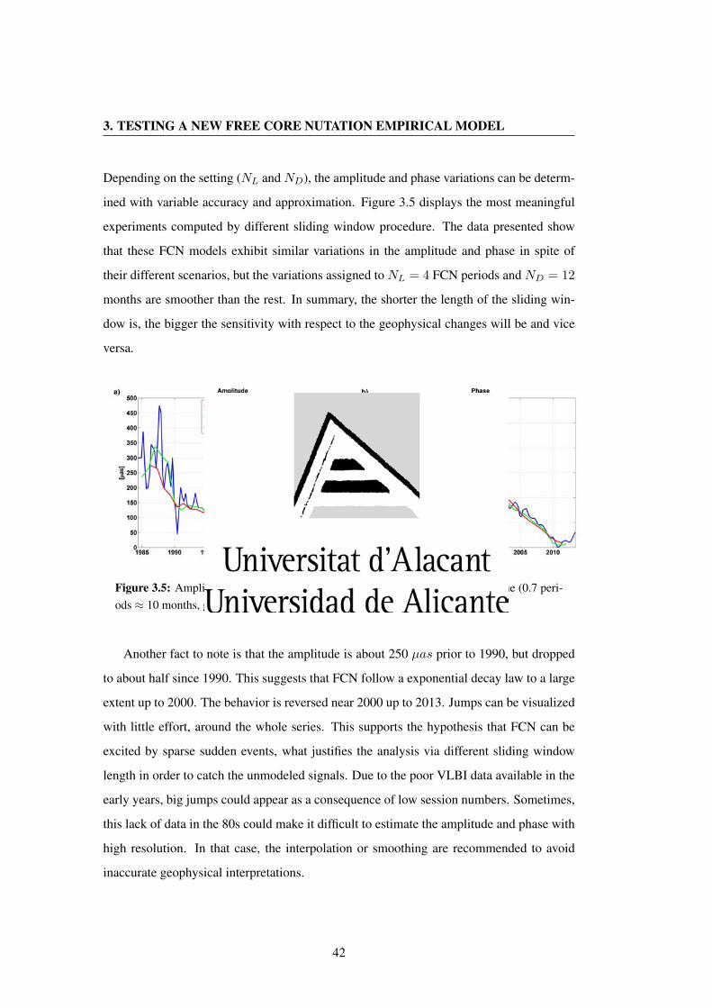
3. TESTING A NEW FREE CORE NUTATION EMPIRICAL MODEL
Depending on the setting (NL and ND), the amplitude and phase variations can be determ-
ined with variable accuracy and approximation. Figure 3.5 displays the most meaningful
experiments computed by different sliding window procedure. The data presented show
that these FCN models exhibit similar variations in the amplitude and phase in spite of
their different scenarios, but the variations assigned to NL = 4 FCN periods and ND = 12
months are smoother than the rest. In summary, the shorter the length of the sliding win-
dow is, the bigger the sensitivity with respect to the geophysical changes will be and vice
versa.
Figure 3.5: Amplitude and phase variations from three different FCN models (blue (0.7 peri-ods ≈ 10 months, green ≈ 2 years, and red ≈ 4.6 years).
Another fact to note is that the amplitude is about 250 µas prior to 1990, but dropped
to about half since 1990. This suggests that FCN follow a exponential decay law to a large
extent up to 2000. The behavior is reversed near 2000 up to 2013. Jumps can be visualized
with little effort, around the whole series. This supports the hypothesis that FCN can be
excited by sparse sudden events, what justifies the analysis via different sliding window
length in order to catch the unmodeled signals. Due to the poor VLBI data available in the
early years, big jumps could appear as a consequence of low session numbers. Sometimes,
this lack of data in the 80s could make it difficult to estimate the amplitude and phase with
high resolution. In that case, the interpolation or smoothing are recommended to avoid
inaccurate geophysical interpretations.
42

3.4 Results
3.4.3 Comparison with other models
Krasna et al. [2013] recently determined a FCN model using groups of 4 years (≈ 3.4 FCN
periods) measurements data displaced one year. Data from 1984.0 to 1988.0 in the first
run were involved and thus the estimates are valid for 1986.0. The second global solution
includes data from 1985.0 till 1989.0 and so on. She used a period of -431.18 sidereal
days. Lambert [2007] estimated a FCN model (IERS Conventions 2010) using a period of
431.39 sidereal days, a sliding window size of two years (730 days≈ 1.7 FCN periods) and
displaced by one year. These models were compared with respect to the different empirical
simulations computed in the previous sections with the aid of the WRMS of the residuals
after removing FCN (figure 3.6).
Figure 3.6: WRMS difference of the residuals between our estimates and Lambert’s (lower)or Krasna (upper) model. FCN effect removed. Right: USNO Finals. Left: IERS 08 C04.White color: no data. Units: µas.
43

3. TESTING A NEW FREE CORE NUTATION EMPIRICAL MODEL
Consequently, in the comparison procedure we expect the minimum WRMS differences
located close to 1.7 and 3.4 FCN cycles, being consistent with the groups of data which
were used for Lambert and Krasna, respectively. That is why a area of low residuals can
be detected in the figure centers, coinciding with the aforementioned cycles (figure 3.6). A
same pattern can be seen with different a priori EOP.
The smallest residuals in the comparison, of about 12 µas, correspond to the Krasna’s
model, along with the USNO Finals as a priori ERP. Lambert’s model achieves errors 10
µas larger than the Krasna model. Note that the best concordance with Krasna model could
be due to the use of the same FCN period and VLBI software (VieVS). Again, the USNO
Finals series as a priori reaches better accuracy than IERS 08 C04. The improvement is
around 2 µas.
3.5 Discussions and Conclusions
Previous studies of FCN mostly focused on FCN’s resonance effect on neighboring astro-
nomical nutations found in VLBI and gravity data. Such indirect evidences are well suited
for estimating FCN’s natural period, but unable to provide information about the behavior
of FCN over time. Direct evidences for the latter begin to emerge as VLBI data quality
improves. In this study, we estimate different empirical FCN models using the residual
VLBI nutation time series from 1984.0 to 2013.0 obtained after the astronomical nutations
are accounted for and then removed according to the IAU 2006/2000A precession model.
Phase and amplitude variations are examined. Furthermore, different EOP (IERS 08 C04
and Usno Finals) are analyzed with a view to know which series achieves the optimal FCN
model. Finally, a comparison with Krasna and Lambert model was done. In all the estim-
ates the period was fixed to the recent value determined by Krasna et al. [2013].
Large number of FCN models were estimated and assessed. The methodology and
the choice of the sliding window length vary for each simulation. Least-squares estimates
of the amplitude were done at each interval of sliding window, where the displacement
between the subsequent fit changes among 1 and 12 months. This investigation confirms
that the use of FCN models determined from the shortest sliding window size substantially
improved the accuracy of the modeling, achieving an improvement in WRMS up to 15
µas. Moreover, the usage of IERS 04 C08 as a priori ERP series gives slightly larger
residuals. Therefore the USNO Finals series provide the better accuracy when assessed
44

3.5 Discussions and Conclusions
with these empirical FCN models. The highest agreement for all our simulations with
different available FCN models occurs close to the corresponding FCN number of cycles:
Krasna’s (3.4 cycles) and Lambert’s (1.7 cycles), with Krasna et al. [2013] being the most
favorable. Our models computed with reduced window lengths show an improvement of
20 µas w.r.t. both, Krasna’s and Lambert’s models. Residuals drop if VLBI sessions from
1984-1990 were eliminated due to the low temporal resolution and accuracy.
The FCN is essentially the only signal that remains above the noise level. It clearly has
a time-variable amplitude during the studied period, as can be demonstrated by a simple
wavelet time-frequency spectrum. A sliding window least-squares fit of the FCN amplitude
yields similar results: To first order, the amplitude hovers around 0.3 mas prior to 1990,
then it drops to about half of that value. Dynamically the FCN is a free-oscillation mode in
the Earth’s rotation and hence a decaying harmonic function of time if left unexcited. Thus
the time-variable amplitude is a clear evidence that the FCN has been subjected to episodic,
if not continual excitations by some geophysical processes. The situation is analogous to
the continual geophysical excitation of the Chandler wobble, another free oscillation in the
Earth’s rotation, resulting in its time-variable amplitude that has been long observed and
studied since around 1900. While the excitation of the Chandler wobble can be traced to
meteorological origin [Furuya et al., 1996; Gross, 2000], long-term variation of the Chand-
ler wobble amplitude has not been explained. Similarly, there has been no clear evidence
as to the excitation source(s) of FCN. In spite of this, the new tested empirical FCN models
of high temporal resolution can help to enhance the understanding about the amplitude and
phase variations, which in turn is related to the geophysical excitations. Wider window
lengths produce smoother amplitude and phase variations and vice versa.
An ultimate pursuit in front of us is to identify the geophysical phenomena that excited
the FCN in the way that is observed. One possible candidate is again meteorological dis-
turbances in the form of broad-band variations of atmospheric, oceanic, and hydrological
angular momentum. Furthermore, on excitation-domain study, one can confidently pre-
sume that some major FCN excitation occurred around 1990. One can further speculate the
possibility of certain large and deep seismic events, some episodic jerky disturbances in the
core, or even major solar mass-ejection events exerting magnetic torques on the Earth.
45

The logic of validation allows us tomove between the two limits of dog-matism and skepticism.
Paul Ricoeur
CHAPTER
4On the decorrelation filtering
of RL05 GRACE data forglobal applications
4.1 Introduction
The GRACE mission was launched in March 17, 2002. The GRACE mission measures the
distance between two twin satellites in near polar orbit. These distances are used to estimate
monthly geopotential spherical harmonics SC, called Level 02 GRACE data, by Center for
Space Research (CSR), GFZ, and Jet Propulsion Laboratory (JPL). Actually, these SC
represent the geopotential differences with respect to a geopotential background, where
some known geophysical processes are modeled: solid Earth and oceanic tides (including
pole tides), non-tidal variability of the atmosphere and ocean, and gravity perturbations due
to the Sun, Moon and the rest of the planets [Bettadpur, 2012; Dahle et al., 2013; Watkins
and Yuan, 2012].
Assuming that the geopotential variations are produced by mass changes at the surface
of the Earth, it is possible to estimate the associated mass maps in form of millimetres
of water thickness equivalent [WTE; Chao, 2005; Wahr et al., 1998]. These maps show
north−south stripes due to some noise in the high degree and order SC. So, they must
47

4. ON THE DECORRELATION FILTERING OF RL05 GRACE DATA
be filtered to reduce that noise. However, there is not a standard filtering procedure and
the GRACE users must decide which is the most convenient in their studies. There are
several ways of filtering the data that can be found in the literature [Duan et al., 2009, and
references therein]. However, one of the most popular filtering procedures, due to its easy
implementation, is a two-step filter that first applies the decorrelation error filter [Swenson
and Wahr, 2006], and then the isotropic Gauss filter [Jekeli, 1981; Swenson and Wahr,
2002]. The decorrelation filter has to be tuned for some parameters, which are left to the
user’s choice. Several authors have used different parameters depending on the application
of the GRACE data [Chambers, 2006; Chambers and Bonin, 2012; Chen et al., 2007; Duan
et al., 2009]. Despite the popularity of the Gaussian filter, the filtering process can be
improved replacing it by an anisotropic filter that fits better the noise of the data [Chen
et al., 2006; Garcıa-Garcıa et al., 2010; Zhang et al., 2009].
From time to time, the procedure to estimate the SC is improved and new sets of SC
are released by the different agencies. In autumn 2012, a new release of GRACE data was
published, called RL05. This new release presents less noise than previous releases due to
the improvement in the knowledge of alignments between the star camera, accelerometer,
and K-band ranging system for Level-1B data, and updated mean gravity field, ocean tide,
pole tide and de-aliasing models for Level-2 processing. Therefore, the parameters of the
decorrelation filter must be tuned again. Chambers and Bonin [2012] optimized those
parameters for ocean applications of the RL05 of GRACE data. In this study the choice
of optimal parameters is explored for global applications of the same data set, extending
the work that Duan et al. [2009] did for the RL04 GRACE data. The two-step filter is also
analysed. The optimal radius of the Gauss filter is studied, as well as the application of an
alternative anisotropic filter [Zhang et al., 2009].
4.2 Data description and methodology
The level 02 RL05 GRACE data from CSR, GFZ and JPL are used in this study1. Data
consists of monthly sets of SC spanning from 2004/01 to 2011/12 (except GFZ that starts
in 2004/02), with missing values in 2011/01, and 2011/06. During the last months, some
components of the GRACE satellites were disconnected in order to minimize the battery
problems, and to extend the life of the mission as much as possible. The C20 coefficient is
1http://podaac.jpl.nasa.gov/gravity/grace
48

4.2 Data description and methodology
usually replaced by an estimate from Satellite Laser Ranging [Cheng and Ries, 2007]; it is
excluded from the analysis. As far as we are interested in the variability of the geopotential,
the mean value of the whole period is subtracted.
Assuming that the gravity variations are produced by mass variations on the surface
of the Earth (such as the water mass transport within the water cycle, the biggest mass
variations of the Earth in the intra-annual timescale), the surface mass variation, σ, in terms
of water thickness equivalent (WTE) can be uniquely determined as:
σ(θ, λ, t) =aρE
3
∞∑l=0
l∑m=0
(2l + 1)
1 + k′lPlm cos(θ)[Clm(t) cos(mλ)+Slm(t) sin(mλ)] (4.1)
[Chao, 2005; Wahr et al., 1998], where (θ, λ, t) = (colatitude, longitude, time), a and ρEare the equatorial radius and the mean density of the Earth, k′l is the degree-l load Love
number, Plm is the 4π-normalized associated Legendre function of degree l and order m
and Clm(t) and Slm(t) are the monthly GRACE SC.
Swenson and Wahr [2006] found, for a fixed order, a correlated error for the SC of even
and odd degrees. They proposed a decorrelation filter that, for any SC of even (odd) degree,
removes a polynomial fitted to some of the adjacent SC of even (odd) degree, which define
a moving window. However, the degree of the polynomial or the length of the window
was not specified and must be selected by the users. Besides, a portion of low degree and
order SC is usually unfiltered, which must also be chosen by the users. An analysis of
several configurations of the filter can be found in Duan et al. [2009], as those made (but
not published) by Swenson and Wahr [2006], by Chambers [2006] for ocean applications
and by Chen et al. [2007] to study the 2004 Sumatra earthquake.
Duan et al. [2009] presented a configuration of the filter similar to Swenson and Wahr
[2006]. The idea is filtering stronger where the noise is higher, which can be achieved by
increasing the order of the fitting polynomial or reducing the length of the window as the
noise increase. They fixed the polynomial degree to 2 and vary the length of the window,
ω, accordingly to,
ω = max
{Ae−
[(1−γ)mp+γlp]1p
k + 1, 5
}(4.2)
where l and m are the degree and order, respectively, of the SC to be filtered, which is
located in the center of that window; andA, k, γ and p are the parameters to be fixed, which
49

4. ON THE DECORRELATION FILTERING OF RL05 GRACE DATA
define the filter itself. Fig. 4.1 shows, for each degree and order, the length of the associated
window accordingly to eq. 4.2 for a selection of parameters. They are clustered in bands,
where number, width, slope and curvature are defined by A, k, γ and p, respectively. The
width of the window decreases (increases) as A or k decreases (increases), which would
make the filter stronger (weaker).
The minimum length of the window is fixed to 5 to retain some information after sub-
tracting the polynomial of degree 2. In order to keep the SC to be filtered in the center of
the window, the length of the latter is rounded to the nearest odd number. So, the polyno-
mial of degree 2 to be subtracted from the SC of degree l and order m, Clm and Slm, will
be fitted to, Cl−2α,m, ... , Cl−2,m, Cl,m, Cl+2,m, ... , Cl+2α,m , and Sl−2α,m, ... , Sl−2,m,
Sl,m, Sl+2,m, ... , Sl+2α,m, respectively, where ω = 2α+ 1. Only in the case that l is close
to the maximum degree available in the data, or to the order m, the window is not centered
in Clm and Slm.
Note that the decorrelation filter has been applied in a different way by Chambers
[2006], Chambers and Bonin [2012] and Chen et al. [2007], who, for a fixed order, fit-
ted and subtracted a single polynomial for all the SC of even or odd degree.
The low degree and order SC are less noisy, and for that reason are not usually filtered
by the decorrelation filter. Based in a trial and error procedure, Chambers [2006] left
unfiltered the SC with degree and order lower than 7 for RL02 GRACE data, and lower than
11 for RL04 GRACE data1. Chen et al. [2007] left unfiltered the SC of degree and order
below 5 for RL04 GRACE data. On the other hand, Duan et al. [2009] chose the unfiltered
SC based in the calibrated SD provided by the agencies of the RL04 GRACE of one single
month (as all the months look similar). They fit a curve to a SD value close to 1 (×1012)
and left unfiltered the SC below that curve. For RL05 GRACE it is expected that the SD
decrease with respect to former releases, and then the unfiltered portion of SC should be
increased. For example, Chambers and Bonin [2012] showed that leaving unfiltered the
SC with degree and order lower than 15 improves the statistics when comparing GRACE
with ocean models. We will explore the influence of the unfiltered SC including an extra
parameter, l, in the filter. Then, for each degree l we define a curve going from (degree,
order) = (l, 0) to (degree, order) = (m,m) that fits the SD in fig. 4.2. For example, for
l = 38 the value of m is 11. Then, we left unfiltered the SC below that curve. In RL05, the
calibrated SD are only available for GFZ GRACE data.
1http://grace.jpl.nasa.gov/files/GRACE-dpc200711RL04.pdf
50

4.2 Data description and methodology
Figure 4.1: Length of the window accordingly to eq. 4.2 for each degree and order, and fordifferent parameters configurations: (a) A = 14, k = 44, γ = 0.04, p = 1; (b) A = 14,
k = 44, γ = 0.5, p = 1; (c) A = 14, k = 44, γ = 0.04, p = 3.4; (d) A = 14, k = 10,
γ = 0.04, p = 3.4; (e) A = 14, k = 24, γ = 0.04, p = 3.4; (f) A = 21, k = 24, γ = 0.04,
p = 3.4.
51

4. ON THE DECORRELATION FILTERING OF RL05 GRACE DATA
We use the time average for the whole period of the formal (not calibrated) SD of the SC
from GFZ and JPL data (they are not available for CSR data). Fig. 4.2 shows the SD of the
JPL GRACE data, which is similar to those from GFZ, and it is expected to be similar to
those from CSR, as far as it was in previous releases.
Figure 4.2: Time average of the formal (not calibrated) SD (scaled by×1012) of the JPL RL05GRACE SC. Black lines represent the curves delimiting the unfiltered SC for l = 28, 38 and43.
The width of the moving window must vary accordingly to the noise of the data. So,
the color bands shown in fig. 4.1 should be aligned with those in fig. 4.2. Following that
criteria it is easy to fix the parameters γ = 0.04 and p = 3.4. Then, the filter will be defined
once the values ofA, k and l are determined. We implement several experiments for a wide
rank of parameters in order to define an optimal filter for global applications. In particular,
GRACE and synthetic GRACE data (see below) are filtered with parameters: A from 10 to
24; k from 20 to 44 and l from 10 to 45. In order to reduce the high computational cost of
the experiments, the parameters A and k vary 2 by 2, and l does 5 by 5 from 10 to 30, and
1 by 1 from 30 to 45.
For the following experiments we will need synthetic GRACE data, which consist of
global grids with OBP over the oceans and with terrestrial water storage fields over land.
The former is estimated from the Estimating the Circulation and Climate of the Ocean
52

4.3 First-Step Filter
(ECCO) [Stammer et al., 2002]1 model version kf080, and the latter is estimated from
surface water storage grids from Global Land Data Assimilation Systems (GLDAS) model
[Rodell et al., 2004]2. These grids are estimated from the integration of four-layer soil
moisture, snow equivalent height and canopy water. As the hydrologic model has no data
over Greenland and Antarctica, these regions are avoided in the comparison with GRACE.
In order to make the synthetic data more realistic an estimate of the Post Glacial Rebound
(PGR) from Paulson et al. [2007] have been added to the grids. The synthetic data have
been reduced to 1◦× 1◦ monthly grids for the period 2004/01 to 2011/12, and transformed
to millimetre of WTE (kg ·m2). The mean value of the whole period is removed from the
signal. The points covered neither by GLDAS nor ECCO are set to zero. When the filter is
applied to the synthetic data, the degree-1 and the C20 coefficients are set to zero.
4.3 First-Step Filter
4.3.1 Linear trends
When filtering the data, the noise is reduced jointly with some of the sought geophysical
signals. On the one hand, if the filter is very weak the noise will dominate the signal. On
the other hand, if the filter is very strong the geophysical signal will be too attenuated. In
some place between these two opposite cases resides the optimal filtering level. In order to
find the latter, we explore the strategy used by Duan et al. [2009] to select the parameters
of the filter for RL04 GRACE data, who found the values A = 30, k = 15, γ = 0.1, p = 2
for CSR data and A = 30, k = 15, γ = 0.1, p = 3 for JPL data.
The selection is based on the study of the rms of the lineal trend of surface mass grids
from GRACE and synthetic data. The unfiltered GRACE data present too high linear trend
values, with an associated high rms, due to noise influence. So, the reduction of such
trends (and associated rms) would indicate a reduction of the noise. However, an excessive
reduction would mean an undesirable attenuation of the geophysical signals. In order to
estimate the latter, the filter is applied to noise-free data based on models, the synthetic
data. The perfect filter should not reduce the trends of noise-free data. The optimal filter
should minimize the rms of the global linear trend in GRACE data, and maximize them in
synthetic data. In practice, the rms of the filtered GRACE and synthetic data are normalized
1http://www.ecco-group.org/products.htm2http://disc.sci.gsfc.nasa.gov/hydrology/data-holdings
53

4. ON THE DECORRELATION FILTERING OF RL05 GRACE DATA
with respect to their rms prior to filtering. This is made to reduce the influence of the high
values produced by very noisy GRACE data. After normalization, the linear trend rms
from synthetic data present higher values than those from GRACE data. It makes sense
since the filter produces attenuation of the signal in both data, but noise reduction only in
GRACE data. Therefore, the optimal filter should maximize the difference between the
linear trends rms of synthetic and GRACE data. Fig. 4.3 shows the latitude weighted rms
of the linear trends for synthetic, and the three agencies GRACE data, and fig. 4.4 shows
their differences.
Figure 4.3: The rms of the linear trends from (a) synthetic, and GRACE data: (b) CSR; (c) JPLand (d) GFZ. Each value is estimated using a decorrelation filter with different combination ofA (from 10 to 24, 2 by 2), k (from 20 to 44, 2 by 2) and l (5 by 5 from 10 to 30, and 1 by 1
from 30 to 45). Units: Percentage with respect to rms prior filtering.
54

4.3 First-Step Filter
Each value is estimated using a different combination of A, k and l. The parameter l
shows de greatest gradient, with optimal values between 35 and 45, and several combin-
ations of A and k. For example, for CSR and l = 38, the greatest differences can be
reached around (A, k) = (24, 20). This experiment gives an idea about the importance of
the parameter l, and justifies the finer resolution between 30 and 45. However, the choice
of the parameters is too vague and further analyses are needed.
Figure 4.4: Differences between the rms of the linear trends from synthetic and GRACE data:(a) CSR, (b) GFZ and (c) JPL. Decorrelation filter applied to GRACE and synthetic data priorsubtraction. Units: Percentage with respect to rms prior filtering.
55

4. ON THE DECORRELATION FILTERING OF RL05 GRACE DATA
4.3.2 GRACE versus synthetic data
GRACE and synthetic data are compared, but some preliminary corrections must be made
to the GRACE data. First, as synthetic data represent OBP over the ocean, GRACE should
represent the same. It is reached in two steps: (1) the atmospheric and oceanic correc-
tions applied to GRACE over the ocean, the GAD product, is added back and (2) for each
month the global ocean Sea Level Pressure (SLP) (from NCEP) average is subtracted from
the ocean points in GRACE. Note that the GAD and SLP data are not filtered, so they
may modify the absolute values of the linear trends experiment, but not the relative values
among them, which we were interested in the previous experiment. Secondly, to make the
spatial resolution comparable the synthetic grids are transformed into SC, and then back
to grids only using SC up to degree 60. In the processes the degree-1 and C20 coefficients
are suppressed. No filter is applied. Finally, the regions not covered by the synthetic data-
Antarctica, Greenland and Artic ocean-are discarded in the analysis, and the continental
leakage is reduced [Wahr et al., 1998].
Since the decorrelation filtered GRACE data are still too noisy to be compared to the
unfiltered synthetic data, a Gaussian filter of 500 km radius is also applied to the former.
The Gaussian filter is defined by a radius r, and consists of the application of a weight,W rl ,
to the SC [see Swenson and Wahr, 2002, for a recursive formula]. Then, the surface mass
grids are estimated as
σ(θ, λ, t) =aρE
3
∞∑l=0
l∑m=0
(2l + 1)
1 + k′l
×W rl Plm cos(θ)[C∗lm(t) cos(mλ) + S∗lm(t) sin(mλ)] (4.3)
where C∗lm(t) and S∗lm(t) are the SC once the decorrelation filter has been applied. Note
that the only other difference with eq. 4.1 is the term W rl .
For each gridpoint the rms of the difference between filtered GRACE and unfiltered
synthetic data is estimated. Fig. 4.5 shows the spatial average of these rms for different
parameters of the filter. The minimum values are reached with parameters 36 ≤ l ≤ 39,
10 ≤ A ≤ 16 and 20 ≤ k ≤ 28. Similarly, the correlation coefficient between filtered
GRACE and unfiltered synthetic data is shown in fig. 4.6. The maximum correlations are
reached with 38 ≤ l ≤ 39, A ∼ 14 and 20 ≤ k ≤ 28 for CSR data, and with 36 ≤ l ≤ 40,
10 ≤ A ≤ 14 and 20 ≤ k ≤ 28 for GFZ and JPL data. Therefore, for all GRACE
56

4.3 First-Step Filter
data sets the minimum residual and the maximum correlation is reached around the same
parameters, narrowing the parameters values selected by the linear trends experiment.
Figure 4.5: The rms of the differences between synthetic and GRACE data: (a) CSR, (b) GFZand (c) JPL. Decorrelation and Gauss (r = 500 km) filter applied to GRACE data. Syntheticdata truncated at degree 60. Continental leakage reduced. Units: mm.
It is worthwhile to remark that the minimum difference between GRACE and synthetic
do not necessary define the optimal filter. The reason is that GRACE measures signals
that hydrological models generally do not account for, as for example groundwater, river
storage or water extraction from aquifers. Besides, during the filtering process the signal
amplitude is attenuated and it must be restored to approximate the real signal,which can be
done for regional averaged signals [e.g. Velicogna and Wahr, 2006] or gridpoints [Landerer
and Swenson, 2012]. In the restoring amplitude process the differences with the synthetic
data are not necessarily reduced. On the other hand, the correlation coefficient does not
57

4. ON THE DECORRELATION FILTERING OF RL05 GRACE DATA
depends on whether the amplitude of a time-series is restored, since the restoring factor is
a constant multiplying the whole time-series.
Figure 4.6: Correlation coefficients between synthetic and GRACE data: (a) CSR, (b) GFZand (c) JPL. Data processing as in fig. 4.5.
The annual amplitude has been estimated for each gridpoint of GRACE and synthetic
data. Fig. 4.7 shows the correlation coefficients between them. The maximum correlation
is reached for the greatest values of A, k and l, that is, for the weakest version of the
filter. It makes sense since the estimation of the annual amplitudes acts as a filter itself. On
the other hand, fig. 4.8 shows that a stronger version of the filter with lower l is needed
to reach the maximum correlation of the non-seasonal signals (no linear trend nor annual
amplitude). It means that a modification of the parameters must be considered depending
on the sought-after signal.
58

4.3 First-Step Filter
Figure 4.7: Correlation coefficients between the annual amplitudes of synthetic and GRACEdata: (a) CSR, (b) GFZ and (c) JPL. Data processing as in fig. 4.5.
4.3.3 Contienents versus ocean
The optimal filter can also be explored using the criteria that Chen et al. [2007] defined for
tuning their anisotropic filter. The idea is based on the fact that the surface mass variability
is stronger in the continents than in the oceans. The ratio of variability can be measured as
the quotient of the latitude weighted rms of the continental and oceanic signals. On the one
hand, if some noise were added to the SC, spurious variability would be introduced in both
continents and oceans. On the other hand, if the SC were attenuated the variability in both
continents and oceans would be reduced. In any case, the ratio of variability between the
continents and the ocean would be reduced. So, the maximum of such ratio would represent
the maximum of signal-to-noise ratio,which should be obtained using the optimal filter.
59
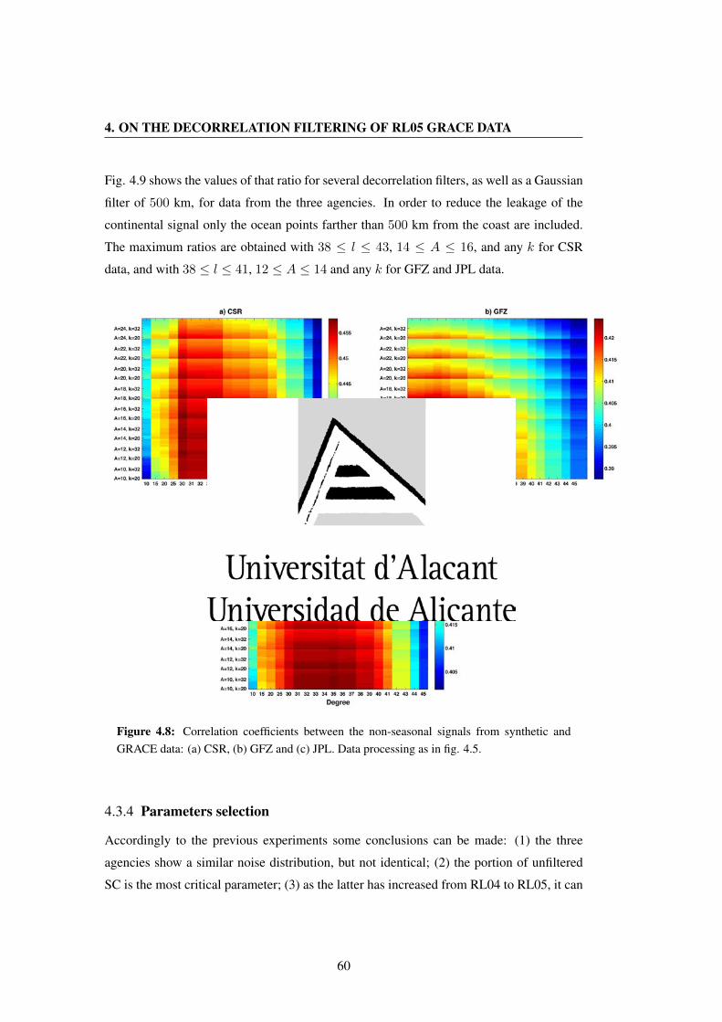
4. ON THE DECORRELATION FILTERING OF RL05 GRACE DATA
Fig. 4.9 shows the values of that ratio for several decorrelation filters, as well as a Gaussian
filter of 500 km, for data from the three agencies. In order to reduce the leakage of the
continental signal only the ocean points farther than 500 km from the coast are included.
The maximum ratios are obtained with 38 ≤ l ≤ 43, 14 ≤ A ≤ 16, and any k for CSR
data, and with 38 ≤ l ≤ 41, 12 ≤ A ≤ 14 and any k for GFZ and JPL data.
Figure 4.8: Correlation coefficients between the non-seasonal signals from synthetic andGRACE data: (a) CSR, (b) GFZ and (c) JPL. Data processing as in fig. 4.5.
4.3.4 Parameters selection
Accordingly to the previous experiments some conclusions can be made: (1) the three
agencies show a similar noise distribution, but not identical; (2) the portion of unfiltered
SC is the most critical parameter; (3) as the latter has increased from RL04 to RL05, it can
60

4.3 First-Step Filter
be inferred that RL05 data are less noisy than RL04 and (4) the optimal statistics of the
experiments is not reached for a unique parameters configuration, but for all the agencies
it can be reached with parameters values close to l = 38, A = 14 and k = 24. In Sections
4.3.2 and 4.3.3, a Gaussian filter with a radius of 500 km was also applied to GRACE data.
In order to check whether that choice could vary the optimal parameters of the decorrelation
filter, the same analysis was implemented with a radius of 300 km. In that case, the obtained
results were quite similar.
Figure 4.9: Ratio of variability between the continents and the ocean: (a) CSR, (b) GFZ and(c) JPL. Decorrelation and Gauss (r = 500 km) filter applied to GRACE data. Ocean pointscloser to 500 km to the continents are avoided.
61
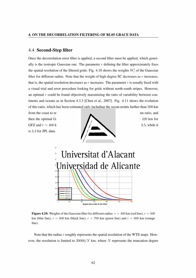
4. ON THE DECORRELATION FILTERING OF RL05 GRACE DATA
4.4 Second-Step filter
Once the decorrelation error filter is applied, a second filter must be applied, which gener-
ally is the isotropic Gaussian one. The parameter r defining the filter approximately fixes
the spatial resolution of the filtered grids. Fig. 4.10 shows the weights W lr of the Gaussian
filter for different radius. Note that the weight of high degree SC decreases as r increases,
that is, the spatial resolution decreases as r increases. The parameter r is usually fixed with
a visual trial and error procedure looking for grids without north-south stripes. However,
an optimal r could be found objectively maximizing the ratio of variability between con-
tinents and oceans as in Section 4.3.3 [Chen et al., 2007]. Fig. 4.11 shows the evolution
of this ratio, which has been estimated only including the ocean points farther than 500 km
from the coast to reduce the leakage from the continental signal. The maximum ratio, and
then the optimal Gaussian filter, is obtained with r = 380 km for CSR, r = 420 km for
GFZ and r = 400 km for JPL. The maximum ratio in CSR and GFZ data is ∼ 3.5, while it
is 3.3 for JPL data.
Figure 4.10: Weights of the Gaussian filter for different radius: r = 400 km (red line), r = 500
km (blue line), r = 600 km (black line), r = 700 km (green line) and r = 800 km (orangeline).
Note that the radius r roughly represents the spatial resolution of the WTE maps. How-
ever, the resolution is limited to 20000/N km, where N represents the truncation degree
62

4.4 Second-Step filter
of the SC. So, if N = 40 and N = 60 a maximum spatial resolution of 500 and ∼ 333 km
could be reached, respectively. For that reason, the reported values of r must be interpreted
carefully.
In order to estimate the error of the data, the residuals of the differences between
GRACE and synthetic data are explored as in Section 4.3.2, but using the optimal r of each
agency. Then, the standard deviation of the residual is estimated for each gridpoint. Fig.
4.12 shows the residual for the CSR, GFZ and JPL data using SC up to degree 60,which are
very similar. The global latitude-weighted averaged of the residuals are 26.1 mm for CSR
and GFZ, and 26.5 mm for JPL. The largest signal is observed around Greenland,which is
not modeled by the hydrological model, and in the Amazon, where the surface waters are
neither modeled. When these two regions are avoided the residuals are reduced to 24.6 mm
for CSR and GFZ and 25.0 mm for JPL. Besides, when the continental leakage is reduced,
the residual drops around 1.5 per cent. In any case, remember that noise-free GRACE data
are not expected to minimize the residual.
Figure 4.11: Ratio of variability between continents and ocean for GRACE data from: (a)CSR, (b) JPL and (c) GFZ, as a function of the radius r of the Gaussian filter. GRACE datahave been previously decorrelated. Ocean points closer to 500 km to the continents are avoided.
The two-step filtering process can be improved replacing the isotropic (only degree
dependent) Gauss filter by an anisotropic (degree and order dependent) filter. The Gaussian
filter applies weights to the SC that decreases as the degree increases. The fan filter is a
combination of two Gaussian filters, one applied to the degrees, and another to the orders
63

4. ON THE DECORRELATION FILTERING OF RL05 GRACE DATA
[Zhang et al., 2009]. Then, the fan filter can be defined with two radii, one for the degrees,
rl, and another for the orders, rm. In this case, the surface mass grids are estimated as
σ(θ, λ, t) =aρE
3
∞∑l=0
l∑m=0
(2l + 1)
1 + k′l
×W rll W
rmm Plm cos(θ)[C∗lm(t) cos(mλ) + S∗lm(t) sin(mλ)] (4.4)
where the weights W rll and W rm
m depends on the degree l and order m, respectively. Note
that the only difference with eq. 4.3 is the term W rmm .
Figure 4.12: Standard deviation of the residual between synthetic and filtered GRACE data:(a) CSR, (b) JPL and (c) GFZ. Decorrelation and Gauss (r = 380 km for CSR, r = 420 kmfor GFZ and r = 400 km for JPL) filter applied to GRACE data. Synthetic data truncated atdegree 60. Continental leakage reduced.
In the Gauss filter the radio r roughly represents the spatial resolution in any direction,
while rl and√
2·rm represent the north-south and east-west spatial resolution, respectively.
64

4.5 Discussion
Similarly to the Gauss filter, the optimal radii of the fan filter are explored to maximize the
ratios of variability between continents and oceans. Fig. 4.13 shows that the largest ratios
are reached with radii close to (rl, rm) = (290, 690) km for CSR, (rl, rm) = (310, 820)
km for GFZ and (rl, rm) = (290, 640) km for JPL. The obtained ratios are larger with
the fan filter than with the Gauss filter. Although, the residuals of the differences between
GRACE and synthetic data look similar (not shown), their average is 25.4 mm for CSR,
25.3 mm for GFZ and 26.1 mm for JPL. When the points from Amazon and around Green-
land are excluded, the residuals are reduced to 23.9 mm for CSR and GFZ and 24.6 mm for
JPL. In any case, the residuals are smaller than using the Gauss filter. Then, the fan filter
seems to be more appropriated than the Gauss filter as second-step filter.
4.5 Discussion
GRACE data must be filtered before use to reduce some noise in high degree and order SC.
One of the most popular filters is a two-step filter: (1) decorrelation filter and (2) Gauss
filter. Both filters must be adapted to the noise level of the data. While the Gauss filter only
depends on one parameter, the decorrelation filter depends on several parameters produ-
cing multiple combinations. In this study we have analyzed the parameters configurations
of the decorrelation filter for the RL05 of GRACE data that optimize several statistics for
global applications. These parameters are close to l = 38, A = 14 and k = 24, as well as
γ = 0.04 and p = 3.4, for all the agencies. Besides, the application of the isotropic
Gauss filter and the anisotropic fan filter as second-step filter has been analysed. The best
results for the Gauss filter are obtained with r = 380 km for CSR, r = 420 km for
GFZ and r = 400 km for JPL, while for the fan filter are obtained with values close to
(rl, rm) = (290, 690) km for CSR, (rl, rm) = (310, 820) km for GFZ and
(rl, rm) = (290, 640) km for JPL.
Table 4.1 summarizes the analysed statistics of the reported filters, as well as those
using parameter configuration from previous studies. In order to make the different filters
comparable, the calculation are made using SC up to degree 40 as in Chambers and Bonin
[2012], and up to degree 60 as in Duan et al. [2009] and Chen et al. [2007]. In both
cases, and for any agency, the parameters estimated in this study show: (1) smaller rms
values in the linear trends of GRACE data; (2) smaller differences and larger correlation
with the synthetic data; (3) larger variability ratios between continents and ocean signals,
65
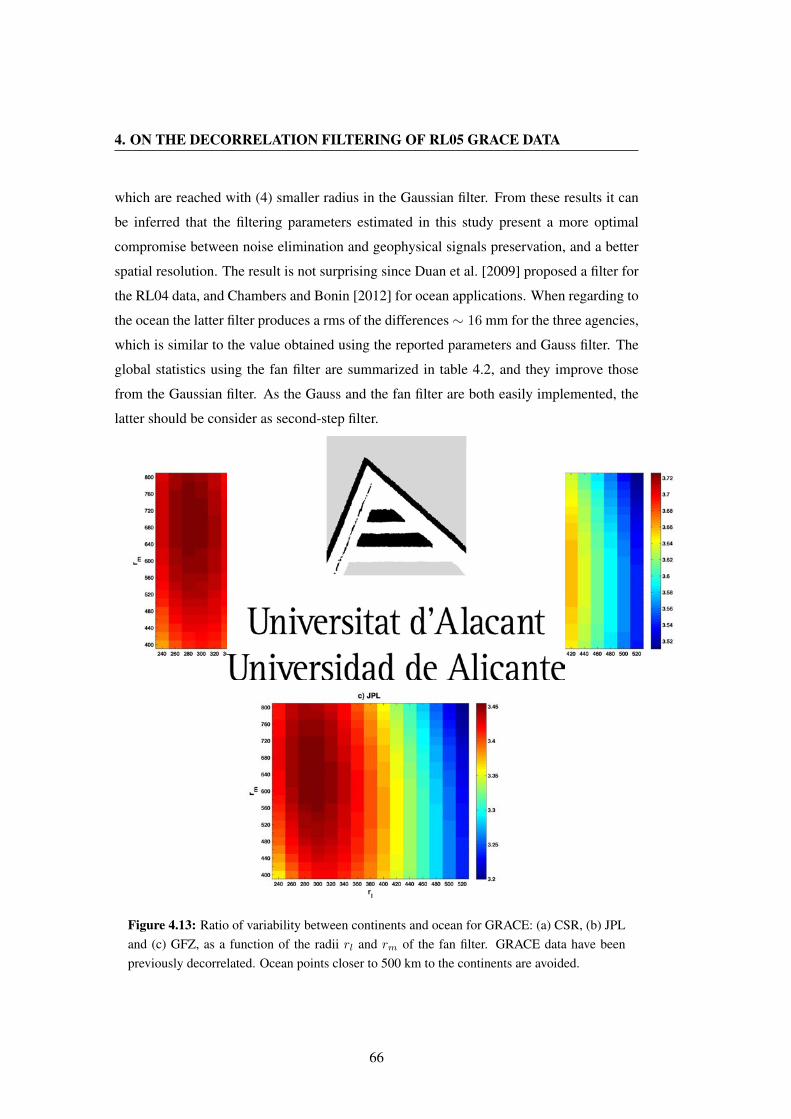
4. ON THE DECORRELATION FILTERING OF RL05 GRACE DATA
which are reached with (4) smaller radius in the Gaussian filter. From these results it can
be inferred that the filtering parameters estimated in this study present a more optimal
compromise between noise elimination and geophysical signals preservation, and a better
spatial resolution. The result is not surprising since Duan et al. [2009] proposed a filter for
the RL04 data, and Chambers and Bonin [2012] for ocean applications. When regarding to
the ocean the latter filter produces a rms of the differences∼ 16 mm for the three agencies,
which is similar to the value obtained using the reported parameters and Gauss filter. The
global statistics using the fan filter are summarized in table 4.2, and they improve those
from the Gaussian filter. As the Gauss and the fan filter are both easily implemented, the
latter should be consider as second-step filter.
Figure 4.13: Ratio of variability between continents and ocean for GRACE: (a) CSR, (b) JPLand (c) GFZ, as a function of the radii rl and rm of the fan filter. GRACE data have beenpreviously decorrelated. Ocean points closer to 500 km to the continents are avoided.
66

4.5 Discussion
The selection of the parameters, and hence the design of the two-step filter depends
on the models used in the synthetic data. However, the study of the variability between
continents and oceans does not depend on the model and gives an approximation of the
filter. Then, the results are not expected to vary significantly as the models change.
This study complements the one done by Chambers and Bonin [2012] for oceanic ap-
plications, and it could be of interest for GRACE users that would like to continue pro-
cessing the RL05 data with the decorrelation filter.
Decorrelation Decorrelation and Gauss filters
Rms linear Rms Correlation Ratio r(km)trend (mm yr−1) differences (mm) coeficients contients/ocean
Degree 60 Chen et al. [2007] CSR 10.7 25.8 0.53 3.27 500GFZ 10.8 25.6 0.52 3.27 600JPL 11.0 26.3 0.52 2.98 540
Duan et al. [2009] CSR 10.8 25.8 0.53 3.32 490GFZ - - - - -JPL 11.5 25.9 0.53 3.03 540
This study CSR 9.7 26.1 0.54 3.53 380GFZ 9.6 26.1 0.52 3.52 420JPL 9.6 26.5 0.53 3.31 400
Degree 40 Chambers and Bonin [2012] CSR 9.2 26.3 0.52 3.35 430GFZ 9.0 25.8 0.52 3.37 520JPL 9.0 26.6 0.52 3.09 480
This study CSR 8.9 26.1 0.53 3.54 380GFZ 8.7 26.1 0.52 3.52 420JPL 8.7 26.4 0.53 3.32 400
Table 4.1: For the three agencies of GRACE data: rms of linear trends from decorrelationfiltered GRACE data. The rms of the differences and correlation coefficients between GRACE(decorrelation and Gauss filters) and synthetic data. Maximum ratio of variability continent-s/oceans from decorrelation and Gauss filtered GRACE data, as well as the radio where themaximum is reached. For comparison purposes the maximum degree is set to 40 and 60.
Decorrelation and fan filters
Rms Correlation Ratio rl/rm (km)differences (mm) coefficients conti./ocean
Degree 60 CSR 25.4 0.55 3.68 290/690GFZ 25.3 0.53 3.73 310/820JPL 26.1 0.54 3.45 290/640
Degree 40 CSR 25.3 0.54 3.70 290/690GFZ 25.3 0.53 3.75 310/820JPL 25.9 0.53 3.48 290/640
Table 4.2: As table 1, but fan filter is used of Gauss filter.
67


Historical methodology, as I see it, is aproduct of common sense applied to cir-cumstances.
Samuel E. Morison
CHAPTER
5A Cautionary Note on theUse of Running Trends as
Summary Statistics forUnivariate Time Series and
Time Series Association
5.1 Introduction
RTA is one of several methods used in climate research to analyze univariate time series
and time series association. For a given time series {y(t)} , observed at n equally spaced
points in time t1, t2, . . . , tn, RTA involves defining n − L + 1 overlapping time windows,
W1,W2, . . . ,Wn−L+1, each with exactly L consecutive time points tj , tj+1, . . . , tj+L−1,
j = 1, 2, . . . , n−L+1, and then evaluating the least square estimates of the trend for each
time window Wj . This produces a new series of length n − L + 1 called running trend
series, that is used as a summary statistic of the original series {y(t)} for further analysis.
In recent years RTA has been widely used in applied research on climate as a part
of more complex time series analysis. Holgate and Woodworth [2004], for example, use
69

5. A CAUTIONARY NOTE ON THE USE OF RUNNING TRENDS
ten-year Global Mean Sea Level (GMSL) running trends (L=10) to study acceleration of
GMSL from 1948 to 2002 and to obtain a GMSL reconstruction for the same period. Santer
et al. [2014] use 120-month running trends (L=120) of changes in the temperature of the
lower troposphere (from satellite measurements made by Microwave Sounding Units on
National Oceanic and Atmospheric Administration polar-orbiting satellites) for the period
1979-2012, to analyze volcanic contributions to observed changes in warming rates.
Hamlington et al. [2014; 2013], use twenty-year running trends of Pacific Decadal
Oscillation (PDO) and of Annual Mean Sean Level to study the contribution of PDO to
Mean Sea level trends both globally [Hamlington et al., 2013] and regionally [Hamlington
et al., 2013]. Palmer and McNeall [2014] compute ten-year running trends of the total
energy in the Earth System (TE), the Global surface temperature (GST) and the total near-
global Ocean heat (OHC), to investigate the relationship between these variables (the model
data analyzed are multi-century pre-industrial control simulations from the Couple Model
Intercomparison Project 5 (CMIP5) model archive). In the same work the authors use
the correlations between running trends in TE and running trends in OHC for a range of
periods (running trends of length 2-36 months are considered) to estimate the time scale
on which the ocean becomes the dominant term in the planetary energy budget. Risbey
et al. [2014] use fifteen-year Global mean surface air temperature (GMST) running trends
evaluated using data from CMIP5 models and observations for the period 1880-2012 to
study the CMIP5 models’ performance (in terms of model’s ability to reproduce the fifteen-
year observed GMST trends).
There is no doubt that RTA might be a useful descriptive tool, but, despite its general
use in applied research, precisely what it reveals about the underlying time series and time
series association is unclear and, as a result, its interpretation is unclear too. In this respect
a more rigorous study of the information that RTA conveys about the underlying time series
and time series association would be desirable. This chapter is intended as a first step in
this direction. We provide an explicit formula for the set of time series that share a given
series of running trends by showing that such a set is the solution set (of dimension L− 1)
of a linear system with n − L + 1 equations and n unknowns. Such a representation
allows us to clarify important aspects of strengths and limitations of running trends as
summary statistics for univariate time series and time series association. The main result
of this chapter, which is the explicit formula for the set of time series with a given series of
running trends, is presented in section 5.2 and illustrated with an example in section 5.3.
70

5.2 Main Result
The worked example also serves to anticipate some important consequences that follows
from the main result in section 5.2 and that we discuss in more general terms in section 5.4.
Concluding remarks and ideas for future work are outlined in section 5.5.
5.2 Main ResultConsider n equally spaced time points t1, t2, . . . , tn, and let ∆ be the common length of
the time interval between two consecutive points in time. We have:
tk = t1 + k∆, k = 0, 1, . . . , n− 1.
Let L be a positive integer such that 2 ≤ L ≤ n − 1 and let W1,W2, . . . ,Wn−L+1 be
overlapping time windows of length L∆ defined starting from t1 and advancing by ∆ at a
time,
Wj = {tj , tj+1, . . . , tj+L−1}, j = 1, 2, . . . , N − L+ 1.
Each time windows Wj contains exactly L of the n time points t1, t2, . . . , tn.
For a generic time series {yt} = (yt1 , yt2 , . . . , ytn) we define the running trend series
associated to {yt} as the series {mj} = (m1, m2, . . . , mn−L+1) of the the least square
estimates of the trend for the time windows Wj . That is mj is the least square estimate of
the slope mj in the linear regression
ytj+h−1= bj +mj · (tj+h−1 − tj) + εtj+h−1
, h = 1, 2, . . . , L, (5.1)
where tj =∑Li=1 tj+i−1
L and εtj+h−1is an error term.
Let m?1,m
?2, . . . ,m
?n−L+1 be n−L+1 arbitrary values. We provide a recursive formula to
obtain the set of all time series {yt} = (yt1 , yt2 , . . . , ytn) for which the corresponding trend
series {mj} = (m1, m2, . . . , mn−L+1) is exactly m?1,m
?2, . . . , m
?n−L+1 and we prove that
such a set is a vector space of dimension L − 1. The details are provided in the following
theorem (for a proof see the appendix A.1).
Main result . Let m?1,m
?2, . . . ,m
?n−L+1 be an arbitrary vector in Rn−L+1.
(i) The set S? of all time series {yt} = (yt1 , yt2 , . . . , ytn) for which the correspond-ing trend series {mj} = (m1, m2, . . . , mn−L+1) is exactlym?
1,m?2, . . . ,m
?n−L+1
is a vector space of dimension L− 1;
(ii) The generic element in S? is a time series (yt1 , yt2 , . . . , ytn), where
71

5. A CAUTIONARY NOTE ON THE USE OF RUNNING TRENDS
• (ytn−L+2 , ytn−L+3 , . . . , ytn) can be arbitrarily chosen in RL−1,
• (yt1 , yt2 , . . . , ytn−L+1) can be found using the recursive relation
ytn−L+1−j =1
t1[c ·m?
n−L+1−j −L−1∑h=1
ytn−L+1−j+h · th], j = 0, 1, . . . , n−L (5.2)
where th = ∆ · (2h−1−L2 ); and c =∑L
h=1(th)2.
Once we have arbitrarily fixed the values of (ytn−L+2 , ytn−L+3 , . . . , ytn), then:
• for j = 0 equation 5.2 provides the value of ytn−L+1 as a function of
(ytn−L+2 , ytn−L+3 , . . . , ytn);
• for j = 1 equation 5.2 provides the value of ytn−L as a function of
(ytn−L+1 , ytn−L+2 , . . . , ytn−1). And so on.
Implicit in any summary statistics is the trade-off between the ability of the statistic to
reduce the dimension of the original data (and thus ease its interpretation) and to preserve
as much as possible of the original information. Additional data reduction usually implies
higher information loss. According to the above result, and to the intuition, the parameter
that controls this trade-off in RTA analysis is L, the length of the overlapping time windows
Wj . The larger is L the larger is the data reduction (since we replace the original series of
length nwith the new series of running trends of length n−L+1), but the smaller is also the
amount of information that the series of running trends provides about the underlying time
series {yt}. As shown in the main result, in fact, the dimension of S?, the space of time
series with a given series of running trends, is L − 1. Thus as L increases the dimension
of S? (and thus the uncertainty on the actual values of the original series {yt}) increases as
well.
An illustration of the above result and a discussion of its relevance for the interpretation
of running trends series as summary statistics for univariate time series and time series
association is presented in next sections.
5.3 An IllustrationAs an illustration of the main result in the previous section, we consider n = 15 equally
spaced time points t1 = 2000, t2 = 2001, . . . t15 = 2014 (i.e. ∆ = 1) and 11 overlapping
time windows Wj of length L = 5 (n − L + 1 = 11). In order to show the general
72

5.3 An Illustration
applicability of the main result we consider three scenarios. Each scenario corresponds
to a choice of the series of running trends, and for each scenario we use the main result
in section 5.2 to generate five time series of length n = 15 that share the same series of
running trends. The three scenarios considered are:
Scenario 1 The series of running trends is approximately linearly increasing (it follows a
linear function plus noise);
Scenario 2 The series of running trends is approximately periodic (follows a sine function
plus noise);
Scenario 3 The series of running trends is a realization of a random noise process. In
particular the running trends are generated independently from a normal distribution
with mean 300 and standard deviation 50.
The series of running trends for the three scenarios above are shown in table 5.1 and
plotted in the top left corner of figures 5.1, 5.2 and 5.3. For each series of running trends the
average of the absolute value of the series, m, is also shown in table 5.1 as an indicator of
the magnitude of the running trends in each of the three scenarios considered in the study.
Notice that the series of running trends for Scenario 3 is generated independently of the
two running trends series for Scenarios 1 and 2. This will be used later in the example.
m?1 m?
2 m?3 m?
4 m?5 m?
6 m?7 m?
8 m?9 m?
10 m?11 m
Scenario 1 6.0 8.0 10.0 11.8 14.1 16.1 17.9 19.8 21.7 24.1 26.5 m1 = 16
Scenario 2 -2.5 -1.6 0.9 2.4 2.1 0.2 -2.4 -2.4 -0.4 1.7 2.3 m2 = 1.72
Scenario 3 -22.8 6.7 1.1 4.7 -7.5 -6.1 25.7 17.2 8.6 -1.1 -26.6 m3 = 11.65
Table 5.1: Series of running trends for the three scenarios considered in the study (m denotethe average of the absolute value of the runnning trends series).
Let S?h be the space of time series of length n = 15 whose running trends series is the
one corresponding to Scenario h in table 5.1, h = 1, 2, 3. According to the main result
in section 5.2, each space S?h has dimension L − 1 = 4 and in order to specify a series
in S?h, we have to arbitrarily fix the values of (yt12 , yt13 , yt14 , yt15) which correspond to
the free variables (ytn−L+2 , ytn−L+3 , . . . , ytn) in the main result. The rest of the series
is then determined using the recursive formula (5.2). For each scenario we consider five
choices of (yt12 , yt13 , yt14 , yt15) and thus five time series of length n = 15 with the same
running trends as those in table 5.1. Four of the five choices are common across scenarios,
73
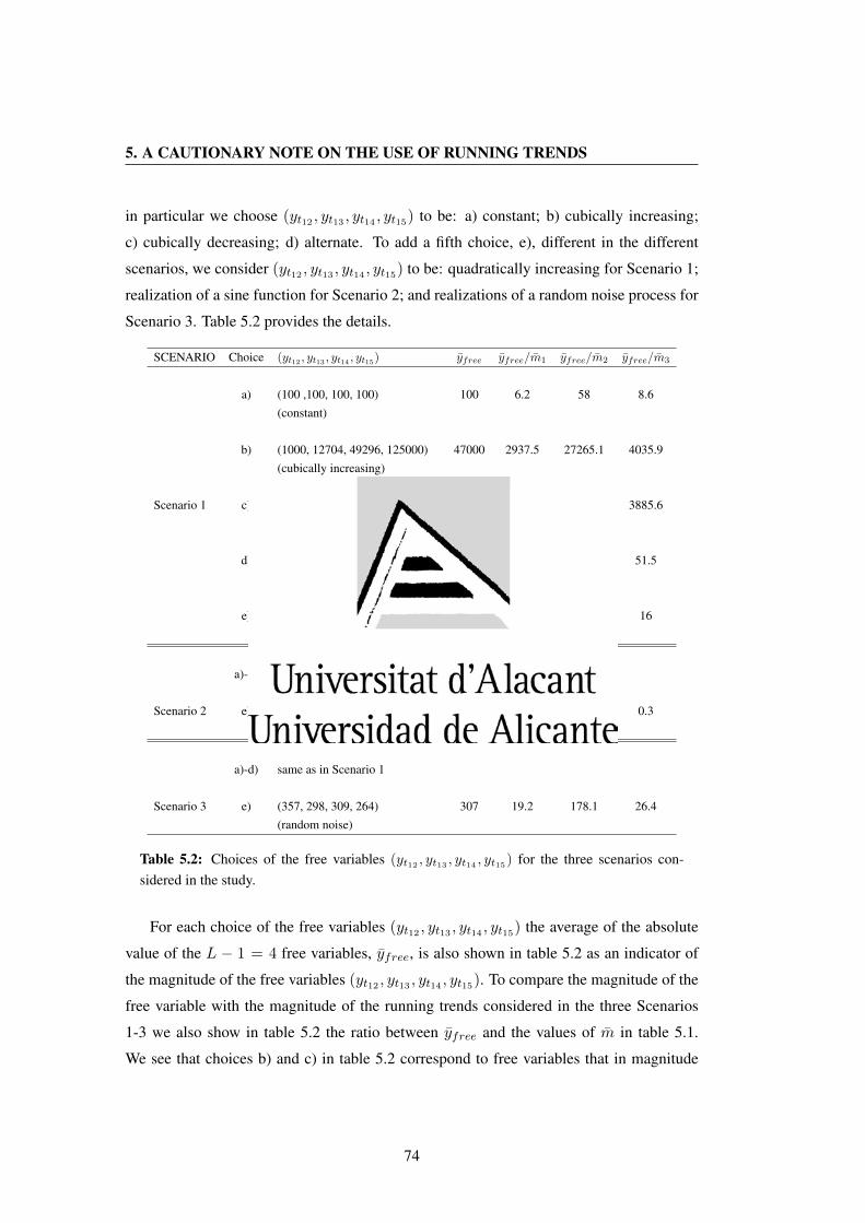
5. A CAUTIONARY NOTE ON THE USE OF RUNNING TRENDS
in particular we choose (yt12 , yt13 , yt14 , yt15) to be: a) constant; b) cubically increasing;
c) cubically decreasing; d) alternate. To add a fifth choice, e), different in the different
scenarios, we consider (yt12 , yt13 , yt14 , yt15) to be: quadratically increasing for Scenario 1;
realization of a sine function for Scenario 2; and realizations of a random noise process for
Scenario 3. Table 5.2 provides the details.
SCENARIO Choice (yt12 , yt13 , yt14 , yt15) yfree yfree/m1 yfree/m2 yfree/m3
a) (100 ,100, 100, 100) 100 6.2 58 8.6(constant)
b) (1000, 12704, 49296, 125000) 47000 2937.5 27265.1 4035.9(cubically increasing)
Scenario 1 c) (1500, -10204, -46796, -122500) 45250 2828.1 26249.9 3885.6(cubically decreasing)
d) (100,1100, 100,1100) 600 37.5 348.1 51.5(alternate)
e) (146,171, 199, 228) 186 11.6 107.9 16(quadratically increasing)
a)-d) same as in Scenario 1
Scenario 2 e) (-2.86, 2.84, 4.35, 3.16) 3.30 0.2 1.9 0.3(sine)
a)-d) same as in Scenario 1
Scenario 3 e) (357, 298, 309, 264) 307 19.2 178.1 26.4(random noise)
Table 5.2: Choices of the free variables (yt12 , yt13 , yt14 , yt15) for the three scenarios con-sidered in the study.
For each choice of the free variables (yt12 , yt13 , yt14 , yt15) the average of the absolute
value of the L − 1 = 4 free variables, yfree, is also shown in table 5.2 as an indicator of
the magnitude of the free variables (yt12 , yt13 , yt14 , yt15). To compare the magnitude of the
free variable with the magnitude of the running trends considered in the three Scenarios
1-3 we also show in table 5.2 the ratio between yfree and the values of m in table 5.1.
We see that choices b) and c) in table 5.2 correspond to free variables that in magnitude
74

5.3 An Illustration
are much larger than the series of running trends for the three Scenarios considered in the
study; while choices a) and d) correspond to choices of the free variables that in magnitude
are moderately larger than the series of running trends for the three Scenarios 1-3. Again,
this will be used later in the discussion of the example.
For each scenario, using the five choice of (yt12 , yt13 , yt14 , yt15) in table 5.2, we gen-
erate five time series in S?h (i.e. five time series with the exactly the same trends series
as in table 5.1). The five time series of length n = 15 for Scenarios 1, 2 and 3 are plot-
ted in figures 5.1, 5.2 and 5.3 respectively. Since each series correspond to a choice of
(yt12 , yt13 , yt14 , yt15), we label the series with the same label as the choice of (yt12 , yt13 , yt14 ,
yt15) in table 5.2. To distinguish the values of the free variables (yt12 , yt13 , yt14 , yt15), from
the rest of the series, in each time series plot (yt12 , yt13 , yt14 , yt15) are represented in red.
Complete details of each series is provided in table 5.3. In each figure we also plot the
series of running trends that they share.
75

5. A CAUTIONARY NOTE ON THE USE OF RUNNING TRENDS
Series (a) Series (b) Series (c) Series (d) Series (e)
-139.72 142005.14 -139984.58 860.28 3.00-17.27 -38372.07 40637.54 -17.27 7.00-82.65 39051.90 -36917.19 917.35 11.00-90.41 75095.12 -72975.94 -90.41 19.00-73.15 85301.54 -83147.84 926.85 27.0017.98 -61456.89 63792.86 17.98 39.00
Scenario 1 -86.84 107377.91 -105251.59 913.16 51.00-24.56 64115.94 -61865.06 -24.56 66.0018.62 22585.62 -20248.38 1018.62 84.0045.75 -18980.25 21371.75 45.75 103.00-32.50 149015.50 -146780.50 967.50 122.00100.00 1000.00 1500.00 100.00 146.00100.00 12704.00 -10204.00 1100.00 171.00100.00 49296.00 -46796.00 100.00 199.00100.00 125000.00 -122500.00 1100.00 228.00
100.97 142245.82 -139743.89 1100.97 5.66107.37 -38247.43 40762.18 107.37 3.9595.61 39230.15 -36738.94 1095.61 0.8092.82 75278.35 -72792.71 92.82 -3.4595.57 85470.25 -82979.12 1095.57 -3.3299.47 -61375.40 63874.35 99.47 -1.9196.72 107561.47 -105068.03 1096.72 4.47
Scenario 2 104.44 64244.94 -61736.06 104.44 4.85103.52 22670.52 -20163.48 1103.52 3.7497.16 -18928.84 21423.16 97.16 -0.4588.48 149136.48 -146659.52 1088.48 -4.75100.00 1000.00 1500.00 100.00 -2.86100.00 12704.00 -10204.00 1100.00 2.84100.00 49296.00 -46796.00 100.00 4.35100.00 125000.00 -122500.00 1100.00 3.16
235.21 142380.07 -139609.64 1235.21 387.0059.00 -38295.81 40713.80 59.00 330.0092.79 39227.34 -36741.76 1092.79 272.0037.61 75223.14 -72847.92 37.61 242.00131.91 85506.59 -82942.78 1131.91 317.0072.94 -61401.94 63847.81 72.94 341.0080.62 107545.37 -105084.13 1080.62 228.00
Scenario 3 86.75 64227.25 -61753.75 86.75 310.0087.50 22654.50 -20179.50 1087.50 295.0039.00 -18987.00 21365.00 39.00 277.00233.00 149281.00 -146515.00 1233.00 373.00100.00 1000.00 1500.00 100.00 357.00100.00 12704.00 -10204.00 1100.00 298.00100.00 49296.00 -46796.00 100.00 309.00100.00 125000.00 -122500.00 1100.00 264.00
Table 5.3: Time series for each of the three scenarios considered.
76

5.3 An Illustration
●
●
●
●
●
●
●
●
●
●
●
2004 2006 2008 2010 2012
1015
2025
Series of running trends: Scenario 1
m.s
tar
●
●
●●
●
●
●
●
●
●
●
● ● ● ●
2002 2004 2006 2008 2010 2012 2014
−10
00
50
(a): R.square= 0.3 % sign. P−value= 0
tS
erie
s (a
)
● ● ● ●
●
●
●
●●
●
●
●
●
●
●
●●
●
●
2002 2004 2006 2008 2010 2012 2014
−50
000
5000
015
0000
(b): R.square= 0 % sign. P−value= 0
t
Ser
ies
(b)
●●
●
●
●
●
●
●●
●
●
●
●
●
●
●●
●
●
2002 2004 2006 2008 2010 2012 2014−15
0000
0
(c): R.square= 0 % sign. P−value= 0
t
Ser
ies
(c) ●
●
●
●
●
●
●
●
●
●
●
●
●
●
●
●
●
●
●
2002 2004 2006 2008 2010 2012 2014
040
080
0
(d): R.square= 0 % sign. P−value= 0
t
Ser
ies
(d)
●
●
●
●
● ● ●●
●●
●●
●
●
●
●
●
●
●
2002 2004 2006 2008 2010 2012 2014
050
150
(e): R.square= 1 % sign. P−value= 100
t
Ser
ies
(e)
●
●
●
●
Figure 5.1: Five series with the same runnig trend series as in Scenario 1. Since each seriescorrespond to a choice (yt12 , yt13 , yt14 , yt15) in table 5.2 we label the series with the same labelas the choice of (yt12 , yt13 , yt14 , yt15) in table 5.2. For each series, the average R-square acrossdifferent windows and the percentage of running trends that are statistically significant at thesignificant level α = 0.05 are denoted by Avg. R-square and % sig. trends respectively.
77

5. A CAUTIONARY NOTE ON THE USE OF RUNNING TRENDS
●
●
●
●●
●
● ●
●
●
●
2004 2006 2008 2010 2012
−2
01
2
Series of running trends: Scenario 2
m.s
tar ●
●
●
●
●
●
●
●●
●
●
● ● ● ●
2002 2004 2006 2008 2010 2012 201490
9510
0
(a): R.square= 0.4 % sign. P−value= 0
t
Ser
ies
(a)
● ● ● ●
●
●
●
●●
●
●
●
●
●
●
●●
●
●
2002 2004 2006 2008 2010 2012 2014
−50
000
5000
015
0000
(b): R.square= 0 % sign. P−value= 0
t
Ser
ies
(b)
●●
●
●
●
●
●
●●
●
●
●
●
●
●
●●
●
●
2002 2004 2006 2008 2010 2012 2014−15
0000
0
(c): R.square= 0 % sign. P−value= 0
t
Ser
ies
(c) ●
●
●
●
●
●
●
●
●
●
●
●
●
●
●
●
●
●
●
2002 2004 2006 2008 2010 2012 2014
200
600
1000
(d): R.square= 0 % sign. P−value= 0
t
Ser
ies
(d)
●
●
●
● ●
●
●
● ●
●
●●
●
●
●
●
●
●
●
2002 2004 2006 2008 2010 2012 2014
−4
02
46
(e): R.square= 0.6 % sign. P−value= 45.45
t
Ser
ies
(e)
●
●
●
●
Figure 5.2: Five series with the same runnig trend series as in Scenario 2. Since each seriescorrespond to a choice (yt12 , yt13 , yt14 , yt15) in table 5.2 we label the series with the same labelas the choice of (yt12 , yt13 , yt14 , yt15) in table 5.2. For each series, the average R-square acrossdifferent windows and the percentage of running trends that are statistically significant at thesignificant level α = 0.05 are denoted by Avg. R-square and % sig. trends respectively.
78

5.3 An Illustration
●
●
●●
● ●
●
●
●
●
●
2004 2006 2008 2010 2012
−20
010
Series of running trends: Scenario 3
m.s
tar
●
●
●
●
●
●● ● ●
●
●
● ● ● ●
2002 2004 2006 2008 2010 2012 2014
5010
020
0
(a): R.square= 0.2 % sign. P−value= 0
tS
erie
s (a
)
● ● ● ●
●
●
●
●●
●
●
●
●
●
●
●●
●
●
2002 2004 2006 2008 2010 2012 2014
−50
000
5000
015
0000
(b): R.square= 0 % sign. P−value= 0
t
Ser
ies
(b)
●●
●
●
●
●
●
●●
●
●
●
●
●
●
●●
●
●
2002 2004 2006 2008 2010 2012 2014−15
0000
0
(c): R.square= 0 % sign. P−value= 0
t
Ser
ies
(c) ●
●
●
●
●
●
●
●
●
●
●
●
●
●
●
●
●
●
●
2002 2004 2006 2008 2010 2012 2014
040
080
012
00
(d): R.square= 0 % sign. P−value= 0
t
Ser
ies
(d)
●
●
●
●
●
●
●
●
●
●
●
●
●
●
●
●
●●
●
2002 2004 2006 2008 2010 2012 2014
250
300
350
(e): R.square= 0.2 % sign. P−value= 9.09
t
Ser
ies
(e)
●
●●
●
Figure 5.3: Five series with the same runnig trend series as in Scenario 3. Since each seriescorrespond to a choice (yt12 , yt13 , yt14 , yt15) in table 5.2 we label the series with the same labelas the choice of (yt12 , yt13 , yt14 , yt15) in table 5.2. For each series, the average R-square acrossdifferent windows and the percentage of running trends that are statistically significant at thesignificant level α = 0.05 are denoted by Avg. R-square and % sig. trends respectively.
79

5. A CAUTIONARY NOTE ON THE USE OF RUNNING TRENDS
5.4 DiscussionDespite its simplicity, the worked example in section 5.3 highlights some importante con-
sequences of the main result in section 5.2. In particular:
1. Time series with a very different behaviour might share exactly the same running
trends series (compare the series (a)-(e) in each of the figures 5.1-5.3). This is true
in general. Different choices of the free variables (ytn−L+2 , ytn−L+3 , . . . , ytn) in the
main result (increasing, decreasing, constant, periodic, etc.), will lead to time series
with the same running trends but whose behaviours are very different. This remark
has two important implications.
First of all, a series of running trends, alone, provides a poor description of the under-
lying time series. That is, a running trends series alone, has a poor performance,
as summary statistics of univariate time series.
Secondly, strong association between running trends series, alone, does not im-
ply any association between the underlying time series. Consider, for example,
the time series (c) and (e) in figure 5.1. Suppose that series (c) represents simulations
of a certain variableX (for the period 2000-2014) from a given model and that series
(e) represents the observed values ofX for the same period. If we use the correlation
between 5-year running trends of series (c) and (e) to assess the model’s perform-
ance, we would conclude that the model performance is very good (the correlation
between the two running trends series is 1 since (c) and (e) share exactly the same
series of running trends). However this result would be misleading. If we compare
the series (c) and (e) we would say that the model’s performance is extremely poor.
The fact that strong association between running trends series, alone, does not imply
any association between the underlying time series is particularly evident if we focus
on the last time window Wn−L+1. According to the main result in section 5.2, in
fact, we can arbitrary fix the value of L− 1 out of the L points in Wn−L+1 and then
use the recursive equation 5.2 to obtain a series with the desired running trends. In
the example above this was exemplified by our arbitrary choice of the free variables
(yt12 , yt13 , yt14 , yt15) in table 5.2.
As an illustration, consider again the time series (c) and (e) in figure 5.1. Suppose
that series (c) represents the time series of a certain variable X (for the period 2000-
80

5.4 Discussion
2014) and that series (e) represents the time series of a certain variable Y for the same
period. The association between the running trends series corresponding to series (c)
and (e) is perfect (since the two time series share the same series of running trends).
However this information, alone, does not tell us anything about the contribution of
X to Y (or the relationship between X and Y ) for the period 2009-2014 (i.e. in the
timeW11) since 4 out of 5 values of each series inW11 are completely unconstrained.
2. Time series with very different running trends series might be almost identical. For
example, compare the series (b) in figures 5.1, 5.2 and 5.3 (or equivalently consider
the time series (b) in table 5.3 corresponding to the the three scenarios). We observe
that the three series are almost identical (the minimum correlation between pair of (b)
series corresponding to two of the three scenarios considered in the study is greater
than 0.999999 !) despite the fact the the corresponding series of running trends are
at best only weakly associated. The implication of this remark is that absence of
association between running trends series does not imply absence of association
between the original series. Once again, consider the series (b) in figure 5.1 and in
figure 5.3. Suppose that series (b) in figure 5.1 represents simulations of a certain
variable X (for the period 2000-2014) from a given model and that series (b) in
figure 5.3 represents the observed values of X for the same period. If we use the
association between 5-year running trends of series (b) in figure 5.1 and series (b)
in figure 5.3 to assess the model’s performance, we would conclude that the model
performance is very poor (the correlation between the two running trends series is
0.035). However this result would be misleading. If we compare the series (c) and
(e) we would say that the model’s performance is excellent.
Again this is true in general and can be explained by the difference in magnitude
between the running trends series and the free variables (ytn−L+2 , ytn−L+3 , . . . , ytn).
Given a series of running trends m?1,m
?2, . . . ,m
?n−L+1, we can always choose the
magnitude of the free variables (ytn−L+2 , ytn−L+3 , . . . , ytn) sufficiently large to make
negligible the contribution of the running trends in the recursive equation in 5.2. Thus
it is possible to have two time series {xt} and {yt} that are almost identical (and
thus that show very high association) but whose running trends series are practically
independent. To build two such time series {xt} and {yt} it would be sufficient to: (i)
generate independently two series of running trends; (ii) then arbitrarily fix the value
81

5. A CAUTIONARY NOTE ON THE USE OF RUNNING TRENDS
of (xtn−L+2 , xtn−L+3 , . . . , xtn) for the first series in such a way that the magnitude of
(xtn−L+2 , xtn−L+3 , . . . , xtn) is much larger than the magnitude of the two series of
running trends and set (ytn−L+2 , ytn−L+3 , . . . , ytn) = (xtn−L+2 , xtn−L+3 , . . . , xtn);
finally (iii) use the vectors of free variables in (ii), the two series of running trends in
(i) and the recursive equation in 5.2 to obtain the desired series {xt} and {yt}. This
is exactly what we did for the (b)-series in our example. The running trend series for
Scenario 1 and 3 were generated independently, and the series (b) where generated
for each Scenario by choosing the magnitude of the free variables much larger than
the magnitude of the corresponding running trends series (compare the value of yfree
and the values of mi for i ∈ {1, 2} in table 5.2). The corresponding (b)-series were
then completed using the recursive formula 5.2.
5.5 Conclusions
Running trends series are widely used as summary statistics for univariate time series and
time series association. In this chapter we obtained an explicit formula for the set of time
series with a given series of running trends and we used this formula to better understand
the limitations of running trend series as descriptive statistics for univariate time series and
time series association. The most important implications of the main result in section 5.2,
as we discussed in the previous section, are that: (i) running trends, alone, provides very
limited information about the underlying time series; and (ii) lack or presence of associ-
ation between the running trends of two time series, alone, tell us almost nothing about
the association of the underlying time series. This should not be interpreted as an argu-
ment against the use of running trends as descriptive statistics for univariate time series
and time series association but rather as a cautionary note on the use of running trends in
applications. It is quite common in descriptive statistics that a descriptive measure, alone,
is of very limited use. For example, a measure of location, like the mean, provides very
limited information about the underlying data set if it is not accompanied by a measure of
dispersion, like the variance, and information about presence of outliers. A small variance,
and absence of outliers, imply that the mean is a representative value of the underlying data
set. While a high variance or the presence of outliers would suggest that the mean is a poor
descriptive statistics for the underlying data set. Thus the question is what are the descript-
ive measures that should accompany the running trends series and that can be used as an
82

5.5 Conclusions
indicator of the performance of running trend series as descriptive statistics for univariate
time series and time series association?. In our understanding such descriptive measures
should be numerical indices that summarize the extent to which the linear models in 5.1
provide a suitable description of the behaviour of the series in each of the overlapping time
windows Wj . One of such measure could be, for example, the average of the n − L + 1
R-squares corresponding to fitting the linear models in 5.1 for each time windows Wj . For
a given time series, the R-square for the time window Wj measures the proportion of the
total variability of the series explained by (the least square estimate of) the linear model in
5.1, thus R-square takes value in [0, 1]. An R-square close (equal) to 1 for a certain time
window Wj would indicate that the time series is approximately (exactly) linear in Wj
and thus the estimated linear trend m?j provides a a very good (perfect) description of the
behaviour of the time series in Wj . The average R-square across different windows (Avg.
R-square) would thus be a natural summary of the overall performance of running trends as
summary statistics. An alternative measure could be the percentage of the n−L+1 running
trends that are statistically significant at the significant level α = 0.05 (% sig. trends). The
value of these two summary statistics has been reported for each series in figures 5.1-5.3.
If we consider figure 5.1 (Scenario 1), for example, we see that according to the average
R-square, and the percentage of running trends that are statistically significant at the sig-
nificant level α = 0.05, running trends as summary statistics, performs very well for the
series (e), and very poorly for all the other series. For series (e) which is quadratically in-
creasing, the average R-square is approximately 1, that means that running trends describe
almost perfectly the behaviour of the series in each time window Wj , and can in fact be
interpreted as acceleration of the underlying series (e). A reconstruction (by integration)
of the original series (e) based on the running trend, in this case, would reproduce almost
perfectly the original series in (e). In terms of time series association, the small (approx-
imately 0) value of the average R-square and of the percentage of running trends that are
statistically significant at the significant level α = 0.05 for series (a)-(d) would imply that
running trend series would provide a very poor measure of association between any pair of
the series in figure 5.1. The definition of suitable measures of the performance of running
trends as summary statistics for univariate time series and time series association can be an
interesting topic for future work. The two examples that I discussed (average R-square and
percentage of statistically significant p-values ) were just used for illustrative purposes, and
83

5. A CAUTIONARY NOTE ON THE USE OF RUNNING TRENDS
further research we think should be done in this direction. Such a research would be relev-
ant not only for the assessment of the performance of running trends as summary statistics
but also for the definition of criteria for the choice of the optimal time window length, L,
to be used in running trend analysis.
84
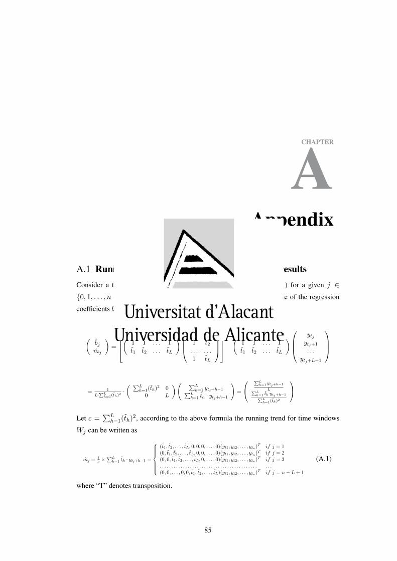
CHAPTER
AAppendix
A.1 Running Trends Analysis: Proof of the Main resultsConsider a time series yt1 , yt2 , . . . , ytn , and the linear model in (5.1) for a given j ∈{0, 1, . . . , n − L} and let th = ∆(2h−1−L2 ). The least square estimate of the regression
coefficients bj and mj are given by:
(bjmj
)=
( 1 1 . . . 1t1 t2 . . . tL
)1 t11 t2. . . . . .1 tL
−1(
1 1 . . . 1t1 t2 . . . tL
)ytjytj+1
. . .ytj+L−1
= 1L·
∑Lh=1(th)
2·( ∑L
h=1(th)2 00 L
)( ∑Lh=1 ytj+h−1∑L
h=1 th · ytj+h−1
)=
∑Lh=1 ytj+h−1
L∑Lh=1 th·ytj+h−1∑L
h=1(th)2
Let c =∑L
h=1(th)2, according to the above formula the running trend for time windows
Wj can be written as
mj = 1c ×
∑Lh=1 th · ytj+h−1 =
(t1, t2, . . . , tL, 0, 0, 0, . . . , 0)(yt1, yt2, . . . , ytn)T if j = 1(0, t1, t2, . . . , tL, 0, 0, . . . , 0)(yt1, yt2, . . . , ytn)T if j = 2(0, 0, t1, t2, . . . , tL, 0, . . . , 0)(yt1, yt2, . . . , ytn)T if j = 3. . . . . . . . . . . . . . . . . . . . . . . . . . . . . . . . . . . . . . . . . . . . .(0, 0, . . . , 0, 0, t1, t2, . . . , tL)(yt1, yt2, . . . , ytn)T if j = n− L+ 1
(A.1)
where “T” denotes transposition.
85

A. APPENDIX
According to formula A.1, the set S? of all time series {yt} = (yt1 , yt2 , . . . , ytn) for which
the corresponding trend series {mj} = (m1, m2, . . . , mn−L+1) is exactly
m?1,m
?2, . . . ,m
?n−L+1 is the solution set of the following linear system with n − L + 1
equations (the number of time windows Wj) and n unknowns (yt1 , yt2 , . . . , ytn).
t1 · yt1 t2 · yt2 . . . tL · ytL = c ·m?
1
t1 · yt2 t2 · yt3 . . . tL · ytL+1 = c ·m?2
t1 · yt3 t2 · yt4 . . . tL · ytL+2 = c ·m?3
. . . . . . . . . . . . . . . . . . . . . . . . . . . . . .t1 · ytn−L+1 t2 · ytn−L+2 . . . tL · ytn = c ·m?
n−L+1
(A.2)
From standard algebra we obtain that solution set of the above system has dimension L−1
and the generic solution of the system is obtained by assigning an arbitrary value to the free
variables (ytn−L+2 , ytn−L+3 , . . . , ytn) and evaluating the rest of the variable using back-
substitution in formula A.2. This leads to the recursive formula:
yn−L+1−j =c
t1·m?
n−L+1−j −L−1∑h=1
ytn−L+1−j+h · th, j = 0, 1, . . . , n− L
Once we have arbitrarly fixed the values of (ytn−L+2 , ytn−L+3 , . . . , ytn), then:
• for j = 0 the recursive formula above provides the value of ytn−L+1 as a function of
(ytn−L+2 , ytn−L+3 , . . . , ytn).
• for j = 1 the recursive formula above provides the value of ytn−L as a function of
(ytn−L+1 , ytn−L+2 , . . . , ytn−1). And so on.
86

References
Altamimi, Z., X. Collilieux, J. Legrand, B. Garayt, and C. Boucher, 2007: ITRF2005:
A new release of the International Terrestrial Reference Frame based on time series of
station positions and Earth Orientation Parameters. J. Geophys. Res., 112, B09 401, doi:
10.1029/2007JB004949. 19
Altamimi, Z., X. Collilieux, and L. Metivier, 2011: ITRF2008: an improved solu-
tion of the International Terrestrial Reference Frame. J. Geod., 85, 457–473, doi:
10.1007/s00190-011-0444-4. xii, 15, 19
Altamimi, Z., P. Sillard, and C. Boucher, 2002: ITRF2000: A new release of the Interna-
tional Terrestrial Reference Frame for Earth science applications. J. Geophys. Res., 107,
ETG 2–1 ETG 2–19, doi:10.1029/2001JB000561. 19
Belda, S., J. Bohm, and J.-M. Ferrandiz, 2014a: Improvements in EOPs and baseline es-
timation using the future RAEGE network. Geophys. Res. Abstr. EGU2014-9997, 35. ix,
6
Belda, S., D. Garcıa-Garcıa, and J.-M. Ferrandiz, 2014b: On the decorrelation filtering of
RL05 GRACE data for global applications. Geophys. J. Int., 200, 173–184, doi:10.1093/
gji/ggu386.
Belda, S., R. Heinkelmann, J.-M. Ferrandiz, T. Nilsson, and H. Schuh, 2015a: A new
empirical model for Free Core Nutation. Geophys. Res. Abstr. EGU2015-11088, 17.
Belda, S., R. Heinkelmann, J.-M. Ferrandiz, T. Nilsson, and H. Schuh, 2015b: On the con-
sistency of the current conventional EOP series and the Celestial and Terrestrial reference
frames. J. Geod., In review.
87

REFERENCES
Belda, S., and Coauthors, 2014c: Reference frame induced long-term effects on EOP.
Geodaetische Woche.
Bettadpur, B., 2012: CSR Level-2 processing standards document for product release 05.
GRACE 327-742, Revison 4.0. 47
Blewitt, G., and Coauthors, 2010: Geodetic Observations and Global Reference Frame
Contributions to Understanding Sea-Level Rise and Variability. Understanding Sea-
Level Rise and Variability, Chapter, 9, doi:10.1002/9781444323276.ch9. x, 9
Bloßfeld, M., M. Seitz, and D. Angermann, 2014: Non-linear station motions in epoch and
multi-year reference frames. J. Geod., 88, 46–63, doi:10.1007/s00190-013-0668-6. 32
Bockmann, S., T. Artz, and A. Nothnagel, 2010: VLBI Terrestrial Reference Frame contri-
butions to ITRF2008. J. Geod., 84, 201–219, doi:10.1007/s00190-009-0357-7. 19
Bohm, J., S. Bohm, A. Pany, L. Plank, H. Spicakova, T. Teke, and H. Schuh, 2012: The
new Vienna VLBI Software VieVS. Geodesy for Planet Earth, Proc. of the 2009 IAG
Symp., 1007–1011, doi:10.1007/978-3-642-20338-1 126. xii, 18
Bohm, J., B. Werl, and H. Schuh, 2006: Troposphere mapping functions for GPS and very
long baseline interferometry from European Centre for Medium-Range Weather Fore-
casts operational analysis data. J. Geophys. Res., 1111, B2, doi:10.1029/2005JB003629.
18
Bradley, B., D. Vallado, A. Sibois, and P. Axelrad, 2012: Earth Orientation Parameter
Considerations for Precise Spacecraft operations. Astronaut. Sci., 142, 13. 1
Campbell, J., 2000: From Quasars to Benchmarks: VLBI Links Heaven and Earth. IVS
2000 General Meeting Proc., CP-2000-209893. 3
Cannon, W., 1999: Overview of VLBI. International VLBI Service for Geodesy and Astro-
nomy 1999 Annual Report, TP-1999-209243. viii, 4
Capitaine, N., P. Mathews, V. Dehant, P. Wallace, and S. Lambert, 2009: On the IAU
2000/2006 precession–nutation and comparison with other models and VLBI observa-
tions. Celest. Mech. Astron., 103, 179–190, doi:10.1007/s10569-008-9179-9. 37
88

REFERENCES
Capitaine, N., P. Wallace, and J. Chapront, 2003: Expressions for IAU 2000 precession
quantities. Astron. Astrophys., 412, 567–586, doi:10.1051/0004-6361:20031539. 36
Cazenave, A., and J. Chen, 2010: Time-variable gravity from space and present-day mass
redistribution in the Earth system. Earth and Planet. Sci. Lett., 298, 263–274, doi:10.
1016/j.epsl.2010.07.035. 12
Chambers, D., 2006: Evaluation of new GRACE time-variable gravity data over the ocean.
Geophys. Res. Lett., 33, L17 603, doi:10.1029/2006GL027296. 12, 48, 49, 50
Chambers, D., and J. Bonin, 2012: Evaluation of Release-05 GRACE time-variable
gravity coefficients over the Ocean. Ocean Sci. Discuss., 9, 2187–2214, doi:10.5194/
os-8-859-2012. xxiv, 48, 50, 65, 66, 67
Chao, B., 1994: The Geoid and Earth rotation. Geoid and its geophysical Interpretations,
ed. P. Vanicek and N. Christou, 285–298. x, 7, 8
Chao, B., 2005: On inversion for mass distribution from global (time variable) gravity field.
J. Geodyn., 39, 223–230, doi:10.1016/j.jog.2004.11.001. xx, xxi, 47, 49
Chen, J., C. Wilson, and K. Seo, 2006: Optimized smoothing of gravity recovery and
climate experiment (GRACE) time-variable gravity observations. J. Geophys. Res, 111,
B06 408, doi:10.1029/2005JB004064. 48
Chen, J., C. Wilson, B. Tapley, and S. Grand, 2007: Grace detects coseismic and post-
seismic deformation from the Sumatra-Andaman earthquake. Geophys. Res. Lett., 34,
L13 302, doi:10.1029/2007GL030356. xxi, xxii, xxiv, 48, 49, 50, 59, 62, 65, 67
Chen, J., C. Wilson, and Y. Zhou, 2012: Seasonal excitation of polar motion. J. Geod., 62,
8–15, doi:10.1016/j.jog.2011.12.002. 7
Cheng, M., and J. Ries, 2007: GRACE technical note 05: monthly estimates of C20 from
5 SLR satellites. Available at: http://podaac.jpl.nasa.gov/grace/documentation. 49
Cummins, P., and J. Wahr, 1993: A study of the Earth’s free core nutation using IDA gravity
data. J. Geophys. Res., 98, 2091–2104, doi:10.1029/92JB01956. 34
89

REFERENCES
Dahle, C., F. Flechtner, C. Gruber, D. Konig, R. Konig, G. Michalak, and K.-H. Neumayer,
2013: GFZ GRACE level-2 processing standards document for level-2 product release
0005. Available at: http://podaac.jpl.nasa.gov/gravity/grace-documentation. 47
Defraigne, P., V. Dehant, and P. Paquet, 1995: Link between the Retrograde-Prograde
Nutations and Nutations in Obliquity and Longitude. Celest. Mech. Dyn. Astron., 62,
363–376, doi:10.1007/BF00692286. 34
Dehant, V., 2002: Report of the IAU working group on ’Nonrigid-Earth Nutation Theory’.
Highlights of Astron., 12, 117–119. 22
Dehant, V., O. Viron, and J. Barriot, 2005: Geophysical excitation of the Earth orientation
parameters EOP and its contribution to GGOS. J. Geodyn., 40, 394–399, doi:10.1016/j.
jog.2005.06.004. ix, 5
Duan, X., J. Guo, C. Shum, and W. Van der Wal, 2009: On the postprocessing removal of
correlated errors in GRACE temporal gravity field solutions. J. Geod., 83, 1095–1106,
doi:10.1007/s00190-009-0327-0. xxi, xxiv, 48, 49, 50, 53, 65, 66, 67
Feissel, M., and Coauthors, 2013: Earth Orientation and related Reference Frames.
Contributions of Space Geodesy to Geodynamics: Earth Dynamics, 24, 99–111, doi:
10.1029/GD024p0099.
Ferrandiz, J.-M., and R. Gross, 2014: The new IAU/IAG Joint Working Group on Theory
of Earth Rotation. Proc. of the IAG Symp. (to appear), 143. 27
Fey, A. L., and Coauthors, 2004: The Second Extension of the International Celestial
Reference Frame: ICRF-EXT.1. Astron. J., 127, 3587, doi:10.1086/420998. xii, 15, 19
Florsch, N., and J. Hinderer, 2000: Bayesian estimation of the free core nutation parameters
from the analysis of precise tidal gravity data. Phys. Earth Planet. Inter., 117, 21–35,
doi:10.1016/S0031-9201(99)00084-9. 34
Furuya, M., Y. Hamano, and I. Naito, 1996: Quasi-periodic wind signal as a possible
excitation of Chandler wobble. J. Geophys. Res., 101, 25 537–25 546, doi:10.1029/
96JB02650. 45
90
REFERENCES
Garcıa-Garcıa, D., B. Chao, and J.-P. Boy, 2010: Steric and mass-induced sea level
variations in the Mediterranean Sea. J. Geophys. Res., 115, C12 016, doi:10.1029/
2009JC005928. 48
Getino, J., and J.-M. Ferrandiz, 2000: Accurate analytical nutation series. Mon. Not. R.
Astr. Soc., 306, L45–L49, doi:10.1046/j.1365-8711.1999.02741.x. 36
Gross, R., 2000: The excitation of the Chandler wobble. Geophys. Res. Lett., 27, 2329–
2332, doi:10.1029/2000GL011450. 45
Gwinn, C., T. Herring, and I. Shapiro, 1986: Geodesy by radio interferometry: Studies
of the forced nutations of the Earth: 2. interpretation. J. Geophys. Res., 91, 4755–4765,
doi:10.1029/JB091iB05p04755. 34
Hamlington, B. D., M. W. Strassburg, R. R. Leben, W. Han, R. S. Nerem, and K.-Y. Kim,
2014: Uncovering an antropogenic sea-level rise signal in the Pacific ocean. Nat. Clim.
Change, 4, 782–785, doi:10.1038/nclimate2307. xxiv, 70
Hamlington, B. D., M. W. Strassburg, R. R. Leben, R. S. Nerem, and K.-Y. Kim, 2013:
Contribution of the Pacific Decadal Oscillation to global mean sea level trends. Geophys.
Res. Lett., 40, 5171–5175, doi:10.1002/grl.50950. xxiv, 70
Heinkelmann, R., S. Belda, J.-M. Ferrandiz, and H. Schuh, 2014a: The consistency of the
current conventional Celestial and Terrestrial Reference Frames and the conventional
EOP series. Journ. 2014 Systemes de reference spatio-temporels, In print.
Heinkelmann, R., S. Belda, J.-M. Ferrandiz, and H. Schuh, 2014b: How consistent are the
current conventional Celestial and Terrestrial Reference Frames and the conventional
Earth orientation parameters? IAG Symp. Series REFAG 2014 Proc., In review.
Heinkelmann, R., T. Nilsson, M. Karbon, V. Raposo-Pulido, B. Soja, and H. Schuh, 2014c:
Reference frame-induced error in VLBI Earth orientation determinations. Geophy. Res.
Abst., 16, EGU2014–5107. 18
Heiskanen, W., and H. Moritz, 1967: Physical Geodesy. Book. 12
Herring, T., C. Gwinn, and I. Shapiro, 1986: Geodesy by radio interferometry: Studies of
the forced nutations of the Earth: 1. Data analysis. J. Geophys. Res., 91, 4745–4754,
doi:10.1029/JB091iB05p04745. 34
91
REFERENCES
Hilton, J., and Coauthors, 2006: Report of the International Astronomical Union Division I
Working Group on Precession and the Ecliptic. Celest. Mech. Dyn. Astron., 94, 351–367,
doi:10.1007/s10569-006-0001-2. 22
Holgate, S. J., and P. L. Woodworth, 2004: Evidence for enhanced coastal sea level rise
during the 1990s. Geophys. Res. Lett., 31, L07 305, doi:10.1029/2004GL019626. xxiv,
69
Jekeli, C., 1981: Alternative methods to smooth the Earth’s gravity field. Department of
Geod. Sci. and Surv., Ohio State Univ. (Columbus). xx, 12, 48
Kierulf, H., and H. Plag, 2006: Precise point positioning requires consistent global
products. EUREF Publication No. 14, 35, 111. viii, 3
Krasna, H., J. Bohm, and H. Schuh, 2013: Free Core Nutation observed by VLBI. Astron.
Astrophys., 555, A29, doi:10.1051/0004-6361/201321585. x, xvii, xviii, xix, 9, 12, 23,
34, 36, 43, 44, 45
Lambert, S., 2007: Empirical model of the Free Core Nutation. Technical note available at
http://syrte.obspm.fr/. x, xvii, xix, 9, 12, 23, 34, 36, 43
Lambert, S., and V. Dehant, 2007: The Earth’s core parameters as seen by the VLBI.
Astron. and Astrophys., 469, 777–781, doi:10.1051/0004-6361:20077392. 35
Landerer, F., and S. Swenson, 2012: Accuracy of scaled GRACE terrestrial water storage
estimates. Water Resour. Res., 48, W04 531, doi:10.1029/2011WR011453. 57
Ma, C., E. F. Arias, T. Eubanks, A. Fey, A.-M. Gontier, C. Jacobs, O. S. . B. Archinal, and
P. Charlot, 1998: The International Celestial Reference Frame as Realized by Very Long
Baseline Interferometry. Astron. J., 116, 516, doi:10.1086/300408. 19
Ma, C., and Coauthors, 2009: The Second Realization of the International Celestial Refer-
ence Frame by Very Long Baseline Interferometry. IERS Technical Note, No. 35, 1–204.
xvii, 12, 19
Malkin, Z., 2004: Comparison of VLBI nutation series with the IAU2000A model. Proc.
of Journ. 2003: Astrom., Geodyn. and Solar System Dyn.: from milliarcseconds to mi-
croarcseconds, Eds. A. Finkelstein, N. Capitaine, 24–31.
92

REFERENCES
Malkin, Z., 2007: Empirical Models of the Earth’s Free Core Nutation. Sol. Syst. Res., 41
(6), 492–497, doi:10.1134/S0038094607060044.
Malkin, Z., 2010: Comparison of CPO and FCN empirical models. In: Proc. Journ. 2010:
New challenges for reference systems and numerical standards in astronomy, ed. N.
Capitaine, 172–175. x, 9, 23, 36
Malkin, Z., 2013: Free core nutation and geomagnetic jerks. J. Geodyn., 72, 53–58, doi:
10.1016/j.jog.2013.06.001. 23
Mathews, P., T. Herring, and B. Buffet, 2002: Modeling of nutation and precession: New
nutation series for nonrigid Earth and insights into the earth’s interior. J. Geophys. Res.,
107, 3–1–3–26, doi:10.1029/2001JB000390. 36
Moritz, H., and I. Mueller, 1987: Earth Rotation. Theory and observation. Ung. Publ. New
York. 7
Nilsson, T., R. Heinkelmann, M. Karbon, V. Raposo-Pulido, B. Soja, and H. Schuh, 2014:
Earth Orientation Parameters estimated from VLBI during the CONT11 campaign. J.
Geod, 88, 491–502, doi:10.1007/s00190-014-0700-5. xiii, 18
Palmer, M. D., and D. J. McNeall, 2014: Internal variability of Earth’s energy budget simu-
lated by CMIP5 climate models. Environ. Res. Lett., 9, 034 016, doi:10.1088/1748-9326/
9/3/034016. xxiv, 70
Paulson, A., S. Zhong, and J. Wahr, 2007: Inference of mantle viscosity from GRACE and
relative sea level data. Geophys. J. Int. 53
Peters, T., J. Muller, and N. Sneeuw, 2002: Temporal variations in the Earth’s gravity field
with emphasis on atmospheric effects. Schuh, H.; Soffel, M.; Hornik, H. (eds.) Vortrage
beim 4. DFG-Rundgesprach im Rahmen des Forschungsvorhabens ’Rotation der Erde’,
118, 133–140. x, 7
Petit, G., and B. Luzum, 2010: IERS convention 2010. IERS Technical Note, 36. vii, xiii,
1, 2, 36
Petrachenko, B., 2009: Progress Report of the IVS VLBI2010 Committee: Desing Aspects
of the VLBI2010 System. Technical report, IVS VLBI 2010 Committee. ix, 5
93

REFERENCES
Plag, H., and M. Pearlman, 2009: Global Geodetic Observing System: Meeting the Re-
quirements of a Global Society on a Changing Planet in 2020. Springer, 332 pages,
doi:978-3-642-02687-4. 11, 27
Richter, B., 1988: Chandler effect and Nearly Diurnal Free Wobble as determined from ob-
servations with superconducting gravimeter. Proc. 128 IAU Symp., Kluwer Academic,
309–315. 34
Risbey, J. S., S. Lewandowsky, C. Langlais, D. P. Monselesan, T. J. O’Kane, and
N. Oreskes, 2014: Well-estimated global surface warming in climate projections se-
lected for ENSO phase. Nat. Clim. Change, 4, 835–840, doi:10.1038/nclimate2310. 70
Rodell, M., K. Mitchell, M. Bosilovich, D. Toll, and D. Lohmann, 2004: The global land
data assimilation system. Bull. am. Meteorol. Soc., 85(3), 381–394. 53
Santer, B. D., and Coauthors, 2014: Volcanic contribution to decadal changes in tropo-
spheric temperature. Nat. Geosci., 7, 185–189, doi:10.1038/ngeo2098. xxiv, 70
Schuh, H., and D. Behrend, 2012: VLBI: A fascinating technique for Geodesy and astro-
metry. J. Geodyn., 61, 68–80, doi:10.1016/j.jog.2012.07.007. 4
Schuh, H., and J. Bohm, 2013: Sciences of Geodesy. G.Xu (ed.), Springer-Verlag Berlin
Heidelberg. viii, ix, 3, 5
Schuh, H., B. Richter, and S. Nagel, 2000: Analysis of Long Time Series of Polar Mo-
tion. Polar Motion: Historical and Scientific Problems. ASP Conference Series. IAU
Colloquium, 208, 321, doi:1-58381-039-0. 34
Seitz, M., D. Angermann, M. Blobfeld, H. Drewes, and M. Gerstl, 2012: The 2008
DGFI realization of the ITRS: DTRF2008. J. Geod, 86, 1097–1123, doi:10.1007/
s00190-012-0567-2.
Shirai, T., and T. Fukushima, 2000a: Improvement of Nonrigid-Earth Nutation Theory by
adding a Model Free Core Nutation Term. Proc. of IAU Colloquium, 180, 223–229. 34
Shirai, T., and T. Fukushima, 2000b: Numerical convolution in the time domain and its
application to the nonrigid-Earth nutation theory. Astron. J., 119, 2475–2480, doi:10.
1086/301359. 34
94

REFERENCES
Shirai, T., and T. Fukushima, 2001: Construction of a new forced nutation theory of nonri-
gid Earth. Astron. J., 121, 3270–3283, doi:10.1086/321067. 36
Smith, M., 1977: Wobble and nutation of the Earth. Geophys. J. R. Astron. Soc., 50, 103–
140, doi:10.1111/j.1365-246X.1977.tb01326.x. xvi, 33
Stammer, D., C. Wunsch, I. Fukumori, and J. Marshall, 2002: State estimation in modern
oceanographic research. Trans. Am. Geophys. Un., 83, 294–295. 53
Sun, J., J. Bohm, T. Nilsson, H. Krasna, S. Bohm, and H. Schuh, 2014: New VLBI2010
scheduling strategies and implications on the terrestrial reference frames. J. Geod., 88. 6
Swenson, S., and J. Wahr, 2002: Methods for inferring regional surface mass anom-
alies from Gravity Recovery and Climate Experiment (GRACE) measurements of time-
variable gravity. J. Geophys. Res., 107(B9), 2193, doi:10.1029/2001JB000576. xx, 48,
56
Swenson, S., and J. Wahr, 2006: Post-processing removal of correlated errors in GRACE
data. J. Geophy. Res., 33, L08 402, doi:10.1029/2005GL025285. xx, xxi, 12, 48, 49
Tapley, B., S. Bettadpur, M. Watkins, and C. Reigber, 2004: The Gravity Recovery and Cli-
mate Experiment: Mission overview and early results. Geophys. Res. Lett., 31, L09 607,
doi:10.1029/2004GL019920. 9
Toomre, A., 1974: On the Nearly Diurnal Wobble of the Earth. Geophys. J. R. Astron. Soc.,
38, 335–348, doi:10.1111/j.1365-246X.1974.tb04126.x. xvi, 33
Trottini, M., I. Vigo, and S. Belda, 2015: On the use of Running Trends as Summary
Statistics for Univariate Time Series and Time Series Association. J. Clim., In review.
Velicogna, I., and J. Wahr, 2006: Measurements of time-variable gravity show mass loss in
Antarctica. Sci., 311, 1754–1756. 57
VondraK, J., and C. Ron, 2014: Geophysical excitation of nutation - comparison of dif-
ferent models. Acta Geodyn. Geomater, 11 No. 3 (175), 193–200, doi:10.13168/AGG.
2014.0007. 23
95

REFERENCES
Wahr, J., 1981: The forced nutations of an elliptical, rotating, elastic and oceanless Earth.
Geophys. J. R. Astron. Soc., 64, 705–727, doi:10.1111/j.1365-246X.1981.tb02691.x.
xvii, 33
Wahr, J., M. Molenaar, and F. Bryan, 1998: Time-variability of the Earth’s gravity field:
hydrological and oceanic effects and their possible detection using GRACE. J. Geophys.
Res., 103, 30 205–30 229. xx, xxi, 47, 49, 56
Watkins, M., and D.-N. Yuan, 2012: JPL level-2 processing standards document for level-2
product release 05, revision 5.0. Available at: http://podaac.jpl.nasa.gov/gravity/grace-
documentation, Revision 5.0. 47
Watts, R., and M. Morantine, 1991: Is the greenhouse gas-climate signal hiding in the deep
ocean. Clim. Change, 18(4), iii–vi, doi:10.1007/BF00142966. xi, 10
Zhang, Z., B. Chao, Y. Lu, and H. Hsu, 2009: An effective filtering for GRACE
time-variable gravity: fan filter. Geophys. Res. Lett., 36, L17 311, doi:10.1029/
2009GL039459. xx, xxiii, 13, 48, 64
96

Acronyms
AAM Atmospheric angular momentum
AC Analysis Centers
CHAMP Challenging Minisatellite Payload
CIO Celestial Intermediate Origin
CIP Celestial Intermediate Pole
CMIP5 Couple Model Intercomparison Project 5
CRF Celestial Reference Frame
CSR Center for Space Research
DORIS Doppler Orbitography Integrated by Satellite
ECCO Estimating the Circulation and Climate of the Ocean
EOP Earth Orientation Parameters
ERA Earth rotation angle
ERP Earth Rotation Parameters
FCN Free Core Nutation
FICN Free Inner Core Nutation
GCRS Geocentric Celestial Reference System
GEO Group on Earth Observations
97

ACRONYMS
GEOSS Global Earth Observing System of Systems
GFZ GeoForschungsZentrum
GGOS Global Geodetic Observing System
GLDAS Global Land Data Assimilation Systems
GMSL Global Mean Sea Level
GMST Global mean surface air temperature
GNSS Global Navigation Satellite Systems
GOCE Gravity Field and Steady-State Ocean Circulation Explorer)
GRACE Gravity Recovery
GST Global surface temperature
HAM Hydrological angular momentum
IAG International Association of Geodesy
ICRF International Celestial Reference Frames
ICRF2 International Celestial Reference Frame 2
ICRS International Celestial Reference System
IERS International Earth Rotation and Reference System Service
IGS International GNSS Service
ITRF International Terrestrial Reference Frames
ITRS International Terrestrial Reference System
JGW Joint Working Group
JPL Jet Propulsion Laboratory
LOD Length of day
98
ACRONYMS
LS Least Squares
NDFW Nearly Diurnal Free Wobble
NNR No Net Rotation
OAM Oceanic angular momentum
OBP Ocean Bottom Pressure
OHC Ocean heat
PDO Pacific Decadal Oscillation
PGR Post Glacial Rebound
PM Polar Motion
POD Precise Orbit Determination
RAEGE New Atlantic Network of Geodynamical and Space Stations
RL04 Release 04
RL05 Release 05
rms Root Mean Square
RTA Running Trend Analysis
SC Stokes coefficients
SD Standard Deviation
SLP Sea Level Pressure
SLR Satellite Laser Ranging
SLV Sea Level Variation
TE Earth System
TIO Terrestrial Intermediate Origin
99

ACRONYMS
TRF Terrestrial Reference Frame
TWS Terrestrial Water Storage
USNO United States Naval Observatory
UT1 Universal Time
VieVS Vienna VLBI Software
VLBI Very Long Baseline Interferometry
VMF1 Vienna Mapping Functions
WM Weighted Mean
WRMS Weighted Root Mean Square
WTE Water Thickness equivalent
100
Declaration
I herewith declare that I have produced this work without the prohibited assist-
ance of third parties and without making use of aids other than those specified;
notions taken over directly or indirectly from other sources have been iden-
tified as such. This work has not previously been presented in identical or
similar form to any examination board.
The dissertation work was conducted from 2011 to 2015 under the supervision
of Jose Manuel Ferrandiz Leal at the University of Alicante.
Alicante,

This dissertation was finished writing in Alicante on Tuesday 1st September, 2015
