contributions to functional data analysishss.ulb.uni-bonn.de/2018/5070/5070.pdf · 2018-05-18 ·...
TRANSCRIPT

Contributions to Functional Data Analysis
With a Focus on
Points of Impact in Functional Regression
Inaugural-Dissertation
zur Erlangung des Grades eines Doktors
der Wirtschafts- und Gesellschaftswissenschaften
durch die
Rechts- und Staatswissenschaftliche Fakultät
der Rheinischen Friedrich-Wilhelms-Universität Bonn
vorgelegt von
Dominik Johannes Poß
aus Koblenz
2018

Dekan: Prof. Dr. Daniel Zimmer, LL.M.
Erstreferent: Prof. Dr. Alois Kneip
Zweitreferent: JProf. Dr. Dominik Liebl
Tag der mündlichen Prüfung: 03.05.2018

i
Contents
Page
Contents i
List of Figures iii
List of Tables v
Acknowledgments vii
Introduction 1
1 Functional Linear Regression with Points of Impact 3
1.1 Introduction . . . . . . . . . . . . . . . . . . . . . . . . . . . . . . . . . . . . . . . . . . 3
1.2 Identifiability . . . . . . . . . . . . . . . . . . . . . . . . . . . . . . . . . . . . . . . . . . 7
1.3 Non-smooth covariance functions . . . . . . . . . . . . . . . . . . . . . . . . . . . . . 10
1.4 Estimating points of impact . . . . . . . . . . . . . . . . . . . . . . . . . . . . . . . . . 12
1.5 Parameter estimates . . . . . . . . . . . . . . . . . . . . . . . . . . . . . . . . . . . . . 18
1.6 Simulation study . . . . . . . . . . . . . . . . . . . . . . . . . . . . . . . . . . . . . . . 20
1.7 Application to real data . . . . . . . . . . . . . . . . . . . . . . . . . . . . . . . . . . . 22
1.8 Proofs of some theorems . . . . . . . . . . . . . . . . . . . . . . . . . . . . . . . . . . . 25
Supplement to:
Functional Linear Regression with Points of Impact 33
Appendix A Application to near infrared data . . . . . . . . . . . . . . . . . . . . . . . 33
Appendix B Approximation properties of eigenfunctions . . . . . . . . . . . . . . . . 35
Appendix C Additional proofs . . . . . . . . . . . . . . . . . . . . . . . . . . . . . . . . . 37

ii CONTENTS
2 Points of Impact in Generalized Linear Models with Functional Predictors 53
2.1 Introduction . . . . . . . . . . . . . . . . . . . . . . . . . . . . . . . . . . . . . . . . . . 53
2.2 Determining points of impact . . . . . . . . . . . . . . . . . . . . . . . . . . . . . . . . 55
2.2.1 Estimation . . . . . . . . . . . . . . . . . . . . . . . . . . . . . . . . . . . . . . . 60
2.2.2 Asymptotic results . . . . . . . . . . . . . . . . . . . . . . . . . . . . . . . . . . 61
2.3 Parameter estimation . . . . . . . . . . . . . . . . . . . . . . . . . . . . . . . . . . . . . 62
2.4 Practical implementation . . . . . . . . . . . . . . . . . . . . . . . . . . . . . . . . . . 65
2.5 Simulation . . . . . . . . . . . . . . . . . . . . . . . . . . . . . . . . . . . . . . . . . . . 66
2.6 Points of impact in continuous emotional stimuli . . . . . . . . . . . . . . . . . . . . 71
Supplement to:
Points of Impact in Generalized Linear Models with Functional Predictors 75
Appendix A Additional simulation results . . . . . . . . . . . . . . . . . . . . . . . . . . 75
Appendix B Proofs of the theoretical results from Section 2.2 . . . . . . . . . . . . . 78
Appendix C Proofs of the theoretical results from Section 2.3 . . . . . . . . . . . . . 86
Appendix D Extending the linear predictor . . . . . . . . . . . . . . . . . . . . . . . . . 108
D.1 Parameter estimates: IV approach . . . . . . . . . . . . . . . . . . . . . . . . 109
D.2 Parameter estimates: comprehensive approach . . . . . . . . . . . . . . . . 110
D.3 Simulation study for the extended model . . . . . . . . . . . . . . . . . . . . 113
D.4 Proofs of the theoretical results from Appendix D . . . . . . . . . . . . . . . 119
3 Analysis of juggling data 123
3.1 Introduction . . . . . . . . . . . . . . . . . . . . . . . . . . . . . . . . . . . . . . . . . . 123
3.2 Registering the juggling data . . . . . . . . . . . . . . . . . . . . . . . . . . . . . . . . 124
3.2.1 Analyzing the principal components . . . . . . . . . . . . . . . . . . . . . . . 127
3.2.2 Analyzing the principal scores . . . . . . . . . . . . . . . . . . . . . . . . . . . 128
3.3 Summary . . . . . . . . . . . . . . . . . . . . . . . . . . . . . . . . . . . . . . . . . . . . 132
References 133

iii
List of Figures
Page
1.1 Decomposition of a trajectory from a Brownian motion . . . . . . . . . . . . . . . . 8
1.2 Empirical covariance between Zδ(t) and Y in dependence of δ . . . . . . . . . . . 14
1.3 Estimating points of impact using Canadian weather data . . . . . . . . . . . . . . 23
A.1 Estimating points of impact using NIR data . . . . . . . . . . . . . . . . . . . . . . . 34
B.1 An odd function with periodicity 4 . . . . . . . . . . . . . . . . . . . . . . . . . . . . 36
2.1 Self-reported feeling trajectories . . . . . . . . . . . . . . . . . . . . . . . . . . . . . . 55
2.2 Illustrating estimation of points of impact . . . . . . . . . . . . . . . . . . . . . . . . 59
2.3 Estimation errors for DGP 1 (1 impact point, BIC vs LMcK) . . . . . . . . . . . . . 68
2.4 Estimation errors for DGP 2 (2 impact points, BIC vs TRH) . . . . . . . . . . . . . 69
2.5 Estimation errors for DGP 4 (2 impact points, BIC vs TRH, GCM) . . . . . . . . . 70
A.1 Estimation errors for DGP 3 (4 impact points, BIC vs TRH) . . . . . . . . . . . . . 76
A.2 Estimation errors for DGP 5 (2 impact points, BIC vs TRH, EBM) . . . . . . . . . . 77
D.1 Estimation errors for simulation model β(t)≡ 0 (2 impact points) . . . . . . . . . 117
D.2 Estimation errors for simulation model β(t) 6= 0 (2 impact points) . . . . . . . . . 118
3.1 A landmarked juggling trial along the z direction . . . . . . . . . . . . . . . . . . . 125
3.2 (Registered) juggling cycles for the x , y and z direction . . . . . . . . . . . . . . . 125
3.3 The deformation functions . . . . . . . . . . . . . . . . . . . . . . . . . . . . . . . . . 126
3.4 FPCA of the spatial directions x ,y ,z . . . . . . . . . . . . . . . . . . . . . . . . . . . . 127
3.5 Evolution of the scores for the juggling cycles over the trials . . . . . . . . . . . . . 129


v
List of Tables
Page
1.1 Estimation errors for different sample sizes (2 impact points, FLR) . . . . . . . . . 21
1.2 Results of fitting competing PoI models using the Canadian weather data . . . . 24
A.1 Results of fitting competing PoI models using NIR data . . . . . . . . . . . . . . . . 34
2.1 DGP settings for the simulation study . . . . . . . . . . . . . . . . . . . . . . . . . . . 67
2.2 Estimation results using emotional stimuli data . . . . . . . . . . . . . . . . . . . . . 73
D.1 Estimation errors for different sample sizes (2 impact points, GFLR) . . . . . . . . 115
3.1 Variation of the j-th principal component due to the l-th spatial direction . . . . 128
3.2 Estimated coefficients from a quadratic regression of the scores on the trials . . . 130
3.3 Correlation between the scores of W and the juggling cycles . . . . . . . . . . . . 131
3.4 Results from a regression of the cycle scores . . . . . . . . . . . . . . . . . . . . . . . 132


vii
Acknowledgments
First of all I would like to thank my supervisor Prof. Dr. Alois Kneip for his excellent super-
vision, guidance and steady encouragement during my studies. While I have already profited
as a diploma student from his outstanding ability to intuitively explain even highly theoretical
mathematical topics, it was him who aroused my curiosity for functional data analysis during
my Ph.D. studies. I have the deepest respect for his remarkable knowledge, experience and
keen perception concerning statistical topics in general and functional data analysis in specific.
I have greatly benefited from his advices, fruitful discussions and valuable comments.
I would also like to thank my second supervisor JProf. Dr. Dominik Liebl. During the
process of this thesis, he teached me a lot about the art of writing scientific papers while he
patiently listened and helped me with my smaller and larger concerns on and off this thesis.
I thank him for sharing his knowledge, ideas, creativity and experience with me during the
process. It is needless to say that it helped a lot.
Moreover I have to express my gratitude to Prof. Dr. Lorens Imhof, who helped me with
his untouched mathematical precision on several occasions, impressively helping me to solve
problems I have been literally carrying around with me for several months. I learned a lot
from him and enjoyed our discussions on and off topic.
Also I have to thank Professor Pascal Sarda. I profited a lot from working with him on one
of the papers. The short time at Toulouse finishing a first draft of the paper will be in good
memory.
It was a long way leading to this thesis. On this way not only the past couple of years as a
Ph.D. student mattered but the foundations were already laid out during my diploma studies
here in Bonn. In this regards I would also like to thank Prof. Dr. Klaus Schürger. As one of
my lecturer during the very first courses of my diploma studies he left a deep impression on
me which lead me to specialize in statistics during my economics studies. I thank him for his
unselfishly willingness to help, his open ears and his useful ideas on some of my mathematical
problems I have encountered during my studies.

viii ACKNOWLEDGMENTS
A thank you also goes out to Klaus Utikal, Ph.D. I greatly enjoyed his lectures and benefited
in particular from them by introducing me to R.
Focusing on statistics as a member of the Bonn Graduate School of Economics makes you
more or less unique with regards to this group. I am thankful to my (alumi) fellow doctoral
students Maximilian Conze and Thomas Nebeling. They not only made the time a lot more
enjoyable, but Max has also been so kind to lend me a basic .tex template.
Another thank you is reserved for my colleague and fellow BGSE member Daniel Becker.
I enjoy working with him a lot and I will really miss not only our small question rounds but
also our pretty useful discussions on the “obvious”.
From my former colleagues I would like to thank Heiko Wagner and Oualid Bada for their
steady support and helpful discussions on and off topic.
Finally, I am deeply grateful to my family and friends for their support and encouragement.
My special thanks are reserved for Barbara Ahrens who has always supported me. I am grateful
to be together with you.

1
Introduction
For several years now functional linear regression has been a standard tool for analyzing the
relationship between a dependent scalar variable Y and a functional regressor X by proposing
a model of the form
Y = α+
∫ b
aX (t)β(t) d t + ε.
Being the pendant of the multiple regression framework for the case of functional data, the
functional linear regression model certainly constitutes one of the most important tools used
to analyze functional data.
Somewhat surprisingly there can exist specific points τ1, . . . ,τS at which the trajectory
of X may have an additional effect on the outcome Y which can not be captured within∫ b
a X (t)β(t) d t. The points τ1, . . . ,τS are called “points of impact” and their estimation is
the main focus of this thesis.
By generalizing both, the classical functional linear regression model as well as the gen-
eralized functional linear model by allowing each of them to capture the additional effect of
points of impact, this thesis constitutes an important contribution to the current research on
functional data analysis. The thesis not only opens and answers new question about the iden-
tification and estimation of the points of impact but also provides an overall satisfying and
detailed theoretical framework for the estimation of all involved model components.
In more detail, Chapter 1, which is joined work with Alois Kneip and Pascal Sarda, is con-
cerned about the functional linear regression model with points of impact. The underlying
paper has been published in the Annals of Statistics (Kneip et al., 2016a). The chapter con-
stitutes an exhaustive theoretical framework for both, identification of points of impact and
estimation of points of impact and associated parameters. The first part of this chapter is con-
cerned about the identification of points of impact. For the identification of points of impact
a new concept of “specific local variation” is introduced. It is shown that specific local varia-
tion constitutes a sufficient condition for the identification of points of impact and all model
2 INTRODUCTION
parameters. It is then shown that specific local variation is a result of a certain approximation
property of the eigenfunctions of the covariance operator and hence, for instance, the actual
degree of smoothness of the trajectories is incidental.
Theoretical results for an estimator of the points of impact are derived under the assump-
tion that the covariance function of the functional regressor is less smooth at the diagonal
than everywhere else. Having derived estimates for the points of impact, one might then be
interested in the remaining model parameters. Rates of convergence for these parameters are
derived using results from Hall and Horowitz (2007). The performance of the estimation pro-
cedure is captured within a simulation study and the method is illustrated in an application
using weather data. The chapter is complemented by a supplement which contains most of
the proofs and another application using NIR data.
Chapter 2 is joined work with Dominik Liebl in collaboration with Hedwig Eisenbarth, Lisa
Feldman Barrett and Tor Wager. In this part of the thesis results from the previous chapter are
extended to a generalized functional linear model framework in which a linear predictor is
connected to a real valued outcome through some function g. We derive a holistic theoretical
framework for our estimates of the points of impact as well as the corresponding parameters.
Quite remarkable our parameter estimates enjoy the same asymptotic properties as in the case
where the points of impact are known. The behavior of our estimates is illustrated in a simu-
lation study and finally applied to our data set, a psychological case study where participants
were asked to continuously rate their emotional state during watching an affective video on
the persecution of African albinos. A supplement to this chapter provides proofs of the theo-
retical statements and graphical representations of additional simulation results.
While driven by our application, this chapter focuses on a simplified model with β(t) ≡ 0
although proofs for the points of impact estimates are already tailored to contain the case
β(t) 6= 0. Allowing for β(t) 6= 0 hence only affects results on the parameter estimates. The
last part of the supplement to Chapter 2 is dedicated to briefly capture this setting. In this part,
results on two different parameter estimators are introduced. While the first one is related to
the instrumental variables estimation the second one relies on a basic truncation approach.
Asymptotic theory for the latter estimator follows from using results from Müller and Stadt-
müller (2005). The excursion closes with another simulation study and further proofs.
Chapter 3 is joined work with Heiko Wagner. It is an applied work that resulted from the
CTW: “Statistics of Time Warpings and Phase Variations” at the Ohio State University. The
underlying paper has been published in the Electronic Journal of Statistics (Poß and Wagner,
2014). The chapter focuses on the registration and interpretation of juggling data. The work of
Kneip and Ramsay (2008) was adjusted to fit the multivariate nature of the juggling data. The
registered data is then analyzed by an functional principal component analysis and a further
investigation of the principal scores is performed.

3
Chapter 1
Functional Linear Regressionwith Points of Impact
The paper considers functional linear regression, where scalar responses Y1, . . . , Yn are
modeled in dependence of i.i.d. random functions X1, . . . , Xn. We study a generaliza-
tion of the classical functional linear regression model. It is assumed that there exists an
unknown number of “points of impact“, i.e. discrete observation times where the cor-
responding functional values possess significant influences on the response variable. In
addition to estimating a functional slope parameter, the problem then is to determine
number and locations of points of impact as well as corresponding regression coefficients.
Identifiability of the generalized model is considered in detail. It is shown that points of
impact are identifiable if the underlying process generating X1, . . . , Xn possesses “specific
local variation”. Examples are well-known processes like the Brownian motion, fractional
Brownian motion, or the Ornstein-Uhlenbeck process. The paper then proposes an eas-
ily implementable method for estimating number and locations of points of impact. It is
shown that this number can be estimated consistently. Furthermore, rates of convergence
for location estimates, regression coefficients and the slope parameter are derived. Finally,
some simulation results as well as a real data application are presented.
1.1 Introduction
We consider linear regression involving a scalar response variable Y and a functional predictor
variable X ∈ L2([a, b]), where [a, b] is a bounded interval of R. It is assumed that data consist
of an i.i.d. sample (X i , Yi), i = 1, . . . , n, from (X , Y ). The functional variable X is such that
E(∫ b
a X 2(t)d t) < +∞ and for simplicity the variables are supposed to be centered in the
following: E(Y ) = 0 and E(X (t)) = 0 for t ∈ [a, b] a.e.

4 1. FLR WITH IMPACT POINTS
In this paper we study the following functional linear regression model with points of impact
Yi =
∫ b
aβ(t)X i(t)d t +
S∑
r=1
βr X i(τr) + εi , i = 1, . . . , n, (1.1)
where εi , i = 1, . . . , n are i.i.d. centered real random variables with E(ε2i ) = σ
2 <∞, which
are independent of X i(t) for all t, β ∈ L2([a, b]) is an unknown, bounded slope function and∫ b
a β(t)X i(t)d t describes a common effect of the whole trajectory X i(·) on Yi . In addition
the model incorporates an unknown number S ∈ N of “points of impact”, i.e. specific time
points τ1, . . . ,τS with the property that the corresponding functional values X i(τ1), . . . , X i(τS)
possess some significant influence on the response variable Yi . The function β(t), the number
S ≥ 0, as well as τr and βr , r = 1, . . . , S, are unknown and have to be estimated from the
data. Throughout the paper we will assume that all points of impact are in the interior of the
interval, τr ∈ (a, b), r = 1, . . . , S. Standard functional linear regression with S = 0 as well as
the point impact model of McKeague and Sen (2010), which assumes β(t)≡ 0 and S = 1, are
special cases of the above model.
If S = 0, then (1.1) reduces to Yi =∫ b
a β(t)X i(t)d t + εi . This model has been studied in
depth in theoretical and applied statistical literature. The most frequently used approach for
estimating β(t) then is based on functional principal components regression (see e.g. Frank
and Friedman (1993), Bosq (2000), Cardot et al. (1999), Cardot et al. (2007) or Müller and
Stadtmüller (2005) in the context of generalized linear models). Rates of convergence of
the estimates are derived in Hall and Horowitz (2007) and Cai and Hall (2006). Alternative
approaches and further theoretical results can, for example, be found in Crambes et al. (2009),
Cardot and Johannes (2010), Comte and Johannes (2012) or Delaigle and Hall (2012).
There are many successful applications of the standard linear functional regression model.
At the same time results are often difficult to analyze from the points of view of model building
and substantial interpretation. The underlying problem is that∫ b
a β(t)X i(t)d t is a weighted
average of the whole trajectory X i(·) which makes it difficult to assess specific effects of lo-
cal characteristics of the process. This lead James et al. (2009) to consider “interpretable
functional regression” by assuming that β(t) = 0 for most points t ∈ [a, b] and identifying
subintervals of [a, b] with non-zero β(t).
A different approach based on impact points is proposed by Ferraty et al. (2010). For a
pre-specified q ∈ N they aim to identify a function g as well as those design points τ1, . . . ,τq
which are “most influential” in the sense that g(X i(τ1), . . . , X i(τq)) provides a best possible
prediction of Yi . Nonparametric smoothing methods are used to estimate g, while τ1, . . . ,τq
are selected by a cross-validation procedure. The method is applied to data from spectroscopy,
where it is of practical interest to know which values X i(t) have greatest influence on Yi .

1.1. INTRODUCTION 5
To our knowledge McKeague and Sen (2010) are the first to explicitly study identifiability
and estimation of a point of impact in a functional regression model. For centered variables
their model takes the form Yi = βX i(τ) + εi with a single point of impact τ ∈ [a, b]. The
underlying process X is assumed to be a fractional Brownian motion with Hurst parameter H.
The approach is motivated by the analysis of gene expression data, where a key problem is
to identify individual genes associated with the clinical outcome. McKeague and Sen (2010)
show that consistent estimators are obtained by least squares, and that the estimator of τ has
the rate of convergence n−1
2H . The coefficient β can be estimated with a parametric rate of
convergence n−12 .
There also exists a link between our approach and the work of Hsing and Ren (2009)
who for a given grid t1, . . . , tp of observation points propose a procedure for estimating linear
combinations m(X i) =∑p
j=1 c jX i(t j) influencing Yi . Their approach is based on an RKHS for-
mulation of the inverse regression dimension-reduction problem which for any k = 1,2, 3, . . .
allows to determine a suitable element (bc1, . . . ,bcp)T of the eigenspace spanned by the eigen-
vectors of the k leading eigenvalues of the empirical covariance matrix of (X i(t1), . . . , X i(tp))T .
They then show consistency of the resulting estimators Òm(X i) as n, p→∞ and then k→∞.
Note that (1.1) necessarily implies that Yi = m(X i)+ εi , where as p→∞ m(X i) may be writ-
ten as a linear combination as considered by Hsing and Ren (2009). Their method therefore
offers a way to determine consistent estimators Òm(X i) of m(X i), although the structure of the
estimator will not allow a straightforward identification of model components.
Assuming a linear relationship between Y and X , (1.1) constitutes a unified approach
which incorporates the standard linear regression model as well as specific effects of possible
point of impacts. The latter may be of substantial interest in many applications.
Although in this paper we concentrate on the case of unknown points of impact, we
want to emphasize that in practice also models with pre-specified points of impact may be
of potential importance. This in particular applies to situations with a functional response
variable Y i(t), defined over the same time period t ∈ [a, b] as X i . For a specified time
point τ ∈ [a, b] the standard approach (see, e.g., He et al., 2000) will then assume that
Yi := Yi(τ) =∫ b
a βτ(t)X i(t)d t + εi , where βτ ∈ L2([a, b]) may vary with τ. But the value
X i(τ) of X i at the point τ of interest may have a specific influence, and the alternative model
Yi := Yi(τ) =∫ b
a βτ(t)X i(t)d t + β1X i(τ) + εi with S = 1 and a fixed point of impact may be
seen as a promising alternative. The estimation procedure proposed in Section 5 can also be
applied in this situation, and theoretical results imply that under mild conditions β1 as well as
βτ(t) can be consistently estimated with nonparametric rates of convergence. A similar mod-
ification may be applied in the related context of functional autoregression, where X1, . . . , Xn
denote a stationary time series of random function, and Y (τ)≡ X i(τ) is to be predicted from
X i−1 (see e.g. Bosq, 2000).

6 1. FLR WITH IMPACT POINTS
The focus of our work lies on developing conditions ensuring identifiability of the compo-
nents of model (1.1) as well as on determining procedures for estimating number and locations
of points of impact, regression coefficients and slope parameter.
The problem of identifiability is studied in detail in Section 2. The key assumption is that
the process possesses “specific local variation“. Intuitively this means that at least some part
of the local variation of X (t) in a small neighborhood [τ − ε,τ + ε] of a point τ ∈ [a, b] is
essentially uncorrelated with the remainder of the trajectories outside the interval [τ−ε,τ+ε].Model (1.1) is uniquely identified for all processes exhibiting specific local variation. It is also
shown that the condition of specific local variation is surprisingly weak and only requires some
suitable approximation properties of the corresponding Karhunen-Loève basis.
Identifiability of (1.1) does not impose any restriction on the degree of smoothness of the
random functions X i or of the underlying covariance function. The same is true for the theo-
retical results of Section 5 which yield rates of convergence of coefficient estimates, provided
that points of impact are known or that locations can be estimated with sufficient accuracy.
But non-smooth trajectories are advantageous when trying to identify points of impact. In
order to define a procedure for estimating number and locations of points of impact, we there-
fore restrict attention to processes whose covariance function is non-smooth at the diagonal.
It is proved in Section 3 that any such process has specific local variation. Prominent exam-
ples are the fractional Brownian motion or the Ornstein-Uhlenbeck process. From a practical
point of view, the setting of processes with non-smooth trajectories covers a wide range of
applications. Examples are given in Section 7 and in the supplementary material (Kneip et al.,
2016b), where the methodology is applied to temperature curves and near infrared data.
An easily implementable and computationally efficient algorithm for estimating number
and locations of points of impact is presented in Section 4. The basic idea is to perform a
decorrelation. Instead of regressing on X i(t) we analyze the empirical correlation between Yi
and a process Zδ,i(t) := X i(t)−12(X i(t−δ)+X i(t+δ)) for some δ > 0. For the class of processes
defined in Section 3, Zδ,i(t) is highly correlated with X i(t) but only possesses extremely weak
correlations with X i(s) if |t − s| is large. This implies that under model (1.1) local maxima
bτr of the empirical correlation between Yi and Zδ,i(t) should be found at locations close to
existing points of impact. The number S is then estimated by a cut-off criterion. It is proved
that the resulting estimator bS of S is consistent, and we derive rates of convergence for the
estimators bτr . In the special case of a fractional Brownian motion and S = 1, we retrieve the
basic results of McKeague and Sen (2010).
In Section 5 we introduce least squares estimates of β(t) and βr , r = 1, . . . , S, based on
a Karhunen-Loève decomposition. Rates of convergence for these estimates are then derived.
A simulation study is performed in Section 6, while applications to a dataset is presented in
Section 7. Section 8 is devoted to the proofs of some of the main results. The remaining proofs

1.2. IDENTIFIABILITY 7
as well as the application of our method to a second dataset are gathered in the supplementary
material.
1.2 Identifiability
Our setup implies that X1, . . . , Xn are i.i.d. random functions with the same distribution as
a generic X ∈ L2([a, b]). In the following we will additionally assume that X possesses a
continuous covariance function σ(t, s), t, s ∈ [a, b].
In a natural way, the components of model (1.1) possess different interpretations. The
linear functional∫ b
a β(t)X i(t)d t describes a common effect of the whole trajectory X i(·)on Yi . The additional terms
∑Sr=1 βr X i(τr) quantify specific effects of the functional val-
ues X i(τ1), . . . , X i(τS) at the points of impact τ1, . . . ,τS . Identifiability of an impact point τr
quite obviously requires that at least some part of the local variation of X i(t) in small neigh-
borhoods of τr , is uncorrelated with the remainder of the trajectories. This idea is formalized
by introducing the concept of “specific local variation”.
Definition 1.1. A process X ∈ L2([a, b]) with continuous covariance function σ(·, ·) possesses
specific local variation if for any t ∈ (a, b) and all sufficiently small ε > 0 there exists a real
random variable ζε,t(X ) such that with fε,t(s) :=cov(X (s),ζε,t (X ))
var(ζε,t (X ))the following conditions are
satisfied:
i) 0< var(ζε,t(X ))<∞,ii) fε,t(t)> 0,
iii) | fε,t(s)| ≤ (1+ ε) fε,t(t) for all s ∈ [a, b],iv) | fε,t(s)| ≤ ε · fε,t(t) for all s ∈ [a, b] with s /∈ [t − ε, t + ε].
The definition of course implies that for given t ∈ (a, b) and small ε > 0 any process X with
specific local variation can be decomposed into
X (s) = Xε,t(s) + ζε,t(X ) fε,t(s), s ∈ [a, b], (1.2)
where Xε,t(s) = X (s)−ζε,t(X ) fε,t(s) is a process which is uncorrelated with ζε,t(X ). If σε,t(·, ·)denotes the covariance function of Xε,t(s), then obviously
σ(s, u) = σε,t(s, u) + var(ζε,t(X )) fε,t(s) fε,t(u), s, u ∈ [a, b]. (1.3)
By condition iv) we can infer that for small ε > 0 the component ζε,t(X ) fε,t(s) essentially
quantifies local variation in a small interval around the given point t, sincefε,t (s)2
fε,t (t)2≤ ε2 for all
s /∈ [t−ε, t+ε]. When X is a standard Brownian motion it is easily verified that conditions i) -
iv) are satisfied for ζε,t(X ) = X (t)− 12(X (t−ε)+X (t+ε)). Then fε,t(s) :=
cov(X (s),ζε,t (X ))var(ζε,t (X ))
= 1 for

8 1. FLR WITH IMPACT POINTS
0.0
0.2
0.4
0.6
0.8
1.0
1.2
X(s)Xε, t(s) = X(s) − fε, t(s)ζε, t(X)fε, t(s)ζε, t(X)
t − ε t t + ε
Figure 1.1: The figure illustrates the decomposition of a trajectory from a Brownian motion X(black) in Xε,t (grey) and ζε,t(X ) fε,t (light grey). The component ζε,t(X ) fε,t can be seen toquantify the local variation of X in an interval around t.
t = s, while fε,t(s) = 0 for all s ∈ [a, b]with |t−s| ≥ ε. Figure 1.1 illustrates the decomposition
of X (s) in Xε,t(s) and ζε,t(X ) fε,t(s) for a trajectory of a Brownian motion.
The following theorem shows that under our setup all impact points in model (1.1) are
uniquely identified for any process possessing specific local variation. Recall that (1.1) implies
that
m(X ) := E(Y |X ) =∫ b
aβ(t)X (t)d t +
S∑
r=1
βr X (τr).
Theorem 1.1. Under our setup assume that X possesses specific local variation. Then, for any
bounded function β∗ ∈ L2([a, b]), all S∗ ≥ S, all β∗1 , . . . ,β∗S∗ ∈ R, and all τ1, . . . ,τS∗ ∈ (a, b)
with τk /∈ τ1, . . . ,τS, k = S + 1, . . . , S∗, we obtain
E
m(X )−∫ b
aβ∗(t)X (t)d t −
S∗∑
r=1
β∗r X (τr)2
> 0, (1.4)
whenever
E((∫ b
a (β(t)− β∗(t))X (t)d t)2)> 0, or supr=1,...,S |βr − β∗r |> 0, or supr=S+1,...,S∗ |β∗r |> 0.
The question arises whether it is possible to find general conditions which ensure that
a process possesses specific variation. From a theoretical point of view the Karhunen-Loève
decomposition provides a tool for analyzing this problem.
For f , g ∈ L2([a, b]) let ⟨ f , g⟩ =∫ b
a f (t)g(t)d t and ‖ f ‖ the associated norm. We will
use λ1 ≥ λ2 ≥ ... to denote the non-zero eigenvalues of the covariance operator Γ of X ,

1.2. IDENTIFIABILITY 9
while ψ1,ψ2, . . . denote a corresponding system of orthonormal eigenfunctions. It is then
well-known that X can be decomposed in the form
X (t) =∞∑
r=1
⟨X ,ψr⟩ψr(t), (1.5)
where E(⟨X ,ψr⟩2) = λr , and ⟨X ,ψr⟩ is uncorrelated with ⟨X ,ψl⟩ for l 6= r.
The existence of specific local variation requires that the structure of the process is not
too simple in the sense that the realizations X i a.s. lie in a finite dimensional subspace of
L2([a, b]). Indeed, if Γ only possesses a finite number K <∞ of nonzero eigenvalues, then
model (1.1) is not identifiable. This is easily verified: X (t) =∑K
r=1⟨X ,ψr⟩ψr(t) implies
that∫ b
a β(t)X (t)d t =∑K
r=1αr⟨X ,ψr⟩ with αr = ⟨ψr ,β⟩. Hence, there are infinitely many
different collections of K points τ1, . . . ,τK and corresponding coefficients β1, . . . ,βK such that
∫ b
aβ(t)X (t)d t =
K∑
s=1
αs⟨X ,ψs⟩=K∑
s=1
⟨X ,ψs⟩K∑
r=1
βrψs(τr) =K∑
r=1
βr X (τr).
Most work in functional data analysis, however, relies on the assumption that Γ possesses
infinitely many nonzero eigenvalues. In theoretically oriented papers it is often assumed that
ψ1,ψ2, . . . form a complete orthonormal system of L2([a, b]) such that ‖∞∑
r=1⟨ f ,ψr⟩ψr− f ‖= 0
for any function f ∈ L2([a, b]).
The following theorem shows that X possesses specific local variation if for a suitable class of
functions L2-convergence generalizes to L∞-convergence.
For t ∈ (a, b) and ε > 0 let C (t,ε, [a, b]) denote the space of all continuous functions f ∈L2([a, b])with the properties that f (t) = sups∈[a,b] | f (s)|= 1 and f (s) = 0 for s 6∈ [t−ε, t+ε].
Theorem 1.2. Let ψ1,ψ2, . . . be a system of orthonormal eigenfunctions corresponding to the
non-zero eigenvalues of the covariance operator Γ of X . If for all t ∈ (a, b) there exists an εt > 0
such that
limk→∞
inff ∈C (t,ε,[a,b])
sups∈[a,b]
| f (s)−k∑
r=1
⟨ f ,ψr⟩ψr(s)|= 0 for every 0< ε < εt , (1.6)
then the process X possesses specific local variation.
The message of the theorem is that existence of specific local variation only requires that
the underlying basis ψ1,ψ2, . . . possesses suitable approximation properties. Somewhat sur-
prisingly the degree of smoothness of the realized trajectories does not play any role.
As an example consider a standard Brownian motion defined on [a, b] = [0, 1]. The cor-
responding Karhunen-Loève decomposition possesses eigenvalues λr =1
(r−0.5)2π2 and eigen-

10 1. FLR WITH IMPACT POINTS
functions ψr(t) =p
2sin((r − 1/2)πt), r = 1,2, . . . . In the Supplementary Appendix B it is
verified that this system of orthonormal eigenfunctions satisfies (1.6). Although all eigenfunc-
tions are smooth, it is well known that realized trajectories of a Brownian motion are a.s. not
differentiable. This can be seen as a consequence of the fact that the eigenvalues λr ∼1r2 de-
crease fairly slowly, and therefore the sequence E((∑k
r=1⟨X ,ψr⟩ψ′r(t))2) =
∑kr=1λr(ψ′r(t))
2
diverges as k→∞. At the same time, another process with the same system of eigenfunctions
but exponentially decreasing eigenvalues λ∗r ∼ exp(−r) will a.s. show sample paths possess-
ing an infinite number of derivatives. Theorem 1.2 states that any process of this type still has
specific local variation.
1.3 Covariance functions which are non-smooth at the diagonal
In the following we will concentrate on developing a theoretical framework which allows to
define an efficient procedure for estimating number and locations of points of impact.
Although specific local variation may well be present for processes possessing very smooth
sample paths, it is clear that detection of points of impact will profit from a high local vari-
ability which goes along with non-smoothness. As pointed out in the introduction, we also
believe that assuming non-smooth trajectories reflect the situation encountered in a number
of important applications. McKeague and Sen (2010) convincingly demonstrate that genomics
data lead to sample paths with fractal behavior. All important processes analyzed in economics
exhibit strong random fluctuations. Observed temperatures or precipitation rates show wiggly
trajectories over time, as can be seen in our application in Section 7. Furthermore, any growth
process will to some extent be influenced by random changes in environmental conditions. In
functional data analysis it is common practice to smooth observed (discrete) sample paths and
to interpret non-smooth components as “errors”. We want to emphasize that, unless observa-
tions are inaccurate and there exists some important measurement error, such components are
an intrinsic part of the process. For many purposes, as e.g. functional principal component
analysis, smoothing makes a lot of sense since local variation has to be seen as nuisance. But
in the present context local variation actually is a key property for identifying impact points.
Therefore, further development will focus on processes with non-smooth sample paths
which will be expressed in terms of a non-smooth diagonal of the corresponding covariance
functionσ(t, s). It will be assumed thatσ(t, s) possesses non-smooth trajectories when passing
from σ(t, t −∆) to σ(t, t +∆), but is twice continuously differentiable for all (t, s), t 6= s. An
example is the standard Brownian motion whose covariance function σ(t, s) = min(t, s) has
a kink at the diagonal. Indeed, in view of decomposition (1.3) a non-smooth transition at
diagonal may be seen as a natural consequence of pronounced specific local variation.

1.3. NON-SMOOTH COVARIANCE FUNCTIONS 11
For a precise analysis it will be useful to reparametrize the covariance function. Obviously,
the symmetry of σ(t, s) implies that
σ(t, s) = σ(12(t + s+ |t − s|),
12(t + s− |t − s|)) =:ω∗(t + s, |t − s|) for all t, s ∈ [a, b].
Instead of σ(t, s) we may thus equivalently consider the function ω∗(x , y) with x = t + s and
y = |t − s|. When passing from s = t −∆ to s = t +∆, the degree of smoothness of σ(t, s) at
s = t is reflected by the behavior of ω∗(2t, y) as y → 0.First consider the case that σ is twice continuously differentiable and for fixed x and y > 0
let ∂∂ y+ω∗(x , y)|y=0 denote the right (partial) derivative of ω∗(x , y) as y → 0. It is easy to
check that in this case for all t ∈ (a, b) we obtain
∂
∂ y+ω∗(2t, y)|y=0 =
∂
∂ yσ(t +
y2
, t −y2)|y=0 =
12(∂
∂ sσ(s, t)|s=t −
∂
∂ sσ(t, s)|s=t) = 0. (1.7)
In contrast, any process with ∂∂ y+ω∗(x , y)|y=0 6= 0 is non-smooth at the diagonal. If this
function is smooth for all other points (x , y), y > 0, then the process, similar to the Brownian
motion, possesses a kink at the diagonal. Now note that, for any process with σ(t, s) =ω∗(t+
s, |t − s|) continuously differentiable for t 6= s but ∂∂ y+ω∗(x , y)|y=0 < 0, it is possible to find
a twice continuously differentiable function ω(x , y, z) with σ(t, s) = ω(t, s, |t − s|) such that∂∂ y+ω∗(t + t, y)|y=0 =
∂∂ yω(t, t, y)|y=0.
In a still more general setup, the above ideas are formalized by Assumption 1.1 below
which, as will be shown in Theorem 1.3, provides sufficient conditions in order to guarantee
that the underlying process X possesses specific variation. We will also allow for unbounded
derivatives as |t − s| → 0.
Assumption 1.1. For some open subset Ω ⊂ R3 with [a, b]2 × [0, b − a] ⊂ Ω, there exists a
twice continuously differentiable function ω : Ω→ R as well as some 0 < κ < 2 such that for all
t, s ∈ [a, b]
σ(t, s) =ω(t, s, |t − s|κ). (1.8)
Moreover,
0< inft∈[a,b]
c(t), where c(t) := −∂
∂ zω(t, t, z)|z=0. (1.9)
One can infer from (1.7) that for every twice continuously differentiable covariance func-
tion σ there exists some function ω such that (1.8) holds with κ = 2. But note that formally
introducing |t − s|κ as an extra argument establishes an easy way of capturing non-smooth
behavior as |t − s| → 0, since σ is not twice differentiable at the diagonal if κ < 2. In Assump-

12 1. FLR WITH IMPACT POINTS
tion 1.1 the value of κ < 2 thus quantifies the degree of smoothness of σ at the diagonal. A
very small κ will reflect pronounced local variability and extremely non-smooth sample paths.
There are many well known processes satisfying this assumption.
Fractional Brownian motion with Hurst coefficient 0< H < 1 on an interval [a, b], a > 0:
The covariance function is then given by
σ(t, s) =12(t2H + s2H − |t − s|2H).
In this case Assumption 1.1 is satisfied with κ= 2H,ω(t, s, z) = 12(t
2H+s2H−z) and c(t) = 1/2.
Ornstein-Uhlenbeck process with parameters σ2u,θ > 0: The covariance function is then
defined by
σ(t, s) =σ2
u
2θ(exp(−θ |t − s|)− exp(−θ (t + s)).
Then Assumption 1.1 is satisfied with κ = 1, ω(t, s, z) =σ2
u2θ (exp(−θz)− exp(−θ (t + s))) and
c(t) = σ2u/2.
Theorem 1.3 below now states that any process respecting Assumption 1.1 possesses spe-
cific local variation. In Section 2 we already discussed the structure of an appropriate r.v.
ζε,t(X ) for the special case of a standard Brownian motion. The same type of functional may
now be used in a more general setting.
For δ > 0 and [t −δ, t +δ] ⊂ [a, b] define
Zδ(X , t) = X (t)−12(X (t −δ) + X (t +δ)) . (1.10)
Theorem 1.3. Under our setup assume that the covariance function σ of X satisfies Assumption
1.1. Then X possesses specific local variation, and for any ε > 0 there exists a δ > 0 such that
Conditions i) - iv) of Definition 1 are satisfied for ζε,t(X ) = Zδ(X , t), where Zδ(X , t) is defined
by (1.10).
1.4 Estimating points of impact
When analyzing model (1.1) a central problem is to estimate number and locations of points
of impact. Recall that we assume an i.i.d. sample (X i , Yi), i = 1, . . . , n, where X i possesses the
same distribution as a generic X . Furthermore, we consider the case that each X i is evaluated
at p equidistant points t j = a+ j−1p−1(b− a), j = 1, . . . , p.
Remark: Note that all variables have been assumed to have means equal to zero. Any
practical application of the methodology introduced below however should rely on centered
data to be obtained from the original data by subtracting sample means. Obviously, the the-

1.4. ESTIMATING POINTS OF IMPACT 13
oretical results developed in this section remain unchanged for this situation with however
substantially longer proofs.
Determining τ1, . . . ,τS of course constitutes a model selection problem. Since in prac-
tice the random functions X i are observed on a discretized grid of p points, one may tend to
use multivariate model selection procedures like Lasso or related methods. But these proce-
dures are multivariate in nature and are not well adapted to a functional context. An obvi-
ous difficulty is the linear functional∫ b
a β(t)X i(t)d t ≈ 1p
∑pj=1 β(t j)X i(t j) which contradicts the
usual sparseness assumption by introducing some common effects of all variables. But even
if∫ b
a β(t)X i(t)d t ≡ 0, results may heavily depend on the number p of observations per func-
tion. Note that in our functional setup for any fixed m ∈ N we necessarily have Var(X i(t j)−X i(t j−m))→ 0 as p→∞. Lasso theory, however, is based on the assumption that variables are
not too heavily correlated. For example, the results of Bickel et al. (2009) indicate that con-
vergence of parameter estimates at least requires thatp
n/ log p(Var(X i(t j)− X i(t j−1)))→∞ as
n→∞. This follows from the distribution version of the restricted eigenvalue assumption and
Theorem 5.2 of Bickel et al. (2009) (see also Zhou et al. (2009) for a discussion on correlation
assumptions for selection models). As a consequence, standard multivariate model selection
procedures cannot work unless the number p of grid points is sufficiently small compared to
n.
In this paper we propose a very simple approach which is based on the concepts developed
in the preceeding sections. The idea is to identify points of impact by determining the grid
points t j , where Zδ,i(t j) := Zδ(X i , t j) possesses a particularly high correlation with Yi .
The motivation of this approach is easily seen when considering our regression model (1.1)
more closely. Note that Zδ,i(t) is strongly correlated with X i(t), but it is “almost” uncorrelated
with X i(s) for |t − s| δ. This in turn implies that the correlation between Yi and Zδ,i(t)
will be comparably high if and only if a particular point t is close to a point of impact. More
precisely, Lemma C.3 and Lemma C.4 in the Supplementary Appendix C show that as δ→ 0
and minr 6=s |τs −τr | δ
E
Zδ,i(t j)Yi
= βr c(τr)δκ +O(maxδκ+1,δ2) if |t j −τr | ≈ 0
E
Zδ,i(t j)Yi
= O(maxδκ+1,δ2) if minr=1,...,S
|t j −τr | δ.
Moreover, assuming that the process X possesses a Gaussian distribution, then, since it holds
that Var(Zδ,i(t j)) = O(δκ) (see (1.26) in the proof of Theorem 1.3), the Cauchy-Schwarz
inequality leads to Var(Zδ,i(t j)Yi) = O(δκ), and hence
|1n
n∑
i=1
Zδ,i(t j)Yi −E(Zδ,i(t j)Yi)|= OP(
√
√δκ
n).
14 1. FLR WITH IMPACT POINTS
tj
1n
∑ i=1n
Zδ, i(t
j)Yi
τ1 τ2 τ3 τ4 τ5
tj
1n
∑ i=1n
Zδ, i(t
j)Yi
τ1 τ2 τ3 τ4 τ5
tj
1n
∑ i=1n
Zδ, i(t
j)Yi
τ1 τ2 τ3 τ4 τ5
tj
1n
∑ i=1n
Zδ, i(t
j)Yi
τ1 τ2 τ3 τ4 τ5
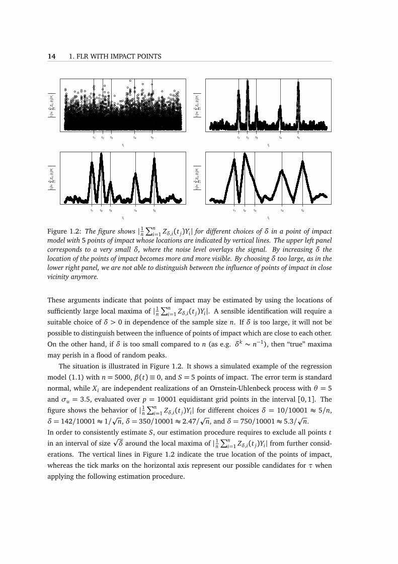
Figure 1.2: The figure shows | 1n∑n
i=1 Zδ,i(t j)Yi| for different choices of δ in a point of impactmodel with 5 points of impact whose locations are indicated by vertical lines. The upper left panelcorresponds to a very small δ, where the noise level overlays the signal. By increasing δ thelocation of the points of impact becomes more and more visible. By choosing δ too large, as in thelower right panel, we are not able to distinguish between the influence of points of impact in closevicinity anymore.
These arguments indicate that points of impact may be estimated by using the locations of
sufficiently large local maxima of | 1n∑n
i=1 Zδ,i(t j)Yi|. A sensible identification will require a
suitable choice of δ > 0 in dependence of the sample size n. If δ is too large, it will not be
possible to distinguish between the influence of points of impact which are close to each other.
On the other hand, if δ is too small compared to n (as e.g. δk ∼ n−1), then “true” maxima
may perish in a flood of random peaks.
The situation is illustrated in Figure 1.2. It shows a simulated example of the regression
model (1.1) with n = 5000, β(t) ≡ 0, and S = 5 points of impact. The error term is standard
normal, while X i are independent realizations of an Ornstein-Uhlenbeck process with θ = 5
and σu = 3.5, evaluated over p = 10001 equidistant grid points in the interval [0, 1]. The
figure shows the behavior of | 1n∑n
i=1 Zδ,i(t j)Yi| for different choices δ = 10/10001 ≈ 5/n,
δ = 142/10001≈ 1/p
n, δ = 350/10001≈ 2.47/p
n, and δ = 750/10001≈ 5.3/p
n.
In order to consistently estimate S, our estimation procedure requires to exclude all points t
in an interval of sizepδ around the local maxima of | 1n
∑ni=1 Zδ,i(t j)Yi| from further consid-
erations. The vertical lines in Figure 1.2 indicate the true location of the points of impact,
whereas the tick marks on the horizontal axis represent our possible candidates for τ when
applying the following estimation procedure.

1.4. ESTIMATING POINTS OF IMPACT 15
Estimation procedure:
Choose some δ > 0 such that there exists some kδ ∈ N with 1≤ kδ <p−1
2 and δ = kδ(b−a)/(p− 1). In a first step determine for all j ∈ J0,δ := kδ + 1, . . . , p− kδ
Zδ,i(t j) := X i(t j)−12(X i(t j −δ) + X i(t j +δ)).
Iterate for l = 1, 2,3, . . . :
• Determine
jl = ar g maxj∈Jl−1,δ
|1n
n∑
i=1
Zδ,i(t j)Yi|
and set bτl := t jl .
• Set Jl,δ := j ∈ Jl−1,δ| |t j − bτl | ≥pδ/2, i.e eliminate all points in an interval of size
pδ around bτl . Stop iteration if Jl,δ = ;.
Choose a suitable cut-off parameter λ > 0.
• Estimate S by
bS = ar g minl=0,1,2,...
|1n
∑ni=1 Zδ,i(bτl+1)Yi
( 1n
∑ni=1 Zδ,i(bτl+1)2)1/2
|< λ.
• bτ1, . . . , bτbS then are the final estimates of the points of impact.
A theoretical justification for this estimation procedure is given by Theorem 1.4. Its proof
along with the proofs of Proposition 1.1 and 1.2 below can be found in the Supplementary
Appendix C. Theory relies on an asymptotics n→∞ with p ≡ pn ≥ Ln1/κ for some constant
0< L <∞. It is based on the following additional assumption on the structure of X and Y .
Assumption 1.2.
a) X1, . . . , Xn are i.i.d. random functions distributed according to X . The process X is Gaussian
with covariance function σ(t, s).
b) The error terms ε1, . . . ,εn are i.i.d N(0,σ2) r.v. which are independent of X i .
Theorem 1.4. Under our setup and Assumptions 1.1 as well as 1.2 let δ ≡ δn → 0 as n→∞such that nδκ
| logδ| →∞ as well as δκ
n−κ+1 → 0. As n→∞ we then obtain
maxr=1,...,bS
mins=1,...,S
|bτr −τs| = OP(n− 1
k ). (1.11)

16 1. FLR WITH IMPACT POINTS
Additionally assume that δ2 = O(n−1) and that the algorithm is applied with cut-off parameter
λ≡ λn = A
√
√Var(Yi)n
log(b− aδ), where A>
p2.
Then
P(bS = S) → 1 as n→∞. (1.12)
The theorem of course implies that the rates of convergence of the estimated points of
impact depend on κ. If κ = 1, as e.g. for the Brownian motion or the Ornstein-Uhlenbeck
process, then maxr=1,...,bS mins=1,...,S |bτr − τs| = OP(n−1). Arbitrarily fast rates of convergence
can be achieved for very non-smooth processes with κ 1.
A suitable choice of δ satisfying the requirements of the theorem for all possible κ < 2 is
δ = Cn−1/2 for some constant C .
Recall that for l > 1, our algorithm requires that bτl is determined only from those points
t j wich are not inpδ/2-neighborhoods of any previously selected bτ1, . . . , bτl−1. This implies
that for any δ the number Mδ of iteration steps is finite, and Mδ = O( b−apδ/2) is the maximal
possible number of “candidate” impact points which can be detected for a fixed n and δ ≡ δn.
The size of these intervals is due to the use of the cut-off criterion for estimating S. It can easily
be seen from the proof of the theorem that in order to establish (1.11) it suffices to eliminate
all points in δ| logδ| neighborhoods of bτ1, . . . , bτl−1 which is a much weaker restriction.
We also want to emphasize that the cut-off value provided by the theorem heavily relies on
the Gaussian assumption. A different approach that may work under more general conditions
is to consider all selected local maxima bτ1, . . . , bτMδ and to estimate S by usual model selection
criteria like BIC.
This is quite easily done if it can additionally be assumed that, in model (1.1), β(t) = 0
for all t ∈ [a, b]. One may then apply a best subset selection by regressing Yi on all possible
subsets of X i(bτ1), . . . , X i(bτMδ), and by calculating the residual sum of squares RSSs for each
subset of size s. An estimate bS is obtained by minimizing
BICs = n log (RSSs/n) + s log (n) (1.13)
over all possible values of s.
If∫ b
a β(t)X i(t)d t 6= 0 this approach will of course lead to biased results, since part of the
influence of this component on the response variable Yi may be approximated by adding addi-
tional artificial “points of impact”. But an obvious idea is then to incorporate estimates of the
linear functional by relying on functional principal components. Recall the Karhunen-Loève
decomposition already discussed in Section 2, and note that∫ b
a β(t)X i(t)d t =∑∞
r=1αr⟨X ,ψr⟩with αr = ⟨ψr ,β⟩. For k, S ∈ N, estimates Òψr of ψr and a subset τ1, . . . , τS ∈ bτ1, . . . , bτMδ

1.4. ESTIMATING POINTS OF IMPACT 17
one may consider an approximate relationship which resembles an “augmented model” as
proposed by Kneip and Sarda (2011) in a different context:
Yi ≈k∑
r=1
αr⟨X i , Òψr⟩+S∑
r=1
βr X i(τr) + ε∗i . (1.14)
Based on corresponding least-squares estimates of the coefficients αr and βr , the number S
and an optimal value of k may then be estimated by the BIC criterion.
This approach also offers a way to select a sensible value of δ = Cn−1/2 for a suitable range
of values C ∈ [Cmin, Cmax]. For finite n, different choices of C (and δ) may of course lead to
different candidate values bτr , r = 1, 2, . . . . A straightforward approach is then to choose the
value of δ, where the respective estimates of impact points lead to the best fitting augmented
model (1.14). In addition to estimating S and an optimal value of k, BIC may thus also be
used to approximate an optimal value of C (and δ).
Recall that the above approach is applicable if Assumption 1.1 holds for some κ < 2. In a
practical application one may thus want to check the applicability of the theory by estimating
the value of κ from the data. We have E(Zδ,i(t j)2) = δκ
2c(t j)−2κ2 c(t j)
+ o(δκ) (see (1.26)
in the proof of Theorem 1.3). Consequently,E(Zδ,i(t j)2)E(Zδ/2,i(t j)2)
= 2κ + o(1) as δ → 0. Without
restriction assume that kδ is an even number. The above arguments motivate the estimator
bκ= log2
1p−2kδ
∑
j∈J0,δ
∑ni=1 Zδ,i(t j)2
1p−2kδ
∑
j∈J0,δ
∑ni=1 Zδ/2,i(t j)2
!
of κ. In Proposition 1.1 below it is shown that bκ is a consistent estimator of κ as n → ∞,
δ → 0. In practice, an estimate bκ 2 will indicate a process whose covariance function
possesses a non-smooth diagonal.
Proposition 1.1. Under the conditions of Theorem 1.4 we have
bκ= κ+OP(n−1/2 +δmin2,2/κ). (1.15)
A final theoretical result concerns the distance between X i(bτr) and X i(τr). It will be of cru-
cial importance in the next section on parameter estimation. Without restriction we will in the
following assume that points of impact are ordered in such a way that τr = ar g mins=1,...,S |bτr−τs|, r = 1, . . . , S.

18 1. FLR WITH IMPACT POINTS
Proposition 1.2. Under the assumptions of Theorem 1.4 we obtain for every r = 1, . . . , S
1n
n∑
i=1
(X i(τr)− X i(bτr))2 = Op(n
−1), (1.16)
1n
n∑
i=1
(X i(τr)− X i(bτr))εi = Op(n−1). (1.17)
1.5 Parameter estimates
Recall that Assumption 1.1 is only a sufficient, not a necessary condition of identifiability. Even
if this assumption is violated and the covariance functionσ(t, s) is very smooth, there may exist
alternative procedures leading to sensible estimators bτr . In the following we will thus only
assume that the points of impacts are estimated by some procedure such that P(bS = S)→ 1
as n → ∞ and such that (1.16) as well as (1.17) hold for all r = 1, . . . , S. Note that this
assumption is trivially satisfied if analysis is based on pre-specified points of impact as discussed
in the introduction.
In situations where it can be assumed that∫ b
a β(t)X i(t)d t = 0 a.s., we encounter Yi =∑S
r=1 βr X i(τr)+εi , i = 1, . . . , n, and the regression coefficient may be obtained by least squares
when replacing the unknown points of impact τr by their estimates bτr . More precisely, in this
case an estimator bβ = (bβ1, . . . , bβbS)
T of β = (β1, . . . ,βS)T is determined by minimizing
1n
n∑
i=1
(Yi −bS∑
r=1
br X i(bτr))2 (1.18)
over all possible values b1, . . . , bbS .
Let Xi(τ) := (X i(τ1), . . . , X i(τS))T , and let Στ := E(Xi(τ)Xi(τ)T ). Note that identifiability
of the regression model as stated in Theorem 1.1 in particular implies that Στ is invertible.
If bS = S, then by (1.16) and (1.17) the differences between bτr and τr , r = 1, . . . , S are
asymptotically negligible, and the asymptotic distribution of bβ coincides with the asymptotic
distribution the least squares estimator to be obtained if points of impact were known:
pn(bβ −β)→D N(0,σ2Σ−1
τ ) (1.19)
as n→∞. A proof is straightforward and thus omitted.
In the general case with β(t) 6= 0 for some t, we propose to rely on the augmented model
(1.14). Thus let bλ1 ≥ bλ2 ≥ . . . and Òψ1, Òψ2, . . . denote eigenvalues and eigenfunctions of the
empirical covariance operator of X1, . . . , Xn. Given estimates bτ1, . . . , bτbS and a suitable cut-off

1.5. PARAMETER ESTIMATES 19
parameter k estimates bβ = (bβ1, . . . , bβbS)
T of β = (β1, . . . ,βS)T and bα1, . . . , bαk of α1, . . . ,αk are
determined by minimizing
n∑
i=1
Yi −k∑
r=1
ar⟨X i , Òψr⟩ −bS∑
r=1
br X i(bτr)
!2
(1.20)
over all ar , bs, r = 1, . . . , k, s = 1, . . . , bS. Based on the estimated coefficients bα1, . . . , bαk, and
estimator of the slope function β is then given by bβ(t) :=∑k
r=1 bαkÒψr(t).
In the following we will rely on a slight change of notation in the sense that Yi , X i (and
εi) are centered data obtained for each case by subtracting sample means. As pointed out
in the remark, we argue that theoretical results stated in Section 4 remain unchanged for
this situation. In the context of (1.20) centering ensures that X i , i = 1, . . . , n, can be exactly
represented by X i =∑n
j=1⟨X i , Òψr⟩Òψr (necessarily bλ j = 0 for j > n).
Our theoretical analysis of the estimators defined by (1.20) relies on the work of Hall and
Horowitz (2007) who derive rates of convergence of the estimator bβ(t) in a standard func-
tional regression model with S = 0. Under our Assumption 1.2 their results are additionally
based on the following assumption on the eigendecompositions of X and β:
Assumption 1.3.
a) There exist some µ > 1 and some σ2 < C0 <∞ such that λ j − λ j+1 ≥ C−10 j−µ−1 for all
j ≥ 1.
b) β(t) =∑∞
j=1α jψ(t) for all t, and |α j| ≤ C0 j−ν for some ν > 1+ 12µ.
Hall and Horowitz (2007) show that if S = 0 and k = O(n1/(µ+2ν)), then∫ b
a (bβ(t) −
β(t))2d t = Op(n−(2ν−1)/(µ+2ν)). This is known to be an optimal rate of convergence under
the standard model.
When dealing with points of impact, some additional conditions are required. Note that
σ(t, s) =∑∞
j=1λ jψ j(t)ψ j(s). Let σ[k](t, s) :=∑∞
j=k+1λ jψ j(t)ψ j(s), and let Mk denote the
S× S matrix with elements σ[k](τr ,τs), r, s = 1, . . . , S. Furthermore, let λmin(Mk) denote the
smallest eigenvalue of the matrix Mk.
Assumption 1.4.
a) supt sup jψ j(t)2 ≤ Cψ for some Cψ <∞.
b) There exists some 0< C1 <∞ such that λ j ≤ C1 j−µ for all j.
c) There exists some 0< D <∞ such that λmin(Mk)≥ Dk−µ+1 for all k.
Condition a) is, for example, satisfied ifψ1,ψ2, . . . correspond to a Fourier-type basis. Note
that Assumption 1.3 a) already implies that λ j must not be less than a constant multiple of j−µ,

20 1. FLR WITH IMPACT POINTS
and thus Condition b) requires that j−µ is also an upper bound for the rate of convergence of
λ j . This in turn implies that∑∞
j=k+1λ j ≤ C2k−µ+1 as well as |σ[k](t, s)| ≤ C2C2ψ
k−µ+1 for some
C2 <∞ and all k. Condition c) therefore only introduces an additional regularity condition
on the matrix Mk. For the Brownian motion discussed in Section 3 it is easily seen that these
requirements are necessarily fulfilled with µ= 2.
We now obtain the following theorem:
Theorem 1.5. Under our setup and Assumptions 1.2 - 1.4 suppose that bS = S and that estimators
bτr satisfy (1.16) as well as (1.17) for all r = 1, . . . , S. If additionally k = O(n1/(µ+2ν)) and
n1/(µ+2ν) = O(k) as n→∞, then
‖bβ −β‖22 = Op(n−2ν/(µ+2ν)), (1.21)
∫ b
a(bβ(t)− β(t))2d t = Op(n
−(2ν−1)/(µ+2ν)). (1.22)
In the presence of points of impact the slope function β(t) can thus be estimated with
the same rate of convergence as in the standard model with S = 0. The estimators bβr of βr ,
r = 1, . . . , S, achieve a slightly faster rate of convergence.
1.6 Simulation study
We proceed by studying the finite sample performance of our estimation procedure described
in the preceding sections. For different values of n, p, observations (X i , Yi) are generated
according to the points of impact model (1.1) where εi ∼ N(0, 1) are independent error terms.
The algorithms are implemented in R, and all tables are based on 1,000 repetitions of the
simulation experiments. The corresponding R-code can be obtained from the authors upon
request.
The data X1, . . . , Xn are generated as independent Ornstein-Uhlenbeck processes (κ = 1)
with parameters θ = 5 and σu = 3.5 at p equidistant grid points over the interval [0,1]. Sim-
ulated trajectories are determined by using exact updating formulas as proposed by Gillespie
(1996). The simulation study is based on S = 2 points of impact located at τ1 = 0.25 and
τ2 = 0.75 with corresponding coefficients β1 = 2 as well as β2 = 1. Results are reported in
Table 1.1, where the upper part of the table refers to the situation with β(t) ≡ 0, while the
lower part represents a model with β(t) = 3.5t3 − 5.5t2 + 3t + 0.5.
In both cases, estimation of the points of impact relies on setting δ = C 1pn for C = 1, but
similar results could be obtained for a wide range of values C . The results are then obtained
1.6. SIMULATION STUDY 21
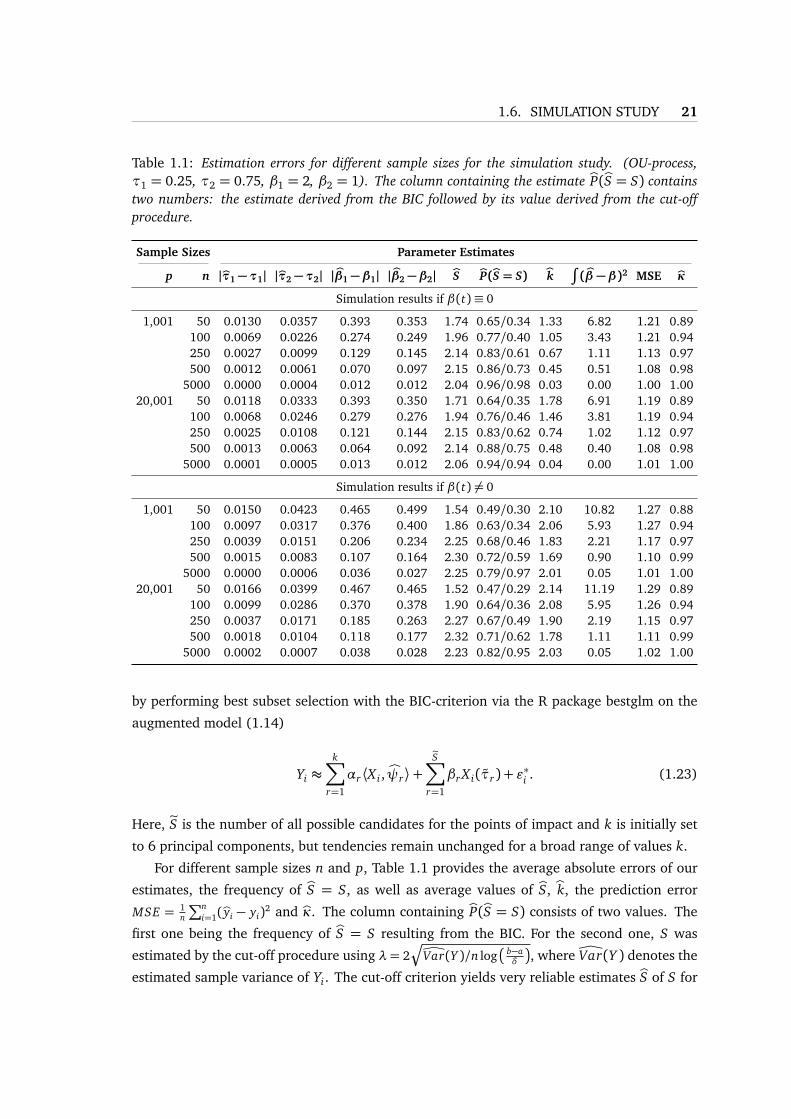
Table 1.1: Estimation errors for different sample sizes for the simulation study. (OU-process,τ1 = 0.25, τ2 = 0.75, β1 = 2, β2 = 1). The column containing the estimate bP(bS = S) containstwo numbers: the estimate derived from the BIC followed by its value derived from the cut-offprocedure.
Sample Sizes Parameter Estimates
p n |bτ1 − τ1| |bτ2 − τ2| | bβ1 −β1| | bβ2 −β2| bS bP(bS = S) bk∫( bβ −β)2 MSE bκ
Simulation results if β(t)≡ 0
1,001 50 0.0130 0.0357 0.393 0.353 1.74 0.65/0.34 1.33 6.82 1.21 0.89100 0.0069 0.0226 0.274 0.249 1.96 0.77/0.40 1.05 3.43 1.21 0.94250 0.0027 0.0099 0.129 0.145 2.14 0.83/0.61 0.67 1.11 1.13 0.97500 0.0012 0.0061 0.070 0.097 2.15 0.86/0.73 0.45 0.51 1.08 0.98
5000 0.0000 0.0004 0.012 0.012 2.04 0.96/0.98 0.03 0.00 1.00 1.0020,001 50 0.0118 0.0333 0.393 0.350 1.71 0.64/0.35 1.78 6.91 1.19 0.89
100 0.0068 0.0246 0.279 0.276 1.94 0.76/0.46 1.46 3.81 1.19 0.94250 0.0025 0.0108 0.121 0.144 2.15 0.83/0.62 0.74 1.02 1.12 0.97500 0.0013 0.0063 0.064 0.092 2.14 0.88/0.75 0.48 0.40 1.08 0.98
5000 0.0001 0.0005 0.013 0.012 2.06 0.94/0.94 0.04 0.00 1.01 1.00
Simulation results if β(t) 6= 0
1,001 50 0.0150 0.0423 0.465 0.499 1.54 0.49/0.30 2.10 10.82 1.27 0.88100 0.0097 0.0317 0.376 0.400 1.86 0.63/0.34 2.06 5.93 1.27 0.94250 0.0039 0.0151 0.206 0.234 2.25 0.68/0.46 1.83 2.21 1.17 0.97500 0.0015 0.0083 0.107 0.164 2.30 0.72/0.59 1.69 0.90 1.10 0.99
5000 0.0000 0.0006 0.036 0.027 2.25 0.79/0.97 2.01 0.05 1.01 1.0020,001 50 0.0166 0.0399 0.467 0.465 1.52 0.47/0.29 2.14 11.19 1.29 0.89
100 0.0099 0.0286 0.370 0.378 1.90 0.64/0.36 2.08 5.95 1.26 0.94250 0.0037 0.0171 0.185 0.263 2.27 0.67/0.49 1.90 2.19 1.15 0.97500 0.0018 0.0104 0.118 0.177 2.32 0.71/0.62 1.78 1.11 1.11 0.99
5000 0.0002 0.0007 0.038 0.028 2.23 0.82/0.95 2.03 0.05 1.02 1.00
by performing best subset selection with the BIC-criterion via the R package bestglm on the
augmented model (1.14)
Yi ≈k∑
r=1
αr⟨X i , Òψr⟩+eS∑
r=1
βr X i(τr) + ε∗i . (1.23)
Here, eS is the number of all possible candidates for the points of impact and k is initially set
to 6 principal components, but tendencies remain unchanged for a broad range of values k.
For different sample sizes n and p, Table 1.1 provides the average absolute errors of our
estimates, the frequency of bS = S, as well as average values of bS, bk, the prediction error
MSE = 1n
∑ni=1(byi − yi)2 and bκ. The column containing bP(bS = S) consists of two values. The
first one being the frequency of bS = S resulting from the BIC. For the second one, S was
estimated by the cut-off procedure using λ= 2Ç
ÔVar(Y )/n log
b−aδ
, where ÔVar(Y ) denotes the
estimated sample variance of Yi . The cut-off criterion yields very reliable estimates bS of S for

22 1. FLR WITH IMPACT POINTS
n = 5, 000, but showed a clear tendency to underestimate S for smaller sample sizes. The
BIC-criterion however proves to possess a much superior behavior in this regards for small n
but is outperformed by the cut-off criterion for n= 5, 000 in the case β(t) 6= 0.
In order to match bτss=1,...,bS and τrr=1,2 the interval [0,1] is partitioned into I1 =
0, 12 (τ1 +τ2)
and I2 =
12 (τ1 +τ2), 1
. The estimate bτs in interval Ir with the minimal dis-
tance to τr is then used as an estimate for τr . No point of impact candidate in Interval Ir
results in an ”unmatched” τr , r = 1, . . . , S and a missing value when computing averages.
The table shows that estimates of points of impact are generally quite accurate even for
smaller sample sizes. The error decreases rapidly as n increases, and this improvement is
essentially independent of p. As expected, since β2 < β1, the error of the absolute distance
between the second point of impact and its estimate is larger than the error for the first point
of impact.
Moreover, due to the common effect of the trajectory X i(·) on Yi , the overall estimation
error in the case where β(t) 6= 0 is slightly higher than in the first case. At a first glance one
may be puzzled by the fact that for n = 5, 000 and p = 1,001 the average error |bτr − τr | is
considerably smaller than the distance 1p−1 =
11000 between two adjacent grid points. But note
that our simulation design implies that τr ∈ t j| j = 1, . . . , p, r = 1, . . . , S, for p = 1,001 as
well as p = 20, 001. For medium to large sample sizes there is thus a fairly high probability
that bτr = τr . The case p = 1,001 particularly profits from this situation. Finally it can be seen
that estimates for bκ tend to slightly underestimate the true value κ= 1 for small values of n.
1.7 Application to real data
In this section the algorithm from Section 4 is applied to a dataset consisting of Canadian
weather data. In this dataset we relate the mean relative humidity to hourly temperature data.
In the Supplementary Appendix A a further application can be found. We there analyze spectral
data which play an important role in spectrophotometry and different applied scientific fields.
In both examples the algorithm is applied to centered observations and the estimation
procedure from Section 4 is modified by eliminating all points in an interval of size δ| logδ|around a point of impact candidate bτ j , which is still sufficient to establish assertion (1.11).
After estimating eS possible candidates for the points of impact, the approximate model
(1.14),
Yi ≈k∑
r=1
αr⟨X i , Òψr⟩+eS∑
r=1
βr X i(τr) + ε∗i ,
is used, where initially k = 6 is chosen. Over a fine grid of different values of δ, points of
impact and principal components are selected simultaneously by best subset selection with
the BIC-criterion and the model corresponding to the minimal BIC is then chosen. The max-

1.7. APPLICATION TO REAL DATA 23
0.0 0.2 0.4 0.6 0.8 1.0
tem
pera
ture
Tem
pera
ture
0.2 0.3 0.4 0.5 0.6 0.7 0.8
CO
R
1n
∑ i=1n
Zδ, i(t
j)Yi
Figure 1.3: The upper panel of this figure shows a trajectory from the observed temperature curvesof the Canadian weather data. The lower panel shows | 1n
∑ni=1 Zδ,i(t j)Yi| during the selection
procedure. Locations of selected points of impact in the augmented model are indicated by greylines. The location of the remaining candidate is displayed by a black line.
imum number of variables selected by the BIC-criterion is set to 6 and all curves have been
transformed to be observed over [0,1] when applying the algorithm from Section 4. The
performance of the model is then measured by means of a cross-validated prediction error.
In the Canadian weather dataset, the hourly mean temperature and relative humidity from
the 15 closest weather stations in an area around 100 km from Montreal was obtained for each
of the 31 days in December 2013. The data was compiled from http://climate.weather.gc.ca. Weather stations with more than ten missing observations on the temperature or rela-
tive humidity were discarded from the dataset. The remaining stations had their non available
observations replaced by the mean of their closest observed predecessor and successor. After
preprocessing a total of n = 13 weather stations remained and for each station p = 744
equidistant hourly observations of the temperature were observed. The response variable Yi
was taken to be the mean over all observed values of the relatively humidity at station i.
A cross-validated prediction error was calculated for three competing regression models
based on (1.14). In the first model, the mean relative humidity for each station was explained
by using the approximate model which combines the points of impacts with a functional part.
The second and third model describe the cases k = 0 and eS = 0 in the approximate model,
consisting only of points of impact and the functional part respectively. For the first two models,
points of impact were determined by considering a total of 146 equidistant values of δ between
0.10 and 0.49. In all models BIC was used to approximate the optimal values of the respective

24 1. FLR WITH IMPACT POINTS
Table 1.2: Estimated number of principal components k, points of impact S, prediction error andthe median of (yi − byi)2 for the Canadian weather data.
Model bk bS MSPE median((y − y)2)
Augmented 3 3 2.314 0.251Points of impact 0 3 1.714 0.974FLR 6 0 5.346 1.269
tuning parameters δ, S, and/or k in a first step. The mean squared prediction error MSPE =1n
∑ni=1(yi − byi)2 was then calculated by means of a leave one out cross-validation based on
the chosen points of impact and/or principal components from the first step. Additionally,
the median of (yi − byi)2, i = 1, . . . , n, has been calculated as a more robust measure of the
error. Depicted in the upper panel of Figure 1.3 is the observed temperature trajectory for the
weather station “McTavish”, showing a rather rough process. The lower panel of this figure
show | 1nn∑
i=1Zδ,i(t j)Yi | for the optimal value of δ = 0.18 as obtained by the best model fit of
the approximate model. While orange lines represent the locations of the points of impact
which were actually selected with the help of the BIC-criterion, the location of the remaining
candidates are indicated by black vertical lines.
Table 1.2 provides the empirical results when fitting the three competing models. In terms
of the prediction error it can clearly be seen from the table that the frequently applied func-
tional linear regression model is outperformed by the model consisting solely of points of
impact as well as the augmented (approximate) model. This impression is supported by the
last column of the table which gives the median value of (yi − byi)2, showing additionally that,
typically, the augmented model performs even better than the plain points of impact model.
An estimate bκ= 0.14 for κwas obtained for δ ≈ 0.3, i.e. the midpoint of the chosen values
of δ. The estimated value of κ = 0.14 corresponds to rather rough sample paths as shown in
the upper plot of Figure 1.3.
In view of the small sample size results have to be interpreted with care, and we therefore
do not claim that this application provides important substantial insights. Its main purpose
is to serve as illustration for classes of problems where our approach may be of potential
importance. It clearly shows that some relevant processes observed in practice are non-smooth.
With contemporary technical tools temperatures can be measured very accurately, leading to
a negligible measurement error. But temperatures, especially in Canada, can vary rapidly over
time. The rough sample paths thus must be interpreted as an intrinsic feature of temperature
processes and cannot be explained by any type of “error”.

1.8. PROOFS OF SOME THEOREMS 25
1.8 Proofs of some theorems
Proof of Theorem 1.1. Set βr := 0 for r = S + 1, . . . , S∗, and consider an arbitrary j ∈1, . . . , S∗. Choose 0< ε <minr,s∈1,...,S∗,r 6=s |τr−τs| small enough such that conditions i)-iv)of Definition 1 are satisfied. Using (1.2) we obtain a decomposition into two uncorrelatedcomponents Xε,τ j
(·) and ζε,τ j(X ) fε,τ j
(·):
E
∫ b
a
(β(t)− β∗(t))X (t)d t +S∗∑
r=1
(βr − β∗r )X (τr)2
= E
∫ b
a
(β(t)− β∗(t))Xε,τ j(t)d t +
S∗∑
r=1
(βr − β∗r )Xε,τ j(τr)
2
+E
∫ b
a
(β(t)− β∗(t))ζε,τ j(X ) fε,τ j
(t)d t +S∗∑
r=1
(βr − β∗r )ζε,τ j(X ) fε,τ j
(τr)2
≥E
∫ b
a
(β(t)− β∗(t))ζε,τ j(X ) fε,τ j
(t)d t
+∑
r 6= j
(βr − β∗r )ζε,τ j(X ) fε,τ j
(τr) + (β j − β∗j )ζε,τ j(X ) fε,τ j
(τ j)2
≥ 2var(ζε,τ j(X ))(β j − β∗j ) fε,τ j
(τ j)
∫ b
a
(β(t)− β∗(t)) fε,τ j(t)d t +
∑
r 6= j
(βr − β∗r ) fε,τ j(τr)
!
+ var(ζε,τ j(X ))(β j − β∗j )
2 fε,τ j(τ j)
2.
By condition iv) we have
|∑
r 6= j
(βr − β∗r ) fε,τ j(τr)| ≤ εS∗max
r 6= j|βr − β∗r || fε,τ j
(τ j)|,
while boundedness of β(·) and β∗(·) implies that there exits a constant 0≤ D <∞ such thatfor all sufficiently small ε > 0
|∫ b
a
(β(t)− β∗(t)) fε,τ j(t)d t| ≤ ε
∫
[a,b]\[τ j−ε,τ j+ε]D| fε,τ j
(τ j)|d t +
∫ τ j+ε
τ j−ε(1+ ε)D| fε,τ j
(τ j)|d t
≤ ε(b− a+ 2(1+ ε))D| fε,τ j(τ j)|.
When combining these inequalities we can conclude that for all sufficiently small ε we have
E(∫ b
a (β(t)−β∗(t))X (t)d t +
∑S∗
r=1(βr −β∗r )X (τr))2 > 0 if β j −β∗j 6= 0. Since j ∈ 1, . . . , S∗ is
arbitrary, the assertion of the theorem is an immediate consequence.

26 1. FLR WITH IMPACT POINTS
Proof of Theorem 1.2. Choose some arbitrary t ∈ (a, b) and some 0< ε < 1 with ε≤ εt . Byassumption there exists a k ∈ N as well as some f ∈ C (t,ε, [a, b]) such that |⟨ f ,ψr⟩| > 0 forsome r ∈ 1, . . . , k and sups∈[a,b] | fk(s)− f (s)| ≤ ε/3, where fk(s) =
∑kr=1⟨ f ,ψr⟩ψr(s). The
definition of C (t,ε, [a, b]) then implies that fk(t)≥ 1− ε/3 as well as
sups∈[a,b]
| fk(s)| ≤ 1+ε
3≤ (1+ ε)(1−
ε
3)≤ (1+ ε) fk(t),
sups∈[a,b],s 6∈[t−ε,t+ε]
| fk(s)| ≤ε
3≤ ε(1−
ε
3)≤ ε fk(t). (1.24)
Now define the functional ζε,t by ζε,t(X ) :=∑k
r=1⟨ f ,ψr ⟩λr⟨X ,ψr⟩. Recall that the coefficients
⟨X ,ψr⟩ are uncorrelated and var(⟨X ,ψr⟩) = λr . By (1.5) we obtain
fε,t(s) :=E(X (s)ζε,t(X ))var(ζε,t(X ))
=
E
(∞∑
j=1⟨X ,ψ j⟩ψ j(s))(
∑kr=1
⟨ f ,ψr ⟩λr⟨X ,ψr⟩)
var(ζε,t(X ))
=
∑kr=1⟨ f ,ψr⟩ψr(s)
var(ζε,t(X ))=
fk(s)var(ζε,t(X ))
.
Furthermore, var(ζε,t(X )) =∑k
r=1⟨ f ,ψr ⟩2λr
> 0, and it thus follows from (1.24) that the func-
tional ζ(t, X ) satisfies conditions i) - iv) of Definition 1. Since t ∈ (a, b) and ε are arbitrary, X
thus possesses specific local variation.
Proof of Theorem 1.3. First note that Assumption 1.1 implies that the absolute values of all
first and second order partial derivatives ofω(t, s, z) are uniformly bounded by some constant
M <∞ for all (t, s, z) in the compact subset [a, b]2 × [0, b− a] of Ω.
By definition of Zδ it thus follows from a Taylor expansion of ω that for t ∈ (a, b), any suffi-
ciently small δ > 0 and some constant M1 <∞
E(X (t)Zδ(X , t)) = σ(t, t)−12σ(t, t −δ)−
12σ(t, t +δ)
= ω(t, t, 0)−12ω(t, t −δ,δκ)−
12ω(t, t +δ,δκ)
= δκc(t) + R1;δ,t , with supt∈[a+δ,b−δ]
|R1;δ,t | ≤ M1δmin2κ,2. (1.25)
For the variance of Zδ(X , t) we obtain by similar arguments
var(Zδ(X , t)) = 2ω(t, t, 0)−ω(t, t −δ,δκ)−ω(t, t +δ,δκ)−12(ω(t, t, 0)−ω(t +δ, t −δ, (2δ)κ))
−14(2ω(t, t, 0)−ω(t −δ, t −δ, 0)−ω(t +δ, t +δ, 0))
= δκ
2c(t)−2κ
2c(t)
+ R2;δ,t , with supt∈[a+δ,b−δ]
|R2;δ,t |< M2δmin2κ,2 (1.26)

1.8. PROOFS OF SOME THEOREMS 27
for some constant M2 <∞. Moreover, for any 0 < c <∞ Taylor expansions of ω yield thatfor any sufficiently small δ > 0 and all u ∈ [−c, c]
E(X (t + uδ)Zδ(X , t)) = σ(t + uδ, t)−12σ(t + uδ, t −δ)−
12σ(t + uδ, t +δ)
= ω(t, t, 0)−12ω(t, t −δ,δκ)−
12ω(t, t +δ,δκ)
− c(t)δκ
|u|κ −12(|u+ 1|κ − 1)−
12(|u− 1|κ − 1)
+ R3;c,u,δ,t (1.27)
=− c(t)δκ
|u|κ −12|u+ 1|κ −
12|u− 1|κ
+ R4;c,u,δ,t , (1.28)
where for some constants M3,c <∞ and M4,c <∞
supt∈[a+δ,b−δ]
R3;c,u,δ,t ≤ M3,c(|u|1/2δ)min2κ,2, supt∈[a+δ,b−δ]
R4;c,u,δ,t ≤ M4,cδmin2κ,2
hold for all u ∈ [−c, c]. Finally, Assumption 1.1 implies that there exists a constant M5 <∞such that for all s ∈ [a, b] with |t − s| ≥ δ
|E(X (s)Zδ(X , t))|=|ω(s, t, |s− t|κ)−12ω(s, t −δ, |s− t +δ|κ)−
12ω(s, t +δ, |s− t −δ|κ)|
≤
(
M5δ2
|t−s|2−κ if κ 6= 1
M5δ2 if κ= 1.
(1.29)
It follows from (1.25), (1.28), and (1.29) that for arbitrary t ∈ (a, b) and any ε > 0 there
exist a δε > 0 as well as a constant aε ≥ 1 such that for all δ ≤ δε
|E(X (s)Zδ(X , t))| ≤ (1+ ε)E(X (t)Zδ(X , t)) for all s ∈ [a, b], s 6= t
|E(X (s)Zδ(X , t))| ≤ ε ·E(X (t)Zδ(X , t)) for all s ∈ [a, b], |s− t| ≥ aεδ.
Together with (1.26), the assertion of the theorem is an immediate consequence.
Proof of Theorem 1.5. Let bθi j := ⟨X i , Òψ j⟩, θi j := ⟨X i ,ψ j⟩, and α j := ⟨β , Òψ j⟩ for all i, j. Us-
ing empirical eigenfunctions we obtain X i =∑n
j=1bθi jÒψ j and
∫ ba β(t)X i(t)d t =
∑nj=1 α j
bθi j .
Therefore,
Yi =n∑
j=1
α j +S∑
r=1
βrÒψ j(τr)
bθi j + εi , (1.30)
and for all possible values b1, . . . , bS and all a1, . . . , ak
k∑
j=1
a jbθi j +
S∑
r=1
br X i(bτr) =k∑
j=1
a j +S∑
r=1
brÒψ j(bτr)
bθi j +n∑
j=k+1
S∑
r=1
brÒψ j(bτr)bθi j (1.31)

28 1. FLR WITH IMPACT POINTS
for all i = 1, . . . , n. By definition, bλ j =1n
∑ni=1
bθ2i j , j = 1, . . . , n, and for j 6= l the coefficients bθi j
and bθil are empirically uncorrelated, i.e.∑n
i=1bθi jbθil = 0. It follows that for any given values
b1, . . . , bS the values bα(b) j , j = 1, . . . , k, minimizing∑n
i=1
Yi −∑k
j=1 a jbθi j −
∑Sr=1 br X i(bτr)
2
over all a1, . . . , ak are given by
bα(b) j = α j + bλ−1j
1n
n∑
i=1
bθi jεi +S∑
r=1
(βrÒψ j(τr)− br
Òψ j(bτr)), j = 1, . . . , k. (1.32)
Note that α j + bλ−1j
1n
∑ni=1
bθi jεi is identical to the estimate of α j to be obtained in a standard
functional linear regression model with no points of impact. Theorem 1 of Hall and Horowitz
(2007) thus implies that
∫ b
a
β(t)−k∑
j=1
(α j + bλ−1j
1n
n∑
i=1
bθi jεi)Òψ j(t)d t
!2
d t = Op(n−(2ν−1)/(µ+2ν)). (1.33)
Further analysis requires to analyze the differences between θi j ,ψ j and their empirical coun-
terparts bθi j , Òψ j . By Assumptions 1.2 - 1.4 and k = O(n1/(µ+2ν)), Theorems 1 and 2 togetherwith equation (2.8) of Hall and Hosseini-Nasab (2006) imply that for any q = 1,2, 3, . . . thereexists some Aq, Bq <∞ such that
E
|λ j − bλ j |q
≤ Aqn−q/2, supt
E
|Òψ j(t)−ψ j(t)|
≤ Bqn−q/2 jq(µ+1), j = 1, . . . , k+ 1 (1.34)
for all sufficiently large n. Let X [k]i := X i −∑k
j=1bθi jÒψ j . Recall that λ j = O( j−µ) and note
that by Assumptions 1.3 and 1.4, n−1/2n2/(µ+2ν) = o(n(−µ+1)/(µ+2ν)), while n(−µ+1)/(µ+2ν) =
O(σ[k](τr ,τr)). By (1.34) we thus obtain for all t, s ∈ [a, b]
1n
n∑
i=1
X [k]i (t)X[k]i (s) =
1n
n∑
i=1
X i(t)X i(s)−k∑
j=1
bλ jÒψ j(t)Òψ j(s)
= σ(t, s)−k∑
j=1
λ jψ j(t)ψ j(s) +k∑
j=1
λ j(ψ j(t)ψ j(s)− Òψ j(t)Òψ j(s))
+k∑
j=1
(λ j − bλ j)Òψ j(t)Òψ j(s) +OP(n−1/2)
= σ[k](t, s) +OP(n−1/2n2/(µ+2ν)) = σ[k](t, s) + oP(n
(−µ+1)/(µ+2ν)).
(1.35)

1.8. PROOFS OF SOME THEOREMS 29
At the same time (1.16) leads to
1n
n∑
i=1
(X [k]i (τr)− X [k]i (bτr))2 =
1n
n∑
i=1
(X i(τr)− X i(bτr))2 −
k∑
j=1
bλ j(Òψ j(τr)− Òψ j(bτr))2
≤1n
n∑
i=1
(X i(τr)− X i(bτr))2 = OP(n
−1).
(1.36)
for all r = 1, . . . , S. Expressions (1.35) and (1.36) together imply that for all r, s
1n
n∑
i=1
X [k]i (bτr)X[k]i (bτs) = σ
[k](τr ,τs) + oP(n(−µ+1)/(µ+2ν)). (1.37)
Let X[k]i := (X [k]i (bτ1), . . . , X [k]i (bτS))T and note that by (1.37) we have 1n
∑ni=1 X[k]i (X
[k]i )
T =
Mk+ oP(n(−µ+1)/(µ+2ν)). By Assumption 1.4 b) we can conclude that with probability tending
to 1 as n→∞ the matrix 1n
∑ni=1 X[k]i (X
[k]i )
T is invertible,
n(−µ+1)/(µ+2ν)(1n
n∑
i=1
X[k]i (X[k]i )
T )−1 = n(−µ+1)/(µ+2ν)(Mk)−1 + oP(1) (1.38)
and hence by (1.30) - (1.32) the least squares estimator bβ of β can be written in the form
bβ = (1n
n∑
i=1
X[k]i (X[k]i )
T )−1 1n
n∑
i=1
X[k]i
S∑
r=1
βr X [k]i (τr) +n∑
j=k+1
α jbθi j + εi
!
. (1.39)
By (1.36) and (1.37) we obtain
1n
n∑
i=1
X[k]i
S∑
r=1
βr X [k]i (τr) =1n
n∑
i=1
X[k]i (X[k]i )
Tβ +OP(n(−µ+1)/2(µ+2ν) · n−1/2). (1.40)
The results of Hall and Horowitz (2007) imply that∑n
j=k+1 α2j = OP(n−(2ν−1)/(µ+2ν)). The
Cauchy-Schwarz inequality thus leads to
|1n
n∑
i=1
X [k]i (bτr)(n∑
j=k+1
α jbθi j)|= |
n∑
j=k+1
α jbλ jÒψ j(bτr)|
≤
√
√
√
√
n∑
j=k+1
bλ jα2j
√
√
√
√
n∑
j=k+1
bλ jÒψ j(bτr)2 ≤
√
√
√
√bλk+1
n∑
j=k+1
α2j
√
√
√1n
n∑
i=1
X [k]i (bτr)2
= OP(n−(µ+2ν−1)/2(µ+2ν) · n(−µ+1)/2(µ+2ν)) (1.41)

30 1. FLR WITH IMPACT POINTS
for all r = 1, . . . , S. Furthermore, Òψ j(t) = bλ−1j
1n
∑ni=1
bθi jX i(t), and hence the Cauchy-Schwarzinequality yields
|Òψ j(τr)− Òψ j(bτr)|= |bλ−1j
1n
n∑
i=1
bθi j(X i(τr)− X i(bτr))| ≤ bλ−1/2j
√
√
√1n
n∑
l=1
(X l(τr)− X l(bτr))2. (1.42)
Now note that by the independence of bθi j and εi we have bλ−1/2j
1n
∑ni=1
bθi jεi = OP(n−1/2). By(1.17) it therefore follows from (1.42) that
1n
n∑
i=1
(X [k]i (bτr)− X [k]i (τr))εi =1n
n∑
i=1
(X i(bτr)− X i(τr))εi −k∑
j=1
1n
n∑
i=1
bθi jεi(Òψ j(bτr)− Òψ j(τr))
= OP((k+ 1)n−1) = OP(n−(µ+2ν−1)/(µ+2ν)).
Using (1.35), it is immediately seen that 1n
∑ni=1 X [k]i (τr)εi = OP(n−1/2n(−µ+1)/2(µ+2ν)). Con-
sequently,
1n
n∑
i=1
X [k]i (bτr)εi =1n
n∑
i=1
X [k]i (τr)εi +1n
n∑
i=1
(X [k]i (bτr)− X [k]i (τr))εi = OP(n−1/2n(−µ+1)/2(µ+2ν)) (1.43)
By Assumption 1.4 c) we can infer from (1.38) that the maximal eigenvalue of the matrix( 1
n
∑ni=1 X[k]i (X
[k]i )
T )−1 can be bounded by λmax((1n
∑ni=1 X[k]i (X
[k]i )
T )−1) = OP(n(µ−1)/(µ+2ν)).It therefore follows from (1.39) - (1.43) that
bβ = β +OP(n(µ−1)/(µ+2ν) · n(−µ+1)/2(µ+2ν) · n−(µ+2ν−1)/2(µ+2ν))) = β +OP(n
−ν/(µ+2ν)).
This proves (1.21). Using (1.32), it follows that the least squares estimators bα j of α j are givenby
bα j = α j + bλ−1j
1n
n∑
i=1
bθi jεi +S∑
r=1
(βr − bβr)Òψ j(τr)−S∑
r=1
bβr(Òψ j(bτr)− Òψ j(τr)), j = 1, . . . , k (1.44)
But (1.34) and (1.21) imply that
k∑
j=1
(S∑
r=1
(βr − bβr)Òψ j(τr))2 = OP(kn−2ν/(µ+2ν)) = OP(n
−(2ν−1)/(µ+2ν)), (1.45)
while by (1.34) and (1.42)
k∑
j=1
(Òψ j(τr)− Òψ j(bτr))2 ≤
kλk
1n
n∑
i=1
(X i(τr)− X i(bτr))2 = OP(n
−(2ν−1)/(µ+2ν)),

1.8. PROOFS OF SOME THEOREMS 31
and therefore
k∑
j=1
(S∑
r=1
bβr(Òψ j(bτr)− Òψ j(τr)))2 = OP(n
−(2ν−1)/(µ+2ν)). (1.46)
Assertion (1.22) now is an immediate consequence of (1.33) and (1.44) - (1.46).


33
Supplement to: Functional Linear Regressionwith Points of Impact
This supplement to the chapter “Functional Linear Regression with Points of Impact”
contains three Appendices. An application to NIR data can be found in Appendix A. In
Appendix B it is shown that the eigenfunctions of a Brownian motion satisfy assertion 1.6
in Theorem 1.2. Appendix C provides the proofs of Theorem 1.4, Proposition 1.1 as well
as the proof of Proposition 1.2.
Appendix A Application to near infrared data
The estimation procedure is applied to a well known near infrared dataset from the Chambers-
burg Shoot-out 2002. This data consists of a series of NIR spectra of pharmaceutical tablets,
which is measured over p = 650 equidistant wavelengths ranging from 600− 1898 nm. The
data can for example be found in the R Package ChemometricsWithRData Wehrens (2011).
We focus on the first calibration dataset, consisting of n= 155 spectra.
The response variable Yi is chosen to be the weight of tablet i. All results for the augmented
and point of impact model are based on minimizing the BIC-criterion over a fine grid of 132
values of δ between 0.05 and 0.45 in a first step. The number k of principal components
for the functional linear regression model was estimated by using a 10-fold cross-validation
but conclusions remained unchanged using the BIC. Moreover, results from the augmented as
well as from the functional linear model remained stable even if we increased the maximum
number of the first principal components initially allowed to enter the model up to at least 10.
The observations corresponding to the frequency of 1820 inhabited an anomaly high vari-
ance and has for each curve been replaced by the mean of their closest neighbors. The replaced
point was mostly visible as an outlier in the “correlation” plots between Yi and Zδ,i(t) but did
not change the overall conclusions as given in Table A.1. A typical curve from the Shoot-out
dataset is shown in the upper panel of Figure A.1. It is common to NIR data that the observed

34 1. SUPPLEMENT TO: FLR WITH IMPACT POINTS
600 800 1000 1200 1400 1600 1800
1T
800 1000 1200 1400 1600
CO
R
1n
∑ i=1n
Zδ, i(t
j)Yi
Figure A.1: While the upper plot shows the trajectory of a typical data curve from the NIR data,the lower part of the figure show | 1n
∑ni=1 Zδ,i(t j)Yi| for the optimal value of δ as obtained by
the best model fit of the augmented model. Selected points of impact candidates are tagged grey,remaining candidates are indicated by black vertical lines.
curves are essentially smooth but show variability around some wavelengths and variability
increases towards the end of the measured wavelengths. Remember that the smoothness of
the observed sample paths is reflected by κ. In an idealized setting under Assumption 1 (Kneip
et al. 2013) one would expect bκ to be independent from the particular choice of δ. In practice
however covariance functions are often more complex as the smoothness of the observed pro-
cess can change over the observed sample points. The estimate bκ = 1.37 for κ was obtained
for the midpoint of the considered values of δ and supports the impression that the curves in
this example exhibit smoother sample paths when compared to the weather data. Figure A.1
also shows the “correlation” between Yi and Zδ,i(t) for the optimal value of δ being 0.176.
The two points of impact were estimated at wavelengths 1662 and 904. The mean squared
prediction error in the third column of Table A.1 was derived from a 10-fold cross-validation
after having chosen points of impact and/or principal components by our selection criteria in
a first step. The qualitative results derived from the MSPE are supported by the calculated
Table A.1: Estimated number of principal components k, points of impact S, prediction error andthe median of (yi − yi)2 for the NIR data.
Model bk bS MSPE median((y − y)2)
Augmented 0 2 1.487 0.329Points of impact 0 2 1.487 0.329FLR 3 0 1.616 0.428

B. APPROXIMATION PROPERTIES OF EIGENFUNCTIONS 35
values of the median value of (yi− yi)2 for each model given in the last column. In this exam-
ple, the augmented model was estimated identical to the model consisting solely of points of
impact and both models are slightly superior in terms of the prediction error when compared
to the traditional functional linear regression model while, at the same time, being easier to
be interpreted through their two points of impact.
Appendix B On the approximation properties of the eigenfunctions
of a Brownian motion
In this Appendix it is shown that the eigenfunctions of a Brownian motion satisfy assertion
(1.6) in Theorem 1.2.
For t ∈ (a, b) and ε > 0 let C (t,ε, [a, b]) denote the space of all continuous functions f ∈L2([a, b])with the properties that f (t) = sups∈[a,b] | f (s)|= 1 and f (s) = 0 for s 6∈ [t−ε, t+ε].
Theorem 1.2. Let ψ1,ψ2, . . . be a system of orthonormal eigenfunctions corresponding to the
non-zero eigenvalues of the covariance operator Γ of X . If for all t ∈ (a, b) there exists an εt > 0
such that
limk→∞
inff ∈C (t,ε,[a,b])
sups∈[a,b]
| f (s)−k∑
r=1
⟨ f ,ψr⟩ψr(s)|= 0 for every 0< ε < εt , (1.6)
then the process X possesses specific local variation.
We have to show the following statement:
Lemma B.1. Letφr(s) =p
2sin((r− 12)πs), r = 1,2, . . . , be the system of orthonormal eigenfunc-
tions derived from a Brownian motion on [0, 1]. Then φr(s), r = 1, 2, . . . satisfy assertion (1.6)
in Theorem 1.2.
Proof of Lemma B.1. Assertion (1.6) follows from elementary properties of Fourier series andsine functions. To see this, recall that the basis functions of a Fourier-Sine-Series to approxi-mate a function with periodicity P = 4 are given by Φn(s) = sin(1
2πns) for n = 1, 2, . . . . It isnow immediately clear, that the eigenfunctions φr(s) =
p2 sin((r − 1
2)πs), r = 1,2, . . . , areproportional to the functions of Φn(s), for n= 2r − 1, i.e. when n is uneven.Select an arbitrary 0< t < 1 and 0< ε≤ εt =min(t, 1− t). Let ft ∈ C (t,ε, [0, 1]) be defined

36 1. SUPPLEMENT TO: FLR WITH IMPACT POINTS
as ft(s) :=max(1− |s− t|/ε, 0), s ∈ [0,1]. This function can be easily extended on the wholereal line to an odd function Ft with periodicity P = 4 by
Ft(s) =
ft(s), s ∈ [0,1]
ft(2− s), s ∈ [1,2]
−Ft(4− s), s ∈ [2,4]
Ft(s− 4m), s ∈ [4m, 4(m+ 1)], m= 1, . . .
−Ft(s), s ≤ 0.
It is then known that the Fourier series of an odd periodic function reduces to a Fourier-Sine-
Series. Moreover, from well known results about Fourier series, we have that the Fourier series
of a continuous periodic function F , which is piecewise continuous differentiable, converges
uniformly to F .
The only question left is why we can discard the sine basis functions Φn(s) for n even. This
point is immediately seen if we look at Ft(s) for s ∈ [0,4] which is illustrated in Figure B.1 for
a specific value of t and ε.
0 1 2 3 4
Ft(
s)
−1
01
Figure B.1: The figure shows Ft(s) for t = 0.7 and ε = 0.2 over the interval [0,4]. Ft(s) is anodd function with periodicity 4. The function is point symmetric at s = 2 on [0, 4].
First note that all even sine basis functions Φn(s), n = 2,4, . . . , have periodicity 2. But
by construction Ft(s) is point symmetric at s = 2 and hence, for n = 2, 4,6, . . . , we have
⟨Ft ,Φn⟩ = 0, i.e. the coefficients of all even sine basis functions in the Fourier-Sine-Series are
0. Uniform convergence on [0, 1] to Ft(s) follows immediately for the system of the sine basis
functions Φn(s) for n even and hence for the system of the eigenfunctions φr . Since t and ε
were arbitrary, the system of eigenfunctions satisfy indeed assertion (1.6).

C. ADDITIONAL PROOFS 37
Appendix C Additional proofs
In this appendix Theorem 1.4 and Propositions 1.1 and 1.2 are proven. We begin by repeating
the two main assumptions and Theorem 1.4.
Assumption 1.1. For some open subset Ω ⊂ R3 with [a, b]2 × [0, b − a] ⊂ Ω, there exists a
twice continuously differentiable function ω : Ω→ R as well as some 0 < κ < 2 such that for all
t, s ∈ [a, b]
σ(t, s) =ω(t, s, |t − s|κ). (1.8)
Moreover,
0< inft∈[a,b]
c(t), where c(t) := −∂
∂ zω(t, t, z)|z=0. (1.9)
Assumption 1.2.
a) X1, . . . , Xn are i.i.d. random functions distributed according to X . The process X is Gaussian
with covariance function σ(t, s).
b) The error terms ε1, . . . ,εn are i.i.d N(0,σ2) r.v. which are independent of X i .
Theorem 1.4. Under our setup and Assumptions 1.1 as well as 1.2 let δ ≡ δn → 0 as n→∞such that nδκ
| logδ| →∞ as well as δκ
n−κ+1 → 0. As n→∞ we then obtain
maxr=1,...,bS
mins=1,...,S
|bτr −τs| = OP(n− 1
k ). (1.11)
Additionally assume that δ2 = O(n−1) and that the algorithm is applied with cut-off parameter
λ≡ λn = A
√
√Var(Yi)n
log(b− aδ), where A>
p2.
Then
P(bS = S) → 1 as n→∞. (1.12)
For the proof of Theorem 1.4 we need an additional proposition and several lemmata.
Proposition C.1. Consider independent and identically distributed random vectors Vi ∈ Rp,i = 1, . . . , n, such that Vi ∼ N (0,Σ). Then for all j, l ∈ 1, . . . , p, j 6= l and for any ε ≤E(V 2
i j )E(V2il )+E
2(Vi j Vil )
2(E(V 2i j )E(V
2il ))
1/2
P
|1n
n∑
i=1
Vi jVil − cov(Vi j , Vil)| ≤ ε
≥ 1− exp
−3nε2
20E(V 2i j )E(V
2il )
(C.1)

38 1. SUPPLEMENT TO: FLR WITH IMPACT POINTS
and for any j ∈ 1, . . . , p and ε≤E(V 2
i j )2 ,
P
|1n
n∑
i=1
V 2i j −E(V
2i j)| ≤ ε
≥ 1− exp
−3nε2
16(E(V 2i j))
2
. (C.2)
Proof of Proposition C.1. The proof follows some lines of the proof of Lemma 2.5 in Zhou
et al. (2009). For j, l ∈ 1, . . . , p, j 6= l, take ε ≤E(V 2
i j )E(V2il )+E
2(Vi j Vil )
2(E(V 2i j )E(V
2il ))
1/2 . A direct application of
Lemma 38 in Zhou et al. (2010) implies that
P
|1n
n∑
i=1
Vi jVil − cov(Vi j , Vil)|> ε
≤ exp(−c4, j,l nε2),
where c4, j,l =3
20ψ2, j,land ψ2, j,l =
E(V 2i j )E(V
2il )+E
2(Vi j Vil )2 . Now for all j, l ∈ 1, . . . , p, j 6= l the
Cauchy-Schwarz inequality yields
ψ2, j,l ≤ E(V 2i j)E(V
2il ),
so that c4, j,l ≥3
20E(V 2i j )E(V
2il )
, j, l ∈ 1, . . . , p, j 6= l. Thus
P
|1n
n∑
i=1
Vi jVil − cov(Vi j , Vil)|> ε
≤ exp
−3nε2
20E(V 2i j )E(V
2il )
. (C.3)
On another side, the large deviation bound (9.3) given in Zhou et al. (2009) implies that for
j ∈ 1, . . . , p and ε≤E(V 2
i j )2
P
1n
n∑
i=1
V 2i j −E(V
2i j)> ε
≤ exp
−3nε2
16(E(V 2i j))
2
.
Lemma C.1. Under the assumptions of Theorem 1.4 there exist constants 0 < D1 < ∞ and0 < D2 <∞, such that for all n, all 0 < δ < (b − a)/2, all t ∈ [a + δ, b − δ], all 0 < s ≤ 1/2with δκsκ ≥ sδ2, and every 0< z ≤
pn we obtain
P
supt−sδ≤u≤t+sδ
|1n
n∑
i=1
[(Zδ,i(t)− Zδ,i(u))Yi −E((Zδ,i(t)− Zδ,i(u))Yi)]| ≤ zD1
√
√δksκ
n
≥ 1− 2exp(−z2)
(C.4)

C. ADDITIONAL PROOFS 39
and
P
supt−sδ≤u≤t+sδ
|1n
n∑
i=1
[(Zδ,i(t)2 − Zδ,i(u)
2)−E(Zδ,i(t)2 − Zδ,i(u)
2)]| ≤ zD2δκ
s
sκ
n
≥ 1− 2exp(−z2).
(C.5)
Proof of Lemma C.1. Choose some arbitrary 0< δ < (b− a)/2, t ∈ [a+δ, b−δ], as well as0< s ≤ 1/2. For q1, q2 ∈ [−1, 1], Taylor expansions then yield
E((Zδ,i(t + q1sδ)− Zδ,i(t + q2sδ))2) = E((Zδ,i(t + q1sδ)− Zδ,i(t + q1sδ+ (q2 − q1)sδ))2)
=c(t + q1sδ)sκδκ2
3/2|q2 − q1|κ − (|q2 − q1 +1s|κ + |q2 − q1 −
1s|κ − 2
1sκ)
+12
c(t + q1sδ)2κsκδκ
|q2 − q1
2+
1s|κ + |
q2 − q1
2−
1s|κ − 2
1sκ
+ R5;a,δ,t
with |R5;a,δ,t | ≤ L1,1||q2 − q1|1/2s1/2δ|min2κ,2 (C.6)
for some constant L1,1 <∞.Note that there exists a constant L1,2 <∞ such that for all 0< s ≤ 1/2 we have ||q2−q1+
1s |κ+
|q2−q1−1s |κ−2 1
sκ | ≤ L1,2|q2−q1|2 as well as || q2−q12 + 1
s |κ+ | q2−q1
2 − 1s |κ−2 1
sκ | ≤ L0,2|q2−q1|2.This in turn implies that there exists a constant L1,3 <∞, which can be chosen independentof s and δ, such that for all q1, q2 ∈ [−1,1]
E((Zδ,i(t + q1sδ)− Zδ,i(t + q2sδ))2)≤ L1,3sκδκ|q1 − q2|min1,κ. (C.7)
Define Z∗δ,i(q) := 1p
sκδκ(Zδ,i(t + qsδ)Yi − E(Zδ,i(t + qsδ)Yi)) and Z∗
δ(q) := 1p
n
∑ni=1 Z∗
δ,i(q).
Under Assumption 1.2 it is easy to show that with K = 4L1,3Var(Yi)|q1 − q2|min1,κ we havefor all q1, q2 ∈ [−1,1] and all integers m≥ 2:
E(|Z∗δ,i(q1)− Z∗δ,i(q2)|m)≤m!2
Km−2K2. (C.8)
Now, an application of Corollary 1 of van de Geer and Lederer (2013) guarantees the existence
of a constant 0 < L0,4 <∞ such that with Ψ(x) = exp( n6 (r
1+ 2p
6xpn − 1)2) − 1, the Orlicz
norm of Z∗δ(q1)− Z∗
δ(q2) can be bounded, i.e. we have for all for all q1, q2 ∈ [−1, 1]:
‖Z∗δ(q1)− Z∗δ(q2)‖Ψ ≤ L1,4|q1 − q2|min1,κ. (C.9)
The proof now follows from well known maximal inequalities of empirical process theory. Inparticular, by (C.9) one may apply theorem 2.2.4 of van der Vaart and Wellner (1996). It is

40 1. SUPPLEMENT TO: FLR WITH IMPACT POINTS
immediately seen that the covering integral appearing in this theorem is finite, and we canthus infer that there exists a constant 0< D1,1 <∞ such that
E
exp
sup
q1,q2∈[−1,1]n/6
√
√
√
√1+ 2
√
√
√
6nD2
1,1
|Z∗δ(q1)− Z∗
δ(q2)| − 1
2
≤ 2.
For every z > 0, the Markov inequality then yields
P
supq1,q2∈[−1,1]
|Z∗δ(q1)− Z∗δ(q2)| ≥ zD1,1
2p
6
= P
exp
supq1,q2∈[−1,1]
n/6
√
√
√
√1+ 2
√
√
√
6nD2
1,1
|Z∗δ(q1)− Z∗
δ(q2)| − 1
2
≥ exp
n/6
Æ
1+ z/p
n− 12
≤ 2exp
− n/6
Æ
1+ z/p
n− 12
.
At the same time it follows from a Taylor expansion that for any 0 < z ≤p
n there exists aconstant 0< D1,2 <∞ such that
n6(Æ
1+ z/p
n− 1)2 ≥ D1,2z2. (C.10)
Assertion (C.4) is an immediate consequence.In order to prove (C.5) first note that Zδ,i(t1)2− Zδ,i(t2)2 = (Zδ,i(t1)− Zδ,i(t2))(Zδ,i(t1)+
Zδ,i(t2)). Equation (1.29) implies the existence of a constant 0 < L1,5 < ∞ such thatE((Zδ,i(t + q1sδ) + Zδ,i(t + q2sδ))2) ≤ L1,5δ
κ for all q1, q2 ∈ [−1,1], and all n, t, s and δ.With Z∗∗
δ(q) = 1p
δ2κsκ1pn
∑ni=1(Zδ,i(t + qsδ)2 −E(Zδ,i(t + qsδ)2)), similar steps as above now
imply the existence of a constant 0< L1,6 <∞ such that
‖Z∗∗δ (q1)− Z∗∗δ (q2)‖Ψ ≤ L1,6|q1 − q2|min1,κ.
Using again maximal inequalities of empirical process theory and (C.10), Assertion (C.5) now
follows from arguments similar to those used to prove (C.4).
Lemma C.2. Under the assumptions of Theorem 1.4 there exist constants 0 < D3 < D4 <∞and 0< D5 <∞ such that
0< D3δκ ≤ inf
t∈[a+δ,b−δ]E(Zδ,i(t)
2)≤ σ2z,sup := sup
t∈[a+δ,b−δ]E(Zδ,i(t)
2)≤ D4δκ (C.11)
limn→∞
P
supt∈[a+δ,b−δ]
|1n
n∑
i=1
[Zδ,i(t)2 −E(Zδ,i(t)
2)]| ≤ D5δκ
√
√1n
log(b− aδ)
= 1. (C.12)

C. ADDITIONAL PROOFS 41
Moreover, for any constant A∗ withp
2< A∗ ≤ A we obtain as n→∞
P
supt∈[a+δ,b−δ]
(1n
n∑
i=1
Zδ,i(t)2)−
12 |
1n
n∑
i=1
(Zδ,i(t)Yi −E(Zδ,i(t)Yi))|
≤ A∗√
√ var(Yi)n
log(b− aδ)
→ 1,
(C.13)
P
supt∈[a+δ,b−δ]
|1n
n∑
i=1
(Zδ,i(t)Yi −E(Zδ,i(t)Yi))|
≤ A∗√
√ var(Yi)D4δκ
nlog(
b− aδ)
→ 1.
(C.14)
Proof of Lemma C.2. Obviously, Assertion C.11 is an immediate consequence of Assumption
1.1 and of equation (1.26).Let Jδ := j| t j ∈ [a + δ, b − δ], j ∈ 1, . . . , p. Assumption 1.2 implies that all joint distri-butions of vectors with elements Zδ,i(t j)i=1,...,n, j∈Jδ or Yii=1,...,n are multivariate normal.
Choose some constants w1, w2 with 1 < w1 < w2 <A∗p
2and determine an equidistant grid
s1 = a + δ < s2 < · · · < sNw1= b − δ of Nw1
= [( b−aδ )
w1] points in [a + δ, b − δ]. Obviously,`w1
:= |s j − s j−1|= O(δw1), j = 2, . . . , Nw1, as δ→ 0. Then
supt∈[a+δ,b−δ]
|1n
n∑
i=1
Zδ,i(t)2 −E(Zδ,i(t)
2)| ≤ supj∈2,...,Nw1
|1n
n∑
i=1
Zδ,i(s j)2 −E(Zδ,i(s j)
2)|
+ supj∈2,...,Nw1
sup
t∈[s j−1,s j]|1n
n∑
i=1
Zδ,i(t)2 −E(Zδ,i(t)
2)− (Zδ,i(s j)2 −E(Zδ,i(s j)
2))|.
When using (C.2) as well as supt∈[a+δ,b−δ]E(Zδ,i(t)2)≤ D4δκ it follows from the Bonferroni-
inequality that as n→∞
P
supj∈2,...,Nw1
|1n
n∑
i=1
Zδ,i(s j)2 −E(Zδ,i(s j)
2)| ≤
√
√163
w2D4δκ
√
√1n
log(b− aδ)
≥ 1− Nw1· exp
−w2 log(b− aδ)
≥ 1− (b− aδ)w1−w2 → 1,
while Lemma C.1 implies that as n→∞
P
supj∈2,...,Nw1
sup
t∈[s j−1,s j]|1n
n∑
i=1
Zδ,i(t)2 −E(Zδ,i(t)
2)− (Zδ,i(s j)2 −E(Zδ,i(s j)
2))|
≤ D2p
w2δκ
√
√
√`κw1
δκnlog(
b− aδ)
→ 1.

42 1. SUPPLEMENT TO: FLR WITH IMPACT POINTS
Recall that`κw1δκ = O(δκ(w1−1)) and hence
r
`κw1δκn log( b−a
δ ) = o(q
1n log( b−a
δ )). When combining
the above arguments we thus obtain (C.12).
Consider (C.13) and note that
(1n
n∑
i=1
Zδ,i(t)2)
12 − (
1n
n∑
i=1
Zδ,i(s)2)
12 =
1n
∑ni=1 Zδ,i(t)2 −
1n
∑ni=1 Zδ,i(s)2
( 1n
∑ni=1 Zδ,i(t)2)
12 + ( 1
n
∑ni=1 Zδ,i(s)2)
12
.
Some straightforward computations lead to
supt∈[a+δ,b−δ]
(1n
n∑
i=1
Zδ,i(t)2)−
12 |
1n
n∑
i=1
Zδ,i(t)Yi −E(Zδ,i(t)Yi)|
≤ supj∈2,...,Nw1
(1n
n∑
i=1
Zδ,i(s j)2)−
12 |
1n
n∑
i=1
Zδ,i(s j)Yi −E(Zδ,i(s j)Yi)|
+ supj∈2,...,Nw1
supt∈[s j−1,s j]
| 1n∑n
i=1 Zδ,i(t)2 −1n
∑ni=1 Zδ,i(s j)2|
2 infu∈[s j−1,s j]1n
∑ni=1 Zδ,i(u)2
| 1n∑n
i=1 Zδ,i(s j)Yi −E(Zδ,i(s j)Yi)|
( 1n
∑ni=1 Zδ,i(s j)2)
12
+ supj∈2,...,Nw1
sup
t∈[s j−1,s j]
| 1n∑n
i=1 Zδ,i(t)Yi −E(Zδ,i(t)Yi)− (Zδ,i(s j)Yi −E(Zδ,i(s j)Yi))|
infu∈[s j−1,s j](1n
∑ni=1 Zδ,i(u)2)
12
, (C.15)
It follows from (C.11) and (C.12) that there exists a constant 0 < L2,1 < ∞ such thatP(infu∈[a+δ,b−δ]
1n
∑ni=1 Zδ,i(u)2 ≥ L2,1δ
κ)→ 1 as n→∞. Furthermore,
|1n
n∑
i=1
Zδ,i(t)2 −
1n
n∑
i=1
Zδ,i(s j)2| ≤ |E(Zδ,i(t)
2)−E(Zδ,i(s j)2)|
+ |1n
n∑
i=1
Zδ,i(t)2 −
1n
n∑
i=1
Zδ,i(s j)2 − (E(Zδ,i(t)
2)−E(Zδ,i(s j)2)|,
and it follows from (C.7) and (C.11) that there is a constant 0< L2,2 <∞ such that for everyj ∈ 2, . . . , Nw1
|E(Zδ,i(t)2)−E(Zδ,i(s j)
2)| ≤q
E((Zδ,i(t)− Zδ,i(s j))2)E((Zδ,i(t) + Zδ,i(s j))2)≤ L2,2δκ
√
√
√`κw1
δκ
holds for all sufficiently large n. We can therefore infer from Lemma C.1 that for some con-stants 0< L2,3 <∞, 0< L2,4 <∞
P
supj∈2,...,Nw1
sup
t∈[s j−1,s j]
| 1n∑n
i=1 Zδ,i(t)2 −1n
∑ni=1 Zδ,i(s j)2|
2 infu∈[s j−1,s j]1n
∑ni=1 Zδ,i(u)2
≤ L2,3
√
√
√`κw1
δκ
→ 1, (C.16)

C. ADDITIONAL PROOFS 43
P
supj∈2,...,Nw1
sup
t∈[s j−1,s j]
| 1n∑n
i=1 Zδ,i(t)Yi −E(Zδ,i(t)Yi)− (Zδ,i(s j)Yi −E(Zδ,i(s j)Yi))|
infu∈[s j−1,s j](1n
∑ni=1 Zδ,i(u)2)
12
≤ L2,4
√
√
√`κw1
δκnlog(
b− aδ)
→ 1,
(C.17)
as n→∞.For any t ∈ [a + δ, b − δ] let γδ(t) :=
(∫ b
a β(t)E(Zδ,i(t)X i(s))ds+∑S
r=1 βrE(Zδ,i(t)X i(τr )))EZδ,i(t)2
be the coefficient ofa linear regression from Yi on Zδ,i(t). There obviously is a constant 0 < L2,5 <∞ such thatsupt∈[a+δ,b−δ] |γδ(t)| ≤ L2,5 for all sufficiently small δ > 0. With eδ,i(t) := Yi − Zδ,i(t)γδ(t)we then obtain
Yi = Zδ,i(t)γδ(t) + eδ,i(t), E(eδ,i(t)) = 0, var(eδ,i(t))≤ var(Yi), E(Zδ,i(t)eδ,i(t)) = 0,
and
supj∈2,...,Nw1
(1n
n∑
i=1
Zδ,i(s j)2)−
12 |
1n
n∑
i=1
Zδ,i(s j)Yi −E(Zδ,i(s j)Yi)|
≤ supj∈2,...,Nw1
(1n
n∑
i=1
Zδ,i(s j)2)−
12 |
1n
n∑
i=1
Zδ,i(s j)2 −E(Zδ,i(s j)
2)||γδ(s j)|
+ supj∈2,...,Nw1
(1n
n∑
i=1
Zδ,i(s j)2)−
12 |
1n
n∑
i=1
Zδ,i(s j)eδ,i(s j)|,(C.18)
while (C.11) and (C.12) imply that for some constant 0< L2,6 <∞
P
supj∈2,...,Nw1
(1n
n∑
i=1
Zδ,i(s j)2)−
12 |
1n
n∑
i=1
Zδ,i(s j)2 −E(Zδ,i(s j)
2)||γδ(s j)|
≤ L1,6
√
√δκ
nlog(
b− aδ)
→ 1,
(C.19)
as n→∞.
The joint distribution of (Zδ,i(s j), eδ,i(s j)) is multivariate normal, and hence uncorrelated-
ness of Zδ,i(s j) and eδ,i(s j) even implies independence. Consequently, for any realization of
Zδ,i(s j) 6= 0 the conditional distribution of Vδ,i(s j) := ( 1n
∑ni=1 Zδ,i(s j)2)−
12
1n
∑ni=1 Zδ,i(s j)eδ,i(s j) given Zδ,i(s j) is equal to N(0,
var(eδ,i(s j))n ). Thus also the marginal distri-
bution of Vδ,i(s j) is equal to N(0,var(eδ,i(s j))
n ), and a well-known elementary bound on the tails
of a normal distribution yields P(|Vδ,i(s j)| ≥ vÇ
var(eδ,i(s j))n )
≤ exp(− v2
2 ) for all v > 0. Therefore,

44 1. SUPPLEMENT TO: FLR WITH IMPACT POINTS
P
supj∈2,...,Nw1
(1n
n∑
i=1
Zδ,i(s j)2)−
12 |
1n
n∑
i=1
Zδ,i(s j)eδ,i(s j)| ≤p
2w2
√
√ var(Yi)n
log(b− aδ)
≥ 1− Nw1· exp
−w2 log(b− aδ)
≥ 1− (b− aδ)w1−w2 → 1, (C.20)
as n → ∞. Sincep
2w2 < A∗, assertion (C.13) is an immediate consequence of (C.15) -
(C.20). Finally, (C.14) follows from (C.11), (C.12) and (C.13).
Lemma C.3. Under the assumptions of Theorem 1.4 there exists a constant 0< Msup <∞ suchthat for all n, all 0< δ < (b− a)/2 and every t ∈ [a+δ, b−δ] we obtain
E
Zδ,i(t)
∫ b
a
β(s)X i(s)ds
≤ Msupδmin2,κ+1. (C.21)
Proof of Lemma C.3. We have
E
Zδ,i(t)
∫ b
a
β(s)X i(s)ds
≤|∫ t−δ
a
β(s)E(Zδ,i(t)X i(s))ds|+ |∫ t+δ
t−δβ(s)E(Zδ,i(t)X i(s))ds|
+ |∫ b
t+δβ(s)E(Zδ,i(t)X i(s))ds|.
Since by assumption |β(s)| is bounded by some constant D <∞, assertions (1.25) and (1.28)
imply that for some constant M1,sup <∞ we have |∫ t+δ
t−δ β(s)E(Zδ,i(t)X i(s))ds| ≤ M1,supδκ+1.
If κ = 1, then (C.21) is therefore an immediate consequence of assertion (1.29). If κ 6= 1 itfollows from (1.29) that there exists a constant M2,sup <∞ such that
|∫ t−δ
a
β(s)E(Zδ,i(t)X i(s))ds| ≤ δ2|∫ t−a
δ
DM5sκ−2ds| ≤ M2,supδmin2,κ+1.
A similar bound can obviously be derived for |∫ b
t+δ β(s)E(Zδ,i(t)X i(s))ds|. This proves the
lemma.
Lemma C.4. Under the assumptions of Theorem 1.4 let Ir := t ∈ [a, b]| |t −τr | ≤mins 6=r |t −τs|, r = 1, . . . , S.
If S > 0, there then exist constants 0<Q1 <∞ and 0<Q2 <∞ such that for all sufficiently
small δ > 0 and all r = 1, . . . , S we have
|E(Zδ,i(t)Yi)| ≤Q1δ2
maxδ, |t −τr |2−κ+Msupδ
min2,κ+1 for every t ∈ Ir , (C.22)

C. ADDITIONAL PROOFS 45
as well as
supt∈Ir , |t−τr |≥
δ2
|E(Zδ,i(t)Yi)| ≤ (1−Q2)|βr |c(τr)δκ, (C.23)
and for any u ∈ [−0.5, 0.5]
|E(Zδ,i(τr)Yi)−E(Zδ,i(τr + uδ)Yi)|
= | − βr c(τr)δκ
|u|κ −12(|u+ 1|κ − 1)−
12(|u− 1|κ − 1)
+ R5;r(u)|, (C.24)
where |R5;r(u)| ≤ eMr ||u|1/2δ|min2κ,2 for some constants eMr <∞, r = 1, . . . , S.
Proof of Lemma C.4. Our setup implies that for all t ∈ [a+δ, b−δ]
E(Zδ,i(t)Yi) =
∫ b
aβ(s)E(Zδ,i(t)X i(s))ds+
S∑
r=1
βrE(Zδ,i(t)X i(τr)). (C.25)
Since τ1, . . . ,τS ∈ (a, b) are fixed, we have τr ∈ [a + δ, b − δ], r = 1, . . . , S, as well as
δ 12 minr 6=s |τr − τs| for all sufficiently small δ > 0. Using (C.25), assertions (C.22) and
(C.23) are thus immediate consequences of (1.28) and (1.29). and Lemma C.3.In order to prove (C.24) first note that similar to (1.27) and (1.29) straightforward Taylorexpansions can be used to show that there exists a constant L4,1 <∞ such that for all t ∈ [a+δ, b−δ]
|E
Zδ,i(τr + uδ)X (t)− Zδ,i(τr)X (t)
|=
ω(τr + uδ, t, |τr − t + uδ|κ)−ω(τr , t, |τr − t|κ)
−
12ω(τr + (u+ 1)δ, t, |τr − t + (u+ 1)δ|κ)−
12ω(τr +δ, t, |τr − t +δ|κ)
−
12ω(τr + (u− 1)δ, t, |τr − t + (u− 1)δ|κ)−
12ω(τr −δ, t, |τr − t −δ|κ)
≤ L4,1
|u|δ2
max|u|δ, |t −τr |2−κ+ ||u|1/2δ|min2κ,2
.
Generalizing the arguments used to prove Lemma C.3 we thus obtain
|∫ b
a β(t)(E(Zδ,i(τr)X i(t) − Zδ,i(τr + uδ)X i(t))d t| ≤ L4,2||u|1/2δ|min2κ,2 for some constant
L4,2 <∞. Furthermore, |E(Zδ,i(τr)X i(τs)− Zδ,i(τr + uδ)X i(τs))| ≤ L4,3||u|1/2δ|min2κ,2 for
some L4,3 <∞ and all r, s ∈ 1, . . . , S, r 6= s. Assertion (C.24) then follows from equation
(1.27).

46 1. SUPPLEMENT TO: FLR WITH IMPACT POINTS
Proof of Theorem 1.4. Let λn = AÇ
Var(Yi)n log( b−a
δ ) and let Iδ := t j| t j ∈ [a+ δ, b− δ], j ∈1, . . . , p. For any t ∈ Iδ we obviously have
1n
n∑
i=1
Zδ,i(t)Yi = E(Zδ,i(t)Yi) +1n
n∑
i=1
(Zδ,i(t)Yi −E(Zδ,i(t)Yi)). (C.26)
First consider the case that there are no points of impact, i.e. S = 0. Then by Lemma C.3
we have |E(Zδ,i(t)Yi)| =
E
Zδ,i(t)∫ b
a β(s)X i(s)ds
≤ Msupδmin2,κ+1. Since by assumption
δmin2,κ+1 = o(q
δκ
n ), Lemma C.2 implies that
P
supt∈[a+δ,b−δ]| 1n∑n
i=1 Zδ,i(t)Yi |( 1
n
∑ni=1 Zδ,i(t)2)1/2
≤ λn
→ 1, and hence P(bS = S)→ 1, as n→∞.
Now consider the case that S ≥ 1. Select some arbitrary α > 2. As n→∞ we have δ ≡ δn→0. Therefore, τr ∈ [a+δ, b−δ], r = 1, . . . , S, as well as
pδ/α < 1
2 minr 6=s |τr −τs|, provided
that n is sufficiently large. Let Ir,δ,α := t ∈ Iδ | |t − τr | ≤pδ/α, r = 1, . . . , S, as well as
Iδ,α =⋃S
r=1 Ir,δ,α and ICδ,α := Iδ\Iδ,α.
By our assumptions on the sequence δ ≡ δn we can infer from (C.26), (C.22), and (C.14) that
there exist constants 0< C1 <∞ and 0< C2 <∞ such that the event
supt∈IC
δ,α
|1n
n∑
i=1
Zδ,i(t)Yi| ≤ C1
√
√δκ
n| logδ|+ C2α
2−κδ1+κ/2 (C.27)
holds with probability tending to 1 as n → ∞. Since by assumption | logδ|nδκ → 0 and hence
q
δκ
n | logδ| = o(δκ), (C.23) and (C.14) imply the existence of a constant 0 < C3 < Q2 such
that
supt∈Ir,δ,α,|t−τr |≥δ/2
|1n
n∑
i=1
Zδ,i(t)Yi| ≤ (1− C3)|βr |c(τr)δκ, r = 1, . . . , S (C.28)
hold with probability tending to 1 as n→∞.
For r = 1, . . . , S let j(r) be an index satisfying |τr − t j(r)| = min j=1,...,p |τr − t j|. Obviously
|τr − t j(r)| ≤b−a
2(p−1) and by (8.5) in Kneip et al. (2013) our conditions on p ≡ pn imply that
there exists a constant 0< C4 <∞ such that
|E(Zδ,i(t j(r))X i(τr))− c(τr)δκ| ≤ C4n−1/κ, r = 1, . . . , S.
Using again (C.14) together withq
δκ
n | logδ|= o(δκ), we can thus conclude that there exists
a sequence εn of positive numbers with limn→∞ εn→ 0 such that
|1n
n∑
i=1
Zδ,i(t j(r))Yi| ≥ (1− εn)|βr |c(τr)δκ, r = 1, . . . , S (C.29)

C. ADDITIONAL PROOFS 47
holds with probability tending to 1 as n→∞. Now define
eτr := ar g maxt∈Iδ: |t−τr |≤δ/2
|1n
n∑
i=1
Zδ,i(t)Yi|. (C.30)
Since δ1+κ/2 = o(δκ) and since α > 2, one can infer from (C.27) - (C.29) that the following
assertions hold with probability tending to 1 as n→∞:
eτr = ar g maxt∈Ir,δ,α
|1n
n∑
i=1
Zδ,i(t)Yi|= ar g maxt∈Ir,δ,α∪IC
δ,α
|1n
n∑
i=1
Zδ,i(t)Yi|, r = 1, . . . , S, (C.31)
as well as
Ir,δ,α ⊂ [eτr −p
δ/2, eτr +p
δ/2] r = 1, . . . , S. (C.32)
But under (C.31) and (C.32) construction of the estimators bτk, k = 1, . . . , S, for the first S
steps of our estimation procedure implies that bτ1, . . . , bτS= eτ1, . . . , eτS. Therefore,
P (bτ1, . . . , bτS= eτ1, . . . , eτS)→ 1 (C.33)
P
Iδ\S⋃
r=1
[bτr −p
δ/2, bτr +p
δ/2] ⊂ ICδ,α
→ 1 (C.34)
as n→∞.
By definition of eτr , r = 1, . . . , S, in (C.30) it already follows from (C.33) that bτ1, . . . , bτS provide
consistent estimators of the true points of impact. Some more precise approximations are,
however, required to show Assertion (1.11).
Note that for all r = 1, . . . , S and all t ∈ (a, b)
1n
n∑
i=1
Zδ,i(t)Yi =E(Zδ,i(t)Yi)
+1n
n∑
i=1
[(Zδ,i(t)− Zδ,i(τr))Yi −E((Zδ,i(t)− Zδ,i(τr))Yi)]
+1n
n∑
i=1
Zδ,i(τr)Yi −E(Zδ,i(τr)Yi).
(C.35)
Recall that |τr − t j(r)| ≤b−a
2(p−1) = O(n−1/κ) and let Mp := ar g maxm ∈ N| δ2m ≥ 2n−1/κ.

48 1. SUPPLEMENT TO: FLR WITH IMPACT POINTS
Our assumptions on the sequence δ ≡ δn yield supm=1,...,Mp
|2−m/2δ|min2κ,2
2−κmδκ → 0. We can there-
fore infer from (C.24) that there are constants 0 < C5 < C6 < ∞ such that for all m =
1, 2, . . . , Mp and all sufficiently large n
supt∈Ir,δ,α, |t−τr |≥
δ
2m+1
|E(Zδ,i(t)Yi)| ≤ |βr |c(τr)
δκ − C6δκ
2κm
|E(Zδ,i(t j(r))Yi)|> |βr |c(τr)
δκ − C5δκ
2κm
(C.36)
hold for every r = 1, . . . , S. On the other hand, the exponential inequality (C.4) obviouslyimplies the existence of a constant 0< C7 <∞ such that for any 0< q <
pn
P
sup|t−τr |≤δ/2m
|1n
n∑
i=1
[(Zδ,i(t)− Zδ,i(τr))Yi −E((Zδ,i(t)− Zδ,i(τr))Yi)]| ≤ C7q
√
√ δκ
2κmn
≥ 1−1q
,
(C.37)
holds for all m= 1, 2, . . . and each r = 1, . . . , S.For all m= 1, 2, . . . and r = 1, . . . , S letA (n, m, r) denote the event that
sup|t−τr |≤δ/2m
|1n
n∑
i=1
[(Zδ,i(τr)− Zδ,i(t))Yi −E((Zδ,i(τr)− Zδ,i(t))Yi)]|< (C6 − C5)|βr |c(τr)δκ
2κm.
Inequality (C.37) implies that with C8 := C7(C6−C5)minr=1,...,S |βr |c(τr )
the complementary events
A (n, m, r)C can be bounded by
P
A (n, m, r)C
≤ C8
√
√2κm
δκn(C.38)
for all m = 1,2, . . . and r = 1, . . . , S. If m ≤ Mp, then (C.35) and (C.36) imply that under
A (n, m, r) we have
eτr,m := ar g supt∈Ir,δ,α,|t−τr |≤δ/2m
|1n
n∑
i=1
Zδ,i(t)Yi| ∈ [τr −δ
2m+1,τr +
δ
2m+1] (C.39)
for each r = 1, . . . , S and all sufficiently large n.
Choose an arbitrary ε > 0 and set
m∗(ε) :=min
¨
m= 1,2, . . . | ε≥ C8
√
√2κm
δκn
«
whenever there exists an integer m > 0 such that ε ≥ C8
q
2κm
δκn and set m∗(ε) := 1 otherwise.
Furthermore define
m(ε) :=minm∗(ε), Mp.

C. ADDITIONAL PROOFS 49
By our assumptions on δ ≡ δn there then obviously exists a constant A(ε) <∞ such that for
all sufficiently large n,
δ
2m(ε)≤ A(ε)n−1/κ. (C.40)
Now consider the eventA (n,ε) :=⋃S
r=1
⋃m(ε)m=1A (n, m, r). By (C.38) the Bonferroni inequal-
ity implies that
P (A (n,ε))≥ 1− Sm(ε)∑
m=1
C8
√
√ 2κm
δκn≥ 1− S
m(ε)−1∑
m=0
(1
2κ/2)m(ε)−mε≥ 1−
Sε
1− ( 12 )κ/2
. (C.41)
But under eventA (n,ε) we can infer from (C.39) that
eτr,1 = eτr,2 = · · ·= eτr,m(ε). (C.42)
Additionally let A ∗(n) denote the event that bτ1, . . . , bτS = eτ1, . . . , eτS. The definitions in
(C.30) and (C.39) yield eτ1,s = eτs, s = 1, . . . , S, and we can thus conclude from (C.40) and
(C.42) that under eventsA ∗(n) andA (n,ε) we have
maxr=1,...,S
mins=1,...,S
|bτr −τs|= maxr=1,...,S
mins=1,...,S
|eτr,m(ε) −τs| ≤δ
2m(ε)+1≤
A(ε)2
n−1/κ (C.43)
for all n sufficiently large.
Recall that P(A ∗(n))→ 1 as n→∞. Since ε is arbitrary, (1.11) thus follows from (C.41)
and (C.43).
It remains to prove Assertion (1.12). For somep
2 < A∗ < A define λ∗n < λn by λ∗n :=
A∗Ç
var(Yi)n log( b−a
δ ). By (C.13) it is immediately seen that in addition to (C.27) also
supt∈IC
δ,α
| 1n∑n
i=1 Zδ,i(t)Yi|q
1n
∑ni=1 Zδ,i(t)2
≤ λ∗n + C2α2−κ δ1+κ/2
inft∈ICδ,α
q
1n
∑ni=1 Zδ,i(t)2
holds with probability tending to 1 as n →∞. But (C.12) and our assumptions on the
sequence δ ≡ δn lead to δ1+κ/2
inft∈ICδ,α
q
1n
∑ni=1 Zδ,i(t)2
= oP(λ∗n). Using (C.34), the construction of the
estimator bτS+1 therefore implies that as n→∞,
P
| 1n∑n
i=1 Zδ,i(bτS+1)Yi|q
1n
∑ni=1 Zδ,i(bτS+1)2
< λn
!
= P
supt∈IC
δ,α
| 1n∑n
i=1 Zδ,i(t)Yi|q
1n
∑ni=1 Zδ,i(t)2
≤ λn
!
→ 1,

50 1. SUPPLEMENT TO: FLR WITH IMPACT POINTS
while (C.29) together with (C.33), (C.11) and (C.12) yield
P
minr=1,...,S
| 1n∑n
i=1 Zδ,i(bτr)Yi|q
1n
∑ni=1 Zδ,i(bτr)2
> λn
!
→ 1.
By definition of our estimator bS, (1.12) is an immediate consequence.
Proposition 1.1. Under the conditions of Theorem 1.4 we have
bκ= κ+OP(n−1/2 +δmin2,2/κ). (1.15)
Proof of Proposition 1.1. Define pkδ := p − 2kδ. By Proposition C.1 and arguments similar
to those leading to (C.12) we obtain
1npkδ
n∑
i=1
∑
j∈J0,δ
Zδ∗,i(t j)2 =
1pkδ
∑
j∈J0,δ
E(Zδ∗,i(t j)2) +OP(
δk
pn), for δ∗ ∈ δ,
δ
2
On the other hand, with C9 := 1pkδ
∑
j∈J0,δ(2c(t j)−
2κ2 c(t j))> 0, (1.26) leads to
1pkδ
∑
j∈J0,δ
E(Zδ,i(t j)2) = δκC9 +OP(δ
min2κ,2),1
pkδ
∑
j∈J0,δ
E(Z δ2 ,i(t j)
2) =δκ
2κC9 +OP(δ
min2κ,2).
When combining these results, (1.15) follows from elementary Taylor expansions.
Proposition 1.2. Under the assumptions of Theorem 1.4 we obtain for every r = 1, . . . , S
1n
n∑
i=1
(X i(τr)− X i(bτr))2 = Op(n
−1), (1.16)
1n
n∑
i=1
(X i(τr)− X i(bτr))εi = Op(n−1). (1.17)
Proof of Proposition 1.2. Let r ∈ 1, . . . , S. Choose some t ∈ [a, b], some q ∈ [−2,2] andsome s > 0 with [t − 2s, t + 2s] ⊂ [a, b], and recall that σ(t, s) = σ(s, t). Using Taylor

C. ADDITIONAL PROOFS 51
expansions, one can infer from Assumption 1.1 that there exist constants 0 < C10 < ∞,0< C11 <∞ such that for all s, t ∈ [a, b]
E
(X i(t)− X i(t + qs))2
≤ |ω(t, t, 0)−ω(t, t + qs, 0)−ω(t + qs, t, 0) +ω(t + qs, t + qs, 0)|+ C10|qs|κ
≤ C11|qs|2 + C10|qs|κ.
Therefore, for any sufficiently small s > 0 and all q1, q2 ∈ [−1, 1] we have
E
(X i(τr + q1s)− X i(τr + q2s))2
≤ (C10 + C11)|q1 − q2|2sκ. (C.44)
Obviously, (X i(τr)−X i(t1))2−(X i(τr)−X i(t2))2 = (X i(t2))−X i(t1))(2X i(τr)−X i(t1)−X i(t2))and there exists a constant 0< C12 <∞ such that E[(2X i(τr)−X i(τr+q1s)−X i(τr+q2s))2]≤C12sκ for all q1, q2 ∈ [−1, 1], all n and all sufficiently small s > 0. When applying inequality(C.1) with Vi j := X i(t + q1s) − X i(t + q2s) and Vil := 2X i(τr) − X i(t + q1sδ) − X i(t + q2sδ),arguments similar to those used in the proof of Lemma C.1 show that maximal inequalities ofempirical process theory can be used to bound the supremum of 1
n
∑ni=1(X i(τr)−X i(t+q1s))2−
E((X i(τr)− X i(τr +q1s))2)− 1n
∑ni=1(X i(τr)− X i(t +q1s))2+E((X i(τr)− X i(τr +q2s))2) over
q1, q2 ∈ [−1,1]. Together with (C.44) we then arrive at
P
supτr−s≤u≤τr+s
1n
n∑
i=1
(X i(τr)− X i(u))2 ≤ sκ(C13 + zD3n−1/2)
≥ 1− 2exp(−z2) (C.45)
for some constant 0 < D3 <∞, C13 := 22(C10 + C11), all n and all sufficiently small s > 0.
Assertion (1.16) now is a straightforward consequence of (C.45) and (1.11).Finally, by our assumptions on εi and (C.44) another application of maximal inequalities
of empirical process theory leads to
P
supτr−s≤u≤τr+s
1n
n∑
i=1
(X i(τr)− X i(u))εi ≤ zD4sκ/2n−1/2)
≥ 1− 2 exp(−z2)
for some constant 0< D4 <∞, all n and all sufficiently small s > 0. Together with (1.16) we
then arrive at (1.17).


53
Chapter 2
Points of Impact inGeneralized Linear Modelswith Functional Predictors
We introduce a generalized linear regression model with functional predictors. The
predictor trajectories are evaluated at a finite set of unknown points of impact, which
are treated as additional model parameters that need to be estimated from the data. We
propose a threshold-based and a fully data-driven estimator, establish the identifiability of
our model, derive the convergence rates of our point of impact estimators, and develop
the asymptotic normality of the linear model parameter estimators. The finite sample
properties of our estimators are assessed by means of a simulation study. Our methodology
is motivated by a psychological case study, where participants were asked to continuously
rate their emotional state while watching an affective video on the persecution of African
albinos.
2.1 Introduction
In this paper it is assumed that an unknown number S of values X (τ1), X (τ2), . . . , X (τS) of a
functional random variable X = X (t) : t ∈ [a, b] ⊂ R are linked to a scalar valued dependent
variable Y via
E(Y |X ) = g
α+S∑
r=1
βr X (τr)
, (2.1)
where S ∈ N, τ1,τ2, . . . ,τS ∈ (a, b) as well as α,β1,β2, . . . ,βS ∈ R are unknown and need
to be estimated from the data. The values τ1,τ2, . . . ,τS are called points of impact and give
specific locations at which the functional regressor X influences the scalar outcome Y .

54 2. GFLM WITH IMPACT POINTS
For estimating the points of impact τr and their number S, knowledge of g is not required.
Estimation of the parameters α and βr relies on quasi maximum likelihood estimation and,
therefore, requires knowledge of g. Our statistical theory allows for a large family of mean
functions g including the practically relevant case of a logistic regression model with points of
impact where Y is binary and g(x) = exp(x)/(1+ exp(x)).
Lindquist and McKeague (2009) convincingly demonstrate the importance of a logistic
regression model with a single (S = 1) point of impact τ1 by analyzing a genetic data set,
where they aim to determine a single genetic locus that allows to distinguish between breast
cancer patients and patients without breast cancer. They derive the limiting distribution of
their estimate bτ1 under the assumption that X (τ1 + t)− X (τ1) follows a two-sided Brownian
motion. A point of impact model, where S = 1 is assumed known, has also been studied in
survival analysis for the Cox-Regression (Zhang, 2012).
The case where g(x) = x is the identity function is considered in several works. McKeague
and Sen (2010) consider a functional linear regression model with a single (S = 1) point
of impact and derived the distribution of their estimates in the case where X is a fractional
Brownian motion. Kneip et al. (2016a) consider also a functional linear regression model with
points of impact, but allow for an unknown parameter S ≥ 1. Aneiros and Vieu (2014) consider
a points of impact model, but postulate the existence of a consistent estimation procedure,
which is a non-trivial requirement for our more general case with g(x) 6= x . Berrendero et al.
(2017) consider a general Reproducing Kernel Hilbert Space framework for the case g(x) = x .
Selecting sparse features from functional data X is also found useful in the literature on
prediction models. For instance, Ferraty et al. (2010) aim to extract most predictive design
points. Floriello and Vitelli (2017) propose a method for sparse clustering of functional data.
Park et al. (2016) focus on selecting predictive subdomains of the functional data. These
works, however, do not focus on parameter estimation which is of central interest in our work.
Readers with a general interest in functional data analysis are referred to the textbooks of
Ramsay and Silverman (2005), Ferraty and Vieu (2006), Horváth and Kokoszka (2012), Hsing
and Eubank (2015), Kokoszka and Matthew (2017) and the overview article of Wang et al.
(2016).
Our methodology is motivated by a case study from psychology, where participants were
asked to continuously rate their emotional state (from very negative to very positive) during
watching a documentary video on the persecution of African albinos. After the video, the
participants were asked to rate their overall emotional state. Psychologists are interested in
understanding how overall ratings of emotional states after such an emotion inducing video is
related to fluctuations of emotional states during watching the video, as this has implications
for the way emotional states are assessed in research using such material. Figure 2.1 shows the
continuously self-reported emotion trajectories X1(t), . . . , Xn(t), where t denotes standardized
time 0≤ t ≤ 1.

2.2. DETERMINING POINTS OF IMPACT 55
0.0 0.2 0.4 0.6 0.8 1.0
−2
−1
01
2
Time (Standardized)
feel verypositive
feel verynegative
Self−Reported Feeling Trajectories
Figure 2.1: Continuously self-reported emotion trajectories of n= 67 participants.
The remainder of this work is structured as follows. Section 2.2 considers the estimation
of the points of impact τr and their number S. The estimation of the slope coefficients βr
is described in Section 2.3. Section 2.4 proposes a practical data-driven implementation of
the estimation procedure. Our simulation study is contained in Section 2.5 and Section 2.6
contains our real data application. All proofs and additional simulation results can be found
in the supplementary appendices supporting this article.
2.2 Determining points of impact
In this section we present the theoretical framework for estimating the points of impactτ1, . . . ,τS .
We also give a more intuitive description of the general idea of the estimation process.
Suppose we are given an i.i.d. sample of data (X i , Yi), i = 1, . . . , n, where X i = X i(t), t ∈[a, b] is a stochastic process with E(
∫ ba X i(t)2 d t) <∞, [a, b] is a compact subset of R and
Yi a real valued random variable. It is assumed that the relationship between Yi and the
functional regressor X i can be modeled as
Yi = g
α+S∑
r=1
βr X i(τr)
+ εi , (2.2)
in which the error term εi respects E(εi|X i(t)) = 0 for all t ∈ [a, b]. The parameters S,
τ1, . . . ,τS as well as α,β1, . . . ,βS are unknown and have to be estimated from the data. The
inclusion of a constant α allows us to consider centered random functions X i with E(X i(t)) = 0
for all t ∈ [a, b]. The specific locations τ1, . . . ,τS are called “points of impact” and indicate

56 2. GFLM WITH IMPACT POINTS
the locations at which the corresponding functional values X i(τ1), . . . , X i(τS) have a specific
influence on Yi . Denoting the linear regression function as
ηi = α+S∑
r=1
βr X i(τr) (2.3)
allows us to write E(Yi|X i) = g(ηi).
In our application, we are primarily interested with the logistic regression framework with
points of impact where Yi is a binary variable and g(ηi) = exp(ηi)/(1+exp(ηi)). It is important
to note, however, that our main theoretical results on estimating S and the points of impact
τ1, . . . ,τS are valid under much more general assumptions on g. Indeed, the functional form
of g does not need to be known and has to fulfill only very mild regularity conditions.
Estimating points of impact τr necessarily depends on the structure of X i . Motivated by
our application we consider stochastic processes with rough sample paths such as (fractional)
Brownian motions, Ornstein-Uhlenbeck processes, Poisson processes etc. These processes have
also important applications in many fields such as finance, chemometrics, econometrics, or the
analysis of gene expression data (Lee and Ready, 1991; Levina et al., 2007; Dagsvik and Strøm,
2006; Rohlfs et al., 2013). Common to these processes are covariance functions σ(s, t) =
E(X i(s)X i(t)) which are two times continuously differentiable for all points s 6= t, but not two
times differentiable at the diagonal s = t. The following assumption describes a very large
class of such stochastic processes and allows us to derive precise theoretical results:
Assumption 2.1. For some open subset Ω ⊂ R3 with [a, b]2 × [0, b − a] ⊂ Ω, there exists a
twice continuously differentiable function ω : Ω→ R as well as some 0 < κ < 2 such that for all
s, t ∈ [a, b]
σ(s, t) =ω(s, t, |s− t|κ). (2.4)
Moreover, 0< inft∈[a,b] c(t), where c(t) := − ∂∂ zω(t, t, z)|z=0.
The parameter κ quantifies the degree of smoothness of the covariance function σ at the
diagonal. While a twice continuously differentiable covariance function will satisfy (2.4) with
κ= 2, a very small value of κwill indicate a process with non-smooth sample paths. See Kneip
et al. (2016a) for an estimator of κ which is applicable under our assumptions.
Assumption 2.1 covers important classes of stochastic processes. Recall, for instance, that
the class of self similar (not necessarily centered) processes X i = X i(t) : t ≥ 0 has the
property that X i(c1 t) = cH1 X i(t) for any constant 0 < c1 and some exponent 0 < H. It is then

2.2. DETERMINING POINTS OF IMPACT 57
well known that the covariance function of any such process X i with stationary increments
and 0< E(X i(1)2)<∞ satisfies
σ(s, t) =ω(s, t, |s− t|2H) = (s2H + t2H − |s− t|2H) c2
for some constant 0 < c2; see Theorem 1.2 in Embrechts and Maejima (2000). If 0 < H < 1
such a process respects Assumption 2.1 with κ = 2H and c(t) = c2. A prominent example of
a self similar process is the fractional Brownian motion.
Another class of processes is given when X i = X i(t) : t ≥ 0 is a second order process
with stationary and independent increments. In this case it is easy to show that σ(s, t) =
ω(s, t, |s − t|) = (s + t − |s − t|) c3 for some constant 0 < c3. The assumption then holds
with κ = 1 and c(t) = c3. The latter conditions on X i are, for instance, satisfied by second
order Lèvy processes which include important processes such as Poisson processes, compound
Poisson processes, or jump-diffusion processes.
A third important class of processes satisfying Assumption 2.1 are processes with a Matérn
covariance function. For this class of processes the covariance function depends only on the
distance between s and t through
σ(s, t) =ων(s, t, |s− t|) =πφ
2ν−1Γ (ν+ 1/2)α2ν(α|s− t|)νKν
α|s− t|
,
where Kν is the modified Bessel function of the second kind, and ρ, ν and α are non-negative
parameters of the covariance. It is known that this covariance function is 2m times differen-
tiable if and only if ν > m (cf. M. L. Stein, 1999, Ch. 2.7, p. 32). Our assumption is then
satisfied for ν < 1. For the special case where ν = 0.5 one may derive the long term covari-
ance function of an Ornstein-Uhlenbeck process which is given as σ(s, t) = ω(s, t, |s − t|) =0.5 exp(−θ |s − t|)σ2
OU , for some parameter θ > 0 and σOU > 0. Assumption 2.1 is then
covered with κ= 1 and c(t) = 0.5σ2OU .
The intention of our estimator for the points of impact τr is to exploit the covariance
structure of the processes described by Assumption 2.1. Note that covariance functions σ(s, t)
satisfying this assumption are obviously not two times differentiable at the diagonal s = t, but
two times differentiable for s 6= t. The following lemma is important for our later results by
relating E(X i(s)Yi) to the covariance between X i(s) and ηi = α+∑S
r=1 βr X i(τr).
Lemma 2.1. Let eηi = ηi−α and let g : R→ R be a function withE(|g(ηi)|)<∞, E(|eηi g(ηi)|)<∞, E(eηi g(ηi)) 6= 0, 0 < V(ηi) <∞, and Cov
X i(s)− eηiE(X i(s)eηi)/V(eηi), g(ηi)
= 0 for all
s ∈ [a, b]. There then exists a constant c0 6= 0 which is independent of s, such that
E(X i(s)Yi) = c0 ·E(X i(s)ηi) for all s ∈ [a, b].

58 2. GFLM WITH IMPACT POINTS
The only crucial assumption is Cov
X i(s) − eηiE(X i(s)eηi)/V(eηi), g(ηi)
= 0 for all s ∈[a, b]. This assumption is, for instance, fulfilled for Gaussian processes X i where the residuals
X i(s)− eηiE(X i(s)eηi)/V(eηi) are independent from g(ηi). Moreover, if X i is a Gaussian process
it follows from Stein’s Lemma (C. M. Stein, 1981) that c0 = E(g ′(ηi)) provided that g is
differentiable and E(|g ′(ηi)|) <∞. See also Brillinger (2012b) and Brillinger (2012a) for
related results.
Under Assumption 2.1 and Lemma 2.1, the locations of the points of impact are uniquely
identifiable from E(X i(s)Yi). Let us make this more precise by defining
fX Y (s) := E(X i(s)Yi) = c0E(X i(s)ηi) = c0
S∑
r=1
βrσ(s,τr).
Since σ(s, t) is not two times differentiable at s = t, f (s) = E(X i(s)Yi) will not be two times
differentiable at s = τr , for all r = 1, . . . , S, resulting in kink-like features at τr as depicted in
the upper plot of Figure 2.2.
A natural strategy to estimate τr is to detect these kinks by considering the following
modified central difference approximation of the second derivative of f at a point s ∈ [a −δ, b−δ] for some δ > 0:
fX Y (s)−12( fX Y (s+δ) + fX Y (s−δ))≈ −
12δ2 f ′′X Y (s). (2.5)
Since f ′′X Y (s) does not exist at s = τr , the left hand side of (2.5) will tendentiously decline
much slower to zero as δ→ 0 for |s−τr | ≈ 0 than for s with |s−τr | δ.
By defining
Zδ,i(s) := X i(s)−12(X i(s−δ),+X i(s+δ)) for s ∈ [a+δ, b−δ]
we have that E(Zδ,i(s)Yi) = fX Y (s)− ( fX Y (s + δ) + fX Y (s − δ))/2. The above discussion then
suggests estimating the points of impact τr using the local extrema of E(Zδ,i(s)Yi). Indeed, it
follows by exactly the same arguments as in Kneip et al. (2016a) together with Lemma 2.1 that
under Assumption 2.1 one obtains the following theoretical result justifying such an estimation
strategy:
E(Zδ,i(s)Yi) =
c0βr c(τr)δκ +O(maxδ2κ,δ2) if |s−τr | ≈ 0,
O(maxδκ+1,δ2) if minr=1,...,S
|s−τr | δ.

2.2. DETERMINING POINTS OF IMPACT 59
Of course, E(Zδ,i(s)Yi) is not known and we have to rely on n−1∑n
i=1 Zδ,i(s)Yi as its esti-
mate. Under our setting we will have V(Zδ,i(s)Yi) = O(δκ), implying
1n
n∑
i=1
Zδ,i(s)Yi −E(Zδ,i(s)Yi) = Op
√
√δκ
n
.
As a consequence, as n →∞, δ can not be chosen to go arbitrarily fast to 0 otherwise the
effect of the estimation noise will overlay the signal. This situation is depicted in the bottom
plot of Figure 2.2.
a τ1 τ2 τ3 τ4 b
E(Xi(s)Yi)
a τ1 τ2 τ3 τ4 b
|E(Zδ, i(s)Yi)| and its empirical counterpart (δ well chosen)
a τ1 τ2 τ3 τ4 b
|E(Zδ, i(s)Yi)| and its empirical counterpart (δ too small)
Figure 2.2: The upper panel shows E(X i(s)Yi) as a function of s with 4 kink-like features at thepoints of impact (dashed vertical lines). The lower panels show |E(Zδ,i(s)Yi)| (black) and theirempirical counterparts (gray) for different values of δ.
Remark Even if the covariance functionσ(s, t) does not satisfy Assumption 2.1, the points of
impact τr may still be estimated using the local extrema of E(Zδ,i(s)Yi). Suppose, for instance,
that for some m ≥ 2 there exists a m times differentiable function eσ : R → R such that
σ(s, t) = eσ(|s − t|). Moreover assume that eσ(|s − t|) decays fast enough, as |s − t| increases,
such that X i(s) is essentially uncorrelated with X i(τr) for |τr − s| 0. If |eσ′′(0)| > |eσ′′(x)|and minr 6=k |τr − τk| is large enough, then all points of impact might be identified as local
extrema of E(Zδ,i(s)Yi).

60 2. GFLM WITH IMPACT POINTS
2.2.1 Estimation
In the following we consider the case where each X i has been observed over p equidistant
points t j = a + ( j − 1)(b − a)/(p − 1), j = 1, . . . , p, where p may be much larger than
n. Estimators for the points of impact are determined by sufficiently large local maxima of
n−1∑n
i=1 Zδ,i(t j)Yi
. This strategy is similar to Kneip et al. (2016a), however, in contrast to
Kneip et al. (2016a), we avoid a direct computation of Zδ,i(t j) for every t j and propose the
following much more efficient estimation procedure:
Estimating points of impact:
1. Calculate:
bfX Y (t j) :=1n
n∑
i=1
X i(t j)Yi , j = 1, . . . , p
2. Choose: δ > 0 such that there exists some kδ ∈ N with 1 ≤ kδ < (p − 1)/2 and
δ = kδ(b− a)/(p− 1).
3. Calculate: For all j ∈ Jδ := kδ + 1, . . . , p− kδ
bfZY (t j) := bfX Y (t j)−12(bfX Y (t j −δ) + bfX Y (t j +δ))
4. Repeat:
Initiate the repetition by setting l = 1.
Estimate a point of impact candidate as
bτl = arg maxt j : j∈Jδ
|bfZY (t j)|.
Update Jδ by eliminating all points in Jδ in an interval of sizepδ around bτl .
Set l = l + 1.
End repetition if Jδ = ;.
The procedure will result in estimates bτ1, bτ2, . . . , bτMδ , where Mδ <∞ denotes the maximum
number of repetitions. Finally, one then may estimate S as
bS =min
¨
l ∈ N0 :
1n
∑ni=1 Zδ,i(bτl+1)Yi
( 1n
∑ni=1 Zδ,i(bτl+1)2)1/2
< λ
«
for some λ > 0.

2.2. DETERMINING POINTS OF IMPACT 61
2.2.2 Asymptotic results
For deriving our asymptotic results we need some further assumptions. We consider asymp-
totics as n → ∞ with p ≡ pn ≥ Ln1/κ for some constant 0 < L < ∞. Furthermore, we
introduce the following assumption:
Assumption 2.2.
a) X1, . . . , Xn are i.i.d. random functions distributed according to X . The process X is Gaussian
with covariance function σ(s, t).
b) There exists a 0< σ|y| <∞ such that for each m= 1, 2, . . . we have
E(|Yi|2m)≤ 2m−1m!σ2m|y| .
The moment condition in b) is obviously fulfilled for bounded Yi , for instance, in the func-
tional logistic regression we have that E(|Yi|m) ≤ 1 for all m = 1, 2, . . . . Note that, condition
b) holds for any centered sub-Gaussian Yi , where a centering of Yi can always be achieved by
substituting g(ηi)+E(g(ηi)) for g(ηi) in model 2.2. If X i satisfies condition a) of Assumption
2.2, then condition b) in particular holds if the errors εi are sub-Gaussian and g is assumed to
have a bounded derivative.
The following result shows consistency of our estimators for the points of impact bτr and
the estimator of the total number of points of impact bS:
Theorem 2.1. Under our setup, Assumptions 2.1, 2.2, and the assumptions of Lemma 2.1, let
δ ≡ δn→ 0 as n→∞ such that nδκ
| logδ| →∞ as well as δκ
n−κ+1 → 0. As n→∞ we then obtain
maxr=1,...,bS
mins=1,...,S
|bτr −τs| = OP(n− 1
k ). (2.6)
Moreover, there exists a constant 0< D <∞ such that when the algorithm is applied with cut-off
parameter
λ≡ λn = A
√
√
√σ2|y|
nlog
b− aδ
, where A> D,
and δ2 = O(n−1), then
P(bS = S) → 1 as n→∞. (2.7)
Theorem 2.1 is qualitatively the same as Theorem 4 in Kneip et al. (2016a), but dif-
fers in choice of the constant of the cut-off parameter λ. The constant D is derived from
asymptotic considerations. A cut-off λ which performed well in our simulations is given by
λ = Ar
q
E(Y 4i ) log( b−a
δ )/n, where A =p
2p
3 and the unknown E(Y 4i ) is estimated by
bE(Y 4i ) = n−1
∑ni=1 Y 4
i in practice. Its value is motivated by an argument using the central
limit theorem in the derivations of the cut off for Theorem 2.1. See the remark after the proof
of Lemma B.2 in Appendix B for some additional information.

62 2. GFLM WITH IMPACT POINTS
Remarks on Theorem 2.1: (i) The proof of Theorem 2.1 applies even to more general linear
predictors ηi of the form ηi = β0+∑S
r=1 βr X i(τr)+∫ b
a β(t)X i(t) d t, where β(t) is a bounded
and square integrable function over [a, b]. In this case∫ b
a β(t)X i(t) d t can be understood as
a common effect of the whole trajectory X i on Yi .
(ii) The results of the theorem rely on Lemma 2.1. Note that for this lemma to hold the specific
form of the function g does not need to be known nor does the lemma demands any smooth-
ness assumptions on g. As a result Theorem 2.1 holds for any g satisfying Lemma 2.1.
(iii) Furthermore, Assumption 2.1 gives only a sufficient condition for estimating points of
impact. The main argument for the estimation procedure of the points of impact is the prop-
erty that σ(s, t) is less smooth at the diagonal than for |t − s| > 0 while the actual degree of
smoothness is negligible. For example, suppose σ(s, t) is d > 2 times continuously differen-
tiable for s 6= t and not being d times differentiable at s = t one may then look at the central
difference approximation of at least the d-th derivative of E(X i(s)Yi). If for example d = 4 one
may replace Zδ,i(s) by
Z∗δ,i(s) := X i(s)−23(X i(s−δ) + X i(s+δ)) +
16(X i(s− 2δ) + X i(s+ 2δ)).
Theoretical results then may be derived by modifying Assumption 2.1 by demanding that there
exists now a d-times differentiable function ω such that (2.4) holds for κ < d.
(iv) In conjunction with the Gaussian assumption on X i it is somewhat natural to rely on
Lemma 2.1, see the discussion after this lemma. Estimation of points of impact is, however,
still possible if the result from Lemma 2.1 does not hold, e.g., whenever X i is not Gaussian but
there exists a two times differentiable function c0(s) with c0(τr) 6= 0 and a bounded second
derivative such that E(X i(s)g(ηi)) = c0(s)E(X i(s)ηi). In this case we have E(Zδ,i(s)Yi) =
c0(s)E(Zδ,i(s)ηi)+O(δ2). But the arguments for the estimation of the points of impact relied
on |E(Zδ,i(s)ηi)|, and hence, points of impact can still be estimated.
2.3 Parameter estimation
In the following it is assumed that the labels for the points of impact are ordered such that
τr = argmins=1,...,S |bτr − τs|. Moreover we assume that S has been consistently estimated
by bS and maxr=1,...,bS |bτr − τs| = OP(n−1k ). For estimating the parameters α,β1, . . .βS we
impose the following additional assumptions for model (2.2): Additional to E(εi|X i(t), t ∈[a, b]) = 0 we assume that V(εi|X i(t), t ∈ [a, b]) = σ2(g(ηi)) < ∞, where the variance
function σ2 is defined over the range of g and is strictly positive. For simplicity the function
g is assumed to be a known strictly monotone and smooth function with bounded first and
second order derivatives and hence invertible. Model (2.2) then implies E(Yi|X i) = g(ηi) as
well as V(Yi|X i) = σ2(g(ηi)) <∞ and, therefore, represents a quasi-likelihood model which

2.3. PARAMETER ESTIMATION 63
can be seen as a generalization of a generalized linear model framework (cf. McCullagh and
Nelder, 1989, Ch. 9). The following result shows that our model is uniquely identified:
Theorem 2.2. Let g(·) be invertible and assume that X i satisfies Assumption 2.1. Then for all
S∗ ≥ S, all α∗,β∗1 , . . . ,β∗S∗ ∈ R, and all τ1, . . . ,τS∗ ∈ (a, b) with τk /∈ τ1, . . . ,τS, k = S +
1, . . . , S∗, we obtain
E
g(α+S∑
r=1
βr X i(τr))− g(α∗ +S∗∑
r=1
β∗r X i(τr))2
> 0, (2.8)
whenever
|α−α∗|> 0, or supr=1,...,S |βr − β∗r |> 0, or supr=S+1,...,S∗ |β∗r |> 0.
Note that it already follows from Theorem 2.1 that all points of impact τr are uniquely
identifiable under the assumptions of the theorem. Invertibility of g additionally ensures that
the coefficients α,β1, . . . ,βS are uniquely identified. Furthermore, it follows from the proof
of Theorem 2.2, that under Assumption 2.1, E(Xi(τ)Xi(τ)T ) is invertible, where Xi(τ) =
(1, X i(τ1), . . . , X i(τS))T .
Estimation of β0 = (α,β1, . . . ,βS)T is performed by quasi-maximum likelihood. Define
Xi(bτ) = (1, X i(bτ1), . . . , X i(bτS))T and denote the jth element of this vector as bX i j . For β ∈ RS+1
let bηi(β) = Xi(bτ)T β , bµn(β) = (g(bη1(β)), . . . , g(bηn(β)))T , bDn(β) be the n×(S+1)matrix with
entries g ′(bηi(β))bX i j , and let bVn(β) be a n× n diagonal matrix with elements σ2(g(bηi(β))).
Furthermore, denote the corresponding objects evaluated at the true points of impact τr by
Xi(τ), X i j , ηi(β), µn(β), Dn(β), and Vn(β); this convention applies also to the below defined
objects.
Then our estimator bβ for β0 = (α,β1, . . . ,βS)T is defined as the solution of the S+1 score
equations bUn(bβ) = 0, where
bUn(β) = bDn(β)TbVn(β)
−1(Yn−bµn(β)). (2.9)
Note that the score equations are evaluated at the estimates bτr instead of τr .
In the following, it will be convenient to define
Fn(β) = Dn(β)T Vn(β)
−1 Dn(β) and bFn(β) = bDn(β)TbVn(β)
−1bDn(β).
Observe that the S + 1× S + 1 matrix E(n−1 Fn(β)) can be represented as E(n−1 Fn(β)) =
[E(g ′2(ηi(β))/σ2(g(ηi(β)))X ikX il)]k,l , where k = 1, . . . , S + 1 and l = 1, . . . , S + 1. Let η(β)
and X j be generic copies of ηi(β) and the jth component of Xi , respectively. This allows
us to write E(n−1 Fn(β)) = E(F(β)) with E(F(β)) = [E(g ′2(η(β))/σ2(g(η(β)))XkX l)]k,l ,

64 2. GFLM WITH IMPACT POINTS
where we point out that E(F(β)) is for all β ∈ RS+1 a symmetric and strictly positive definite
matrix with inverse E(F(β))−1. Indeed, suppose E(F(β)) is not strictly positive definite, one
would then derive the contradiction E((∑S+1
j=1 a jX j g′(η(β))/σ(g(η(β))))2) = 0 for nonzero
constants a1, . . . , aS+1. A similar argument can be used to show that E(bF(β)) is strictly positive
definite, where E(bF(β)) = [E(g ′2(bη(β))/σ2(g(bη(β))) bXk bX l)]k,l .
In the rest of this section we assume X i to be i.i.d. Gaussian distributed which covariance
σ(s, t) satisfying Assumption 2.1. The following additional set of assumptions are used to
derive more precise theoretical statements:
Assumption 2.3.
a) There exists a constant 0 < Mε < ∞, such that E(εpi |X i) ≤ Mε for some even p with
p ≥max2/κ+ ε, 4 for some ε > 0.
b) The link function g is monotone, invertible with two bounded derivatives |g ′(·)| ≤ cg ,
|g ′′(·)| ≤ cg , for some constant 0≤ cg <∞.
c) h(·) := g ′(·)σ2(g(·)) is a bounded function with two bounded derivatives.
Assumption 2.3 a) states that some higher moments of εi exist. While the condition on
p ≥ 4 and p being even simplifies the proofs, the condition p > 2/κ is a more crucial one
and is used in the proof of Proposition C.1 in Appendix C. The Assumptions 2.3 a) and b) and
c) hold, for example, in the important case of a functional logistic regression with points of
impact. Assumption 2.3 c) is satisfied, for instance, in the special case of generalized linear
models with natural link functions. For the latter case, we have σ2(g(x)) = g ′(x) such that
h(x) = 1. The boundedness conditions in b) and c) constitute a set of sufficient conditions
needed to obtain our theoretical results.
Theorem 2.3. Let bS = S, maxr=1,...,S |bτr − τr | = Op(n−1/κ) and let X i be a Gaussian process
satisfying Assumption 2.1. under Assumption 2.3 we then obtain
pn(bβ −β0)
d→ N(0, (E(F(β0)))
−1). (2.10)
This result is remarkable; our estimator based on bτr enjoys the same asymptotic effi-
ciency properties as the infeasible estimator based on the true points of impact τr . It achieves
the same asymptotic efficiency properties under classical multivariate setups (cf. McCullagh,
1983). In practice one might then replace E(F(β0)) by its consistent estimator n−1bFn(bβ) in
order to derive approximate results. This is a direct consequence of (C.24) and (C.50) in the
supplementary Appendix C.

2.4. PRACTICAL IMPLEMENTATION 65
Parameter estimation under misspecified variance functions
So far, we have considered the case where σ2(g(ηi(β))) is specified using a (correct) model
assumption. In the following, we consider situations where only the mean function g(ηi(β))
can be specified, but where the functional form of σ2(·) is unknown. By Theorem 2.2, an
estimator eβ for β0 minimizes the squared error
eβ = arg minβ∈RS+1
12n
n∑
i=1
(yi − g(bηi(β)))2.
The estimator eβ can then be described as the solution of the score functions eUn(β) = 0, where
eUn(β) = bDn(β)T (Yn−bµn(β)). (2.11)
Provided |g ′′′(x)| ≤ Mg , we get the following corollary by following the same arguments as in
the proof of Theorem 2.3:
Corrolary 2.1. Under the Assumptions of Theorem 2.3, but with Assumption 2.3 c) replaced by
the assumption that |g ′′′(x)| ≤ Mg for some 0≤ Mg <∞, we have
pn(eβ −β0)
d→ N(0,A−1BA−1), (2.12)
where
A= E(g ′(η(β0))2 XXT ) and B= cov(g ′(η(β0))Xε) = E(g ′(η(β0))
2σ2(g(η(β0)))XXT ).
In practice one might replace the sandwich matrix in (2.12) by their estimators, i.e., re-
placing E(g ′(η(β0))2 XXT ) by n−1
∑ni=1 g ′(ηi(eβ))bXibX
Ti and cov(g ′(η(β0))Xε) by
n−1∑n
i=1 g ′(bηi(eβ))2(yi − g(bηi(eβ)))2bXibXTi .
The above case corresponds to situations where σ2(g(ηi(β))) is incorrectly specified by
eσ2(g(ηi(β)))with eσ2(g(ηi(β))) = 1. More general misspecifications lead to similar sandwich
estimators as in (2.12) provided eh(·) = g ′(·)/eσ2(·) is a bounded function with two bounded
derivatives.
2.4 Practical implementation
An implementation of our estimation procedure comprises, first, the estimation of the points
of impact τr and, second, the estimation of the parameters α and βr associated with X i(τr).
Estimating the points of impactτr relies on the choice ofδ and a choice of the cut-off parameter
λ (see Section 2.2.1). Asymptotic specifications are given in Theorem 2.1, however, these
determine the tuning parameters δ and λ only up to constants and are typically not useful in

66 2. GFLM WITH IMPACT POINTS
practice. In the following we propose to select the tuning parameters using a fully data-driven
model selection approach.
For a given δ, our estimation procedure leads to a set of potential point of impact candi-
dates bτ1, bτ2, . . . , bτMδ (see Section 2.2.1). Selecting final point of impact estimates from this
set of candidates corresponds to a classical variable selection problem. In the case where the
distribution of Yi|X i belongs to the exponential family (as in the logistic regression) one may
perform a best subset selection optimizing a standard model selection criterion such as the
Bayesian Information Criterion (BIC),
BICX (δ) = −2 logLX + KX log (n). (2.13)
Here, logLX is the log-likelihood of the model with intercept and predictor variables X ⊆X i(bτ1), X i(bτ2), . . . , X i(bτMδ), where KX = 1+ |X | denotes the number of predictors. Mini-
mizing BICX (δ) over 0< δ < (b− a)/2 leads to the final model choice.
In the case where only the first two moments E(Yi|X i) = g(ηi) andV(Yi|X i) = σ2(g(ηi))<
∞ are known, one may replace the deviance −2 logLX by the quasi deviance −2QX =
−2∑n
i=1
∫ g(bηX ,i)yi
(yi − t)/(σ2(t)) d t, where bηX ,i is the linear predictor with intercept and pre-
dictor variables X .
In order to calculate BICX (δ), we need the estimates bβ solving the estimation equationsbUn(bβ) = 0. In practice these equations are solved iteratively, for instance, by the usual Newton-
Raphson method with Fisher-type scoring. That is, for an arbitrary initial value bβ0 sufficiently
close to bβ one generates a sequence of estimates bβm, with m= 1,2, . . . ,
bβm = bβm−1 +
bFn(bβm−1)−1
bUn(bβm−1). (2.14)
Iteration is executed until convergence and the final step of the procedure yields the estimatebβ . Here, bFn(β) and bUn(β) replace Fn(β) and Un(β) in the usual Fisher scoring algorithm,
since the unknown τr are replaced by their estimates bτr . The latter is justified asymptotically
by our results in Corollary C.1 and Proposition C.2 in Appendix C.
2.5 Simulation
We investigate the finite sample performance of our estimators using Monte Carlo simula-
tions. After simulating a trajectory X i over p equidistant grid points t j , j = 1, . . . , p, on
[a, b] = [0, 1], linear predictors of the form ηi = α+∑S
r=1 βr X i(τr) are constructed for some
predetermined model parameters α, βr , τr , and S, where a point of impact is implemented
as the smallest observed grid point t j closest to τr . The response Yi is derived as a realiza-
tion of a Bernoulli random variable with success probability g(ηi) = exp(ηi)/(1 + exp(ηi)),

2.5. SIMULATION 67
resulting in a logistic regression framework with points of impact. The simulation study is im-
plemented in R (R Core Team, 2017), where we use the R-package glmulti (Calcagno, 2013)
in order to implement the fully data-driven BIC-based best subset selection estimation proce-
dure described in Section 2.4. The threshold estimator from Section 2.2.1 requires appropriate
choices of δ = δn and λ = λn. Theorem 2.1 suggests that a suitable choice of δ is given by
δ = cδ n−1/2 for some constant cδ > 0. Our simulation results are based on cδ = 1.5; similar
qualitative results were derived for a broader range of values cδ. For the threshold λ we use
λ= Ar
q
bE(Y 4i ) log((b− a)/δ)/n, where A=
p
2p
3 and bE(Y 4i ) = n−1
∑ni=1 Y 4
i , as motivated
in connection to Theorem 2.1. Estimated points of impact candidates are related to the true
impact points by the following matching rule: In a first step the interval [a, b] is partitioned
into S subintervals of the form I j = [m j−1, m j), where m0 = a, mS = b and m j = (τ j+τ j+1)/2
for 0< j < S. The candidate bτl in interval I j with the closest distance to τ j is then taken as the
estimate of τ j . No impact point estimate in an interval results in an unmatched τ j and a miss-
ing value when calculating statistics for the estimator. Results are based on 1000 Monte Carlo
iterations for each constellation of n ∈ 100,200, 500,1000, 5000 and p ∈ 100,500, 1000.Estimation errors are illustrated by boxplots, where the error bars at the end of the whiskers
represent the 10% and 90% quantiles. Five data generating processes (DGP) are considered
(see Table 2.1) using the following three processes X i(t) covering a broad range of situations:
OUP ORNSTEIN-UHLENBECK PROCESS. A Gaussian process with covariance function σ(s, t) =
σ2u/(2θ )(exp(−θ |s− t|)− exp(−θ (s+ t))). We choose θ = 5 and σ2
u = 3.5.
GCM GAUSSIAN COVARIANCE MODEL. A Gaussian process with covariance function σ(s, t) =
σ(|s− t|) = exp(−(|s− t|/d)2). We choose d = 1/10.
EBM EXPONENTIAL BROWNIAN MOTION. A non Gaussian process with covariance function
σ(s, t) = exp((s+ t + |s− t|)/2)−1. It is defined by X i(t) = exp(Bi(t)), where Bi(t) is a
Brownian motion.
Table 2.1: Data generating processes considered in the simulations
Model Points of impact Parameters
Label Process S τ1 τ2 τ3 τ4 α β1 β2 β3 β4
DGP 1 OUP 1∗ 1/2 1 4DGP 2 OUP 2 1/3 2/3 1 -6 5DGP 3 OUP 4 1/6 2/6 4/6 5/6 1 -6 6 -5 5DGP 4 GCM 2 1/3 2/3 1 -6 5DGP 5 EBM 2 1/3 2/3 1 -6 5
∗Note: S = 1 is assumed known (only in DGP 1).

68 2. GFLM WITH IMPACT POINTS
DGP 1-3 are increasingly complex, but satisfy our theoretical assumptions. The general
setups of DGP 4 and DGP 5 are equivalent to DGP 2, but the processes X i (GCM and EBM)
violate our theoretical assumptions. The GCM covariance function of X i in DGP 4 is infinitely
differentiable, even at the diagonal where s = t, contradicting Assumption 2.1, but fitting
the remark underneath this Assumption. The EBM process in DGP 4 contradicts the Gaussian
Assumption 2.2.
DGP 1 allows us to compare our data-driven BIC-based estimation procedure from Sec-
tion 2.4 (denoted as POI) with the estimation procedure of Lindquist and McKeague (2009)
(denoted as LMcK). Lindquist and McKeague (2009) consider situations where S = 1 is known
and propose to estimate the unknown parameters α,β1 and τ1 by simultaneously maximizing
the likelihood over α, β1 and the grid points t j . Our estimation procedure does not require
knowledge about S, but profits from a situation where S = 1 is known. Therefore, for reasons
of comparability, we restrict the BIC-based model selection process to allow only for models
containing at most one point of impact candidate. The simulation results are depicted in Fig-
ure 2.3 and are virtually identical for both methods and show a satisfying behavior of the
estimates. It should be noted, however, that our estimator is computationally advantageous
as it greatly thins out the number of possible point of impact candidates by allowing only the
local maxima of |1/N∑n
i=1 Zδ,i(s)Yi| as possible point of impact candidates. Our practically
less relevant threshold based estimation procedure leads to similar qualitative results. These
results are, however, omitted in order to allow for a clear display in Figure 2.3. The perfor-
mance of our threshold based procedure is reported in detail for the remaining simulation
studies (DGP 2-5).
DGP 1: ESTIMATION ERRORS FOR DIFFERENT SAMPLE SIZES n
−0.
0050
−0.
0025
0.00
000.
0025
0.00
50
100 200 500 1000 5000
τ1 − τ1
−0.
8−
0.4
0.0
0.4
0.8
100 200 500 1000 5000
α − α
−2
−1
01
2
100 200 500 1000 5000
β1 − β1
p=100 p=500 p=1000 Estimators PoI LMcK
Figure 2.3: Comparison of the estimation errors from using our BIC-based method POI (solidlines) and the method of Lindquist and McKeague (2009) (dashed lines). The error bars of theboxplots are set to the 10% and 90% quantiles.

2.5. SIMULATION 69
DGP 2: ESTIMATION ERRORS FOR DIFFERENT SAMPLE SIZES n
−0.
02−
0.01
0.00
0.01
0.02
100 200 500 1000 5000
τ1 − τ1
−0.
010.
000.
01
100 200 500 1000 5000
τ2 − τ2
0.00
0.25
0.50
0.75
1.00
100 200 500 1000 5000
P(S = S)
−1
01
100 200 500 1000 5000
α − α
−4
04
100 200 500 1000 5000
β1 − β1
−6
−3
03
6
100 200 500 1000 5000
β2 − β2
Estimators PoI TRH p=100 p=500 p=1000
Figure 2.4: Comparison of the estimation errors from using our BIC-based method POI (solidlines) and our threshold-based method TRH (dashed lines). The error bars of the boxplots are setto the 10% and 90% quantiles.
DGP 2 is more complex than DGP 1, also because S = 2 is considered unknown. Figure 2.4
compares the estimation errors from using our BIC-based POI estimator with those from our
threshold-based estimator (denoted as TRH). For smaller sample sizes n, the POI estimator
seems to be preferable to the TRH estimator. Although, estimating the locations of the points
of impact τ1 and τ2 is quite accurate for both procedures, the number S is more often estimated
correctly using the POI estimator (see upper right panel). This more precise estimation of S
results in essentially unbiased estimates of the parameters α, β1, and β2. By contrast, the less
precise estimation of S using the TRH estimator leads to clearly visible omitted variable biases
in the estimates of the parameters α, β1, and β2. As the sample size increases, however, the
accuracy of estimating bS improves for the TRH estimator such that both estimators show a
similar performance.
DGP 3 with S = 4 unknown points of impact comprises an even more complex situation
than DGP 2. Figure A.1 in Appendix A shows that the qualitative results from DGP 2 still
hold. For large n, the POI and TRH estimators lead both to accurate estimates of the model
parameters for all choices of p. As already observed in DGP 2, however, the TRH estimator

70 2. GFLM WITH IMPACT POINTS
leads to imprecise estimates of S for small n, which results in omitted variables biases in the
estimates of the parameters α, β1, β2, β3, and β4. Because of the increased complexity of DGP
3, these biases are even more pronounced than in DGP 2. The reason for this is partly due
to the construction of the TRH estimator, where we set the value of δ to δ = cδn−1/2 with
cδ = 1.5. Asymptotically, the choice of cδ has a negligible effect, but may be inappropriate
for small n, since the estimation procedure eliminates all points within apδ-neighborhood
around a chosen candidate bτr (see Section 2.2.1). For DGP 3, the choice of cδ = 1.5 results in
a too largepδ-neighborhood, such that the estimation procedure eliminates also true point
of impact locations for small n. By contrast, the POI estimator is able to avoid such adverse
eliminations as the BIC criterion is also minimized over δ.
DGP 4: ESTIMATION ERRORS FOR DIFFERENT SAMPLE SIZES n
−0.
02−
0.01
0.00
0.01
0.02
100 200 500 1000 5000
τ1 − τ1
−0.
02−
0.01
0.00
0.01
0.02
100 200 500 1000 5000
τ2 − τ2
0.00
0.25
0.50
0.75
1.00
100 200 500 1000 5000
P(S = S)
−1
01
100 200 500 1000 5000
α − α
−4
04
100 200 500 1000 5000
β1 − β1
−6
−3
03
6
100 200 500 1000 5000
β2 − β2
Estimators PoI TRH p=100 p=500 p=1000
Figure 2.5: Comparison of the estimation errors from using our BIC-based method POI (solidlines) and our threshold-based method TRH (dashed lines). The error bars of the boxplots are setto the 10% and 90% quantiles.
DGP 4 takes up the general setup of DGP 2, but the functional data X i are simulated us-
ing a Gaussian covariance model (GCM) which is characterized by an indefinite differentiable
covariance function. This setting contradicts our basic Assumption 2.1, but fits its remark un-
derneath this Assumption. From Figure 2.5 it can be concluded that even under the failure of
Assumption 2.1, both estimation procedures are capable of consistently estimating the points

2.6. POINTS OF IMPACT IN CONTINUOUS EMOTIONAL STIMULI 71
of impact and the model parameters. The TRH estimator, however, fails to estimate the pa-
rameter S even for large n, since the λ-threshold tailored for situations under Assumption 2.1.
Here the TRH estimator is able to estimate the true points of impact, but additionally selects
more and more redundant point of impact candidates as n becomes large. That is, the TRH
estimator becomes more a screening than a selection procedure which can be problematic in
practice. By contrast, the POI estimator is able to avoid such redundant selections of point of
impact candidates as the BIC criterion only selects points of impact candidates if they result in
a sufficiently large improvement of the model fit.
DGP 5 also takes up the setup of DGP 2, however, the process X i is simulated as an ex-
ponential Brownian motion (EBM), which is non Gaussian, violating Assumption 2.2, but still
satisfying Assumption 2.1. Here we set the asymptotically negligible tuning parameter cδ of
the TRH estimator equal to 3. The evolution of the estimation errors can be seen in Figure A.2
in Appendix A. The results are comparable with our previous simulations in DGP 2 and DGP 3,
indicating that the estimation procedure is robust to at least some violations of Assumption 2.2.
Resume: Asymptotically both estimation procedures POI and TRH work well. The effect of
increasing p is generally negligible for all considered sample sizes n. Estimates of τr are very
accurate, especially if kept in mind that the distance between two successive grid points is
given by approximately 0.01, 0.002 and 0.001 for our choices of p. In small samples and for
violations of the model assumptions, however, there seems to be a clear advantage when using
the POI-estimator.
2.6 Points of impact in continuous emotional stimuli
Current psychological research on emotional experiences increasingly includes continuous
emotional stimuli such as videos to induce emotional states as an attempt to increase ecolog-
ical validity (see, e.g., Trautmann et al., 2009). Asking participants to evaluate those stimuli
is most often done after presenting the video using an overall rating such as “How positive or
negative did this video make you feel?” or “Do you rate this video as positive or negative?”.
Such global overall ratings are guided by the participant’s affective experiences while watching
the video (Schubert, 1999; Mauss et al., 2005) which makes it crucial to identify the relevant
parts of the stimulus impacting on the overall rating in order to understand the emergence of
emotional states and to make use of specific part of such stimuli.
Due to a lack of appropriate statistical methods, existing approaches use heuristics such
as the “peak-and-end rule” in order to link the overall ratings with the continuous emotional
stimuli. The peak-and-end rule states that people’s global evaluations can be well predicted
using just two characteristics: the moment of emotional peak intensity and the ending of the
emotional stimuli (see review by Fredrickson, 2000). Such a heuristic approach, however,

72 2. GFLM WITH IMPACT POINTS
is only of a limited practical use. The peak intensity moment and the ending are not nec-
essarily good predictors. Furthermore, the peak intensity moment can strongly vary across
participants, which prevents to link the overall rating to moments in the continuous emotional
stimuli which are of a common relevance. Both of these limitations are clearly visible in our
real data application.
Our case study comprises data from n = 67 participants, who were asked to continuously
report their emotional state (from very negative to very positive) while watching a documen-
tary video (112 sec.) on the persecution of African albinos1. The video does not contain
emotionally arousing visual material, but the spoken words contain some emotionally arous-
ing descriptions.
Figure 2.1 shows the continuously self-reported feeling trajectories X1(t j), . . . , Xn(t j), where
t j are equidistant grid points within the unit-interval 0 = t1 < · · · < tp = 1 with p = 167. Af-
ter watching the video, the participants were asked to rate their overall feeling. This overall
rating was coded as a binary variable Y , where Y = 1 denotes “I feel positive” and Y = 0
denotes “I feel negative”. The data were collected in May 2013. Participants were recruited
through Amazon Mechanical Turk (www.mturk.com) and received 1USD reimbursement for
completing the ratings via the online survey platform Soscisurvey (www.soscisurvey.de).
The study was approved by the local institutional review board (IRB, University of Colorado
Boulder). The documentary video is provided by the Interdisciplinary Affective Science Labo-
ratory (www.affective-science.org).
We compare our BIC-based POI estimation procedure with the performance of the follow-
ing two logit regression models based on peak-and-end rule (PER) predictor variables:
PER-1 Logit regression with peak intensity predictor X i(pabsi ) and the end-feeling predictor
X i(1), where pabsi = argmaxt(|X i(t)|)
PER-2 Logit regression with peak intensity predictors X i(pposi ) and X i(p
negi ) and end-feeling
predictor X i(1), where pposi = argmaxt(X i(t)) and pneg
i = argmint(X i(t))
Table 2.2 shows the estimated coefficients, standard errors, as well as summary statistics
for each of the three models. In comparison to our POI estimator, both benchmark models
(PER 1&2) have significantly lower model fits (McFadden Pseudo R2) and significantly lower
predictive abilities (Somers’ Dx y), where Dx y = 0 means that a model is making random
predictions and Dx y = 1 means that a model discriminates perfectly.
Figure 2.6 shows the positive (p) and negative (n) peak intensity predictors X i(pposi ) and
X i(pnegi ) for all participants; the absolute intensity predictors X i(pabs
i ) form a subset of these. It
is striking that the peak intensity predictors are distributed across the total domain [0, 1] and,
therefore, do not allow to link the overall ratings Yi to specific time points t in the continuous
1The persecution of African albinos primarily happens in East Africa, where still well-established witch doctorsuse albino body parts for good luck potions for which clients are willing to pay high prices.

2.6. POINTS OF IMPACT IN CONTINUOUS EMOTIONAL STIMULI 73
Table 2.2: Estimation results using emotional stimuli data. For each model the table containsthe estimated parameters, their significance codes and their corresponding standard error. Theoverall model quality is evaluated using four different criteria.
POI PER-1 PER-2
Regressor Coefficient (S.E.) Coefficient (S.E.) Coefficient (S.E.)
X (bτ1) −1.862∗∗∗ (0.673)X (bτ2) −1.271∗∗ (0.521)X (pabs) −0.396 (0.452)X (ppos) −0.012 (0.463)X (pneg) 0.434 (0.559)X (1) 0.245 (0.287) 0.243 (0.289)Constant 0.089 (0.265) 0.683 (0.720) 0.583 (0.690)
Log Likelihood −41.053 −45.689 −45.671Akaike Inf. Crit. 88.106 97.377 99.343McFadden Pseudo-R2 0.115 0.015 0.015Somers’ Dx y 0.406 0.153 0.135
Note: ∗pvalue<0.1; ∗∗pvalue<0.05; ∗∗∗pvalue<0.01
emotional stimuli. By contrast, the estimated points of impact bτ1 and bτ2 allow for such a
link and point to the following two emotionally arousing text phrases spoken at those impact
points: “even genitals” (bτ1) and “selling his brother’s body parts” (bτ2).
0.0 0.2 0.4 0.6 0.8 1.0
−2
−1
01
2
Time (Standardized)
feel verypositive
feel verynegative
pp
ppp
p
p
p
p
p
p
pp
p
pp
pp
p
p
p
p p
p
pp
pp
p
p p
p
p
p
pp
pp
pp
p
pp
pp
p
p
p p
pp p
pp p
ppp
p p
p
pp
p
p p
p
n nnnn
n
n
n
n n n n
n
n
nnn
nnnn
n
n
n
nn
n
nn n
nn n
n
nnn
nn
n
nn
n
n
n nn
nn n
n
n
nn
n n
nnnn
n
n n
n
n
n
n
''Even genitals''''Selling his brother's
body parts''
Figure 2.6: Visualization of the positive (p) and negative (n) peak intensity predictors X i(pposi )
and X i(pnegi ) and the two impact points bτ1 and bτ2 (vertical lines) along with the corresponding
text phrases from the video.

74 2. GFLM WITH IMPACT POINTS
Acknowledgments: We thank Lisa Feldman Barrett (Northeastern University) and Tor D. Wa-
ger (University of Colorado Boulder) for sharing the data acquired with their funding: The
development of the Interdisciplinary Affective Science Laboratory (IASLab) Movie Set was
supported by a funds from the U.S. Army Research Institute for the Behavioral and Social
Sciences (contract W5J9CQ-11-C-0046) to Lisa Feldman Barrett and Tor D. Wager, and a Na-
tional Institutes of Health Director’s Pioneer Award (DP1OD003312) to Lisa Feldman Barrett.
The online rating tool for the data collection was provided by Dominik Leiner, soscisurvey,
Germany). The views, opinions, and/or findings contained in this paper are those of the au-
thors and shall not be construed as an official U.S. Department of the Army position, policy, or
decision, unless so designated by other documents.

75
Supplement to: Points of Impact inGeneralized Linear Modelswith Functional Predictors
This supplement to “Points of Impact in Generalized Linear Models with Functional
Predictors” contains results from some additional simulations, proofs of our theoretical
results and further derivations. It is divided into four appendices. Appendix A contains
the simulation results for DGP 3 and DGP 5 from Section 2.5. In Appendix B proofs related
to the estimation of the points of impact as presented in Section 2.2 can be found. Proofs
for the parameter estimates from Section 2.3 are collected in Appendix C.
Appendix D is concerned about a situation in which the linear predictor is given by
η= α+∑S
r=1 βr X (τr)+∫ b
a β(t)X (t) d t and provides some additional theoretical results,
another simulation study and additional proofs concerning this last part of the supplement.
In the following ||X ||Φ = infC > 0 : E(Φ(|X |/C)) ≤ 1 refers to the Orlicz norm of a
random variable X with respect to Φ(x) = exp(n/6(Æ
1+ 2p
6x/p
n−1)2)−1. Similar we
use for p ≥ 1 the Orlicz norm ||X ||p = inf C > 0 : (E(|X |p))1/p < C which corresponds to
the usual Lp-norm.
Appendix A Additional simulation results
This appendix contains two additional figures showing the remaining simulation results dis-
cussed in Section 2.5 in the main paper. While Figure A.1 depicts the results from DGP 3,
Figure A.2 illustrates the results from DGP 5.

762.
SUPP
LEM
ENT
TO:G
FLM
WIT
HIM
PAC
TPO
INTS
DGP 3: ESTIMATION ERRORS FOR DIFFERENT SAMPLE SIZES n
−0.
010
−0.
005
0.00
00.
005
0.01
0
100 200 500 1000 5000
τ1 − τ1
−0.
020.
000.
02100 200 500 1000 5000
τ2 − τ2
−0.
02−
0.01
0.00
0.01
0.02
100 200 500 1000 5000
τ3 − τ3
−0.
02−
0.01
0.00
0.01
0.02
100 200 500 1000 5000
τ4 − τ4
0.00
0.25
0.50
0.75
1.00
100 200 500 1000 5000
P(S = S)
−1.
0−
0.5
0.0
0.5
1.0
100 200 500 1000 5000
α − α
−3
03
100 200 500 1000 5000
β1 − β1
−3
03
100 200 500 1000 5000
β2 − β2
−5.
0−
2.5
0.0
2.5
5.0
100 200 500 1000 5000
β3 − β3
−2.
50.
02.
5
100 200 500 1000 5000
β4 − β4
Estimators PoI TRH p=100 p=500 p=1000
Figure A.1: Comparison of the estimation errors from using our BIC-based method POI (solid lines) and our threshold-based method TRH(dashed lines). The error bars of the boxplots are set to the 10% and 90% quantiles.

A.
AD
DITIO
NA
LSIM
ULATIO
NR
ESULTS
77
DGP 5: ESTIMATION ERRORS FOR DIFFERENT SAMPLE SIZES n
−0.
04−
0.02
0.00
0.02
0.04
100 200 500 1000 5000
τ1 − τ1
−0.
020.
000.
02
100 200 500 1000 5000
τ2 − τ2
0.00
0.25
0.50
0.75
1.00
100 200 500 1000 5000
P(S = S)
−1.
0−
0.5
0.0
0.5
1.0
100 200 500 1000 5000
α − α
−6
−3
03
6
100 200 500 1000 5000
β1 − β1
−3
−2
−1
01
23
100 200 500 1000 5000
β2 − β2
Estimators PoI TRH p=100 p=500 p=1000
Figure A.2: Comparison of the estimation errors from using our BIC-based method POI (solid lines) and our threshold-based method TRH(dashed lines). The error bars of the boxplots are set to the 10% and 90% quantiles.

78 2. SUPPLEMENT TO: GFLM WITH IMPACT POINTS
Appendix B Proofs of the theoretical results from Section 2.2
This appendix contains the proofs related to the estimation of the points of impact as presented
in Section 2.2. The proof of Theorem 2.1 relies on the results in Kneip et al. (2016a); in fact,
under our Assumption 2.1 in particularly Theorem 3 in Kneip et al. (2016a) holds. In order
to proof Theorem 2.1 we need to adjust Lemma 1–4 from Kneip et al. (2016b) to our current
setting (see Lemma B.1–B.4 below). Together with Lemma 2.1, Theorem 2.1 will then be an
immediate consequence.
We will first proof Lemma 2.1.
Proof of Lemma 2.1. Note that E(X i(s)Yi) can be written as E(X i(s)Yi) = cov(X i(s), g(ηi) +
εi) = E(X i(s)g(ηi)) = cov(X i(s), g(ηi)). Moreover, if X i is additionally assumed to be Gaus-
sian, a direct proof of of Lemma 2.1 then follows already from the proof of Lemma 1 in
Brillinger (2012a). We consider the case where X i is not assumed to be Gaussian.
Under the assumptions of Lemma 2.1 we can decompose X i(s) by
X i(s) =E(X i(s) eηi)V( eηi)
eηi + (X i(s)−E(X i(s)eηi)V(eηi)
eηi) =E(X i(s)eηi)V(eηi)
eηi + ei(s), (B.1)
where ei(s) = (X i(s)− eηiE(X i(s)eηi)/V(eηi)) with E(ei(s)eηi) = 0 as well as E(ei(s)) = 0 for all
s ∈ [a, b]. We then have, since by assumption E(ei(s)g(ηi)) = 0,
E(X i(s)g(ηi)) =E(X i(s)eηi)V(eηi)
E(eηi g(ηi)).
Setting c0 := E(eηg(η))V(eη) we arrive at
E(X i(s)g(ηi)) = c0E(X i(s)eηi).
Since c0 is independent of s, the assertion of Lemma 2.1 follows immediately.
Remarks on Lemma 2.1
1. If X i is assumed to be a Gaussian process, then also the distribution of ei(s) = (X i(s)−eηiE(X i(s)eηi)/V(eηi)) is Gaussian. Moreover, eηi and ei(s) are jointly normal distributed
and, since E(ei(s)eηi) = 0, the residual ei(s) is also independent of ηi = eηi + α and we
may conclude that E(ei(s) · g(ηi)) = 0, i.e., the main assumption in Lemma 2.1 holds.
One then may conclude that Lemma 2.1 holds under the additional moment conditions
given in this Lemma.

B. PROOFS OF THE THEORETICAL RESULTS FROM SECTION 2.2 79
2. It is important to note that the assertion of the lemma does not depend on the concrete
form of ηi and hence will also hold if ηi contains the additional part∫ b
a β(t)X i(t) d t,
where it is assumed that β(t) ∈ L2([a, b])with |β(t)| ≤ Mβ for some constant Mβ <∞.
Following the remark, in the proofs leading to Theorem 2.1, we will assume that ηi is given
by ηi = α+∑S
r=1 βr X i(τr) +∫ b
a β(t)X i(t) d t, where β(t) ∈ L2([a, b]) with |β(t)| ≤ Mβ for
some constant Mβ <∞. Theorem 2.1 may then be recovered by letting β(t)≡ 0.
We now focus on the lemmas needed to proof Theorem 2.1. Under the moment condition
given in Assumption 2.2 one may adapt Lemma 1 and Lemma 2 from Kneip et al. (2016b) to
our setting:
Lemma B.1. Under Assumption 2.2 there exist constants 0 < D1 <∞ and 0 < D2 <∞, such
that for all n, all 0< δ < (b− a)/2, all t ∈ [a+δ, b−δ], all 0< s ≤ 1/2 with δκsκ ≥ sδ2, and
every 0< z ≤p
n we obtain
P
supt−sδ≤u≤t+sδ
|1n
n∑
i=1
[(Zδ,i(t)− Zδ,i(u))Yi−E((Zδ,i(t)− Zδ,i(u))Yi)]| ≤ zD1
√
√δksκ
n
≥ 1− 2exp(−z2)
(B.2)
and
P
supt−sδ≤u≤t+sδ
|1n
n∑
i=1
[(Zδ,i(t)2 − Zδ,i(u)
2)−E(Zδ,i(t)2 − Zδ,i(u)
2)]| ≤ zD2δκ
√
√ sκ
n
≥ 1− 2 exp(−z2).
(B.3)
Proof of Lemma B.1. Assertion (B.3) follows directly from Lemma 1 in Kneip et al. (2016b).
For the proof of (B.2) we follow the notation of Lemma 1 in Kneip et al. (2016b) and define
Z∗δ,i(q) := 1p
sκδκ(Zδ,i(t + qsδ)Yi −E(Zδ,i(t + qsδ)Yi)) as well as Z∗
δ(q) := 1p
n
∑ni=1 Z∗
δ,i(q).
Note that Yi is not assumed Gaussian anymore. However by bounding the absolute moments
of E(|Yi|2m) by Assumption 2.2 one can easily verify that for K = 4Æ
L1,3|q2 − q1|min1,κσ|y|,
where the constant 0< L1,3 <∞ is taken from by (C.7) in Kneip et al. (2016b), the Bernstein
Condition
E(|Z∗δ,i(q1)− Z∗δ,i(q2)|m)≤m!2
Km−2K2
holds for all 0< s ≤ 0.5, all integers m≥ 2 and all q1, q2 ∈ [−1,1] and all 0< δ < (b− a)/2.

80 2. SUPPLEMENT TO: GFLM WITH IMPACT POINTS
An application of Corollary 1 in van de Geer and Lederer (2013) then guarantees that the
Orlicz norm of Z∗(q1)− Z∗(q2) is bounded, i.e. one has for all q1, q2 ∈ [−1,1]
||Z∗δ(q1)− Z∗δ(q2)||Φ ≤ L1,4|q1 − q2|min 12 , 1
2κ
for some constant 0 < L1,4 <∞. The assertion then follows again by the same arguments as
given in Kneip et al. (2016b).
A slightly more difficult task is to get an analogue of Lemma 2 in Kneip et al. (2016b). We
derive
Lemma B.2. Under the assumptions of Theorem 2.1 there exist constants 0 < D3 < D4 <∞and 0< D5 <∞ such that
0< D3δκ ≤ inf
t∈[a+δ,b−δ]E(Zδ,i(t)
2)≤ σ2z,sup := sup
t∈[a+δ,b−δ]E(Zδ,i(t)
2)≤ D4δκ (B.4)
limn→∞
P
supt∈[a+δ,b−δ]
|1n
n∑
i=1
[Zδ,i(t)2 −E(Zδ,i(t)
2)]| ≤ D5δκ
√
√1n
log(b− aδ)
= 1. (B.5)
Moreover, there exist a constant 0< D <∞ such that for any A∗ with D < A∗ ≤ A we obtain
as n→∞:
P
supt∈[a+δ,b−δ]
(1n
n∑
i=1
Zδ,i(t)2)−
12 |
1n
n∑
i=1
(Zδ,i(t)Yi −E(Zδ,i(t)Yi))|
≤ A∗
√
√
√σ2|y|
nlog(
b− aδ)
→ 1,
(B.6)
P
supt∈[a+δ,b−δ]
|1n
n∑
i=1
(Zδ,i(t)Yi −E(Zδ,i(t)Yi))|
≤ A∗
√
√
√σ2|y|D4δκ
nlog(
b− aδ)
→ 1.
(B.7)
Proof of Lemma B.2. Again we can follow the proof and the notation given in Kneip et al.
(2016b). Assertions (B.4) and (B.5) follow immediately from the proof of Lemma 2 in Kneip
et al. (2016b) for any ω2 >ω1 > 1. In order to show (B.6) one can follow the proof given in
Kneip et al. (2016b) until assertion (C.17).

B. PROOFS OF THE THEORETICAL RESULTS FROM SECTION 2.2 81
It is then the crucial point to show that
limn→∞
P
supj∈2,3,...,Nω1
| 1n∑n
i=1 Zδ,i(s j)Yi −E(Zδ,i(s j)Yi)|
( 1n
∑ni=1 Zδ,i(s j)2)
12
≤ A∗
√
√
√σ2|y|
nlog (
b− aδ)
= 1.
Recall that it follows from (B.4) and (B.5) that with probability 1 (as n→∞) there exists
a constant 0< L2,1 <∞ such that
infu∈[a+δ,b−δ]
1n
n∑
i=1
Zδ,i(u)2 ≥ L2,1δ
κ.
Hence, because of an event which happens with probability converging to 1 (as n→∞)
it is sufficient to show that
supj∈2,3,...,Nω1
| 1n∑n
i=1 Zδ,i(s j)Yi −E(Zδ,i(s j)Yi)|
(L2,1δκ)12
≤ A∗
√
√
√σ2|y|
nlog (
b− aδ)
holds with probability converging to 1 (as n→∞).
Remember that by (B.4) there exists a constant 0 < D4 <∞ such that for all sufficiently
small δ > 0 we have supt∈[a+δ,b−δ] E(Zδ,i(t)2)≤ D4δκ. Chose an arbitrary point s j and define
Wi(s j) :=1
Ç
D4δκσ2|y|
(Zδ,i(s j)Yi −E(Zδ,i(s j)Yi)),
then E(Wi(s j)) = 0 and it is easy to show that under Assumption 2.2 with K = 4, a constant
which is independent of s j , Wi(s j) satisfies the Bernstein condition in Corollary 1 of van de
Geer and Lederer (2013), i.e., we have for all m= 2,3, . . . :
E(|Wi(s j)|m)≤m!2
Km−2K2.
It immediately follows from an application of Corollary 1 in van de Geer and Lederer
(2013) that there exists a constant 0< L3 <∞ such that the Orlicz-Norm || 1pn
∑ni=1 Wi(s j)||Ψ
can be bounded by L3 <∞. And hence we can infer that
E
exp(n6(
√
√
√
√1+ 2
√
√
√6
L23n|
1p
n
n∑
i=1
Wi| − 1)2)
≤ 2.

82 2. SUPPLEMENT TO: GFLM WITH IMPACT POINTS
It then follows from similar steps as in the proof of Lemma 1 in Kneip et al. (2016a) that there
exists a constant 0< L4 <∞ such that for all 0< z ≤p
n we obtain
P
|1p
n
n∑
i=1
Wi(s j)|> zL4)
= P(| 1n∑n
i=1 Zδ,i(s j)Yi − E(Zδ,i(s j)Yi)|Æ
L2,1δκ> zL4
√
√
√
D4δκσ2|y|
nL2,1δκ
≤ 2 exp(−z2).
We may thus conclude that there then exists a constant 0< L5 <∞ such that
P
| 1n∑n
i=1 Zδ,i(s j)Yi − E(Zδ,i(s j)Yi)|Æ
L2,1δκ> zL5
√
√
√σ2|y|
n
≤ 2exp(−z2).
Finally, it follows from the union bound that
P
supj∈2,3,...,Nω1
| 1n∑n
i=1 Zδ,i(s j)Yi − E(Zδ,i(s j)Yi)|
(L2,1δκ)12
≤ zL5
√
√
√σ2|y|
n
≥ 1−Nω1∑
j=1
P
| 1n∑n
i=1 Zδ,i(s j)Yi − E(Zδ,i(s j)Yi)|
(L2,1δκ)12
> zL5
√
√
√σ2|y|
n
≥ 1− Nω12 exp(−z2)
≥ 1− 2(b− aδ)ω1 exp(−z2).
Setting z =q
ω2 log ( b−aδ ) for some ω2 > ω1 we then have, for sufficiently large n, z ≤
pn
and
1− 2(b− aδ)ω1 exp(−z2)≥ 1− 2(
b− aδ)ω1−ω2 → 1.
There now obviously exists a constant D with 0<pω2 L5 = D <∞ for which assertion (B.6)
will hold.
(As a side note we mention here that in the special case of a logistic regression one may
set D = 4r
D4L2,1
and chose ω1 and ω2 such that 1<ω1 <ω2 <A∗D .
Indeed, it is easy to show that in this case Zδ,i(s j)Yi − E(Zδ,i(s j)Yi) is sub-Gaussian with pa-

B. PROOFS OF THE THEORETICAL RESULTS FROM SECTION 2.2 83
rameter σ of at most 23/2Æ
E(Zδ,i(s j)2). It then follows from the Hoeffding bound that for all
j we have
P
| 1n∑n
i=1(Zδ,i(s j)Yi −E(Zδ,i(s j)Yi))|Æ
L2,1δκ≥ z
4p
n
√
√
√D4
L2,1
≤ 2 exp(−z2)
and assertion (B.6) follows again from the union bound while now setting z =ω2
q
log( b−aδ ).)
Finally, (B.7) now follows again from similar steps as in Kneip et al. (2016b).
The difference to Lemma 2 in Kneip et al. (2016b) is that we don’t have D =p
2 anymore
but D = pω2 L5 for some constant ω2 > 1 and L5. This is the price to pay for not assuming
Gaussian Yi .
Remarks to Lemma B.2 concerning the cut-off λ:
1. Using a slight abuse of notation, first note that there is a close connection between λ =
Ar
σ2|y| log( b−a
δ )/n for some A> D given in Theorem 2.1 and eλ := Ar
q
E(Y 4i ) log( b−a
δ )/n
for A=p
2p
3 as used in our simulations. Indeed, set σ2|y| = E(Y
2). Jensen’s inequality
implies that there exists a constant 0 < eD ≤ 1 such that E(Y 2i )eD =
q
E(Y 4i ). We can
therefore rewrite the expression for eλ in the form of λ presented in Theorem 2.1 as
Ar
σ2|y| log( b−a
δ )/n with A=p
2p
3eD.
We proceed to give more details about the motivation for cut-off used in the simulations:
2. Arguments for the applicability of the cut-off λ in the proof of Theorem 2.1 follow from
Lemma B.2. The crucial step for determining an operable cut-off λ is to derive useful
bounds on
supj∈2,3,...,Nω1
| 1n∑n
i=1 Zδ,i(s j)Yi − E(Zδ,i(s j)Yi)|
( 1n
∑ni=1 Zδ,i(s j)2)
12
.
Define Vδ(t) := (1/n∑n
i=1 Zδ,i(t)Yi − E(Zδ,i(t)Yi))/(1/n∑n
i=1 Zδ,i(t)2)1/2. It is then
easy to see that under our assumptionsp
n(1/n∑n
i=1 Zδ,i(t)Yi − E(Zδ,i(t)Yi)) satisfies
the Lyapunov conditions. We hence can conclude thatp
nVδ(t) converges for all t in dis-
tribution to N(0,V(Zδ,i(t)Yi)/E(Zδ,i(t)2)), while at the same time the Cauchy-Schwarz
inequality implies V(Zδ,i(t)Yi)/E(Zδ,i(t)2)≤q
3E(Y 4i ).
If the convergence to the normal distribution is sufficiently fast, using again the union

84 2. SUPPLEMENT TO: GFLM WITH IMPACT POINTS
bound as in the proof of Lemma B.2 now together with an elementary bound on the tails
of the normal distribution then leads to
P
supj∈2,3,...,Nω1
| 1n∑n
i=1 Zδ,i(s j)Yi − E(Zδ,i(s j)Yi)|
( 1n
∑ni=1 Zδ,i(s j)2)
12
≤ A∗
√
√
√
q
E(Y 4i )
nlog(
b− aδ)
→ 1.
For some A∗ ≥p
2p
3. The choice Ar
q
E(Y 4i ) log( b−a
δ )/n for some A≥p
2p
3 for the
cut-off would then be an immediate consequence.
Lemma 3 in Kneip et al. (2016b) remains unchanged and is repeated for convenience.
Lemma B.3. Under the assumptions of Theorem 2.1 there exists a constant 0< Msup <∞ suchthat for all n, all 0< δ < (b− a)/2 and every t ∈ [a+δ, b−δ] we obtain
E
Zδ,i(t)
∫ b
a
β(s)X i(s)ds
≤ Msupδmin2,κ+1. (B.8)
Note that this Lemma is trivial in the case where β(t)≡ 0.
Due to Lemma 2.1, we obtain a slightly modified version of Lemma 4 in Kneip et al.
(2016b):
Lemma B.4. Under the assumptions of Theorem 2.1 let Ir := t ∈ [a, b]| |t −τr | ≤mins 6=r |t −τs|, r = 1, . . . , S.
If S > 0, there then exist constants 0 < Q∗1 <∞ and 0 < Q2 <∞ as well as 0 < c <∞such that for all sufficiently small δ > 0 and all r = 1, . . . , S we have with M∗sup
|E(Zδ,i(t)Yi)| ≤Q∗1δ2
maxδ, |t −τr |2−κ+M∗supδ
min2,κ+1 for every t ∈ Ir , (B.9)
as well as
supt∈Ir , |t−τr |≥
δ2
|E(Zδ,i(t)Yi)| ≤ (1−Q2)c|βr |c(τr)δκ, (B.10)
and for any u ∈ [−0.5,0.5]
|E(Zδ,i(τr)Yi)−E(Zδ,i(τr + uδ)Yi)|
= | − cβr c(τr)δκ
|u|κ −12(|u+ 1|κ − 1)−
12(|u− 1|κ − 1)
+ R5;r(u)|, (B.11)
where |R5;r(u)| ≤ eMr ||u|1/2δ|min2κ,2 for some constants eMr <∞, r = 1, . . . , S.

B. PROOFS OF THE THEORETICAL RESULTS FROM SECTION 2.2 85
Proof of Lemma B.4. Lemma 2.1 guarantees us the existence of a constant c0 such that
E(Zδ,i(t)Yi) = c0
∫ b
aβ(s)E(Zδ,i(t)X i(s))ds+
S∑
r=1
βr X (τr)
The proof then follows immediately from the same steps as in Kneip et al. (2016b) for Q∗1 = cQ1
and M∗sup = cMsup, where c = |c0|.
Proof of Theorem 2.1. By Lemma 2.1 we have for some constant c0 6= 0 with c0 <∞:
E(Zδ,i(t)Yi) = E(X i(t)Yi)− 0.5E(X i(t −δ)Yi)− 0.5E(X i(t +δ)Yi)
= c0 ·E
Zδ,i(t) S∑
r=1
βr X i(τr) +
∫ b
aβ(s)X i(s) ds
,
From this it is immediately seen that one has to simply adjust some of the constants appearing
in the proof Theorem 4 in Kneip et al. (2016b). In particular with c = |c0| one has to exchange
the term |βr |c(τr) by c|βr |c(τr) whenever it appears. Since c is a constant, which is inde-
pendent of s, and the assertions in our Lemma B.1–B.4 correspond exactly to the assertions of
Lemma 1–4 in Kneip et al. (2016b), the proof of the Theorem then follows by the same steps
as given in the proof of Theorem 4 in Kneip et al. (2016b).

86 2. SUPPLEMENT TO: GFLM WITH IMPACT POINTS
Appendix C Proofs of the theoretical results from Section 2.3
In this appendix the proofs leading to our theoretical results concerning the parameter esti-
mates as discussed in Section 2.3 are given.
We begin with the proof of Theorem 2.2. But instead of proofing Theorem 2.2 directly,
we proof a more general statement for future references, allowing again for a functional part∫ b
a β(t)X i(t) d t in the linear predictor ηi to be present:
Theorem 2.4. Let g(·) be invertible and assume that X i satisfies Assumption 2.1. Then for allS∗ ≥ S, all α∗,β∗1 , . . . ,β∗S∗ ∈ R, and all τ1, . . . ,τS∗ ∈ (a, b) with τk /∈ τ1, . . . ,τS, k = S +1, . . . , S∗, we obtain
E
g(α+S∑
r=1
βr X i(τr) +
∫ b
a
β(t)X i(t) d t)− g(α∗ +S∗∑
r=1
β∗r X i(τr) +
∫ b
a
β∗(t)X i(t) d t)2
> 0,
(C.1)
whenever |α−α∗| > 0, or E
∫ ba (β(t)− β
∗(t))X (t)d t2> 0, or supr=1,...,S |βr − β∗r | > 0, or
supr=S+1,...,S∗ |β∗r |> 0.
Proof of Theorem 2.4. Since X i satisfies Assumption 2.1, Theorem 3 in Kneip et al. (2016a)implies that the assumptions of Theorem 1 in Kneip et al. (2016a) are met. Since
E
(α+S∑
r=1
βr X i(τr) +
∫ b
a
β(t)X i(t) d t)− (α∗ +S∗∑
r=1
β∗r X i(τr) +
∫ b
a
β∗(t)X i(t) d t)2
= (α−α∗)2 +E
S∑
r=1
βr X i(τr) +
∫ b
a
β(t)X i(t) d t −S∗∑
r=1
β∗r X i(τr)−∫ b
a
β∗(t)X i(t) d t2
It follows from Theorem 1 in Kneip et al. (2016a) that
E
(α+S∑
r=1
βr X i(τr) +
∫ b
a
β(t)X i(t) d t)− (α∗ +S∗∑
r=1
β∗r X i(τr) +
∫ b
a
β∗(t)X i(t) d t)2
> 0, (C.2)
whenever E
∫ ba (β(t)−β
∗(t))X (t)d t2> 0, or |α−α∗|> 0, or supr=1,...,S |βr −β∗r |> 0, or
supr=S+1,...,S∗ |β∗r |> 0.
Now suppose
E
g(α+S∑
r=1
βr X i(τr) +
∫ b
a
β(t)X i(t) d t)− g(α∗ +S∗∑
r=1
β∗r X i(τr) +
∫ b
a
β∗(t)X i(t) d t)2
= 0.

C. PROOFS OF THE THEORETICAL RESULTS FROM SECTION 2.3 87
It then follows that g(α +∑S
r=1 βr X i(τr) +∫ b
a β(t)X i(t) d t) and g(α∗ +∑S∗
r=1 β∗r X i(τr) +
∫ ba β
∗(t)X i(t) d t) must be identical, i.e.
P
g(α+S∑
r=1
βr X i(τr) +
∫ b
a
β(t)X i(t) d t) = g(α∗ +S∗∑
r=1
β∗r X i(τr) +
∫ b
a
β∗(t)X i(t) d t)
= 1.
Since g is invertible we then have
P
g(α+S∑
r=1
βr X i(τr) +
∫ b
a
β(t)X i(t) d t) = g(α∗ +S∗∑
r=1
β∗r X i(τr) +
∫ b
a
β(t)X i(t) d t)
= 1
if and only if
P
(α+S∑
r=1
βr X i(τr) +
∫ b
a
β(t)X i(t) d t) = (α∗ +S∗∑
r=1
β∗r X i(τr) +
∫ b
a
β(t)X i(t) d t)
= 1.
But by (C.2) we have
E
α+S∑
r=1
βr X i(τr +
∫ b
a
β(t)X i(t) d t)− (α∗ +S∗∑
r=1
β∗r X i(τr) +
∫ b
a
β∗(t)X i(t) d t)2
> 0,
whenever E((∫ b
a (β(t)− β∗(t))X (t)d t)2)> 0, or |α−α∗|> 0, or supr=1,...,S |βr − β∗r |> 0,
or supr=S+1,...,S∗ |β∗r |> 0, implying
P
(α+S∑
r=1
βr X i(τr) +
∫ b
a
β(t)X i(t) d t) = (α∗ +S∗∑
r=1
β∗r X i(τr) +
∫ b
a
β∗(t)X i(t) d t)
< 1,
whenever E((∫ b
a (β(t)− β∗(t))X (t)d t)2)> 0, or |α−α∗|> 0, or supr=1,...,S |βr − β∗r |> 0,
or supr=S+1,...,S∗ |β∗r |> 0, which proves the assertion of the theorem.
Theorem 2.2 now follows directly from Theorem 2.4 by setting β(t) = β∗(t)≡ 0.
The following Propostion (C.1) is instrumental to derive rates of convergence for the sys-
tem of estimated score equations bUn and their derivatives.
Proposition C.1. Let X i = (X i(t) : t ∈ [a, b]), i = 1, ..., n be i.i.d. Gaussian processes with
covariance functionσ(s, t) satisfying Assumption 2.1. LetE(εi|X i) = 0 withE(εpi |X i)≤ Mε <∞
for some even p with p > 2κ and let bτr enjoy the property given by (2.6), i.e. |bτr−τr |= Op(n−
1κ ).
We then have for any differentiable bounded function f : R → R with | f (x)| ≤ M f <∞, any

88 2. SUPPLEMENT TO: GFLM WITH IMPACT POINTS
t∗ ∈ [a, b], any linear predictor η∗i = β∗0 +
∑S∗
r=1 β∗r X i(t∗r), where t∗r ∈ [a, b], β∗r ∈ R and S∗ are
arbitrary and any r = 1, . . . , S:
1n
n∑
i=1
(X i(bτr)− X i(τr))2 = Op(n
−1) (C.3)
1n
n∑
i=1
(X i(bτr)− X i(τr)) f (η∗i ) = Op(n
−min1, 1κ ) (C.4)
1n
n∑
i=1
X i(t∗)(X i(bτr)− X i(τr)) f (η
∗i ) = Op(n
−min1, 1κ ) (C.5)
1n
n∑
i=1
(X i(bτr)− X i(τr))εi f (η∗i ) = Op(n−1) (C.6)
1n
n∑
i=1
X i(t∗)(X i(bτr)− X i(τr))εi f (η∗i ) = Op(n
−1) (C.7)
1n
n∑
i=1
(X i(bτr)− X i(τr))4 = Op(n
−2) (C.8)
Proof of Proposition C.1. Before the different assertions are proven, note that it follows from
a Taylor expansion that under Assumption (2.1) there exists a constant 0 < L1,1 <∞ such
that for all sufficiently small 0 < s, all q ∈ [−1,1], all t ∈ [a + s, b − s] and all t∗ ∈ [a, b] we
have
|E((X i(t + qs)− X i(t))X i(t∗))|= |ω(t + qs, t∗, |t + qs− t∗|κ)−ω(t, t∗, |t − t∗|κ)|
≤ L1,1|qs|min1,κ.(C.9)
On the other hand, recall that (C.44) in Kneip et al. (2016b) implies that there exists a constant
0< L1,2 <∞ and 0< L1,3 <∞ such that for all sufficiently small 0< s and all q1, q2 ∈ [−1, 1]
we have
σ2(X i(τr+sq1)−X i(τr+sq2))
= E
((X i(τr + sq1)− X i(τr + sq2)))2
≤ L1,2|q1 − q2|κsκ ≤ L1,3sκ.(C.10)
Moreover recall that Lemma 2.1 and its proof in particular imply that for any bivariate normal
random variables (X1, X2) we have
cov( f (X1), X2) =cov( f (X1), X1)
Var(X1)cov(X1, X2),

C. PROOFS OF THE THEORETICAL RESULTS FROM SECTION 2.3 89
where by Stein’s Lemma (C. M. Stein (1981)) cov( f (X1),X1)Var(X1)
= E( f ′(X1)) provided f is differ-
entiable and E(| f ′(X1)|) < ∞; see also Lemma 1 in Brillinger (2012a) for a more precise
statement.
We are now equipped with the tools to proof the different assertions of the proposition.
Assertion (C.3) follows from Proposition 2 in Kneip et al. (2016a). In order to proof Assertion
(C.4), choose any 0< s sufficiently small and define for q1, q2 ∈ [−1,1]
χi(q1, q2) := (X i(τr + sq1)− X i(τr)) f (η∗i )− (X i(τr + sq2)− X i(τr)) f (η
∗i )
−E
(X i(τr + sq1)− X i(τr)) f (η∗i )− (X i(τr + sq2)− X i(τr)) f (η
∗i )
= (X i(τr + sq1)− X i(τr + sq2)) f (η∗i )−E((X i(τr + sq1)− X i(τr + sq2)) f (η
∗i )).
We then have E(χi(q1, q2)) = 0 and it follows from some straightforward calculations, since
| f (η∗i )| ≤ M f , that there exists a constant 0< L1,4 <∞ such that for m= 2,3, . . . we have
E(|1
sκ2χi(q1, q2)|m)≤
m!2(L1,4|q1 − q2|
κ2 )m. (C.11)
Corollary 1 in van de Geer and Lederer (2013) now guarantees that there exists a constant
0 < L1,5 <∞ such that the Orlicz norm of 1pnsκ
∑ni=1(χi(q1, q2)) can be bounded, i.e., we
have for some 0< L1,5 <∞:
||1p
nsκ
n∑
i=1
χi(q1, q2)||Ψ ≤ L1,5|q1 − q2|κ2 . (C.12)
By (C.12) one may apply Theorem 2.2.4 of van der Vaart and Wellner (1996). The covering
integral in this theorem can easily be seen to be finite and one can thus infer that there exists
a constant 0< L1,6 <∞ such that
E
exp
supq1,q2∈[−1,1]
n/6
√
√
√
√1+ 2
√
√
√
6
nL21,6
|1p
nsκ
n∑
i=1
χi(q1, q2)| − 12
≤ 2.
For every x > 0, the Markov inequality then yields
P
supq1,q2∈[−1,1]
|1p
nsκ
n∑
i=1
χi(q1, q2)| ≥ xL1,6
2p
6
≤ 2 exp
−n6(Æ
1+ x/p
n− 1)2
.

90 2. SUPPLEMENT TO: GFLM WITH IMPACT POINTS
Improving the readability, it then follows from a Taylor expansion of n6 (p
1+ x/p
n−1)2 that
we may conclude that there exists a constant 0 < L1,7 <∞ such that for all 0 < x ≤p
n we
have
P
supq1,q2∈[−1,1]
|1p
nsκ
n∑
i=1
χi(q1, q2)|< L1,7 x
≥ 1− 2 exp(−x2). (C.13)
Now, note that it follows from the proof of Lemma 2.1 that there exists a constant |c0|<∞,
not depending on t∗, such that E(X (t∗) f (η∗i )) = c0E(X (t∗)η∗i ) for all t∗ ∈ [a, b]. Together
with (C.9) we can therefore conclude that there exists a constant 0 ≤ L1,8 <∞ such that for
all q1 ∈ [−1,1]:
|E((X i(τr + sq1)− X i(τr)) f (η∗i ))| ≤ L1,8smin1,κ (C.14)
Using (C.14) together with (C.13) we can conclude that for all 0< x ≤p
n we have:
P
supτr−s≤ur≤τr+s
|1n
n∑
i=1
(X i(ur)− X i(τr)) f (η∗i )|< L1,8smin1,κ + L1,7
sκ2
pn
x
≥ 1− 2 exp(−x2)
(C.15)
Assertion (C.4) then follows immediately from (2.6).
By the boundedness of f , the proof of (C.5) proceeds similar, but one now has to bound
|E(X i(t∗)(X i(τr + sq1)− X i(τr)) f (η
∗i ))|.
For X i(t∗) = η∗i , Lemma 2.1 together with (C.9) already implies that there exists a constant
L such that |E(X i(t∗)(X i(τr + sq1)− X i(τr)) f (η∗i ))| ≤ Lsmin1,κ. Let X i(t∗) 6= η∗i . Note that
(X i(t∗), (X i(τr + sq1)−X i(τr)),η∗i ) are multivariate normal. Hence also the conditional distri-
bution of ((X i(τr+sq1)−X i(τr)),η∗i ) given X i(t∗) is multivariate normal. To ease the notation
set X1 = η∗i , X2 = (X i(τr + sq1)− X i(τr)) and X3 = X i(t∗) and define by σi, j , i, j ∈ 1, 2,3their associated covariance and variances. We then have by conditional expectation together
with an application of Lemma 2.1 (c.f Brillinger (2012a, Lemma 1))
|E(X i(t∗)(X i(τr + sq1)− X i(τr)) f (η
∗i ))|= |E( f (X1)X2X3)|= |E(X3E( f (X1)X2|X3))|
= |(σ12 −σ13σ23
σ33)E(
cov( f (X1), X1|X3)V(X1|X3)
X3) +σ23
σ33E(X 2
3E( f (X1)|X3))|.
Using (C.9) it is then easy to see that there exists a constant 0 < L1,9 <∞ such that |σ12| ≤L1,9smin1,κ, as well as |σ23| ≤ L1,9smin1,κ. On the other hand Assumption 2.1 implies that
there exists a constant 0 < L1,10 <∞ such that |σ13| ≤ L1,10. Note that cov( f (X1), X1|X3) =

C. PROOFS OF THE THEORETICAL RESULTS FROM SECTION 2.3 91
E( f (X1)X1|X3)−E( f (X1)|X3)E(X1|X3) and V(X1|X3) = σ11 −σ2
13σ33> 0. Moreover note that if
f is assumed to be differentiable and E(| f ′(X1)||X3)<∞, it follows from and Stein’s Lemma
that cov( f (X1), X1|X3)/V(X1|X3) can be substituted by E( f ′(X1)|X3).
Since f is bounded it then follows immediately that for all linear predictors η∗i and all t∗ ∈[a, b] there exists a constant 0 < L1,11 <∞ such that for all q1 ∈ [−1,1] and all sufficiently
small s and all r = 1, . . . , S we have:
|E(X i(t∗)(X i(τr + sq1)− X i(τr)) f (η
∗i ))| ≤ L1,11smin1,κ. (C.16)
By (C.16) one can conclude similar to (C.15) that for all 0 < x ≤p
n and for some constant
L1,12 <∞
P
supτr−s≤u≤τr+s
|1n
n∑
i=1
X i(t∗)(X i(u)− X i(τr)) f (η
∗i )|< smin1,κL1,11 + L1,12
sκ2
pn
x
≥ 1− 2 exp(−x2).
Assertion (C.5) then follows again immediately from (2.6).
In order to show assertion (C.6) we make use the Orlicz-norm ||X ||p.
Choose some p > 2κ = pκ, and let p be even. Note that E((X i(τr+sq1)−X i(τr+sq2))εi f (η∗i )) =
0. For all sufficiently small 0 < s and all q1, q2 ∈ [−1,1] it is easy to show that there exists a
constant L1,13 <∞ such that
E(|s−κ/21p
n
n∑
i=1
(X i(τr + sq1)− X i(τr + sq2))εi f (η∗i )|p)≤ Lp
1,13|q1 − q2|pκ2 .
We may conclude
||s−κ/21p
n
n∑
i=1
(X i(τr + sq1)− X i(τr + sq2))εi f (η∗i )||p ≤ L1,13|q1 − q2|κ2 . (C.17)
By assertion (C.17) one may apply Theorem 2.2.4 in van der Vaart and Wellner (1996). Our
condition on p ensures that the covering integral appearing in this theorem is finite. The
maximum inequalities of empirical processes then imply:
|| supq1,q2∈[−1,1]
|s−κ/21p
n
n∑
i=1
(X i(τr + sq1)− X i(τr + sq2))εi f (η∗i )|||Ψp≤ L1,14

92 2. SUPPLEMENT TO: GFLM WITH IMPACT POINTS
for some constant L1,14 <∞. At the same time, the Markov inequality implies
P
supτr−s≤u≤τr+s
|1n
n∑
i=1
(X i(u)− X i(τr))εi f (η∗i )|> sκ/2xp
n
≤ P
| supq1,q2∈[−1,1]
|s−κ2
1p
n
n∑
i=1
(X i(τr + sq1)− X i(τr + sq2))εi f (η∗i )||p > x p
≤Lp
1,14
x p.
Assertion (C.6) then follows from (2.6) and our conditions on p. Moreover, assertion (C.7)
follows from exactly the same steps.
It remains to proof (C.8). For real numbers x and y it obviously holds that x4− y4 = (x −y)(x + y)(x2+ y2). With the help of this decomposition and (C.10) it is easy to see that there
exists a constant L1,15 such that for all p ≥ 1 for all sufficiently small s and q1, q2 ∈ [−1, 1] and
all p ≥ 1 we now have
E
|s−2κ 1p
n
n∑
i=1
(X i(τr + sq1)− X i(τr))4 − (X i(τr + sq2)− X i(τr))
4|p
≤ Lp1,15|q1 − q2|
pκ2 .
(C.18)
At the same time (C.10) implies that there exists a constant L1,16 <∞ such that |E((X i(τr +
sq1) − X i(τr))4)| ≤ L1,16S2κ. Choose some p > 2κ , by (C.18) and with the help of another
application of the maximum inequalities for empirical processes we can then conclude that
there exists a constant L1,17 <∞ such that
P
supτr−s≤u≤τr+s
|1n
n∑
i=1
(X i(u)− X i(τr))4|> L1,16s2κ + L1,17
s2κ
pn
x
≤Lp
1,17
x p,
Assertion (C.8) then follows once more from (2.6).
For the following proofs we introduce some additional notation. Let h(x) = g ′(x)/σ2(g(x))
and note that differentiating the estimation equation
1nbUn(β) =
1nbDn(β)bV
−1n (β)(y −µ(β)) =
1n
n∑
i=1
h(bηi(β))ÒXi(yi − g(bηi))
leads to
1nbH(β) =
1n∂ bUn(β)∂ β
= −1nbDn(β)
TbVn(β)
−1bDn(β) +
1n
n∑
i=1
h′(bηi)bXibXTi (yi − g(bηi(β)))
= −1nbFn(β) +
1nbRn(β) say.

C. PROOFS OF THE THEORETICAL RESULTS FROM SECTION 2.3 93
In a similar manner one obtains by replacing the estimates bτr with their true counterparts τr :
1n
H(β) =1n∂ Un(β)∂ β
= −1n
Fn(β) +1n
Rn(β),
where1n
Fn(β) =1n
Dn(β)T Vn(β)
−1 Dn(β),
and1n
Rn(β) =1n
n∑
i=1
h′(ηi(β))Xi XTi (yi − g(ηi(β))).
Now, let bη(β), bX and y be generic copies of bηi(β), bXi and yi . We then have
E(1nbFn(β)) = E(
g ′(bη(β))2
σ2(g(bη(β))bXbX
T) =: E(bF(β)),
as well as1nbRn(β) = E(h′(bη(β))bXbX
T(y − g(bη(β)))) =: E(bR(β)).
In a similar manner E(F(β)) = E(n−1 Fn(β)) and E(R(β)) = E(n−1 Rn(β)) are defined.
The next proposition is crucial, as it tells us that the estimated score function and its deriva-
tive are sufficiently close to each other. Of particular importance are the facts that
1nbUn(β0) =
1n
Un(β0) + op(n− 1
2 ),
and1nbFn(β0) =
1n
Fn(β0) +Op(n− 1
2 ),
which follow from this proposition.
Proposition C.2. Let X i = (X i(t) : t ∈ [a, b]), i = 1, ..., n be i.i.d. Gaussian processes. Under
Assumption 2.3 and under the results of Proposition C.1 we have
1nbUn(β0) =
1n
Un(β0) +Op(n−min1,1/κ). (C.19)

94 2. SUPPLEMENT TO: GFLM WITH IMPACT POINTS
Additionally, for all β ∈ RS+1:
1nbUn(β) =
1n
Un(β) +Op(n− 1
2 ), (C.20)
1nbFn(β) =
1n
Fn(β) +Op(n−1/2), (C.21)
1nbRn(β) =
1n
Rn(β) +Op(n− 1
2 ). (C.22)
Moreover, we have
E(1nbUn(β))→ E(
1n
Un(β)), (C.23)
E(1nbFn(β))→ E(
1n
Fn(β)), (C.24)
E(1nbRn(β))→ E(
1n
Rn(β)). (C.25)
Particularly,
E(1nbRn(β0))→ 0 (C.26)
and
E(1nbUn(β0))→ 0. (C.27)
Proof of Proposition C.2. To ease notation we use β0 = (β(0)0 ,β (0)1 , . . . ,β (0)S )
T to denote the
true parameter vector. For instance, the intercept is given by β (0)0 , while β (0)r is the coefficient
for the rth point of impact. Similar we denote the entries of β by (β0, . . . ,βS). Write
1nbUn(β) =
1n
Un(β) +Restn(β), (C.28)
then Restn(β) can be decomposed into two parts:
Restn(β) =1n(bD
Tn (β)bV
−1n (β)−DT
n (β)V−1n (β))(Y−µ(β))−
1nbD
Tn (β)bV
−1n (β)(bµn(β)−µn(β))
= Rest1(β) +Rest2(β), say. (C.29)
The first summand Rest1(β) is given by:
Rest1(β) =1n(bD
Tn (β)bV
−1n (β)−DT
n (β)V−1n (β))(Yn−µn(β)).

C. PROOFS OF THE THEORETICAL RESULTS FROM SECTION 2.3 95
The jth equation of Rest1(β) can be written as
Rest j,1(β) =1n
n∑
i=1
(g ′(bηi(β))
σ2(g(bηi(β)))bX i j −
g ′(ηi(β))σ2(g(ηi(β)))
X i j)(yi − g(ηi(β)))
=1n
n∑
i=1
X i j(g ′(bηi(β))
σ2(g(bηi(β)))−
g ′(ηi(β))σ2(g(ηi(β)))
)(yi − g(ηi(β)))
+1n
n∑
i=1
(bX i j − X i j)(g ′(bηi(β))
σ2(g(bηi(β))))(yi − g(ηi(β)))
= R j,1,a(β) + R j,1,b(β), say. (C.30)
With h(x) = g ′(x)/σ2(g(x)), a Taylor expansion implies the existence of some some ξi,1
between bηi(β) and ηi(β) such that for β = β0
R j,1,a(β0) =1n
n∑
i=1
X i j(g ′(bηi(β0))
σ2(g(bηi(β0)))−
g ′(ηi(β0))σ2(g(ηi(β0)))
)(yi − g(ηi(β0)))
=S+1∑
r=2
β(0)r−1
1n
n∑
i=1
X i j(bX ir − X ir)εih′(ηi(β0))
+1n
n∑
i=1
X i jεih′′(ξi,1)/2(
S+1∑
l=2
β(0)l−1(X il − bX il))
2.
Since |h′(·)| ≤ Mh and |h′′(·)| ≤ Mh, R j,1,a(β0) = Op(n−1) for j = 1, . . . , S + 1 follows im-
mediately from (C.6) and (C.7) together with the Cauchy-Schwarz inequalitiy and (C.8).
At the same time it follows from similar arguments that for all j = 1, . . . , S + 1 we have
R j,1,b(β0) =1n
∑ni=1(bX i j − X i j)h(bηi(β0))εi = Op(n−1). The above arguments then imply:
Rest1(β0) = Op(n−1). (C.31)
The jth equation of Rest2(β) can be written as Rest j,2(β) =1n
∑ni=1 h(bηi(β))bX i j(g(ηi(β))−
g(bηi(β))). Using again Taylor expansions together with assertions (C.4), (C.5) as well as the
Cauchy-Schwarz inequality together with (C.8), can now be used to conclude that or all β and
j = 1, . . . , S + 1 we have
Rest j,2(β) = Op(n−min1,1/κ). (C.32)
Assertion (C.19) then follows from (C.30), (C.31) and (C.32). Note that our assumptions in
particular imply that Rest1(β0) and Rest2(β0) are uniform integrable. Additional to (C.19),
we thus have E(Restn(β0))→ 0 implying (C.27), E(bUn(β0)/n)→ 0, since E(Un(β0)/n) = 0.

96 2. SUPPLEMENT TO: GFLM WITH IMPACT POINTS
In order to proof assertion (C.20) suppose β 6= β0 and note that we still have (C.32).
However, Rest1(β) needs a closer investigation. Its jth row can be written as
Rest j,1(β) =1n
n∑
i=1
(g ′(bηi(β))
σ2(g(bηi(β)))bX i j −
g ′(ηi(β))σ2(g(ηi(β)))
X i j)(yi − g(ηi(β)))
=1n
n∑
i=1
X i j(h(bηi(β))− h(ηi(β)))(yi − g(ηi(β0)))
−1n
n∑
i=1
X i j(h(bηi(β))− h(ηi(β)))(g(ηi(β))− g(ηi(β0)))
+1n
n∑
i=1
(bX i j − X i j)h(bηi(β))(yi − g(ηi(β0)))
−1n
n∑
i=1
(bX i j − X i j)h(bηi(β))(g(ηi(β))− g(ηi(β0))).
To obtain (C.20) it is sufficient to use some rather conservative inequalities of each of the
appearing terms. For instance, another Taylor expansion together with the Cauchy-Schwarz
inequality and (C.3) now yield
1n
n∑
i=1
X i j(h(bηi(β))− h(ηi(β)))(yi − g(ηi(β0))) = Op(n− 1
2 ). (C.33)
While the Cauchy-Schwarz inequalitiy together with (C.3) yields
1n
n∑
i=1
(bX i j − X i j)h(bηi(β))(yi − g(ηi(β0))) = Op(n− 1
2 ). (C.34)
It follows from additional Taylor expansions that there exists a ξi,2 between bηi(β) and ηi(β)
as well as some ξi,3 between ηi(β) and ηi(β0) such that:
1n
n∑
i=1
X i j(h(bηi(β))− h(ηi(β)))(g(ηi(β))− g(ηi(β0)))
=S+1∑
r=2
βr−1
S+1∑
l=1
(β (0)l−1 − βl−1)1n
∑
i=1
X i j(X ir − bX ir)X ilh′(ξi,2)g
′(ξi,3).
Again, with the help of the Cauchy-Schwarz inequality together with (C.3) it can immediately
seen that
1n
n∑
i=1
X i j(h(bηi(β))− h(ηi(β)))(g(ηi(β))− g(ηi(β0))) = Op(n− 1
2 ). (C.35)

C. PROOFS OF THE THEORETICAL RESULTS FROM SECTION 2.3 97
Similar one may show that
1n
n∑
i=1
(bX i j − X i j)(g ′(bηi(β))
σ2(g(bηi(β))))(g(ηi(β))− g(ηi(β0))) = Op(n
− 12 ). (C.36)
Assertion (C.20) then follows from (C.32) and (C.33)–(C.36). (C.23) follows again from a
closer investigation of the existence and boundedness of moments of the involved remainder
terms, leading to (C.32).
In order to proof (C.21), note that the (s + 1)× (s + 1) matrix bF(β) = bDT(β)bV
−1(β)bD(β)
may be written as
1nbFn(β) =
1n
Fn(β) +Rest(F)n (β).
Rest(F)n (β) has a typical element Rest(F)jk (β) which is given by
Rest(F)jk (β) =1n
n∑
i=1
(g ′(bηi(β))2
σ2(g(bηi(β)))bX i j bX ik −
g ′(ηi(β))2
σ2(g(ηi(β)))X i jX ik)
=1n
n∑
i=1
(g ′(bηi(β))2
σ2(g(bηi(β)))−
g ′(ηi(β))2
σ2(g(ηi(β))))X i jX ik (C.37)
+1n
n∑
i=1
g ′(bηi(β))2
σ2(g(bηi(β)))(bX i j − X i j)X ik (C.38)
+1n
n∑
i=1
g ′(bηi(β))2
σ2(g(bηi(β)))(eX ik − X ik)X i j (C.39)
+1n
n∑
i=1
g ′(bηi(β))2
σ2(g(bηi(β)))(bX ik − X ik)(bX i j − X i j). (C.40)
Rest(F)jk (β) consists of the sum of four terms. We begin with (C.37).
Define h1(x) = g ′(x)2/σ2(g(x)) and note that |h1(x)| ≤ Mh1as well as |h′1(x)| ≤ Mh1
for
some constant Mh1<∞. With the help of the Cauchy-Schwarz inequality and (C.3), it follows
from another Taylor expansion that there exists a ξi,4 between bηi(β) and ηi(β) such that:
|1n
n∑
i=1
(g ′(bηi(β))2
σ2(g(bηi(β)))−
g ′(ηi(β))2
σ2(g(ηi(β))))X i jX ik|= |
S+1∑
r=2
βr−11n
n∑
i=1
(bX ir − X ir)X i jX ikh′1(ξi,4)|
≤S+1∑
r=2
|βr−1|
√
√
√1n
n∑
i=1
(bX ir − X ir)2
√
√
√1n
n∑
i=1
(X i jX ikh′1(ξi,4))2 = Op(n− 1
2 ).
On the other hand, the Cauchy-Schwarz inequality together with the boundedness |h1(x)| and
(C.3) implies that each of the other terms (C.38)–(C.40) is Op(n−1/2). Assertion (C.21) is then

98 2. SUPPLEMENT TO: GFLM WITH IMPACT POINTS
an immediate consequence. Moreover, since h1(x) is bounded, it can immediately be seen that
Rest(F)jk (β) is uniform integrable, providing additionally E(Rest(F)jk (β))→ 0. Assertion (C.24)
follows immediately.
In order so show (C.22), note that bRn(β)/n= Rn(β)/n+Rest(R)n (β).a typical entry of 1nbRn(β)
reads as
Rest(R)jk (β) =1n
n∑
i=1
(h′(bηi(β))− h′(ηi(β)))X i jX ik(yi − g(ηi(β))) (C.41)
+1n
n∑
i=1
h′(bηi(β))X i j(bX ik − X ik)(yi − g(ηi(β))) (C.42)
+1n
n∑
i=1
h′(bηi(β))(bX i j − X i j)X ik(yi − g(ηi(β))) (C.43)
+1n
n∑
i=1
h′(bηi(β))(bX i j − X i j)(bX ik − X ik)(yi − g(ηi(β))) (C.44)
−1n
n∑
i=1
h′(bηi(β))bX i j bX ik(g(bηi(β))− g(ηi(β))). (C.45)
we will first show
1nbRn(β0) =
1n
Rn(β0) +Op(n− 1
2 ). (C.46)
For β = β0, since |h′′(·)| ≤ Mh, a Taylor expansion together with the Cauchy-Schwarz inequal-
ity and (C.3) yield 1n
∑ni=1(h
′(bηi(β0))− h′(ηi(β0)))X i jX ikεi = Op(n−12 ). Similarly each of the
assertions (C.42)–(C.44) are Op(n−12 ) At the same time another Taylor expansion of (C.45)
yields together with the Cauchy-Schwarz inequality and (C.3) for some ξi,5 between bηi(β)
and ηi(β):
1n
n∑
i=1
h′(bηi(β0))bX i j bX ik(g(bηi(β0))− g(ηi(β0)))
=S+1∑
r=2
βr−11n
n∑
i=1
h′(bηi(β0))g′(ξi,5)bX i j bX ik(X ir − bX ir) = Op(n
− 12 ).
We may conclude thatbRn(β0) = Rn(β0) +Op(n
− 12 ).
Moreover, our assumptions in particular imply that besides Rest(R)jk (β0)/n= Op(n−12 ) we have
E(Rest(R)jk (β0))→ 0, proving assertions (C.46) and (C.26).

C. PROOFS OF THE THEORETICAL RESULTS FROM SECTION 2.3 99
Now suppose β 6= β0 and take another look at (C.41):
1n
n∑
i=1
(h′(bηi(β))− h′(ηi(β)))X i jX ik(yi − g(ηi(β)))
=1n
n∑
i=1
(h′(bηi(β))− h′(ηi(β)))X i jX ikεi
−1n
n∑
i=1
(h′(bηi(β))− h′(ηi(β)))X i jX ik(g(ηi(β))− g(ηi(β0)))
Similar arguments as before, together with E(ε4i )<∞, can now be used to show that
1n
n∑
i=1
(h′(bηi(β))− h′(ηi(β)))X i jX ikεi = Op(n− 1
2 ).
A Taylor expansion of g(ηi(β)) leads for some ξi,6 between ηi(β) and ηi(β0) to
1n
n∑
i=1
(h′(bηi(β))− h′(ηi(β)))X i jX ik(g(ηi(β))− g(ηi(β0)))
=S+1∑
r=1
(βr−1 − β(0)r−1)
1n
n∑
i=1
(h′(bηi(β))− h′(ηi(β)))X i jX ikX ir g ′(ξi,6).
Another Taylor expansion of h′(bηi(β)) together with the Cauchy-Schwarz inequality and the
boundedness of |g ′(x)| and |h′′(x)| leads for some ξi,7 between bηi(β) and ηi(β) to
S+1∑
r=1
(βr−1 − β(0)r−1)
S+1∑
l=2
βl−11n
n∑
i=1
(X il − bX il)X i jX ikX ir g ′(ξi,6)h′′(ξi,7) = Op(n
− 12 ).
With similar arguments (C.45) and (C.42) are, for all β , Op(n−12 ).
Considerations for (C.43)–(C.44) are parallel to the case (C.42) assertion (C.22) follows im-
mediately. (C.25) follows again from a closer investigation of the existence and boundedness
of the moments of the rest terms used in the derivations (C.22).
The proof of Theorem 2.3 consists roughly of two steps. In a first step asymptotic existence
and consistency of our estimator bβ is developed. In a second step we can then make use of
the usual Taylor expansion of the estimation equation bUn(β). With the help of Proposition C.2
asymptotic normality of our estimator will follow.

100 2. SUPPLEMENT TO: GFLM WITH IMPACT POINTS
Proof of Theorem 2.3. For a q1×q2 matrix A let ||A||=Ç
∑q1i=1
∑q2j=1 a2
i j its Frobenius norm.
Moreover we denote by A1/2 (AT/2) the left (the corresponding right) square root of a positive
definite matrix A.
The proof generalizes the arguments used in Corollary 3 and Theorem 1 in Fahrmeir and
Kaufmann (1985). For δ1 > 0 define the neighborhoods
Nn(δ1) = β : ||bF1/2n (β0)(β −β0)|| ≤ δ1,
and remember that with h1(x) = g ′(x)2/σ2(g(x)) we have:
1nbFn(β) =
1n
n∑
i=1
h1(Òηi(β))bXibXTi .
The ( j, k)-element of this random matrix is given by 1/n∑n
i=1 h1(Òηi(β))bX i j bX ik and constitutes
a triangular array of row-wise independent and identical distributed random variables. Let
bη(β), bX and ε be generic copies of Òηi(β), bXi and εi . Since h1 is bounded it is then easy to see
that for any compact neighborhood N around β0 we have for all p ≥ 1:
E(maxβ∈N|h1(bη(β))bX j bXk|p)≤ M1,1 (C.47)
for some constant M1,1 <∞, not depending on n. On the other hand the ( j, k)-element ofbRn(β)/n can be written as
1n
n∑
i=1
h′(Òηi(β))bX i j bX ik(g(ηi(β0))− g(bηi(β))) +1n
n∑
i=1
h′(Òηi(β))bX i j bX ikεi .
Using the boundedness of g ′ and h′ it follows from a Taylor expansion that for all p ≥ 1:
E(maxβ∈N|h′(bη(β))bX j bXk(g(η(β0))− g(bη(β)))|p)≤ M1,2 (C.48)
for some constant M1,2 < ∞, not depending on n. While the Cauchy-Schwarz inequality
together with the assumption E(ε4)<∞ implies that for 1≤ p ≤ 2:
E(maxβ∈N|h′(bη(β))bX j bXkε|p)≤ M1,3 (C.49)
for some constant M1,3 <∞, not depending on n. By (C.47), (C.48) and (C.49) a uniform
law of large numbers for triangular arrays leads to
maxβ∈N||
1nbFn(β)−E(bF(β))||
p→ 0, (C.50)

C. PROOFS OF THE THEORETICAL RESULTS FROM SECTION 2.3 101
as well as
maxβ∈N||
1nbRn(β)−E(bR(β))||
p→ 0. (C.51)
Moreover, by (C.47), bFn(β0)/n converges a.s. to E(bF(β0)), implying λminbFn(β0) →∞ a.s.,
where λminA denotes the smallest eigenvalue of a matrix A. Note that as a direct consequence
the neighborhoods Nn(δ1) shrink (a.s.) to β0 for all δ1 > 0. On the other hand, since by
(C.26), E(bR(β0))→ 0 and E(bR(β)) is continuous in β we have for all ε > 0, with probability
converging to 1,
||1nbRn(β)|| ≤ ||
1nbRn(β)−E(bR(β))||+ ||E(bR(β))−E(bR(β0))||+ ||E(bR(β0))|| ≤ ε
if β is sufficiently close to β0.
The usual decomposition then yields for all ε > 0, with probability converging to 1:
|| −1nbHn(β)−
1nbFn(β0)|| ≤ ||
1nbFn(β)−
1nbFn(β0)||+ ||
1nbRn(β)||
≤ ||1nbFn(β)−E(bF(β))||+ ||E(bF(β0))−
1nbFn(β0)||+ ||E(bF(β))−E(bF(β0))||
+ ||1nbRn(β)|| ≤ ε,
if β is sufficiently close to β0. Similar to the proof of Corollary 3 in Fahrmeir and Kaufmann
(1985) we may infer from this inequality that for all δ1 > 0 we have
maxβ∈Nn(δ1)
||ÒV n(β)− IS+1 ||p→ 0,
where ÒV n(β) = −bF−1/2n (β0)bHn(β)bF
−T/2n (β0) and Ip denotes the p× p identity matrix. Again,
following the arguments in Fahrmeir and Kaufmann (1985, cf. Section 4.1), this in particular
implies that for all δ1 > 0 we have
P(−bHn(β)− cbFn(β0) positive semidefinite for all β ∈ Nn(δ1))→ 1 (C.52)
for some constant c > 0, c independent of δ1.
Let bQn(β) be the quasi likelihood function evaluated at the points of impact estimates bτr . We
aim to show that for any ζ > 0 there exists a δ1 > 0 such that
P(bQn(β)− bQn(β0)< 0 for all β ∈ ∂ Nn(δ1))≥ 1− ζ (C.53)
for all sufficiently large n. Note that the event bQn(β)− bQn(β0) < 0 for all β ∈ ∂ Nn(δ1) im-
plies that the there is a maximum inside of Nn(δ1). Moreover, since bRn(β)/n is asymptotical

102 2. SUPPLEMENT TO: GFLM WITH IMPACT POINTS
negligible in a neighborhood around β0, and at the same time bFn(β)/n converges in prob-
ability to a positive definite matrix, the maximum will, with probability converging to 1, be
uniquely determined as a zero of the score function bUn(β). (C.53) then in particular implies
that P(bUn(bβ) = 0)→ 1 and, together with the observation that Nn(δ1) shrink (a.s.) to β0, it
implies consistency of our estimator, i.e. bβp→ β0.
A Taylor expansion yields, with λ = bFT/2n (β0)(β −β0)/δ1, for some eβ on the line segment
between β and β0:
bQn(β)− bQn(β0) = δ1λ′bF−1/2n (β0)bUn(β0)−δ
21λ′ÒV n(eβ)λ/2, λ′λ= 1.
Using for the next few lines the spectral norm one may argue similarly to (3.9) in Fahrmeir
and Kaufmann (1985), that it suffices to show that for any ζ > 0 we have
P(||bF−1/2n (β0)bUn(β0)||< δ
21λ
2minÒV n(eβ)/4)≥ 1− ζ.
Note that (C.52) implies that with probability converging to one we have
λ2minÒV n(eβ)≥ c2.
Hence, with probability converging to one:
P(||bF−1/2n (β0)bUn(β0)||
2 < δ21λ
2minÒV n(eβ)/4)≥ P(||bF−1/2
n (β0)bUn(β0)||2 < (δ1c)2/4).
At the same time (C.19) and (C.21) can be used to derive
bF−1/2n (β0)bUn(β0) = (
1nbFn)−1/2(β0)
1p
nbUn(β0) = F−1/2
n (β0)Un(β0) + op(1).
By the continuous mapping theorem we then have for all ε > 0 with probability converging
to 1
||bF−1/2n (β0)bUn(β0)||
2 ≤ ||F−1/2n (β0)Un(β0)||
2 + ε. (C.54)
Since E(||F−1/2n (β0)Un(β0)||2) = p, we may conclude from (C.54) that with probability con-
verging to 1 we have for all sufficiently large n:
P(||bF−1/2n (β0)bUn(β0)||
2 < δ21λ
2minÒV n(eβ)/4)≥ P(||bF−1/2
n (β0)bUn(β0)||2 < (δ1c)2/4)
≥ P(||F−1/2n (β0)Un(β0)||
2 < (δ1c)2/8)
≥ 1− 8p/(δ1c)2 = 1− ζ,

C. PROOFS OF THE THEORETICAL RESULTS FROM SECTION 2.3 103
yielding (C.53) for δ21 = 8p/(c2ζ). Asymptotic existence and consistency of our estimator are
immediate consequences.
Remember that we have
1nbHn(β) =
1n∂ bUn(β)∂ β
= −1nbDn(β)
TbVn(β)
−1bDn(β) +
1n
n∑
i=1
h′(bηi)bXibXTi (yi − g(bηi(β)))
= −1nbFn(β) +
1nbRn(β).
Now, a Taylor expansion of bUn(bβ) around β0 yields for some eβ between bβ and β0 (note thateβ obviously differs from element to element):
bUn(β0) = bUn(bβ)− bHn(eβ)(bβ −β0) = −bHn(eβ)(bβ −β0)
= −
− bFn(β0)(bβ −β0) + (bHn(eβ)− bHn(β0))(bβ −β0) + (bHn(β0) + bFn(β0))(bβ −β0)
.
With some straightforward calculations this leads to
pn(bβ −β0) =
IS+1 −1
nbFn(β0)
−1 bHn(eβ)− bHn(β0)n
−1
nbFn(β0)
−1 bHn(β0) + bFn(β0)n
−1bFn(β0)
n
−1 bUn(β0)pn
.
(C.55)
By (C.21) and (C.22) in Proposition C.2 we have
bHn(β0) + bFn(β0)n
=Hn(β0) + Fn(β0)
n+ op(1).
But since h′ is bounded we have for all β ∈ RS+1
E(||Hn(β) + Fn(β)
n||22) =
S+1∑
j=1
S+1∑
k=1
E((1n
n∑
i=1
εiX i jX ikh′(ηi(β)))2) = O(
1n),
implying (Hn(β0) + Fn(β0))/n= Op(n−12 ) and hence also
||1
nbFn(β0)
−1 bH(β0) + bF(β0)n
||2 = op(1).

104 2. SUPPLEMENT TO: GFLM WITH IMPACT POINTS
By using (C.50) and (C.51) we can conclude that for any compact neighborhood N around
β0:
maxβ∈N||
1nbHn(β)−E(bH(β))||
p→ 0. (C.56)
Obviously, eβ is consistent for β0, since bβ is consistent for β0. We may conclude that eβ will
be in some compact neighborhood N around β0 with probability converging to 1. Moreover,
since E(bH(β)) is continuous in β , (C.56) then implies that additionally we have
maxeβ∈N||
1nbHn(eβ)−E(bH(β0))||= op(1). (C.57)
The above arguments can then be used to show that
||bHn(eβ)− bHn(β0)
n
|| ≤ ||bHn(eβ)
n−E(bH(β0))||+ ||
bHn(β0)n
−E(bH(β0))||= op(1).
Hence it also holds that
||1
nbFn(β0)
−1 bHn(eβ)− bHn(β0)n
||= op(1).
The asymptotic prevailing term in (C.55) can then be seen as
pn(bβ −β)∼
bFn(β0)n
−1bUn(β0)p
n. (C.58)
It is easy to see that our assumptions on h(x) = g ′(x)/σ2(g(x)) imply that E(||Fn(β0)/n||2) =O( 1
n). Together with (C.21) we thus have bFn(β0)/n = Fn(β0)/n + Op(n−12 ) = E(F(β0)) +
Op(n−12 ) as well as (bFn(β0)/n)
−1 = (E(F(β0)))−1 +Op(n−
12 ).
On the other hand, the Lindeberg-Lévy central limit theorem implies that 1pn U(β0)
d→
N(0,E(F(β0))). Together with (C.19) we then obtain
bF(β0)n
−1bU(β0)p
nd→ N(0, (E(F(β0))
−1),
which proves the theorem.

C. PROOFS OF THE THEORETICAL RESULTS FROM SECTION 2.3 105
Corrolary C.1. Under the assumptions of Section 2.3. For any compact neighborhood N around
β0 we have
maxβ∈N||
1nbUn(β)−
1n
Un(β)||= op(1), (C.59)
maxβ∈N||
1nbFn(β)−
1n
Fn(β)||= op(1), (C.60)
maxβ∈N||
1nbRn(β)−
1n
Rn(β)||= op(1), (C.61)
as well as
maxβ∈N||
1nbHn(β)−
1n
Hn(β)||= op(1). (C.62)
Proof of Corollary C.1: The proofs of Assertions C.59-C.61 are very similar. We begin with
the proof of Assertion C.59. Using again generic copies of bηi , bXi and yi we have with h(x) =
g ′(x)/σ2(g(x)):
E(n−1bUn(β)) = E(bU(β)) = E(h(bη)bX(y − g(bη(β)))).
The j-th equation of bU(β) can be rewritten as
h(bη(β))bX j(y − g(bη(β))) = h(bη(β))bX jε+ h(bη(β))bX j(g(η(β0))− g(bη(β))).
Choose an arbitrary compact neighborhood N around β0. Since |h(·)| ≤ Mh, E(ε4) <∞ and
|g ′(·)|< Mg , it follows from a Taylor expansion that for 1≤ p ≤ 2 we have
E(maxβ∈N|h(bη(β))bX j(y − g(bη(β)))|p)≤ M1,1 (C.63)
for a constant 0 ≤ M1,1 <∞ not depending on n. By (C.63) we can apply a uniform law of
large numbers for triangular arrays to conclude that
maxβ∈N||
1nbUn(β)−E(bU(β))||= op(1). (C.64)
Similar considerations lead to
maxβ∈N||
1n
Un(β)−E(U(β))||= op(1). (C.65)

106 2. SUPPLEMENT TO: GFLM WITH IMPACT POINTS
By the usual decomposition we have
||1nbUn(β)−
1n
Un(β)|| ≤ ||1nbUn(β)−E(bU(β))||
+ ||1n
Un(β)−E(U(β))||+ ||E(bU(β))−E(U(β))||.(C.66)
Assertion (C.59) then follows immediately from (C.64), (C.65), if we can show that E(bU(β))converges uniformly to E(U(β)) and not only pointwise as given in (C.23).
It is well known that pointwise convergence of a sequence of functions fn on a compact
set N can be extended to uniform convergence over N , if fn is an equicontinuous sequence.
Remember that a sufficient condition for equicontinuity is that there exists a common Lipschitz
constant. We aim to show that there exists a constant L <∞ where L does not depend on n,
such that for all β and eβ in N we have ||E(bU(β))− E(bU(eβ))|| ≤ L||β −eβ ||. Remember that
the jth equation of E(bU(β)) is given by E(h(bη(β))bX j(y − g(bη(β)))). Note that
h(bη(β))bX j(y − g(bη(β)))− h(bη(eβ))bX j(y − g(bη(eβ))))
= bX j y(h(bη(β))− h(bη(eβ)))
+ bX jh(bη(eβ))(g(bη(eβ))− g(bη(β)))
− bX j(h(bη(eβ))− h(bη(β)))g(bη(β)).
(C.67)
Since for a J × K matrix A we have ||A|| =Ç
∑
j,k a2jk ≤
∑
j,k |a jk| and since h, h′ and g ′ are
bounded and N is compact, our assumptions on X then in particularly imply together with
(C.67) that there exists a constant L, which is in particular independent of n such that for all
β and eβ ∈ N
||E(bU(β))−E(bU(eβ))|| ≤ L||β −eβ ||. (C.68)
Assertion (C.59) then follows from (C.66) together with (C.64), (C.65), (C.23) and (C.68).
In order to proof Assertion (C.60) we can use the decomposition
||1nbFn(β)−
1n
Fn(β)|| ≤ ||1nbFn(β)−E(bF(β))||
+ ||1n
Fn(β)−E(F(β))||+ ||E(bF(β))−E(F(β))||.
Let h1(x) = g ′(x)2/σ2(g(x)) and remember that |h1(·)| ≤ Mh1for some constant Mh1
<∞.
It immediately follows that for any compact neighborhood N arround β0 we have
E(maxβ∈N||h1(ηi(β))Xi XT
i ||)<∞. (C.69)

C. PROOFS OF THE THEORETICAL RESULTS FROM SECTION 2.3 107
By (C.69) we can apply a uniform law of large numbers to derive
maxβ∈N||
1n
Fn(β)−E(F(β))||= op(1). (C.70)
Assertion C.60 then follows immediately from (C.70), (C.50) and (C.24), which holds uni-
formly on N by similar steps as above by noting that a typical element of bF(β)− bF(eβ) can be
written as bX j bXk(h1(bη(β))− h1(bη(eβ))).
Assertion C.61 can be proved in a similar manner using (C.23), (C.56) and the uniform conver-
gence of ||Rn(β)/n−E(R(β))||, which is easy to establish using h1(η(β))XXT (y− g(η(β))) =
h1(η(β))XXT ε+ h1(η(β))XXT (g(η(β0))− g(η(β))) and the assumption that |h′1(·)| ≤ Mh1.
To proof assertion (C.62), remember that bH(β)/n= −bFn(β)/n+bRn(β)/n, assertion (C.62)
follows then immediately from (C.60) and (C.61).
108 2. SUPPLEMENT TO: GFLM WITH IMPACT POINTS
Appendix D Extending the linear predictor by∫ b
a β(t)X i(t) d t
In this supplementary appendix the case where the linear predictor is given by
ηi = α+S∑
r=1
βr X i(τr) +
∫ b
aβ(t)X i(t) d t (D.1)
is considered. The slope function β(t) appearing in (D.1) is assumed to be bounded and square
integrable over [a, b]. Adding∫ b
a β(t)X i(t) d t to the linear predictor allows us to capture a
common effect of the whole trajectory X i on Yi . Since the proofs in Appendix B are already
tailored for the linear predictor (D.1), theoretical results of Section 2.2 concerning the esti-
mation of points of impact τr remain valid. Moreover identifiability of all model components
is still guaranteed by Theorem 2.4 in Appendix C given the covariance function of X i satisfies
Asssumption 2.1 and g is invertible.
By introducing∫ b
a β(t)X i(t) d t ≈ 1/p∑p
j=1 X i(t j)β(t j) into the model each observed grid
point t j has a potential influence on the outcome Yi through the functional value X i(t j). Quite
obviously, estimating points of impact by using simple model selection criteria like the BIC as
in Section 2.4 can not work anymore since these procedures do not account for the integral
part of the linear predictor. However by Theorem 2.1 points of impact can, for example, still be
estimated as described in Section 2.2 using a suitable cut-off criterion. But even if the points of
impact are consistently estimated in a first step, the corresponding parameter estimates bβr will
be biased whenever the functional part is not considered during their estimation procedure.
On the other hand, also the effect of the points of impact can not be neglected by solely
using a generalized functional linear model formulation since the regression function β(t)
alone is not able to adequately capture the specific effects of the trajectory X i at the points of
impact. To see this, first note that by the sifting property of the Dirac’s delta function δ(x) it
holds that βr X i(τr) = βr
∫ ba X i(t)δ(t − τr) d t. On the other hand it is well known that the
Dirac delta function is not an element of the function space L2 and hence can not be captured
adequately by means of a standard generalized functional regression model as given by Müller
and Stadtmüller (2005). Thus, by incorporating∫ b
a β(t)X i(t) d t into the linear predictor some
additional considerations for deriving theoretical results and practical guidance for estimators
of β0,β1, . . . ,βS and β(t) are needed.
In this appendix two additional results for parameter estimates are presented covering two
cases. In the first case one might be only interested in the estimates for β1, . . . ,βS . In The-
orem 2.5 it will be shown that estimation of these parameters up to a common constant is
possible using a very simple and computational efficient estimation procedure. This case is
particularly important if one is not interested in the actual values of the estimated coefficients
but in their relative importance. The second approach generalizes the results from Müller and

D. EXTENDING THE LINEAR PREDICTOR 109
Stadtmüller (2005) to the current setting and is based on a basis expansion approach of β(t).
This approach is concerned about a comprehensive estimation of all involved model param-
eters β0,β1, . . . ,βS as well as the slope function β(t). After having derived some theoretical
results, this appendix is concluded with some additional simulation results.
Throughout this appendix we hold on to the basic assumptions of Section 2.3 by assuming
that X i is Gaussian and satisfies Assumption 2.1, S has been consistently estimated (i.e. bS = S)
and that the points of impact are ordered such that τr = arg mins=1,...,S |bτr − τs|, r = 1, . . . , S
and |bτr −τr |= Op(n−1/κ).
D.1 Estimating model parameters in the extended model:instrumental variables estimation approach
Consider the case where β(t)≡ 0 such that ηi = α+∑S
r=1 βr X (τr). If additionally the points
of impact τr are known, we are then in a standard setting of a generalized linear model with
Gaussian regressors. With a slight abuse of notation, it follows in this case from Lemma 2.1 that
the ordinary least squares estimator for βr derived from fitting the simplified model (denoted
as OLS)
eYi = α+S∑
r=1
βr X (τr) + ε∗i
is proportional to βr from the correctly specified model Yi = g(α +∑S
r=1 βr X (τr)) + εi (cf.
Brillinger (2012a)). Put differently, by neglecting the function g in our model (2.2), the or-
dinary least squares estimator for the unknown parameter βr will still yield an image of the
relative importance of the points of impact.
Given one is primarily interested in this relative importance one may want to estimate the
unknown coefficients by OLS even if β(t) 6= 0. But one then estimates βr in the model
eYi = α+S∑
r=1
βr X (τr) + eεi ,
where the error term eεi =∫ b
a β(t)X i(t) d t + ε∗i will now be correlated with X i(τr). In this
setting an instrumental variable estimation approach for estimating the coefficients β1, . . . ,βr
can be considered.
Interestingly, Zδ,i(s) evaluated at s ≈ t behaves similar to an instrumental variable for X i(t).
Indeed it follows from Theorem 3 in Kneip et al. (2016a), that for |s− t| ≈ 0 we have
E(Zδ,i(s)X i(t)) = δκc(t) +O(maxδ2κ,δ2),
while for |s− t|> δ we have E(Zδ,i(s)X i(t)) = o(δκ). For instance, Zδ,i(t) is highly correlated
with X i(t) but essentially uncorrelated with the rest of its trajectory outside a small neigh-

110 2. SUPPLEMENT TO: GFLM WITH IMPACT POINTS
borhood around the point t. As a direct consequence it is shown in Kneip et al. (2016a) that
E(∫ b
a β(t)Zδ,i(s)X i(t) d t) = o(δκ) (cf. Lemma B.3). Hence Zδ,i(t) is also essentially uncor-
related with eεi and Zδ,i(t) can indeed be seen as an “approximate” instrumental variable for
X i(t).
After having obtained points of impact candidates bτ1, bτ2, . . . , bτbS , one may thus use a simple
instrumental variable estimator to obtain estimates of a multiple of the coefficients βr :
eβr =
∑ni=1 Zδ,i(bτr)Yi
∑ni=1 Zδ,i(bτr)X i(bτr)
. (D.2)
The theoretical justification for this estimator is given by the following theorem.
Theorem 2.5. Let X i be a Gaussian process satisfying Assumption 2.1 and let maxr=1,...,S |cτr −τr | = Op(n−1/κ). Under the assumptions of Lemma 2.1 suppose δ→ 0, δnκ →∞. There then
exists a constant M with 0< |M |<∞ such that
eβr = Mβr +OP
δmin1,2−κ +1pδκn
(D.3)
for all r = 1, . . . , S as n→∞.
Theorem D.3 states that βr can be consistently estimated up to a constant M . The constant
M is given by Lemma 2.1. While the constant M is unknown, Theorem 2.5 might still be of
particular importance since the estimator does not assume any concrete knowledge about the
functional form of g and β(t) and hence will be robust against model misspecifications. In
the case of a functional logistic regression with points of impact the constant M obeys by
Stein’s Lemma (C. M. Stein (1981)) the bound 0 < M = E(exp(ηi)/(1 + exp(ηi))) ≤ 0.25,
which gives some further information on the actual value of βr . Rates of convergence are
nonparametric and depend on κ and δ. If κ is known one might adapt the value of δ in order
to achieve a best possible rate. If for example κ= 1, one might then choose δ ∼ n−1/3 leading
to |eβr − Mβr | = Op(n−1/3). Note that an estimator for κ is available from Proposition 1 in
Kneip et al. (2016a).
D.2 Estimating model parameters in the extended model:comprehensive approach
For a comprehensive estimation of the coefficients β0,β1, . . . ,βS as well as the slope function
β(t) a basis expansion approach is used. For this let γ j , j = 1, 2, . . . be an orthonormal basis
of the function space L2([a, b]). It then follows that∫ b
a β(t)X i(t) can be expressed as
∫ b
aβ(t)X i(t) =
∞∑
j=1
α jθi j ,

D. EXTENDING THE LINEAR PREDICTOR 111
where α j =∫ b
a β(t)γ j(t) d t are unknown and θi j =∫ b
a X i(t)γ j(t) d t. Note that θi j is Gaussian
distributed, since X i is assumed to be Gaussian.
In the case β(t) 6= 0 it is more convenient to work with standardized errors ε′i , such that
model (2.2) can be rewritten as
Yi = g
α+S∑
r=1
βr X i(τr) +∞∑
j=1
α jθi j
!
+ ε′iσ(g(α+S∑
r=1
βr X i(τr) +∞∑
j=1
α jθi j)), (D.4)
where E(ε′i |X i) = 0 and E(ε′2i |X ) = 1, implying E(ε′) = 0 and E(ε′2) = 1.
Following the arguments given in Müller and Stadtmüller (2005, Sec. 2), it is then sufficient
to analyze the P truncated models
Y (P)i = g
α+S∑
r=1
βr X i(τr) +P∑
j=1
α jθi j
!
+ ε′iσ(α+S∑
r=1
βr X i(τr) +P∑
j=1
α jθi j), (D.5)
where P = Pn→∞ as n→∞.
In the following, the notation from section 2.3 is augmented in a straight forward way.
For example, the objects Xi and bXi are expanded by the additional components θi1, . . . ,θiP , to
Xi = (1, X i(τ1), . . . , X i(τS),θi1, . . . ,θiP)T and bXi = (1, X i(bτ1), . . . , X i(bτS),θi1, . . . ,θiP)T . Sim-
ilary the parameter vector β0 is expanded to (α,β1, . . . ,βS ,α1, . . . ,α1, . . . ,αP). The linear
predictor of the P truncated model can then be written as ηi(β0) = XTi β0. Using again
generic copies of ηi and Xi we note that the now (P + S + 1)× (P + S + 1)-matrix E(F(β)) =E(g ′(η(β))2/σ2(g(η(β)))XXT ) is strictly positive definite and hence invertible. We denote
the ( j, k)th element of the inverse E(F(β0))−1 by ξ j,k.
The following set of assumptions is needed to derive theoretical results for the estimator
of β0.
Assumption D.1.
a) There exists a constant 0 < Mε <∞, such that E((ε′i)p|X i) ≤ Mε for some even p with
p ≥max2/κ+ ε, 4 for some ε > 0.b) The known link function g is monotone, invertible with two bounded derivatives |g ′(·)| ≤
Mg , |g ′′(·)| ≤ Mg , for some constant 0≤ Mg <∞.c) h(·) := g ′(·)
σ2(g(·)) is a bounded function with two bounded derivatives.d) The variance function σ2(·) has a continuous bounded derivative and |h(·)σ(g(·))| as well
as |h′(·)σ(g(·))| are bounded.e) supt∈[a,b] sup j |γ j(t)| ≤ Mγ for some Mγ <∞ as well as
∑∞r=1 |αr | < Mα for some Mα <
∞.f) The number of basis functions used in the p-truncated model satisfy P = Pn →∞, with
Pnn−1/4→ 0, as n→∞.

112 2. SUPPLEMENT TO: GFLM WITH IMPACT POINTS
g) It holds that
Pn+S+1∑
k1,k2,k3,k4=1
E
Xk1Xk2
Xk3Xk4
g′4(η(β0))
σ4(g(η(β0)))
ξk1,k2ξk3,k4
= o(n/P2n ).
h) It holds that
Pn+S+1∑
k1,...,k8=1
E
g′4(η(β0))
σ4(g(η(β0)))Xk1
Xk3Xk5
Xk7
×E
g′4(η(β0))
σ4(g(η(β0)))Xk2
Xk4Xk6
Xk8
ξk1,k2ξk3,k4
ξk5,k6ξk7,k8
= o(n2P2n ).
Assumptions D.1 a)-c) correspond exactly to Assumption 2.3. Assumption D.1 a) is ad-
justed to easily take standardized errors of the truncated model into account. The condition
on γ j in Assumption D.1 e) is for example fulfilled if the basis functions are taken from a
Fourier-type basis. Assumptions f)-h) match the asymptotic assumptions (M2)-(M4) in Müller
and Stadtmüller (2005) for the case where, besides the intercept, S additional covariates are
present. Moreover Assumptions D.1 c) - d) replace assumption (M1) in Müller and Stadtmüller
(2005) and are adjusted to allow for the important case of a functional logistic regression with
points of impact.
Our estimator bβ for β0 is still defined as the solution of the, now S+1+P, score equationsbUn(bβ) = 0 as given in Section 2.3, where
bUn(β) = bDn(β)TbVn(β)
−1(Yn−bµn(β)). (D.6)
Under Assumption D.1 we will asymptotically still havep
n(bβ − β0)d→ ( 1
n F(β0))U(β0)p
n , i.e.
the estimator bβ follows the same distribution as an estimator where the points of impact are
known. From this we can generalize the results from Müller and Stadtmüller (2005) to derive
the following theorem:
Theorem 2.6. Let bS = S, maxr=1,...,S |cτr − τr | = Op(n−1/κ) and let X i be a Gaussian process
satisfying Assumption 2.1. Under Assumption D.1 we then obtain
n(bβ −β0)T E(F(β0))(bβ −β0)− (Pn + S + 1)
p
2(Pn + S + 1)
d→ N(0,1), (D.7)
Theorem 2.6 is qualitatively the same as Theorem 4.1 in Müller and Stadtmüller (2005).
Using Theorem 2.6, confidence bands for β(t) and further theoretical assertions might be
derived similarly as in Müller and Stadtmüller (2005).

D. EXTENDING THE LINEAR PREDICTOR 113
In practice Pn can be chosen by using an information criteria like the AIC or BIC (cf. Müller
and Stadtmüller (2005)). In the practical relevant case where S is unknown, this step will
be performed after having estimated the points of impact and forcing X i(bτ1), . . . , X i(bτbS) as
additional covariates into the model.
D.3 Simulation study for the extended model
Additional Monte Carlo simulations are performed to measure the finite sample performance of
our estimators given in the two previous sections. Observational data (X i , Yi) are constructed
for different sample sizes of n and p by simulating a functional logistic regression model with
two points of impact. For this, the curves X1, . . . , Xn are generated as independent Ornstein-
Uhlenbeck processes with parameters θ = 5 and σu = 3.5 at p equidistant grid points t j =
( j − 1)/(p − 1) over the interval [0, 1] = [a, b]. The function g is chosen to be the logit link
with g(x) = exp(x)/(1+ exp(x)). The two points of impact τ1 and τ2 are chosen to be the
smallest observed grid points closest to 1/3 and 2/3 respectively. Associated coefficients are
set to β1 = −4 and β2 = 5 while the constant α is set to 1. For the slope function β(t) the two
cases β(t) ≡ 0 and β(t) = 5∑3
j=1α jγ j(t) are considered. In the latter case, the coefficients
α j are set to α j = 1/ j and γ j(t) =p
2 sin(π j t) is chosen to belong to a Fourier-type basis.
The estimator from Section D.2 (denoted as TRH-BIC) is implemented using a two step
procedure: (i) In a first step the cut-off procedure as described in Section 2.2.1 is applied
to get points of impact candidates bτ1, . . . , bτbS . The cut-off procedure relies on the choice of
δ = δn and the choice of a threshold λ = λn. Following Theorem 2.1, δ was set to cδ/p
n for
cδ = 1.5, but similar qualitatively results were obtained for other choices of cδ. As a cut-off
we set λ = AÇ
log((b− a)/δ)/nÆ
bE(Y 4) with A =p
2p
3, imitating the lower bound of the
cut-off as it was derived from a central limit theorem driven motivation while replacing E(Y 4)
by its estimator bE(Y 4) = 1/n∑n
i=1 Y 4i (cf. the remark after the proof of Lemma B.2).
(ii) After the estimation of the number and locations of the points of impact bS and bτ1, . . . , bτbS the
BIC is used to select the number of basis functions γ1(t), . . . ,γP(t) in the representation of β(t)
in a second step. In particularly, additionally to the fixed set of covariates X i(bτ1), . . . , X i(bτbS),
we allow a maximum of up to 5= Pmax basis functions to enter the model through the scores
θi j ≈ 1/p∑p
j=1 X i(t)γ j(t). The number P of basis function to enter in the finally selected
model is then chosen by minimizing the BIC while also allowing for P = 0. In the latter case
no score enters the model, resulting in an estimated slope function of bβ(t)≡ 0.
All simulations are performed in R. Table D.1 contains the results of the simulation study
from 5000 repetitions for each combination of n and p. The first columns contain the mean
absolute error of our TRH-BIC estimates for the points of impact τ1, τ2, their associated coef-
ficients β1 and β2 as well as the mean absolute error of the intercept α. To measure the quality
of our slope estimator the mean error of∫ b
a |β(t)− β(t)| d t is calculated. The table also con-

114 2. SUPPLEMENT TO: GFLM WITH IMPACT POINTS
tains the average value of bS as well as the relative frequency of the event bS = S. Estimation
errors for the estimator eβr from Section D.1 (denoted as IV) are contained in the last two
columns of the table. In these columns the finite sample behavior of the mean absolute errors
of eβr/ÒM −βr is depicted where an estimator ÒM for the constant M appearing in Theorem 2.5
is used. Estimation of the constant M by ÒM is performed by using 100 repetitions of another
Monte Carlo study and setting N = 50000 as well as p = 1000.
In order to match an estimate bτ j to a point of impact τ1 or τ2, the interval [0, 1] is divided
into I1 = [0,0.5] and I2 = (0.5, 1]. The estimate bτ j in interval Ir with the minimal distance
to τr is then used as an estimate for τr . No point of impact candidate in interval Ir results
in an “unmatched” point of impact τr and a missing value when computing averages. For
n = 100 and n = 200 a trimmed mean is applied using a small trim level of 0.025 and 0.001
respectively.
It can be seen from Table D.1 that the performance of our estimates is essentially inde-
pendent of p and all estimation errors decrease swiftly as the sample size n increases. While
estimators for the points of impact are quite accurate for all sample sizes one needs to keep in
mind that simulations were set up in a way such that there exists a jr such that t jr = τr . Hence,
especially for larger sample sizes, there is a fairly high probability that bτr = τr . The estimator
for τ2 performs slightly better than the estimate for τ1. This can be seen as a consequence of
the fact that |β1|< |β2|, which leads to a weaker signal for estimating τ1.
Overall performance of our parameter estimates is slightly better in the case of β(t) ≡ 0
for all sample sizes n. However, it is important to note that the performance of the parameter
estimators for α, β1 and β2 and the slope function β(t) can, for example, not be interpreted
independently from the estimated number of points of impact bS and the relative frequency of
the event bS = S. Independent of the accuracy of the estimate for the points of impact, simu-
lations which resulted in bS < S clearly lead to an omitted variable bias in the corresponding
parameter estimates and in particularly lead to parameter estimates which try to mitigate the
effect of this omission. As sample size increases we have bP(bS = S) → 1 and all estimators
converge to their true value. Note that by construction, the instrumental variable estimatorbβr would not be affected from an omission bias. However, the estimator bβr has several down-
sides. First by converging to Mβr it is an biased estimate for βr where (besides this simulation
study) M is unknown. Secondly, as it can be supported from Table D.1, convergence of bβr to
Mβr is much slower than convergence of bβr to βr which is in consensus with the theory.

D. EXTENDING THE LINEAR PREDICTOR 115
Table D.1: Estimation errors for different sample sizes for the simulation study. (OU-process,τ1 = 1/3, τ2 = 0.2/3, β1 = −4, β2 = 5).
Sample Sizes Parameter Estimates
p n |bτ1 − τ1| |bτ2 − τ2| |bα−α| | bβ1 −β1| | bβ2 −β2|∫
| bβ −β | bS bP(bS = S) | eβ1/cM −β1| | eβ2/cM −β2|
Simulation results if β(t)≡ 0
100 100 0.0078 0.0058 0.24 1.35 1.69 5.06 0.97 0.20 1.37 0.80200 0.0045 0.0031 0.14 0.94 1.36 2.80 1.48 0.51 0.83 0.57500 0.0013 0.0006 0.06 0.48 0.68 0.65 1.88 0.88 0.47 0.44
1000 0.0003 0.0001 0.02 0.28 0.35 0.07 1.99 0.99 0.38 0.342500 0.0000 0.0000 0.01 0.16 0.19 0.00 2.00 1.00 0.30 0.275000 0.0000 0.0000 0.00 0.12 0.14 0.00 2.00 1.00 0.21 0.19
10000 0.0000 0.0000 0.00 0.08 0.10 0.00 2.00 1.00 0.18 0.17500 100 0.0095 0.0071 0.23 1.25 1.64 4.68 1.04 0.23 1.39 0.78
200 0.0060 0.0044 0.14 0.93 1.39 2.78 1.48 0.51 0.85 0.57500 0.0027 0.0018 0.06 0.55 0.77 0.60 1.89 0.89 0.46 0.44
1000 0.0013 0.0007 0.03 0.35 0.44 0.09 1.99 0.99 0.38 0.352500 0.0003 0.0001 0.01 0.19 0.23 0.01 2.00 1.00 0.30 0.275000 0.0001 0.0000 0.00 0.12 0.15 0.00 2.00 1.00 0.25 0.22
10000 0.0000 0.0000 0.00 0.08 0.10 0.00 2.00 1.00 0.20 0.181000 100 0.0098 0.0073 0.25 1.31 1.66 4.63 1.08 0.25 1.38 0.79
200 0.0061 0.0048 0.14 0.93 1.40 2.66 1.50 0.53 0.85 0.58500 0.0029 0.0019 0.06 0.56 0.78 0.54 1.90 0.91 0.49 0.43
1000 0.0015 0.0009 0.03 0.36 0.45 0.07 1.99 0.99 0.40 0.362500 0.0005 0.0002 0.01 0.20 0.24 0.01 2.00 1.00 0.31 0.275000 0.0002 0.0001 0.00 0.13 0.15 0.00 2.00 1.00 0.25 0.22
10000 0.0000 0.0000 0.00 0.08 0.10 0.00 2.00 1.00 0.21 0.19
Simulation results if β(t) 6= 0
100 100 0.0097 0.0061 0.26 4.94 1.81 6.97 0.58 0.03 1.94 0.77200 0.0043 0.0033 0.18 1.24 1.67 5.66 1.04 0.18 1.07 0.52500 0.0013 0.0007 0.07 0.63 1.00 2.95 1.63 0.64 0.48 0.39
1000 0.0004 0.0001 0.03 0.36 0.48 1.09 1.93 0.93 0.42 0.322500 0.0000 0.0000 0.01 0.19 0.23 0.43 2.00 1.00 0.37 0.255000 0.0000 0.0000 0.00 0.13 0.16 0.29 2.00 1.00 0.26 0.18
10000 0.0000 0.0000 0.00 0.10 0.11 0.21 2.00 1.00 0.22 0.15500 100 0.0103 0.0078 0.26 1.55 1.79 6.69 0.66 0.05 1.84 0.73
200 0.0058 0.0050 0.18 1.17 1.72 5.55 1.07 0.20 1.15 0.51500 0.0028 0.0020 0.07 0.69 1.11 2.86 1.67 0.67 0.50 0.38
1000 0.0014 0.0008 0.03 0.43 0.57 1.17 1.93 0.93 0.42 0.322500 0.0004 0.0002 0.01 0.23 0.26 0.47 2.00 1.00 0.37 0.255000 0.0001 0.0000 0.00 0.14 0.16 0.30 2.00 1.00 0.30 0.20
10000 0.0000 0.0000 0.00 0.09 0.11 0.21 2.00 1.00 0.24 0.171000 100 0.0103 0.0080 0.26 1.48 1.82 6.69 0.67 0.06 1.97 0.72
200 0.0063 0.0051 0.17 1.21 1.71 5.49 1.08 0.21 1.16 0.52500 0.0030 0.0022 0.07 0.69 1.10 2.81 1.68 0.68 0.52 0.39
1000 0.0016 0.0011 0.03 0.44 0.60 1.18 1.93 0.93 0.43 0.322500 0.0006 0.0003 0.01 0.24 0.27 0.47 2.00 1.00 0.36 0.255000 0.0002 0.0001 0.00 0.15 0.18 0.31 2.00 1.00 0.30 0.20
10000 0.0000 0.0000 0.00 0.10 0.11 0.21 2.00 1.00 0.25 0.17

116 2. SUPPLEMENT TO: GFLM WITH IMPACT POINTS
Graphical illustration of the results from the simulation study
In addition to Table D.1, more detailed information about the results of the simulation study
can be derived from Figure D.1 (for the case β(t)≡ 0) and Figure D.2 (for the case β(t) 6= 0).
The figures capture the estimation error of our estimates for the different constellations of n
and p via boxplots. While estimators derived using the basis truncation approach from Sec-
tion D.2 are summarized by TRH-BIC, estimators derived from the method of instrumental
variables estimation from Section D.1 are assigned the abbreviation IV. For clarity of the repre-
sentation, the whiskers of the boxplots were chosen to represent the 10% and 90% quantiles.
Both figures highlight the findings from the results of Table D.1, illustrating the well behaved
asymptotical convergence of all estimators for both cases of the slope function β(t) and all
choices of p.
In the upper right panel of Figure D.2 one might wonder about the lower ends of the
boxplots for the estimation error of∫ b
abβ(t)− β(t) d t for smaller sample sizes which have an
approximate value of −5. But since in our setting we have∫ 1
0 β(t) d t ≈ −5, the lower ends
of the boxplots then can be seen to correspond to the case in which the TRH-BIC procedure
falsely selected a model consisting only of points of impact (for instance, a model with P set
to 0).
Finally, Figure D.1 and Figure D.2 illustrate that the small sample bias of eβr/ÒM and bβr
points in different directions. For instance eβ1/ÒM underestimates β1 while bβ1 tends to over-
estimates β1. For larger sample sizes, the instrumental variable estimator eβr suffers from a
much larger variation when compared to bβr while for smaller sample sizes it seems to be less
variable than eβr . But keep in mind that the estimation error of |eβr/ÒM − βr | is illustrated. In
practice however an estimator ÒM for the unknown constant M is to the best of our knowledge
not available and a misspecification of M might result in a huge bias.

D.
EXTEN
DIN
GTH
ELIN
EAR
PRED
ICTO
R117
CASE β(t)≡ 0: ESTIMATION ERRORS FOR DIFFERENT SAMPLE SIZES n.
−0.
02−
0.01
0.00
0.01
0.02
100 200 500 1000 2500 5000 10000
τ1 − τ1
−0.
015
−0.
010
−0.
005
0.00
00.
005
0.01
00.
015
100 200 500 1000 2500 5000 10000
τ2 − τ2
−2.
50.
02.
5
100 200 500 1000 2500 5000 10000
⌠⌡
β(t) − β(t)dt
−0.
8−
0.4
0.0
0.4
0.8
100 200 500 1000 2500 5000 10000
α − α
−2
−1
01
2
100 200 500 1000 2500 5000 10000
β1 − β1
−3
−2
−1
01
23
100 200 500 1000 2500 5000 10000
β2 − β2
Estimators TRH−BIC IV p=100 p=500 p=1000
Figure D.1: Comparison of the estimation errors in a model with β(t) ≡ 0 from using the basis truncation approach TRH-BIC (solid lines)and our instrumental variables method IV (dashed lines). The error bars of the boxplots are set to the 10% and 90% quantiles.

118
2.SU
PPLE
MEN
TTO
:GFL
MW
ITH
IMPA
CT
POIN
TS
CASE β(t) 6= 0: ESTIMATION ERRORS FOR DIFFERENT SAMPLE SIZES n.
−0.
020.
000.
02
100 200 500 1000 2500 5000 10000
τ1 − τ1
−0.
010.
000.
01
100 200 500 1000 2500 5000 10000
τ2 − τ2
−5.
0−
2.5
0.0
2.5
5.0
100 200 500 1000 2500 5000 10000
⌠⌡
β(t) − β(t)dt
−0.
50.
00.
5
100 200 500 1000 2500 5000 10000
α − α
−2
02
100 200 500 1000 2500 5000 10000
β1 − β1
−3
−2
−1
01
23
100 200 500 1000 2500 5000 10000
β2 − β2
Estimators TRH−BIC IV p=100 p=500 p=1000
Figure D.2: Comparison of the estimation errors in a model with β(t) 6= 0 from using the basis truncation approach TRH-BIC (solid lines)and our instrumental variables method IV (dashed lines). The error bars of the boxplots are set to the 10% and 90% quantiles.

D. EXTENDING THE LINEAR PREDICTOR 119
D.4 Proofs of the theoretical results from Appendix D
This section covers the additional proofs of Theorem 2.5 and Theorem 2.6 from Appendix D.
Proof of Theorem 2.5. Let r ∈ 1, . . . , S and Y (r)i := Yi −Mβr X i(τr), where the constant M
is given by Lemma 2.1. By the Definition of eβr we have
eβr = Mβr +Mβr
∑ni=1 Zδ,i(bτr)(X i(τr)− X i(bτr))∑n
i=1 Zδ,i(bτr)X i(bτr)+
∑ni=1 Zδ,i(bτr)Y
(r)i
∑ni=1 Zδ,i(bτr)X i(bτr)
. (D.8)
Remember that by (C.3) we obtain for every r = 1, . . . , S:
1n
n∑
i=1
(X i(τr)− X i(bτr))2 = Op(n
−1). (D.9)
Note that by (B.4) and (B.5) there exist a constants 0 < L1 <∞ such that (with probability
converging to 1) | 1n∑n
i=1 Zδ,i(bτr)2| ≤ L1δκ. Using (D.9) the Cauchy-Schwarz inequality then
yields:
|1n
n∑
i=1
Zδ,i(bτr)(X i(τr)− X i(bτr))| ≤
√
√
√
(1n
n∑
i=1
Zδ,i(bτr)2)(1n
n∑
i=1
(X i(τr)− X i(bτr))2)
= Op(δκ/2n−
12 ).
(D.10)
Similar arguments used to derive (B.4) and (B.5) may now be used to show that for some
constants 0< L2 <∞ and 0< L3 <∞ with probability converging to 1
0< L2δκ ≤ inf
t∈[a+δ,b−δ]|1n
n∑
i=1
Zδ,i(t)X i(t)|< supt∈[a+δ,b−δ]
|1n
n∑
i=1
Zδ,i(t)X i(t)| ≤ L3δκ. (D.11)
At the same time, it follows from the definition of Y (r)i , Lemma 2.1, Lemma B.3 and by (A.6)
in Kneip et al. (2016a) that there exists a constant 0< L4 <∞ such that
supt∈[τr−δ/2,τr+δ/2]
|E(Zδ,i(t)Y(r)i )| ≤ L4δ
min2,κ+1. (D.12)
Moreover, since |cτr−τr |= Op(n−1/κ) andδκn→∞, we have P(bτr ∈ [τr−δ/2,τr+δ/2])→ 1
as n→∞.
Furthermore, 1n
∑ni=1(Zδ,i(τr)Y
(r)i − E(Zδ,i(τr)Y
(r)i )) = Op(
q
δκ
n ). Finally, arguments similar
as in the proof of Propostion (C.1), can be used to show that we have
supt−δ/2≤u≤t+δ/2
|1n
n∑
i=1
[(Zδ,i(t)− Zδ,i(u))Y(r)i −E((Zδ,i(t)− Zδ,i(u))Y
(r)i )]|= Op(
√
√δκ
n).

120 2. SUPPLEMENT TO: GFLM WITH IMPACT POINTS
When combining these arguments with (D.12), we can conclude that
1n
n∑
i=1
Zδ,i(bτr)Y(r)i = Op(
√
√δκ
n+δmin2,κ+1). (D.13)
The assertion of the Theorem now follows from (D.8) - (D.13).
We note that the proof is similar to a proof which was already given for a similar assertion
in an early and unpublished version of Kneip et al. (2016a) for the case g(x) = x , i.e. for the
case of a functional linear regression model with points of impact.
Proof of Theorem 2.6. Note that the boundedness of |σ2′(·)| together with the boundedness
of |g ′(·)| and the Gaussian assumption on X i(t) in particular implies thatE(|σ2(g(η(β0)))|p)<∞ for all p ≥ 1. The linear predictor ηi(β) is given by β0+
∑Sr=1 βr X i(τr)+
∑Pj=1α jθi j , where
θi j =∫ b
a X i(t)γ j(t) d t. Generalizing the arguments used in the proof of Propostion (C.1) we
see that additional to (C.6) and (C.7) we have
1n
n∑
i=1
X i(t∗)(X i(bτr)− X i(τr))ε
′i f (ηi(β0)) = Op(n
−1),
as well as1n
n∑
i=1
(X i(bτr)− X i(τr))ε′i f (ηi(β0)) = Op(n
−1).
for any bounded function f and all t∗ ∈ [a, b]. Moreover, Assumption D.1 e) together with
(C.9) now guarantees that there exists a constant L1 <∞, which is independent of P = Pn,
such that |E((X i(τr+sq)−X i(τr))ηi(β0))| ≤ L1smin1,κ. With this observation one can derive
similar to (C.4) and (C.5) that
1n
n∑
i=1
(X i(bτr)− X i(τr)) f (ηi(β0)) = Op(n−min1,1/κ)
as well as1n
n∑
i=1
X i(t∗)(X i(bτr)− X i(τr)) f (ηi(β0)) = Op(n
−min1,1/κ)
for any bounded function f and all t∗ ∈ [a, b]. By replacing ε with ε′σ(g(η(β0))) and since
|h(ηi(β0))σ(g(ηi(β0)))| as well as |h′(ηi(β0))σ(g(ηi(β0)))| are bounded, it then follows
from the same steps as in the proof of Proposition C.2 that (C.19), remains still valid, i.e.
we have
1nbU(β0) =
1n
U(β0) +Op(n−min1,1/κ). (D.14)

D. EXTENDING THE LINEAR PREDICTOR 121
While another examination of the steps used in the proof of Proposition C.2 leads to
1nbFn(β0) =
1n
Fn(β0) +Op(n−1/2), (D.15)
as well as E(R(β0)) → 0. The lines of the proof of Theorem 2.3 together with the assump-
tions on pn can now be used to show that assertion (C.58) still holds: i.e. the asymptotically
prevailing term is given by
pn(bβ −β)∼
bFn(β0)n
−1bUn(β0)p
n.
But by D.14 and D.15 we have
bFn(β0)n
−1bUn(β0)p
n=
Fn(β0)n
−1Un(β0)p
n+ op(1).
Implying that
pn(bβ −β)
d→
Fn(β0)n
−1Un(β0)p
n. (D.16)
Since Assumption D.1 f) - h) corresponds exactly to assumptions (M2)-(M4) from Müller and
Stadtmüller (2005) (accounted for S additional covariates), by (D.16) one may then continue
to follow the proof given in Müller and Stadtmüller (2005, Section 7). (Note however the
slightly different definition of the matrix D). Indeed, by (D.16) we are in a generalized func-
tional linear model setup where besides the intercept α, a fixed number of S of additional
covariates have entered the model. The arguments from Müller and Stadtmüller (2005) then
lead to
n(bβ −β0)T E(F(β0))(bβ −β0)− (Pn + 1)
p
2(Pn + 1)→ N(0,1), (D.17)
where Pn + 1= S + P + 1 denotes the total number of parameters to be estimated.


123
Chapter 3
Analysis of juggling data:Registering data to principal components
to explain amplitude variation
The paper considers an analysis of the juggling dataset based on registration. An el-
ementary landmark registration is used to extract the juggling cycles from the data. The
resulting cycles are then registered to functional principal components. After the regis-
tration step the paper then lays its focus on a functional principal component analysis
to explain the amplitude variation of the cycles. More results about the behavior of the
juggler’s movements of the hand during the juggling trials are obtained by a further in-
vestigation of the principal scores.
3.1 Introduction
Functional Principal Component Analysis (FPCA) approximates a sample curve f (t) as a linear
combination of orthogonal basis functions γ j(t) with coefficients θ j:
f (t)≈L∑
j=1
γ j(t)θ j . (3.1)
The principal components γ j have the best basis property: for any fixed number L of orthog-
onal basis functions, the expected total squared lose is minimized. The choice of L is up to
the operator, depending what accuracy is needed. It is often possible to describe the essential
parts of the variations of functional data by looking only at a usually very small set of principal
components and the corresponding principal scores θ j .
However, if the curves have phase variation, even the most elementary tools of any data
analysis like the pointwise mean or variance will not be able to describe the data adequately

124 3. ANALYSIS OF JUGGLING DATA
Ramsay and Silverman (2005). In such a case not only are more principal components needed
to describe the same amount of variation in the data, but also further analysis based on princi-
pal components will become more difficult to interpret. In order to analyze the juggling data,
we use a registration procedure introduced by Kneip and Ramsay (2008) in which the prin-
cipal components are the features which are aligned. The juggling data is a nice application,
because the data set contains many problems that have to be solved using different strategies.
After registering the data in Section 3.2, we perform a FPCA on the individual juggling
cycles in Section 3.2.1. In Section 3.2.2 we examine the evolution of the scores of the juggling
cycles over the trials where we additionally take the information from the warping functions
into account. Section 3.3 summarizes our findings.
3.2 Registering the juggling data
During our analysis we are especially interested in the juggling cycles. We will use the follow-
ing notation: for t ∈ [0, 1] let f (t) = ( fx(t), f y(t), fz(t)) be the spatial coordinates of a typical
juggling cycle, µ(t) = E( f (t)) their structural mean and γ j(t) = (γx , j(t),γy, j(t),γz, j(t)) be a
typical principal component. We refer to chapter 8.5 of Ramsay and Silverman (2005) for an
instruction on how to calculate the principal components in our multivariate case in practice.
Referred to Ramsay et al. (2014), a juggling cycle is observed on the “clock time scale” which
is the “juggling time” t transformed by a warping function h. As usual, we assume h to be an
element of the spaceH of strictly increasing continuous functions. We hence observe
f [h(t)] = µ[h(t)] +∞∑
j=1
γ j[h(t)]θ j , (3.2)
where θ j =∫ 1
0 γx , j(u) fx(u) + γy, j(u) f y(u) + γz, j(u) fz(u) du.
Note that by stating equation (3.2), we met the natural assumption that time and therefore
also the warping function has to be the same in all three directions by introducing a common
h function for all three spatial dimensions. In contrast to Ramsay et al. (2014) where the
tangential velocity function is used to avoid the problem of facing three spatial dimensions at
once, we will work in the original three dimensional coordinate system. By doing so we hope to
find effects which are only observable within the raw data. We approach the registration of the
cycles with a two stage procedure by performing what we call “macro” and “micro” warping.
By macro warping we mean a very basic registration. The purpose of this registration step
is to normalize the overall juggling speed such that we can properly extract the cycles from
each trial. We adjusted the data for the different numbers of cycles per trial by trimming each
trial down to the first 10 juggling cycles. In order to preserve as much information of the

3.2. REGISTERING THE JUGGLING DATA 125
0 500 1000 1500
−0.
150.
000.
15
f_z
Figure 3.1: A random trial along the z direction together with the chosen landmarks.
cycles as possible for further analysis, we chose the simplest possible landmark registration
which consists only of one landmark per cycle located at the local maxima occurring along
the z-direction and a linear interpolation of the h function between. Since we only select one
landmark per cycle, identifying it can be done very quickly.
The next step is to cut of all cycles at the landmarks such that we end up with a set of
data consisting of a total of 100 cycles. This cropping implies that each of the cycles starts
when one of the balls leaves the hand of the juggler to go up in the air in a high arc as seen in
Figure 3.1. During the “micro” step, we register all 100 cycles simultaneously. By doing this
we perform a very precise warping on the cycles. This is in fact a more difficult task than the
“macro” warping part, because a lot of different features in the cycle curves have to be taken
into account. To clarify this point we displayed a random sample of 20 cycles in Figure 3.2.
It is seen from Figure 3.2 that the data needs more than just one principal component to be
explained accurately. For example, by looking at the first half of this random sample along the
x direction (left plot in the figure), we see variation which is obviously not induced by phase
variation. Also a closer look at the middle part in the z direction (right plot) reveals a lot of
variation which can not be explained by amplitude variation of a single component. Situations
where we encounter more complex amplitude variations are well suited for the registration
0.0 0.2 0.4 0.6 0.8 1.0
−0.
050.
000.
050.
10
t
f_x
0.0 0.2 0.4 0.6 0.8 1.0
−0.
10−
0.05
0.00
0.05
t
f_y
0.0 0.2 0.4 0.6 0.8 1.0
−0.
15−
0.10
−0.
050.
000.
050.
100.
150.
20
t
f_z
Figure 3.2: The figure shows a random sample of 20 cycles for the x, y and z direction. Registeredcurves are displayed black, corresponding unregistered curves grey.

126 3. ANALYSIS OF JUGGLING DATA
Figure 3.3: The deformation functions estimate during the macro- and microwarping.
method presented in Kneip and Ramsay (2008). This procedure has another advantage be-
cause it allows to control the intensity of the micro warping due to the smoothing parameter
in equation (16) of Kneip and Ramsay (2008).
The method can be easily adapted to the multivariate case. Let D be the derivative oper-
ator, then a straightforward modification of equation (15) of Kneip and Ramsay (2008) now
becomes
SSE(eh) =
∫ 1
0
∑
k=(x ,y,z)
fk(u)− fk[h−1(u)]− D fk[h
−1(u)]eh(u)2 du (3.3)
which has to be minimized over eh ∈H . Finding a common warping function for multivariate
data can easily be handled by using (3.3) for the SSE part occurring in the procedure of Kneip
and Ramsay (2008).
The result of our alignment is shown as the black curves in Figure 3.2 where we registered
the curves to 3 principal components. We observe that after the warping procedure the main
features along all directions are well aligned. By looking at the first half of the left plot of
Figure 3.2 one can observe the complexity of the juggling cycles along the x direction: If the
cycles would belong to a one dimensional space (i.e. all cycles were random shifts from a
mean curve), then all features would have been aligned. However, a more complex model
underlies the data along this direction and any attempt to force the data to fit in a simpler
model will destroy the intrinsic features of the data; the alleged shift we are observing after
the registration is in fact a part of the data. The warping functions for our alignment are
displayed in Figure 3.3 through the deformation functions h(t)− t obtained from the macro
and micro step. Note that the deformation functions for the macro step do not end at a value

3.2. REGISTERING THE JUGGLING DATA 127
+++++++++++++++++++++++++++
++++++++++++++++++++++++++++++++++++++++++++++++
++++++++++++++++++++++++++++++++++++++++++++++++++++++++++++++++
+++++
0.0 0.2 0.4 0.6 0.8 1.0
−1.0
−0.5
0.0
0.5
1.0
−−−−−−−−−−−−−−−−−−−−−−−
−−−−−−−−−−−−−−−−−−−−−−−−−
−−−−−−−−−−−−−−−−−−−−−−−−−−−−−
−−−−−−−−−−−−−−−−−−−−−−−−−−−−−−−−−−−−−−−−−−−−−−−−−−−−−−−−−−−−−−
−−−−−
1s
t P
C
x direction
++++++++++++++++++
+++++++++++++++++++
++++++++++++++++++++++++++++++++++++++++++++++++++++++++++++++++++++++++++++++++++++++++++++++++++
+++++++++
0.0 0.2 0.4 0.6 0.8 1.0
−1.0
−0.5
0.0
0.5
1.0
−−−−−−−−−−−−−−−−−−−−−−−−−−−−−−−−−−−−−−−−−−−−−−−−−−−−−−−−−−−−−−−−−−−−−−−−−−−−−−−−−−−−−−−−−−−−−−−−−−−−−−−−−−−−−−−−−−−−−−−−−−−−−−−−−−−−−−−−
−−−−−−−−
y direction
++++++++++++++++++++++++++++++++++++++++++++++++++++++++++++++++++++++++++++++++++++++++++++++++++++++++++++++++++++++++++++++++++++++++++++++++
0.0 0.2 0.4 0.6 0.8 1.0
−1.0
−0.5
0.0
0.5
1.0 −−−−−−−−−−−−−−−−−−−−−−−−−−−−−−−−−−−−−−−−−−−−−−−−−−−−−−−−−−−−−−−−−−−−−−−−−
−−−−−−−−−−−−−−−−−−−−−−−−−−−−−−−−−−−−−−−−−−−−−−−−−−−−−−−−−−−−−−−−−−−−−−−
z direction
+++++++++++++++++++++++++++++++
+++++++++++++++++++++++++++++++++++++++++++++++
+++++++++++++++++++++++++++++++++++++++++++++++++++++++++++++
+++++
0.0 0.2 0.4 0.6 0.8 1.0
−1.0
−0.5
0.0
0.5
1.0
−−−−−−−−−−−−−−−−−−−−−−−
−−−−−−−−−−−−−−−−−−−−
−−−−−−−−−−−−−−−−−−−−−−−−−−−−−−−−−−
−−−−−−−−−−−−−−−−−−−−−−−−−−−−−−−−−−−−−−−−−−−−−−−−−−−−−−−−−−−−−−
−−−−−
2n
d P
C
++++++++++++++++++++++++++++++++++++++
++++++++++++++++++++++++++++++++++++++++++++++++++++++++++++++++++++++++++++++++++++++++++++++++++
++++++++
0.0 0.2 0.4 0.6 0.8 1.0
−1.0
−0.5
0.0
0.5
1.0
−−−−−−−−−−−−−−−−−−−−−−−−−−−−−−−−−−−−
−−−−−−−−−−−−−−−−−−−−−−−−−−−−−−−−−−−−−−−−−−−−−−−−−−−−−−−−−−−−−−−−−−−−−−−−−−−−−−−−−−−−−−−−−−−−−−−−−−−−
−−−−−−−−
++++++++++++++++++++++++++++++++++++++++++++++++++++++++++++++++++++++++++++++++++++++++++++++++++++++++++++++++++++++++++++++++++++++++++++++++
0.0 0.2 0.4 0.6 0.8 1.0
−1.0
−0.5
0.0
0.5
1.0
−−−−−−−−−−−−−−−−−−−−−−−−−−−−−−−−−−−−−−−−−−−−−−−−−−
−−−−−−−−−−−−−−−−−−−−−−−−−−−−−−−−−−−−−−−−−−−−−−−−−−−−−−−−−−−−−−−−−−−−−−−−−−−−−−−−−−−−−−−−−−−−−−
+++++++++++++++++++++++
+++++++++++++++++++++++++
++++++++++++++++++++++++++++++++++++++++++++++++++++++++++++++++++++++++++++++++++++++++++++
++++
0.0 0.2 0.4 0.6 0.8 1.0
−1.0
−0.5
0.0
0.5
1.0
−−−−−−−−−−−−−−−−−−−−−−−−−−−−−−−−−−−−−−−−−−
−−−−−−−−−−−−−−−−−−−−−−−−−−−−−−−−−−−−−−−−−−−−−−−−−−−−−−−−−−−−−−−−−−−−−−−−−−−−−−−−−−−−−−−−−−−−−−−−−
−−−−−
3rd
PC
+++++++++++++++++
+++++++++++++++++++++
++++++++++++++++++++++++++++++++++++++++++++++++++++++++++++++++++++++++++++++++++++++++++++++++++
++++++++
0.0 0.2 0.4 0.6 0.8 1.0
−1.0
−0.5
0.0
0.5
1.0
−−−−−−−−−−−−−−−−−−−−−−−−−−−−−−−−−−−−−−−−−−−−−−−−−−−−−−−−−−−−−−−−−−−−−−−−−−−−−−−−−−−−−−−−−−−−−−−−−−−−−−−−−−−−−−−−−−−−−−−−−−−−−−−−−−−−−−−−
−−−−−−−−
++++++++++++++++++++++++++++++++++++++++++++++++++++++++++++++++++++++++++++++++++++++++++++++++++++++++++++++++++++++++++++++++++++++++++++++++
0.0 0.2 0.4 0.6 0.8 1.0
−1.0
−0.5
0.0
0.5
1.0 −−−−−−−−−−−−−−−−−−−−−−−−−−−−−−−−−−−−−−−−−−−−−−−−−−−−−−−−−−−−−−−−−−−−−−−−−−−−−−−
−−−−−−−−−−−−−−−−−−−−−−−−−−−−−−−−−−−−−−−−−−−−−−−−−−−−−−−−−−−−−−−−−
Figure 3.4: The Figure shows the effect of adding or subtracting a multiple of each of the principalcomponents to the scaled mean curves. The columns are the spatial directions x,y,z and the rowsrepresent the first, second and third principal component respectively.
of 0 since we only displayed the part of the warping functions corresponding to the first 10
cycles within the trials.
3.2.1 Analyzing the principal components
After the preprocessing steps we get suitable data to perform a FPCA. We chose to use three
components to represent the data, which explain more than 80 percent of the total variance.
The impact of the three principal components on each of the spatial directions of the data is
displayed in Figure 3.4 where we also pictured the effect of adding and subtracting a mul-
tiple of each of the principal components to max-normalized mean curves. A closer look at
Figure 3.4 reveals that the first component mainly explains the amplitude variation of the y
direction while the second component explains mainly the z direction and the third compo-

128 3. ANALYSIS OF JUGGLING DATA
Table 3.1: Variation of the j-th principal component due to the l-th spatial direction
Spatial direction
Principal Component x y z
1st 0.117 0.793 0.0912nd 0.053 0.185 0.7623rd 0.851 0.100 0.049
nent the x direction. While the effect of the first component of the movement of the jugglers
hand along the x and z direction only accounts for a small shift in the beginning of the move-
ment (the catch phase) it has an important impact for the variation across the y direction. By
looking at the impact of the first component along the y direction we can see that, if the ball
coming in at low arch during the catch phase is juggled right in front of the juggler, then he will
overcompensate for this movement by throwing the next ball from a much greater distance to
himself. Such an compensation effect can also be seen for the second component along the
z direction and for the the third component along the x direction. While for the y direction
the latter two components mainly adjust for the two bumps, which are influenced by the first
component, individually.
The importance of the components for the three directions is summarized in Table 3.1,
where we capture the variability in the j-th principal component which is accounted for by
the variation in the l-th direction. More formally: for a typical principal component γ we
necessarily have∫ 1
0 γ2x(u) du+
∫ 10 γ
2y(u) du+
∫ 10 γ
2z (u) du= 1. And hence each of the summands
can be interpreted to give the proportion of the variability of the component which is accounted
for by the spatial direction. It is seen from the table that the y direction contributes 80% of the
variation of the first component while the z and x direction can be accounted for the variation
of the second and third component respectively. These values reveal that the directions are
somewhat independent in the way that each principal component represents mainly a single
direction. These observations where only possible by keeping the data multivariate and not
analyzing the tangential velocity function.
3.2.2 Analyzing the principal scores
If we perform activities like juggling several times, we expect something like a learning effect
to happen. For a juggler this effect could be measured by the behavior of his hands along the
directions, i.e. as the juggler gets more and more used to the juggling, one would expect the
movements to be more efficient or at least the executions of the movements should become
more homogeneous. By performing a FPCA we prepare our data for further statistical analysis
which support us to answer such claims. This analysis will be performed on the scores.

3.2. REGISTERING THE JUGGLING DATA 129
1
1
1
1
1
1
1
1
1
1
2 4 6 8 10
−0.
015
−0.
010
−0.
005
0.00
00.
005
0.01
0
Second scores (Numbers are circles)
Trial
2
2
2
2
2 2
2
2
2
2
3
33
3
3
3
3
3 3
3
4
4
4
4
4
4
4
4
4
4
5
5
5
5
5
55
5
5
5
6
6
66
6
6 6 6
6
6
7
77
7
7
7
7
7
7
78
8
8 8
8
8
8
88
8
9
99 9
9 9
9
9
9
9
0
0
0
0 0
0
00
0
0
1
1
1
1
11
1
1
1
1
2 4 6 8 10−
0.01
0−
0.00
50.
000
0.00
50.
010
Third scores (Numbers are circles)
Trial
2
2
2
2
2
2
2
2
2
2
3
3
3
3
3
3
3
3
3 3
4
44
4
4
4
4 4
44
5
5
5
5
5
5
5
5
5
5
66
6
6
6 6
6
6
6
6
7
7
7
7
7
7
7
7
7
7
8
88
8
8
8
8
8
8
8
9
9
9
9
9
9
9
9
99
0
0
0
0
0
0
0
0
0
0
Figure 3.5: The figure shows the evolution of the scores for the cycles corresponding to the secondand third principal component over the ten trials. The solid black line represents the estimatedregression function when we impose a quadratic model.
Figure 3.5 shows the evolution of the scores corresponding to the second and third prin-
cipal component over the ten trials. A typical principal score θ can be modeled as a function
depending on trial k = 1, . . . , 10 and number of cycle i = 1, . . . , 10. Figure 3.5 suggests that a
polynomial regression model can capture the main message of the data. i.e. we assume
θ (i, k) = α0 +α1k+α2k2 + εi . (3.4)
Table 3.2 contains the coefficients resulting from this regression. Before we interpret the re-
sults, recall that the first component explains mostly the y direction which is on one hand less
complex in terms of its variability and on the other hand is less important for a juggler. Indeed,
one could imagine a perfect juggling machine which would keep this direction constant such
that a juggling cycle could be described by looking solely at the x and z directions. Now, the
non-significant coefficients in the first row of Table 3.2 indicate that the movement across the
y direction can not be explained by the trials. This is reasonable as one would expect that an
experienced juggler mainly focuses about the movement in the other two directions and any
variation of his movement along the y direction from a constant value should be random.
By the significance of the coefficients of the regressions for the scores corresponding to the
second and third principal component, we can conclude that there exists indeed an evolution
of the scores over the trials which can essentially be described by our regression. This evolution
can be regarded as some kind of a “learning effect”. For example, in Figure 3.5 we can see that
the scores will have a small value at the peak of our regression function, implying that in this

130 3. ANALYSIS OF JUGGLING DATA
Table 3.2: Least squares coefficients obtained from a quadratic regression of the scores on thetrials. Significance codes are added in parentheses where 0 ’***’; 0.001 ’**’; 0.01 ’*’; 1 ’ ’
Parameter estimates
Scores α0 α1 α2
1st -0.0040 ( ) 0.0014 ( ) -0.0001 ( )2nd -0.0086 (***) 0.0031 (***) -0.0002 (***)3rd -0.0029 (*) 0.0018 (**) -0.0002 (***)
area the variation of the movement of the jugglers hand is not very high and has to be close
to the mean curve. This can be seen as an improvement in his juggling skills. Interestingly,
the slope of the regression function decreases at the end. While this effect is subsidiary for the
second principal score and could be seen as a nuisance from the simple quadratic model, it is
apparent in the evolution of the scores corresponding to the third component.
Recall that the second component mainly quantifies the variation of the jugglers hand
movement along the z-direction, which captures the up- and downwards movement of his
hand. A negative score in the beginning of the trials indicates that he lunges out too far
before throwing the ball up in the air. As the regression function for the scores of the second
component approaches values close to zero, the “learning effect” becomes visible: getting used
to the juggling in the later trials, he performs almost identical movements along this direction.
If we take a more precise look at the regression function of the scores corresponding to
the third component, an interpretation is somewhat more complicated as we experience a
significant downward slope at the last trials. Maybe the juggler gets fatigued or the behavior
is caused by some kind of a psychological effect, i.e. the concentration of the juggler decreases
as he knows that he only has to perform a few more trials and gets more impatient.
Taking a look at the time frame around 0.2–0.5 of the the bottom left panel of Figure 3.4,
we see that a particular small value of the third component implies that his hand for catching
the ball coming in from a low arch is comparable moved towards the other hand. Possibly e is
learning to simplify the process of catching the ball coming in from low arch. Unfortunately
this implies that he has to wind up more in order to throw the ball leaving in high arch.
We were further interested in an analysis of the warping functions themselves which was
the reason to perform only a very basic “macro” warping. In this special kind of data set it is
not reasonable to assume that the warping function is only a nuisance parameter because the
speed of juggling might have an effect on the manner of the juggling.
To check this hypothesis we performed some further analysis on the warping functions.
Note that we can not perform a FPCA on the warping functions directly, because we can not
guarantee that the resulting curves are still elements of H , i.e. strictly monotonic functions.

3.2. REGISTERING THE JUGGLING DATA 131
Instead we pursue the following way out. It is well known from Ramsay and Silverman (2005)
that any function h ∈H can be represented as
h(t) =
∫ t
0
eW (u) du,
where W (t) = log[Dh(t)] itself is an unrestricted function. In order to analyze the warping
functions h appropriately, we can use the unrestricted functions W (t). We approximate W (t)
by using the first two principal components which explain more than 95 Percent of the varia-
tions in W (t) and define by θW,1, θW,1 a typical scores corresponding to these two components.
In Table 3.3 we computed the correlation between the scores of W and θ . We can de-
termine that the speed a juggling cycle is performed with has nearly no influence on the first
component of a cycle. But this speed does have an effect on the second and third component
which explain mostly the x and z direction. Obviously, this effect is occurs mainly through the
first component of W .
Table 3.3: The table shows the correlation between the scores corresponding to the first two com-ponents of W and the scores corresponding to the first three components of the juggling cycles
Scores of the cycles
Scores of W θ1 θ2 θ3
θW,1 -0.0120 0.3044 -0.2351θW,2 -0.0122 0.0355 0.0013
Another interesting result occurs by computing the correlation between the scores of the
principal components of W and and the residuals resulting from the polynomial regression
in (3.4). It reveals a significant amount of correlation between these variables, i.e. a not
negligible part of the residuals from (3.4) can be explained by the juggling speed of the cycles.
Moreover, running a regression of the scores of the warping function W on the trials showed
no significant coefficient. From this we can conclude that, what we identified as a learning
effect, has no significant impact on the warping for a specific cycle. We hence can identify two
effects which influence the scores of a juggling cycle. The first is due to learning and the second
is a result which is related to the specific warping. The effects are modeled by augmenting
equation (3.4) by
θ (i, k) = α0 +α1k+α2k2 + β1θW,1,i + β2θW,2,i + εi , (3.5)
where θW, j,i is the score of the i-th cycle corresponding to the j-th principal component of
the function W . Estimated coefficients are given in Table 3.4, from where it can be seen that
neither the speed the juggling cycles are performed with, nor the trials have an impact on the

132 3. ANALYSIS OF JUGGLING DATA
movement of the jugglers hand along the y direction. Moreover, it can be seen that there is a
connection between the scores of a juggling cycles and the speed of the juggling.
Table 3.4: The table shows the results from a regression of the cycle scores on the trial number,squared trial number as well as the scores from W with corresponding coefficients β1 and β2.Significance codes are added in parentheses where 0 ’***’; 0.001 ’**’; 0.01 ’*’; 1 ’ ’
Parameter estimates
Scores α0 α1 α2 β1 β2
1st -0.0042 () 0.0014 () -0.0001 ( ) -0.0009 () 0.0000()2nd -0.0081 (***) 0.0030 (***) -0.0002 (***) 0.0034 (**) 0.0025 ()3rd -0.0033 (*) 0.0019 (***) -0.0002 (***) -0.0027 (*) -0.0009 ()
3.3 Summary
We analyzed the juggling data by combining two registration methods. First we used an ele-
mentary landmark registration in order to crop the individual juggling cycles, which were the
focus of our analysis. In order to perform a refined warping of the juggling cycles in a second
step, we generalized the registration method from Kneip and Ramsay (2008) to the multi-
variate nature of the data. We analyze the registered data by performing a FPCA using three
principal components where we observed that each of the components essentially quantified
the variation across a single spatial direction.
More specific information about the behavior of the juggler is contained in the scores which
we studied in dependence on the trials. By doing so, we were able to identify some kind of
learning effect over the trials. The movement of the jugglers hand for throwing a ball up
in the air levels out over the trials. After applying an alignment procedure one should not
forget about the warping functions. Interpreting the warping functions can not only be a very
interesting task for itself, but they can contain important additional information which can be
helpful to analyze the data.

133
Bibliography
Aneiros, Germán and Philippe Vieu (2014). “Variable selection in infinite-dimensional problems.”Statistics & Probability Letters, 94, 12–20. [54]
Berrendero, José R., Beatriz Bueno-Larraz, and Antonio Cuevas (2017). “An RKHS modelfor variable selection in functional regression.” arXiv preprint arXiv:1701.02512. [54]
Bickel, Peter J., Ya’acov Ritov, and Alexandre B. Tsybakov (2009). “Simultaneous analysisof lasso and Dantzig selector.” The Annals of Statistics, 37 (4), 1705–1732. [13]
Bosq, Denis (2000). Linear processes in function spaces. Vol. 149. Lecture Notes in Statistics.Theory and applications. Springer. [4, 5]
Brillinger, David R. (2012a). “A generalized linear model with “Gaussian” regressor variables.” InSelected Works of David Brillinger. Springer, 589–606. [58, 78, 89, 90, 109]
Brillinger, David R. (2012b). “The identification of a particular nonlinear time series system.” InSelected Works of David Brillinger. Springer, 607–613. [58]
Cai, T. Tony and Peter Hall (2006). “Prediction in functional linear regression.” The Annals ofStatistics, 34 (5), 2159–2179. [4]
Calcagno, Vincent (2013). glmulti: Model selection and multimodel inference made easy. R pack-age version 1.0.7. [67]
Cardot, Hervé, Frédéric Ferraty, and Pascal Sarda (1999). “Functional linear model.” Statistics& Probability Letters, 45 (1), 11–22. [4]
Cardot, Hervé and Jan Johannes (2010). “Thresholding projection estimators in functional linearmodels.” Journal of Multivariate Analysis, 101 (2), 395–408. [4]
Cardot, Hervé, André Mas, and Pascal Sarda (2007). “CLT in functional linear regressionmodels.” Probability Theory and Related Fields, 138 (3-4), 325–361. [4]
Comte, Fabienne and Jan Johannes (2012). “Adaptive functional linear regression.” The Annalsof Statistics, 40 (6), 2765–2797. [4]

134 BIBLIOGRAPHY
Crambes, Christophe, Alois Kneip, and Pascal Sarda (2009). “Smoothing splines estimatorsfor functional linear regression.” The Annals of Statistics, 37 (1), 35–72. [4]
Dagsvik, John K. and Steinar Strøm (2006). “Sectoral labour supply, choice restrictions andfunctional form.” Journal of Applied Econometrics, 21 (6), 803–826. [56]
Delaigle, Aurore and Peter Hall (2012). “Methodology and theory for partial least squares appliedto functional data.” The Annals of Statistics, 40 (1), 322–352. [4]
Embrechts, Paul and Makoto Maejima (2000). “An introduction to the theory of self-similarstochastic processes.” International Journal of Modern Physics B, 14 (12n13), 1399–1420. [57]
Fahrmeir, Ludwig and Heinz Kaufmann (1985). “Consistency and asymptotic normality of themaximum likelihood estimator in generalized linear models.” The Annals of Statistics, 13 (1),342–368. [100–102]
Ferraty, Frédéric, Peter Hall, and Philippe Vieu (2010). “Most-predictive design points forfunctional data predictors.” Biometrika, 97 (4), 807–824. [4, 54]
Ferraty, Frédéric and Philippe Vieu (2006). Nonparametric Functional Data Analysis: Theoryand Practice. 1. Springer Series in Statistics. Springer. [54]
Floriello, Davide and Valeria Vitelli (2017). “Sparse clustering of functional data.” Journal ofMultivariate Analysis, 154, 1–18. [54]
Frank, Ildiko E. and Jerome H. Friedman (1993). “A Statistical View of Some ChemometricsRegression Tools.” Technometrics, 35, 109–135. [4]
Fredrickson, Barbara L. (2000). “Extracting meaning from past affective experiences: The im-portance of peaks, ends, and specific emotions.” Cognition & Emotion, 14 (4), 577–606. [71]
Gillespie, Daniel T. (1996). “Exact numerical simulation of the Ornstein-Uhlenbeck process andits integral.” Phys. Rev. E, 54 (2), 2084–2091. [20]
Hall, Peter and Joel L. Horowitz (2007). “Methodology and convergence rates for functionallinear regression.” The Annals of Statistics, 35 (1), 70–91. [2, 4, 19, 28, 29]
Hall, Peter and Mohammad Hosseini-Nasab (2006). “On properties of functional principalcomponents analysis.” Journal of the Royal Statistical Society. Series B. Statistical Methodology,68 (1), 109–126. [28]
He, Guozhong, Hans-Georg Müller, and Jane-Ling Wang (2000). “Extending correlation andregression from multivariate to functional data.” Asymptotics in statistics and probability, 301–315. [5]
Horváth, Lajos and Piotr Kokoszka (2012). Inference for Functional Data with Applications.Vol. 200. Springer. [54]
Hsing, Tailen and Randall Eubank (2015). Theoretical Foundations of Functional Data Analysis,with an Introduction to Linear Operators. John Wiley & Sons. [54]

BIBLIOGRAPHY 135
Hsing, Tailen and Haobo Ren (2009). “An RKHS formulation of the inverse regression dimension-reduction problem.” The Annals of Statistics, 37 (2), 726–755. [5]
James, Gareth M., Jing Wang, and Ji Zhu (2009). “Functional linear regression that’s inter-pretable.” The Annals of Statistics, 37 (5A), 2083–2108. [4]
Kneip, Alois, Dominik Poß, and Pascal Sarda (2016a). “Functional linear regression with pointsof impact.” The Annals of Statistics, 44 (1), 1–30. [1, 54, 56, 58, 60, 61, 78, 82, 86, 89, 109,110, 119, 120]
Kneip, Alois, Dominik Poß, and Pascal Sarda (2016b). “Supplement to: Functional linearregression with points of impact.” The Annals of Statistics. [6, 78–80, 83–85, 88]
Kneip, Alois and James O. Ramsay (2008). “Combining Registration and Fitting for FunctionalModels.” Journal of the American Statistical Association, 103 (483), 1155–1165. [2, 124, 126,132]
Kneip, Alois and Pascal Sarda (2011). “Factor models and variable selection in high-dimensionalregression analysis.” The Annals of Statistics, 39 (5), 2410–2447. [17]
Kokoszka, Piotr and Reimherr Matthew (2017). Introduction to Functional Data Analysis. 1.Texts in Statistical Science. Chapman & Hall/CRC. [54]
Lee, Charles and Mark J. Ready (1991). “Inferring trade direction from intraday data.” TheJournal of Finance, 46 (2), 733–746. [56]
Levina, Elizaveta, Amy S. Wagaman, Andrew F. Callender, Gurjit S. Mandair, and MichaelD. Morris (2007). “Estimating the number of pure chemical components in a mixture bymaximum likelihood.” Journal of Chemometrics, 21 (1-2), 24–34. [56]
Lindquist, Martin A. and Ian W. McKeague (2009). “Logistic regression with Brownian-likepredictors.” Journal of the American Statistical Association, 104 (488), 1575–1585. [54, 68]
Mauss, Iris B., Robert W. Levenson, Loren McCarter, Frank H. Wilhelm, and James J. Gross(2005). “The tie that binds? Coherence among emotion experience, behavior, and physiology.”Emotion, 5 (2), 175. [71]
McCullagh, Peter (1983). “Quasi-likelihood functions.” The Annals of Statistics, 11 (1), 59–67.[64]
McCullagh, Peter and John A. Nelder (1989). Generalized Linear Models. 2nd ed. Monographson Statistics & Applied Probability (37). Chapman and Hall/CRC. [63]
McKeague, Ian W. and Bodhisattva Sen (2010). “Fractals with point impact in functionallinear regression.” The Annals of Statistics, 38 (4), 2559–2586. [4–6, 10, 54]
Müller, Hans-Georg and Ulrich Stadtmüller (2005). “Generalized functional linear models.” TheAnnals of Statistics, 33 (2), 774–805. [2, 4, 108, 111–113, 121]
Park, Ah Yeon, John A. D. Aston, and Frédéric Ferraty (2016). “Stable and predictive func-tional domain selection with application to brain images.” arXiv preprint arXiv:1606.02186. [54]

136 BIBLIOGRAPHY
Poß, Dominik and Heiko Wagner (2014). “Analysis of juggling data: Registering data to principalcomponents to explain amplitude variation.” Electronic Journal of Statistics, 8 (2), 1825–1834.[2]
R Core Team (2017). R: A language and environment for statistical computing. R Foundation forStatistical Computing. Vienna, Austria. [67]
Ramsay, James O., Paul Gribble, and Sebastian Kurtek (2014). “Description and processing offunctional data arising from juggling trajectories.” Electronic Journal of Statistics, 8 (2), 1811–1816. [124]
Ramsay, James O. and Bernard W. Silverman (2005). Functional Data Analysis. 2. SpringerSeries in Statistics. Springer. [54, 124, 131]
Rohlfs, Rori V., Patrick Harrigan, and Rasmus Nielsen (2013). “Modeling gene expressionevolution with an extended Ornstein-Uhlenbeck process accounting for within-species variation.”Molecular biology and evolution, 31 (1), 201–211. [56]
Schubert, Emery (1999). “Measuring emotion continuously: Validity and reliability of the two-dimensional emotion-space.” Australian Journal of Psychology, 51 (3), 154–165. [71]
Stein, Charles M. (1981). “Estimation of the mean of a multivariate normal distribution.” TheAnnals of Statistics, 9 (6), 1135–1151. [58, 89, 110]
Stein, Michael L. (1999). Interpolation of Spatial Data: Some Theory for Kriging. Springer Seriesin Statistics. Springer. [57]
Trautmann, Sina Alexa, Thorsten Fehr, and Manfred Herrmann (2009). “Emotions in motion:Dynamic compared to static facial expressions of disgust and happiness reveal more widespreademotion-specific activations.” Brain Research, 1284, 100–115. [71]
Van de Geer, Sara and Johannes Lederer (2013). “The Bernstein-Orlicz norm and deviationinequalities.” Probability Theory and Related Fields, 157 (1), 225–250. [39, 80, 81, 89]
Van der Vaart, Aad W. and Jon A. Wellner (1996). Weak Convergence and Empirical Processes:With Applications to Statistics. Springer. [39, 89, 91]
Wang, Jane-Ling, Jeng-Min Chiou, and Hans-Georg Müller (2016). “Functional data analysis.”Annual Review of Statistics and Its Application, 3, 257–295. [54]
Wehrens, Ron (2011). Chemometrics With R: Multivariate Data Analysis in the Natural Sciencesand Life Sciences. Springer. [33]
Zhang, Yulei (2012). “Sparse selection in Cox models with functional predictors.” PhD thesis. [54]
Zhou, Shuheng, John Lafferty, and Larry Wasserman (2010). “Time varying undirected graphs.”Machine Learning, 80 (2-3), 295–319. [38]
Zhou, Shuheng, Sara van de Geer, and Peter Bühlmann (Mar. 2009). “Adaptive Lasso for HighDimensional Regression and Gaussian Graphical Modeling.” ArXiv e-prints. arXiv: 0903.2515.[13, 38]