contributions to automated realtime underwater navigation
TRANSCRIPT

Contributions to Automated Realtime
Underwater Navigation
by
Michael Jordan Stanway
S.B., Massachusetts Institute of Technology (2006)S.M., Massachusetts Institute of Technology (2008)
Submitted to the Joint Program in Applied Ocean Science and Engineeringin partial fulfillment of the requirements for the degree of
Doctor of Philosophy
at the
MASSACHUSETTS INSTITUTE OF TECHNOLOGY
and the
WOODS HOLE OCEANOGRAPHIC INSTITUTION
February 2012
c© Michael Jordan Stanway, MMXII. All rights reserved.
The author hereby grants to MIT and WHOI permission to reproduce and publiclydistribute paper and electronic copies of this thesis document in whole or in part.
Author . . . . . . . . . . . . . . . . . . . . . . . . . . . . . . . . . . . . . . . . . . . . . . . . . . . . . . . . . . . . . . . . . . . . . . . . . . . .Joint Program in Applied Ocean Science and Engineering
December 12, 2011
Certified by . . . . . . . . . . . . . . . . . . . . . . . . . . . . . . . . . . . . . . . . . . . . . . . . . . . . . . . . . . . . . . . . . . . . . . . . . . . . . .Dana R. Yoerger
Senior Scientist, Woods Hole Oceanographic InstitutionThesis Supervisor
Accepted by . . . . . . . . . . . . . . . . . . . . . . . . . . . . . . . . . . . . . . . . . . . . . . . . . . . . . . . . . . . . . . . . . . . . . . .David E. Hardt
Chairman, Department of Mechanical Engineering Committee on Graduate Theses
Accepted by . . . . . . . . . . . . . . . . . . . . . . . . . . . . . . . . . . . . . . . . . . . . . . . . . . . . . . . . . . . . . . . . . . . . . . .James C. Preisig
Chairman, Joint Committee for Applied Ocean Science and Engineering

2

Contributions to Automated Realtime
Underwater Navigation
by
Michael Jordan Stanway
Submitted to the Joint Program in Applied Ocean Science and Engineeringon December 12, 2011, in partial fulfillment of the
requirements for the degree ofDoctor of Philosophy
Abstract
This dissertation presents three separate–but related–contributions to the art of un-derwater navigation. These methods may be used in postprocessing with a human inthe loop, but the overarching goal is to enhance vehicle autonomy, so the emphasis ison automated approaches that can be used in realtime. The three research threadsare: i) in situ navigation sensor alignment, ii) dead reckoning through the water col-umn, and iii) model-driven delayed measurement fusion. Contributions to each ofthese areas have been demonstrated in simulation, with laboratory data, or in thefield–some have been demonstrated in all three arenas.
The solution to the in situ navigation sensor alignment problem is an asymptot-ically stable adaptive identifier formulated using rotors in Geometric Algebra. Thisidentifier is applied to precisely estimate the unknown alignment between a gyrocom-pass and Doppler velocity log, with the goal of improving realtime dead reckoningnavigation. Laboratory and field results show the identifier performs comparably topreviously reported methods using rotation matrices, providing an alignment estimatethat reduces the position residuals between dead reckoning and an external acousticpositioning system. The Geometric Algebra formulation also encourages a straight-forward interpretation of the identifier as a proportional feedback regulator on theobservable output error. Future applications of the identifier may include alignmentbetween inertial, visual, and acoustic sensors.
The ability to link the Global Positioning System at the surface to precision deadreckoning near the seafloor might enable new kinds of missions for autonomous un-derwater vehicles. This research introduces a method for dead reckoning throughthe water column using water current profile data collected by an onboard acousticDoppler current profiler. Overlapping relative current profiles provide information tosimultaneously estimate the vehicle velocity and local ocean current–the vehicle veloc-ity is then integrated to estimate position. The method is applied to field data usingonline bin average, weighted least squares, and recursive least squares implementa-tions. This demonstrates an autonomous navigation link between the surface and theseafloor without any dependence on a ship or external acoustic tracking systems.
3

Finally, in many state estimation applications, delayed measurements present aninteresting challenge. Underwater navigation is a particularly compelling case becauseof the relatively long delays inherent in all available position measurements. This re-search develops a flexible, model-driven approach to delayed measurement fusion inrealtime Kalman filters. Using a priori estimates of delayed measurements as aug-mented states minimizes the computational cost of the delay treatment. Managingthe augmented states with time-varying conditional process and measurement mod-els ensures the approach works within the proven Kalman filter framework–withoutaltering the filter structure or requiring any ad-hoc adjustments. The end result isa mathematically principled treatment of the delay that leads to more consistent es-timates with lower error and uncertainty. Field results from dead reckoning aidedby acoustic positioning systems demonstrate the applicability of this approach toreal-world problems in underwater navigation.
Thesis Supervisor: Dana R. YoergerTitle: Senior Scientist, Woods Hole Oceanographic Institution
4

Acknowledgements
Lots of people have helped me get to this point–earning my Doctorate–I want to
thank all of you.
First and foremost, I want to thank Lauren Cooney for keeping me sane. . .
. . .more or less.
Dr. Dana Yoerger, my advisor, taught me what it means to be an engineer
supporting and driving science in the field, which is exactly what I came to learn
from him. My committee, Prof. Alex Techet, Prof. Franz Hover, and Dr. James
Kinsey asked thoughtful questions, provided helpful suggestions, and supported me
through the entire process.
I’d like to thank the ABE/Sentry group for taking me to sea and letting me work
on such interesting things with such cool vehicles. Dana & James showed me how
the brains work, and let me run the prelaunch. Al Bradley always had a long (and
instructive, and valuable) answer to a short question. Rod Catanach & Andy Billings
taught me how to handle things on deck and kept the vehicle running smoothly. Al
Duester rebuilt the power system at sea, and let me help by scrubbing circuits–Scotty
McCue was always there to help, and demonstrate proper circuit scrubbing technique.
Carl Kaiser has been great at organizing us to get things done. In the past few years,
I think I got just about the best introduction to field robotics I could have asked for.
I’d also like to thank the robots–ABE and Sentry. I know they aren’t sentient,
but it’s hard not to get attached when you work with them.
I’d like to thank my draft readers and presentation watchers for their patience
and helpful comments: Lauren Cooney, Judy Fenwick, Al Bradley, Jon Howland,
Mike Jakuba, Giancarlo Troni, Stefano Suman, Peter Kimball, Gregor Cadman, Alex
Kessinger, Brooks Reed, John Leonard, Chris Murphy, Clay Kunz, Heather Beem,
Wu-Jung Lee, and of course, my committee again.
My friends and fellow JP students have provided advice on code or prose, sounding
boards for crazy ideas, or necesssary distractions. I thank you all. Gregor & Elaine
Cadman provide me with a home away from home when I need to be in Cambridge or
5

Boston–Alex Donaldson and An Vu do the same. The echolocators–Lauren, Bridget,
Heather, Thaddeus (and Mike), Tim, and David–are always there for me. Heather
Hornick & Bella give us a place to stay and friends to visit in Monterey. Annie,
Mark, Matt & Heidi, and Chris help me blow off steam on the Cape. The Starks
were great landlords and remain good friends. JP students & WHOI postdocs make
life interesting around here–particularly (but in no particular order): Chris Murphy,
Clay Kunz, Jeff Kaeli, Mark van Middlesworth, Peter Kimball, Wu-Jung Lee, Heather
Beem, Derya Akkaynak Yellin, Kalina Gospodinova, Vera Pavel & Jimmy Elsenbeck,
Kim Popendorf, Erin Banning, and Skylar Bayer.
Melissa Keane and Judy Fenwick have made my life at DSL easier by handling
all sorts of administrative things, and by helping me keep track of seagoing advi-
sors. I’d also like to recognize Julia Westwater, Tricia Morin Gebbie, Michelle Mc-
Cafferty, Christine Charette, and Valerie Caron at the WHOI Academic Programs
Office. Leslie Regan and Joan Kravit handled things wonderfully on the MIT and
Mechanical Engineering side.
During my time working on this research, I have been financially supported by:
the National Defense Science and Engineering Graduate (NDSEG) Fellowship ad-
ministered by the American Society for Engineering Education, the Edwin A. Link
Foundation Ocean Engineering and Instrumentation Fellowship, and WHOI Aca-
demic Programs office.
Finally, I would like to thank everyone in my family for always being supportive
helping where they can. My siblings and their families: Aaryn and Mike Curl; Lauren,
Ryan, Carson, and Archer Rutland; Wesley Stanway. My parents, Rose and Mark,
read several drafts of this dissertation and the papers that led up to it. They also let
me spread it out all over their pool table when I was trying to pull it together toward
the end.
I’m not quite sure where I am going, but I know I’ll keep learning from all of you.
6

Contents
Contents 7
List of Figures 11
List of Tables 15
0 Introduction 17
0.1 Motivation . . . . . . . . . . . . . . . . . . . . . . . . . . . . . . . . . 18
0.2 Context . . . . . . . . . . . . . . . . . . . . . . . . . . . . . . . . . . 19
0.2.1 Acoustic positioning systems . . . . . . . . . . . . . . . . . . . 20
0.2.2 Dead Reckoning . . . . . . . . . . . . . . . . . . . . . . . . . . 23
0.2.3 Inertial Navigation . . . . . . . . . . . . . . . . . . . . . . . . 27
0.2.4 Terrain-Relative Navigation . . . . . . . . . . . . . . . . . . . 28
0.2.5 NDSF AUV Sentry . . . . . . . . . . . . . . . . . . . . . . . . 29
0.3 Thesis Statement . . . . . . . . . . . . . . . . . . . . . . . . . . . . . 30
0.3.1 Objectives . . . . . . . . . . . . . . . . . . . . . . . . . . . . . 31
0.4 Dissertation Structure . . . . . . . . . . . . . . . . . . . . . . . . . . 32
1 Navigation Sensor Alignment Using Rotors 35
1.1 Introduction . . . . . . . . . . . . . . . . . . . . . . . . . . . . . . . . 35
1.1.1 Motivation . . . . . . . . . . . . . . . . . . . . . . . . . . . . . 36
1.1.2 Problem: to identify a rotation from a pair of vectors . . . . . 36
1.1.3 Related Work . . . . . . . . . . . . . . . . . . . . . . . . . . . 38
1.1.4 Contributions . . . . . . . . . . . . . . . . . . . . . . . . . . . 40
7

1.2 Geometric Algebra Primer . . . . . . . . . . . . . . . . . . . . . . . . 42
1.2.1 Multiplying Vectors . . . . . . . . . . . . . . . . . . . . . . . . 42
1.2.2 Rotating vectors . . . . . . . . . . . . . . . . . . . . . . . . . 45
1.3 Asymptotically Stable Rotor Identifier . . . . . . . . . . . . . . . . . 48
1.3.1 Plant Definition . . . . . . . . . . . . . . . . . . . . . . . . . . 49
1.3.2 Error Metrics . . . . . . . . . . . . . . . . . . . . . . . . . . . 49
1.3.3 Proportional Gain Identifier . . . . . . . . . . . . . . . . . . . 52
1.3.4 Asymptotic Stability . . . . . . . . . . . . . . . . . . . . . . . 55
1.4 Application to Dead Reckoning for Underwater Navigation . . . . . . 59
1.4.1 Dead Reckoning and the Identification Plant . . . . . . . . . . 61
1.4.2 Renavigation and performance metrics . . . . . . . . . . . . . 64
1.5 Laboratory Experiments . . . . . . . . . . . . . . . . . . . . . . . . . 69
1.5.1 JHU Hydrodynamics Test Facility and JHUROV . . . . . . . 70
1.5.2 Alignment identification and renavigated trajectory . . . . . . 71
1.5.3 Cross-validation . . . . . . . . . . . . . . . . . . . . . . . . . . 74
1.5.4 A note on transient response . . . . . . . . . . . . . . . . . . . 77
1.6 Field Experiments . . . . . . . . . . . . . . . . . . . . . . . . . . . . 80
1.6.1 Sentry field deployments on the Hakon Mosby mud volcano . . 81
1.6.2 Alignment identification and renavigated trajectory . . . . . . 82
1.6.3 Cross-validation . . . . . . . . . . . . . . . . . . . . . . . . . . 85
1.7 Discussion and Conclusions . . . . . . . . . . . . . . . . . . . . . . . 87
2 Dead Reckoning Through the Water Column 91
2.1 Introduction . . . . . . . . . . . . . . . . . . . . . . . . . . . . . . . . 91
2.1.1 To navigate from the surface to the seafloor and back . . . . . 93
2.1.2 Related Work . . . . . . . . . . . . . . . . . . . . . . . . . . . 94
2.1.3 Contributions . . . . . . . . . . . . . . . . . . . . . . . . . . . 95
2.2 Concept of Operations . . . . . . . . . . . . . . . . . . . . . . . . . . 96
2.3 Implementation . . . . . . . . . . . . . . . . . . . . . . . . . . . . . . 96
2.3.1 Online bin-average . . . . . . . . . . . . . . . . . . . . . . . . 98
8

2.3.2 Batch weighted least squares . . . . . . . . . . . . . . . . . . . 101
2.3.3 Recursive least squares . . . . . . . . . . . . . . . . . . . . . . 102
2.4 Field Experiences . . . . . . . . . . . . . . . . . . . . . . . . . . . . . 104
2.4.1 The AUV Sentry . . . . . . . . . . . . . . . . . . . . . . . . . 105
2.4.2 Sentry 059: Galapagos Ridge . . . . . . . . . . . . . . . . . . 106
2.4.3 Sentry069: Juan de Fuca . . . . . . . . . . . . . . . . . . . . . 110
2.4.4 Sentry085: Kermadec Arch . . . . . . . . . . . . . . . . . . . . 112
2.5 Discussion and Conclusions . . . . . . . . . . . . . . . . . . . . . . . 114
3 Model-Driven Delayed Measurement Fusion 117
3.1 Introduction . . . . . . . . . . . . . . . . . . . . . . . . . . . . . . . . 117
3.1.1 Delayed measurements in underwater positioning . . . . . . . 118
3.1.2 Related Work . . . . . . . . . . . . . . . . . . . . . . . . . . . 120
3.1.3 Contributions . . . . . . . . . . . . . . . . . . . . . . . . . . . 124
3.2 Types of measurement delay . . . . . . . . . . . . . . . . . . . . . . . 126
3.3 Model-driven delayed measurement fusion . . . . . . . . . . . . . . . 127
3.3.1 Timeline and nomenclature for delayed measurements . . . . . 127
3.3.2 The Kalman filter framework . . . . . . . . . . . . . . . . . . 129
3.3.3 State augmentation . . . . . . . . . . . . . . . . . . . . . . . . 132
3.3.4 Time-variant conditional models . . . . . . . . . . . . . . . . . 133
3.4 A canonical example: the damped harmonic oscillator . . . . . . . . . 135
3.4.1 System Dynamics . . . . . . . . . . . . . . . . . . . . . . . . . 135
3.4.2 Discrete State Space Model . . . . . . . . . . . . . . . . . . . 136
3.4.3 Full measurements . . . . . . . . . . . . . . . . . . . . . . . . 136
3.4.4 Fusing measurements with different sampling periods . . . . . 137
3.4.5 Fusing delayed measurements without compensation . . . . . . 140
3.4.6 Fusing delayed measurements with compensation . . . . . . . 141
3.4.7 Some comments on alternate approaches . . . . . . . . . . . . 145
3.5 USBL-aided Dead Reckoning in Two Dimensions . . . . . . . . . . . 147
3.5.1 Mission Scenario . . . . . . . . . . . . . . . . . . . . . . . . . 147
9

3.5.2 Delay Compensation . . . . . . . . . . . . . . . . . . . . . . . 151
3.5.3 Sentry059: Galapagos Ridge . . . . . . . . . . . . . . . . . . . 153
3.6 LBL-aided Dead Reckoning in Three Dimensions . . . . . . . . . . . . 157
3.6.1 Mission Scenario . . . . . . . . . . . . . . . . . . . . . . . . . 157
3.6.2 Delay Compensation . . . . . . . . . . . . . . . . . . . . . . . 162
3.6.3 Sentry073: Hakon Mosby Mud Volcano . . . . . . . . . . . . . 166
3.7 Discussion and Conclusions . . . . . . . . . . . . . . . . . . . . . . . 170
4 Discussion and Conclusions 173
Bibliography 177
A Sigma Point Kalman Filters 191
A.1 The Unscented Transform . . . . . . . . . . . . . . . . . . . . . . . . 191
A.2 The Unscented Kalman Filter . . . . . . . . . . . . . . . . . . . . . . 192
10

List of Figures
0-1 NDSF AUV Sentry and HOV Alvin . . . . . . . . . . . . . . . . . . 19
0-2 The NDSF AUV Sentry . . . . . . . . . . . . . . . . . . . . . . . . . 30
1-1 Rotation between two vectors in 2D and in 3D . . . . . . . . . . . . . 37
1-2 Vector products in Geometric Algebra . . . . . . . . . . . . . . . . . 43
1-3 Rotor composition methods . . . . . . . . . . . . . . . . . . . . . . . 46
1-4 The components of the estimated rotor S converge to the unknown
rotor R. . . . . . . . . . . . . . . . . . . . . . . . . . . . . . . . . . . 55
1-5 Evolution of the scalar parameter error when the input/output vector
pairs are corrupted by additive white noise. . . . . . . . . . . . . . . 56
1-6 Time evolution of the Lyapunov function V and its derivative V . . . 60
1-7 Phase-space trajectory of the Lyapunov function V for twenty tests
with random data. . . . . . . . . . . . . . . . . . . . . . . . . . . . . 60
1-8 Evolution of the scalar parameter error, normalized by its initial value. 61
1-9 Components of the position residual from laboratory experiment 070. 65
1-10 Distributions of the position residual components from laboratory ex-
periment 070. . . . . . . . . . . . . . . . . . . . . . . . . . . . . . . . 66
1-11 Distribution of the position residual magnitude from laboratory exper-
iment 070. . . . . . . . . . . . . . . . . . . . . . . . . . . . . . . . . 68
1-12 Cumulative distribution of the position residual magnitude from labo-
ratory experiment 070. . . . . . . . . . . . . . . . . . . . . . . . . . 68
1-13 The Johns Hopkins University remotely operated vehicle (ROV) . . . 70
11

1-14 Residual magnitude distribution or JHUROV laboratory dataset 070,
renavigated using different DVL/FOG alignment estimates. . . . . . 72
1-15 Cumulative residual magnitude distribution for JHUROV laboratory
dataset 070, renavigated using different DVL/FOG alignment esti-
mates. . . . . . . . . . . . . . . . . . . . . . . . . . . . . . . . . . . . 73
1-16 Self-validation of alignment estimates for each laboratory dataset. . . 76
1-17 Cross-validation of alignment estimates in laboratory experiments. . 78
1-18 Cross-validation statistics of alignment estimates over all laboratory
datasets. . . . . . . . . . . . . . . . . . . . . . . . . . . . . . . . . . 79
1-19 Scalar residual with respect to alignment estimated by LS-SO(3) method.
. . . . . . . . . . . . . . . . . . . . . . . . . . . . . . . . . . . . . . . 80
1-20 NDSF AUV Sentry . . . . . . . . . . . . . . . . . . . . . . . . . . . . 82
1-21 Distributions of residual components for Sentry075, renavigated using
different DVL/FOG alignment estimates. . . . . . . . . . . . . . . . 83
1-22 Residual magnitude distribution for Sentry075, renavigated using dif-
ferent DVL/FOG alignment estimates. . . . . . . . . . . . . . . . . . 84
1-23 Cumulative residual magnitude distribution for Sentry075, renavigated
using different DVL/FOG alignment estimates. . . . . . . . . . . . . 84
1-24 Self-validation of alignment estimates for each field dataset. . . . . . 87
1-25 Cross-validation of alignment estimates in field experiments. . . . . . 88
1-26 Cross-validation statistics of alignment estimates over all field datasets. 89
2-1 Surface-to-seafloor navigation using an acoustic Doppler current profiler
(ADCP) to measure the current profile. . . . . . . . . . . . . . . . . 97
2-2 Current profile and vehicle state estimated by bin-average algorithm
in simulation. . . . . . . . . . . . . . . . . . . . . . . . . . . . . . . . 99
2-3 Error residuals in online bin average simulation results. . . . . . . . 100
2-4 Influence matrix A for a simple system for DR through the water
column. . . . . . . . . . . . . . . . . . . . . . . . . . . . . . . . . . . 103
12

2-5 Echo intensity from water profile measurements during ascent from
Sentry dive 059. . . . . . . . . . . . . . . . . . . . . . . . . . . . . . 107
2-6 Correlation magnitude from water profile measurements during ascent
from Sentry dive 059. . . . . . . . . . . . . . . . . . . . . . . . . . . 108
2-7 Error velocity from water profile measurements during ascent from
Sentry dive 059. . . . . . . . . . . . . . . . . . . . . . . . . . . . . . 108
2-8 Estimated ocean current profile and vehicle velocity during ascent from
Sentry dive 059. . . . . . . . . . . . . . . . . . . . . . . . . . . . . . . 109
2-9 Estimated vehicle trajectory during ascent from Sentry dive 059. . . . 110
2-10 Estimated ocean current profile and instrument velocity during ascent
from Sentry dive 069. . . . . . . . . . . . . . . . . . . . . . . . . . . 111
2-11 Estimated vehicle trajectory during ascent from Sentry dive 069. . . 112
2-12 Estimated ocean current profile and vehicle velocity during ascent from
Sentry dive 085. . . . . . . . . . . . . . . . . . . . . . . . . . . . . . 113
2-13 Estimated vehicle trajectory during ascent from Sentry dive 085. . . . 114
2-14 North and East components of estimated vehicle trajectory during as-
cent from Sentry dive 085. . . . . . . . . . . . . . . . . . . . . . . . . 115
3-1 Timeline and nomenclature for delayed measurements. . . . . . . . . 128
3-2 Hidden Markov model network representation of a Kalman filter (KF). 131
3-3 Damped harmonic oscillator simulation with a KF estimating position
and velocity and no measurement delay. . . . . . . . . . . . . . . . . 140
3-4 Damped harmonic oscillator simulation with a KF estimating position
and velocity and untreated measurement delay. . . . . . . . . . . . . 141
3-5 Damped harmonic oscillator simulation with a KF estimating position
and velocity and treated measurement delay. . . . . . . . . . . . . . 145
3-6 Measurement and communication cycle for USBL-aided DR. . . . . 148
3-7 Graph of USBL-aided dead reckoning. . . . . . . . . . . . . . . . . . 151
3-8 Map view of the first survey block on Sentry059. . . . . . . . . . . . 154
3-9 Differences between position estimates on Sentry059. . . . . . . . . . 156
13

3-10 LBL acoustic positioning using two-way travel times from multiple
underwater transponders. . . . . . . . . . . . . . . . . . . . . . . . . 160
3-11 Measurement cycle for asynchronous, delay-compensated LBL-aided
DR with one beacon. . . . . . . . . . . . . . . . . . . . . . . . . . . 163
3-12 Graph of asynchronous LBL-aided dead reckoning. . . . . . . . . . . . 165
3-13 Map view of vehicle trajectory from Sentry073. . . . . . . . . . . . . 167
3-14 Components of vehicle position during Sentry073. . . . . . . . . . . 168
3-15 Horizontal position differences between asynchronous LBL filters on
Sentry073. . . . . . . . . . . . . . . . . . . . . . . . . . . . . . . . . 169
3-16 Horizontal position confidence intervals of asynchronous LBL filters on
Sentry073. . . . . . . . . . . . . . . . . . . . . . . . . . . . . . . . . 171
14

List of Tables
1.1 Comparison of rotor identifier to related work. . . . . . . . . . . . . . 41
1.2 Navigation sensors on JHUROV used in laboratory experiments. . . . 71
1.3 Laboratory experiment renavigation residuals . . . . . . . . . . . . . 75
1.4 Navigation sensors on Sentry used in field experiments. . . . . . . . . 81
1.5 Field experiment renavigation residuals . . . . . . . . . . . . . . . . . 86
2.1 Comparison of DR through the water column to related work. . . . . 95
2.2 Online bin-average water profile navigation error metrics. . . . . . . . 100
3.1 Comparison of model-driven delayed measurement fusion to related work125
3.2 DHO simulation parameters . . . . . . . . . . . . . . . . . . . . . . . 139
3.3 Timing, process noise, and measurement noise parameters used in re-
navigation of dive 059. . . . . . . . . . . . . . . . . . . . . . . . . . . 155
15

16

Chapter 0
Introduction
“ Billy Cruiser says that the best navigators
are not always certain of where they are,
but they are always aware of their uncertainty.
Frank Bama in Where is Joe Merchant? [1]
”This dissertation presents three separate–but related–contributions to the art of un-
derwater navigation. These methods may be used in postprocessing with a human
in the loop, but the overarching goal is to enhance vehicle autonomy, therefore the
emphasis is on automated approaches that can be used in realtime.
Despite many years of study, underwater navigation remains a rich and unsolved
problem. The research presented here draws from fields such as estimation and fil-
tering theory that have strong historical ties to navigation. It also applies techniques
from less conventional fields, like Geometric Algebra. The end result is:
• a simple solution to an essential in situ navigation sensor alignment problem,
• a promising approach to dead reckoning through the water column, extending
the autonomous navigation capabilities of many underwater vehicles, and
• a straightforward, efficient, and mathematically principled technique for han-
dling measurements that are delayed in time.
17

The methods presented here are developed for the challenging task of underwater
navigation, but much of this research can and should be applied to problems in other
fields.
This chapter first motivates the need for automated realtime underwater naviga-
tion, then briefly reviews the background of the problem to provide context. The
thesis statement follows, including specific objectives and contributions of this re-
search. The chapter ends with a brief outline of the dissertation structure to provide
a roadmap for the reader.
0.1 Motivation
Seventy percent of the earth’s surface is covered by water. The surface of the ocean
is studied by ships, and some of its properties can be measured or estimated using
remote sensing techniques. However, the rapid attenuation of electromagnetic waves
in water effectively limits most remote sensing to a thin surface layer–there is so much
more beneath.
The seafloor is mapped in low resolution using sonars and other sensors from
surface ships. This data reveals a system of mid-ocean ridges that circle the globe
like the stitching on a baseball. These observations helped the shape the theories of
plate tectonics and continental drift. Nowadays, ocean research on the surface, at the
seafloor, and in the water column is important for understanding the effects of global
warming and pollution.
Underwater vehicles–both manned and unmanned–are critical in our efforts to ex-
plore and study the depths of the ocean. Most underwater sensors possess a relatively
small field of view; this means they must be carried over large distances to achieve
high spatial coverage and resolution. Dynamic changes in the ocean environment
also drive a desire to achieve high temporal resolution. Oceanographic submersibles
like Alvin and Sentry (Figure 0-1) collect vast amounts of physical, chemical, and
biological data during their missions below the surface. This data is much more valu-
able when it can be precisely referenced in space and time. This gives rise to the
18

Figure 0-1: The AUV Sentry (left) and the HOV Alvin (right) are oceanographicsubmersibles operated by the National Deep Submergence Facility (NDSF) at theWoods Hole Oceanographic Institution (WHOI). photo credit: C. German, WHOI
maxim: The data is only as good as the navigation. The key to good navigation is
understanding the strengths and limitations of the sensors and algorithms that solve
the navigation problem. As we send these vehicles on longer, more difficult missions,
we rely on increasing autonomy. This means that each vehicle must navigate its en-
vironment in realtime and without intervention from humans or relying on external
systems and infrastructure. We need tools and techniques for automated realtime
underwater navigation.
0.2 Context
This section briefly reviews the background of the underwater navigation problem.
It highlights some of the challenges a navigator faces in the underwater environment,
and the resources the navigator can rely upon.
19

Localization–simply knowing where you are–remains a challenging problem for
underwater vehicles. Current state-of-the-art underwater navigation systems fuse
measurements from acoustic beacons, a pressure sensor, a Doppler sonar, a North-
seeking gyrocompass, and an inertial measurement unit (IMU). Auxiliary sensors like
a magnetic compass or an inclinometer are often included as backup. The inertial
measurement unit provides acceleration data at a fast update rate, but is subject to
inaccuracies from integration error and drift bias over longer timescales. The com-
pass (or gyrocompass) and doppler sonar provide heading and velocity information
for dead reckoning. The pressure sensor constrains the estimate of vehicle depth.
Long baseline (LBL) or ultra-short baseline (USBL) acoustic tracking systems pro-
vide position measurements. These sensors are each subject to different weaknesses
in terms of noise, drift, update rate, and range. The key task of the navigator is to
intelligently combine information from all available sensors.
0.2.1 Acoustic positioning systems
Although the Global Positioning System (GPS) has greatly simplified localization in
the air and on the surface of the planet, its electromagnetic signals do not penetrate
the oceans. Instead, underwater navigators must rely on other means to determine
position. Depth is determined from measurements of pressure, temperature, and
conductivity [2]. Long baseline (long baseline (LBL)) acoustic positioning uses travel
times to and from multiple transponders to estimate the position of a vehicle relative
to those beacons. Ultra-short baseline (USBL) acoustic tracking sytems use travel
time and phase from a ship-mounted transducer to compute range, bearing, and
azimuth to a submerged transponder. With the growing use of acoustic modems,
new techniques using one-way travel times and precision synchronous clocks allow
multiple vehicles to serve as navigational beacons for each other.
Long Baseline Acoustic Positioning
20

LBL positioning uses ranges from two or more fixed underwater acoustic transponders
to localize another transponder, usually on a submerged vehicle or instrument package
[3]. The globally referenced transponder positions are surveyed by a ship when the
LBL net is deployed. In spherical LBL positioning1, the vehicle interrogates the net
with an acoustic signal, and each transponder replies in a unique way. Given an
estimate of the sound speed through the water, the measured two-way travel times
produce estimates of the slant range between the vehicle and each transponder.
Each range imposes a spherical constraint–the vehicle must lie on the sphere with
radius equal to the range to that transponder. Two spheres intersect on a circle,
three spheres intersect at two points, and four spheres intersect at a single point.
In practice, the depths of the transponder and the vehicle are well-known, so the
spherical constraints can be collapsed to circular constraints and only three ranges
are required. The problem can now be solved by trilateration. The problem can also
be solved using a single baseline (two transponders) assuming you know what side of
the baseline the vehicle is on. If more ranges are recieved than required, the standard
approach is nonlinear least squares.
The standard LBL system for field deployments in the deep ocean has a nominal
operating frequency of 12 kHz2 [3,4], with range up to 10 km and precision3 of 0.1-10
m [6,7]. The update rate and measurement latency in this system depend on the range
and local sound velocity profile, typically varying from 1 to 20 seconds. Chapter 3
in this dissertation proposes a model-driven approach to deal with this measurement
latency in an asynchronous unscented Kalman filter (UKF).
LBL works like an acoustic version of GPS underwater–you just have to provide
your own transponders (as opposed to using satellites). The cost is in the ship time
spent deploying and surveying the beacons4–once that is done, the ship is free to
1Hyperbolic LBL positioning, on the other hand, uses a passive receiver and synchronized beacons.The receiver position is calculated using the difference in ranges to the two beacons [4, 5]. We willfocus on spherical LBL for the remainder of this section.
2As previously mentioned, the vehicle interrogates the net at one frequency, and each transponderreplies at a unique frequency–the signals in this system range from 7 kHz to 15 kHz, but the nominaloperating frequency is 12kHz.
3range and geometry-dependent4and recovering them afterward
21

leave the area for other tasks. An AUV can continue to operate untended without
position updates from the ship and without its navigation error growing unbounded.
This flexibility makes LBL a good solution when operations will be in the same area
for several days.
To avoid the time and cost of deploying and surveying multiple beacons during
extended mapping operations, several single-beacon methods have been proposed.
These approaches are enabled by improved dead reckoning (DR) capabilities of under-
water vehicles. They trade the spatial separation of ranges to multiple transponders
at one time in traditional LBL for temporal separation of multiple ranges to a sin-
gle transponder. In synthetic long baseline (SLBL), an error-state extended Kalman
filter (EKF) provides corrections to the DR navigation system based on ranges to
a single transponder measured from different positions at different times [8]. By
plotting multiple ranges from one beacon along the dead reckoned vehicle trajectory,
virtual long baseline (VLBL) enables the computation of a ‘running fix’ of the vehicle
position [9]. With tight integration to an inertial navigation system (INS), the un-
derwater transponder positioning (UTP) principle [10,11] also leverages the changing
pose of the vehicle relative to the transponder to estimate vehicle position. In each
of these methods, the geographic position of the transponder must still be surveyed.
Ultra-Short Baseline Acoustic Tracking
When a surface ship is in the area, it can track an underwater vehicle using an ultra-
short baseline (USBL) system (e.g., [10, 12]). A ship-mounted transducer acousti-
cally interrogates a transponder mounted on the vehicle; the multi-element transducer
measures the travel time and the phase of the reply, enabling the system to calcu-
late range, bearing, and azimuth to the transponder. This relative position is then
combined with ship position from GPS and orientation from a gyrocompass to com-
pute a geographic position fix for the submerged transponder. If the vehicle requires
realtime position measurements, the computed geographic fix can be downlinked via
tether (in the case of remotely operated vehicles (ROVs)) or acoustic modem (for
manned submersibles or AUVs).
22

This mode of operations is attractive because it does not require time to deploy and
recover a transponder net–the entire infrastructure consists of a single hull-mounted
transducer that moves with the ship. However, precision navigation requires careful
calibration of alignment, lateral offsets, and timing between the GPS, gyrocompass,
and USBL transducer. Since some ships and systems will move the transducer be-
tween operations5, this calibration may need to be done at each new site.
One potential drawback of USBL is that the ship must remain in the operating
area to track the vehicle. This is not a concern for typical ROV operations, where
the vehicle is tethered to the ship anyway, or in many HOV operations, where the
ship remains in the area for safety reasons. It is, however, a fundamental limitation
for operations with AUVs–once the vehicle is on its mission, the ship could be free to
perform other tasks if it did not have to stay in the area to tend to the AUV.
Again, the finite speed of sound in water ensures that any USBL measurements
will come with a finite delay. Depending on the water depth, sound velocity profile,
and logistical constraints, it will be on the order of 1−10 seconds between the time a
position fix is valid and the time it is available to the vehicle. USBL-aided DR is used
as an example for the model-driven delayed measurement fusion approach proposed
in Chapter 3 of this dissertation.
0.2.2 Dead Reckoning
In its most basic form, dead reckoning (DR) computes a new position estimate by
integrating vehicle course and speed over the elapsed time, and adding that change
in position to the previous position estimate. This is essentially integrating the first-
order kinematic equations in time. In order to perform DR, the navigator needs
measurements or estimates of the vehicle’s:
• previous position,
• orientation (just heading in two dimensions), and
5This is especially true when the USBL transducer is mounted on a retractable mast under thekeel or off the side of the ship. This is often done in practice to achieve better acoustic performancebelow the sea surface and further away from ship noise.
23

• velocity (vector in two or three dimensions).
The navigator may use the scalar speed and vector course made good in an equivalent
formulation. The orientation measurements typically come from a gyrocompass, an
attitude and heading reference system (AHRS), or a magnetic compass (e.g., flux-
gate). The velocity is often measured using a Doppler velocity log (DVL), but may
also be measured by alternate means (such as a pitot tube), or estimated using a
dynamic model and measurements of propeller torque and/or shaft speed. The DVL
is preferred for velocity measurement because it measures the three components of
velocity relative to the seafloor (assumed to be stationary) rather than the speed
relative to the water (which may be moving).
DR navigation systems can run at high rates (updating at 1 Hz or faster) so
they enable closed-loop control. The required quantities can all be measured by
sensors internal to the vehicle, so DR does not require any external infrastructure.
This is advantageous for autonomous and robust operations. However, there are
some disadvantages. All forms of DR suffer from integration drift–the errors and
uncertainties in velocity and orientation accumulate in the position estimate. This
means that the errors and uncertainties in the position estimate grow unbounded in
time. For precise navigation, DR systems must be periodically reset or aided with
position fixes.
Compass
The purpose of a compass is to tell the navigator which direction is North–this defines
the vehicle attitude relative to a known reference. A magnetic compass orients itself
relative to the Earth’s magnetic field; a North-seeking gyrocompass aligns itself with
the Earth’s rotation. Both sensors have different strengths and weaknesses.
Digital magnetic compasses and AHRS are small, rugged, inexpensive (< $100−$2000), and have low power consumption (< 1 W). These sensors use fluxgate or
magneto-inductive magnetometers to provide moderately accurate measurements of
heading (0.3 − 3), pitch, and roll (0.2 − 2). Although these sensors are common
on underwater vehicles, many factors can hurt their accuracy [6, 7]:
24

• magnetic signature of the vehicle structure and systems; this can be partially
mitigated by hard- and soft-iron corrections in calibrating the compass, but
such calibration does not account for dynamic effects, such as turning on and
off motors and other subsystems,
• local magnetic anomalies (e.g., buried cables and pipelines or mineral deposits
along mid-ocean ridges or near hydrothermal venting sites),
• alignment with respect to the vehicle reference frame; this must be well-calibrated
either in the laboratory or using an in-situ technique such as those presented
in [13, 14] or [15] and chapter 1 of this dissertation.
Despite these shortcomings, magnetic compasses remain standard equipment on most
oceanographic systems due to their small size, low power consumption, and relatively
inexpensive cost. Some underwater vehicles (e.g., Jason, Sentry, Nereus) use a gyro-
compass as the primary reference, but retain a magnetic compass as backup.
North-seeking gyrocompasses use the earth’s rotation to find true North–they do
not need to correct for magnetic declination. They are also unaffected by magnetic
fields caused by the vehicle and surrounding environment. These factors, along with
the superior dynamic heading accuracy (0.1 or better) make them ideal for high-
precision applications [7]. Although mechanical gyrocompasses have been used on
surface vessels since the early 1900s, their size, power requirements, and cost prevent
their use on small underwater vehicles. Optical gyroscopes measure the interfer-
ence pattern of two laser beams traveling in opposite directions around a ring. This
interference pattern changes based on the rotation rate and the properties of the
ring according to the Sagnac effect. Three or more of these optical gyros can be
mounted together to observe the three-dimensional rotation rate–this forms an opti-
cal gyrocompass. Both ring-laser gyroscope (RLG) and fiber-optic gyroscope (FOG)
operate under these principles with slight differences in implementation. They offer
increased performance over magnetic compasses, but at the expense of increased size,
cost (> $10, 000), and power consumption (∼ 10 W). These systems still need to be
carefully aligned with other sensors (especially the DVL), either in laboratory condi-
25

tions for integrated units (e.g., [16]) or using in-situ methods in applications where
the sensors are independently housed and mounted some distance from each other
(e.g., [13–15] and chapter 1 of this dissertation).
Doppler Velocity Log
A Doppler velocity log (DVL) provides accurate measurements of three-component
vehicle velocity over ground within bottom lock range. This range varies with DVL
frequency; it is about 250 meters for a 300 kHz DVL [17].
Bottom-lock DVLs have become standard equipment on most oceanographic un-
derwater vehicles. They are used in DR [18, 19], in combined LBL/DR navigation
systems [20,21], or as an aiding input to an INS [10,22]. In some cases, upward-looking
DVLs have been used to measure vehicle velocity relative to overhead ice [23].
The instrument velocity is calculated from the frequency shift in an acoustic signal
sent from the DVL to the seafloor, and reflected back to the DVL. A DVL has
multiple transducers oriented at different angles so that it can measure the frequency
shift along different acoustic beams, then combine the measurements to provide the
three-component velocity measurement.
For precision navigation, the alignment of the DVL beams within the instrument
is critical. Brokloff describes a matrix algorithm for Doppler navigation in [18]. This
algorithm is an improvement on the standard Janus equations which were previously
used in marine vehicle navigation. It provides a rigorous mathematical treatment of
the different reference frames used in Doppler navigation, and also allows for correc-
tions in transducer-instrument alignment. This algorithm reduced the mean position
error in a navigated mission from 0.51 to 0.33 percent distance traveled, and reduced
the standard deviation from 0.26 to 0.23. These errors may seem small, but they are
important in precision underwater navigation, as error accumulates over the course
of a several kilometer mission.
The hardware and operating principles for a DVL and an acoustic Doppler current
profiler (ADCP) are the same–comparing the Doppler shift of an acoustic signal
along four different beams gives the velocity of an acoustic scatterer relative to the
26

instrument (or vice versa). For a DVL in bottom-lock, the scatterer is the seafloor;
for an ADCP, the scatterers are particles suspended in the water column. The same
instrument can measure the relative velocity of the bottom and the ocean current.
This has led to some adaptations of DVL-based DR when the vehicle is out of
bottom lock range. An accurate measurement of through-the-water vehicle velocity
can be made by averaging ADCP measurements over several depth cells. When an
ADCP makes concurrent water-profile and bottom-track measurements, the effect of
local currents can be estimated. Then, when bottom lock is lost, high-quality velocity
estimates can be maintained for a short term [24]. This is often termed ‘water track’
and the water velocity is measured and averaged over a ‘water reference layer’ [17].
More recently, researchers have begun to use data from relative water current pro-
files (i.e., velocity measurements in many discrete range bins) to simultaneously es-
timate vehicle velocity and ocean current. This can be considered an extension of
the Lowered Acoustic Doppler Current Profiler (LADCP) concept used in physical
oceanography [25–27]. The problem has been studied using an online bin-average
approach [28, 29], an IMU-coupled information filter (IF) implementation [30, 31],
weighted least squares (WLS), and recursive least squares (RLS) techniques [29].
This is also the topic of chapter 2 in this dissertation.
0.2.3 Inertial Navigation
An IMU contains sensors that measure acceleration and rotation rates in a strap-
down package. These sensors are combined with a computer in an INS, so that the
measurements can be integrated to provide an inertial pose (position and orientation)
estimate from an entirely internal system.
An INS is essentially a second-order DR navigation system–it is subject to the
same integration drift and unbounded growth in error and uncertainty as any other
DR navigation system. For this reason, an INS in an underwater vehicle is usually
aided by measurements from a gyrocompass or AHRS, a DVL, and some combination
of acoustic positioning, terrain relative navigation, or visually aided navigation. These
external measurements are fused with the inertial estimate to limit the growth of error
27

and uncertainty in the estimate.
0.2.4 Terrain-Relative Navigation
Given a map of the surrounding environment, a vehicle can localize itself by matching
observations from its sensors to areas on the map. Terrain relative navigation (TRN)
was originally developed for cruise missile navigation [32,33] but has also been applied
to underwater navigation problems. One advantage of terrain relative navigation
(TRN) is that there is no infrastructure requirement–it does not rely on systems
external to the vehicle. However, it does require a map.
In some situations, an a priori map is available, (e.g., [34,35]). It is more common
that an a priori map is not available–either the mission is to explore a new area, or to
measure and characterize changes in the terrain. In this case, the vehicle might gen-
erate incremental maps from sensor data on the fly (e.g., [10,36]) or use simultaneous
localization and mapping (SLAM) techniques (e.g., [37–39]).
The terrain may be characterized by sonar range measurements to the seafloor [10,
32, 33, 36, 38–41] or photographs of the seafloor [42–45]. For some missions, AUVs
have navigated relative to sonar maps of moving targets like icebergs [46, 47]. The
reference for TRN may not even be a conventional map–one of the earlier underwater
applications was for submarine navigation relative to the gravitational field of the
Earth [35]. Recent work has begun to characterize the performance of TRN using
less costly sensors with lower quality measurements–this has the potential to be an
enabling technology for inexpensive AUVs that still require long-term autonomous
navigation capabilities [32, 33].
All TRN techniques are limited by the range of the sensors that measure the
terrain. This is typically O(10 − 100 m) for sonar and < 10 m for photography6. In
cases without an a priori map, TRN will produce a self-consistent vehicle trajectory
and map for the mission, but there will still be uncertainty in the geographic location
unless there is another external position measurement7.
6Primarily limited by attenuation of light in water.7e.g., LBL, USBL, or GPS at the surface while the seafloor is within range of the terrain sensor
28
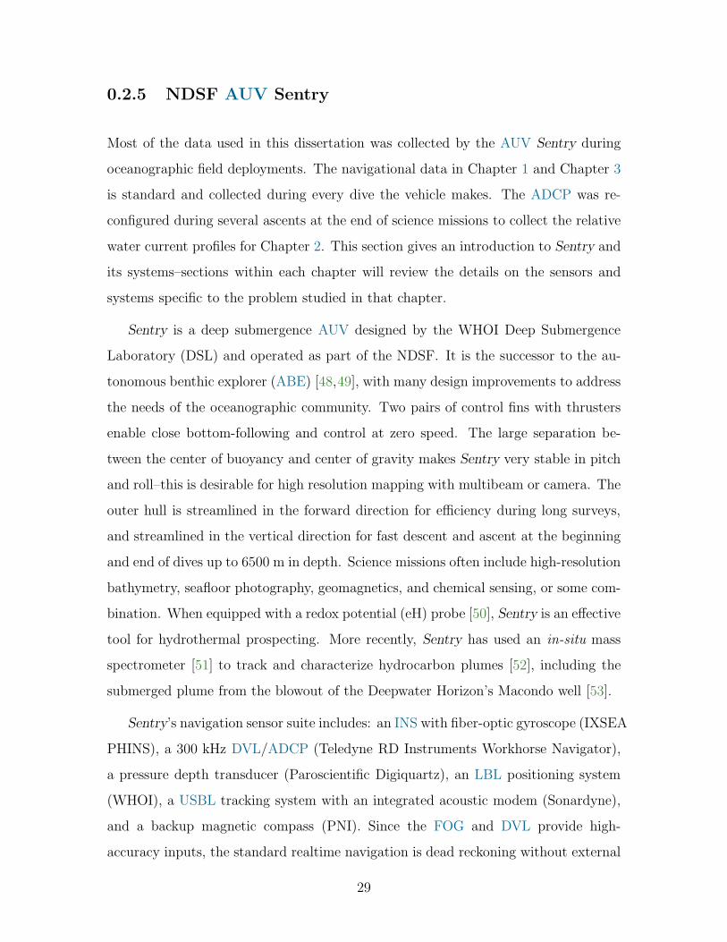
0.2.5 NDSF AUV Sentry
Most of the data used in this dissertation was collected by the AUV Sentry during
oceanographic field deployments. The navigational data in Chapter 1 and Chapter 3
is standard and collected during every dive the vehicle makes. The ADCP was re-
configured during several ascents at the end of science missions to collect the relative
water current profiles for Chapter 2. This section gives an introduction to Sentry and
its systems–sections within each chapter will review the details on the sensors and
systems specific to the problem studied in that chapter.
Sentry is a deep submergence AUV designed by the WHOI Deep Submergence
Laboratory (DSL) and operated as part of the NDSF. It is the successor to the au-
tonomous benthic explorer (ABE) [48,49], with many design improvements to address
the needs of the oceanographic community. Two pairs of control fins with thrusters
enable close bottom-following and control at zero speed. The large separation be-
tween the center of buoyancy and center of gravity makes Sentry very stable in pitch
and roll–this is desirable for high resolution mapping with multibeam or camera. The
outer hull is streamlined in the forward direction for efficiency during long surveys,
and streamlined in the vertical direction for fast descent and ascent at the beginning
and end of dives up to 6500 m in depth. Science missions often include high-resolution
bathymetry, seafloor photography, geomagnetics, and chemical sensing, or some com-
bination. When equipped with a redox potential (eH) probe [50], Sentry is an effective
tool for hydrothermal prospecting. More recently, Sentry has used an in-situ mass
spectrometer [51] to track and characterize hydrocarbon plumes [52], including the
submerged plume from the blowout of the Deepwater Horizon’s Macondo well [53].
Sentry’s navigation sensor suite includes: an INS with fiber-optic gyroscope (IXSEA
PHINS), a 300 kHz DVL/ADCP (Teledyne RD Instruments Workhorse Navigator),
a pressure depth transducer (Paroscientific Digiquartz), an LBL positioning system
(WHOI), a USBL tracking system with an integrated acoustic modem (Sonardyne),
and a backup magnetic compass (PNI). Since the FOG and DVL provide high-
accuracy inputs, the standard realtime navigation is dead reckoning without external
29

Figure 0-2: NDSF AUV Sentry being raised for launch. Two pairs of control fins withthrusters enable close bottom-following. The large separation between the center ofbuoyancy and center of gravity makes Sentry very stable in pitch and roll–this isdesirable for high resolution mapping with multibeam or camera.photo credit: Dana Yoerger, WHOI ABE/Sentry group
aiding. Navigation data is postprocessed after a dive to fuse external position inputs
before mapping timeseries data to geographic locations.
This high-quality navigation suite makes Sentry an ideal platform for evaluat-
ing alternate navigation methods and state estimators before implementing them on
vehicles with lower quality sensors.
The standard science sensor suite includes: a conductivity/temperature probe,
precision magnetometers, a 400 kHz multibeam sonar, and a 12-bit color camera.
Sentry serves the oceanographic community, with limited extra payload for systems
provided by scientists on each cruise. The vehicle has also carried redox potential
(eH) probes, dissolved oxygen sensors, an in-situ mass spectrometer, a sub-bottom
profiler, a sidescan sonar, and a stereo camera system.
0.3 Thesis Statement
This research explores three related hypotheses with the goal of improving the real-
time performance and increasing the level of automation in underwater navigation:
30

1. Rotors in Geometric Algebra can be used to formulate an elegant, efficient,
and stable realtime alignment estimator suitable for in-situ use on underwater
vehicles.
2. Relative water current profile data collected by a vehicle-mounted acoustic
Doppler current profiler can provide estimates of the global vehicle velocity
and position during descent and ascent phases of a mission.
3. Mathematically rigorous treatment of measurement delays in multi-sensor fusion
Kalman filters can be achieved through state augmentation and conditional
time-varying models without altering the underlying framework.
0.3.1 Objectives
This research has several objectives related to each hypothesis above.
Rotor identification
• formulate an adaptive identifier using rotors in Geometric Algebra (GA) for
sensor alignment
• prove asymptotic stability
• demonstrate rotation identification in simulation
• demonstrate DVL/FOG alignment identification
– using archival data from a laboratory ROV
– using data from an AUV deployed in the field
Independent navigation during descent and ascent
• formulate online bin average, least squares, and recursive least squares ap-
proaches
• collect data from AUV ascents
31

• demonstrate dead reckoned ascent using data from an AUV deployed in the
field
Fusing delayed measurements
• formalize an efficient model-driven approach that works within the Kalman
filter (KF) framework
• characterize performance of delayed measurement fusion using a simulation of
a canonical system
• demonstrate model-driven fusion of delayed acoustic positioning measurements
using data from an AUV deployed in the field performing
– USBL-aided DR
– asynchronous LBL-aided DR
0.4 Dissertation Structure
This chapter has provided a high-level introduction to underwater navigation and
an explicit statement of the thesis. The following chapters present each individual
contribution in detail:
Chapter 1 Navigation sensor alignment
This is a basic problem in any multi-sensor system–any uncertainties here pro-
pogate through the navigation system to the final result. Here I propose a stable
online method for in-situ alignment identification, and demonstrate it on data
from underwater vehicles in the laboratory and in the field. (Some of this work
is previously reported in [15].)
Chapter 2 Dead reckoning through the water column
The ability to link GPS at the surface to precision DR near the seafloor might
enable new kinds of missions for AUVs. This chapter introduces a method to
DR through the water column using water current profile data collected by
32

an onboard sensor, and provides an autonomous navigation link between the
surface and the seafloor without any dependence on a ship or external acoustic
tracking beacons. (Some of this work is previously reported in [28, 29].)
Chapter 3 Model-driven delayed measurement fusion
In many state estimation applications, delayed measurements present an in-
teresting challenge. Underwater navigation is a particularly compelling case
because of the relatively long delays inherent in all available position mea-
surements. Here I propose an entirely model-driven approach to delayed mea-
surement fusion based on state augmentation with a mathematically rigorous
treatment of the delay. (Some of this work is previously reported in [54].)
The last chapter of this dissertation briefly recapitulates the conclusions of each chap-
ter, and highlights some promising areas for future work.
33

34

Chapter 1
Navigation Sensor Alignment
Using Rotors
Hypothesis
Rotors in Geometric Algebra can be used to formulate an elegant, efficient, and stable
realtime alignment estimator suitable for in-situ use on underwater vehicles.
1.1 Introduction
Rotations are ubiquitous in robotics and engineering. Two examples are: industrial
robot arms move by rotating many different single degree-of-freedom joints, and the
misalignment between different sensors is the rotation between their internal reference
frames. We use Geometric Algebra (GA) to formulate a novel adaptive identifier for
unknown rotations, and apply it to an important problem in underwater navigation.
We develop this identifier using rotors, which provide an elegant and efficient treat-
ment of rotations (in multiple dimensions). More importantly, the GA formulation
expose the geometric nature of the problem, and encourage an intuitive solution.
The remainder of this introduction motivates and explicitly defines the general
problem of identifying an unknown three-dimensional rotation, then reviews exist-
ing approaches to rotation identification and other related work. To keep this paper
35

self-contained, section 1.2 provides a brief primer on the basics of GA, which may
be unfamiliar to many readers. This can be considered a section on the mathemat-
ical preliminaries for our approach–we only use GA basics in the formulation and
stability analysis of the identifier. Section 1.3 details the rotor identifier, including
the formulation, geometric intuition, a proof of asymptotic stability, and simulation
results. In section 1.4, we apply the new identifier to estimate the fine misalignment
between two important sensors in underwater navigation. We translate in-situ mea-
surement data into a form usable by the identifier using integration by parts. We
then demonstrate and characterize the performance of the identifier using data from
a remotely operated vehicle (ROV) in controlled laboratory conditions (Section 1.5),
and using field data from an autonomous underwater vehicle (AUV) operating in the
deep ocean (Section 1.6).
1.1.1 Motivation
This study is motivated by a common practical problem–identifying the unknown
alignment of two sensors using only the measurements from those sensors. This prob-
lem is of particular importance in robotic vehicle navigation, where data from many
separate sensors must be fused in a common frame of reference. In dead reckoning,
for example, a small alignment error leads to a large systematic position error in
time. Accurate identification of sensor alignment is therefore of utmost importance,
especially in applications like underwater navigation, where position updates may be
severely limited.
1.1.2 Problem: to identify a rotation from a pair of vectors
Consider two misaligned sensors that provide vector measurements. If the measure-
ment from the first sensor is u and the measurement of the second sensor is y, then
the relationship between the measurements is written:
y = R (u) , (1.1)
36

u
y
ϕ
(a)
e1
e2
e3
b
b
b
b
b
b
b
b
b
b
b
b
b
b b bb b
bbbbbbbbbbbbbbbbbbbbbb
bbbb
bbbbbb
bbbbbbbbbbbbbbbb
bb
bb
bbbbbb b
b b bb b b b b b
bbbbbbbbbbbbbbbbbbbbbbb
bb
bbbbbbbbbbb
b
(b)
Figure 1-1: The rotation between two vectors in two dimensions (a) is describedby a single parameter, the angle ϕ. The rotation is inherently constrained to thetwo-dimenstional plane. Identifying this rotation becomes more difficult in threedimensions–the plane of rotation is no longer constrained by the space (b). Theinput vector (red) could rotate along an infinite number of paths (purple) to reachthe output vector (blue).
where R (·) is a linear operator that describes the unknown rotation between the co-
ordinate frames of the sensors. The goal in aligning the measurements is to identify
the unknown R (·). This problem is simple in two dimensions–the rotation is fully
described by a single parameter (Figure 1-1a). But it is important to note the prob-
lem is underconstrained in higher dimensions–two vectors in 3-space do not uniquely
identify a rotation (Figure 1-1b).
Given enough measurements, this problem can be solved in Linear Algebra (LA)
using a conventional ordinary least squares (LS) approach to estimate the matrix that
best transforms the inputs u into the outputs y:
y = Mu (1.2)
but the result may not technically describe a rotation. Ordinary LS makes no guar-
antee that M will be a rotation matrix.
If the input/output relationship is restricted to rigid body rotations, the solution
must be part of the special orthogonal group.
y = Ru : R ∈ SO(3). (1.3)
In three dimensions, this is a subgroup of 3× 3 matrices subject to two constraints:
orthogonality columns of the matrix are orthogonal (i.e., independent)
37

normality scale and chirality1 are preserved
These constraints define the group of rotation matrices:
SO(3) ≡
R : R ∈ R3×3, RTR = I3×3, det (R) = 1
. (1.4)
The goal of the alignment problem in LA is to identify the matrix that best transforms
u into y, subject to the constraints of the special orthogonal group.
We propose a novel alternative approach using GA and encoding the rigid body
transformation in a rotor. The rotor acts on any element of GA by a double-sided
application of the geometric product:
y = RuR, u = RyR, R ∈ Spin(3). (1.5)
The algebraic structure of rotors inherently constrains all estimates to the group of
rigid-body rotations. The approach presented here also provides a clear interpretation
of the identifier using the first-order kinematics of the rotor estimate.
1.1.3 Related Work
This work is motivated by the practical problem of in-situ estimation of navigation
sensor alignment for dead reckoning (DR) for underwater vehicles. The problem
of Doppler velocity log (DVL)/fiber-optic gyroscope (FOG) alignment was first ad-
dressed by Kinsey & Whitcomb in [13,55]. They use measurements from an external
positioning system to observe the output of the DR plant. Using integration by parts,
they are able to write the plant in the identifier form (1.3), and then apply standard
and novel techniques to estimate the alignment.
This problem is a specific example of the more general problem of estimating rigid
body rotations from a collection of uncertain data. Approaches to this problem can
be loosely divided into batch methods and online methods. Much of the previous
1i.e., right-handed or left-handed. This mathematical property is also sometimes called orienta-tion, but we will reserve that term to describe rotational position since that is more in line with itscommon use in geometry and navigation.
38

literature has studied the problem using LA, but there are also some examples of
batch methods in GA. This section summarizes the related work in the literature.
Linear algebra, batch methods
Standard approaches to identify the matrix transforming input data to output data
include ordinary least squares and recursive least squares methods [56]. These meth-
ods are well-studied and their behavior is well characterized, but the solution is not
guaranteed to describe a rigid body rotation. That is, these methods may not actually
give a rotation matrix.
To enforce the orthogonality constraint on the LS solution, Arun et. al. introduce
an application of singular value decomposition (SVD) in [57].
Umeyama adapted the LS-SVD approach in [58] to also enforce the normality
constraint. The LS solution is now fully constrained to SO(3). This constrained least
squares (CLS) method is the present standard batch method for rotation identifica-
tion.
In [13,55], Kinsey & Whitcomb apply the LS-SO(3) batch method to estimate the
alignment between DVL and FOG in underwater navigation. The DR trajectories cal-
culated using the estimated alignment agreed with long baseline (LBL) observations
much better than those calculated using a rough visual alignment.
Linear algebra, online methods
The rotation identification problem is closely related to the attitude control problem.
Bullo & Murray study control on SO(3) and SE(3) using Lie groups2 in [60]. They
recognize the geodesic length as a natural error metric on SO(3). Assuming full state
feedback, they use Lyapunov theory to prove the stability of a family of proportional
and proportional-derivative control laws.
In [14,61] Kinsey & Whitcomb report an adaptive identifier on SO(3), and prove
its asymptotic stability using Lyapunov theory. They compare its performance to the
2Lie groups are actually closely related to rotors, and any Lie algebra can be expressed as abivector algebra [59].
39

LS methods in [13, 55] with favorable results.
More recently, Troni & Whitcomb have applied the LS methods and adaptive
identifier to identify the alignment between DVL and inertial navigation system
(INS) [62, 63]. This method no longer requires position measurements, so it has
no dependencies external to the vehicle, making it a strapdown solution. Instead, it
makes the mild assumption that the accelerometers and gyrocompass in the INS are
internally aligned and calibrated. This extra assumption is almost trivial since it is
done in manufacturing and does not need to be done in situ.
Geometric algebra, batch methods
Batch methods for rotor identification in GA have also been developed recently. Do-
ran studied the estimation of an unknown rotor from noisy data in the context of
camera localization in [64]. Buchholz and Sommer investigate the related problem of
averaging in Clifford groups [65].
1.1.4 Contributions
The online GA method detailed in this chapter is an asymptotically stable adap-
tive identifier and was originally proposed in [15]. This method works recursively
on input/output vector pairs and it uses a more compact and efficient encoding of
rotations than the LA methods. Furthermore, since rotors are inherently constrained
to represent rigid-body motions, no extra steps are required to constrain the solu-
tion. The rotor identifier is similar to the SO(3) adaptive identifer developed in [14],
but the GA formulation provides more meaningful and intuitive error measures (Sec-
tion 1.3.2) than LA approaches. This encourages a geometric understanding of the
problem and leads to a straightforward kinematic identification algorithm.
Table 2.1 compares this research to the related literature. The main contribution
of this work is the formulation of an online adaptive identifier using rotors. One of
the main advantages of using GA is the clarity it brings to the mathematical formu-
lation of the identifier and the proof of asymptotic stability3. The GA formulation
3A proof of exponential stability would require a complete observation of the rotation for each
40

Tab
le1.1:
Com
parison
ofrotoridentifier
torelatedwork.Filledcirclesdenotefeaturesor
characteristicsposessedbythework,
empty
circlesdenotefeaturesthat
aremissingor
not
dem
onstrated,an
dadashmeansthat
category
isnot
applicable.
method
batch
online
constraints
orthogonality
chirality
stability
asymptotic
exponential
uses
partialobservations
geodesicerror
representation
application
ordinaryLS(e.g.,[56])
•
--
•
matrix
general
Arun,et.al.[57]
•
•
--
•
matrix
machinevision
Umeyam
a[58]
•
••
--
•
matrix
machinevision
Doran
[64]
•
••
--
rotor
machinevision
Buchholz&
Som
mer
[ 65]
•
•
--
•
matrix&
rotor
general
Kinsey&
Whitcomb[ 13,55]
•
••
--
•
matrix
FOG/D
VLDR
Troni&
Whitcomb[62,63]
•
••
--
••
matrix
INS/D
VLDR
Bullo,
et.al.[60,66]
•
••
••
•
Lie
grou
psatellitecontrol
Kinsey&
Whitcomb[14,61]
•
••
•
•
matrix
FOG/D
VLDR
Stanway
&Kinsey[15]
&thischap
ter
•
••
•
••
rotor
FOG/D
VLDR
41

makes it easier to see how a simple proportional feedback regulator on the observable
output error can provide asymptotically stable identification. This clarity encourages
a more geometric understanding of the problem, and may simplify enhancements and
extensions of the identifier in the future.
1.2 Geometric Algebra Primer
This section provides an introduction to the GA tools used in this dissertation. It
is included because many readers may not be familiar with GA. It can be viewed
as a section on the mathematical preliminaries necessary to formulate the rotation
identifier and prove its stability. We only need the very basics of GA to do this.
For a more complete introduction to GA, the reader should refer to the introduc-
tory texts by Hestenes [67], Doran & Lasenby [68], or Dorst, Fontijne, & Mann [69].
Gull, et al., also provide an excellent short introduction in [70], and Bayro-Corrochano
discusses several engineering applications in [71–74]. Here, we will only cover the very
basics necessary for multiplying vectors and for representing rotations.
1.2.1 Multiplying Vectors
Every vector has two intrinsic properties: magnitude and direction. The products
defined in GA describe relationships between these properties. We will define the inner
product, the outer product, and the geometric product. These products then expand
the language of GA to include elements of lower and higher grade (i.e., dimension),
and even elements of mixed grade.
update of the estimate. Bullo assumes this in [60], but we cannot assume this in the FOG/DVLalignment problem that we apply the rotor identifier to in this research, because the observation ofthe rotation comes from pairs of input/output vectors (see section 1.1.2).
42

a
b
(a · b) a(a)
a
b
a
b
a ∧ b b ∧ a
(b)
Figure 1-2: The geometric product is the sum of symmetric and antisymmetric parts:the inner product of two vectors (a) is symmetric and produces a scalar, the outerproduct of two vectors (b) is antisymmetric and produces a bivector.
Inner Product
We will start with a familiar concept–the inner product of two vectors is commutative,
and defines a scalar α (grade 0):
a · b = b · a = α = |a||b| cosϕ, (1.6)
where ϕ is the angle between a and b. The inner product vanishes if the vectors are
perpendicular, but if they are parallel, it becomes the product of the magnitudes.
This provides one way to define the magnitude of a vector:
|a| = √a · a. (1.7)
This inner product should be familiar to the reader since it is essentially the same as
in Linear Algebra.
Outer Product
The outer product of two vectors is anticommutative and defines a new entity called
a bivector4 B (grade 2):
a ∧ b = −b ∧ a = B = |a||b| sinϕB. (1.8)
4Bivectors in GA are analogous in many ways to skew-symmetric matrices in LA, and both arerelated to Lie algebras.
43

This bivector can be thought of as a directed plane segment in much the same way
as a vector is a directed line segment. Unit bivectors, like B, define a direction and
have a magnitude of one. New bivectors can be generated by addition or subtraction.
The outer product is associative and can be used to build up even higher-grade
elements, like trivectors T (grade 3):
(a ∧ b) ∧ c = a ∧ (b ∧ c) = T = βI. (1.9)
Trivectors are the highest grade element inG3, the three-dimensional Euclidean model
of GA. Every trivector can be written as a scalar (e.g. β) times the unit trivector, so
the unit trivector is called the pseudoscalar and denoted by I. Since no set of four
or more vectors in G3 is independent5, the outer product of four or more vectors is
always zero.
Geometric Product
The inner and outer products complement each other: one lowers the grade while
the other raises it, one is commutative while the other is anticommutative. They are
combined in the geometric product:
ab = a · b+ a ∧ b = b · a− b ∧ a = α +B =M, (1.10)
which produces a multivector M that contains both scalar and bivector parts.
The geometric product is actually the most basic product in GA. The inner and
outer products can be derived axiomatically as the symmetric and antisymmetric
components of the geometric product [67, 68].
a · b = 1
2(ab+ ba) (1.11a)
a ∧ b = 1
2(ab− ba) (1.11b)
5This is true for any three-dimensional linear space.
44

The geometric product itself is generally neither commutative nor anticommuta-
tive. But reversing the order of factors is still an important operation, known as
reversion:
reverse(ab) = ba = (ab)∼ = M. (1.12)
Sometimes it is useful to separate a multivector into parts of just one grade (i.e., se-
lect only the grade 2 part, the bivector). This operation is called grade selection, and
denoted by angle brackets with the grade as a subscript:
〈M〉0 = α, 〈M〉2 = B. (1.13)
In general, a multivector can be a sum of elements of all grades: A = α+a+B+βI.
It may seem odd at first to add together elements of different grades, but it is really no
different than adding together the real and imaginary parts of a complex number [70].
In fact, the constructs of GA are closely related to complex numbers and quaternions,
which brings us to the topic of rotations.
1.2.2 Rotating vectors
Rotations in GA are encoded by special elements called rotors. These describe a
rotation in a plane, rather than around an axis–this extends more readily to spaces
that are not 3D Euclidean (i.e., 2D plane, 4D projective, or 5D conformal). Any
multivector can be transformed using rotors: simply left-multiply by the rotor, and
right-multiply by its reverse:
M ′ = RMR. (1.14)
This double-sided application of the geometric product is sometimes called the versor
or sandwich product. This transformation works equally well in two dimensions, three
dimensions, or even more6.
6In fact, rotors in Conformal Geometric Algebra describe general rigid body motions, encodingboth rotation and translation in a single entity [68, 75].
45

a
nb
m
c
(a)
B
uθ
y
(b)
Rα
RβR
(c)
Figure 1-3: Three main methods of composing rotors: (a) from two vectors using theconcept of repeated reflections, (b) from a bivector using the exponential map, or (c)from two or more other rotors as a chain.
Definition
The set of rotors, or proper unitary spinors, is given by the normalized elements of the
even subalgebra G+. In a three-dimensional Euclidean space, they form the group:
Spin(3) ≡
R : R ∈ G+3 , RR = RR = 1
, (1.15)
which is isomorphic to the quaternions H, but with emphasis on geometric interpreta-
tion and easily extended to higher dimensional spaces. Spin(3) provides a double-cover
over SO(3).
Three-dimensional rotors have four coefficients: one scalar and three bivectors.
The orthogonality constraint is implicit in the structure. The unit norm constraint is
simple to enforce, but often unneccesary because of good numerical stability proper-
ties [76–78]. In contrast, rotation matrices have nine coefficients, and orthonormality
is more difficult to ensure.
Composition
There are three main methods to compose a rotor (Figure 1-3): (i) using the concept
of repeated reflections, (ii) as the geometric exponential of a bivector, or (iii) chaining
together a sequence of multiple rotors. We use all of them in the formulation and
stability proof of the identifier.
46

Repeated reflections
The Cartan-Dieudonne theorem states that any Euclidean transformation can be
expressed by a combination of reflections [79]. This suggests the first method of rotor
composition: repeated reflections.
The sandwich product using a unit vector on each side:
z = nun. (1.16)
produces a reflection. Any combination with an even number of reflections will pro-
duce a proper7 rotation. So rotors are the geometric product of an even number of
unit vectors:
y = RuR = mnunm. (1.17)
An even number of repeated reflections (as opposed to a single reflection) are required
to ensure right-handed coordinates remain right-handed.
This method of composing a rotor is particularly useful when you need to calculate
the ‘shortest’ rotor between two vectors. Choose the first unit vector in the direction
of the first vector. Then add the two vectors and normalize the sum to get the
second unit vector. This one points in the direction that bisects the angle between
the original vectors, as shown in Figure 1-3a.
Bivector exponential
In the second rotor composition method, a bivector encodes the plane and angle
(i.e., the direction and magnitude) of the rotation. The rotor that generates this
rotation is the exponential8 of the bivector:
R = exp
(
−1
2θB
)
= e−1
2B, (1.18)
7Conversely, an odd number of reflections produces an improper rotation, or rotoreflection.8The concept of an exponential function is easily generalized to operate on multivectors, see [67]
or [68].
47

where the factor of 1/2 is because we multiply the rotor twice (once on each side) and
the negative sign is a convention so that positive angles produce a counterclockwise
(i.e., right-handed) rotation.
It is also useful to define a multivector logarithm so that the bivector B can be
determined from the rotor R. This actually has some subtle points, but is well-defined
for rotors. We adopt the definition given in [67] and denote the rotor logarithm:
B = −2 lnR. (1.19)
Rotor chains
The rotor group is closed under multiplication with the geometric product. This leads
to a third way to compose rotors–as a chain of two or more other rotors:
Ra
(
RbuRb
)
Ra = (RaRb) u(
RbRa
)
= RabuRab. (1.20)
The geometric product of two rotors will always produce another rotor. This property
is very useful for discrete-time kinematics.
GA is a much richer topic–the interested reader should refer to texts referenced
at the beginning of this section. Having covered the very basics, we now have all the
tools we need to build our identifier and study its properties.
1.3 Asymptotically Stable Rotor Identifier
Here we propose an adaptive identifier based on first-order rotor kinematics and a
geometric interpretation of identification error. We will begin by defining the rotation
plant in terms of input and output vectors. Then we discuss several possible error
metrics, with emphasis on the geometric meaning of each of them. We use first-
order rotor kinematics and a proportional gain error-state feedback regulator (ESFR)
to formulate a rotor identifier, then prove its asymptotic stability using Lyapunov
theory. This section concludes with a brief discussion of gain selection.
48

1.3.1 Plant Definition
Given known input u and output y signals of the same grade9, the plant:
y = RuR, (1.21)
describes the rotation from input to output. The unknown rotor R ∈ Spin(3) is a
stationary element of the even subalgebra, and encodes a rigid body rotation. The
goal of the method proposed here is to identify this unknown rotor, R.
We will define the time-varying estimate of the rotor as S(t) ∈ Spin(3). The
expected plant output is then:
v = SuS. (1.22)
We will call (1.22) the identification plant.
The goal of the identifier is to drive the estimated rotor S toward the actual rotor
R. Since each timestep provides an incomplete observation of the actual rotor, we
achieve this using feedback on the output error. The action of the identifier drives
the expected output v toward the observed output y.
1.3.2 Error Metrics
This problem has two types of error: the parameter error describes the difference
between the estimated and actual values; the output error describes the difference
between the estimated and observed outputs. These errors can be parameterized in
several ways–GA encourages a geometric interpretation of each parameterization and
of the relationships between them. Defining an error rotor is natural because the
goal is to identify a rotor in the first place. A bivector error can be directly applied
to drive the first order kinematics as a rotational velocity. Finally, a scalar error is
most convenient for summarizing performance and in Lyapunov analysis. Here we
9 We focus on vector signals (u, y ∈ 〈G3〉1) for the remainder of this paper. However, the methodspresented here should apply equally well to bivectors or to higher-grade multivectors, so long as thegrade of the output is the same as the grade of the input–otherwise (1.21) and (1.22) would notdescribe rotations.
49

define these three error metrics for both types of error. We discuss their geometric
interpretation and the relationships between them.
Parameter Error
Define the parameter error rotor:
Q = RS : Q ∈ Spin(3). (1.23)
This definition gives the ‘difference’ between the estimated rotor and the actual rotor.
Applying the parameter error rotor directly to the estimated output will rotate it into
the actual output:
QvQ = (RS)(SuS)(SR)
= RuR = y
The error rotor is the geometric operator that resolves the difference between the
identification plant and the actual plant.
The parameter error bivector is derived from the natural logarithm of the param-
eter error rotor:
X = −2 ln(Q) : Q = e−1
2X . (1.24)
This metric encodes both the magnitude and direction of the error, which can be
interpreted as the angle and the rotation plane.
The magnitude of the parameter error is a scalar:
χ = ||X||1/2 =√
XX. (1.25)
This is the natural distance measure on S3, and concisely summarizes the error state.
It is distilled down to the angle between the estimate and the truth, and is analogous
to the distance measure defined in [60]. As a scalar, χ is convenient for visualization
and for stability analysis, but the lack of directional information makes it less useful
50

for feedback.
Output Error
Since a pair of input/output vectors does not uniquely define a rotation, the param-
eter error is only partially observed at each timestep. We define output errors to
characterize the observable part of the misalignment.
The output error rotor is defined:
P = mn =y + v
|y + v|v
|v| : P ∈ Spin(3), (1.26)
so that it rotates the estimated output v directly into the measured output y along
the shortest path on the sphere10. Note that (1.26) uses the concept of repeated
reflections (1.17) to compose P .
The output error bivector is defined analogously to its parameter error counter-
part11:
Y = −2 ln(P ). (1.27)
This bivector form of the output error encodes information on both magnitude and
direction–we will show in section 1.3.3 how it can be used as a rotational velocity to
drive the identification plant kinematics.
Similar to (1.25), the output error angle is:
ψ = ||Y ||1/2 =√
Y Y . (1.28)
Again, this scalar provides a useful summary of the parameter error, but the lack of
directional information makes it unsuitable for feedback.
Each of these error measures is valid, and each has a different use and interpre-
10In [69], Dorst gives an alternate form for the ‘shortest’ rotor between two vectors:R = (1 + ba) /
√
2 (1 + a · b) This is equivalent to (1.26) for a = v and b = y.11There are, of course, alternate ways to define the output error bivector. We have chosen to
define Y this way for consistency with X in (1.24) and so that its magnitude leads directly tothe arc length of the error. Moreover, (1.26) normalizes the vectors y + v and v to emphasize thedifference in direction and not magnitude. This is one difference from the approach in [14].
51

tation. Note that the error rotors tend toward unity as S → R, while the bivectors
and angles tend toward zero.
Partial observation and error bivectors
The output error bivector is only part of the parameter error bivector–there may
also be an unobserved component, Z, orthogonal to the observed output error. This
is because a rotation defined only by two vectors is not unique, as noted earlier
in section 1.1.2. The parameter error bivector is the sum of these two parts:
X = Y + Z, where: Z ⊥ Y. (1.29)
Note that the orthogonality condition is a weak constraint on the unobserved component–
Z can have any magnitude12 or direction as long as it is not parallel to Y .
Despite this limitation, a straighforward proportional gain feedback regulator on
the observed output error is an asymptotically stable adaptive identifier.
1.3.3 Proportional Gain Identifier
Now that we have a clear understanding of the underlying geometry of this problem,
we can formulate a simple identifier based on proportional feedback into the first
order kinematics of the system.
First-Order Kinematics
We are interested in the time derivative of the rotor estimate S(t) ∈ Spin(3). Recall
the exponential parameterization of the rotor:
S(t) = e−1
2B(t). (1.30)
12Strictly speaking, the bivector errors may have any magnitude. In practice, this is limited tothe interval [0, 2π).
52
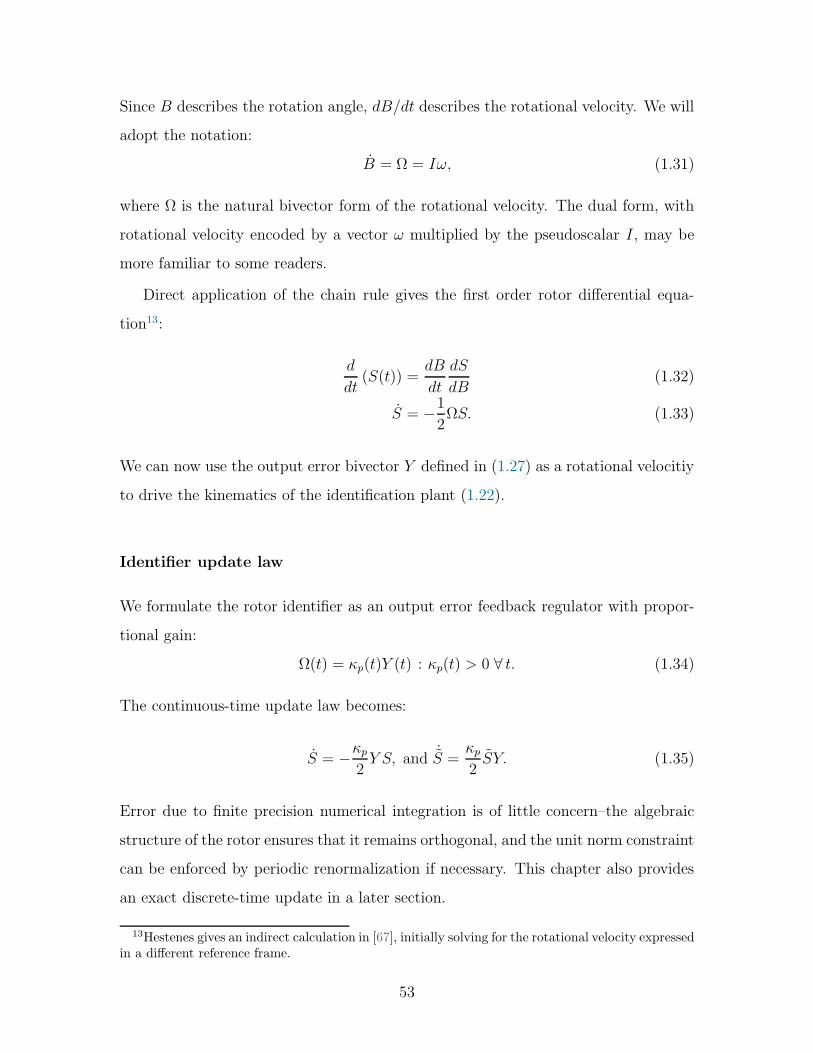
Since B describes the rotation angle, dB/dt describes the rotational velocity. We will
adopt the notation:
B = Ω = Iω, (1.31)
where Ω is the natural bivector form of the rotational velocity. The dual form, with
rotational velocity encoded by a vector ω multiplied by the pseudoscalar I, may be
more familiar to some readers.
Direct application of the chain rule gives the first order rotor differential equa-
tion13:
d
dt(S(t)) =
dB
dt
dS
dB(1.32)
S = −1
2ΩS. (1.33)
We can now use the output error bivector Y defined in (1.27) as a rotational velocitiy
to drive the kinematics of the identification plant (1.22).
Identifier update law
We formulate the rotor identifier as an output error feedback regulator with propor-
tional gain:
Ω(t) = κp(t)Y (t) : κp(t) > 0 ∀ t. (1.34)
The continuous-time update law becomes:
S = −κp2Y S, and ˙S =
κp2SY. (1.35)
Error due to finite precision numerical integration is of little concern–the algebraic
structure of the rotor ensures that it remains orthogonal, and the unit norm constraint
can be enforced by periodic renormalization if necessary. This chapter also provides
an exact discrete-time update in a later section.
13Hestenes gives an indirect calculation in [67], initially solving for the rotational velocity expressedin a different reference frame.
53

Parameter Error Evolution
The evolution of the estimate is characterized by the time derivative of the parameter
error rotor:
Q = RS +R ˙S = R ˙S. (1.36)
Substituting the update law (1.35) gives the continuous-time system:
Q = R(κp2SY
)
=κp2QY. (1.37)
This looks very similar to the first-order rotor differential equation (1.33). In fact, (1.37)
simply states that the rotational velocity of the parameter error is proportional and
opposite to the rotational velocity of the estimate.
Q = −1
2XQ, (1.38)
−X = 2QQ = κpQY Q = Ω′, (1.39)
where Ω′ is the rotational velocity expressed in the reference frame of R.
Discrete-time implementation
Most applications will provide measurements of the input u and the output y in
discrete time, so it makes sense to develop a discrete-time version of the proportional
update law (1.35).
Define the discrete update of the rotor estimate:
δS = SkSk−1 : Sk = (δS)(Sk−1). (1.40)
Assuming the gain and rotational velocity of the rotor estimate are constant over the
timestep, we use Euler’s method to integrate (1.35) directly:
δS =
δt∫
0
(
−κp2Y S
)
dτ = e−1
2(κpδt)Y . (1.41)
54

0 5 10 15 20 25 30 35 40
timestep
−1.0
−0.5
0.0
0.5
1.0
rotorcomponents
scalar
e1 ∧ e2
e2 ∧ e3
e3 ∧ e1
Figure 1-4: The components of the estimated rotor S computed by the proportionalgain rotor identifier converge to the components of the unknown rotor R (marked bydash-dot lines).
This discrete-time form of the rotor identifier was implemented in C using a base
library generated by Gaigen2.5 [80], the latest version of the GA implementation
generator [81, 82].
Figure 1-4 shows the four components of the estimated rotor S converging toward
the true rotor R in a simulation using the discrete-time rotor identifier. In other
simulations, several levels of random Gaussian noise were added to the output y.
Figure 1-5 shows how the scalar parameter error χ decreases in time until it reaches
the level of the noise.
1.3.4 Asymptotic Stability
We employ Lyapunov theory [83, 84] to prove the stability of (1.35). This involves
identifying an energy-like scalar function of the error, then showing that the time
derivative of this function does not increase.
55

0 100 200 300 400 500
timestep
10−17
10−15
10−13
10−11
10−9
10−7
10−5
10−3
10−1
χ[rad]
σν = 10−2
σν = 10−4
σν = 10−6
σν = 0
Figure 1-5: Evolution of the scalar parameter error when the input/output vectorpairs are corrupted by additive white noise. The estimated rotor converges to theactual rotor until χ approaches the noise floor. The estimate then oscillates aroundthe truth with magnitude controlled by the gain and the noise level.
Lyapunov Candidate Function
We choose a Lyapunov candidate using the natural distance measure on S3, which is
the parameter error angle χ:
V =1
2χ2. (1.42a)
This function is analagous to the Lyapunov functions employed in [14, 60]. By ex-
panding the parameter error angle χ the Lyapunov candidate function can also be
written directly in terms of the parameter error rotor:
V = 2 lnQ ln Q, (1.42b)
or the parameter error bivector:
V =1
2‖X‖2 = 1
2XX. (1.42c)
56
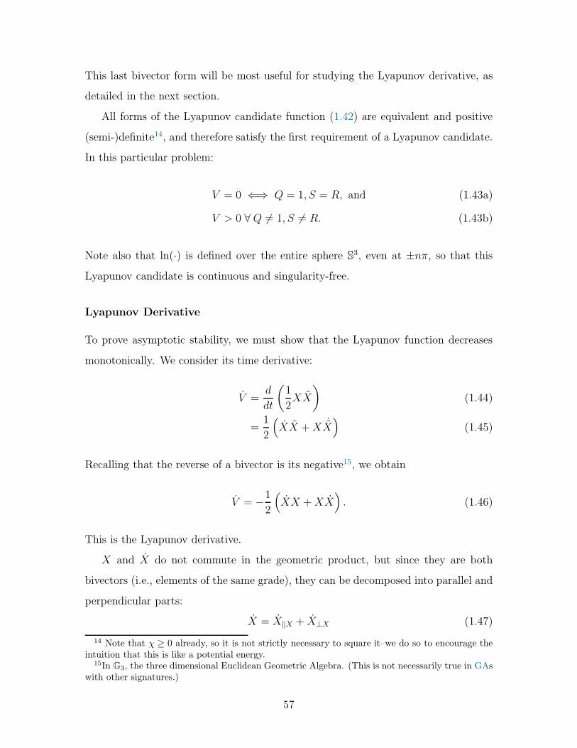
This last bivector form will be most useful for studying the Lyapunov derivative, as
detailed in the next section.
All forms of the Lyapunov candidate function (1.42) are equivalent and positive
(semi-)definite14, and therefore satisfy the first requirement of a Lyapunov candidate.
In this particular problem:
V = 0 ⇐⇒ Q = 1, S = R, and (1.43a)
V > 0 ∀Q 6= 1, S 6= R. (1.43b)
Note also that ln(·) is defined over the entire sphere S3, even at ±nπ, so that this
Lyapunov candidate is continuous and singularity-free.
Lyapunov Derivative
To prove asymptotic stability, we must show that the Lyapunov function decreases
monotonically. We consider its time derivative:
V =d
dt
(
1
2XX
)
(1.44)
=1
2
(
XX +X ˙X)
(1.45)
Recalling that the reverse of a bivector is its negative15, we obtain
V = −1
2
(
XX +XX)
. (1.46)
This is the Lyapunov derivative.
X and X do not commute in the geometric product, but since they are both
bivectors (i.e., elements of the same grade), they can be decomposed into parallel and
perpendicular parts:
X = X‖X + X⊥X (1.47)
14 Note that χ ≥ 0 already, so it is not strictly necessary to square it–we do so to encourage theintuition that this is like a potential energy.
15In G3, the three dimensional Euclidean Geometric Algebra. (This is not necessarily true in GAswith other signatures.)
57
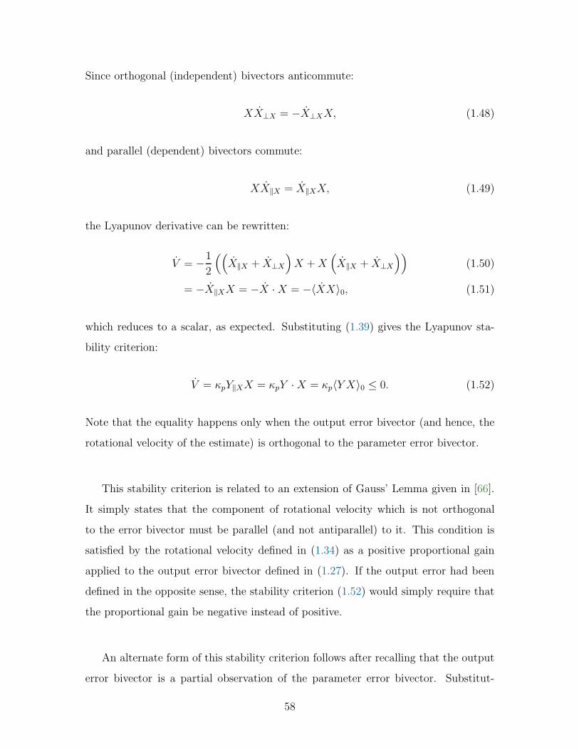
Since orthogonal (independent) bivectors anticommute:
XX⊥X = −X⊥XX, (1.48)
and parallel (dependent) bivectors commute:
XX‖X = X‖XX, (1.49)
the Lyapunov derivative can be rewritten:
V = −1
2
((
X‖X + X⊥X
)
X +X(
X‖X + X⊥X
))
(1.50)
= −X‖XX = −X ·X = −〈XX〉0, (1.51)
which reduces to a scalar, as expected. Substituting (1.39) gives the Lyapunov sta-
bility criterion:
V = κpY‖XX = κpY ·X = κp〈Y X〉0 ≤ 0. (1.52)
Note that the equality happens only when the output error bivector (and hence, the
rotational velocity of the estimate) is orthogonal to the parameter error bivector.
This stability criterion is related to an extension of Gauss’ Lemma given in [66].
It simply states that the component of rotational velocity which is not orthogonal
to the error bivector must be parallel (and not antiparallel) to it. This condition is
satisfied by the rotational velocity defined in (1.34) as a positive proportional gain
applied to the output error bivector defined in (1.27). If the output error had been
defined in the opposite sense, the stability criterion (1.52) would simply require that
the proportional gain be negative instead of positive.
An alternate form of this stability criterion follows after recalling that the output
error bivector is a partial observation of the parameter error bivector. Substitut-
58
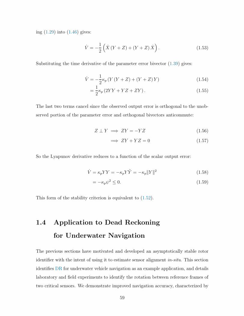
ing (1.29) into (1.46) gives:
V = −1
2
(
X (Y + Z) + (Y + Z) X)
. (1.53)
Substituting the time derivative of the parameter error bivector (1.39) gives:
V = −1
2κp (Y (Y + Z) + (Y + Z)Y ) (1.54)
=1
2κp (2Y Y + Y Z + ZY ) . (1.55)
The last two terms cancel since the observed output error is orthogonal to the unob-
served portion of the parameter error and orthogonal bivectors anticommute:
Z ⊥ Y =⇒ ZY = −Y Z (1.56)
=⇒ ZY + Y Z = 0 (1.57)
So the Lyapunov derivative reduces to a function of the scalar output error:
V = κpY Y = −κpY Y = −κp‖Y ‖2 (1.58)
= −κpψ2 ≤ 0. (1.59)
This form of the stability criterion is equivalent to (1.52).
1.4 Application to Dead Reckoning
for Underwater Navigation
The previous sections have motivated and developed an asymptotically stable rotor
identifier with the intent of using it to estimate sensor alignment in-situ. This section
identifies DR for underwater vehicle navigation as an example application, and details
laboratory and field experiments to identify the rotation between reference frames of
two critical sensors. We demonstrate improved navigation accuracy, characterized by
59

100
10−9
10−18
10−27
10−36
V
0 50 100 150 200 250
timestep
100
10−9
10−18
10−27
10−36
−V
Figure 1-6: Time evolution of the Lyapunov function V and its derivative V . TheLyapunov function decreases monotonically as the rotor estimate S approaches theactual rotor R, until the scalar error reaches the noise level of the measurements.
0.00 0.01 0.02 0.03 0.04 0.05 0.06 0.07 0.08
V
−0.025
−0.020
−0.015
−0.010
−0.005
0.000
V
Figure 1-7: Phase-space trajectory of the Lyapunov function V for twenty tests withrandom data. As the rotor estimate S evolves in time, the system approaches equi-librium at the origin.
lower residuals in observations on the DR vehicle position.
60

0 200 400 600 800 1000
timestep
10−20
10−18
10−16
10−14
10−12
10−10
10−8
10−6
10−4
10−2
100
χ/χ0
machine precision limit
mean
median
extrema
σ
Figure 1-8: Evolution of the scalar parameter error, normalized by its initial value.Results are ensemble-averaged over twenty randomly generated datasets and com-pared for four proportional gains: κp ∈ 0.001, 0.01, 0.1, 0.25.
1.4.1 Dead Reckoning and the Identification Plant
Position-velocity form using Linear Algebra
The first-order kinematic equation for a vehicle moving in the navigation frame (de-
noted by a superscript n) is:
pn(t) = pn(0) +
t∫
0
un(τ)dτ, (1.60)
where p is the position vector and u is the velocity vector.
Rotating the velocities into the vehicle frame (denoted by a superscript v) gives
the first-order DR equation:
pn(t) = pn(0) +
t∫
0
Rvn(τ)u
v(τ)dτ (1.61)
61

The DVL reports velocities in the instrument frame, so (1.61) is rewritten:
pn(t) = pn(0) +
t∫
0
Rvn(τ)R
ivu
i(τ)dτ (1.62)
where Rvi ∈ SO(3) is the matrix describing the time invariant rotation from instru-
ment coordinates to vehicle coordinates. This is the rotation we are trying to identify.
The position of the vehicle in the navigation frame, pn, is measured by LBL or
ultra-short baseline (USBL). The rotation from the vehicle frame to the navigation
frame is computed from the attitude measured by the North-seeking gyrocompass16,
and can be expressed by the rotation matrix Rvn(τ). The DVL measures the vehi-
cle velocity in the instrument frame, ui(τ). We are left with the unknown sensor
alignment, expressed by the rotation matrix Rvi .
The task now is to transform (1.62) with the available inputs into a form compat-
ible with the identifier plant. Here we review the approach taken in [13, 14]17.
Differentiating (1.62) in time gives:
pn(t) = Rvn(t)R
ivu
i(t) (1.63)
Rotating both sides of the equation into the vehicle frame:
Rnv(t)p
n(t) = Rivu
i(t) (1.64)
brings us to the form of the identification plant.
However, the signal pn(t) is not generally available in situ in the field. Numerical
differentiation of LBL position measurements in the field is impractical due to delays
and relatively high noise level. However, integrating the left hand side of (1.64) by
16This can be applied with any attitude/orientation reference (e.g. magnetic compass, attitudeand heading reference system (AHRS), gyrocompass, FOG, ring-laser gyroscope (RLG), inertialmeasurement unit (IMU), or INS). The application in this research is to identify the misalignmentbetween a FOG-based North-seeking gyrocompass and a DVL, so we will use the acronym FOG forbrevity.
17A formulation of the DR or INS equations in GA may be an interesting topic for future research.
62

parts gives:
∫
Rnv(τ)p
n(τ)dτ = Rnv(t)p
n(t)−∫
Rnv(τ)p
n(τ)dτ + const. (1.65)
This removes the unavailable signal pn(τ), but introduces the new parameter Rnv(τ).
The new signal may be measured directly by the FOG, or it may be numerically
differentiated (since the update rate is higher, delay is negligible, and noise is lower
for the FOG than with LBL).
Since Rvi is stationary the integral of the right hand side of (1.64) is:
∫
Rivu
i(τ)dτ = Riv
∫
ui(τ)dτ (1.66)
And now we have an equation in the form of the identifier plant using measurements
that are available in situ:
Rnv(t)p
n(t)−∫
Rnv(τ)p
n(τ)dτ + const. = Riv
∫
ui(τ)dτ (1.67)
This maps to the identifier (1.3):
y = Ru (1.68)
with the input:
u =
∫
ui(τ)dτ (1.69)
the output:
y = Rnv(t)p
n(t)−∫
Rnv(τ)p
n(τ)dτ + const. (1.70)
63

In all laboratory and field experiments, the means of the input u and output y are
shifted to zero so that only the rotation remains. This is the form Kinsey &Whitcomb
used in [13, 14] to identify the alignment between a FOG and DVL.
1.4.2 Renavigation and performance metrics
The goal of the DVL/FOG alignment problem is to improve DR navigation. To
experimentally validate the rotor identifier, we compare DR trajectories calculated
with the rotor alignment estimate to LBL observations. We will characterize the
improvement in DR performance gained by using the rotor alignment estimate versus
a visual alignment estimate. We will also compare to the alignment methods in [13,14].
All of this analysis is done in post-processing by renavigating the same raw sensor
data using each alignment estimate.
Position residual
First, we calculate the difference between the DR estimate and the LBL measurement
of vehicle position–this is the position residual18:
p = pnDR − pn
LBL (1.71a)
x
y
z
=
xnDR − xnLBL
ynDR − xnLBL
znDR − znLBL
(1.71b)
As an example, (Figure 1-9) shows the components of the position residual in lab-
oratory experiment 070. We will use several aspects of this position residual as
performance metrics.
Residual component distributions
The components of the position residual (1.71b) are sorted into bins, and the distri-
bution is plotted for the residual along each direction. The horizontal axis will show
18The tilde decoration here on p denotes the residual, not the reversion operation in GA.
64

−0.10
−0.05
0.00
0.05
0.10
North
visual
−0.10
−0.05
0.00
0.05
0.10
East
0 3000 6000 9000
timestep
−1.0
−0.5
0.0
0.5
1.0
Down
ID-Spin(3)
0 3000 6000 9000
timestep
Figure 1-9: Components of the position residual from laboratory experiment 070. Inthe left column, residuals from DR with the visual alignment estimate are plotted ingray. In the right column, residuals from DR with the ID-Spin(3) alignment estimateare plotted in green. Note that the vertical component of the residual from the visualalignment is much larger than the others, and that the ID-Spin(3) alignment reducesit considerably.
65

0
2
4
6
8
10
12
14
16
18
0
2
4
6
8
10
12
14
16
−0.15 −0.10 −0.05 0.00 0.05 0.10 0.15
residual [m]
0
5
10
15
20
25
30
North
East
Down
norm
alizeddensity
Figure 1-10: Distributions of the position residual components from laboratory ex-periment 070.
the residual, and the vertical axis will show the frequency–this is normalized so that
it integrates to one. (Figure 1-10)
66

Residual component standard deviations
To summarize the residual component distributions, we compute standard deviation
of the residual in each direction. These are collected into the residual component
standard deviation vector19:
σ =
σx
σy
σz
=
std (xnDR − xnLBL)
std (ynDR − ynLBL)
std (znDR − znLBL)
(1.72)
The Euclidean norm of this vector:
‖σ‖2 =√σσT (1.73)
is termed the standard deviation vector norm20. This provides a convenient scalar per-
formance metric that is suitable for computing ensemble statistics for cross-validation
of each alignment estimate across the other datasets.
Residual magnitude distribution
Alternatively, we may consider the Euclidean norm of the position residual at each
point in time:
‖p‖2 =√
ppT . (1.74)
Since the magnitude of p is always positive, this produces a one-sided distribution
(Figure 1-11). Again, the frequency axis is normalized so that the distribution inte-
grates to one.
We will also study the integral of this distribution–the cumulative residual mag-
nitude distribution. This provides another perspective on the residual–it shows the
fraction of the residuals that fall below a certain magnitude. For example, Figure 1-12
19This is called the error vector in [13, 14, 85].20This is called the error vector norm in [13, 14, 85].
67

0.00 0.02 0.04 0.06 0.08 0.10 0.12 0.14 0.16
residual norm, ‖p‖2 [m]
0
5
10
15
20
25
30
norm
alizeddensity
Figure 1-11: Distribution of the position residual magnitude from laboratory experi-ment 070.
0.00 0.02 0.04 0.06 0.08 0.10 0.12 0.14 0.16
residual norm, ‖p‖2 [m]
0.0
0.2
0.4
0.6
0.8
1.0
norm
alizedcumulativedensity
Figure 1-12: Cumulative distribution of the position residual magnitude from labo-ratory experiment 070.
shows that half of the position residual vectors are less than 5.3 centimeters long, and
90% of them are less than 9.4 centimeters long.
Mean and median residual magnitude
Since the residual magnitude distribution is one-sided, we will use its mean and
median to summarize it. For self-validation tests (renavigating the same dataset that
68

was used to estimate the rotation) we will show standard deviations as well.
Different alignment methods
We will compare DR trajectories using four alignment methods:
visual This is the initial alignment estimate with beam 3 of the DVL pointing down
and toward the forward starboard quarter. The alignment mark on the DVL
housing points straight ahead–the DVL coordinate frame is misaligned from the
FOG coordinate frame by 45 (π/2 rad) in heading and 0 in roll and pitch.
LS-SO(3) The batch method from [58] to estimate the rotation matrix using LS
constrained to SO(3) as applied to DVL/FOG alignment in [13, 55].
ID-SO(3) The adaptive identifier on SO(3) from [14, 61]. This has been slighly
modified by normalizing the input u and output y fed to the identifier. This
change preserves directional information in the measurements, but changes the
behavior of the identifier with respect to gains. It was necessary for the identifier
to work on field datasets from Sentry.
ID-Spin(3) The adaptive identifier on Spin(3), the group of rotors in G3. This is
the method detailed in [15] and earlier in this chapter.
1.5 Laboratory Experiments
This section evaluates the performance of the rotor identifier on the FOG/DVL align-
ment problem using data from controlled experiments with a laboratory ROV. This
data is from the same series of six experiments used in [13,14,85], and results from the
rotor identifier are compared to those from the CLS and SO(3) alignment methods
reported there.
Section 1.5.1 briefly reviews the experimental setup and conditions21 given in [13,
14,85]. The rotor identification results and renavigated trajectories from each exper-
21By necessity, much of this is paraphrased from [13, 14, 85]; it is reviewed here for completeness.
69

Figure 1-13: The Johns Hopkins University ROV is a laboratory system outfittedwith sensors similar to those typically found on oceanographic research vehicles. Itis a testbed vehicle used for for dynamics, control, and navigation studies for deepsubmergence vehicles. (photo credit: JHU DSCL)
iment are given in section 1.5.2, and alignment cross-validation between the different
experiments is discussed in section 1.5.3.
1.5.1 JHU Hydrodynamics Test Facility and JHUROV
Data in these experiments was collected in the Hydrodynamics Test Facility at the
Johns Hopkins University (JHU). JHUROV (Figure 1-13) is a testbed vehicle for
dynamics, control, and navigation studies for deep submergence vehicles. It is in-
strumented with sensors similar to those found on vehicles in the field, except that
some of the laboratory systems have shorter range and higher precision. The sensors
relevant to this study are listed in Table 1.2.
The pressure depth transducer (Paroscientific Digiquartz) is precise to 10 parts
70

Table 1.2: Navigation sensors on JHUROV used in laboratory experiments. (adaptedfrom [13, 14, 85])
quantity sensor sample rate precision range
(x, y) position300 kHz LBL
5 Hz 5e−3 m 100 m(Marquest) SHARPS
depthpressure transducer
7 Hz 1e−4 m 10 m(Paroscientific Digiquartz)
orientationfiber-optic gyroscope (FOG)
10 Hz0.01 360
(IXSEA PHINS) 1.7e−4rad 2πrad
velocity1200 kHz DVL
10 Hz 0.3% ∼ 30 m(TRDI WHN)
per million over a depth of 10 meters at 7 Hz. A two-beacon 300 kHz LBL system
(Marquest) provides (x, y) position measurements at rates up to 18 Hz. Combined
with the depth constraint, the position is accurate to within 7 mm at one standard
deviation [85]. Velocity over ground is measured by a 1200 kHz DVL (Teledyne
RD Instruments Workhorse Navigator) with precision22 better than 0.3% at 5-10 Hz.
Vehicle heading is measured within 0.05 and roll & pitch within 0.01 at a rate of 10
Hz by a FOG (Ixsea PHINS). In these experiments, the FOG did not record angular
rates, so they are obtained by numerical differentiation [85].
More details on the Hydrodynamics Test Facility and JHUROV can be found
in [85, 86].
1.5.2 Alignment identification and renavigated trajectory
The rotor identifier was used to estimate DVL/FOG alignment on JHUROV on each
of six laboratory experiments. The closed-loop trajectories were each 40 minutes long
to collect enough data for the LS estimator while avoiding potential problems from
unmodeled DR integration drift [85]. Data from expt070 was used to introduce the
renavigation error metrics in section 1.4.2.
Figure 1-14 shows the normalized distribution of the residual magnitude. The DR
track using the visial alignment estimate disagrees with the LBL observations by more
than one meter in some places. The alignment estimated by the rotor identifier brings
22standard deviation of error in velocity component measured along a single acoustic beam
71

0.0 0.2 0.4 0.6 0.8 1.0 1.2 1.4
residual norm, ‖p‖2 [m]
0
5
10
15
20
25
norm
alizeddensity
visual
LS-SO(3)
ID-SO(3)
ID-Spin(3)
0.00 0.02 0.04 0.06 0.08 0.10 0.12 0.14
residual norm, ‖p‖2 [m]
0
5
10
15
20
25
norm
alizeddensity
visual
LS-SO(3)
ID-SO(3)
ID-Spin(3)
Figure 1-14: Residual magnitude distribution or JHUROV laboratory dataset 070,renavigated using different DVL/FOG alignment estimates. The lower figure is azoom into the left side of the upper figure, to see the small differences between thealignment methods. Vertical lines indicate the mean of the residual magnitude. Notethat the rotor identifier presented here performs comparably to the LS-SO(3) batchmethod in [13] and the ID-SO(3) method with normalized inputs, adapted from [14].All three methods perform significantly better than the visual alignment estimate.
72

0.0 0.2 0.4 0.6 0.8 1.0 1.2 1.4
residual norm, ‖p‖2 [m]
0.0
0.2
0.4
0.6
0.8
1.0
visual
LS-SO(3)
ID-SO(3)
ID-Spin(3)
norm
alizedcumulativedensity
0.00 0.02 0.04 0.06 0.08 0.10 0.12 0.14
residual norm, ‖p‖2 [m]
0.0
0.2
0.4
0.6
0.8
1.0
visual
LS-SO(3)
ID-SO(3)
ID-Spin(3)
norm
alizedcumulativedensity
Figure 1-15: Cumulative residual magnitude distribution for JHUROV laboratorydataset 070, renavigated using different DVL/FOG alignment estimates. The lowerfigure is a zoom into the left side of the upper figure, to see the small differences be-tween the alignment methods. Note that the rotor identifier presented here performscomparably to the LS-SO(3) batch method in [13] and the ID-SO(3) method withnormalized inputs, adapted from [14]. All three methods perform significantly betterthan the visual alignment estimate.
all residuals within fourteen centimeters, and the rotor identifier performs comparably
to LS-SO(3) and ID-SO(3) methods.
Figure 1-15 shows the normalized cumulative distribution of the residual magni-
tude. This plot makes it easy to determine what fraction of the residuals fall below a
particular level. For example, 50% of the residuals in expt070 fall below 5.3 cm when
73

DR uses the alignment estimate from the rotor identifier, but that same fraction of
residuals extends as high as 53 cm magnitude using the visual alignment estimate.
The other laboratory datasets show similar results. When using the alignment
from the rotor identifier:
• The residual component distributions are narrower, closer to zero from both
sides.
• The one-sided residual magnitude distribution is weighted to the left, in the
range of centimeters rather than tens of centimeters.
• The residual magnitude cumulative distribution becomes much steeper and
moves toward the upper left corner, showing again that the residuals are much
smaller.
The effect of using the ID-SO(3) or ID-SO(3) alignment estimate is similar–the rotor
identifier performs comparably to these previous results.
Table 1.3 shows the summarized statistics of the renavigation residuals for all six
laboratory experiments. In this data, the residuals in depth are the largest starting
with the visual alignment estimate, and using the alignment estimated by the rotor
identifier reduces them considerably. Using the alignment estimated by the rotor
identifier reduces the standard deviation vector norm to 10-15% of its original value
with the visual alignment estimate. The mean and median of the magnitude of the
residuals are similarly reduced. Figure 1-16 shows these quantities graphically. Again,
the rotor identifier performs comparably to the previously reported rotation matrix
methods, and all of these perform better than the original visual alignment method.
Of course, the performance improvement will always depend on how close the visual
alignment estimate is in the first place.
1.5.3 Cross-validation
It is reasonable to ask how the alignment estimated using one dataset performs on
another. If the sensors are not moved between experiments, the estimated alignment
74

Tab
le1.3:
Positionresidual
statistics
afterrenavigationof
laboratorydatasetscollectedbyJHUROV.
dataset
alignment
σNorth
σEast
σdep
th‖σ
‖‖σ‖
‖σvisual‖
mean‖p
‖median‖p
‖method
expt063
visual
0.048941
0.051171
0.562006
0.566449
1.000000
0.493259
0.477453
LS-SO(3)
0.048044
0.045893
0.026068
0.071372
0.125999
0.065268
0.062575
ID-SO(3)
0.049499
0.045983
0.031374
0.074491
0.131505
0.068100
0.064871
ID-Spin(3)
0.049080
0.045934
0.021666
0.070627
0.124683
0.063832
0.061798
expt064
visual
0.054306
0.055148
0.559550
0.564878
1.000000
0.491591
0.477783
LS-SO(3)
0.050364
0.052372
0.026778
0.077437
0.137086
0.071144
0.069237
ID-SO(3)
0.051481
0.052184
0.024861
0.077405
0.137030
0.070971
0.068505
ID-Spin(3)
0.051152
0.052090
0.023962
0.076838
0.136026
0.070451
0.068020
expt066
visual
0.055127
0.063670
0.634868
0.640429
1.000000
0.561986
0.539055
LS-SO(3)
0.051213
0.081422
0.016910
0.097664
0.152498
0.089230
0.087373
ID-SO(3)
0.049993
0.080407
0.018780
0.096526
0.150721
0.088191
0.085575
ID-Spin(3)
0.049093
0.079424
0.018137
0.095117
0.148521
0.086825
0.083930
expt067
visual
0.045764
0.054911
0.652066
0.655972
1.000000
0.575595
0.593576
LS-SO(3)
0.056585
0.067803
0.018521
0.090234
0.137558
0.080677
0.077294
ID-SO(3)
0.037244
0.053945
0.021890
0.069111
0.105356
0.060573
0.056939
ID-Spin(3)
0.038036
0.057167
0.019969
0.071509
0.109012
0.062514
0.057791
expt069
visual
0.050956
0.061569
0.593581
0.598937
1.000000
0.523565
0.527018
LS-SO(3)
0.047439
0.053742
0.019076
0.074179
0.123850
0.067636
0.065466
ID-SO(3)
0.045226
0.052778
0.018236
0.071857
0.119974
0.065144
0.063387
ID-Spin(3)
0.046041
0.053130
0.021236
0.073441
0.122618
0.066976
0.065171
expt070
visual
0.060111
0.053238
0.624291
0.629433
1.000000
0.552794
0.531055
LS-SO(3)
0.040129
0.040330
0.027860
0.063349
0.100645
0.058784
0.054766
ID-SO(3)
0.042558
0.040951
0.030262
0.066363
0.105432
0.061415
0.057304
ID-Spin(3)
0.041485
0.040701
0.020898
0.061760
0.098120
0.056765
0.052385
75

063 064 066 067 069 0700.00
0.05
0.10
0.15
0.20
0.25
‖σ‖/‖σ
visual‖
LS-SO(3) ID-SO(3) ID-Spin(3)
063 064 066 067 069 0700.00
0.05
0.10
0.15
0.20
0.25
residualnorm
,‖p‖ LS-SO(3) ID-SO(3) ID-Spin(3)
Figure 1-16: Self-validation of alignment estimates for each laboratory dataset.Barplot shows the normalized standard deviation vector norm as defined in (1.73)and represent the improvement in navigation over the original (visual) alignmentestimate. Boxplot shows the residual norm for each experiment.
76

should perform comparably on other trajectories. Figure 1-17 shows the normalized
standard deviation vector magnitude using the alignment estimated from each labo-
ratory dataset to renavigate the trajectory of each other dataset for each of the three
different alignment methods. The plots show fairly uniform levels with some lower
magnitudes along the diagonal. This should be expected, and indicates that the best
renavigation performance is on the same dataset used for the estimate. Figure 1-18
collects this data into ensembles and displays the statistics for each alignment estimate
renavigating every other dataset. The normalized standard deviation vector magni-
tude is comparable across alignment estimates–this indicates good cross-validation
of the estimates. Again, the rotor identifier performs comparably to the previously
reported rotation matrix methods.
1.5.4 A note on transient response
Unlike batch methods for estimating a rotation, the adaptive identifiers are dynamic
systems. It can be important to consider the transient response of such systems,
especially when they will be subject to unknown excitation (e.g. measurement noise).
Figure 1-19 compares the time history of the ID-SO(3) and ID-Spin(3) identifiers on
expt070, using a scalar (geodesic) residual with the estimate from the batch LS-SO(3)
method as a reference. It is important to note that this is experimental data without
a ground truth, so the LS-SO(3) may not be more correct than either of the others.
Both adaptive identifiers initially converge toward the same rotation estimate as
the LS-SO(3) method, within about 10−3 radians. The interesting event to note is
that the identifier estimates fluctuate between input/output vector pairs 4000 and
8000. The magnitude of the input u and output y is initially large, and both pass
through zero near vector pair 6000, before increasing in magnitude again. This is
because the means of u and y were set to zero when mapping the DR measurements
into the form of the identifier (Section 1.4.1). As u and y pass through zero, any noise
in the measurements becomes proportionally larger, and the identifiers will react to
that noise.
This problem can be handled pragmatically in this application by averaging the
77

LS-SO(3)
063 064 066 067 069 070
renavigated on
063
064
066
067
069
070
alignmentfrom
0.00
0.05
0.10
0.15
0.20
‖σ‖
‖σ
visual‖
ID-SO(3)
063 064 066 067 069 070
renavigated on
063
064
066
067
069
070
alignmentfrom
0.00
0.05
0.10
0.15
0.20
‖σ‖
‖σ
visual‖
ID-Spin(3)
063 064 066 067 069 070
renavigated on
063
064
066
067
069
070
alignmentfrom
0.00
0.05
0.10
0.15
0.20
‖σ‖
‖σ
visual‖
Figure 1-17: Cross-validation of alignment estimates on each other laboratory dataset.Colors indicate the magnitude of the normalized standard deviation vector.
78

063 064 066 067 069 0700.00
0.05
0.10
0.15
0.20
0.25
‖σ‖
‖σ
visual‖
LS-SO(3) ID-SO(3) ID-Spin(3)
063 064 066 067 069 0700.00
0.05
0.10
0.15
0.20
0.25
‖σ‖
‖σ
visual‖
LS-SO(3) ID-SO(3) ID-Spin(3)
Figure 1-18: Cross-validation statistics of alignment estimates over all laboratorydatasets. The alignment estimate from one dataset was used to renavigate the datafrom all other datasets. Bars show the mean normalized magnitude of the standarddeviation vector, and whiskers indicate the standard deviation of this magnitudeacross the other datasets. Boxplots show the median, first quartile, and total rangeof the normalized magnitude of the standard deviation vector.
79

0 2000 4000 6000 8000 10000 12000 14000
input/output vector pair
10−4
10−3
10−2
10−1
100
residualvs.
LS-SO(3)[rad]
ID-SO(3)
ID-Spin(3)
Figure 1-19: Scalar residual with respect to alignment estimated by LS-SO(3) method.
estimated rotor23 over several timesteps. This particular behavior may not be im-
portant in other applications of rotation identification–it depends on how the inputs
and outputs vary. Nevertheless, it raises an interesting question: what modifications
might enable the rotor identifier to reject noise better? One approach might involve
adding some damping to the system–using both proportional and derivative gains in
the output error feedback regulator. This seems like an obvious next step, but keep
in mind that is due mostly to the clarity offered by the GA formulation–this behavior
of the transient response was effectively illustrated with a scalar residual, and the
simple interpretation of the identifier as a regulator was enabled by working in rotors
and bivectors.
1.6 Field Experiments
This section evaluates the performance of the rotor identifier on the FOG/DVL align-
ment problem using data from field deployments of the oceanographic AUV Sentry.
Results from the rotor identifier are compared to those from the CLS and SO(3)
alignment methods reported in [13, 14].
23 This is another area where the GA formulation is useful–it is much easier to average rotorsthan rotation matrices (see, e.g. [64, 65]).
80

Table 1.4: Navigation sensors on Sentry used in field experiments.quantity sensor sample rate precision range
(x, y) position12 kHz LBL
0.1 Hz ∼ 0.25 m > 10000 m(WHOI)
depthpressure transducer
7 Hz 0.02 m 6500 m(Paroscientific Digiquartz)
orientationfiber-optic gyroscope (FOG)
10 Hz0.01 360
(IXSEA PHINS) 1.7e−4rad 2πrad
velocity300 kHz DVL
2 Hz 0.3% ∼ 200 m(TRDI WHN)
Section 1.6.1 briefly reviews Sentry and its navigation sensors. The rotor identi-
fication results and renavigated trajectories from each experiment are given in sec-
tion 1.6.2, and alignment cross-validation between the different experiments is dis-
cussed in section 1.6.3.
1.6.1 Sentry field deployments on the Hakon Mosby mud
volcano
The rotor identifier was applied to navigational data from Sentry field deployments on
the Hakon Mosby mud volcano in the Barents Sea. These dives were part of a research
cruise led by Dr. Antje Boetius with the goal of characterizing the bathymetry, sub-
bottom composition, and chemistry surrounding the mud volcano. The Sentry team
deployed and surveyed a LBL net of three transponders for six24 dives on the same
site.
A brief overview of the AUV Sentry (Figure 1-20) is given in section 0.2.5. Specific
to the problem in this section, we will be using navigational data from the sensors
listed in Table 1.4, comparing DR vehicle trajectories to LBL observations.
81

Figure 1-20: The NDSF AUV Sentry is an unmanned oceanographic research vehiclethat dives as deep as 6500 meters to perform various scientific missions. Sentrynavigates primarily by DR with a FOG and DVL. The FOG is located in the mainpressure housing, roughly amidships and just below the name label. The DVL ison the keel just aft from the bow. The large separation between these sensors on avehicle that may deform under extreme pressure (even slightly), motivates our studyof stable, in-situ sensor alignment methods. (photo credit: D Yoerger, ABE/SentryGroup, WHOI)
1.6.2 Alignment identification and renavigated trajectory
Figure 1-21 shows the normalized distribution of each component of the residual, and
Figure 1-22 shows the normalized distribution of the residual magnitude for Sen-
try075. The magnitude distribution of the residuals is shifted slightly left (i.e.,
smaller) when using the alignment from the rotor identifier vs. the visual estimate.
This is also reflected in the mean of the distribution. Again, the rotor identifier
performs comparably to the previously reported rotation matrix methods.
Figure 1-23 shows the normalized cumulative distribution of the residual magni-
tude. This plot makes it easy to determine what fraction of the residuals fall below
a particular level. For example, 50% of the residuals in Sentry075 fall below 3.3 m
when DR uses the alignment estimate from the rotor identifier, but that same fraction
24The last dive of the cruise, Sentry078, was terminated early due to an actuator failure andimminent weather. Data from that dive is not used in this section.
82

0.00
0.05
0.10
0.15
0.20
0.25
0.000.020.040.060.080.100.120.140.160.18
−10 −5 0 5 10
residual [m]
0.0
0.2
0.4
0.6
0.8
1.0
visual
LS-SO(3)
ID-SO(3)
ID-Spin(3)
North
East
Down
norm
alizeddensity
Figure 1-21: Distributions of residual components for Sentry075, renavigated usingdifferent DVL/FOG alignment estimates. Note that the rotor identifier presentedhere performs comparably to the LS-SO(3) batch method in [13] and the ID-SO(3)method with normalized inputs, adapted from [14].
83

0 2 4 6 8 10
residual norm, ‖p‖2 [m]
0.00
0.05
0.10
0.15
0.20
0.25
0.30
0.35
0.40
norm
alizeddensity
visual
LS-SO(3)
ID-SO(3)
ID-Spin(3)
Figure 1-22: Residual magnitude distribution for Sentry075, renavigated using differ-ent DVL/FOG alignment estimates. Vertical lines indicate the mean of the residualmagnitude. Note that the rotor identifier presented here performs comparably to theLS-SO(3) batch method in [13] and the ID-SO(3) method with normalized inputs,adapted from [14].
0 2 4 6 8 10
residual norm, ‖p‖2 [m]
0.0
0.2
0.4
0.6
0.8
1.0
visual
LS-SO(3)
ID-SO(3)
ID-Spin(3)
norm
alizedcumulativedensity
Figure 1-23: Cumulative residual magnitude distribution for Sentry075, renavigatedusing different DVL/FOG alignment estimates. Note that the rotor identifier pre-sented here performs comparably to the LS-SO(3) batch method in [13] and theID-SO(3) method with normalized inputs, adapted from [14].
84
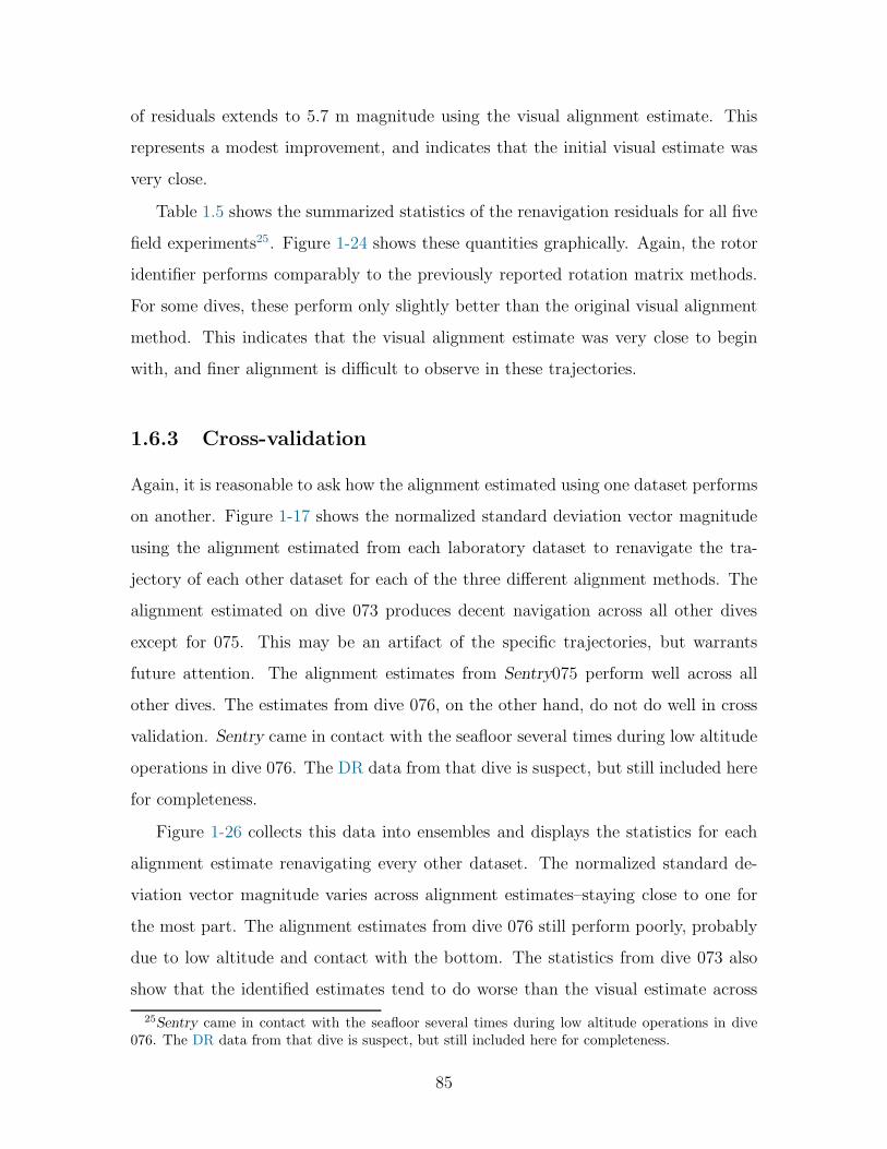
of residuals extends to 5.7 m magnitude using the visual alignment estimate. This
represents a modest improvement, and indicates that the initial visual estimate was
very close.
Table 1.5 shows the summarized statistics of the renavigation residuals for all five
field experiments25. Figure 1-24 shows these quantities graphically. Again, the rotor
identifier performs comparably to the previously reported rotation matrix methods.
For some dives, these perform only slightly better than the original visual alignment
method. This indicates that the visual alignment estimate was very close to begin
with, and finer alignment is difficult to observe in these trajectories.
1.6.3 Cross-validation
Again, it is reasonable to ask how the alignment estimated using one dataset performs
on another. Figure 1-17 shows the normalized standard deviation vector magnitude
using the alignment estimated from each laboratory dataset to renavigate the tra-
jectory of each other dataset for each of the three different alignment methods. The
alignment estimated on dive 073 produces decent navigation across all other dives
except for 075. This may be an artifact of the specific trajectories, but warrants
future attention. The alignment estimates from Sentry075 perform well across all
other dives. The estimates from dive 076, on the other hand, do not do well in cross
validation. Sentry came in contact with the seafloor several times during low altitude
operations in dive 076. The DR data from that dive is suspect, but still included here
for completeness.
Figure 1-26 collects this data into ensembles and displays the statistics for each
alignment estimate renavigating every other dataset. The normalized standard de-
viation vector magnitude varies across alignment estimates–staying close to one for
the most part. The alignment estimates from dive 076 still perform poorly, probably
due to low altitude and contact with the bottom. The statistics from dive 073 also
show that the identified estimates tend to do worse than the visual estimate across
25Sentry came in contact with the seafloor several times during low altitude operations in dive076. The DR data from that dive is suspect, but still included here for completeness.
85

Tab
le1.5:
Position
residual
statisticsafter
renavigation
offield
datasets
collectedbySentry
.
dataset
alignment
σNorth
σEast
σdep
th‖σ‖
‖σ‖
‖σvisual ‖
mean
‖p‖
median
‖p‖
meth
od
sentry
073
visu
al4.925604
7.0240440.199698
8.5812971.000000
7.6267686.779823
LS-SO(3)
3.1077036.747554
4.0000948.437302
0.9832207.834738
7.582955ID
-SO(3)
2.8212796.756833
2.5195657.743553
0.9023767.020782
6.495987ID
-Spin(3)
2.8860016.755998
3.3447968.072185
0.9406727.369756
6.960915
sentry
074
visu
al2.097726
1.4926690.570155
2.6369661.000000
2.4854432.453175
LS-SO(3)
2.0828781.223801
0.1227102.418911
0.9173082.274189
2.264834ID
-SO(3)
2.0917711.361575
0.4839442.542360
0.9641232.396811
2.369539ID
-Spin(3)
2.0898101.317990
0.3168062.490938
0.9446232.342860
2.332514
sentry
075
visu
al3.464273
1.6991595.669578
6.8580201.000000
6.1600245.700183
LS-SO(3)
3.5454741.823476
2.2463714.576203
0.6672774.201113
4.155020ID
-SO(3)
3.5813541.714496
0.4476833.995750
0.5826393.485687
3.222189ID
-Spin(3)
3.5962131.696875
0.4677184.003859
0.5838213.489983
3.242537
sentry
076
visu
al5.554410
1.8542645.938688
8.3401311.000000
7.2770206.342527
LS-SO(3)
5.7914690.743226
1.2864565.979002
0.7168954.311404
2.746244ID
-SO(3)
5.7618850.850114
1.6527506.054222
0.7259144.501826
2.912722ID
-Spin(3)
5.7646330.738832
1.9844266.141238
0.7363484.592775
2.975477
sentry
077
visu
al1.264703
2.8077971.114158
3.2748351.000000
2.9337202.768180
LS-SO(3)
1.2178052.753298
0.3082483.026337
0.9241192.636209
2.552532ID
-SO(3)
1.2009902.745069
0.2045033.003266
0.9170742.607675
2.519493ID
-Spin(3)
1.1698402.751775
0.4227303.019849
0.9221382.643394
2.551747
86

073 074 075 076 0770.0
0.2
0.4
0.6
0.8
1.0
1.2
1.4
1.6
‖σ‖/‖σ
visual‖
LS-SO(3) ID-SO(3) ID-Spin(3)
073 074 075 076 0770
2
4
6
8
10
12
14
16
residualnorm
,‖p‖ LS-SO(3) ID-SO(3) ID-Spin(3)
Figure 1-24: Self-validation of alignment estimates for each field dataset.
the other datasets. Sentry 073 covered more distance at higher altitude, with little
change in depth–a trajectory that may not have provided enough information for any
of the identifiers. Again, the rotor identifier performs comparably to the previously
reported rotation matrix methods.
1.7 Discussion and Conclusions
This chapter has presented a novel alternative approach to the sensor alignment
problem. Rotations are encoded using rotors in Geometric Algebra, so that algebraic
87

LS-SO(3)
073 074 075 076 077
renavigated on
073
074
075
076
077
alignmentfrom
0.0
0.2
0.4
0.6
0.8
1.0
1.2
1.4
1.6
1.8
‖σ‖
‖σ
visual‖
ID-SO(3)
073 074 075 076 077
renavigated on
073
074
075
076
077
alignmentfrom
0.0
0.2
0.4
0.6
0.8
1.0
1.2
1.4
1.6
1.8
‖σ‖
‖σ
visual‖
ID-Spin(3)
073 074 075 076 077
renavigated on
073
074
075
076
077
alignmentfrom
0.0
0.2
0.4
0.6
0.8
1.0
1.2
1.4
1.6
1.8
‖σ‖
‖σ
visual‖
Figure 1-25: Cross-validation of alignment estimates on each other field dataset.Colors indicate the magnitude of the normalized standard deviation vector.
88
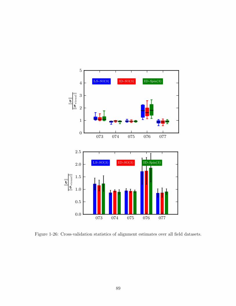
073 074 075 076 0770
1
2
3
4
5‖σ‖
‖σ
visual‖
LS-SO(3) ID-SO(3) ID-Spin(3)
073 074 075 076 0770.0
0.5
1.0
1.5
2.0
2.5
‖σ‖
‖σ
visual‖
LS-SO(3) ID-SO(3) ID-Spin(3)
Figure 1-26: Cross-validation statistics of alignment estimates over all field datasets.
89

structure implicitly constrains parameter estimates to describe rigid body rotations.
We proposed a stable adaptive identifier in section 1.3, and proved its stability using
Lyapunov theory on the continuous-time system. We then provided an equivalent
discrete-time implementation of the identifier. Numerical simulations illustrated the
behavior of the identifier under persistent excitation. These simulations showed that
the identifier provides an accurate estimate of the true rotor, up to the level of noise in
the input signals. Section 1.4.2 provided the necessary information to apply the rotor
identifier to the DVL/FOG alignment problem for DR in underwater navigation, and
defined several performance metrics. Section 1.5 applied the rotor identifier to identify
DVL/FOG alignment on an ROV operating in controlled laboratory conditions, and
section 1.6 demonstrated the rotor identifier using field data from the AUV Sentry.
In the end, the rotor identifier improved DR performance comparably to previously
reported rotation matrix methods. The Geometric Algebra formulation provides a
clear kinematic interpretation of the proposed rotor identifier, which provides accu-
rate, stable alignment estimates. It may offer a clearer path forward in improving
online alignment identifiers, including, for example, enhanced noise rejection using a
proportional-derivative feedback formulation. It may also prove useful in formulating
an identifier for full rigid body motions–including rotation and translation–which can
be encoded using rotors in higher dimensions.
90

Chapter 2
Dead Reckoning Through the
Water Column
Hypothesis
Relative water current profile data collected by a vehicle-mounted acoustic Doppler
current profiler can provide estimates of the global vehicle velocity and position during
descent and ascent phases of a mission.
2.1 Introduction
This chapter presents methods for dead reckoning through the water column, pro-
viding a navigation link between Global Positioning System (GPS) at the surface
and dead reckoning (DR) at the seafloor, without relying on external systems. The
methods use overlapping water profile measurements from an acoustic Doppler cur-
rent profiler (ADCP) to simultaneously estimate the vehicle velocity and the ocean
current profile.
Despite recent advances in technology and processing, underwater navigation re-
mains a challenging problem. Signals from the GPS are only available at the beginning
and the end of a mission, when the vehicle is on the surface. When it is near the
seafloor, a vehicle can estimate its position by dead reckoning with a compass and a
91

Doppler velocity log (DVL) in bottom-lock. In some cases, the vehicle can further
improve its position estimate using information from the terrain (e.g., bathymetry or
photography). Inertial navigation can provide good navigation in the short-term, but
quality sensors are expensive and the solution is subject to drift in the long term..
There is a significant portion of each mission–during the descent and the ascent–where
GPS and bottom-lock DVL measurements are unavailable, and the vehicle will drift
in the ocean current.
Underwater vehicles currently rely on acoustic positioning methods for localization
in the water column. Popular approaches include long baseline (LBL) transponder
nets, or ship-mounted ultra-short baseline (USBL) tracking systems with an acoustic
modem to downlink position fixes. However, these systems both require valuable ship
time. This external dependence also limits the autonomy of the underwater vehicle.
This chapter proposes a method to enhance the independent navigation capability of
underwater vehicles, and discusses the challenges encountered in making this method
work in the field.
The remainder of this section introduces the basic idea of DR using water profile
data from an ADCP, then briefly reviews related work in the literature. Section 2.2
outlines the concept of operations. Section 2.3 gives details on the setup and imple-
mentation for three different approaches to solve the problem. Section 2.4 illustrates
real-world performance and challenges using field data collected by the autonomous
underwater vehicle (AUV) Sentry fromWoods Hole Oceanographic Institution (WHOI).
Finally, Section 2.5 summarizes the results of the field experiences and discusses the
feasibility of an underwater navigation system operating entirely independent of ex-
ternal acoustic tracking.
92

2.1.1 To navigate from the surface to the seafloor and back
Many underwater vehicles use a DVL for DR when they are near the seafloor1. The
hardware and operating principles for a DVL and an ADCP are the same–comparing
the Doppler shift of an acoustic signal along four different beams gives the velocity
of an acoustic scatterer relative to the instrument. For a DVL in bottom-lock, the
scatterer is the seafloor; for an ADCP, the scatterers are particles suspended in the
water column. The same instrument can measure the relative velocity of the bottom
and the ocean current.
Overlapping water current profiles measured by a vehicle-mounted ADCP can
provide simultaneous estimates of the local ocean current and the vehicle velocity.
This velocity can then be used for dead reckoning. It could also be used as an aiding
input to an inertial navigation system (INS), but the method proposed here does not
rely on an INS–it only requires an ADCP, depth sensor, and attitude reference. The
goal is to develop a method that is applicable to many types of underwater vehicles
with different grades of sensors, but flexible enough to be fused with other navigation
methods where resources permit.
The approach presented here relies on three basic assumptions:
1. The vehicle starts or ends its transit with a global velocity estimate (e.g., from
GPS or DVL bottom lock).
2. The vehicle can measure overlapping partial ocean current profiles relative to
its own motion.
3. The ocean current may vary with depth, but the current at each depth is slowly
varying in time. (i.e., The current is constant over the timescale of the ascent,
on the order of minutes.)
If these conditions are satisfied, the vehicle can maintain an estimate of its global
velocity as well as the ocean current as it transits through the water column.
1i.e., within the frequency dependent bottom-track range of the DVL: ∼ 246 meters for a 300kHz DVL, ∼ 94 meters for a 600 kHz DVL, or ∼ 25 meters for a 1200 kHz DVL (assuming 50 VDCsupply) [17].
93

2.1.2 Related Work
The physical oceanography community has used ship-mounted ADCPs for many years
to measure current profiles in the open ocean. In deep water the limited range2 of the
ADCP prevents a ship-mounted instrument from obtaining a full current profile. Re-
searchers address this shortcoming by mounting an ADCP on an instrument package
that is lowered from the ship on a cable. The current profile from the Lowered Acous-
tic Doppler Current Profiler (LADCP) was initially computed by depth-averaging the
vertical shear across the individual ensembles [25, 26]. The present standard least
squares (LS) batch processing method, proposed in [27], is more flexible for incor-
porating additional constraints, like bottom-track velocities and average velocity of
the instrument package. This LADCP method is the standard approach to measure
current profiles in the deep ocean.
Recently, there has been interest in using the DVL already onboard most deep
submergence vehicles as an ADCP to simultaneously estimate vehicle velocity and
ocean current. The vehicle velocity can then be used for DR through the water
column. That is the goal of the research presented in this chapter. Preliminary
work toward this goal was presented in in [28], demonstrating an online bin-average
implementation in simulation and on field data collected by an AUV. An alternative
approach, presented in [30], couples ADCP current profiles with inertial measurement
unit (IMU) measurements in an information filter (IF) framework. This IF approach
was later demonstrated on shallow field deployments with a high-frequency (1200
kHz) ADCP in [31]. Field experiences navigating the ascent from several deep dives
with a low-frequency (300 kHz) ADCP are reported in [29], using the online bin
average approach, as well as LS and recursive least squares (RLS) formulations of the
problem.
2The nominal water profiling range of a 300 kHz ADCP is 135 meters, but actual usable rangedepends on supply voltage and bin size [17].
94

Table 2.1: Comparison of DR through the water column to related work. Filledcircles denote features or characteristics posessed by the work, empty circles denotefeatures that are missing or not demonstrated, and a dash means that category is notapplicable.
measurements estimates
bottom
track
water
profile
orientation
inertial
ocean
current
vehicle
velocity
vehicle
position
onlinemethod
algorithm
Firing [25] • • • shearFischer & Visbeck [26] • • • shearVisbeck [27] • • • • • LSMedagoda, et. al. [30, 31] • • • • • • • • IFStanway [28, 29, 87] • • • • • • • avg., LS, RLS
2.1.3 Contributions
Table 2.1 compares this research to the related literature. Prior to beginning this
research, there existed no methods for dead reckoning through the water column
using current profiles measured by an ADCP. The initial contribution was simply
recognizing the possibility that this could work. Designing and implementing the
simple online bin average approach to the problem was the second contribution. This
was originally reported in [28] and is detalied in section 2.3.1. The batch weighted
least squares (WLS) approach to the LADCP problem was modified in [29] to handle
systems with different size profile and ensemble bins–this is detailed in section 2.3.2. It
was also adapted in [29] to an online approach using RLS, as detailed in section 2.3.3.
Each of the methods is demonstrated on field data from ascents at the end of Sentry
missions in section 2.4. The operational challenges reported in that section are also
an important contribution to the topic of DR through the water column.
The work by Medagoda, et. al. [30, 31] began independently, but at the same
time as the research presented here. The main differences are that the problem is
formulated within an IF, and tightly coupled to measurements from an INS3. The IF
3There is no fundamental reason that an IF could not be used without an INS, or that the onlinebin average, LS, and RLS methods presented here could not incorporate inertial measurements.
95

formulation in [30,31] and the bin-average and LS approaches presented here can be
viewed as complementary approaches to the same problem.
2.2 Concept of Operations
Figure 2-1 illustrates the concept of DR through the water column during the descent
phase of an underwater vehicle deployment. The vehicle starts at the surface with
GPS and a partial observation of the current profile. This measurement, uwp, is a
combination of the vehicle velocity uv(t), the ocean current in each depth bin uc(z),
and measurement noise un(t):
uwp(t, z) = uc(z)− uv(t) + un(t) (2.1)
As the vehicle descends, it loses GPS, but it observes a new current profile, which
partially overlaps the earlier current profiles. The overlapping section contains infor-
mation about the present vehicle velocity, in addition to refining the estimate of the
ocean current at the overlapping depths. When the vehicle reaches the seafloor, it
can use DVL bottom-track velocities to constrain the ocean current profile and then
continue dead reckoning as usual.
2.3 Implementation
This section details three different approaches to solve the problem of DR through
the water column: an online bin-average method, a batch WLS method, and a RLS
method. Each approach has advantages and drawbacks. The batch WLS method
is appropriate for postprocessing or when the vehicle only needs an estimate of its
position upon reaching the seafloor or the surface. The online bin-average and RLS
methods are more suitable for realtime navigation, especially on platforms with lim-
ited computational resources available for navigation (e.g., small AUVs or underwater
gliders).
96

uwp(t,z)=uc(z)
-uv(t)+un(t)
uwp
xv,u
v| t=
0
uv
uc(z 0
:z n)
uv
uc(z)
Figure
2-1:
Surface-to-seafloor
navigationusingan
ADCP
tomeasure
thecurrentprofile.
1)Thevehicle
starts
withGPS
positioninform
ationan
dapartial
currentprofile.2)
Thevehicle
descendsbelow
thesurface,
losingGPSbutextendingits
currentprofile
measurementdeeper.Theoverlappingbinsbetweenthefirstan
dsecondmeasurementarehighligh
tedbythe
gray
backgrou
nd.3)
Thevehicle
reaches
operational
depth
andgainsbottom-lock
withtheADCP.
97
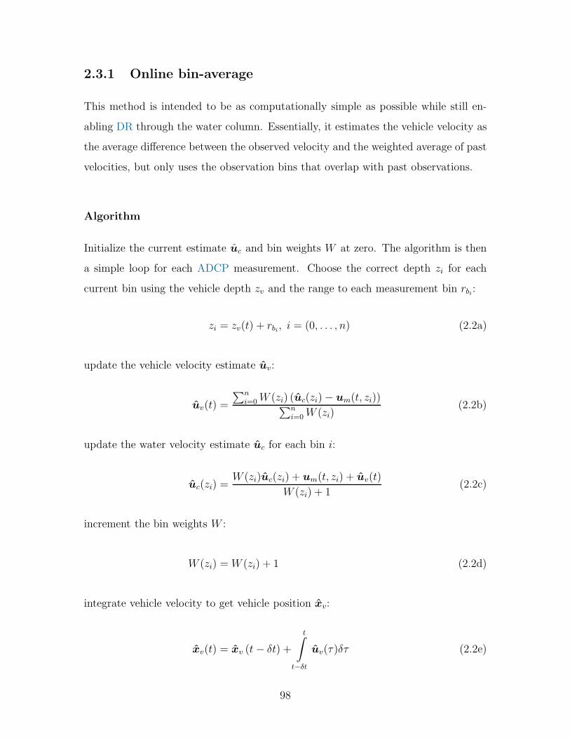
2.3.1 Online bin-average
This method is intended to be as computationally simple as possible while still en-
abling DR through the water column. Essentially, it estimates the vehicle velocity as
the average difference between the observed velocity and the weighted average of past
velocities, but only uses the observation bins that overlap with past observations.
Algorithm
Initialize the current estimate uc and bin weights W at zero. The algorithm is then
a simple loop for each ADCP measurement. Choose the correct depth zi for each
current bin using the vehicle depth zv and the range to each measurement bin rbi:
zi = zv(t) + rbi, i = (0, . . . , n) (2.2a)
update the vehicle velocity estimate uv:
uv(t) =
∑ni=0W (zi) (uc(zi)− um(t, zi))
∑ni=0W (zi)
(2.2b)
update the water velocity estimate uc for each bin i:
uc(zi) =W (zi)uc(zi) + um(t, zi) + uv(t)
W (zi) + 1(2.2c)
increment the bin weights W :
W (zi) =W (zi) + 1 (2.2d)
integrate vehicle velocity to get vehicle position xv:
xv(t) = xv (t− δt) +
t∫
t−δt
uv(τ)δτ (2.2e)
98

Figure 2-2: Current profile and vehicle state estimated by bin-average algorithmin simulation. The solid black line is the truth, and the dashed green line is theestimate. The magenta dotted segments on the current profile represent noisy singlewater profile measurements.
and repeat for each timestep and measurement ensemble. Note that this implementa-
tion uses the vehicle and water velocities in a stationary reference frame (e.g., North,
East, Down), so the measured velocities must be rotated into this stationary frame
using data from the attitude reference.
Simulation
The bin-average approach presented in the previous section was implemented in sim-
ulation using a simple vehicle descent model. The current was restricted to the
x-direction, and modeled as a randomly generated decreasing sinusoid. The vehicle
descended at a rate of 0.27 m/s, and was forced in the x-direction by the current.
The simulation generated ADCP water profile measurements with 1-meter bin size
and zero-mean, σ = 0.13 m/s, random noise.
Figure 2-2a shows that the current profile is identified well, while Figure 2-2b
shows the estimated vehicle velocity follows the actual velocity closely. The actual
and estimated vehicle position are shown in Figure 2-2c. The errors residuals for the
estimated current profile, vehicle velocity, and dead-reckoned position are shown in
99
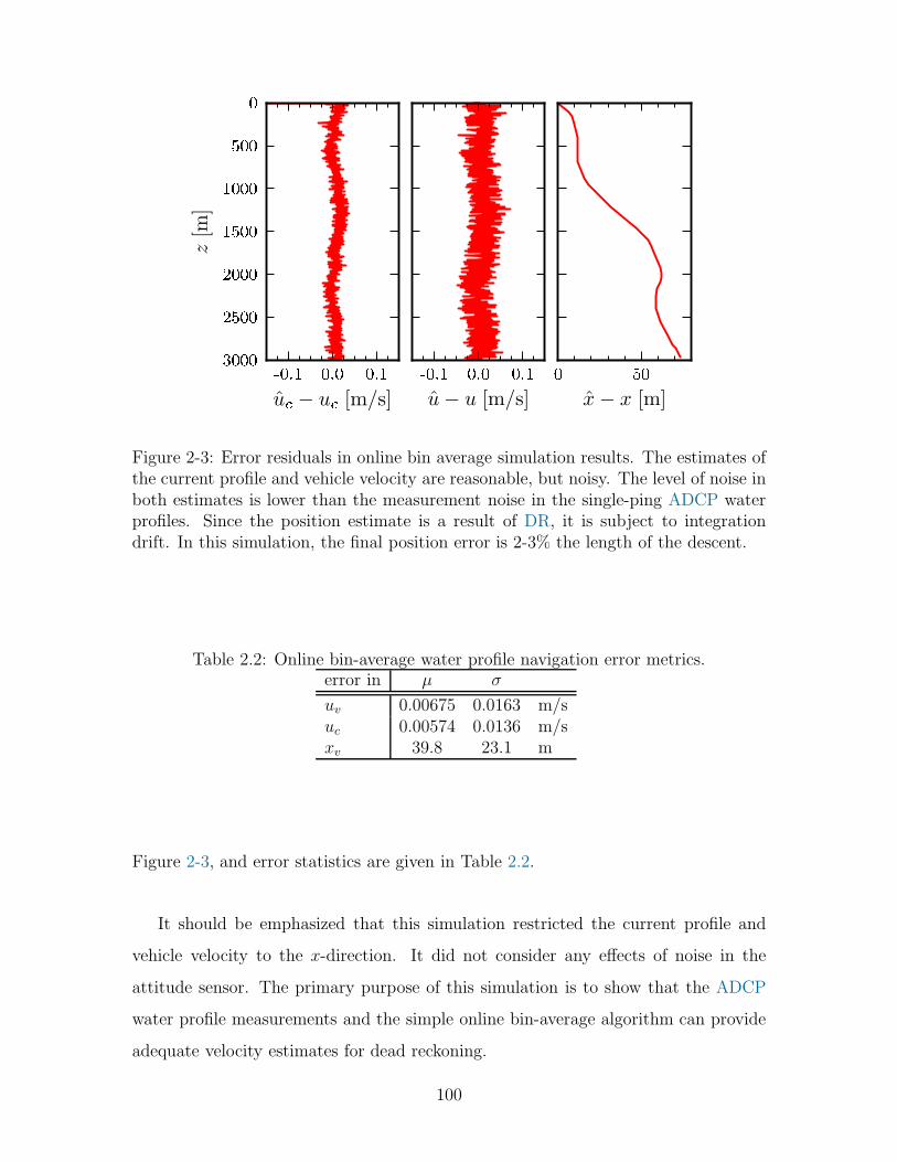
Figure 2-3: Error residuals in online bin average simulation results. The estimates ofthe current profile and vehicle velocity are reasonable, but noisy. The level of noise inboth estimates is lower than the measurement noise in the single-ping ADCP waterprofiles. Since the position estimate is a result of DR, it is subject to integrationdrift. In this simulation, the final position error is 2-3% the length of the descent.
Table 2.2: Online bin-average water profile navigation error metrics.error in µ σ
uv 0.00675 0.0163 m/suc 0.00574 0.0136 m/sxv 39.8 23.1 m
Figure 2-3, and error statistics are given in Table 2.2.
It should be emphasized that this simulation restricted the current profile and
vehicle velocity to the x-direction. It did not consider any effects of noise in the
attitude sensor. The primary purpose of this simulation is to show that the ADCP
water profile measurements and the simple online bin-average algorithm can provide
adequate velocity estimates for dead reckoning.
100

2.3.2 Batch weighted least squares
If the vehicle only needs to localize itself at the end of a water column transit4, the
problem of DR though the water column is essentially equivalent to the LADCP
problem, but focused on the vehicle velocities rather than the current profile. It can
be formulated and solved as a LS or WLS problem [27]:
Ax = b, (2.3)
A
uc(z0)
uc(z1)...
uc(zM)
uv(t0)
uv(t1)...
uv(tN)
=
uwp(t0, z0)
uwp(t0, z1)...
uwp(tN , zM)
ubt(t0)
ubt(t1)...
ubt(tN)
, (2.4)
where b is the concatenation of the water profile measurement ensembles uwp and
bottom track measurement ensembles ubt. The influence matrixA couples the current
profile and vehicle velocities in the solution x to the measurement data. The solution
to this least squares problem minimizes the square of the estimation error:
x = argminx
||b−Ax||2 . (2.5)
In a simple discretized problem with equal bin spacing for the ensembles and the
profile, the influence matrix is sparse and filled by ones and zeros. More generally, the
ensemble and profile bins will have different sizes. The implementation in this paper
computes the influence of each current profile bin on each ensemble water profile bin
based on the distance between the ensemble and profile bin center depths, divided by
4i.e., once it reaches the seafloor after a descent, or once it surfaces after an ascent.
101

the profile bin spacing:
ai,j =1− |ze,i − zp,j|
∆zp(2.6)
This works like a radial basis function with linear interpolation–one might also con-
sider quadratic or Gaussian basis functions. All negative influence coefficients in the
water profile block of the matrix are set to zero, and the sum of each row should be
equal to one.
The upper right block of the influence matrix couples the ensemble water profile
bins to the vehicle motion. Recalling the water profile measurement equation 2.1,
the influence coefficients in this block are negative one wherever the vehicle velocity
maps to an ensemble, and zero otherwise.
For ensembles with bottom track data, the influence matrix is expanded with a
lower block. This is filled with zeros on the left, and a diagonal of negative ones
on the right. The influence coefficients are negative here because the ADCP records
bottom track velocities relative to a stationary instrument.
Figure 2-4 depicts an influence matrix for a simple example with thirteen profile
bins spaced four meters apart. The example shows two measurement ensembles with
four bins spaced at three meters and including bottom track data. The instrument
is at 25 meters when the first ensemble is measured, and 23 meters when it measures
the second.
Once the influence matrix has been set up, the problem can be solved using
normal LS techniques. When one type of measurement is trusted more than another,
WLS should be used. Each measurement is then weighted by the reciprocal of its
standard deviation. (e.g., bottom-track velocities with σ ∼ 0.002 m/s vs. water
profile velocities with σ ∼ 0.02 m/s.)
2.3.3 Recursive least squares
The batch LS method in the previous section is suitable when the vehicle only needs
to know its velocity and position at the end of a water column transit. When the
vehicle needs incremental updates (e.g., for control) a recursive least squares (RLS)
102

−1.0
−0.8
−0.6
−0.4
−0.2
0.0
0.2
0.4
0.6
0.8
1.0
uwp
ubt
uc uv
Figure 2-4: Influence matrix A for a simple system with 13 profile bins spaced 4meters apart, and two measurement ensembles with 4 water profile bins spaced 3meters apart, including bottom track data.
approach is more appropriate. This is also true when the memory available for the
computation is limited, as in a low-power, long range AUV or glider.
Recursive least squares depends on the ability to track an estimate of the state
x and its error covariance P. With this information, an optimal gain can be cal-
culated any time new data is available, without starting the whole calculation from
scratch [56].
The innovation νk in the new data is defined as:
νk = bk −Akxk−1. (2.7)
Given the measurement covariance matrix Rk, the optimal gain can be calculated a
priori:
Kk = Pk−1ATk
(
AkPk−1ATk +Rk
)−1, (2.8)
103

so that the updated state estimate is:
xk+1 = xk +Kkνk, (2.9)
and the updated covariance is:
Pk = (I−KkAk)Pk−1. (2.10)
This form of RLS estimator essentially repeats the measurement update step of the
Kalman filter (KF), without the process update [88]. In signal processing literature,
equation 2.5 is sometimes called the ‘data matrix form’ of the LS estimation prob-
lem [89], so equations 2.7–2.10 can be considered the ‘data matrix form’ of the RLS
filter or estimator.
In this research, the RLS estimator is implemented by initializing a full solution
vector x0 of zeros, and calculating the influence matrix Ak for each measurement
ensemble based on the measured depth of the instrument. An alternate implementa-
tion might only store the instrument velocities at the current timestep, and include a
process update equation–this would produce an augmented state Kalman filter (KF).
2.4 Field Experiences
This section discusses some of the operational and practical challenges involved in
measuring water current profiles from the AUV Sentry. Several field deployments
illustrate lessons learned with respect to ADCP configuration and data quality. We
also present estimated current profiles and dead reckoned vehicle trajectories for each
dive. We compare these estimates to position fixes measured by external acoustic
tracking systems.
104

2.4.1 The AUV Sentry
Sentry is a deep submergence AUV operated by the WHOI DSL. It is the successor
to the autonomous benthic explorer (ABE) [48], with many design improvements to
address the needs of the oceanographic community. Sentry mission tasks include high-
resolution bathymetry, seafloor photography, geomagnetics, and chemical sensing.
Sentry’s navigation sensor suite includes: an INS with fiber-optic gyroscope (IXSEA
PHINS), a 300 kHz DVL/ADCP (Teledyne RD Instruments Workhorse Navigator),
a pressure sensor (Paroscientific Digiquartz), an LBL positioning system (WHOI),
a USBL tracking system (Sonardyne), and a backup magnetic compass (PNI). The
standard science sensor suite includes: a conductivity/temperature probe, precision
magnetometers, a 400 kHz multibeam sonar, and a 12-bit camera. Sentry has also
carried redox potential (eH) probes, dissolved oxygen sensors, an in-situ mass spec-
trometer, a sub-bottom profiler, and sidescan sonar.
Working with multiple sonars
High-resolution bathymetric mapping is one of the primary science tasks for Sentry.
The 400 kHz multibeam sonar collects soundings of the seafloor, which are combined
with vehicle navigation to produce detailed maps for scientists and for joint operations
with other vehicles (e.g., DSV Alvin or ROV Jason).
This presents a minor challenge for DR with the 300 kHz Doppler sonar–the
broadband signal can show up in the multibeam soundings. Careful timing and
a low-latency trigger input allow interleaving so that the multibeam and Doppler
signals do not interfere with each other. However, this also constrains the repetition
rate of both sensors. The nominal sample rate of the sonars is 2 Hz during standard
operations.
Navigated ascent
When configured to measure both bottom track and water profile data, the ADCP
actually uses two different types of pings for each measurement ensemble. The bottom
105

track ping is longer and the seafloor is a reasonably strong acoustic scatterer, so the
ADCP can produce high accuracy velocity measurements at relatively long range.
The length of the water profile ping is limited by the ensemble bin spacing. These
two types of pings are interleaved when the ADCP collects both bottom track and
water profile data. Even if the ensemble has just one ping of each type, this halves
the effective data rate. The bottom-track ping is sent first, and the ensemble data is
reported after the water profile return is received, introducing additional latency.
This lower data rate and measurement latency could potentially degrade the per-
formance of Sentry’s navigation during the main mission, so the data sets for DR
through the water column are currently restricted to the ascent.
Doppler sonar configuration
The ADCP has many parameters that can be adjusted in its firmware. However,
these settings cannot be altered online–the instrument must stop recording data any
time a parameter needs to be changed.
The water profile settings are important for navigating through the water column.
The ADCP is set to record only one ping per ensemble so that it reports data at its
highest rate. The correlation magnitude threshold and echo intensity threshold are
both set to zero so that the ADCP does not throw out any data on its own. This
means that the data will need to be prefiltered before using it for navigation, but it
also ensures that we have the data needed for developing and tuning the navigation
process. The number and spacing of the water profile bins were varied between dives,
and the actual values are noted in the following subsections.
2.4.2 Sentry 059: Galapagos Ridge
Sentry dive 059 was a bathymetry and photography mission on the Galapagos ridge
during the GRUVEE2010 research cruise led by chief scientist John Sinton. At the
end of the mission, Sentry ascended from 1600 meters with an average depth rate
of -0.62 m/s. The ADCP interleaved bottom pings and water pings for the entire
106

0 200 400 600 800
ensemble
0
10
20
30
40
waterprofile
bin
0
30
60
90
120
150
180
210
240
Figure 2-5: Echo intensity from water profile measurements during ascent from Sentrydive 059. Note the bands of slightly increased echo intensity in ensembles 450–850.
ascent. Each ensemble measured 41 water profile bins at a spacing of 2 meters. Low
echo intensity and correlation magnitude, coupled with high error velocity, meant
that much of the data beyond bin 20 was ignored.
Bottom-track interference
Figures 2-5, 2-6, and 2-7 show the echo intensity, correlation magnitude, and error
velocity of the water profile pings from beam 1 at the beginning of the ascent. Signif-
icant interference is visible in ensembles 450 through 850, marked by increased echo
intensity and error velocity, with irregular correlation magnitude.
The ADCP measured these ensembles 6.25–9.5 minutes into the ascent, starting
just after Sentry ascended past 230 meters above the seafloor. This is also at the limit
of the bottom-track range. When it loses bottom-lock, the ADCP begins searching
for the bottom again, but the vehicle continues to ascend and the instrument stays
out of range.
Late returns from bottom track pings are the likely cause of interference in these
ensembles. It is possible that the internal theshold filters of the ADCP, limiting
the range of acceptable correlation magnitude or error velocity, would reduce this
107

0 200 400 600 800
ensemble
0
10
20
30
40
waterprofile
bin
0
30
60
90
120
150
180
210
240
Figure 2-6: Correlation magnitude from water profile measurements during ascentfrom Sentry dive 059. Note the decreased correlation magnitude in near bins (0-10) during ensembles 450–650. The correlation magnitude is increased in outer bins(20-40) for the same timeframe and extending to ensemble 800.
0 200 400 600 800
ensemble
0
10
20
30
40
waterprofile
bin
−1.0
−0.8
−0.6
−0.4
−0.2
0.0
0.2
0.4
0.6
0.8
1.0
Figure 2-7: Error velocity from water profile measurements during ascent from Sentrydive 059. The magnitude of the error velocity is high for almost measurements furtherout than bin 20, and there are bands of incresed error velocity nearer than bin 20 forensembles 450–850.
108

−0.3−0.2−0.10.0 0.1 0.2 0.3
ocean current [m/s]
0
200
400
600
800
1000
1200
1400
1600
dep
th[m
]
North
North
East least squares
East online bin average
−0.4 −0.2 0.0 0.2 0.4
instrument velocity [m/s]
Figure 2-8: Estimated ocean current profile and vehicle velocity during ascent fromSentry dive 059.
interference, but that does not work for this dataset.
Figure 2-8 shows the estimated current profile and vehicle velocity when the in-
put data are limited to those with error velocity less than 0.1 m/s, and correlation
magnitude greater than 72. The online bin average and LS estimates of the north-
ward current and instrument velocity are similar, but the eastward components are
very different in some places. Figure 2-9 plots the resulting vehicle trajectory esti-
mates, with corresponding USBL position fixes for comparison. It seems likely that
the eastward velocities estimated by LS are more correct, but it is also clear that this
dataset does not provide good overall navigation. Later dives used different ADCP
parameters to improve echo intensity and correlation magnitude.
109

−500 −400 −300 −200 −100 0 100
easting [m]
−100
−50
0
50
100
150
northing[m
]
least squares
online bin average
USBL
Figure 2-9: Estimated vehicle trajectory during ascent from Sentry dive 059.
2.4.3 Sentry069: Juan de Fuca
Sentry dive 069 was a 500 meter deep bathymetry mission on Hydrate Ridge during
the ENLIGHTEN10 research cruise led by chief scientist John Delaney. Sentry inter-
leaved bottom pings and water pings for the first 5 minutes of the ascent. There was
a brief data gap while the ADCP was reconfigured to stop collecting bottom track
data. This was an attempt to avoid the possible bottom-track interference encoun-
tered in earlier ascents. Each ensemble measured 21 water profile bins at a spacing
of 3 meters.
Figure 2-10 plots the estimated ocean current profile and instrument velocity
through the ascent. The estimates from batch LS, RLS, and the online bin average
approach are in close agreement. The ADCP data quality for this dive was much
higher, primarily due to the larger ensemble bin spacing, which led to increased echo
intensity and correlation magnitude with decreased error velocities. This comes at
the price of lower spatial resolution, but almost none of the data had to be thrown
out as it had in dive 059.
The integrated vehicle trajectory is shown in figure 2-11. Again, the estimates
provided by the three different approaches are nearly identical. Position fixes from
110

−0.2 −0.1 0.0 0.1 0.2
ocean current [m/s]
0
100
200
300
400
500
dep
th[m
]
North
North
North
East least squares
East recursive least squares
East online bin average
−0.4 −0.2 0.0 0.2 0.4
instrument velocity [m/s]
Figure 2-10: Estimated ocean current profile and instrument velocity during ascentfrom Sentry dive 069. The estimates from batch LS, RLS, and the online bin averageapproach are indistinguishable at this scale on this relatively shallow dive.
111
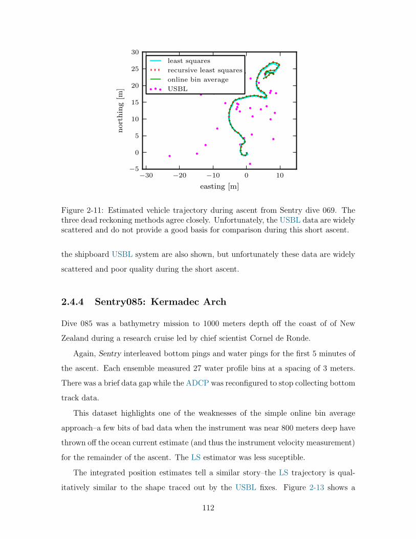
−30 −20 −10 0 10
easting [m]
−5
0
5
10
15
20
25
30
northing[m
]
least squares
recursive least squares
online bin average
USBL
Figure 2-11: Estimated vehicle trajectory during ascent from Sentry dive 069. Thethree dead reckoning methods agree closely. Unfortunately, the USBL data are widelyscattered and do not provide a good basis for comparison during this short ascent.
the shipboard USBL system are also shown, but unfortunately these data are widely
scattered and poor quality during the short ascent.
2.4.4 Sentry085: Kermadec Arch
Dive 085 was a bathymetry mission to 1000 meters depth off the coast of of New
Zealand during a research cruise led by chief scientist Cornel de Ronde.
Again, Sentry interleaved bottom pings and water pings for the first 5 minutes of
the ascent. Each ensemble measured 27 water profile bins at a spacing of 3 meters.
There was a brief data gap while the ADCP was reconfigured to stop collecting bottom
track data.
This dataset highlights one of the weaknesses of the simple online bin average
approach–a few bits of bad data when the instrument was near 800 meters deep have
thrown off the ocean current estimate (and thus the instrument velocity measurement)
for the remainder of the ascent. The LS estimator was less suceptible.
The integrated position estimates tell a similar story–the LS trajectory is qual-
itatively similar to the shape traced out by the USBL fixes. Figure 2-13 shows a
112

−0.2 −0.1 0.0 0.1 0.2
ocean current [m/s]
0
200
400
600
800
1000
dep
th[m
]
North
North
East least squares
East online bin average
−0.4 −0.2 0.0 0.2 0.4
instrument velocity [m/s]
Figure 2-12: Estimated ocean current profile and vehicle velocity during ascent fromSentry dive 085. (RLS estimates are not plotted because they are nearly identicalto the LS.) The online bin average estimated instrument velocity shows an anomalynear 800 meters depth. This highlights a weakness in that method–a few bits of baddata can cascade to throw off the entire estimated ascent.
113

−50 0 50 100 150 200 250
easting [m]
−60
−40
−20
0
20
40
60
northing[m
]
least squares
online bin average
USBL
Figure 2-13: Estimated vehicle trajectory during ascent from Sentry dive 085.
map-view of the ascent trajectory, while Figure 2-14 plots the individual North and
East components.
2.5 Discussion and Conclusions
This chapter has proposed a method for dead reckoning through the water column
using overlapping water profile measurements collected by a vehicle-mounted ADCP.
Field experiences with the deep submervence AUV Sentry, using a 300 kHz ADCP,
have shown that there are some practical challenges to address before this technique is
ready for serious use in autonomous navigation. High data quality must be provided
throughout the entire water column transit–this may be enabled in the future by
adapting ADCP configuration parameters on-the-fly. It would be very advantageous
to be able to avoid the interference from searching for bottom-track by disabling it
without needing to stop water pings.
Although this technique is not quite ready for field service on deep AUVs, it holds
great promise. Dead reckoning using ADCP water profile measurements enhances the
autonomy of underwater vehicles because it enables underwater navigation without
dependence on external systems. It provides a link between GPS at the surface and
114
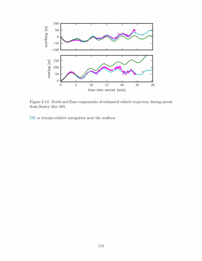
−100
−50
0
50
100
northing[m
]
0 5 10 15 20 25 30
time into ascent [min]
0
50
100
150
easting[m
]
Figure 2-14: North and East components of estimated vehicle trajectory during ascentfrom Sentry dive 085.
DR or terrain-relative navigation near the seafloor.
115

116

Chapter 3
Model-Driven Delayed
Measurement Fusion
Hypothesis
Mathematically rigorous treatment of measurement delays in multi-sensor fusion
Kalman filters can be achieved through state augmentation and conditional time-
varying models without altering the underlying framework.
3.1 Introduction
If a measurement is delayed in time, how should a realtime state estimator process use
the information contained in that measurement to update the current state estimate?
This chapter presents a flexible, model-driven approach to efficiently and effectively
fuse delayed measurements in realtime. The specific motivation for this study is
acoustic position aiding for underwater navigation.
Efficiency and effectiveness are two important properties for a realtime state es-
timator. In this context, efficiency means that the fusion process should avoid dupli-
cated effort (i.e., repeated computations) whenever and wherever possible. We also
want to avoid increasing the dimension of the problem (i.e., the length of the state
vector) any more than necessary. We only want to carry enough extra information to
117

fuse the delayed measurement in a principled manner, and leave behind any informa-
tion we won’t use. Effectiveness means (at least) that fusing a delayed measurement
should reduce the uncertainty in the state estimate. It can also relate to the ease of
operating and designing the filter. The model-driven approach presented here handles
delayed measurements more efficiently and effectively than previous methods.
The remainder of this section introduces the general problem in more detail. Sec-
tion 3.1.1 outlines the common methods for measuring position underwater, and goes
into more detail on two acoustic tracking methods that will serve as application ex-
amples for the proposed delayed measurement fusion approach. Section 3.1.2 briefly
reviews related work, and section 3.1.3 enumerates the contributions of this research.
We classify and briefly discuss different types of measurement delays in section 3.2.
We present the details of model-driven delayed measurement fusion in section 3.3,
reviewing some key concepts of the Kalman filter before proposing two specific modi-
fications to compensate for measurement delay. Section 3.4 walks through a canonical
example, using a damped harmonic oscillator with delayed position measurements to
illustrate the process proposed here.
Then we apply the proposed model-driven delayed measurement fusion approach
to the real-world problem of underwater navigation. We present ultra-short baseline
(USBL)-aided dead reckoning (DR) as a loosely coupled example in section 3.5, and
long baseline (LBL)-aided DR as a more tightly integrated example in section 3.6.
Both examples are demonstrated on field data from the National Deep Submergence
Facility (NDSF) autonomous underwater vehicle (AUV) Sentry.
3.1.1 Delayed measurements in underwater positioning
For oceanographic underwater vehicles, it is as important to know the location where
measurements or samples were collected as it is to collect the data in the first place.
Localization is also important in most military and offshore industry applications.
After all, knowing where you are is often the first step in getting where you need to
be.
Precise, robust underwater navigation relies on many measurements, fused in an
118

intelligent way, to produce an accurate state estimate. Realtime navigation relies
on DR–measuring vehicle orientation with a compass or gyrocompass and measuring
vehicle velocity with a Doppler velocity log (DVL) or estimating it from a dynamic
model. This is essentially integrating the first-order kinematics of the vehicle forward
in time. Inertial navigation integrates forward from the second-order kinematics–
using accelerometers to measure acceleration, and gyroscopes to measure angular
rates. These are both attractive options because they require no external infrastruc-
ture and can operate at high update rates. However, without position measurements,
any inertial navigation or dead reckoning system will accumulate error and uncertainty
over time. Including position aiding makes the navigation solution more accurate and
robust in the long term.
Since the radio frequency signals of Global Positioning System (GPS) do not
penetrate the ocean surface, underwater navigators must rely on other means to
determine position. Depth is determined from measurements of pressure, tempera-
ture, and conductivity [2]. Long baseline (LBL), short baseline (SBL), or ultra-short
baseline (USBL) acoustic positioning systems provide measurements in the North-
East plane. More recently, terrain-relative techniques using bathymetry and/or pho-
tography have been developed to provide relative position measurements [38, 45, 90]
for navigation aiding.
The methods summarized above all provide relative position information in the
local navigation frame. They must be geo-referenced to provide positions in the global
frame: LBL beacons must be surveyed, SBL and USBL systems must be coupled to
GPS and attitude sensors, and terrain-relative navigation must be over known terrain
or have known boundary conditions.
With the exception of depth measurements, all of these methods for determining
position have inherent latency. There is a finite delay between the time a measure-
ment is valid and the time it is available. The delays associated with (x, y) position
measurements underwater are on the order of seconds, and in some cases longer. It
is important to understand these delays, and properly account for them, in order to
achieve precise and robust navigation.
119

3.1.2 Related Work
The Kalman filter
The Kalman filter (KF) [91] is an optimal recursive estimator for a linear system with
stochastic inputs. It fuses state measurements of a system with estimates provided
by a model of that system in proportion to the covariances of the measurements and
the estimates. Many implementations use simple kinematic process models to provide
state estimates. The KF has been continually expanded, modified, and re-explained
in the past 50 years. A good introduction to Kalman filtering methods is given in [88].
The extended Kalman filter for nonlinear systems
The Extended Kalman filter (EKF) is a generalization of the Kalman filter to deal
with nonlinear systems. It linearizes the system at the current estimated state, then
analytically propagates a Gaussian random variable through the linearized transition
equations. Although this process can be complicated, the EKF is the de facto stan-
dard for many estimation applications. It has been widely applied to AUVs, both as
a real-time estimator (e.g., [92]) and as a postprocessing filter-smoother (e.g., [49]).
It is also used in many of the single-range LBL systems mentioned in section 0.2.1.
Sigma point Kalman filters for nonlinear systems
Julier and Uhlmann introduced the unscented transform (UT) as a new approach to
pass important statistics of a random variable through a general nonlinear transfor-
mation [93–95]. It was extended to the unscented Kalman filter (UKF) for filtering
nonlinear systems in [96, 97]. It has since been shown to outperform the extended
Kalman filter (EKF) in many situations [96–98].
The UKF has been classified as an example of sigma point filtering [99–101]. The
sigma point approach uses a weighted, deterministic sampling scheme to propagate
estimated error through nonlinear system dynamics. This is essentially a formalism
to perform weighted statistical linear regression (WSLR) as a random variable passes
through many general transformations. It provides improved performance in highly
120

nonlinear systems, and does not require analytical derivation of Jacobians for the
process model. This makes it attractive in a ‘black-box’ sense, and should simplify
its application to a coupled nonlinear system like an underwater vehicle.
Handling delayed measurements
The simplest way to deal with a measurement delay is simply to ignore it and fuse
the measurement as if it is an observation of the system state at the current instant.
This is the standard approach, but if the delay is significant it will produce inaccurate
estimates. A brute force approach would recalculate the state estimates over the entire
delay interval after the measurement arrives. This would provide accurate estimates,
but at increased computational cost. Depending on the length of the delay, this
approach can become impractical or untractable. Here we will review some more
principled methods to account for the delay.
State augmentation is a standard method to handle situations where the current
state of a system is correlated to another variable–including its past state. This
has been applied to linear systems with single or multiple delays (e.g., [102]). Used
carefully, state augmentation can enable a KF to handle delayed measurements.
Leonard & Rikoski use an EKF with augmented states representing the past tra-
jectory of a mobile robot in [103]. These augmented states are used in feature ini-
tialization for concurrent mapping and localization–enabling the robot to use data
from multiple timesteps for improved data association and decision making. In [104],
Rikoski applies this approach to handle time-of-flight measurements in LBL acoustic
positioning for an underwater vehicle1. The augmented state includes the full state
at the instant the robot interrogates the net, as well as the full state at the instant it
receives the reply from each transponder.
Ridao, et al.use a bounded circular buffer of past poses2 to fuse USBL position
1Section 3.6 explores a similar application–formulated independently of Rikoski’s work–using themodel-driven delayed measurement fusion approach presented in this chapter for LBL-aided DR.
2Since the delayed USBL measurements only relate to the position of the remotely operatedvehicle (ROV) and not its velocity, Ridao, et al.use the 4-element pose vector for each augmentedstate, instead of the full 8-element state vector. This reduces the dimension of the filter–and savessome computation cost–but still uses more resources than strictly necessary.
121

measurements with DR based on an attitude and heading reference system (AHRS)
and a DVL in [105]. They assume that the clocks of the USBL system and the vehicle
are synchronized3, and validate the method using a tethered ROV. This approach
has the advantage that it imposes an upper limit on the growth of the state and filter
dimension. To ensure the appropriate state will be in the buffer when the delayed
measurement arrives, the buffer must include all past poses up to the maximum delay
length–this increases the dimension of the filter and the computation cost. For this
approach to work, the bounded circular buffer must always contain more past vehicle
poses than the fusion step of the filter requires–so by definition, this implementation
uses more resources than necessary.
To reduce this extra cost, Challa suggests a variable dimension augmented state
KF in [102]. Instead of storing all the past states over the entire delay interval, this
filter adaptively augments only the essential past states–the ones that the delayed
measurement will observe4. This results in a more efficient filter with comparable
estimation accuracy.
Approaching the problem from a different direction, some researchers use a stan-
dard KF formulation during the delay interval, then calculate a different correction
term when fusing the delayed measurement.
Hilton, et al. apply this to tracking problems with time-delayed measurements
in [106]. Assuming constant-velocity tracking, they back-propogate the state estimate
through linearized system dynamics to the instant the delayed measurement was valid.
They then minimize the trace of the covariance to solve for a modified Kalman gain.
Simulations showed that this approach outperformed several ad-hoc methods, and
nearly recovered the performance of a filter with no delay in its measurements.
In [22, 78], Farrell uses an error state EKF for sensor fusion aboard an AUV–
aiding an inertial navigation system (INS) with velocity measurements from a DVL,
3This restriction is not necessary if the USBL system can report the time it is interrogated, seesection 3.5.
4Although Challa’s work does not investigate measurements that are composite observations ofthe state at two distinct instants, the variable dimension augmented state KF has a similar delaytreatment to Rikoski [104]. This variable dimension approach is also similar to the work by van derMerwe, et al., which is discussed later in this section.
122

heading measurements from a magnetometer, depth measurements from a pressure
sensor, and two-way travel time measurements from four LBL transponders5. The
measurement delay compensation uses a wait-and-correct strategy. Any time the
vehicle interrogates the LBL net, the error state accumulates until the end of that
LBL measurement cycle. In the meantime, navigation relies entirely on the INS–
measurements from other aiding sensors are not fused during the delay interval. This
effectively reduces the aiding rate to the rate of the slowest sensor–including mea-
surement delays. While this approach may be suitable for a system with high quality
inertial navigation, it may not perform well on a system with a low-grade INS, and
is not directly applicable to any system without inertial sensing.
Alexander proposed an approach in [107] where a correction term was added to
the estimates of a linear KF once the delayed measurement was available. The covari-
ance, however, was updated early, when the measurement should have been valid–this
resulted in sub-optimal fusion of any measurements during the delay interval. Larsen,
et al., reformulated this approach in [108] to make it easier to implement. That study
also suggested a two-filter method to optimally fuse all measurements, with or with-
out delay. This modified two filter method achieved the same low estimation error
as brute-force recalculation, but at reduced computational cost. It was applied to
vision-aided navigation for an autonomous unmanned ground vehicle (UGV) in [109].
van der Merwe, et al. adapted Larsen’s two-filter method to nonlinear systems
using a sigma point Kalman filter (SPKF) with augmented states instead of separate
filters6 [99–101], bringing the ‘filter and correct’ approaches back to state augmenta-
tion. This delayed-state SPKF was applied to navigate an autonomous helicopter un-
manned aerial vehicle (UAV) with fast dynamics and a slow GPS receiver. Although
5The LBL measurement equation in [22, 78] deals with the fact that a two-way travel time isa composite observation of the vehicle state at two distinct instants by back-propogating the stateestimate at the reply instant through linearized vehicle kinematics to the interrogation instant.
6Although delay compensation can be achieved with state augmentation, care must be takenwhen initializing or updating the augmented states. The method given in equations 5.63 and 5.64of [99] produces a covariance matrix with four identical blocks–this is guaranteed to be singular.The model-driven delayed measurement fusion method presented in this chapter avoids this issue byusing appropriate time-varying conditional process models to initialize and update the augmentedstates.
123

the delay was only on the order of 50 ms, compensating for it reduced estimation
error in position, velocity, and attitude.
3.1.3 Contributions
The method proposed in this chapter is an efficient, flexible, and mathematically prin-
cipled approach to delayed measurement fusion. It is based on state augmentation–
adding only the minimal amount of extra memory necessary to deal with delays. It
works entirely within the KF framework–using time-varying conditional models to
manage the augmented states–separating the user from any external or ad hoc ad-
justments to the state estimate or filter covariance.
Table 3.1 compares the model-driven approach to other related work in the litera-
ture. The main points are the minimal increase in dimension and the ability to work
entirely within a single KF. It should work with any7 kind of KF, and is demonstrated
here using the classical KF for linear systems and the SPKF for nonlinear systems.
The previous literature that includes delay compensation can be loosely divided
into methods using state augmentation, and methods that use an external process to
back-propogate or wait-and-correct. For a filter with an original state dimension N ,
the state augmentation approaches use a filter of dimension 2N to handle the delay8.
The external processes in the other methods also have calculations on the order of
N , for an effective dimension ∼ 2N . The model-driven approach proposed here, on
the other hand, produces a filter with dimension N +M , where M is the dimension
of the delayed measurement, and usually M < N .
Many of these approaches can be extened to deal with multiple delayed measure-
ments. This ability comes with additional increase in dimension, associated with D,
the number of delayed measurements. The numbers in Table 3.1 denote this ad-
ditional cost only for work where support for multiple delayed measurements was
demonstrated.
7including an EKF, although that has not been demonstrated here and remains for future work8Ridao uses a filter with dimension N +LP , where L is the maximum delay length, and P is the
dimension of a reduced state (the pose). In practice, the maximum delay length may be very large,so even though P < N , LP is likely greater than N , and the total filter dimension is N +LP ≫ 2N .
124
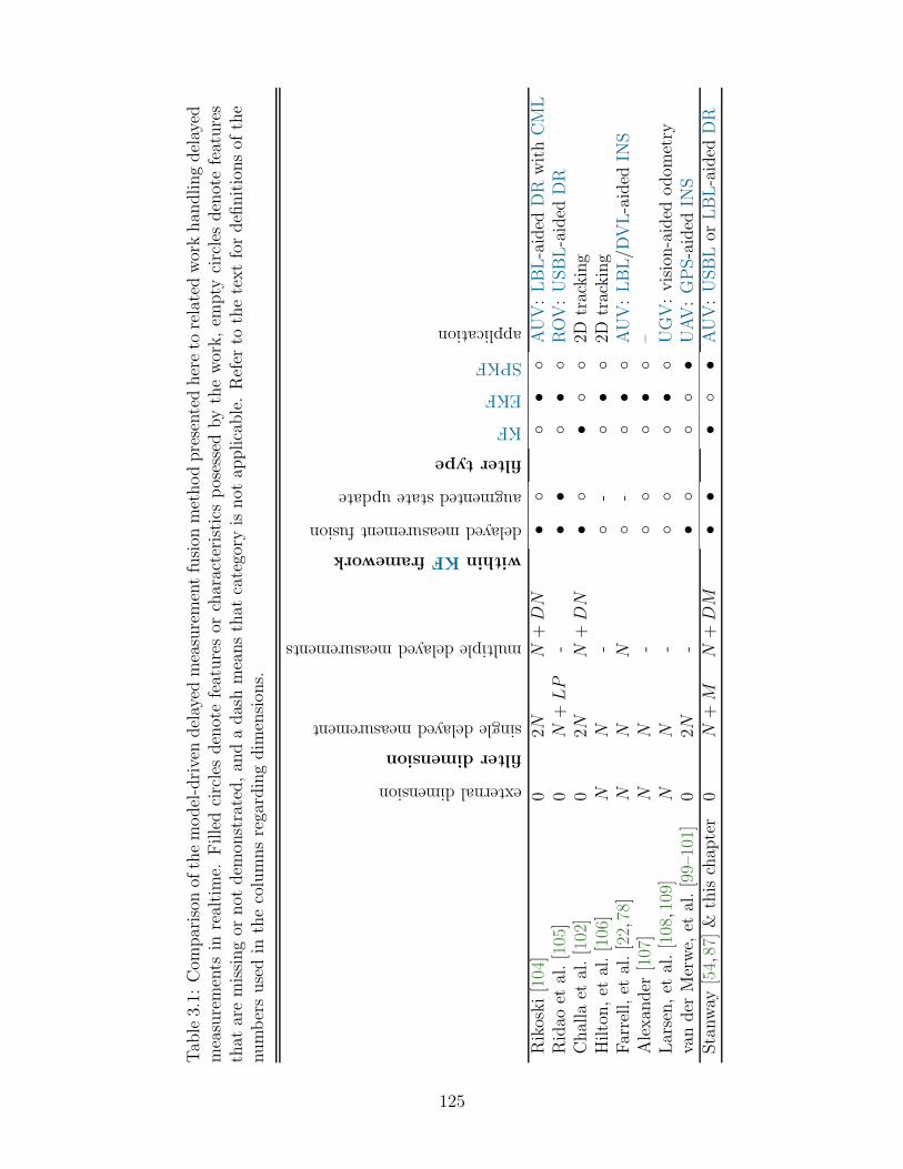
Tab
le3.1:
Com
parison
ofthemodel-drivendelayed
measurementfusion
methodpresentedhereto
relatedworkhan
dlingdelayed
measurements
inrealtime.
Filledcirclesdenotefeaturesor
characteristicsposessedbythework,em
pty
circlesdenotefeatures
that
aremissingor
not
dem
onstrated,an
dadashmeansthat
category
isnot
applicable.Refer
tothetextfordefinitionsof
the
numbersusedin
thecolumnsregardingdim
ension
s.
externaldimension
filterdimension
singledelayedmeasurement
multipledelayedmeasurements
withinKFframework
delayedmeasurementfusion
augmentedstateupdate
filtertype
KF
EKF
SPKF
application
Rikoski[104]
02N
N+DN
•
•
AUV:LBL-aided
DR
withCML
Ridao
etal.[105]
0N
+LP
-•
•
•
ROV:USBL-aided
DR
Challa
etal.[102]
02N
N+DN
•
•
2D
tracking
Hilton,et
al.[ 106]
NN
-
-
•
2Dtracking
Farrell,et
al.[ 22,78]
NN
N
-
•
AUV:LBL/D
VL-aided
INS
Alexan
der
[107]
NN
-
•
–Larsen,et
al.[108,109]
NN
-
•
UGV:vision-aided
odom
etry
vander
Merwe,
etal.[99–101]
02N
-•
•
UAV:GPS-aided
INS
Stanway
[54,87]&
thischap
ter
0N
+M
N+DM
••
•
•AUV:USBLor
LBL-aided
DR
125

The methods relying on external processes have the additional downside that
they are not integrated into the filter structure, and therefore less portable to other
applications and other types of KF (e.g. SPKFs for nonlinear systems.)
The approach presented here handles delayed measurements in a mathematically
principled way with a modest increase in filter dimension (and associated compu-
tational complexity). Its flexibility allows it to be applied to linear or nonlinear
systems, in synchronous or asynchronous filters. The next few sections will show how
the model-driven approach makes delay treatment simple for the user reduces error
and uncertainty in state estimates.
3.2 Types of measurement delay
Any single measurement may be subject to several distinct delays of different types:
physical, communications, hardware/firmware, and processing.
Physical delays are governed by the laws of nature. One example is the travel time
delay for an electromagnetic or acoustic wave. Little can be done to reduce physical
delays without changing operations–minimizing the distance to acoustic beacons, for
example. These delays are negligible in some cases (e.g. GPS localization of an auto-
mobile), but significant in others (e.g. long-range LBL localization of an underwater
vehicle).
Communications delays are primarily due to network latency. This means they
overlap a bit with physical delays, but they also include delays from dropped packets
or incomplete feedback.
Hardware and firmware delays are often included to protect equipment and en-
sure reliable operation. Examples include the blanking time an acoustic transceiver
waits before listening for a return, and the turn around time a transponder waits
before sending a reply. These delays usually have recommended values and limited
adjustability.
Finally, processing delays are dictated by the complexity of the problem and the
algorithm used to solve it. Much can (and has) been done to minimize this type of
126

delay in modern systems, and computers are only getting faster. However, embedded
devices with limited processing power can still impose non-negligible delays. This was
the case in the first application of a SPKF to a delayed measurement problem [100,
101].
3.3 Model-driven delayed measurement fusion
This section proposes a new, entirely model-based, approach to delayed measurement
fusion. This flexible approach can treat multiple delayed measurements with lengths
that vary in time–it can even handle measurements with multiple delays. Perhaps
most importantly, this approach handles delayed measurements in a mathematically
principled fashion without changing the underlying structure of the KF framework.
This section presents the theory behind model-driven delayed measurement fusion.
We begin by reviewing the underlying KF framework and the key concepts behind it.
Then we carefully define the nomenclature and notation for the timeline of delayed
and undelayed measurements. Then we show how state augmentation can be used to
store the necessary information for delayed measurement fusion. Then we show how
conditional, time-varying process and measurement models can be used to manage the
augmented states and delayed measurements without changing the KF framework.
The next section will walk through an example application using a damped harmonic
oscillator.
3.3.1 Timeline and nomenclature for delayed measurements
Before diving into the details of delayed measurement fusion, it will be helpful to
take a moment and carefully define our reference frame and nomenclature. Data
from several different instants of time are used, so it is important to orient ourselves
and be consistent.
Consider the relevant instants in time looking back from the time of fusion, as
illustrated in Figure 3-1:
127
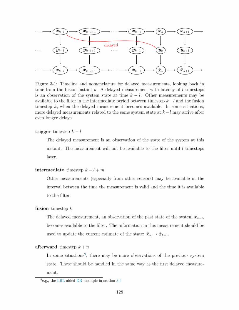
· · · xk−l xk−l+1 · · · xk−1 xk xk+1
· · · yk−l yk−l+1 · · · yk−1 yk yk+1
· · · xk−l xk−l+1 · · · xk−1 xk xk+1
delayed
Figure 3-1: Timeline and nomenclature for delayed measurements, looking back intime from the fusion instant k. A delayed measurement with latency of l timestepsis an observation of the system state at time k − l. Other measurements may beavailable to the filter in the intermediate period between timestep k− l and the fusiontimestep k, when the delayed measurement becomes available. In some situations,more delayed measurements related to the same system state at k− l may arrive aftereven longer delays.
trigger timestep k − l
The delayed measurement is an observation of the state of the system at this
instant. The measurement will not be available to the filter until l timesteps
later.
intermediate timestep k − l +m
Other measurements (especially from other sensors) may be available in the
interval between the time the measurement is valid and the time it is available
to the filter.
fusion timestep k
The delayed measurement, an observation of the past state of the system xk−l,
becomes available to the filter. The information in this measurement should be
used to update the current estimate of the state: xk → xk+1.
afterward timestep k + n
In some situations9, there may be more observations of the previous system
state. These should be handled in the same way as the first delayed measure-
ment.
9e.g., the LBL-aided DR example in section 3.6
128

Alternately, looking forward from the instant that the measurement observes the
system, the relevant timestps are k, k+m, k+ l, k+ l+ n. The dummy indices m,n
will change as the system and filter state evolve. They help provide precise notation,
but may never be explicitly tracked or used by the filter. The latency l may not be
constant, or even explicitly known.
With this nomenclature in mind, we can discuss the KF framework and propose a
specific method for dealing with delayed measurements without altering that frame-
work.
3.3.2 The Kalman filter framework
Our goal is to effectively and efficiently fuse delayed measurements into the current
state estimate of a dynamic system. To encourage understanding and simplify expo-
sition, we will begin with a linear discrete state space model (DSSM).
xk+1 = Akxk +Bkuk +Gkvk (3.1)
yk = Ckxk +wk (3.2)
The system state xk is driven by the known control input uk and the unknown
process noise vk ∼ N (0,Qk). Observations yk are a function of the current state,
with random measurement noise wk ∼ N (0,Rk).
Given these observations, the Kalman filter (KF) provides an optimal estimate of
the system state. Many different derivations exist, see for example [88, 91].
The KF is often presented in two steps: predict and update. The prediction step
computes a priori estimates of the state, its covariance, and the observation:
x−k+1 = Akx
+k +Bkuk (3.3a)
P−k+1 = AkP
+k A
Tk +Qk (3.3b)
yk+1 = Ckx−k+1 (3.3c)
129

Adjusting the prediction: innovations
The first key concept of KFs is the innovation–this is simply the difference between
predicted and observed measurements of the system state:
yk = yk − yk, (3.4)
this is also called the measurement residual. In the KF framework, the filter doesn’t
really care about the exact value of any given measurement–it really only wants to
know how far off the prediction was–this is the key that will enable us to handle
measurements with delays. The update step of the KF applies the optimal gain to
the innovation to compute a posteriori estimates of the state and covariance:
x+k = xk +Kk (yk − yk) (3.5)
P+k = (I−KkCk)P
−k , (3.6)
which brings us to the second key concept: the optimal Kalman gain.
The optimal Kalman gain: a ratio of uncertainties
Given a state estimate with some quantified uncertainty and an observation of that
state with some other uncertainty, an optimal approach to fuse these two bits of
information is to weight them by the ratio of uncertainties. This is the approach used
in the KF framework.
A minimum mean-squared error (MMSE) derivation of the KF (e.g., [99]) gives
the Kalman gain [97, 101]:
Kk = P−xkyk
(
P−ykyk
)−1(3.7a)
where x−k , y
−k are the residuals of the a priori estimates of the state and the observa-
tion, and their (cross-) covariances are P−xkyk
,P−ykyk
.
130
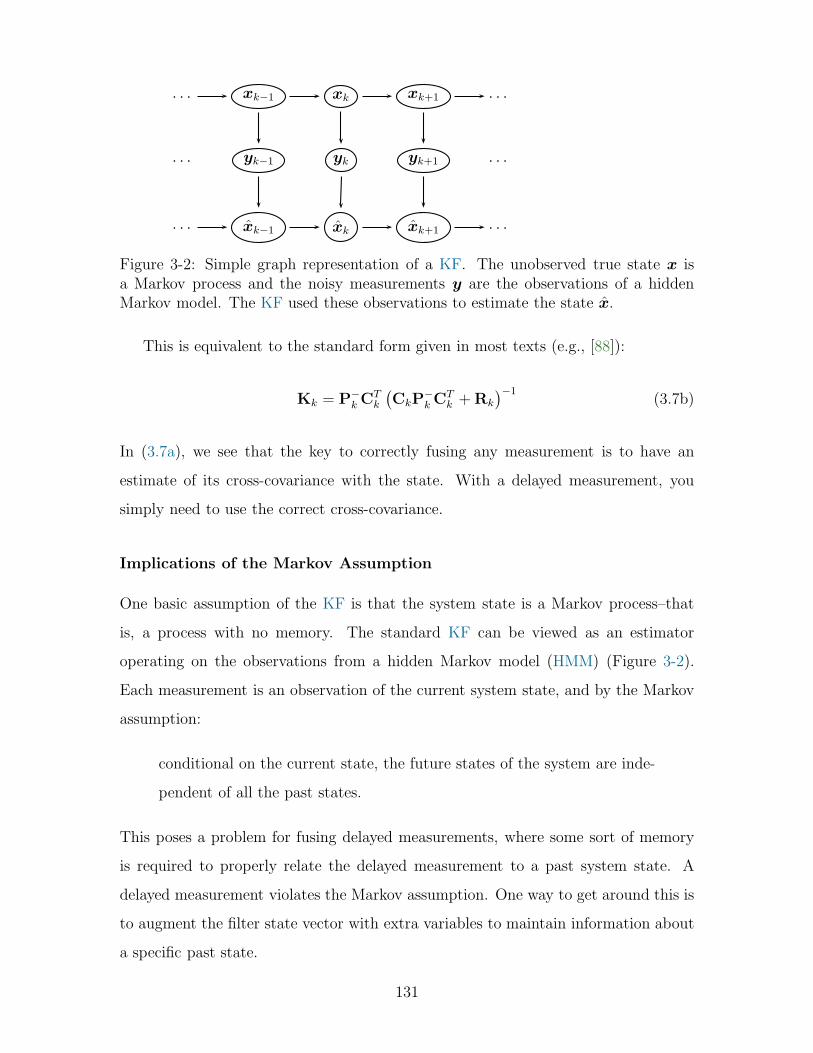
· · · xk−1 xk xk+1 · · ·
· · · yk−1 yk yk+1 · · ·
· · · xk−1 xk xk+1 · · ·
Figure 3-2: Simple graph representation of a KF. The unobserved true state x isa Markov process and the noisy measurements y are the observations of a hiddenMarkov model. The KF used these observations to estimate the state x.
This is equivalent to the standard form given in most texts (e.g., [88]):
Kk = P−k C
Tk
(
CkP−k C
Tk +Rk
)−1(3.7b)
In (3.7a), we see that the key to correctly fusing any measurement is to have an
estimate of its cross-covariance with the state. With a delayed measurement, you
simply need to use the correct cross-covariance.
Implications of the Markov Assumption
One basic assumption of the KF is that the system state is a Markov process–that
is, a process with no memory. The standard KF can be viewed as an estimator
operating on the observations from a hidden Markov model (HMM) (Figure 3-2).
Each measurement is an observation of the current system state, and by the Markov
assumption:
conditional on the current state, the future states of the system are inde-
pendent of all the past states.
This poses a problem for fusing delayed measurements, where some sort of memory
is required to properly relate the delayed measurement to a past system state. A
delayed measurement violates the Markov assumption. One way to get around this is
to augment the filter state vector with extra variables to maintain information about
a specific past state.
131

3.3.3 Maintaining the delayed innovation and cross-covariance:
state augmentation
State augmentation expands the filter dimension to include extra information (in this
case, related to a specific system state in the past.) This additional information a is
concatenated to the original state x to produce the augmented state vector xa:
xa =
x
a
(3.8)
=[
x1 x2 · · · xM | a1 a2 · · · aL
]T
(3.9)
van der Merwe, et. al. used this approach in [99–101] to fuse latent GPS mea-
surements of the position of a helicopter UAV. In that study, the augmented states
included a full copy of the original state vector, here we employ a subtly different
approach.
Delayed innovation
We specifically use a priori estimates of future measurements as augmented states.
At the trigger instant:
xak =
xk
y−k+m
(3.10)
or at the fusion instant
xak =
xk
y−k−l
(3.11)
This maintains all the information necessary to fuse the delayed measurement later.
And, it keeps the filter dimension small10–this is important for realtime operations on
10Using a priori estimates of future measurements as the augmented states ensures a near-minimalincrease in filter dimension. In some specific cases (e.g., overconstrained LBL with more than 4transponders) the dimension could be mildly decreased further. The difference is small compared
132

a wide variety of platforms, or if the KF is the kernel of a more intensive process (e.g.,
to update the particles in a particle filter). This approach also pre-computes so that
the innovation can be calculated immediately and the processing delay of the filter
itself is minimized. A more subtle advantage is that it helps ensure that the filter
remains stable–introducing the measurement noise into the augmented covariance
(detailed in the next section) helps keep it from becoming singular.
Cross-covariances
The full augmented covariance matrix Pa−k is:
Pa−k =
Px−
kx−
kP
x−
ky−
k+m
Py−
k+mx−
kP
y−
k+my−
k+m
. (3.12)
It contains the original covariance matrix Pxkxk, the covariance of the delayed
innovation Py−
k+my−
k+m, and the cross-covariances between them P
x−
ky−
k+m= PT
x−
ky−
k+m
.
Recalling (3.7a), we see that the augmented covariance matrix maintains all the
information necessary to fuse the delayed measurement.
3.3.4 Driving the new filter: time-variant conditional process
and measurement models
As mentioned earlier, an augmented state means process and measurement models
need to be adjusted anyway–why not use this to our advantage and define these
models to handle the augmented states and delayed measurements without any ad-hoc
adjustments to the filter?
Trigger process model
The filter needs a way to choose between different process models. In the examples
of this chapter, the trigger is obvious and can be provided by the system–in other
to storing the full past state as in [99–101], or multiple past states as in [105] or a pose graphimplementation.
133

cases, one might have to use additional augmented states to estimate the time of the
trigger condition.
The trigger process model is always the same. The first part is simply the original
process model. The second part is the measurement model for the (expected) delayed
measurement. This is flexible enough to work with many kinds of systems, but specific
enough to ensure both the original and augmented states are updated properly.
The measurement error covariance matrix should be added11 to the augmented
state covariance, just as if it were a regular measurement.
Loosely-Coupled Measurements
In this case, the delayed measurement is some direct (linear) function of state(s). An
example would be a USBL system that provides a fully-computed geographic position
fix.
The augmented state is the a priori estimate of the delayed measurement, so the
delayed innovation is straightforwarrd:
yk = yk − y−k (3.13)
= yk −Cselectk xa
k− (3.14)
where Cselectk is simply a matrix of ones and zeros that selects the appropriate entry
in the augmented state vector.
Tightly-Coupled Measurements
This approach involves a more complex measurement model. For example, the full
interrogation-response time for a particular transponder in an LBL net.
In this case, the delayed measurement may combine several augmented states (i.e.,
from multiple delays) or may combine delayed and undelayed information:
yk = yk −(
Cselectk xa−
k + hundelayed(xa−k )
)
(3.15)
11or equivalently treated, if the measurement noise is not strictly additive
134

We will revisit this kind of measurement in section 3.6.
3.4 A canonical example:
the damped harmonic oscillator
We introduce the model-driven delayed measurement fusion approach using a simple
one-dimensional system, showing the natural progression from the standard KF to
our new delayed measurement filter. Along the way, we use simulations to study the
behavior of a KF without delayed measurements, a KF with delayed measurements
that ignores the delay, and the new filter that compensates for measurement delays.
We also use this example to discuss an alternative ad-hoc approach to compensate
for measurement latency.
3.4.1 System Dynamics
The dynamics of a generalized damped harmonic oscillator (DHO) are described by
the second-order differential equation:
ξ(t) + 2ζωnξ(t) + ω2nξ(t) = u(t) + v(t), (3.16)
where ζ is the damping coefficient, ωn is the natural frequency, u(t) is a known control
input signal, and v(t) is an unknown environmental disturbance. For this example,
we will assume zero control:
u(t) = 0 ∀ t, (3.17)
and mutually uncorrelated additive white Gaussian process noise:
v(t) ∼ N (0, σv) , E [v (t1) v (t2)] = 0 ∀ t1 6= t2. (3.18)
This simple system may not be intellectually stimulating when taken alone, but
135

its simplicity makes it ideal for illustrating the progression of methods for fusing more
complex types of measurement sequences with and without delay.
If the system is a point mass connected to a linear spring and damper, the gener-
alized variable ξ represents position, ξ is velocity, and ξ is acceleration.
3.4.2 Discrete State Space Model
The system dynamics (3.16) are written in state space form as:
x1
x2
=
0 1
−ω2n −2ζωn
x1
x2
+
0
1
v (3.19)
where x1 = ξ, and x2 = ξ.
Direct Euler integration12 gives an approximate DSSM for the dynamic process:
ξk+1
ξk+1
≃
1 ∆t
−ω2n∆t 1− 2ζωn∆t
ξk
ξk
+ vk (3.20a)
xk+1 = Axk + vk (3.20b)
This process model predicts the future state, given the current state.
3.4.3 Full measurements
Now assume that the system has sensors to measure its position ξ and velocity ξ.
Both measurements are corrupted by mutually uncorrelated additive Gaussian white
noise:
w ∼ N (0,R) , R =
σw10
0 σw2
(3.21a)
E[
(wi) (wj)T]
= 0 ∀ i 6= j (3.21b)
12For continued simplicity, we use Euler integration to move from continuous to discrete time.This is also known as a zero-order-hold approach. Alternative approaches, for example using Tustin’smethod (bilinear interpolation), or the exact matrix exponential, may prove valuable in future studiesof delayed measurement fusion.
136

The filter receives instantaneous measurements from both sensors at each timestep.
This direct13 measurement model is:
y1
y2
=
1 0
0 1
ξ
ξ
+
w1
w2
(3.22a)
yk = Cxk +wk, (3.22b)
3.4.4 Fusing measurements with different sampling periods
In many practical applications, engineers need to fuse multiple types of measurements,
each with different sampling frequencies. To enable this, we must make a slight
modification to the standard KF problem presented above.
The physical system has not changed, so the process model (3.20) stays the same.
However, the measurement system has changed, so the measurement model (3.22b)
must also change to reflect this.
Measurement Selection Matrix
In a linear (or linearized) system, we can simply pre-multiply the measurement matrix
by a selection matrix:
yk = Cselectk Cxk +wk. (3.23)
The selection matrix is a matrix of ones and zeros. It varies in time so that (3.23)
generates the appropriate a priori measurement estimates to compare with the actual
measurements.
For example, at discrete time instant k, the velocity sensor provides a measure-
ment, but the position sensor does not. In this case, the selection matrix would
13Again, a direct measurement model may not be the most intellectually stimulating, but it servesour purposes well here. We will consider a more complex type of measurements in the LBL-aidedDR example in section 3.6.
137
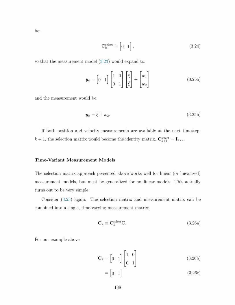
be:
Cselectk =
[
0 1]
, (3.24)
so that the measurement model (3.23) would expand to:
yk =[
0 1]
1 0
0 1
ξ
ξ
+
w1
w2
(3.25a)
and the measurement would be:
yk = ξ + w2. (3.25b)
If both position and velocity measurements are available at the next timestep,
k + 1, the selection matrix would become the identity matrix, Cselectk+1 = I2×2.
Time-Variant Measurement Models
The selection matrix approach presented above works well for linear (or linearized)
measurement models, but must be generalized for nonlinear models. This actually
turns out to be very simple.
Consider (3.23) again. The selection matrix and measurement matrix can be
combined into a single, time-varying measurement matrix:
Ck ≡ Cselectk C. (3.26a)
For our example above:
Ck =[
0 1]
1 0
0 1
(3.26b)
=[
0 1]
(3.26c)
138

Table 3.2: Simulation parameters used in damped harmonic oscillator example.
ωn ζ σv1σv2
σw1σw2
Tx1Tx2
l
rad/s - m m/s m m/s s s s
1 0.1 10−6 10−2 0.1 0.1 0.42 0.01 0.40
Any linear, time-variant measurement process can be described using a selection
matrix or a time-variant measurement matrix. A general, nonlinear, time-variant
measurement process requires general, nonlinear, time-variant measurement models.
The selection matrix is useful for introduction to the concepts, but since time-variant
models are more general, we’ll use those for the majority of the remaining text.
Simulation
Here we study a simulation of the KF estimating the states of a DHO using position
and velocity measurements with different sampling periods. The simulation parame-
ters are given in Table 3.2. The position measurement updates at a lower rate than
the velocity measurement: fx1≪ fx2
, Tx1≫ Tx2
. This will be our baseline sim-
ulation for comparing filters with delayed measurements in sections 3.4.5 and 3.4.6.
There are two different measurement models, and therefore two different measure-
ment matrices:
Cfast =[
0 1]
(3.27a)
Cslow =
1 0
0 1
(3.27b)
such that:
yfast = ξ + w2 (3.27c)
yslow =
ξ
ξ
+
w1
w2
(3.27d)
139

Figure 3-3: Damped harmonic oscillator simulation with a KF estimating positionand velocity. The black line (covered) shows true states, red dots are the noisymeasurements, and the green line shows estimates from the KF. Subplots on theright show error residuals for the measurements (red) and the KF estimates (green).The blue line is the 1σ confidence interval of the KF estimate.
As the KF runs through each timestep, the correct time-varying conditional mea-
surement model is chosen and the underlying machinery of the KF stays the same.
Figure 3-3 shows typical filter performance for the parameter values listed in Table 3.2.
3.4.5 Fusing delayed measurements without compensation
Practical applications of KFs, especially in underwater navigation, often have to
handle delayed measurements. It is important to deal with these measurements in a
mathematically rigorous way.
Here, we consider the case where the position measurement has a finite nonzero
delay, l > 0, but it is fused as if it has no delay. In this case, (3.27d) should actually
be rewritten:
yslowk =
ξk−l
ξk
+wk, (3.28)
140

Figure 3-4: KF performance degrades considerably when position measurements aredelayed, but the delay is not accounted for. The percentage of errors outside the 1σconfidence interval is higher than expected–the filter is over-confident.
and the filter adjusted accordingly. However, the untreated filter implementation is
the same as the zero delay case (Section 3.4.4), because it ignores the measurement
latency.
Figure 3-4 shows the filter performance for the exact same inputs as Figure 3-3,
but with the position measurements delayed by 0.4 seconds. This even uses the same
values for process and measurement noise. The important thing to note is that the
improper treatment of delayed measurements has made the filter overconfident–many
more actual errors fall outside the 1σ confidence bound than should. A delay almost as
long as the measurement period itself may seem drastic, but this example is intended
to illustrate the worst case, and then show how proper treatment of latency rectifies
the issue.
3.4.6 Fusing delayed measurements with compensation
Finally, consider the case with l > 0, but with proper treatment of delayed measure-
ments using the model-driven approach proposed in section 3.3.
To be able to efficiently fuse delayed measurements, we need:
141
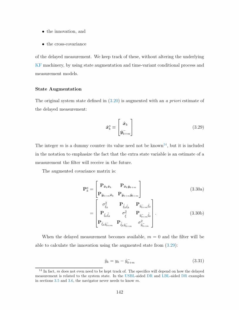
• the innovation, and
• the cross-covariance
of the delayed measurement. We keep track of these, without altering the underlying
KF machinery, by using state augmentation and time-variant conditional process and
measurement models.
State Augmentation
The original system state defined in (3.20) is augmented with an a priori estimate of
the delayed measurement:
xak ≡
xk
y−k+m
(3.29)
The integer m is a dummy counter–its value need not be known14, but it is included
in the notation to emphasize the fact that the extra state variable is an estimate of a
measurement the filter will receive in the future.
The augmented covariance matrix is:
Pak =
PxkxkPxkyk+m
Pyk+mxkPyk+myk+m
(3.30a)
=
σ2ξk
P ˜ξk ξk
Py−k+m
ξk
Pξk
˜ξkσ2˜ξ
Py−k+m
˜ξk
Pξky−
k+mP ˜
ξky−
k+m
σ2y−k+m
. (3.30b)
When the delayed measurement becomes available, m = 0 and the filter will be
able to calculate the innovation using the augmented state from (3.29):
yk = yk − y−k+m (3.31)
14 In fact, m does not even need to be kept track of. The specifics will depend on how the delayedmeasurement is related to the system state. In the USBL-aided DR and LBL-aided DR examplesin sections 3.5 and 3.6, the navigator never needs to know m.
142

and the Kalman gain using the appropriate cross-covariance from (3.30b):
Kk =(
P−xkyk+m
)(
P−yk+myk+m
)−1
(3.32)
Time-Variant Conditional Process Models
Since the original state has been augmented, the process model must be modified to
take this into account. A trigger process model also needs to be defined to allow the
filter to update the augmented state.
The standard augmented process model leaves the a priori estimate of the delayed
measurement unchanged:
xa−k+1 = As
kxa+k (3.33a)
=
1 ∆t 0
−ω2n∆t 1− 2ζωn∆t 0
0 0 1
xa+k (3.33b)
The trigger process model replaces the old measurement estimate with a new one
based on the current state:
xa−k+1 = Atxa+
k (3.34a)
=
1 ∆t 0
−ω2n∆t 1− 2ζωn∆t 0
1 0 0
xa+k (3.34b)
with the same process noise covariance matrix for every step:
Qak =
σ2v1
0 0
0 σ2v2
0
0 0 0
(3.35)
143

Time-Variant Conditional Measurement Models
The velocity sensor runs faster than the delayed position sensor–its measurement
model is:
y−k = Cfastxa−
k (3.36a)
=[
0 1 0]
ξ−kˆξ−k
y−k+m
(3.36b)
when a delayed measurement is available, an alternate measurement model selects its
a priori estimate from the augmented state:
y−k = Cslowxa−
k (3.37a)
=
0 0 1
0 1 0
ξ−kˆξ−k
y−k+m
(3.37b)
switching Ck between Cfast and Cslow based on the conditions of the available mea-
surements ensures that:
• the appropriate innovation is calculated, and
• the correct portions of the augmented covariance matrix are used in calculating
the Kalman gain.
Simulation
Figure 3-5 shows the filter performance for the exact same inputs as Figure 3-3 and
Figure 3-4. This time, the position measurements are still delayed by 0.4 seconds,
but we use the model-driven approach proposed in section 3.3 to compensate for the
delay.
The triggers for switching between conditional process or measurement matrices
are problem-specific. In this example, we have assumed that the filter has knowledge
144

Figure 3-5: Delayed measurements are properly treated using state augmentation andconditional system models.
of which timesteps it will eventually have delayed measurements for. In practice this
is often known, or can at least be estimated. In this example, we used Atrigger once
every Tx1= 0.42 seconds.
Note that in Figure 3-5 the filter performance is comparable to the case with
no delay. By fusing the delayed measurements in a principled and mathematically
rigorous way, we approach the performance of a filter fusing undelayed measurements.
3.4.7 Some comments on alternate approaches
This section presents alternative approaches to delayed measurement fusion. These
ad hoc approaches appear to be simpler and more straightforward, especially when
applied to the simple example system. However, they miss some key advantages of
the more general and flexible method presented in section 3.3.
Given a system with frequent velocity measurements with no delay, and infrequent
position measurements that arrive after an unknown delay, one might consider simply
running the filter in the past and integrating forward in time whenever an estimate of
the current state is needed. If the delayed position measurement relates to timestep
k− l, an external process would calculate the a priori estimate of the current position
145

as:
ξ(t) = ξ(tk−l) +
tk∫
tk−l
ξ(τ)dτ (3.38)
or in discrete time:
ξ−k+1 = ξ−k−l +
k∑
j=k−l
ˆξ+j ∆t (3.39)
The external process would have to recompute the sum at each timestep in the interim
(between when the measurement is valid and when it is available), but that means
storing the velocity at all timesteps in the interval, and recomputing the sum is
unneccessary duplicated effort.
Another approach might be to keep a running average of the velocity, so that
updating the second term on the right hand side of (3.39) could be done faster.
This also requires keeping track of the number of timesteps since the last position
measurement. This method only requires two extra pieces of data. If this running
average and timestep counter were kept within the filter, the process and measurement
equations would become nonlinear and unnecessarily complicated. Otherwise, an
external process would still be required to deal with the running average.
The model-based approach to delayed measurement fusion takes care of all this
automagically. The filter itself tracks position ξ and velocity ξ, effectively increment-
ing through (3.39) at each timestep. By keeping the a priori estimate y−k+m as an
additional state–only keeping one additional piece of information for each delayed
measurement–the filter is able to compute the correct innovation and gain to fuse
the information when the delayed measurement arrives. The key here is that the
KF never really adjusts a posteriori estimates based on measurements–it works using
innovations.
146

3.5 USBL-aided Dead Reckoning
in Two Dimensions
In this example, we study a submerged vehicle navigating by DR with position aiding
from a surface tender using a USBL acoustic tracking system and an acoustic modem.
To keep this example as simple as possible–and focus on the delayed measurement
component of the problem–we will only consider the two-dimensional navigation prob-
lem. We make the following assumptions about measurements:
1. accurate depth (so that we may remove it from the problem),
2. accurate attitude (so that roll and pitch are compensated and we can operate
in the local level frame),
3. the topside portion of the USBL measurement is treated as a black box (dis-
cussed in more detail in the next section).
3.5.1 Mission Scenario
The USBL system uses two-way travel time to estimate the range to a beacon, and the
phase difference between signals at multiple receivers to estimate azimuth and bearing
angles. This relative position measurement is combined with the GPS position of the
tender. The tender transmits the resulting geodetic position fix to the submerged
vehicle via acoustic modem. This is a real-world example of a delayed state problem
and a good example for model-driven delayed measurement fusion.
This mission scenario is becoming more commonplace in both oceanographic and
commercial sectors. The advantage of USBL is that it does not require ship time to
deploy and survey transponder beacons, so it is extremely portable form one site to
another. However, it does require careful calibration of sensor offsets and alignment
between the transducer head, GPS, and an attitude reference. It also requires that
the ship remains in the same area as the vehicle to maintain good tracking during a
mission. This is a non-issue for most tethered and manned vehicles, but other options
such as LBL may be more appropriate for certain types of AUV deployment.
147

GPS
interrogate
GPS
reply
GPS
downlink
Figure 3-6: Typical measurement and communication cycle for USBL-aided DR.First (a), the surface tender interrogates the USBL beacon on the submerged vehicle.The beacon replies (b), and the USBL system reports range, bearing, and azimuthfrom the transducer head to the beacon. This information is fused with the GPSposition and gyrocompass attitude of the tender to compute the geodetic position ofthe beacon. Finally (c), the position fix is transmitted to the vehicle via an acousticmodem. This cycle has a total measurement delay on the order of seconds to tens ofseconds, depending on the distance between the tender and the submerged vehicle.In general, both the vehicle and the ship are moving throughout this measurementcycle.
The observation cycle in this scenario is a simple direct-path acoustic measure-
ment. First, the surface tender interrogates a transponder on the submerged vehicle.
This signal travels through the water column at the depth-averaged sound speed, c,
arriving at the vehicle after a one way travel time delay, τinterrogate. The transpon-
der on the vehicle then waits for a predefined turn-around-time, τtat, before replying.
The reply arrives back at the ship transceiver after another one way travel time delay,
τreply. Processing the solution for the position fix incurs another (hopefully negligi-
ble) delay of length τprocessing. Finally, the ship sends the computed fix to the vehicle,
and it arrives after a third one way travel time delay, τdownlink. This cycle may be
interrupted for many varied reasons (e.g. downlink a command rather than a fix,
lost packets, environmental or ship noise), so the vehicle should not rely on position
updates for safe operation.
148

USBL-aided DR actually has two delayed measurement processes. The topside
process occurs on the ship, and estimates the geographic position of the transpon-
der. The delays associated with this are τinterrogate, τtat, and τreply. As mentioned
earlier, the topside process is treated as a black box in this example–this would be
an interesting research thread to investigate in the future. The vehicle receives a
fully computed geographic fix. Its measurement process is only concerned with the
delays: τreply, τprocessing, and τdownlink. One convenient result of this decoupling is that
the measurement delay in the process on the vehicle can be completely removed in
postprocessing. We will make use of this when comparing the performance of filters
with and without delay compensation.
First-order, two-dimensional kinematic process model
We want to estimate the position of a submerged vehicle by dead reckoning with
position aiding from delayed USBL fixes. We will use a first-order kinematic process
model, with velocity and orientation as inputs. Since depth and attitude are reli-
ably estimated using onboard sensors, we will examine the simplified two-dimensional
problem on a local North-East plane.
The position of the vehicle in the plane evolves with the first-order differential
equation:
x
y
=
cosψ − sinψ
sinψ cosψ
u
v
, (3.40)
where x is positive North, y is positive East, and ψ is the vehicle heading. Veloci-
ties u and v are defined in the vehicle reference frame as forward and starboard, in
accordance with [110].
Define the state vector:
x =
x
y
(3.41)
149

and the input vector:
u =
u
v
ψ
(3.42)
so that the DSSM is:
xk+1 = f (xk,uk, vk) (3.43)
= xk + (Rn
v)k
u1 + v1
u2 + v2
k
∆t (3.44)
where Rn
vis the rotation matrix from the vehicle frame to the navigation frame:
Rn
v=
cos (u3 + v3) − sin (u3 + v3)
sin (u3 + v3) cos (u3 + v3)
(3.45)
and v is process noise.
USBL measurement model
A USBL system could report data as raw two-way travel time and phase information.
In this case, the user would have to integrate platform state to compute a position
fix at each beacon. Most commercial systems will output a relative or absolute fix
in geodetic coordinates. This relieves the user of some responsibility, but now the
system must be treated as a black box.
In this section, we use USBL as an example of a decoupled15 measurement. The
USBL sends fully-resolved position fixes to the vehicle, so it has a direct, but delayed,
measurement model:
yUSBLk = hUSBL (xk−l,wk) (3.46)
15This is called decoupled because each element of the measurement vector corresponds to exactlyone element of the state vector.
150

=[
xk−l +w1,k yk−l +w2,k
]T
(3.47)
· · · xk−l xk−l+1 · · · xk−1 xk xk+1
· · · yk−l yk−l+1 · · · yk−1 yk yk+1
· · · xak−l xa
k−l+1 · · · xak−1 xa
k xak+1
trigger
fuse
downlink
Figure 3-7: Graph of USBL-aided DR. The USBL measurement is a simple obser-vation of the system state at an instant in the past. It draws a diagonal connection(red) from a past state to the current measurement. The trigger conditional processmodel and fuse conditional measurement model manage the augmented states thatserve as extra memory, allowing the system to store information about the systemstate at the instant k − l, when the USBL transponder on the vehicle replied to aninterrogation from the surface ship.
3.5.2 Delay Compensation
Augmented state
Applying the model-driven approach to delayed measurement fusion, we augment the
state vector with an a priori estimate of the delayed measurement:
xa−k =
x−k
y−k+m
=
x−k
y−k
x−k+m
y−k+m
(3.48)
Conditional process models
The augmented standard process model is now:
xa−k+1 = f a
(
xa+k ,uk
)
(3.49a)
151

=
f(
x+k ,uk
)
y−k+m
(3.49b)
= xa+k +
Rnv (u3 + v3)k
u1 + v1
u2 + v2
k
0
0
∆t (3.49c)
and the trigger process model (to update the augmented states) is:
xa−k+1 = fu
(
xa+k ,uk
)
(3.50a)
=
f(
x+k ,uk
)
hUSBL(
x+k , vk
)
(3.50b)
=
I2×2 02×2
I2×2 02×2
xa+k +
Rnv (u3 + v3)k
u1 + v1
u2 + v2
k
0
0
∆t (3.50c)
The condition that chooses the correct process model will vary from problem to
problem. In this example, if the submerged vehicle receives a query ping on the USBL
transponder, it knows to expect a measurement in the future yk+m, that relates to the
state now xk. So, a query ping serves as the trigger16 to activate conditional process
model (3.50c) for one timestep.
Conditional Measurement Models
This particular (simplified) problem only has delayed measurement updates, so the
only conditional measurement model is:
yk = hselect (xk,wk) , (3.51a)
16This assumes that the USBL transponder onboard the vehicle can signal the vehicle when it hasbeen interrogated. This may not be true for all USBL systems, but there is no fundamental reasonpreventing it.
152

y−k =
[
02×2 I2×2
]
xak, (3.51b)
= y−k+m. (3.51c)
Recall that the dummy index m is zero when the delay is over and the measurement
is fused.
Now that the augmented state vector is defined, along with appropriate con-
ditional process and measurement models, this delayed-state sigma point Kalman
filter (DS-SPKF) can be applied to filter real data. We will use field data from a
recent deployment of the AUV Sentry in this example.
3.5.3 Sentry059: Galapagos Ridge
Dive 059 was a standard bathymetric mapping survey along a portion of the Galapagos
rift. Figure 3-8 shows a map view of the first survey block, which provides the
navigation dataset for this example. The dive starts in the Northwest corner with a
short lead-in to the first survey block. Tracklines are oriented East-West, progressing
Southward in a classical lawnmower pattern. The block ends with a Northward
crossing line to provide data for later adjustments based on the multibeam data.
The goal here is to characterize the relative performance of two UKFs: one ig-
noring measurement latency, and the other using augmented states and conditional
models to treat the delayed measurements properly. Since this dataset consists of
real DR and USBL field measurements, there is no absolute ground truth to use as a
baseline. Instead, we adopt a three filter approach: one idealized filter serves as the
basis from which to compare the other two. All filters are UKFs operating with the
same process noise and measurement noise (Table 3.3).
The first filter is the baseline, it operates in postprocessing with complete knowl-
edge of the measurement delays. This filter receives measurements at the instant they
are valid, and fuses them immediately. We will call it the zero delay filter because it
is analogous to the zero delay case in the earlier DHO example.
The second filter is a traditional UKF based on (3.44) and (3.47). It receives
153

Figure 3-8: Map view of the first survey block on Sentry dive 059. The tracklinesin this block are oriented East-West, which is convenient for comparing filters withand without delay compensation since delays manifest as alongtrack error. USBLfixes are shown as blue dots. The black, red, and green lines are position estimatesgiven by the UKF with no delay, untreated delay, and treated delay, respectively. Theestimates are indistinguishable at this scale–Figure 3-9 shows the differences betweenthem.
154

Table 3.3: Timing, process noise, and measurement noise parameters used in renavi-gation of dive 059.
T fast T slow l σv1, σv2
σv3σw1
, σw2
s s - m/s rad m
0.2 O(1− 10) 20-30 0.04 0.001 5.0
measurements after the USBL has computed a fix and it has been sent to the vehicle
via acoustic modem17. However, this filter ignores the fact that these measurements
are delayed, so we call its estimates ‘untreated.’
The third filter uses the delayed-state Kalman filter (DS-KF) approach. It receives
identical measurements at the same time as the second filter, but calculates the correct
delayed residual before fusing them with the current state. We call the estimates from
this filter ‘treated.’
We compare the relative performance of filters 2 and 3 by examining the position
residuals of the treated and untreated estimates. These residuals are defined:
runtreated = xzero delay − xuntreated (3.52)
rtreated = xzero delay − xtreated (3.53)
Recall that these are not residuals relative to a ground-truth.
Figure 3-9 shows absolute values for North and East residuals, as well as the
magnitude of the total two-dimensional residual vector. The untreated estimates
are worse alongtrack (i.e. East-West) than across-track (i.e North-South). This is
expected because the delayed measurements correspond to spatial errors opposite the
direction of travel. Note that the treated estimates are much closer to the baseline
by all measures. Furthermore, the residuals of the treated measurements are lower
than the USBL measurement noise standard deviation.
17Automatic acoustic downlink of position fixes was not implemented for dive 059, so this timinghas been estimated based on two-way travel times measured during the dive.
155

Figure 3-9: Absolute values of position residuals from the UKF estimates with un-treated delay (red) and treated delay (green), plotted on a log scale. The baseline isgiven by position estimates of the UKF postprocessed with zero delay. 1σ, 2σ, and3σ confidence intervals of the zero delay filter are shown in black for reference.
156

3.6 LBL-aided Dead Reckoning
in Three Dimensions
This section demonstrates the model-driven approach to delayed measurement fu-
sion on another application in underwater navigation–LBL-aided dead reckoning. We
will briefly review long baseline acoustic navigation, then define the standard kine-
matic process model, then define the LBL measurement model. We then define an
augmented state and adjusted process and measurement models to support asyn-
chronous, delay-compensated aiding from the LBL system. We demonstrate the de-
layed measurement SPKF using navigational data from Sentry dive 073–a preliminary
bathymetric mapping mission within a three-transponder LBL net.
3.6.1 Mission Scenario
Long baseline acoustic positioning (LBL) provides delayed, but drift free, measure-
ments of vehicle position at a low update rate. In precision underwater navigation,
LBL measurements bound the error growth of high-rate DR or INS navigation.
LBL positioning uses ranges from two or more fixed underwater acoustic transpon-
ders to localize another transponder, usually on a submerged vehicle or instrument
package [3]. The globally referenced transponder positions are surveyed by a ship
when the LBL net is deployed. In spherical LBL positioning18, the vehicle interro-
gates the net with an acoustic signal, and each transponder replies in a unique way.
Given an estimate of the sound speed through the water, the measured two-way travel
times produce estimates of the slant range between the vehicle and each transponder
in the net.
LBL works like an acoustic version of GPS underwater–you just have to provide
your own beacons (satellites). The cost is in the ship time spent deploying and
surveying the transponders19–once that is done, the ship is free to leave the area for
18Hyperbolic LBL positioning, on the other hand, uses a passive receiver and synchronized beacons.The receiver position is calculated using the difference in ranges to the two beacons [4, 5]. We willfocus on spherical LBL for the remainder of this section.
19and recovering them afterward
157

other tasks. An AUV can continue to operate unattended without position updates
from the ship and without its navigation error growing unbounded. This flexibility
makes LBL a good solution when operations will be in the same area for several days.
However, the travel times and subsequent slant ranges used in LBL positioning are
inherently delayed. This motivates an explicit and rigorous treatment of the delay,
and makes LBL-aided DR an interesting example application for the model-driven
approach to delayed measurement fusion presented in section 3.3.
Second-order, three dimensional kinematic process model
Using the standard notation for a submerged body [110, 111], the state is:
x =[
ηT1 νT
1 ηT2
]T
(3.54a)
=[
x y z u v w φ θ ψ]T
(3.54b)
The positions x, y, z are positive North, East, and Down in the local navigation
frame. The velocities u, v, w are positive forward, starboard, and toward the keel in
the moving vehicle frame. And, the Euler angles20 φ, θ, ψ describe roll, pitch, and
heading.
The process model is:
x−k+1 = f
(
x+k ,uk, vk
)
(3.55)
= x+k +
(Rn
v)k (x3:6)
+k
uk + vk
∆t (3.56)
where (Rn
v)k ∈ SO(3) is the rotation matrix from the vehicle frame to the navigation
frame, calculated from the Euler angles.
20Alternate attitude representations are better, but Euler angles are used in this example because1) this is standard, so it will be most accessible 2) the fiber-optic gyroscope (FOG) on Sentry ouputsEuler angles in its standard configuration 3) the FOG measurement is precise enough that it iseffectively driving the attitude variables as a control input.
158

DVL measurement model
The measurement equation for DVL bottom-track velocities in instrument coordinates
is:
yDVLk = hDVL, i (xk,wk) (3.57a)
= Riv
uk
vk
wk
+wk (3.57b)
y−k = Ri
v
u−k
v−k
w−k
(3.57c)
where Riv is the rotation matrix describing the misalignment between vehicle and
DVL instrument reference frames.
FOG measurement model
The measurement equation for vehicle orientation from the FOG is:
yFOGk = hFOG (xk,wk) (3.58a)
=
φk
θk
ψk
+wk (3.58b)
y−k =
φ−k
θ−k
ψ−k
(3.58c)
Standard LBL measurement model
Traditional LBL without delay compensation Figure 3-10 assumes that the vehicle
and beacon are stationary over the interrogation period and that returns from all
159

interrogate
reply
interrog
ate
reply
Figure 3-10: LBL acoustic positioning using two-way travel times from multiple un-derwater transponders. The vehicle interrogates the net, and each transponder replieson its own unique frequency. The two-way travel times give estimated ranges to eachtransponder. Combined with the known positions of the transponders, the rangesprovide an observation of the vehicle position.
beacons are available at the same time. The position of the vehicle is then calculated
by trilateration. If more ranges are available, the problem is solved using nonlinear
least squares (LS) [112]:
xk = argminxk
n∑
i=0
∥
∥
∥
∥
(
c
τtwtt
)
i
− ‖xbi − xk‖∥
∥
∥
∥
(3.59)
We could use LBL measurements like this in the same loosely-coupled fashion that we
used USBL measurements in section 3.5. However, the complex nature of the delay
in LBL measurements suggests a different way.
Asynchronous LBL measurement model
Here we use LBL-aiding as an example of a more tightly integrated measurement.
We update the position estimate of the vehicle asynchronously, fusing travel time
innovations as the response from each beacon in the net is received. One advantage
of this approach is that the navigator can perform a partial position update even if
160
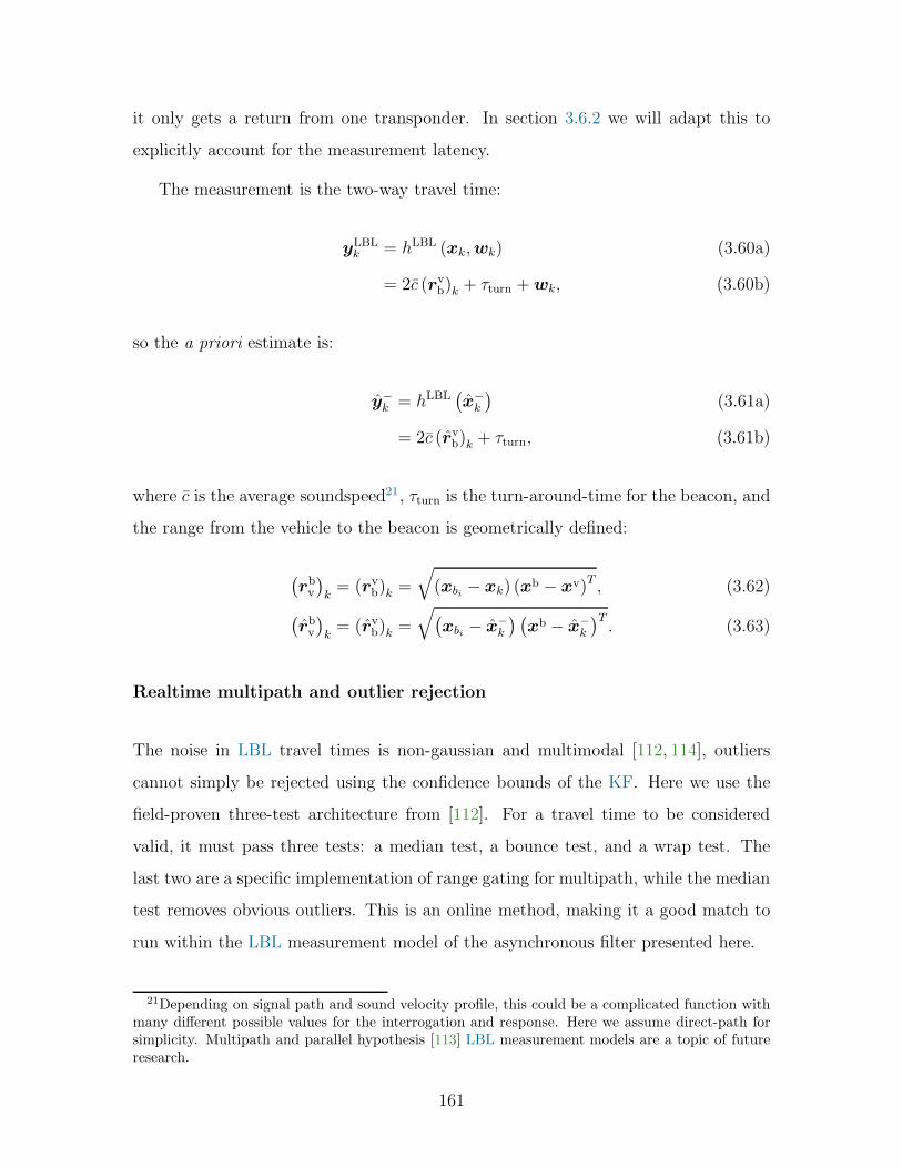
it only gets a return from one transponder. In section 3.6.2 we will adapt this to
explicitly account for the measurement latency.
The measurement is the two-way travel time:
yLBLk = hLBL (xk,wk) (3.60a)
= 2c (rvb)k + τturn +wk, (3.60b)
so the a priori estimate is:
y−k = hLBL
(
x−k
)
(3.61a)
= 2c (rvb)k + τturn, (3.61b)
where c is the average soundspeed21, τturn is the turn-around-time for the beacon, and
the range from the vehicle to the beacon is geometrically defined:
(
rbv
)
k= (rv
b)k =
√
(xbi − xk) (xb − xv)T , (3.62)
(
rbv
)
k= (rv
b)k =
√
(
xbi − x−k
) (
xb − x−k
)T. (3.63)
Realtime multipath and outlier rejection
The noise in LBL travel times is non-gaussian and multimodal [112, 114], outliers
cannot simply be rejected using the confidence bounds of the KF. Here we use the
field-proven three-test architecture from [112]. For a travel time to be considered
valid, it must pass three tests: a median test, a bounce test, and a wrap test. The
last two are a specific implementation of range gating for multipath, while the median
test removes obvious outliers. This is an online method, making it a good match to
run within the LBL measurement model of the asynchronous filter presented here.
21Depending on signal path and sound velocity profile, this could be a complicated function withmany different possible values for the interrogation and response. Here we assume direct-path forsimplicity. Multipath and parallel hypothesis [113] LBL measurement models are a topic of futureresearch.
161

3.6.2 Delay Compensation
Careful thought about the nature of a two-way travel time LBL measurement leads
to the realization that a two-way travel time is really the sum of two one-way travel
times. This may seem obvious, but consider: it is actually the sum of two different
one-way travel times22 (see Figure 3-11):
interrogation the travel time from the vehicle to the beacon, and
reply the travel time from the beacon back to the vehicle.
Assuming the beacon is stationary (as we have been all along), each of these travel
times can be estimated independently by the vehicle in realtime. The interrogation
travel time is based on the range from the vehicle to the beacon at the instant the
vehicle pings the net:
yowttk−l = τ biinterrogate = howtt (xk−l,xbi, c(z)) , (3.64a)
=1
c‖rbi
k−l‖2, (3.64b)
=1
c
√
(xk − xbi)(xk − xbi)T . (3.64c)
The reply travel time is based on the range from the beacon to the vehicle at the
instant the vehicle receives the return:
yowttk = τ bireply = howtt (xk,xbi, c(z)) , (3.65a)
=1
c‖rbi
k ‖2, (3.65b)
=1
c
√
(xk − xbi)(xk − xbi)T . (3.65c)
22This is not a novel observation, but many existing implementations ignore this fact. Explicitdelay compensation is necessary to handle an LBL measurement this way. After formulating theproblem independently using the model-driven approach presented in this research, it was broughtto my attention that a similar treatment existed in [104]. That work uses state augmentation witha full state copy to handle delayed measurements, as discussed in section 3.1.2.
162

interrogate
interrogate
interrogate
reply
interrogate
reply
Figure
3-11:Measurementcycleforasynchronou
s,delay-com
pensatedLBL-aided
DR
withon
ebeacon.First,thesubmerged
vehicle
interrogates
theLBL
tran
spon
der.After
aknow
nturn-aroundtime,
thetran
spon
der
replies
onauniquefrequency.
When
thevehicle
receives
thereply,it
computestheinnovationfrom
themeasuredthetw
o-way
travel
timean
dad
justsits
positionestimateaccordingly.
Thiscyclehas
atotalmeasurementdelay
ontheorder
ofsecondsto
tensof
seconds,
dep
ending
onthedistance
betweenthevehicle
andthetran
spon
der.In
general,thevehicle
ismovingduringthedelay,so
itspositionat
theinstan
titinterrogates
thetran
spon
der
isdifferentthan
itspositionwhen
itreceives
thereply.Thepositionisalso
different
when
itreceives
areply
from
adifferenttran
spon
der.Asthevehicle
receives
replies
from
each
tran
spon
der,thenavigation
uncertainty
inthepositionestimateshrinksalon
gthelinebetweenthevehicle
andthat
particulartran
spon
der.
163
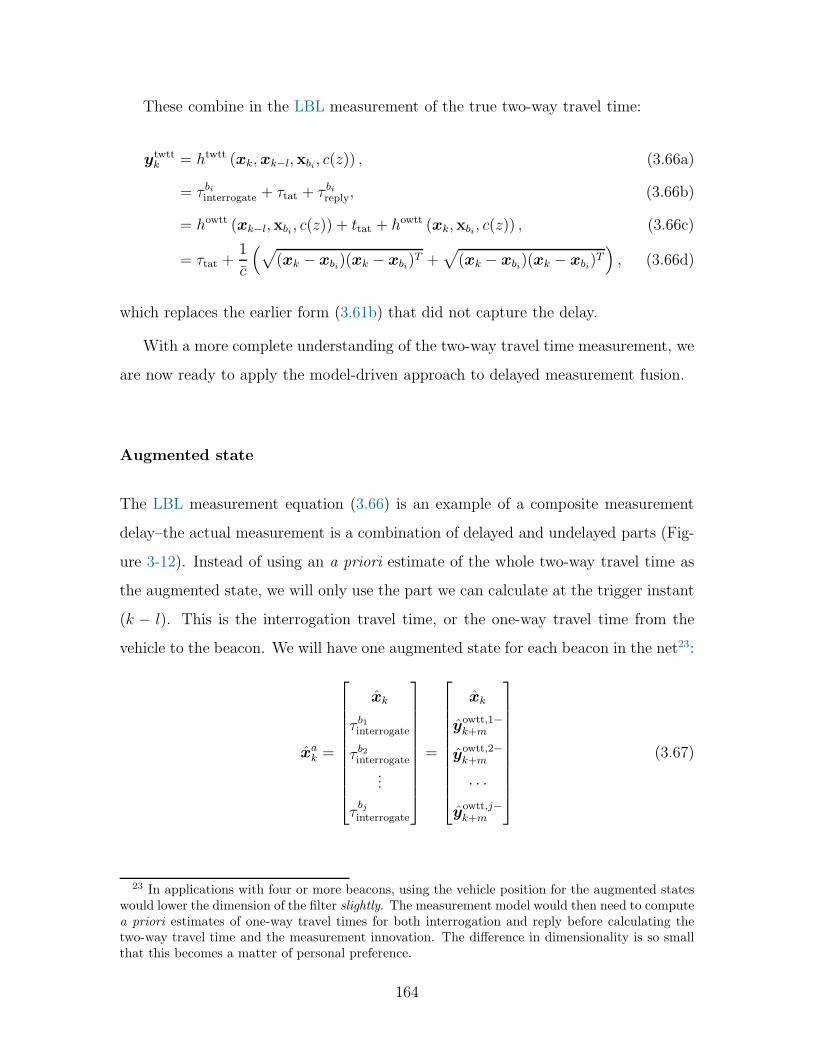
These combine in the LBL measurement of the true two-way travel time:
ytwttk = htwtt (xk,xk−l,xbi , c(z)) , (3.66a)
= τ biinterrogate + τtat + τ bireply, (3.66b)
= howtt (xk−l,xbi , c(z)) + ttat + howtt (xk,xbi , c(z)) , (3.66c)
= τtat +1
c
(
√
(xk − xbi)(xk − xbi)T +
√
(xk − xbi)(xk − xbi)T)
, (3.66d)
which replaces the earlier form (3.61b) that did not capture the delay.
With a more complete understanding of the two-way travel time measurement, we
are now ready to apply the model-driven approach to delayed measurement fusion.
Augmented state
The LBL measurement equation (3.66) is an example of a composite measurement
delay–the actual measurement is a combination of delayed and undelayed parts (Fig-
ure 3-12). Instead of using an a priori estimate of the whole two-way travel time as
the augmented state, we will only use the part we can calculate at the trigger instant
(k − l). This is the interrogation travel time, or the one-way travel time from the
vehicle to the beacon. We will have one augmented state for each beacon in the net23:
xak =
xk
τ b1interrogate
τ b2interrogate...
τbjinterrogate
=
xk
yowtt,1−k+m
yowtt,2−k+m
· · ·yowtt,j−k+m
(3.67)
23 In applications with four or more beacons, using the vehicle position for the augmented stateswould lower the dimension of the filter slightly. The measurement model would then need to computea priori estimates of one-way travel times for both interrogation and reply before calculating thetwo-way travel time and the measurement innovation. The difference in dimensionality is so smallthat this becomes a matter of personal preference.
164
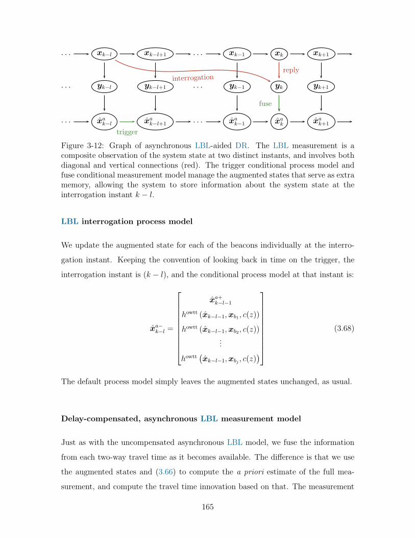
· · · xk−l xk−l+1 · · · xk−1 xk xk+1
· · · yk−l yk−l+1 · · · yk−1 yk yk+1
· · · xak−l xa
k−l+1 · · · xak−1 xa
k xak+1
trigger
fuse
interrogationreply
Figure 3-12: Graph of asynchronous LBL-aided DR. The LBL measurement is acomposite observation of the system state at two distinct instants, and involves bothdiagonal and vertical connections (red). The trigger conditional process model andfuse conditional measurement model manage the augmented states that serve as extramemory, allowing the system to store information about the system state at theinterrogation instant k − l.
LBL interrogation process model
We update the augmented state for each of the beacons individually at the interro-
gation instant. Keeping the convention of looking back in time on the trigger, the
interrogation instant is (k − l), and the conditional process model at that instant is:
xa−k−l =
xa+k−l−1
howtt (xk−l−1,xb1, c(z))
howtt (xk−l−1,xb2, c(z))...
howtt(
xk−l−1,xbj , c(z))
(3.68)
The default process model simply leaves the augmented states unchanged, as usual.
Delay-compensated, asynchronous LBL measurement model
Just as with the uncompensated asynchronous LBL model, we fuse the information
from each two-way travel time as it becomes available. The difference is that we use
the augmented states and (3.66) to compute the a priori estimate of the full mea-
surement, and compute the travel time innovation based on that. The measurement
165

equation is:
y−k = ha−twtt (xa
k,xbi, c(z)) (3.69a)
= τ biinterrogate + τtat + τ bireply, (3.69b)
= hselect (xak, bi) + τtat + howtt (xa
k,xbi, c(z)) , (3.69c)
where hselect (xak, bi) simply selects the interrogation one-way travel time for the rele-
vant transponder from the augmented states.
The filter continues to run until it receives a reply from another beacon, at which
time it fuses that measurement. The augmented states are not updated until the
interrogation at the beginning of the next LBL cycle.
3.6.3 Sentry073: Hakon Mosby Mud Volcano
This section evaluates the performance of the asynchronous LBL-aided DR filter using
navigational data from field deployments of the oceanographic AUV Sentry. We will
compare the estimates from the fully delay compensated filter to two different filters:
interrogate assumes the two-way travel time is an observation of the system state
only at the time the vehicle interrogates the net24, and
reply assumes the two-way travel time is an observation of the system state only at
the time the vehicle receives the reply.
Unfortunately, due to the complex nature of LBL measurement delay, it is not possible
to implement a comparable filter with the delays artificially removed25 as we did in
section 3.5.3.
The LBL-aided DR filter was used to renavigate data from Sentry073, the initial
multibeam survey during a research cruise in September/October 2010 on the Hakon
24Note that this filter still requires delay treatment, because the two-way travel time measurementis not available at the interrogation instant.
25One might consider doing this in a more traditional LBL system with explicit calculation ofgeographic position fixes, but that is not directly comparable to the asynchronous approach takenhere.
166

0 500 1000 1500 2000 2500 3000
eastings [m]
0
500
1000
1500
2000
2500
northings[m
]
PPL
compensated
start
end
Figure 3-13: Map view of the initial multibeam survey mission Sentry dive 073.The tracklines in this block are oriented North-South. The locations of the threetransponders in the 12 kHz LBL net are marked by colored circles. The black linemarked PPL uses the DSL standard postprocessing with traditional LBL and explicitposition fixes. The green line is the fully delay compensated realtime LBL-aided DRfilter detailed in this section. The fundamental difference in LBL measurement fusionmakes a direct comparison of these two trajectories questionable, but the PPL trackis useful as a sanity check for the realtime filter.
Mosby mud volcano in the Barents Sea. These dives were part of a research cruise
led by Dr. Antje Boetius with the goal of characterizing the bathymetry, sub-bottom
composition, and chemistry surrounding the mud volcano.
Figure 3-13 shows the trajectory of Sentry during this first dive, and the locations
of the three transponders in the LBL net that the Sentry team deployed and surveyed
prior to the dive. After two crossing lines at the beginning of the dive, the tracklines
are primarily North-South, covering over 68 kilometers at an average speed of 1 m/s
and and average depth of 1245 m. Figure 3-14 shows the components of the vehicle
position throughout the dive.
167

18:00:00
20:00:00
22:00:00
00:00:00
02:00:00
04:00:00
06:00:00
08:00:00
10:00:00
12:00:00
14:00:00
0
500
1000
1500
2000
2500
North
18:00:00
20:00:00
22:00:00
00:00:00
02:00:00
04:00:00
06:00:00
08:00:00
10:00:00
12:00:00
14:00:00
0
500
1000
1500
2000
2500
East
18:00:00
20:00:00
22:00:00
00:00:00
02:00:00
04:00:00
06:00:00
08:00:00
10:00:00
12:00:00
14:00:00
time(U
TC)
0
200
400
600
800
1000
1200
1400
Down
PPL
interro
gate
reply
compensated
positio
ns[m
]
Figu
re3-14:
Com
pon
ents
ofveh
icleposition
durin
gSentry
073.
168

−10
−505
10
North
18:00:00
20:00:00
22:00:00
00:00:00
02:00:00
04:00:00
06:00:00
08:00:00
10:00:00
12:00:00
14:00:00
−10
−505
10
East
interrogate
reply
compensated-uncompensated
Figure
3-15:Horizon
talpositiondifferencesbetweenasynchronou
sLBL-aided
DR
filterson
Sentry073.
Thereis
nogrou
nd
truth
(thisisfielddata)
andnocomparab
lezero-delay
reference
filter
(dueto
thecompositenature
oftheLBLdelay).
So,
we
use
thefullycompensatedfilter
asthereference
andcomparetheestimates
producedbytheother
twofilters.
Thedifferences
arevariab
le,on
theorder
ofmeters,an
dforthemostpartlarger
than
theconfidence
bou
ndsshow
nin
Figure
3-16.
169

Figure 3-14 shows the horizontal26 components of the difference between vehicle
position estimated by the fully delay compensated filter and the filters assuming τ twtt
is based solely on the interrogation state and assuming τ twtt is based solely on the reply
state, respectively. The position estimates of the different filters vary on the order of
1-10 m, with a periodicity that may be linked to the change in directions progressing
through tracklines. Unfortunately, without an independent ground truth, it is difficult
to say with certainty which estimate is most correct–the measurement equation (3.66)
for the fully delay compensated filter certainly reflects the true nature of the two-way
travel time most closely. Figure 3-16 shows the filter confidence intervals in North
and east directions throughout the course of the dive. Despite having the same filter
parameters and receiving the exact same measurements from all navigational sensors,
the filters with LBL measurement models based solely on interrogation state and
reply state have larger confidence intervals than the fully delay compensated filter.
This indicates that the models in the fully delay compensated filter may be more
consistent with the measurements it is receiving.
3.7 Discussion and Conclusions
We’ve presented a flexible, model-driven approach to fuse information from delayed
measurements in realtime. We used the proven framework of Kalman filter, and our
model-driven approach does not change any of the underlying machinery of the KF.
The delay treatment is mathematically rigorous and optimal for linear systems–it is a
tractable, efficient, and principled approach for nonlinear systems. We characterized
the estimation error using a simulation of a simple canonical system, then applied the
approach to the real-world problem of navigating an underwater vehicle in the deep
ocean, both with a decoupled example (USBL-aided DR) and with a more integrated
example (LBL-aided DR).
This is really just the beginning. With a straightforward approach to delayed
26We don’t show the vertical component simply because undelayed measurement from the pressuredepth sensor constrain this state similarly for all three filters.
170

10−1
100
101
σNorth[m]
18:00:00
20:00:00
22:00:00
00:00:00
02:00:00
04:00:00
06:00:00
08:00:00
10:00:00
12:00:00
14:00:00
10−1
100
101
σEast[m]
compensated
interrogate
reply
Figure
3-16:Horizon
talpositionconfidence
intervalsof
asynchronou
sLBL-aided
DRfilterson
Sentry073.
Thefullycompensated
filter
has
its1σ
confidence
bou
ndat
abou
t30
cmacrosstrack(E
ast-West)
and30-40cm
alon
gtrack
(North-Sou
th).
171

measurement fusion based on the workhorse KF framework, future directions to in-
vestigate might include:
• principled delay treatment in internal estimates of the shipboard USBL system
• other operations concepts and associated delay structures (e.g., USBL on a
tethered vehicle like an ROV)
• more complicated acoustic travel time models using raytracing
• incorporating measurements from bounce (return) paths of LBL without needing
any additional augmented states.
• incorporating wrapped LBL replies in very long range missions by using addi-
tional augmented states
• using the asynchronous LBL example presented here, with explicit delay com-
pensation, in a single transponder or mobile transponder navigation scenario
172

Chapter 4
Discussion and Conclusions
This dissertation has presented details on three contributions to the art of automated
realtime underwater navigation. The theory behind each of these contributions has
been explained in detail. And each contribution has been demonstrated in simula-
tion, with laboratory data, or in the field. Some of these contributions have been
demonstrated in all three arenas.
Here we briefly review the results and conclusions from each chapter, and comment
on promising future directions for each research thread.
Navigation Sensor Alignment
We presented the Doppler velocity log (DVL)/fiber-optic gyroscope (FOG) sensor
alignment problem and posed it as a general rotation identification problem. After
expressing the problem in Geometric Algebra (GA), we proposed a simple adaptive
identifier and proved its asymptotic stability. We demonstrated this identifier in
simulation, then applied it to DVL/FOG alignment on underwater vehicles in the
laboratory and in the field. Using the alignment estimated by the rotor identifier in
dead reckoning (DR) improved agreement of the position estimate with long baseline
(LBL) observations. The rotor identifier performed comparably to previously reported
techniques based on rotation matrices.
Future directions one might take with the rotor identifier include:
173

• investigation of the acceleration-velocity form of DVL/inertial navigation system
(INS) alignment as studied using rotation matrices in [62, 63]
• a proportional-derivative form of the identifier for enhanced noise rejection and
increased control of identifier dynamics
• an identifier on the full group of rigid-body motions–rotation as well as translation–
using rotors in a higher dimensional GA
• applications to align other sensors (camera, multibeam, etc. . . )
Finally, the clarity and intuition gained by posing the rotation identification problem
in GA has proven useful in this first application of GA to underwater robotics. It is
possible that similar benefits are waiting if we apply GA to other underwater problems
(e.g., hydrodynamics, the full six degree-of-freedom navigation equations, or control
problems)
Dead reckoning through the water column
We proposed a method for dead reckoning through the water column using overlapping
water profile measurements collected by a vehicle-mounted acoustic Doppler current
profiler (ADCP). We demonstrated this proof of concept using three implementations:
• an online bin average approach,
• a batch weighted least squares (WLS) approach, and
• an online recursive least squares (RLS) approach.
We applied these implementations to data from the ascent at the end of several
Sentry missions, and compared the DR track to external ultra-short baseline (USBL)
observations where possible.
Although this technique is not quite ready for field service on deep autonomous
underwater vehicles (AUVs), it holds great promise. Dead reckoning using ADCP
water profile measurements enhances the autonomy of underwater vehicles because it
174

enables underwater navigation without dependence on external systems. It provides
a link between Global Positioning System (GPS) at the surface and DR or terrain-
relative navigation near the seafloor.
Future work in this thread should focus on demonstrating a full operation–from
surface to seafloor and back–on a small AUV, possibly with higher frequency ADCP.
Model-driven delayed measurement fusion
We’ve presented a flexible, model-driven approach to fuse information from delayed
measurements in realtime. We used the proven framework of Kalman filter, and
our model-driven approach does not change any of the underlying machinery of the
Kalman filter (KF). We demonstrated the approach in simulation on a damped har-
monic oscillator (DHO), and showed that the filter with explicit delay compensation
approached the performance of a filter without any measurement delay. We replicated
this result using real-world data from Sentry for USBL-aided DR, then applied it to
asynchronous LBL-aided DR, again using field data from Sentry.
With a straightforward approach to delayed measurement fusion based on the
workhorse KF framework, future directions to investigate might include:
• rigorous delay treatment in internal estimates of the shipboard USBL system
• other operations concepts and associated delay structures (e.g., USBL on a
tethered vehicle like an remotely operated vehicle (ROV))
• more complicated acoustic travel time models using raytracing
• incorporating measurements from bounce (return) paths of LBL without needing
any additional augmented states.
• incorporating wrapped LBL replies in very long range missions by using addi-
tional augmented states
• using the asynchronous LBL example presented here, with explicit delay com-
pensation, in a single transponder or mobile transponder navigation scenario
175

The sigma point Kalman filter (SPKF) foundation of the USBL-aided DR and LBL-
aided DR field examples is ideally posed to leverage high-fidelity dynamic vehicle
models. Including these (instead of a simple kinematic model) will make each filter
implementation vehicle- or application specific, but promises the added benefit of
robustness to sensor outages and potentially increased capability for fault detection.
In the end, I find the more I know, the less I know. This dissertation has raised
more questions than it has answered, but it has answered the ones it set out to.
Underwater navigation remains an interesting and challenging field, one simply has
to choose the next topic and dive in.
176

Bibliography
[1] J. Buffett, Where is Joe Merchant? : A Novel Tale. Harcourt Brace Jovanovich,August 1992.
[2] N. P. Fofonoff and R. C. Millard Jr., “Algorithms for computation of fundamen-tal properties of seawater,” in UNESCO Technical Papers in Marine Science.Place de Fontenoy, 75700 Paris, France: UNESCO Division of Marine Sciences,1983, no. 44.
[3] M. M. Hunt, W. M. Marquet, D. A. Moller, K. R. Peal, W. K. Smith, and R. C.Spindel, “An acoustic navigation system,” Woods Hole Oceanographic Institu-tion, Woods Hole, MA, Technical Report 74-6, December 1974, unpublishedmanuscript.
[4] P. H. Milne, Underwater Acoustic Positioning Systems. Gulf Publishing Com-pany, 1983.
[5] M. V. Jakuba, C. N. Roman, H. Singh, C. Murphy, C. Kunz, C. Willis, T. Sato,and R. A. Sohn, “Long-baseline acoustic navigation for under-ice autonomousunderwater vehicle operations,” Journal of Field Robotics, vol. 25, no. 11-12,pp. 861 – 879, 2008. [Online]. Available: http://dx.doi.org/10.1002/rob.20250
[6] L. L. Whitcomb, D. R. Yoerger, H. Singh, and J. C. Howland, “Advances inunderwater robot vehicles for deep ocean exploration: Navigation, control, andsurvey operations,” in Proceedings of the International Symposium of RoboticsResearch (ISRR), Snowbird, UT, October 1999.
[7] J. C. Kinsey, R. M. Eustice, and L. L. Whitcomb, “A survey of underwatervehicle navigation: Recent advances and new challenges,” in IFAC Conferenceof Manoeuvering and Control of Marine Craft, Lisbon, Portugal, September2006, invited paper.
[8] M. Larsen, “Synthetic long baseline navigation of underwater vehicles,” in Pro-ceedings of OCEANS, vol. 3. MTS/IEEE, 2000, pp. 2043–2050.
[9] C. E. G. LaPointe, “Virtual long baseline (VLBL) autonomous underwatervehicle navigation using a single transponder,” Master’s thesis, MassachusettsInstitute of Technology and Woods Hole Oceanographic Institution, Cambridgeand Woods Hole, MA, June 2006.
177

[10] B. Jalving, K. Gade, O. Hagen, and K. Vestgard, “A toolbox of aiding tech-niques for the HUGIN AUV integrated inertial navigation system,” in Proceed-ings of OCEANS, vol. 2. MTS/IEEE, September 2003, pp. 1146–1153.
[11] O. Hegrenaes, K. Gade, O. Hagen, and P. Hagen, “Underwater transponderpositioning and navigation of autonomous underwater vehicles,” in Proceedingsof OCEANS. MTS/IEEE, October 2009.
[12] J.-P. Peyronnet, R. Person, and F. Rybicki, “POSIDONIA 6000: a new longrange highly accurate ultra short base line positioning system,” in Proceedingsof OCEANS, vol. 3. Nice, France: MTS/IEEE, September 1998, pp. 1721–1727. [Online]. Available: http://dx.doi.org/10.1109/OCEANS.1998.726382
[13] J. C. Kinsey and L. L. Whitcomb, “In situ alignment calibration of attitudeand Doppler sensors for precision underwater vehicle navigation: Theory andexperiment,” IEEE Journal of Oceanic Engineering, vol. 32, no. 2, pp. 286–299,April 2007. [Online]. Available: http://dx.doi.org/10.1109/JOE.2007.893686
[14] ——, “Adaptive identification on the group of rigid-body rotations andits application to underwater vehicle navigation,” IEEE Transactions onRobotics, vol. 23, no. 1, pp. 124–136, February 2007. [Online]. Available:http://dx.doi.org/10.1109/TRO.2006.886829
[15] M. J. Stanway and J. C. Kinsey, “Sensor alignment using rotors in geometricalgebra,” in Proceedings of the International Conference on Robotics andAutomation (ICRA). Shanghai, China: IEEE, May 2011, pp. 994–999.[Online]. Available: http://dx.doi.org/10.1109/ICRA.2011.5980519
[16] W. Alameda Jr, “Seadevil-A totally integrated inertial navigation system (INS)solution,” in Proceedings of the Underwater Intervention Symposium, New Or-leans, LA, 2002.
[17] Navigator Doppler Velocity Log Technical Manual, Teledyne RD Instruments,Poway, CA, November 2006.
[18] N. Brokloff, “Matrix algorithm for Doppler sonar navigation,” in Proceedingsof OCEANS, vol. 3. MTS/IEEE, September 1994, pp. 378–383. [Online].Available: http://dx.doi.org/10.1109/OCEANS.1994.364228
[19] L. Whitcomb, D. Yoerger, and H. Singh, “Advances in doppler-basednavigation of underwater robotic vehicles,” in Proceedings of the InternationalConference on Robotics and Automation (ICRA), vol. 1. IEEE, May 1999, pp.399–406. [Online]. Available: http://dx.doi.org/10.1109/ROBOT.1999.770011
[20] L. Whitcomb, D. Yoerger, H. Singh, and D. Mindell, “Towards precisionrobotic maneuvering, survey, and manipulation in unstructured undersea envi-ronments,” in Proceedings of the International Symposium on Robotics Research(ISRR), vol. 8, 1998, pp. 45–54.
178

[21] J. C. Kinsey and L. L. Whitcomb, “Preliminary field experience with the DVL-NAV integrated navigation system for oceanographic submersibles,” ControlEngineering Practice, vol. 12, no. 12, pp. 1541–1548, December 2004.
[22] P. Miller, J. Farrell, Y. Zhao, and V. Djapic, “Autonomous underwater vehiclenavigation,” IEEE Journal of Oceanic Engineering, vol. 35, no. 3, pp. 663 –678,July 2010. [Online]. Available: http://dx.doi.org/10.1109/JOE.2010.2052691
[23] R. McEwen, H. Thomas, D. Weber, and F. Psota, “Performance of anAUV navigation system at Arctic latitudes,” IEEE Journal of OceanicEngineering, vol. 30, no. 2, pp. 443–454, April 2005. [Online]. Available:http://dx.doi.org/10.1109/JOE.2004.838336
[24] N. Brokloff, “Dead reckoning with an ADCP and current extrapolation,” inProceedings of OCEANS, vol. 2. MTS/IEEE, October 1997, p. 1411. [Online].Available: http://dx.doi.org/10.1109/OCEANS.1997.624203
[25] E. Firing and R. Gordon, “Deep ocean acoustic doppler current pro-filing,” in Proceedings of the IEEE Fourth Working Conference onCurrent Measurement, April 1990, pp. 192 –201. [Online]. Available:http://dx.doi.org/10.1109/CURM.1990.110905
[26] J. Fischer and M. Visbeck, “Deep velocity profiling with self-contained ADCPs,” Journal of Atmospheric and Oceanic Tech-nology, vol. 10, no. 5, pp. 764–773, 1993. [Online]. Available:http://dx.doi.org/10.1175/1520-0426(1993)010%3C0764:DVPWSC%3E2.0.CO;2
[27] M. Visbeck, “Deep velocity profiling using lowered acoustic Doppler currentprofilers: Bottom track and inverse solutions,” Journal of Atmospheric andOceanic Technology, vol. 19, no. 5, pp. 794–807, 2002. [Online]. Available:http://dx.doi.org/10.1175/1520-0426(2002)019%3C0794:DVPULA%3E2.0.CO;2
[28] M. J. Stanway, “Water profile navigation with an acoustic Doppler current pro-filer,” in Proceedings of OCEANS. Sydney, Australia: MTS/IEEE, May 2010.[Online]. Available: http://dx.doi.org/10.1109/OCEANSSYD.2010.5603647
[29] ——, “Dead reckoning through the water column with an acoustic Doppler cur-rent profiler: Field experiences,” in Proceedings of OCEANS. Kona, Hawai’i:IEEE, September 2011.
[30] L. Medagoda, M. Jakuba, O. Pizarro, and S. Williams, “Water column currentprofile aided localisation for autonomous underwater vehicles,” in Proceedingsof OCEANS. Sydney, Australia: IEEE, May 2010.
[31] L. Medagoda, S. B. Williams, O. Pizarro, and M. V. Jakuba, “Water col-umn current profile aided localisation combined with view-based SLAM for au-tonomous underwater vehicle navigation,” in Proceedings of the InternationalConference on Robotics and Automation (ICRA). Shanghai, China: IEEE,May 2011.
179

[32] D. Meduna, S. Rock, and R. McEwen, “Low-cost terrain relative navigationfor long-range AUVs,” in Proceedings of OCEANS. MTS/IEEE, September2008. [Online]. Available: http://dx.doi.org/10.1109/OCEANS.2008.5152043
[33] ——, “Closed-loop terrain relative navigation for AUVs with non-inertial grade navigation sensors,” in Proceedings of Autonomous Under-water Vehicles (AUV). IEEE/OES, September 2010. [Online]. Available:http://dx.doi.org/10.1109/AUV.2010.5779659
[34] D. di Massa and W. J. Stewart, “Terrain-relative navigation for autonomousunderwater vehicles,” in Proceedings of OCEANS, vol. 1. MTS/IEEE, October1997, pp. 541–546.
[35] J. Moryl, H. Rice, and S. Shinners, “The universal gravity module for en-hanced submarine navigation,” in Proceedings of Position Location and Navi-gation Symposium. IEEE, April 1998, pp. 324–331.
[36] K. Andnonsen and O. Hagen, “An analysis of real-time terrain aided navigationresults from a HUGIN AUV,” in Proceedings of OCEANS, September 2010.[Online]. Available: http://dx.doi.org/10.1109/OCEANS.2010.5664076
[37] P. Newman, J. Leonard, and R. Rikoski, “Towards constant-time SLAM on anautonomous underwater vehicle using synthetic aperture sonar,” in Proceedingsof the International Symposium of Robotics Research (ISRR). Springer, 2003.
[38] C. Roman and H. Singh, “Improved vehicle based multibeam bathymetryusing sub-maps and slam,” in Proceedings of the International Conferenceon Intelligent Robots and Systems (IROS). IEEE/RSJ, August 2005, pp.3662–3669. [Online]. Available: http://dx.doi.org/10.1109/IROS.2005.1545340
[39] S. Barkby, S. Williams, O. Pizarro, and M. Jakuba, “An efficient approachto bathymetric slam,” in Proceedings of the International Conference onIntelligent Robots and Systems (IROS). IEEE/RSJ, October 2009, pp.219–224. [Online]. Available: http://dx.doi.org/10.1109/IROS.2009.5354248
[40] P. Newman and H. Durrant-Whyte, “Using sonar in terrain-aided underwaternavigation,” in Proceedings of the International Conference on Robotics andAutomation (ICRA), vol. 1, May 1998, pp. 440–445. [Online]. Available:http://dx.doi.org/10.1109/ROBOT.1998.677013
[41] C. Roman, “Self consistent bathymetric mapping from robotic vehicles in thedeep ocean,” Ph.D. dissertation, Massachusetts Institute of Technology andWoods Hole Oceanographic Institution, Cambridge and Woods Hole, MA, 2005.
[42] R. M. Eustice, “Large-area visually augmented navigation for autonomous un-derwater vehicles,” Ph.D. dissertation, Massachusetts Institute of Technologyand Woods Hole Oceanographic Institution, Cambridge and Woods Hole, MA,2005.
180
[43] R. Eustice, H. Singh, and J. Leonard, “Exactly sparse delayed-statefilters,” in Proceedings of the International Conference on Robotics andAutomation (ICRA), April 2005, pp. 2417–2424. [Online]. Available:http://dx.doi.org/10.1109/ROBOT.2005.1570475
[44] R. M. Eustice, H. Singh, and J. J. Leonard, “Exactly sparse delayed-state filters for view-based SLAM,” IEEE Transactions on Robotics,vol. 22, no. 6, pp. 1100–1114, December 2006. [Online]. Available:http://dx.doi.org/10.1109/TRO.2006.886264
[45] R. Eustice, O. Pizarro, and H. Singh, “Visually augmented navigationfor autonomous underwater vehicles,” IEEE Journal of Oceanic Engi-neering, vol. 33, no. 2, pp. 103–122, April 2008. [Online]. Available:http://dx.doi.org/10.1109/JOE.2008.923547
[46] P. Kimball and S. Rock, “Sonar-based iceberg-relative AUV navigation,” inProceedings of Autonomous Underwater Vehicles (AUV). IEEE/OES, October2008. [Online]. Available: http://dx.doi.org/10.1109/AUV.2008.5290534
[47] ——, “Estimation of iceberg motion for mapping by auvs,” in Proceedingsof Autonomous Underwater Vehicles (AUV). IEEE/OES, September 2010.[Online]. Available: http://dx.doi.org/10.1109/AUV.2010.5779664
[48] D. R. Yoerger, A. M. Bradley, M. V. Jakuba, M. A. Tivey, C. R. German, T. M.Shank, and R. W. Embley, “Mid-Ocean Ridge Exploration with an AutonomousUnderwater Vehicle,” Oceanography, vol. 20, no. 4, p. 52, 2007.
[49] M. V. Jakuba and D. R. Yoerger, “High-resolution multibeam sonar mappingwith the autonomous benthic explorer (ABE),” in Proceedings of the 13th Un-manned Untethered Submersible Technology Conference, Durham, NH, 2003.
[50] C. R. German, D. R. Yoerger, M. Jakuba, T. M. Shank, C. H. Langmuir,and K.-i. Nakamura, “Hydrothermal exploration with the AutonomousBenthic Explorer,” Deep Sea Research Part I: Oceanographic ResearchPapers, vol. 55, no. 2, pp. 203 – 219, 2008. [Online]. Available:http://dx.doi.org/10.1016/j.dsr.2007.11.004
[51] R. Camilli and A. Duryea, “Characterizing marine hydrocarbons with in-situmass spectrometry,” in Proceedings of OCEANS. MTS/IEEE, October 2007.[Online]. Available: http://dx.doi.org/10.1109/OCEANS.2007.4449412
[52] D. L. Valentine, C. M. Reddy, C. Farwell, T. M. Hill, O. Pizarro, D. R. Yoerger,R. Camilli, R. K. Nelson, E. E. Peacock, and S. C. Bagby, “Asphalt volcanoesas a potential source of methane to late Pleistocene coastal waters,” NatureGeoscience, 2010, in press.
[53] R. Camilli, C. M. Reddy, D. R. Yoerger, B. A. S. Van Mooy, M. V.Jakuba, J. C. Kinsey, C. P. McIntyre, S. P. Sylva, and J. V. Maloney,
181

“Tracking hydrocarbon plume transport and biodegradation at deepwaterhorizon,” Science, vol. 330, no. 6001, pp. 201–204, 2010. [Online]. Available:http://www.sciencemag.org/content/330/6001/201.abstract
[54] M. J. Stanway, “Delayed-state sigma point Kalman filters for under-water navigation,” in Proceedings of Autonomous Underwater Vehicles(AUV). Monterey, CA: IEEE/OES, September 2010. [Online]. Available:http://dx.doi.org/10.1109/AUV.2010.5779652
[55] J. C. Kinsey and L. L. Whitcomb, “Towards in-situ calibration ofgyro and doppler navigation sensors for precision underwater vehiclenavigation,” in Proceedings of the International Conference on Robotics andAutomation (ICRA), vol. 4. IEEE, 2002, pp. 4016–4023. [Online]. Available:http://dx.doi.org/10.1109/ROBOT.2002.1014364
[56] G. Strang, Introduction to Applied Mathematics. Wellesley, MA: Wellesley-Cambridge Press, 1986.
[57] K. S. Arun, T. S. Huang, and S. D. Blostein, “Least-squares fitting of two 3-Dpoint sets,” IEEE Transactions on Pattern Analysis and Machine Intelligence(PAMI), vol. 9, no. 5, pp. 698–700, September 1987. [Online]. Available:http://dx.doi.org/10.1109/TPAMI.1987.4767965
[58] S. Umeyama, “Least-squares estimation of transformation parameters betweentwo point patterns,” IEEE Transactions on Pattern Analysis and MachineIntelligence (PAMI), vol. 13, no. 5, pp. 376–380, 1991. [Online]. Available:http://dx.doi.org/10.1109/34.88573
[59] C. Doran, D. Hestenes, F. Sommen, and N. van Acker, “Lie groups as spingroups,” Journal of Mathematical Physics, vol. 34, no. 8, pp. 3642–3669, August1993.
[60] F. Bullo and R. M. Murray, “Proportional derivative (PD) con-trol on the Euclidean group,” California Institute of Technol-ogy, Technical Report Caltech/CDS 95–010, May 1995, shortversion appeared in the Proc. of ECC’95. [Online]. Available:http://resolver.caltech.edu/CaltechCDSTR:1995.CIT-CDS-95-010
[61] J. C. Kinsey and L. L. Whitcomb, “Adaptive identification on the group of rigidbody rotations,” in Proceedings of the International Conference on Robotics andAutomation (ICRA). IEEE, April 2005, pp. 3256–3261.
[62] G. Troni and L. Whitcomb, “New methods for in-situ calibration of attitudeand doppler sensors for underwater vehicle navigation: Preliminary results,” inProceedings of OCEANS. MTS/IEEE, September 2010. [Online]. Available:http://dx.doi.org/10.1109/OCEANS.2010.5664279
182

[63] ——, “Experimental evaluation of new methods for in-situ calibra-tion of attitude and doppler sensors for underwater vehicle naviga-tion,” in Proceedings of the International Conference on IntelligentRobots and Systems (IROS). IEEE/RSJ, 2011. [Online]. Available:http://dx.doi.org/10.1109/IROS.2011.6048629
[64] C. J. L. Doran, “Bayesian inference and geometric algebra: an application tocamera localization,” in Geometric algebra: a geometric approach to computervision, neural and quantum computing, robotics and engineering., E. Bayro-Corrochano and G. Sobczyk, Eds. Birkhauser, 2000.
[65] S. Buchholz and G. Sommer, “On averaging in Clifford groups,” ComputerAlgebra and Geometric Algebra with Applications, pp. 229–238, 2005. [Online].Available: http://dx.doi.org/10.1007/11499251 19
[66] F. Bullo, R. M. Murray, and A. Sarti, “Control on the sphere and reducedattitude stabilization,” California Institute of Technology, Technical ReportCaltech/CDS 95–005, Jan. 1995, short version appeared in Proc. of the 1995IFAC Symposium on Nonlinear control systems design (NOLCOS). [Online].Available: http://resolver.caltech.edu/CaltechCDSTR:1995.CIT-CDS-95-005
[67] D. Hestenes, New Foundations for Classical Mechanics, 2nd ed., ser. Funda-mental Theories of Physics. Springer Netherlands, 2002, vol. 99.
[68] C. Doran and A. Lasenby, Geometric Algebra for Physicists. Cambridge, UK;New York, NY: Cambridge University Press, 2003.
[69] L. Dorst, D. Fontijne, and S. Mann, Geometric algebra for computer science: anobject-oriented approach to geometry, ser. Morgan Kaufmann series in computergraphics and geometric modeling. Amsterdam: Elsevier, 2007.
[70] S. F. Gull, A. N. Lasenby, and C. J. L. Doran, “Imaginary numbers are not real- the geometric algebra of spacetime,” Foundations of Physics, vol. 23, no. 9,pp. 1175–1201, 1993.
[71] E. Corrochano and G. Sobczyk, Eds., Geometric algebra with applications inscience and engineering. Boston: Birkhauser, 2001.
[72] E. Bayro-Corrochano, Handbook of Geometric Computing: Applications in Pat-tern Recognition, Computer Vision, Neuralcomputing, and Robotics. Berlin:Springer, 2005.
[73] ——, Geometric Computing: for Wavelet Transforms, Robot Vision, Learning,Control and Action. London: Springer, 2010.
[74] E. Bayro-Corrochano and G. Scheuermann, Eds., Geometric Algebra Computingin Engineering and Computer Science. London: Springer, 2010.
183

[75] D. Hestenes, “New tools for computational geometry andrejuvenation ofscrew theory,” in Geometric Algebra Computing, E. Bayro-Corrochano andG. Scheuermann, Eds. Springer London, 2010, pp. 3–33. [Online]. Available:http://dx.doi.org/10.1007/978-1-84996-108-0
[76] C. M. Brown, “Some computational properties of rotation representa-tions,” University of Rochester, Computer Science Department., Rochester,New York, Tech. Rep. TR 303, August 1989. [Online]. Available:http://hdl.handle.net/1802/5540
[77] W. G. Breckenridge, “Quaternions - proposed standard conventions,” InterofficeMemorandum, NASA Jet Propulsion Laboratory, Tech. Rep. IOM 343-79-1199,1999, interoffice Memorandum.
[78] J. A. Farrell, Aided Navigation: GPS with High Rate Sensors. New York, NY,USA: McGraw-Hill, 2008.
[79] E. Cartan, The Theory of Spinors, 1st ed. Cambridge, MA: MIT Press, 1966.
[80] D. Fontijne. Gaigen2.5 Geometric Algebra implementation generator. Visited:29 September 2011. [Online]. Available: http://g25.sourceforge.net/
[81] D. Fontijne, T. Bouma, and L. Dorst. (2001) Gaigen: aGeometric Algebra implementation generator. [Online]. Available:http://www.science.uva.nl/ga/gaigen/
[82] D. Fontijne, “Gaigen 2: a Geometric Algebra implementation generator,” inProceedings of ACM GPCE, 2006.
[83] H. K. Khalil, Nonlinear Systems, 2nd ed. New Jersey: Prentice-Hall, 1996.
[84] R. M. Murray, Z. Li, and S. S. Sastry, A Mathematical Introduction to RoboticManipulation. Washington, D.C.: CRC Press, 1994. [Online]. Available:http://www.cds.caltech.edu/∼murray/mlswiki
[85] J. C. Kinsey, “Advances in precision navigation of oceanographic submersibles,”Ph.D. dissertation, Johns Hopkins University, Baltimore, MD, 2007.
[86] J. Kinsey, D. Smallwood, and L. Whitcomb, “A new hydrodynamics testfacility for uuv dynamics and control research,” in Proceedings of OCEANS,vol. 1. MTS/IEEE, September 2003, pp. 356–361. [Online]. Available:http://dx.doi.org/10.1109/OCEANS.2003.178587
[87] M. J. Stanway, “Contributions to automated realtime underwater navigation,”in Proceedings of the 17th International Unmanned Untethered SubmersibleTechnology Conference (UUST). Portsmouth, New Hampshire: AUSI, Au-gust 2011.
184

[88] M. S. Grewal and A. P. Andrews, Kalman Filtering: Theory and Practice UsingMATLAB, 2nd ed. John Wiley & Sons, 2001.
[89] S. Haykin, Adaptive Filter Theory, 4th ed. Upper Saddle River, New Jersey:Prentice-Hall, 2002.
[90] R. Garcia, J. Batlle, X. Cufi, and J. Amat, “Positioning an underwater vehiclethrough image mosaicking,” in Proceedings of IEEE International Conferenceon Robotics and Automation, vol. 3, 2001, pp. 2779 – 2784.
[91] R. E. Kalman, “A new approach to linear filtering and prediction problems,”Transactions of the ASME–Journal of Basic Engineering, vol. 82, no. Series D,pp. 35–45, 1960.
[92] K. Fauske, F. Gustafsson, and Ø. Hegrenæs, “Estimation of AUVdynamics for sensor fusion,” Information Fusion, 2007 10th In-ternational Conference on, pp. 1–6, July 2007. [Online]. Available:http://dx.doi.org/10.1109/ICIF.2007.4408044
[93] S. J. Julier and J. K. Uhlmann, “A general method for approximating nonlin-ear transformations of probability distributions,” Dept. of Engineering Science,University of Oxford, Technical Report, 1996.
[94] S. J. Julier, J. Uhlmann, and H. Durrant-Whyte, “A new method for the non-linear transformation of means and covariances in filters and estimators,” IEEETransactions on Automatic Control, vol. 45, no. 3, pp. 477–482, Mar 2000.
[95] S. J. Julier, “The scaled unscented transformation,” in Proceedings of the Amer-ican Control Conference, vol. 6, 2002, pp. 4555–4559 vol.6.
[96] S. J. Julier and J. K. Uhlmann, “A new extension of the Kalman filter to non-linear systems,” in Int. Symp. Aerospace/Defense Sensing, Simul, and Controls,1997.
[97] ——, “Unscented filtering and nonlinear estimation,” Proceedings of the IEEE,vol. 92, no. 3, pp. 401–422, Mar 2004.
[98] E. A. Wan and R. van der Merwe, “The unscented Kalman filter for nonlinearestimation,” in Adaptive Systems for Signal Processing, Communications, andControl Symposium. AS-SPCC. IEEE, 2000, pp. 153–158.
[99] R. van der Merwe, “Sigma-point Kalman filters for probabilistic inference in dy-namic state-space models,” Ph.D. dissertation, Oregon Health & Science Uni-versity, Beaverton, OR, April 2004.
[100] R. van der Merwe, E. A. Wan, and S. J. Julier, “Sigma-point Kalman filtersfor nonlinear estimation and sensor-fusion: Applications to integrated naviga-tion,” in Proceedings of the AIAA Guidance, Navigation & Control Conference.AIAA, 2004, pp. 16–19.
185

[101] R. van der Merwe and E. A. Wan, “Sigma-point Kalman filters for integratednavigation,” in Proceedings of the 60th Annual Meeting of the Institute of Nav-igation (ION), June 2004, pp. 641 – 654.
[102] S. Challa, R. J. Evans, and X. Wang, “A bayesian solution andits approximations to out-of-sequence measurement problems,” Informa-tion Fusion, vol. 4, no. 3, pp. 185–199, 2003. [Online]. Available:http://dx.doi.org/10.1016/S1566-2535(03)00037-X
[103] J. Leonard and R. Rikoski, “Incorporation of delayed decision making intostochastic mapping,” in Experimental Robotics VII, ser. Lecture Notes inControl and Information Sciences, D. Rus and S. Singh, Eds. SpringerBerlin / Heidelberg, 2001, vol. 271, pp. 533–542. [Online]. Available:http://dx.doi.org/10.1007/3-540-45118-8 53
[104] R. J. Rikoski, “Dynamic sonar perception,” Ph.D. dissertation, MassachusettsInstitute of Technology, Cambridge, MA, June 2003. [Online]. Available:http://hdl.handle.net/1721.1/35702
[105] P. Ridao, D. Ribas, E. Hernandez, and A. Rusu, “USBL/DVL navigationthrough delayed position fixes,” in Proceedings of the International Conferenceon Robotics and Automation (ICRA), may 2011, pp. 2344–2349. [Online].Available: http://dx.doi.org/10.1109/ICRA.2011.5980110
[106] R. D. Hilton, D. A. Martin, and W. D. Blair, “Tracking with time-delayeddata in multisensor systems,” Naval Surface Warfare Center-Dahlgren Division,Dahlgren, Virginia, Tech. Rep. NSWCDD/TR-93/351, August 1993.
[107] H. L. Alexander, “State estimation for distributed systems with sensing delay,”V. Libby, Ed., vol. 1470, no. 1. SPIE, 1991, pp. 103–111. [Online]. Available:http://dx.doi.org/10.1117/12.44843
[108] T. Larsen, N. Andersen, O. Ravn, and N. Poulsen, “Incorporation of timedelayed measurements in a discrete-time Kalman filter,” in Proceedings of the37th IEEE Conference on Decision & Control, vol. 4, Tampa, FL, December1998, pp. 3972–3977.
[109] M. Bak, T. Larsen, M. Norgaard, N. Andersen, N. Poulsen, and O. Ravn,“Location estimation using delayed measurements,” in 5th InternationalWorkshop on Advanced Motion Control (AMC). IEEE, June 1998, pp.180–185. [Online]. Available: http://dx.doi.org/10.1109/AMC.1998.743533
[110] “Nomenclature for treating the motion of a submerged body through a fluid,”SNAME, Technical and Research Bulletin 1-5, 1950.
[111] T. I. Fossen, Guidance and Contol of Ocean Vehicles. New York: John Wiley& Sons, 1994.
186

[112] D. R. Yoerger, M. Jakuba, A. M. Bradley, and B. Bingham, “Techniques fordeep sea near bottom survey using an autonomous underwater vehicle,” TheInternational Journal of Robotics Research, vol. 26, no. 1, pp. 41–54, 2007.[Online]. Available: http://dx.doi.org/10.1177/0278364907073773
[113] C. E. G. LaPointe, “A parallel hypothesis method of autonomous underwatervehicle navigation,” Ph.D. dissertation, Massachusetts Institute of Technologyand Woods Hole Oceanographic Institution, Cambridge and Woods Hole, MA,June 2009.
[114] E. Olson, J. J. Leonard, and S. Teller, “Robust range-only beacon localization,”Oceanic Engineering, IEEE Journal of, vol. 31, no. 4, pp. 949 –958, 2006.
187

Acronyms
AUV autonomous underwater vehicle
ROV remotely operated vehicle
HOV human occupied vehicle
ABE autonomous benthic explorer
UAV unmanned aerial vehicle
UGV unmanned ground vehicle
DR dead reckoning
SLAM simultaneous localization and mapping
LBL long baseline (acoustic positioning system)
SBL short baseline (acoustic positioning system)
USBL ultra-short baseline (acoustic positioning system)
SLBL synthetic long baseline (acoustic positioning system)
VLBL virtual long baseline (acoustic positioning system)
UTP underwater transponder positioning
TRN terrain relative navigation
VAN visually aided navigation
GPS Global Positioning System
ADCP acoustic Doppler current profiler
DVL Doppler velocity log
LADCP lowered acoustic Doppler current profiler
INS inertial navigation system
IMU inertial measurement unit
FOG fiber-optic gyroscope
RLG ring-laser gyroscope
AHRS attitude and heading reference system
LADCP Lowered Acoustic Doppler Current Profiler
188

GA Geometric Algebra
LA Linear Algebra
SVD singular value decomposition
MMSE minimum mean-squared error
LS least squares
WLS weighted least squares
RLS recursive least squares
CLS constrained least squares
WSLR weighted statistical linear regression
KF Kalman filter
ESFR error-state feedback regulator
EKF extended Kalman filter
UT unscented transform
SUT scaled unscented transform
UKF unscented Kalman filter
SPKF sigma point Kalman filter
DS-KF delayed-state Kalman filter
DS-SPKF delayed-state sigma point Kalman filter
IF information filter
DSSM discrete state space model
HMM hidden Markov model
JHU Johns Hopkins University
DHO damped harmonic oscillator
189

190
Appendix A
Sigma Point Kalman Filters
This appendix is included to give the reader a basic introduction to the unscented
Kalman filter (UKF), which was used as the underlying framework for USBL-aided
dead reckoning in section 3.5 and LBL-aided dead reckoning in section 3.6.
A.1 The Unscented Transform
Julier & Uhlmann introduced the scaled unscented transform as a general method for
approximating nonlinear transformations of random variable distributions in [93,95].
It is a derivative-free method, in that it requires no analytical Jacobians, only a
forward model of the transformation. It performs weighted statistical linear regression
(WSLR) on a small set of deterministically selected sample points to approximate the
moments of the transformed random variable distribution.
Consider a random variable x ∈ Rp. The scaled unscented transform parameters
α, β, κ, define the sigma point scaling factor:
ς = α√p+ κ (A.1)
and the sigma point weights:
γ = ς2 = α2 (p+ κ) (A.2)
191

wm0 =
γ − p
γ(A.3)
wc0 = wm
0 + 1− α2 + β (A.4)
wmi = wc
i =1
2γi = 1, . . . , 2p+ 1 (A.5)
Refer to [95, 99] for guidance on selecting appropriate parameters.
The scaled unscented transform (SUT) begins by deterministically sampling the
original random variable. This generates 2p+ 1 sigma points:
X =[
x x+ ς√Px x− ς
√Px
]
(A.6)
where x denotes the expected value of the random variable x, and√Px is the matrix
square root of the covariance (e.g. by Cholesky decomposition).
The nonlinear function g (x,u) then transforms these sigma points:
Y = g (X ,u) (A.7)
and the first two characteristic moments of the transformed random variable are
approximated by the weighted sample mean and covariance of the transformed sigma
points :
y ≃2p∑
i=0
wmi Yi (A.8)
Pyy ≃2p∑
i=0
wci (Yi − y) (Yi − y)T (A.9)
where Yi denotes the i-th column of the transformed sigma point matrix.
A.2 The Unscented Kalman Filter
The predict step of the unscented Kalman filter (UKF) is simply a recursive applica-
tion of the SUT to propagate the state vector xk through process and measurement
192

models. Equation (3.7a) then gives the Kalman gain, and the a priori predictions are
updated using the measurement when it is available.
The UKF handles general process and measurement noise through state augmen-
tation [93,98,99]. This ensures that uncertainty in noise is treated in the same manner
as uncertainty in state.
In this study, we augment the state first with the delayed measurements, then
with the noise variables:
xak =
xk
ydk+n
vk
wk
=
xs
xv
xw
k
(A.10)
The state prediction step is:
Xak =
[
xa+k xa+
k + ς√
P+xak
xa+k − ς
√
P+xak
]
(A.11)
Xs−k+1 = f (X s
k,uk,Xvk) (A.12)
xs−k+1 =
2p∑
i=0
wmi X s−
i,k+1 (A.13)
P−xsk+1
=
2p∑
i=0
wci
(
X s−i,k+1 − xs−
k+1
) (
X s−i,k+1 − xs−
k+1
)T(A.14)
the measurement prediction and calculation of the Kalman gain can be done before
the measurement is actually received:
Y−k+1 = h
(
Xs−k+1,uk,X
wk+1
)
(A.15)
y−k+1 =
2p∑
i=0
wmi Y−
i,k+1 (A.16)
P−yk+1
=
2p∑
i=0
wci
(
Y−i,k+1 − y−
k+1
) (
Y−i,k+1 − y−
k+1
)T(A.17)
P−xsk+1
yk+1=
2p∑
i=0
wci
(
X s−i,k+1 − xs−
k+1
) (
Y−i,k+1 − y−
k+1
)T(A.18)
Kk+1 = P−xsk+1
yk+1
(
P−yk+1
)−1
(A.19)
193

Now the filter is ready to update the a priori estimates as soon as it receives the
measurement:
xs+k = xs−
k +Kk
(
yk − y−k
)
(A.20)
P+xsk= P−
xsk−KkP
−ykKT
k = P−xsk−P−
xskykKT
k (A.21)
This is the cycle of the UKF: sample, predict, update, repeat.
Note that the noise states and covariances are not modified by this algorithm.
The sigma points they generate are important for accurate and robust prediction,
but not directly used during the update step.
194