contracts and capacity investment in supply chains and capacity investment in supply chains andrew...

Contracts and Capacity Investment in Supply Chains

Andrew M. Davis • Stephen G. Leider

S.C. Johnson Graduate School of Management, Cornell University, Ithaca, NY 14853Ross School of Management, University of Michigan, Ann Arbor, MI 48109

[email protected] • [email protected]

[Preliminary Draft]

April 16, 2015

Suppliers are often reluctant to invest in capacity if they feel that they will be unable to recover

their initial investment costs in subsequent negotiations with buyers. In theory, a number of

different coordinating contracts can solve this issue and induce first best investment levels by the

supplier. In this study, we experimentally evaluate the performance of these contracts in a two-

stage supply chain. We develop an experimental design where retailers and suppliers bargain over

contract terms, and both roles have the ability to make multiple back-and-forth offers while also

providing feedback on the offers they receive. Our main result suggests that an option contract,

where the retailer promises to pay a fixed fee to the supplier when the supplier opts to invest

in capacity, is best at increasing investment levels and overall supply chain profits. Furthermore,

after investigating the evolution of offers during bargaining, we observe that participants tend to

place particular emphasis on “superficial fairness.” Specifically, participants focus more on setting

a wholesale price that is in the middle of the available contracting space, while largely ignoring

the coordinating contract parameter. We show that this behavioral tendency drives the favorable

performance of the option contract, and proceed to investigate this superficial fairness hypothesis

in three additional out-of-sample experiments and find that it explains the data well.

Key words: behavioral operations management, capacity investment, supply chain contract-ing, bargaining.

1. Introduction

Firms often face the challenge of ensuring that their suppliers develop and maintain sufficient

production capacity. The classic example of this involves General Motors (GM), where GM

agreed to purchase metal car bodies exclusively from its supplier, Fisher Body. After the first

few years of procuring the car bodies from Fisher, GM found that its demand for automobiles

greatly increased. Therefore, GM encouraged Fisher to increase its capacity and build a

factory near GM’s operations. Fisher, however, was concerned about the expense of the new

factory and preferred to expand an existing factory. Additionally, Fisher was in discussions

1

to form a partnership with competing car manufacturers in Cleveland. Ultimately, to ensure

the availability of sufficient capacity GM chose to purchase the remaining shares in Fisher

Body, at great expense (Klein, Crawford & Alchian 1978, Coase 2006).1

A supplier like Fisher Body faces one form of the classic capacity investment problem: a

supplier may be reluctant to make investments such as developing capacity if they believe

that their future profits will be insufficient, either due to low bargaining power in ex post

negotiations, or a price that gives the supplier too small a margin, so that the buyer ex-

propriates most of the surplus generated by the investment. As a result, the supplier may

then invest in less capacity than what would be jointly optimal.2 Cachon & Lariviere (2001)

highlight a number of examples where suppliers are left without returns from their capacity

investments, and suggest that “suppliers may be wise to avoid spending heavily to serve

assemblers”(Cachon & Lariviere (2001), pp. 630).

To increase supplier capacity investment levels, theoretical research has proposed a

number of solutions. One is vertical integration, which was the ultimate outcome in the

GM-Fisher Body example. Although vertical integration can eliminate the issue entirely,

it requires substantial costs and presents its own set of risks and challenges (Stuckey &

White 1993). Another solution is establishing a long run relationship between the buyer and

supplier, which can limit the buyer’s ability to extract most of the surplus from the sup-

plier. However, due to the expense and scope of many capacity investments, and likelihood

that market characteristics such as product demand and materials costs will change, long

run relationships may be difficult to maintain. For example, a factory or power plant may

last decades, and firms may not be willing to commit up front to a particular decades-long

relationship with another firm.

Another alternative to the problem of supplier capacity investment, is to introduce con-

tractual solutions. This approach has been highlighted recently in the operations manage-

ment literature (e.g. Cachon & Lariviere 2001, Tomlin 2003, Ozer & Wei 2006, Plambeck

& Taylor 2007, Taylor & Plambeck 2007a). Proposed designs include multiple part pricing

contracts, minimum quantity commitments and option contracts.3 All of these can provide

1Later discussions re-examining the source documents have complicated the story from Klein et al.’s initialdescription, see (Freeland 2000, Klein 2000, Coase 2006). Despite the disagreement on the interpretation ofthe Fisher Body acquisition, it remains a leading example in the literature.

2The location of a firm’s capacity can also create a similar problem, such as the placement of power plantsat the mouth of a coal mine, or Crown Cork and Seal Co. locating its metal can factory in a location toserve both Coke and Pepsi (Bradley 2005).

3All three types of contracts are used in practice by companies in managing their supply chains. Lovejoy

2

suppliers with indirect incentives to invest in capacity, by increasing the returns for higher

capacity, and also maintain an equitable division of the overall surplus between the two

parties. In this study, we focus on determining how these contractual solutions perform

at increasing supplier capacity investment levels, when allowing human-subjects to bargain

over contract parameters and make capacity investment decisions.

While there have been a number of papers analyzing capacity investment problems from

a theoretical standpoint, there have only been a few experimental studies on the topic (e.g.

Hoppe & Schmitz 2011). Many of these experimental studies assume settings with determin-

istic demand and simplified bargaining. Our work is unique with respect to both of these

aspects. First, to reflect an accurate operations management context, we incorporate a two-

stage supply chain between a retailer and supplier, where demand is randomly determined.

Second, we introduce and employ a novel experimental design which we call “structured

communication.” Unlike past contracting experiments, which typically permit a one-shot

take-it-or-leave-it ultimatum offer from one party to the other, our design allows both a re-

tailer and supplier to make multiple, back-and-forth offers over contract parameters. During

the bargaining stage subjects can also send limited feedback, detailing whether a particular

contract parameter is too high or too low. Through this structured communication protocol

we are able to not only mimic a more realistic bargaining environment, but also observe how

offers evolve over time and understand what drives acceptances or rejections.

Using our experimental design, we evaluate and compare several proposed contractual

solutions to the problem of supplier capacity investment, with the goal of answering the

following research questions: (1) do suppliers choose to invest in capacity when facing ran-

dom demand and future revenues are negotiated after the investment decision? (2) which

contracts perform best at increasing supplier investments and thus overall supply chain prof-

its? and (3) what accounts for the success of any contracts that generate higher supplier

investment levels?

According to theory, three of the contractual solutions we explore (a price premium for

higher quantities, a minimum quantity commitment, and an option contract) should be

able to not only generate first best capacity investment decisions for suppliers, but also

provide equitable splits of the total surplus between the retailer and supplier. However, we

find that the three contracts perform quite differently than the normative benchmarks. In

(2010) documents supply chain managers using multiple-part pricing and quantity commitments, whilePlambeck & Taylor (2007) describe companies using option contracts.

3

particular, we observe that the option contract, where the retailer promises to pay a fixed

option fee whenever the supplier opts to invest in capacity, performs substantially better than

all other contracts at increasing supplier investment, and thus generating higher expected

supply chain profits. Additionally, we find that during bargaining, retailers and suppliers

appear to be focused on achieving “superficial fairness,” rather than true equality of expected

profit. Specifically, subjects place great emphasis on negotiating a wholesale price which is

approximately in the middle of the contracting space, while largely ignoring the coordinating

term (which can have a significant impact on the distribution of profits). This behavioral

tendency drives the favorable performance of the option contract, as there is a large set

of coordinating terms which, conditional on having a “superficially fair” wholesale price,

generate the proper incentives for suppliers to invest and thus increase the total expected

supply chain surplus.

In an effort to test whether the superficial fairness is robust to other contracts and

settings, we explore three experimental out-of-sample robustness checks. In the first, we

evaluate an additional contract, a service-level agreement. In the second, we provide partici-

pants with decision support pertaining to what their expected profits would be from making

or accepting each offer. In the third, we run three additional treatments with alternative

experimental parameters. For all three robustness checks, we continue to find evidence in

support of superficial fairness in predicting decisions and outcomes. Additionally, we find

that in many cases option-like contracts (including the service level agreement) also bene-

fit buyers by increasing the likelihood that suppliers will invest in capacity even when the

contract does not provide sufficient financial incentives.

The next section provides a brief summary of the relevant literature for our study. We

then provide an overview of the relevant theory, and a number of contractual solutions that

can increase investment levels, in Section 3. Following this, in Section 4, we detail our

experimental design and structured communication protocol. The results of the experiment

are presented in Section 5, including contract performance and a summary of the bargaining

dynamics. We highlight several additional experimental robustness checks in Section 6, and

conclude with a discussion of our results, managerial implications, and future research in

Section 7.

4

2. Literature Review

There is an extensive economics literature that identifies the problem of under-investment

when the returns to a relation-specific investment is expropriable by the investing firm’s

counterpart ex post (economics often refers to this as the hold-up problem, see Williamson

(1975) and Klein et al. (1978) for early discussions, Grout (1984) and Tirole (1986) for

early formalizations and Che & Sakovics (2006) for a broad survey). The most prominent

solutions to this problem in the literature include vertical integration contracting and re-

peated interaction. Vertical integration improves results by eliminating transaction costs

(Klein et al. 1978, Williamson 1979), or by changing control rights in a way that influ-

ences bargaining power (Grossman & Hart 1986, Hart & Moore 1990). Many contractual

solutions similarly change bargaining power to induce investment by changing the status

quo payoffs of one or both parties (Aghion, Dewatripont & Rey 1994, Chung 1991, Hart

& Moore 1988, Noldeke & Schmidt 1995). Reputational concerns and repeated interaction

can also mitigate a lack of capacity investment by increasing the costs of attempts to expro-

priate more of the surplus (Klein & Leffler 1981, Baker, Gibbons & Murphy 2002, Che &

Sakovics 2004a, Che & Sakovics 2004b).

Papers in the experimental economics literature also introduce possible solutions to ca-

pacity investment problems. Early papers such as Sloof, Sonnemans & Oosterbeek (2004),

Ellingsen & Johannesson (2004) and Sloof (2008) test whether investment decisions respond

to the structure of the situation as theory predicts. Sloof et al. (2004) find that while invest-

ments are suboptimal, the investing firm receives more than the predicted amount and that

investments are not sensitive to outside options. Ellingsen & Johannesson (2004) find that

the supplier’s investment decision, despite being a sunk cost, affects bargaining outcomes

and that investment rates are quite high (particularly with communication). Sloof (2008)

studies the role of price-setting power and asymmetric information on investment decisions.

He finds that investment levels are much more responsive to price-setting power than in-

formational rents, in contrast to the standard theory. Other experiments test the role of

contracts and organizational form as solutions to capacity investment problems. Hoppe &

Schmitz (2011) study whether contracts can improve decisions when renegotiation is possi-

ble. Fehr, Kremhelmer & Schmidt (2008) and Dufwenberg, Smith & Essen (2013) examine

how the allocation of control rights affects results. Fehr et al. (2008) find results consistent

with the property rights approach in that the allocation of ownership rights affect investment

5

decisions. However, surprisingly they find that joint ownership performs the best, contrary

to the standard theory but consistent with inequity aversion. Dufwenberg et al. (2013)

similarly provide evidence for non-standard preferences (specifically negative reciprocity) by

demonstrating that investment decisions depend on whether the investing individual controls

the output ex post and can therefore withhold the output during renegotiation. An individ-

ual who feels negative reciprocity can punish attempts to hold him up by destroying value.

These previous experimental studies have largely considered abstract settings, determinis-

tic outcomes for decisions, and one-shot-take-it-or-leave-it type bargaining structures. Our

context of capacity investment with random demand suggests new contractual solutions to

capacity investment problems. Also, structured communication lets us see how offers evolve,

and why an offer was rejected.

The theoretical literature on bargaining is quite rich, including process-free bargaining

solutions (such as the Nash Bargaining Solution (Nash 1950)), game-theoretic analysis of

sequential bargaining games (Rubenstein 1982), and many other approaches (see Muthoo

(1999) for a comprehensive treatment). From an experimental perspective, studies exploring

bargaining typically apply one of two extreme structures; ultimatum one-shot-take-it-or-

leave it offers or complete free form negotiation. The former is useful in that theoretical

benchmarks are more easily derived, allowing researchers to experimentally test theoretical

predictions (e.g. Davis, Katok & Santamarıa 2014), however, an ultimatum environment

strays from a true back-and-forth negotiation observed in practice. Free form negotiation, on

the other hand, is attractive in remedying this issue (Leider & Lovejoy 2013), and mimicking

a more realistic bargaining process. However, free form negotiation runs the risk of losing

control in the laboratory (i.e. participants agreeing to deals unknown to the experimenter)

and preventing researchers from observing certain cues and messages that may impact the

outcome (i.e. facial gestures, etc). As will be described in Section 4, unlike these past

experimental studies, we develop and implement a bargaining protocol that combines certain

features of both approaches. Haruvy, Katok & Pavlov (2013) is the only other study we

are aware of using a similar bargaining approach, however their design only permits one

player to make repeated offers, whereas ours allows both parties to make offers in any order.

Additionally, in their study players receiving offers can only reject offers, whereas ours allows

responders to provide feedback on how they feel about a particular contract offer.

More recently, operations management researchers have conducted a number of theo-

retical studies on capacity investment decisions in various settings. These include, among

6

others, studies that investigate how competition affects a firm’s choices of technology and

capacity investments (Goyal & Netessine 2007), and the timing of capacity investment de-

cisions between established firms and start-ups entering new markets (Swinney, Cachon &

Netessine 2011). In our case, the most relevant studies are those which generally focus on

how contracts can induce a supplier to invest in capacity for a retailer.4 Cachon & Lariviere

(2001) investigate an asymmetric information setting where a manufacturer can share its de-

mand information with a sole-source supplier. After receiving this information, the supplier

makes a decision about how much capacity to install. The manufacturer then obtains an

updated forecast, and places an order with the supplier. Cachon & Lariviere (2001) compare

two compliance regimes in this setting, and identify contracts that allow the manufacturer to

provide credible forecast information in both regimes. Tomlin (2003) extends Cachon & Lar-

iviere (2001) through a slightly different context, in that both a manufacturer and supplier

invest in capacity. He derives a class of coordinating price-only contracts that can arbitrarily

split expected profits between the two firms, and also demonstrates that “share-the-pain”

contracts, such as options contracts, can increase supplier capacity under full information.

Ozer & Wei (2006) also extend Cachon & Lariviere (2001) by examining how a supplier can

screen buyers, under asymmetric information, by offering a menu of contracts.

Plambeck & Taylor (2005) evaluate a scenario with original equipment manufacturers

selling production to contract manufacturers, and identify how pooling and bargaining power

affect investments in innovation and capacity. Taylor & Plambeck (2007a), in a classic

capacity investment decision setting, derive optimal price only, and price with quantity,

contracts and explore which contract is best under different production and capacity costs.

In a related study, Taylor & Plambeck (2007b) theoretically investigate capacity investment

decisions under asymmetric information and imperfect monitoring. Similar to the setting

in their other study mentioned here, because the product is not complete at the time of

the capacity investment decision, firms cannot write complete contracts. Instead, they turn

to informal, relational contracts, which state terms of trade that depend on the supplier’s

capacity decision, and show that the optimal contract can be complex. Taylor & Plambeck

(2007b) propose two simpler alternative contracts that perform well relative to this optimal

contract. Overall, despite the popularity of capacity investment research in the theoretical

operations management literature, no behavioral operations management studies on capacity

4In a contemporaneous paper, Haruvy, Katok, Ma & Sethi (2014) study experimentally a hold-up probleminvolving production when there is asymmetric information about quality.

7

investment problems, to our knowledge, exist.

3. Theoretical Background

Here we present a brief theoretical review of the capacity investment problem. The fun-

damental issue for the capacity investment problem is how to provide the supplier with

sufficient incentives to make a costly investment in productive capacity. We assume that the

capacity is only useful to satisfy demand for the retailer’s product5, and thus the allocation

of the surplus between the supplier and retailer is essential. Additionally, we assume that

the supplier must invest before demand is realized. In the base condition for the model,

where the retailer and supplier negotiate the terms of the transaction after demand is re-

alized, the cost of the investment is sunk. If the retailer acts opportunistically by taking a

sufficiently tough negotiating stance he can capture a large share of the overall surplus, and

expropriate much of the increased surplus generated by the investment. Anticipating that

future negotiations may leave him with insufficient compensation for his investment cost, a

supplier may refuse to invest.6

We consider four contracts that could be signed before the investment decision: wholesale

price, quantity premium, quantity commitment, and option. We chose these contracts be-

cause they are all used in practice (Lovejoy 2010, Plambeck & Taylor 2007), and can induce

the supplier to invest in capacity through different mechanisms. For example, the quantity

premium contract can increase supplier investment through two wholesale prices, whereas

the quantity commitment contract can induce investment through one wholesale price and

a quantity, which the retailer promises to purchase from the supplier regardless of demand.

While many contracts can yield first-best investments and are equivalent in theory, their

performance may differ when human decision makers bargain over specific contract terms.

Additionally, because we expect that in our experiments the fairness of the profit division

between buyer and supplier will be focal, we highlight for each contract whether sufficient

incentives to invest can be provided while also giving equal profits. We may expect that

subjects in our experiment would be reluctant to agree to a contract that yields an unfair

division of profits, even if it is incentive compatible.

5That is, capacity is relationship-specific to this retailer.6The literature on the hold-up problem considers a variety of possible actions a firm might take to

expropriate value, e.g. renegotiation of an initial agreement, placing an inefficient order, inflating costs, etc.Our focus on value extraction during ex post bargaining is the simplest form of opportunism considered inthat literature, and matches the similar setups int he experimental economics literature on hold-up.

8

3.1 Capacity Investment Model

We assume that demand follows a two-point distribution, with high demand D, low demand

d, and difference in demand δ = (D − d). High demand D occurs with probability p,

and low demand d occurs with probability (1 − p). Throughout we will use “ex ante” to

refer to agreements and decisions that occur before demand is realized, while “ex post”

will refer to actions taken after demand is realized. The supplier S manufactures products

instantaneously, starts with sufficient capacity to make d units, and can incur a fixed cost of

K to increase its capacity to D units.

We next define what information is verifiable7 (and therefore contractible), and what

is observable8 We assume that the supplier’s investment decision is not verifiable, but is

observable by the retailer. Verifiable investments can be directly contracted upon, and

therefore do not pose a problem. With observable capacity the retailer can condition his

actions (e.g. the number of options to exercise) on the decision.9 Additionally, we will

assume that the number of units purchased is verifiable, and that demand is observable but

not verifiable.

There is full information for both parties about the model parameters. Let r represent

the retailer’s revenue per unit, and c = 0 denote the supplier’s marginal cost of production

per unit.10 We assume there are no fixed ordering costs and that investment is beneficial for

the overall supply chain K ≤ rpδ. Let πji (x) denote the expected profit function of party

i, i ∈ {R, S}, in contract j, j ∈ {EP,WP,QP,QC,OP}, where decision x is the supplier’s

investment decision, x ∈ {Yes,No}. Lastly, for a given set of contract terms, if it is in the

supplier’s best interest to invest in capacity, we will refer to this as an incentive compatible

contract.11

7Verifiable information is information that provable to a court - a necessary prerequisite for basing con-tractual obligations and penalties on that information.

8A firm’s actions can depend on observable information.9We will relax this assumption with a robustness check later in the paper.

10The only substantive effect that this assumption makes, is that it simplifies the quantity commitmentcontract. In the quantity commitment contract, to maintain efficiency the firms must agree that if thesupplier invests, and low demand occurs, the supplier will get paid its profit margin on the extra (Q − d)units.

11Since renegotiation is not a primary focus of our analysis, we assume that renegotiation is not possible,and hence incentive compatibility depends on the initial terms of the contract. However, since renegotiation-proofness is often of interest for contractual solutions to ex ante investment problems, we briefly discussrenegotiation-proofness in section A.2 of the Appendix.

9

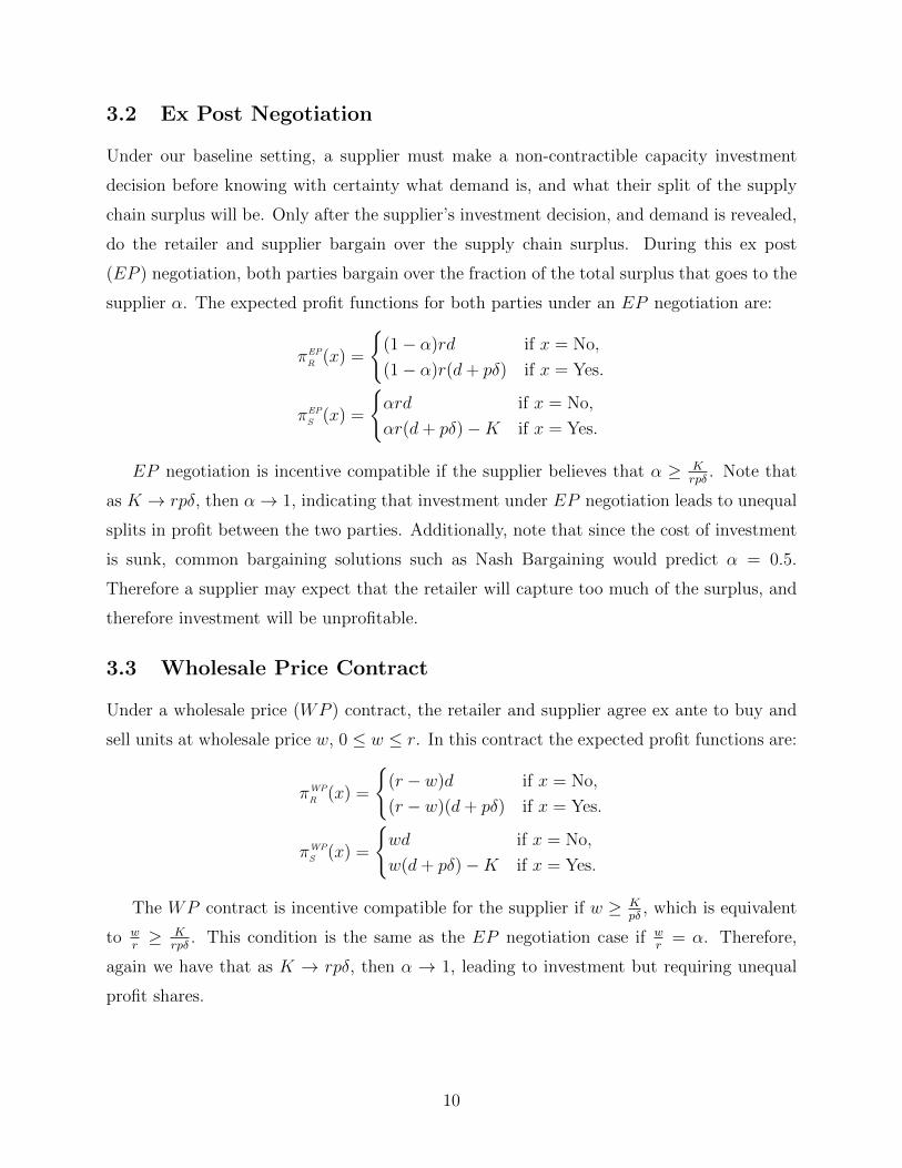
3.2 Ex Post Negotiation

Under our baseline setting, a supplier must make a non-contractible capacity investment

decision before knowing with certainty what demand is, and what their split of the supply

chain surplus will be. Only after the supplier’s investment decision, and demand is revealed,

do the retailer and supplier bargain over the supply chain surplus. During this ex post

(EP ) negotiation, both parties bargain over the fraction of the total surplus that goes to the

supplier α. The expected profit functions for both parties under an EP negotiation are:

πEP

R (x) =

{(1− α)rd if x = No,

(1− α)r(d+ pδ) if x = Yes.

πEP

S (x) =

{αrd if x = No,

αr(d+ pδ)−K if x = Yes.

EP negotiation is incentive compatible if the supplier believes that α ≥ Krpδ

. Note that

as K → rpδ, then α→ 1, indicating that investment under EP negotiation leads to unequal

splits in profit between the two parties. Additionally, note that since the cost of investment

is sunk, common bargaining solutions such as Nash Bargaining would predict α = 0.5.

Therefore a supplier may expect that the retailer will capture too much of the surplus, and

therefore investment will be unprofitable.

3.3 Wholesale Price Contract

Under a wholesale price (WP ) contract, the retailer and supplier agree ex ante to buy and

sell units at wholesale price w, 0 ≤ w ≤ r. In this contract the expected profit functions are:

πWP

R (x) =

{(r − w)d if x = No,

(r − w)(d+ pδ) if x = Yes.

πWP

S (x) =

{wd if x = No,

w(d+ pδ)−K if x = Yes.

The WP contract is incentive compatible for the supplier if w ≥ Kpδ

, which is equivalent

to wr≥ K

rpδ. This condition is the same as the EP negotiation case if w

r= α. Therefore,

again we have that as K → rpδ, then α → 1, leading to investment but requiring unequal

profit shares.

10

3.4 Quantity Premium Contract

A quantity premium (QP ) contract states that the retailer and supplier agree ex ante to buy

and sell units at wholesale price w1, 0 ≤ w1 ≤ r for the first d units, and wholesale price w2,

0 ≤ w2 ≤ r for the any units sold above d. In this contract the expected profit functions are:

πQP

R (x) =

{(r − w1)d if x = No,

(r − w1)d+ (r − w2)pδ if x = Yes.

πQP

S (x) =

{w1d if x = No,

w1d+ w2pδ −K if x = Yes.

The QP contract is incentive compatible when w2 ≥ Kpδ

= w2. There are a range of pos-

sible QP contracts that are both incentive compatible and give both parties equal expected

profit, specifically:12{w2 =

(r − 2w1)d+ rpδ +K

2pδ,r(d− pδ) +K

2d≤ w1 ≤

r(d+ pδ)−K2d

}.

3.5 Quantity Commitment Contract

Under a quantity commitment (QC) contract the retailer and supplier agree ex ante to buy

and sell units at a wholesale price of w, 0 ≤ w ≤ r, with a (binding) commitment that the

retailer buy at least q, d ≤ q ≤ D units. If the supplier does not invest, and is therefore

unable to deliver q units, then the retailer is released from the commitment and is free to

order any amount. Since the transaction is verifiable (i.e. the order size and units delivered

are provable to a court), it is feasible to make the quantity commitment legally enforceable.

In this contract the expected profit functions are:

πQC

R (x) =


(1− p)(rd− wq) + p(r − w)D if x = Yes.

πQC

S (x) =

{wd if x = No,

w(q + p(D − q))−K if x = Yes.

The QC contract is incentive compatible when q ≥ w(d−pD)+Kw(1−p) = q. Again, there are a

12Please see section A.1 in the Appendix for details.

11

range of possible contracts that are incentive compatible and equalize expected profits:{q =

(r − 2w)pD + r(1− p)d+K

2w(1− p),

r(d+ pδ) +K

2D≤ w ≤ min

{r(d+ pδ)−K

2d,r(d+ pδ) +K

2(d+ pδ)

}}.

3.6 Option Contract

In the option (OP ) contract, the retailer and supplier agree ex ante to buy and sell units up

to D units at a wholesale price of w, 0 ≤ w ≤ r, and the retailer pays a lump sum option

fee po to the supplier. If the supplier cannot deliver a unit that the buyer has an option

for, he must return the option fee. We refer to this contract as an “option” contract to be

consistent with past literature, for example, Noldeke & Schmidt (1995) use this title as the

contract provides the supplier with the option to invest in capacity, and receive the option

fee.13 In this contract the expected profit functions are:

πOP

R (x) =


(r − w)(d+ pδ)− po if x = Yes.

πOP

S (x) =

{wd if x = No,

w(d+ pδ) + po −K if x = Yes.

The OP contract is incentive compatible when po ≥ (K − wpδ) = po.14 Then, the set of

option contracts that are incentive compatible and equalizes expected profits are:{po =

(r − 2w)(d+ pδ) +K

2, w ≤ min

{r(d+ pδ)−K

2d,r(d+ pδ) +K

2(d+ pδ)

}}.

4. Experimental Design

The laboratory experiment was designed to study how different contracts, with structured

communication, affect capacity investment decisions. We evaluated the classic EP nego-

tiation case, along with each of the four contracts outlined in Section 3, in five separate

13Additionally, this can also be thought of as a more traditional options contract, where the retailer buysq ≤ D individual options for an option price of po/q. The options give the retailer the right to buy up to qunits at price w. If the retailer exercises more units than the supplier can deliver, the supplier must refundthe full option fee po. Note that we consider a simplified structure by fixing the number of options at q = D.

14We will consider an alternative form of the OP contract, where the investment is only observable ifdemand is high and the supplier neglects to invest in capacity, much like a service-level agreement, in arobustness check in Section 6.1.

12

treatments. Below we will outline the decision sequence of each treatment, followed by our

experimental parameters and predictions, and then detail our structured communication

protocol.

4.1 Experimental Sequence

Each treatment consisted of 10 rounds, where the decision sequence in each round differed

between the EP negotiation treatment, and the four contract treatments (please refer to

Figure 1). In each round of the EP treatment, a participant was first randomly assigned the

role of a retailer or supplier. They were then randomly matched, anonymously, with someone

of the opposite role. The supplier then made a decision of whether to incur a fixed cost to

invest in capacity. After this, random demand was realized, and the supply chain surplus,

along with the supplier’s investment decision, was displayed to both parties. The retailer

and supplier then bargained over the split of the supply chain surplus. If an agreement was

reached on the split of the supply chain surplus, both parties earned their respective private

profits and the round ended.

Supplier investment

decision

Preliminary results: demand,

supplier’s decision, surplus

Bargaining overα

Final results

Role assignment

Ex Post Negotiation

(EP)

Supplier’s investment

decision

Bargaining over w

Final results

Role assignment

WholesalePrice(WP)


decision

Bargaining over w1, w2

Final results

Role assignment

Quantity Premium

(QP)


decision

Bargaining over w, q

Final results

Role assignment

Quantity Commitment

(QC)


decision

Bargaining over w, po

Final results

Role assignment

Option(OP)

Figure 1: Decision sequence in each of the experimental treatments.

13

In the four contract treatments, as with the EP treatment, each round began with a

participant being randomly assigned the role of a retailer or supplier, who was then matched

randomly with someone of the opposite role. However, unlike the EP treatment, following

the role assignment and matching, the pair then began to bargain over the appropriate con-

tract parameter(s). In the WP contract, the retailer and supplier bargained over a wholesale

price, in the QP contract they bargained over two wholesale prices simultaneously, in the

QC contract they bargained over a wholesale price and quantity commitment simultane-

ously, and in the OP contract they bargained over a wholesale price and option payment

simultaneously. After an agreement was reached in this bargaining stage, the supplier then

made the decision of whether to incur a fixed cost and invest in capacity. Lastly, random

demand was realized, and the appropriate profits were displayed privately to each player to

end the round.

4.2 Experimental Parameters and Predictions

We used the same experimental parameters in all treatments. Following the theory outlined

in Section 3, we set demand to follow a two-point distribution, with high demand D = 20

and low demand d = 10, where the probability of high demand was p = 12. The supplier’s

investment cost was set to K = 35, allowing them to increase their capacity from d = 10

units to D = 20 units. The retailer’s revenue per unit was r = 10, and the supplier’s marginal

cost per unit was c = 0.

Given these experimental parameters, if the supplier does not decide to invest in capacity,

then the total supply chain surplus and profit is 100. If the supplier does choose to incur

the investment cost and increase capacity, then the expected supply chain surplus is 150 =

r(d + pδ), and the total expected supply chain profit is 115 = r(d + pδ) −K. This means

that underinvestment leads to an expected profit reduction of 15 = (115− 100).

There were 38 participants in the EP treatment, and 48 participants in each of the four

contract treatments, for a total of 230 subjects. Based on our experimental parameters

and the theory outlined in Section 3, one can calculate contract parameters necessary for

investment to be incentive compatible and equalize expected profits. This information is

shown in Table 1.

15IC contracts make up 30% of the individually rational contracting space for WP and QP , 44% for QC,and 84% for OP .

14

Table 1: Experimental design, number of participating subjects, and contract details.

Participants Incentive Compatible15 Equal Profits | Incentive Compatible

EP 38 α ≥ 0.70 -

WP 48 w ≥ 7.00 -

QP 48 w2 ≥ 7.00 {w2 = (18.5− 2w1), 4.25 ≤ w1 ≤ 5.75}QC 48 q ≥ 70

w{q =

(185w− 20

), 4.63 ≤ w ≤ 5.75}

OP 48 po ≥ (35− 5w) {po = (92.5− 15w), w ≤ 5.75}

As mentioned previously, it is important to note that EP negotiation and the WP

contract can only induce investment for highly unequal expected profit splits, but the three

other contracts can all induce investment with equal expected profit splits.

We conducted all sessions at a large northeastern university in the fall of 2012 and spring

of 2013. Subjects in all treatments were students, mostly undergraduates. Before each

session subjects read the instructions themselves. Following this, we read the instructions

out loud and answered any questions. In total, roughly 30 minutes were spent reviewing

the details of the game. We recruited participants through an online recruitment system

where cash was the only incentive offered. Subjects were paid a $5 show-up fee plus an

additional amount that was based on their personal performance for all 10 rounds. Average

compensation for the participants, including the show-up fee, was just over $26. Each session

lasted approximately 90 minutes, and we programmed the experimental interface using zTree

(Fischbacher 2007).

4.3 Structured Communication Protocol

As mentioned in Section 2, experimentally studying bargaining in a controlled laboratory

setting typically involves one of two extremes; ultimatum take-it-or-leave-it offers or free

form negotiation. For our experiment we developed a structured communication protocol

that permitted players to bargain with each other dynamically, thus allowing allowing us

to monitor how contract offers evolved over time. The bargaining stage in each round of

each treatment lasted for four minutes.16 Consider the QC contract as an example. During

this time, a retailer and supplier would bargain simultaneously over a wholesale price and

quantity commitment amount. Both players could propose different combinations of the

16The data, and informal conversations with participants, indicates that four minutes was a sufficientamount of time for participants to get comfortable with the interface and explore the parameter spaces.

15

wholesale price and quantity commitment at any point in time, with no restrictions on the

number of offers, and no rules requiring alternating offers (i.e. a subject could make as many

offers in a row without the other player responding).

When either player received an offer, they could either accept it, or, provide feedback to

the proposer with respect to the contract parameters.17 For instance, in the QC contract,

someone receiving an offer could let the proposer know whether they felt wholesale price was

too high or too low, and/or whether they felt that the quantity commitment was too high

or too low. To help subjects keep track of their proposed and received contract offers, we

also provided them with two tables, which displayed all of the past proposed and received

contract offers, along with any feedback (i.e. if a contract parameter was too high or low).

If either party chose to accept a contract proposal at any time, the bargaining stage ended.

Alternatively, if an agreement was not reached, both parties earned an outside option profit

of zero. We provide a detailed screenshot of the QC bargaining stage in section A.4 in the

Appendix. By utilizing this type of bargaining structure, we emulated a process that incor-

porates important features of a realistic negotiation process (i.e. dynamic offers, feedback,

etc), while maintaining our ability to directly monitor the bargaining dynamics.

5. Results

5.1 Contract Performance

Retailer-supplier dyads successfully reached an agreement at similar rates across all five treat-

ments. Results of a series of two-sided proportions tests reveals only one significant difference

in agreement rates, between the WP contract (81% agreement) and the QC contract (92%

agreement). Therefore, we first focus on investment rates and contract parameters given

agreements, and later explore offers that were not accepted when we present the bargaining

dynamics, in the subsequent section.

Figure 2 depicts the average investment rates by suppliers for each treatment. As one can

see in the first column of Figure 2, while the average investment rate in the EP negotiation

treatment is significantly higher than 0%, supplier investment only occurs 29.70% of the

time, leading to a substantial reduction in potential profits

Continuing with Figure 2, a two-sided proportions test, with an individual represent-

ing an independent observation, reveals that investment rates in the WP contract are not

17Subjects were only allowed to accept or provide feedback on the latest offer received.

16

QP QC OP

vest

Invest

0%

20%

40%

60%

80%

100%

EP WP QP QC OP

29.70% 35.38%

43.26% 51.58%

86.85%

0%

20%

40%

60%

80%

100%

EP WP QP QC OP

Inve

stm

ent R

ate

Figure 2: Average investment rates for each experimental treatment.

significantly higher than in the EP treatment (p = 0.3298). This is somewhat expected,

as the WP contract can only induce the supplier to invest in capacity if there are highly

unequal splits in expected profits between the two parties. However, when comparing the

QP contract to the EP negotiation treatment, we again observe no significant difference

in average investment rates (p = 0.1657). This is contrary to the normative theory, which

shows that the QP contract can not only induce investment, but also lead to an equitable

split of profits.

A different result emerges when we compare the QC and OP contracts to the baseline

EP negotiation treatment. In both the QC contract and OP contract, investment levels

are significantly higher than the EP case (p = 0.023 in the QC contract, and p < 0.001

in the OP contract). This is especially true in the OP contract. It achieves an average

investment rate of 86.85%. Not only is this investment rate higher than the baseline EP

negotiation case, but it is also significantly higher than each of the other three contracts (all

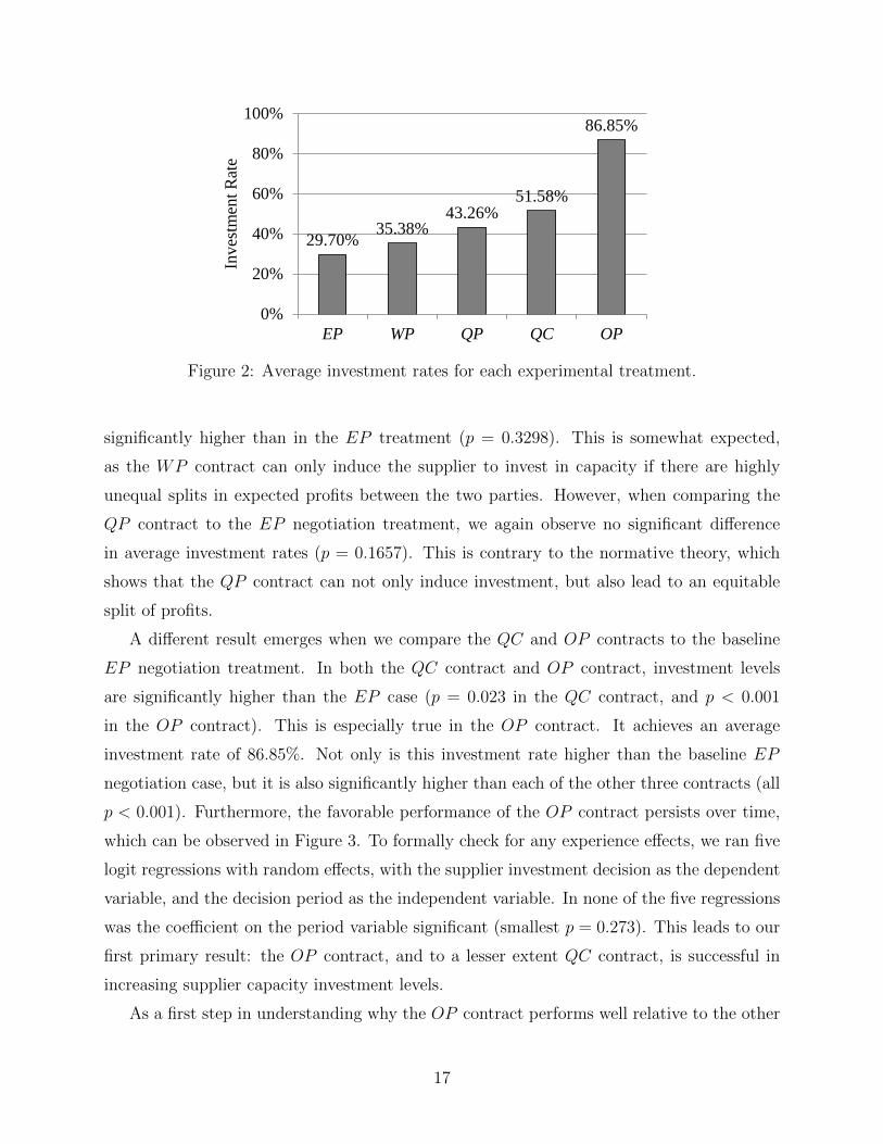
p < 0.001). Furthermore, the favorable performance of the OP contract persists over time,

which can be observed in Figure 3. To formally check for any experience effects, we ran five

logit regressions with random effects, with the supplier investment decision as the dependent

variable, and the decision period as the independent variable. In none of the five regressions

was the coefficient on the period variable significant (smallest p = 0.273). This leads to our

first primary result: the OP contract, and to a lesser extent QC contract, is successful in

increasing supplier capacity investment levels.

As a first step in understanding why the OP contract performs well relative to the other

17

9 10 1 2 3 4 5 6 7

103.75 105 26% 29% 64% 18% 38% 25% 25%104.5652 104.6154 52% 42% 24% 30% 29% 36% 33%106.8182 108.6842 35% 54% 45% 50% 48% 35% 27%107.1429 106.4286 45% 64% 50% 57% 52% 65% 43%112.8571 112.1429 86% 90% 92% 90% 85% 91% 83%

earnings20132.425209.6

2695225641.6

26394.24Tl less 5 123179.8

5355.645game earn 23.28541end 28.28541

0%

20%

40%

60%

80%

100%

1 2 3 4 5 6 7 8 9 10

Inve

stm

ent R

ate

Period

EPWPQPQCOP

Figure 3: Average investment rates over time for each experimental treatment.

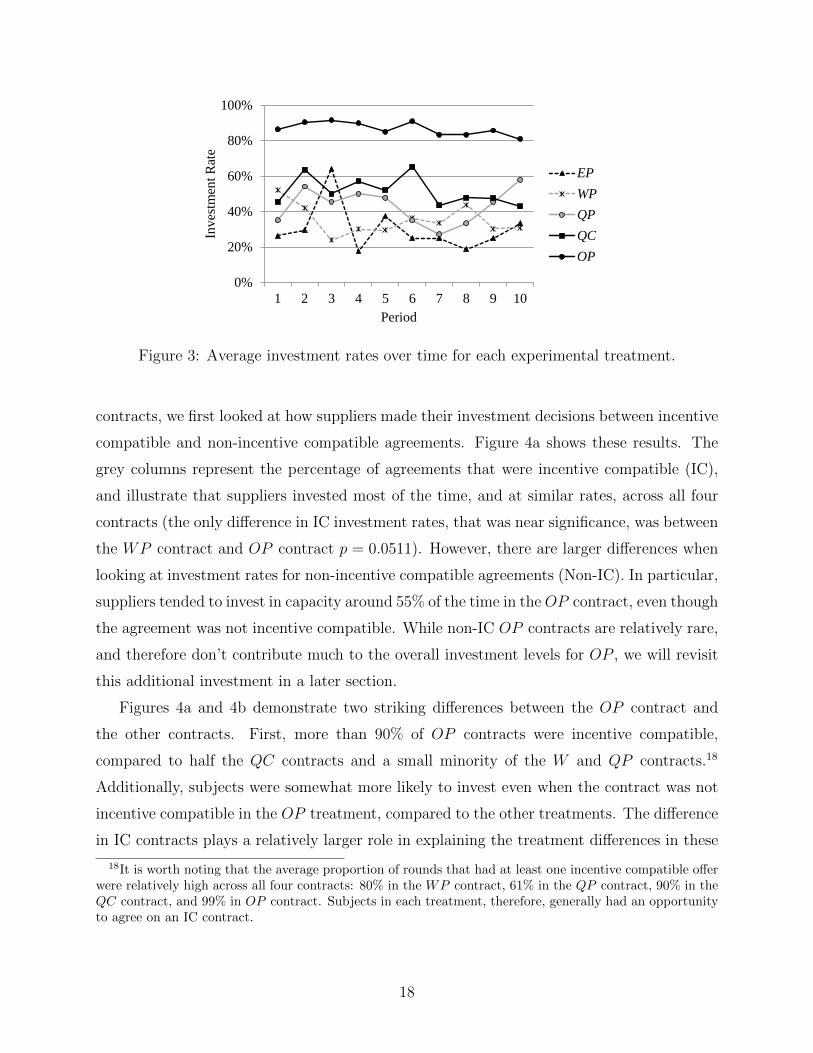
contracts, we first looked at how suppliers made their investment decisions between incentive

compatible and non-incentive compatible agreements. Figure 4a shows these results. The

grey columns represent the percentage of agreements that were incentive compatible (IC),

and illustrate that suppliers invested most of the time, and at similar rates, across all four

contracts (the only difference in IC investment rates, that was near significance, was between

the WP contract and OP contract p = 0.0511). However, there are larger differences when

looking at investment rates for non-incentive compatible agreements (Non-IC). In particular,

suppliers tended to invest in capacity around 55% of the time in theOP contract, even though

the agreement was not incentive compatible. While non-IC OP contracts are relatively rare,

and therefore don’t contribute much to the overall investment levels for OP , we will revisit

this additional investment in a later section.

Figures 4a and 4b demonstrate two striking differences between the OP contract and

the other contracts. First, more than 90% of OP contracts were incentive compatible,

compared to half the QC contracts and a small minority of the W and QP contracts.18

Additionally, subjects were somewhat more likely to invest even when the contract was not

incentive compatible in the OP treatment, compared to the other treatments. The difference

in IC contracts plays a relatively larger role in explaining the treatment differences in these

18It is worth noting that the average proportion of rounds that had at least one incentive compatible offerwere relatively high across all four contracts: 80% in the WP contract, 61% in the QP contract, 90% in theQC contract, and 99% in OP contract. Subjects in each treatment, therefore, generally had an opportunityto agree on an IC contract.

18

(1) (2) (3) (4)VARIABLE invest invest invest invest

isIC 0.424*** 0.542*** 0.547*** 0.346***(0.106) (0.0718) (0.0694) (0.115)

period -0.00351 -0.0110 -0.00285 -0.00947(0.0102) (0.0110) (0.00911) (0.00718)

Constant 0.323*** 0.374*** 0.254*** 0.603***(0.0736) (0.0736) (0.0724) (0.114)

Observatio 195 215 221 213Number of 48 48 48 47Robust sta *** p<0.01,

QC OP

Non-IC

IC

0%

20%

40%

60%

80%

100%

WP QP QC OP

Inve

stm

ent R

ates

Non-IC IC

0%

20%

40%

60%

80%

100%

WP QP QC OP

Inve

stm

ent R

ates

Non-ICIC

(a) Investment Rates

OP

% IC

0%

20%

40%

60%

80%

100%

WP QP QC OP

Ince

ntiv

e C

ompa

tible

Rat

es

(b) IC Offers

Figure 4: Figure 4a shows average investment rates for non-incentive compatible (Non-IC)agreements, and investment rates for incentive compatible agreements (IC). Figure 4b showsthe average rate of incentive compatible agreements across all four contracts.

sessions19, however the excess investment under non-IC contracts will play a larger role (and

be discussed further) in the additional treatments we run in Section 6.

Table 2 delineates the average contract parameters for agreements in each experimental

treatment, as well as the expected share of the surplus the contract assigns to the supplier.

Additionally, the last column shows the average required condition on the second term of the

contract for incentive compatibility, given the observed wholesale price. Starting with the

EP negotiation treatment, retailers and suppliers agreed on a near 50-50 split in dividing

the supply chain surplus (50.58% going to the supplier). Recall from our experimental

predictions, in Table 1, that under EP negotiation, the supplier must expect to receive at

least 70% of the supply chain surplus in order for investment to be worthwhile. Therefore,

the lack of investment observed in the EP negotiation case is expected given the agreements.

Moving to theWP contract, the average agreed upon price was 5.61, again below the required

19To assess the relative impact of contract composition and investment decisions, for each treatment wecalculate what the investment rate would be if the fraction of IC contracts matched the OP treatment(keeping fixed the investment decision conditional on incentive compatibility), and what it would be if theinvestment decisions conditional on contract incentives matched the OP contract (keeping fixed the percentof IC contracts). For the QC treatment making either of these changed would eliminate approximatelytwo-thirds of the difference in overall investment rates. For QP changing the share of IC contracts closes85% of the gap, while changing the investment decisions shrinks the gap by 45%. For W changing the shareof IC contracts reduces the treatment difference by 65%, while changing the investment decisions reducesthe difference by half. In all cases the share of IC contracts plays as big or bigger role in the treatmentdifferences than the investment decisions.

19

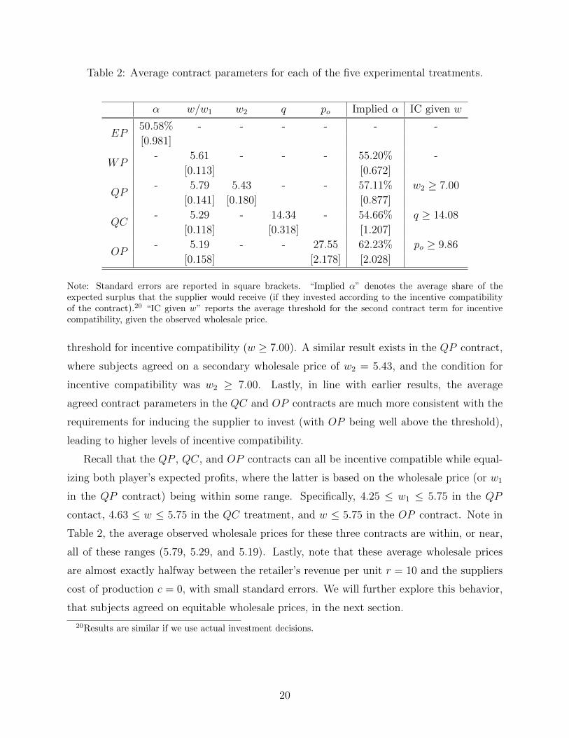
Table 2: Average contract parameters for each of the five experimental treatments.

α w/w1 w2 q po Implied α IC given w

EP50.58% - - - - - -

[0.981]

WP- 5.61 - - - 55.20% -

[0.113] [0.672]

QP- 5.79 5.43 - - 57.11% w2 ≥ 7.00

[0.141] [0.180] [0.877]

QC- 5.29 - 14.34 - 54.66% q ≥ 14.08

[0.118] [0.318] [1.207]

OP- 5.19 - - 27.55 62.23% po ≥ 9.86

[0.158] [2.178] [2.028]

Note: Standard errors are reported in square brackets. “Implied α” denotes the average share of theexpected surplus that the supplier would receive (if they invested according to the incentive compatibilityof the contract).20 “IC given w” reports the average threshold for the second contract term for incentivecompatibility, given the observed wholesale price.

threshold for incentive compatibility (w ≥ 7.00). A similar result exists in the QP contract,

where subjects agreed on a secondary wholesale price of w2 = 5.43, and the condition for

incentive compatibility was w2 ≥ 7.00. Lastly, in line with earlier results, the average

agreed contract parameters in the QC and OP contracts are much more consistent with the

requirements for inducing the supplier to invest (with OP being well above the threshold),

leading to higher levels of incentive compatibility.

Recall that the QP , QC, and OP contracts can all be incentive compatible while equal-

izing both player’s expected profits, where the latter is based on the wholesale price (or w1

in the QP contract) being within some range. Specifically, 4.25 ≤ w1 ≤ 5.75 in the QP

contact, 4.63 ≤ w ≤ 5.75 in the QC treatment, and w ≤ 5.75 in the OP contract. Note in

Table 2, the average observed wholesale prices for these three contracts are within, or near,

all of these ranges (5.79, 5.29, and 5.19). Lastly, note that these average wholesale prices

are almost exactly halfway between the retailer’s revenue per unit r = 10 and the suppliers

cost of production c = 0, with small standard errors. We will further explore this behavior,

that subjects agreed on equitable wholesale prices, in the next section.

20Results are similar if we use actual investment decisions.

20

5.2 Bargaining Dynamics

Across all contracts, over time, the evolution of contract proposals changed considerably.

In Figure 5, we provide six sunflower density plots, two for each of the QP , QC, and OP

contracts. These density plots represent the contract proposals during the bargaining stage

at different moments in time. Specifically, the left-hand side figures show the density of

contract offers during the first two minutes of bargaining (first half), whereas the right-hand

side figures show the density of contract offers during the last two minutes of bargaining

(second half). In all six plots, the vertical axis denotes the wholesale price (w1 in the QP

contract), and the horizontal axis represents the other, coordinating, contract parameter.

One can immediately notice that the change in contract proposals, from the first to second

half, is similar across all three contracts. Specifically, during the first half of bargaining,

there is considerable dispersion of offers for both parameters. However, during the final

half of bargaining, wholesale prices converge to around 5.00, whereas the second parameter

continues to have considerable variability.

21

02

46

810

w1

0 2 4 6 8 10w2

1 petal = 1 obs. 1 petal = 6 obs.

(a) QP first half

02

46

810

w1

0 2 4 6 8 10w2


(b) QP second half

02

46

810

w

10 12 14 16 18 20q


(c) QC first half

02

46

810

w

10 12 14 16 18 20q


(d) QC second half

02

46

810

w

0 50 100 150 200po


(e) OP first half

02

46

810

w

0 50 100 150 200po


(f) OP second half

Figure 5: Sunflower density plots for contract offers. Each circle represents a single obser-vation. Each line on a lightly-shaded hexagon represents one observation. Each line on adarkly-shaded hexagon represents six observations. The three left-hand side figures representcontract offers made during the first two minutes of bargaining (first half). The right-handside figures represent contract offers made during the last two minutes of bargaining (secondhalf). 22

Recall that our bargaining protocol not only allowed us to only track contract offers,

but also the feedback with respect these contract offers (i.e. whether a parameter was too

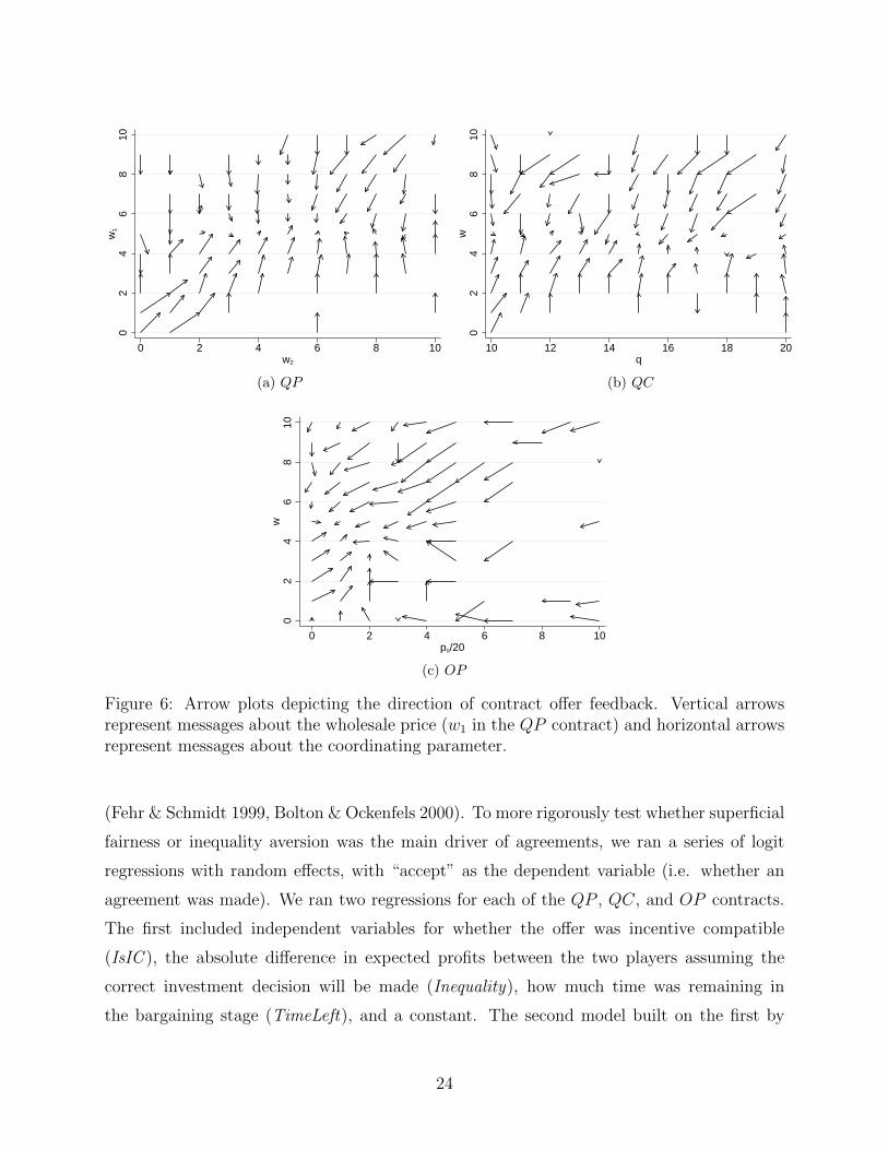
high or low). In Figure 6, we display three arrow plots that illustrate the types of feedback

sent for contract offers, one for each of the QP , QC, and OP contracts. The vertical axis

represents the wholesale price (w1 for the QP contract) and the horizontal axis represents

the coordinating parameter. For instance, take Figure 6b, which denotes the message types

sent in the QC treatment. The majority of the arrows are vertical, which means that most

of the messages were with regard to the wholesale price being too high (down arrow) or too

low (up arrow). In fact, in both the QC and QP contract, a vast majority of the messages

focused on driving the wholesale price to around 5.00. In the OP contract, this effect is not

quite as strong. However, if one excludes the larger option payments, such as po < 40, which

often are irrational for the retailer to accept (depending on the wholesale price) then again,

most of the messages are aimed at pushing the wholesale price to somewhere in the middle

of the revenue per unit r = 10 and cost per unit c = 0.

While it appears that participants appear to focus more on the wholesale price than the

coordinating parameter, it is also possible that they attempted to establish the wholesale

price first, and once they agreed on it, they then bargained over the coordinating parameter.

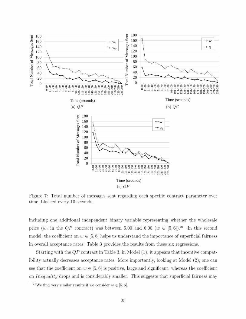
Therefore, in Figure 7, we plot the total number of messages sent, over time and blocked

every 10 seconds, for each contract parameter. Looking at this figure we can make a few

observations. First, in all three contracts, there are less messages for both parameters as

time proceeded. Second, there are consistently more messages about the wholesale price than

the coordinating parameter, even towards the end of the bargaining time, for all contracts.

And third, the difference between the number of messages sent about the wholesale price

and the coordinating parameter is much smaller in the OP contract. Additionally, while

not depicted, we also checked for other indications that subjects were taking a sequential

process to the two contact parameters. For example, we checked the number of changes in

each contract parameter over time, or the percentage change in each contract parameter over

time, and continue to find that subjects bargain and alter both contract terms simultaneously

over time, with more emphasis on the wholesale price.

Thus far, the experimental results and bargaining dynamics show that participants focus

primarily on setting an equitable wholesale price. We will refer to this behavior as “superficial

fairness.” That said, another potential explanation for the bargaining behavioral is that

subjects were concerned about true inequality aversion with respect to their expected profits

23

02

46

810

w1

0 2 4 6 8 10w2

(a) QP

02

46

810

w

10 12 14 16 18 20q

(b) QC

02

46

810

w

0 2 4 6 8 10po/20

(c) OP

Figure 6: Arrow plots depicting the direction of contract offer feedback. Vertical arrowsrepresent messages about the wholesale price (w1 in the QP contract) and horizontal arrowsrepresent messages about the coordinating parameter.

(Fehr & Schmidt 1999, Bolton & Ockenfels 2000). To more rigorously test whether superficial

fairness or inequality aversion was the main driver of agreements, we ran a series of logit

regressions with random effects, with “accept” as the dependent variable (i.e. whether an

agreement was made). We ran two regressions for each of the QP , QC, and OP contracts.

The first included independent variables for whether the offer was incentive compatible

(IsIC ), the absolute difference in expected profits between the two players assuming the

correct investment decision will be made (Inequality), how much time was remaining in

the bargaining stage (TimeLeft), and a constant. The second model built on the first by

24

020406080

100120140160180

0-10

11-2

021

-30

31-4

041

-50

51-6

061

-70

71-8

081

-90

91-1

0010

1-11

011

1-12

012

1-13

013

1-14

014

1-15

015

1-16

016

1-17

017

1-18

018

1-19

019

1-20

020

1-21

021

1-22

022

1-23

023

1-24

0Tota

l Num

ber o

f Mes

sage

s Sen

t

Time (seconds)

w1w2w1

w2

(a) QP

020406080

100120140160180

0-10

11-2

021

-30

31-4

041

-50

51-6

061

-70

71-8

081

-90

91-1

0010

1-11

011

1-12

012

1-13

013

1-14

014

1-15

015

1-16

016

1-17

017

1-18

018

1-19

019

1-20

020

1-21

021

1-22

022

1-23

023

1-24

0Tota

l Num

ber o

f Mes

sage

s Sen

t

Time (seconds)

wq

(b) QC

020406080

100120140160180

0-10

11-2

021

-30

31-4

041

-50

51-6

061

-70

71-8

081

-90

91-1

0010

1-11

011

1-12

012

1-13

013

1-14

014

1-15

015

1-16

016

1-17

017

1-18

018

1-19

019

1-20

020

1-21

021

1-22

022

1-23

023

1-24

0Tota

l Num

ber o

f Mes

sage

s Sen

t

Time (seconds)

wpp0

(c) OP

Figure 7: Total number of messages sent regarding each specific contract parameter overtime, blocked every 10 seconds.

including one additional independent binary variable representing whether the wholesale

price (w1 in the QP contract) was between 5.00 and 6.00 (w ∈ [5, 6]).21 In this second

model, the coefficient on w ∈ [5, 6] helps us understand the importance of superficial fairness

in overall acceptance rates. Table 3 provides the results from these six regressions.

Starting with the QP contract in Table 3, in Model (1), it appears that incentive compat-

ibility actually decreases acceptance rates. More importantly, looking at Model (2), one can

see that the coefficient on w ∈ [5, 6] is positive, large and significant, whereas the coefficient

on Inequality drops and is considerably smaller. This suggests that superficial fairness may

21We find very similar results if we consider w ∈ [5, 6].

25

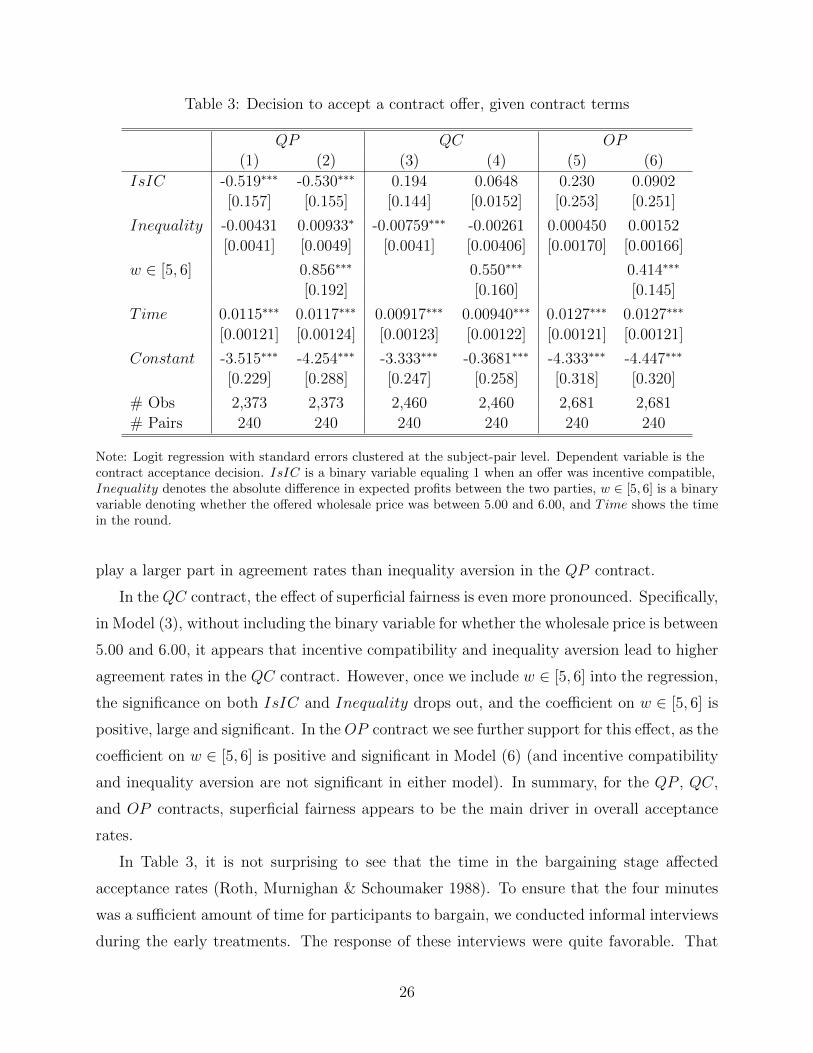
Table 3: Decision to accept a contract offer, given contract terms

QP QC OP

(1) (2) (3) (4) (5) (6)

IsIC -0.519∗∗∗ -0.530∗∗∗ 0.194 0.0648 0.230 0.0902

[0.157] [0.155] [0.144] [0.0152] [0.253] [0.251]

Inequality -0.00431 0.00933∗ -0.00759∗∗∗ -0.00261 0.000450 0.00152

[0.0041] [0.0049] [0.0041] [0.00406] [0.00170] [0.00166]

w ∈ [5, 6] 0.856∗∗∗ 0.550∗∗∗ 0.414∗∗∗

[0.192] [0.160] [0.145]

Time 0.0115∗∗∗ 0.0117∗∗∗ 0.00917∗∗∗ 0.00940∗∗∗ 0.0127∗∗∗ 0.0127∗∗∗

[0.00121] [0.00124] [0.00123] [0.00122] [0.00121] [0.00121]

Constant -3.515∗∗∗ -4.254∗∗∗ -3.333∗∗∗ -0.3681∗∗∗ -4.333∗∗∗ -4.447∗∗∗

[0.229] [0.288] [0.247] [0.258] [0.318] [0.320]

# Obs 2,373 2,373 2,460 2,460 2,681 2,681

# Pairs 240 240 240 240 240 240

Note: Logit regression with standard errors clustered at the subject-pair level. Dependent variable is thecontract acceptance decision. IsIC is a binary variable equaling 1 when an offer was incentive compatible,Inequality denotes the absolute difference in expected profits between the two parties, w ∈ [5, 6] is a binaryvariable denoting whether the offered wholesale price was between 5.00 and 6.00, and Time shows the timein the round.

play a larger part in agreement rates than inequality aversion in the QP contract.

In the QC contract, the effect of superficial fairness is even more pronounced. Specifically,

in Model (3), without including the binary variable for whether the wholesale price is between

5.00 and 6.00, it appears that incentive compatibility and inequality aversion lead to higher

agreement rates in the QC contract. However, once we include w ∈ [5, 6] into the regression,

the significance on both IsIC and Inequality drops out, and the coefficient on w ∈ [5, 6] is

positive, large and significant. In the OP contract we see further support for this effect, as the

coefficient on w ∈ [5, 6] is positive and significant in Model (6) (and incentive compatibility

and inequality aversion are not significant in either model). In summary, for the QP , QC,

and OP contracts, superficial fairness appears to be the main driver in overall acceptance

rates.

In Table 3, it is not surprising to see that the time in the bargaining stage affected

acceptance rates (Roth, Murnighan & Schoumaker 1988). To ensure that the four minutes

was a sufficient amount of time for participants to bargain, we conducted informal interviews

during the early treatments. The response of these interviews were quite favorable. That

26

said, the timing of agreements agrees with this. The average time it took to come to an

agreement was just over two minutes in the EP negotiation treatment, and around three

minutes in the contract treatments (the longest was the WP contract, which took three

minutes 10 seconds on average). This implies not only that the time to bargain was sufficient,

but that the subjects also took the task seriously.22

5.2.1 The Impact of Superficial Fairness

Thus far, we have shown that agreements between retailers and suppliers are mainly driven

by superficial fairness. Here we show that this behavior can also explain our primary ex-

perimental result: that the OP , and to a lesser extent QC, contract is most successful at

increasing supplier capacity investment levels.

As shown in Section 3, when both contract parameters are unconstrained, the QP , QC,

and OP contracts are equivalent in terms of incentive compatibility and allowing an equitable

distribution of profits. However, once one of the two parameters are restricted to a particular

value, the performance of these contracts may differ. If we consider superficial fairness, and

assume that the average wholesale price in all three contracts is w = 5.00, then the proportion

the contract space for the second parameter that will lead to incentive compatibility, greatly

differs across the contracts. For example, in the QC contract, the quantity commitment

parameter, by definition, must be between low demand and high demand (d = 10 ≤ q ≤D = 20), where the condition for incentive compatibility is q ≥ 70

w. If w = 5.00, the

requirement for incentive compatibility in the QC contract is then q ≥ 14, which means

that 60% of the quantity commitment parameter space, 20−1420−10

, leads to incentive compatible

outcomes. If we apply this same approach to each of the three contracts with two parameters,

we arrive at:

• QP : If w = 5.00, then w2 ≥ 7→ 30% of the contract space for w2,

• QC: If w = 5.00, then q ≥ 14→ 60% of the contract space for q,

22Furthermore, while we spent roughly 30 minutes in each treatment explaining the experiment, we alsochecked for signs in the data indicating that the subjects comprehended the task. In general, we found that (1)proposers initially made more favorable to themselves, and then compromised over time, (2) suppliers mademore incentive compatible offers than retailers, (3) responders tended to reject, or not accept, unfavorableoffers, and (4) roughly 55-60% of all offers were made by suppliers. All of these results imply that subjectshad a grasp of the experimental task.

27

• OP : If w = 5.00, then po ≥ 10→ 87% of the individual-rationality contract space for

po.23

In short, our data suggest that superficial fairness provides the OP contract, and to

a lesser extent the QC contract, a distinct advantage in arriving at incentive compatible

agreements, which in turn leads to higher investment rates and greater expected supply

chain profits.24 This is a general feature of our setup - in section A.3 in the Appendix

we demonstrate that for any set of parameters (that leads to a non-trivial capacity invest-

ment problem) the incentive compatible region for superficially fair contracts will always be

(weakly) largest for the OP contract.

6. Robustness Checks

Thus far we have shown that one plausible explanation for our data is the superficial fairness

hypothesis. In this section, we conduct three additional robustness checks, in out-of-sample

tests, and determine how well the superficial fairness hypothesis performs. In particular, we

conducted five additional treatments, constituting three robustness checks. The first of the

three robustness checks evaluates a new contract, a service-level agreement. The second,

reruns the original OP contract, but provides subjects with decision support showing their

expected profits both with and without investment for each offer made/received. And the

third, involves three new treatments where we alter the original experimental parameters.

For all three of these robustness checks we generate formal hypotheses using superficial

fairness, and test them using the data.

6.1 Robustness Check 1: Service-Level Agreement

In our original experiment we assumed that the supplier’s investment decision is observable

and therefore the retailer could force the supplier to forfeit the option fee whenever he did not

invest (not depending on the demand realization). This may give the OP contract a distinct

advantage over the other contracts, as it provides a very direct incentive for the supplier

to invest. However, as Cachon & Lariviere (2001) point out, capacity investments are not

23Any po > 75 actually generates negative expected profit for the retailer, despite being incentive compat-ible for supplier investment. Therefore, the 87% we report excludes any po > 75, and is a more conservativemetric.

24Additionally, note that the size of the IC region conditional on w = 5 is more informative in distinguishingbetween contracts than the size of the overall IC region discussed in Footnote 15.

28

always easy to observe. Therefore, we conducted an additional experimental treatment of

the OP contract where the investment is not directly observable. In this treatment, if

the supplier chooses not to invest, and demand is low, then they will still earn the option

payment. Conversely, if demand is high, then the supplier will forfeit the option payment.

This version of the option contract acts much like a service-level (SL) agreement, where the

retailer will reward the supplier whenever the supplier can satisfy demand.

We ran this new treatment with an additional 36 participants, using the same experimen-

tal parameters as before. If superficial fairness is present in the SL agreement, then w ≈ 5,

implying that po ≥ 20 → 73% of the individually rational contract space for po is incentive

compatible.

Hypothesis 1 If superficial fairness is present in the SL agreement, then the predicted or-

dering of incentive compatible agreements (and investment rates) is OP>SL>QC>QP>WP.

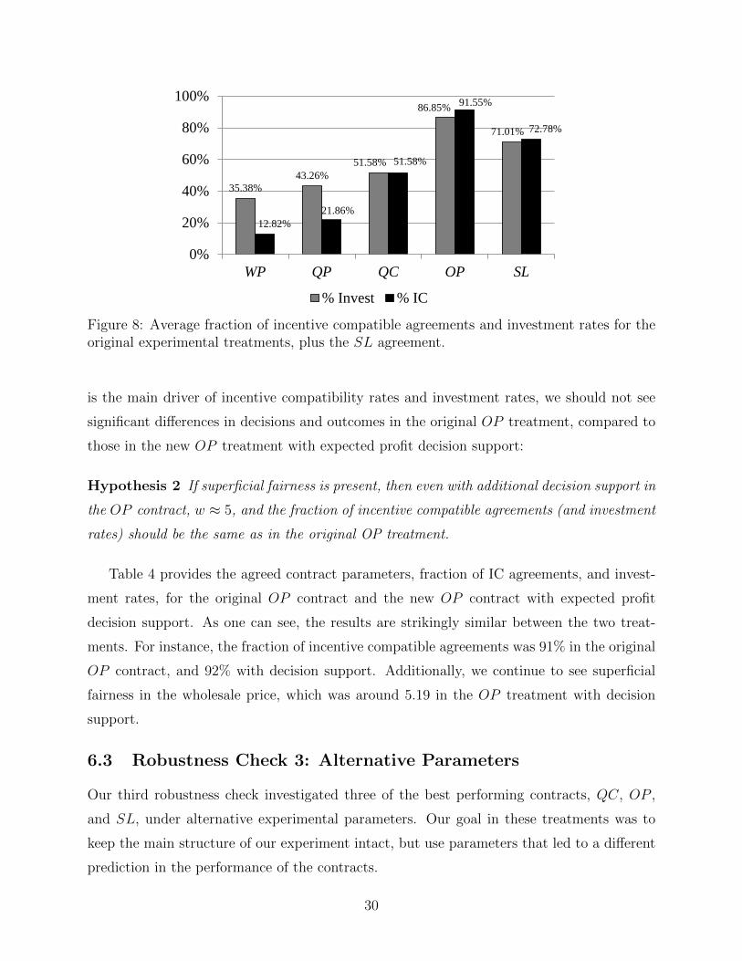
Figure 8 depicts the average fraction of incentive compatible agreements, and invest-

ment rates, for the original contract treatments, plus the SL agreement. As one can see,

the SL agreement’s fraction of incentive compatible agreements, and investment rates, are

below that of the OP contract, but above all other contracts. This is directly in line with

superficial fairness and Hypothesis 1. Additionally, the average wholesale price in the SL

treatment was 5.09, in line with superficial fairness. Finally, we note that, as with the origi-

nal OP contract, we find excess investment under non-incentive-compatible SL agreements.

Specifically, subjects invest 71% of the time when contracts are incentive compatible, and

65% of the time when contracts are not IC. Because of the relatively higher frequency of

non-IC contacts, these excess investments are now almost a quarter of the overall investment

decisions under the SL agreement.

6.2 Robustness Check 2: Decision Support

Our earlier results suggested that superficial fairness tends to be a more significant driver of

agreements than true fairness (in terms of expected profits). However, this is not entirely

surprising as our original treatments did not provide participants with the ability to see

what their potential expected profits were for each offer made or received. Therefore, in our

second robustness check, we reran the OP treatment, but whenever a participant made an

offer, we showed them their expected profits both with and without investment. Similarly,

when they received an offer, we showed them this same information. If superficial fairness

29

% InvestEP 29.70%WP 35.38%QP 43.26%QC 51.58%OP 86.85% 35.27%SL 71.01%

Subject Level Test of Proportionsp-value WP QP QC OptBase 0.3300 0.1700 0.0200 0.0000WP 0.6600 0.1600 0.0000QP 0.3300 0.0000QC 0.0000

(1)VARIABLES invest

Comparing Coefficients from Regression_Icontractt_2 0.0647 p-value WP QP QC Opt20

(0.0506) Base 0.201 0.012 0 0_Icontractt_3 0.136** WP 0.194 0.0055 0

(0.0542) QP 0.1525 0_Icontractt_4 0.222*** QC 0

(0.0558)_Icontractt_5 0.571***

(0.0438)period -0.00770

(0.00481)Constant 0.338***

(0.0426)

Observations 1009Number of subje 229Robust standard *** p<0.01, ** p<

0.00%

10.00%

20.00%

30.00%

40.00%

50.00%

60.00%

70.00%

80.00%

90.00%

100.00%

EP WP Q

% In

35.38% 43.26%

51.58%

86.85%

71.01%

12.82% 21.86%

51.58%

91.55%

72.78%

0%

20%

40%

60%

80%

100%

WP QP QC OP SL

% Invest % IC

Figure 8: Average fraction of incentive compatible agreements and investment rates for theoriginal experimental treatments, plus the SL agreement.

is the main driver of incentive compatibility rates and investment rates, we should not see

significant differences in decisions and outcomes in the original OP treatment, compared to

those in the new OP treatment with expected profit decision support:

Hypothesis 2 If superficial fairness is present, then even with additional decision support in

the OP contract, w ≈ 5, and the fraction of incentive compatible agreements (and investment

rates) should be the same as in the original OP treatment.

Table 4 provides the agreed contract parameters, fraction of IC agreements, and invest-

ment rates, for the original OP contract and the new OP contract with expected profit

decision support. As one can see, the results are strikingly similar between the two treat-

ments. For instance, the fraction of incentive compatible agreements was 91% in the original

OP contract, and 92% with decision support. Additionally, we continue to see superficial

fairness in the wholesale price, which was around 5.19 in the OP treatment with decision

support.

6.3 Robustness Check 3: Alternative Parameters

Our third robustness check investigated three of the best performing contracts, QC, OP ,

and SL, under alternative experimental parameters. Our goal in these treatments was to

keep the main structure of our experiment intact, but use parameters that led to a different

prediction in the performance of the contracts.

30

Table 4: Results from the original OP treatment, and OP treatment with expected profitdecision support.

Original Decision Support

OP OP

w 5.19 5.26

po 27.6 25.6

IC rate 92% 91%

Investment rate 77% 87%

In these new treatments, we changed the probability of high demand to p = 14, and

the retailer revenue to r = 20. If the superficial fairness hypothesis holds, then we should

see w ≈ 10, and a different ordering of fraction of incentive agreements (and investment

rates) compared to the original treatments. Specifically, we should now see that the QC

outperforms the SL agreement.25 The details are given below:

• QC: If w = 10.00, then q ≥ 11.3 → 86.7% of the contract space (originally 60%)

• OP : If w = 10.00, then po ≥ 10 → 90% of the IR contract space (originally 87%)

• SL: If w = 10.00, then po ≥ 40 → 68% of the IR contract space (originally 73%)

We can use these predictions to develop our third and final hypothesis:

Hypothesis 3 Under the new experimental parameters, if superficial fairness is present,

then the order of fraction of incentive compatible agreements (and investment rate) should

be OP > QC > SL.

The average wholesale prices in the QC, OP , and SL treatments were 10.19, 9.90, and

9.70, all close to the prediction of 10. Figure 9 illustrates the fraction of incentive compatible

agreements, and investment rates, for the QC, OP , and SL treatments with the new exper-

imental parameters. Turning first to the black columns, the fraction of incentive compatible

agreements, we see the same ordering as predicted by superficial fairness, OP > QC > SL.

Focusing on the investment rates in Figure 9, however, we see that this ordering is not as

expected. In particular, in the SL agreement, subjects tended to invest 66.67% of the time,

despite the fraction of incentive compatible agreements being only 38.89%.26 Specifically,

25Steve - note here about how we couldn’t get OP to be worse than anything else?26We can multiple sessions of all of these treatments, and the same overinvestment result, in the SL

treatment, is observed in all session.

31

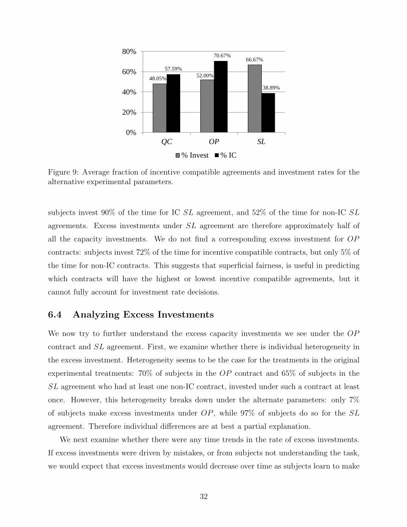
% Invest % ICQC 48.05% 57.59%OP 52.00% 70.67%SL 66.67% 38.89%

48.05% 52.00%

66.67%

57.59%

70.67%

38.89%

0%

20%

40%

60%

80%

QC OP SL

% Invest % IC

Figure 9: Average fraction of incentive compatible agreements and investment rates for thealternative experimental parameters.

subjects invest 90% of the time for IC SL agreement, and 52% of the time for non-IC SL

agreements. Excess investments under SL agreement are therefore approximately half of

all the capacity investments. We do not find a corresponding excess investment for OP

contracts: subjects invest 72% of the time for incentive compatible contracts, but only 5% of

the time for non-IC contracts. This suggests that superficial fairness, is useful in predicting

which contracts will have the highest or lowest incentive compatible agreements, but it

cannot fully account for investment rate decisions.

6.4 Analyzing Excess Investments

We now try to further understand the excess capacity investments we see under the OP

contract and SL agreement. First, we examine whether there is individual heterogeneity in

the excess investment. Heterogeneity seems to be the case for the treatments in the original

experimental treatments: 70% of subjects in the OP contract and 65% of subjects in the

SL agreement who had at least one non-IC contract, invested under such a contract at least

once. However, this heterogeneity breaks down under the alternate parameters: only 7%

of subjects make excess investments under OP , while 97% of subjects do so for the SL

agreement. Therefore individual differences are at best a partial explanation.

We next examine whether there were any time trends in the rate of excess investments.

If excess investments were driven by mistakes, or from subjects not understanding the task,

we would expect that excess investments would decrease over time as subjects learn to make

32

Table 5: Investment decisions for OP and SL treatments given contract terms.

r = 10 r = 20

OP SL OP SL

(1) (2) (3) (4) (5) (6) (7) (8)

IC Val 0.124*** 0.123*** 0.175*** 0.167***

[0.0313] [0.0391] [0.0205] [0.0327]

w 0.581** 0.204 0.407*** 0.306***

[0.270] [0.214] [0.140] [0.0879]

po 0.126*** 0.0968*** 0.174*** 0.0658***

[0.0336] [0.0261] [0.0206] [0.0126]

Constant 0.890*** -3.318** 0.753** -2.256 -1.340*** -7.158*** 1.215*** -4.297***

[0.328] [1.436] [0.300] [1.411] [0.256] [1.599] [0.220] [1.047]

# Obs 213 213 169 169 300 300 252 252

# Subjs 48 48 36 36 32 32 30 30

Note: Logit regression with subject random effects. Dependent variable is the investment decision.

IC Val denotes the net value of the incentive compatibility constraint, with positive values

indicating incentive compatibility; w and po are the wholesale price and option fee.

better decisions. However, we find no significant time trend for either contract under the

original parameters (non-parametric test for trends: OP p = 0.35; SL p = 0.13), or for OP

under the alternate parameters (p = 0.28). Indeed, we do find a significant increase in the

rate of excess investment over time for the SL agreement under the alternate parameters

(p = 0.01) - the excess investment rate is 45% in the first five periods, increasing to 61% in

the last five periods. Hence excess investment seems to represent a systematic bias, rather

than a transitory mistake.

Finally, we examine how investment decisions respond to the strength of financial incen-

tives in the contract. Table 5 reports the results of regressing a subject’s investment decision

on the overall financial incentives given the contract (odd columns), or the wholesale price

and option fee separately (even columns). As expected, subjects are more likely to invest

when the financial incentives to do so increase. While the coefficient on IC Val is largest for

the OP contract with r = 20, where we see the least excess investment, all of the coefficients

on IC Val are similar for all contracts and parameters. However, where we do see a difference

is in how subjects respond separately to the wholesale price and the option fee. Recall the

structure of the original problem: for the OP contract with r = 10, each dollar in wholesale

price provides the same incentives to the supplier as 5 dollars in option fee. Similarly, with

the OP contract and r = 20, each dollar of wholesale price provides the same incentives

as 2.5 dollars of option fee, and for SLA (for both r = 10 and r = 20) each dollar of

wholesale price is equivalent to 10 dollars of option fee. If subjects were correctly evaluating

33

the financial incentives of the contract, and basing their investment decisions on the overall

financial incentives, then the ratio of the estimated coefficients βw/βpo should match each

terms relative contribution to the overall incentives. We find that this is the case for the OP

contracts, but that subjects with SL agreements are substantially overvaluing the incentives

provided by the option fee (r = 10: βw/βpo = 2.11; r = 20: βw/βpo = 4.65). Hence, for

non-IC SL agreements with relatively high option fees, subjects are acting as if the contracts

provide more incentives than they actually do. This is consistent with our observation that

we find more excess investment under the SL agreement than the OP contract. One possible

explanation is to note that the option fee, unlike the wholesale price (or any of the other

coordinating terms), is paid to the supplier at the time of contracting, and the fee is forfeited

if the supplier does not invest. Hence the option fee may invoke loss aversion in a way that

the other contract terms do not. However, this mechanism should apply to both OP and

SL agreement, whereas we only see overweighting of the option fee for SL agreements.

7. Conclusion

We experimentally compare three contracts (quantity premium, quantity commitment and an

option contract) that, in theory, should each be able to solve a common capacity investment

problem, by generating investment incentives while equalizing the expected profits of the

retailer and supplier. We find that the option contract significantly outperforms the other

contracts, with the quantity premium contract providing no significant improvement over the

base case. We also find that while suppliers invest when doing so is incentive compatible,

there is a substantial difference, across contracts, in the frequency of incentive compatible

agreements.

The experimental design that we implement allows us to track and observe the bargaining

dynamics over time. Through this bargaining protocol, we observe that subjects, rather than

focusing on incentive compatibility or the true expected payoff differences, appear to have

preferences for “superficial fairness.” That is, subjects were heavily focused on ensuring

that the wholesale price was near the middle of the contracting space, while paying little

attention to the coordinating term. The option contract performs best in large part because

it is the most robust to this kind of superficial fairness, having the largest range of incentive

compatible coordinating terms, given a superficially fair wholesale price. We continue to see

that superficial fairness is present in a number of out-of-sample tests. Specifically, in settings

34

with other contract structures, additional decision support, and alternative parameters.This

focus on bargaining over one salient term is not uncommon in the bargaining literature -

often due to negotiators using sequential agendas that make joint gains hard to find (Mannix,

Thompson & Bazerman 1989), or by focusing on distributing value rather than finding

integrative solutions - the “mythical fixed pie” (Bazerman & Neale 1994). Similarly, Lovejoy

(2010) finds that it is quite common for supply chains managers to fix the order quantity

first, and then bargain on price. A second benefit of option-like contracts (include service

level agreements) is that in many cases these kinds of contracts lead to capacity investment

even when the financial terms of the contract do not provide sufficient incentives. Hence

these contracts can “outperform” their terms. We do not see this kind of excess investment

for the quantity premium and quantity commitment contracts.

There are several opportunities for future research in this area. One would be to extend

the work here, but in a repeated setting. As mentioned previously, repeated interaction

is a common solution to capacity investment problems, and would be an opportunity for

future research. Additionally, studies exploring alternative bargaining protocols could be

promising, such as comparing one-shot take-it-or-leave-it offers to structured communication

to free-form communication. Finally, additional research could further explore the excess

investment behavior we observed with option-like contracts.

One limitation of our study is the limited time subjects had to bargain. While it is

reasonable to expect that most supply chain negotiations would likely involve a greater

length of time, and some additional level of calculations for each offer, there is undoubtedly

a large amount of heterogeneity in how negotiations occur. For many negotiations important

contractual details are negotiated in person during a single meeting, which would limit

the ability to do detailed calculations of all the impacts of a contract. Additionally, our

contractual setting was extremely simple - most supply chain contracts would be significantly

more complicated and would be negotiated in the context of greater amounts of uncertainty

and ambiguity. This increased complexity may limit the ability of negotiators to explicitly

calculate expected payoffs even with ample time.

From a managerial standpoint, our results suggest that an option contract should be

considered for increasing first best investment levels, and expected supply chain profits.

Interestingly, the option contract that we investigate eliminates many supplier concerns

about uncertainty, outlined in examples from Cachon & Lariviere (2001), by providing the

supplier with a fixed fee if the supplier chooses to invest, versus relying solely on uncertain

35

outcomes. The main feature of the option contract, the fixed payment, is observed in bio-

pharmaceutical manufacturing (Plambeck & Taylor 2007); a setting in which, due to long

lead times and large investments involved for increasing capacity, a buyer will make a transfer

payment to the supplier to help subsidize the cost of building capacity. Our experimental

results, combined with this empirical evidence, indicates that the option contract explored

in this study is effective in increasing supplier capacity investment levels, thus generating

higher expected supply chain profits.

References

Aghion, Philippe, Mathias Dewatripont & Patrick Rey (1994), ‘Renegotiation design with

unverifiable information’, Econometrica 62(2), 257–282.

Baker, George, Robert Gibbons & Kevin J. Murphy (2002), ‘Relational contracts and the

theory of the firm’, Quarterly Journal of Economics 117, 3983.

Bazerman, Max H. & Margaret A. Neale (1994), Negotiating Rationally, New York: The

Free Press.

Bolton, Gary & Axel Ockenfels (2000), ‘Erc: A theory of equity, reciprocity, and competi-

tion’, American Economic Review 90(1), 166–193.

Bradley, Stephen P. (2005), ‘Crown cork & seal in 1989’, Harvard Business School Case

9-793-035 .

Cachon, Gerard P. & Martin A. Lariviere (2001), ‘Contracting to assure supply: How to

share demand forecasts in a supply chain’, Management Science 47(5), 629–646.

Che, Yeon-koo & Jozsef Sakovics (2004a), ‘Contractual remedies to the hold up problem: a

dynamic perspective’, Social Science Research Institute Working Paper N. 2004-03 .

Che, Yeon-koo & Jozsef Sakovics (2004b), ‘A dynamic theory of holdup’, Econometrica

72, 1063103.

Che, Yeon-koo & Jozsef Sakovics (2006), Hold-up problem, in S. N.Durlauf & L. E.Blume,

eds, ‘The New Palgrave Dictionary of Economics, Second Edition’, Palgrave Macmillan,

Basingstoke, UK.

36

Chung, Tai-Yeong (1991), ‘Incomplete contracts, specific investment and risk sharing’, Re-

view of Economic Studies 58(5), 1031–1042.

Coase, Ronald (2006), ‘The conduct of economics: The example of fisher body and general

motors’, Journal of Economics & Management Strategy 15(2), 255–278.

Davis, Andrew M., Elena Katok & Natalia Santamarıa (2014), ‘Push, pull, or both? a be-

havioral study of how the allocation of inventory risk affects channel efficiency’, Man-

agement Science Forthcoming.

Dufwenberg, Martin, Alec Smith & Mat Van Essen (2013), ‘Hold-up: With a vengeance’,

Economic Inquiry 51, 896–908.

Ellingsen, Tore & Magnus Johannesson (2004), ‘Is there a hold-up problem?’, The Scandi-

navian Journal of Economics 106(3), 475–494.

Fehr, Ernst & Klaus M. Schmidt (1999), ‘A theory of fairness, competition, and cooperation’,

The Quarterly Journal of Economics 114(3), 817–868.

Fehr, Ernst, Susanne Kremhelmer & Klaus M. Schmidt (2008), ‘Fairness and the optimal

allocation of ownership rights’, Economic Journal 118(531), 1262–1284.

Fischbacher, Urs (2007), ‘z-Tree: Zurich toolbox for ready-made economic experiments’,

Experimental Economics 10(2), 171–178.

Freeland, Robert F. (2000), ‘Creating holdup through vertical integration: Fisher body

revisited’, Journal of Law and Economics 43(1), 33–66.

Goyal, Manu & Serguei Netessine (2007), ‘Strategic technology choice and capacity invest-

ment under demand uncertainty’, Management Science 53(2), 192–207.

Grossman, Sanford J. & Oliver D. Hart (1986), ‘The costs and benefits of ownership: A

theory of vertical and lateral integration’, Journal of Political Economy 94(4), 691–719.

Grout, Paul A. (1984), ‘Investment and wages in the absence of binding contracts: a nash

bargaining approach.’, Econometrica 52(2), 449–460.

Hart, Oliver & John Moore (1988), ‘Incomplete contracts and renegotiation’, Econometrica

56, 755785.

37

Hart, Oliver & John Moore (1990), ‘Property rights and the nature of the firm’, Journal of

Political Economy 98, 1119–1158.

Haruvy, Ernan, Elena Katok & Valery Pavlov (2013), ‘Can coordinating contracts improve

efficiency?’, Working Paper, University of Texas at Dallas .

Haruvy, Ernan, Elena Katok, Zhongwen Ma & Suresh Sethi (2014), ‘Relationship-specific

investment and hold-up problems in supply chains: Theory and experiments’, Working

Paper, University of Texas at Dallas .

Hoppe, Eva I. & Patrick W. Schmitz (2011), ‘Can contracts solve the hold-up problem?

experimental evidence’, Games and Economic Behavior 73, 186–199.

Klein, Benjamin (2000), ‘Fisher-general motors and the nature of the firm’, Journal of Law

and Economics 43(1), 105–141.

Klein, Benjamin & Keith B. Leffler (1981), ‘The role of market forces in assuring contractual

performance’, Journal of Political Economy 89(4), 615–641.

Klein, Benjamin, Robert G. Crawford & Armen A. Alchian (1978), ‘Vertical integration,

appropriable rents, and the competitive contracting process’, Journal of Law and Eco-

nomics 21(2), 297–326.

Leider, Stephen G. & William S. Lovejoy (2013), ‘Bargaining in supply chains’, Working

Paper, Michigan University .

Lovejoy, William S. (2010), ‘Conversations with supply chain managers’, Working Paper,

Michigan University .

Lyon, Thomas P. & Eric Rasmusen (2004), ‘Buyer-option contracts restored: Renegotiation,

inefficient threats, and the hold-up problem’, Journal of Law, Economics & Organiza-

tion 20(1), 148–169.

Mannix, Elizabeth A., Leigh L. Thompson & Max H. Bazerman (1989), ‘Negotiation in small

groups’, Journal of Applied Psychology 74(3), 508–517.

Muthoo, Abhinay (1999), Bargaining Theory with Applications, Cambridge: Cambridge Uni-

versity Press.

38

Nash, John (1950), ‘The bargaining problem’, Econometrica 18(2), 155–162.

Noldeke, Georg & Klaus M. Schmidt (1995), ‘Option contracts and renegotiation: A solution

to the hold-up problem’, RAND Journal of Economics 26(2), 163–179.

Ozer, Ozalp & Wei Wei (2006), ‘Strategic commitment for optimal capacity decision under

asymmetric forecast information’, Management Science 52(8), 1238–1257.

Plambeck, Erica L. & Terry A. Taylor (2005), ‘Sell the plant? the impact of contract man-

ufacturing on innovation, capacity, and profitability’, Management Science 51(1), 133–

150.

Plambeck, Erica L. & Terry A. Taylor (2007), ‘Implications of renegotiation for optimal

contract flexibility and investment’, Management Science 53(12), 1872–1886.

Roth, Alvin E., J. Keith Murnighan & Francoise Schoumaker (1988), ‘The deadline effect in

bargaining: Some experimental evidence’, American Economic Review 78(4), 806–823.

Rubenstein, Ariel (1982), ‘Perfect equilibrium in a bargaining model’, Econometrica

50(1), 97–109.

Sloof, Randolph (2008), ‘Price-setting power vs. private information: An experimental eval-

uation of their impact on holdup’, European Economic Review 52, 469486.

Sloof, Randolph, Joep Sonnemans & Hessel Oosterbeek (2004), ‘Specific investments, holdup,

and the outside option principle: an experimental study’, European Economic Review

48, 13991410.

Stuckey, John & David White (1993), ‘When and when not to vertically integrate’, McKin-

sey Quarterly http: // www. mckinsey. com/ insights/ strategy/ when_ and_ when_

not_ to_ vertically_ integrate (Retrieved February 22, 2014).

Swinney, Robert, Gerard P. Cachon & Serguei Netessine (2011), ‘Capacity investment timing

by start-ups and established firms in new markets’, Management Science 57(4), 763–

777.

Taylor, Terry A. & Erica L. Plambeck (2007a), ‘Simple relational contracts to motivate

capacity investment: Price only vs. price and quantity’, Manufacturing & Service Op-

erations Management 9(1), 94–113.

39

http://www.mckinsey.com/insights/strategy/when_and_when_not_to_vertically_integrate

http://www.mckinsey.com/insights/strategy/when_and_when_not_to_vertically_integrate

Taylor, Terry A. & Erica L. Plambeck (2007b), ‘Supply chain relationships and contracts:

The impact of repeated interaction on capacity investment and procurement’, Manage-

ment Science 73(10), 1577–1593.

Tirole, Jean (1986), ‘Procurement and renegotiation’, Journal of Political Economy 94, 235–

259.

Tomlin, Brian (2003), ‘Capacity investments in supply chains: Sharing the gain rather than

sharing the pain’, Manufacturing & Service Operations Management 5(4), 317–333.

Williamson, Oliver E. (1975), Markets and Hierarchies: Analysis and Antitrust Implications,

New York: The Free Press.

Williamson, Oliver E. (1979), ‘Transactions-cost economics: the governance of contractual

relations’, Journal of Law and Economics 22, 23362.

A. Appendix

A.1 Analysis of Contractual Incentives

We describe below the basis for the set of incentive compatible and profit equalizing contracts

for QP , QC and OP .

A.1.1 Quantity Premium Contract

Given that the supplier invests, the retailer’s expected profit is πQPR = (r−w1)d+(r−w2)pδ,

while the supplier’s expected profit is πQPS = w1d + w2pδ −K. Therefore, to equalize their

expected profits the following must hold:

w2 =(r − 2w1)d+ rpδ +K

2pδ

Additionally, we need w2 ≥ Kpδ

= w2 for incentive compatibility, as well as r ≥ w2. We

therefore need the following two conditions on w1:

• r ≥ w2, if w1 ≥ r(d−pδ)+K2d

, and

• w2 ≥ w2, if w1 ≤ r(d+pδ)−K2d

40

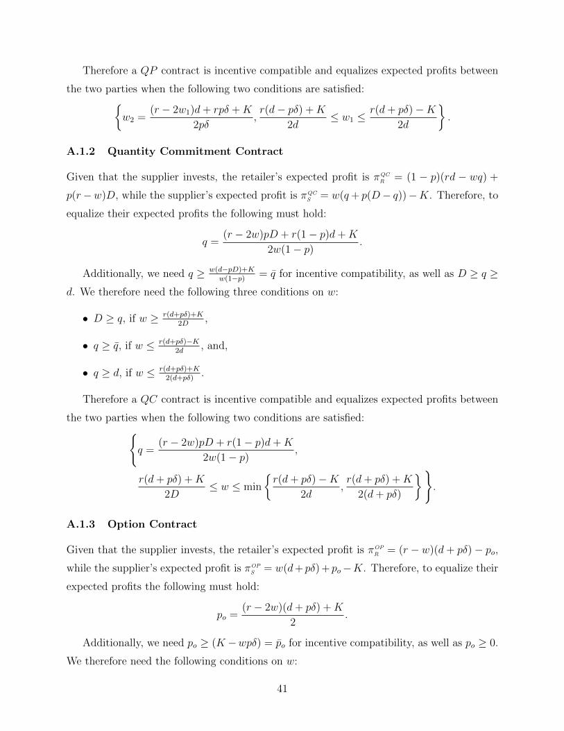
Therefore a QP contract is incentive compatible and equalizes expected profits between

the two parties when the following two conditions are satisfied:{w2 =

(r − 2w1)d+ rpδ +K

2pδ,r(d− pδ) +K

2d≤ w1 ≤

r(d+ pδ)−K2d

}.

A.1.2 Quantity Commitment Contract

Given that the supplier invests, the retailer’s expected profit is πQCR = (1 − p)(rd − wq) +

p(r−w)D, while the supplier’s expected profit is πQCS = w(q+ p(D− q))−K. Therefore, to

equalize their expected profits the following must hold:

q =(r − 2w)pD + r(1− p)d+K

2w(1− p).

Additionally, we need q ≥ w(d−pD)+Kw(1−p) = q for incentive compatibility, as well as D ≥ q ≥

d. We therefore need the following three conditions on w:

• D ≥ q, if w ≥ r(d+pδ)+K2D

,

• q ≥ q, if w ≤ r(d+pδ)−K2d

, and,

• q ≥ d, if w ≤ r(d+pδ)+K2(d+pδ)

.

Therefore a QC contract is incentive compatible and equalizes expected profits between

the two parties when the following two conditions are satisfied:{q =

(r − 2w)pD + r(1− p)d+K

2w(1− p),

r(d+ pδ) +K

2D≤ w ≤ min

{r(d+ pδ)−K

2d,r(d+ pδ) +K

2(d+ pδ)

}}.

A.1.3 Option Contract

Given that the supplier invests, the retailer’s expected profit is πOPR = (r − w)(d+ pδ)− po,

while the supplier’s expected profit is πOPS = w(d+ pδ) + po−K. Therefore, to equalize their

expected profits the following must hold:

po =(r − 2w)(d+ pδ) +K

2.

Additionally, we need po ≥ (K −wpδ) = po for incentive compatibility, as well as po ≥ 0.

We therefore need the following conditions on w:

41

• po ≥ po, if w ≤ r(d+pδ)−K2d

, and,

• po ≥ 0, if w ≤ r(d+pδ)+K2(d+pδ)

.

Therefore, an OP contract is incentive compatible and equalizes expected profits between

the two parties when the following two conditions are satisfied:{po =

(r − 2w)(d+ pδ) +K

2, w ≤ min

{r(d+ pδ)−K

2d,r(d+ pδ) +K

2(d+ pδ)

}}.

A.2 Renegotiation-Proofness of Contracts

While not a primary focus of our research, in evaluating the efficacy of contracts as a solu-

tion to the problem of ex ante investment the literature has often considered whether the

contracts can survive potential renegotiation ex post (see Noldeke & Schmidt (1995) for an

experimental analysis). We briefly discuss here the potential robustness to renegotiation

of the contracts we consider. Note that this is a theoretical analysis, as our experiment

did not allow for the possibility of renegotiation. In our setting there is no scope for a

Pareto-improving offer of renegotiation. Instead, the retailer can only threaten to order an

inefficient quantity. As Lyon & Rasmusen (2004) demonstrate, when renegotiations involve

threats to take inefficient actions, the form of the renegotiation process can significantly

affect the scope for renegotiation and therefore the restrictiveness of requiring contracts to

be renegotiation-proof. We consider here a simple and plausible renegotiation game. Since

we are concerned with potential threats to the supplier’s incentive to invest, we will focus

on the retailer attempting to renegotiate and capture more of the surplus.

After the retailer and supplier agree to a contract and demand is realized, the retailer

can attempt to renegotiate the terms of the contract and increase his profit. Specifically, we

assume that the retailer can credibly threaten to purchase less than the optimal quantity

- down to a minimum of zero units (or the minimum quantity in the case of the Quantity

Commitment contract). The retailer can further offer to order to correct amount if the

supplier agrees to changing the terms of the contract in the retailer’s favor (e.g. by lowering

the wholesale price). We assume that this is a “take it or leave it” offer in order to maximize

the retailer’s ability to renegotiate (and hence make renegotiation-proofness a potentially

substantial restriction). Under the Wholesale Price and Quantity Premium contracts, the

retailer’s threat would give the supplier zero profit from the trade, and therefore (based on

42

the usual results for ultimatum bargaining with standard preferences) the supplier would be

willing to accept any renegotiation offer that gives him at least zero transaction profit (e.g.

setting the wholesale price to zero). Note that the investment cost is sunk, and so does not

affect the renegotiation. It is clear how the prospect of future renegotiation undermines the

suppliers willingness to invest in capacity. If he knows that ex post his revenue from trading

will be driven to zero, then the supplier will prefer not to invest.

The Quantity Commitment, Option and Service Level contracts each change the rene-

gotiation dynamic by ensuring the supplier a minimum profit from the transaction that

cannot be eliminated by the retailer’s threats. In the case of the Quantity Commitment

contract, the contract ensures a minimum order and therefore restricts the scope of the re-

tailer’s threat. For the Option and Service Level contracts the option fee po is paid to the

supplier independent of how many units are purchased, and hence the value of the option

fee cannot be reduced by the retailers threat. Hence if the minimum quantity or option fee

is set sufficiently high investment will be incentive compatible even if renegotiation were to

occur. We detail below conditions for each of these contracts to be renegotiation-proof.

A.2.1 Quantity Commitment

The minimum order q is contractually enforceable, as long as the supplier has sufficient

capacity to deliver the required units (i.e. as long as he invests). Therefore, if the supplier

invests the retailer can at worst threaten to only order q units. If the supplier cannot supply

the required units, the minimum quantity commitment is voided and the retailer is free

to threaten to order zero units27 Hence, for an initial contract (w, q) under any demand

realization the retailer’s renegotiation will yield the supplier a profit of wq − K if he has

invested, and 0 if he has not. The supplier’s incentive compatibility condition is therefore:

q ≥ K

w

Note that for our experimental parameters, if w = 5 the requirement is that q ≥ 7 - hence

any q is sufficient.

A.2.2 Option

If the supplier invests, under the contract he will receive po from the initial option fee. The

retailer will then threaten to order zero units, and will therefore renegotiate away any of

27Similar arguments can show that the QC contract can be written to be renegotiation-proof under thealternate assumption that a failure to invest in capacity only releases the retailer to order down to d units.

43

the retailer’s profit from the sale of the units. If the supplier does not invest he forfeits the

option fee po, and the retailer still renegotiates away any transaction profits. Hence, for an

initial contract (w, po) under any demand realization the retailer’s renegotiation will yield

the supplier a profit of po−K if he has invested, and 0 if he has not. The supplier’s incentive

compatibility condition is therefore:

po ≥ K

Note that for our experimental parameters, the retailer’s individual rationality contraints

are po ≤ 150 (for the base parameters) and po ≤ 250 (for the alternative parameters)

A.2.3 Service Level Agreements

Service Level contracts operate under renegotiation similarly to option contracts - with the

exception that the supplier retains the initial fee po even if he does not invest if demand

is low. Therefore, for an initial contract (w, po) the retailer’s renegotiation will yield the

supplier an expected profit of po − K if he has invested, and (1 − p)po if he has not. The

supplier’s incentive compatibility condition is therefore:

po ≥ K/p

The individual rationality requirements are the same as for the OPT contract.

We can summarize our results as follows:

Proposition 1 There exists incentive compatible and renegotiation-proof OP , SLA and QC

contracts.

A.2.4 Observed Contracts

We did not allow for renegotiation in our experiment - and the prospect of renegotiation

would likely have changed the contractual terms. However, we note that we observe contracts

that would have been renegotiation-proof (under the mechanism we consider) in all three

contracting settings. For Quantity Commitment 91% of contracts in the main treatment

(99% of contracts under the alternate parameters) would satisfy the renegotiation proof-

ness criterion. Similarly, 20% (23%) of Option contracts, and 2% (2%) of Service Level

Agreements. Hence we might anticipate that possibility of renegotiation would to much

larger changes in the observed contracts for OP and SLA than for QC contracts.

44

A.3 IC Region for Superficially Fair Contracts

We now consider the size of the Incentive Compatible regions within our model for OP ,

SLA and QC contracts that are superficially fair (i.e. where w = r/2). We maintain the

underlying structure of the model (e.g. bi-valued demand, binary investment decision, etc.),

but consider variations in the parameters of the model (d,D, r, p,K). For the investment

problem to be non-trivial, we maintain throughout that K < rpδ < 2K (so for example a

superficially fair wholesale price contract will not be incentive compatible on its own). We

begin by reformulating the IC and IR constraints to separate out the common factors across

contracts, given that w = r/2.

For the OP contract, the IC constraint is po ≥ K − pwδ, or 2po ≥ 2K − rpδ. Define

Θ = 2K − rpδ, which represents the additional incentives that the secondary term in the

contract must provide, given the incentives that the wholesale price is already generating.

Note that 0 < Θ < K. The IC constraint is therefore po ≥ Θ/2. The retailer’s expected

profit given the contract (and investment) is

(1− p)(r − w)d+ p(r − w)D − po = (r/2)(d+ pδ)− po

Define Γ = (r/2)(d+ pδ), which denotes the retailer’s remaining surplus given the wholesale

price. Note that Γ > Θ. The IR constraint is therefore po ≤ Γ. The size of the incentive

compatible region for the OP contract is therefore 1−Θ/2Γ. Finally, since Γ > Θ, the size

of the IC region is at least 50%.

For the SLA contract, by similar logic the IC constraint is po ≥ Θ/2p and the IR

constraint is po ≤ Γ. Therefore the size of the IC region is 1 − Θ/2pΓ, which is strictly

smaller than the OP region.

For the QC contract, we can rewrite the IC constraint as pwδ + (1− p)w(q − d) ≥ K or

(1− p)r(q − d) ≥ Θ. Finally, we can write the IC constraint as (q − d) ≥ Θ/r(1− p). Note

that 0 ≤ (q − d) ≤ δ. For the IR constraint we can write the retailer’s expected profit as

(1− p)(r − w)d+ p(r − w)D − (1− p)w(q − d) = Γ− (1− p)w(q − d)

The IR constraint is therefore (q−d) ≤ 2Γ/r(1−p). Note that there are two cases. In Case 1,

this limit is larger than δ, hence the IR constraint will not bind. In Case 2, 2Γ/r(1− p) < δ,

which occurs if d < (1 − 2p)δ. In Case 1 the size of the IC region of the QC contract is

1−Θ/rδ(1− p), while in Case 2 it is 1−Θ/2Γ.

45

Is it possible for the IC region for the QC contract to be larger than the OP contract?

We take the two cases in turn. For Case 1, we want to see if 1 − Θ/rδ(1 − p) > 1 − Θ/2Γ.

This would occur if 2Γ < rδ(1− p), or d < (1− 2p)δ - however this violates the assumption

that we are in Case 1. Therefore, for Case 1 OP always has a larger IC region than QC.

For Case 2, both contracts have the same size region: 1 − Θ/2Γ. Therefore, the size of the

IC region for the OP is always at least weakly larger than the size of the IC region for the

QC contract.

For the QP contract, we know that we at least need w2 > r/2 (since we have assumed

that the problem is not trivially solved by a superficially fair wholesale price contract).

Since w2 ∈ [0, r] is the individually rational region, the IC region is no larger than 50% of

the contracting space. Therefore, the OP contract always has a strictly larger IC region

than the QP contract.

We can summarize our results as follows:

Proposition 2 For superficially fair contracts (w = r/2), the OP contract has an incentive

compatible region that is strictly larger than the region for QP and SLA contracts, and is

weakly larger than the region for QC contracts.

A.4 Example Bargaining Screen

46

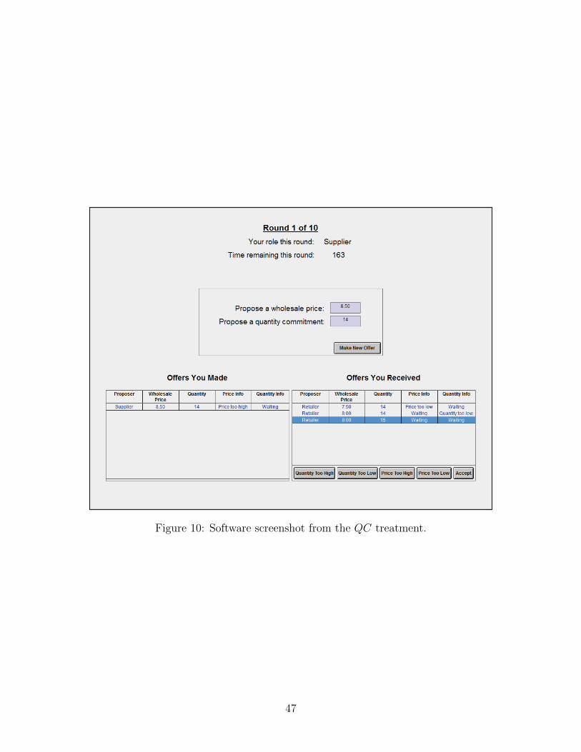
Figure 10: Software screenshot from the QC treatment.

47

contracts and capacity investment in supply chains and capacity investment in supply chains andrew...

Documents