Contract Incompleteness, Contractual Enforcementand Bureaucracies1

Galina A. Schwartz

This paper explains a frequent coexistence of deficient property rights and heavy

bureaucracies. We suggest that in environments with insecure ownership bureaucracies

substitute for enforceable contracts. We study irreversible investment in an asset, and

model the property allocation as a game between a ruler and investors. Since the ex

ante ownership allocation is not enforceable, an ex post share increase is optimal for

the ruler. His share adjustment is costly; the heavier the bureaucratic machine the

higher his cost. Bureaucracy improves investment incentives by reducing the wedge

between the ruler’s ex ante and ex post equilibrium shares.

Economics as a separate science is unrealistic, and mislead-ing if taken as a guide in practice. It is one element – avery important element, it is true – in a wider study, thescience of power.

Bertrand Russell

Introduction

Environments with incomplete or non-enforceable contracts distort property

rights and result in underinvestment. The problem of underinvestment orig-

inates in the divergence of ex ante and ex post incentives to invest. In the

absence of enforcement mechanisms, any ex ante contract is obsolete ex post,

when investment is sunk. Such contracts are routinely renegotiated and the

resulting investment level is lower than when contracts are enforceable. To im-

prove investment incentives, economic agents employ a variety of commitment

mechanisms to induce honoring of the ex ante contract. The reputation-based

mechanisms have been studied most extensively.1I thank Avinash Dixit for turning my attention to this topic, Ariel Rubinstein and Dilip

Abreu for encouragement, Alessandro Lizzeri and Timothy van Zandt for discussions, PatrickBolton for detailed suggestions and practical connections, and, importantly, Faruk Gul forguidance and advice. I am indebted to Prita Subramanian, Carrie Thompson and MikeSchwarz for corrections and to my son for his stoicism in the neglect associated with myPh. D. completion. Financial support from the Ford Foundation is gratefully acknowledged.The remaining errors are mine.

1

This paper suggests that in environments with insecure property rights the

bureaucratic machine is another important commitment mechanism.2 We argue

that in such cases bureaucracies serve a specific role and act as a substitute

for enforceable contracts.3 We suggest that bureaucratic machinery introduces

additional rigidities in ex post contract renegotiation and through that, curtails

disincentives to invest caused by contract non-enforceability.

The proposed commitment mechanism addresses a particular question of

investment inefficiency in cases where a contractual solution is infeasible. How-

ever, the mechanism can be viewed as a generic tool for modelling the principal-

agent problem. Any situation formalized as a resource allocation where ex ante

allocation is altered ex post at a cost, embeds a commitment conflict and could

be modelled with the setup proposed below.

We study irreversible investment in an asset over which the property rights

are unclear. We model the allocation of property rights as a game between a

ruler and investors. Player ownership shares are determined by their relative

bargaining powers, which the ruler could alter at some cost by using the bureau-

cratic machinery. The term ruler refers to any political arrangement ranging

from a feudal lord in Medieval Europe to a head of government, city mayor or

other elected or appointed authority.

First, the players sign an ex ante contract. The allocation of ownership rights

specified by this contract is not enforceable. Then, the investors choose the

investments according to their expectations of the ex post ownership allocation.2The lengthy technology slowdown subsequent to the fall of the Roman Empire is ex-

plained by economic historians by the decay of state provisions, such as infrastructure andlegal framework. McNeil [1986] in “History of Western Civilization” provides the followingdescription of the collapse of the Roman Empire. “The landowners who had staffed the im-perial bureaucracy, commanded the Roman armies, and dominated provincial municipalitieswere crushed down by the weight of taxation. ... Money taxes became steadily more difficultto collect; and levies in kind, extracted in accordance with no sort of law, came to form theprincipal support of the army and of the state. Tax collection amounted to a little more thanorganized robbery... The Senatorial Class of the second century was largely destroyed; andwith it perished the civilian, constitutional, peculiarly Roman, conception of government.”

3The analysis of other bureaucratic functions is beyond the scope of this paper.

2

After the investment is sunk, in the ex post subgame the ruler can modify the

ex ante property rights allocation at the exogenous cost of compensating the

bureaucracy for his ownership share increase. The marginal cost of his share

adjustment increases with the magnitude of adjustment, reflecting the usual

assumption of decreasing returns in production. Bureaucracy is passive and does

not behave strategically to extract part of the surplus.4 Wilson [1989] suggests

that one of the reasons for bureaucratic rigidity relates to the organizational

culture, which permits to minimize the conflict and simplify the management.

Derthick [1990] considers how the Social Security Administration (SSA) coped

with the tasks to administer Supplemental Security Income (SSI) and Disability

Insurance (DI).

The administration of SSI requires the SSA to decide who is needy and of DI

– who is disabled. Both tasks are in conflict with the initial SSA ‘philosophy’

and task to administer the retirement benefits, which went to everybody who

paid taxes into Social Security and who reached a certain age. These new tasks

were fundamentally different from the initial SSA ‘philosophy’ of Social Secu-

rity (by which was meant the commitment to serving beneficiaries). Derthick

showed that efforts to cope with these tasks nearly overwhelmed the agency.

SSA experienced a managerial nightmare and it “suffered an incalculable loss

of prestige, morale, and self-confidence.” [Derthick [1990]]

Massive bureaucracy reduces the ruler’s incentives to increase his ownership

share thereby improving investment incentives. We prove that there exists an

equilibrium of the above presented game. The ruler’s equilibrium payment to

bureaucracy increases when player surplus and the asset value increase. When

the game has multiple equilibria, the Pareto-dominant equilibrium has the high-

est payment to bureaucracy and the lowest ruler’s ownership share.4See Wilson [1989] on low incentives in bureaucracies and their tendency to be rigid and

reluctant to change, and Dixit [1997] for the game-theoretic analysis.

3

Empirical evidence [Clarkson [1996]] suggests that contracts between state

and local authorities, determining state versus local taxes are incomplete. He

argues that contract incompleteness is a result of the inability of both state and

city authorities to commit to their ex ante tax rate promises. His finding sup-

ports the observation from the regulation literature that there is a commitment

problem for government authorities and public institutions even in countries

with a well-developed legal framework.

The literature on contract law and its enforcement in different economic en-

vironments can be classified into three groups. The first group, belonging to

industrial organization, investigates the impact of a regulatory regime on invest-

ment and analyzes public goods provision.5 The second relates to international

economics; it considers honoring international trade treaties and other govern-

ment obligations.6 The third group consists of economic history papers that

examine contract enforcement in the absence of a legal system.7

The most comprehensive treatment of the subject is provided by the regu-

lation literature. 8 The Coase [1960] theorem asserts that an optimal resource

allocation is achievable through market forces, irrespective of the legal liability

assignment, if information is perfect and transactions are costless. When the

assumption of perfect information does not apply, or when transaction costs are

present, government intervention may be desirable. The subject was studied in

industrial organization literature and relates to the question of how to provide

the efficient amount of specific investment.9

Consider the allocation of property rights for an asset produced by a regu-5Public goods provision is closely related to regulation, see Shapiro and Willig [1990] for

a series of ‘neutrality results’, that is, identification of informational environments with nointrinsic difference in the performance of public and regulated private enterprise.

6Reviewed by Staiger [1995].7Reviewed by Grief [1996].8Reviewed by Noll [1989].9Laffont and Tirole’s [1994] book is an encyclopedic reference on the subject.

4

lated firm. The firm’s ownership rights over the asset are limited and dependent

on the regulatory restrictions. The ex ante property rights allocation resulting

from these restrictions is frequently suboptimal ex post, and it is optimal to alter

it ex post for social efficiency. This causes an ex post commitment problem for

the regulator and results in investment distortion. The literature bearing on the

principal-agent problem is far too extensive for reviewing, or even listing it here.

Tirole (1999) provides a comprehensive outlook of the incomplete contracting

literature.10

Anderlini and Felli [1997] study property rights by using bargaining games.

They consider a hold up problem in the presence of ex ante contract costs and

investigate the conditions under which socially efficient contracts are infeasible.

In their initial setup, the distribution of bargaining power across agents is ex-

ogenous, and the resulting contracts are constrained inefficient. The inefficiency

arises for a certain range of the bargaining powers of the players. Further, An-

derlini and Felli [1997] endogenize the distribution of the surplus across players.

For a certain range of ex ante contract costs, socially desirable contracts are

not feasible, irrespective of the surplus distribution. Anderlini and Felli [1997]

suggest that when the potential surplus depends on its distribution, the hold

up problem is less acute.

Our model is analogous to the Anderlini and Felli [1997] setup when the

potential surplus is dependent on its distribution. While in their paper only two-

party games are considered, we consider multi-party contracts, and our model

permits multi-period contacts. Their model is applicable to a wider range of

environments, while our focus is the mechanism behind the surplus distribution.

Greif [1996] points out that historically exchange and contract enforcement

existed even in the absence of a legal system. The examination of this phe-10For recent developments see Review of Economic Studies, (1999), Vol. 66, Issue 226.

5

nomenon has not advanced due to the lack of an appropriate framework. How-

ever, the existing studies indicate that it is misleading to view contract enforce-

ment based on formal organizations and repeated interactions as substitutes

[Greif [1996]]. The intuition for this argument parallels the intuition for why

equilibria supported by reputation are typically Pareto inefficient. While in

some cases efficiency can be reach through informal means, in both perspectives,

historical and theoretical, resource allocations that rely on the rule of law are

welfare superior to the ones that rely on informal agreements. The enforcement

based on informal interactions relates to formal enforcement as pre-monetary

systems of exchange to a monetary system with sophisticated banking institu-

tions.

Our model provides further support for this argument. We show that quasi

property rights that rely on the bureaucratic machinery rather than on enforce-

able contracts are an imperfect substitute for enforceable contracts and real

property rights. Davies [1977] provides an example of inefficiency associated

with the public provision. He compares the state-owned Trans Australian Air-

lines (TAA) with the privately-owned Ansett Australian Airlines. Despite the

fact that both are tightly regulated by the government, charge the same fares,

pay essentially the same wages, and are allowed to compete only with respect

to minor amenities, Ansett is more efficient (that is, uses fewer employees to

transport a given amount of freight or number of passengers) than TAA. Davies

suggests that the difference between the TAA and Ansett relates to the differ-

ence in the property rights structure.

The paper is organized as follows: in Section I, the model is presented as an

extensive form game. In Section II, the equilibria of the game are characterized

and welfare implications analyzed. In Section III, the limitations and extensions

of the model are considered, followed by a concluding remark. To ease the

6

exposition technical details and proofs are relegated to the Appendices.

I. The Model

Initially property rights for an asset are unclear. They emerge in the game

Γ between a ruler and N identical investors. The game has three stages. In

the first stage, the players sign a non-enforceable ex ante contract.11 In the

second stage, investors simultaneously make their irreversible investments in

the asset, which value is increasing and concave in total investment, or invest

in the outside option with a fixed investment return denoted by i. In the third

stage, the ex ante contract is revised, an ex post contract is drawn, and the

asset is divided between the players, in accordance with the ex post contract.

The significance of the ex ante contract is its effects on the ex post contract.

The ruler possesses some control over the asset, but does not have complete

property rights over it. He cannot sell the asset or invest in it, and lacks the

right or expertise to use it for production. Thus, to benefit from controlling the

asset, the ruler has to contract with the investors. Examples of such assets are

numerous: an oil field, a municipal building or agricultural land.12 To adjust

his ownership share the ruler uses bureaucracy. Drastic share adjustments are

relatively more costly than minor ones.

Bureaucracy is a government or private institution capable of altering the

current division of the surplus between the players. There are many mechanisms

to channel the bureaucratic provisions into bargaining powers and through that

affect the ownership allocation13. We suggest that bureaucratic red tape affects11An absence of enforceability is a stronger constraint on applications than is actually

needed. Let investment in the asset be partially contractible, with the effects of contractibleand non-contractible investments on its value being independent. Then, one can consider thenon-contractible component as a separate asset.

12The asset may be interpreted as GNP, investment as aggregate investment, and the ruleras the head of the government. Then, his ownership share is a tax rate, explicit or implicit.

13Bureaucratic provisions are laws, decrees, directives, or any other rules relevant for deter-mination of the bargaining balance.

7

the relative speed of player responses. In many situations, red tape could be

circumvented by bribes, which indicates its relevance for surplus redistribution.

Red tape is a routine bureaucratic instrument for altering the reaction time,

and thus, the distribution of the surplus. Thus, bureaucracy is a device, or a

mechanism which affects property right allocation.

In the ex ante stage, the ruler chooses his ownership share without incurring

any cost. In the ex post stage, the ruler can change his ownership share at an

exogenous cost. This cost is equal to the expense that bureaucracy incurs to

institute the change. Property rights for the asset are allocated according to

the outcome of the ex post game.

To summarize, the game Γ is the game of complete information. The game

has N + 1 players, the ruler and N investors, and the following order of moves.

First, the ruler chooses his ex ante share x ∈ [0, 1]. Then, the investors choose

their investments qN ∈ [0,∞). The total investment Q =∑N

n=1 qN determines

the asset value P (Q). Third, the ruler chooses his ex post share y ∈ [0, 1].

Each investor’s objective is to maximize his profit, ΠN(x, y,q), and the ruler’s

objective is to maximize his net surplus, V (x, y,q). The n-th investor’s profit

is equal to the value of his ex post ownership share less his opportunity cost

to funds iqN , and the ruler’s net surplus is equal to the value of his ex post

ownership share net of his adjustment cost B(y − x):

Πn(x, y,q) = qn

Q (1− y)P (Q)− iqn,

V (x, y,q) = yP (Q)−B(y − x),(1)

where n = 1, ..., N and q = (q1, ..., qN ) is the vector of investments. The asset

value is continuous, concave and three times continuously differentiable at any

Q ∈ (0,∞). In the absence of property rights conflict investment in the asset

is positive, i.e. the derivative of the asset value evaluated at zero exceeds the

8

outside option return P ′(Q):

P ′(Q) > 0, P ′′(Q) < 0, limQ→0

P ′(Q) →∞.(2)

The function B(z) is continuous, convex, three times continuously differentiable

for any z ∈ (0, 1):

B′(z) > 0, B′′(z) > 0.

and can be discontinuous at zero, reflecting the possibility of a fixed-cost.

The equilibrium concept used to analyze this game is a subgame perfect

Nash equilibrium that are symmetric with respect to the investors. In such

equilibria, investor actions are identical and, since the ruler’s objective depends

on aggregate investment (not on individual investments), it is sufficient for him

to condition his actions on aggregate investment.

II. The Equilibrium of the Game

We say that an investment market is monopolistic if investment in the asset

is done by one investor only. If the number of investors is finite, an investment

market is imperfectly competitive. A perfect competitive investment market is

the limiting case of infinitely many investors.

Definition 1. An equilibrium is dynamic if the ruler’s ex ante and ex post

actions differ (x 6= y), and static if they are the same (x = y).

Assume the ruler can commit to the ex ante contract. Let Γ denote the game

that the committed ruler plays. Its Pareto-dominant outcome will be called the

commitment outcome.

Theorem 1. An equilibrium of the game Γ exists and the ruler’s payoff is

strictly positive.

9

Proof: See Appendix. �

The intuition for the proof is summarized below. The proof is by backward

induction. From the ruler’s ex post first order conditions, he has at most two

ex post best responses, one in which he adjusts his ownership share, and one

in which he does not. Moreover, along the equilibrium path, his ex post best

response is unique.

Substitution of the ruler’s ex post best response in investor objective function

permits us to solve the investors’ maximization problem. There exists one ex

ante share for which investor best response is not unique, but we prove the

uniqueness of an equilibrium that could originate at this share. Therefore, on

the equilibrium path, an equilibrium of the subgame that starts at a specific

ruler’s ex ante share is unique.

The last step is to find the ruler’s optimal ex ante action by using the ruler’s

ex post best response and investor best response. The ruler has at most a finite

number of optimal ex ante actions, and the game has at most a finite number

of equilibria.

Figures I – III provide investor best responses to the ruler’s adjustment

cost function B(z) with different properties. Figure 1 assumes a non-zero

fixed cost ( limz→0

B(z) > 0), and Figures II and III – a zero ruler’s fixed cost

( limz→0

B(z) = 0) and, respectively, the discontinuous ( limz→0

B′(z) > 0) and contin-

uous ( limz→0

B′(z) = 0) first derivative of the function B(z) at zero.

Remark 1. Without bureaucracy, the ruler’s ex post incentive is to expropriate

the whole asset, which results in zero surplus for all the players.

Notice, that the ruler’s equilibrium payoff is always strictly positive, because

investor best response to any ex ante share other than x = 1 is strictly positive.

When the investment market is imperfectly competitive, investor profit is also

always strictly positive. Therefore, from Remark 1 and Theorem 1, the presence

10

of bureaucracy improves player surplus and positively affects society’s welfare.14

Theorem 2. There exists a Pareto-dominant equilibrium in the game Γ. The

asset value in the Pareto-dominant equilibrium is the highest and the rule’s

ownership share — the lowest within the set of the respective equilibrium values

in the game Γ.

Proof: See Appendix. �

When the game Γ has several equilibria, the ruler’s welfare is the same

across equilibria, because he moves first and his ex ante action determines which

equilibrium occurs. In the case of multiplicity of equilibria, investor welfare is

the highest in the equilibrium with the highest asset value. This equilibrium

is dynamic and has the lowest ruler’s ownership shares, ex ante and ex post.

The equilibrium with the highest asset value is Pareto-dominant despite the

fact that the dissipation of the surplus on bureaucratic costs is the greatest.

Thus, an equilibrium with a positive payment to bureaucracy is always Pareto

superior to the equilibrium in which the bureaucratic presence is latent. When

the equilibrium of the game is dynamic, bureaucratic costs are positive, and

player commitment payoffs are not achievable. Nevertheless, the players’ welfare

increases with the bureaucratic machinery.

The usual perception is that bureaucracy guards the ruler’s interests. In

our model, bureaucracy is really the ruler’s tool and safeguard, used to secure

a higher payoff for the ruler’s than he would have had otherwise. Interestingly,

from Remark 1 bureaucratic presence also benefits the investors. With bu-

reaucracy, aggregate equilibrium profit of imperfectly competitive investors is

strictly positive, while it is zero otherwise. Bureaucracy imposes a cost on the

ruler and through that constrains his ability to expropriate surplus. Bureau-14Society’s welfare could be defined as the game surplus. Alternatively, adjustment cost

could be included in society’s welfare.

11

cracy improves investor payoffs since the bureaucratic machinery is a constraint

on all players.

Theorem 3. In an equilibrium of the game Γ the asset value and each player

payoff are bounded by the respective commitment outcome values. Player sur-

plus reaches the commitment surplus only if the commitment outcome is an

equilibrium of the game Γ.

Proof: See Appendix. �

This result that the equilibrium asset value never exceeds the commitment

asset value is intuitive. When commitment outcome is not sustainable, bu-

reaucracy constrains the ruler from expropriating the entire asset, but this con-

straint is insufficient to eliminate the commitment problem completely. Thus,

the equilibrium asset value is between the optimal value and zero, which would

have been an equilibrium asset value in the absence of the bureaucracy. To ease

the comparative analysis of the games differing by the number of investors, we

assume P ′′′ < 0.

Theorem 4. In the equilibrium of the game Γ, the asset value and the ruler’s

payoff increase in the number of investors.15

Proof: See Appendix. �

It follows from Theorem 1 that the equilibrium is dynamic if the asset value

exceeds a critical value. By Theorem 4 if the number of investors increases,

the asset value also increases. Hence, the equilibrium might switch from a

static to a dynamic one as the number of investors increases. In this case, the

bureaucracy starts receiving a positive payment from the ruler, but total player

surplus is higher than when the equilibrium is static. Figure IV illustrates how

the equilibrium of the game Γ depends on the number of investors.15We can prove Theorem 4 without restriction on the third derivative of the function P .

12

III. Discussion and Conclusion

1. Connection to Contract Theory

Models, which address the hold up problem, investigate the divergence of

the ex ante and ex post incentives to invest. These models propose instruments

or mechanisms to lessen or eliminate this divergence. Whether it is possible to

find a contractual solution depends on the nature of the divergence and on the

proposed mechanism. Hart and Moore [1988] argue that nonverifiability implies

noncommitment. In this spirit, our model could be used to study incomplete

contracts. Formally, many cases of nonverifiability are indistinguishable from

noncommitment.

In this paper, we are studying the problem of underinvestment in environ-

ments with unclear property rights. We presented the game Γ as a tool for

analyzing this problem. However, the game Γ provides a basic setup for general

modeling of environments with limited commitment or costly contracts. Any

situation which can be formalized as a resource allocation problem, with ex

ante allocation that could be altered ex post at a cost, convex in the altered

parameter, can be modeled with the proposed setup.

Even when contracts are enforceable, renegotiations frequently occur. The

model can be adopted to study optimal renegotiation structure, and design op-

timal penalties for breaking the terms of the contract. The cost of bureaucracy

could be interpreted as a penalty imposed on a defaulting party. Specific func-

tional forms reflecting characteristics of a particular environment can be used

to design more efficient contractual and legal procedures, with the adjustment

cost function viewed as a legal or penalty cost.

2. Extensions and Applications

2A. Strategic Bureaucracy: Our model does not account for strategic

13

bureaucracy, but suggests several modifications for modelling it. The net effect

of strategic bureaucracy on the investment allocation is not clear-cut. On one

hand, strategic bureaucracy is welfare improving, as it imposes an additional

constraint on the ruler and lessens his commitment problem. On the other hand,

with strategic bureaucracy, investor ownership share of the asset may be lower

due to the ruler’s higher ex ante share.

2B. Investor Influence on the Ownership Allocation: Our model

in its current form does not allow the investors to directly affect the property

rights allocation. The investors’ only influence on ownership rights is indirect:

through their investment choices.

There are several ways to overcome this limitation. One way is to modify the

game and allow all players to pay the bureaucracy for a favorable adjustment of

their ex post ownership shares. Such game is considered in Schwartz (2003) and

used to explain a proliferation of the Preferential Trade Areas. An alternative

way is to allow the ruler to invest in the asset ex ante.

3. Economic Policy and Insecurity of Property Rights

3A. Deregulation and Privatization: An easy reform, especially when

the legal system is weak, can be dismantled by the next not necessarily benev-

olent ruler. We suggest, that a typical complication of economic reforms by

bureaucratic resistance to change reflects the role of bureaucracy as a substitute

for enforceable contracts.16 From this angle, bureaucratic resistance to reform

appears to be a necessary evil that should be exploited rather than fought. In

such an environment it is not plausible to model bureaucracy as passive as it is

more likely to play a strategic role.

The investment distortion is more substantial if the investment markets are

less competitive. Therefore, monopolistic publicly owned enterprises or regu-16See, for example, a discussion of Russian economic reform in Sachs and Pistor [1997].

14

lated industries are the most distorted. Paradoxically, monopolistic markets are

exactly where regulation is most active.

Hence, deregulation or privatization in industries with less competitive in-

vestment markets generates a Pareto improvement that is impossible to mimic

even through complete commitment of regulatory authority to a declared regime.

This intuition is supported by the current trend of deregulation and denation-

alization.17

3B. Restrictions on Domestic Investment Market: Restricted ac-

cess to investment markets is frequently observed in environments with insecure

property rights. Two types of such restrictions occur. First, the investors might

be prohibited from investing abroad or, more generally, capital mobility may

be restricted. Second, investor access to certain markets could be restricted.

Typically, both types of restrictions are observed simultaneously: when foreign

investment is restricted, domestic investors are also subject to the limitations

of investment market competitiveness.

The first type of restriction improves the ruler payoff through a lower outside

return. The second type of restrictions, i.e., the limitations of investment market

competitiveness, is harder to explain. We suggest that such restrictions are likely

to occur in repeated settings, when the equilibrium favors investors.

4. Concluding Remark

The beneficial effect of a bureaucratic presence on the investment climate is

not at all intuitive. The intellectual resistance to positive outlook on bureaucra-

cies is understandable. Noted for low incentives and inefficiencies, bureaucracies

are commonly perceived to be a curse rather than a blessing.

We provide a theoretical argument that explains the persistent correlation of

massive bureaucracies and unclear property rights. One could view bureaucratic17See, Joskow and Noll [1994] for an overview of US regulatory reform.

15

constraints on the ruler’s ex post share adjustment as a primitive form of division

of power between the ruler and the bureaucrats that would gradually be replaced

by the rule of law. This paper focuses exactly on this aspect of bureaucratic

rule. The model emphasizes that the positive effect of bureaucratic machinery

on welfare is due to its ability to restrict the ruler’s ex post expropriation. From

this perspective, bureaucracy is an investor guardian angel.

16

Technical Appendices

Appendix I: Figures

Figure I

0 1

ruler’s ex ante ownership share x

investor best

response f(x)

f(x) =

q(x) : x ∈ [0, x

¯]

q : x ∈ (x¯, x]

q(x) : x ∈ [x, 1].r

r

rrr rx¯ x

q

f(x)

?

@@

@@R

����9

q(x)�)

q(x)��

Figure I assumes limz→0

B(z) > 0 (and limz→0

B′(z) ≥ 0). Then:

If x ∈ [0, x], best response investment in the game Γ is lower than best response

investment in the game Γ, and if x ∈ [x, 1], best response investments in both

games are the same.

If x∗ ∈ [0, x¯], the equilibrium of the game Γ is dynamic, and If x∗ ∈ [x, 1], the

equilibrium is static. Ex ante shares x ∈ [x¯, x] are never the equilibrium ones.

As the fixed cost decreases, the difference x − x¯

decreases, and reaches zero

(x = x¯) at lim

z→0B′(z) = 0, and Figure I turns into Figure II.

17

Figure II

0 1

ruler’s ex ante ownership share x

investor best

response f(x)

-

6

limz→0

B(z) = 0 and limz→0

B′(z) > 0

r

r

rr

x

f(x)�

��� JJ

JJq(x)�)

Figure II assumes limz→0

B(z) = 0 (and limz→0

B′(z) > 0).

As the derivative limz→0

B′(z) ≥ 0 decreases, the value x¯

= x increases. When the

derivative reaches 0, x¯

= x reaches 1, and Figure II turns into Figure III.

18

Figure III

0 1

ruler’s ex ante ownership share x

investor best

response f(x)

-

6

limz→0

B(z) = 0 and limz→0

B′(z) = 0

r

r

r

f(x)�

� q(x)�

�

Figure III assumes limz→0

B(z) = 0 and limz→0

B′(z) = 0. Then, x¯

= x = 1.

In this case, the game Γ has a unique dynamic equilibrium and the player surplus

is below the commitment outcome surplus (Theorem 3).

19

Figure IV

0 1

ruler’s ex ante (or ex post) ownership share x

investor best

response f(x)

-

6Equilibria of the Games Γ(N1) and Γ(N2)

Let N1 < N2. Then:

q∗N1 < q∗N2. [Theorem 4]

q

q

qss

y∗N2y∗N1

q∗N1

q∗N2

fN1(x)�

��

fN2(x)�

Figure IV assumes limz→0

B(z) = 0 and limz→0

B′(z) = 0, and N1 < N2.

In the equilibrium of the game Γ the asset value and the ruler’s payoff are in-

creasing in the number of investors (Theorem 4).

20

Appendix II: Proofs

Proof of Theorem 1:

The existence of a symmetric equilibrium follows from the construction pre-

sented below. In a symmetric equilibrium, investor actions are identical. Since

the ruler’s objective depends on aggregate investment, it is sufficient for him

to condition the actions on aggregate investment. The proof consists of seven

Steps and is by backward induction. In Step 1 we solve a system of equations.

In Step 2 we solve the game Γ with a restriction for the ruler to employ the

same ex ante and ex post actions. In Step 3 we prove that the solution of the

system of equations introduced in Step 1 provides player best responses for a

certain interval of the ruler’s ex ante shares. In Step 4 we show that for a certain

interval of the ruler’s ex ante actions his ex post best response action is equal

to his ex ante action, and investor best response is equal to their best response

in the restricted game of Step 2. In Steps 4 - 6 we show that there exist x¯

and

x, 0 ≤ x¯≤ x ≤ 1, such that the equilibrium in the subgame that starts after

x ∈ [0, x¯] is dynamic, it is static for all x ∈ [x, 1], and x ∈ (x

¯, x) are never the

equilibrium actions in the game Γ. In Step 7 we establish the uniqueness of the

equilibrium in the subgame that starts after x ∈ [0, x¯] ∪ [x, 1], prove the exis-

tence of an equilibrium and show that the ruler’s equilibrium payoff is strictly

positive.

Step 1: To simplify, we extend functions defined on open intervals to the

closed intervals by continuity. Consider the following system of equations:

P (Q)−B′(y − x) = 0,(3)

(1− y)A(Q)− i = 0,(4)

y > x,(5)

21

where Q ∈ [0,∞), x, y ∈ [0, 1], and A(Q) is equal to

A(Q) =1N

P ′(Q) + (1− 1N

)P (Q)

Q.(6)

From properties of the function P, the function A is continuous and twice con-

tinuously differentiable for all Q ∈ [0,∞) (the function A is a weighted average

of marginal and average costs).

Claim 1. The system of equations (3) - (5) has at most one solution. This solu-

tion (y(x), Q(x)) is continuous, twice continuously differentiable, and Q′(x) < 0.

One can find such an xb ∈ [0, 1] that for all x ∈ [0, xb) a solution of the system

of equations (3) - (5) exists, and for all x ∈ [xb, 1] there is no solution.

Proof of Claim 1: Let b denote limv→0

B′(v) and Qb – the solution of equation

P (Q) = b. For Q < Qb the subsystem of equations (3) and (5) has no solution,

because from properties of the functions B and P for any y > x:

P (Q) ≤ P (Qb) = b < B′(y − x).(7)

Keep Q and x fixed and differentiate equation (3) with respect to y to show

that the derivative is negative:

−B′′(y − x) < 0.(8)

From equation (8) and properties of the functions P and B, there exists a unique

solution of equation (3) for any fixed x and Q ∈ (Qb,∞). Let yQ(x) denote this

solution. Differentiate equation (3) with respect to Q and keep x fixed to show

22

that the derivative dyQ(x)dQ is positive:

dyQ(x)dQ

=P ′(Q)

B′′(yQ(x)− x)> 0.(9)

Use equations (7) and (9) and properties of the functions A, P and B to show

that the derivative of equation (4) with respect to Q is negative:

(1− y)A′(Q)− P ′(Q)B′′(yQ(x)− x)

A(Q) < 0,

because the function A′ is negative

A′(Q) =1N

P ′′(Q) + (1− 1N

)1Q

[P ′(Q)− P (Q)

Q

]< 0.(10)

Thus, there exists a unique interior solution Q(x) of equation (4). (A bound-

ary point Q = 0 is optimal only when x = 1, in which case the system of

equations (3) - (5) has no solution. A boundary point Q → ∞ is never opti-

mal). From uniqueness and existence of yQ(x) and Q(x) there exists a unique

y(x) = yQ(x)(x) and a unique solution (y(x), Q(x)) of the system of equations

(3) - (5) for all x such that Q(x) ∈ (Qb,∞). From the continuity and differ-

entiability of the underlying functions this solution (y(x), Q(x)) is continuous

and twice continuously differentiable. Differentiate equations (3) and (4) with

respect to x and apply the implicit function theorem to show that the derivative

Q′(x) is negative

Q′(x) =i

(1− y)2A′(Q)− iP ′(Q)B′′(y−x)

< 0,(11)

due to properties of the functions A, P and B.

Let xb denote the solution of equation Q(x) = Qb. The system of equations

23

(3) - (5) has no solution for all x ∈ [xb, 1], because from equation (11) Q(x) <

Qb for all x ∈ [xb, 1], and for all x ∈ [0, xb) there exists a unique solution

(y(x), Q(x)). �

Step 2: Let the game Γ denote the game Γ in which the ruler’s ex post

action is restricted to be his ex ante action.

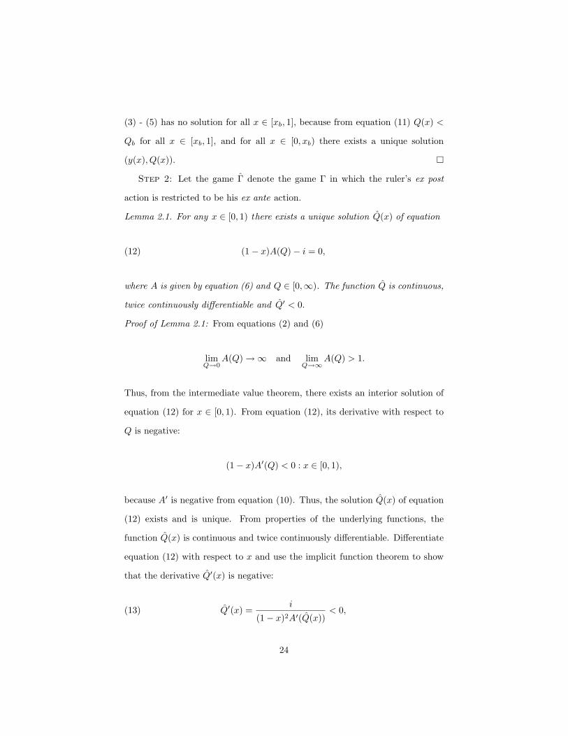
Lemma 2.1. For any x ∈ [0, 1) there exists a unique solution Q(x) of equation

(1− x)A(Q)− i = 0,(12)

where A is given by equation (6) and Q ∈ [0,∞). The function Q is continuous,

twice continuously differentiable and Q′ < 0.

Proof of Lemma 2.1: From equations (2) and (6)

limQ→0

A(Q) →∞ and limQ→∞

A(Q) > 1.

Thus, from the intermediate value theorem, there exists an interior solution of

equation (12) for x ∈ [0, 1). From equation (12), its derivative with respect to

Q is negative:

(1− x)A′(Q) < 0 : x ∈ [0, 1),

because A′ is negative from equation (10). Thus, the solution Q(x) of equation

(12) exists and is unique. From properties of the underlying functions, the

function Q(x) is continuous and twice continuously differentiable. Differentiate

equation (12) with respect to x and use the implicit function theorem to show

that the derivative Q′(x) is negative:

Q′(x) =i

(1− x)2A′(Q(x))< 0,(13)

24

because A′ is negative from equation (10). �

Lemma 2.2. There exists a unique symmetric equilibrium q(x) in subgame of

the game Γ that starts after x, where q(x) = (q(x), . . . , q(x)), q(x) = Q(x)

N ,

and Q(x) is a solution of equation (12). The function q is continuous, twice

continuously differentiable and q′(x) < 0 for all x ∈ [0, 1].

Proof of Lemma 2.2: First, we show that investment q(x) is optimal for each

investor given that all other investor actions are equal to q(x). Second, we prove

that no other vector of investments can be a symmetric investor best response.

1. Let q(x) = ( Q(x)

N , . . . , Q(x)

N ) be the vector of investments. Then, from

Lemma 2.1 each investor’s first order conditions are fulfilled:

Πn(x, x, q(x))dqn

= (1− x)A(Q)− i = 0,

where n = 1, . . . , N . Thus, q(x) is a critical point of the function Πn, because

Πn is concave in qn:

d2Πn(x, x, q(x))dq2

n

= (1− x)A′(Q) < 0,

which provides that each investor profit is maximized at q(x).

2. The proof is by contradiction. Let q(x) = ( Q(x)

N , . . . , Q(x)

N ), with Q(x) 6=

Q(x), be another symmetric investor best response. Then, each investor’s first

order conditions are:

Πn(x, x, q(x))dqn

= (1− x)A(Q)− i = 0,

which contradicts the uniqueness of the solution of equation (12). Thus, the

symmetric best response q(x) is unique. From Lemma 2.1 and equation (13)

the function q is continuous, twice continuously differentiable and decreasing in

25

x:

q′(x) < 0,(14)

for all x ∈ [0, 1]. �

Claim 2. There exists an equilibrium of the game Γ.

Proof of Claim 2: From equation (1) and Lemma 2.2, the ruler’s objective

V (x,q) in the game Γ is to maximize:

V (x,q) = V (x, x,q) = xP (Q(x)),

where Q(x) = N q(x) is aggregate best response investment. The ruler’s payoff

is continuous for all x ∈ [0, 1], is zero at x = 0 and x = 1, and bounded by

[0, Pmax], where Pmax = P (Q(0)). Thus, the ruler’s payoff is continuous and

bounded on the compact interval [0, 1]. Then, a set X of maximizers of the

function V (x,q) is non-empty. From Lemma 2.2 there exists a unique investor

best response for any x, and, thus for all x ∈ X. Therefore, there exists an

equilibrium of the game Γ, with player actions (x, q(x)) and x ∈ X. �

Step 3:

Claim 3. The equilibrium of the subgame that starts after x ∈ [0, xb), in which

the ruler’s ex post best response is greater than x is unique. Player actions in

this equilibrium are (y(x),q(x)), with q(x) = (q(x), . . . , q(x)), q(x) = Q(x)

N and

(y(x), Q(x)) is a solution of the system of equations (3) - (5).

Proof of Claim 3: The ruler’s ex post first order conditions coincide with equa-

tion (3). Its solution yQ(x) provides the ruler’s best response y to any fixed x

and Q, if y > x. From Claim 1 if y > x, there exists a unique ruler’s ex post

26

action yQ(x) > x for any fixed x ∈ [0, 1] and Q ∈ (Qb,∞):

V (x, yQ(x),q) = maxy>x

V (x, y,q),

where Q =∑N

n=i qn. From Claim 1 that there exists a unique solution (y(x), Q(x))

of the system of equations (3) - (5) for all x ∈ [0, xb). From the argument anal-

ogous to Lemma 2.2, if the ex post best response y > x and investor actions are

symmetric maximum profit is achieved at a unique q(x) = (q(x), . . . , q(x)), with

q(x) = Q(x)

N . The function q is continuous, twice continuously differentiable and

q′(x) < 0.(15)

Thus, if the ruler’s ex post best response y is greater than x, a solution (y(x), Q(x))

of the system of equations (3) - (5) provides unique equilibrium aggregate in-

vestment Q(x) and the ruler’s ex post action y(x). �

Step 4: Let G(x) be defined as

G(x) = (y(x)− x)P (Q(x))−B(y(x)− x),

and notice that G(x) equals to the ruler’s maximum gain from the ex post share

adjustment. Let player actions and payoffs indexed by the superscript ‘d’ refer

to the case of a dynamic ruler’s ex post best response, i.e. y > x, and by the

superscript ‘s’ to a static one, i.e. y = x. When G(x) > 0, the ruler’s ex post

best response is dynamic, because his gain from the share adjustment is positive.

Claim 4. If G(x) < 0, the ruler’s ex post best response is static for all x ∈

[0, 1). If

G(x) = 0(16)

27

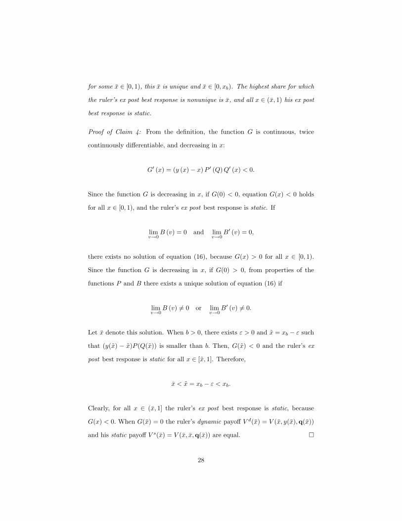
for some x ∈ [0, 1), this x is unique and x ∈ [0, xb). The highest share for which

the ruler’s ex post best response is nonunique is x, and all x ∈ (x, 1) his ex post

best response is static.

Proof of Claim 4: From the definition, the function G is continuous, twice

continuously differentiable, and decreasing in x:

G′ (x) = (y (x)− x) P ′ (Q) Q′ (x) < 0.

Since the function G is decreasing in x, if G(0) < 0, equation G(x) < 0 holds

for all x ∈ [0, 1), and the ruler’s ex post best response is static. If

limv→0

B (v) = 0 and limv→0

B′ (v) = 0,

there exists no solution of equation (16), because G(x) > 0 for all x ∈ [0, 1).

Since the function G is decreasing in x, if G(0) > 0, from properties of the

functions P and B there exists a unique solution of equation (16) if

limv→0

B (v) 6= 0 or limv→0

B′ (v) 6= 0.

Let x denote this solution. When b > 0, there exists ε > 0 and x = xb − ε such

that (y(x) − x)P (Q(x)) is smaller than b. Then, G(x) < 0 and the ruler’s ex

post best response is static for all x ∈ [x, 1]. Therefore,

x < x = xb − ε < xb.

Clearly, for all x ∈ (x, 1] the ruler’s ex post best response is static, because

G(x) < 0. When G(x) = 0 the ruler’s dynamic payoff V d(x) = V (x, y(x),q(x))

and his static payoff V s(x) = V (x, x,q(x)) are equal. �

28

Step 5: Let q denote q(x).

Claim 5. There exists at most one x¯, to which investor best response is nonunique.

When x¯

exists, we have x¯≤ x and:

(1) for x ∈ [0, x¯) ∪ (x, 1] there exists a unique equilibrium in the subgame of the

game Γ that starts after x,

(2) for x ∈ [0, x¯) player best responses are dynamic, and for x ∈ (x, 1] – static,

(3) for x ∈ (x¯, x) investor best responses are q.

Proof of Claim 5: From equations (4), (12), and (14) for all x ∈ [0, xb)

q(x) = q(y(x)) < q(x).(17)

From Claim 4, for x ∈ (x, 1] the ruler’s ex post best response is static, and

x¯≤ x < xb. From Claim 2, investor best response q(x) is unique for all x

¯≤ x.

For x ∈ [0, x) investment q > q cannot be sustained statically, because

G(x) > 0. From Claim 4, for x < x the ruler’s ex post best response to q > q is

dynamic. If x ∈ [0, x) and investment qs < q is sustainable, q is also sustainable

and preferred by the investors to qs. Thus, if x ∈ [0, x) and y = x is optimal for

the ruler, q is optimal for the investors.

Further proof of Claim 5 is by contradiction. Let investor best response to

x1 and x2, x1 < x2, be nonunique:

Π(x1, y(x1),qd1) = Π(x1, x1,qs

1)

Π(x2, y(x2),qd2) = Π(x2, x2,qs

2).(18)

Here qdµ∈{1,2} = (q(xµ), . . . , q(xµ)), and qs

µ∈{1,2} = (q, . . . , q), because xµ ∈

[0, x). From equations (14), (15) and (17) we have

q < q(x2) < q(x1).(19)

29

Use equations (18) and (19) to show that the difference between static and

dynamic profit when the ruler’s ex ante action is equal to x1 is positive:

Π(x1, y(x1),qd1)−Π(x1, x1, q) >

Π(x1, yQ2(x1),qd

2)−Π(x1, x1, q) =

(x2 − x1)[P (N q2(x))− P (N q)] > 0.

(20)

Here Q2 = N q (x2) and yQ2 (x1) is a solution of the system of equations (3)

and (5) for x = x1 and Q = Q2. Equation (20) contradicts the assumption of

non-unique investor best response at x1. Therefore, the action x¯

is either unique

or does not exist.

Let x2 = x¯. From equation (20) for all x ∈ [0, x

¯) investor best response

is unique and dynamic. Obviously, q is sustainable at any x ∈ (x¯, x) if q is

sustainable at x¯.The analog of equation (20) for x2 and x3, where x2 < x3, and

x3 < x provides that investor static profit at x3 is higher than their dynamic

profit at x3:

Π(x3, x3, q)−Π(x3, y(x3),qd3) > (x3 − x2)[P (N q(x3))− P (N q)] > 0.

Thus, for all x ∈ (x¯, x) each investor best response is static and equal to q. �

Step 6: Let f(x) and u(x) denote:

f(x) =

q(x) : x ∈ [0, x¯]

q(x) : x ∈ [x, 1]and u(x) =

y(x) : x ∈ [0, x¯]

x : x ∈ [x, 1].(21)

We define the functions f and u on the intervals [0, x¯] and [0, x

¯] only. From the

continuity and differentiability of the underlying functions, the functions f and

u are continuous and twice continuously differentiable for all x ∈ [0, x¯] ∪ [x, 1],

30

and from equations (14), (15) and (21) the function f is decreasing in x:

f ′(x) < 0 ∀x ∈ [0, x¯] ∪ [x, 1].

Claim 6. For all x ∈ [0, x¯] ∪ [x, 1] there exists a unique equilibrium in the sub-

game of the game Γ that starts after x. The ruler’s and the investors’ equilibrium

actions in this subgame are given by the functions u and f .

Proof of Claim 6: First, let x ∈ [x, 1]. From Claim 5 the ruler’s ex post

best response is unique and static for all x ∈ (x, 1]. When x = x only the

ruler’s static ex post best response (y = x) is his equilibrium action, as the

investors strictly prefer this action. By investing q − ε, where ε > 0, they could

secure for themselves a profit arbitrarily close to their profit at their preferred

outcome (i.e. static). Thus, player best responses along the equilibrium path

are static for all x ∈ [x, 1], and their maximization problems coincide with their

optimization in the game Γ, where y = x and each investor best response is

equal to q(x). In the interval [x, 1] the functions u and f coincide with player

static best responses q(x) and x. Thus, Claim 6 is proven for the interval [x, 1].

Next, let x ∈ [0, x¯]. From Claims 3 and 5, for all x ∈ [0, x

¯) player best

responses are unique and dynamic. When x = x¯

only dynamic investor best

response is their equilibrium action, because it is strictly preferred by the ruler.

He can secure for himself a payoff arbitrarily close to his payoff in his preferred

dynamic outcome by choosing his ex ante action x¯− ε, where ε > 0. Thus,

for all x ∈ [0, x¯] player best responses are unique and dynamic. In the interval

[0, x] the functions f and u coincide with player dynamic best responses q(x)

and y(x), and Claim 6 is proven. �

31

Step 7: Let Vf denote:

Vf (x) = u(x)P (Nf(x))−B(u(x)− x) : ∀x ∈ [0, x¯] ∪ [x, 1],(22)

where the functions f and u are given by equation (21). The function Vf is

continuous and two times continuously differentiable.

Claim 7. In the game Γ, any ruler’s equilibrium ex ante action belong to the

intervals [0, x¯] and [x, 1].

Proof of Claim 7: The actions from the interval (x¯, x) cannot be the ruler’s ex

ante equilibrium actions, because to any x ∈ (x¯, x) the ruler strictly prefers x.

�

We have shown in Claim 6 that for all x ∈ [0, x¯] ∪ [x, 1], maximization of

V (x, y,q) and Vf (x) results in the same set of the ruler’s ex ante actions, and

in Claim 7 that x ∈ (x¯, x) are never the equilibrium actions.

From Claim 6 the ruler’s equilibrium payoff in any subgame of the game Γ

that starts after x ∈ [0, x¯]∪ [x, 1] is given by the function Vf . The ruler’s payoff

Vf is continuous on the compact intervals [0, x¯]∪ [x, 1] and bounded from below

and above by [0, Pmax], where Pmax = P (Q(0)). Thus, there exists at least one

maximizer of the function Vf on each interval, and at least one global maximizer

of the ruler’s payoff. Let X∗ denote the set of maximizers of the function Vf .

From Claim 6, there exists a unique equilibrium in each subgame that originates

at any x ∈ [0, x¯] ∪ [x, 1], and, thus, a unique equilibrium in each subgame that

starts after any x∗ ∈ X∗ . Since we have proven that the set X∗ is non-empty,

there exists an equilibrium of the game Γ. The ruler’s equilibrium payoff is

strictly positive, because his payoff is strictly positive for any x ∈ (0, 1), and

Theorem 1 is proven. �

Proof of Theorem 2:

32

Step 1: When the game Γ has multiple equilibria, the ruler’s payoff is the

same in all of them, since the ruler moves first and his ex ante equilibrium action

determines which equilibrium occurs. Let Xs∗ and Xd∗ denote the sets of the

ruler’s ex ante actions such that for any xs∗ ∈ Xs∗ we have ys∗ = xs∗, and

for any xd∗ ∈ Xd∗ we have yd∗ > xd∗. Let x¯

s∗ and x¯

d∗ denote the respective

infimums:

x¯

s∗ = inf{Xs∗} and x¯

d∗ = inf{Xd∗},

and

x¯

s∗ ∈ Xs∗ and x¯

d∗ ∈ Xd∗,

because the set X∗ is compact. From Theorem 1:

x¯

d∗ < x¯

s∗,

because

x¯

d∗ ∈ [0, x¯], x

¯s∗ ∈ [x, 1] and x < x

¯.

Let Πf denote:

Πf (x) = (1− u(x))P (Nf(x))f(x)

Nf(x)− if(x),

where x ∈ [0, x¯] ∪ [x, 1]. Investor equilibrium payoff in the subgame that starts

after x ∈ [0, x¯] ∪ [x, 1] is given by the function Πf . The proof of this fact is the

same as our proof in Theorem 1 of an analogous fact about the ruler’s payoff

Vf . Next, we show that for each interval, [0, x¯] and [x, 1], profit is maximal

33

in the equilibrium in which the ruler’s share is the lowest within the set of his

equilibrium shares:

x¯

d∗ = arg maxx∗∈Xd∗

Πf (x∗) and x¯

s∗ = arg maxx∗∈Xs∗

Πf (x∗).

Investor profit is decreasing in the ruler’s ex ante action:

dΠf (x)dx

< 0 : x ∈ [0, x¯] ∪ [x, 1].

Thus, on each interval [0, x¯] and [x, 1], maximum investor profit is reached at

x¯

d∗ and x¯

s∗, respectively, and from Theorem 1:

xd∗ < u(xd∗) ≤ x¯≤ x ≤ xs∗.(23)

The last step is to compare investor profits in the equilibria in which the ruler’s

ex ante actions are x¯

d∗ and x¯

s∗, because we have proven that only these two

equilibria can be Pareto-dominant. When the equilibrium is not unique the asset

value is higher in any dynamic equilibrium than in any static one: otherwise,

the ruler will not adjust his ownership share:

P (N qd∗) > P (N qs∗), qd∗ > qs∗ = q.(24)

From Claim 2 of Theorem 1 at any x for all q < q(x), investor profit increases

as investment increases. From equations (17), (23) and (24):

qd∗ = q(xd∗) = q(ud∗) < q,

34

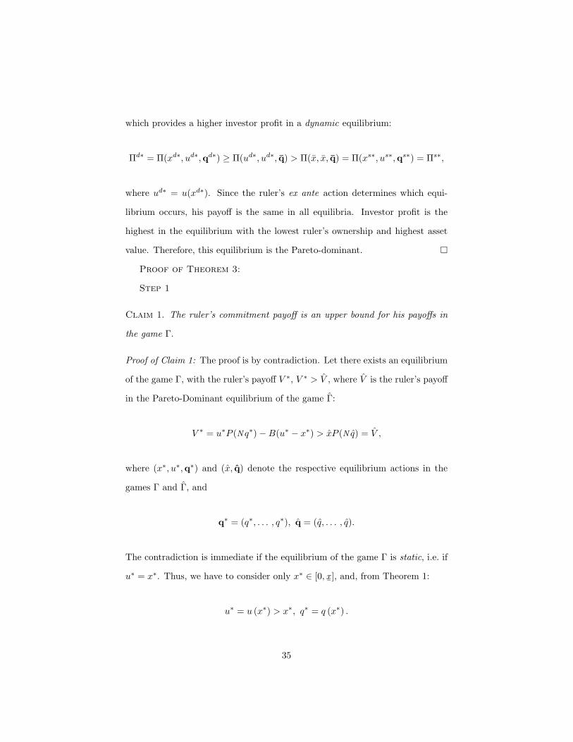
which provides a higher investor profit in a dynamic equilibrium:

Πd∗ = Π(xd∗, ud∗,qd∗) ≥ Π(ud∗, ud∗, q) > Π(x, x, q) = Π(xs∗, us∗,qs∗) = Πs∗,

where ud∗ = u(xd∗). Since the ruler’s ex ante action determines which equi-

librium occurs, his payoff is the same in all equilibria. Investor profit is the

highest in the equilibrium with the lowest ruler’s ownership and highest asset

value. Therefore, this equilibrium is the Pareto-dominant. �

Proof of Theorem 3:

Step 1

Claim 1. The ruler’s commitment payoff is an upper bound for his payoffs in

the game Γ.

Proof of Claim 1: The proof is by contradiction. Let there exists an equilibrium

of the game Γ, with the ruler’s payoff V ∗, V ∗ > V , where V is the ruler’s payoff

in the Pareto-Dominant equilibrium of the game Γ:

V ∗ = u∗P (N q∗)−B(u∗ − x∗) > xP (N q) = V ,

where (x∗, u∗,q∗) and (x, q) denote the respective equilibrium actions in the

games Γ and Γ, and

q∗ = (q∗, . . . , q∗), q = (q, . . . , q).

The contradiction is immediate if the equilibrium of the game Γ is static, i.e. if

u∗ = x∗. Thus, we have to consider only x∗ ∈ [0, x¯], and, from Theorem 1:

u∗ = u (x∗) > x∗, q∗ = q (x∗) .

35

From equation (17), when the equilibrium is dynamic:

q∗ = q(u∗) < q(x∗).

Compute the ruler’s payoff in the game Γ at the action u∗:

V (u∗, q(u∗)) = u∗P (N q(u∗)) > u∗P (N q∗) > V ∗ > V = xP (N q) ,

and, thus, the ruler’s payoff from u∗ in the game Γ is higher than V ∗, which

contradicts to the assumption that V < V ∗ is an equilibrium. �

Step 2

Claim 2. Claim 2. The equilibrium asset value in the game Γ is bounded by

the commitment asset value.

Proof of Claim 2: The statement of Claim 2 is trivial when the equilibrium of

the game Γ is static. Thus, our considerations are limited by dynamic equilibria,

i.e. by the case when the ruler’s ex ante action x ∈ [0, x¯].

The proof of Claim 2 is by contradiction. Let there exist an equilibrium of

the game Γ with q∗ > q, where q∗ = q(x∗) and q = q(x) are the asset values in

the games Γ and Γ with the equilibrium actions (x∗, u∗, q∗) and (x, q). Then,

V (u∗, q(u∗)) ≤ V (x, q(x)),

because V (x, q(x)) is an equilibrium. Consider the ruler’s ex ante action x such

that u(x) = x. Then, the ruler’s payoff Vf (x) is higher than his equilibrium

36

payoff Vf (x∗):

Vf (x) = u(x)P (N q(x))−B(u(x)− x)

= xP (N q(x))−B(x− x) = V ,

Vf (x∗) = u(x∗)P (N q(x∗))−B(u∗ − x∗)

= V (u∗, q(u∗))−B(u∗ − x∗).

From equations (3) and (15) and properties of the function B:

B(u∗ − x∗) > B(x− x),

which provides:

Vf (x) > Vf (x∗),

a contradiction to the assumption that (x∗, u∗, q∗) are the equilibrium actions

of the game Γ. Therefore, q∗ ≤ q. From equation (17) we have q(x) > q(x)

for all x ∈ [0, x). We have proven that such asset value cannot occur in the

equilibrium of the game Γ. Thus, x∗ /∈ [0, x). Differentiate equation (3) and use

of equation (13) to prove that

dy (x)dx

∈ [0, 1] ,

and since x∗ > x, we have:

u∗ = u(x∗) > u(x) = x.

Thus, investor equilibrium profit in the game Γ is bounded by their equilibrium

37

profit in the game Γ: because investor profit is decreasing in their ownership

share. �

Note that we have proven a stronger version of Theorem 3 than we stated in

the main text of this paper. We have shown that the equilibrium asset value in

the game Γ is bounded by the lowest asset value within the set of equilibrium

asset values in the game Γ. We will use this fact in our proof of Theorem 4.

Proof of Theorem 4

Step 1: Let N1 < N2 and compare the games Γ(N1 ) and Γ(N2 ), where

Γ(N ) denotes the game Γ with N investors, and the subscript N is used to

denote the respective game.

Claim 1. In the game Γ(N) the ruler’s equilibrium payoff increases in N.

Proof of Claim 1: When ruler’s ex ante actions in both games are the same,

from equations (4) and (12) aggregate best response investment is higher in the

game Γ(N2 ):

fN1(x)× N1 < fN2(x)× N2 .

By employing ex ante equilibrium action from Γ(N1 ) in Γ(N2 ), the ruler secures

a higher payoff in Γ(N2 ) than his equilibrium payoff in Γ(N1 ), and Claim 1 is

proven. �

Step 2

Lemma 2: When P ′′′ ≤ 0 the equilibrium of the game Γ is unique.

Proof of Lemma 2: When P ′′′ ≤ 0, the ruler’s second order conditions are

negative:

xP ′(Q(x))d2Q(x)

dx2+ xP ′′(Q(x))

[dQ(x)

dx

]2

+ 2P ′(Q(x))dQ(x)

dx< 0 : ∀x ∈ [0, 1],

38

where d2Q(x)dx2 < 0:

d2Q(x)dx2

=2i

(1− x)3A′(Q(x))+

iA′′(Q(x))

(1− x)2[A′(Q(x))

]2 < 0,(25)

because

A′′(Q) =1N

P ′′′(Q) +[1− 1

N

]1Q

(P ′′(Q)− 2

Q

[P ′(Q)− P (Q)

Q

])≤ 0,

due to

P ′′(Q)− 2Q

[P ′(Q)− P (Q)Q

] ≤ 0 if P ′′′(Q) ≤ 0.(26)

Thus, the ruler’s share at which his payoff maximized is unique. Thus, the

equilibrium of the game Γ is unique, and Lemma 2 is proven. �

Claim 2: In the game ΓN equilibrium asset value increases with N :

Proof of Claim 2: Assume the reverse: let QN1 > QN2 . Then, xN1 < xN2 , and

there exits x such that in the game Γ(N2 ):

qN2(x)× N2 = QN1 ,

and

xN1 < x < xN2 .(27)

From Theorem 1 and Lemma 2, in the game Γ(N2 ):

dV (x)dx

∣∣∣∣∣x<xN2

> 0,dV (x)

dx

∣∣∣∣∣x=xN2

= 0,dV (x)

dx

∣∣∣∣∣x>xN2

< 0,

39

thus, at x = x:

dV (x)dx

∣∣∣∣∣x=x

× 1P ′

N1

= xQ′(x) +PN1

P ′N1

> 0, orx

(1− x)2

∣∣∣∣ 1A′

N2(Q)

∣∣∣∣ <PN1

P ′N1

,

(28)

where equation (13) was used. When P ′′′ < 0, from equation (10)

A′N2(Q) > A′

N1(Q),(29)

due to equation (26). Analogously, in the game Γ(N1 ):

dV (x)dx

∣∣∣∣∣x=xN1

= 0, orxN1

(1− xN1)2

∣∣∣∣ 1A′

N1(Q)

∣∣∣∣ =PN1

P ′N1

,

and from equations (27) and (29):

x

(1− x)2

∣∣∣∣ 1A′

N2(Q)

∣∣∣∣ >xN1

(1− xN1)2

∣∣∣∣ 1A′

N1(Q)

∣∣∣∣ ,

which contradicts equation (28), and Claim 2 is proven. �

Step 3

Consider Q ∈ [Q,QN (0)], where QN (0) = qN (0) × N . From the proof of

Theorem 1, for any such Q, there exists a unique subgame of the game ΓN ,

which starts with xN , which aggregate equilibrium investment is Q. Let oN (Q)

denote this equilibrium outcome with actions (xN (Q), yN (Q),qN ), where

qN = Q/N and qN = q(yN ), qN = q(xN (Q)).

From our construction and Theorem 1, yN (Q) is an inverse to Q(yN ) and

xN (Q) – to Q(xN ), and the functions yN and xN are well-defined for Q ∈

40

[Q,QN (0)].

Claim 3: For N1 < N2 and Q ∈ [Q, QN1(0)] we have:

d[xN2(Q)− xN1(Q)]dQ

> 0 if N1 < N2 and Q ∈ [Q,QN1(0)].(30)

Proof of Claim 3: Since N1 < N2, for any fixed Q ∈ [Q,QN1(0)] we have:

xN1 < xN2 and yN1 < yN2, or (1− yN2(Q)) < (1− yN1(Q)),

and using equations (11) and (29) we get:

∣∣∣∣dQN1(x)dx

∣∣∣∣x=xN1(Q)

<

∣∣∣∣dQN2(x)dx

∣∣∣∣x=xN2(Q)

,

which is the same as equation (30), because it can be written as:

1∣∣∣dQN1(x)dx

∣∣∣x=xN1(Q)

− 1∣∣∣dQN2(x)dx

∣∣∣x=xN2(Q)

> 0,

and Claim 3 is proven. �

Step 4

Lemma 4: If the equilibrium outcome o∗N of the game ΓN is static, but is not a

commitment outcome, we have: Q∗N = N × qN (x∗) = Q, and x∗ is determined

from G(x∗) = 0, i.e., x∗ = x.

Proof of Lemma 4: Follows from the proof of Theorem 1. �

Claim 4: In the game Γ(N ) aggregate equilibrium investment Q∗ = q∗N ×N is

non-decreasing in N :

Q∗N1 ≤ Q∗

N2 if N1 < N2(31)

41

Proof of Claim 4: If the commitment outcomes are sustainable in the games

Γ(N1 ) and Γ(N2 ), equation (31) follows from Claim 2. Let the outcomes o∗N1

and o∗N2 with actions (x∗N1, y∗N1,q

∗N1) and (x∗N2, y

∗N2,q

∗N2) be equilibria of the

games Γ(N1 ) and Γ(N2 ), and Q∗N1 > Q∗

N2 in violation of equation (31). If both

games have static equilibria, equation (31) is immediate from Lemma 4. Thus, if

Q∗N1 > Q∗

N2 holds, the equilibrium of the game ΓN1 is dynamic. Let the outcome

oN1 with actions (xN1, yN1, qN1) and qN1 = Q∗N2/N1, and the outcome oN2

with actions (xN2, yN2, qN2) and qN2 = Q∗N1/N2, denote the equilibria of the

subgames of the games Γ(N1 ) and Γ(N2 ) that start with actions xN1 and xN2,

respectively. From Theorem 1, oN1 and oN2 exist and are unique, and:

Q(xN1) = Q∗N2 and Q(xN2) = Q∗

N1,

Q(yN1) = Q∗N2 and Q(yN2) = Q∗

N1,

x∗N1 < xN1 < x∗N2 and x∗N1 < xN2 < x∗N2.

From our construction:

VN2 − V ∗N1 = (yN1 − y∗N1)×Q∗

N1 = (xN1 − x∗N1)×Q∗N1,

V ∗N2 − VN1 = (y∗N2 − yN1)×Q∗

N1 = (x∗N2 − xN1)×Q∗N1,

where VN1, VN2 and V ∗N1, V ∗

N2 denote the ruler’s payoffs from outcomes oN1,

oN2, and o∗N1, o∗N2 in the respective games. From equation (30):

VN2 − V ∗N1 > V ∗

N2 − VN1,

42

because Q∗N1 > Q∗

N2. We rearrange the last equation as:

VN2 − V ∗N2 > V ∗

N1 − VN1.(32)

Since the ruler’s payoff is the highest in equilibrium:

V ∗N1 − VN1 > 0,

and from equation (32):

VN2 − V ∗N2 > 0,

which contradicts the assumption that o∗N2 is an equilibrium of the game Γ(N2 ).

Thus, equation (31) holds, and Claim 4 and Theorem 4 are proven. �

University of Michigan, Ann Arbor

References

[1] Anderlini, Luca and Felli, Leonardo, “Costly Coasian Contracts,” CARESS

Working paper, (1997), 97-111.

[2] Coase, Ronald, “The Problem of Social Cost,” Journal of Law and Eco-

nomics, Vol. 3, (1960), 1-44.

[3] Davies, David, “Property Rights and Economic Efficiency: the Australian

Airlines Revised,” Journal of Law and Economics, 20, (1977), 223-226.

[4] Derthick, Martha, Agency under Stress: The Social Security Administra-

tion in American Government, Brookings Institution: Washington, D.C.,

1990.

[5] Clarkson, Andrew, Princeton University Ph. D. Thesis, 1996.

43

[6] Dixit, Avinash K., “Power of Incentives in Private Versus Public Organiza-

tions,” American Economic Review, 87(2), (1997), 378-382.

[7] Greif, Avner, “Economic History and Game Theory: a Survey,” Handbook

of Game Theory, Vol. III, in Aumann, Robert J. and Hart, Sergiu, eds.,

North Holland: Amsterdam, 1996.

[8] Hart, Oliver D. and Moore, John, “Incomplete Contracts and Renegotia-

tion,” Econometrica, 56(4), (1988), 755-785.

[9] Joskow, Paul and Noll, Roger G., “American Economic Policy in the 1980s,”

in Feldstein, Martin, ed., NBER Conference Report, The University of

Chicago Press, Ltd: London, (1994), 367-440.

[10] Laffont, Jean-Jacques and Tirole, Jean J., A Theory of Incentives in Pro-

curement of Regulation, 2nd ed., The MIT Press: Cambridge, Mas-

sachusetts, 1994.

[11] Noll, Roger, “The Politics of Regulation,” Handbook of Industrial Organi-

zation, Vol. II, in Schmalensee Richard and Willig, Robert, eds., North

Holland: Amsterdam, 1989.

[12] McNeil, William H., History of Western Civilization, A Handbook, The

University of Chicago Press, Ltd: London, 1986.

[13] Osborne, Martin J. and Rubinstein, Ariel, A Course in Game Theory, The

MIT Press: Cambridge, Massachusetts, 1994.

[14] Rubinstein, Ariel, “Perfect Equilibrium in a Bargaining Model,” Econo-

metrica, 50, (1982), 97-109.

[15] Russel, Bertrand, Power: A New Social Analysis, London: George Allen

& Unwin; New York: W.W. Norton, 1938. Reprint edition: Routledge,

1993.

44

[16] Sachs, Jeffrey D. and Pistor, Katharina, “The Rule of Law and Economic

Reform in Russia,” John M. Olin Critical Issues Series, in Sachs, Jeffrey

D. and Pistor, Katharina, eds., Harper Collins, Westview Press: Boulder

and Oxford, 1997.

[17] Schwartz, Galina, “ Non-Enforceability of Trade Treaties and the Most-

Favored Nation Clause: a Game Theoretic Analysis of Investment Dis-

tortions,” Princeton University Ph.D. Dissertation, 2000.

[18] Shleifer, Andre, Lopez de Silanes, Florencio, La Porta, Rafael and Vishny,

Robert, “Law and Finance,” Journal of Political Economy, 106(6),

(1998), 1113-1155.

[19] Shapiro, Carl and Willig, Robert D., “Economic Rationales for the Scope

of Privatization.” The Political Economy of Public Sector Reform and

Privatization, in Suleiman E. and Waterbury, J. eds., Westview Press:

London, (1990), 55-87.

[20] Staiger, Robert, “International Rules and Institutions for Trade Policy,”

Handbook of International Economics, vol. III, in Grossman Gene and

Rogoff Kenneth, eds., North Holland: Amsterdam, 1995.

[21] Tirole, Jean, “Incomplete contracts: Where do we stand?,” Econometrica,

67(4), (1999), 741-781.

[22] Wilson, James Q., Bureaucracy: What Government Agencies Do and Why

They Do It, Basic Books: New York, 1989.

45