Continuum Mechanics

Fridtjov Irgens

Continuum Mechanics

With 279 Figures and 4 Tables

Fridtjov Irgens

Wolffsgate 125006 BergenNorwayfridtjov.irgens@ntnu.no

ISBN: 978-3-540-74297-5 e-ISBN: 978-3-540-74298-2

Library of Congress Control Number: 2007936609

c© 2008 Springer-Verlag Berlin Heidelberg

This work is subject to copyright. All rights are reserved, whether the whole or part of the material isconcerned, specifically the rights of translation, reprinting, reuse of illustrations, recitation, broadcasting,reproduction on microfilm or in any other way, and storage in data banks. Duplication of this publicationor parts thereof is permitted only under the provisions of the German Copyright Law of September 9,1965, in its current version, and permission for use must always be obtained from Springer. Violations areliable to prosecution under the German Copyright Law.

The use of general descriptive names, registered names, trademarks, etc. in this publication does not imply,even in the absence of a specific statement, that such names are exempt from the relevant protective lawsand regulations and therefore free for general use.

Cover Design: Steinen-Broo, e Studio Calamar, Girona

Printed on acid-free paper

9 8 7 6 5 4 3 2 1

springer.com

Preface

Students of engineering and engineering science are early in their studies exposed toApplied Mechanics: Statics and Dynamics of rigid bodies, Strength of Materials andFluid Mechanics. As a teacher of these subjects for many years at the NorwegianUniversity of Science and Technology, and for students of most special branchesof engineering, I have found that it is highly relevant and important that studentswho want to obtain a better understanding of the mechanics of materials or of themechanics of fluids, should take a course in Continuum Mechanics, a discipline thatsynthesizes the basic concepts of the mechanics of solids and fluids.

The pioneers in natural science were experts in many different disciplines ofphysics and mechanics. Leonhard Euler [1707–1783] is an example of a scientistwho has made permanent contributions both in Solid Mechanics: the Euler theoryof column buckling, and Fluid Mechanics: the Euler equations of inviscid fluids.Later came times when special fields like the Theory of Elasticity, Hydrodynamics,and Gas Dynamics dominated. Classical Theory of Elasticity is the mechanics ofisotropic and linearly elastic materials, for which the behavior is based on extensionsof Hooke’s law, and where deformations are assumed to be small. Hydrodynamicsis the mechanics of liquids, and Gas Dynamics is the thermomechanics of gasses.These two disciplines are joined in the science of Fluid Mechanics, the term fluidbeing a common name for liquids and gasses.

Although these separate parts of mechanics still exist as important special fields,a need for unification of the mechanics of solids and fluids became important inmodern times, let us say in the last 60 years or so. New and complex materialshave been invented and made available, and a better utilization of the materials hasbecome necessary or important. The fundamental distinctions between the thermo-mechanical behavior of liquids and solid materials are no longer clear. Solid ma-terials behave fluid-like in many forming processes, although they still are in thesolid phase, and these forming processes need to be analyzed and modelled. Mod-ern engineering materials may exhibit linear or non-linear elastic, viscous, plastic,viscoelastic, viscoplastic, or visco-elasto-plastic behavior.

Another reason for the importance of understanding properly the thermomechan-ical behavior of advanced materials is the development of numerical methods and

v

vi Preface

the existence of highly advanced and speedy computers, which may be used to pro-vide solutions of problems involving complex geometries and very complex ther-momechanical material behavior.

The study of distributions of energy, matter, and other physical quantities undercircumstances where their discrete nature is unimportant, and where they may be re-garded as continuous functions of position and time, is called Classical Field Theoryor Continuum Physics. This branch of Physics presumes nothing directly regardingthe structure of the materials, although the structure of a material may be reflectedin the way the physical quantities are described. When the physical quantities arepurely of mechanical or thermodynamical nature, the subject is called ContinuumMechanics.

Continuum Mechanics is based on the continuum hypothesis: Matter is contin-uously distributed throughout the space occupied by the matter. Regardless of howsmall volume elements the matter is subdivided into, every element will containmatter. The basis for the hypothesis is how we directly experience matter and itsmacroscopic properties, and furthermore on how physical quantities we use, as forexample pressure, temperature, and velocity, are measured macroscopically.

The material in this book has evolved from my lecture notes produced duringmany years of teaching undergraduate courses and graduate courses in Mechanicsof materials, Continuum Mechanics, Tensor Analysis, Rheology, and Biomechanics.The book is a textbook designed for classroom teaching or self-study. Most of thechapters conclude with exercise problems.

The references at the end of the book present the major sources during my studyof the subject of Continuum Mechanics. Extensive bibliographies from the timebefore 1965 may be found in the important treatises by Truesdell and Toupin [54]and Truesdell and Noll [53].

A short presentation of the contents of the book. Chapter 1 presents some of thebasic concepts of macromechanical properties of materials when they are consideredto be continuous matter: normal stress, shear stress, longitudinal strain and shearstrain. The simplest equations relating these quantities are discussed, e.g. Hooke’slaw relating normal stress and longitudinal strain in an elastic material, and New-ton’s law of fluid friction relating shear stress and shear strain rate.

Chapter 2 presents some basic mathematical concepts: matrix algebra, vectoralgebra and vector analysis. Vectors are presented using index notation, i.e. throughvector components in a Cartesian coordinate system, by collecting the componentsin vector matrices, i.e. the index free notation, and finally by the coordinate invariantand bold face notation.

Chapter 3 contains the basic Continuum Mechanics: Kinematics, Kinetics withthe equations of motion for bodies and material points, and General Stress Anal-ysis, common to all continuous materials. The concept of tensors is introduced bydefining the stress tensor as a coordinate invariant quantity.

Chapter 4 presents tensors as coordinate invariant quantities through multilin-ear scalar-valued functions of vectors, alternatively expressed by their componentsin Cartesian coordinates. The formal presentation of tensor analysis expressed bycomponents in general curvilinear coordinates is postponed to Chap. 12.

Preface vii

The analysis of small and large deformations and strains is the subject of Chap. 5.The analysis of strain rates, rates of deformation, and rates of rotations, of majorimportance in Fluid Mechanics and in describing rate dependent materials, is alsoincluded in this chapter.

Chapter 6 discusses the concepts work, power, and energy. The mechanical en-ergy balance equation and the thermal energy balance equation, which is based onthe first law of thermodynamics, are presented. The second law of thermodynamicsis given a brief presentation. Some consequences of this law in constitutive mod-elling are given in Chap. 11.

Chapter 7 is an extensive exposition of the classical theory of isotropic, lin-early elastic materials. Many important applications in two-dimensional theory aretreated, and the chapter gives a comprehensive discussion on elastic waves. A sec-tion on anisotropic elastic materials having different degrees of symmetries servesas an introduction to fiber composite materials. Finite elasticity is briefly presented.

Chapter 8 has sections on perfect fluids, linearly viscous fluids, potential flow,and non-Newtonian fluid models. Advanced non-Newtonian fluids are presented inChap. 9 and in Chap. 11.

Chapter 9 presents the theory of viscoelasticity for both solids and fluids.Chapter 10 contains some basic parts of the theory of plasticity. The criteria

for yielding and the yield laws or flow rules are presented for the most commonlyused material models. The important theorems for upper and lower bound solutionsfor elastoplastic materials are presented. Viscoplasticity, which combines plasticbehaviour with viscous response at yielding, is given a brief presentation. Finallythe yield line theory is presented.

Principles and theories for the mathematical modelling of materials is the maintheme in Chap. 11. An extension of the deformation analysis from Chap. 5 and theconcepts of objective tensors and corotational time derivative are presented and dis-cussed. Non-linear materials with elastic, viscous, viscoelastic, plastic, viscoplasticand viscoelastic-plastic responses are discussed.

Chapter 12 presents the components of tensors in general curvilinear coordinatesystems in the 3-dimensional physical Euclidean space E3. The concept of tensorsis the same as in Chap. 4, but is now extended to more general coordinate systems.

Chapter 13 provides the general field equations of Continuum Mechanics incurvilinear coordinates. Concepts like convected coordinates and the related defor-mation analysis are introduced. The concept of convected time derivatives is givengeometrically definitions.

The present book was originally presented in Norwegian and in three parts: PartI Continuum Mechanics, Part II Mechanics of Materials (Constitutive Modelling),and Part III Tensor Analysis (Curvilinear coordinates in continuum mechanics). PartI was published by Tapir Akademisk Forlag in 1974, and Part III was published in1982 by the same publishers. Part II was only presented in a compendium form.The reason for this was that I found that the extension of the theme and the contin-ued developments within the science of constitutive modelling made it difficult tochoose and limit the content properly. Part I and II have since gone through many

viii Preface

and extensive revisions and have been presented as departmental compendiums in anumber of editions. In 2000–2001 the compendiums were translated into English.

Each of the three parts of the book was meant to cover the course material in ad-vanced semester courses. Part I contained: The Foundation of Continuum Mechan-ics using tensors in Cartesian coordinate systems, Classical Theory of Elasticity,and Fluid Mechanics. Part II had chapters on Viscoelasticity, Plasticity, Principlesof Constitutive Modelling, and Thermodynamics. Part III presented Tensor Analysisin curvilinear coordinates and the fundamental equations of Continuum Mechanicsin these coordinates.

In the present English version of the book the three parts are put together in onevolume. The intentions of the first version of the book have been retained, whichmeans that the book may be used as a text book in more than one course. I willsuggest four different courses:

Course 1. An introductory course in Continuum Mechanics. Contents: Funda-mental equations of Kinematics and Kinetics applied in Continuum Mechanics,Analysis of Stress, Small Deformations, and Rates of Deformation, Tensor Anal-ysis using Cartesian coordinates, Linear Elasticity, Fluid Mechanics. The coursemay be based upon the material in Chaps. 1, 2, 3, Sect. 4.1–3, 5.1–4, 6.1.1, 7.1–3,7.5, 7.7.1–3, 8.1, 8.3 (except 8.3.1–3), 8.4.1–2.

Course 2. Advanced Mechanics of Materials. This course is a continuation ofCourse 1 and includes: Anisotropic Elasticity, Composite Materials, Viscoelasticity,and Plasticity. The course may be based upon the materials in Sect. 7.8 and 7.9,Chaps. 9 and 10.

Course 3. A graduate course in Continuum Mechanics. Contents: Foundationof Continuum Mechanics, Analysis of Stress, Small and Large Deformations, andRates of Deformation, Tensor Analysis using Cartesian coordinates, Linear andNon-linear Theory of Elasticity, Fluid Mechanics, Non-Newtonian Fluids, Vis-coelasticity, and Plasticity, Principles of Constitutive Modelling. The course maybe based upon the materials in Chaps. 1–11.

Course 4. Tensor Analysis. The course presents tensors as applied in ContinuumMechanics. The tensors are defined as invariant quantities with respect to coordinatesystems but presented by components in both Cartesian systems and in curvilinearcoordinate systems. The course may be based upon material from Chaps. 1, 2, 3,4, 5, Sect. 6.1, 7.1–2, 7.5, 7.6, 7.7.1–3, 8.1, 8.3 (except Sect. 8.3.1–3), 8.4.1–2, andChaps. 12, and 13.

During my study of general Mechanics and Continuum Mechanics I have re-ceived many comments and suggestions from colleagues at Department of AppliedMechanics, Thermodynamics, and Fluid Dynamics and Department of StructuralEngineering, both at Norwegian University of Science and Technology. In par-ticular I will thank professor Arvid Gustafson, professor Jan B. Aarseth, profes-sor Henry Øiann, and professor Leif Rune Hellevik, and from my former studentsDr. Geir Berge and professor Per Olaf Tjelflaat for their valuable contributions.

As visiting professor at University of Connecticut and University of Colorado Ihave received many impulses from American colleagues. In particular I will like tothank professor Kaspar Willam and professor Stein Sture for their hospitality during

Preface ix

my sabbaticals in 1990–91 and in 2000 at Department of Civil, Environmental, andArchitectural Engineering, University of Colorado at Boulder.

Siv.ing. Lars Haga and stud. techn. Marthe Sæther have produced most of thefigures in the book, and I thank them for their contributions.

Finally, thanks to my wife Eva, who has supported and encouraged me.

Bergen, October, 2007 Fridtjov Irgens

Contents

1 Introduction . . . . . . . . . . . . . . . . . . . . . . . . . . . . . . . . . . . . . . . . . . . . . . . . . . . 11.1 The Continuum Hypothesis . . . . . . . . . . . . . . . . . . . . . . . . . . . . . . . . . 11.2 Elasticity, Plasticity, and Fracture . . . . . . . . . . . . . . . . . . . . . . . . . . . . 21.3 Fluids . . . . . . . . . . . . . . . . . . . . . . . . . . . . . . . . . . . . . . . . . . . . . . . . . . . 81.4 Viscoelasticity . . . . . . . . . . . . . . . . . . . . . . . . . . . . . . . . . . . . . . . . . . . . 121.5 An Outline for the Present Book . . . . . . . . . . . . . . . . . . . . . . . . . . . . . 16

2 Mathematical Foundation . . . . . . . . . . . . . . . . . . . . . . . . . . . . . . . . . . . . . . . 192.1 Matrices and Determinants . . . . . . . . . . . . . . . . . . . . . . . . . . . . . . . . . 192.2 Coordinate Systems and Vectors . . . . . . . . . . . . . . . . . . . . . . . . . . . . . 232.3 Coordinate Transformations . . . . . . . . . . . . . . . . . . . . . . . . . . . . . . . . 282.4 Scalar Fields and Vector Fields . . . . . . . . . . . . . . . . . . . . . . . . . . . . . . 30Problems . . . . . . . . . . . . . . . . . . . . . . . . . . . . . . . . . . . . . . . . . . . . . . . . . . . . . . 34

3 Dynamics . . . . . . . . . . . . . . . . . . . . . . . . . . . . . . . . . . . . . . . . . . . . . . . . . . . . . 373.1 Kinematics . . . . . . . . . . . . . . . . . . . . . . . . . . . . . . . . . . . . . . . . . . . . . . . 37

3.1.1 Lagrangian Coordinates and Eulerian Coordinates . . . . . . 373.1.2 Material Derivative of an Intensive Quantity . . . . . . . . . . . . 403.1.3 Material Derivative of an Extensive Quantity . . . . . . . . . . . 41

3.2 Equations of Motion . . . . . . . . . . . . . . . . . . . . . . . . . . . . . . . . . . . . . . . 423.2.1 Euler’s Axioms . . . . . . . . . . . . . . . . . . . . . . . . . . . . . . . . . . . . 423.2.2 Newton’s 3. Law . . . . . . . . . . . . . . . . . . . . . . . . . . . . . . . . . . 463.2.3 Coordinate Stresses . . . . . . . . . . . . . . . . . . . . . . . . . . . . . . . . 473.2.4 Cauchy’s Stress Theorem and Cauchy’s Stress Tensor . . . 503.2.5 Cauchy Equations of Motion . . . . . . . . . . . . . . . . . . . . . . . . 543.2.6 Alternative Derivation of the Cauchy Equations . . . . . . . . . 58

3.3 Stress Analysis . . . . . . . . . . . . . . . . . . . . . . . . . . . . . . . . . . . . . . . . . . . 603.3.1 Principal Stresses . . . . . . . . . . . . . . . . . . . . . . . . . . . . . . . . . . 603.3.2 Stress Deviator and Stress Isotrop . . . . . . . . . . . . . . . . . . . . 653.3.3 Extremal Values for Normal Stress . . . . . . . . . . . . . . . . . . . 683.3.4 Maximum Shear Stress . . . . . . . . . . . . . . . . . . . . . . . . . . . . . 69

xi

xii Contents

3.3.5 Plane Stress . . . . . . . . . . . . . . . . . . . . . . . . . . . . . . . . . . . . . . . 703.3.6 Mohr Diagram for Plane Stress . . . . . . . . . . . . . . . . . . . . . . 733.3.7 Mohr Diagram for General States of Stress . . . . . . . . . . . . . 77

Problems . . . . . . . . . . . . . . . . . . . . . . . . . . . . . . . . . . . . . . . . . . . . . . . . . . . . . . 79

4 Tensors . . . . . . . . . . . . . . . . . . . . . . . . . . . . . . . . . . . . . . . . . . . . . . . . . . . . . . . 834.1 Definition of Tensors . . . . . . . . . . . . . . . . . . . . . . . . . . . . . . . . . . . . . . 834.2 Tensor Algebra . . . . . . . . . . . . . . . . . . . . . . . . . . . . . . . . . . . . . . . . . . . 89

4.2.1 Isotropic Tensors of 4. Order . . . . . . . . . . . . . . . . . . . . . . . . 944.2.2 Tensors as Polyadics . . . . . . . . . . . . . . . . . . . . . . . . . . . . . . . 96

4.3 Tensors of 2. Order. Part One . . . . . . . . . . . . . . . . . . . . . . . . . . . . . . . 974.3.1 Symmetric Tensors of 2. Order . . . . . . . . . . . . . . . . . . . . . . . 1004.3.2 Alternative Invariants . . . . . . . . . . . . . . . . . . . . . . . . . . . . . . . 1034.3.3 Deviator and Isotrop . . . . . . . . . . . . . . . . . . . . . . . . . . . . . . . 104

4.4 Tensor Fields . . . . . . . . . . . . . . . . . . . . . . . . . . . . . . . . . . . . . . . . . . . . . 1054.4.1 Gradient, Divergence, and Rotation . . . . . . . . . . . . . . . . . . . 1054.4.2 Del-Operator . . . . . . . . . . . . . . . . . . . . . . . . . . . . . . . . . . . . . . 1074.4.3 Orthogonal Coordinates . . . . . . . . . . . . . . . . . . . . . . . . . . . . . 1084.4.4 Material Derivative of a Tensor Field . . . . . . . . . . . . . . . . . . 110

4.5 Rigid-Body Dynamics . . . . . . . . . . . . . . . . . . . . . . . . . . . . . . . . . . . . . 1114.5.1 Kinematics . . . . . . . . . . . . . . . . . . . . . . . . . . . . . . . . . . . . . . . 1124.5.2 Relative Motion . . . . . . . . . . . . . . . . . . . . . . . . . . . . . . . . . . . 1174.5.3 Kinetics . . . . . . . . . . . . . . . . . . . . . . . . . . . . . . . . . . . . . . . . . . 119

4.6 Tensors of 2. Order. Part Two . . . . . . . . . . . . . . . . . . . . . . . . . . . . . . . 1224.6.1 Rotation of Vectors and Tensors . . . . . . . . . . . . . . . . . . . . . . 1234.6.2 Polar Decomposition . . . . . . . . . . . . . . . . . . . . . . . . . . . . . . . 1244.6.3 Isotropic Functions of Tensors . . . . . . . . . . . . . . . . . . . . . . . 125

Problems . . . . . . . . . . . . . . . . . . . . . . . . . . . . . . . . . . . . . . . . . . . . . . . . . . . . . . 129

5 Deformation Analysis . . . . . . . . . . . . . . . . . . . . . . . . . . . . . . . . . . . . . . . . . . . 1335.1 Strain Measures . . . . . . . . . . . . . . . . . . . . . . . . . . . . . . . . . . . . . . . . . . . 1335.2 The Green Strain Tensor . . . . . . . . . . . . . . . . . . . . . . . . . . . . . . . . . . . 1345.3 Small Strains and Small Deformations . . . . . . . . . . . . . . . . . . . . . . . . 139

5.3.1 Small Strains . . . . . . . . . . . . . . . . . . . . . . . . . . . . . . . . . . . . . . 1405.3.2 Small Deformations . . . . . . . . . . . . . . . . . . . . . . . . . . . . . . . . 1415.3.3 Coordinate Strains in Cylindrical Coordinates and

Spherical Coordinates . . . . . . . . . . . . . . . . . . . . . . . . . . . . . . 1425.3.4 Principal Strains and Principal Directions of Strains . . . . . 1445.3.5 Strain Isotrop and Strain Deviator . . . . . . . . . . . . . . . . . . . . 1455.3.6 Rotation Tensor for Small Deformations . . . . . . . . . . . . . . . 1455.3.7 Small Strains in a Material Surface . . . . . . . . . . . . . . . . . . . 1475.3.8 Mohr Diagram for Strain . . . . . . . . . . . . . . . . . . . . . . . . . . . . 1485.3.9 Equations of Compatibility . . . . . . . . . . . . . . . . . . . . . . . . . . 1485.3.10 Compatibility Equations as Sufficient Conditions . . . . . . . 150

5.4 Rates of Deformation, Strain, and Rotation . . . . . . . . . . . . . . . . . . . . 151

Contents xiii

5.4.1 Rate of Deformation Matrix and Rate of RotationMatrix in Cylindrical and Spherical Coordinates . . . . . . . . 158

5.5 Large Deformations . . . . . . . . . . . . . . . . . . . . . . . . . . . . . . . . . . . . . . . 1605.5.1 Special Types of Deformations and Flows . . . . . . . . . . . . . 1665.5.2 The Continuity Equation in a Particle . . . . . . . . . . . . . . . . . 1725.5.3 Reduction to Small Deformations . . . . . . . . . . . . . . . . . . . . 1725.5.4 Deformation with Respect to the Present Configuration . . 173

5.6 The Piola-Kirchhoff Stress Tensors . . . . . . . . . . . . . . . . . . . . . . . . . . 175Problems . . . . . . . . . . . . . . . . . . . . . . . . . . . . . . . . . . . . . . . . . . . . . . . . . . . . . . 178

6 Work and Energy . . . . . . . . . . . . . . . . . . . . . . . . . . . . . . . . . . . . . . . . . . . . . . 1836.1 Mechanical Energy Balance . . . . . . . . . . . . . . . . . . . . . . . . . . . . . . . . 183

6.1.1 The Work-Energy Equation for Rigid Bodies . . . . . . . . . . . 1866.1.2 Conjugate Stress Tensors and Deformation Tensors . . . . . . 189

6.2 The Principle of Virtual Power . . . . . . . . . . . . . . . . . . . . . . . . . . . . . . 1906.3 Thermal Energy Balance . . . . . . . . . . . . . . . . . . . . . . . . . . . . . . . . . . . 192

6.3.1 Thermodynamic Introduction . . . . . . . . . . . . . . . . . . . . . . . . 1926.3.2 Thermal Energy Balance . . . . . . . . . . . . . . . . . . . . . . . . . . . . 193

6.4 The Second Law of Thermodynamics . . . . . . . . . . . . . . . . . . . . . . . . 195Problems . . . . . . . . . . . . . . . . . . . . . . . . . . . . . . . . . . . . . . . . . . . . . . . . . . . . . . 198

7 Theory of Elasticity . . . . . . . . . . . . . . . . . . . . . . . . . . . . . . . . . . . . . . . . . . . . 1997.1 Introduction . . . . . . . . . . . . . . . . . . . . . . . . . . . . . . . . . . . . . . . . . . . . . . 1997.2 The Hookean Solid . . . . . . . . . . . . . . . . . . . . . . . . . . . . . . . . . . . . . . . . 200

7.2.1 An Alternative Development of the GeneralizedHooke’s Law . . . . . . . . . . . . . . . . . . . . . . . . . . . . . . . . . . . . . . 205

7.2.2 Strain Energy . . . . . . . . . . . . . . . . . . . . . . . . . . . . . . . . . . . . . 2067.3 Two-Dimensional Theory of Elasticity . . . . . . . . . . . . . . . . . . . . . . . . 207

7.3.1 Plane Stress . . . . . . . . . . . . . . . . . . . . . . . . . . . . . . . . . . . . . . . 2077.3.2 Plane Displacements . . . . . . . . . . . . . . . . . . . . . . . . . . . . . . . 2137.3.3 Airy’s Stress Function . . . . . . . . . . . . . . . . . . . . . . . . . . . . . . 2177.3.4 Airy’s Stress Function in Polar Coordinates . . . . . . . . . . . . 2237.3.5 Axial Symmetry . . . . . . . . . . . . . . . . . . . . . . . . . . . . . . . . . . . 229

7.4 Torsion of Cylindrical Bars . . . . . . . . . . . . . . . . . . . . . . . . . . . . . . . . . 2327.4.1 The Coulomb Theory of Torsion . . . . . . . . . . . . . . . . . . . . . 2327.4.2 The Saint-Venant Theory of Torsion . . . . . . . . . . . . . . . . . . 2347.4.3 Prandtl’s Stress Function . . . . . . . . . . . . . . . . . . . . . . . . . . . . 2387.4.4 The Membrane Analogy . . . . . . . . . . . . . . . . . . . . . . . . . . . . 241

7.5 Thermoelasticity . . . . . . . . . . . . . . . . . . . . . . . . . . . . . . . . . . . . . . . . . . 2447.5.1 Constitutive Equations . . . . . . . . . . . . . . . . . . . . . . . . . . . . . . 2447.5.2 Plane Stress . . . . . . . . . . . . . . . . . . . . . . . . . . . . . . . . . . . . . . . 2457.5.3 Plane Displacements . . . . . . . . . . . . . . . . . . . . . . . . . . . . . . . 248

7.6 Hyperelasticity . . . . . . . . . . . . . . . . . . . . . . . . . . . . . . . . . . . . . . . . . . . 2497.6.1 Elastic Energy . . . . . . . . . . . . . . . . . . . . . . . . . . . . . . . . . . . . . 2497.6.2 The Basic Equations of Hyperelasticity . . . . . . . . . . . . . . . . 252

xiv Contents

7.6.3 The Uniqueness Theorem . . . . . . . . . . . . . . . . . . . . . . . . . . . 2587.7 Stress Waves in Elastic Materials . . . . . . . . . . . . . . . . . . . . . . . . . . . . 260

7.7.1 Longitudinal Waves in Cylindrical Bars . . . . . . . . . . . . . . . 2607.7.2 The Hopkinson Experiment . . . . . . . . . . . . . . . . . . . . . . . . . 2667.7.3 Plane Elastic Waves . . . . . . . . . . . . . . . . . . . . . . . . . . . . . . . . 2687.7.4 Elastic Waves in an Infinite Medium . . . . . . . . . . . . . . . . . . 2707.7.5 Seismic Waves . . . . . . . . . . . . . . . . . . . . . . . . . . . . . . . . . . . . 2707.7.6 Reflection of Elastic Waves . . . . . . . . . . . . . . . . . . . . . . . . . . 2717.7.7 Tensile Fracture Due to Compression Wave . . . . . . . . . . . . 2727.7.8 Surface Waves. Rayleigh Waves . . . . . . . . . . . . . . . . . . . . . . 273

7.8 Anisotropic Materials . . . . . . . . . . . . . . . . . . . . . . . . . . . . . . . . . . . . . . 2747.8.1 Hyperelasticity . . . . . . . . . . . . . . . . . . . . . . . . . . . . . . . . . . . . 2767.8.2 Materials with one Plane of Symmetry . . . . . . . . . . . . . . . . 2777.8.3 Three Orthogonal Symmetry Planes. Orthotropy . . . . . . . . 2797.8.4 Transverse Isotropy . . . . . . . . . . . . . . . . . . . . . . . . . . . . . . . . 2817.8.5 Isotropy . . . . . . . . . . . . . . . . . . . . . . . . . . . . . . . . . . . . . . . . . . 283

7.9 Composite Materials . . . . . . . . . . . . . . . . . . . . . . . . . . . . . . . . . . . . . . . 2847.9.1 Lamina . . . . . . . . . . . . . . . . . . . . . . . . . . . . . . . . . . . . . . . . . . 2857.9.2 From Lamina Axes to Laminate Axes . . . . . . . . . . . . . . . . . 2887.9.3 Engineering Parameters Related to Laminate Axes . . . . . . 2907.9.4 Plate Laminate of Unidirectional Laminas . . . . . . . . . . . . . 290

7.10 Large Deformations . . . . . . . . . . . . . . . . . . . . . . . . . . . . . . . . . . . . . . . 2927.10.1 Isotropic Elasticity . . . . . . . . . . . . . . . . . . . . . . . . . . . . . . . . . 2937.10.2 Hyperelasticity . . . . . . . . . . . . . . . . . . . . . . . . . . . . . . . . . . . . 294

Problems . . . . . . . . . . . . . . . . . . . . . . . . . . . . . . . . . . . . . . . . . . . . . . . . . . . . . . 297

8 Fluid Mechanics . . . . . . . . . . . . . . . . . . . . . . . . . . . . . . . . . . . . . . . . . . . . . . . 3038.1 Introduction . . . . . . . . . . . . . . . . . . . . . . . . . . . . . . . . . . . . . . . . . . . . . . 3038.2 Control Volume. Reynolds’ Transport Theorem . . . . . . . . . . . . . . . . 306

8.2.1 Alternative Derivation of the Reynolds’ TransportTheorem . . . . . . . . . . . . . . . . . . . . . . . . . . . . . . . . . . . . . . . . . 309

8.2.2 Control Volume Equations . . . . . . . . . . . . . . . . . . . . . . . . . . 3108.2.3 Continuity Equation . . . . . . . . . . . . . . . . . . . . . . . . . . . . . . . . 312

8.3 Perfect Fluid ≡ Eulerian Fluid . . . . . . . . . . . . . . . . . . . . . . . . . . . . . . 3138.3.1 Bernoulli’s Equation . . . . . . . . . . . . . . . . . . . . . . . . . . . . . . . 3158.3.2 Circulation and Vorticity . . . . . . . . . . . . . . . . . . . . . . . . . . . . 3198.3.3 Sound Waves . . . . . . . . . . . . . . . . . . . . . . . . . . . . . . . . . . . . . 322

8.4 Linearly Viscous Fluid = Newtonian Fluid . . . . . . . . . . . . . . . . . . . . 3238.4.1 Constitutive Equations . . . . . . . . . . . . . . . . . . . . . . . . . . . . . . 3238.4.2 The Navier-Stokes Equations . . . . . . . . . . . . . . . . . . . . . . . . 3308.4.3 Dissipation . . . . . . . . . . . . . . . . . . . . . . . . . . . . . . . . . . . . . . . 3338.4.4 The Energy Equation . . . . . . . . . . . . . . . . . . . . . . . . . . . . . . . 3358.4.5 The Bernoulli Equation for Pipe Flow . . . . . . . . . . . . . . . . . 336

8.5 Potential Flow . . . . . . . . . . . . . . . . . . . . . . . . . . . . . . . . . . . . . . . . . . . . 3398.5.1 The D’alembert Paradox . . . . . . . . . . . . . . . . . . . . . . . . . . . . 343

Contents xv

8.6 Non-Newtonian Fluids . . . . . . . . . . . . . . . . . . . . . . . . . . . . . . . . . . . . . 3438.6.1 Introduction . . . . . . . . . . . . . . . . . . . . . . . . . . . . . . . . . . . . . . 3438.6.2 Generalized Newtonian Fluids . . . . . . . . . . . . . . . . . . . . . . . 3448.6.3 Viscometric Flows. Kinematics . . . . . . . . . . . . . . . . . . . . . . 3478.6.4 Material Functions for Viscometric Flows . . . . . . . . . . . . . 3538.6.5 Extensional Flows . . . . . . . . . . . . . . . . . . . . . . . . . . . . . . . . . 356

Problems . . . . . . . . . . . . . . . . . . . . . . . . . . . . . . . . . . . . . . . . . . . . . . . . . . . . . . 358

9 Viscoelasticity . . . . . . . . . . . . . . . . . . . . . . . . . . . . . . . . . . . . . . . . . . . . . . . . . 3619.1 Introduction . . . . . . . . . . . . . . . . . . . . . . . . . . . . . . . . . . . . . . . . . . . . . . 3619.2 Linearly Viscoelastic Materials . . . . . . . . . . . . . . . . . . . . . . . . . . . . . . 368

9.2.1 Mechanical Models . . . . . . . . . . . . . . . . . . . . . . . . . . . . . . . . 3689.2.2 General Response Equation . . . . . . . . . . . . . . . . . . . . . . . . . 3769.2.3 The Boltzmann Superposition Principle . . . . . . . . . . . . . . . 3779.2.4 Linearly Viscoelastic Material Models . . . . . . . . . . . . . . . . 3809.2.5 Beam Theory . . . . . . . . . . . . . . . . . . . . . . . . . . . . . . . . . . . . . 3859.2.6 Torsion . . . . . . . . . . . . . . . . . . . . . . . . . . . . . . . . . . . . . . . . . . . 388

9.3 The Correspondence Principle . . . . . . . . . . . . . . . . . . . . . . . . . . . . . . 3889.3.1 Quasi-Static Problems . . . . . . . . . . . . . . . . . . . . . . . . . . . . . . 391

9.4 Dynamic Response . . . . . . . . . . . . . . . . . . . . . . . . . . . . . . . . . . . . . . . . 3949.4.1 Complex Notation . . . . . . . . . . . . . . . . . . . . . . . . . . . . . . . . . 3989.4.2 Viscoelastic Foundation . . . . . . . . . . . . . . . . . . . . . . . . . . . . . 404

9.5 Viscoelastic Waves . . . . . . . . . . . . . . . . . . . . . . . . . . . . . . . . . . . . . . . . 4079.5.1 Acceleration Waves in a Cylindrical Bar . . . . . . . . . . . . . . . 4079.5.2 Progressive Harmonic Wave in a Cylindrical Bar . . . . . . . . 4119.5.3 Waves in Infinite Viscoelastic Medium . . . . . . . . . . . . . . . . 414

9.6 Non-Linear Viscoelasticity . . . . . . . . . . . . . . . . . . . . . . . . . . . . . . . . . 4199.6.1 The Norton Fluid . . . . . . . . . . . . . . . . . . . . . . . . . . . . . . . . . . 4229.6.2 Steady Bending of Non-Linearly Viscoelastic Beams . . . . 423

Problems . . . . . . . . . . . . . . . . . . . . . . . . . . . . . . . . . . . . . . . . . . . . . . . . . . . . . . 425

10 Theory of Plasticity . . . . . . . . . . . . . . . . . . . . . . . . . . . . . . . . . . . . . . . . . . . . . 43310.1 Introduction . . . . . . . . . . . . . . . . . . . . . . . . . . . . . . . . . . . . . . . . . . . . . . 43310.2 Yield Criteria . . . . . . . . . . . . . . . . . . . . . . . . . . . . . . . . . . . . . . . . . . . . . 435

10.2.1 The Mises Yield Criterion . . . . . . . . . . . . . . . . . . . . . . . . . . . 44010.2.2 The Tresca Yield Criterion . . . . . . . . . . . . . . . . . . . . . . . . . . 44410.2.3 Yield Criteria for Hardening Materials . . . . . . . . . . . . . . . . 449

10.3 Flow Rules . . . . . . . . . . . . . . . . . . . . . . . . . . . . . . . . . . . . . . . . . . . . . . . 45110.3.1 The General Flow Rule . . . . . . . . . . . . . . . . . . . . . . . . . . . . . 45110.3.2 Elastic-Perfectly Plastic Tresca Material . . . . . . . . . . . . . . . 45210.3.3 Elastic-Perfectly Plastic Mises Material . . . . . . . . . . . . . . . 457

10.4 Elastic-Plastic Analysis . . . . . . . . . . . . . . . . . . . . . . . . . . . . . . . . . . . . 45810.4.1 Plane Stress Problems . . . . . . . . . . . . . . . . . . . . . . . . . . . . . . 45910.4.2 Plane Strain Problems . . . . . . . . . . . . . . . . . . . . . . . . . . . . . . 46310.4.3 General Two-Dimensional Problem . . . . . . . . . . . . . . . . . . . 466

xvi Contents

10.5 Limit Load Analysis for Plane Beams and Frames . . . . . . . . . . . . . . 47110.5.1 Introduction . . . . . . . . . . . . . . . . . . . . . . . . . . . . . . . . . . . . . . 47110.5.2 Plastic Collapse . . . . . . . . . . . . . . . . . . . . . . . . . . . . . . . . . . . 47110.5.3 Limit Load Theorem for Plane Beams and Frames . . . . . . 477

10.6 The Drucker Postulate . . . . . . . . . . . . . . . . . . . . . . . . . . . . . . . . . . . . . 47910.7 Limit Load Analysis . . . . . . . . . . . . . . . . . . . . . . . . . . . . . . . . . . . . . . . 483

10.7.1 Lower Bound Limit Load Theorem . . . . . . . . . . . . . . . . . . . 48510.7.2 Upper Bound Limit Load Theorem . . . . . . . . . . . . . . . . . . . 48610.7.3 Discontinuity in Stress and Velocity . . . . . . . . . . . . . . . . . . 48910.7.4 Indentation . . . . . . . . . . . . . . . . . . . . . . . . . . . . . . . . . . . . . . . 491

10.8 Yield Line Theory . . . . . . . . . . . . . . . . . . . . . . . . . . . . . . . . . . . . . . . . . 49510.9 Mises Material with Isotropic Hardening . . . . . . . . . . . . . . . . . . . . . . 50310.10 Yield Criteria Dependent on the Mean Stress . . . . . . . . . . . . . . . . . . 507

10.10.1 The Mohr-Coulomb Criterion . . . . . . . . . . . . . . . . . . . . . . . . 50710.10.2 The Drucker-Prager Criterion . . . . . . . . . . . . . . . . . . . . . . . . 510

10.11 Viscoplasticity . . . . . . . . . . . . . . . . . . . . . . . . . . . . . . . . . . . . . . . . . . . . 51110.11.1 Introduction . . . . . . . . . . . . . . . . . . . . . . . . . . . . . . . . . . . . . . 51110.11.2 The Bingham Elasto-Viscoplastic Models . . . . . . . . . . . . . . 511

Problems . . . . . . . . . . . . . . . . . . . . . . . . . . . . . . . . . . . . . . . . . . . . . . . . . . . . . . 515

11 Constitutive Equations . . . . . . . . . . . . . . . . . . . . . . . . . . . . . . . . . . . . . . . . . . 51711.1 Introduction . . . . . . . . . . . . . . . . . . . . . . . . . . . . . . . . . . . . . . . . . . . . . . 51711.2 Objective Tensor Fields . . . . . . . . . . . . . . . . . . . . . . . . . . . . . . . . . . . . 519

11.2.1 Tensor Components in Two References . . . . . . . . . . . . . . . . 52111.2.2 Material Derivative of Objective Tensors . . . . . . . . . . . . . . 52211.2.3 Deformations with Respect to Fixed Reference

Configuration . . . . . . . . . . . . . . . . . . . . . . . . . . . . . . . . . . . . . 52411.2.4 Deformation with Respect to the Present Configuration . . 527

11.3 Corotational Derivative . . . . . . . . . . . . . . . . . . . . . . . . . . . . . . . . . . . . 53011.4 Convected Derivative . . . . . . . . . . . . . . . . . . . . . . . . . . . . . . . . . . . . . . 53111.5 General Principles of Constitutive Theory . . . . . . . . . . . . . . . . . . . . . 532

11.5.1 Present Configuration as Reference Configuration . . . . . . . 53611.6 Material Symmetry . . . . . . . . . . . . . . . . . . . . . . . . . . . . . . . . . . . . . . . . 539

11.6.1 Symmetry Groups . . . . . . . . . . . . . . . . . . . . . . . . . . . . . . . . . 54011.6.2 Isotropy . . . . . . . . . . . . . . . . . . . . . . . . . . . . . . . . . . . . . . . . . . 54211.6.3 Change of Reference Configuration . . . . . . . . . . . . . . . . . . . 54311.6.4 Classification of Simple Materials . . . . . . . . . . . . . . . . . . . . 54411.6.5 Liquid Crystals . . . . . . . . . . . . . . . . . . . . . . . . . . . . . . . . . . . . 548

11.7 Thermoelastic Materials . . . . . . . . . . . . . . . . . . . . . . . . . . . . . . . . . . . . 54811.8 Thermoviscous Fluids . . . . . . . . . . . . . . . . . . . . . . . . . . . . . . . . . . . . . 55111.9 Advanced Fluid Models . . . . . . . . . . . . . . . . . . . . . . . . . . . . . . . . . . . . 552

11.9.1 Introduction . . . . . . . . . . . . . . . . . . . . . . . . . . . . . . . . . . . . . . 55211.9.2 Stokesian Fluids or Reiner-Rivlin Fluids . . . . . . . . . . . . . . . 55311.9.3 Corotational Fluid Models . . . . . . . . . . . . . . . . . . . . . . . . . . 554

Contents xvii

11.9.4 Quasi-Linear Corotational Fluid Models . . . . . . . . . . . . . . . 55611.9.5 Oldroyd Fluids . . . . . . . . . . . . . . . . . . . . . . . . . . . . . . . . . . . . 557

12 Tensors in Euclidean Space E3 . . . . . . . . . . . . . . . . . . . . . . . . . . . . . . . . . . . 56112.1 Introduction . . . . . . . . . . . . . . . . . . . . . . . . . . . . . . . . . . . . . . . . . . . . . . 56112.2 General Coordinates. Base Vectors . . . . . . . . . . . . . . . . . . . . . . . . . . . 561

12.2.1 Covariant and Contravariant Transformations . . . . . . . . . . . 56412.2.2 Fundamental Parameters of a Coordinate System . . . . . . . 56712.2.3 Orthogonal Coordinates . . . . . . . . . . . . . . . . . . . . . . . . . . . . . 568

12.3 Vector Fields . . . . . . . . . . . . . . . . . . . . . . . . . . . . . . . . . . . . . . . . . . . . . 56912.4 Tensor Fields . . . . . . . . . . . . . . . . . . . . . . . . . . . . . . . . . . . . . . . . . . . . . 573

12.4.1 Tensor Components. Tensor Algebra . . . . . . . . . . . . . . . . . . 57312.4.2 Symmetric Tensors of 2. Order . . . . . . . . . . . . . . . . . . . . . . . 57512.4.3 Tensors as Polyadics . . . . . . . . . . . . . . . . . . . . . . . . . . . . . . . 576

12.5 Differentiation of Tensors . . . . . . . . . . . . . . . . . . . . . . . . . . . . . . . . . . 57712.5.1 Christoffel Symbols . . . . . . . . . . . . . . . . . . . . . . . . . . . . . . . . 57712.5.2 Absolute and Covariant Derivatives of Vector

Components . . . . . . . . . . . . . . . . . . . . . . . . . . . . . . . . . . . . . . 57812.5.3 The Frenet-Serret Formulas of Space Curves . . . . . . . . . . . 58212.5.4 Divergence and Rotation of a Vector Field . . . . . . . . . . . . . 58312.5.5 Orthogonal Coordinates . . . . . . . . . . . . . . . . . . . . . . . . . . . . . 58412.5.6 Absolute and Covariant Derivatives of Tensor

Components . . . . . . . . . . . . . . . . . . . . . . . . . . . . . . . . . . . . . . 58612.6 Integration of Tensor Fields . . . . . . . . . . . . . . . . . . . . . . . . . . . . . . . . . 59112.7 Two-Point Tensor Components . . . . . . . . . . . . . . . . . . . . . . . . . . . . . . 59212.8 Relative Tensors . . . . . . . . . . . . . . . . . . . . . . . . . . . . . . . . . . . . . . . . . . 595Problems . . . . . . . . . . . . . . . . . . . . . . . . . . . . . . . . . . . . . . . . . . . . . . . . . . . . . . 596

13 Continuum Mechanics in Curvilinear Coordinates . . . . . . . . . . . . . . . . . 59913.1 Introduction . . . . . . . . . . . . . . . . . . . . . . . . . . . . . . . . . . . . . . . . . . . . . . 59913.2 Kinematics . . . . . . . . . . . . . . . . . . . . . . . . . . . . . . . . . . . . . . . . . . . . . . . 59913.3 Deformation Analysis . . . . . . . . . . . . . . . . . . . . . . . . . . . . . . . . . . . . . 601

13.3.1 Strain Measures . . . . . . . . . . . . . . . . . . . . . . . . . . . . . . . . . . . 60113.3.2 Small Strains and Small Deformations . . . . . . . . . . . . . . . . 60313.3.3 Rates of Deformation, Strain, and Rotation . . . . . . . . . . . . . 60513.3.4 Orthogonal Coordinates . . . . . . . . . . . . . . . . . . . . . . . . . . . . . 60513.3.5 General Analysis of Large Deformations . . . . . . . . . . . . . . 60713.3.6 Convected Coordinates . . . . . . . . . . . . . . . . . . . . . . . . . . . . . 608

13.4 Convected Derivatives of Tensors . . . . . . . . . . . . . . . . . . . . . . . . . . . . 61113.5 Stress Tensors. Equations of Motion . . . . . . . . . . . . . . . . . . . . . . . . . 615

13.5.1 Physical Stress Components . . . . . . . . . . . . . . . . . . . . . . . . . 61513.5.2 Cauchy Equations of Motion . . . . . . . . . . . . . . . . . . . . . . . . 617

13.6 Basic Equations in Elasticity . . . . . . . . . . . . . . . . . . . . . . . . . . . . . . . . 61813.7 Basic Equations in Fluid Mechanics . . . . . . . . . . . . . . . . . . . . . . . . . . 619

13.7.1 Perfect Fluids ≡ Eulerian Fluids . . . . . . . . . . . . . . . . . . . . . 620

xviii Contents

13.7.2 Linearly Viscous Fluids ≡ Newtonian Fluids . . . . . . . . . . . 62013.7.3 Orthogonal Coordinates . . . . . . . . . . . . . . . . . . . . . . . . . . . . . 621

Problems . . . . . . . . . . . . . . . . . . . . . . . . . . . . . . . . . . . . . . . . . . . . . . . . . . . . . . 623

Appendices . . . . . . . . . . . . . . . . . . . . . . . . . . . . . . . . . . . . . . . . . . . . . . . . . . . . . . . . 625Appendix A Del-Operator . . . . . . . . . . . . . . . . . . . . . . . . . . . . . . . . . . . . . . . . 625Appendix B The Navier – Stokes Equations . . . . . . . . . . . . . . . . . . . . . . . . . 626Appendix C Integral Theorems . . . . . . . . . . . . . . . . . . . . . . . . . . . . . . . . . . . . 627

References . . . . . . . . . . . . . . . . . . . . . . . . . . . . . . . . . . . . . . . . . . . . . . . . . . . . . . . . . 643

Symbols . . . . . . . . . . . . . . . . . . . . . . . . . . . . . . . . . . . . . . . . . . . . . . . . . . . . . . . . . . . 645

Index . . . . . . . . . . . . . . . . . . . . . . . . . . . . . . . . . . . . . . . . . . . . . . . . . . . . . . . . . . . . . 649

Chapter 1Introduction

1.1 The Continuum Hypothesis

It is a classical concept that matter may take three aggregate forms or phases: solid,liquid, and gaseous. A body of solid matter, called solid, has a definite volume anda definite form, both of which only dependent on the temperature and the forcesthat the body is subjected to. A body of liquid matter, called a liquid, has a definitevolume, determined by the temperature in the body and forces on the body, butnot a definite form. A liquid in a container is formed by the container and mayattain a free horizontal surface. A body of gaseous matter, called a gas, has neithera definite volume nor form determined only by temperature and forces. The gas fillsany container it is poured into.

Matter is made of atoms and molecules. The molecules contain usually manyatoms, bound together by interatomic forces. The molecules interact through inter-molecular forces, which in the liquid and gaseous phases are considerably weakerthan the interatomic forces.

In the liquid phase the molecular forces are too weak to bind the molecules todefinite equilibrium positions in space, but the forces will keep the molecules fromdeparting to far from each other. This explains why volume changes are relativelysmall for a liquid.

The distances between the molecules in a gas are so large that the intermolecularforces play a minor role. The molecules move about each other with high velocitiesand interact through elastic impacts. The molecules will disperse throughout thevessel containing the gas. The pressure against the vessel walls is a consequence ofmolecular impacts.

In the solid phase there is no longer a clear distinction between molecules andatoms. In the equilibrium state the atoms vibrate about fixed positions in space. Thesolid phase is realized in either of two ways: In the amorphous state the moleculesare not arranged in any definite pattern. In the crystalline state the molecules arearranged in rows and planes within certain subspaces called crystals. A crystal mayhave different physical properties in different directions, and we say that the crystal

1

2 1 Introduction

has macroscopic structure. Solid matter in crystalline state usually consists of adisordered collection of crystals, denoted grains. The solid matter is then polycrys-talline. From a macroscopic point of view polycrystalline materials may have struc-ture, resulting in anisotropic properties, or they may be treated as having isotropicproperties, which means that the physical properties are the same in all directions.

Continuum mechanics is a special branch of Physics in which matter, regardlessof phase or structure, is treated by the same theory until the special macroscopicproperties are described through material equations or constitutive equations, asthey are called. The constitutive equations represent macromechanical models forthe real materials. The simplest constitutive equation is given by Hooke’s law, rep-resented by formula (1.2.7) below, and which expresses the linear relationship be-tween force and deformation in an elastic material.

Continuum Mechanics is based on the continuum hypothesis:

Matter is continuously distributed throughout the space occupied by the mat-ter. Regardless of how small volume elements the matter is subdivided into,every element will contain matter. The matter may have a finite number ofdiscontinuous surfaces, for instance fracture surfaces or yield surfaces, butmaterial curves that do not intersect such surfaces, retain their continuityduring the motion and deformation of the matter.

The basis for the hypothesis is how we directly experience matter and its macro-scopic properties, and furthermore on how physical quantities we use, as for ex-ample pressure, temperature, and velocity, are measured macroscopically. Suchmeasurements are performed with instruments that give average values over smallvolume elements of the material. The probe of the instrument may be small enoughto give a local value, or an intensive value of the quantity, but always so extensivethat it registers the action of a very large number of atoms or molecules.

1.2 Elasticity, Plasticity, and Fracture

A solid material is tested for strength and stiffness by subjecting a test specimen toaxial tension or compression. Figure 1.2.1 shows a test specimen used in a tensiletest. The cross-sections at the ends of the specimen are enlarged to give a more eventransmission of the forces N from the testing machine to the specimen. We considernow a homogeneous part of the specimen of length Lo and diameter Do. When thespecimen is subjected to tension, it will elongate and the homogeneous part obtainsthe length L. The diameter decreases to the value D. Change of length per unit lengthof material elements axially and in the direction of the diameter may be given bythe longitudinal strains:

1.2 Elasticity, Plasticity, and Fracture 3

Fig. 1.2.1 Tensile specimenwith circular cross-section

ε =L−Lo

Lo, εt =

D−Do

Do(1.2.1)

ε is the axial strain, while εt is called transverse strain. The longitudinal strains de-fined by (1.2.1), i.e. as change of length per unit length of original length, Lo or Do,is also called conventional, nominal or engineering strain. Strains are dimensionlessquantities. Another measure of longitudinal strain, especially used for large strainsin experimental situations, is logarithmic strain or true strain:

εl = lnLLo

= ln(1 + ε) (1.2.2)

This strain measure is defined based on the strain increment:

dε =dLL

(1.2.3)

which expresses incremental change of length dL per unit of the present length L,i.e. the length of the specimen prior to the increment. The logarithmic strain repre-sents a sum of the strain increments (1.2.3):

εl =

εl∫

0

dε =L∫

Lo

dLL

= lnL− lnLo = lnLLo

We find that:ε = expεl−1 (1.2.4)

For small strains, say ε < 0.01, the logarithmic strain is approximately equal to theconventional strain: εl ≈ ε .

The axial force in the test specimen in Fig. 1.2.1 is N, and it is assumed that N istransmitted through the homogeneous part of the specimen as an evenly distributedforce over the cross-section of the specimen and perpendicular to the cross-section.The intensity of the force or force per unit cross-sectional area is the normal stress

4 1 Introduction

σ = N/A, where A = πD2/4 is the cross-sectional area. It is customary to use theexpressions:

σ =NA

true normal stress, or Cauchy stress (1.2.5)

σo =NAo

nominal normal stress, or engineering stress (1.2.6)

where Ao = πD2o/4 is the cross-sectional area of the undeformed specimen. In many

practical cases the change in cross-sectional area is so small that we need not dis-tinguish between true and nominal stress. True stress is also called Cauchy stress,see Sect. 3.2.4. Other names for nominal stress are engineering stress and Piola-Kirchhoff stress, see Sect. 5.6. In the homogeneous part of the tensile specimen weshall find that material planes parallel to the axis of the specimen are free of forces.We say that the this part of the specimen is a uniaxial stress state.

In order to analyze how a particular material behaves for different levels of load-ing under normal stress, a stress-strain diagram is created. Figure 1.2.2 shows asketch of such a diagram for mild steel, also known as ordinary structural steel. Weshall briefly present this diagram because mild steel clearly demonstrate some of themost important mechanical properties for solid materials.

Mild steel is “perfectly” elastic for stresses below a limit fy, called the yield limitor the yield stress. This implies that the material retains its original shape after ithas been unloaded, as long as the normal stress satisfies the condition: σmax < fy.The yield stress varies with the steel quality and usually is found within the range:200–400 MPa (megapascal). The unit pascal [Pa] is equal to 1N/m2. An unloadingcurve from a stress level σ < fy will follow the loading curve. Both curves are linear,and the relationship between stress and strain may be expressed by the linear law:

σ = ηε (1.2.7)

Fig. 1.2.2 Stress-strain dia-gram for mild steel

1.2 Elasticity, Plasticity, and Fracture 5

The coefficient of proportionality η is called the modulus of elasticity or Young’smodulus and has the same dimension as stress, i.e. force per unit area. The stan-dard symbol for the modulus of elasticity is E . However, in this book the letter Eis reserved for another quantity, the strain matrix. In Chap. 7 Theory of Elasticityboth symbols, η and E , will be used for the modulus of elasticity. The modulus ofelasticity varies somewhat with the steel quality. A reference value for most struc-tural steels may be 210 GPa (gigapascal). Figure 1.2.2 shows that the linear relation(1.2.7) only applies when the strains are less than approximately 0.001.

For a normal stress at the yield limit fy, or slightly above, the test specimenexperiences an increasing elongation at a constant load N, until the material hardensand the axial load N must be increased to increase the elongation. At a nominal stressequal to fu, called the tensile strength, the ultimate stress, or the fracture stress, thelimit load capacity of the specimen is reached, and fracture has started to develop.The tensile strength varies with the steel quality and usually lies within the region350–700 MPa.

At unloading from a stress level σ > fy to zero stress, the specimen retains aresidual strain called plastic strain ε p. The unloading curves shown in Fig. 1.2.2, arenearly straight and parallel to the loading curve from σ = 0 to σ = fy. A new loadingprocedure will give a curve that approximately follows the unloading curve to thepoint from which the unloading started. Thereafter the curve follows the originalloading curve towards the ultimate stress fu.

Figure 1.2.3 shows stress-strain diagrams from tensile tests of four materials. Thedata for the curves are obtained from Calladine [5]. The figure to the right representsa part of the left figure.

A material that experience plastic strains is called a ductile material. Many duc-tile materials do not show a clearly defined yield stress, see Fig. 1.2.3. For suchmaterials a yield limit fy is defined as the stress σ0.2 at which the plastic strain afterunloading is εP = 0.002(= 0.2%).

Fig. 1.2.3 Tensile tests of four materials

6 1 Introduction

Experiments with specimens of a ductile material in compression show that theyield stress is − fy and that Hooke’s law applies with the same modulus of elasticityas in the tensile test with the same material. Compression tests are however moredifficult to perform than tensile tests. In order to prevent buckling of the test spec-imen the diameter of the specimen must not be to small compared with the lengthof the specimen. When yielding occurs, the cross-sectional area increases and thecompressive force N necessary to further reduce the length of the specimen mustincrease considerably, and a compressive strength will be difficult to specify. Theliterature gives little information on compressive strengths for ductile materials. Ifwe choose true stress and true strain as coordinates in the stress-strain diagramsfor both uniaxial tension and compression, we will often see that the two diagramshave very similar forms. With nominal stress and nominal strain as coordinates, thecompression diagram will show a higher degree of hardening.

Materials that do not show plastic strain before fracture, are called brittle mate-rials. Cast iron, glass, concrete, and wood are examples of brittle materials.

When computing internal forces and deformations in continuous media, consti-tutive models are introduced. The models idealize the behavior and properties of thereal materials. A model essentially based on the constitutive equation (1.2.7) for therelation between stress and strain, is called a linearly elastic material. The relation-ship (1.2.7) is called Hooke’s law after Robert Hooke [1635–1703]. The classicaltheory of elasticity, presented in Chap. 7, presumes linear elasticity.

A mechanical model consisting of a linear helical spring, see Fig. 1.2.4, mayillustrate the response of a Hookean bar. The response equation of the bar and themodel is given by Hooke’s law (1.2.7). The stress σ represents the force on thespring and η/Lo is the spring constant. A material without a definite yield point isoften represented by the Ramberg-Osgood model [W. Ramberg and W. R. Osgood1943], see Fig. 1.2.4. In a bar of this material the longitudinal strain ε and the cross-sectional normal stress σ are related through the constitutive equation:

Fig. 1.2.4 Models for elastic material in uniaxial stress

1.2 Elasticity, Plasticity, and Fracture 7

ε =1η

[1 +

ασR

∣∣∣∣ σσR

∣∣∣∣m−1]σ (1.2.8)

where η ,α,σR, and m are material parameters. An analogous mechanical model, aRamberg-Osgood bar, may be series coupling of a linear (“Hookean”) spring and anon-linear spring.

The simplest model for materials experiencing both elastic and plastic strains,called elastoplastic materials, is the linearly elastic-perfectly plastic material. Theresponse for uniaxial stress may be represented by the mechanical model shown inFig. 1.2.5a. The model consists of a series coupling of a linear spring and a frictionelement. The friction element can at most transfer a stress equal to the yield stressfy. During loading the constitutive equation for uniaxial stress is:

ε =ση

when |σ |< fy, ε is indeterminate when |σ |= fy (1.2.9)

During unloading the stress-strain curve is linear as shown in Fig. 1.2.5a.A linearly elastic-plastic material with hardening may for uniaxial stress be rep-

resented by the mechanical model shown in Fig. 1.2.5b. During loading the responseequation is:

ε = ση for |σ |< fy, ε =

[1ηt− fy|σ |η1

]σ for |σ |> fy

η t = ηη1η+η1

, tangent modulus of elasticity(1.2.10)

where η and η1 are material parameters. For elastoplastic materials without a def-inite yield point the Ramberg-Osgood model may be used during increasing load,while unloading may be govern by a linear law. Elastoplastic materials will be dis-cussed in Chap. 10 Theory of Plasticity.

Fig. 1.2.5 Elastoplastic materials in uniaxial stress

8 1 Introduction

1.3 Fluids

A common property of liquids and gases is that they at rest only can transmit apressure normal to solid surfaces bounding the liquid or gas. Tangential forces onsuch surfaces will first occur when there is relative motion between the liquid or gasand the solid surface. Such forces are experienced as frictional forces on the surfaceof bodies moving through air or water. When we study the flow in a river we see thatthe flow velocity is greatest in the middle of the river and is reduced to zero at theriverbank. The phenomenon is explained by the notion of tangential forces, calledshear stresses between the water layers that try to brake the flow. The volume of anelement of flowing liquid is nearly constant. This means that the density: mass perunit volume, of a liquid is almost constant. Liquids are therefore usually consideredto be incompressible. The compressibility of a liquid, that is change in volume anddensity, comes into play when convection and acoustic phenomena are considered.

Gases are easily compressible, but in many practical applications the compress-ibility of a gas may be neglected, and we may treat the gas as an incompressiblemedium. In elementary aerodynamics, for instance, it is customary to treat air as anincompressible matter. The condition for doing that is that the characteristic speedin the flow is less than 1/3 of the speed of sound in air.

Due to the fact that liquids and gases macroscopically behave similarly, the equa-tions of motion and the energy equation have the same form, and the most commonconstitutive models applied are in principle the same for liquids and gases. A gen-eral name for these models is therefore of practical interest, and the models arecalled fluids. A fluid is thus a model for a liquid or a gas. Fluid Mechanics is themacromechanical theory for the mechanical behavior of liquids and gases. Solidmaterials may also show fluid behavior. Plastic deformation and creep, which isincreasing deformation at constant stress, represent both fluid-like behavior. Steelexperiences creep at high temperatures (> 400 ◦C), but far below the melting tem-perature. Granite may obtain large deformations due to gravity during geologicaltime intervals. All thermo plastics are, even in solid state, behaving like liquids, andtherefore modelled as fluids. In continuum mechanics it seems natural to define afluid on the basis of what is the most characteristic for a liquid or a gas. We choosethe following definition:

A fluid is matter that deforms continuously when it is subjected to anisotropicstates of stress.

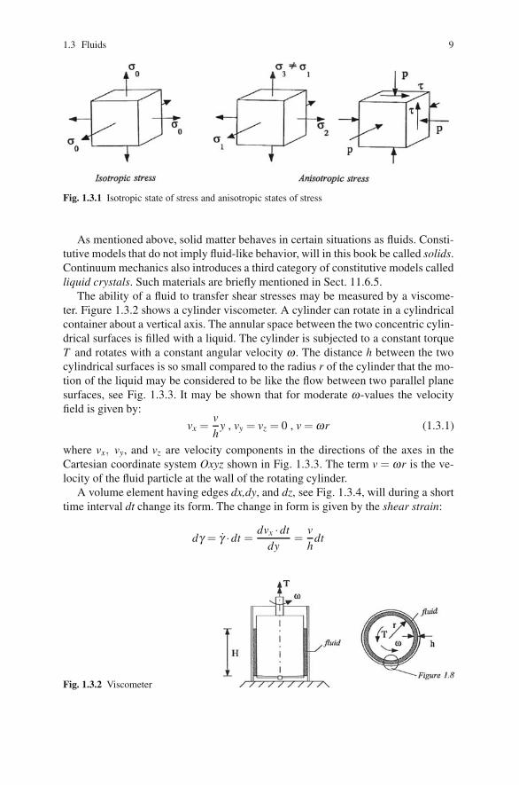
Figure 1.3.1 shows the difference of an isotropic state of stress and an anisotropicstate of stress. At an isotropic state of stress in a material point all material sur-faces through the point are subjected to the same normal stress, tension or com-pression, while tangential forces, i.e. shear stresses, on the surfaces are zero. At ananisotropic state of stress in a material point most material surfaces will experienceshear stresses.

1.3 Fluids 9

Fig. 1.3.1 Isotropic state of stress and anisotropic states of stress

As mentioned above, solid matter behaves in certain situations as fluids. Consti-tutive models that do not imply fluid-like behavior, will in this book be called solids.Continuum mechanics also introduces a third category of constitutive models calledliquid crystals. Such materials are briefly mentioned in Sect. 11.6.5.

The ability of a fluid to transfer shear stresses may be measured by a viscome-ter. Figure 1.3.2 shows a cylinder viscometer. A cylinder can rotate in a cylindricalcontainer about a vertical axis. The annular space between the two concentric cylin-drical surfaces is filled with a liquid. The cylinder is subjected to a constant torqueT and rotates with a constant angular velocity ω . The distance h between the twocylindrical surfaces is so small compared to the radius r of the cylinder that the mo-tion of the liquid may be considered to be like the flow between two parallel planesurfaces, see Fig. 1.3.3. It may be shown that for moderate ω-values the velocityfield is given by:

vx =vh

y , vy = vz = 0 , v = ωr (1.3.1)

where vx, vy, and vz are velocity components in the directions of the axes in theCartesian coordinate system Oxyz shown in Fig. 1.3.3. The term v = ωr is the ve-locity of the fluid particle at the wall of the rotating cylinder.

A volume element having edges dx,dy, and dz, see Fig. 1.3.4, will during a shorttime interval dt change its form. The change in form is given by the shear strain:

dγ = γ̇ ·dt =dvx ·dt

dy=

vh

dt

Fig. 1.3.2 Viscometer

10 1 Introduction

Fig. 1.3.3 Simple shear flow

The quantity:

γ̇ =vh

=rhω (1.3.2)

is called the rate of shear strain, or for short the shear rate. The flow described bythe velocity field (1.3.1) and illustrated in Fig. 1.3.3, is called simple shear flow.

The fluid element in Fig. 1.3.4 is subjected to normal stresses on all six sides andshear stresses on four sides, see Fig. 1.3.3. The normal stresses on the three pairs ofparallel sides may be different in a general case, but the shear stresses on the foursides are all equal. The shear stress τ may be determined from the law of balanceof angular momentum applied to the rotating cylinder. For the case of steady flowat constant angular velocity ω the torque T is balanced by the shear stress τ on thecylindrical wall. Thus:

(τ · r) · (2πr ·H) = T ⇒ τ =T

2πr2H(1.3.3)

The viscometer records the relationship between the torque T and the angular ve-locity ω . Using the formulas (1.3.2) and (1.3.3) we obtain a relationship betweenthe shear stress τ and the shear rate γ̇ .

A fluid is said to be purely viscous if the shear stress τ is a function of only γ̇ :

τ = τ (γ̇) (1.3.4)

An incompressible Newtonian fluid is a purely viscous fluid with a linear constitutiveequation:

τ = μγ̇ (1.3.5)

Fig. 1.3.4 Fluid element from Fig. 1.3.3

1.3 Fluids 11

Fig. 1.3.5 Purely viscous fluids

The coefficient μ is called the viscosity of the fluid and has the unit Ns/m2 = Pa.s,pascal-second. An alternative unit is poise [P]: 10P = 1 Pa.s. The viscosity variesstrongly with the temperature and to a certain extent also with the pressure in thefluid. For water at 0 ◦C μ = 1.8 · 10−3 Ns/m2 and at 20 ◦C μ = 1.0 · 10−3 Ns/m2.Usually a highly viscous fluid does not obey the linear law (1.3.5) and belongs to thenon-Newtonian fluids. However, some highly viscous fluids are Newtonian. Mixingglycerin and water gives a Newtonian fluid with viscosity varying from 1.0 · 10−3

to 1.5Ns/m2 at 20 ◦C, depending upon the concentration of glycerin. This fluid isoften used in tests comparing the behavior of a non-Newtonian fluid with that of aNewtonian fluid.

Figure 1.3.5 shows examples of the response of purely viscous non-Newtonianfluids. Most viscous non-Newtonian fluids are shear thinning fluids, sometimecalled pseudoplastic fluids. Examples are: nearly all polymer melts and polymersolutions, soap, biological fluids, and food products like mayonnaise. The expres-sion “shear thinning” is reflecting that “the apparent viscosity” τ/γ̇ decreases withincreasing shear rate. The expression “pseudoplastic” reflects the fact that the func-tion τ(γ̇) has similar characteristics as for viscoplastic fluids, see Fig. 1.3.6.

For a relatively small group of real liquids apparent viscosity τ/γ̇ increases withincreasing shear rate. These fluids are called shear-thickening fluids or dilatant flu-ids (expanding fluids). The last name reflects that these fluids often increase theirvolume when subjected to shear stresses.

Figure 1.3.6 shows the response of viscoplastic fluids. These material models arereally solids without appreciable deformation until the shear stress has reached a

Fig. 1.3.6 Viscoplastic fluids

12 1 Introduction

Fig. 1.3.7 Plug flow in a pipe

limit, called the yield shear stress τy. For shear stress τ > τy the materials behave asfluids. A Bingham fluid is a linearly viscous fluid when the shear stress τ > τy andthe constitutive equation for simple shear flow is:

τ =[τy

|γ̇| + μ]γ̇ for γ̇ �= 0 , |τ| ≤ τy for γ̇ = 0 (1.3.6)

The Bingham fluid is discussed in Sect. 10.11.2. Fluids with a yield shear stress are:mud, clay, drilling fluids, sand in water, margarine, tooth paste, some paints, andsome plastic melts.

A viscoplastic fluid in a pipe flow will obtain a velocity profile with a constantvelocity over an inner core, see Fig. 1.3.7. The core flows like a plug, giving thename plug flow for this phenomenon. Tooth paste flows as a plug flow when it issqueezed from the tube.

Chapter 8 Fluid Mechanics gives a presentation of classical fluid mechanicsfor inviscid fluids and Newtonian fluids. Non-Newtonian fluids are discussed inSects. 8.6 and 11.9.

1.4 Viscoelasticity

Propagation of sound in liquids and gases is an elastic response. Fluids are thereforein general both viscous and elastic, and the response is viscoelastic.

Figure 1.4.1 illustrates two phenomena that both are related to viscoelastic re-sponse in solid materials. Figure 1.4.1a shows the results of a creep test: A testspecimen is subjected to a constant axial force resulting in a constant normal stressσo over the cross-section of the specimen. The longitudinal strain in the axial direc-tion is recorded as a function of time. From the test diagram we see that the specimenmomentarily gets an initial strain ε i, which may be purely elastic or contain an elas-tic part ε i,e and a plastic part ε i,p. Under constant stress the strain increases withtime. This phenomenon is called creep. Creep may lead to fracture, partly becausethe material is weakening mechanically, and partly because the true stress over thecross-section of the specimen increases as the cross-sectional area decreases duringthe creep process. If the test specimen is unloaded abruptly at time t1, the elastic partε i,e of the initial strain disappears momentarily and is followed by a time dependentrestitution to ε = 0, or to a strain ε = ε p, which is a permanent or plastic strain.

1.4 Viscoelasticity 13

Fig. 1.4.1 Creep and stress relaxation

Figure 1.4.1b presents a stress relaxation test: A axial test specimen is sud-denly subjected to a constant longitudinal strain. The axial force, and thereby thecross-sectional normal stress, is recorded as a function of time. The stress decreasesasymptotically from the initial stress σ i towards a lower limit, the equilibrium stressσe, which may be zero.

Fig. 1.4.2 Viscoelastic mechanical models

14 1 Introduction

Materials, which under “normal” temperatures are responding purely elastically,may at higher, and sometimes lower, temperatures respond viscoelastically. For ex-ample, at temperatures above approximately 400 ◦C steel experiences creep andstress relaxation and thus has to be modelled as a viscoelastic material. Many plas-tics are viscoelastic at normal temperatures. Viscoelastic response is a dominatingproperty of these materials. Concrete also shows apparent viscoelastic properties.

Viscoelastic response may be illustrated using simple mechanical models con-sisting of elastic springs and viscous dampers, see Fig. 1.4.2. The models a)–d) areall meant to represent an axially loaded bar with a cross-sectional normal stress σand longitudinal strain ε in the axial direction.

A linearly elastic material, a Hookean solid, obeys Hooke’s law: σ = ηε .A linear helical spring, see Fig. 1.4.2a, is a mechanical model for a Hookean bar.A linearly viscous material is called a Newtonian material or a Newtonian fluid. Alinear damper, see Fig. 1.4.2b, is a mechanical model for a Newtonian bar and hasthe response equation:

σ = η̃ ε̇ (1.4.1)

where the viscosity η̃ is a material parameter, and ε̇ ≡ dε/dt is the strain rate.For uniaxial stress the Maxwell fluid is defined by the response equation:

ση̃

+σ̇η

= ε̇ (1.4.2)

and named after James Clerk Maxwell [1831–1879]. A linear damper and spring inseries, see Fig. 1.4.2c, is a mechanical model for a Maxwell bar. Equation (1.4.2)is a result of adding the strain rates σ/η̃ for the damper and σ̇/η for the spring.Figure 1.4.3 shows how this material model responds in creep and relaxation tests.

For uniaxial stress the Kelvin solid is defined by the response equation:

σ = ηε+ η̃ε̇ (1.4.3)

and named after Lord Kelvin (William Thompson) [1824–1907]. A spring anddamper in parallel, see Fig. 1.4.2d, is a mechanical model of a Kelvin bar. Equa-

Fig. 1.4.3 Creep and relaxation tests of a Maxwell bar