continuous time markov chain models for chemical reaction networks
TRANSCRIPT

Chapter 1
CONTINUOUS TIME MARKOV CHAIN MODELSFOR CHEMICAL REACTION NETWORKS
David F. Anderson ∗
Departments of MathematicsUniversity of Wisconsin - Madison480 Lincoln DriveMadison, WI 53706-1388http://www.math.wisc.edu/∼[email protected]
Thomas G. Kurtz, †
Departments of Mathematics and StatisticsUniversity of Wisconsin - Madison480 Lincoln DriveMadison, WI 53706-1388http://www.math.wisc.edu/∼[email protected]
Abstract A reaction network is a chemical system involving multiple reactionsand chemical species. The simplest stochastic models of such networkstreat the system as a continuous time Markov chain with the state beingthe number of molecules of each species and with reactions modeled aspossible transitions of the chain. This chapter is devoted to the mathe-matical study of such stochastic models. We begin by developing muchof the mathematical machinery we need to describe the stochastic mod-els we are most interested in. We show how one can represent countingprocesses of the type we need in terms of Poisson processes. This randomtime-change representation gives a stochastic equation for continuous-time Markov chain models. We include a discussion on the relation-ship between this stochastic equation and the corresponding martingaleproblem and Kolmogorov forward (master) equation. Next, we exploit
∗Research supported in part by NSF grant DMS 05-53687†Research supported in part by NSF grants DMS 05-53687 and DMS 08-05793
2
the representation of the stochastic equation for chemical reaction net-works and, under what we will refer to as the classical scaling, showhow to derive the deterministic law of mass action from the Markovchain model. We also review the diffusion, or Langevin, approximation,include a discussion of first order reaction networks, and present a largeclass of networks, those that are weakly reversible and have a deficiencyof zero, that induce product-form stationary distributions. Finally, wediscuss models in which the numbers of molecules and/or the reactionrate constants of the system vary over several orders of magnitude. Weshow that one consequence of this wide variation in scales is that differ-ent subsystems may evolve on different time scales and this time-scalevariation can be exploited to identify reduced models that capture thebehavior of parts of the system. We will discuss systematic ways ofidentifying the different time scales and deriving the reduced models.
Keywords: Reaction network, Markov chain, law of mass action, law of large num-bers, central limit theorem, diffusion approximation, Langevin approx-imation, stochastic equations, multiscale analysis, stationary distribu-tions
MSC 2010: 60J27, 60J28, 60J80, 60F17, 80A30, 92C40
1. IntroductionThe idea of modeling chemical reactions as a stochastic process at
the molecular level dates back at least to [12] with a rapid developmentbeginning in the 1950s and 1960s. (See, for example, [6, 7, 39].) For thereaction
A+B ⇀ C
in which one molecule of A and one molecule of B are consumed toproduce one molecule of C, the intuition for the model for the reactionis that the probability of the reaction occurring in a small time inter-val (t, t + ∆t] should be proportional to the product of the numbers ofmolecules of each of the reactants and to the length of the time interval.In other words, since for the reaction to occur a molecule of A and amolecule of B must be close to each other, the probability should beproportional to the number of pairs of molecules that can react. A moresystematic approach to this conclusion might be to consider the follow-ing probability problem: Suppose k red balls (molecules of A) and lblack balls (molecules of B) are placed uniformly at random in n boxes,where n is much larger than k and l. What is the probability that atleast one red ball ends up in the same box as a black ball? We leave it
Continuous time Markov chain models for chemical reaction networks 3
to the reader to figure that out. For a more physically based argument,see [22].
Our more immediate concern is that the calculation, however justi-fied, assumes that the numbers of molecules of the chemical species areknown. That assumption means that what is to be computed is a con-ditional probability, that is, a computation that uses information thatmight not (or could not) have been known when the experiment wasfirst set up.
Assuming that at time t there are XA(t) molecules of A and XB(t)molecules of B in our system, we express our assumption about theprobability of the reaction occurring by
P{reaction occurs in (t, t+ ∆t]|Ft} ≈ κXA(t)XB(t)∆t (1.1)
where Ft represents the information about the system that is availableat time t and κ is a positive constant, the reaction rate constant. SinceKolmogorov’s fundamental work [29], probabilists have modeled infor-mation as a σ-algebra (a collection of sets with particular properties)of events (subsets of possible outcomes) in the sample space (the set ofall possible outcomes). Consequently, mathematically, Ft is a σ-algebra,but readers unfamiliar with this terminology should just keep the ideaof information in mind when we write expressions like this, that is, Ftjust represents the information available at time t.
One of our first goals will be to show how to make the intuitive as-sumption in (1.1) into a precise mathematical model. Our model willbe formulated in terms of XA, XB, and XC which will be stochas-tic processes, that is, random functions of time. The triple X(t) =(XA(t), XB(t), XC(t)) gives the state of the process at time t. Simplebookkeeping implies
X(t) = X(0) +R(t)
−1−11
, (1.2)
where R(t) is the number of times the reaction has occurred by time tand X(0) is the vector giving the numbers of molecules of each of thechemical species in the system at time zero. We will assume that tworeactions cannot occur at exactly the same time, so R is a countingprocess, that is, R(0) = 0 and R is constant except for jumps of plusone.
Our first task, in Section 2, will be to show how one can representcounting processes of the type we need in terms of the most elemen-tary counting process, namely, the Poisson process. Implicit in the factthat the right side of (1.1) depends only on the current values of XA
4
and XB is the assumption that the model satisfies the Markov property,that is, the future of the process only depends on the current value, noton values at earlier times. The representation of counting processes interms of Poisson processes then gives a stochastic equation for a generalcontinuous-time Markov chain. There are, of course, other ways of spec-ifying a continuous-time Markov chain model, and Section 2 includes adiscussion of the relationship between the stochastic equation and thecorresponding martingale problem and Kolmogorov forward (master)equation. We also include a brief description of the common methods ofsimulating the models.
Exploiting the representation as a solution of a stochastic equation, inSection 3 we discuss stochastic models for chemical reaction networks.Under what we will refer to as the classical scaling, we show how to de-rive the deterministic law of mass action from the Markov chain modeland introduce the diffusion or Langevin approximation. We also discussthe simple class of networks in which all reactions are unary and indicatehow the large literature on branching processes and queueing networksprovides useful information about this class of networks. Many of thesenetworks have what is known in the queueing literature as product formstationary distributions, which makes the stationary distributions easyto compute. The class of networks that have stationary distributions ofthis form is not restricted to unary networks, however. In particular,all networks that satisfy the conditions of the zero-deficiency theoremof Feinberg [16, 17], well-known in deterministic reaction network the-ory, have product-form stationary distributions. There is also a briefdiscussion of models of reaction networks with delays.
The biological systems that motivate the current discussion may in-volve reaction networks in which the numbers of molecules of the chem-ical species present in the system vary over several orders of magnitude.The reaction rates may also vary widely. One consequence of this widevariation in scales is that different subsystems may evolve on differenttime scales and this time-scale variation can be exploited to identify re-duced models that capture the behavior of parts of the system. Section4 discusses systematic ways of identifying the different time scales andderiving the reduced models.
Although much of the discussion that follows is informal and is in-tended to motivate rather than rigorously demonstrate the ideas andmethods we present, any lemma or theorem explicitly identified as suchis rigorously justifiable, or at least we intend that to be the case. Ourintention is to prepare an extended version of this paper that includesdetailed proofs of most or all of the theorems included.

Continuous time Markov chain models for chemical reaction networks 5
2. Counting processes and continuous timeMarkov chains
The simplest counting process is a Poisson process, and Poisson pro-cesses will be the basic building blocks that we use to obtain more com-plex models.
2.1 Poisson processesA Poisson process is a model for a series of random observations oc-
curring in time.
x x x x x x x x
t
Let Y (t) denote the number of observations by time t. In the figureabove, Y (t) = 6. Note that for t < s, Y (s)− Y (t) is the number of ob-servations in the time interval (t, s]. We make the following assumptionsabout the model.
1) Observations occur one at a time.
2) Numbers of observations in disjoint time intervals are independentrandom variables, i.e., if t0 < t1 < · · · < tm, then Y (tk)− Y (tk−1),k = 1, . . . ,m are independent random variables.
3) The distribution of Y (t+ a)− Y (t) does not depend on t.
The following result can be found in many elementary books on prob-ability and stochastic processes. See, for example, Ross [41].
Theorem 1.1 Under assumptions 1), 2), and 3), there is a constantλ > 0 such that, for t < s, Y (s) − Y (t) is Poisson distributed withparameter λ(s− t), that is,
P{Y (s)− Y (t) = k} =(λ(s− t))k
k!e−λ(s−t). (2.1)
If λ = 1, then Y is a unit (or rate one) Poisson process. If Y is a unitPoisson process and Yλ(t) ≡ Y (λt), then Yλ is a Poisson process withparameter λ. Suppose Yλ(t) = Y (λt) and Ft represents the informationobtained by observing Yλ(s), for s ≤ t. Then by the independenceassumption and (2.1)
P{Yλ(t+ ∆t)− Yλ(t) > 0|Ft} = P{Yλ(t+ ∆t)− Yλ(t) > 0}= 1− e−λ∆t ≈ λ∆t. (2.2)
6
The following facts about Poisson processes play a significant role inour analysis of the models we will discuss.
Theorem 1.2 If Y is a unit Poisson process, then for each u0 > 0,
limn→∞
supu≤u0
|Y (nu)n
− u| = 0 a.s.
Proof. For fixed u, by the independent increments assumption, theresult is just the ordinary law of large numbers. The uniformity followsby monotonicity. �
The classical central limit theorem implies
limn→∞
P{Y (nu)− nu√n
≤ x} =∫ x
−∞
1√2πe−y
2/2dy = P{W (u) ≤ x},
where W is a standard Brownian motion. In fact, the approximation isuniform on bounded time intervals in much the same sense that the limitin Theorem 1.2 is uniform. This result is essentially Donsker’s functionalcentral limit theorem [13]. It suggests that for large n
Y (nu)− nu√n
≈W (u),Y (nu)n
≈ u+1√nW (u)
where the approximation is uniform on bounded time intervals. One wayto make this approximation precise is through the strong approximationtheorem of Komlos, Major, and Tusnady [30, 31], which implies thefollowing.
Lemma 1.3 A unit Poisson process Y and a standard Brownian motionW can be constructed so that
Γ ≡ supt≥0
|Y (t)− t−W (t)|log(2 ∨ t)
<∞ a.s.
and there exists c > 0 such that E[ecΓ] <∞.
Proof. See Corollary 7.5.5 of [15]. �
Note that ∣∣∣∣Y (nt)− nt√n
− 1√nW (nt)
∣∣∣∣ ≤ log(nt ∨ 2)√n
Γ, (2.3)
and that 1√nW (nt) is a standard Brownian motion.

Continuous time Markov chain models for chemical reaction networks 7
2.2 Continuous time Markov chainsThe calculation in (2.2) and the time-change representation Yλ(t) =
Y (λt) suggest the possibility of writing R in (1.2) as
R(t) = Y (∫ t
0κXA(s)XB(s)ds)
and hence XA(t)XB(t)XC(t)
≡ X(t) = X(0) +
−1−11
Y (∫ t
0κXA(s)XB(s)ds). (2.4)
Given Y and the initial state X(0) (which we assume is independent ofY ), (2.4) is an equation that uniquely determines X for all t > 0. To seethat this assertion is correct, let τk be the kth jump time of Y . Thenletting
ζ =
−1−11
,
(2.4) implies X(t) = X(0) for 0 ≤ t < τ1, X(t) = X(0) + ζ for τ1 ≤t < τ2, and so forth. To see that the solution of this equation has theproperties suggested by (1.1), let λ(X(t)) = κXA(t)XB(t) and observethat occurrence of the reaction in (t, t+ ∆t] is equivalent to R(t+ ∆t) >R(t), so the left side of (1.1) becomes
P{R(t+ ∆t) > R(t)|Ft}= 1− P{R(t+ ∆t) = R(t)|Ft}
= 1− P{Y (∫ t
0λ(X(s))ds+ λ(X(t))∆t) = Y (
∫ t
0λ(X(s))ds)|Ft}
= 1− e−λ(X(t))∆t ≈ λ(X(t))∆t,
where the third equality follows from the fact that Y (∫ t
0 λ(X(s))ds) andX(t) are part of the information in Ft (are Ft-measurable in the math-ematical terminology) and the independence properties of Y .
More generally, a continuous time Markov chain X taking values inZd is specified by giving its transition intensities (propensities in muchof the chemical physics literature) λl that determine
P{X(t+ ∆t)−X(t) = ζl|FXt } ≈ λl(X(t))∆t, (2.5)
for the different possible jumps ζl ∈ Zd, where FXt is the σ−algebragenerated by X (all the information available from the observation of
8
the process up to time t). If we write
X(t) = X(0) +∑l
ζlRl(t)
where Rl(t) is the number of jumps of ζl at or before time t, then (2.5)implies
P{Rl(t+ ∆t)−Rl(t) = 1|FXt } ≈ λl(X(t))∆t, l ∈ Zd.
Rl is a counting process with intensity λl(X(t)), and by analogy with(2.4), we write
X(t) = X(0) +∑
ζlYl(∫ t
0λl(X(s))ds), (2.6)
where the Yl are independent unit Poisson processes. This equationhas a unique solution by the same jump by jump argument used aboveprovided
∑l λl(x) <∞ for all x. Unless we add additional assumptions,
we cannot rule out the possibility that the solution only exists up to somefinite time. For example, if d = 1 and λ1(k) = (1 + k)2, the solution of
X(t) = Y1(∫ t
0(1 +X(s))2ds)
hits infinity in finite time. To see why this is the case, compare theabove equation to the ordinary differential equation
x(t) = (1 + x(t))2, x(0) = 0.
2.3 Equivalence of stochastic equations andmartingale problems
There are many ways of relating the intensities λl to the stochasticprocess X, and we will review some of these in later sections, but thestochastic equation (2.6) has the advantage of being intuitive (λl has anatural interpretation as a “rate”) and easily generalized to take intoaccount such properties as external noise, in which (2.6) becomes
X(t) = X(0) +∑
ζlYl(∫ t
0λl(X(s), Z(s))ds)
where Z is a stochastic process independent ofX(0) and the Yl, or delays,in which (2.6) becomes
X(t) = X(0) +∑
ζlYl(∫ t
0λl(X(s), X(s− δ))ds),
Continuous time Markov chain models for chemical reaction networks 9
or perhaps the λl become even more complicated functions of the pastof X. We will also see that these stochastic equations let us exploit well-known properties of the Poisson processes Yl to study the properties ofX.
The basic building blocks of our models remain the counting processesRl and their intensities expressed as functions of the past of the Rland possibly some additional stochastic input independent of the Yl (forexample, the initial condition X(0) or the environmental noise Z).
For the moment, we focus on a finite system of counting processesR = (R1, . . . , Rm) given as the solution of a system of equations
Rl(t) = Yl(∫ t
0γl(s,R)ds), (2.7)
where the γl are nonanticipating in the sense that
γl(t, R) = γl(t, R(· ∧ t)), t ≥ 0,
that is, at time t, γl(t, R) depends only on the past of R up to time t,and the Yl are independent, unit Poisson processes. The independenceof the Yl ensures that only one of the Rl jumps at a time. Let τk bethe kth jump time of R. Then any system of this form has the propertythat for all l and k,
Mkl (t) ≡ Rl(t ∧ τk)−
∫ t∧τk
0γl(s,R)ds
is a martingale, that is, there exists a filtration {Ft} such that
E[Mkl (t+ s)|Ft] = Mk
l (t), t, s ≥ 0.
Note that
limk→∞
E[Rl(t ∧ τk)] = limk→∞
E[∫ t∧τk
0γl(s,R)ds],
allowing ∞ = ∞, and if the limit is finite for all l and t, then τ∞ = ∞and for each l,
Ml(t) = Rl(t)−∫ t
0γl(s,R)ds
is a martingale.There is a converse to these assertions. If (R1, . . . , Rm) are counting
processes adapted to a filtration {Ft} and (λ1, . . . , λm) are nonnegativestochastic processes adapted to {Ft} such that for each k and l,
Rl(t ∧ τk)−∫ t∧τk
0λl(s)ds
10
is a {Ft}-martingale, we say that λl is the {Ft}-intensity for Rl.
Lemma 1.4 Assume that R = (R1, . . . , Rm) is a system of countingprocesses with no common jumps and λl is the {Ft}-intensity for Rl.Then there exist independent unit Poisson processes Y1, . . . , Ym (perhapson an enlarged sample space) such that
Rl(t) = Yl(∫ t
0λl(s)ds).
Proof. See Meyer [40] and Kurtz [36]. �
This lemma suggests the following alternative approach to relatingthe intensity of a counting process to the corresponding counting pro-cess. Again, given nonnegative, nonanticipating functions γl, the intu-itive problem is to find counting processes Rl such that
P{Rl(t+ ∆t) > Rl(t)|Ft} ≈ γl(t, R)∆t,
which we now translate into the following martingale problem. In thefollowing definition Jm[0,∞) denotes the set of m−dimensional cadlag(right continuous with left limits at each t > 0) counting paths.
Definition 1.5 Let γl, l = 1, . . . ,m, be nonnegative, nonanticipatingfunctions defined on Jm[0,∞). Then a family of counting processes R =(R1, . . . , Rm) is a solution of the martingale problem for (γ1, . . . , γm)if the Rl have no simultaneous jumps and there exists a filtration {Ft}such that R is adapted to {Ft} and for each l and k,
Rl(t ∧ τk)−∫ t∧τk
0γl(s,R)ds
is a {Ft}-martingale.
Of course, the solution of (2.7) is a solution of the martingale problemand Lemma 1.4 implies that every solution of the martingale problemcan be written as a solution of the stochastic equation. Consequently,the stochastic equation and the martingale problem are equivalent waysof specifying the system of counting processes that corresponds to the γl.The fact that the martingale problem uniquely characterizes the systemof counting processes is a special case of a theorem of Jacod [24].
2.4 Thinning of counting processesConsider a single counting process R0 with {Ft}-intensity λ0, and let
p(t, R0) be a cadlag, nonanticipating function with values in [0, 1]. For
Continuous time Markov chain models for chemical reaction networks 11
simplicity, assume
E[R0(t)] = E[∫ t
0λ0(s)ds] <∞.
We want to construct a new counting process R1 such that at eachjump of R0, R1 jumps with probability p(t−, R0). Perhaps the simplestconstruction is to let ξ0, ξ1, . . . be independent, uniform [0, 1] randomvariables that are independent of R0 and to define
R1(t) =∫ t
01[0,p(s−,R0)](ξR0(s−))dR0(s).
Since with probability one,
R1(t) = limn→∞
bntc∑k=0
1[0,p( kn,R0)](ξR0( k
n))(R0(
k + 1n
)−R0(k
n)),
where bzc is the integer part of z, setting R0(t) = R0(t)−∫ t
0 λ0(s)ds, wesee that
R1(t)−∫ t
0λ0(s)p(s,R0)ds
=∫ t
0(1[0,p(s−,R0)](ξR0(s−))− p(s−, R0))dR0(s)
+∫ t
0p(s−, R0)dR0(s)
is a martingale (because both terms on the right are martingales). Hence,R1 is a counting process with intensity λ0(t)p(t, R0). We could alsodefine
R2(t) =∫ t
01(p(s−,R0),1](ξR0(s−))dR0(s),
so that R1 and R2 would be counting processes without simultaneousjumps having intensities λ0(t)p(t, R0) and λ0(t)(1− p(t, R0)).
Note that we could let p be a nonanticipating function of both R0
and R1, or equivalently, R1 and R2. With that observation in mind, letγ0(t, R) be a nonnegative, nonanticipating function of R = (R1, . . . , Rm),and let pl(t, R), l = 1, . . . ,m, be cadlag nonnegative, nonanticipatingfunctions satisfying
∑ml=1 pl(t, R) ≡ 1. Let Y be a unit Poisson process
and ξ0, ξ1, . . . be independent, uniform [0, 1] random variables that areindependent of Y , and set q0 = 0 and for 1 ≤ l ≤ m set ql(t, R) =

12∑li=1 pi(t, R). Now consider the system
R0(t) = Y (∫ t
0γ0(s,R)ds) (2.8)
Rl(t) =∫ t
01(ql−1(s−,R),ql(s−,R)](ξR0(s−))dR0(s). (2.9)
Then R = (R1, . . . , Rm) is a system of counting processes with intensitiesλl(t) = γ0(t, R)pl(t, R).
If, as in the time-change equation (2.7) and the equivalent martingaleproblem described in Definition 1.5, we start with intensities γ1, . . . , γm,we can define
γ0(t, R) =m∑l=1
γl(t, R), pl(t, R) =γl(t, R)γ0(t, R)
,
and the solution of the system (2.8) and (2.9) will give a system ofcounting processes with the same distribution as the solution of the time-change equation or the martingale problem. Specializing to continuous-time Markov chains and defining
λ0(x) =∑l
λl(x), ql(x) =l∑
i=1
λi(x)/λ0(x),
the equations become
R0(t) = Y (∫ t
0λ0(X(s))ds) (2.10)
X(t) = X(0) +∑l
ζl
∫ t
01(ql−1(X(s−)),ql(X(s−)](ξR0(s−))dR0(s).
This representation is commonly used for simulation, see section 2.6.
2.5 The martingale problem and forwardequation for Markov chains
Let X satisfy (2.6), and for simplicity, assume that τ∞ = ∞, thatonly finitely many of the λl are not identically zero, and that
E[Rl(t)] = E[∫ t
0λl(X(s))ds] <∞, l = 1, . . . ,m.
Then for f a bounded function on Zd,
f(X(t)) = f(X(0)) +∑l
∫ t
0(f(X(s−) + ζl)− f(X(s−)))dRl(t)
Continuous time Markov chain models for chemical reaction networks 13
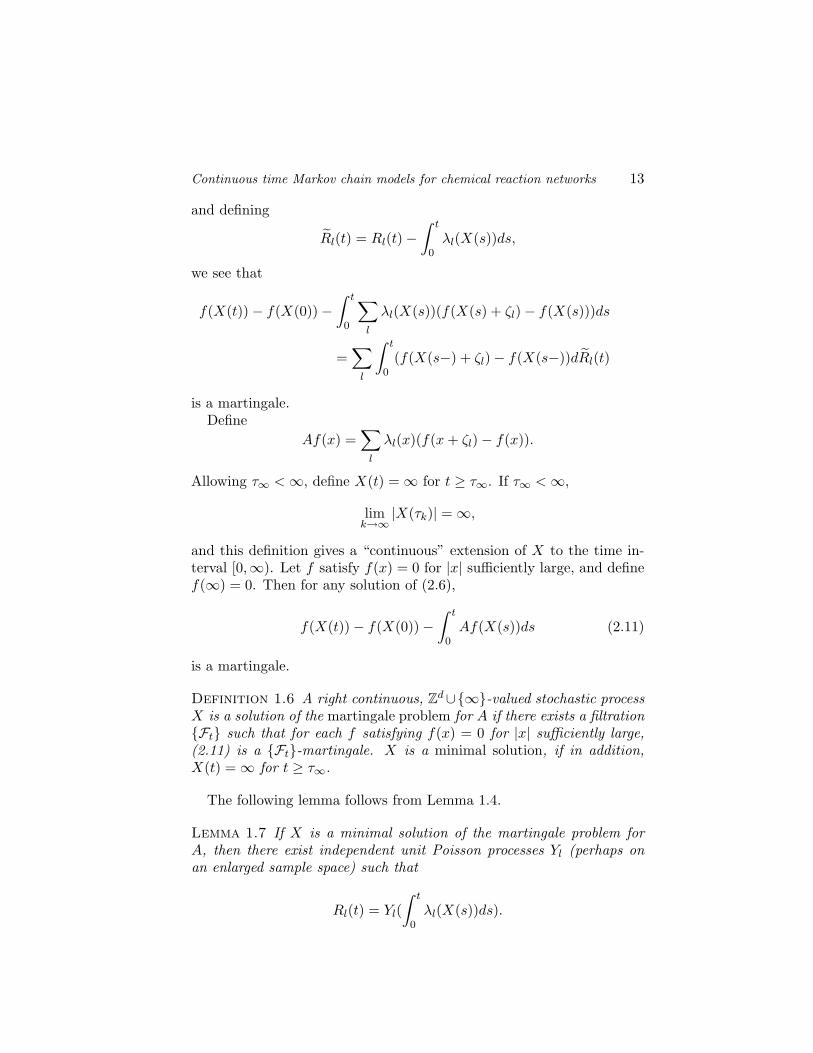
and defining
Rl(t) = Rl(t)−∫ t
0λl(X(s))ds,
we see that
f(X(t))− f(X(0))−∫ t
0
∑l
λl(X(s))(f(X(s) + ζl)− f(X(s)))ds
=∑l
∫ t
0(f(X(s−) + ζl)− f(X(s−))dRl(t)
is a martingale.Define
Af(x) =∑l
λl(x)(f(x+ ζl)− f(x)).
Allowing τ∞ <∞, define X(t) =∞ for t ≥ τ∞. If τ∞ <∞,
limk→∞
|X(τk)| =∞,
and this definition gives a “continuous” extension of X to the time in-terval [0,∞). Let f satisfy f(x) = 0 for |x| sufficiently large, and definef(∞) = 0. Then for any solution of (2.6),
f(X(t))− f(X(0))−∫ t
0Af(X(s))ds (2.11)
is a martingale.
Definition 1.6 A right continuous, Zd∪{∞}-valued stochastic processX is a solution of the martingale problem for A if there exists a filtration{Ft} such that for each f satisfying f(x) = 0 for |x| sufficiently large,(2.11) is a {Ft}-martingale. X is a minimal solution, if in addition,X(t) =∞ for t ≥ τ∞.
The following lemma follows from Lemma 1.4.
Lemma 1.7 If X is a minimal solution of the martingale problem forA, then there exist independent unit Poisson processes Yl (perhaps onan enlarged sample space) such that
Rl(t) = Yl(∫ t
0λl(X(s))ds).
14
The martingale property implies
E[f(X(t))] = E[f(X(0))] +∫ t
0E[Af(X(s))]ds
and taking f(x) = 1{y}(x), we have
P{X(t) = y} = P{X(0) = y}+∫ t
0(∑l
λl(y − ζl)P{X(s) = y − ζl}
−∑l
λl(y)P{X(s) = y})ds
giving the Kolmogorov forward or master equation for the distribution ofX. In particular, defining py(t) = P{X(t) = y} and νy = P{X(0) = y},{py} satisfies the system of differential equations
py(t) =∑l
λl(y − ζl)py−ζl(t)− (∑l
λl(y))py(t), (2.12)
with initial condition py(0) = νy.
Lemma 1.8 Let {νy} be a probability distribution on Zd, and let X(0)satisfy P{X(0) = y} = νy. The system of differential equations (2.12)has a unique solution satisfying py(0) = νy and
∑y py(t) ≡ 1 if and only
if the solution of (2.6) satisfies τ∞ =∞.
2.6 SimulationThe stochastic equations (2.6) and (2.10) suggest methods of simulat-
ing continuous-time Markov chains, and these methods are, in fact, wellknown. Equation (2.6) corresponds to the next reaction (next jump)method as defined by Gibson and Bruck [19].
The algorithm obtained by simulating (2.10) is known variously asthe embedded chain method or Gillespie’s [20, 21] direct method or thestochastic simulation algorithm (SSA).
If we define an Euler-type approximation for (2.6), that is, for 0 =τ0 < τ1 < · · · , recursively define
X(τn) = X(0) +∑l
ζlYl
(n−1∑k=0
λl(X(τk))(τk+1 − τk)
),
we obtain Gillespie’s [23] τ -leap method.
Continuous time Markov chain models for chemical reaction networks 15
2.7 Stationary distributionsWe restrict our attention to continuous-time Markov chains for which
τ∞ = ∞ for all initial values and hence, given X(0), the process isuniquely determined as a solution of (2.6), (2.10), or the martingaleproblem given by Definition 1.6, and the one-dimensional distributionsare uniquely determined by (2.12). A probability distribution π is calleda stationary distribution for the Markov chain if X(0) having distri-bution π implies X is a stationary process, that is, for each choice of0 ≤ t1 < · · · < tk, the joint distribution of
(X(t+ t1), . . . , X(t+ tk))
does not depend on t.If X(0) has distribution π, then since E[f(X(0))] = E[f(X(t))] =∑x f(x)π(x), the martingale property for (2.11) implies
0 = E[∫ t
0Af(X(s))ds] = t
∑x
Af(x)π(x),
and as in the derivation of (2.12),∑l
λl(y − ζl)π(y − ζl)− (∑l
λl(y))π(y) = 0.
3. Reaction networksWe consider a network of r0 chemical reactions involving s0 chemical
species, S1, . . . , Ss0 ,
s0∑i=1
νikSi ⇀
s0∑i=1
ν ′ikSi, k = 1, . . . , r0,
where the νik and ν ′ik are nonnegative integers. Let the componentsof X(t) give the numbers of molecules of each species in the system attime t. Let νk be the vector whose ith component is νik, the number ofmolecules of the ith chemical species consumed in the kth reaction, andlet ν ′k be the vector whose ith component is ν ′ik, the number of moleculesof the ith species produced by the kth reaction. Let λk(x) be the rate atwhich the kth reaction occurs, that is, it gives the propensity/intensityof the kth reaction as a function of the numbers of molecules of thechemical species.
If the kth reaction occurs at time t, the new state becomes
X(t) = X(t−) + ν ′k − νk.
16
The number of times that the kth reaction occurs by time t is given bythe counting process satisfying
Rk(t) = Yk(∫ t
0λk(X(s))ds),
where the Yk are independent unit Poisson processes. The state of thesystem then satisfies
X(t) = X(0) +∑k
Rk(t)(ν ′k − νk)
= X(0) +∑k
Yk(∫ t
0λk(X(s))ds)(ν ′k − νk).
To simplify notation, we will write
ζk = ν ′k − νk.
3.1 Rates for the law of mass actionThe stochastic form of the law of mass action says that the rate at
which a reaction occurs should be proportional to the number of distinctsubsets of the molecules present that can form the inputs for the reaction.Intuitively, the mass action assumption reflects the idea that the systemis well-stirred in the sense that all molecules are equally likely to be atany location at any time. For example, for a binary reaction S1+S2 ⇀ S3
or S1 + S2 ⇀ S3 + S4,λk(x) = κkx1x2,
where κk is a rate constant. For a unary reaction S1 ⇀ S2 or S1 ⇀S2 + S3, λk(x) = κkx1. For 2S1 ⇀ S2, λk(x) = κkx1(x1 − 1).
For a binary reaction S1 + S2 ⇀ S3, the rate should vary inverselywith volume, so it would be better to write
λNk (x) = κkN−1x1x2 = Nκkz1z2,
where classically, N is taken to be the volume of the system times Avo-gadro’s number and zi = N−1xi is the concentration in moles per unitvolume. For 2S1 → S2, since N is very large,
1Nκkx1(x1 − 1) = Nκkz1(z1 −
1N
) ≈ Nκkz21 .
Note that unary reaction rates also satisfy
λk(x) = κkxi = Nκkzi.

Continuous time Markov chain models for chemical reaction networks 17
Although, reactions of order higher than binary may not be physical,if they were, the analogous form for the intensity would be
λNk (x) = κk
∏i νik!
N |νk|−1
∏i
(xiνik
)= Nκk
∏i νik!N |νk|
∏(xiνik
),
where |νk| =∑
i νik. Again z = N−1x gives the concentrations in molesper unit volume, and
λNk (x) ≈ Nκk∏i
zνiki ≡ Nλk(z), (3.1)
where λk is the usual deterministic form of mass action kinetics.
3.2 General form for the classical scalingSetting CN (t) = N−1X(t) and using (3.1)
CN (t) = CN (0) +∑k
N−1Yk(∫ t
0λNk (X(s))ds)ζk
≈ CN (0) +∑k
N−1Yk(N∫ t
0λk(CN (s))ds)ζk
= CN (0) +∑k
N−1Yk(N∫ t
0λk(CN (s))ds)ζk +
∫ t
0F (CN (s))ds,
where Yk(u) = Yk(u)− u is the centered process and
F (z) ≡∑k
κk∏i
zνiki ζk.
The law of large numbers for the Poisson process, Lemma 1.2, impliesN−1Y (Nu) ≈ 0, so
CN (t) ≈ CN (0)+∑k
∫ t
0κk∏i
CNi (s)νikζkds = CN (0)+∫ t
0F (CN (s))ds,
which in the limit as N → ∞ gives the classical deterministic law ofmass action
C(t) =∑k
κk∏i
Ci(t)νikζk = F (C(t)). (3.2)
(See [32, 34, 35] for precise statements about this limit.)Since by (2.3),
1√NYk(Nu) =
Yk(Nu)−Nu√N
18
is approximately a Brownian motion,
V N (t) ≡√N(CN (t)− C(t))
≈ V N (0) +√N(∑k
1NYk(N
∫ t
0λk(CN (s))ds)ζk −
∫ t
0F (C(s))ds)
= V N (0) +∑k
1√NYk(N
∫ t
0λk(CN (s))ds)ζk
+∫ t
0
√N(F (CN (s))− F (C(s)))ds
≈ V N (0) +∑k
Wk(∫ t
0λk(C(s))ds)ζk +
∫ t
0∇F (C(s))V N (s)ds,
where the second approximation follows from (3.1). The limit as N goesto infinity gives V N ⇒ V where
V (t) = V (0) +∑k
Wk(∫ t
0λk(C(s))ds)ζk +
∫ t
0∇F (C(s))V (s)ds. (3.3)
(See [33, 35, 42] and Chapter 11 of [15].) This limit suggests the approx-imation
CN (t) ≈ CN (t) ≡ C(t) +1√NV (t). (3.4)
Since (3.3) is a linear equation driven by a Gaussian process, V is Gaus-sian as is CN .
3.3 Diffusion/Langevin approximationsThe first steps in the argument in the previous section suggest simply
replacing the rescaled centered Poisson processes 1√NYk(N ·) by indepen-
dent Brownian motions and considering a solution of
DN (t) = DN (0) +∑k
1√NWk(
∫ t
0λk(DN (s))ds)ζk +
∫ t
0F (DN (s))ds
(3.5)as a possible approximation for CN . Unfortunately, even though onlyordinary integrals appear in this equation, the theory of the equation isnot quite as simple as it looks. Unlike (2.6) where uniqueness of solutionsis immediate, no general uniqueness theorem is known for (3.5) withoutan additional requirement on the solution. In particular, setting
τNk (t) =∫ t
0λk(DN (s))ds,

Continuous time Markov chain models for chemical reaction networks 19
we must require that the solution DN is compatible with the Brownianmotions Wk in the sense that Wk(τNk (t)+u)−Wk(τNk (t)) is independentof FDNt for all k, t ≥ 0, and u ≥ 0. This requirement is intuitivelynatural and is analogous to the requirement that a solution of an Itoequation be nonanticipating. In fact, we have the following relationshipbetween (3.5) and a corresponding Ito equation.
Lemma 1.9 If DN is a compatible solution of (3.5), then there existindependent standard Brownian motions Bk (perhaps on an enlargedsample space) such that DN is a solution of the Ito equation
DN (t) = DN (0) +∑k
1√N
∫ t
0
√λ(DN (s)dBk(s)ζk +
∫ t
0F (DN (s))ds.
(3.6)
Proof. See [35, 36] and Chapter 11 of [15]. For a general discussion ofcompatibility, see [37], in particular, Example 3.20. �
In the chemical physics literature, DN is known as the Langevin ap-proximation for the continuous-time Markov chain model determinedby the master equation. Just as there are alternative ways of deter-mining the continuous-time Markov chain model, there are alternativeapproaches to deriving the Langevin approximation. For example, CN
is a solution of the martingale problem corresponding to
ANf(x) =∑k
Nλk(x)(f(x+N−1ζk)− f(x)),
and if f is three times continuously differentiable with compact support,
ANf(x) = LNf(x) +O(N−2),
whereLNf(x) =
12N
∑k
ζ>k ∂2f(x)ζ>k + F (x) · ∇f(x),
and any compatible solution of (3.5) is a solution of the martingaleproblem for LN , that is, there is a filtration {FNt } such that
f(DN (t))− f(DN (0))−∫ t
0LNf(DN (s))ds
is a {FNt }-martingale for each twice continuously differentiable functionhaving compact support. The converse also holds, that is, any solution
20
of the martingale problem for LN that does not hit infinity in finite timecan be obtained as a compatible solution of (3.5) or equivalently, as asolution of (3.6).
Finally, the Langevin approximation can be derived starting with themaster equation. First rewrite (2.12) as
pN (y, t) =∑l
Nλl(y −N−1ζl)pN (y −N−1ζl, t)− (∑l
Nλl(y))pN (y, t),
(3.7)where now
pN (y, t) = P{CN (t) = y}.
Expanding λl(y−N−1ζl)pN (y−N−1ζl) in a Taylor series (the Kramer-Moyal expansion, or in this context, the system-size expansion of vanKampen; see [42]) and discarding higher order terms gives
pN (y, t) ≈ 12N
∑l
ζ>l ∂2(λl(y)pN (y, t))ζk −
∑l
ζl · ∇(λl(y)pN (y, t)).
Replacing ≈ by = gives the Fokker-Planck equation
qN (y, t) =1
2N
∑l
ζ>l ∂2(λl(y)qN (y, t))ζk −
∑l
ζl · ∇(λl(y)qN (y, t))
corresponding to (3.6). These three derivations are equivalent in thesense that any solution of the Fokker-Planck equation for which qN (·, t)is a probability density for all t gives the one-dimensional distributionsof a solution of the martingale problem for LN , and as noted before, anysolution of the martingale problem that does not hit infinity in finitetime can be obtained as a solution of (3.6) or (3.5). See [38] for a moredetailed discussion.
The approximation (3.4) is justified by the convergence of V N to V ,but the justification for taking DN as an approximation of CN is lessclear. One can, however, apply the strong approximation result, Lemma1.3, to construct DN and CN in such a way that in a precise sense, foreach T > 0,
supt≤T|DN (t)− CN (t)| = O(
logNN
).
Continuous time Markov chain models for chemical reaction networks 21
3.4 First order reaction networksIf all reactions in the network are unary, for example,
S1 ⇀ S2
S1 ⇀ S2 + S3
S1 ⇀ S1 + S2
S1 ⇀ ∅,
then the resulting process is a multitype branching process, and if reac-tions of the form
∅⇀ S1
are included, the process is a branching process with immigration. Net-works that only include the above reaction types are termed first orderreaction networks. For simplicity, first consider the system
∅ ⇀ S1
S1 ⇀ S2
S2 ⇀ 2S1 .
The stochastic equation for the model becomes
X(t) = X(0) + Y1(κ1t)(
10
)+ Y2(κ2
∫ t
0X1(s)ds)
(−11
)+Y3(κ3
∫ t
0X2(s)ds)
(2−1
),
for some choice of κ1, κ2, κ3 > 0. Using the fact that E[Yk(∫ t
0 λk(s)ds)] =E[∫ t
0 λk(s)ds], we have
E[X(t)] = E[X(0)] +(κ1
0
)t+
∫ t
0κ2E[X1(s)]ds
(−11
)+κ3
∫ t
0E[X2(s)]ds
(2−1
)= E[X(0)] +
(κ1
0
)t+
∫ t
0
(−κ2 2κ3
κ2 −κ3
)E[X(s)]ds
giving a simple linear system for the first moments, E[X(t)]. For thesecond moments, note that
X(t)X(t)> = X(0)X(0)>+∫ t
0X(s−)dX(s)>+
∫ t
0dX(s)X(s−)>+[X]t,
22
where [X]t is the matrix of quadratic variations which in this case issimply
[X]t = Y1(κ1t)(
1 00 0
)+ Y2(κ2
∫ t
0X1(s)ds)
(1 −1−1 1
)+Y3(κ3
∫ t
0X2(s)ds)
(4 −2−2 1
).
Since
X(t)−X(0)−κ1t
(10
)−κ2
∫ t
0X1(s)ds
(−11
)−κ3
∫ t
0X2(s)ds
(2−1
)is a martingale,
E[X(t)X(t)>] = E[X(0)X(0)>]
+∫ t
0E
[X(s)
((κ1 0
)+X(s)>
(−κ2 2κ3
κ2 −κ3
)>)]ds
+∫ t
0E
[((κ1
0
)+(−κ2 2κ3
κ2 −κ3
)X(s)
)X(s)>
]ds
+(κ1 00 0
)t+
∫ t
0
(κ2E[X1(s)]
(1 −1−1 1
)+κ3E[X2(s)]
(4 −2−2 1
))ds
= E[X(0)X(0)>] +∫ t
0κ1
(2E[X1(s)] E[X2(s)]E[X2(s)] 0
)ds
+∫ t
0
(E[X(s)X(s)>]
(−κ2 2κ3
κ2 −κ3
)>+(−κ2 2κ3
κ2 −κ3
)E[X(s)X(s)>]
)ds
+(κ1 00 0
)t+
∫ t
0
(κ2E[X1(s)]
(1 −1−1 1
)+κ3E[X2(s)]
(4 −2−2 1
))ds.
In general, the stochastic equation for first order networks will be ofthe form
X(t) = X(0) +∑k
Y 0k (α0
kt)ζ0k +
s0∑l=1
∑k
Y lk(αlk
∫ t
0Xl(s)ds)ζ lk,
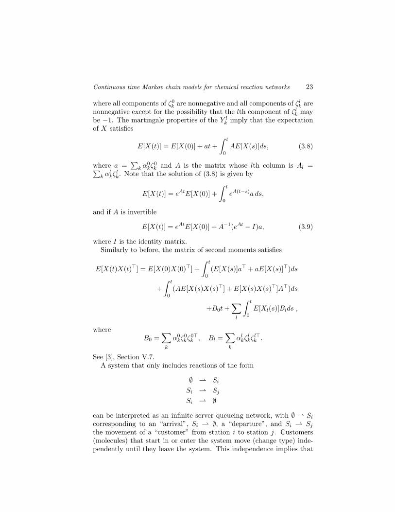
Continuous time Markov chain models for chemical reaction networks 23
where all components of ζ0k are nonnegative and all components of ζ lk are
nonnegative except for the possibility that the lth component of ζ lk maybe −1. The martingale properties of the Y l
k imply that the expectationof X satisfies
E[X(t)] = E[X(0)] + at+∫ t
0AE[X(s)]ds, (3.8)
where a =∑
k α0kζ
0k and A is the matrix whose lth column is Al =∑
k αlkζlk. Note that the solution of (3.8) is given by
E[X(t)] = eAtE[X(0)] +∫ t
0eA(t−s)a ds,
and if A is invertible
E[X(t)] = eAtE[X(0)] +A−1(eAt − I)a, (3.9)
where I is the identity matrix.Similarly to before, the matrix of second moments satisfies
E[X(t)X(t)>] = E[X(0)X(0)>] +∫ t
0(E[X(s)]a> + aE[X(s)]>)ds
+∫ t
0(AE[X(s)X(s)>] + E[X(s)X(s)>]A>)ds
+B0t+∑l
∫ t
0E[Xl(s)]Blds ,
whereB0 =
∑k
α0kζ
0kζ
0>k , Bl =
∑k
αlkζlkζl>k .
See [3], Section V.7.A system that only includes reactions of the form
∅ ⇀ Si
Si ⇀ Sj
Si ⇀ ∅
can be interpreted as an infinite server queueing network, with ∅ ⇀ Sicorresponding to an “arrival”, Si ⇀ ∅, a “departure”, and Si ⇀ Sjthe movement of a “customer” from station i to station j. Customers(molecules) that start in or enter the system move (change type) inde-pendently until they leave the system. This independence implies that

24
if {Xi(0)} are independent Poisson distributed random variables, then{Xi(t)} are independent Poisson distributed random variables for allt ≥ 0. Since the Poisson distribution is determined by its expectation,under the assumption of an independent Poisson initial distribution, thedistribution of X(t) is determined by E[X(t)], that is, by the solutionof (3.8).
Suppose that for each pair of species Si and Sj , it is possible for amolecule of Si to be converted, perhaps through a sequence of interme-diate steps, to a molecule of Sj . In addition, assume that the system isopen in the sense that there is at least one reaction of the form ∅⇀ Siand one reaction of the form Sj ⇀ ∅. Then A is invertible, so E[X(t)]is given by (3.9), and as t → ∞, eAt → 0 so E[X(t)] → −A−1a. Itfollows that the stationary distribution for X is given by a vector X ofindependent Poisson distributed random variables with E[X] = −A−1a.
If the system is closed so that the only reactions are of the formSi ⇀ Sj and the initial distribution is multinomial with parameters(n, p1(0), . . . , ps0(0)), that is, for k = (k1, . . . , ks0) with
∑i ki = n,
P{X(0) = k} =(
n
k1, . . . , ks0
)∏pi(0)ki ,
thenX(t) is multinomial (n, p1(t), . . . , ps0(t)), where p(t) = (p1(t), . . . , ps0(t))is given by
p(t) = eAtp(0).
Note that if the intensity for the reaction Si ⇀ Sj is κijXi(t), thenthe model is equivalent to n independent continuous-time Markov chainswith state space {1, . . . , s0} and transition intensities given by the κij .Consequently, if the independent chains have the same initial distribu-tion, p(0) = (p1(0), . . . , ps0(0)), then they have the same distributionat time t, namely p(t). The multinomial distribution with parameters(n, p) with p = limt→∞ p(t) will be a stationary distribution, but p isnot unique unless the assumption that every chemical species Si can beconverted into every other chemical species Sj holds.
See [18] for additional material on first order networks.
3.5 Product form stationary distributionsThe Poisson and multinomial stationary distributions discussed above
for unary systems are special cases of what are known as product formstationary distributions in the queueing literature. As noted in Chapter8 of [28] and discussed in detail in [2], a much larger class of reaction net-works also has product form stationary distributions. In fact, stochasticmodels of reaction networks that satisfy the conditions of the zero de-

Continuous time Markov chain models for chemical reaction networks 25
ficiency theorem of Feinberg [16] from deterministic reaction networktheory have this property.
Let S = {Si : i = 1, . . . , s0} denote the collection of chemical species,C = {νk, ν ′k : k = 1, . . . , r0} the collection of complexes, that is, thevectors that give either the inputs or the outputs of a reaction, andR = {νk → ν ′k : k = 1, . . . , r0} the collection of reactions. The triple,{S, C,R} determines the reaction network.
Definition 1.10 A chemical reaction network, {S, C,R}, is called weaklyreversible if for any reaction νk → ν ′k, there is a sequence of directed re-actions beginning with ν ′k as a source complex and ending with νk asa product complex. That is, there exist complexes ν1, . . . , νr such thatν ′k → ν1, ν1 → ν2, . . . , νr → νk ∈ R. A network is called reversible ifν ′k → νk ∈ R whenever νk → ν ′k ∈ R.
Let G be the directed graph with nodes given by the complexes C anddirected edges given by the reactions R = {νk → ν ′k}, and let G1, . . . ,G`denote the connected components of G. {Gj} are the linkage classes ofthe reaction network. Note that a reaction network is weakly reversibleif and only if the linkage classes are strongly connected.
Definition 1.11 S = span{νk→ν′k∈R}{ν′k − νk} is the stoichiometric
subspace of the network. For c ∈ Rs0, we say c + S and (c + S) ∩ Rs0>0
are the stoichiometric compatibility classes and positive stoichiometriccompatibility classes of the network, respectively. Denote dim(S) = s.
Definition 1.12 The deficiency of a chemical reaction network, {S, C,R},is δ = |C| − `− s, where |C| is the number of complexes, ` is the numberof linkage classes, and s is the dimension of the stoichiometric subspace.
For x, c ∈ Zs0≥0, we define cx ≡∏s0i=1 c
xii , where we interpret 00 = 1,
and x! ≡∏s0i=1 xi!. If for each complex η ∈ C, c ∈ Rs0
>0 satisfies∑k:νk=η
κkcνk =
∑k:ν′k=η
κkcνk , (3.10)
where the sum on the left is over reactions for which η is the sourcecomplex and the sum on the right is over those for which η is the productcomplex, then c is a special type of equilibrium of the system (you cansee this by summing each side of (3.10) over the complexes), and thenetwork is called complex balanced. The following is the Deficiency ZeroTheorem of Feinberg [16].
Theorem 1.13 Let {S, C,R} be a weakly reversible, deficiency zero chem-ical reaction network governed by deterministic mass action kinetics,
26
(3.2). Then, for any choice of rate constants κk, within each positivestoichiometric compatibility class there is precisely one equilibrium valuec, that is
∑k κkc
νk(ν ′k − νk) = 0, and that equilibrium value is locallyasymptotically stable relative to its compatibility class. Moreover, foreach η ∈ C, ∑
k:νk=η
κkcνk =
∑k:ν′k=η
κkcνk . (3.11)
For stochastically modeled systems we have the following theorem.
Theorem 1.14 Let {S, C,R} be a chemical reaction network with rateconstants κk. Suppose that the deterministically modeled system is com-plex balanced with equilibrium c ∈ Rm
>0. Then, for any irreducible com-municating equivalence class, Γ, the stochastic system has a product formstationary measure
π(x) = Mcx
x!, x ∈ Γ, (3.12)
where M is a normalizing constant.
Theorem 1.13 then shows that the conclusion of Theorem 1.14 holds,regardless of the choice of rate constants, for all stochastically modeledsystems with a reaction network that is weakly reversible and has adeficiency of zero.
3.6 Models with delayModeling chemical reaction networks as continuous-time Markov chains
is intuitively appealing and, as noted, consistent with the classical de-terministic law of mass action. Cellular reaction networks, however,include reactions for which the exponential timing of the simple Markovchain model is almost certainly wrong. These networks typically involveassembly processes (transcription or translation), referred to as elonga-tion, in which an enzyme or ribosome follows a DNA or RNA templateto create a new DNA, RNA, or protein molecule. The exponential hold-ing times in the Markov chain model reflect an assumption that once themolecules come together in the right configuration, the time it takes tocomplete the reaction is negligible. That is not, in general, the case forelongation. While each step of the assembly process might reasonablybe assumed to take an exponentially distributed time, the total time isa sum of such steps with the number of summands equal to the numberof nucleotides or amino acids. Since this number is large and essentially
Continuous time Markov chain models for chemical reaction networks 27
fixed, if the individual steps have small expectations, the total time thatthe reaction takes once the assembly is initiated may be closer to deter-ministic than exponential. See [5, 8] for examples of stochastic modelsof cellular reaction networks with delays.
One reasonable (though by no means only) way to incorporate delaysinto the models is to assume that for a reaction with deterministic delayξk that initiates at time t∗ the input molecules are lost at time t∗ and theproduct molecules are produced at time t∗+ξk. Noting that the numberof initiations of a reaction by time t can still be modeled by the countingprocess Yk(
∫ t0 λk(X(s))ds), we may let Γ1 denote those reactions with
no delay and Γ2 those with a delay, and conclude that the system shouldsatisfy the equation
X(t) = X(0) +∑k∈Γ1
Yk,1(∫ t
0λk(X(s))ds)(ν ′k − νk)
−∑k∈Γ2
Yk,2(∫ t
0λk(X(s))ds)νk +
∑k∈Γ2
Yk,2(∫ t−ξk
0λk(X(s))ds)ν ′k,
where we take X(s) ≡ 0, and hence λk(X(s)) ≡ 0, for s < 0. Existenceand uniqueness of solutions to this equation follow by the same jump byjump argument used in Section 2.2.
Simulation of reaction networks modeled with delay is no more dif-ficult than simulating those without delay. For example, the aboveequation suggests a simulation strategy equivalent to the next reactionmethod [1, 19]. There are also analogues of the stochastic simulationalgorithm, or Gillespie’s algorithm [8].
4. Multiple scalesThe classical scaling that leads to the deterministic law of mass ac-
tion assumes that all chemical species are present in numbers of thesame order of magnitude. For reaction networks in biological cells, thisassumption is usually clearly violated. Consequently, models derived bythe classical scaling may not be appropriate. For these networks somespecies are present in such small numbers that they should be modeledby discrete variables while others are present in large enough numbersto reasonably be modeled by continuous variables. These large numbersmay still differ by several orders of magnitude, so normalizing all “large”quantities in the same way may still be inappropriate. Consequently,methods are developed in [4], [26], and [27] for deriving simplified mod-els in which different species numbers are normalized in different waysappropriate to their numbers in the system.

28
4.1 Derivation of the Michaelis-Menten equationPerhaps the best known examples of reaction networks in which mul-
tiple scales play a role are models that lead to the Michaelis-Mentenequation. Darden [9, 10] gave a derivation starting from a stochasticmodel, and we prove his result using our methodology.
Consider the reaction system
S1 + S2
κ′1κ′2
S3κ′3⇀S4 + S2,
where S1 is the substrate, S2 the enzyme, S3 the enzyme-substrate com-plex, and S4 the product. Assume that the parameters scale so that
ZN1 (t) = ZN1 (0)−N−1Y1(N∫ t
0κ1Z
N1 (s)ZN2 (s)ds)
+N−1Y2(N∫ t
0κ2Z
N3 (s)ds)
ZN2 (t) = ZN2 (0)− Y1(N∫ t
0κ1Z
N1 (s)ZN2 (s)ds) + Y2(N
∫ t
0κ2Z
N3 (s)ds)
+Y3(N∫ t
0κ3Z
N3 (s)ds)
ZN3 (t) = ZN2 (0) + Y1(N∫ t
0κ1Z
N1 (s)ZN2 (s)ds)− Y2(N
∫ t
0κ2Z
N3 (s)ds)
−Y3(N∫ t
0κ3Z
N3 (s)ds)
ZN4 (t) = N−1Y3(N∫ t
0κ3Z
N3 (s)ds),
where κ1, κ2, κ3 do not depend upon N . Note that we scale the numbersof molecules of the substrate and the product as in the previous section,but we leave the enzyme and enzyme-substrate variables discrete. Notealso that M = ZN3 (t) + ZN2 (t) is constant, and define
ZN2 (t) =∫ t
0ZN2 (s)ds = Mt−
∫ t
0ZN3 (s)ds.
Theorem 1.15 Assume that ZN1 (0) → Z1(0) and that M does not de-pend on N . Then (ZN1 , Z
N2 ) converges to (Z1(t), Z2(t)) satisfying
Continuous time Markov chain models for chemical reaction networks 29
Z1(t) = Z1(0)−∫ t
0κ1Z1(s) ˙
Z2(s)ds+∫ t
0κ2(M − ˙
Z2(s))ds (4.1)
0 = −∫ t
0κ1Z1(s) ˙
Z2(s)ds+∫ t
0(κ2 + κ3)(M − ˙
Z2(s))ds,
and hence ˙Z2(s) = (κ2+κ3)M
κ2+κ3+κ1Z1(s) and
Z1(t) = − Mκ1κ3Z1(t)κ2 + κ3 + κ1Z1(s)
. (4.2)
Proof. Relative compactness of the sequence (ZN1 , ZN2 ) is straightfor-
ward, that is, at least along a subsequence, we can assume that (ZN1 , ZN2 )
converges in distribution to a continuous process (Z1, Z2) (which turnsout to be deterministic). Dividing the second equation by N and passingto the limit, we see (Z1, Z2) must satisfy
0 = −∫ t
0κ1Z1(s)dZ2(s) + (κ2 + κ3)Mt−
∫ t
0(κ2 + κ3)dZ2(s). (4.3)
Since Z2 is Lipschitz, it is absolutely continuous, and rewriting (4.3)in terms of the derivative gives the second equation in (4.1). The firstequation follows by a similar argument. �
Of course, (4.2) is the Michaelis-Menten equation.
4.2 Scaling species numbers and rate constantsAssume that we are given a model of the form
X(t) = X(0) +∑k
Yk(∫ t
0λ′k(X(s))ds)(ν ′k − νk)
where the λ′k are of the form
λ′k(x) = κ′k∏i
νik!∏i
(xiνik
).
Let N0 � 1. For each species i, define the normalized abundance (orsimply, the abundance) by
Zi(t) = N−αi0 Xi(t),
30
where αi ≥ 0 should be selected so that Zi = O(1). The abundancemay be the species number (αi = 0) or the species concentration orsomething else.
Since the rate constants may also vary over several orders of magni-tude, we write κ′k = κkN
βk0 where the βk are selected so that κk = O(1).
For a binary reaction
κ′kxixj = Nβk+αi+αj0 κkzizj ,
and we can writeβk + αi + αj = βk + νk · α.
We also have,
κ′kxi = Nβk+νk·α0 zi, κ′kxi(xi − 1) = Nβk+νk·α
0 zi(zi −N−αi0 ),
with similar expressions for intensities involving higher order reactions.We replace N0 by N in the above expressions and consider a family
of models,
ZNi (t) = ZNi (0) +∑k
N−αiYk(∫ t
0Nβk+νk·αλk(ZN (s))ds)(ν ′ik − νik),
where the original model is Z = ZN0 . Note that for reactions of theform 2Si ⇀ *, where ∗ represents an arbitrary linear combination of thespecies, the rate is Nβk+2αiZNi (t)(ZNi (t)−N−αi), so if αi > 0, we shouldwrite λNk instead of λk, but to simplify notation, we will simply writeλk.
We have a family of models indexed by N for which N = N0 givesthe “correct” or original model. Other values of N and any limits asN →∞ (perhaps with a change of time-scale) give approximate models.The challenge is to select the αi and the βk in a reasonable way, butonce that is done, the initial condition for index N is given by
ZNi (0) = N−αi⌊Nαi
Xi(0)Nαi
0
⌋,
where bzc is the integer part of z and the Xi(0) are the initial speciesnumbers in the original model.
Allowing a change of time-scale, where t is replaced by tNγ , supposelimN→∞ Z
Ni (·Nγ) = Z∞i . Then we should have
Xi(t) ≈ Nαi0 Z∞i (tN−γ0 ).
Continuous time Markov chain models for chemical reaction networks 31
4.3 Determining the scaling exponentsThere are, of course, many ways of selecting the αi and βk, but we
want to make this selection so that there are limiting models that givereasonable approximations for the original model. Consequently, we lookfor natural constraints on the αi and βk.
For example, suppose that the rate constants satisfy
κ′1 ≥ κ′2 ≥ · · · ≥ κ′r0 .
Then it seems natural to select
β1 ≥ · · · ≥ βr0 ,
although it may be reasonable to impose this constraint separately forthe binary reactions and the unary reactions.
To get a sense of the issues involved in selecting exponents that leadto reasonable limits, consider a reaction network in which the reactionsinvolving S3 are
S1 + S2 ⇀ S3 + S4 S3 + S5 ⇀ S6.
Then
ZN3 (t) = ZN3 (0) +N−α3Y1(Nβ1+α1+α2
∫ t
0κ1Z
N1 (s)ZN2 (s)ds)
−N−α3Y2(Nβ2+α3+α5
∫ t
0κ2Z
N3 (s)ZN5 (s)ds) ,
or scaling time
ZN3 (tNγ) = ZN3 (0) +N−α3Y1(Nβ1+α1+α2+γ
∫ t
0κ1Z
N1 (sNγ)ZN2 (sNγ)ds)
−N−α3Y2(Nβ2+α3+α5+γ
∫ t
0κ2Z
N3 (sNγ)ZN5 (sNγ)ds) .
Assuming that for the other species in the system ZNi = O(1), we seethat ZN3 = O(1) if
(β1 + α1 + α2 + γ) ∨ (β2 + α3 + α5 + γ) ≤ α3
or ifβ1 + α1 + α2 = β2 + α3 + α5 > α3.
Note that in the latter case, we would expect ZN3 (t) ≈ κ1ZN1 (t)ZN2 (t)
κ2ZN5 (t). If
these conditions both fail, then either ZN3 will blow up as N → ∞ orwill be driven to zero.
32
With this example in mind, define ZN,γi (t) = ZNi (tNγ) so
ZN,γi (t) = ZNi (0)+∑k
N−αiYk(∫ t
0Nγ+βk+νk·αλk(ZN,γ(s))ds)(ν ′ik−νik).
Recalling that ζk = ν ′k − νk, for θi ≥ 0, consider∑i
θiNαiZN,γi (t)
=∑i
θiNαiZNi (0) +
∑k
Yk(∫ t
0Nγ+βk+νk·αλk(ZN,γ(s))ds)〈θ, ζk〉,
where 〈θ, ζk〉 =∑
i θiζik, and define αθ = max{αi : θi > 0}. If allZN,γi = O(1), then the left side is O(Nαθ), and as in the single speciesexample above, we must have
γ + max{βk + νk · α : 〈θ, ζk〉 6= 0} ≤ αθ. (4.4)
or
max{βk + νk · α : 〈θ, ζk〉 > 0} = max{βk + νk · α : 〈θ, ζk〉 < 0}. (4.5)
Note that (4.4) is really a constraint on the time-scale determined by γsaying that if (4.5) fails for some θ, then γ must satisfy
γ ≤ αθ −max{βk + νk · α : 〈θ, ζk〉 6= 0}.
The value of γ given by
γi = αi −max{βk + νk · α : ζik 6= 0}
gives the natural time-scale for Si in the sense that ZN,γ
i is neither asymp-totically constant nor too rapidly oscillating to have a limit. The γi arevalues of γ for which interesting limits may hold. Linear combinations〈θ, ZN,γ〉 may have time-scales
γθ = αθ −max{βk + νk · α : 〈θ, ζk〉 6= 0}
that are different from all of the species time-scales and may give aux-iliary variables (see, for example, [14]) whose limits capture interestingproperties of the system.
The equation (4.5) is called the balance equation, and together, thealternative (4.5) and (4.4) is referred to as the balance condition. Toemploy this approach to the identification of simplified models, it is
Continuous time Markov chain models for chemical reaction networks 33
not necessary to solve the balance equations for every choice of θ. Theequations that fail simply place restrictions on the time-scales γ that canbe used without something blowing up. The goal is to find αi and βkthat give useful limiting models, and solving some subset of the balanceequations can be a useful first step. Natural choices of θ in selecting thesubset of balance equations to solve include those for which 〈θ, ζk〉 = 0for one or more of the ζk. See Section 3.4 of [26] for a more detaileddiscussion.
In the next subsection, we apply the balance conditions to identifyexponents useful in deriving a reduced model for a simple reaction net-work. For an application to a much more complex model of the heatshock response in E. coli, see [25].
4.4 An application of the balance conditionsConsider the simple example
∅κ′1⇀S1
κ′2κ′3
S2, S1 + S2κ′4⇀S3
Assume κ′k = κkNβk0 . Then a useful subset of the balance equations is
S2 β2 + α1 = (β3 + α2) ∨ (β4 + α1 + α2)S1 β1 ∨ (β3 + α2) = (β2 + α1) ∨ (β4 + α1 + α2)S3 β4 + α1 + α2 = −∞S1 + S2 β1 = β4 + α1 + α2
where we take the maximum of the empty set to be −∞. Of course, itis not possible to select parameters satisfying the balance equation forS3, so we must restrict γ by
γ ≤ α3 − (β4 + α1 + α2). (4.6)
Let α1 = 0 and β1 = β2 > β3 = β4, so balance for S1, S2, and S1 +S2
is satisfied if α2 = β2 − β3, which we assume. Taking α3 = α2, (4.6)becomes
γ ≤ −β4 = −β3.
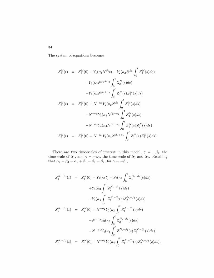
34
The system of equations becomes
ZN1 (t) = ZN1 (0) + Y1(κ1Nβ1t)− Y2(κ2N
β2
∫ t
0ZN1 (s)ds)
+Y3(κ3Nβ3+α2
∫ t
0ZN2 (s)ds)
−Y4(κ4Nβ4+α2
∫ t
0ZN1 (s)ZN2 (s)ds)
ZN2 (t) = ZN2 (0) +N−α2Y2(κ2Nβ2
∫ t
0ZN1 (s)ds)
−N−α2Y3(κ3Nβ3+α2
∫ t
0ZN2 (s)ds)
−N−α2Y4(κ4Nβ4+α2
∫ t
0ZN1 (s)ZN2 (s)ds)
ZN3 (t) = ZN3 (0) +N−α3Y4(κ4Nβ4+α2
∫ t
0ZN1 (s)ZN2 (s)ds).
There are two time-scales of interest in this model, γ = −β1, thetime-scale of S1, and γ = −β3, the time-scale of S2 and S3. Recallingthat α2 + β3 = α2 + β4 = β1 = β2, for γ = −β1,
ZN,−β11 (t) = ZN1 (0) + Y1(κ1t)− Y2(κ2
∫ t
0ZN,−β1
1 (s)ds)
+Y3(κ3
∫ t
0ZN,−β1
2 (s)ds)
−Y4(κ4
∫ t
0ZN,−β1
1 (s)ZN,−β12 (s)ds)
ZN,−β12 (t) = ZN2 (0) +N−α2Y2(κ2
∫ t
0ZN,−β1
1 (s)ds)
−N−α2Y3(κ3
∫ t
0ZN,−β1
2 (s)ds)
−N−α2Y4(κ4
∫ t
0ZN,−β1
1 (s)ZN,−β12 (s)ds)
ZN,−β13 (t) = ZN3 (0) +N−α3Y4(κ4
∫ t
0ZN,−β1
1 (s)ZN,−β12 (s)ds),
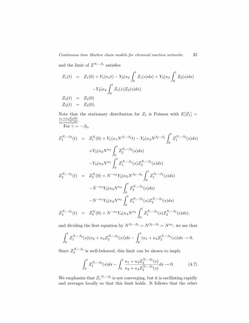
Continuous time Markov chain models for chemical reaction networks 35
and the limit of ZN,−β1 satisfies
Z1(t) = Z1(0) + Y1(κ1t)− Y2(κ2
∫ t
0Z1(s)ds) + Y3(κ3
∫ t
0Z2(s)ds)
−Y4(κ4
∫ t
0Z1(s)Z2(s)ds)
Z2(t) = Z2(0)Z3(t) = Z3(0).
Note that the stationary distribution for Z1 is Poisson with E[Z1] =κ1+κ3Z2(0)κ2+κ4Z2(0) .
For γ = −β3,
ZN,−β31 (t) = ZN1 (0) + Y1(κ1N
β1−β3t)− Y2(κ2Nβ2−β3
∫ t
0ZN,−β3
1 (s)ds)
+Y3(κ3Nα2
∫ t
0ZN,−β3
2 (s)ds)
−Y4(κ4Nα2
∫ t
0ZN,−β3
1 (s)ZN,−β32 (s)ds)
ZN,−β32 (t) = ZN2 (0) +N−α2Y2(κ2N
β2−β3
∫ t
0ZN,−β3
1 (s)ds)
−N−α2Y3(κ3Nα2
∫ t
0ZN,−β3
2 (s)ds)
−N−α2Y4(κ4Nα2
∫ t
0ZN,−β3
1 (s)ZN,−β32 (s)ds)
ZN,−β33 (t) = ZN3 (0) +N−α3Y4(κ4N
α2
∫ t
0ZN,−β3
1 (s)ZN,−β32 (s)ds),
and dividing the first equation by Nβ1−β3 = Nβ2−β3 = Nα2 , we see that∫ t
0ZN,−β3
1 (s)(κ2 + κ4ZN,−β32 (s))ds−
∫ t
0(κ1 + κ3Z
N,−β32 (s))ds→ 0.
Since ZN,−β32 is well-behaved, this limit can be shown to imply∫ t
0ZN,−β3
1 (s)ds−∫ t
0
κ1 + κ3ZN,−β32 (s)
κ2 + κ4ZN,−β32 (s)
ds→ 0. (4.7)
We emphasize that Z1N,−β3 is not converging, but it is oscillating rapidly
and averages locally so that this limit holds. It follows that the other
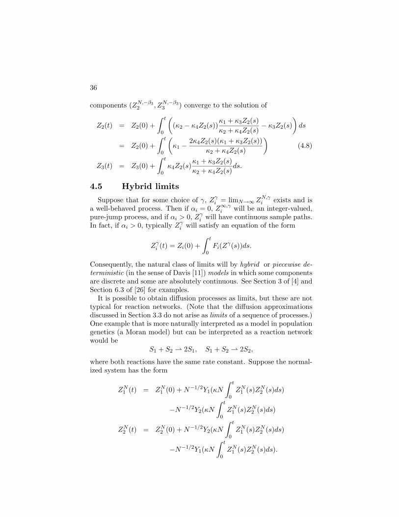
36
components (ZN,−β32 , ZN,−β3
3 ) converge to the solution of
Z2(t) = Z2(0) +∫ t
0
((κ2 − κ4Z2(s))
κ1 + κ3Z2(s)κ2 + κ4Z2(s)
− κ3Z2(s))ds
= Z2(0) +∫ t
0
(κ1 −
2κ4Z2(s)(κ1 + κ3Z2(s))κ2 + κ4Z2(s)
)(4.8)
Z3(t) = Z3(0) +∫ t
0κ4Z2(s)
κ1 + κ3Z2(s)κ2 + κ4Z2(s)
ds.
4.5 Hybrid limits
Suppose that for some choice of γ, Zγi = limN→∞ ZN,γi exists and is
a well-behaved process. Then if αi = 0, Z∞,γi will be an integer-valued,pure-jump process, and if αi > 0, Zγi will have continuous sample paths.In fact, if αi > 0, typically Zγi will satisfy an equation of the form
Zγi (t) = Zi(0) +∫ t
0Fi(Zγ(s))ds.
Consequently, the natural class of limits will by hybrid or piecewise de-terministic (in the sense of Davis [11]) models in which some componentsare discrete and some are absolutely continuous. See Section 3 of [4] andSection 6.3 of [26] for examples.
It is possible to obtain diffusion processes as limits, but these are nottypical for reaction networks. (Note that the diffusion approximationsdiscussed in Section 3.3 do not arise as limits of a sequence of processes.)One example that is more naturally interpreted as a model in populationgenetics (a Moran model) but can be interpreted as a reaction networkwould be
S1 + S2 ⇀ 2S1, S1 + S2 ⇀ 2S2,
where both reactions have the same rate constant. Suppose the normal-ized system has the form
ZN1 (t) = ZN1 (0) +N−1/2Y1(κN∫ t
0ZN1 (s)ZN2 (s)ds)
−N−1/2Y2(κN∫ t
0ZN1 (s)ZN2 (s)ds)
ZN2 (t) = ZN2 (0) +N−1/2Y2(κN∫ t
0ZN1 (s)ZN2 (s)ds)
−N−1/2Y1(κN∫ t
0ZN1 (s)ZN2 (s)ds).
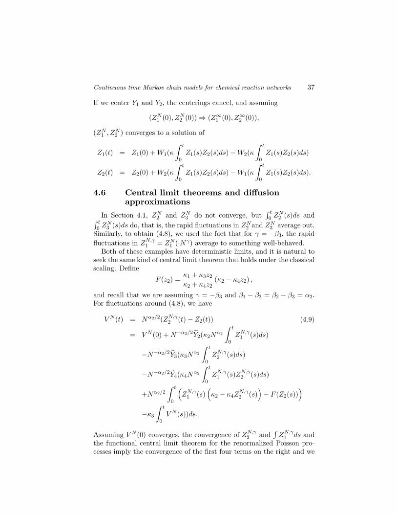
Continuous time Markov chain models for chemical reaction networks 37
If we center Y1 and Y2, the centerings cancel, and assuming
(ZN1 (0), ZN2 (0))⇒ (Z∞1 (0), Z∞2 (0)),
(ZN1 , ZN2 ) converges to a solution of
Z1(t) = Z1(0) +W1(κ∫ t
0Z1(s)Z2(s)ds)−W2(κ
∫ t
0Z1(s)Z2(s)ds)
Z2(t) = Z2(0) +W2(κ∫ t
0Z1(s)Z2(s)ds)−W1(κ
∫ t
0Z1(s)Z2(s)ds).
4.6 Central limit theorems and diffusionapproximations
In Section 4.1, ZN2 and ZN3 do not converge, but∫ t
0 ZN2 (s)ds and∫ t
0 ZN3 (s)ds do, that is, the rapid fluctuations in ZN2 and ZN3 average out.
Similarly, to obtain (4.8), we used the fact that for γ = −β3, the rapidfluctuations in ZN,γ1 = ZN1 (·Nγ) average to something well-behaved.
Both of these examples have deterministic limits, and it is natural toseek the same kind of central limit theorem that holds under the classicalscaling. Define
F (z2) =κ1 + κ3z2
κ2 + κ4z2(κ2 − κ4z2) ,
and recall that we are assuming γ = −β3 and β1 − β3 = β2 − β3 = α2.For fluctuations around (4.8), we have
V N (t) = Nα2/2(ZN,γ2 (t)− Z2(t)) (4.9)
= V N (0) +N−α2/2Y2(κ2Nα2
∫ t
0ZN,γ1 (s)ds)
−N−α2/2Y3(κ3Nα2
∫ t
0ZN,γ2 (s)ds)
−N−α2/2Y4(κ4Nα2
∫ t
0ZN,γ1 (s)ZN,γ2 (s)ds)
+Nα2/2
∫ t
0
(ZN,γ1 (s)
(κ2 − κ4Z
N,γ2 (s)
)− F (Z2(s))
)−κ3
∫ t
0V N (s))ds.
Assuming V N (0) converges, the convergence of ZN,γ2 and∫ZN,γ1 ds and
the functional central limit theorem for the renormalized Poisson pro-cesses imply the convergence of the first four terms on the right and we
38
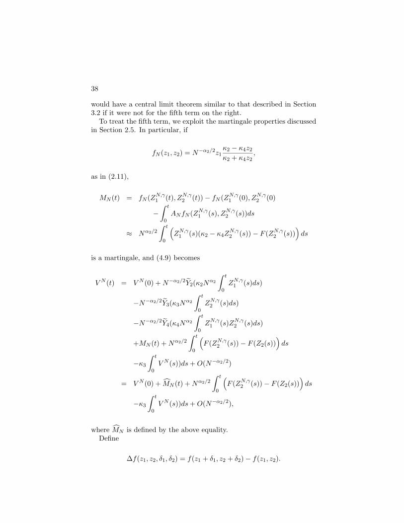
would have a central limit theorem similar to that described in Section3.2 if it were not for the fifth term on the right.
To treat the fifth term, we exploit the martingale properties discussedin Section 2.5. In particular, if
fN (z1, z2) = N−α2/2z1κ2 − κ4z2
κ2 + κ4z2,
as in (2.11),
MN (t) = fN (ZN,γ1 (t), ZN,γ2 (t))− fN (ZN,γ1 (0), ZN,γ2 (0)
−∫ t
0ANfN (ZN,γ1 (s), ZN,γ2 (s))ds
≈ Nα2/2
∫ t
0
(ZN,γ1 (s)(κ2 − κ4Z
N,γ2 (s))− F (ZN,γ2 (s))
)ds
is a martingale, and (4.9) becomes
V N (t) = V N (0) +N−α2/2Y2(κ2Nα2
∫ t
0ZN,γ1 (s)ds)
−N−α2/2Y3(κ3Nα2
∫ t
0ZN,γ2 (s)ds)
−N−α2/2Y4(κ4Nα2
∫ t
0ZN,γ1 (s)ZN,γ2 (s)ds)
+MN (t) +Nα2/2
∫ t
0
(F (ZN,γ2 (s))− F (Z2(s))
)ds
−κ3
∫ t
0V N (s))ds+O(N−α2/2)
= V N (0) + MN (t) +Nα2/2
∫ t
0
(F (ZN,γ2 (s))− F (Z2(s))
)ds
−κ3
∫ t
0V N (s))ds+O(N−α2/2),
where MN is defined by the above equality.Define
∆f(z1, z2, δ1, δ2) = f(z1 + δ1, z2 + δ2)− f(z1, z2).
Continuous time Markov chain models for chemical reaction networks 39
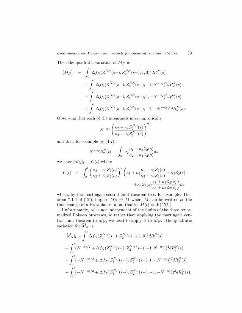
Then the quadratic variation of MN is
[MN ]t =∫ t
0∆fN (ZN,γ1 (s−), ZN,γ2 (s−), 1, 0)2dRN1 (s)
+∫ t
0∆fN (ZN,γ1 (s−), ZN,γ2 (s−),−1, N−α2)2dRN2 (s)
+∫ t
0∆fN (ZN,γ1 (s−), ZN,γ2 (s−), 1,−N−α2)2dRN3 (s)
+∫ t
0∆fN (ZN,γ1 (s−), ZN,γ2 (s−),−1,−N−α2)2dRN4 (s).
Observing that each of the integrands is asymptotically
N−α2
(κ2 − κ4Z
N,γ2 (s)
κ2 + κ4ZN,γ2 (s)
)2
and that, for example by (4.7),
N−α2RN2 (t)→∫ t
0κ2κ1 + κ3Z2(s)κ2 + κ4Z2(s)
ds,
we have [MN ]t → C(t) where
C(t) =∫ t
0
(κ2 − κ4Z2(s)κ2 + κ4Z2(s)
)2(κ1 + κ2
κ1 + κ3Z2(s)κ2 + κ4Z2(s)
+ κ3Z2(s)
+κ4Z2(s)κ1 + κ3Z2(s)κ2 + κ4Z2(s)
)ds,
which, by the martingale central limit theorem (see, for example, The-orem 7.1.4 of [15]), implies MN ⇒ M where M can be written as thetime change of a Brownian motion, that is, M(t) = W (C(t)).
Unfortunately, M is not independent of the limits of the three renor-malized Poisson processes, so rather than applying the martingale cen-tral limit theorem to MN , we need to apply it to MN . The quadraticvariation for MN is
[MN ]t =∫ t
0∆fN (ZN,γ1 (s−), ZN,γ2 (s−), 1, 0)2dRN1 (s)
+∫ t
0(N−α2/2 + ∆fN (ZN,γ1 (s−), ZN,γ2 (s−),−1, N−α2))2dRN2 (s)
+∫ t
0(−N−α2/2 + ∆fN (ZN,γ1 (s−), ZN,γ2 (s−), 1,−N−α2))2dRN3 (s)
+∫ t
0(−N−α2/2 + ∆fN (ZN,γ1 (s−), ZN,γ2 (s−),−1,−N−α2))2dRN4 (s),
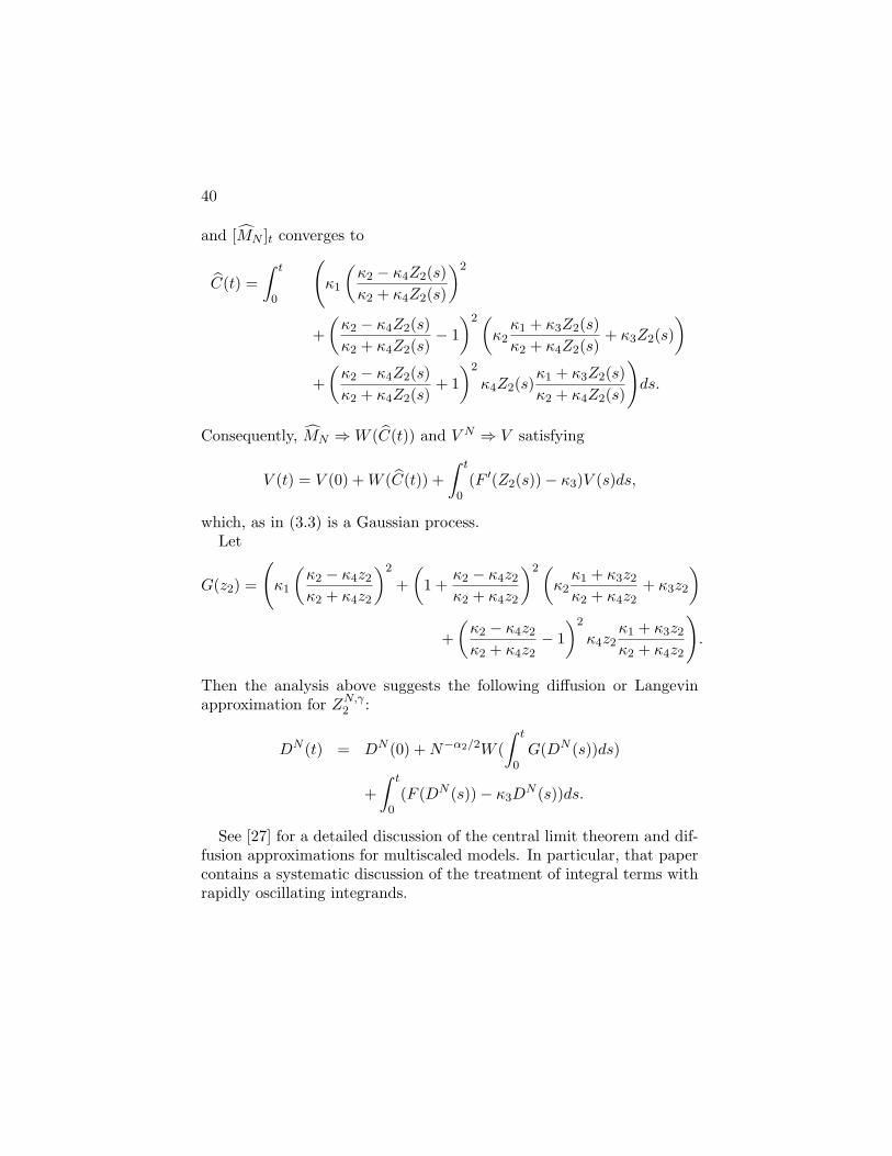
40
and [MN ]t converges to
C(t) =∫ t
0
(κ1
(κ2 − κ4Z2(s)κ2 + κ4Z2(s)
)2
+(κ2 − κ4Z2(s)κ2 + κ4Z2(s)
− 1)2(
κ2κ1 + κ3Z2(s)κ2 + κ4Z2(s)
+ κ3Z2(s))
+(κ2 − κ4Z2(s)κ2 + κ4Z2(s)
+ 1)2
κ4Z2(s)κ1 + κ3Z2(s)κ2 + κ4Z2(s)
)ds.
Consequently, MN ⇒W (C(t)) and V N ⇒ V satisfying
V (t) = V (0) +W (C(t)) +∫ t
0(F ′(Z2(s))− κ3)V (s)ds,
which, as in (3.3) is a Gaussian process.Let
G(z2) =
(κ1
(κ2 − κ4z2
κ2 + κ4z2
)2
+(
1 +κ2 − κ4z2
κ2 + κ4z2
)2(κ2κ1 + κ3z2
κ2 + κ4z2+ κ3z2
)
+(κ2 − κ4z2
κ2 + κ4z2− 1)2
κ4z2κ1 + κ3z2
κ2 + κ4z2
).
Then the analysis above suggests the following diffusion or Langevinapproximation for ZN,γ2 :
DN (t) = DN (0) +N−α2/2W (∫ t
0G(DN (s))ds)
+∫ t
0(F (DN (s))− κ3D
N (s))ds.
See [27] for a detailed discussion of the central limit theorem and dif-fusion approximations for multiscaled models. In particular, that papercontains a systematic discussion of the treatment of integral terms withrapidly oscillating integrands.
Bibliography
[1] Anderson, David F. (2007). A modified next reaction method forsimulating chemical systems with time dependent propensities anddelays. J. Chem. Phys., 127(21):214107.
[2] Anderson, David F., Craciun, Gheorge, and Kurtz, Thomas G.(2010). Product-form stationary distributions for deficiency zerochemical reaction networks. Bull. Math. Biol.
[3] Athreya, Krishna B. and Ney, Peter E. (1972). Branching processes.Springer-Verlag, New York. Die Grundlehren der mathematischenWissenschaften, Band 196.
[4] Ball, Karen, Kurtz, Thomas G., Popovic, Lea, and Rempala, Greg(2006). Asymptotic analysis of multiscale approximations to reactionnetworks. Ann. Appl. Probab., 16(4):1925–1961.
[5] Barrio, Manuel, Burrage, Kevin, Leier, Andre, and Tian, Tianhai(2006). Oscillatory regulation of Hes1: Discrete stochastic delay mod-elling and simulation. PLoS Comp. Biol., 2:1017–1030.
[6] Bartholomay, Anthony F. (1958). Stochastic models for chemicalreactions. I. Theory of the unimolecular reaction process. Bull. Math.Biophys., 20:175–190.
[7] Bartholomay, Anthony F. (1959). Stochastic models for chemicalreactions. II. The unimolecular rate constant. Bull. Math. Biophys.,21:363–373.
[8] Bratsun, Dmitri, Volfson, Dmitri, Tsimring, Lev S., and Hasty,Jeff (2005). Delay-induced stochastic oscillations in gene regulation.PNAS, 102:14593 – 14598.
[9] Darden, Thomas (1979). A pseudo-steady state approximation forstochastic chemical kinetics. Rocky Mountain J. Math., 9(1):51–71.
42
Conference on Deterministic Differential Equations and StochasticProcesses Models for Biological Systems (San Cristobal, N.M., 1977).
[10] Darden, Thomas A. (1982). Enzyme kinetics: stochastic vs. de-terministic models. In Instabilities, bifurcations, and fluctuations inchemical systems (Austin, Tex., 1980), pages 248–272. Univ. TexasPress, Austin, TX.
[11] Davis, M. H. A. (1993). Markov models and optimization, volume 49of Monographs on Statistics and Applied Probability. Chapman & Hall,London.
[12] Delbruck, Max (1940). Statistical fluctuations in autocatalytic re-actions. The Journal of Chemical Physics, 8(1):120–124.
[13] Donsker, Monroe D. (1951). An invariance principle for certainprobability limit theorems. Mem. Amer. Math. Soc.,, 1951(6):12.
[14] E, Weinan, Liu, Di, and Vanden-Eijnden, Eric (2005). Nestedstochastic simulation algorithm for chemical kinetic systems with dis-parate rates. The Journal of Chemical Physics, 123(19):194107.
[15] Ethier, Stewart N. and Kurtz, Thomas G. (1986). Markov processes.Wiley Series in Probability and Mathematical Statistics: Probabil-ity and Mathematical Statistics. John Wiley & Sons Inc., New York.Characterization and convergence.
[16] Feinberg, Martin (1987). Chemical reaction network structure andthe stability of complex isothermal reactors i. the deficiency zero anddeficiency one theorems. Chem. Engr. Sci., 42(10):2229–2268.
[17] Feinberg, Martin (1988). Chemical reaction network structure andthe stability of complex isothermal reactors ii. multiple steady statesfor networks of deficiency one. Chem. Engr. Sci., 43(1):1–25.
[18] Gadgil, Chetan, Lee, Chang Hyeong, and Othmer, Hans G. (2005).A stochastic analysis of first-order reaction networks. Bull. Math.Biol., 67(5):901–946.
[19] Gibson, M. A. and J., Bruck (2000). Efficient exact simulation ofchemical systems with many species and many channels. J. Phys.Chem. A, 104(9):1876–1889.
[20] Gillespie, Daniel T. (1976). A general method for numerically sim-ulating the stochastic time evolution of coupled chemical reactions. J.Computational Phys., 22(4):403–434.
BIBLIOGRAPHY 43
[21] Gillespie, Daniel T. (1977). Exact stochastic simulation of coupledchemical reactions. J. Phys. Chem., 81:2340–61.
[22] Gillespie, Daniel T. (1992). A rigorous derivation of the chemicalmaster equation. Physica A, 188:404–425.
[23] Gillespie, Daniel T. (2001). Approximate accelerated stochasticsimulation of chemically reacting systems. The Journal of ChemicalPhysics, 115(4):1716–1733.
[24] Jacod, Jean (1974/75). Multivariate point processes: predictableprojection, Radon-Nikodym derivatives, representation of martin-gales. Z. Wahrscheinlichkeitstheorie und Verw. Gebiete, 31:235–253.
[25] Kang, Hye-Won (2009). The multiple scaling approximation in theheat shock model of e. coli. In Preparation.
[26] Kang, Hye-Won and Kurtz, Thomas G. (2010). Separation of time-scales and model reduction for stochastic reaction networks. In prepa-ration.
[27] Kang, Hye-Won, Kurtz, Thomas G., and Popovic, Lea (2010). Dif-fusion approximations for multiscale chemical reaction models. inpreparation.
[28] Kelly, Frank P. (1979). Reversibility and stochastic networks. JohnWiley & Sons Ltd., Chichester. Wiley Series in Probability and Math-ematical Statistics.
[29] Kolmogorov, A. N. (1956). Foundations of the theory of probability.Chelsea Publishing Co., New York. Translation edited by NathanMorrison, with an added bibliography by A. T. Bharucha-Reid.
[30] Komlos, J., Major, P., and Tusnady, G. (1975). An approxima-tion of partial sums of independent RV’s and the sample DF. I. Z.Wahrscheinlichkeitstheorie und Verw. Gebiete, 32:111–131.
[31] Komlos, J., Major, P., and Tusnady, G. (1976). An approxima-tion of partial sums of independent RV’s, and the sample DF. II. Z.Wahrscheinlichkeitstheorie und Verw. Gebiete, 34(1):33–58.
[32] Kurtz, Thomas G. (1970). Solutions of ordinary differential equa-tions as limits of pure jump Markov processes. J. Appl. Probability,7:49–58.
[33] Kurtz, Thomas G. (1971). Limit theorems for sequences of jumpMarkov processes approximating ordinary differential processes. J.Appl. Probability, 8:344–356.
44
[34] Kurtz, Thomas G. (1972). The relationship between stochasticand deterministic models for chemical reactions. J. Chem. Phys.,57(7):2976–2978.
[35] Kurtz, Thomas G. (1977/78). Strong approximation theoremsfor density dependent Markov chains. Stochastic Processes Appl.,6(3):223–240.
[36] Kurtz, Thomas G. (1980). Representations of Markov processes asmultiparameter time changes. Ann. Probab., 8(4):682–715.
[37] Kurtz, Thomas G. (2007). The Yamada-Watanabe-Engelbert the-orem for general stochastic equations and inequalities. Electron. J.Probab., 12:951–965.
[38] Kurtz, Thomas G. (2010). Equivalence of stochastic equations andmartingale problems. In Stochastic Analysis 2010. Springer.
[39] McQuarrie, Donald A. (1967). Stochastic approach to chemicalkinetics. J. Appl. Probability, 4:413–478.
[40] Meyer, P. A. (1971). Demonstration simplifiee d’un theoreme deKnight. In Seminaire de Probabilites, V (Univ. Strasbourg, anneeuniversitaire 1969–1970), pages 191–195. Lecture Notes in Math., Vol.191. Springer, Berlin.
[41] Ross, Sheldon (1984). A first course in probability. Macmillan Co.,New York, second edition.
[42] van Kampen, N. G. (1961). A power series expansion of the masterequation. Canad. J. Phys., 39:551–567.