continuous tensor network states - lmu
TRANSCRIPT
Continuous Tensor Network States
Teresa Dimitra Karanikolaou
Munich 2020


Continuous Tensor Network States
Teresa Dimitra Karanikolaou
Master’s Thesis
Ludwig–Maximilians–Universitat and Technische Universitat
Munchen
Munich, 23/01/2020
Supervisor: Prof. Dr. I. Cirac
Advisor: Dr. A. Tilloy

iv

Contents
Abstract ix
Introduction 1
1 Theoretical Background 51.1 Tensor Network States . . . . . . . . . . . . . . . . . . . . . . . . . . . . . 5
1.1.1 Matrix Product States (MPS) . . . . . . . . . . . . . . . . . . . . . 61.1.2 Area Law . . . . . . . . . . . . . . . . . . . . . . . . . . . . . . . . 91.1.3 Projected Entangled Pairs State (PEPS) . . . . . . . . . . . . . . . 11
1.2 Continuous Matrix Product States (cMPS) . . . . . . . . . . . . . . . . . . 121.2.1 Correlation functions and expectation values . . . . . . . . . . . . . 131.2.2 Link with discrete MPS . . . . . . . . . . . . . . . . . . . . . . . . 141.2.3 Application on the Lieb-Liniger Model . . . . . . . . . . . . . . . . 15
1.3 Continuous Tensor Networks States (cTNS) . . . . . . . . . . . . . . . . . 161.3.1 Correlation functions and expectation values . . . . . . . . . . . . . 181.3.2 Restriction to Gaussian cTNS (GCTNS) . . . . . . . . . . . . . . . 19
2 Algorithm and Analytic Computations 212.1 Algorithm . . . . . . . . . . . . . . . . . . . . . . . . . . . . . . . . . . . . 212.2 Correlation functions for GCTNS . . . . . . . . . . . . . . . . . . . . . . . 22
2.2.1 Closed form of the correlation functions . . . . . . . . . . . . . . . . 242.3 Computation of derivatives . . . . . . . . . . . . . . . . . . . . . . . . . . . 25
2.3.1 Derivatives of correlation functions . . . . . . . . . . . . . . . . . . 252.3.2 Derivatives of the norm . . . . . . . . . . . . . . . . . . . . . . . . . 27
3 Applications and results 313.1 A simple model: Exact solution . . . . . . . . . . . . . . . . . . . . . . . . 313.2 Understanding the motivation for the model . . . . . . . . . . . . . . . . . 313.3 Exact Solution . . . . . . . . . . . . . . . . . . . . . . . . . . . . . . . . . 333.4 GCTNS in 1d . . . . . . . . . . . . . . . . . . . . . . . . . . . . . . . . . . 36
3.4.1 Comparison of correlation functions . . . . . . . . . . . . . . . . . . 423.5 GCTNS in 2 dimensions . . . . . . . . . . . . . . . . . . . . . . . . . . . . 42
3.5.1 Divergent terms of the GCTNS . . . . . . . . . . . . . . . . . . . . 43
vi CONTENTS
3.5.2 Variational Method on non-divergent terms . . . . . . . . . . . . . 45
Discussion 49
Appendices 51
A Appendix: Tensor Network Notation 53A.1 Singular Value Decomposition (SVD) . . . . . . . . . . . . . . . . . . . . . 54A.2 Tensor Networks . . . . . . . . . . . . . . . . . . . . . . . . . . . . . . . . 55
B Appendix: Path integral formulation 59
C Appendix: Integrals 61C.1 One dimension . . . . . . . . . . . . . . . . . . . . . . . . . . . . . . . . . 61C.2 Two dimensions . . . . . . . . . . . . . . . . . . . . . . . . . . . . . . . . . 62

Acknowledgments
I would like to express my sincere gratitude to my thesis supervisor Pr. Dr. Cirac. Moreover,I would like to thank my advisor Dr. Antoine Tilloy for his guidance, keen interest andencouragement while developing this project. His support has been invaluable. I am alsograteful for the helpful discussions with colleagues from the MPQ group, especially PatrickEmonts, Tommaso Guaita and Clement Delcamp. I take this opportunity to especiallythank my friends and master colleagues Jasper van der Kolk, Michael Zantedeschi and JuanSebastian Valbuena Bermudez for their emotional support and remarkable suggestions. Iam very grateful to DAAD, as it provided me the financial support needed to completemy master’s program. Finally I would like to thank my family and friends who were aconstant source of motivation during my years of study

viii CONTENTS

Abstract
The physical understanding of quantum many-body systems is hindered by the fact thatthe number of parameters describing the physical state grows exponentially with the num-ber of degrees of freedom. Consequently, it is notoriously hard to solve strongly coupledQuantum field theories as they have infinitely many degrees of freedom. A new varia-tional class of states aimed at dealing with strongly coupled QFT was recently put forwardin [Physical Review X 9 (2), 021040]. This class is obtained as the continuum limit ofTensor Network States, which have been extremely successful on the lattice, both theoret-ically and numerically. However, the success of this continuum ansatz has so far not beendemonstrated. In this report, a subclass of continuous Tensor Network States, the gaussiancontinuous Tensor Network states, are tested on a simple quasifree bosonic Hamiltonian,in one and two spacial dimensions. The variational algorithm performs succesfully in bothcases. Particularly, in the two dimensional case the implementation is not trivial, due tothe appearance of infinities in the energy density.

x CONTENTS

Introduction
It has always been a big challenge to describe many body quantum physics, especiallyin cases where the interactions between the particles are strong or long ranged. Themain difficulty arises from the fact that the Hilbert space describing the many-body state,is growing exponentially with the number of particles. However, it is of big interest tomanage to describe more sufficienlty many-body interacting systems. It could lead to abetter understanding of phenomena like high temperature superconductivity or QCD. Mostof the problems cannot be solved exactly, hence need to be dealt with approximately. Thereare two common methods used in quantum mechanics (on the lattice) and QFT (in thecontinuum): the perturbation theory and the variational method. The first is applicableonly when the interactions are weak, the second is more general, though one needs to guessa good Ansatz. In this report we will focus on the latter.
Many breakthroughs in quantum many-body physics came from proposing a suitablevariational Ansatz that captures the relevant correlations for the systems under considera-tion. In the continuum, however, only few general Ansatze that surpass mean-field theoryhave been used. Finding a physically relevant parametrization for a quantum state incontinuous space, especially in two or more dimensions, is a major challenge and wouldprovide a useful tool for solving problems- analytically and computationally- in QuantumField Theory. Mostly we are interested in investigating the ground state of a system. Itturns out that ground states comprise only a small submanifold of the full Hilbert space,and exhibit highly non-generic features. A set of states, called continuous Tensor Networkstates, exhibits these features, thus is a variational ansatz suitable for low energy QFTs ind space dimensions. In this report we will use a subset of these states.
We start with a short summary of what has been done so far in the discrete, whichworked as an inspiration for later developments in the continuum. A certain family ofstates, the so called Tensor Network States (TNS) [1, 2] has been used as a candidatefor describing complex lattice quantum systems. These are an efficient parametrization ofphysically relevant many-body wave functions on a lattice [3, 4]. The individual tensorsencode the key properties of the overall wavefunction, providing an efficient tool to un-derstand the theoretical properties of ground states and are the basis of many powerfulnumerical algorithms [5]. Moreover, they are probably one of the most successful methodto describe strongly correlated systems. Not only can one find the ground state and ob-servables of a given Hamiltonian, but in many cases time evolution can be simulated [6, 7].Overall, they are a natural language for topologically ordered systems [8, 9].
2 CONTENTS
The field started with a variational approximation of the ground state of the two di-mensional Ising model [10], describing a state wavefunction by a matrix product. In the1990s, the so called Matrix Product States(MPS) enjoyed remarkable success, with thepowerful numerical DMRG method [11, 12]. It is an iterative, variational method -usesMPS an Ansatz- that reduces effective degrees of freedom to those most important for atarget state. The target state is the ground state. In the 2000s progress in generalizingthe MPS construction to other scenarios was made: For higher dimensional systems withProjected Entangled Pair States (PEPS) as a natural generalization of MPS in 2 dimen-sions [13], and for critical systems with multiscale entanglement renormalization ansatz(MERA) [14, 15] and more. Meanwhile, physicists working in the field of quantum infor-mation theory brought new insights. The understanding that entanglement has an innerstructure, which can be described by a Tensor Network, and that TNS obey the area law[16]- a fundamental property of ground states of local, gapped Hamiltonians [17]- wherecrucial points to establish the relevance of this family of states.
The first step to use the variational class based on Tensor Networks in Quantum fieldTheories was done in 2010 [18, 19] for one spacial dimension. The states were calledcontinuous Matrix Product states (cMPS), as they are the continuous limit of the standardMatrix Product states. Those cMPS can be used as variational states to find ground statesof quantum field theories, as well as to describe real-time dynamical features. They havebeen successfully tested on the Lieb-Liniger model, even for strong interactions.
The cMPS have been a fruitful basis for generalizations into higher dimensions. Theanalog of MERA states in the continuum has been found, called cMERA [20]. However,what has been done in one dimension for MPS is not easily generalizable in the case ofthe two dimensional PEPS, as problems with euclidean symmetry breaking and subtletiesabout the bond dimension emerge [21]. A good candidate state to describe low energyQFTs of local, gapped Hamiltonians in arbitrary dimensions, is the recently proposedcontinuous Tensor Network state (cTNS) [22]. It is based on a path integral over auxiliaryfields [23]. However, no numerical applications on a physical system had been attemptedso far. In this report we investigate a subclass of this cTNS, the gaussian cTNS, and applya variational method to find the ground energy for certain simple models in one and twospacial dimensions.
The outline of this thesis is the following: In Chapter 1 we give an overview on thebackground knowledge on Tensor Network States. We focus especially on MPS in thediscrete case, to explain why they are considered as physically relevant and give an examplesof their successful use. Subsequently, we take the continuous limit and explain how thecMPS arise naturally as a variational class for one dimensional QFTs. In the case of PEPSthe story is not as simple. We will have to define a new variational state, the continuousTNS, using a path integral over an auxiliary field.
In Chapter 2 we explain the main idea of a variational algorithm and perform thecomputations which will enable us to implement such an algorithm. We work on thespecial subset of gaussian cTNS and perform all the needed computations to express in aclosed form the correlation functions and all their derivatives w.r.t. the parameters of theTensor Network.

CONTENTS 3
Chapter 3 is an application of the tools we developed in the previous Chapter, on asimple gaussian model, first in one and then in two dimensions. We compare the numericalresults we get from our variational method with the analytic exact results.

4 CONTENTS

Chapter 1
Theoretical Background
1.1 Tensor Network States
There are very few problems in physics which can be solved exactly, hence they need tobe dealt with approximately, either with analytical or with numerical methods. There aretwo common methods used in quantum mechanics and QFT: perturbation theory and thevariational method. Perturbation theory is useful for weakly interacting systems. Thesystem is then studied through a power series expansion in a small parameter, i.e. thephysical quantities are expressed in power series in λ. For strong interacting theoriesthis approximation breaks down, thus other methods have to be used. Another importantrestriction is that the free theory, when sending λ to zero, needs to be integrable, so exactlysolvable analytically.
To use a variational method, the coupling strength can be arbitrary large and thereis no demand for integrability. The variational method can be more robust in situationswhere it is hard to determine a good unperturbed Hamiltonian. It is a useful methodfor finding the ground state of a given Hamiltonian. Many problems have been solvedvariationally, as the Bardeen–Cooper–Schrieffer (BCS) theory of supercoductivity.
The basic idea of the variational method [24] is to guess a trial wavefunction for theproblem, which has adjustable parameters called variational parameters. These parametersare varied until the energy of the trial wavefunction is minimized. The resulting trialwavefunction and its corresponding energy are variational approximations to the exactwavefunction and energy. In particular, the variational principle asserts that for any state|ψ〉 in the Hilbert space H of a system with Hamiltonian H one finds an energy expectationvalue that exceeds the ground state energy,
ε0 ≤〈ψ|H|ψ〉〈ψ|ψ〉
, (1.1)
with ε0 the ground state energy of H. If one has a variational ansatz states |ψ(z)〉, withz being the variational parameter, we try to find the value of the parameter z such that|ψ(z∗)〉 gives the lowest energy E0 ≥ ε0.

6 1. Theoretical Background
The success of a variational method depends on the initial guess of the form of groundstate wavefunction. Thus, a good physical intuition is required for a successful applicationof the variational method. Throughout the years many different variational wavefunctionsas coherent states and Gaussian states, have been tried out. The most outstanding isthe variational family of Tensor Network States(TNS), due to their numerical efficiency.Moreover, they fulfil the area law and they describe easily the entanglement structure of asystem.
In order to understand this set of states we will start with their simplest form, definedin one dimension. In that case the TNS are called Matrix Product States (MPS). They area natural choice for an efficient representation of 1d quantum low energy states of systemswith gapped local Hamiltonians. After defining such a state and explaining its propertieswe will generalize to more spacial dimensions.
1.1.1 Matrix Product States (MPS)
In this section we will begin with the most generic one dimensional quantum many-bodystate and will decompose its wavefunction in a Matrix Product. This state, called MatrixProduct state, will make us understand better the underlying physics and entanglementfeatures of the system. In combination with a method called truncated Singular ValueDecomposition, see Appendix.A. The MPS will provide us with a useful tool to performnumerical simulations, with a decreased number of parameters. There are many specificexamples of non-trivial states that can be represented exactly by MPS, such as the GHZstate, the AKLT state and the 1d cluster state [1].
We begin with a one dimensional lattice of N sites and periodic boundary conditions.On every site there is a spin described by the state vector |jl〉 which lives in the m di-mensional Hilbert space Hl. The most generic state of this lattice is written as a linearcombination of all possible configurations
|χ〉 =∑
j1,j2,...jN
Cj1,j2...jN |j1〉 ⊗ |j2〉 ⊗ ...⊗ |jN〉, (1.2)
The state is completely specified by the rank-N tensor C, see Appendix A. We will decom-pose the tensor in a matrix product by using iterative Schmidt decompositions [26].
The Schmidt decomposition Theorem states:Let H1 and H2 be Hilbert spaces of dimensions n and m respectively. Assume n ≥ m. Forany vector w in the tensor product H1⊗H2, there exist orthonormal sets u1, . . . , um ⊂ H1
and v1, . . . , vm ⊂ H2 such that w =∑m
i=1 λiui ⊗ vi, where the scalars λi are real,non-negative and uniquely determined by w. The same can be written with Tensors,w = Λ|u〉 ⊗ |v〉 where Λ is the diagonal matrix with elements λ1, λ2, . . . , λm and |u〉 =[u1, u2, . . . , um]T ,|v〉 = [v1, v2, . . . , vm]T .
Applying the decomposition to the first site we get
|χ〉 = Λ(1)|v〉1 ⊗ |u〉[2,3,...N ] (1.3)
1.1 Tensor Network States 7
which in the |j〉 basis writes
|χ〉 =m∑j1
Λ(1)αj1|j1〉 ⊗ |u〉[2,3,...N ] (1.4)
We set A(1)j1
= Λ(1)aj1 , where A(1) is a 3 tensor describing the physics at site 1. Fixing one
index, here j1, A(1)j1
gets a simple m ×m matrix. Performing the same step for every siteand taking care of the periodic boundary conditions we arrive at
|χ〉 =m∑
j1,j2,...jN
Tr[A(1)j1A
(2)j2. . . A
(N)jN
]|j1〉 ⊗ |j2〉 ⊗ ...⊗ |jN〉 (1.5)
The quantity Tr[A(1)j1A
(2)j2...A
(N)jN
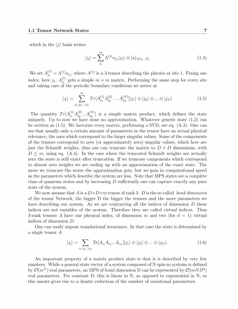
] is a simple matrix product, which defines the stateuniquely. Up to now we have done no approximation. Whatever generic state (1.2) canbe written as (1.5). We factorize every matrix, performing a SVD, see eq. (A.3). One cansee that usually only a certain amount of parameters in the tensor have an actual physicalrelevance, the ones which correspond to the larger singular values. Some of the componentsof the tensors correspond to zero (or approximately zero) singular values, which here arejust the Schmidt weights, thus one can truncate the matrix to D × D dimensions, withD ≤ m, using eq. (A.4). In the case where the truncated Schmidt weights are actuallyzero the state is still exact after truncation. If we truncate components which correspondto almost zero weights we are ending up with an approximation of the exact state. Themore we truncate the worse the approximation gets, but we gain in computational speedas the parameters which describe the system are less. Note that MPS states are a completeclass of quantum states and by increasing D sufficiently one can capture exactly any purestate of the system.
We now assume thatA is aD×D×m tensor of rank 3. D is the so called bond dimensionof the tensor Network, the bigger D the bigger the tensors and the more parameters wehave describing our system. As we are contracting all the indices of dimension D theseindices are not variables of the system. Therefore they are called virtual indices. Thus3-rank tensors A have one physical index, of dimension m and two (for d = 1) virtualindices of dimension D.
One can easily impose translational invariance. In that case the state is determined bya single tensor A
|χ〉 =∑
i1,i2...iN
Tr[Ai1Ai2 ...AiN ]|j1〉 ⊗ |j2〉 ⊗ ...⊗ |jN〉. (1.6)
An important property of a matrix product state is that it is described by very fewnumbers. While a general state vector of a system composed of N spin-m systems is definedby O(mN) real parameters, an MPS of bond dimension D can be represented by O(mND2)real parameters. For constant D, this is linear in N, as opposed to exponential in N, sothis ansatz gives rise to a drastic reduction of the number of variational parameters.
8 1. Theoretical Background
D1
D2
D3
D1<D2<D3
H
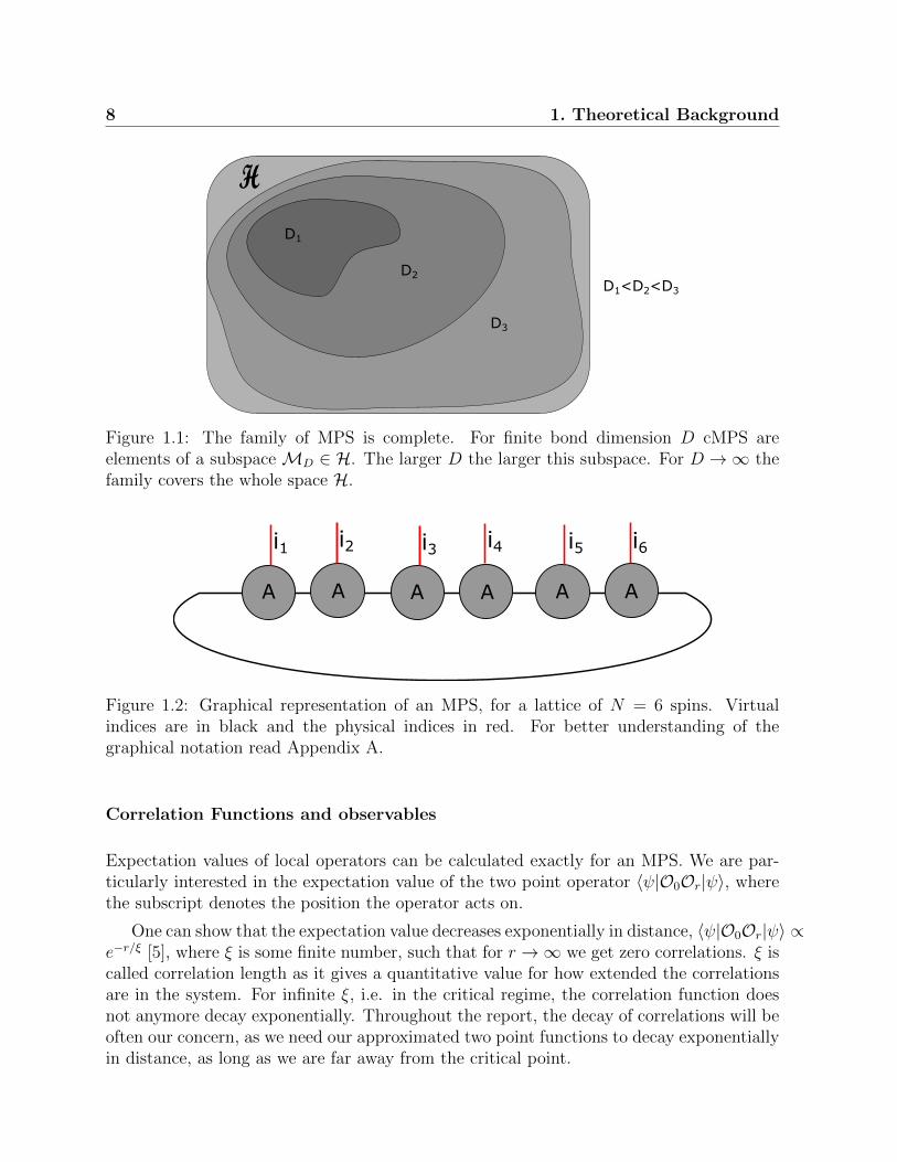
Figure 1.1: The family of MPS is complete. For finite bond dimension D cMPS areelements of a subspace MD ∈ H. The larger D the larger this subspace. For D →∞ thefamily covers the whole space H.
A A AA A A
i1 i2 i3 i4 i5 i6
Figure 1.2: Graphical representation of an MPS, for a lattice of N = 6 spins. Virtualindices are in black and the physical indices in red. For better understanding of thegraphical notation read Appendix A.
Correlation Functions and observables
Expectation values of local operators can be calculated exactly for an MPS. We are par-ticularly interested in the expectation value of the two point operator 〈ψ|O0Or|ψ〉, wherethe subscript denotes the position the operator acts on.
One can show that the expectation value decreases exponentially in distance, 〈ψ|O0Or|ψ〉 ∝e−r/ξ [5], where ξ is some finite number, such that for r →∞ we get zero correlations. ξ iscalled correlation length as it gives a quantitative value for how extended the correlationsare in the system. For infinite ξ, i.e. in the critical regime, the correlation function doesnot anymore decay exponentially. Throughout the report, the decay of correlations will beoften our concern, as we need our approximated two point functions to decay exponentiallyin distance, as long as we are far away from the critical point.

1.1 Tensor Network States 9
i j
Figure 1.3: Graphical representation of the expectation value of two operators, separatedby r = j − i sites. Taking expectation values corresponds to contracting the physicalindices.
1.1.2 Area Law
In this subsection the area law will be explained, as it is an important criterion for thephysical relevance of a state. There are many reasons to believe that states of a quantumsystem with an energy gap ∆E and a local Hamiltonian obey an area law [17, 16]. This non-generic property makes the physical quantum states to comprise only a small submanifoldHp ⊂ H, as for a generic state in H the entanglement entropy would grow with volume.
HHp
Figure 1.4: Observable states comprise only a tiny submanifold Hp ⊂ H, whose statesexhibit nongeneric properties.
Let us suppose we split a system in two parts B and its complement Bc, see Fig. 1.5.The entanglement entropy S is defined in respect to some bipartition as
S = −tr[ρB log2 ρB] (1.7)

10 1. Theoretical Background
where ρB = trBC [|ψ〉〈ψ|] is the reduced density matrix, |ψ〉 ∈ H. The entanglement entropymeasures the amount of entanglement between the two subsystems. It is zero if the stateρB is pure. If the to systems are entangled the reduced density matrix ρB correspondsto a mixed state. Now the area law states that the entanglement entropy grows at mostproportionally with the boundary ∂B between the two partitions, so Smax ∝ |∂B|.
Bc
B
Figure 1.5: Bipartite system
Matrix Product states are a family of states which satisfy the area law. In one dimensionthe boundary of the subsystem consists of two sites independent of the particle numberN , see Fig.1.6. One can show that the entanglement entropy of an MPS is bounded bySmax = O(log2(D)), where D is the bond dimension of the tensors. That means that
A A AA A A A A AA A A
Figure 1.6: Bipartition of an MPS
the bound is independent of the system size. The behaviour of the entanglement scalingis therefore the same for MPS as for ground states of gapped models. Moreover, thebond dimension turns out to be a quantitative measure of the entanglement present inthe quantum state. For example for D = 1 we have a separable product state, so all theparticles are independent, whereas D > 1 provides non trivial entanglement properties.
A question which may arise is how well an MPS approximates a naturally occurringstate. It was shown by Hastings [27] the error in approximating the ground state by amatrix product state of bond dimension D scales as D−1/ξ, where ξ is the correlationlength. For a finite ξ the approximation gets better when we increase D. Moreover, theapproximation works well when ξ is small, so for short range correlations, which arisefrom finite, local Hamiltonians. As one reaches the critical point, i.e. the gap is closingand the correlation length is exploding, the MPS is not anymore describing the system as
1.1 Tensor Network States 11
efficiently. Thus, for ∆E → 0 we need higher bond dimensions to compensate. We will seean illustration of this later.
1.1.3 Projected Entangled Pairs State (PEPS)
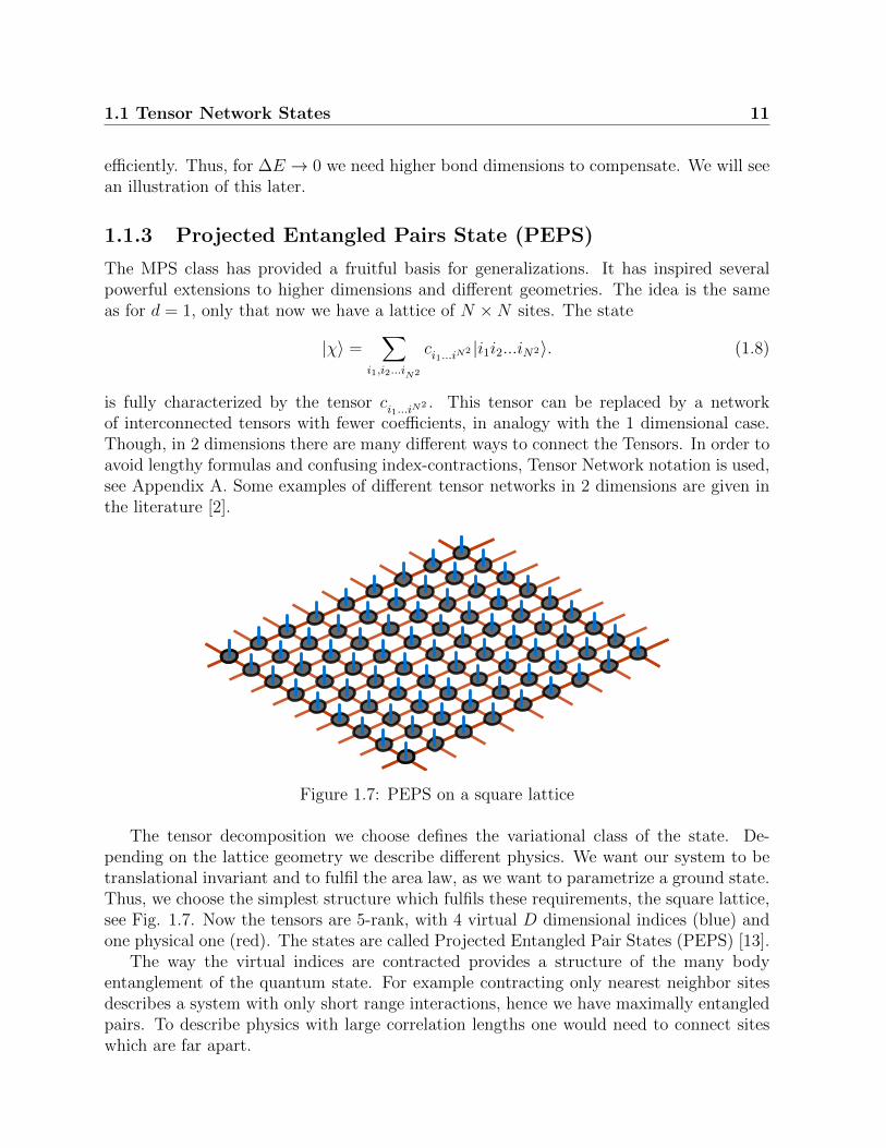
The MPS class has provided a fruitful basis for generalizations. It has inspired severalpowerful extensions to higher dimensions and different geometries. The idea is the sameas for d = 1, only that now we have a lattice of N ×N sites. The state
|χ〉 =∑
i1,i2...iN2
ci1...iN2 |i1i2...iN2〉. (1.8)
is fully characterized by the tensor ci1...iN2 . This tensor can be replaced by a networkof interconnected tensors with fewer coefficients, in analogy with the 1 dimensional case.Though, in 2 dimensions there are many different ways to connect the Tensors. In order toavoid lengthy formulas and confusing index-contractions, Tensor Network notation is used,see Appendix A. Some examples of different tensor networks in 2 dimensions are given inthe literature [2].
Figure 1.7: PEPS on a square lattice
The tensor decomposition we choose defines the variational class of the state. De-pending on the lattice geometry we describe different physics. We want our system to betranslational invariant and to fulfil the area law, as we want to parametrize a ground state.Thus, we choose the simplest structure which fulfils these requirements, the square lattice,see Fig. 1.7. Now the tensors are 5-rank, with 4 virtual D dimensional indices (blue) andone physical one (red). The states are called Projected Entangled Pair States (PEPS) [13].
The way the virtual indices are contracted provides a structure of the many bodyentanglement of the quantum state. For example contracting only nearest neighbor sitesdescribes a system with only short range interactions, hence we have maximally entangledpairs. To describe physics with large correlation lengths one would need to connect siteswhich are far apart.
12 1. Theoretical Background
There are many specific examples of non-trivial problems that have been solved exactlyby PEPS, such as the Toric Code model, the 2d Resonating Valence Bond State, the 2dAKLT state and the 2d cluster state [1].
Thus, Tensor Network states are mathematical representations of quantum many-bodystates fully characterized by a Tensor Network. The individual tensors encode the keyproperties of the overall wavefunction and the Tensor Network geometry is based on theentanglement structure of the system. The symmetries of the physical system imposesymmetries on the tensors.
So far, everything in this report has been restricted to the lattice setting. To studycontinuous quantum system with these tools one would discretize the space and make useof a variational method on the lattice. The goal of the next two sections is to explainhow to avoid the discretization and how to apply these variational methods directly in thecontinuum.
1.2 Continuous Matrix Product States (cMPS)
An important challenge is the generalization of Tensor Networks from lattice to contin-uous systems, which would allow the direct study of quantum field theories. The ansatzformulated in the continuum would not require an underlying lattice approximation. Thisis useful because the continuum provides a whole range of exact and approximate analytictechniques, as Gaussian functional integrals. In the continuum the states are called con-tinuous Matrix Product states (cMPS), and in analogy with the standard MPS they areexpected to be both an computationally efficient and complete set of states.
We consider a one dimensional system of bosons with periodic boundary conditions, as-sociated with field operators ψ(x) ∈ H with canonical commutation relations, [ψ(x), ψ†(y)] =δ(x − y) and 0 ≤ x, y ≤ L continuous space coordinates. |Ω〉 is the vacuum state of thephysical Hilbert space H, with ψ(x)|Ω〉 = 0 for ∀x ∈ [0, L]. The complete family of cMPSis defined as [18]:
|χ〉 = Traux[Pe∫ L0 dx[Q(x)⊗1+R(x)⊗ψ†(x)]]|Ω〉 (1.9)
with Q(x), R(x) position dependent complex D×D matrices, that act on a D dimensionalauxiliary space Haux ∈ CD, Traux the trace over the auxiliary system. We will see that Dcorresponds to the bond dimension we have seen in the discrete case. In a translationalinvariant system Q and R do not depend on the position. Pexp is the path orderedexponential, which will be explained in the next paragraph. The Langrangian L(x) =[Q(x)⊗ 1 +R(x)⊗ ψ†(x)], has to be invariant under the symmetries of the system.
We try to gain some intuition into what these states describe, by discretizing the spaceand stressing the meaning of the sites at which a particle is created. First, we split the space[0, L] into N equal length ε paths. The path-ordered exponential appearing in eq.(1.9) isthen simply
Pe∫ L0 dxL(x) = lim
ε→0
[eεL(uN )eεL(uN−1)...eεL(u1)
],
where uj is the position of site j = 1, 2 . . . N . Next, we expand eεS(x) and get

1.2 Continuous Matrix Product States (cMPS) 13
1 NFigure 1.8: Partition in N sites. Example case for n=2, such that |χ〉 =
Traux[limε→0Pe∫ xNx11
Q(x)dxeεR(x11)⊗ψ(x11)Pe
∫ x11x6
Q(x)dxeεR(x6)⊗ψ(x6)Pe
∫ x60 Q(x)dx|Ω〉
|χ〉 =∞∑n=0
∫0<x1<x2<...<xn<L
dx1dx2...dxnφnψ†(x1)ψ†(x2)...ψ†(xn)|Ω〉 (1.10)
where n is the particle number and xi the positions of the particles with i = 1, 2 . . . n ,which of course coincide with some of the uj. The wavefunction is given by
φn = Traux[uQ(0, x1)R(x1)uQ(x1, x2)R(x2)...R(xn)u(xn, L)] (1.11)
where uQ(x, y) = P exp[∫ yxQ(x)dx]. Equation (1.10) shows that an MPS can be interpreted
as a superposition over the different particle number sectors in the Fock space. uQ can beinterpreted as a propagator, while R can be understood as a scattering matrix that createsa physical particle.
To make that more explicit for the reader we compute the wave function representationin an example case, for two particles n = 2 distributed on a lattice of N sites, see Fig.1.8.In this specific case where the positions of the particles is fixed the state gets
|χ(x1 = u6, x2 = u11)〉n=2 = Traux[limε→0Pe
∫ xNx11
Q(x)dxeεR(x11)⊗ψ(x11)
Pe∫ x11x6
Q(x)dxeεR(x6)⊗ψ(x6)Pe
∫ x60 Q(x)dx|Ω〉,
but of course in order to get the most generic state with two particles one has to integrateover the positions |χ〉n=2 =
∫dx1dx2|χ(x1, x2)〉n=2.
1.2.1 Correlation functions and expectation values
We are interested in computing some expectation values of normal ordered observables〈χ(Q,R)| : O[ψ†, ψ] : |χ(Q,R)〉, particularly the correlation function and the energy.As the states themselves depend on the matrices Q and R, so will the observables. As weare in a Field Theory the easiest way usually is proceeding by using a generating functional
Z[J, J] = Tr
[eLTP exp
∫ L/2
−L/2dxJ(x)[R⊗ 1D] + J(x)[1D ⊗R]
](1.12)
where T = Q⊗1D+1D⊗Q+R⊗R is coming from the fact that the state is not normalized.Now we compute the two point function,
〈χ(Q,R)|ψ†(x)ψ(y)|χ(Q,R)〉 =δ
δJ(y)
δ
δJ(x)Z[J, J]|j.J=0 (1.13)

14 1. Theoretical Background
which simply, for x < y, takes the form
〈χ(Q,R)|ψ†(x)ψ(y)|χ(Q,R)〉 = Tr[e(x+L/2)T(R⊗ 1D)Pe(y−x)T(1D ⊗R)Pe(L/2−y)T
]One can check that the real part of the eigenvalues of T, is finite and non positive. Thus, forgrowing distance |x−y| the exponential e(y−x)T is decreasing exponentially. The realizationthat the correlation function is decreasing exponentially with distance is essential, for theMPS to describe efficiently a system of a gapped Hamiltonian. On the other hand, it isimpossible to describe a system at the critical point.
The density operator at point x is given by
〈χ(Q,R)|ψ†(x)ψ(x)|χ(Q,R)〉 = Tr[eLT(R⊗R)] (1.14)
To compute the energy one needs to take the expectation value of the Hamiltonian
E = 〈H〉 = 〈T 〉+ 〈V 〉 (1.15)
where 〈T 〉 = 〈χ(Q,R)|(ddxψ†(x)
) (ddxψ(x)
)|χ(Q,R)〉 is the kinetic energy and 〈V 〉 the
interaction energy. The last term can contain the density operator of eq.(1.14), or higherorder interactions, expressed in terms of higher order moments. For example, a four point
interaction term could be V =∫ L/2−L/2 v(x−y)ψ†(x)ψ†(y)ψ(y)ψ(x) and one needs to compute
begineqnarray
〈χ(Q,R)|V |χ(Q,R)〉 = 〈χ(Q,R)|ψ†(x)ψ†(y)ψ(y)ψ(x)|χ(Q,R)〉. (1.16)
That way, one finds the variational value of the energy E = E(Q,R). Note that no furtherapproximation has been done.
1.2.2 Link with discrete MPS
Now we will show how these continuous MPS can be understood as a limit of a familyof discrete MPS. Again we consider a tranlational invariant system of bosons of lengthL with periodic boundary conditions. We approximate the continuum [−L/2, L/2] by alattice with spacing ε and N = L/ε sites. We reconstruct the continuum by taking ε→ 0.On every site we can create and annihilate particles with the creation and annihilationoperators a†i and ai, which fulfill the commutation relation [ai, a
†j] = δij. We can relate
them to the field operators ψ(x) by
an =
∫ (n+1)ε
nε
ψ(x)dx (1.17)
and its hermitian conjugate. The field operators need to satisfy the commutation relation[ψ(x), ψ†(y)] = δ(x− y). If we define a rescaled annihilation operator ψi as
ψi =√εai (1.18)

1.2 Continuous Matrix Product States (cMPS) 15
which fulfils
[ψi, ψ†j ] =
δijε
(1.19)
in the limit ε → 0 we regain ψi → ψ(x). Now we can define a family of translationalinvariant MPS on a discretized lattice as
|χε〉 =∑i1...iN
Tr[Ai1 ...AiN ](ψ†1)i1 ...(ψ†N)iN |Ω〉. (1.20)
This is the same state as defined in eq.(1.6), for |jl〉 = (ψ†l )jl ||Ω〉. We will take ε→ 0 and
n → ∞ such that the particle density ρ stays constant. Under this condition it is highlyunlikely for two particles to be at the same point. Thus we will make the assumption thati = 0 or 1. We choose the matrices A = A(Q,R) to depend on the matrices R and Q, insuch a way that as ε→ 0 the limit of the state is well defined and we get the cMPS of eq.(1.10):
A0 = 1 + εQ (1.21)
A1 = εR (1.22)
An = εnRn
n!, (1.23)
We are in the special case where we restrict to a finite particle density, most of the sitesare empty in the limit and A0 is the dominant matrix.
The correspondence of cMPS with MPS is important, because they most likely inheritall the properties of an MPS, like the fact that the entanglement entropy is bounded fromabove by 2log2(D), see sec.1.1.2.
1.2.3 Application on the Lieb-Liniger Model
The cMPS have been successfully used as a variational ansatz for strongly correlated con-tinuous theories, for example to find the ground state energy of the Lieb-Liniger model[28], which describes non relativistic bosons in an one dimensional space interacting via acontact potential
H =
∫ ∞−∞
[dψ†
dx
dψ
dx+ cψ†(x)ψ†(x)ψ(x)ψ(x)
]. (1.24)
The goal was to approximate the ground state energy density by variational methods usingMPS and compare it with the exact analytical solution and Monte Carlo algorithms [18].For the first we need to use the expressions 〈ψψ〉 computed in section 1.2.1. As the systemis solvable analytically, using the Bethe Ansatz, a comparison is possible. The energydensity is finite and can be expressed as ρ3e(c/ρ), where ρ is the density and e(c/ρ) theenergy density at ρ = 1. For c = 2 the Bethe ansatz gives e = 1.0504 and the MonteCarlo Method e = 1.0518. With the cMPS variational method one obtains a differentenergy density for different bond dimensions. One expects the method to approximate theactual lowest energy state better for bigger bond dimensions, thus the actual lowest energy
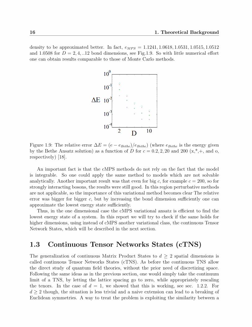
16 1. Theoretical Background
density to be approximated better. In fact, eMPS = 1.1241, 1.0618, 1.0531, 1.0515, 1.0512and 1.0508 for D = 2, 4, ..12 bond dimensions, see Fig.1.9. So with little numerical effortone can obtain results comparable to those of Monte Carlo methods.
Figure 1.9: The relative error ∆E = (e− eBethe)/eBethe) (where eBethe is the energy givenby the Bethe Ansatz solution) as a function of D for c = 0.2, 2, 20 and 200 (x,*,+, and o,respectively) [18].
An important fact is that the cMPS methods do not rely on the fact that the modelis integrable. So one could apply the same method to models which are not solvableanalytically. Another important result was that even for big c, for example c = 200, so forstrongly interacting bosons, the results were still good. In this region perturbative methodsare not applicable, so the importance of this variational method becomes clear The relativeerror was bigger for bigger c, but by increasing the bond dimension sufficiently one canapproximate the lowest energy state sufficiently.
Thus, in the one dimensional case the cMPS variational ansatz is efficient to find thelowest energy state of a system. In this report we will try to check if the same holds forhigher dimensions, using instead of cMPS another variational class, the continuous TensorNetwork States, which will be described in the next section.
1.3 Continuous Tensor Networks States (cTNS)
The generalization of continuous Matrix Product States to d ≥ 2 spatial dimensions iscalled continuous Tensor Networks States (cTNS). As before the continuous TNS allowthe direct study of quantum field theories, without the prior need of discretizing space.Following the same ideas as in the previous section, one would simply take the continuumlimit of a TNS, by letting the lattice spacing go to zero, while appropriately rescalingthe tenors. In the case of d = 1, we showed that this is working, see sec. 1.2.2. Ford ≥ 2 though, the situation is less trivial and a naive extension can lead to a breaking ofEuclidean symmetries. A way to treat the problem is exploiting the similarity between a

1.3 Continuous Tensor Networks States (cTNS) 17
tensor contraction over the indices lying on the links of a tensor network and a functionalintegral over a field living on the continuum limit of this construction, as explained inAppendix B.
We begin with the definition of a cTNS for bosonic quantum fields in the functionalintegral formulation, as it is defined in [22]:
|V, a〉 =
∫Dφ exp
(−∫
Ω
ddx1
2
D∑k=1
[∇φk(x)]2 + V [φ(x)]− a[φ(x)]ψ†(x)
)|0〉 (1.25)
The state describes bosons in d spacial dimensions and periodic boundary conditions. Thephysical Fock vacuum state is noted as |0〉. We have two sorts of field operators, thephysical bosonic ones, which fulfil the commutation relation [ψ(x), ψ†(y)] = δd(x− y) andthe auxiliary fields, which are D dimensional vectors, φ = φkDk=1, being integrated overin the path integral. D is the continuous equivalent of bond dimensions, and is calledbond-field dimension. Here, we choose a and V such that they do not depend explicitly onthe position, since we restrict ourselves to translational invariant systems.
auxiliary field
physical field
auxiliary degrees of fredom
physical degrees of fredom
Figure 1.10: Functional integral representation – In the discrete (left) a tensor networkstate is obtained from a contraction of auxiliary indices connecting the elementary tensorswith each other and with a boundary tensor. In the continuum (right), the contraction isreplaced by a functional integral and the auxiliary indices by fields φ. [22]
To gain some physical understanding of these states it is convenient to express them asa generalization of bosonic field coherent states
|V, a〉 =
∫dµ(φ)AV (φ)|a(φ)〉 (1.26)
where
|a(φ)〉 = exp
(∫Ω
ddxa[φ(x)]ψ†(x)
)|0〉 (1.27)
18 1. Theoretical Background
is the unnormalized field coherent state, which specifies the occupation number of theparticles in FOck space,
AV (φ) = exp
(−∫
Ω
ddxV [φ(x)]
)(1.28)
a complex amplitude and
dµ(φ) = Dφ exp
[−1
2
∫Ω
D∑k=1
[∇φ(x)]2
](1.29)
the massless free probability measure of the auxiliary field. For a constant auxiliary fieldφ(x) = φ the cTNS simplifies to a simple bosonic coherent state. That is the case when Ais nonzero only for one mode. The measure dµ(φ) suppresses the large momentum modesand the amplitude term is bigger in the regions the potential is smaller. In case the fieldis massless, we get A = 1.
1.3.1 Correlation functions and expectation values
Just as in Section 1.2.1 we are interested in computing observables, as the correlationfunctions and the energy of a given Hamiltonian. In order to compute them, we firstintroduce the generating functionals
Zj′,j =〈V, a| exp(
∫ddxj′(x) · ψ†(x) exp(
∫ddyj(y) · ψ(y))|V, a〉
〈V, a|V, a〉(1.30)
which we use to compute the two point functions
〈ψ†(x)ψ(y)〉 =δ
δj′(x)
δ
δj(y)Zj′,j|j′,j=0, (1.31)
〈ψ(x)ψ(y)〉 =δ
δj(x)
δ
δj(y)Zj′,j|j′,j=0 (1.32)
and
〈ψ†(x)ψ†(y)〉 =δ
δj′(x)
δ
δj′(y)Zj′,j|j′,j=0. (1.33)
but one can take higher order functional derivatives to obtain higher order momenta, likefour point functions.
We expect the two point function 〈ψ†(x)ψ(y)〉 to decay exponentially in distance and〈ψ†(x)ψ(x)〉 to be positive and finite as it expresses the density of the particles at positionx, but we will come back to that when we actually perform the computations in the twonext Chapters of this report.
For a given Hamiltonian H we can compute the energy as a function of V and a.To do so we express it as E = 〈H〉 = 〈T 〉 + 〈V 〉, where the interaction operator can
1.3 Continuous Tensor Networks States (cTNS) 19
include terms of the form 〈ψ†(x)ψ(x)〉, 〈ψ†(x)ψ†(x)〉, 〈ψ(x)ψ(x)〉 (two point functions)and 〈ψ†(x)ψ†(y)ψ(y)ψ(x)〉 (four point function) or higher. Of course 〈V 〉 ∈ R, as it is aphysical observable. The kinetic term is 〈T 〉 = 〈
(ddxψ†(x)
) (ddxψ(x)
)〉 ∈ R. For models
which are known to have finite energy densities it is important that the expression we getfor E(V, a) is finite too. Note that all the expectation values so far have been expressed inreal space.
To compute the generating functional one uses the Baker-Campell- Hausdorf formula.We obtain
Zj′,j =1
N
∫dµ(φ′)dµ(φ)× e
∫Ω V∗[φ′(x)]+V [φ(x)]−a∗[φ(x)]·a[φ(x)]−j·a[φ(x)]−j′·a[φ′(x)] (1.34)
where N = 〈V, a|V, a〉 and dµ(φ) is given in (1.29). This integral is solvable analyticallyonly if it is gaussian. That restricts the form of the functions V and a for our applications.We will have to choose them such that the last integral is at most quadratic in φ. Alreadyin this case we will see that the computations are quite tideous.
1.3.2 Restriction to Gaussian cTNS (GCTNS)
In our applications we will consider only a subclass of the cTNS, with which we can computethe closed formulas of expectation values: the Gaussian continuous Tensor Network States(GCTNS), see Fig.1.11. A TNS is Gaussian if it is at most second order in φ. In this casethe most general form the functions V [φ(x)] and a[φ(x)] can have are respectively
V [φ(x)] = V (0) + V(1)k φk + V
(2)kl φkφl, (1.35)
a[φ(x)] = a(0) + a(1)k φk, (1.36)
where Einstein summation is implied. We will simplify even more taking
a(0) = V (1) = 0 (1.37)
and for simplicity we will write a(1) = a, and V (2) = V so the generic form of the GCTNSin the functional integral representation is
|V, a〉 =
∫Dφexp
∫ddx(−1
2)φ(x)(−∇2 + V )φ(x) + a(x)φ(x)ψ†(x)
|0〉. (1.38)
where V is a D×D dimensional matrix and a is a D dimensional vector. When integratingout the φ field it becomes obvious why this state is Gaussian
|V, a〉 ∝ exp
∫ddxddy
1
2ψ†(x)aT (−∇2 + V )−1(x− y)aψ†(y)
|0〉. (1.39)
One can check that if one takes higher order terms in a or V the generating functional(1.34) will include φ3 or even higher order terms in the exponential. But it is impossible

20 1. Theoretical Background
to solve a non gaussian integral. Thus, if we take non gaussian cTNS we cannot computethe closed form of the expectation values, which are essential for our method.
We will use this parametrization to approximate the ground state of a given Hamil-tonian. But let us first discuss wheather a Gaussian state is a good approximation. Weknow that for Hamiltonians which are at most quadratic in the creation and annihilationoperators, the ground state is a Gaussian State. But for more generic Hamiltonians theground state does not have to be Gaussian. However, in some cases a Gaussian state isstill some good approximation of the actual ground state [33].
H
cTNSgTNS MM
Figure 1.11: For a finite D the manifold of cTNS McTNS is a subspace of the full Hilbertspace H, and the space of GCTNS MGCTNS is a subspace of McTNS.

Chapter 2
Algorithm and AnalyticComputations
In this chapter we will work exclusively with Gaussian continuous Tensor Network States.The goal is to compute the analytic closed forms of expectation values and their derivatives,which we need in order to implement the variational algorithm explained below.
2.1 Algorithm
So let us first understand what the algorithm is computing. It optimizes the variationalparameters of our state such that we arrive at the lowest energy state, within our parametricclass.
Essential for applying the variational method [24] is to guess a trial wavefunction for theproblem, which has adjustable parameters called variational parameters. These parametersare varied until the energy of the trial wavefunction is minimized. The resulting trialwavefunction and its corresponding energy are variational approximations to the exactwavefunction and energy. In particular, the variational principle asserts that for any state|ψ〉 in the Hilbert space H of a system with Hamiltonian H one finds an energy expectationvalue that exceeds the ground state energy,
ε0 ≤〈ψ|H|ψ〉〈ψ|ψ〉
, (2.1)
with ε0 the ground state energy of H. If one has a variational ansatz states |ψ(z)〉, withz being the variational parameter, we try to find the value of the parameter z such that|ψ(z∗)〉 gives the lowest energy E0 ≥ ε0.
Now we need to choose an efficient method in order to get the correct parameter values.One could compute them analytically in a simple problem, by simply looking for the minimaof the energy function w.r.t. the parameters. But in most cases it is too hard, especially forbig D. Numerically the easiest way to solve the problem is with some variational algorithm.There are many efficient algorithms known to solve these sort of problems, but the main

22 2. Algorithm and Analytic Computations
idea can be captured with a simple gradient descent method. The gradient descent methodis a first order iterative optimization algorithm to find the minimum of a function. In everyiteration the algorithm optimizes the value of the parameters following the descent of thefunction to optimize.
In our case this function is the energy, E = 〈V, a|H|V, a〉. The variational parametersare the coefficients of the matrix V and the vector a. Let us suppose that x is a 4D vectorwith components all the parameters of out state |V, a〉. The equation which states how theparameter xb is changing in one step is given by
xbn+1 = xbn − rdE
dxb
where r i the iteration step and we compute
dE
dxb=
d
dxb〈V, a|h|V, a〉 − E d
dxb〈V, a|V, a〉
Note that the second term comes from the fact that our state |V, a〉 is unnormalized,〈V, a|V, a〉 6= 1. We get
xbn+1 = xbn −(
d
dxb〈V, a|h|V, a〉 − E d
dxb〈V, a|V, a〉
). (2.2)
In order to implement the algorithm one needs to know the closed formula for E, dEdxb
andddxb〈V, a|V, a〉, as a function of the parameters xb.As already seen in Section 1.3.1 we can express the energy function as a sum over
different expectation values. The terms which might be included in the energy functioncan be very complicated, so we will restrict ourselves to compute only the ones we willneed later on for our toy models, see Chapter 3, which will be 〈ψ†(x)ψ(x)〉, 〈ψ(x)ψ(x)〉 and〈ψ†(x)ψ†(x)〉 for the interaction part and ∂2
x〈ψ†(x)ψ(x)〉 for the kinetic term. Subsequently,we will compute their derivatives with respect to the variational parameters. Having themwe know the analytic form of dE
dxb. In the end of this section we compute d
dxb〈V, a|V, a〉. All
of these expressions are used to implement the variational code.
2.2 Correlation functions for GCTNS
In this section we compute the analytic closed forms of the two point functions, by usingthe generating functionals. Will will need to compute them as integrals over the momenta,
〈ψ†(x)ψ(x)〉 =∫
ddp(2π)d〈ψ†pψp〉eip(x−y). At this point the dimensions d of the problem become
relevant and one needs to check that the quantities are finite.The generating functional from the GCTNS (1.30) is
Zj′,j =1
Nexp
∫ddxddy
1
2Λ(j, j′)T (x) ·K(x, y) · Λ(j, j′)(y), (2.3)

2.2 Correlation functions for GCTNS 23
where
Λ(j, j′) =
(V − ajV − a∗j′
)(2.4)
and
K(x− y)
[−∇2 + V −a⊗ a∗−a∗ ⊗ a −∇2 + V
]= 12D×2Dδ(x− y) (2.5)
Using the fact that the auxiliary system is translation invariant we write K(x, y) =K(x− y), which can be written in Fourrier space
K(x− y) =1
(2π)d
∫ddpK(p)eip(x−y)
with
K(p) =1
(2π)d
[p2 + V −a⊗ a∗−a∗ ⊗ a p2 + V
]−1
=1
(2π)dM−1(p) (2.6)
Using (1.31), (1.32) and (1.33) we get the expressions for the two point functions as func-tions of V and a:
〈ψ†(x)ψ(y)〉 =1
2
∫ddp
(2π)daTK(p)a∗eip(x−y) + a∗TK(p)aeip(x−y), (2.7)
〈ψ(x)ψ(y)〉 =
∫ddp
(2π)daTK(p)aeip(x−y) (2.8)
and
〈ψ†(x)ψ†(y)〉 =
∫ddp
(2π)da∗TK(p)a∗eip(x−y). (2.9)
withaT =
(a1 a2 ... aD 0 0 0 ... 0
), (2.10)
aT∗ =(0 0 0 ... 0 a∗1 a∗2 ... a∗D
). (2.11)
Note that a is a 2D dimensional vector now, it is not the same as a.At this point it is important to check if the correlation function C(x−y) = 〈ψ†(x)ψ(y)〉
is decaying exponentially. As seen in the discrete case and for cMPS, this is an importantproperty of states which describe non critical, local hamiltonians. The matrix K(p) con-tains elements which are polynomials in p. The terms aTK(p)a∗eip(x−y) are of the form
A(p2+B)n
, with n = 1, 2 . . . 2D. Their fourier transform is proportional to e−√B|x−y|. Thus,
the correlation function decays exponentially with distance.One can also derive the correlation functions directly in momentum space. Then, the
general form of the generating functional is
Zj′,j =〈V, a| exp(
∫ddp
(2π)dj′(p) · ψ†(p) exp(
∫ddp
(2π)dj(−p) · ψ(p))|V, a〉
〈V, a|V, a〉(2.12)
24 2. Algorithm and Analytic Computations
which for GCTNS in a translation invariant system gets
Zj′,j =1
Nexp
∫ddp
(2π)d1
2Λ(j, j′)T (p) ·K(p) · Λ(j, j′)(−p). (2.13)
The correlation functions in momentum space are given by
〈ψ†pψp′〉 =∂2Z
∂j′(p)∂j(−p′)=
1
2
(aTK(p)a∗ + a∗TK(p)a
)δ(p− p′) (2.14)
〈ψpψp′〉 =∂2Z
∂j(−p)∂j(−p′)= (aTK(p)a)δ(p+ p′) (2.15)
〈ψ†pψ†p′〉 =
∂2Z
∂j′(p)∂j′(p′)= (a∗TK(p)a∗)δ(p+ p′) (2.16)
As for the four-point function, using Wicks Theorem we can write it as combinations ofthe two point functions
〈ψ†p−qψ†k+qψkψp〉
= 〈ψ†p−qψ†k+q〉〈ψkψp〉+ 〈ψ†p−qψk〉〈ψ
†k+qψp〉+ 〈ψ†p−qψp〉〈ψ
†k+qψk〉
= 〈ψ†−k−qψ†k+q〉〈ψkψ−k〉+ 〈ψ†kψk〉〈ψ
†k+qψk+q〉+ 〈ψ†pψp〉〈ψ
†kψk〉 (2.17)
2.2.1 Closed form of the correlation functions
In order to implement the algorithm we need to compute the closed form of the correlationfunctions in real space 〈ψ(†)(x)ψ(†)(x)〉 of eq.(2.7)-(2.9), which means we need to performthe integration. We know the analytic form of K(p) from eq. (2.6) and now we needperform the integral over the momenta. First we diagonalize matrix K(p) by diagonalizingM(p) = p2 · 1 + U−1ΛU so we get
K(p) =1
(2π)dU−1(p2 · 1 + Λ)−1U, (2.18)
where Λ is a 2D × 2D diagonal matrix with eigenvalues λ1, λ2, ..., λ2D and U is a unitary2D × 2D matrix. M(p) needs to be positive definite matrix, for the state to be physical,thus Re[λi] > 0. The correlation function, at equal points, from (2.8) writes
〈ψ(x)ψ(x)〉 =
∫ddp
(2π)d(aT · U)(p2 · 1 + Λ)−1(U−1 · a) =
1
(2π)d
2D∑i
(aT · U)i(U−1 · a)iI1(λi)
(2.19)where
I1(λi) =
∫ddp
(2π)d1
p2 + λi
2.3 Computation of derivatives 25
is an integral computed in the Appendix C. Similarly, the other correlation functions write
〈ψ†(x)ψ(x)〉 =
[2D∑i
(a∗T · U)i(U−1 · a)i + (aT · U)i(U
−1 · a∗)i
]I1(λi) (2.20)
and
〈ψ†(x)ψ†(x)〉 =2D∑i
(a∗T · U)i(U−1 · a∗)iI1(λi). (2.21)
For the kinetic term in the Hamiltonian we need the derivative of the correlation function
limx→y
∂x∂y〈ψ†(x)ψ(y)〉 =
[2D∑i
(a∗T · U)i(U−1 · a)i + (aT · U)i(U
−1 · a∗)i
]I1kin(λi) (2.22)
where
I1kin(λi) =
∫d2p
(2π)2
p2
p2 + λi
is computed in Appendix C.
2.3 Computation of derivatives
2.3.1 Derivatives of correlation functions
To implement the algorithm (2.2) we need the derivative of the energy ddxb〈V, a|H|V, a〉,
where x is a vector of all the real parameters which describe our state, and b = 1, . . . 4D.That means we need to compute the derivatives of the correlation functions and of thekinetic term.
We start with the derivatives ∂∂xb〈ψ(†)(x)ψ(†)(y)〉. The derivation is similar for all of
them, so we just will show the derivation steps for one. We take the derivative of eq. (2.8)
∂
∂xb〈ψ(x)ψ(y)〉 =
∫ddp
(2π)daT · ∂K(p)
∂xb· aeip(x−y) (2.23)
where K(p) = 1(2π)d
M−1(p), from eq. (2.6). Using M−1M −MM−1 = 0, we get that
∂M−1
∂xb= −M−1∂M
∂xbM−1 (2.24)
For different variational parameters we get different analytical formulas. The differentforms of the derivative dM−1
dxbare computed below:
∂M
∂Re(Vii)= ei · eTi + ei+d · eTi+d
26 2. Algorithm and Analytic Computations
and∂M
∂Im(Vii)= ei · eTi − ei+d · eTi+d
where ei the 2D unit vector with only nonzero element the ith component. Also,
∂M
∂Re(aj)= −[ej · a∗T + a∗ · eTj + ej+d · aT + a · eTj+d]
∂M
∂Im(aj)= −i[ej · a∗T + a∗ · eTj − ej+d · aT − a · eTj+d]
We want to perform the integral over the momenta, so again, we diagonalize M(p) =p2 · 1 + U−1ΛU by using the unitary matrix U such that
−aTM−1∂M
∂xbM−1a = −(aTU)U−1M−1UU−1∂M
∂xbUU−1M−1U(U−1a) (2.25)
Combining everything we arrive at the closed formulas. In particular, for the parametersRe[Vii], Im[Vii] we get
∂
∂Re[Vij]〈ψ(x)ψ(y)〉 =
2d∑lk
(aTU)lC+lk(U
−1a)kI2(λl, λk),
∂
∂Im[Vij]〈ψ(x)ψ(y)〉 = i
2d∑lk
(aTU)lC−lk(U
−1a)kI2(λl, λk).
and for the slightly more complicated two point function 〈ψ†(x)ψ(x)〉, we proceed similarlyand get
∂
∂Re[Vij]〈ψ†(x)ψ(y)〉 = −
2d∑lk
1
2[(aTU)lC
+lk(U
−1a∗)k + (a∗TU)lC+lk(U
−1a)k]I2(λl, λk)
∂
∂Im[Vij]〈ψ†(x)ψ(y)〉 = −i
2d∑lk
1
2[(aTU)lC
−lk(U
−1a∗) + (a∗TU)lC−lk(U
−1a)k]I2(λl, λk)
whereC±lk = −(U−1
li Uik ± U−1l,i+dUi+d,k)
The integral
I2(λk, λl) =
∫ddp
(2π)d1
p2 + λk
1
p2 + λleip(x−y)
is computed in Appendix C.In analogy, for the parameters Re[aj], Im[aj] we compute
∂
∂Re[aj]〈ψ(x)ψ(y)〉 =
2d∑i
GijI1(λi) +2d∑ik
FRijkI2(λi, λk)
2.3 Computation of derivatives 27
and∂
∂Im[aj]〈ψ(x)ψ(y)〉 = i
∑i
GijI1(λi) +∑ik
F IijkI2(λi, λk)
with
Gij = [Uji(U−1a)i + (aTU)iUij].
We use
FRijk = −(aTU)i(U
−1 ∂M
∂Re(aj)U)ik(U
−1a)k,
F Iijk = −(aTU)i(U
−1 ∂M
∂Im(aj)U)ik(U
−1a)k
Also, in the case of 〈ψ†(x)ψ(x)〉 we obtain the following the derivatives in closed form
∂
∂Re[aj]〈ψ†(x)ψ(y)〉 =
2d∑i
G+ijI1(λi) +
∑i,k
F+ijkI2(λi, λk) (2.26)
and
∂
∂Im[aj]〈ψ†(x)ψ(y)〉 = i
∑i
G−(ψ†ψ, i, j)I1(λi) + i∑i,k
F−(ψ†ψ, i, j, k)I2(λi, λk),
where
G+ij = Uji(U
−1a∗)i + (aTU)iU−1i,j+d + (a∗TU)iU
−1ij + Uj+d,i(U
−1a)i,
G−ij = Uji(U−1a∗)i − (aTU)iUij+d − Uj+di(U−1a)i + (a∗TU)iUij
and
F+ijk = −[(aTU)i(U
−1a∗)k + (a∗TU)i(U−1a)k](U
−1 ∂M
∂Re(aj)U)ik,
F−ijk = −[(aTU)i(U−1a∗)k + (a∗TU)i(U
−1a)k](U−1 ∂M
∂Im(aj)U)ik
For the kinetic terms, for example limx→yd
dRe[Vij ]∂x∂y〈ψ†(x)ψ(y)〉 we just need to replace
the integrals of each form by their kinetic integrals, i.e. replace I2 by I2kin, see AppendixC.
Now we have all the ingredients to compute the derivative of the energy.
2.3.2 Derivatives of the norm
In this subsection the derivative of the norm we use in eq.(2.2) is computed
∂
∂xb〈V, a|V, a〉 =
∂〈V, a|∂xb
|V, a〉+ 〈V, a|∂|V, a〉∂xb
(2.27)
28 2. Algorithm and Analytic Computations
so we need the vectors ∂|V,a〉dxb
, which span the 4D dimensional tangent space T of themanifold MGCTNS.
Starting from eq. (1.38) we integrate out the auxiliary field φ(x) and obtain
|V, a〉 ∝ exp
∫ddxddy
1
2ψ†(x)aT (−∇2 + V )−1(x− y)aψ†(y)
|0〉. (2.28)
and in momentum space
|V, a〉 ∝ exp
∫ddp
(2π)d1
2ψ†pa
T(p2 + V
)−1aψ†−p
|0〉. (2.29)
The state is not normalized. We set A(p) = p2 + V . Now the derivatives are of the form
∂|V, a〉∂xb
=
∫ddp
(2π)d∂
∂xb(aTA(p)−1a)ψ†pψ
†−p|V, a〉 (2.30)
We will use the equality
aT∂A−1
∂xba = −aTA−1 ∂A
∂xbA−1a. (2.31)
In particular, we have
aT∂A−1
∂Re[Vii]a = −(aTA−1ei · eTi A−1a), (2.32)
aT∂A−1
∂Im[Vii]a = −i(aTA−1ei · eTi A−1a), (2.33)
∂aTA−1a
∂Re[aj]= eTj A
−1a + aTA−1ej (2.34)
and∂aTA−1a
∂Im[aj]= i(eTj A
−1a + aTA−1ej), (2.35)
where ej is a unit vector with zeros at every component except for the j-th.Again we need to compute the closed forms. Now we need to diagonalize the matrix A
with the transformation W , such that for example
∂
∂Re[Vii](aTA−1a) = −(aTW )(W
′−1A−1W )(W−1 ∂A
∂Re[Vii]W )(W−1A−1W )(W−1a)
= −∫
ddp
(2π)d(aTW )k
1
p2 + κk(W−1 ∂A
∂Re[Vii]W )kl
1
p2 + κl(W−1a)l.
Thus, using (2.19), we get
∂
∂Re[Vii]〈V, a|V, a〉 =
∫ddp
(2π)d∂
∂Re[Vii](aTA−1a)〈ψ†pψ
†−p〉+ conj .
= −d∑kl
(aTW )l(W−1li Wik)(W
−1a)k
2d∑n
(a∗TU)n(U−1a∗)nI3(κk, κl, λn) + conj . (2.36)

2.3 Computation of derivatives 29
and
∂
∂Re[Vii]〈V, a|V, a〉 =
∫ddp
(2π)d∂
∂Im[Vii](aTA−1a)〈ψ†pψ
†−p〉+ conj .
= −id∑kl
(aTW )l(W−1li Wik)(W
−1a)k
2d∑n
(a∗TU)n(U−1a∗)nI3(κk, κl, λn) + conj . (2.37)
with the integral
I3(κk, κl, λn) =
∫ddp
(2π)d1
p2 + κk
1
p2 + κl
1
p2 + λn
being computed in Appendix C.When derivating with respect to the parameters Re[aj] and Im[aj], we get
∂
∂Re[aj]〈V, a|V, a〉 =
∫ddp
(2π)d∂
∂Re[aj](aTA−1a)〈ψ†pψ
†−p〉+ conj .
= −∑k
∫ddp
(2π)d[Wjk(W
−1a)k + (aTW )kW−1kj ]
2d∑n
(a∗TU)n(U−1a∗)nI2(κk, λn) + conj .(2.38)
and
∂
∂Im[aj]〈V, a|V, a〉
∫ddp
(2π)d∂
∂Im[aj](aTA−1a)〈ψ†pψ
†−p〉+ conj .
= −i∑k
∫ddp
(2π)d[Wjk(W
−1a)k + (aTW )kW−1kj ]
2d∑n
(a∗TU)n(U−1a∗)nI2(κk, λn) + conj .(2.39)
with
I2(κi, λn) =
∫ddp
(2π)d1
p2 + κi
1
p2 + λn
computed in Appendix C.At this point we have computed all the analytic expressions which allow us to implement
a numerical computation with the gradient descent algorithm. The only thing we miss isthe Hamiltonian of a model which will allow us to write down the energy as a function ofthe parameters V and a. This last step will be done in the next Chapter.

30 2. Algorithm and Analytic Computations
Chapter 3
Applications and results
In this chapter we use the analytical tools we developed in the previous chapter to checkthe efficiency of the variational method. The goal is to find the lowest energy state withinthe class of GCTNS, for a given Hamiltonian. As this is a first application of GCTNS, weneed to use a model which is integrable, such that we have a benchmark.
3.1 A simple model: Exact solution
The hamiltonian density of our model is
h(x) =d
dxψ†(x)
d
dxψ(x) + µψ†(x)ψ(x) + λ
[ψ†(x)ψ†(x) + ψ(x)ψ(x)
](3.1)
and in Fourier space
hp =(p2 + µ
)ψ†pψp + λ
(ψ†pψ
†−p + ψpψ−p
), (3.2)
where ψ and ψ† are the field annihilation and creation operators which fulfil the commu-tation relations, and ψ|0〉 = 0. |0〉 is the Fock vacuum. [ψp, ψ
†p′ ] = δpp′ . µ > 0 is the
chemical potential, such that the energy increases when increasing the particle number.The last two terms create and annihilate pairs of bosons with opposite momenta, such thatthe whole system obeys momentum conservation. λ can be in general positive or negative.For small negative λ this hamiltonian can be an effective superconductivity hamiltonian.
We will work with this problem in one and two space dimensions d, in sections 3.4 and3.5 respectively. The Hamiltonian of the model is connected to its density by
H =
∫ ∞−∞
ddp
(2π)dhp (3.3)
3.2 Understanding the motivation for the model
One main reason for taking the Hamiltonian of (3.1) is that we can compute the analyticexact form of the ground state and the correlation functions. This will be useful to check

32 3. Applications and results
the efficiency of our method.To understand the physical motivation for this Hamiltonian better, we will compare it
with two different models and see under which conditions they coincide.First we look at the Lieb-Liniger model [28]. The Hamiltonian density is
h′ =d
dxψ†(x)
d
dxψ(x)−mψ†ψ(x) + g
[ψ†(x)ψ†(x)ψ(x)ψ(x)
](3.4)
which describes a one dimensional gas of massive bosons, with a pointlike interaction.When we take the mean field approximation, the four point interaction ψ†(x)ψ†(x)ψ(x)ψ(x)breaks down to all the possible combinations of two point interactions: 〈ψ†(x)ψ†(x)〉ψ(x)ψ(x),ψ†(x)ψ†(x)〈ψ(x)ψ(x)〉 and 〈ψ†(x)ψ(x)〉ψ†(x)ψ(x). Thus, the mean field Hamiltonian ofeq.(3.4) can be mapped exactly to the Hamiltonian of our model (3.1), for a certainµ = µ(m, g, 〈ψ†(x)ψ(x)〉) and λ = λ(m, g, 〈ψ(†)(x)ψ(†)(x)〉). In this case µ and λ arenot independent. However, we start from the hamiltonian density of eq. (3.1) withoutassuming any dependence between the two constants.
The second model we will compare with is a relativistic model. We start with themassive relativistic boson (Klein-Gordon) Hamiltonian
HKG =1
2
∫dx
[π2 +
(d
dxφ
)2
+m2φ2
](3.5)
The field operators φ and π can be written in terms of the Fock space operators we wereusing throughout the report as
φ =1√2Λ
(ψ + ψ†) (3.6)
π =
√Λ√2
(ψ − ψ†). (3.7)
Now if we try to approximate the ground state with the GCTNS variational algorithm wewill see that the expectation values of the kinetic term is diverging, so for big momentathe contribution of 〈p2φ2
p〉 is infinite, even in one dimension. The reason is that the term
contains 〈p2ψpψ−p〉 and 〈p2ψ†pψ†−p〉 terms, which when integrated are giving infinities. That
means that the algorithm will overcompensate for the high momenta region, without caringabout what would optimize the correlation functions in the low momenta regions. Theproblem with that is that the region of interest is the lower momenta region, as the GCTNSdescribes systems with small entanglement entropy and decaying correlations. Thus, thefact that the algorithm will care only about the high momenta regions is overshadowing theactual physics. We want the contribution of the high momenta to be supressed. Thereforeone can add a counterterm [29] of the form
1
Λ2
(dπ
dx
)2
(3.8)
3.3 Exact Solution 33
which removes the divergencies and serves as a momentum cutoff. The resulting Hamilto-nian is of the form
H ′KG =
∫ ∞−∞
dx
[d
dxψ†
d
dxψ + vΛψ
†ψ + uΛ(ψψ + ψ†ψ†)
](3.9)
with vΛ = m2+Λ2
2and uΛ = m2−Λ2
4.
The resulting relativistic, regularized hamiltonian is of the same form as the hamiltonianof our model (3.1). So one can define a map between our parameters and the cutoffdependent parameters of the Klein Gordon theory
µ =Λ2 +m2
2(3.10)
λ =Λ2 −m2
4. (3.11)
Now let us look into some special cases. If we take the mass very small m → 0 we getµ = 2λ, so that would correspond to closing the gap in our model. Thus, there is an exactmapping between a low energy theory close to the critical point and a massless relativistictheory. Another extreme case is taking the cutoff Λ to infinity. In that case µ
λ→ 1
2, for
some finite mass. Thus, again this corresponds to the critical regime in our theory.
3.3 Exact Solution
In this section we will analyze the behaviour of our toy model (3.2) analytically. In thenext sections we compare our GCTNS results with the exact ones obtained here.
To proceed, we diagonalize the Hamiltonian to find the eigenenergies of the excitationmodes and the ground state energy. First we use the following Bogoliubov transformation
ψp = upbp + vpb†−p (3.12)
ψ†p = upbp + vpb†−p (3.13)
The canonical commutation relations give
|u2| − |v2| = 1
without loss of generality we can set up = coshφ and vp = sinhφ. We find that theHamiltonian is diagonal under the condition
upvp =λ
(p2 + µ)(up + vp) (3.14)
and using
sinh(2a) = 2 cosh(a) sinh(a)
cosh(2a) = cosh2(a) + sinh2(a)
34 3. Applications and results
we obtain the useful relations
cosh2(a) + sinh2(a) =(p2 + µ)√
(p2 + µ)2 − 4λ2
,
sinhφ · coshφ = − λ√(p2 + µ)2 − 4λ2
,
coshφ =
√√√√ p2 + µ
2√
(p2 + µ)2 − 4λ2
+1
2
sinhφ = −√√√√ p2 + µ
2√
(p2 + µ)2 − 4λ2
− 1
2
In the new basis the Hamiltonian density writes
hp = ε(p)b†pbp + ε0(p) (3.15)
where the ground state energy density is given by
ε0(p) =(p2 + µ
)v2p + 2λupvp =
1
2
[ε(p)−
(p2 + µ
)](3.16)
and the dispersion relation by
ε(p) =
√(p2 + µ)2 − 4λ2, (3.17)
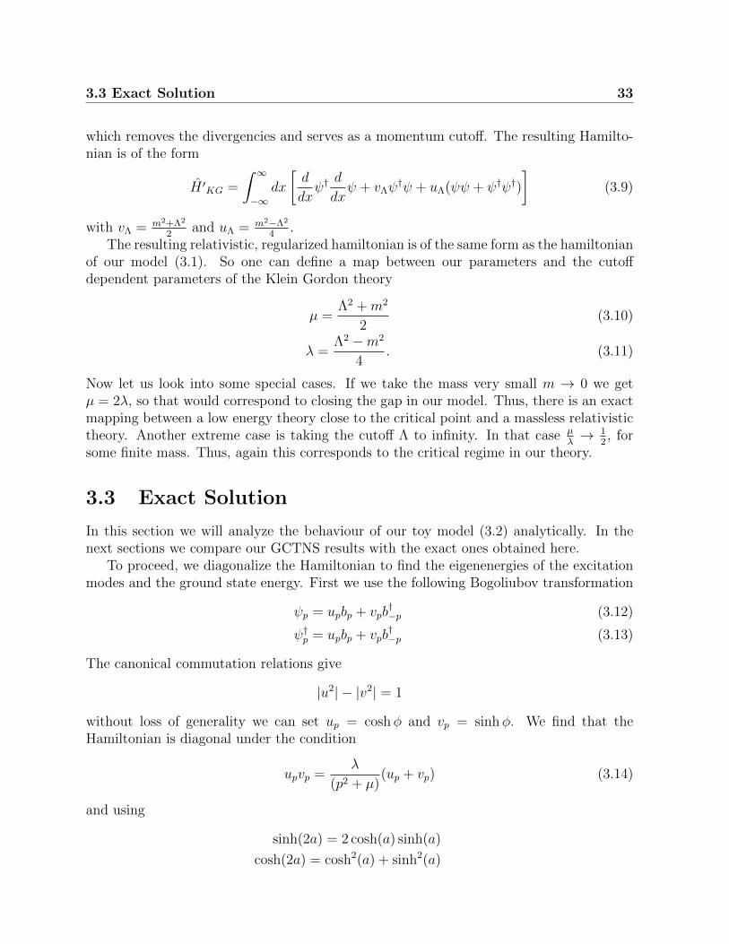
which is depicted in Fig.3.1. ∆E = ε(0) =√µ2 − 4λ2 corresponds to the gap between the
ground state and the first excited state. Our theory is well defined only for 4λ2 < µ2. Onecan see that in the limit where 4λ2 → µ2 the excitation gap is closing. Then our systemis close to the critical point and exhibits a critical behaviour. By design, with a GCTNS,we can approximate a ground state of a gapped Hamiltonian, so we will choose our modelparameters such that we are far from that point. However, we will see that even close tothe critical point we can capture some features of the states.
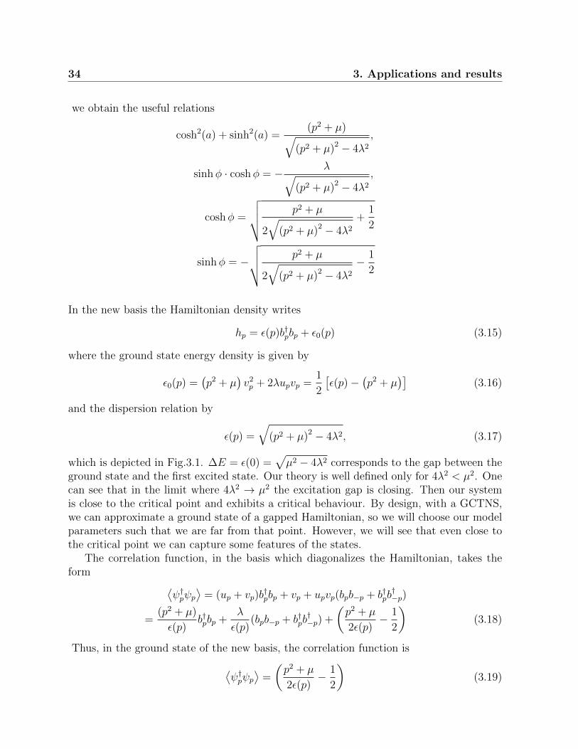
The correlation function, in the basis which diagonalizes the Hamiltonian, takes theform ⟨
ψ†pψp⟩
= (up + vp)b†pbp + vp + upvp(bpb−p + b†pb
†−p)
=(p2 + µ)
ε(p)b†pbp +
λ
ε(p)(bpb−p + b†pb
†−p) +
(p2 + µ
2ε(p)− 1
2
)(3.18)
Thus, in the ground state of the new basis, the correlation function is⟨ψ†pψp
⟩=
(p2 + µ
2ε(p)− 1
2
)(3.19)
3.3 Exact Solution 35
-1.0 -0.5 0.5 1.0
0.5
1.0
1.5
2.0
Figure 3.1: Dispersion relation of eq. (3.17) for µ = 1 and λ = 0.25 (orange),λ = 0.40(green) and at the critical point λcrit = 0.50 (blue). We can see that at the critical pointthe gap closes.
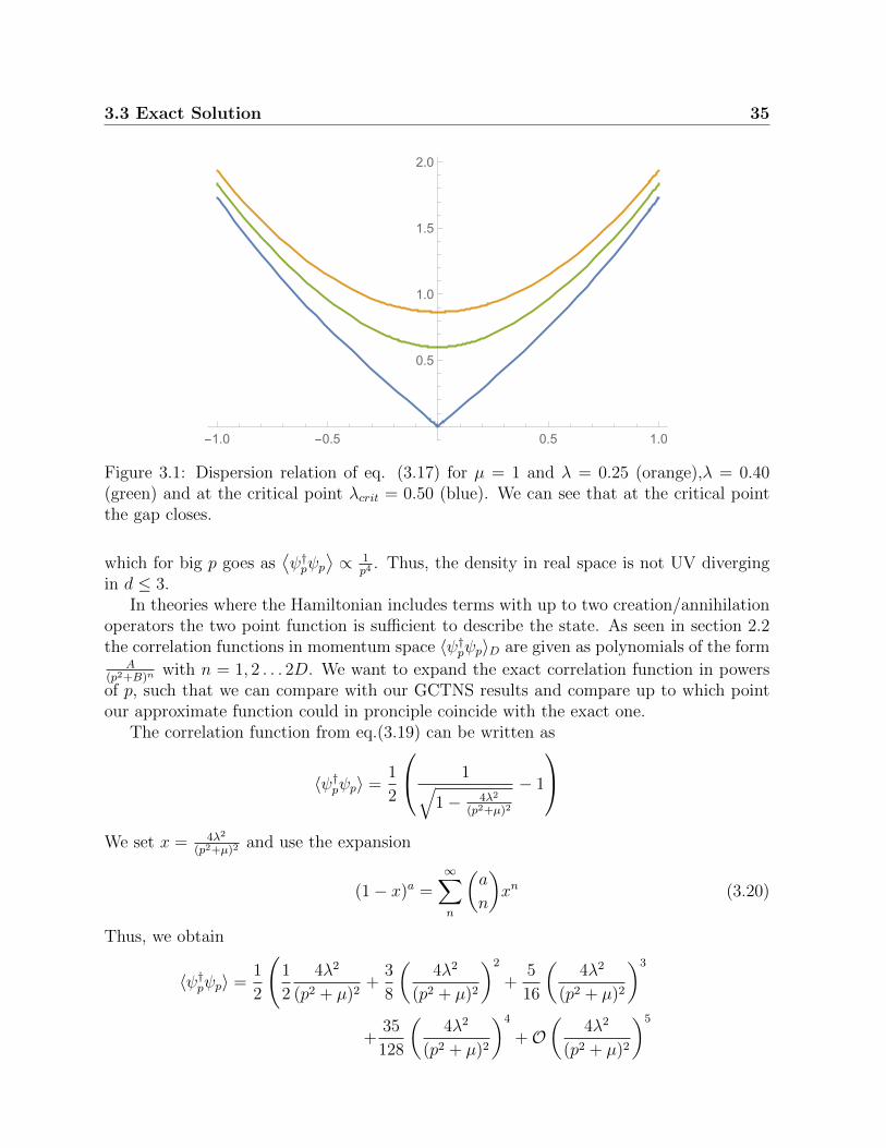
which for big p goes as⟨ψ†pψp
⟩∝ 1
p4 . Thus, the density in real space is not UV divergingin d ≤ 3.
In theories where the Hamiltonian includes terms with up to two creation/annihilationoperators the two point function is sufficient to describe the state. As seen in section 2.2the correlation functions in momentum space 〈ψ†pψp〉D are given as polynomials of the form
A(p2+B)n
with n = 1, 2 . . . 2D. We want to expand the exact correlation function in powersof p, such that we can compare with our GCTNS results and compare up to which pointour approximate function could in pronciple coincide with the exact one.
The correlation function from eq.(3.19) can be written as
〈ψ†pψp〉 =1
2
1√1− 4λ2
(p2+µ)2
− 1
We set x = 4λ2
(p2+µ)2 and use the expansion
(1− x)a =∞∑n
(a
n
)xn (3.20)
Thus, we obtain
〈ψ†pψp〉 =1
2
(1
2
4λ2
(p2 + µ)2+
3
8
(4λ2
(p2 + µ)2
)2
+5
16
(4λ2
(p2 + µ)2
)3
+35
128
(4λ2
(p2 + µ)2
)4
+O(
4λ2
(p2 + µ)2
)5
36 3. Applications and results
0 2 4 6 8 10p
0.00
0.01
0.02
0.03
0.04
0.05
0.06
0.07
0.08Exact
Corr
ela
tion f
unct
ion
Figure 3.2: The correlation function in momentum space⟨ψ†pψp
⟩for µ = 1 and λ = 0.25.
to
(3.22)
The series converges for 4λ2
(p2+µ)2 ≤ 1, thus in the non-critical regime. The series is notconverging anymore when the energy gap closes, so at the critical point.
Far from the critical point, for 4λ2 (p2 + µ)2, the leading term of the correlationfunction is
〈ψ†pψp〉 =λ2
(p2 + µ)2.
The bigger λ gets, the smaller the energy gap, the more terms in the expansion becomerelevant. Only these terms will contribute to the numerical result, so only they will beapproximated.
3.4 GCTNS in 1d
Now that we understand the model and its exact analytic solution we will use the GCTNSmethod to solve the problem variationally. As the Hamiltonian is quadratic in the creationand annihilation operators, the correlation function describes the system as well as theenergy does. Thus, we could approximate either of those quantities by our variational state.

3.4 GCTNS in 1d 37
In this report we did everything by optimizing w.r.t the energy, as for later generalizationsto different hamiltonians it is more helpful.
The first step in order to apply the variational method is to express the energy densityas the expectation value of our given Hamiltonian density
E = 〈V, a|h(x)|V, a〉 = 〈∂ψ†(x)
∂x
∂ψ(x)
∂x〉+ µ〈ψ†(x)ψ(x)〉+ λ
(〈ψ†(x)ψ†(x)〉+ 〈ψ(x)ψ(x)〉
)(3.23)
where we can compute the summands with the tools we developed in 2.2. We can startfrom some general Gaussian state
|V, a〉 =
∫Dφ exp
∫ddx(−1
2)φ(x)(−∇2 + V )φ(x) + aφ(x)ψ†(x)
|0〉,
with some initial energy Einit > E0. One can show that we can always transform theφ(x) vector by a unitary transformation, such that V is diagonal. Starting with somegeneric diagonal, complex V matrix and some complex a vector one can iteratively changethis parameters in the variational method algorithm, given by eq.(2.2) and evolve towardsstates with lower energy. The ingredients to compute the descent are given in sections2.3.1 and 2.3.2.
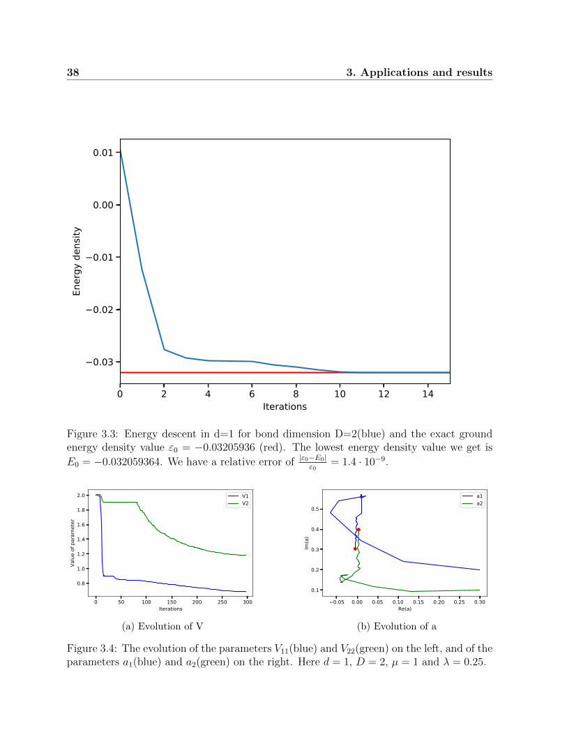
Now we perform a brief check of how well our GCTNS method works. We choose µ = 1and λ = 0.25. In this regime we are far from the critical point. In Fig. 3.3 the evolution ofthe energy density and in Fig. 3.4 and the evolution of the parameters is shown. It is donefor the simple case where D = 2 and we get E0 = −0.03205936. To benchmark our resultwe compute the lowest energy value exactly. Having the energy density in momentumspace (3.16) one can compute the energy density in real space for a translational invariantsystem
ε0 =1
L
+∞∑−∞
ε0(p) =1
π
∫ +∞
0
ε0(p)dp. (3.24)
The integral is convergent and for µ = 1 and λ = 0.25 we get ε0 = −0.03205936. Alreadyfor such a low bond dimension we see that the results of the GCTNS are very good, wehave a relative error of |ε0−E0|
ε0= 1.4 · 10−9. For higher bond dimension one expects the
results to improve. However, here the precision is already very good in D = 2.
Now we apply the same method to the case where µ = 1 and λ = 0.49 so we are closeto the critical point, which means that the energy gap from eq.(3.17) is about to close, i.e.∆E → 0. The algorithm is still stable. We expect the approximation to be worse, thanfar away from the critical point, see sections 1.1.2 and 3.4.1. The analytical value of theground state energy density now is ε0 = −0.1406884304, whereas the value we get with theGCTNS method for D=2 is E0 = −0.1406846799. Now the relative error is clearly bigger,namely |ε0−E0|
ε0= 5.3 · 10−4. It is necessary to go to higher bond dimensions in order to
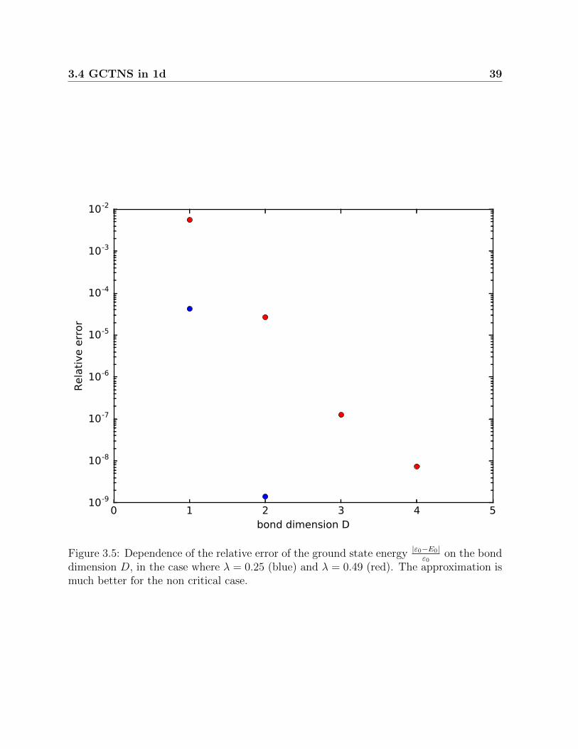
achieve higher precision. In Fig. 3.5 one can see that as we increase the bond dimensionthe actual lowest energy value is approximated better.
38 3. Applications and results
0 2 4 6 8 10 12 14Iterations
0.03
0.02
0.01
0.00
0.01
Ener
gy d
ensit
y
Figure 3.3: Energy descent in d=1 for bond dimension D=2(blue) and the exact groundenergy density value ε0 = −0.03205936 (red). The lowest energy density value we get is
E0 = −0.032059364. We have a relative error of |ε0−E0|ε0
= 1.4 · 10−9.
0 50 100 150 200 250 300Iterations
0.8
1.0
1.2
1.4
1.6
1.8
2.0
Valu
e of
par
amet
er
V1V2
(a) Evolution of V
0.05 0.00 0.05 0.10 0.15 0.20 0.25 0.30Re(a)
0.1
0.2
0.3
0.4
0.5
Im(a
)
a1a2
(b) Evolution of a
Figure 3.4: The evolution of the parameters V11(blue) and V22(green) on the left, and of theparameters a1(blue) and a2(green) on the right. Here d = 1, D = 2, µ = 1 and λ = 0.25.
3.4 GCTNS in 1d 39
0 1 2 3 4 5bond dimension D
10-9
10-8
10-7
10-6
10-5
10-4
10-3
10-2
Rela
tive e
rror
Figure 3.5: Dependence of the relative error of the ground state energy |ε0−E0|ε0
on the bonddimension D, in the case where λ = 0.25 (blue) and λ = 0.49 (red). The approximation ismuch better for the non critical case.
40 3. Applications and results
0.0 0.2 0.4 0.6 0.8 1.0p
0.01
0.02
0.03
0.04
0.05
0.06
0.07
0.08C
orr
ela
tion f
unct
ion
(a) For λ = 0.25 and µ = 1
0.00 0.02 0.04 0.06 0.08 0.10p
0.0
0.5
1.0
1.5
2.0
2.5
Corr
ela
tion f
unct
ion
(b) For λ = 0.49 and µ = 1.
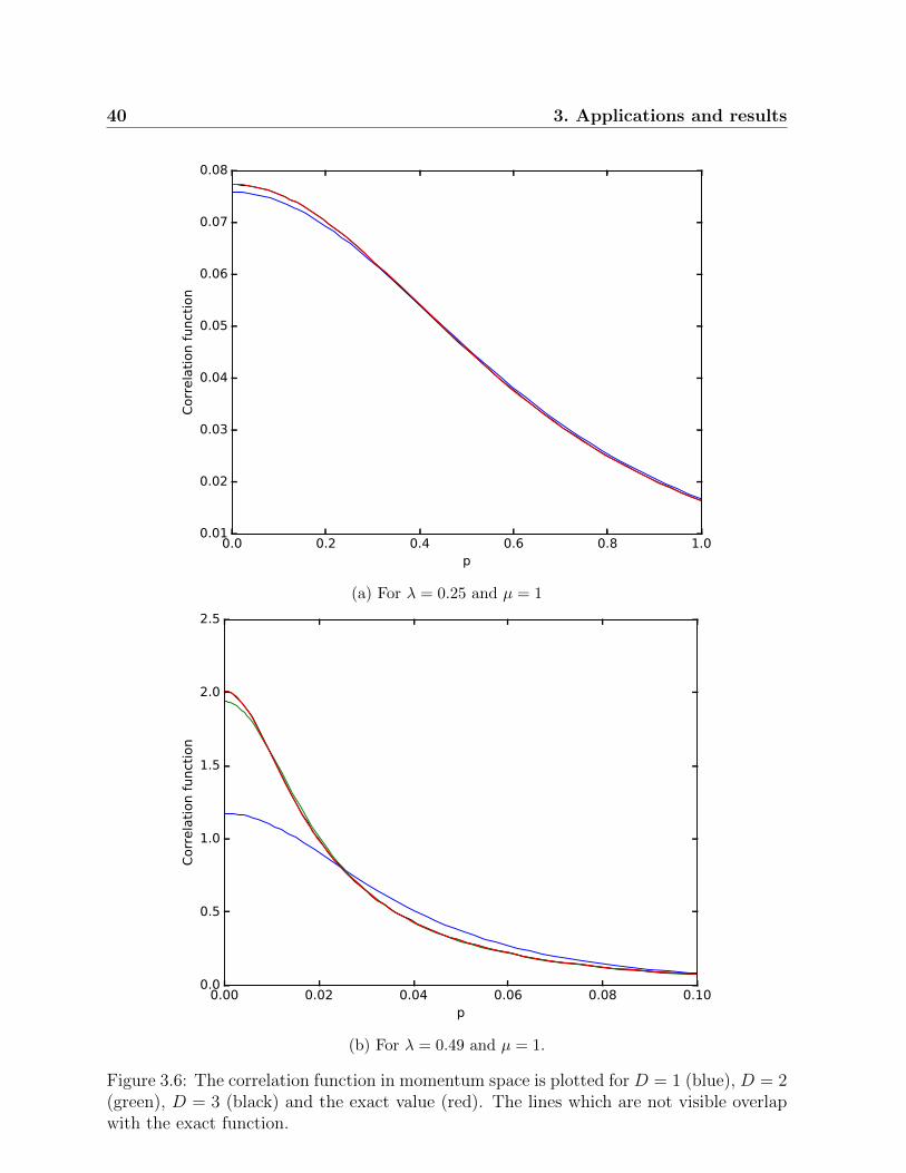
Figure 3.6: The correlation function in momentum space is plotted for D = 1 (blue), D = 2(green), D = 3 (black) and the exact value (red). The lines which are not visible overlapwith the exact function.

3.4 GCTNS in 1d 41
0 1 2 3 4bond dimension D
10-9
10-8
10-7
10-6
10-5
10-4
10-3
10-2
10-1
Dis
tance
Figure 3.7: Here the relative distance
√∫dp|〈ψ†pψp〉D=2−〈ψ†pψp〉|2∫
dp|〈ψ†pψp〉|2between the exact and the
variational correlation function 〈ψ†pψp〉D=2 is plotted, as a function of the bond dimension.Far from the critical point with µ = 1 and λ = 0.25 (blue) and close to it with µ = 1 andλ = 0.49 (red). The approximation is much better far away from the critical point.

42 3. Applications and results
3.4.1 Comparison of correlation functions
In our model a two point correlation function is also sufficient to describe a state. Eventhough we approximate with respect to the energy, we will see that the correlation func-tion also gets approximated simultaneously. The reason is that these two methods, fora quadratic Hamiltonian, are equivalent. In this subsection we will see how the GCTNScorrelation function is approximating the exact one and gain some intuition.
Lets suppose we run the program for D = 1, the simplest case. We can compute theexact form of the correlation functions
〈ψ†pψp〉D=1 =|a|4
|p2 + V |2 − |a|4(3.25)
where V and a are now simply numbers. The analytic correlation function is given by(3.21). If we take µ and λ such that we are not at the critical point, we know that thecorrelation function is very well approximated by the first terms of the expansion,
〈ψ†pψp〉 =λ2
(p2 + µ)2+ 3
(λ2
(p2 + µ)2
)2
+O
(λ2
(p2 + µ)2
2). (3.26)
The program optimizes V and a, such that the energy is minimal. This is equivallent topushing the algorithm to minimize the numerical difference between (3.25) and (3.26).
For example, after running the program for λ = 0.1 and µ = 1 we arrive at |a|2 =0.0998 ' λ and |V | = 0.98 ' µ, thus
|a|4
|p2 + V |2 − |a|4' λ2
(p2 + µ)2
As λ gets larger the second term of the expansion starts getting more important. Nowthe program still tries to fix the parameters such that it compensates for the additionalcontribution. The approximation is worse, as the 〈ψ†pψp〉D=1 function lacks terms with ap−4 dependence. If we would go to higher bond dimensions, D = 2 we would have thisdependence, so we could again find the exact solution, where (3.26) coincides with the〈ψ†pψp〉D=2. In Fig.3.6b it becomes clear that for µ = 1 and λ = 0.25 choosing D = 2 isalready sufficient. The closer we get to the critical point the more terms of the correlationexpansion become relevant and the higher we have to go in D.
The smaller the bond dimension the less parameters the program needs to optimize,but we loose in precision. The fact that the variational method is that efficient alreadyin so low bond dimensions makes it a very promising tool, as it has one main advantage,compared to the analytic solution: It could be used in principle also for non integrablemodels.
3.5 GCTNS in 2 dimensions
When implementing exactly the same gradient descent method to GCTNS in 2 spacialdimensions one encounters one main problem. The energy descent never converges, in

3.5 GCTNS in 2 dimensions 43
contrast to what we had seen in the 1 dimensional case in Fig. 3.3. The energy keeps ondecreasing and with it the values of the parameters keep on alternating. To understandthis behaviour we look at the exact analytic results. The energy density in real space
ε0 =1
4π2
∫ +∞
−∞
1
2
(√(p2 + µ)2 − 4λ2 − (p2 + µ)
)d2p
is diverging to −∞. Looking at the expansion of the integrand
ε0(p) = − λ2
(p2 + µ)− λ4
(p2 + µ)3+O
((4λ2
(p2 + µ)2
)5).
we see that integrating over p in d = 2 the first term is diverging logarithmically. Notethat in one dimension this was not the case.
Thus, the program is trying to approximate a state of infinite negative energy. Thisdoes not mean necessarily that there is no ground state, but it definately means that wecannot compare our GCTNS results with the analytic ones and that the programm willnever stop running.
We could change the algorithm and optimize the parameters with respect to the corre-lation function. In the case of a quadratic Hamiltonian, the two point function contains allthe relevant physical information of the state. Thus, approximating the two point functionis the same as approximating the lowest energy. For more generic Hamiltonian with higherorder terms, the two point function is not enough to describe the state, we also need higherorder moments. Thus, in the more generic case one is forced to proceed by minimizingthe energy. In order to have a more generic tool, we will still optimize with respect to theenergy density. Therefore we need to find a way to circumvent the problem differently.
To proceed we need to gain some more insight in the form of divergencies of the GCTNSenergy E0.
3.5.1 Divergent terms of the GCTNS
When we compute the energy for the GCTNS
E = 〈V, a|h(x)|V, a〉 = 〈∂ψ†(x)
∂x
∂ψ(x)
∂x〉+ µ〈ψ†(x)ψ(x)〉+ λ
(〈ψ†(x)ψ†(x)〉+ 〈ψ(x)ψ(x)〉
)(3.27)
we realize that some of the terms diverge in 2 dimensions, other than in 1 dimension. Forexample the closed formula for the last term is computed in 2.2
〈ψ†(x)ψ†(x)〉 =2D∑i
(a∗T · U)i(U−1 · a∗)i
∫ Λ
0
ddp
(2π)d1
p2 + λi(3.28)
=1
4π
2D∑i
(a∗T · U)i(U−1 · a∗)i[log(Λ2 + λi)−
1
4πlog(λi)] (3.29)
44 3. Applications and results
where we introduced a cutoff, as the integral∫∞
0ddp
(2π)d1
p2+λiis diverging. Similarly, the
terms 〈ψ†(x)ψ†(x)〉 and ∂2〈ψ†(x)ψ(x)〉 also contain divergent parts. We now investigatethis divergent terms and quantify their divergence.
∂2〈ψ†(x)ψ(x)〉 = log Λ2[a21 + a2
2 + ...+ a2D][a∗21 + a∗22 + ...+ a∗2D ] + finite
= log Λ2
D∑i=1
((Re[ai])
2 − (Im[ai])2)2
+ (2Re[ai]Im[ai])2 + finite (3.30)
and
〈ψ†(x)ψ†(x)〉+ 〈ψ(x)ψ(x)〉 = 2 log Λ2
D∑i=1
(Re[ai])2 − (Im[ai])
2 + finite . (3.31)
Thus, the divergent part of the energy is
f∞(a) = log Λ2
D∑i=1
((Re[ai])
2 − (Im[ai])2)2
+ (2Re[ai]Im[ai])2
+2λ[(Re[ai])
2 − (Im[ai])2]
(3.32)
We want to find the condition under which the divergent part is maximal, as it wouldcorrespond to the lowest energy. Imposing f(a)
∂Re[a1]= 0 and f(a)
∂Im[a1]= 0 we arrive at the
conditionsD∑i=1
ReaiImai = 0 (3.33)
andD∑i=1
(Re[ai])2 − (Im[ai])
2 = −λ (3.34)
So two of the parameters are dependent. These constraints keep the state ina manifold A where the energy is diverging maximally.
To get a better insight of what exactly is happening in this submanifold of states weinvestigate in the case of bond dimension D = 1. The constraints take the simple form
Rea · Ima = 0 (3.35)
(Re[a])2 − (Im[a])2 = −λ (3.36)
soa2 = −λ, (3.37)
with a ∈ R or a ∈ I .The exact form of the correlation function in that case is
〈ψ†pψp〉D=1 =|a|4
|p2 + V |2 − |a|4→ λ2
|p2 + V |2 − λ2(3.38)

3.5 GCTNS in 2 dimensions 45
H
cTNSgTNS MM
A
Figure 3.8: A ∈MGCTNS ∈McTNS ∈ H.
We see that it is very close to the form of the exact correlation function λ2
(p2+m)2 . Thus,being in that manifold allows us to still approximate the state well enough, for V ' µ.Now only one parameter is free.
On the other hand one can look at the form of the energy
E0(p) = ∂2〈ψ†pψp〉+ µ〈ψ†pψp〉+ λ(〈ψ†pψ
†−p〉+ 〈ψpψ−p〉
)= − λ2
|p2 + V |2 − λ2(p2 + µ) +
λ2(2µ− V + V ∗)
|p2 + V |2 − λ2(3.39)
As we realized in the case of the correlation function the program will optimize aroundV ' µ such that
E0(p) ' − λ2
(p2 + µ)(3.40)
which corresponds to the first term of the energy expansion, eq. (3.16).In higher D again the constraints will fix the state at a point were the energy will
diverge logarithmically. At this point, it is important to notice, that the variational classof GCTNS seems to be so good, that it can even capture the divergence of the actualground state.
3.5.2 Variational Method on non-divergent terms
It is obvious that to find the lowest energy one has to first maximize the term with thebiggest (negative) contribution. That is why we chose parameters which maximize thediverging part of the tensor network energy. Being in this submanifold of states we ensure

46 3. Applications and results
that the diverging term is maximal. We found the elements of the submanifold analytically,though one could also use numerical techniques. After being in the correct manifold weapply the same techniques as we did in 1 dimension, namely we optimize the parameterswith a variational method.
The energy can be splitted in the finite and the infinite part
E = ER + E∞ (3.41)
So when computing ER with the GCTNS method, we keep only the finite parts of the
relations 〈∂ψ†(x)∂x
∂ψ(x)∂x〉, 〈ψ†(x)ψ(x)〉, 〈ψ†(x)ψ†(x)〉 and 〈ψ(x)ψ(x)〉. Again we optimize the
paramteres such that we get the mimimal ER0 .
We can actually compare this with the finite part of the exact energy. We define εR(p)nondiverging/renormalized part of the energy as
εR0 (p) = ε0(p) +λ2
(p2 + µ)(3.42)
which we can integrate and get an exact value. For example for µ = 1 and λ = 0.25 weget
εR0 =
∫d2p
(2π)2εR0 = −0.00016630736 (3.43)
The program tries to approximate this εR0 energy. It optimizes the parameters in thesubmanifold such that ER is minimal. We get ER
0 = −0.00016565273 with a relative error
ofER
0 −εR0εR0
= 0.0039. It can be improved if we take higher bond dimensions, in analogy with
the 1 dimensional case.When looking at the resulting correlation function, Fig.3.9 and comparing it to the exact
correlation function from eq. (3.19), one can see that our tensor network approximationis very good already for D = 2. The differernce between the exact and approximate two
point function is
√∫d2p|〈ψ†pψp〉D=2−〈ψ†pψp〉|2∫
d2p|〈ψ†pψp〉|2= 1.286128 · 10−6.

3.5 GCTNS in 2 dimensions 47
0.0 0.2 0.4 0.6 0.8 1.0p
0.01
0.02
0.03
0.04
0.05
0.06
0.07
0.08
Corr
ela
tion f
unct
ion
Figure 3.9: In this graph the correlation function in momentum space is plotted. Thefunction we get with the final parameters with GCTNS (green) and the theoretical function(red) overlap, such that they are almost indistinguishable.

48 3. Applications and results

Discussion
In this report we tested the variational class of GCTNS on a simple, quasifree model, in oneand two dimensions. The results were very satisfying as the approximated ground state wasaccurate and close to the exact ground state. We were able to see the exponential decay ofthe correlation functions and approximate these sufficienlty well. Moreover, the GCTNSexpectation values inherit exactly the same infinities as the QFT. Thus, they are a goodvariational Ansatz for ground states of gaussian Hamiltonians in one and two dimensions.
The variational class we used has some main advantages compared to other Ansatze inQFTs. First, it goes beyond the classical solution, in contrast to a simple coherent state.One main property is that the number of parameters is independent of the system size.This makes it a very promising Ansatz for numerical simulations. Moreover, it is definedin arbitrary dimensions, in contrast to the one dimensional cMPS Ansatz. Its efficiencythough has not yet been tested in d > 2.
To obtain the GCTNS we kept only a very simple form of V [ψ(x)] and a[ψ(x)], see eq.(1.35). One simple generalization is to take a(0) 6= 0, which would lead to gaussian stateswith 〈ψ0〉 6= 0, thus breaking the U(1) symmetry of the ground state.
Although we have shown the efficiency of this class of states in a simple model, one couldtry out different Hamliltonians, which may be non-integrable, such as the Hamiltonian ofeq. (3.4), with quartic interactions. In that case the exact ground state is not Gaussiananymore, but still we could find the lowest energy Gaussian approximation. By takingdifferent functions of V [ψ(x)] and a[ψ(x)], with higher order terms, one could create acTNS which goes beyond Gaussian states. However, computing expectation values in thatcase is impossible, because of the form of the generating functional (1.30). Therefore onehas to keep the GCTNS Ansatz, but could add some perturbation.
The QTNS could also provide a natural continuum version of tensor network toy modelsof the AdS/CFT correspondence, where scalar field theories on a fixed AdS background arerelated to conformal field theories on the boundary. One could realize such conditions withGCTNS with the physical field ψ living on the boundary of a two dimensional auxiliaryspace, populated by the fields φ.
Moreover, many interesting questions are so far open. How do V and a encode topo-logical order? Do cTNS generically obey the area law like their discrete counterparts? Towhat extent does the bond field dimension D quantify entanglement for classes of cTNS?Tackling these questions is an important goal for future work, to fully extend the successof tensor networks from the lattice to the continuum.

50 3. Applications and results

Appendices


Appendix A
Appendix: Tensor Network Notation
This is a small overview over the Tensor Network notation and the main Tensor operations.For further understanding, one can read the following literature [5, 1]. Tensors are thegeneralization of vectors and matrices. A d- dimensional vector can be considered as anelement of Cd, and an n × m dimensional matrix an element of Cn×m. Correspondinglyan rank-r tensor of dimensions d1 × d2 × ... × dr is an element of Cd1×d2×...×dr . In tensornetwork notation a single tensor will be represented by a geometric shape with legs stickingout of it, each corresponding to one index, like in these examples of a vector, a matrix anda 3-rank tensor respectively:
k
lm n
TTklmn=vj= j Amn= A nmv
The first operation we will consider is the tensor product, a generalization of the outerproduct of vectors. The tensor product of A ∈ Cd1×d2×...×dr and B ∈ Cd1×d2×...×dn is
[A⊗B]i1,i2...ir,j1,j2,...js = Ai1,i2...ir ·Bj1,j2,...js ∈ (Cd1×...×dr ⊗ Cd1×...×dn) (A.1)
and is represented as
A Bx=A B
Given a tensor A, for which the xth and yth indices have identical dimensions (dx = dy),the partial trace over these two dimensions is simply a joint summation over that index
[Trx,yA]i1,i2...ix−1,ix+1,..,iy−1,iy+1...ir =dx∑a
Ai1,i2...ix−1,a,ix+1,..,iy−1,a,iy+1...ir , (A.2)
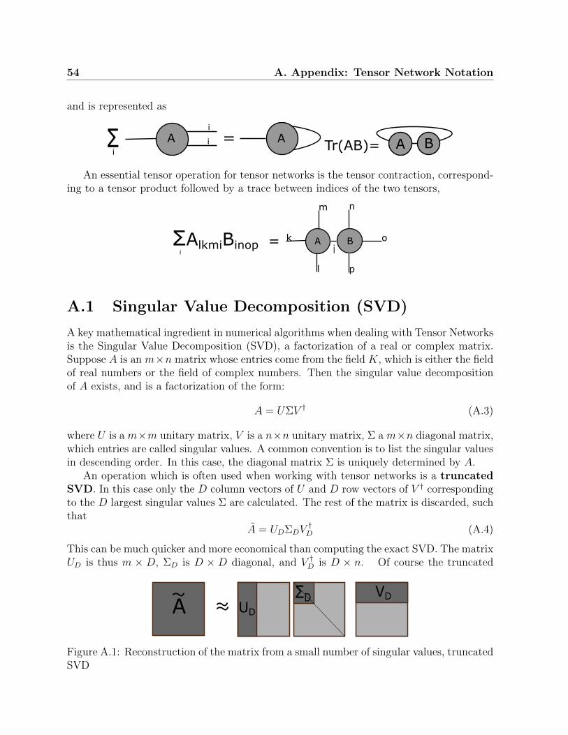
54 A. Appendix: Tensor Network Notation
and is represented as
=Σi
i
iA A Tr(AB)= A B
An essential tensor operation for tensor networks is the tensor contraction, correspond-ing to a tensor product followed by a trace between indices of the two tensors,
BAk
l
m n
o
p
iΣiAlkmiBinop =
A.1 Singular Value Decomposition (SVD)
A key mathematical ingredient in numerical algorithms when dealing with Tensor Networksis the Singular Value Decomposition (SVD), a factorization of a real or complex matrix.Suppose A is an m×n matrix whose entries come from the field K, which is either the fieldof real numbers or the field of complex numbers. Then the singular value decompositionof A exists, and is a factorization of the form:
A = UΣV † (A.3)
where U is a m×m unitary matrix, V is a n×n unitary matrix, Σ a m×n diagonal matrix,which entries are called singular values. A common convention is to list the singular valuesin descending order. In this case, the diagonal matrix Σ is uniquely determined by A.
An operation which is often used when working with tensor networks is a truncatedSVD. In this case only the D column vectors of U and D row vectors of V † correspondingto the D largest singular values Σ are calculated. The rest of the matrix is discarded, suchthat
A = UDΣDV†D (A.4)
This can be much quicker and more economical than computing the exact SVD. The matrixUD is thus m × D, ΣD is D × D diagonal, and V †D is D × n. Of course the truncated
A UDΣD VD
Figure A.1: Reconstruction of the matrix from a small number of singular values, truncatedSVD

A.2 Tensor Networks 55
SVD is no longer an exact decomposition of the original matrix A, but the approximatematrix A is in a very useful sense the closest approximation to A that can be achieved bya matrix of rank D.
A.2 Tensor Networks
A Tensor Network is a diagram which tells us how to combine several tensors into a singlecomposite tensor. The rank of this overall tensor is given by the number of unmatchedtensor legs. Tensor networks can be contracted by beginning with a single tensor and
A A AA A A
(a) A zero rank tensor, just a number.
A A AA A A
i1 i2 i3 i4 i5 i6
(b) 6 rank tensor
Figure A.2: Examples of 1 dimensional Tensor networks. From the diagram one can readhow to contract the matrices(a) or tensors(b).
repeatedly contracting it against tensors one at a time. For example the composite tensorof Fig.A.3b can be computed iteratively by contracting more and more tensors together,as seen in Fig. A.4. It is important to note that the form/rank of the tensors in d ≥ 2changes, while in d = 1 it stays the same. By applying this grouping iteratively we cancompute the final overall tensor.
While in the simple 1 dimensional case this is trivial, in 2 dimensions it is not. First,there are different lattice structures, as triangular lattices, tree-like and MERA structures[14]. Furthermore, one can notice that there are computationally cheaper ways to computethe final tensor. Many different methods of contracting the tensors have been developedover the years, as boundary MPS [30], corner transfer matrices [31] and Tensor coarsegraining [32]. In the latter we group neighboring tensors into new, higher rank tensors, seeFig.A.5.
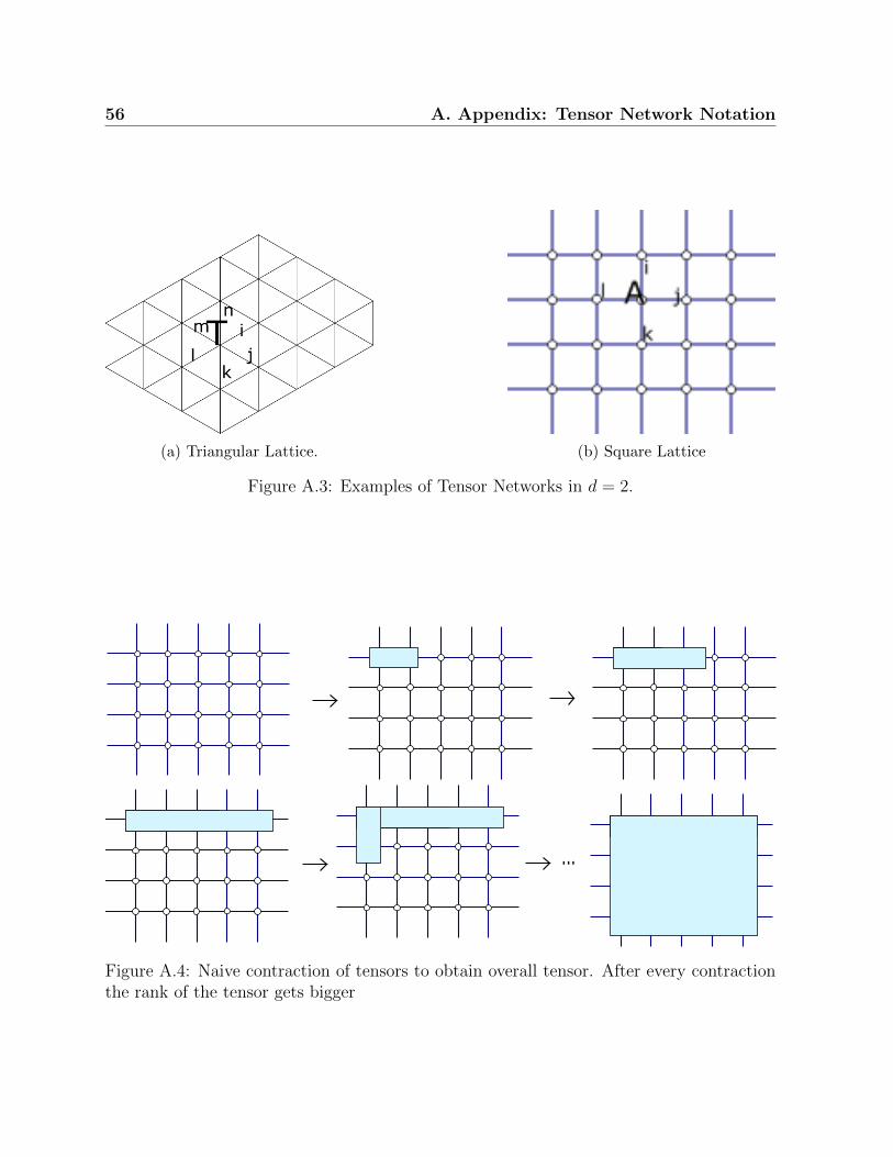
56 A. Appendix: Tensor Network Notation
(a) Triangular Lattice. (b) Square Lattice
Figure A.3: Examples of Tensor Networks in d = 2.
...
Figure A.4: Naive contraction of tensors to obtain overall tensor. After every contractionthe rank of the tensor gets bigger
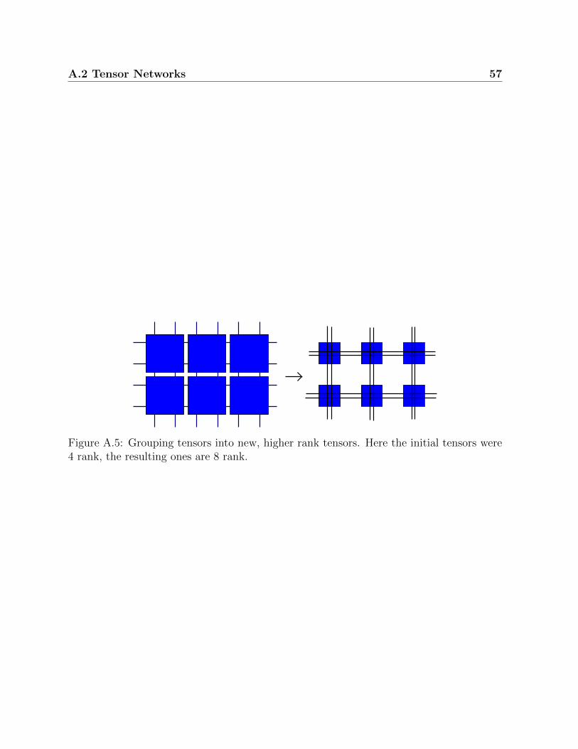
A.2 Tensor Networks 57
Figure A.5: Grouping tensors into new, higher rank tensors. Here the initial tensors were4 rank, the resulting ones are 8 rank.

58 A. Appendix: Tensor Network Notation

Appendix B
Appendix: Path integral formulation
We can reformulate the cMPS state so that expectation values for the auxiliary systemare expressed as path integrals [23]. The motivation is to expand the cMPS to higherdimensions, respecting the symmetries of the physical state in terms of symmetries ofan action for the auxiliary system. We will explain only the similarity between a tensorcontraction and a path integral over an auxiliary field in the simple case of a cMPS.
We start by writing a basis for the auxiliary Hilbert spaceHaux as |j〉aux with j = 1..., D.We enlarge the space via second quantization, and introduce bosonic annihilation andcreation operators bj and b†j with [bj, b
†i ] = δij. The Hilbert space of the enlarged auxiliary
system is that of the Fock space F(Haux), which is infinite dimensional. The connectionbetween the two spaces is made by identifying Haux with the single particle sector via|j〉aux = b†j|Ω >aux. Now we make the following substitution
Q(x)→ Qi,j(x)b†jbi, (B.1)
R(x)→ Ri,j(x)b†jbi (B.2)
and obtain the action
S(x) =∑i,j
Qi,j(x)b†jbi ⊗ 1 +Ri,j(x)b†jbi ⊗ ψ†(x) (B.3)
We divide the space [0, L] in small intervals with uniform spacing ε and insert resolutionsof the identity
1 =1
πD
∫ D∏k
dφkdφ∗k|φk〉〈φk| (B.4)
where φk = exp[φkb†k − φ∗kbk]|Ω >aux is a field coherent bosonic state. Taking the limit
where ε→ 0 and assuming that only smooth variations of the auxiliary field φ contribute,we obtain a path integral
|χ〉 =
∫DφDφ∗ exp
∫ L
0
(1
2φ†(x)
dφ
dx(x) +
dφ∗
dx(x)φ(x)
+φ†(x)Q(x)φ(x) + (φ†(x)R(x)φ(x))ψ†(x)dx|Ω〉

60 B. Appendix: Path integral formulation
to
(B.6)
where φ = φkDk=1 is a vector field. The formulation of the cMPS as a path integral isguiding expression for the generalization to higher dimensional scenarios, which will bedescribed in section 1.3.
Appendix C
Appendix: Integrals
The integrals computed here we need in order to implement the variational code, as wewill need to arrive at closed formulas. We only need integrals over momenta in one andtwo spacial dimensions, as we restrict only to these cases in our example models.
C.1 One dimension
We compute the same integrals in 1 dimension
I1(λi) =
∫dp
2π
1
p2 + λieip(x−y) =
1
2√λi
I1kin(λi) =
∫dp
2π
p2
p2 + λieip(x−y)
= −√λi2
(C.1)
I2(λi, λj) = limx→y
∫ddp
(2π)d1
p2 + λi
1
p2 + λjeip(x−y) (C.2)
for x→ y we get
I2(λi 6= λj) = − 1
2(√λi +
√λj)(√λi√λj)
(C.3)
I2(λi = λj) =1
4√λi
3 (C.4)
I2kin(λi, λj) = limx→y
∫d2p
(2π)dp2
p2 + λi
1
p2 + λjeip(x−y) (C.5)

62 C. Appendix: Integrals
for x→ y we get
I2kin(λi 6= λj) =1
2(√λi +
√λj)
(C.6)
I2kin(λi = λj) =1
4√λi
(C.7)
for Λ λi
I2kin(λi 6= λj) =1
2πln Λ− 1
4π
λi ln (λi)− λj ln (λj)
λi − λj(C.8)
I2kin(λi = λj) =1
4π[2 log(Λ)− 1− log(λi)] (C.9)
C.2 Two dimensions
We will compute integrals of the form In =∫
d2p(2π)2Cn(p)eip(x−y). We are interested in
the case where x → y, because we use only equal point correlation functions. In ourcomputations we insert a cutoff Λ whenever the integral is divergent, to quantify thedivergence. In order to obtain the initial integral one has to take Λ→∞.
I1(λi) =
∫d2p
(2π)2
1
p2 + λieip(x−y)
=
∫ Λ2
0
d(p2)
4π
1
p2 + λi
=1
4πlog(Λ2 + λi)−
1
4πlog(λi) (C.10)
I1kin(λi) =
∫d2p
(2π)2
p2
p2 + λieip(x−y)
=
∫ Λ2
0
dp2
4π
p2
p2 + λi
=1
4π[Λ2 − λiln(Λ2 + λi) + λiln(λi)] (C.11)
I2(λi, λj) = limx→y
∫ddp
(2π)d1
p2 + λi
1
p2 + λjeip(x−y) (C.12)
C.2 Two dimensions 63
for x→ y we get
I2(λi 6= λj) =
∫ ∞0
dp
2π
p
(p2 + λi)(p2 + λj)
=1
4π
∫ ∞0
dp2
(p2 + λi)(p2 + λj)
=1
4π
∫ ∞λi
du1
u · (u− λi + λj), u = p2 + λi
=1
4π(λi − λj)
∫ ∞λi
du[1
u− 1
u− λi + λj]
=ln(λi/λj)
4π(λi − λj)(C.13)
I2(λi = λj) =1
4π
∫ ∞λi
d(p2 + λi)
(p2 + λi)2
=1
4πλi(C.14)
I2kin(λi, λj) = limx→y
∫d2p
(2π)dp2
p2 + λi
1
p2 + λjeip(x−y) (C.15)
for x→ y we get
I2kin(λi 6= λj) =
∫d2p
(2π)2
p2
p2 + λi
1
p2 + λj
=
∫ Λ2
0
dp2
4π
p2
p2 + λi
1
p2 + λj
=1
4π
λi ln (λi + Λ2)− λj ln (λj + Λ2)
λi − λj− 1
4π
λi ln (λi)− λj ln (λj)
λi − λj(C.16)
I2kin(λi = λj) =1
4π
[λi
λi + Λ2+ log(Λ2 + λi)− 1− log(λi)
](C.17)
for Λ λi
I2kin(λi 6= λj) =1
2πln Λ− 1
4π
λi ln (λi)− λj ln (λj)
λi − λj(C.18)
I2kin(λi = λj) =1
4π[2 log(Λ)− 1− log(λi)] (C.19)
I3(V, a, κi, κj, λn) =
∫ Λ
0
d2p
(2π)2
1
p2 + κi
1
p2 + κj
1
p2 + λn(C.20)
64 C. Appendix: Integrals
For κi 6= κj and Λ λn
I3(V, a, κi, κj, λn) = − 1
4π
(κj − λn) lnκi + (λn − κi) lnκj + (κi − κj) lnλn(κj − λn)(κi − λn)(κi − κj)
, (C.21)
and for κi = κj and Λ λn
I3(V, a, κi = κj, λn) = − 1
4π
κi lnλn − κi lnκi + κi − λnκi(κi − λn)2
(C.22)
and for λn = κi = κj and Λ λn
I3(V, a, κi = κj = λn) = − 1
8πκ2i
(C.23)
Bibliography
[1] Roman Orus, A Practical Introduction to Tensor Networks:Matrix Product States andProjected Entangled Pair States, Institute of Physics, Johannes Gutenberg University(2014).
[2] Roman Orus, Tensor networks for complex quantum systems, Nature Reviews Physicsvolume 1, pages 538–550 (2019).
[3] F. Verstraete, J.I. Cirac, V. Murg, Matrix product states, projected entangled pairstates, and variational renormalization group methods for quantum spin systems, Adv.Phys.57, 143(2008).
[4] J. I. Cirac and F. Verstraete, Renormalization and Tensor Product States in SpinChains and Lattices,J. Phys. A42,504004 (2009).
[5] J. C. Bridgeman and C. T. Chubb, Hand-Waving and Interpretive Dance: An Intro-ductory Course on Tensor Networks, J. Phys. A50, 223001 (2017).
[6] Time-evolution methods for matrix-product states,S. Paeckela, T. Kohler, A. Swobodac,S. R. Manmanaa, U. Schollwockc ,C. Hubig, https://arxiv.org/pdf/1901.05824.pdf
[7] Piotr Czarnik and Jacek Dziarmaga, Time evolution of an infinite projected entangledpair state: An algorithm from first principles, Phys. Rev. B 98, 045110 (2018)
[8] F. Pollmann, A. M. Turner, E. Berg, and M. Oshikawa, Entanglement Spectrum of aTopological Phase in One Dimension, Phys. Rev. B81, 064439 (2010).
[9] N. Schuch, D. Perez-Garcıa, and .I Cirac, Classifying Quantum Phases Using MatrixProduct States and Projected Entangled Pair States,Phys. Rev. B84, 165139(2011).
[10] H. A. Kramers , G. H. Wannier, Statistics of the two-dimensional ferromagnet, PartII. Phys. Rev.60, 263 (1941).
[11] S. R. White, Density matrix formulation for quantum renormalization groups. Phys.Rev. Lett.69, 28632866 (1992).

66 BIBLIOGRAPHY
[12] U. Schollwock, The density Matrix Renormalization Group, Rev. Mod. Phys. 77, 259(2005)
[13] F. Verstraete, J. I. Cirac, Renormalization algorithms for quantum- many bodysystems in two and higher dimensions. Preprint at https://arxiv.org/abs/cond-mat/0407066 (2004).
[14] G. Vidal, Entanglement renormalization, Phys. Rev. Lett.99, 220405 (2007).
[15] B. Swingle, Entanglement renormalization and holography, Phys. Rev. D86, 065007(2012).
[16] M. M. Wolf, F. Verstraete, M. B. Hastings, and J. I. Cirac, Area Laws in QuantumSystems: Mutual Information andCorrelations, Phys. Rev. Lett.100, 070502 (2008)
[17] M. B. Hastings, Solving gapped Hamiltonians locally. Phys. Rev. B73, 085115 (2006).
[18] F. Verstraete, J.I. Cirac, Continuous Matrix Product States for quantum Fields, Phys.Rev. Lett. 104, 190405 (2010).
[19] J. Haegeman, J. I. Cirac, T. J. Osborne, and F. Verstraete, Calculus of ContinuousMatrix Product States,Phys. Rev. B88, 085118 (2013).
[20] J. Haegeman, T. J. Osborne, H. Verschelde, F. Verstraete, Entanglement renormal-ization for quantum fields in real space, Phys. Rev. Lett.110, 100402 (2013).
[21] C. Brockt, J. Haegeman, D. Jennings, T.J. Osborne F. Verstraete, The continuumlimit of a tensor network: a path integral representation., arXiv:1210.5401
[22] Antoine Tilloy, J. Ignacio Cirac, Continuous Tensor Network States for QuantumFields, Phys.Rev.X 9,021040 (2019).
[23] D. Jennings, C. Brockt, J. Haegeman, T.J. Osborne, and F. Verstraete, Contin-uum Tensor Network Field States, Path Integral Representations and Spatial Symme-tries,New J.Phys.17, 063039 (2015).
[24] Riccardo Borghi, The variational method in quantum mechanics: An elementary in-troduction, Eur. J. Phys.39 035410 (2018)
[25] J. Haegeman, J. I. Cirac, T. J. Osborne, H. Verschelde, and F. Verstraete,Applying the Variational Principle to (11)-Dimensional Quantum Field Theories,Phys. Rev. Lett. 105,251601 (2010)
[26] G. Vidal, Efficient classical simulation of slightly entangled quantum computations.Phys. Rev. Lett.91, 147902 (2003).
[27] M.B. Hastings, An Area Law for One Dimensional Quantum Systems, J.Stat.Mech.,P08024 (2007).
BIBLIOGRAPHY 67
[28] E. H. Lieb and W. Liniger, Phys. Rev. 130, 1605 (1963)
[29] V. Stojevic, J. Haegeman, I. P. McCulloch, L. Tagliacozzo, F. Verstraete, ConformalData from Finite Entanglement Scaling, arXiv:1401.7654
[30] J. Jordan,R. Orus,G. Vidal, F. Verstraete, J. I. Cirac, Classical simulation of infinite-size quantum lattice systems in two spatial dimensions. Phys. Rev. Lett.101, 250602(2008).
[31] R. Orus, G. Vidal, Simulation of two- dimensional quantum systems on an infinitelattice revisited: corner transfer matrix for tensor contraction. Phys. Rev. B80, 094403(2009).
[32] M. Levin, C. P. Nave, Tensor renormalization group approach to two- dimensionalclassical lattice models, Phys. Rev. Lett.99, 120601 (2007)
[33] T. Guaita, L. Hackl, T. Shi, C. Hubig, E. Demler, J. Ignacio Cirac Gaussian timedependent variational principle for the Bose-Hubbard model, Phys. Rev. B 100, 094529(2019)