continuous online sequence learning with an unsupervised ...€¦ · continuous online sequence...

LETTER Communicated by Jurgen Schmidhuber

Continuous Online Sequence Learning with an UnsupervisedNeural Network Model

Yuwei [email protected] [email protected] [email protected], Inc. Redwood City, CA 94063, U.S.A.

The ability to recognize and predict temporal sequences of sensory in-puts is vital for survival in natural environments. Based on many knownproperties of cortical neurons, hierarchical temporal memory (HTM) se-quence memory recently has been proposed as a theoretical frameworkfor sequence learning in the cortex. In this letter, we analyze properties ofHTM sequence memory and apply it to sequence learning and predictionproblems with streaming data. We show the model is able to continuouslylearn a large number of variable order temporal sequences using an unsu-pervised Hebbian-like learning rule. The sparse temporal codes formedby the model can robustly handle branching temporal sequences by main-taining multiple predictions until there is sufficient disambiguating ev-idence. We compare the HTM sequence memory with other sequencelearning algorithms, including statistical methods—autoregressive inte-grated moving average; feedforward neural networks—time delay neuralnetwork and online sequential extreme learning machine; and recurrentneural networks—long short-term memory and echo-state networks onsequence prediction problems with both artificial and real-world data.The HTM model achieves comparable accuracy to other state-of-the-artalgorithms. The model also exhibits properties that are critical for se-quence learning, including continuous online learning, the ability tohandle multiple predictions and branching sequences with high-orderstatistics, robustness to sensor noise and fault tolerance, and good per-formance without task-specific hyperparameter tuning. Therefore, theHTM sequence memory not only advances our understanding of howthe brain may solve the sequence learning problem but is also applicableto real-world sequence learning problems from continuous data streams.

Neural Computation 28, 2474–2504 (2016) c© 2016 Massachusetts Institute of Technology.doi:10.1162/NECO_a_00893 Published under a Creative Commons

Attribution 3.0 Unported (CC BY 3.0) license.

Online Learning with HTM Sequence Memory 2475

1 Introduction

In natural environments, the cortex continuously processes streams of sen-sory information and builds a rich spatio temporal model of the world.The ability to recognize and predict ordered temporal sequences is criticalto almost every function of the brain, including speech recognition, activetactile perception, and natural vision. Neuroimaging studies have demon-strated that multiple cortical regions are involved in temporal sequenceprocessing (Clegg, Digirolamo, & Keele, 1998; Mauk & Buonomano, 2004).Recent neurophysiology studies have shown that even neurons in primaryvisual cortex can learn to recognize and predict spatiotemporal sequences(Gavornik & Bear, 2014; Xu, Jiang, Poo, & Dan, 2012) and that neurons inprimary visual and auditory cortex exhibit sequence sensitivity (Brosch &Schreiner, 2000; Nikolic, Hausler, Singer, & Maass, 2009). These studies sug-gest that sequence learning is an important problem that is solved by manycortical regions.

Machine learning researchers have also extensively studied sequencelearning independent of neuroscience. Statistical models, such as hiddenMarkov models (HMM; Fine, Singer, & Tishby, 1998; Rabiner & Juang,1986) and autoregressive integrated moving average (ARIMA; Durbin &Koopman, 2012), have been developed for temporal pattern recognitionand time-series prediction, respectively. A variety of neural network mod-els have been proposed to model sequential data. Feedforward networkssuch as time-delay neural networks (TDNN) have been used to model se-quential data by adding a set of delays to the input (Waibel, Hanazawa,Hinton, Shikano, & Lang, 1989). Recurrent neural networks can model se-quence structure with recurrent lateral connections and process the datasequentially one record at a time. For example, long short-term memory(LSTM) has the ability to selectively pass information across time and canmodel very long-term dependencies using gating mechanisms (Hochreiter& Schmidhuber, 1997) and gives impressive performance on a wide va-riety of real-world problems (Greff, Srivastava, Koutnik, Steunebrink, &Schmidhuber, 2015; Lipton, Berkowitz, & Elkan, 2015; Sutskever, Vinyals,& Le, 2014). Echo state network (ESN) uses a randomly connected recur-rent network as a dynamics reservoir and models a sequence as a trainablelinear combination of these response signals (Jaeger & Haas, 2004).

Can machine learning algorithms gain any insight from cortical algo-rithms? The current state-of-the-art statistical and machine learning algo-rithms achieve impressive prediction accuracy on benchmark problemsHowever, most time-series prediction benchmarks do not focus on modelperformance in dynamic, nonstationary scenarios. Benchmarks typicallyhave separate training and testing data sets, where the underlying assump-tion is that the test data share similar statistics as the training data (Ben Taieb,Bontempi, Atiya, & Sorjamaa, 2012; Crone, Hibon, & Nikolopoulos, 2011).In contrast, sequence learning in the brain has to occur continuously to deal

2476 Y. Cui, S. Ahmad, and J. Hawkins

with the noisy, constantly changing streams of sensory inputs. Notably,with the increasing availability of streaming data, there is also an increas-ing demand for online sequence algorithms that can handle complex, noisydata streams. Therefore, reverse-engineering the computational principlesused in the brain could offer additional insights into the sequence learningproblem that lies at the heart of many machine learning applications.

The exact neural mechanisms underlying sequence memory in the brainremain unknown, but biologically plausible models based on spiking neu-rons have been studied. For example, Rao and Sejnowski (2001) showedthat spike-time-dependent plasticity rules can lead to predictive sequencelearning in recurrent neocortical circuits. Spiking recurrent network mod-els have been shown to recognize and recall precisely timed sequences ofinputs using supervised learning rules (Brea, Senn, & Pfister, 2013; Ponulak& Kasinski, 2010). These studies demonstrate that certain limited types ofsequence learning can be solved with biologically plausible mechanisms.However, only a few practical sequence learning applications use spikingnetwork models as these models recognize only relatively simple and lim-ited types of sequences. These models also do not match the performanceof nonbiological statistical and machine learning approaches on real-worldproblems.

In this letter, we present a comparative study of HTM sequence mem-ory, a detailed model of sequence learning in the cortex (Hawkins & Ah-mad, 2016). The HTM neuron model incorporates many recently discoveredproperties of pyramidal cells and active dendrites (Antic, Zhou, Moore,Short, & Ikonomu, 2010; Major, Larkum, & Schiller, 2013). Complex se-quences are represented using sparse distributed temporal codes (Ahmad& Hawkins, 2016; Kanerva, 1988), and the network is trained using an on-line unsupervised Hebbian-style learning rule. The algorithms have beenapplied to many practical problems, including discrete and continuous se-quence prediction, anomaly detection (Lavin & Ahmad, 2015), and sequencerecognition and classification.

We compare HTM sequence memory with four popular statistical andmachine learning techniques: ARIMA, a statistical method for time-seriesforecasting (Durbin & Koopman 2012); extreme learning machine (ELM),a feedforward network with sequential online learning (Huang, Zhu, &Siew, 2006; Liang, Huang, Saratchandran, & Sundararajan, 2006); and tworecurrent networks, LSTM and ESN. We show that HTM sequence mem-ory achieves comparable prediction accuracy to these other techniques. Inaddition, it exhibits a set of features that is desirable for real-world se-quence learning from streaming data. We demonstrate that HTM networkslearn complex high-order sequences from data streams, rapidly adapt tochanging statistics in the data, naturally handle multiple predictions andbranching sequences, and exhibit high tolerance to system faults.

The letter is organized as follows. In section 2, we discuss a list of desiredproperties of sequence learning algorithms for real-time streaming data


analysis. In section 3, we introduce the HTM temporal memory model. Insections 4 and 5, we apply the HTM temporal memory and other sequencelearning algorithms to discrete artificial data and continuous real-worlddata, respectively. Discussion and conclusions are given in section 6.

2 Challenges of Real-Time Streaming Data Analysis

With the increasing availability of streaming data, the demand for onlinesequence learning algorithms is increasing. Here, a data stream is an or-dered sequence of data records that must be processed in real time usinglimited computing and storage capabilities. In the field of data stream min-ing, the goal is to extract knowledge from continuous data streams such ascomputer network traffic, sensor data, and financial transactions (Domin-gos & Hulten, 2000; Gaber, Zaslavsky, & Krishnaswamy, 2005; Gama, 2010),which often have changing statistics (nonstationary) (Sayed-Mouchaweh &Lughofer, 2012). Real-world sequence learning from such complex, noisydata streams requires many other properties in addition to prediction accu-racy. This stands in contrast to many machine learning algorithms, whichare developed to optimize performance on static data sets and lack theflexibility to solve real-time streaming data analysis tasks.

In contrast to these algorithms, the cortex solves the sequence learn-ing problem in a drastically different way. Rather than achieving optimalperformance for a specific problem (e.g., through gradient-based optimiza-tion), the cortex learns continuously from noisy sensory input streams andquickly adapts to the changing statistics of the data. When information is in-sufficient or ambiguous, the cortex can make multiple plausible predictionsgiven the available sensory information.

Real-time sequence learning from data streams presents unique chal-lenges for machine learning algorithms. In addition to prediction accuracy,we list a set of criteria that apply to both biological systems and real-worldstreaming applications.

2.1 Continuous Learning. Continuous data streams often have chang-ing statistics. As a result, the algorithm needs to continuously learn fromthe data streams and rapidly adapt to changes. This property is impor-tant for processing continuous real-time sensory streams but has not beenwell studied in machine learning. For real-time data stream analysis, it isvaluable if the algorithm can recognize and learn new patterns rapidly.

Machine learning algorithms can be classified into batch or online learn-ing algorithms. Both types of algorithms can be adopted for continuouslearning applications. To apply a batch-learning algorithm to continuousdata stream analysis, one needs to keep a buffered data set of past datarecords. The model is retrained at regular intervals because the statisticsof the data can change over time. The batch-training paradigm poten-tially requires significant computing and storage resources, particularly in


situations where the data velocity is high. In contrast, online sequential al-gorithms can learn sequences in a single pass and do not require a buffereddata set.

2.2 High-Order Predictions. Real-world sequences contain contextualdependencies that span multiple time steps (i.e., the ability to make high-order predictions). The term order refers to Markov order, specifically theminimum number of previous time steps the algorithm needs to considerin order to make accurate predictions. An ideal algorithm should learn theorder automatically and efficiently.

2.3 Multiple Simultaneous Predictions. For a given temporal context,there could be multiple possible future outcomes. With real-world data, itis often insufficient to consider only the single best prediction when infor-mation is ambiguous. A good sequence learning algorithm should be ableto make multiple predictions simultaneously and evaluate the likelihood ofeach prediction online. This requires the algorithm to output a distributionof possible future outcomes. This property is present in HMMs (Rabiner &Juang, 1986) and generative recurrent neural network models (Hochreiter& Schmidhuber, 1997), but not in other approaches like ARIMA, which arelimited to maximum likelihood prediction.

2.4 Noise Robustness and Fault Tolerance. Real-world sequence learn-ing deals with noisy data sources where sensor noise, data transmissionerrors, and inherent device limitations frequently result in inaccurate ormissing data. A good sequence learning algorithm should exhibit robust-ness to noise in the inputs.

The algorithm should also be able to learn properly in the event of sys-tem faults such as loss of synapses and neurons in a neural network. Theproperty of fault tolerance and robustness to failure, present in the brain,is important for the development of next-generation neuromorphic proces-sors (Tran, Yanushkevich, Lyshevski, & Shmerko, 2011). Noise robustnessand fault tolerance ensure flexibility and wide applicability of the algorithmto a wide variety of problems.

2.5 No Hyperparameter Tuning. Learning in the cortex is extremelyrobust for a wide range of problems. In contrast, most machine learningalgorithms require optimizing a set of hyperparameters for each task. Ittypically involves searching through a manually specified subset of the hy-perparameter space, guided by performance metrics on a cross-validationdata set. Hyperparameter tuning presents a major challenge for applica-tions that require a high degree of automation, like data stream mining. Anideal algorithm should have acceptable performance on a wide range ofproblems without any task-specific hyperparameter tuning.


Many of the existing machine learning techniques demonstrate theseproperties to various degrees. A truly flexible and powerful system forstreaming analytics would meet all of them. In the rest of the letter, wecompare HTM sequence memory with other common sequence learningalgorithms (ARIMA, ELM, ESN, TDNN, and LSTM) on various tasks usingthe above criteria.

3 HTM Sequence Memory

In this section we describe the computational details of HTM sequencememory. We first describe our neuron model. We then describe the repre-sentation of high-order sequences, followed by a formal description of ourlearning rules. We point out some of the relevant neuroscience experimen-tal evidence in our description. A detailed mapping to the biology can befound in Hawkins and Ahmad (2016).

3.1 HTM Neuron Model. The HTM neuron (see Figure 1B) implementsnonlinear synaptic integration inspired by recent neuroscience findings re-garding the function of cortical neurons and dendrites (Major et al., 2013;Spruston, 2008). Each neuron in the network contains two separate zones:a proximal zone containing a single dendritic segment and a distal zonecontaining a set of independent dendritic segments. Each segment main-tains a set of synapses. The source of the synapses is different depending onthe zone (see Figure 1B). Proximal synapses represent feedforward inputsinto the layer, whereas distal synapses represent lateral connections withina layer and feedback connections from a higher region. In this letter, weconsider only a single layer and ignore feedback connections.

Each distal dendritic segment contains a set of lateral synaptic connec-tions from other neurons within the layer. A segment becomes active ifthe number of simultaneously active connections exceeds a threshold. Anactive segment does not cause the cell to fire but instead causes the cell toenter a depolarized state, which we call the predictive state. In this way,each segment detects a particular temporal context and makes predictionsbased on that context. Each neuron can be in one of three internal states:an active state, a predictive state, or a nonactive state. The output of theneuron is always binary: it is active or not.

This neuron model is inspired by a large number of recent experimentalfindings that suggest neurons do not perform a simple weighted sum oftheir inputs and fire based on that sum (Polsky, Mel, & Schiller, 2004; Smith,Smith, Branco, & Hausser, 2013) as in most neural network models (LeCun,Bengio, & Hinton, 2015; McFarland, Cui, & Butts, 2013; Schmidhuber, 2014).Instead, dendritic branches are active processing elements. The activation ofseveral synapses within close spatial and temporal proximity on a dendriticbranch can initiate a local NMDA spike, which then causes a significant and


Figure 1: The HTM sequence memory model. (A) The cortex is organized intosix cellular layers. Each cellular layer consists of a set of minicolumns, witheach minicolumn containing multiple cells. (B) An HTM neuron (left) has threedistinct dendritic integration zones, corresponding to different parts of the den-dritic tree of pyramidal neurons (right). An HTM neuron models dendrites andNMDA spikes as an array of coincident detectors each with a set of synapses. Thecoactivation of a set of synapses on a distal dendrite will cause an NMDA spikeand depolarize the soma (predicted state). (C, D) Learning high-order Markovsequences with shared sub-sequences (ABCD versus XBCY). Each sequence el-ement invokes a sparse set of minicolumns due to intercolumn inhibition. (C)Prior to learning the sequences all the cells in a minicolumn become active. (D)After learning, cells that are depolarized through lateral connections becomeactive faster and prevent other cells in the same column from firing through in-tracolumn inhibition. The model maintains two simultaneous representations:one at the minicolumn level representing the current feedforward input and theother at the individual cell level representing the context of the input. Becausedifferent cells respond to C in the two sequences (C’ and C”), they can invokethe correct high-order prediction of either D or Y.

sustained depolarization of the cell body (Antic et al., 2010; Major et al.,2013).

3.2 Two Separate Sparse Representations. The HTM network consistsof a layer of HTM neurons organized into a set of columns (see Figure 1A).The network represents high-order sequences using a composition of two


separate sparse representations. At any time, both the current feedforwardinput and the previous sequence context are simultaneously representedusing sparse distributed representations.

The first representation is at the column level. We assume that all neu-rons within a column detect identical feedforward input patterns on theirproximal dendrites (Buxhoeveden, 2002; Mountcastle, 1997). Through anintercolumnar inhibition mechanism, each input element is encoded as asparse distributed activation of columns at any point in time. At any time,the top 2% columns that receive the most active feedforward inputs areactivated.

The second representation is at the level of individual cells within thesecolumns. At any given time point, a subset of cells in the active columnswill represent information regarding the learned temporal context of thecurrent pattern. These cells in turn lead to predictions of the upcominginput through lateral projections to other cells within the same network. Thepredictive state of a cell controls inhibition within a column. If a columncontains predicted cells and later receives sufficient feedforward input,these predicted cells become active and inhibit others within that column.If there were no cells in the predicted state, all cells within the columnbecome active.

To illustrate the intuition behind these representations consider two ab-stract sequences A-B-C-D and X-B-C-Y (see Figures 1C and 1D). In thisexample remembering that the sequence started with A or X is required tomake the correct prediction following C. The current inputs are representedby the subset of columns that contains active cells (black dots in Figures 1Cand 1D). This set of active columns does not depend on temporal con-text, just on the current input. After learning, different cells in this subset ofcolumns will be active depending on predications based on the past context(B’ versus B”, C’ versus C”, Figure 1D). These cells then lead to predictionsof the element following C (D or Y) based on the set of cells containinglateral connections to columns representing C.

This dual representation paradigm leads to a number of interesting prop-erties. First, the use of sparse representations allows the model to makemultiple predictions simultaneously. For example, if we present input B tothe network without any context, all cells in columns representing the Binput will fire, which leads to a prediction of both C’ and C”. Second, be-cause information is stored by coactivation of multiple cells in a distributedmanner, the model is naturally robust to both noise in the input and systemfaults such as loss of neurons and synapses. (A detailed discussion on thistopic can be found in Hawkins & Ahmad, 2016.)

3.3 HTM Activation and Learning Rules. The previous sections pro-vided an intuitive description of network behavior. In this section we de-scribe the formal activation and learning rules for the HTM network. Con-sider a network with N columns and M neurons per column; we denote the


activation state at time step t with an M × N binary matrix At , where ati j

is the activation state of the ith cell in the jth column. Similarly, an M × Nbinary matrix �t denotes cells in a predictive state at time t, where π t

i j isthe predictive state of the ith cell in the jth column. We model each synapsewith a scalar permanence value and consider a synapse connected if itspermanence value is above a connection threshold. We use an M × N ma-trix Dd

i j to denote the permanence of the dth segment of the ith cell in thejth column. The synaptic permanence matrix is bounded between 0 and 1.We use a binary matrix Dd

i j to denote only the connected synapses. Thenetwork can be initialized such that each segment contains a set of poten-tial synapses (i.e., with nonzero permanence value) to a randomly chosensubset of cells in the layer. To speed up simulation, instead of explicitlyinitializing a complete set of synapses across every segment and every cell,we greedily create segments at run time (see the appendix).

The predictive state of the neuron is handled as follows: if a dendriticsegment receives enough input, it becomes active and subsequently depo-larizes the cell body without causing an immediate spike. Mathematically,the predictive state at time step t is calculated as follows:

π ti j =

{1 if ∃d‖Dd

i j ◦ AT‖1 > θ

0 otherwise. (3.1)

Threshold θ represents the segment activation threshold, and ◦ representselement-wise multiplication. Since the distal synapses receive inputs frompreviously active cells in the same layer, it contains contextual informationof past inputs, which can be used to accurately predict future inputs (seeFigure 1B).

At any time, an intercolumnar inhibitory process selects a sparse set ofcolumns that best match the current feedforward input pattern. We calculatethe number of active proximal synapses for each column and activate thetop 2% of the columns that receive the most synaptic inputs. We denote thisset as Wt . The proximal synapses were initialized such that each columnis randomly connected to 50% of the inputs. Since we focus on sequencelearning in this letter, the proximal synapses were fixed during learning.In principle, the proximal synapses can also adapt continuously duringlearning according to a spatial competitive learning rule (Hawkins, Ahmad,& Dubinsky, 2011; Mnatzaganian, Fokoue, & Kudithipudi, 2016).

Neurons in the predictive state (i.e., depolarized) will have competi-tive advantage over other neurons receiving the same feedforward inputs.Specifically, a depolarized cell fires faster than other nondepolarized cellsif it subsequently receives sufficient feedforward input. By firing faster, itprevents neighboring cells in the same column from activating with intra-column inhibition. The active state for each cell is calculated as follows:


ati j =

⎧⎪⎨⎪⎩

1 if j ∈ Wt and π t−1i j = 1

1 if j ∈ Wt and∑

iπ t−1

i j = 0

0 otherwise

. (3.2)

The first conditional expression of equation 3.2 represents a cell in a winningcolumn becoming active if it was in a predictive state during the precedingtime step. If none of the cells in a winning column are in a predictivestate, all cells in that column become active, as in the second conditional ofequation 3.2.

The lateral connections in the sequence memory model are learned usinga Hebbian-like rule. Specifically, if a cell is depolarized and subsequentlybecomes active, we reinforce the dendritic segment that caused the depolar-ization. If no cell in an active column is predicted, we select the cell with themost activated segment and reinforce that segment. Reinforcement of a den-dritic segment involves decreasing permanence values of inactive synapsesby a small value p− and increasing the permanence for active synapses bya larger value p+:

�Ddi j = p+Dd

i j ◦ At−1 − p−Ddi j ◦ (1 − At−1). (3.3)

Ddi j denotes a binary matrix containing only the positive entries in Dd

i j, thatis,

Ddi j =

{1 if Dd

i j > 00 otherwise

. (3.4)

We also apply a very small decay to active segments of cells that didnot become active, mimicking the effect of long-term depression (Massey& Bashir, 2007):

�Ddi j = p−−Dd

i j where ati j = 0 and ‖Dd

i j ◦ At−1‖1 > θ, (3.5)

where p−− � p−.The learning rule is inspired by neuroscience studies of activity-

dependent synaptogenesis (Zito & Svoboda, 2002), which showed that theadult cortex generates new synapses in response to sensory activity rapidly.The mathematical formula we chose captured this Hebbian synaptogenesislearning rule. We did not derive the rule by implementing gradient descenton a cost function. There could be other mathematical formulations thatgive similar or better results.

A complete set of parameters and further implementation details can befound in the appendix. These parameters were set based on properties ofsparse distributed representations (Ahmad & Hawkins, 2016). Notably, we


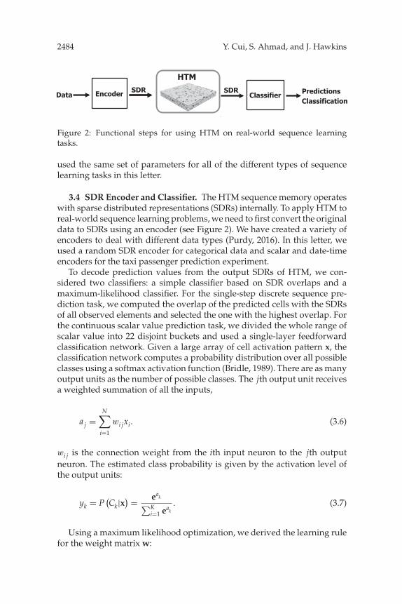
Figure 2: Functional steps for using HTM on real-world sequence learningtasks.

used the same set of parameters for all of the different types of sequencelearning tasks in this letter.

3.4 SDR Encoder and Classifier. The HTM sequence memory operateswith sparse distributed representations (SDRs) internally. To apply HTM toreal-world sequence learning problems, we need to first convert the originaldata to SDRs using an encoder (see Figure 2). We have created a variety ofencoders to deal with different data types (Purdy, 2016). In this letter, weused a random SDR encoder for categorical data and scalar and date-timeencoders for the taxi passenger prediction experiment.

To decode prediction values from the output SDRs of HTM, we con-sidered two classifiers: a simple classifier based on SDR overlaps and amaximum-likelihood classifier. For the single-step discrete sequence pre-diction task, we computed the overlap of the predicted cells with the SDRsof all observed elements and selected the one with the highest overlap. Forthe continuous scalar value prediction task, we divided the whole range ofscalar value into 22 disjoint buckets and used a single-layer feedforwardclassification network. Given a large array of cell activation pattern x, theclassification network computes a probability distribution over all possibleclasses using a softmax activation function (Bridle, 1989). There are as manyoutput units as the number of possible classes. The jth output unit receivesa weighted summation of all the inputs,

a j =N∑

i=1

wi jxi. (3.6)

wi j is the connection weight from the ith input neuron to the jth outputneuron. The estimated class probability is given by the activation level ofthe output units:

yk = P(Ck|x

) = eak∑Ki=1 eak

. (3.7)

Using a maximum likelihood optimization, we derived the learning rulefor the weight matrix w:


�wi j = −λ(y j − z j)xi. (3.8)

z j is the observed (target) distribution and λ is the learning rate. Note thatsince x is highly sparse, we only need to update a very small fraction ofthe weight matrix at any time. Therefore, the learning algorithm for theclassifier is fast despite the high dimensionality of the weight matrix.

4 High-Order Sequence Prediction with Artificial Data

We conducted experiments to test whether the HTM sequence mem-ory model, online sequential extreme learning machine (OS-ELM), time-delayed neural network (TDNN), and LSTM network are able to learnhigh-order sequences in an online manner, recover after modification tothe sequences, and make multiple predictions simultaneously. LSTM rep-resents the state-of-the-art recurrent neural network model for sequencelearning tasks (Graves 2012; Hochreiter & Schmidhuber, 1997). OS-ELM isa feedforward neural network model that is widely used for time-seriespredictions (Huang, Wang, & Lan, 2011; Wang & Han, 2014). TDNN is aclassical feedforward neural network designed to work with sequential data(Waibel et al., 1989). LSTM and HTM use the current pattern only as inputand are able to learn the high-order structure. ELM and TDNN require theuser to determine the number of steps to use as temporal context.

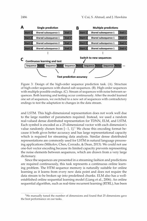
4.1 Continuous Online Learning from Streaming Data. We createda discrete high-order temporal sequence data set. Sequences are designedsuch that any learning algorithm would have to maintain context of at leastthe first two elements of each sequence in order to correctly predict the lastelement of the sequence (see Figure 3). We used the sequence data set in acontinuous streaming scenario (see Figure 3C). At the beginning of a trial,we randomly chose a sequence from the data set and sequentially presentedeach of its elements. At the end of each sequence, we presented a single noiseelement to the model. The noise element is randomly chosen from a largeset of 50,000 noise symbols (not used among the set of sequences). This is adifficult learning problem, since sequences are embedded in random noise;the start and end points are not marked. The set of noise symbols is largeso the algorithm cannot learn every possible noise transition. We tested thealgorithms for predicting the last element of each sequence continuously asthe algorithm observed a stream of sequences and reported the percentageof correct predictions over time.

We encoded each symbol in the sequence as a random SDR for HTMsequence memory, with 40 randomly chosen active bits in a vector of 2048bits. This SDR representation matches the internal representation used inHTM, which has 2048 columns with 40 active at any time (see the ap-pendix). We initially tried to use the same SDR encoding for TDNN, ELM,


Figure 3: Design of the high-order sequence prediction task. (A). Structureof high-order sequences with shared sub-sequences. (B). High-order sequenceswith multiple possible endings. (C). Stream of sequences with noise between se-quences. Both learning and testing occur continuously. After the model learnedone set of sequences, we switched to a new set of sequences with contradictoryendings to test the adaptation to changes in the data stream.

and LSTM. This high-dimensional representation does not work well dueto the large number of parameters required. Instead, we used a randomreal-valued dense distributed representation for TDNN, ELM, and LSTM.Each symbol is encoded as a 25-dimensional vector with each dimension’svalue randomly chosen from [−1, 1].1 We chose this encoding format be-cause it both gives better accuracy and has large representational capacitywhich is required for streaming data analysis. Similar dense distributedrepresentations are commonly used for LSTM in natural language process-ing applications (Mikolov, Chen, Corrado, & Dean, 2013). We could not useone-hot vector encoding because its limited capacity prevents representingthe noise elements between sequences, which are drawn from a very largedictionary.

Since the sequences are presented in a streaming fashion and predictionsare required continuously, this task represents a continuous online learn-ing problem. The HTM sequence memory is naturally suitable for onlinelearning as it learns from every new data point and does not require thedata stream to be broken up into predefined chunks. ELM also has a well-established online sequential learning model (Liang et al., 2006). An onlinesequential algorithm, such as real-time recurrent learning (RTRL), has been

1We manually tuned the number of dimensions and found that 25 dimensions gavethe best performance on our tasks.


proposed for LSTM in the past (Hochreiter & Schmidhuber, 1997; Williams& Zipser, 1989). However, most LSTM applications used batch learning dueto the high computational cost of RTRL (Jaeger, 2002). We use two variantsof LSTM networks for this task. First, we retrained an LSTM network atregular intervals on a buffered data set of the previous time steps using avariant of the resilient backpropagation algorithm until convergence (Igel &Husken, 2003). The experiments include several LSTM models with varyingbuffer sizes. Second, we trained an LSTM network with online truncatedbackpropagation through time (BPTT) (Williams & Peng, 1990). At each timepoint, we calculated the gradient using BPTT over the last 100 elements andadjusted the parameters along the gradient by a small amount.

We tested sequences with either single or multiple possible endings (seeFigures 3A and 3B). To quantify model performance, we classified the stateof the model before presenting the last element of each sequence to retrievethe top K predictions, where K = 1 for the single prediction case and K = 2or 4 for the multiple predictions case. We considered the prediction correctif the actual last element was among the top K predictions of the model.Since these are online learning tasks, there are no separate training and testphases. Instead, we continuously report the prediction accuracy of the endof each sequence before the model has seen it.

In the single prediction experiment (see Figure 4, left of the black solidline), each sequence in the data set has only one possible ending given itshigh-order context (see Figure 3A). The HTM sequence memory quicklyachieves perfect prediction accuracy on this task (see Figure 4, red). Given alarge enough learning window, LSTM also learns to predict the high-ordersequences (see Figure 4, green). Despite comparable model performance,HTM and LSTM use the data in different ways: LSTM requires many passesover the learning window—each time it is retrained to perform gradient-descent optimization, whereas HTM needs to see each element only once(one-pass learning). LSTM also takes longer than HTM to achieve perfectaccuracy; we speculate that since LSTM optimizes over all transitions in thedata stream, including the random ones between sequences, it is initiallyoverfitting on the training data. Online LSTM and ELM are also trained inan online, sequential fashion similar to HTM. But both algorithms requirekeeping a short history buffer of the past elements. ELM learned the se-quences more slowly than HTM and never achieved perfect performance(see Figure 4, blue). Online LSTM has the best performance initially, butdoes not achieve perfect performance in the end. HTM, LSTM, and TDNNare able to achieve perfect prediction accuracy on this task.2

2For TDNN, the user has to know the length of temporal context ahead of time inorder to obtain perfect performance. The results in Figure 3 used a lag of 10 steps. Wecould not obtain perfect performance with a lag of 5 or 20 steps.


Figure 4: Prediction accuracy of HTM (red), LSTM (yellow, green, purple), ELM(blue), and TDNN (cyan) on an artificial data set. The data set contains foursixth order sequences and four seventh order sequences. Prediction accuracyis calculated as a moving average over the last 100 sequences. The sequencesare changed after 10,000 elements have been seen (black dashed line). HTMsees each element once and learns continuously. ELM is trained continuouslyusing a time lag of 10 steps. TDNN is retrained every 1000 elements (orangevertical lines) on the last 1000 elements (cyan). LSTM is either retrained every1000 elements on the last 1000 elements (yellow) or 9000 elements (green), orcontinuously adapted using truncated BPTT (purple).

4.2 Adaptation to Changes in the Data Stream. Once the models haveachieved stable performance, we altered the data set by swapping the lastelements of pairs of high-order sequences (see Figure 4, black dashed line).This forces the model to forget the old sequences and subsequently learnthe new ones. HTM sequence memory and online LSTM quickly recoverfrom the modification. In contrast, it takes a long time for batch LSTM,TDNN, and ELM to recover from the modification as its buffered dataset contains contradictory information before and after the modification.Although using a smaller learning window can speed up the recovery (seeFigure 4, blue purple), it also causes worse prediction performance due tothe limited number of training samples.

A summary of the model performance on the high-order sequence pre-diction task is shown in Figure 5. In general, there is a trade-off betweenprediction accuracy and flexibility. For batch learning algorithms, a shorterlearning window is required for fast adaptation to changes in the data, but alonger learning window is required to perfectly learn high-order sequences


Figure 5: Final prediction accuracy as a function of the number of samplesrequired to achieve final accuracy before (left) and after (right) modification ofthe sequences. Error bars represent standard deviations.

(see Figure 5, green versus yellow). Although online LSTM and ELM donot require batch learning, the user is required to specify the maximal lag,which limits the maximum sequence order it can learn. The HTM sequencememory model dynamically learns high-order sequences without requir-ing a learning window or a maximum sequence length. It achieved the bestfinal prediction accuracy with a small number of data samples. After themodification to the sequences, HTM’s recovery is much faster than ELMand LSTM trained with batch learning, demonstrating its ability to adaptquickly to changes in data streams.

4.3 Simultaneous Multiple Predictions. In the experiment with mul-tiple predictions (see Figure 3B), each sequence in the data set has twoor four possible endings, given its high-order context. The HTM sequencememory model rapidly achieves perfect prediction accuracy for both the 2-predictions and the 4-predictions cases (see Figure 6). While only these twocases are shown, in reality HTM is able to make many multiple predictionscorrectly if the data set requires it. Given a large learning window, LSTMis able to achieve good prediction accuracy for the 2-predictions case, butwhen the number of predictions is increased to 4 or greater, it is not able tomake accurate predictions.

HTM sequence memory is able to simultaneously make multiple pre-dictions due to its use of SDRs. Because there is little overlap between tworandom SDRs, it is possible to predict a union of many SDRs and clas-sify a particular SDR as being a member of the union with low chance of a


Figure 6: Performance on high-order sequence prediction tasks that requiretwo (left) or four (right) simultaneous predictions. Shaded regions representstandard deviations (calculated with different sets of sequences). The data setcontains four sets of sixth order sequences and four sets of seventh-order se-quences.

false positive (Ahmad & Hawkins, 2016). On the other hand, the real-valueddense distributed encoding used in LSTM is not suitable for multiple predic-tions because the average of multiple dense representations in the encodingspace is not necessarily close to any of the component encodings, especiallywhen the number of predictions being made is large. The problem can besolved by using local one-hot representations to code target inputs, but suchrepresentations have very limited capacity and do not work well when thenumber of possible inputs is large or unknown upfront. This suggests thatmodifying LSTMs to use SDRs might enable better performance on thistask.

4.4 Learning Long Term Dependencies from High-Order Sequences.For feedforward networks like ELM, the number of time lags that canbe included in the input layer significantly limits the maximum sequenceorder a network can learn. The conventional recurrent neural networks can-not handle sequences with long-term dependencies because error signals“flowing backward in time” tend to either blow up or vanish with the clas-sical backpropagation-through-time (BPTT) algorithm. LSTM is capable oflearning very long-term dependencies using gating mechanisms (Henaff,Szlam, & Lecun, 2016). Here we tested whether HTM sequence memorycan learn long-term dependencies by varying the Markov order of the se-quences, which is determined by the length of shared sub-sequences (seeFigure 3A).

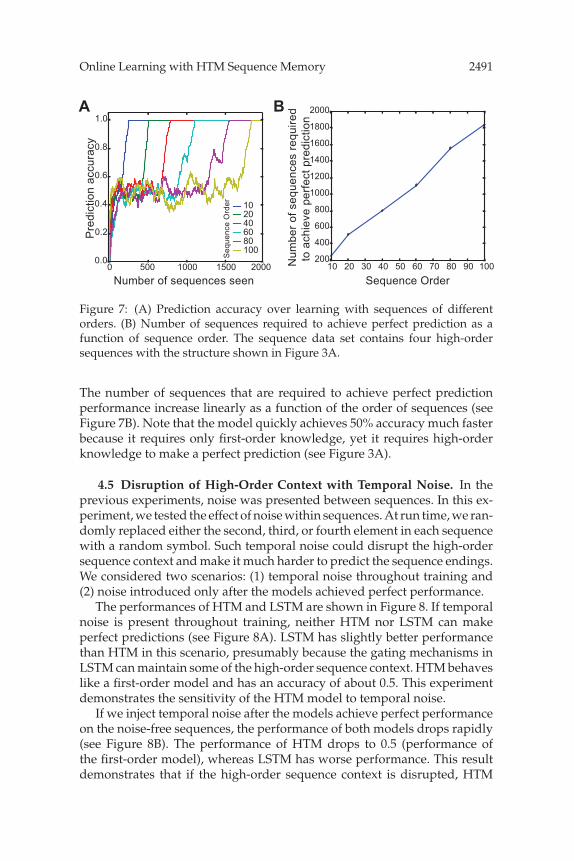
We examined the prediction accuracy over training while HTM sequencememory learns variable-order sequences. The model is able to achieve per-fect prediction performance up to 100-order sequences (see Figure 7A).


Figure 7: (A) Prediction accuracy over learning with sequences of differentorders. (B) Number of sequences required to achieve perfect prediction as afunction of sequence order. The sequence data set contains four high-ordersequences with the structure shown in Figure 3A.

The number of sequences that are required to achieve perfect predictionperformance increase linearly as a function of the order of sequences (seeFigure 7B). Note that the model quickly achieves 50% accuracy much fasterbecause it requires only first-order knowledge, yet it requires high-orderknowledge to make a perfect prediction (see Figure 3A).

4.5 Disruption of High-Order Context with Temporal Noise. In theprevious experiments, noise was presented between sequences. In this ex-periment, we tested the effect of noise within sequences. At run time, we ran-domly replaced either the second, third, or fourth element in each sequencewith a random symbol. Such temporal noise could disrupt the high-ordersequence context and make it much harder to predict the sequence endings.We considered two scenarios: (1) temporal noise throughout training and(2) noise introduced only after the models achieved perfect performance.

The performances of HTM and LSTM are shown in Figure 8. If temporalnoise is present throughout training, neither HTM nor LSTM can makeperfect predictions (see Figure 8A). LSTM has slightly better performancethan HTM in this scenario, presumably because the gating mechanisms inLSTM can maintain some of the high-order sequence context. HTM behaveslike a first-order model and has an accuracy of about 0.5. This experimentdemonstrates the sensitivity of the HTM model to temporal noise.

If we inject temporal noise after the models achieve perfect performanceon the noise-free sequences, the performance of both models drops rapidly(see Figure 8B). The performance of HTM drops to 0.5 (performance ofthe first-order model), whereas LSTM has worse performance. This resultdemonstrates that if the high-order sequence context is disrupted, HTM


Figure 8: (A) Prediction accuracy over learning with the presence of temporalnoise for LSTM (gray) and HTM (black). (B) HTM and LSTM are trained withclean sequences. Temporal noise was added after 12,000 elements. The sequencedata set is same as in Figure 4.

would robustly behave as a low-order model, whereas the performance ofLSTM is dependent on the training history.

4.6 Robustness of the Network to Damage. We tested the robustness ofthe ELM, LSTM, and HTM networks with respect to the removal of neurons.This fault tolerance property is important for hardware implementationsof neural network models. After the models achieved stable performanceon the high-order sequence prediction task (at the black dashed line, inFigure 2), we eliminated a fraction of the cells and their associated synapticconnections from the network. We then measured the prediction accuracyof both networks on the same data streams for an additional 5000 stepswithout further learning. There is no impact on the HTM sequence memorymodel performance at up to 30% cell death, whereas the performance ofthe ELM and LSTM networks declined rapidly with a small fraction of celldeath (see Figure 9).

Fault tolerance of traditional artificial neural networks depends on manyfactors, such as the network size and training methods (Lee, Hwang, &Sung, 2014). The experiments here applied commonly used training meth-ods for ELM and LSTM (see the appendix). It is possible that the faulttolerance of LSTM or any other artificial neural network may be improvedby introducing redundancy (replicating trained network) (Tchernev, Mul-vaney, & Phatak, 2005) or by a special training method such as dropout(Hinton, Krizhevsky, Sutskever, & Salakhutdinov, 2012). In contrast, thefault tolerance of HTM is naturally derived from properties of sparse


Figure 9: Robustness of the network to damage. The prediction accuracy aftercell death is shown as a function of the fraction of cells that were removed fromthe network.

distributed representations (Ahmad & Hawkins, 2016), in analogy to bi-ological neural networks.

5 Prediction of New York City Taxi Passenger Demand

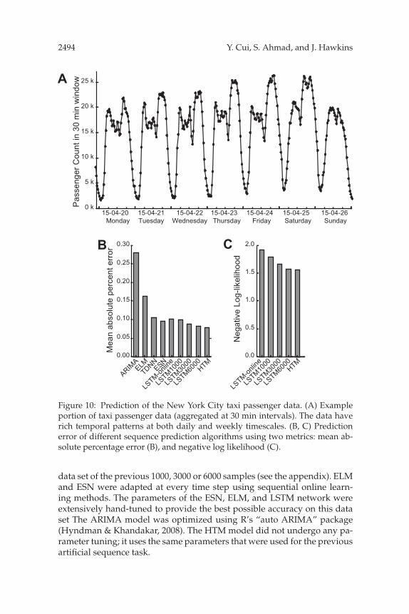
In order to compare the performance of HTM sequence memory with othersequence learning techniques in real-world scenarios, we consider the prob-lem of predicting taxi passenger demand. Specifically, we aggregated thepassenger counts in New York City taxi rides at 30 minute intervals us-ing a public data stream provided by the New York City TransportationAuthority.3 This leads to sequences exhibiting rich patterns at differenttimescales (see Figure 10A). The task is to predict taxi passenger demandfive steps (2.5 hours) in advance. This problem is an example of a large classof sequence learning problems that require rapid processing of streamingdata to deliver information for real-time decision making (Moreira-Matias,Gama, Ferreira, Mendes-Moreira, & Damas, 2013).

We applied HTM sequence memory and other sequence prediction al-gorithms to this problem. The ARIMA model is a widely used statisticalapproach for time series analysis (Hyndman & Athanasopoulos, 2013). Asbefore, we converted ARIMA, TDNN, and LSTM to an online learning al-gorithm by retraining the models on every week of data with a buffered

3http://www.nyc.gov/html/tlc/html/about/trip_record_data.shtml.


Figure 10: Prediction of the New York City taxi passenger data. (A) Exampleportion of taxi passenger data (aggregated at 30 min intervals). The data haverich temporal patterns at both daily and weekly timescales. (B, C) Predictionerror of different sequence prediction algorithms using two metrics: mean ab-solute percentage error (B), and negative log likelihood (C).

data set of the previous 1000, 3000 or 6000 samples (see the appendix). ELMand ESN were adapted at every time step using sequential online learn-ing methods. The parameters of the ESN, ELM, and LSTM network wereextensively hand-tuned to provide the best possible accuracy on this dataset The ARIMA model was optimized using R’s “auto ARIMA” package(Hyndman & Khandakar, 2008). The HTM model did not undergo any pa-rameter tuning; it uses the same parameters that were used for the previousartificial sequence task.


Figure 11: Prediction accuracy of LSTM and HTM after the introduction ofnew patterns. (A). The mean absolute percent error of HTM sequence memory(red) and LSTM networks (green, blue) after artificial manipulation of the data(black dashed line). The LSTM networks are retrained every week at the yellowvertical lines (B, C). Prediction error after the manipulation. HTM sequencememory has better accuracy on both the MAPE and the negative log-likelihoodmetrics.

We used two error metrics to evaluate model performance: mean abso-lute percentage error (MAPE) and negative log likelihood. The MAPE met-rics focus on the single best point estimation, while negative log likelihoodevaluates the models’ predicted probability distributions of future inputs(see appendix for details). We found that the HTM sequence memory hadcomparable performance to LSTM on both error metrics. Both techniqueshad a much lower error than ELM, ESN, and ARIMA (see Figure 10B). Notethat HTM sequence memory achieves this performance with a single-passtraining paradigm, whereas LSTM requires multiple passes on a buffereddata set.

We then tested how fast different sequence learning algorithms can adaptto changes in the data (see Figure 11). We artificially modified the data bydecreasing weekday morning traffic (7 a.m.–11 a.m.) by 20% and increasingweekday night traffic (9 p.m.–11 p.m.) by 20% starting from April 1, 2015.These changes in the data caused an immediate increase in prediction errorfor both HTM and LSTM (see Figure 11A). The prediction error of HTMsequence memory quickly dropped back in about two weeks, whereas theLSTM prediction error stayed high much longer. As a result, HTM sequencememory had better prediction accuracy than LSTM and other models afterthe data modification (see Figures 11B and 11C).

6 Discussion and Conclusions

In this letter, we have applied HTM sequence memory, a recently devel-oped neural network model, to real-time sequence learning problems with


time-varying input streams. The sequence memory model is derived fromcomputational principles of cortical pyramidal neurons (Hawkins & Ah-mad, 2016). We discussed model performance on both artificially generatedand real-world data sets. The model satisfies a set of properties that areimportant for online sequence learning from noisy data streams with con-tinuously changing statistics, a problem the cortex has to solve in naturalenvironments. These properties govern the overall flexibility of an algo-rithm and its ability to be used in an automated fashion. Although HTM isstill at a very early stage compared to other traditional neural network mod-els, it satisfies these properties and shows promising results on real-timesequence learning problems.

6.1 Continuous Learning with Streaming Data. Most supervised se-quence learning algorithms use a batch-training paradigm, where a costfunction, such as prediction error, is minimized on a batch training dataset (Bishop, 2006; Dietterich, 2002). Although we can train these algorithmscontinuously using a sliding window (Sejnowski & Rosenberg, 1987), thisbatch-training paradigm is not a good match for time-series predictionon continuous streaming data. A small window may not contain enoughtraining samples for learning complex sequences, while a large window in-troduces a limit on how fast the algorithm can adapt to changing statisticsin the data. In either case, a buffer must be maintained, and the algorithmmust make multiple passes for every retraining step. It may be possible touse a smooth forgetting mechanism instead of hard retraining (Lughofer &Angelov, 2011; Williams & Zipser, 1989), but this requires the user to tuneparameters governing the forgetting speed to achieve good performance.

In contrast, HTM sequence memory adopts a continuous learningparadigm. The model does not need to store a batch of data as the “train-ing dataset.” Instead, it learns from each data point using unsupervisedHebbian-like associative learning mechanisms (Hebb, 1949). As a result,the model rapidly adapts to changing statistics in the data.

6.2 Using Sparse Distributed Representations for Sequence Learning.A key difference between HTM sequence memory and previous biologicallyinspired sequence learning models (Abeles, 1982; Brea et al., 2013; Ponulak& Kasinski, 2010; Rao & Sejnowski, 2001) is the use of sparse distributedrepresentations (SDRs). In the cortex, information is primarily representedby strong activation of a small set of neurons at any time, known as sparsecoding (Foldiak 2002, Olshausen & Field, 2004). HTM sequence memoryuses SDRs to represent temporal sequences. Based on mathematical prop-erties of SDRs (Ahmad & Hawkins, 2016; Kanerva, 1988), each neuron inthe HTM sequence memory model can robustly learn and classify a largenumber of patterns under noisy conditions (Hawkins & Ahmad, 2016).A rich distributed neural representation for temporal sequences emergesfrom computation in HTM sequence memory. Although we focus on se-quence prediction in this letter, this representation is valuable for a number


of tasks, such as anomaly detection (Lavin & Ahmad, 2015) and sequenceclassification.

The use of a flexible coding scheme is particularly important for onlinestreaming data analysis, where the number of unique symbols is often notknown upfront. It is desirable to be able to change the range of the codingscheme at run time without affecting previous learning. This requires thealgorithm to use a flexible coding scheme that can represent a large numberof unique symbols or a wide range of data. The SDRs used in HTM havea very large coding capacity and allow simultaneous representations ofmultiple predictions with minimal collisions These properties make SDRan ideal coding format for the next generation of neural network models.

6.3 Robustness and Generalization. An intelligent learning algorithmshould be able to automatically deal with a large variety of problems with-out parameter tuning, yet most machine learning algorithms require a task-specific parameter search when applied to a novel problem. Learning in thecortex does not require an external tuning mechanism, and the same corti-cal region can be used for different functional purposes if the sensory inputchanges (Sadato et al., 1996; Sharma, Angelucci, & Sur, 2000). Using com-putational principles derived from the cortex, we show that HTM sequencememory achieves performance comparable to LSTM networks on very dif-ferent problems using the same set of parameters. These parameters werechosen according to known properties of real cortical neurons (Hawkins& Ahmad, 2016) and basic properties of sparse distributed representations(Ahmad & Hawkins, 2016).

6.4 Limitations of HTM and Future Directions. We have identified afew limitations of HTM. First, as a strict one-pass algorithm with accessto only the current input, it may take longer for HTM to learn sequenceswith very long-term dependencies (see Figure 7) than algorithms that haveaccess to a longer history buffer. Learning of sequences with long-termdependencies can be sped up if we maintain a history buffer and run HTMon it multiple times. Indeed, it has been argued that an intelligent agentshould store the entire raw history of sensory inputs and motor actionsduring interaction with the world (Schmidhuber, 2009). Although it maybe computationally challenging to store the entire history, doing so mayimprove performance given the same amount of sensory experience.

Second, although HTM is robust to spatial noise due to the use of sparsedistributed representations, the current HTM sequence memory model issensitive to temporal noise. It can lose high-order sequence context if el-ements in the sequence are replaced by a random symbol (see Figure 8).In contrast, the gating mechanisms of LSTM networks appear to be morerobust to temporal noise. The noise robustness of HTM can be improvedby using a hierarchy of sequence memory models that operate on differenttimescales. A sequence memory model that operates over longer timescales


would be less sensitive to temporal noise. A lower region in the hierarchymay inherit the robustness to temporal noise through feedback connectionsto a higher region.

Third, the HTM model as discussed does not perform as well as LSTMon grammar learning tasks. We found that on the Reber grammar task(Hochreiter & Schmidhuber, 1997), HTM achieves an accuracy of 98.4% andELM an accuracy of 86.7% (online training after observing 500 sequences),whereas LSTM achieves an accuracy of 100%. HTM can approximatelylearn artificial grammars by memorizing example sentences. This strategycould require more training samples to fully learn recursive grammars witharbitrary sequence lengths. In contrast, LSTM learns grammars much fasterusing the gating mechanisms. Unlike the HTM model, LSTMs can alsomodel some Boolean algebra problems like the parity problem.

Finally, we have tested HTM only on low-dimensional categorical orscalar data streams in this letter. It remains to be determined whether HTMcan handle high-dimensional data such as speech and video streams. Thehigh capacity of the sparse distributed representations in HTM should beable to represent high-dimensional data. However, it is more challenging tolearn sequence structure in high-dimensional space, as the raw data couldbe much less repeatable. It may require additional preprocessing, such asdimensionality reduction and feature extractions, before HTM can learnmeaningful sequences with high-dimensional data. It would be an interest-ing future direction to explore how to combine HTM with other machinelearning methods, such as deep networks, to solve high-dimensional se-quence learning problems.

Appendix: Implementation Details

A.1 HTM Sequence Model Implementation Details. In our softwareimplementation, we made a few simplifying assumptions to speed up sim-ulation for large networks. We did not explicitly initialize a complete set ofsynapses across every segment and every cell. Instead, we greedily createdsegments on the least-used cells in an unpredicted column and initializedpotential synapses on that segment by sampling from previously activecells. This happened only when there is no match to any existing segment.The initial synaptic permanence for newly created synapses is set as 0.21(see Table 1), which is below the connection threshold (0.5).

The HTM sequence model operates with sparse distributed representa-tions (SDRs). Specialized encoders are required to encode real-world datainto SDRs. For the artificial data sets with categorical elements, we simplyencoded each symbol in the sequence as a random SDR, with 40 randomlychosen active bits in a vector of 2048 bits.

For the New York City taxi data set, three pieces of information were fedinto the HTM model: raw passenger count, the time of day, and the dayof week (LSTM received the same information as input). We used NuPIC’s


Table 1: Model Parameters for HTM.

Parameter Name Value

Number of columns N 2048Number of cells per column M 32Dendritic segment activation threshold θ 15Initial synaptic permanence 0.21Connection threshold for synaptic permanence 0.5Synaptic permanence increment p+ 0.1Synaptic permanence decrement p− 0.1Synaptic permanence decrement for predicted inactive segments p− 0.01Maximum number of segments per cell 128Maximum number of synapses per segments 128Maximum number new synapses added at each step 32

standard scalar encoder to convert each piece of information into an SDR.The encoder converts a scalar value into a large binary vector with a smallnumber of ON bits clustered within a sliding window, where the centerposition of the window corresponds to the data value. We subsequentlycombined three SDRs via a competitive sparse spatial pooling process,which also resulted in 40 active bits in a vector of 2048 bits as in the artificialdata set. The spatial pooling process is described in detail in Hawkins et al.(2011).

The HTM sequence memory model used an identical set of model param-eters for all the experiments described in the letter. A complete list of modelparameters is shown below. The full source code for the implementation isavailable on Github at https://github.com/numenta/nupic.research.

A.2 Implementation Details of Other Sequence Learning Algorithms.

A.2.1 ELM. We used the online sequential learning algorithm for ELM(Liang et al., 2006). The network used 50 hidden neurons and a time lag of100 for the taxi data and 200 hidden neurons and a time lag of 10 for theartificial data set.

A.2.2 ESN. We used the Matlab toolbox for echo state network devel-oped by Jaeger’s group (http://reservoir-computing.org/node/129). TheESN network has 100 internal units, a spectral radius of 0.1, a teacher scal-ing of 0.01, and a learning rate of 0.1 for the ESN model. The parameters werehand-tuned to achieve the best performance. We used the online learningmode and adapted the weight at every time step.

A.2.3 LSTM. We used the PyBrain implementation of LSTM (Schaulet al., 2010). For the artificial sequence learning task, the network contains25 input units, 20 internal LSTM neurons, and 25 output units. For the NYCtaxi task, the network contains 3 input units, 20 LSTM cells, 1 output unit


for calculation of the MAPE metric, and 22 output units for calculation ofthe sequence likelihood metric. The LSTM cells have forget gates but notpeephole connections. The output units have a biased term. The maximumtime lag is the same as the buffer size for the batch-learning LSTMs. We usedtwo training paradigms. For the batch-learning paradigm, the networkswere retrained every 1000 iterations with a popular version of the resilientbackpropagation method (Igel & Husken 2003). For the online learningparadigm, we calculated the gradient at every time step using truncatedbackpropgation through time over the last 100 elements (Williams & Peng,1990), and adjusted the parameters along the gradient with a learning rateof 0.01.

A.2.4 TDNN. Time-delayed neural network was implemented as a sin-gle hidden layer feedforward neural network with time-delayed inputswith PyBrain. For the artificial data set, the network contains 250 inputunits (10 time lags × 25 dimensional input per time step), 200 hidden units,and 25 output units. For the taxi data, the network contains 100 input units(100 time labs), 200 hidden units, and 1 output unit. We included bias forboth input and output units in both cases. The networks were retrainedevery 1000 iterations (artificial data set) or every 336 iterations (taxi data)on the past 3000 data records using standard backpropagation.

A.3 Evaluation of Model Performance in the Continuous SequenceLearning Task. Two error metrics were used to evaluate the predictionaccuracy of the model. First, we considered the mean absolute percentageerror (MAPE) metric, an error metric that is less sensitive to outliers thanroot mean squared error:

MAPE =∑N

t=1 |yt − yt |∑Nt=1 |yt |

. (A.1)

In equation A.1, yt is the observed data at time t, yt is the model predictionfor the data observed at time t, and N is the length of the data set.

A good prediction algorithm should output a probability distribution offuture elements of the sequence. However, MAPE, consider only the singlebest prediction from the model and thus does not incorporate other possiblepredictions from the model. We used negative log likelihood as a comple-mentary error metric to address this problem. The sequence probability canbe decomposed into

p(y1, y2, . . . , yt ) = p(y1)p(y2|y1)p(y3|y1, y2)p(yt |y1, . . . , yt−1). (A.2)

The conditional probability distribution is modeled by HTM or LSTMbased on network state at the previous time step:


p(yt |y1, . . . , yt−1) = P(yt |network statet−1). (A.3)

The negative log likelihood of the sequence is then given by

NLL = 1N

N∑t=1

log P(yt |model). (A.4)

Acknowledgments

We thank the NuPIC open source community (numenta.org) for continuoussupport and enthusiasm about HTM. We thank the reviewers for numeroussuggestions that significantly improved the overall letter. We also thankChetan Surpur for helping to run some of the simulations and our Numentacolleagues for many helpful discussions.

References

Abeles, M. (1982). Local cortical circuits: An electrophysiological study. Berlin: Springer.Ahmad, S., & Hawkins, J. (2016). How do neurons operate on sparse distributed representa-

tions? A mathematical theory of sparsity, neurons and active dendrites. arXiv.1601.00720Antic, S. D., Zhou, W. L., Moore, A. R., Short, S. M., & Ikonomu, K. D. (2010). The

decade of the dendritic NMDA spike. J. Neurosci. Res., 88, 2991–3001.Ben Taieb, S., Bontempi, G., Atiya, A. F., & Sorjamaa, A. (2012). A review and com-

parison of strategies for multi-step ahead time series forecasting based on theNN5 forecasting competition. Expert Syst. Appl., 39(8), 7067–7083.

Bishop, C. (2006). Pattern recognition and machine learning. Singapore: Springer.Brea, J., Senn, W., & Pfister, J.-P. (2013). Matching recall and storage in sequence

learning with spiking neural networks. J. Neurosci., 33(23), 9565–9575.Bridle, J. (1989). Probabilistic interpretation of feedforward classification network

outputs, with relationships to statistical pattern recognition. In F. Fogelman Soulie& J. Heravlt (Eds.), Neurocomputing: Algorithms, architectures and applications (pp.227–236). Berlin: Springer-Verlag.

Brosch, M., & Schreiner, C. E. (2000). Sequence sensitivity of neurons in cat primaryauditory cortex. Cereb. Cortex., 10(12), 1155–1167.

Buxhoeveden, D. P. (2002). The minicolumn hypothesis in neuroscience. Brain, 125(5),935–951.

Clegg, B. A., Digirolamo, G. J., & Keele, S. W. (1998). Sequence learning. Trends Cogn.Sci. 2(8), 275–281.

Crone, S. F., Hibon, M., & Nikolopoulos, K. (2011). Advances in forecasting withneural networks? Empirical evidence from the NN3 competition on time seriesprediction. Int. J. Forecast., 27(3), 635–660.

Dietterich, T. G. (2002). Machine learning for sequential data: A review. In Proceedingsof the Jt. IAPR Int. Work. Struct. Syntactic, Stat. Pattern Recognition (pp. 15–30).Berlin: Springer-Verlag.


Domingos, P., & Hulten, G. (2000). Mining high-speed data streams. Proceedings ofthe Sixth ACM SIGKDD Int. Conf. Knowl. Discov. Data Mining (pp. 71–80). NewYork: ACM Press.

Durbin, J., & Koopman, S. J. (2012). Time series analysis by state space methods (2nded.). New York: Oxford University Press.

Fine, S., Singer, Y., & Tishby, N. (1998). The hierarchical hidden markov model:Analysis and applications. Mach. Learn., 32(1), 41–62.

Foldiak, P. (2002). Sparse coding in the primate cortex. In M. A. Arbib (Ed.), Thehandbook of brain theory and neural networks ( 2nd ed.), (pp. 1064–1068). Cambridge,MA: MIT Press.

Gaber, M. M., Zaslavsky, A., & Krishnaswamy, S. (2005). Mining data streams. ACMSIGMOD Rec., 34(2), 18.

Gama, J. (2010). Knowledge discovery from data streams. Boca Raton, FL: Chapman andHall/CRC.

Gavornik, J. P., & Bear M. F. (2014). Learned spatiotemporal sequence recognitionand prediction in primary visual cortex. Nat. Neurosci., 17, 732–737.

Graves, A. (2012). Supervised sequence labelling with recurrent neural networks. NewYork: Springer.

Greff, K., Srivastava, R., Koutnik, J., Steunebrink, B. R., & Schmidhuber, J. (2015).LSTM: A search space Odyssey. arXiv.1503.04069

Hawkins, J., & Ahmad, S. (2016). Why neurons have thousands of synapses: A theoryof sequence memory in neocortex. Front. Neural Circuits, 10.

Hawkins, J., Ahmad, S., & Dubinsky, D. (2011). Cortical learning algorithm and hier-archical temporal memory. Numenta white paper. http://numenta.org/resources/HTM_CorticalLearningAlgorithms.pdf

Hebb, D. (1949). The organization of behavior: A neuropsychological theory. Sci.Educ., 44(1), 335.

Henaff, M., Szlam, A., & Lecun, Y. (2016). Orthogonal RNNs and long-memory tasks.arXiv.1602.06662

Hinton, G., Srivastava, N., Krizhevsky, A., Sutskever, I., & Salakhutdinov, R.(2012). Improving neural networks by preventing co-adaptation of feature detectors.arXiv.1207.0580

Hochreiter, S., & Schmidhuber, J. (1997). Long short-term memory. Neural Comput.,9(8), 1735–1780.

Huang, G.-B., Wang, D. H., & Lan, Y. (2011). Extreme learning machines: A survey.Int. J. Mach. Learn. Cybern., 2(2), 107–122.

Huang, G.-B., Zhu, Q.-Y., & Siew, C.-K. (2006). Extreme learning machine: Theoryand applications. Neurocomputing, 70, 489–501.

Hyndman, R. J., & Athanasopoulos, G. (2013). Forecasting: Principles and practice.OTexts, https://www.otexts.org/fpp.

Hyndman, R. J., & Khandakar, Y. (2008). Automatic time series forecasting: Theforecast package for R. J. Stat. Softw., 26(3).

Igel, C., & Husken, M. (2003). Empirical evaluation of the improved Rprop learningalgorithms. Neurocomputing, 50, 105–123.

Jaeger, H. (2002). Tutorial on training recurrent neural networks, covering BPPT, RTRL,EKF and the “echo state network” approach (GMD Rep. 159. 48). Hanover: GermanNational Research Center for Information Technology.

http://numenta.org/resources/HTM_CorticalLearningAlgorithms.pdf

http://numenta.org/resources/HTM_CorticalLearningAlgorithms.pdf


Jaeger, H., & Haas, H. (2004). Harnessing nonlinearity: Predicting chaotic systemsand saving energy in wireless communication. Science, 304(5667), 78–80.

Kanerva, P. (1988). Sparse distributed memory. Cambrige, MA: MIT Press.Lavin, A., & Ahmad, S. (2015). Evaluating real-time anomaly detection algorithms:

The Numenta anomaly benchmark. In Proceedings of the 14th Int. Conf. Mach. Learn.Appl. Piscataway, NJ: IEEE.

LeCun, Y., Bengio, Y., & Hinton, G. (2015). Deep learning. Nature, 521(7553), 436–444.

Lee, M., Hwang, K., & Sung, W. (2014). Fault tolerance analysis of digital feedforwarddeep neural networks. In Proceedings of the 2014 IEEE Int. Conf. Acoust. SpeechSignal Processing, (pp. 5031–5035). Piscataway, NJ: IEEE.

Liang, N.-Y., Huang, G.-B., Saratchandran, P., & Sundararajan, N. (2006). A fast andaccurate online sequential learning algorithm for feedforward networks. IEEETrans. Neural Netw., 17(6), 1411–1423.

Lipton, Z. C., Berkowitz, J., & Elkan, C. (2015). A critical review of recurrent neuralnetworks for sequence learning. arXiv.1506.00019[cs.LG]

Lughofer, E., & Angelov, P. (2011). Handling drifts and shifts in on-line data streamswith evolving fuzzy systems. Appl. Soft Comput., 11(2), 2057–2068.

Major, G., Larkum, M. E., & Schiller, J. (2013). Active properties of neocortical pyra-midal neuron dendrites. Annu. Rev. Neurosci., 36 1–24.

Massey, P. V., & Bashir, Z. I. (2007). Long-term depression: Multiple forms andimplications for brain function. Trends Neurosci., 30(4), 176–184.

Mauk, M. D., & Buonomano, D. V. (2004). The neural basis of temporal processing.Annu. Rev. Neurosci., 27, 307–340.

McFarland, J. M., Cui, Y., & Butts, D. A. (2013). Inferring nonlinear neuronal computa-tion based on physiologically plausible inputs. PLoS Comput. Biol., 9(7), e1003143.

Mikolov, T., Chen, K., Corrado, G., & Dean, J. (2013). Efficient estimation of wordrepresentations in vector space. arXiv.1301.3781

Mnatzaganian, J., Fokoue, E., & Kudithipudi, D. (2016). A mathematical formalizationof hierarchical temporal memory’s spatial pooler. arXiv.1601.06116.

Moreira-Matias, L., Gama, J., Ferreira, M., Mendes-Moreira, J., & Damas, L. (2013).Predicting taxi–passenger demand using streaming data. IEEE Trans. Intell.Transp. Syst., 14(3), 1393–1402.

Mountcastle, V. B. (1997). The columnar organization of the neocortex. Brain, 120 (Pt.4), 701–722.

Nikolic, D., Hausler, S., Singer, W., & Maass, W. (2009). Distributed fading memoryfor stimulus properties in the primary visual cortex. PLoS Biol., 7(12), e1000260.

Olshausen, B. A., & Field, D. J. (2004). Sparse coding of sensory inputs. Curr. Opin.Neurobiol., 14, 481–487.

Polsky, A., Mel, B. W., & Schiller, J. (2004). Computational subunits in thin dendritesof pyramidal cells. Nat. Neurosci., 7(6), 621–627.

Ponulak, F., & Kasinski, A. (2010). Supervised learning in spiking neural networkswith ReSuMe: Sequence learning, classification, and spike shifting. Neural Com-put., 22(2), 467–510.

Purdy, S. (2016). Encoding data for HTM systems. arXiv.1602.05925Rabiner, L., & Juang, B. (1986). An introduction to hidden Markov models. IEEE

ASSP Mag., 3(1), 4–16.


Rao, R. P., & Sejnowski, T. J. (2001). Predictive learning of temporal sequences inrecurrent neocortical circuits. In Proceedings of the Novartis Found. Symp., 239, (pp.208–229; discussion 229–240).

Sadato, N., Pascual-Leone, A., Grafman, J., Ibanez, V., Deiber, M. P., & Hallett, M.(1996). Activation of the primary visual cortex by Braille reading in blind subjects.Nature, 380(6574), 526–528.

Sayed-Mouchaweh, M., & Lughofer, E. (2012). Learning in non-stationary environ-ments: Methods and applications. New York: Springer.

Schaul, T., Bayer, J., Wierstra, D., Sun, Y., Felder, M., Sehnke, F., . . . Schmidhuber, J.(2010). PyBrain. J. Mach. Learn. Res. 11, 743–746.

Schmidhuber, J. (2009). Simple algorithmic theory of subjective beauty, novelty,surprise, interestingness, attention, curiosity, creativity, art, science, music, jokes.Journal of the Society of Instrument and Control Engineers, 48(1), 21–32.

Schmidhuber, J. (2014). Deep learning in neural networks: An overview. NeuralNetworks, 61, 85–117.

Sejnowski, T., & Rosenberg, C. (1987). Parallel networks that learn to pronounceEnglish text. J. Complex Syst., 1(1), 145–168.

Sharma, J., Angelucci, A., & Sur, M. (2000). Induction of visual orientation modulesin auditory cortex. Nature, 404(6780), 841–847.

Smith, S. L., Smith, I. T, Branco, T., & Hausser, M. (2013). Dendritic spikes enhancestimulus selectivity in cortical neurons in vivo. Nature, 503(7474), 115–120.

Spruston, N. (2008). Pyramidal neurons: Dendritic structure and synaptic integra-tion. Nat. Rev. Neurosci., 9(3), 206–221.

Sutskever, I., Vinyals, O., & Le, Q. V. (2014). Sequence to sequence learning withneural networks. In Z. Ghahramani, M. Welling, C. Cortes, N. D. Lawrence, &K. Q. Weinberger (Eds.), Advances in neural information processing systems, 27 (pp.3104–3112). Red Hook, NY: Curran.

Tchernev, E. B., Mulvaney, R. G., & Phatak, D. S. (2005). Investigating the faulttolerance of neural networks. Neural Comput., 17(7), 1646–1664.

Tran, A. H., Yanushkevich, S. N., Lyshevski, S. E., & Shmerko, V. P. (2011). Design ofneuromorphic logic networks and fault-tolerant computing. In Proceedings of the2011 11th IEEE Int. Conf. Nanotechnology, (pp. 457–462). Piscataway, NJ: IEEE.

Waibel, A., Hanazawa, T., Hinton, G., Shikano, K., & Lang, K. J. (1989). Phonemerecognition using time-delay neural networks. IEEE Trans. Acoust., 37(3), 328–339.

Wang, X., & Han, M. (2014). Online sequential extreme learning machine with kernelsfor nonstationary time series prediction. Neurocomputing, 145, 90–97.

Williams, R. J., & Peng, J. (1990). An efficient gradient-based algorithm for on-linetraining of recurrent network trajectories. Neural Comput., 2(4), 490–501.

Williams, R. J., & Zipser, D. (1989). A learning algorithm for continually runningfully recurrent neural networks. Neural Comput., 1(2), 270–280.

Xu, S., Jiang, W., Poo, M.-M., & Dan, Y. (2012). Activity recall in a visual corticalensemble. Nat. Neurosci., 15(3), 449–455, S1–S2.

Zito, K., & Svoboda, K. (2002). Activity-dependent synaptogenesis in the adult Mam-malian cortex. Neuron, 35(6), 1015–1017.

Received December 10, 2015; accepted July 11, 2016.

continuous online sequence learning with an unsupervised ...€¦ · continuous online sequence...

Documents