continuous distributions for any x, p(x=x)=0. (for a continuous distribution, the area under a point...
TRANSCRIPT

Continuous distributions For any x, P(X=x)=0. (For a
continuous distribution, the area under a point is 0.)
Can’t use P(X=x) to describe the probability distribution of X
Instead, consider P(a≤X≤b)

Density function
A curve f(x): f(x) ≥ 0 The area under the
curve is 1
P(a≤X≤b) is the area between a and b
0 2 4 6 8 10
x
0.00
0.05
0.10
0.15
0.20
0.25
y

P(2≤X≤4)= P(2≤X<4)= P(2<X<4)
0 2 4 6 8 10
x
0.00
0.05
0.10
0.15
0.20
0.25
y

The normal distribution A normal curve: Bell shaped Density is given by
μand σ2 are two parameters: mean and standard variance of a normal population
(σ is the standard deviation)
2
2
1 ( )( ) exp
22
xf x
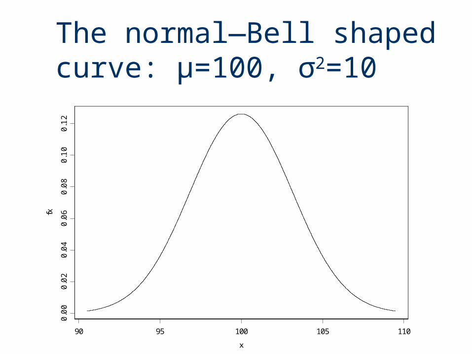
The normal—Bell shaped curve: μ=100, σ2=10
90 95 100 105 110
x
0.00
0.02
0.04
0.06
0.08
0.10
0.12
fx

Normal curves:(μ=0, σ2=1) and (μ=5, σ 2=1)
-2 0 2 4 6 8
x
0.0
0.1
0.2
0.3
0.4
fx1

Normal curves:(μ=0, σ2=1) and (μ=0, σ2=2)
-3 -2 -1 0 1 2 3
x
0.0
0.1
0.2
0.3
0.4
y

Normal curves:(μ=0, σ2=1) and (μ=2, σ2=0.25)
-2 0 2 4 6 8
x
0.0
0.2
0.4
0.6
0.8
1.0
fx1
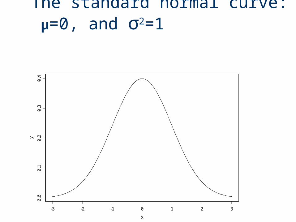
The standard normal curve: μ=0, and σ2=1
-3 -2 -1 0 1 2 3
x
0.0
0.1
0.2
0.3
0.4
y

How to calculate the probability of a normal random variable?
Each normal random variable, X, has a density function, say f(x) (it is a normal curve).
Probability P(a<X<b) is the area between a and b, under the normal curve f(x)
Table A.1(Appendix A, page 812) in the back of the book gives areas for a standard normal curve with =0 and =1.
Probabilities for any normal curve (any and ) can be rewritten in terms of a standard normal curve.

Normal-curve Areas Areas under standard normal curve Areas between 0 and z (z>0) How to get an area between a and
b? when a<b, and a, b positive area[0,b]–area[0,a]

Get the probability from standard normal table z denotes a standard normal
random variable Standard normal curve is symmetric
about the origin 0 Draw a graph
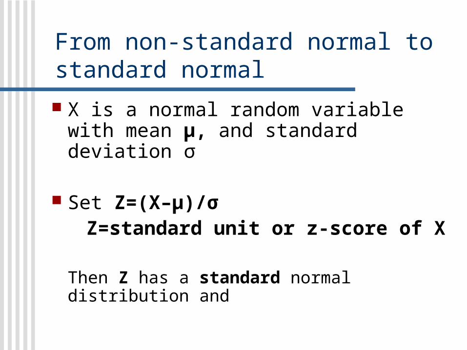
From non-standard normal to standard normal
X is a normal random variable with mean μ, and standard deviation σ
Set Z=(X–μ)/σ Z=standard unit or z-score of X
Then Z has a standard normal distribution and

Table A.1: P(0<Z<z) page 812
z .00 .01 .02 .03 .04 .05 .06 0.0 .0000 .0040 .0080 .0120 .0160 .0199 .02390.1 .0398 .0438 .0478 .0517 .0557 .0596 .0636 0.2 .0793 .0832 .0871 .0910 .0948 .0987 .10260.3 .1179 .1217 .1255 .1293 .1331 .1368 .1404 0.4 .1554 .1591 .1628 .1664 .1700 .1736 .1772 0.5 .1915 .1950 .1985 .2019 .2054 .2088 .2123… … … … … … … …1.0 .3413 .3438 .3461 .3485 .3508 .3531 .3554 1.1 .3643 .3665 .3686 .3708 .3729 .3749 .3770

Examples
Example 1 P(0<Z<1)= 0.3413 Example 2 P(1<Z<2)=P(0<Z<2)–P(0<Z<1)=0.4772–0.3413=0.1359
Adobe Acrobat 7.0 Document

Examples
Example 3 P(Z≥1) =0.5–P(0<Z<1) =0.5–0.3413 =0.1587
Adobe Acrobat 7.0 Document
Examples
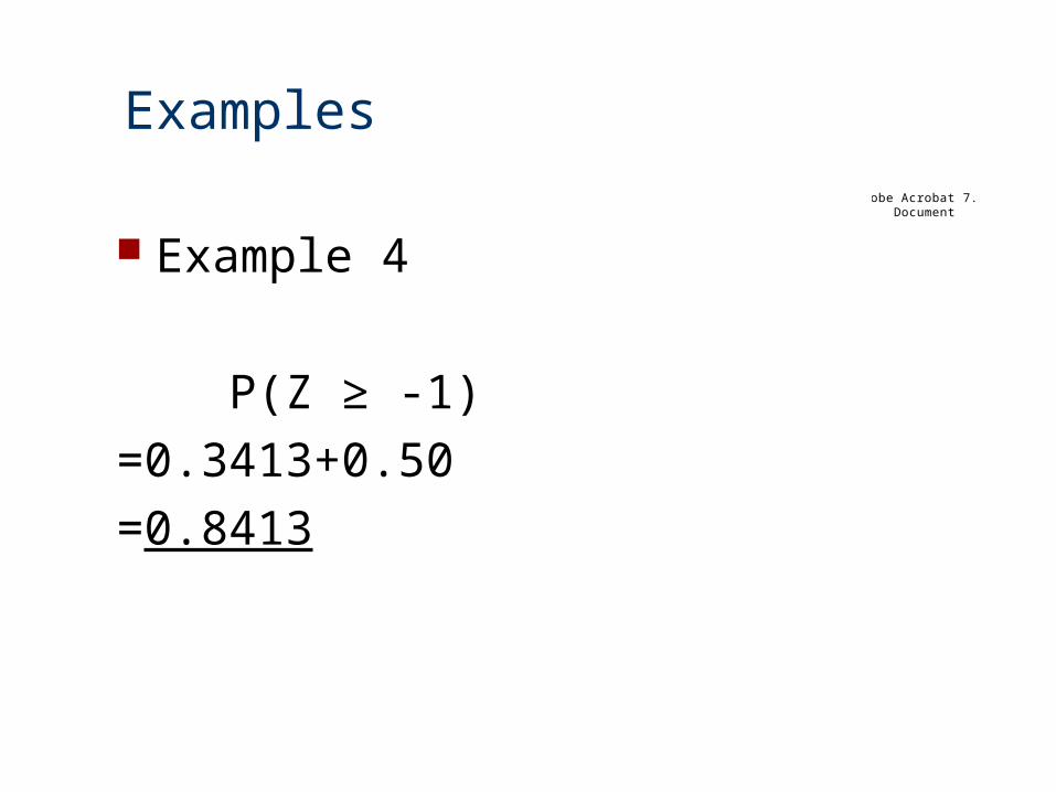
Example 4
P(Z ≥ -1)=0.3413+0.50=0.8413
Adobe Acrobat 7.0 Document

Examples
Example 5
P(-2<Z<1)=0.4772+0.3413=0.8185
Adobe Acrobat 7.0 Document

Examples
Example 6
P(Z ≤ 1.87)=0.5+P(0<Z ≤ 1.87)=0.5+0.4693=0.9693
Adobe Acrobat 7.0 Document

Examples
Example 7
P(Z<-1.87)= P(Z>1.87)= 0.5–0.4693= 0.0307
Adobe Acrobat 7.0 Document

Example 8
X is a normal random variablewith μ=120, and σ=15 Find the probability P(X≤135)Solution:
120
15120 120
015
15 1
15135 120
( 135) ( ) ( 1) 0.5 0.3413 0.841315
z
z
x xLet z
z is normal
xP x P P z

XZ x z-score of xExample 8 (continued)
P(X≤150)x=150 z-score z=(150-120)/15=2 P(X≤150)=P(Z≤2)= 0.5+0.4772= 0.9772