continuous and categorical independent variables-i: attribute … · continuous and categorical...
TRANSCRIPT
Continuous and Categorical Independent Variables-I:
Attribute-Treatment Interaction; Comparing Regression Equations
Chapter 14

● Previous techniques used either
Categorical Independent Variables or Continuous Independent Variables
● Now, we will look at techniques when we have both Categorical and Continuous Independent Variables together

Example● An experiment was designed to study the
effects of incentive and study time on retention
● Design:– 2 Groups of Subjects: Incentive, No Incentive
● This is a categorical variable– Amount of study time: 5, 10, 15, 20
● Time can be thought of as a continuous variable– Dependent variable was score on test
(retention)● A continuous dependent variable

Incentives...

Study Time...

Test

How can we analyze?● One way: Compute two regression lines,
one for the Incentive Group and one for the No Incentive Group.
● Then, look to see how these two lines differ (if at all).

Two Regression Lines
Incentive GroupRetention = 7.33330 + .20667*Study Time
No Incentive GroupRetention = 2.49996 + .26667*Study Time
Simply by glancing at these two equations, you can notice where the differences may lie…..

Compare Slopes
Incentive GroupRetention = 7.33330 + .20667*Study Time
No Incentive GroupRetention = 2.49996 + .26667*Study Time
.20667 is fairly close to .26667The slopes don’t seem that differentThe increase in test score as a function of study time is
very similar in both incentive groups.
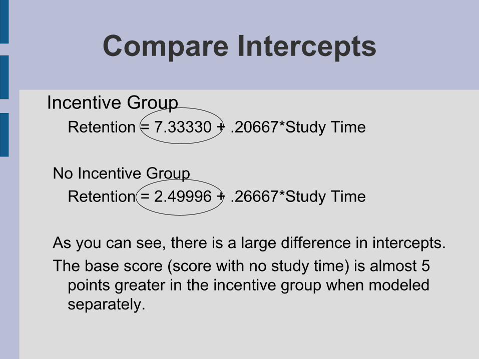
Compare Intercepts
Incentive GroupRetention = 7.33330 + .20667*Study Time
No Incentive GroupRetention = 2.49996 + .26667*Study Time
As you can see, there is a large difference in intercepts. The base score (score with no study time) is almost 5
points greater in the incentive group when modeled separately.

Compare Using Statistical Tests
● We cannot detect differences simply using the eyeball method.
● Even these guys need statistics.

Comparison● To set up a comparison, we first need to calculate
the regression equation using the full model (both variables together).
● The model will have both main effects (Incentive Group and Study Time) and well as the interaction between the two groups.
● Incentive is coded as 1 for No Incentive and -1 for Incentive
● …and SPSS spits out this:

Full Model● Retention = 4.916667
+ 2.36667*Study Time -2.416667*Incentive Group + .030000*(Study Time*Incentive Group)
– Also, don’t forget our separated models (using split file procedure in SPSS)
● Incentive GroupRetention = 7.33330 + .20667*Study Time
● No Incentive GroupRetention = 2.49996 + .26667*Study Time

Output of interaction term● bStudy Time*Incentive Group=.03000● t = 0.672● Sig(t) = 0.5093
– The interaction between Study Time and Incentive Group is Not Significant
– This indicates the difference between the coefficients for the regression of Retention on Study Time is not statistically significant for the two experimental groups (Incentive Group and No Incentive Group)

• Retention = 4.916667 + 2.36667*Study Time -2.416667*Incentive Group + .030000*(Study Time*Incentive Group)
• Incentive GroupRetention = 7.33330 + .20667*Study Time
• No Incentive GroupRetention = 2.49996 + .26667*Study Time
– Compute the slope of the full model by the average of the separate model’s slopes
• (7.3330+2.49996)/2 = 4.916667
Note: Intercepts

• Retention = 4.916667 + 2.36667*Study Time -2.416667*Incentive Group + .030000*(Study Time*Incentive Group)
• Incentive GroupRetention = 7.33330 + .20667*Study Time
• No Incentive GroupRetention = 2.49996 + .26667*Study Time
– Take the intercept of the full model and add the b for the incentive group (multiplied by dummy coding). This will obtain the intercept for the No Incentive group
• (4.916667+(-2.416667)*1) = 2.5 ~ 2.49996
Note: Compute intercept for No Incentive Group
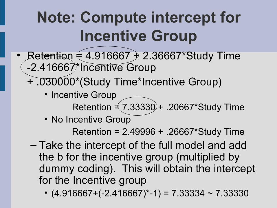
• Retention = 4.916667 + 2.36667*Study Time -2.416667*Incentive Group + .030000*(Study Time*Incentive Group)
• Incentive GroupRetention = 7.33330 + .20667*Study Time
• No Incentive GroupRetention = 2.49996 + .26667*Study Time
– Take the intercept of the full model and add the b for the incentive group (multiplied by dummy coding). This will obtain the intercept for the Incentive group
• (4.916667+(-2.416667)*-1) = 7.33334 ~ 7.33330
Note: Compute intercept for Incentive Group
• Retention = 4.916667 + 2.36667*Study Time -2.416667*Incentive Group + .030000*(Study Time*Incentive Group)
• Incentive GroupRetention = 7.33330 + .20667*Study Time
• No Incentive GroupRetention = 2.49996 + .26667*Study Time
– Compute the slope of Study Time for each Incentive Group. Take slope of study time and add coefficient of interaction (multiplied by dummy coding)
• 2.36667 + (.03*1) = 2.6667 ~ 2.6667
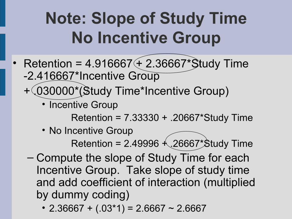
Note: Slope of Study TimeNo Incentive Group

• Retention = 4.916667 + 2.36667*Study Time -2.416667*Incentive Group + .030000*(Study Time*Incentive Group)
• Incentive GroupRetention = 7.33330 + .20667*Study Time
• No Incentive GroupRetention = 2.49996 + .26667*Study Time
– Compute the slope of Study Time for each Incentive Group. Take slope of study time and add coefficient of interaction (multiplied by dummy coding)
• 2.36667 + (.03*-1) = 2.0667 ~ 2.0667
Note: Slope of Study Time Incentive Group

Slope and Intercept Calculations
● All of the calculations on the previous slides can be done even when there are multiple categories for your variable.
● Instead of using 1 and -1, insert the appropriate dummy coding of the variables.

Overall Regression Equation● The author refers to the overall regression
model as the full model minus any interaction terms.
● This is a multiple regression of each independent variable individually on the dependent variable.
● …and SPSS give us:

Overall Regression Equation● Retention = 4.916667
+ .236667*Study Time – 2.041667*Incentive Group

Test of Significance of Slope of Study Time
● Slope of Study Time– bstudy time = .236667– t(N-k-1) = t(24-2-1) = t(21) = 5.3711 – sig(t) =.0000
● Significantly different from 0

Difference Between Intercepts● We already established that the b’s of Study
Time are not significantly different for the two Incentive Groups– The not significant interaction told us this
● Once this is established, it makes sense to determine if there are overall differences in terms of the experimental condition (i.e. Do subjects score higher overall in the Incentive Group)
● This can be tested by looking at significance of the b for the Incentive Group variables

Difference Between Intercepts● b for Incentive Group
– bIncentive Group = -2.041667– t(21) = -8.289– Sig(t) = 0.000
● This is significantly different from 0, indicating a difference in overall Retention between the two Incentive Groups– What is this difference?– (-2.041667*-1)-(-2.041667*1) = 4.08
● Subjects score on average 4 points higher in the Incentive Group when modeled together

Separate Regression Equations
● Instead of making completely independent models for the two groups, we can compute separate models for the two groups based on our Overall Regression Equation
● This way we can specify that the two equations have the same slope

Separate Regression Equations: Incentive Group
● Using Overall Regression Equation:– Retention = 4.916667 + .236667*Study Time
- 2.041667*Incentive Group● Equation is:
– Retention = 4.916667 + .236667*Study Time - 2.041667*(-1) = 6.958334 + 2.36667*Study Time

Separate Regression Equations: No Incentive Group
● Using Overall Regression Equation:– Retention = 4.916667 + .236667*Study Time
- 2.041667*Incentive Group● Equation is:
– Retention = 4.916667 + .236667*Study Time - 2.041667*(1) = 2.87500 + 2.36667*Study Time

Single Regression Equation● We can also represent the two groups in a
single regression equation by simply dropping the Incentive Group Variable:– Retention = 4.916667 + .236667*Study Time
● This model does not account for differences between the two incentive groups, which we found to exist
● Not a valid approach in this case, however, it may be appropriate in other examples

Separate Regression Equations: Incentive Group
● Using Overall Regression Equation:– Retention = 4.916667 + .236667*Study Time
- 2.041667*Incentive Group● Equation is:
– Retention = 4.916667 + .236667*Study Time - 2.041667*(-1) = 6.958334 + 2.36667*Study Time

Proportion of Variance Accounted For
● Here is the output given R2: Study Time R2 = .2434 Incentive Group R2 = .5795Interaction R2 = .0039
• The two variables in the model account for 82% of the variance present in the data
• We can test for significance of these using an F testStudy Time F=7.076 sig(F) = 0.014Incentive Group F = 68.712 sig(F) = 0.000Interaction F = 0.452 sig(F) = 0.509

Categorizing Continuous Variables
● Some researchers may find it beneficial to partition continuous variables into a number of categories
● In our example, even though Study Time was continuous, we could have also thought of it as a categorical variable with 4 levels (5, 10, 15, 20 minutes)
● A 2 X 4 ANOVA then can be computed

Categorizing Continuous Variables
● Another way of categorizing a continuous variable is often done in treatment-by-levels design.
● For example, a researcher may be interested in the difference between two teaching methods.
● Prior to beginning treatment, all subjects have a different intelligence level.
● The experimenter may want to “control” for intelligence in the design to piece out the information regarding the treatment
● The resulting ANOVA will portion out the variance related to the “control” variable

Categorizing Continuous Variables
● Some studies categorize continuous variables in an attempt to study possible interactions between the independent variables– Called Aptitude-Treatment Interaction (ATI), or
Attribute-Treatment Interaction (ATI), or Trait-Treatment Interaction (TTI)
● Different from previous categorization because the “control” variable is actually a factor of interest– In this same example, the researcher may want to
see if the treatments change the test scores differently for people with different intelligence

Categorizing Continuous Variables
● You can also categorize continuous variables in a counterproductive way
● This can occur if a researcher categorizes a continuous variable that has more than one attribute– For example, categorizing personality,
attitudes, ect.

Basis For Categorization● How do you categorize a categorical
variable?– Often, variables are cut in half at the median,
then labeled low or high● It should be noted that you should be
careful in your categorization, because not all “low’s” are created equal…
● What effect does categorization have?– Categorization leads to a loss of information
and a less sensitive analysis

The Study of Interaction● In the case where the is one continuous
variable and one categorical variable (as in our example in the beginning), the interaction answers the question of whether the regression lines of the dependent variable (Retention) on the continuous variable (Study Time) are parallel for all the categories of the categorical variable (Incentive Group)

Attribute-Treatment Interaction
● In our example, the Study Time was manipulated● In this research design, that is not the case (they may
simply ask how long the individual studied, for example)● The test of significance would be the same, however,
the interpretation of the interaction effect would differ● In the previous design, since we know Study Time was
manipulated, the cause for difference has to be related to the Incentive Group
● If we do not manipulate Study Time, the significance of the interaction may be a result of both the Incentive Group AND the Study Time

Types of Interaction Effects● There are two main types of interaction effects
– Ordinal Interaction● reflects the fact that an independent variable seems to have
more of an effect under one level of a second independent variable than under another level. If you graph an ordinal interaction, the lines will not be parallel, but they will not cross.
– Disordinal Interaction● when an independent variable has one kind of effect in the
presence of one level of a second independent variable, but a different kind of effect in the presence of a different level of the second independent variable. Called a crossover interaction because the lines in a graph will cross

Ordinal Interaction●

Disordinal Interaction●

Determining the Point of Intersection of Two Regression Lines
● Given the following two regression lines:y’a = 7 + .3Xy’b = 2 + .8X
• Point of Intersection (x) = (a1 – a2)/(b2 – b1)= (7-2)/(.8-.3) = 10
• Plug this x value into your equation(s) to get the y coordinate y=7+.3(10) = 10
• Coordinate of intersection is (10,10)

Comparing Regression Equations in Nonexperimental
Research● Nonexperimental designs are those in
which neither the categorical variable nor the continuous variable are manipulated
● The analytic approach in such designs is identical to that of experimental designs, however, it is the interpretation that differs
● The interpretation is often more complex and ambiguous in terms of the findings

The Study of Bias● One definition of test bias (Cleary, 1968)
– A test is biased for members of one subgroup of the population if, in the prediction of the criterion for which the test was designed, consistent nonzero errors of prediction are made for members of the subgroup. In other words, the test is biased if the criterion score predicted from the common regression line is consistently too high or too low for members of the subgroup
● This is the regression model for test bias● This idea of test bias occurs when there is an
interaction present when modeling two regression lines representing two categorical groups
Final Thought● Combining continuous and categorical
variables expand the practicality of regression analyses.
● The use of regression methods was highlighted in today's class.
● Next time we will cover the use of GLM...which Pedhazur calls ANCOVA (although we did ANCOVA today, too).