continued - institute and faculty of actuaries · i should also like to welcome peter savill to the...
TRANSCRIPT

continued Mortality I igation Reports
Number 12
Institute of Actwaries Faculty of Actuaries
Published by the Institute of Actuaries and tbe Fadty of Actuaries
1991

THE EXECUTIVE COMMITTEE OF THE CONTINUOUS MORTALITY INVESTIGATION
BUREAU
as on 30th June 1991
hrrritute Representatives FacuIty Representatives A. NeiU (Prmdent) C. Berman D. 0. Forfar C. G. Kirkwood (Deputy Chairman) I. C. Lumsde" J. I. McCutcbeon
THE IMPAIRID LIVE3 SUB-COMWTTQ
T. S. Le@ (Chairmaa) H.A.RLbmet S. F. Margutti C. G. Kirlnvood P. J. SpviU
A. D. WlUdc
THE PEmwaNT IIBUm INSURANCE S U B - c o r n
R H. Ptpmb (chairman) P. H. B a y k G. J. Hockinps R. I. L. Blackwood A. E. I. Jefnisr R. OankD A. R lclnnhaU E A. Hertznmn G. C. Orrrm
H. R. Watm

INTRODUCTION
THE Executive Committee of the Continuous Mortality Investigation Bureau of the Institute of Actuaries and the Faculty of Actuaries has pleasure in presenting this, the twelfth number of its Reports. This number contains what can hardly be described as a paper. but rather a book, consisting of several 'Chapters', described as 'Parts', some of which are attributed to named authors.
The paper--or book-is entitled 'The Analysis of Permanent Health Insur- ance Data'. and it describes the resultsof many years study by themembers of the PHI Sub-Committee. In it a radical new approach to the analysis of PHI data is presented, and it will be seen that it reconciles the tw-o previous approaches, the 'Manchester Unity' sickness rates method and the 'American' incidence rate and disability annuity method, which were previously thought to conflict.
Credit is due to the members of the PHI Sub-Committee for preparing this massive work, and in particular to Philip Bayliss and Howard Waters, whose names appear on the Parts for which they are particularly responsihle. Thanks are also due to the staff of Pensions and Insurance Computing Services, who provide the basic computing for the investigation. and also to the offices who have contributed PHI data over many years. receiving more promises of results than production of them. The Committee hopes that theoffices will feel that their forbearance is rewarded, though it isappreciated that the new method will not be understood without some effort.
I should also like to take the opportunity to pay tribute to the work of Hugh Jarvis. who resigned from the Executive Committee on his retirement in April. He had served on the Committee since 1980; latterly being Chairman of the Impaired Lives Sub-Committee. His place on the main Committee and as Chairman of that Sub-Committee is taken by Spencer Leigh.
I should also like to welcome Peter Savill to the Impaired Lives Sub- Committee and Roger Blackwood and Graham Hockings to the PHI Sub- Committee, to which they have recently been appointed.
June, 1991 A. D. Wilkie Chairman. Executive Committee

CONTENTS
... ... Introduction . . . . . . ... ... ... ... ...
... ... ... ... ... ... ... Contents ... ...
... ... ... ... ... ... ... List of Figures ...
... ... ... ... ... ... ... List of Tables ...
... ... The Analysis of Permanent Health Insurance Data ...
... ... Introduction . . . . . . ... ... ... ... ...
Part A: A Multiple State Model for Permanent Health Insurance by ... ... H . R . Waters ... ... ... ... ... ... ... ... ... ... ... ... ... Summary ... ... ... 1 Introduction ... ... ... ... ... ... ... ... ... ... ... ... ... 2 The Model ... ... ... 3 Parameter Estimation ... ... ... ... ... ... ... 4 Practical Difficulties of Parameter Estimation ...
... ... ... 5 Formulae for Probabilities ... ... ...
Appendix A-Parameter Estimation and Duplicate Policies ... ...
Part B: The Graduation of Claim Recovery and Mortality Tntensities by P . H . Bayliss ... ... ... ... ... ... ...
... ... ... Summary ... ... ... ... ... ...
... ... 1 Introduction ... ... ... ... ... ...
... 2 Preliminary Considerations ... ... ... ... ...
... ... 3 Recovery lntensities-Investigation ... ... ...
... ... 4 Recovery lntensities-Graduation ... ... ... ... ... 5 Mortality Intensities-Investigation . . . . . . ...
... ... 6 Mortality Intensities4raduation ... ... ... 7 Disability Annuities-Continuation Tables . . . . . . ... ...
V
(iii)
V
ix
xi

Part C: The Graduation of Sickness Inceptiopn Intensities by ... ... ... ... H . R . Waters ...
... ... Summary ... ... ... ... ... ... ... ... 1 The Statistical Model ... ... ... ...
2 The Available Data ... ... ... ... ... ... ... ... 3 The Number of Claim Inceptions ... ... ... ... 4 The Calculation of the Exposure ... ... ... ... 5 The Graduation Process ... ... ...
6 Results of the Przliminary Graduations ... ... ...
. . . . . . ... ... 7 Further Investigations ... ... ... 8 The Re-graduation of 0, for Deferred Period 4 Weeks
9 Conclusions and Further Comments . . . . . . ... ...
Part D: Computational Procedures for the Model by H . R . Waters
Summary ... ... 1 Introduction ... ... ... ... ...
... ... 2 Numerical Calculation of Probabilities ... ... ... 3 The Calculation of p, ... ... ... ...
4 The Constructiotl of an Increment-Decrement Table ...
... ... 5 Claim Inception Rates . . . . . . ... ... ... ... 6 Manchester-Unity-type Sickness Rates ...
7 The Exact Calculation of Monetary Functions ... ... ... ... Appendix Dl-Derivation of Formula (9) ...
Appendix D2-Demonstration that Formula (69)=(71)+(72) ...
... ... Part E: Calculation of Probabilities ... ...
... ... Summary ... ... ... ... ... ...
... ... 1 Mortality of the Healthy ... ... ...
... ... ... 2 Graphical Representation ... ... ... ... ... ... ... 3 Basic Probabilities ...
... ... ... 4 Aggregate Mortality Rates ... ...

Contents
5 Claim Inception Rates . . . . . . ... ...
... 6 Manchester-Unity Type Sickness Rates
7 Construction of Select Tables-Mortality Rates
8 Construction of Select Tables-Inception Rates
9 Construction of Select Tables-Sickness Rates
l0 Probabilities of Survival While Sick . . . . . . l l Deferred Periods 4. 13. and 26 Weeks . . . . . .
... Part F: Calculation of Monetary Functions
Summary ... ... ... ... ... ... 1 Annuities Payable in a Given Status: Total Sickness Annuities
... 2 Approximate Calculation of Annuities Using Functions
vii
... 104
... 107
... 108
... 110
... 115
... 119
... 120
... 227
... 227
... 227
... 232
3 Approximate Calculation of Annuity Values Using Manchester- Unity-Style Sickness Rates ... ... ... ... ... ...
4 Approximate Calculation of Annuity Rates Using Select Tables of ... ... Manchester-Unity-Style Sickness Rates ... ...
... 5 Values of Current Claim Annuities ... ... ... ... 6 Approximate Calculation of Annuity Values Using Inception Rates
and Current Claim Annuities . . . . . . ... ... ... ... 7 Approximate Calculation of Annuity Values Using Select Tables of
... ... ... ... Inception Rates . . . . . . ... ... 8 Premiums ... ... ... ... ... ... ... ... 9 Comparison of Sickness Rate and Inception Rate Methods ...
... ... ... ... ... ... ... References ... ... ... ... ... ... ... Glossary of Notation ... ...

LIST OF FIGURES
AI A diagrammatic representation of the model for sickness . . .
B1 Recovery rates: duration related factors: deferred periods separate
B2 Recovery rates: duration related factors: all deferred periods combined except for run-in periods .. . . . . . . . ... . . ,
B3 Recovery rates: duration related factors: extended to sickness durations greater than 1 year: all deferred periods combined excluding run-in periods . . . . . . , . , . . . . . . . . .
B4 Recovery rates: age related factors: deferred periods separate
B5 Recovery rates: age related factors: all deferred periods combined
B6 Mortality rates: duration related factors: all deferred periods combined ... . . . . . . . . . . . . ... . . . . . .
B7 Mortality rates: age related factors: all deferred periods combined
C1 Sickness inception intensities: deferred period 1 week ... . . . C2 Sickness inception intensities: deferred period 4 weeks ... . . .
C3 Sickness inception intensities: deferred period 13 weeks . . . . . .
C4 Sickness inception intensities: deferred period 26 weeks . . . . . .
E l Model of sickness . . . . . . . . . . . . ... . . . . . .
E2 Claim inceptions ... . . . , . . . . . . . . . . . ...
E3 Inception rates of type (a) for attained age 64 ... ... . . .
E4 Sickness rates for attained age 64 ... ... . . . ... . . .
F1 Calculating sickness benefit using sickness rates
F2 Calculating sickness benefit using inception rates of type (a) ... F3 Calculating sickness benefit using inception rates of type (b) ...
F4 Calculating sickness benefit using inception rates of either type ...

LIST OF TABLES
Graduated values of p,,:, ... . . . . . . . . . . . . . . .
Graduated values of 10,000 v,,,, ... . . . . . . . . . . . .
Graduated values of 10,000 v,,,, for durations over 5 years ...
Exposed to risk and comparison of actual recoveries with those expected according to the graduated rates . .. . . . . . . . . .
Exposed to risk and comparison of actual deaths with those expected according to the graduated rates for all deferred periods combined ... . . . . . . ... . . . . . . . . . . . .
Graduated double decrement tables of claim terminations . . .
Values of IR and IN used in the preliminary graduations of a.y ...
Values of 100,000 p ( y ; y ~ ) . . . .,. . . . . . . . . . .,.
Exposures (in years) at age x . . . . . . . . . . . . ...
Parameter estimates for the preliminary graduation ... ...
Preliminary graduation of U, for deferred period 1 week: estimated and graduated values of a, and actual and expected numbers of claim inceptions . . . . . . ... ... . . . . . . . . .
Preliminary graduation of U, for deferred period 4 weeks: estimated and graduated values of a, and actual and expected numbers of claim inceptions . . . ... ... . . . ... . . . . . .
Preliminary graduation of ax for deferred period 13 weeks: esti- mated and graduated values of a, and actual and expected numbers of claim inceptions .. . . . . . . . , . . ... . . . ...
Preliminary graduation of a, for deferred period 26 weeks: esti- mated and graduated values of a, and actual and expected numbers of claim inceptions . . . ... . . . . . . ... . . . . . .
Tests of the graduations . . . . . . . . . . . . ... . . .
The effect of eliminating terminations within 4 weeks of the end of the deferred period . . . ... ... . . . ... . . . . . . Reported and non-reported claim inceptions for deferred period 4 weeks . . . . .. . . . . . . ... . . . . . . . . . . . .
Parameter estimates and standard errors for the re-graduation of U, - for deferred period 4 weeks . . . . . . ... . . . ... . . .

xii
C13
C14
List of Tables
Tests of the re-graduation of U, for deferred period 4 weeks
Re-graduation of U , for deferred period 4 weeks: estimated and graduated values of U, and actual and expected numbers of claim inceptions ... ... ... ... ... ... ... ...
The effect of eliminating terminations within 4 weeks of the end of the deferred period . . . . . . ... ... ... ... ...
Graduated values of aJ
Graduated values of 10,OOOa,r.rr,,,,
Testing the data for deferred periods I week and 13 weeks against . . . . . . the graduated values of U, for deferred period 4 weeks
Testing the data for deferred periods 4 weeks and 26 weeks against . . . . . . the graduated values of U , for deferred period 13 weeks
Comparison of overall mortality rates ... . . , ... ...
Claim inception rates of type (a) per 10,000 ... ... ... Comparison of sickness rates: Table E19 and TableH1 of C.M.I.R. 7
Ratio of qsa for entry age shown to qM for entry age 16 . . . . . .
Ratio of q4 for entry age shown to q4,, for entry age 16 . . . . . .
Inception rates of type (a) for attained age 64 as percentage of those for age 16 at entry ... ... ... ... ... ... ...
Inception rates of type (a ) for attained age 64 as percentage of those for duration 5 . . . . . . ... ... ... ... ... ...
Maximum error in total claims
Sickness rates for attained age 64 as percentage of those for age 16 at entry . . . . . . . . , ... . , . ... ... ... ,..
Sickness rates for attained age 64 as percentage of those for dura- tion5 . . . . . . ... ... ... ... ... ... ...
E9
E10
E l l
E12
Maximum error in total weeks of sickness . . . . . . ... ...
Probabilities by age 65 conditional on being healthy at age 30 ... Aggregate mortality mL(x) conditional on being healthy at age 30
Claim inception rates of type (a) per 10,000 conditional on being healthy at age 30 ... ... ... ... ... ... ... Comparison of sickness rates: 4 weeks basis and Table H2 of
... ... C.M.I.R. 7 ... , . , ... .,. ... . , .

. . . List of Tables XIII
E13b Comparison of sickness rates: 13 weeks basis and Table H3 of C.M.I.R. 7 ... . . . . . . ... .., . . . . . . ... 124
E13c Comparison of sickness rates: 26 weeks basis and Table H4 of C.M.I.R. 7 ... . . . . . . . . . . . . . . . . . . ... 124
Tables E14 to E19 are on the 1 week deferred period basis, conditional on starting at age 30 with initial status healthy.
E14 Survivors (I) and transitions (d) at each age based on a radix of 1 .OOO,OOO . . . ... ... ... . . . ... ... ... 126
E15 Subdivision of sick in each given sickness period at each age ... 128
E16 rates: 52 X proportions sick among the living at each age for each sickness period . . . . . . . . . . . . . . . ... ... 130
E17 Decrement rates and life table . .. . . . . . . . . . ... 132
E18a Claim inception rates of type (a) per 10,000 living at given deferred periods at each age . .. . . . . . . ... . . . . . . ... 133
El8b Claim inception rates of type (b) per 10,000 living at given deferred periods at each age ... ... . . . ... ... . . . ... 134
E19 Sickness rates for each sickness period at each age ... ... 135
Tables E20a to E25 are on the 1 week deferred period basis.
E20a Select table of qrXl+, with 2 years selection ... ...
E20b Select table of q,.l+< with 5 years selection
E21a Select table of l rX l+ , with 2 years selection ... ... . . . . . . E21b Select table of with 5 years selection
E22a Select table of iatI+, with 5 years selection: methods A and B: deferred period ( d ) 0 weeks . . . . . . . . . . . . . . . . . .
E22b Select table of ia&,+, with 5 years selection: methods A and B: deferred period i d ) 1 week . . . . . . . . . . . . , . . ...
E22c Select table of jagl+, with 5 years selection: methods A and B: deferred period ( d ) 4 weeks .. . . . . ... . . . ... ...
E22d Select table of ia(il+, with 5 years selection: methods A and B: deferred period i d ) 13 weeks ... . . . . . . . . . . . .
E22e Select table of jagl+, with 5 years selection: methods A and B: deferred period ( d ) 26 weeks . . . . . . . . . . . . . . .

xiv List of Tables
E22f Select table of ia&]+, with 5 years selection: methods A and B: deferred period (d) 52 weeks . . . ... . . . . . . . . .
E22g Select table of in&]+, with 5 years selection: methods A and B: deferred period (d) 104 weeks . . . . . . . . , . . . . . .
E23a Select table of with 5 years selection: methods A and B: sickness period (ajb) 011 weeks ... . . . ... ... . . .
E23b Select tahle of if$+, with 5 years selection: methods A and B: sickness period (alb) l13 weeks . . . . . . ... . . . . . .
E23c Select tahle of @p+, with 5 years selection: methods A and B: sickness period (ajb) 419 weeks . . . . . . ... . . . . . .
E23d Select tahle of z@p+, with 5 years selection: methods A and B: sickness period (alb) 1311 3 weeks . . . . . . ... . . . . . .
E23e Select tahle of ;@P+, with 5 years selection: methods A and B: sickness period (alb) 26/26 weeks . . . .. . ... . . . . . .
E23f Select tahle of zf$+, with 5 years selection: methods A and B: sickness period (alb) 52/52 weeks ... .. . . . . . . . . . .
E24 Sickness rates i(x, l 04/all,x-xo) . . . . . . . . . ... . . .
E25 Average probabilities,pi(x,d), of survival while sick from duration 0 to duration d, sickness commencing between ages X and X + 1, using values conditional on entry at age 16 ... . . . ... ...
Tables E26 to E29 are on the 4 week deferred period basis
E26 Select table of q,,,,, with 5 years selection . .. . . . . . . . . .
E27 Select table of ia&,+, with 5 years selection: methods A and B: deferred period (d) weeks . . . , . . . . . . . . ... ...
E28a Select table of ~ f $ + ~ with 5 years selection: methods A and B: sickness period (alb) 4/9 weeks . . . . . . ... . . . ...
E28b Select table of z@+, with 5 years selection: methods A and B: sickness period (alb) 13/13 weeks ... ... . , . . . . ...
E28c Select table of ~ f $ + ~ with 5 years selection: methods A and B: sickness period (a/b) 26/26 weeks . . . . . . . . . . . . ...
E28d Select table of -g!+, with 5 years selection: methods A and B: sickness period (aib) 52/52 weeks . . . . . . . . . . . . . . .
E29 Sickness rates z(x, l04/all,x-xo) . . . ... . . . . . . . . .

List of Tables xv
Tables E30 to E33 are on the 13 week deferred period basis,
E30 Select table of q,,~+, with 5 years selection .. . . . . . . . ... 196
E31 Select table of ia(',I+, with 5 years selection: methods A and B: deferred period (d) 13 weeks . . . ... , . . . . . ... 198
E32a Select table of z@f+, with 5 years selection: methods A and B: sickness period (alb) 13/13 weeks ... ... ... ... . . . 200
E32b Select table of z&+, with 5 years selection: methods A and B: sickness period (alb) 26/26 weeks . . . . . . . . . ... .. . 202
E32c Select table of &p+, with 5 years selection: methods A and B: sickness period (alb) 52/52 weeks . . . . . . ... ... ... 204
E33 Sickness rates z(x, l04/all,x- xo). . . . ... ... ... . .. 206
Tables E34 to E37 are on the 26 week deferred period basis.
E34 Select table of qlXl+, with 5 years selection .. . . . . . . . ... 212
E35a Select table of in(',]+, with 5 years selection: methods A and B: deferred period (d) 26 weeks ... ... ... . . . ... 214
E35b Select table of i d l + , with 5 years selection: methods A and B: deferred period (d) 52 weeks ... ... ... ... ... 216
E36a Select table of zfip+, with 5 years selection: methods A and B: sickness period (a/b) 26/26 weeks ... ... ... ... ... 218
E36b Select table of z@f+, with 5 years selection: methods A and B: sickness period (a/b) 52/52 weeks ... ... ... ... . .. 220
E37 Sickness rates r(x,l04/all,x-xo) . . . . . . . . . . . . ... 222
Tables F1 and F2 are on the l-week deferred period basis, conditional on starting at age 30 with initial status healthy: rate of interest 6%.
F1 Present values of annuities payable continuously in each status for each term from starting age . .. .. . ... ... . , . . . . 228
F2 Present values of annuities payable monthly in advance in each status ... ... . . . . . . ... ... ... . . . . . . 230
Tables F3 to F5 are on the l-week deferred period basis, rate of interest 6%.
F3 Present values of continuous current claim annuities of 1 per year ceasing a t age 65 . .. ... ... ... ... ... ... 238

xvi List of Tables
F4 Average values of continuous current claim annuities of 1 per year, payable while sick commencing at given age and given duration of sickness and ceasing at age 65: types (1) and (2) . . . . . . ... 244
F5 Annuity values and annual premium rates for a benefit of 1,000 per year with selected deferred periods for each term from starting age, conditional on starting at age 30 with initial status healthy: premiums payable 12 times per year in advance: benefits treated as payable continuously ... ... ... . . . . . , . . . .. . 248

CMIR 12 (1991) 1-263
THE ANALYSIS OF PERMANENT HEALTH INSURANCE DATA
INTRODUCTION
IT has always been envisaged by the PHI Sub-Committee, from the first Report of the Advisory Sub-Committee for the investigation of sickness statistics in September 1971 (reprinted in 'Investigation of Sickness Statistics', C.M.I.R. 2 (1976)), that an investigation on a 'Disability Annuity' basis would be carried out. However. it was noted in that first Report that "disability annuities have to be derived from 'select' data with a very long period of selection (15 years was used in the United States of America) and a number of years' experience must be amalgamated to produce results which are statistically reliable". Records for claims were therefore gathered in a form which would allow rates of termination ofclaim 'whether by recovery or death' to be investigated. In this Report the Suh- Committee presents the results of its investigations on these lines for the first time.
Rates of claim inception, i.e. 'rates of starting a claim at age X' have been calculated and published from the very first investigation. Graduations of the male claim inception rates for 1972-75 were published in 'Sickness Experience 1972-75 for Individual Policies', C.M.I.R. 4 (1979) and graduations of the male standard experience for 1975-78 were published in 'Sickness Experience 1975-78 for individual PHI Policies', C.M.I.R. 7 (1984).
In this Report the Sub-Committee is at last able to present its investigations of sickness claims on a 'disability annuity' basis for consideration by the actuarial profession and by PHI offices. The Report is long. and it has taken a long time to produce. As the investigation progressed it became apparent that a new and clearly stated model of sickness was required. Such a model had been proposed by Dr H. R. Waters (1984). In 1986 Dr Waters was invited to become a member of the Sub-Committee. His contribution to the development of the model is readily apparent from the fact that three of the six Parts into which this Report is divided carry his name as the author.
The use of this new multiple state model resulted in complexities that had not initially been suspected. I t was felt that the use of the full model. although theoretically justifiable, resulted in what were probably unacceptably heavy comvutational requirements. It was necessary therefore to search for a way of similifying the reshts in order to fa~ilitate~ra~ticalcalculations. This too took a substantial amount of time, as did the search for satisfactory bivariate formulae to represent rates of recovery and death which varied both by age and by duration of sickness. This latter task fell to Mr P. H. Bayliss, who had been responsible for the graduation work in the earlier reports on sickness statistics. Part B of this Report is recognised as his work.

2 Introduction
A major advantage of the multiple state model used as the basis of this Report is that it allows the two different approaches, the Manchester Unity Sickness Rate approach and the Claim Inception Rate and Disability Annuity approach, to be seen as alternative representations of the same underlying model, providing alternative ways of ca lcu~~t ing the same functions. The apparent conflict between the approachis is seen to be groundless, and it is shownin Part F of the Report that each aonroach has its merits for calculatinz the values of different tvnes of
L . < L
benefit. The choice is not one of principle, but of computational convenience. It has to be noted, however, that a single Sickness Rate table, as in the original Manchester Unity tables, does not provide a satisfactory approximation; rather a table dependent on age at entry is required.
In its Report in C.M.I.R. 7 (1984) the Sub-Committee discussed the problems of interpreting figures for sickness rates gathered on an 'aggregate' basis, i.e. not sub-divided by duration since the commencement of the policy. The investiga- tions in Part E about the construction of select tables of sickness rates demonstrates why an 'aggregate' rather than a 'select' investigation is unsatisfac- tory, at least for the sickness period denoted as 'l04!all'.
Many techniques new to the actuarial profession have had to be developed in the course of this investigation. These include:
graduation of bivariate data, and corresponding graduation tests; numerical solution of the simultaneous differential equations that define the multiple state model; criteria for condensing complete tables of rates, sub-divided by age at entry 2nd atlalnCJ age, into table5 uith a select period for a li~n~ted numbcrof !.cm: In\e\ t~gat lx Into thc rcl~tivr. accuraclcr of d~fferent methods oiapprox~ma- tion.
Many of these are interesting problems in their own right. The Report is sub-divided into six Parts. In Part A the mathematical basis of
the multiple state model is described. In Parts B and C the rates of recovery and death among the sick and rates of falling sick among the healthy are analysed, and graduation formulae that satisfactorily fit the data are developed. In Part D the numerical methods required to solve the differential equations of the model are described, ready for Parts E and F, in which the calculation of probabilities and the calculation of monetary functions are described, and many numerical examples are given.
A glossary of the notation for those functions that appear in more than one Part is included as an Appendix.
It should he noted that the data used throughout this investigation is that for the Male Standard Experience for individual PHI policies for 1975-78. Comparison of the experiences for females, for group and unit cost policies and for all investigations for 1979-82 will follow in subsequent Reports.
The size of the task that has been undertaken by the members of the Sub- Committee and in particular by members of the Task Force responsible for the work-R. H. Plumb (Chairman), P. H. Bayliss, E. A. Hertzman, G . C . Orros,

Introduction 3
H. R. Waters and A. D. Wilki+has been daunting. The length of this Report may be just as daunting to many readers. The Task Force in particular feels perhaps that, to adapt Horace:
but it hopes that some others may attempt to scale the mountain with them. Those who feel that they need to revise their knowledge of the practical aspects
of PHI business may like to read or reread the papers by Bond (1963), Sansom (1978) and Sanders and Silby (1988). Those who wish to review the earlier investigations of the PHI Sub-Committee are referred in particular to reports in C.M.I.R. 2 (1976), C.M.I.R. 4 (1979) and C.M.I.R. 7 (1984).

PART A: A MULTIPLE STATE MODEL FOR PERMANENT HEALTH INSURANCE
SUMMARY
The mathematical model for PHI which has been investigated by the C.M.I. Bureau, and which is the subject of this Report, is introduced in this Part. This Part also provides a brief and somewhat general introduction to topics which will be discussed more fully in other Parts of this Report; in particular, parameter estimation is discussed in sections 3 and 4 of this Part, and in much more detail in Parts B and C. In section 5 of this Part we discuss the derivation of formulae for probabilities; the numerical evaluation of these probabilities is discussed in detail in Part D.
1. I The purpose of this Part is to describe a mathematical model which can be used as a model for PHI business. This model can perform two functions:
(i) it can form the basis for the statistical analysis of PHI data and (ii) it can be used to derive formulae, for example in terms of claim inception
rates and disability annuities or Manchester Unity type sickness rates, which could conveniently be used for valuing and setting premiums for PHI business.
1.2 The need for a new model for PHI is apparent on reading the most recent report of the PHI Sub-Committee of the Continuous Mortality Investigation Bureau, Continuous Mortalih. Investigation Reports 7 (1984). subsequently referred to as C.M.I.R. 7. Part 4 of C.M.I.R. 7 is a detailed explanation of the reasons why Manchester Unity type functions are considered unsuitable for valuing and setting premiums for modern PHI business and throughout the report it is clear that the Sub-Committee have experienced difficulties as a result of estimating a quantity, which is very complicated mathematically, using estimates whose statistical properties are unknown.
1.3 The requirements of a model for PHI are stated below:
(i) It should be sufficiently realistic. Any model incorporates some simplifi- cations but these should not be so severe as to make it difficult to accept as
5

6 The Analysis of Permanent Health Insurance Data
a model for the purposes being considered. For example, a model for PHI which has recovery rates depending only on the policyholder's attained age and not on the duration of his sickness may be considered too unrealistic to be of any use.
(ii) It should be possible to use the data which is available, or which could easily be made available, to estimate the parameters which determine the model, and, more importantly, to estimate them in such a way that the statistical properties of the estimators are known.
(iii) It should be possible to derive from the model numerical values of some functions which can conveniently be used to set premium rates for, and carry out valuations of, PHI business.
Broadly speaking, this Part discusses (i) and (ii) above for the model being proposed; (iii) is discussed in Part D of this Report.
1.4 The model for PHI discussed in this Part is a multiple state model with three states, Healthy, Sick and Dead. It is very similar to a standard illnessjdeath model which first appeared in the actuarial literature early in this century, see Du Pasquier (1912, 1913), and which was used for illustrative purposes by Waters (1984) in a general discussion of multiple state models. The essential difference between the earlier model and the one discussed in this Part is that. whereas in the earlier model all probabilities depended only on the policyholder's attained age, in the proposed model, although all probabilities still depend on the policy- holder's attained age, the probabilities bf either recovering & dying froma state of sickness denend also on the duration of the sickness. The model is described in ~ ~~
detail in 52 of this Part. Hoem (1972) discusses some mathematical aspects of models of this type and indicates that it was proposed as long ago as 1924 as a model for health insurance.
1.5 The important quantities for the proposed model are the transition intensities, which are analogous to the force of mortality for a life table, and in 93 we discuss how these could be estimated in such a way that the statistical properties of the estimators are known, at least asymptotically.
The discussion in 93 assumes there are no problems caused by having incomplete data. In practice this is not the case and in 54 we discuss the practical ~rohlems of Darameter estimation resultine from usine onlv that data which is currently available to the PHI offices and ience to the-C.M.I. Bureau
1.6 In-@ we show how, given the transition intensities, wecan derive formulae for some of the important probabilities for the model. Some of these probabilities can be easily evaluated but in some cases the resulting formulae are integro- differential equations. The numerical solution of these equations will be discussed in Part D of this Report.
2 . THE MODEL
2.1 The model proposed as a basis for the analysis of PHI data can be very simply described, in intuitive terms, with the help of Figure Al. On effecting his

Part A: A Multiple Slute Model for P.H.I. 7
policy the policyholder enters state H (since we assume he is not sick at that time). From state H he may transfer at any future time either to state S, i.e. become sick. or to state D. i.e. die. mo te that entering state S is not eauivalent to making a claim since to make a claim the policyholdLr must remain in state S for at least the deferred period of his policy.) The transition intensities, or forces of decrement, for these two transitions are denoted crx and p, respectively and depend only on X, the policyholder's attained age. Once in state S the policyholder may transfer back to state H, i.e. recover, or transfer to state D, i.e. die. The transition intensities for these transitions are denoted p,, and v,,~ respecti\ely and depend on r , he policyholder's atramcd age, and z . thu d~ ra t i on of h15 current s~ckness. Note that all thc probabilities in this model depend only on the policyholder's attained age and, in some cases, on the duration of his current sickness. These probabilities take no account of any other information; for example, they do not take account of the number of, or durations of, or time since, any previous periods of sickness.
Dead D 'D' Figure Al . A diagrammatic representation of the model for sickness.
Sick S Heolthy H
2.2 The model can be described more formally in terms of a pair of continuous time stochastic processes
i Y(X), Z(x)l X > 0 (1)
Y(x) can take any of the three values H, S or D and we interpret the event
{ W ) = HI,
for example, to mean 'the policyholder is healthy at age X'.
p x.2
'=X . fl . .

8 The Ana1ysi.v of Permanent Healfh Insurance Data
Z ( s ) takes values in [O,m] and is defined as follows Z(x) = maxjt : r G x and Y(x-11) = Y(x) for all h such that 0 < h G r) so that Z(x) denotes the duration, for a life now age X, of the sojourn so far in the current state, Y(x). Hence the event
{Y(x) = S, Z(X) = z) is the event that the policyholder is sick at age x and that the duration of his current sickness is z .
2.3 The joint process (1) is assumed to be a Markov process so that the future of the process after age x depends only on the values of Y(x) and Z(s) and not on any other eventsprior to age X. This means that, for example, if the policyholder hasjust fallen sick, the probability that he will remain sick for a long period takes no account of information such as that he has experienced many lengthy or short periods of sickness in the past.
2.4 We shall use the following notation
,pi,k = P [Y(x+ t ) = kl Y(x) = j and Z(x) = zl
whe1ej.k = H,Sor D and t.x,z 2 0. (Note that all the probabilities relating to the model are conditional on some information: unconditional roba abilities have no meaning in this model.) We assume that 'if the current state is H, i.e. if the policyholder is healthy at agex, then the futureof the process does not depend on the duration of the current period in F t te H i.e. how long the policyholder has
HJ HD been healthy. Formally, we assume ,p, .: . ,p,: and , p , : are all independent of the HH HS m value of z and so we shall denote these probabilities , p , , ,p , and ,p,
respectively. We also assume, for obvious reasons,
that Dk ,p , . ;=O k = H o r S
and ,p:? = 1 The following notational definitions will be useful later in this Report:
HH , P , = P[Y(x + f) = Hand Z(x + 1) 2 t 1 Y(x) = H ] (2)
- ,P: = P[Y(x + 1) = S and Z(x + t) = I + 11 Y(\-) = S
and Z(x) = z] (3)
E SS In the special case where z = 0, we shall denote ,p,,o by ,p, Note that the probability of staying healthy from age x to agejx + I),
H given that the individual was healthy at age X. (This is not the same as ,p , .)Note also that ,p<% the probability of stayingsick from agex to age(x + t), given that at age x the individual was sick with duration of sickness z .
We shall assume that all probabilities for our model are mathematically well behaved, in particular continuous, functions of n , t, x and z.

Part A: A Multiple State Modelfor P.H.I. 9
2.5 The transition intensities between the three states are denoted p,, U,, v , , ~ and p,,; and are defined as follows
p, = Lim,pyjr I - " -
(5)
We shall assume that all the above limits exist and that the transition intensities are mathematically well behaved functions; in particular we assume
all the transition intensities are continuous functions of either s or (X,;). (9)
An important consequence of (9) is that
the transition intensities are bounded on any bounded set of values of (x,z). (10)
Using (9) and (10) it can be shown that for any time interval (r,t + t)
P[2 or more transitions in (f,t + T)] = o(z) (11)
P [ Y ( x + f + r ) = S Y ( x + f ) = H ] = r . u , + , + o ( r ) (12)
P [ Y ( x + t + r ) = D I Y ( x + t ) = H ] = r ~ p , + , + o ( r ) (13)
P [ Y ( x + r + z ) = H I Y ( x + t ) = S a n d Z ( x + t ) = ~ ] = r . p , ~ + , , ~ + o ( r ) (14)
P [ Y ( x + t + r ) = D j Y ( x + t ) = S a n d Z ( x + t ) = z ] = ~ ~ v , , , ~ + o ( t ) (15)
where O(T) is any quantity such that
3. PARAMETER ESTIMATION
3.1 To be able to use the model described in the previous section we need to be able to estimate some parameters which determine the model. The choice of the parameters to be estimated depends on the form of the data available, but, in general, the most obvious choice for our model is the set of transition intensities. The reasons for this are discussed in Waters (1984) and in more detail in Hoem and Funck Jensen (1982).
10 The Analysis of Permanent Health Insurance Data
3.1 There IS well c.~ahlishr.d .;tat~stl~.al theory soncernlng the uttlm.~tion of mmsltlon inten.;ltles: u d u l rcl'ercnccz are S\erilrun I 1965,. Hocm I 1969. 19761. Aalen and Hoem (1978) and Borgan (1984). In this sectionwe shalfdisc&s how we could estimate the transition intensities given data in the most convenient form. We shall not discuss the theory underlying the estimation procedure; the reader interested in a more detailed treatment should consult the references given above. In the next section we shall discuss the oractical oroblems resultine from having available only that data which is curreniy avai~ad~e to the C.M.I. &eau.
3.3 Suppose we can observe over a period of time a group of PHI policies as they move between the states of our model as described in g(2.1). We shall, in this section, assume
(a) the behaviour of any single policy is independent of the behaviour of the other policies and
(b) we can observe every transition made by a policy.
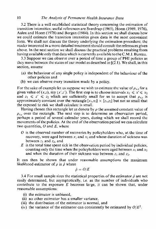
For the sake of example let us suppose we wish to estimate the value of p,, for a given value of ( v ) , say (X'$). The first step is to choose intervals x, G X'< x2 and 21 G z' G 22 which are sufficiently small for us to accept that p , , is approximately constant over the rectangle [xl,x2] X [zl,z2] but not so small that the exposed to risk we shall calculate is small.
Having chosen this rectangle let us denote by p the assumed constant value of p , ; over the rectangle. The next step is to determine an observation period, perhaps a period of several calendar years, during which we shall record the movements of the policies. At the end of the observation period we can calculate two quantities, 0 and E, where
0 is the observed number of recoveries by policyholders who, at the time of recovery, were aged between X, and x2 and whose duration of sickness was between zl and i2, and
E is the total time spent sick in the observation period by individual policies, counting only the time when the policyholders were aged between x, and x2 and when the duration of their sickness was between z , and z2.
It can then be shown that under reasonable assumptions the maximum likelihood estimator of p is (i where
6 = OIE
3.4 For small sample sizes the statistical properties of the estimator (i are not easily determined, but asymptotically, i.e. as the number of individuals who contribute to the exposure E becomes large, it can be shown that, under reasonable assumptions:
(i) the estimator is unbiased, (ii) no other estimator has a smaller variance, (iii) the distribution of the estimator is normal, and (iv) the variance of the estimator can consistently be estimated by 0/E2.

Part A: A Multiple Stute Model for P.H.I. 11
Speaking very loosely we can assume for large sample sizes that
f i - N ( P . O ~ E ~ )
Investigations by Schou and Vaeth (1980) suggest this distributional assumption is reasonable if the expected number of recoveries exceeds 10.
3.5 By dividing the range of values of (x,z) into a number of non-overlapping rectangles, assuming that p,: is approximately constant over each rectangle and estimating this constant value in the manner described above we can obtain a sequence of point estimates of p , , with known asymptotic statistical properties. The same procedure can be used to obtain sequences of estimators of a,, p, and v,, at selected points. It can be shown that each of the resulting estimators is independent of all the other estimators both for the same transition intensity and for the other three transition intensities.
3.6 With a set of point estimates ofp,,: (or g,, pA or v , , ) with known asymptotic distributions it would be possible to test for significant differences between recovery rates estimated from independent sets of data. There are some obvious questions of interest which could be investigated in this way:
(i) are recovery rates estimated from groups of policies with different deferred periods significantly different?
(ii) are recovery rates obtained from current data significantly different from those obtained from earlier data?
(iii) are recovery rates estimated from the experience of one group of offices significantly different from those estimated from the experience of another group of offices?
A simpleexample ofhypothesis testing in this way is given in Hoem and Funck Jensen (1982, $4.1).
4. PRACTICAL DIFFICULTIES OF PARAMETER ESTIMATION
4.1 In our discussion of parameter estimation in $3 we made two important assumptions, (a) and (b) in $(3.3), which are unlikely to hold in practice. In this section we shall discuss how in practical terms we could estimate the transition intensities using only that data which is currently available to theC.M.1. Bureau. In particular we shall discuss in turn problems due to:
(i) duplicate policies, (ii) observing transitions out of state Sonly when the duration of the sickness
is greater than the deferred period of the policy, (iii) observing transitions from state H to state Sonly when the duration of the
ensuing sickness is greater than the deferred period of the policy, (iv) not observing any transitions from state H to state D.
4.2 It is likely that any large group of PHI policies will contain some duplicates,

12 The Analysis of Permanent Health Insurance Data
i.e. several policies effected by the same life, and the presence of duplicates, for obviousreasons,makes assumption (a)in§(3,3)difficult tojustify. Let us suppose we wish to estimate p as described in sg(3.3) and (3.4) but the data contain duplicates. Let 0' and E be the observed numbers of transitions and the observed exposure without eliminating duplicates. We assume we know that a proportion f, of individuals contributing to E have exactly t policies and we denote by mi the I-th moment about zero of the distribution of policies: so that
m ,= E t ' . , / ; i = 1 .2 , . . . . ,=I
Under reasonable assumptions, it can be shown that if we define the estimator p'
by p' = O'!E'
then, loosely speaking,
p' - N(p.(O'IE'')(nl;n?,))
(The derivation of this is given in the Appendix.) Hence, the only result of not eliminating duplicates has been to increase the (asymptotic) variance of our estimator for p by a factor (m2/ml). This is precisely the 'correction factor' for duplicates to be found in C.M.I.R. 7 (1984. Appendix F), whose history can be traced back via Daw (1951) to Beard and Perks (1949). This is not surprising since the argument used in the Appendix to derive it is the same as that used by these earlier authors, although the present setting is somewhat different.
4.3 When calculating probabilities for our model, as we shall see in the next section, we shall need to know, amongst other things, the values of p,,? and VIZ for values of the duration of sickness : from zero upwards. Suppose we are considering a group of policies with deferred period d. It is very unlikely that we shall be able to observe transitions out of state S, either recoveries or deaths, if the duration of the sickness is less than d and hence we cannot use the method of 53 to estimate or v.,; for a value of i less than d. One possible way of reducing the scale of this problem would be to test whether. for example, recovery rates were significantly different for policies with different deferred periods. If they were not. it would be possible to estimate p,; for some values of z less than dby making use of data relating to policies with deferred periods less than d. Even if these recovery rates were significantly different. it might be reasonable to assume that p , , followed a similar pattern for policies with different deferred periods. A practical solution to the problem, whether we can reduce its scale or not, is to extrapolate from graduated values of p,., and v,.; for values of z for which we can estimate these parameters from data, to values of z for which we cannot.
4.4 The estimation of U, is likely to be more difficult than that of p , ; and v,,:. The problem is that in practice a sickness of less than the deferred period of the policy is unlikely to be reported and so i t is not possible to determine either the

Purr A: A Multiple Stulc Model for P.H.I. 1 3
relevant number of transitions or the exposure necessary to estimate a, as outlined in $3. Hence we are forced to adopt a somewhat different approach. Let us suppose we wish to atimate a, at a point X' for policies with deferred period d. Recall from$2 that dp:sdenotes the probability that a policyholder who falls sick at age X will remain sick for at least a period d. It will be shown in the next section that this probability is a function only of p,z and v,,, whose estimation is independent of that of a,. Now c h o o s e ~ n interval X , < x'<.x2 over which we may reasonably assume both a, and dp:Sto be approximately constant and let 0
and n respectively denote these assumed constant values. Intuitively, the product a,n is the intensity of falling sick and staying sick for at least a period d for policyholders aged between xl and s2. The population at risk, i.e. exposed to this intensity, is the set of policyholders who are in state H, i.e. who are not sick, and we must try to identify this population using only the data we assume to be available. Let N(t) denote the number of policyholders who, at time t , are aged between X, and x2 and whose policies have deferred period d. We have to subtract from this number those policyholders who are in state S a t time t , and we do this in two stages. Let Qi(t) denote the proportion of policyholders in N(t) who are sick at time 1 and whose sickness. at time I , has already lasted beyond the deferred period d and hence become a claim. Let Q2(r) denote the proportion of policyholders in N(t) who are sick at time t and whose sickness, at time l , has not yet lasted, and may or may not last. beyond the deferred period. Now define
so that M(t) represents the number of policyholders who, at time I, are aged between .X, and x2. are healthy and have policies with deferred period d . The appropriate exposure we wish to calculate is E. where
Tl and T: denote the start and the end of the observation period so that E represents the total time spent in state H during the observation period by policies with deferred period d. counting only that time when the policyholder is aged between X , and x2. Let us assume for the moment that we can calculate E from the available data and also that the data does not contain any duplicate policies; we shall return to these points in the next paragraph.
Let I denote the number of sicknesses among policies with deferred period d which start in the observation period, for which the policyholder is aged between xi and X? at the start of the sickness and whichlast beyond the deferred period. (I is equivalent to the number of claims which start in [T, + d , T 2 + d ] and for which the policyholder is aged between ( X , + d ) and (.x?+d) at the start of theclaim.) As a result of the way in which we assume data to be collected_ the exposure E is a random variable whose distribution depends on the parameter U. However. if we

14 The Analysis of Permanent Health Insurance Data
regard E as in some way pre-determined then I has a Poisson distribution with parameter o.7r.E. (See Sverdrup (1965, $8) for an interesting discussion of this point.) Even if we do not assume that E is pre-determined, it can be shown that, asymptotically and under some reasonable assumptions, I has a Poisson distribution with the parameter given above. (See Hoem (1987, Appendix 2) for details.)
Hence we may regard 6, where
6 = I/(z . E)
as a maximum likelihood estimator of o which, asymptotically, has a normal distribution whose variance can be consistently estimated by I/(n.E)'. For the purposes of hypothesis testing we may assume that
A - N(a, I/(n . E)') (17)
4.5 The estimation of a in the previous paragraph assumed that duplicate policies had been eliminated from the data. Let I and Edenote, as in the previous paragraph, the number of claims and the exposure, assuming duplicate policies have been eliminated and let P and E' be the corresponding quantities assuming duplicate policies have not been eliminated. Let mj denote, as in s(4.2). the i-th moment about zero of the distribution of policies per policyholder (for the relevant set of policyholders). Using the same argument as was used in §(4.2), we can show that we can estimate a by a', where
G' = I ' / (n . E ' )
and that corresponding to (171, we have
U' = N(u,(I'l(n . E')') (%/m,))
The major difficulty with the estimation procedure for ox described in this section is that, although we should be able to determine, or estimate. N(T).Q,(t) and I from the available data, it is unlikely, for obvious reasons, that we will be able to estimate Q2(t) directly. However, if we knew the vasl,,, of all the transition intensities, including a,, we could calculate &,.-,p, for various values of x ( < X ' ) , as we shall see in the next section, and from these values we could estimate Q2(t). Hence we could estimate a, using an iterative procedure as follows:
(i) start with a reasonable value for Q2(t) and estimate a as described in x4.41,
(ii) use theestimates from (i), and the values of the other transition intensities, HS to re-estimate Qz(t) by calculating d,,.-,p, , the probability that a life who
was healthy at some age x ( < X') is sick at age X' with duration of sickness less than d,
(K) use the new estimate of Q:(I) to re-estimate G,, (iv) continue this procedure until the estimates of Q'(t) and U, converge to
limiting values.

Purl A: A Multiple State Model for P.H.I. 15
4.6 The practical estimation of px is likely to be even more difficult than that of U, since we cannot reasonably expect to have any information about transitions direct from state H to state D. One solution to this problem would be to assume some arbitrary values for px; for example, p, equals the mortality of select assured lives at duration zero. Another solution could be to assume that policyholders who effect their policies at some conveniently early age will_ overall, experience the mortality of a known table, say A1967-70 Ultimate. The overall force ofmortality at any future age X' for this population can be expressed as a function of p,., and p,, a,, p , , and v , ; for X < X'. By equating this overall force of mortality to that of the known table, p,. could be calculated. This will be discussed further in 95 and also in Part D.
5. FORMULAE FOR PROBABILITIBS
5.1 In this section we shall indicate how we can derive formulae for some of the probabilities for our model. We shall assume throughout this section that the transition intensities are known functions of X or of (x,z). The formal derivations of formulae for all but the very simplest probabilities are extremely lengthy and for this reason we shall omit them. However, most of the formulae can be easily derived on an intuitive level and we shall give some of these intuitive derivations.
HH SS HH HS 5.2 The probabilities we shall discuss in this section are ,p, , ,p ,,Z, ,p, ,,,,p, , HD and , p , , which are all defined in 52. These probabilities satisfy the following
(integro-) differential equations:
= 0 for W > t
It should be noted that formulae (18) and (19) are just generalisations of the corresponding formula for ,p, in terms of the force of mortality for an ordinary life table. (See, for example, Neill(1977, formula (l .6.12)).) Note also that all the
16 The Analysis of Permanent Health Insurance Data
above formulae can be regarded as 'Kolmogorov forward equations' for our model. (See, for example, Cox and Miller (1965, 54.3.)
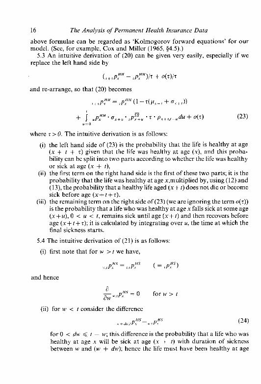
5.3 An intuitive derivation of (20) can be given very easily, especially if we replace the left hand side by
and re-arrange, so that (20) becomes
+ J "P:~.%+".,P~" . z . ~ ~ + i . l - " d u + O(T) U = "
(23)
where T > 0. The intuitive derivation is as follows:
(i) the left hand side of (23) is the probability that the life is healthy at age (X + t + z) given that the life was healthy a t age (X), and this proba- bility can be split into two parts according to whether the life was healthy or sick at age (X + 1);
(ii) the first term on the right hand side is the first of these two parts; it is the probability that the life was healthy at age x,multiplied by, using (12) and (13), the probability that a healthy life aged (.r+t) does not die or become sick before age (X+ t +z),
(iii) the remaining term on the right side of (23) (we are ignoring the term o(t)) is the probability that a life who was healthy at age X falls sick a t some age @+U), 0 < u i 1, remains sick until age (X+ 1) and then recovers before age (X+ t+r): it is calculated by integrating over u_ the time at which the final sickness starts.
5.4 The intuitive derivation of (21) is as follows:
(i) first note that for 1v > t we have,
H.5 ,,.,PP" = , ,P, ( = ,P!")
and hence
(ii) for W < t consider the difference
for 0 i dw t - W; this difference is the probability that a life who was healthy at age x will be sick at age (X + t) with duration of sickness between w and (M, + dw); hence the life must have been healthy at age

Part A: A Multiple Stare Model for P .H.I . 17
(X + t - w - dw), fallen sick between ages (X + t - n, - dw) and (X + t - M,) and then remained sick until age (X + f); this probability can be written -
HH . ss r w-dl,Pv " r + , - n - ~ w . d ~ ~ ' . i l . ~ ; + i - u (25)
(iii) equating (24) and (25) and dividing by du, and letting dw decrease to zero, we obtain (21) for 0 $ w t.
5.5 The intuitive derivation of (22) is very similar to that of (20) and is given briefly below:
HD (i) we consider the difference ,+,p:" - rpx for t > 0, which is the
probability that a healthy life aged x will die between ages (X + t) and (.X + t + 7).
(ii) this probability can be split into two parts according to whether the life was healthy or sick at age (X + t) and these two parts correspond to the two terms on the right hand side of (22), in each case multiplied by T,
(iii) note that for the second term on the right hand side of (22) we integrate over U, where x + u is the age at which the final sickness starts.
5.6 Formulae (IS), (19), (21) and (22) can be integrated to give the following formulae:
That the above formulae are the correct solutions to the corresponding formulae in paragraph 5.2 can be checked by differentiating and checking an appropriate boundary condition, for example op.!'n=~ in the case of (29). Formulae (26) and (27) correspond to the familiar formula for ,p, for an ordinary life table. Waters (1984,§4) gives a formal derivation of (26) (albeit in respect of a simpler multiple state model); the derivation of (27) is similar. It is possible to 'solve' (20) to give a
HH formula for ,p, along the lines of formula (29). However, the resulting formula is neither particularly useful nor intuitively appealing so we have not given it here.

18 The Analysis of Permanent Health Insurance Data
5.7 Since we are assuming that the tramition intensities are known, formulae S S (26) and (27) can be used to evaluate ,prHand ,p, by numerical integration. The
numerical evaluation of the other probabilities can require a little care. Consider for example formula (20). In principle this is a standard form of integro- differential equation which can be solved by standard methods. However, while we can assume that the transition intensities have known fuictional forms and
SS hence can be easily evaluated at any point, the term ,_,p,+, does not have a known functional form. This term can be evaluated numerically for any values of t , u and X using formula (27) , but since in the numerical solution of (20) its value will be required at very many points, the computing time required to solve (20) by standard methods could be excessive. The numerical evaluation of these probabilities is one of the points discussed in Part D of this Report.
5.8 For an individual who was known to have been healthy at agex,theoverall force of mortality at age (X + t ) is given by
H D I l l D (1 - ,Px 1 %,Px (30)
Another of the points discussed in Part D is the numerical evaluation of p,,, assuming all the other transition intensities are known, together with the overall force of mortality given by (30).

Part A: A Multiple State Model for P.H.I.
APPENDIX A
PARAMETER ESTIMATION AND DUPLICATE POLICIES
In this Appendix we shall discuss the mathematical technicalities of parameter estimation in the presence of duplicate policies. In particular we shall discuss the estimation of the (assumed constant) parameter p as in @(3.3) and (3.4).
First let us assume that duplicates have been eliminated from the data. Let N denote the number of individuals we observe and, as in $(3.3), let 0 and Edenote respectively the observed number of transitions and the observed exposure for these N individuals. We assume there is a number A, intuitively the a\,erage exposure per individual, such that:
Lim E / N = A * - a
with probability one. With this assumption it can be shown that the asymptotic distribution as N goes to infinity of
N ':' (OINpE!N)
is normal with mean zero and variance pA. (See Sverdrup (1 965,#5), Hoem (1 976, 92), Aalen and Hoem (1978, $4.6) and Borgan (1984,$5).) This is the result from which the rather loose statement in 93.4 about the distribution of fi is derived.
Now let us suppose that duplicates have not been eliminated from the data and that we know that a proportion/;_ t = l , 2_ . . . , of individuals have exactly t policies. Let N' denote the total number of policies we observe. so that:
W = Nm, ,
where m; (i = I , 2, . . . ,) is the i-th moment about zero of the number of policies per individual. as in S(4.2).
Let 0, and E, denote respectively the number of transitions and the exposure for individuals having exactly t policies_ counting each individual only once. and let O'and E' be, as in$(4.2), the total observednumber of transitionsand the total observed exposure without eliminating duplicates, so that:
If we assume there is a number A , independent of I , such that
Lim E J ( f ; N ) = A .vr r

20 The Analysis of Permanent Health Insurance Data
with probability one, we can apply the result above to those individuals with t policies as follows:
and, summing. we have:
N"~2(O'/N' - pE'/N') - N(O,pAmJm,)
from which we can derive the statement in g4.2 about the distribution of p'

PART B: T H E GRADUATION OF CLAIM RECOVERY A N D MORTALITY INTENSITIES
SUMMARY
The claims data available for investigation and how it was compiled and classified are described in $1. Various preliminary considerations governing the approach to the investigation and graduation of the data are described in 52.
The investigation of recovery intensities, reported in 53, revealed several notable patterns in the data, which are illustrated by accompanying graphs and from which the construction of a graduation formula evolved. Details of the graduation of recovery intensities are given in W, the final graduation formula and the numerical values of its coefficients being stated respectively in 534.4 and 4.6. A summary of the data with a comparison of the actual and expected recoveries based on the graduated rates is given in Table B4.
With relatively few deaths, investigation of the mortality experienced by claimants under policies was necessarily limited. The main features discerned are described in a short 55. The mortality graduation is dealt with in 56, the graduation formula and coefficient values being set out in g6 .2 and 6.3 respectively. Table B5 contains a summary of actual and expected deaths based on the graduated rates. Finally the derivation of a double decrement claim continuation table based on the graduations is explained in 57, specimen examples of such tables being given in Table B6.
1 . l An investigation was made into the distributions of the duration of claims under PHI individual policies, as reported by contributing offices to the C.M.I. Bureau for the quadrennium 1975-78. The investigation was confined to the Standard male lives experience. An explanation of the categories of policy included in the Standard experience is given in C.M.I.R. 7 (1984). This is the first investigation of its kind made by the PHI Sub-Committee, although other features of the Male Standard Experience, 1975-78, including claim inception rates, were reported upon in C.M.I.R. 7.
1.2 Claims suspected to be duplicate claims on the same life were eliminated. A susvected duwlicate claims record is defined as one where a match is found on all of fhe following items between one claims record and another: sex; deferred period; age definition and monthlyear of birth; exact date of falling sick; investigation year.

22 The Analysis of Permanent Health Insurance Data
1.3 The basic data for the investigation was compiled by combining records of individual claims into summary records, or data cells, classified by deferred period, by the sickness period, and by age at start of sickness, differentiating in this last respect between whether a 'nearest birthday' or 'next birthday' basis of stating age is used. For each such data cell, totals were recorded of the exposed to risk of claim termination (in units of life-days of exposure) and of the respective numbers of terminations by recovery or death. and of claim revivals. The exposed to risk was calculated as a central exposed to risk.
1.4 Deferred periods (or elimination periods) of 1,4, 13.26 and 52 weeks are denoted for convenience in this Report by the symbols D1, D4, D13, D26 and D52 respectively.
1.5 The following is a summary of the amount of data under investigation: D 1 D4 D13 D26 D52 Total
Exposed to risk (days) 391,746 234,124 238,680 236,171 40,931 1,141,652 Number of recoveries 6,336 1,364 368 131 9 8,208 Number of deaths 84 49 48 46 5 232
Tables B4 and B5 show the data in more detail. The exposed to risk was calculated in units of days ofexposureand it isconvenient to state it in thoseunits in these tables. However, as the recovery and mortality transition intensities derived in this Report are expressed as yearly rates, an exposed to risk (in days) should be converted to years by division by 365.25 before being multiplied by a transition intensity to calculate expected recoveries or deaths.
1.6 Data was classified by sickness period, in the first instance into single weeks of sickness duration for the first year of sickness, and into yearly intervals of sickness duration for sickness periods exceeding one year. The minute amount of data for sickness of duration exceeding 1 1 years was disregarded. In carrying out the investigations, the breakdown of the data into single weeks of sickness duration was found to be worthwhile only for the first 30 weeks of sickness, because the rapid change in termination rates with duration in the shorter periods did not extend further than this. This period of 30 weeks also enabled certain special features of the termination rates observed in the few weeks immediately following the end of the deferred period to be examined, as described later. For longer durations. where data was increasingly scanty, it was decided to use wider sickness hands. The following breakdown was used for the longer durations for most of the data analysis and graduation work:
Sickness period Assumed centre of interval 30 weeks-39 weeks 34.5 weeks 39 weeks-l year 45.6 weeks
I year-2 years 1.5 years 2 years-3 years 2.5 years 3 years-4 years 3.5 years 4 years-5 years 4.5 years 5 years-l l years 7.35 years

Part B: Claim Recover)> and Mortality Intensifies 23
The central point quoted above for each interval is simply its mid-point, except that, for the final interval of 5-1 1 years, the central point is the mean duration over the period, weighted by the exposed to risk in the individual years of the interval.
1.7 Where, in the course of the investigations and graduations. it was necessary toconvert sickness duratioflmeasurements from oneunit of time to another. this was done on the basis that one year equals 365.25 days or 52.15 weeks. The constant 52.18 is employed so frequently in the formulae given in this Part that it is convenient to denote it by the symbol W. Thus, taking z as the variable for sickness duration in years, then w.2, or more simply wi, will represent the duration expressed in weeks.
1.8 Although the data was originally classified by individual years of age at falling sick, such a detailed breakdown, cross-classified with as many as 36 sickness periods, would have meant an inconveniently large number of data cells. It was therefore decided to group the data into nine quinquennial age groups: 20- 24,25-29,. . . ,60-64. The trivial amount of data for ages just below 20 and for age 65 was discarded.
Most of the data supplied by offices has age recorded on an 'age at nearest birthday' basis. A relatively small amount of data is submitted on the basis of 'age at next birthday', hut is converted to an 'age at last birthday' basis in the course of data processing for this investigation. For the same nominal age, as reported on the two bases, there is thus a displacement, by approximately a half- year on average, between the true ages of the respective claimants. In grouping the data into quinquennial age groups. it was decided to amalgamate the age nearest birthday and age last birthday data sets. The data allocated to age group 20-24, for instance. comprises sicknesses starting at ages 20-24 nearest birthday for the former set, and at ages 20-24 last birthday for the latter, and similarly for other age groups. However. during this grouping, the exact mean age, y, for each group was calculated, taking into account the differences in age definition described and based on the exposed to risk at all sickness durations. The mean ages are as follows:
Agegroup 20-24 25-29 30-34 35-39 40-44 45-49 50-54 55-59 60-64 Meanagey 23.3 27,3 32.2 37.0 42.3 47.1 52.1 57.1 61.4
Thereafter, during the investigations and graduations, the exact age at falling sick for all claims in a given age group was treated as independent of sickness duration and equal to the mean age for that group as quoted above. Because of the selective effect of variation in termination rates by age within a quinquennial group, the mean age at falling sick of survivors in successive sickness periods does not in fact remain constant. This is especially true of age group 60-64, due to automatic expiries at age 65. However. it was decided to employ the overall mean ages in the interests of simplicity.

24 The Anulysi,~ of Permanent Health Insurance Data
1.9 The records include a few claim revivals. These have been treated as reversals of recorded recoveries, with their numbers being netted off against the numbers of recoveries.
2. PRELIMINARY CONSIDERATlONS
2.1 The lack of previous acquaintance with the kind of data now being - investigated made it particularly important to carry out preliminary explorations
~ ~
i lncd .II recognlilng thc p r~nc ip~ l ici~rures oi the experience n i l .I[ iorniing .I
\ ien ;lhou[ nossihlc. t\nch of craduaum imnulad. $a3 dnJ 5 h c h <le>cr~hc rhc . . U U"
more interesting results of those data analyses, for recovery and mortality rates respectively.
2.2 As the data is confined to reported claims, no information is available about sickness inceptions (as distinct from claim inceptions), nor as to the persistency of sickness during the deferred period of a policy before a claim arises. For the purpose of the model to be employed, however, assumptions about sickness inception intensities and recovery and mortality intensities during the deferred period are required, and the derivation of suitable estimates for this purpose is dealt with in Part C. In this connection, a question of particular interest is whether the experiences under different deferred periods are signifi- cantly different from one another, so as to necessitate separate graduations of their recovery and mortality rates, or whether they exhibit sufficient common characteristics to be regarded, if not as identical, at least as a related family. If sufficient similarity exists, then it may be possible, from the short-duration experience of claims under policies with a short deferred period (especially D1) to make inferences about sickness termination rates before the start of claim of policies with longer deferred periods.
A practical problem in this area is that there are clear indications, discussed in $3, that the date of recovery as reported to an insurer may differ, under the influence of practical and maybe moral factors, from what may he considered the true, natural, recovery date. There appears to be a tendency, for example, for claims to be brought to a conclusion after a round number of weeks, leading to a hunching in the distribution of claim durations. When, as in the early days of claim under D1, the underlying natural recovery rates are high and changing quite rapidly, any artificial distortion in the reporting of recoveries adds to the difficulty of drawing reliable conclusions in this area. Another problem is the absence of data for the very first week of sickness, which could only be met by extrapolating, back to the start of sickness, from the known experience for sickness durations exceeding one week. That extrapolation is purely for the purpose of the model and should not be taken out of context.
2.3 The considerations discussed in $2.2 are relevant not only to the exploratory analysis of the data, but also to its graduation. The object is not simply to produce valid graduated rates for the range of ages and durations

Part B: Claim Recocery and mortal it.^ Intensities 25
under actual observation. but also, as a secondary requirement, sensible rates, by extrapolation, for ages and durations which. though outside the observed ranges, are relevant for the full modelling described above. In practice this required graduation formulae with more parameters than would otherwise have been chosen.
2.4 It is considered desirable that the results of thegraduations beexpressed in mathematical formulae? enabling a potential user to calculate rates at the ages and sickness durations required for a particular application. Rates presented only as a set of numbers in a table with predetermined sickness durations, for example, would by contrast be inherently inflexible. Graduation by mathemati- cal formula has other advantages which need not be mentioned here.
2.5 Although for some purposes it may be unnecessary to differentiate between recovery and death as the reason for claim termination, separate decremental rates are required for the purpose of the model as a whole. The calculation of the exposed to risk, as mentioned previously. was designed to enable the investiga- tion to be conducted in terms of central rates of recovery and mortality. In this Report, the term 'rate' is used always to mean a central rate. The central rate calculated for a given data cell by dividing the number of decrements in that cell by its central exposed to risk is taken to be an estimate of the corresponding force of decrement (or transition intensity) at the central duration and mean age of that cell, as detailed in $1.6 and 51.8.
The number of decrements in each cell is assumed to have an expected value, equal to the exposed to risk multiplied by the true, underlying parametric value, of the transition intensity.
2.6 In fitting the graduation formulae, data cells corresponding to the sickness period and age bands quoted in $1.6 and 51.8 were used, in the belief that these bands were sufficiently narrow to ensure reasonable homogeneity within each cell. However, it is thought to bemoreconvenient to the reader, in setting out the results of the graduations in Tables B4 and B5, to condense the tables by combining data cells to some extent, so as to provide enough decrements in each case for a reasonable comparison of actual with expected numbers.
3. RECOVERY INTBNSITIES-INVESTIGATION
3.1 The claims data is heavily concentrated at short durations. Of all the claims terminating by recovery under D1. for instance, some 60% are for claims of no more than two weeks, and only 6% for claims exceeding 12 weeks. For longer deferred periods the numbers of claims are limited by the absence of data for sickness durations shorter than the deferred period. Of a total of 8,208 recoveries investigated, 6,336 are under D l , leaving 1,872 for the other deferred periods. For 4,456 of the claims under D1 the sickness duration did not exceed four weeks and was thus shorter than the deferred period under any of the other deferred periods. This heavy weighting in the total data of short-term claims under D1 is

26 The Analysis of Permanent Health Insurance Data
of some importance when it comes to graduating the experience. In contrast, for all deferred periods there are only 200 claims where sickness exceeded one year, and only a quarter of those continued for sickness periods of more than two years.
3.2 Initial examination of the recovery rates, for data grouped and cross- classified by age and duration, as described previously, suggested that. subject to some doubt about very short claim durations under DI, those two factors may be largely independent of each other and multiplicative in effect. Thus, the recovery intensity might be explained at least approximately by an expression of the general form
=L .gz (1)
wheref,:, g: are respectively functions of y, age at sickness inception, and z, sickness duration. The functions may differ between deferred periods. In the search for a pattern, an attempt to separate the age and duration effects is in any case desirable.
I1 is perhaps worth pointing out that, for the investigations described in this Part, the recovery and mortality intensities are regarded as functions of age at the date of falling sick, y, and of sickness duration, z, whereas in other Parts those intensities have been more conveniently treated, upon their incorporation into the overall model, as functions of attained age, X, and duration z. The notation p,,,, is consistent with the form p,, used elsewhere in the Report.
Onemight simply take themarginal rates, shown by the row and column totals of each table, as an indication of the variation by duration and age respectively. However, to avoid distortions due to the uneven distribution of exposed to risk amongst the cells, a slightly more elaborate approach is needed. For the data cell for mean age y and mean sickness duration z, let E(y,z) be the exposed to risk and O(y,z) be the observed number of recoveries. The ratio O(y,z)/E(y,z) is taken as an estimate of the recovery intensity, p,+,=. Assuming the O(y,z) to be mutually independent, the log-likelihood of their joint distribution may be shown to be
L = X {O(y.r) . log(p,+,:)-E(s.z) . P?+J r 2
(2)
where the summations cover the 9 values ofy (yo, y ~ , . . . _vs) and up to 36 values of Z(ZI.Z~, . . . , 236) into which the data for each table was classified.
Now, substituting for p,,,, from (I), and maximising L by setting its differential coefficient with respect to each of the coefficients to zero in turn, estimates of the coefficients are obtained as the values satisfying the set of equations
CO(y,z) = f , . C { ~ ( y , z ) . g = t fory =yo,yl.. . . .y,

Part B: Claim Recowry and Mortality Intensifies 27
The equations were solved by iteration. In a trivial sense, there is actually an infinite number of solutions, since, given any one solution, consisting of sets {h] and {g,), another may be stated by multiplying an the f, by a constant, and dividing all the g, by the same constant. To facilitate comparisons of the
, coefficients obtained for the different deferred periods, the scales of the coefficients were adjusted so as to bring the age coefficients f, onto a similar average level for each deferred period.
3.3 The dwational factors g, which were derived for each deferred period showed some clear and interesting relationships between the factors and the variable z. Empirical mathematical transformations ofg, and wz indicated in the case of D1 an apparently linear relationship between the logarithm of g, and the square root of wz, for sickness durations up to one year. A similar linearity was found for D4, D13 and D26, apart from a 'run-in' period of roughly 4 weeks immediately after the end of the deferred period, which was particularly well- defined for D4. Figure B1, which shows log(&) plotted against the square root of wz for the four deferred periods separately, demonstrates these features.
It can also be seen that the slopes of the linear parts of the curves are similar, suggesting that, leaving aside the run-in periods, the same durational factors might be taken to apply to all policies regardless of deferred period. Prior statistical appraisal of the data had, in any case, not revealed significant differences between deferred periods, except that the termination rates for the
Figure B I . Recovery rates: duration related factors: deferred periods separate.

28 The Analysis of Permanent Health Insurance Data
first few weeks of claimunder D4 were quite clearly lower than the ratesunder D1 for corresponding sickness durations. This had led us to expect to pool the data for all deferred periods at longer claim durations. The graph in Figure B2 results from combining the data for all deferred periods (including, at this stage, D52), except for continuing to distinguish the factors for the first four weeks of claim under D4, D13 and D26.
The lower recovery rates during the run-in periods under D4, D13 and D26, compared with the general trend by duration, cannot be plausibly attributed to natural diierences in the sickness characteristics of claimants with different deferred periods, but must presumably reflect differences in attitudes to claiming or in claims procedures. Two opposing explanations for the lower recoveryrates soon after claims commence may be considered. The first is that some who are near to recovery at the end of their deferred period do not bother to submit a claim for what would be only a short period, and that their imminent recoveries are thereby excluded from the reported experience. The second is that virtually all those entitled to claim do so, and that recoveries tend to be protracted beyond their natural duration if a claim has only just started. If this second explanation were true, the initial shortfall in recoveries should be succeeded by a period of relative supedluity and there appears to be no evidence of this. (The two explanations are not, of course, mutually exclusive; different policyholders may
Rgure B2. Recovery rates: duration related factors: all deferred periods combined except for run-in penods.

Part B: Claim Recovery and Mortality Intensities 29
behave in different ways.) Comparable run-in periods of low termination rates were reported by Medin (1952) in a study of Swedish experience, with the comment that 'the low values for the first intervals may presumably be explained by supposing that a number of cases of sickness which lasted a little longer than the benefit waiting period were not reported to the insurance company.' The same explanation was given by Dillner (1969). The Sub-Committee came to the same view of the UK PHI experience.
The durational factors for the first few weeks of claim under D1 do not show a run-in vattern similar to those of the other deferred veriods. There are. however. other distinctive features of this region of the experience (to be described later), and it may he that the conformity of the observed durational factors to the overall trend is somewhat fortuitous.
The linear trend exhibited by the transformed variables as shown in Figure B2 is not continued for sickness durations exceeding one year. When the graph is extended to include the longer durations, as in Figure B3, the curve veers off, reflecting higher recovery rates than would have been predicted by extrapolating the trend of the first year of claim. Conclusions should not be drawn too firmly, though, in view of the very small number of claims remaining after two years.
3.4 The factorsf, have been plotted for DI, D4, D13 and D26 separately in F~gure B4. and for all deferred periods (including D52) combined in Figure B5,
Figure B3. Recovery rates: duration related factors: extended to sickness durations greater than 1 year: all deferred periods combined excluding run-in
periods.
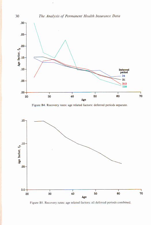
The Analysis of Permanent Health Insurance Data
ne. Figure 84. Recovery rates: age related factors: deferred periods separate.
Flgure B5 Recovery rates age related factors all deferred penods combined

Part B: Claim Recouerj~ and Mortality Intensities 31
following an inspection which gave no reason to distinguish 'run-in' periods in the case of these factors. The variables have not been subjected to transformation in these graphs. The general appearance is of a broadly linear relationship of the factors with age, and no great disparity between the deferred periods. That
U - A .
only approximately 0.5 of the grand total exposed to risk, with all but 30 of the 152 recoveries in that age group occurring under D1. No simple transformation of the variables was found which would straighten the line further.
3.5 In the light of the foregoing investigations, it was thought that, apart from the need to recognise the peculiarities of the run-in periods under D4, D13 and D26, the experience for different deferred periods seemed insufficiently different to necessitate keeping them separate. There are, indeed, strong practical incentives to combine them: to gain the stability of larger numbers, and the simplicity of having one data set instead of four or five. It was therefore decided at this point to proceed with combined data, except for keeping the first four weeks of claim separate for each of D4, D13 and D26.
3.6 Although the investigations described above give an insight into the main age and durational effects, the provisional idea, put forward in $3.2, of a multiplicative model to represent recovery rates, requires more careful examin- ation. Using values for the f, and g, factors recalculated for the data combined as described in 53.5, an estimate of p,,,;, and hence of the expected numbers of recoveries, was found for each data cell. Examination of the differences of actual from expected numbers reveals unfortunately a non-random distribution of signs of deviations, showing that the simple multiplicative model fails to fit the experience sufficiently well. A more detailed examination of the variation in observed recovery rates with age at sickness inception, while not invalidating the finding in $3.4 of a broadly linear trend with age, showed that the slope of the trend, instead of being constant, varies with sickness duration. After the first few weeks of sickness, during which the (negative) slope reduces, the slope then increases with sickness duration, and appears to be roughly proportional to the square root of duration. Consequential adjustments are therefore required to the multiplicative model if it is to form the basis of a graduation formula.
4. RECOVERY INTENSITIES-GRADUATION
4.1 The investigations described above suggested that a basic formula from which to start in seeking a suitable graduation formula would be
px+z,z = { a + b ( z ) . ( y - j ) } . (4 where a and c are constants, but h is dependent on z, reflecting the association described in 53.6.

32 The Analysis of Permanent Health Insurance Data
4.2 Attempts, during graduation trials, to find a single simple mathematical form for b(z) to represent its variation over all durations were not fruitful, and for the purpose of this basic formula it was decided therefore to cope with the main range of medium to longer durations, by letting b(z) = b.,/z, (b being a constant), leaving the short durations of the first four weeks of sickness to be dealt with by a special adjustment.
It was convenient to substitutej = 50, a round number near to the true mean. The basic formula may thus be restated:
4.3 Whilst the latter formula may be suitable for graduating much of the data, modifications are needed to cope with the three special features identified earlier:
(i) The lowered recovery rates during the run-in periods of D4, D1 3 and D26, (ii) The increased gradient of p,.,,, with respect t o y for. say, wz < 4 weeks,
and (iii) The change in gradient of p,,,:,; with respect to z for ; > 1 year.
It was found that (i) could he covered reasonably well by assuming for each of D4, D13 and D26 that p,,,,; at the moment of claim commencement (when the value of wz is equal to the deferred period) is a proportionp of the value of p,, , , calculated from the basic formula, and that the proportion increases at a uniform rate up to unity over the first 4 weeks of claim. The value o fp is taken to be the same for all ages at sickness commencement and for all of these deferred periods. The reduction factor is therefore
r = p + ( W - d ) . ( l p ) / 4 for wz < d + 4
a n d r = 1 f o r w z > d + 4
where d is the deferred period expressed in weeks. A similarly simple adjustment factor was introduced to deal with (ii). though,
in this case, what is needed is a multiplier applying to the coefficient h, rather than to the whole formula. The chosen factor is (I +q. [4 - wi]), where q is a positive constant for wz < 4, and q = 0 for wz > 4.
It was thought desirable to limit the applicable period of this factor to a maximum of four weeks, so as not to overlap the start of D4 claims. Fortunately, a period of four weeks proved quite suitable.
As previously remarked, there is little data for sickness durations exceeding two years and it would perhaps he of little practical consequence and quite expedient if any adjustment in respect of (iii) were ignored. However, there are enough recoveries in the period 1-2 years to be statistically influential in a graduation, and it was felt unreasonable to ignore the departure of the recovery rates in that period from the trend of shorter durations. It was observed that the reduction in the rate at which recovery rates declined, after the first year of

Part B: Claim Recovery und Mortality Intensities 33
sickness, could be represented roughly as equivalent to a slowing down in the passage of time itself. Thus, in entering the basic formula for sickness durations of more than one year, an adjusted value of z should be used, Z = 1 + S. (z - 1 ), where s is a constant (approximately equal to 1!3), whose value is to be fitted in the graduation.
However, for convenience in the use of the graduated rates in the overall model, it was assumed that, after five years of sickness (i.e. for z > 5 ) , recovery intensities depend on attained age only.
4.4 The complete formula used for the graduation may now be stated as follows:
where
(a) y is exact age (in years) at the date of falling sick, and
Y = y for z 5, Y = y + z - 5 f o r z z 5 ;
z is duration of sickness (in years) and
Z = z for z l _ Z = l + s . ( z - l ) f o r l < z < 5 , Z = 1 + 4,s for z > 5;
(b) for D4, D13 and D26 only,
r = min (p + ( l $ s i - d)(1 - p)/4,1) so that r = I if W: > d + 4
(c) a, h, c , p , q , s are constants.
4.5 The graduation formula is not intended for extrapolation to attained ages (y+z ) above age 65. If it were so used, then any negative values of p,+,, appearing at ages over 65 should be set to zero.
4.6 The graduation formula was fitted by the method of maximum likelihood. A general explanation of the method is given by Forfar, McCutcheon and Wilkie (1988). The estimated standard errors of the parameter estimates quoted below were obtained by a method of simulating the experience and the parameter fitting process, and, although not claimed to be very accurate, were found to be quite consistent with estimates alternatively derived by approximate calculation of the theoretical values obtainable as an asymptotic result of the theory of maximum likelihood estimation. In comparison with the standard errors, it is clear that all six parameters are significantly different from zero or unity (as the case may be) and should therefore be retained in the graduation formula.

Exact age y at falling sick
Exact duratmn of sickness
Weeks 0 I 2 3
Table E l . Graduat~d r~alues of p,,,,,
Run in penod: D4 3.4689 3.0775 2.6861 59713 5-2375 45038 78863 68491 581 19 9.3697 80662 67626
Run in prrrod D13 13744 11377 09010 24987 2.0579 1.6171 34519 28292 22066 42601 34758 2.6914

Exact age ,v at filling sick Enact durilliun oC sickness
Weeks
Years I
Table B1 (Cunlinurd)

36 The Analysis of Permanent Health Insurance Data
The fitted values of the parameters, and their estimated standard errors (given in parentheses) were as follows:
a 51.057202 (1.200) p 0.2051 11 (0.024) b 2.687089 (0.124) q 1.419428 (0.080) C 4.914441 (0.038) S 0.362456 (0.029)
4.7 A comparison of actual recoveries with those expected, based on the graduated recovery intensities, is given in Table B4. To facilitate appraisal, the results shown there have been grouped sufficiently by age and by sickness duration to ensure that there are generally not fewer than 5, and usually at least 10, expected recoveries in each cell. As a test of goodness of fit, a value for was calculated for all the results as shown in Table B4(e), i.e. for Tables B4(a), B4(b), B4(c) and B4(d) together. The value found was 224.7. Having regard to the number of cells, 202, and the fitting of 6 parameters from the data, this is not statistically significant.
4.8 Table B1 gives values of the graduated p,,:,, for specimen exact values ofy and z.
In view of the relatively low representation of lives under age 25 in the investigation, the recovery intensities shown in the table for age 20 at sickness inception should be treated with circumspection.
It may be noticed that there is a slight kink at durations 3 and 4 weeks in the run of rates for age 60. This no doubt is an anomaly arising from the rather crude adjustment in the graduation formula, by means of the parameter p, for the transition intensities in the first 4 weeks of sickness. It, was not felt sufficiently severe to compel a revision of the graduation.
4.9 For convenience of description later in this Report, the graduated rates p,,,, (excluding those for the run-in periods) are referred to as deferred period 1 week rates.
5. MORTALITY INTENSITIES-INVESTIGATION
5.1 The relatively small number of deaths precluded a detailed breakdown of the data by deferred period and sickness duration. The data for all deferred periods was therefore combined, there being no apparent distinguishing features which would necessitate their separation. The age and duration factors were examined by the same method as for recoveries, by fitting marginal coefficientsf, and g,, on the assumption of simple multiplicative effects.
5.2 It amears from the e r a ~ h of duration-related coefficients (Figure B6) that the force b i rno r t a~ i t~ tends td rise from the start of sickness to a peak after about four months of sickness, after which it declines fairly rapidly. The graph indicates an eventual upwards turn in mortality at long durations, perhaps reflecting a reversion to a dependency primarily on attained age, once the short to medium term effects of sickness on the level of mortality have worn off.
5.3 There is a strongly rising trend by age at start of sickness, as shown by the age-related factors in Figure B7, but with only a small number of deaths below age 40 it is difficult to judge the precise shape of the underlying curve.

Part B: Claim Recocery and Mortality Intensifies
Figure 8 6 . Mortality rates: duration related factors: all deferred periods combined.
.OW I I I I I I
20 30 40 50 60 70 rise
F w r e 87. Morlalily rates: aze related factors: all deferred periods combined.
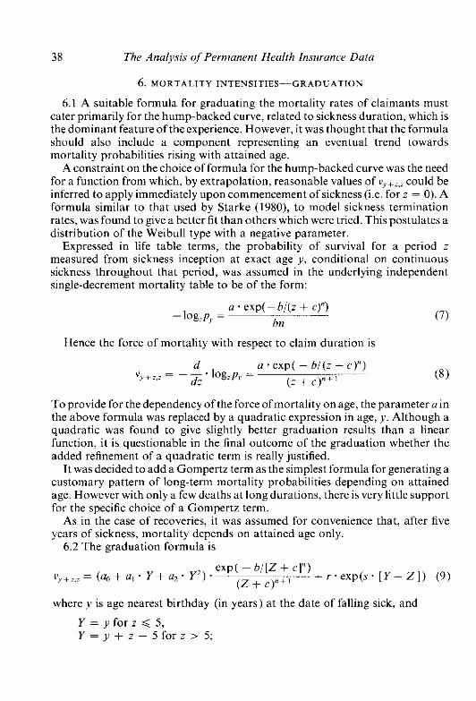
38 The Analwis of Permanent Health Insurance Data
6 . MORTALITY INTENSITIES-GRADUATION
6.1 A suitable formula for graduating the mortality rates of claimants must cater primarily for the hump-backed curve, related to sickness duration, which is thedominant feature ofthe exnerience. However. it was thought that the formula
U
should also include a component representing an eventual trend towards mortality probabilities rising with attained age.
A constraint on the choice of formula for the hump-backed curve was the need for a function from which, by extrapolation, reasonable values of v,,+,;could be inferred to aoolv immediatelv uoon commencement of sickness (i.e. for z = 0). A formula sim;ia; to that use; dy Starke (19801, to model sickness termination rates, was found to givea better fit than others which were tried. This postulates a distribution of the Weibull type with a negative parameter.
Expressed in life table terms, the probability of survival for a period z measured from sickness inception at exact age y. conditional on continuous sickness throughout that period, was assumed in the underlying independent single-decrement mortality table to be of the form:
a . e x p ( b / ( z + c)") -log,p, =
hn (7)
Hence the force of mortality with respect to claim duration is
To provide for the dependency of the force of mortality on age, the parameter a in the above formula was replaced by a quadratic expression in age, J . Although a quadratic was found to give slightly better graduation results than a linear function, it is questionable in the final outcome of the graduation whether the added refinement of a quadratic term is really justified.
It wasdecided to adda Gompertz term as thesimplest formula for generatinga customary pattern of long-term mortality probabilities depending on attained age. However with only a few deaths at long durations, there is very little support for the specific choice of a Gompertz term.
As in the case of recoveries, it was assumed for convenience that, after five years of sickness, mortality depends on attained age only.
6.2 The graduation formula is
e x p ( b : [ Z + c]") L; +;,, = (a, + a, . Y + a,. Y') .
( Z + c)"+' + r . exp(s . [ Y + Z ] ) (9)
where y is age nearest birthday (in years) a t the date of falling sick, and
Y = y for z S, Y = y + z - S f o r z > 5 ;

Part B: Claim Recoverj, and Mortality Intensities
and z is duration of sickness (in years) and
Z = z for z 5, Z = 5 for z > 5.
6.3 Fitting by the method of maximum likelihood gave the following values for the parameters, with approximate estimates of their standard errors given in parentheses:
Table B2. Graduated values of 10,000 v , , , ,
Exact agc at falling sick
Exact duration of sickness Weeks
0 1 2 3 4
5 6 7 8 9
10 I1 12 13 14
15 20 25 30 40
Years I 2 3 4 5
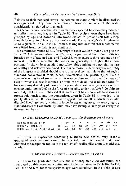
40 The Analysis of Permanent Health Insurance Data
Relative to their standard errors, the parameters r and s might he dismissed as non-significant. They have been retained, however, in view of the wider considerations referred to previously.
6.4 A comparison of actual deaths with those expected, based on the graduated mortality intensities, is given in Table B5. The results shown there have been grouped by age and duration into broad classes to provide cell totals large enough for meaningful comparisons to be made. The value of calculated on the 23 cells given in Table B5 is 13.3, which, taking into account that 8 parameters were fitted from the data, is not significant.
6.5 Graduated values of v,+: for a range of exact values o fy and z are given in Table 82. After sickness duration of 5 years, the graduated force ofmortality is a function only of attained age, and Table B3, which gives such values, may be of interest. It will be seen that the values are generally far higher than those customarily shown by a standard mortality table applying to a population base
standard conventional table. Since, nevertheless, the possibility of such a comparison may be of some interest, it may be observed that over the range of
constant addition of 0:02 to the force of mortality under the ~1967-70 ultimate mortality table. It is emphasised that no attempt has been made to discover a precise relationship, and the comparison given in Table B3 is intended to be purely illustrative. It does however suggest that an office which calculates disabled lives' reserves for claims in force, by assuming mortality according to a standardassured livesmortality table, may have an implicit margin of strength in its reserving basis.
Table B3. Graduated ~a lues of 10,000 v,,,, for durations orer 5 years Attained enact age (g+; ) 25 30 35 40 45 50 55 60 65 10,OW v , , (far : > 5) 154 171 190 213 239 269 303 342 386 lo.oou(g~+,+O-02)(A1Y67-70ult.) 207 206 208 214 225 245 280 338 431
6.6 From an experience containing relatively few deaths, very reliable graduated mortality rates cannot be expected, but it is thought that those obtained are acceptable for use in the context of the disability annuity model as a whole.
7 . DISABILITY ANNUITIES-CONTINUATION TABLES
7.1 From the graduated recovery and mortality transition intensities, the graduated double decrement continuation tables contained in Table 86, for DI, D4, D13 and D26, for three specimen ages were calculated. In the tables, I(y .2)

Parr B: Claim Recovery and Mortality Inrensities 41
represents the number of claims remaining in force at exact sickness duration z out of 100,000 claims commencing at the end of the specified deferred period, for lives aged exactly y at the date of falling sick. The decrements by recovery and death in the succeeding interval of duration are designated by r(y,z) and d(y,z) respectively. As the tables are given for illustrative purposes only, they have for convenience been truncated after 10 years (or on attainment of age 65 if sooner).
7.2 Standard actuarial methods for constructing multiple decrement tables were used to calculate the tables in Table B6.
Consider a life aged y at the date of falling sick who has been continuously sick for duration z, and let the independent rates of recovery and death in the ensuing
d short interval of time h be hq;+,, and hqy+z,z. The transition intensities at duration z+h/2 may be taken as approximations to their respective mean values over the interval from z to z + h. Better approximations may he obtained if required by reducing the size of h. Hence, for recoveries,
hqir+;,: 1 - e w h ' P i + : - b : 2 . = + h ; 2 ) (l01
and similarly for deaths. Independent decremental rates were calculated by (1 O), and the corresponding
dependent rates for the interval from i to z + h were then obtained by the approximations:
h(aqp hq' ' (1 ' hqd)
h(aqId 2 hqd. (1 p i . h@) (11)
In the calculations, h was set equal to 1125th of a week for sickness durations up to one year. and equal to ljlOOth of a year for longer durations. These values were judged to he sufficiently small to give reasonably accurate results. The decrements shown in the tables for a particular week or year of sickness were the accumulated totals obtained by working step by step through that period: calculating the numbers of recoveries and deaths at each step.
7.3 It should be pointed out that for the tables in Table B6, a week is given its natural meaning of 7 days, with a year comprising 52.18 weeks. In effect, the last week of the year is allotted a length of 1.18 normal weeks. This irregularity would be unmanageable for the more complex numerical procedures described in Parts D and E. Because of the necessity for completely uniform intervals, it is more convenient in those later calculations to work in units related to a nominal week equal to exactly 1152th of a year. This difference should be borne in mind in any close comparisons between the tahles in this Part and those included in Part E.

42 The Analysis of Permanent Health Insurance Data
Tables 84. Exposed to risk undcumpuri.son ofactua1recocerie.s with those expected according to the graduated rates
Table B4(a). ANdeferredperiods, but excludin~ the run in periods o f D 4 , D13 and
Age group
Scfkncrr pcrlad 1-2 w c k i Exmrcd W rllk idr?i) .c ,"*, rcr,,,rner E * p e ~ V d rrsorcries Slandardmd dcviarion
E ~ F C ~ ~ X C ~ V ~ E S
Sfnndilidisrd deviation
1.965 2.219 10,614 42 ?I 786 490 106 ? W 6
i o n I 3 5

Part B: Claim Recovery and Murtality Intensities
Table B4(a) (Continued)
Sirhrs . ornoil 18-22 weeks k x p a i c d r o r i b k ( d i i ~ 1 1.310 1.790 7.643 i , i i U 4680 5.056 5.191 Acl~val rrmorcncs I2 I 2 23 28 33 43 26 Expected rrrobenra 154 I V O 2 5 3 2Xi i 12V ? l 7 2 9 0 Srandlrdlrd deiirtian - 0 8 1 1 0 1 0 . 4 6 0 0 0 0 0 2 2.01 0 . 5 6
Ape group 2 - 3 4 3 5 4 4 45-49 50-54 15-59 60-64 All ancr

44 The Analysis of Permanent Health Insurance Data
Table B4(b). Run in period of D4 (deferred 4 weeksj
Age group 20 29 3 0 ~ 3 4 35-39 40-44 45-49 50-54 55-59 M-M Sickness pcriod 4-5 weeks
Exposed 10 risk (days) 720 1,039 1.323 1.440 1.709 1.606 1.261 772 Actual recoveries 6 20 13 I1 20 I 5 13 6 Expmted rccovcrlcs 9-9 133 l 6 0 l 6 2 179 156 113 6 4 SLandardircd dcviatian -124 184 -075 1 - 2 9 0-50 -0 15 051 -0-16
Sickness period 5 4 weeks Erposedtorisk(days) 666 912 1.207 1,332 1,590 1,506 1.194 718 Actual recoveries l 5 21 23 22 I5 I7 14 9 Erpectedrecover~er 133 170 21.0 21-5 238 207 l 5 0 S2 Standardised deuiacion 0-47 0.97 044 011 -180 -0 81 -026 028
Sickness period 6-7 weeks Exposed to risk (days) 566 801 1.030 1.122 1,451 1,37X 1,070 665 Aclual recoveries I3 13 25 33 26 22 12 6 Erpectedrecoveries 14-1 18-5 221 222 265 229 16.1 9.1 Standardised deviation -0.29 - 1.28 062 229 -0 10 -0 19 -102 l 0 3
Sickness pcriod 7 4 wcekr Exposcd 10 risk (days) 483 723 900 990 1,2M 2 2 4 971 587 Aciual recoveries I ? 10 21 20 25 ?4 l 5 14
Table B4(c). Run in period ofD13 (deferred 13 weeks)
Age group 20 34
Sickness period 13-15 weeks Exposed to risk (days) 840 Actual recoveries 6 Expffted recoveries 5-7 Standardised deviation 0-13
Sickness period 15-17 weeks Exposed to "sk (days) 758 Actual recoveries 7 Expected recoveries 8-8 Standardised deviation -0.61
Table B4(d). Run in period of D26 (deferred 26 weeksj
All Age group 20 3 4 35-44 45-54 55-64 ages
Sickness period 26-30 weeks Exposed to risk (days) 979 1.493 2,487 2,867 7:826 Actual recoveries 4 6 6 7 23 Expected recoveries 4 0 4.5 5.6 4.2 18.1 Standardised deviation 0 W 0-71 0 1 7 1.37
All ages

Part B: Claim Recoverj> and Mortality Intensifies 45
Table B4(e). Torals of tables B4(aJ-B4id) Age group 2 2 30-34 3 9 4 4 4 5 ~ 4 9 50-54 51-59 60-M All age9
All sickninr ncrlods
Table B5. E.xposed to risk and comparison of actual deaths with those expected according to the grarluated ratec, for all deferred period.7
combined
Age group
Sickness period 1-13 weeks Exposed to risk (years) Actual deaths Expected deaths Standardised deviation
Sickness period 13-26 weeks Exposed to risk (years) Actual deaths Expected deaths Standardised devialion
Sickness period 26 weeks-l year Exposed to risk (years) Actual deaths Expected deaths Standardised deviation
Age group
Sickness period 1-2 years Exposed to risk (years) Actual dcaths Expected deaths Standardised deviation
Sickness period over 2 years Exposed to risk (years) Actual deaths Expected deaths Standardised deviation
Age group
All sickness periods Exposed to risk (years) Actual dcaths Expected deaths
20-39 40-49 50-54 55-59 60-64 All ages
20-49 50-54 55-59 M 1 6 4 All ages
2&39 4&49 50-54 55-59 60-64 All ages

46 The Analvsis of Permanent Health Insurance Data
Tables B6. Graduated double decrement tables of claim ternlinarionv
Table B6(a). Deferredperiod I week Age r exact at date of ?dlllng rick
Sickncrs duration Weeks
I 2 3 4 5 6
8 9
10 I 1 12 13 14 15 I 6 17 18 19 20 21 22 23 24 25 26 27 28 29 30 3 I 32 33 34 35 36 37 38 39 40 41 42 43 44 45 46 47 48 49 50 5 I

Part B: Claim Recovery and Mortaliiy Intensities 47
S,ckncss duration Weeks Years l 2 3 4 5 6 7 8 9
10
Sickness duration
Weeks 4 5 6 7 8 9
10 II 12 13 14 I S I 6 17 18 19 20 21 22 23 24 25 26 27 28 29 30 31 32 33 34 35 36 37 38 39
Table B6(b). Deferred period 4 weeks Age r eracr at date of fal l ing sick
dig,:) 236 237 231 220 206 193 182 172 163 155 148 141 134 I28 123 I I 8 113 I08 I 04 1 00 96 93 89 86 83 80 78 75 73 70 68 66 64 62 60 58

48
S~ckners duratmn
Weeks 4 41 42 43 44 45 46 47 48 49 50 51
Years I 2 3 4 5 6
8 9
10
The Analysis of Permanent Health Inwrance Data
Table B6(b) (Continued) Age x cracl at date of fall~ng sick

Part B: Claim Recovery and Mortality Intensifies
Sickoesn duration
Weeks 13 14 I 5 16 17 18 I 9 20 21 22 23 24 25 26 27 28 29 30 31 32 33 34 35 36 37 38 39 40 41 42 43 44 45 46 47 48 49 50 51
Years I 2 3 4 5 6 7 8 9
10
Table B6(c). Deferredperiod 13 v
Age x exact at date of falling sick
reeks
I(Y,zI IW.OOO 97.885 94.974 91.507 87.682 83.979 80.715 77.821 75,241 72,931 70,852 68,974 67.271 65.721 64,307 63.01 2 61,823 60,728 59,718 58,783 57,917 57,113 56,364 55,666 55,013 54,403 53,832 53,295 52,791 52,316 51.868 51.446 51.047 50.670 50.312 49.973 49.652 49.346 49,055
48,778 40,405 36,898 34.81 1 33,249

50
Sickness duration weeks 26 27 28 29 30 31 32 33 34 35 36 37 38 39 40 41 42 43 44 45 46 47 48 49 50 51
years I 2 3 4 5 6 7 8 9
10
The Analysis of Permanent Health Insurance Data
Tables B6 (Continued)
Table B6(d). Deferredperiod26 weeks A p x exact at date of falling sick

C M I R 12 (1991) 51-78
PART C: THE GRADUATION O F SICKNESS INCEPTION INTENSITIES
SUMMARY
In this Part we discuss the graduation of the sickness inception intensity a, for DI, D4, D13 and D26. The final graduations of a, are given in 59 and are different for each of the deferred periods; in general, the longer the deferred period, the lower the value of G,.
Throughout this Part we assume the intensity of recovery for each of the four deferred periods is the graduated value of p,,: for D1 given in Part B. In $1 we describe the statistical model used to estimate and graduate a,; this has already been described in $53 and 4 of Part A. In 52 we describe the data we have used, most ofwhich can be found in C.M.I.R. 7(1984). In$53 and 4 wedescribe the way in which we have calculated the number of claim inceptions and the exposed to risk. In $95 and 6 we describe the method of graduation and the results of the preliminary graduations. For D1, D13 and D26 these preliminary graduations proved to be satisfactory and hence were regarded as final graduations. However, further investigations of the preliminary graduation of U, for D4, detailed in $7, showed it to be unsatisfactory and a re-graduation, detailed in $8, was carried out in this case.
1. THE STATISTICAL MODEL
1.1 A feature of the model described in Part A is that it requires the specification, and hence estimation and graduation. of a sickness inception intensity, denoted by U,. Intuitively, ~,.dt is the probability that a healthy individual aged X falls sick within a small interval of time dt. (Note that for this sickness to result in a claim it must last for at least the deferred period of the policy. which it may or may not do. This is the essential difference between a sickness inception intensity and a claim inception intensity or rate.)
The model for PHI assumes that u.? is a continuously varying function of the individual's age, X , but for the purposes of estimation it is assumed that U, is piece-wise constant, i.e. that a, is constant for a range of values of X , usually of length 1 year. The basic statistical model for the estimation of o, has been described in Part A $53 and 4. We give a brief summary below.
1.2 For a given deferred period, d, a given observation period and an age interval X I to x-2 over which a~r may be assumed to be reasonably constant, let
I ( x I , x ~ ) denote the number of sicknesses which start in the observation
5 1

52 The Analysis ofpermanent Health Insurance Data
period. with age at start of sickness between X, and X!, and which last beyond the deferred period of the policy,
E(x1,x2) denote the total time spent in the observation period by individuals who are healthy and aged between xl and x2,
n,,d denote the probability that an individual who falls sick at age X. will remain sick for at least the deferred period, d, of the policy; it is assumed that n,,dis r e a s ~ a b l y constant over the age interval X I to x2. (n,,d is equivalent to dp,ssin the notation of Part A),
V denote the factor by which the variance of the estimator for a is inflated by the presence of duplicate policies in the data.
For conciseness we shall denote I(x1,x3 and E(xl_x3 by l a n d E respectively. Let a and n denote the assumed constant values of a, and n,,d over the age interval xl to x2.
Then it is assumed that
I - N ( a . n . E . a . n . E . V ) (1)
which leads to
I i ( n . E ) - N(a;o. Vi(n. E)) (2)
An assumption underlying (1) and (2), in addition to the assumption of piecewise constancy of both o and n. is that the expected value of I i s sufficiently large for the normal distribution to be a reasonable approximation to the Poisson distribution. In practice we have taken this to mean that the expected value of I should be at least 10 for (1) and (2) to hold.
1.3 It should benoted that throughout this Part a unit of a'week', when used in connection withadeferred period. isalwaysassumed to be 1/52 ofa year, and not an exact seven days.
2. THE A V A I L A B L E D A T A
2.1 Formula (2) was used to produce graduated values of ux for DI , D4, D13 and D26 using the individual PHI data, males, 1975-78, Standard experience. Most of the data relevant to the graduation of a, can he found in C.M.I.R. 7 (1984). We give below a brief summary of the relevant available data.
(i) For each of the four deferred periods, C.M.I.R. 7, Table K13, gives the number of observed claim inceptions in 1975-78 by single ages. For all deferred periods claim inceptions are classified by age nearest birthday at the 1st January immediately preceding the date when claim payments commenced (which is broadly equivalent to age last birthday when claim payments commenced). For DI , which has some unique features, it was assumed that claim payments commenced at the start of the sickness rather than at the end of the deferred period. For all other deferred

Parr C: Sickness Inception Intensiries 53
periods it was assumed that claim payments commenced at the end of the relevant deferred period.
(ii) For each of the four deferred periods and for sickness durations 1-4 weeks, 4-13 weeks, 13-26 weeks, 26-52 weeks, 52-104weeks and over 104 weeks, C.M.I.R. 7, Tables K l K 4 , gives exposures for 1975-78 by single ages. (For each deferred period an exposure is given only for those sickness periods extending beyond the deferred period.) The exposure for sickness period 1-4 weeks is the total time spent during the years 1975-78 as healthy, or sick and claiming, or sick but not (yet) claiming by individuals aged x nearest birthday at the preceding 1st January (which is broadly equivalent to being aged .Y last birthday). For other sickness periods an adjustment has been made to this exposure so that new entrants do not contribute to an exposure until they have had their policies for at least the lower limit of the sickness period. The adjustment is a deduction from the exposure for sickness period 1-4 weeks. For all but the final sickness period this deduction can be expressed as:
1; . a r +h. /L where axis the sum over each of the four years of the number of policies at the start of the year for which the policyholders were either aged X nearest birthday and entered in the previous calendar year or aged ( X + l ) nearest birthday and entered between 1 and 2 years ago,
p, is the sum over each of the four years of the number of policies at the start of each year for which the policyholders were aged (X+ l ) nearest birthday and who entered in the previous year,
f ; a n d b are factors depending on the sickness period and are given below:
Sickness period f, h 4-9 week3 0-0034 00899
13 26 weeks 0-0312 0.2188 26-52 weeks 0-1250 03750 52-104 weeks 0-5000 0.5000
(iii) For each deferred period. C.M.I.R. 7, Tables K 1-K4, gives for single ages the number of weeks in the observation period spent claiming at age x nearest birthday at the preceding 1st January.
(iv) C.M.I.R. 7, Appendix F , summarises the results of an investigation into the extent of duplicates among claims in the 1975-78 (Aggregate experience) data. In particular, it gives for each deferred period an estimate of the average number of policies per life and also an estimate of V, the factor by which the variance of the estimator for a, is increased due to the presence of duplicate policies. The estimate of the average number of policies per life for D4 given in C.M.I.R. 7 is 1,128 and this, together

54 The Analysis of Permanenf Health Insurance Dafa
with the implied variance inflation factor, was the estimate used for the preliminary graduation of a,. Further investigations, see 57, indicated the possibility that this estimate should have been much higher and a figure of l .34, together with the implied variance inflation factor, was used for the final graduation of a, for D4. See $8.
(v) As will be seen later in this section, it was necessary to estimate the rate of growth of the number of policies in force for all deferred periods, except D l , preferably split by age. No precise data was available for this and we were able to estimate only a rate of growth for each of these deferred periods for all ages combined. The estimated annual rates of growth are as follows:
Deferred period Rate ofgrowth p.a. ($6)
4 weeks 6 2 13 weeks 6 8 26 weeks 3.4
(vi) For each of the deferred periods greater than 1 week we had available in 5-year age groups the number of recoveries, deaths and expiries in each of the four weeks following the end of the deferred period. This data was drawn from a data file from which duplicate policies could be, and had been, virtually eliminated. This is in contrast to items (i), (ii), (iii) and (iv) above, which were drawn from data files from which duplicate policies could not be, and had not been, eliminated.
3. THE NUMBER OF CLAIM INCEPTIONS
3.1 For DI , the number of claim inceptions, denoted I in (l), at age X last birthday was taken to be the figure given in C.M.I.R. 7, Table K13, without any adjustment. For the other deferred periods the situation was not so straightfor- ward.
3.2 The estimation and graduation of a, requires the value of n.,,,, the probability that a sickness starting at age X lasts for at least the deferred period, d, to be known. The value of n,d can be calculated from formula (27) in Part A. It can be seen from this formula that to calculate n,T,,l we need to know the values of the intensities of recovery, p, and mortality from sick, v, during the deferred period. The graduation of the recovery intensity revealed the following general features:
(i) For D1, p was, broadly speaking, a decreasing function of both age and duration of sickness.

Part C: Sickness Inception Intensifies 55
(ii) For deferred periods greater than 1 week, p increased in each of the four weeks immediately following the end of the deferred period and was then a decreasing function of both age and duration of sickness not significantly different from the experience for DI.
Feature (i) above is very much in line with our expectations for a recovery rate, but (ii) is difficult to explain in physiological terms. (A different level for p for different deferred periods could be due to different classes of life and different underwriting standards between offices, but these factors would not explain a different shape for p.) The PHI Sub-Committee took the view that the low observed values for p immediately following the end of the deferred period were due to the non-reporting of some sicknesses which lasted beyond the deferred period but ended (with recovery) within the following four weeks. (See 53.3 of Part B where it is noted that a similar feature was observed in Swedish data.) It is assumed throughout this Part that the intensity of recovery, i.e. the values of p, for all deferred periods is given by the graduated values for D1 given in Part B. Hence, for deferred periods greater than 1 week the value of I t o be used in (2) can be written:
I = I R + I N
where:
IR (=Inceptions Reported) is the number of claim inceptions given in C.M.I.R. 7, Table K13.
I N (=Inceptions Not Reported) is the number of recoveries within four weeks after the end of the deferred period which were not reported as claims or recoveries.
3.3 The value of I N at each age was calculated, or rather estimated, as follows. For a given deferred period (greater than 1 week) and one of the five-year age groups 20-24,25-29, . . . ,60-64, let E; and R , i = 1,2,3,4, denote the reported exposure (in weeks) and recoveries in each of the four weeks following the end of the deferred period. Let XR; denote the number of non-reported recoveries in each of these four weeks. The observed recovery intensity is
0, = R,/Ej i = l , 2, 3 ,4
but should have been, if the extra recoveries had been reported,
b; = (& + X&)/& + X&/2)
& = (R, + XR,)/(Ej + X& + XR$)
0; = (R, + XR2)/(E2 + X& + XR, + XRd2)
= (R, + XR,)/(Ej + X& + XR, + XR, + XRJ2)
assuming each of the extra recoveries recovered on average half way through the

56 The Analysis of Permanent Health Insurance Data
relevant week. The XR,'s can now he calculated by assuming the ratio P,/@.? is the same as the ratio of the eraduated recoverv intensities for the narticular deferred period and for deferredperiod 1 week at [he mid-point of therelevant week, i.e. by assuming:
b4/i)4 = 0.9006
bJp; = 0,7019
P; /& = 0.5032
P,,& = 0.3045
(See Part B.) (Note that the above ratios are independent of age.) The value of IN at a single age was calculated by apportioning the extra recoveries, XR, + XR2 + XR3 + XR4, for the relevant five year age group to individual ages in proportion to the exposure at these ages and then multiplying by the average number ofpolicies per life for the relevant deferred period. (This last adjustment was included to make IN consistent with IR, from which duplicates had not been excluded.)
3.4 Table C1 shows for each of the three deferred periods involved, the values of IN and IR in five year age groups. Note that the values of IN in Table Cl are those used in the preliminary graduations of U,. In particular, the average number of policies per individual for D4 has been taken to be 1.128. This estimate, and the estimated values of IN, were later revised. See $37 and 8 and Table C1 1.
Table C l . Values of IR and IN used in the preliminary graduations of U;.,
Deferred Period 4 weeks 13 weeks 26 weeks
Age group I R IN IR IN IR I N
20-24 2 5 0 1 3 0 4-5 0 3.0 0 25-29 107.0 28.7 25.5 5.5 19.5 0 3 30-34 192.5 87.2 44.0 5.9 18-5 0 3 35--39 247.0 7 7 2 73-0 11-5 26-5 5-3 40-44 270.0 74.1 91.5 11.9 37-5 3-5 45-49 305.0 8 6 7 105-5 9 2 4 3 0 3-7 50-54 2 9 4 0 7 3 3 100-5 6 6 6 9 5 5.4 55-59 210.5 58.5 78-0 4 5 7 5 0 4-6 60-64 1255 3 1 4 6 0 0 3 7 6 0 5 3.8
Totals 1.7765 5301 5825 58.8 353.0 26.9
4. THE CALCULATION OF THE EXPOSURE
4.1 For a given integer age X and a given deferred period. let TE, denote the total time spent in the observation period 1975-78 at age .X last birthday. For D l ,

Part C: Sickness Inception Intensities 57
TE, is given in C.M.I.R. 7, Table KI, as the exposure for sickness period 1 4 weeks. For D4 and D1 3, TE, can be calculated by 'unadjusting' the exposures for sickness periods 4-13, 13-26 and 26-52 weeks and 13-26, 26-52 and 52-104 weeks respectively. (This is nothing more than solving three linear simultaneous equations with three unknowns.) For D26 weeks we have only two equations with three unknowns; however, we can solve these equations by making the extra: and not unreasonable, assumption that a, equals P, at each age, in the notation of52. Let CL,denote the total time spent claiming at age xlast birthday in the observation period 1975-78. For DI , the values of CL, are given in C.M.I.R. 7, Table K 1. For deferred periods greater than 1 week we need to add to the figures given in C.M.I.R. 7, Tables K2-K4, the (very small) number ofweeks when the unreported sicknesses, as calculated in 53 above, could have been claiming. Then TE, - CL,/52.18 represents the time spent in the period 1975-78, at age xlast birthday, as either healthy or sick but not yet claiming. (Note that the exposures in C.M.I.R. 7 are measured in years whereas the time spent claiming is measured in weeks.) Letp, denote the proportion of TE, which is spent as sick but not yet claiming. Then EH,, where
represents the time spent in 1975-78 as healthy by policyholders aged x last birthday. We do not know the value ofp, but, using the numerical algorithms outlined in Part D, and provided we know the values of all the transition intensities, including a,, we can calculate for any age so the probability that a policyholder who was healthy at age xo and who is alive at exact age y ( > xo), is sick but not yet claiming at age y. (Note that we need the extra conditioning at age xo to make this a well-defined probability in terms of our model.) We denote this probabilityp(y;x~). Table C2 shows some values ofp(y;xo) for selected ages y and xo and each of the deferred periods. These values have been calculated using the final graduations of U, for each of the deferred periods. It can be seen fromTable C2 thatp(y;xo) is not very sensitive to the value of xo and hence that, for any reasonable xo, p(x+$;x,) should be a reasonable approximation to p,.
4.2 To calculate the values in Table C2 using the algorithms described in Part D we have used a step size of 1,104 of a year (see Part D g2.1) and the following function for p,:
p, = a + b x ' + exp(c+ dx')
X' = (x-70)/50

58 The Analysis of Permanent Health Insurance Data
Table C2. Values of 100,000 p(y;xo)
Deferred Period
y xo I week 4 weeks 13 weeks 26 weeks
31 20 397 499 505 318 31 30 397 499 505 318
34 20 387 513 512 328 34 30 387 513 512 328 41 30 365 526 533 386 41 40 366 527 534 387 44 30 358 533 552 432 44 40 359 534 553 432
51 40 359 591 657 613 51 50 364 597 662 617
54 40 369 650 745 741 54 50 373 654 749 744
This formula for p, is based on a graduation of male Assured Lives, 1975-78, select mortality at duration zero.
4.3 We would expect the value ofp(y;xo), for given y and xo, to increase with the deferred period, but Table C2 shows that this is not always the case. For example, the value ofp(31;xo) for xo equal to 20 or 30, is 397 X 10-I for D1 and 3 18 X 10-I for D26. The practical interpretation of these figures is as follows: for a group of D1 policyholders all aged 31, on average a proportion 397 X 10-5will be sick with a duration of current sickness less than 1 week; for a group of D26 policyholders all aged 31, on average a proportion 318 X 10-5 will be sick with duration of current sickness less than 26 weeks. An important distinction between these figures is that they have been calculated using different functions for a, (see 56); 0 3 1 is 0.3218 for D1 and 0.1 145 for D26. A helpful way of assessing the effect of thisdifference is to note that ifwe used the values of U, appropriate to DI, the proportion of individuals aged 31 whom we would expect to be sick with duration of current sickness less than 26 weeks would be just under 900 X 10-I.
4.4 For D1 the exposure E at age X in (2) was taken to be EH, as given by (3) without any further adjustment. For the other deferred periods two further adjustments were made. Let d, measured in years, be one of these deferred periods. Theclaim inceptions are recorded as age xlast bl;rthday at the start of the claim payments, which is on average at exact age (X+?-d) at the start of the sickness which resulted in the claim. Hence we require the corresponding exposure between ages (X-d) and (X+ l -d). We can approximate this by
d X E H , , + (I - d ) X EH,
Finally, the sicknesses which result in claims in the period 1975-78 are those which start in the period (1975-d) - (1978-d) and again we require the corresponding exposure. This can be approximated by

Parr C: Sickness Inception Intensities 59
(I -g)-d X ( d X EH,- , + (I - d ) X EH,) (4)
where g is the annual rate of growth of the number of policies in force for the relevant deferred period, and is given in 92.
4.5 In summary, the exposure 'at age X', E, to be used in (2) is given by (3) for D1, and by (4) for the other deferred periods. Note that the calculation of these exposures requires the calculation of the proportionsp,, or, more precisely, ofthe prohabilitiesp(x+~;xo), which in turn require a, to be known. This is adifficulty since our aim in the section is to estimate U,! We shall return to this oroblem in the next section.
4.6 Table C3 gives for each deferred period and selected ages the exposure 'at age X', E, used in (2) for the final graduation of U,. By comparing the figures in Table C3 and those given for the exuosures in C.M.I.R. 7, the combined effect of all the adjustments outlined in thidsection can he assessed
Table C3. Exposures (in Tears) af ugr X
Deferred Period
Age l r*.eek 4 weeks 13 weeks 26 weeks
30 2.847 3.254 4,716 8.787
5. THE GRADUATION PROCESS
5.1 The next stage of the graduation process, after the calculation of the inceptions, I, and exposures, E. at single ages, was the grouping of ages, if necessary, to ensure an expected number of inceptions of at least ten in each group. This produced the following age groupings:
Deferred period 1 week: single ages from 23 to 64 inclusive, Deferred period 4 weeks: single ages from 25 to 64 inclusive, Deferred period 13 weeks: ages 25 to 28 as one group and then single ages
from 29 to 63 inclusive, Deferred period 26 weeks: three year age groups from 31 to 39 inclusive,
two year age groups from 40 to 49 inclusive and then single ages from 50 to 63 inclusive
(Initially, an extra age group, covering ages 28 to 30 inclusive, was included for D26 but this gave a very high observed value for a, which distorted the graduation, particularly when the graduation of a, was extrapolated back to age 20. For this reason this age group was not used for the graduation of 0 , for D26.)

60 The Analj~sis of Permanent Health Insurance Data
5.2 The values of the probabilities n,,d were then calculated for each age group and an appropriate value of X. (For example. for age 50, n,,, was calculated at x = 50.5 for D1 and at x = 50 for D26). The values of l!n,,rE were regarded as point estimates of a,, with x taken to be the mid-point of the age interval (less the deferred period where this is greater than 1 week.) (For D13, age group 25-28, the estimate of a, was taken to be a point estimate at exact age 27: rather than exact age 262, with n,,dcalculated accordingly; this adjustment was made to take account of the unevefl incidence of exposure over this particular age group.)
5.3 After preliminary investigations it was decided that a, should be graduated by functions of the form:
0" = expl.f(x)) (5)
whereflx) is a polynomial, usually of degree 3. The combination of the chosen functional form for U,, (S), and the statistical model, (2), is ideally suited to the statistical computing package GLIM. However, a, needs to be known since it is required for the calculation of the exposures, E, and since it appears in (2) in the variance of the estimator.
To overcome these difficulties, the following iterative procedure was used:
(i) The factors p, used in the calculation of the exposure E were set at zero. The variance of the estimate in (2) was set at I. Vi(n,,dE)2.
(ii) GLIM was then used to fit, by maximum likelihood, the coefficients of the polynomial f (X).
(iii) The 'graduated' values of a, calculated in (ii) were used in the variance term in (2) and GLIM was used again to re-graduate U,.
(iv) Step (iii) was repeated until the 'graduations' of U, converged to a limit. This usually took about four GLIM runs. (In practice, u , ~ was deemed to have converged to a limit when each of the relative differences between corresponding coefficients in f (X) in successive 'graduations' was less than 10-'.)
(v) The 'graduation' of a, resulting from (iv) was used to calculate the p, factors and hence to uudate the values of the exuosures E.
(vi) Steps (iii), (iv) and (v) were then repeated until the 'graduations' of a, converged to a limit. This usually took about three or four calculations of thep, factors. (In practice, a, was deemed to have converged when a new cycle of the process resulted in the same coefficients for f ( x ) to four significant figures.) This graduation was regarded as the final graduation of U,.
6.1 The results of the graduation process described in $5 are presented and discussed in this section. Throughout this section these results are referred to as the 'preliminary graduations'. For Dl , D13 and D26 the preliminary gradua-

Part C: Sickness Inception Intensities 6 1
tions were found to be satisfactory and were adopted as the final graduations. For D4 the preliminary graduation discussed in this section was found to be unsatisfactory in one respect (see 97) and an adjustment was made to produce a final graduation. See $8.
6.2 The formula for the polynomial f (X) in (5) was chosen to be a cubic for all graduations except D26, for which f (X) was chosen to be a quadratic, i.e.
f (X) = a + hx + cx' + dx3 (6)
with d = 0 for D26. The preliminary estimates of a, b, c and d, together with the standard errors of these estimates, are shown in Table C4. (Note that the parameterisation used by GLIM makes the standard error of the parameter a irrelevant.) Tables C5, C6, C7, and C8 show for each of the four preliminary graduations and each age (or age group) used for the graduation,
(i) the estimate of o, at the mid-point of the age interval used for the graduation (less the deferred period where this is greater than 1 week),
(ii) the corresponding graduated value of a,, (iii) I, the adjusted observed number of claim inceptions for this age (or age
group) including an estimate of the number of unreported inceptions as explained in 93 above,
(iv) E m , the expected number of inceptions for this age (or age group), (v) 100I/Ena and (vi) (I-E?ICT)/(VE~T)~, which, from (I). can be regarded as a standardised
residual coming from a N(0,l) distribution.
In each case the totals of actual and expected claim inceptions are equal, apart from rounding errors. This can be shown to be a mathematical consequence of the statistical model and the graduating function specified by ( l ) , (5) and (6). Similar results are presented in Forfar, McCutcheon and Wilkie (1988, Appendix
6.3 Table C9 summarises the results of some standard tests of the preliminary graduations. This table shows a value of a 1' goodness of fit statistic, with the appropriate number of degrees of freedom (this is the scaled deviance computed
Table C4. Paran~eter estimates for the preliminary graduations
Parameter l week
il - 1.796
h 8.083 X 10 ?
Standard error of h 6-93 X 1 0 '
- 2 6 8 6 ~ 10-' Standard error of c I -60x l 0 ' d 2498 X 10-' Standard error o f d 1 . 1 9 ~ 10 '
Deferred Period
4 weeks 13 weeks 26 weeks - 4 l h 8 -2722 -4.819 n 10 '
2290 X 1 0 ~ l 2 9 0 X 1 0 -8.434 X 10-% 1-39 X 1 0 ~ 2.963 X l 0 ' 7-44 X 1 0 ~ >
6 . 2 5 8 ~ 10 ' - 4 . 2 4 0 ~ 1 0 ' 9 7 4 9 x 10-' 3 1 5 X I O W 6.57% 10 ' 7.58 X 10 '
5299 X 10-' 3.888 X 10 ' 0 2-32 X 10 ' 4-80 X 10-'

Table C5. Preliminary graduation of a, for Beferred period 1 week: esrimared and graduated values of a, and actual and
expected numbers of claim inceptions
Claim Inceptions l001 ( I - E x t d v t ) Age x Estimate Graduated Observed Expected p
I En , ,o , (VEnt ,do l )+
Totals

Table C6. Preliminary graduation of a, for deferred period 4 weeks: estimated and graduated values of ax and actual and
expectednumbers of claim inceptions
Adjusted Age x Estimate Graduated observed Expected 1M)I (l-Enxdar)
En.,da, En,,o, ( V E = , , ~ O ~ $
17.0 124-7 0.91
Totals

64 The Analysis of Permanent Health Insurance Data
Table C7. Preliminary graduation of a, for deferred period I 3 weeks: estimated and graduated ualues of U, and actual and
expected numbers of claim inceptions
Claim Inceptions
Age x
57 58 59 60 61 62 63
Totals
Estimate of 0,
Graduated a<
0.2086 02012 0.1972 0.1930 0.1887 0.1843 0,1799 0,1755 0.1711 0.1669 0 1628 01589 O.IS51 0-1516 0.1484 0.1454 0-1427 0.1403 0-1382 0.1365 0-1351 0.1342 0.1336 0-1335 0.1338 0-1347 0.1361 0.1380 0-1406 0-1440 01481 0.1531 01592 0,1664 0,1749 01851
Adjusted observed Expected
I En,.do.
17.3 16.2 137 11.4 116 10-0 10.7 11.7 13.7 12-7 8.2 13.6 5 7 140
14.8 14.2 212 1 4 5 11.7 15.1 16-3 162 20-4 174 13.0 18.4 21-9 190 19.4 19.6 21-3 20.3 27-8 210 24.0 21.7 23-4 222 198 22.4

Part C: Sickness Inception Infensities 65
Table C8. Preliminary graduation of a, for deferred period 26 weeks: estimated and graduated aalues of a, and actual and
expected numbers of claim inceptions
Claim Inceptions
31-33 34-36 37-39 40-41 42-43 44-45 46 -47 48-49 50 51 52 53 54 55 56 57 58 59 60 61 62 63 64
Totals
by GLIM, which, for our particular model, can be interpreted as a 1' value), the numbers of +'S and -'S_ where a + indicates that the estimate of a, is greater than the graduated value (or, equivalently. that the observed number of claim inceptions is greater than the expected number) and a - indicates the reverse, and the number of runs of +'S and -'S. None of the results in Table C9 indicates an unsatisfactory graduation.
6.4 A noticeable feature of Table C4 is that for D13 the estimates of h, c and d are not significantly different from zero. This suggests that one or more of these parameters could he set equal to zero. Putting d equal to zero has the effect of making the revised estimates of b and c significantly different from zero: and increasing the ;(' statistic by only 0.6 with an increase of I in the number of degrees of freedom. These are arguments in favour of setting dequal to zero. The argument against. and the reason why dwas not set equal to zero, is that while its

The Analysis of Permanent Health Insurance Data
Table C9. Tests of the graduations
Deferred Period
I week 4 weeks 13 weeks 26 weeks
X ? 42.0 41.7 28.4 14.3 Degrees of freedom 38 36 32 20 No. of +'s 22 20 20 13 No, of - 'S 20 20 16 10 No. of runs 28 21 24 15
inclusion does not significantly improve the fit over the range of the data, when the function for ar is extrapolated back to age 20, it gives a shape for a, much more in line with the graduations of a, for D1 and D4 , for which there is more data in this range of values of x than there is for D13. For D26, the estimates of b and c are not significantly different from zero; in fact, setting both b and c equal to zero. and hence fittine a constant function to a,. results in a y2 statistic of onlv 18.2with 22 degrees of freedom! This is partlya result of the relatively scan& data for D26. The parameters b and c have been included for this graduation so that the resulting function for a, has broadly the same shape as for the other deferred periods. The inclusion of parameter d for D26 not only did not improve the fit over the range of the data but also did not change significantly the extrapolated values of a, in the age range 20 to 30; for this reason d was set equal to zero in this case.
7. FURTHER INVESTIGATIONS
7.1 An important assumption in our graduation of a, is that the intensities p and v are the same for all deferred periods. A consequence of this assumption, taking account of the low observed values o f p in the four weeks following the end of the deferred period for all deferred periods except 1 week, is that some sicknesses which last beyond the deferred period and then recover within four weeks are not reported. We have estimated these 'unreported inceptions' as explained in $3 and then graduated a, using the total of reported and unreported inceptions. An alternative approach, and a useful way of checking our assumption, would be to deduct from the reported inceptions those claims which were reported to have terminated within four weeks of the end of the deferred period and regard the resulting figure as the number of claim inceptions with an effective deferred period four weeks longer than the original deferred period.
7.2 To clarify this check, consider D4; the same check was applied to D1 3 and D26. We know the number of reported claim inceptions at each age, including duplicates, since these are given in C.M.I.R. 7, Table K13. This is IR in the notation of 93. We also know the number of reported claims which terminated for any reason within four weeks of the end of the deferred period, excluding duplicates. By multiplying this last figure by the average number of policies per

Part C: Sickness Inception Intensifies 67
individual and then deducting it from IR we obtain an estimate of the number of sicknesses at each age which lasted beyond eight weeks. For a given age let us denote this figure by IR*. We can calculate the expected number of sicknesses for this age which last beyond eight weeks, denoted IE*, as
IE* =u.n'. E
where E is the same exposure as calculated in 54, U is the graduated value of U, at the mid-point of the interval less four weeks and n' is the probability that a sickness which starts at this age lasts for at least eight weeks. If all our assumptions are valid, we have
IR* - N(IE*, V . IE*) (7)
where V is the variance inflation factor to take account of the effect of including duplicate policies in both IR* and IE*. In particular, we can calculate
(i) the number of +'S, i.e. ages where IR* is greater than < IE*, and -'S, (ii) the total over all ages of both IR* and IE*,
(iii) the sum of (IR* - IE*)*/(V.IEe) , which, according to (7), has a x2 distribution with number of degrees of freedom equal to the number of ages less the number of fitted parameters in the formula for a,.
7.3 The results of these checks for each of the deferred periods are summarised in Table C10. The results in Table C10 for D1 3 and D26 are encouraging but the results for D4 are disappointing. A possible cause of the disappointing results for D4 is that the estimate of the averaee number of oolicies oer individual for this class of business is too low. (The estimate we have used is 1 .l28 and is taken from C.M.I.R. 7, Appendix F.) The effects of a higher estimate of the average number of policies per individual would be
(i) to increase IN, in the notation of $3, and hence (ii) to increase the graduated values of a,, and hence
(iii) to increase IE*, (iv) to decrease IR* by increasing the number of terminations to be deducted
from IN. Hence, the overall effect of an increase in this estimate would be to reduce IR* and increase IE*. A rough calculation, based only on totals, shows that if the average number of policies per individual were 1.34 rather than 1.128, then IR* would be approximately equal to IE*. (It is interesting to note in C.M.I.R. 7 Appendix F that an under-estimate of this factor could be an explanation of the difficulties experienced by the PHI Sub-Committee in the graduation of claim inception rates for D4.)
7.4 Although the evidence is by no means conclusive, the PHI Sub-Committee decided it was prudent to graduate a, for D4 on the assumption that the average number of policies per individual was 1.34 and not 1.128 as given in C. M.I.R. 7 Appendix F . The details of this re-graduation are given in the next section.

The Analysis of Permanent Health Insurance Data
Table C10. The effect of eliminating termina- tions within 4 weeks of the end of the deferred
period
Deferred Period
4 weeks 13 weeks 26 weeks
/R* 1.155 475 298 /E* 998 459 317 X: 115.7 38.0 16-8 Degrccs of freedom 36 32 20 No. of + ' S 28 22 10 No. of ' S 12 14 13 No. of runs l7 23 16
8. THE REGRADUATION OF U, FOR DEFERRED PERIOD 4 WEEKS
8.1 As explained in the previous section, the PHI Sub-Committee decided it W-ould be prudent to re-graduate U, for D4 on the assumption that the average number of policies per individual was 1.34. Using the distributional assumptions outlined in C.M.I.R. 7 this implies that the variance inflation factor V in (1) should be 1.68 rather than 1.26.
8.2 A consequence of these new assumptions is that the estimates of IN, the number of sicknesses assumed to be not reported, have to be revised (by multiplying by a factor 1.34!1.128). The revised figures are given in Table C11 The figures in Table C1 1 should be compared with those in Table C l .
Table C I 1. Reported and non-reported claim incep- tions for deferred period 4
weeks
Age group / R IN
20-24 25 154 25 29 107 34. l 30-34 1925 1036 35 39 247 91.7 40-44 270 88.0 45-49 305 1030 50-54 294 87.1 55-59 210.5 69.5 60-64 l 2 5 5 3 7 3
Totals 1,7765 6297

Part C: Sickness Inception Intensities 69
8.3 The function used to re-graduate U , was, as for the preliminary graduation. of the form
U , = exp(a + hx + cx' + d x 3 ) (8)
The final estimates of the parameters together with their standard errors are given in Table C12. The figures in Table C12 should be compared with the corresponding results for the preliminary graduation, which are given in Table C4.
The results of standard tests of the graduation together with actual and expected values corresponding to Tables C9 and C6 are given in Tables C1 3 and C14 respectively.
8.4 The results of the tests of the graduation summarised in Table C13 are satisfactory. The graduation was further tested, as in 97, by eliminating terminations within four weeks of the end of the deferred period. The results of this test are given in Table C15 using the same notation as in 57.
8.5 The outstanding feature of Table C15 is the very high X' value. (Note that the number of degrees of freedom is not very clear since not only have four parameters been fitted from the data but IE* has been constrained to be approximately equal to IR*. We have taken account of this by reducing the number of degrees of freedom by one.) A large contribution to this X' value comes from a few ages, notably 26, 54 and 64 where the number of claim inceptions is very much higher than expected, and a few ages, notably 40 and 62, where it is very much lower. This feature can be observed in the number of reported claim inceptions as given in C.M.I .R. 7 Table K13. This feature did not give a large x2 value for the re-graduation of U , (see Table C13). or for the
Table C12. Parameter esfirnates and standard errors for the re-graduation of
o x f o r deferredperiod 4 x~eeks
Parameter Estimate Standard Error
U -4256 b 2 . 3 9 2 ~ 1 0 ' 1 . 5 6 8 ~ I O W
C - 6 . 4 9 8 ~ I O W 3561 x 1 0 ~ ' d 5 4 7 6 x 10 ? 2623 X 10 '
Table C13. Tests of the re-graduation of U , for dejerred period 4 weeks
X: 3 0 6 Dearees of freedom 36 . No. of + ' S 20 No. of -'S 20 No. of runs 21

Table C14. Re-graduation of a, for deferred period 4 nseeks: estimated and graduated values of a, and actual and expected
numbers of claim inceptions
Claim Inceptions Adjusted
Age x Estimate Graduated observed Expected
Totals

Part C: Sickness Inception Intensifies
Table C15. The effect of eliminating terminations within 4 weeks of the end of
the deferred period
IR* 1,043 /E * 1,044
L' 67.7 Degrees of freedom 35 N o of +'S 20 No. of - ' S 20 No ofruns 23
preliminary graduation (see Table C9), because by smoothing the values of IN over five year age groups and then adding them to IR, any unevenness in the individual values of IR becomes relatively less important. The reverse is true when smoothed values are deducted from IR to obtain IR*. This seems to be the explanation for the large x2 value in Table C15.
In the circumstances the PHI Sub-Committee regarded the re-graduation of a, for D4 as a satisfactory final graduation.
9. CONCLUSIONS A N D FURTHER COMMENTS
9.1 The PHI Sub-Committee regard the preliminary graduations of a, for D1, D13 and D26, as given in $6, and the re-graduation of U, for D4, as given in 58, as satisfactory final graduations.
In summary, the final graduations of a, for the four different deferred periods are:
Deferred period 1 week
U, = expi-1.796 + 8.083 X 10⁻² X X-2.686 X 10-' X x2 + 2.498 X 10-S X X') (9
Deferred period 4 weeks
U, = exp{-4.256 + 2.392 X 10-' X X-6.498 X 10 X x2 + 5.476 X 10-S X X'} (10)
Deferred period 13 weeks
a, = expi-2.722 + 1.290 X 10-' X X-4.240 X 10-3 X x2 + 3.888 X 10-' X x3) (11)
Deferred period 26 weeks
ax = exp{-4.819 X 10-'-8.434 X 10-' X X + 9.749 X 10⁻⁴ X X') (12)
Graphical summaries of the final graduations for DI, D4, D13 and D26 are shown in Figures Cl. C2, C3 and C4, respectively. In particular, these figures

- - Yinw 2 s.e.
-
-
-
-
-
-
- F -
- 20 25 30 35 40 45 50 55 60 65
- Obaarsed lnrluea
Plua 2 ss.
nge Figure Cl . Sickness inception intensities: deferred period I week.
- Graduated rates
0.6-
0.5-
0.4- 3 g J
0.3- A i
0.2-
2 0.1-
0.0-
Aw Figure C2. Sickness inccprion intensitien: deferred period 4 weeks.
- - Yinw 2 ss.
. . ..
l. ! '\'
I I I I I I I-- 20 25 30 35 40 45 50 55 60 65
+- Obssrpsd value.
Plua 2 i.e. - Graduatad mtm

- - Uin~m 2 %c. -r Obamed - Plus 2 a.e. - Graduated value8 ratea
irse Figure C3. Sickness inception intensities: deferred period l 3 weeks.
I I I I I I I 1 25 30 35 40 45 50 55 60 65
Figure C 4 Sickness inception intensities: deferred period 26 wceks.
. - Uinw 2 a.e. . . -. Plus 2 8,s. - 0-d valuea
- Graduated ratss

74 The Analysis of Permanent Health Insurance Data
show the final graduation, the point estimates of a, and the point estimate 2 standard errors.
9.2 Table C16 gives graduated values of a, at selected exact ages X for each of the deferred periods. It may be seen from these figures that. apart from some slight aberrations between ages 20 and 30, where the data is relatively scanty, the functions have the same general shape, with a minimum at about age 50. It is tempting to speculate on why a sickness inception intensity should have such a shape, or even whether such a shape is reasonable. However, care should be exercised in such speculation. The estimates of a, given in Tables CS, C7, CS, and C14, and hence the final graduations of a,, depend very much on the assumed values for the intensities p and v for durations of sickness within the deferred period, values which are the result of a (not unreasonable) extrapolation exercise. To ~ u t it another W-av. changes in the values of o and v for durations of sickness , , U
within the deferred period which resulted in the probabilities n increasing by a constant factor would, broadly speaking, result in the estimates and graduated values of ax decreasing by the same factor, without any change to the expected number of claim inceptions. A more reasonable object of speculation is the product o;n,d. Intuitively, a,.n,,ddt is the probability that a healthy individual aged X falls sick in a small interval of time dt and remains sick for at least the deferred period of his policy. Hence o,.nx,d represents a claim inception intensity to be applied to healthy individuals. Table C17 gives values of ox-n,.dfor selected exact ages X and each deferred period.
Table C16. Graduated values of a,
Deferred Period Age .X l week 4 weeks 13 weeks 26 weeks
20 0.3486 01953 0-2172 0-1689 25 03452 02273 0-2145 01379 30 0.3282 0.2346 0.1982 0.1183 35 03054 02240 0-1766 0-1065 40 02832 02059 0-1560 0-1007 45 02667 01901 0-1408 0-1000 50 0,2600 01834 0.1337 0.1042 55 02673 01929 0-1375 0 1 140 60 02952 02302 01576 0.1310 65 0.3569 0-3251 02073 0-1580
9.3 The values of a,.n,.,, given in Table C1 7 can reasonably be compared with the graduated claim inception rates given in C.M.I.R. 7, Table H5. The former are, in general, a little higher for two reasons:
(i) the exposure appropriate to a,.n.r.d is time spent as healthy at age X, which is less than the exposure to which the graduated inception rates in C.M.I.R. 7 are designed to be applied,
(ii) for all deferred periods other than 1 week, the values of a, have been based

Part C: Sickness Inception Intensities
Table C17. Values of 10,000 o,.n,,d
Deferred Period
Age X l week 4 weeks 13 weeks 26 weeks
20 1,164 797 1075 2246 25 1,237 117.9 15.49 2965 30 1,262 1559 2087 4105 35 1,260 1906 27.13 5-975 40 1,254 224.6 34.91 9.113 45 1,267 2654 4589 1458 50 1,325 3280 6343 2446 55 1,461 441.7 94.89 43.00 60 1.732 6750 1582 79.32 65 2,246 1,220.0 3023 1534
on claim inceptions, both reported and unreported; the claim inception rates in C.M.I.R. 7 were based only on the reported inceptions.
9.4 A feature of the graduated values of a,, as shown in Table C16, is that, although a, has the same basic shape for each of the deferred periods, the values of U, decrease as the deferred period increases. (This is not strictly true for D4 and D13 at the youngest ages, but this is an area where there is little or no reliable data.) It is of interest to check whether the differences between the sickness inception intensities for different deferred periods are significant. The answer to this question is already reasonably clear. particularly for the shorter deferred periods, and can be seen by comparing the point estimates of U, given in Tables C5, C7. C8 and C14. Comparing the estimates in Tables C5 and C14 we can see that the estimate of a, for D4 is less than the corresponding estimate for D1 at every age except age 64. More formally we can check whether the data for one deferred period is consistent with the graduated values of ux for a different deferred period. If not, then we have been justified in graduating separately for these different periods. To clarify this, consider D1 and D4. At each age we have an observed number of claim inceptions, denoted I, for DI. Using the graduated values of a, for D4 we can c?lculate the expected ;urnhers of claim inceptions for D1 at each age, denoted IE. We can calculate IE using the formula
I E = U . X . E where U is the appropriate value of a, using the graduation for D4, n is unchanged and the exposure E i s calculated as in 54 with the exception that the factorsp, are calculated using the graduated values of U, for D4. If the data for D1 is consistent with the graduation of a, for D4, we would have for each age
I - N(IE, v . [E) (13)
9.5 Table C18 shows the results of testing the data for D1 and D13 against the graduation of o, for D4. The results shown in Table C18 are

76 The Anal?.sis r,fPermanent Health Insurance Data
(i) the totals of I and &over all ages included in the graduation of U~ for D1 or D4.
(ii) the number of +'S, ages where I is greater than I& and -'S, (iii) the total over all ages of ( I - I E ) 2 / ( ~ . f ~ ) , which, if (13) holds, has a
distribution with number of degrees of freedom equal to the number of ages.
Table C18. Testing the data for deferredperiod I week and 13 weeks against the ~raduured 1:alues of U ,
for deferred period 4 weeks
Deferred Period
l week 13 weeks
I 11.068 633 / E 8.070 851
f 5627 7 0 4 Dcgrccs of frccdom 42 36 Number of + ' S 42 3 Number of - ' S 0 33 Number of runs I 7
9.6 Table C19 shows the results of testing the data for D4 and D26 against the graduated values of a, for D13. These two tables show very clearly that there are significant differences, in terms of the values of U,, between the data for different deferred periods and, in particular, that assuming all our other assumptions are valid, notably that the intensities p and v do not depend on the deferred period, the sickness intensity decreases as the deferred period increases.
9.7 The magnitude of the differences between the graduated values of a, for
Table C19. Testing the data for deferred periods 4 w r k s and 26 n,eeks against the graduated vo/ue.s o f a, for &/'erredperiod 13 w r d . s
Deferred Period
4 weeks 26 h,eeki
I 2.365 340 / E 1.782 367
%' 1623 3 6 0 Degrees of frcedom 40 24 Number of -'S 38 I Number o f t 2 23 Number uf runs 3 3

Parr C: Sicknew Inception Znfensltie.s 77
3: 1. However, the evidence for a substantial difference between D1 and D26 in the 1975-78 data can be seen in C.M.I.R. 7. From Tables K1 and K4 it can be
fiiures is almost exactly 3:l. 9.8 Having established that this difference exists, at least in the 1975-78 data, it
is then necessary to explain. in terms of the model, how it arises. Broadly speaking. there are two possible explanations for this difference:
(a) the sickness inception intensities for D1 and D26 are the same, but the intensities of sickness termination (i.e. of recovery plus mortality from sick) in the first 26 weeks of sickness are different,
(b) the intensities of claim termination in the first 26 weeks of sickness are the same for D1 and D26 but the sickness inception intensities are different.
9.9 To investigate explanation (a) above a little more closely, let u,"jand u, '~~' denote the sickness ince tion intensities at age xfor D1 and D26 respectively and let b.$ + v f i j and (p& + denote the intensities of claim termination for D1 and D26 respectively. Let 711' 'denote the probability that a sickness starting at agex lasts, for a policyholder having a deferred 26 weeks policy, for at least 26 weeks, i.e.
I 2
yt = exp(J(p,+,., ,261 + " ( 2 6 ) . ,+7, :k~~) 0
Let us assume that D!" = U:*" for all s and also that the common value is as for D1 in Table C16. Let us assume also that ut"'.n!'"is as shown for D26 in Table C17. In other words, we are assuming that the sickness inception intensities for D1 and D26 are the same (and equal to the graduated values for D l ) and that the 'claim intensity' for D26, the product uX.n,,, is as in Table C17 for D26. These assumptions are not consistent with the intensities of claim termination being the same for D1 and D26 in the first 26 weeks of sickness. It is clear that (p?,6' + v:??) must he higher than (pl!l' + v: ' ) but how much higher? In an attempt to quantify this let us assume that there is a function k(?) such that
( p L2:Lz + vjZh\,;) = ~ ( x - z ) . ( p ~ ' ! ~ , ~ + i.e. for sickness starting at age y there is a constant ratio, k ( y ) , between the sickness termination intensities for DI and D26. We can calculate k p ) from the figures givenin Tables C16and C17 and the assumption that u?~'.~!,~'Is asglven in Table C1 7. These calculations show that the values of k(y) increase from 1.1 1 at age 20 to 1.29 at age 60, i.e. broadly speaking, the sickness termination intensity for D26 must be between 10% and 30% higher than for D l , in the first 26 weeks of sickness. if the sickness inception rates for these two deferred periods are to be the same.
The difficulty with adopting this explanation for the difference in experience between D1 and D26 is that there is insufficient data to reveal significant

78 The Analysis of Permanent Health Insurance Data
differences in the sickness termination intensities after 26 weeks of sickness between D1 and D26 other than the run-in period. For this reason the PHI Sub- committee decided to assume that the sickness termination intensities for D1 and D26 (and also D4 and D1 3) were the same both before and after 26 weeks of sickness. In other words, the PHI Sub-Committeedecided to explain the whole of the difference between D1 and D26 in terms of the sickness inception intensity, a,. The result is the set of values of 0, shown in Table C16.
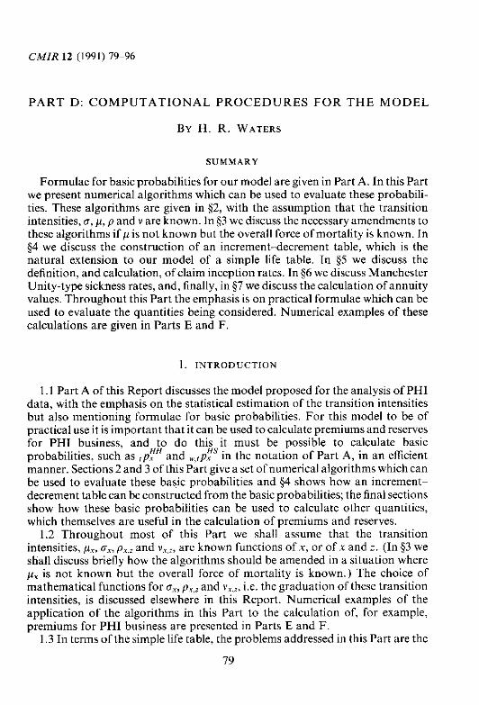
CMIR 12 (1991) 79-96
PART D: COMPUTATIONAL PROCEDURES F O R T H E MODEL
S U M M A R Y
Formulae for basic probabilities for our model are given in Part A. In this Part we present numerical algorithms which can be used to evaluate these probabili- ties. These algorithms are given in $2, with the assumption that the transition intensities, o, p, p and v are known. In 53 we discuss the necessary amendments to these algorithms if pis not known but the overall force of mortality is known. In $4 we discuss the construction of an increment-decrement table, which is the natural extension to our model of a simple life table. In 55 we discuss the definition, and calculation, of claim inception rates. In 56 we discuss Manchester Unity-type sickness rates, and, finally, in 57 we discuss the calculation of annuity values. Throuehout this Part the emnhasis is on oractical formulae which can be used to evaluate the quantities being considered. Numerical examples of these calculations are given in Parts E and F.
1. INTRODUCTION
1.1 Part A of this Report discusses the model proposed for the analysis of PHI data, with the emphasis on the statistical estimation of the transition intensities but also mentioning formulae for basic probabilities. For this model to be of practical use it is important that it can be used to calculate premiums and reserves for PHI business, and to do this it must be possible to calculate basic
HH HS . probabilities. such as , p , and ,,,p, in the notation of Part A, in an efficient manner. Sections 2 and 3 of this Part give a set of numerical algorithms which can be used to evaluate these basic probabilities and $4 shows how an increment- decrement table can be constructed from the basic probabilities; the final sections show how these basic probabilities can be used to calculate other quantities, which themselves are useful in the calculation of premiums and reserves.
1.2 Throughout most of this Part we shall assume that the transition intensities, ox, px.7 and v .,;, are known functions of X, or of x and z. (In 53 we shall discuss briefly how the algorithms should be amended in a situation where p- is not known but the overall force of mortality is known.) The choice of mathematical functions for U,, p,,, and v,,:, i.e. the graduation of these transition intensities, is discussed elsewhere in this Report. Numerical examples of the application of the algorithms in this Part to the calculation of, for example; premiums for PHI business are presented in Parts E and F.
1.3 In terms of the simple life table, the problems addressed in this Part are the
79

80 The Analysis of Permanent Health Insurance Data
numerical evaluation of basic probabilities, such as ,p,, and subsequently the evaluation of annuities and assurances, given the force of mortality, px. However, while there is a very simple formula for ,p, in terms of p,, viz.
,px = exp{ - j ~ ~ + , d s ) 0
the formulg;for the basic probabilities for the PHI model described in Part A, such as , p , and can be regarded as simultaneous integro-differential equations. The numerical solution of these equations requires a little care. The general method of solution of these equations, as described in this Part, has been described briefly, and exemplified in relation to the simple life table, by Waters and Wilkie (1987).
2. NUMERICAL CALCULATION OF PROBABILITIES
HH HS 2.1 In this section we show how basic probabilities, such as ,p , and ,,,,,p, , can be evaluated numerically when the transition intensities p,, a,, p , : and v,,are known functions of X, or of X and z. More precisely we consider for an individual who is healthy at some initial age, xo say, the probabilities that at some later age,
HH X , he is healthy, .-,p,, , or that he is sick with duration of sickness between ( m 1)h and mh,
"C m . - (m-l)h.x-x,,Px,,
where m = 1, 2 . . . and h is the 'step size' for the numerical algorithms. It is convenient to choose a value for h such that h-' is an integer multiple of 52, and in the applications later in this Report we shall usually take h to be 11156. In general, the smaller the value of h the more accurate the numerical procedures, and also the longer the computer time necessary to perform them; halving the value of h roughly quadruples the computer time necessary.
2.2 At this stage it is convenient to introduce a notation different from that used in Part A. We define pH(x) , p S ( x ) , p D ( x ) and pS(x ,m) as follows:
p H ( x ) = 0 ) FfS p S ( x ) = .- ,, ."P," ( 2 )
= . . ,P~Y (3) H5 H S
pS(x ,m) = M & , , ,pro ( m - 1 1 1 1 . ~ ~ ~ X~P"" (4)
for any X 2 xo and m = 1, 2, . . . , so that p H @ ) is the probability of being healthy at age X ,
pS(x ) is the probability of being sick at age X ,
p D ( x ) is the probability of being dead at age X ,
pS(x ,m) is the probability of being sick at age X with duration of sickness between ( m l )h and mh,

Part D: Compututionul Procedures for the Model 8 1
with all probabilities conditional on being healthy at the initial age xa. Note that
pS(x) = CpS(x,nz) m
Tt is convenient also to put: pDH(x) is the probability of being dead at age X, having died as healthy, pDS(x) is the probability of being dead at age X, having died as sick, with
pD(x) = pDH(.x) + pDS(x). Tt will also be convenient to have a different notation for the transition intensities and so we define functions s(x), m(x), r(x,m) and n(x,m) as follows:
s(x) = U, ( 5 )
m(x) = P , ( 6 )
r(x,m) = p,.+;)h (7)
n(-x,m) = llA,(, - ; ) h (8)
for any x and m = 1,2, . . . . . . . , 2.3 We shall start by discussing the following approximate formula, which is
valid for m = 1, 2, . . . . .
pS(x + h,m + l ) -pS(x,m) - fh{pS(x,m)[r(x,m) + n(x,m)l
+PS(*+ h,m + l)[r(x + h, m + 1) + n(x + h,nz + l ) ] } (9)
The derivation of this approximation is rather messy. T o avoid distracting attention from the more important points being made in this Part. these details have been included as Appendix D1. Note that (9) can be given an intuitive explanation. In moving frompS(x,m) topS(x+ h, m + I ) we are increasing both the attained age and the duration of sickness simultaneously by h. The difference between the two is the probability that the sickness terminates, either by recovery or death, in this interval of length h, and this is the second term on the right hand side of (9). In principle, provided that we can calculatepS(.x,l ) for each X, we can use (9) to calculatepS(x,m) recursively for each x and each m > 1. In practice this involves recording for each x the value of pS(x,m) for a large number of values of m. We shall assume for the remainder of this Part that the intensities of recovery and death from sickness depend only on the individual's attained age after a sufficiently long duration of sickness. This assumption is not only computationally convenient, but is also not contradicted by the data used earlier in this Report to graduate p,, and v,,,. (See Part B.) More precisely, we shall assume that there is an integer N such that for each age x we have
r(.x,m) = r (x ,N) (10)
n(x,m) = n(x,N) (11) whenever m > N.

82 The Analysis of Permanent Health Insurance Data
2.4 We definepS(x,N+) for each x as follows:
so that pS(x,Nt ) is the probability of being sick at age X with duration greater than Nh, conditional on being healthy at age xo.
By rearranging ( 9 ) , summing as appropriate and using (10), (I l ) and (12) we obtain our first two useful recurrence relations:
for x > xo and m = 1, 2, . . ., N- l , and
2.5 Our next useful recurrence relation is
pH(x + h) =pH(x) - + h [pH(.r). + m(x)} +pH(x + h){.s(x + h) + m(x + h)}]
The intuitive interpretation of (15) is that to calculate the difference between pH(x) and pH(x+h) we must first subtract the probability of ceasing to be healthy between ages xand x+h, which is the second term on the right hand side of (l 5 ) , and then add the probability of recovering from being sick between ages x and X + h, taking account of the duration of the sickness: this gives the final two terms on the right hand side of (15). More formally, (15) follows from (20) in Part A in the same way as (13) and (14) follow from (21) in Part A. See Appendix D.l for details.
2.6 We need one more recurrence relation and this is as follows:
Intuitively, the left hand side of (1 6) is the probability of falling sick between ages x and (x+h) and the right hand side is the probability of being sick at age (x+h) with duration less than h plus the probability of recovering or dying within duration of sickness h. It is possible to derive (16) formally from (21) in Part A.
2.7 Now let usassume thatpH(x),pS(x,m) andpS(x,N+ ) are known for some
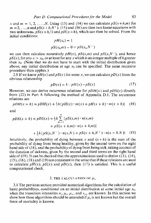
Part D: Computational Procedures for the Model 83
X and m = 1, 2, . . . ,N. Using (13) and (14) we can calculatepS(x+h,m) for m =2 , . . . ,n andpS(x+h,N+). (15) and (16) are then two linear equations with two unknowns, pS(x+ h, l ) and pH(x+ h), which can then be solved. From the initial conditions:
pH(.i,) = l
pS(.r,,m) = 0 = pS(xo,N+)
we can then calculate recursively pH(x), pS(x,m) and pS(x,N+), and hence pS(x), for any x > xo. or at least for any x which is an integer multiple of h greater than X,,. (Note that we do not have to start with the initial distribution given above; any initial distribution at age xa can be specified. The same recursive procedure then applies.)
2.8 If we know pH(x) andpS(.i) for some x, we can calculatepD(x) from the obvious relationship
p ~ ( x ) = I pH(x ) -pS ( . i ) (17)
However, we can derive recurrence relations for pDH(x) and pDS(x) directly from (22) in Part A following the method of Appendix D.1. The recurrence relations are
pDH(x + h) epDH(.x) + $ h ( p ~ ( x ) .m(x) +pH(x + h) .m(x + h)} (18)
and ,v
~ D S ( X + h) pDS(x) + f h 1 (pS(x.m). &m) m = /
+ pS(x + h,m). n(x + h,m)J
+ f h (pS (x ,N t ) . n(x,hr) + p S ( s + h . N + ) . n(x + h,lV)) (19)
Intuitively, the probability of dying between x and ( x f h ) is the sum of the probability of dying from being healthy, given by the second term on the right hand side of (18). and the probability of dyingfrom being sick, taking account of the duration of sickness, given by the second and third terms on the right hand side of (19). It can bechecked that the approximations used to derive (13), (14). (l 5). (16), (18)and (19)areconsistent in the sense that if these relations areused to calculate pH(x), pS(x) and pD(x), then (17) is satisfied. This is a useful computational check.
3. THE CALCULATION OF F.,
3.1 The previous section provided numerical algorithms for the calculation of basic probabilities, conditional on an initial distribution at some initial age X",
when the transition intensities u,.px, p , ; and v,, are known. In this section we show how these algorithms should be amended if p, is not known but the overall force of mortality is known.

84 The Analysis of Permanent Health Insurance Data
3.2 We shall assume throughout this section that ax, p,,z and v,., are known and that the individual was healthy at the initial age xo. This individual's overall, or total, force of mortality a t age xO+ l, denoted pLrml+, is defined by
which shows that the overall force of mortality is a weighted average of pro+,,; and v,.+,.z with weights equal to the probabilities of being healthy or being sick with - duration z at age .q+ t .
3.3 In the spirit of the notation introduced in 92 for the basic transition intensities, we make the following notational definitions:
So that mS(x) represents theaverage force ofmortality among the sick, weighted by duration. Note that both mL(x) and mS(x) are conditional on the individual being healthy at age xo. The following approximate formulae can then be derived:
3.4 It is convenient to definepL(x) to be the probability that the individual is alive at age x, whether healthy or sick, given that he was alive and healthy at the initial age xo. Hence,
PL (X) = P H ~ ) + P W ) (26)
Next we note that the following approximate relationship holds
~ L ( x + h) . z p L ( x ) [ l ~ h . m L ( x ) l i [ I + t h . m L ( X + h)] (27)
(See Waters and Wilkie (1987, formula (IOA)).) Let us suppose now that for some age xo + l , where I is an integer multiple of the
step size h, we know the values of
pS(xo+t,N+) and m ( x ~ + t ) , as well as the values of the other transition

Part D: Computational Procedures for the Model 85
intensities. Then we can calculate
PS(.\+ t + h , m ) m = 2 , 3 ...., N,andpS(x,,+ t + h , N + )
using (13) and (14). We can calculate pL (X, + r + h) from (27). Adding formulae (18) and (19). and noting that
p D H ( x o + t + h ) + p D S ( x o + t + h ) = l - p L ( % + t + h ) (28)
gives us, together with formulae (15) and (16), three linear equations in three unknowns,pH(xo + t + h), pS(xo + t + h,l) and m(x + t + h), which can then be solved. This recursive procedure starts at age X,, where
Hence we can calculate recursively m(% + h), mixo + 2h), etc. It should be noted that the value of m(x) calculated in this way might not be positive; for m(x) to be positive we must assume an overall force of mortality which is consistent with the graduated values of U,, p , , and v ,,,.
4. THE CONSTRUCTION OF AN INCREMENT-DECREMENT TABLE
4.1 The basic probabilities for a simple life table can be conveniently summarized, usually at integral ages, by columns of I,, the number alive at age x out of a given number (the radix) alive at some initial age, and of d,, the number dying between ages X and X + l . A corresponding summary can be constructed for the model for PHI discussed in this Report, although the resulting table, an increment-decrement table, is somewhat more complex than the usual life table.
4.2 We start with a radix, R, at some initial age xo. R represents a (large) number of Lives aged xa with some specified initial distribution of healthy lives and sick lives, with specific durations of sickness. In all our illustrations in Part E we shall assume that all lives are healthy at age xo, although this assumption is not necessary. We make the following definitions for age x xo:
1H(x) the number healthy at age x (= R.pH(x)) iS(x) the number sick at age x: at all durations combined (=R.pS(x)) lDH(x) the number dead at age X, having died as healthy (=R.pDH(x)) lDS(x) the number dead at age X. having died as sick (=R.pDS(x)), IL(x) the number alive at age x (= lH(x) + IS(x)) ID(x) the number dead at age x (= IDH(x) + IDS(x))
(Note that for convenience we refer to lH(x), for example, as the number healthy

86 The Ana1.ysi.s of Permanent Health Insurance Data
a t age x rather than as theexpected number healthy at age X. Thus in this section we could be said to be taking a deterministic, rather than stochastic, view of the model. Note also that to emphasise the analogy with a simple life table, we shall sometimes denote lL(x) by l, in the remainder of this Report.)
4.3 The quantities defined below correspond to d, for a simple life table. dHS(x) the number of transitions from healthv to sick between ages x and X+ l ., d.SH(.x) the number of transitions from sick tdhealthy between ages x and X + 1 dHD(x) the number of transitions from healthy to dead between ages X and X + 1 dSD(x) the number of transitions from sick to dead between ages x and X + 1.
4.4 The quantities defined in the previous paragraph can be calculated as follows:
h - ' - l
RC jh [pH(x+ jh) . s ( x + jh) + p H @ + (;+ I)h).s(x + ( j + 1)h)l (30) 1-0
+pS(x + ( j + l)h,m). r(.x + ( j + I)h,m)) h - # - l
+ RI j h { ~ S ( ( x + j h ) , N + ) . r (x + jh,N) j = "
+pS(x + ( j + I )h ,N+) . r(x + ( j + l)h,N)) (31) h - l i
dHD(x) RC + h { ~ H ( x + jh) .m(x +/h) 1-0
+ pH(x + ( j + I)h) . m(x + ( j + 1)h j (32) h ' - 1 X
dSD(x) RC 411 1 {pS(.x + jh,m). n(x + jh,m) , = O m = ,
Note that (30) and (3 1 )represent the sum over the steps of age x - X + h, X+ h +
x+2h, . . . , X + 1 -h + X + 1 of the number of relevant transitions (multiplied by

Part D: Computational Procedures for the Model 87
R) as given by the right hand side of (15). Formulae (32) and (33)can be derived similarly using (18) and (19) respectively.
5. CLAIM INCEPTION RATES
5.1 In this section we show how we can calculate a claim inception rate. The reader should note that claim inception rates can be defined in a variety of similar, hut not identical, ways. In this section we discuss only two of these ways. Throughout this section we assume that we start with R individuals at age so, all of whom are then healthy.
5.2 We define the following function, L,, which is analogous to the corresponding function for a simple life table.
so that L, represents the (expected) number of years lived between ages x and x + l by the R individuals who were healthy at age xo. We could also interpret L, as the average number of individuals alive between ages x and x + l . We can calculate L, as follows:
5.3 Next we define a function ca(x,d). which represents the (expected) number of claim inceptions between ages x and X + 1 for a given deferred period d. For any step size h we can write
h ' - 1
ca(x,d) = C E [number of claim inceptions between ages (S + jh) and 0
(X + (j + I )h ) l R individuals were healthy at age X,] (36)
For a value of h less than the deferred period d, an individual can have at most one claim inception between ages (x+jh) and (X+ ( j + l )h). Hence (36) can be written
h - ' - ,
ca(.r,d) = RC P [a claim inception between ages (S + jh) and 0
(S + (J + l)h) l the individual was healthy at age .r, ] (37)

88 The Analvsis of Permanent Healrh Insurance Data
We can calculate ca(x,d) from formula (37), at least approximately. as follows
In the special case where the deferred period d is zero (which is useful for illustrative if not for practical purposes) we can still regard (38) as a reasonable approximation to ca(x,O) provided the step size h is sufficiently small for the probability of two or more sicknesses starting within a time interval of length h to be negligible. In this case it would also be possible to use (30) to approximate ca(x_0) since ca(x,O) is equivalent to dHS(x). Note that (38) is (R times) the probability that an individual is sick at exact age (X+ ( j + l )h) with duration of sickness between dand d + h plus an approximation to the probability ofdying or recovering between ages (x+jh) and (X+ ( j + I )h) and between durations dand d+h. (See formula (15).)
5.4 We denote by ia(x,d) the claim inception rate at age x for deferred period d defined as follows
ia(x,d) = ca(x,d)!L, (39)
Note that ia(x,d) is, in probabilistic terms, the ratio of two expected values: the expected number of claim inceptions between ages X and X + 1 for deferred period dand the expected number of years lived between these ages, in both cases out of R individuals who were healthy at some initial age xo. Note that the value of the radix R affects the numerical values of ca(x,d) and L,, but not of ia(x,d), and that the initial condition that all individuals were healthy at age xo affects the values of all three functions. The dependence of ia(x,d) on the initial condition that all individuals were healthy at age xo is not explicit in the notation. For some purposesit isconvenient to make this dependence explicit in the notation and for this reason we define ia(x,d,t) to be the same as ia(x,d) with t denoting the duration since the lives were 'select', i.e. I =S-xu.
5.5 We shall refer to ia(x.d) as a 'type (a) inception rate'. We can define a 'type (b) inception rate' as follows. For any age x and deferred period d we define cbix,d) by
cb(x.d) = ca(x + d,d) (40)
so that cb(x,d) represents the (expected) number of claim inceptions between ages (x+d) and (x+d+ 1 ) out of R individuals who were healthy at age xu. We can interpret cb(x,d) as the (expected) number of sickness inceptions between ages X and (X+ l )which will eventually give rise to claims (between ages (x+d) and (X+ 1 + d)) out of R individuals who were healthy at age xo. We can calculate

Part D: Computational Proceduresfor the Model 89
cb(x,d) using formula ( 3 8 ) with ( x + d ) replacing X. We can also approximate cb(x,d) by
ch(x ,d ) z ( I - r l ) . c a ( x , d ) + d . c u ( x + 1,d) (41
We define our second claim inception rate, ih(x,d), as follows
i b (x ,d ) = cb(x,d ) / L , (42
Note that ih(x,d)is not equal to ia(x+d,d) but, using (40), and (41). we have the following approximation
i b (x .d ) z [ ( l - d ) . L; ia (x ,d ) + d . L,+, . i a ( x + l . d ) ] i L , (43)
6 . MANCHESTER-UNITY-TYPE STCENESS RATES
6.1 In this section we show how we can define and calculate Manchester-Unity- type sickness rates using the basic probabilities for the model. We start by introducing some notation which will be very convenient in this section. For X > xo and numbers a and b, which must be non-negative integer multiples of the step size h, we define
so that pS(s ,a/b) is the probability of being sick at exact age x with duration of sickness between a and <a+ b ) , conditionacas always on be& healthy at age no. Next we introduce the function [ (x ,a!b) which is defined by
so that i (x ,a!b) represents (52 times) the probability that an individual is sick at age x with duration of sickness between a and (a+ h ) , given that the individual is alive at age X and was healthy at some earlier age .Q.
6.2 Finally in this section we define the function z (x ,a /b ) as follows
which, using (34) , can be written

90 The Analysis uf Permanent Health Insurance Data
The numerator of (47) can be calculated using numerical integration as follows
The denominator of (47) can he calculated using (35). The numerator of (47) can be interpreted as the expected number of weeks of sickness between durations a and a + b between ages x and X+ 1 for a group of R individuals who were healthy at age xo; the denominator represents the expected man-years lived between ages x and X+ 1 by these individuals. It can be seen that z (x ,a /b ) is very similar in definition to the central rate of sickness z",:, the important difference being that both the numerator and denominator of z (x ,a /b ) are conditional on an initial status at some earlier age xo.
7 . THE E X A C T CALCULATION OF M O N E T A R Y FCNCTIONS
7.1 In this section we consider the evaluation of monetary functions which are useful for the calculation of premiums and reserves for PHI business. In particular we consider the evaluation of annuities payable while the individual has a given status; for example, sick, with duration between a and ( a + h ) . The formulae given in this section for the evaluation of these annuities are based on the probabilities whose evaluation is outlined in $2 of this Part. Numerical illustrations of these formulae will be given in Part F. Also given in Part F will be alternative, approximate, formulae for the evaluation of these annuities.
7.2 In this paragraph we consider continuous annuities payable in a particular status. All the annuities in this paragraph are the expected present values of annuities of I p.a. payable continuously for a maximum of n years to an individual who is currently healthy at age xo. These annuities are payable only when the individual is in a given status. The notation for these annuities is as follows:
i{L, which is payable only if the individual is alive,
2 which is payable only if the individual is healthy.
iF, which is payable only if the individual is sick. iaTTb' which is payable only if the individual is sick; with duration of sickness
between a and (a + h).
Formulae for these annuities are as follows:

Part D: Conzputational Proceduresfor the Model 9 1
where L = ( l + i ) ' and i is the rate of interest. We can evaluate these annuities. a t least approximately, using the repeated trapezium rule with step size h, together with the algorithms in 92 above. The relevant formulae are:
7.3 In this paragraph we consider a 'current claim' annuity, which we denote p
ss , . This annuity is the expected present value of an annuity of 1 p.a. payable continuously for a maximum of n years to an individual who is currently aged X
and sick, with duration of sickness z. The annuity ceases at age ( n t n ) . or on recovery or on death, whichever occurs soonest. The integral formula for this annuity is:
where (59) follows from formula (27) in Part A.

92 The Anulysi.~ of Permanenr Heulrh Insurance Data
7.4 Now consider an annuity similar tot?:.:,, but payable monthlv i_n advance rathe1 than continuously. We denote the value of this annuity ii,'.L2:y. Hence, a!.!?ydenotes the value of an annuity of 1 p.a. payable monthly in advance (so that the first payment is payable immediate1y)for at most n years toanindividual who is currently aged x and sick, with duration of sickness z. The annuity ceases at age (x+n), or on recovery or on death, whichever occurs soonest. The formula for this annuity is
which can be used to evaluate i i i ~ p w i t h the help of (the approximate j formula (59) .
7.5 In this paragraph we consider annuities payable monthly in advance corresponding to the continuous annuities discussed in $7.2. Formulae for these annuities are as follows:
Note that in each case the payment of 1/12 is made at time ri12 if and only if the individual is in the specified status at that time.

Part D: Computational Procedures for the Model 93
7.6 Finally in this section we consider an annuity which is rather less
1 p.a., up to age ( x ~ + n ) , counting only those claims for which the sickness started hetween ages (xo+ml) and (no+mz) where ml <m?<n. (In practice, particularly for group PHI, we may be interested in the case where ml = 0 and m2 = 1.) The value of this annuity can be written:
(Recall that ddenotes thedeferred period for the policy.) Intuitively, (69) can he explained as follows: y is the age at which a sickness leading to a claim starts (the possible values ofy are xo + ml $ y $ (no + m2) and t is the time after agey when a payment is made (the possible values o f t are d $ r $ xo + n - y ). (Note that, as with the annuities in 557.2 and 7.5, the annuity valued by (69) may include several disjoint periods, corresponding to different bouts of sickness, when the annuity is payable. This is not the case for the 'current claim' annuities considered in 557.3 and 7.4.). The payments valued in formula (69) can he valued by adifferentmethod,separatingthosepaymentsmadehetweenages (xa +m, + d) and (xo + m2 + d) from thosemade between ages (xo + m2 + d) and (xo + n). Consider the following two values:
and
Formula (71) gives the value of a continuous annuity at the rate of 1 p.a. payable from ages (xo + m, + d) to (no + mz + d) if an individual now aged xo and healthy is sick with duration of sickness between dand ( y - xo - ml). Formula (72) gives the value of payments hetween ages (xo + m2 + d) and (,Q + n), where payments are made only if the duration of sickness is hetween (y -xo - m*) and (y -no - ml). It can be seen intuitively that (69) equals the sum of (71) and (72). The algebraic proof of this is included as Appendix D2. These annuities are not illustrated numerically in Part F and hence we have not given formulae in terms of pH( ),PS( ) etc. corresponding to (69), (71) and (72).

94 The Analysis of Permanent Health Insurance Data
APPENDIX D I
In this Appendix we give details of the derivation of (9); the derivations of the other recurrence relations in $2 are similar.
From the definition o f p S ( x + h,m+ I) and formula (28) in Part A, we have
provided X-xo>mh. It is implicit in $2 that (.xPxo) is an integer multiple of h and, if X-xo<mh there is nothing to prove since both pS(x,m) and pS(x+h,m+ l ) are zero. Using formula (27) in Part A, the right hand side of (73) can be written
rnh h - HH . S - P fix-,. , ~ ~ ~ ~ { e x ~ [ - ~ ( p , + . , , + . + v,+.,+.)du] - l } dt (74)
(m - ,)h U
and using the mean value theorem for integrals and formula (28) in Part A, (74) is equivalent to
for some t between (m- l ) h and mh. The mean value theorem for derivatives applied to the first term in (75) shows that (75) is equivalent to
for some f between 0 and h. Formula (76) is an exact expression for (pS(x+h,m+l)-pS(x,m)); to obtain an approximation we first take the average of (76) with f = 0 and f = h as follows:
pS(x + h,m + l ) -pS(x ,m) 2 [-kh{p,,+ v , , ) - k h { ~ , + ~ , + , + v,+r,,,+~}
e x p { - ~ ( P , + , , + . + v ,+, ,+Jdu}l . ~ S ( x , m ) (77) 0
Now note that from the definition o f t
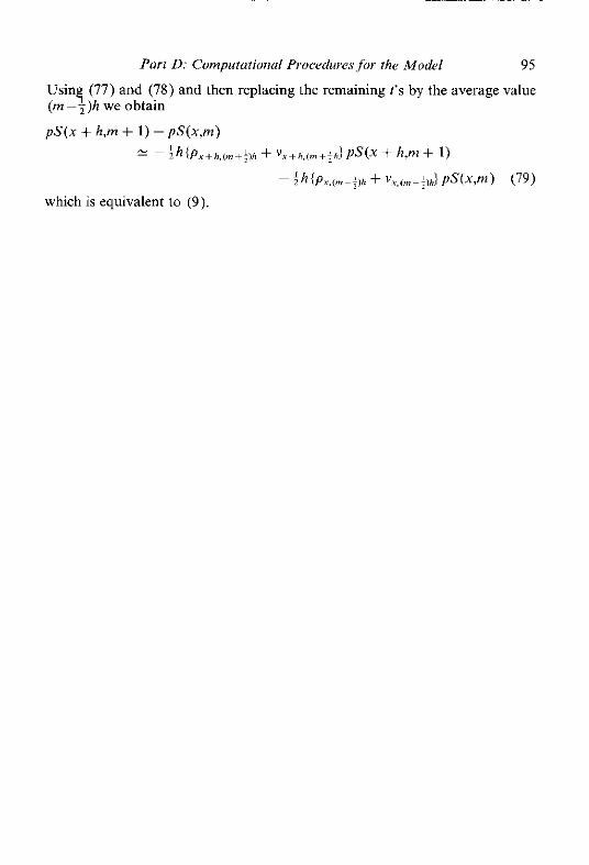
Part D: Computational Procedurrsfor the Model 95
Usin? (77) and (78) and then replacing the remaining t's by the average value (m-?)h we obtain
pS(x + h,m + 1) - pS(x,m)
= - f h { ~ ~ ~ + h , , + j ~ + V ~ + ~ , ~ ~ + ; ~ P S ( ~ + k m + 1)
- ~ h ~ ~ , , , , - ; ) h + % l m jd pS(x,m) (79) which is equivalent to ( 9 ) .

96 The Analysis of Permanenl Health Insurance Data
APPENDIX D2
In this Appendix we show that formula (69) is the sum of formulae (71) and (72). First we note the general result that for any (reasonably well behaved) function, f(z,j>), X0 + m 2 % + "
S f (2,s) dv dz = *,+m, ; + d
This result can most easily he proved by drawing a picture of the (z,y)-plane and noting the area over which integration takes place in each of the three integrals. Next we note that for W G t
This formula follows, by a change of variable, from formula (28) in Part A. Using (8 1 ), formulae (71 ) and (72) become
and
With the change of variable z = t+y in the inner integral, (69) becomes
Changing the notation in (84). i.e. writing y in place of z and i in place of y, we can see that, using the general result (SO), (84) is the sum of (82) and (83).

CMIR 12 (1991) 97-226
PART E: CALCULATION O F PROBABILITIES
SUMMARY
In this Part the rates (transition intensities) which have heen derived in Parts B and C are applied to the model whose mathematical formulation was defined in Part A, using the numerical methods described in Part D.
A further element of the basis, the mortality rates of the healthy, is discussed in Section I. In Section 2 a graphical representation of the sickness model is presented, which may he a useful aid to understanding the model. In Sections 3 to 6 probabilities and rates are derived on one basis, that for a one-week deferred period. The construction of 'select' tables for different rates is discussed in Sections 7 to9. A further useful probability, that of survival while sick during the deferred period, is introduced in Section 10. Results using the bases for other deferred periods are considered in Sectlon I I .
1. MORTALITY OF THE HEALTHY
1 . l A necessary element of the fundamental basis for the calculation of PHI values is the mortality of the healthy, the function px as defined in Part A. The PHI Sub-Committee has no direct information about the mortality rates experienced under PHI policies among those who are not making a claim, which include both the healthy and those who are sick hut with a duration of sick- ness less than the deferred period. It is doubtful whether offices have com- prehensive information on this point; sometimes they may be notified about the death of a policyholder; on other occasions a policy may apparently lapse because of the death of the policyholder but without the office being notified of the death.
1.2 The mortality of those who are sick with a duration less than the deferred period, v,<,, has heen extrapolated from the graduated mortality rates for the sick about whom information is known, as descrihed in Part B. It is, however, necessary to make a plausible assumption about the level of mortality that might be experienced by healthy lives. The mortality assumed For the calculations in this Part is that of Male Permanent Assurances 1979-82, duration 0, as graduated by the GM(2.2) formula shown in the report "The Graduation of the 1979-82 Experience" in C.M.I.R. 9.
97

98 The Analysis of Permanent Health Insurance Data
The formula used was: p,=ao+a~t+exp(b~+b,t j (1)
where t = (X-70) 50 '
an = - 0.00465 192 a l = -0.00452546 bo= -3,985723 h , = +3.185063
A justification for using the duration 0 rates is that they apply to a group of assured lives who had been recently selected, either by medical examination or by medical questionnaire, and who therefore may be expected to have been healthy, or at least not suffering from long-term disability though they might have been currently temporarily sick. These rates are therefore potentially appropriate to represent the mortality of the healthy in a PHI model.
l .3 The rates for the data described as being for 'duration 0' apply to policies in the first year of insurance. and are therefore not strictly those at exact duration zero. If the 'duration 0' graduated rates were treated as applying at exact duration t and the 'duration 1' rates at exact duration l;, then a hypothetical exact duration 0 rate could be obtained by linear extrapolation: l .5 (duration 0)- 0.5 (duration 1). Mortality rates so calculated for 1979-82 Male Permanent Assurances were used in one of the experiments carried out to investigate the sensitivity of the results to alternative assumptions about the mortality of healthy lives.
An extreme choice for p, was to assume that the mortality of healthy lives was zero throughout.
Investigations using different assumptions for p, showed that the calculated results were in general fairly insensitive to the assumptions made about the mortality of the healthy, so it wasdeemed most convenient to use the 'duration 0' rates described above.
2. G R A P H I C A L REPRESENTATION
2.1 For clarification of some of the factors discussed below it may he convenient to use a graphical representation of the development of sickness. Figure El shows such a graphical representation of the model for sickness. Imagine that a group of healthy lives aged xo starts at point A in the diagram. So long as they remain healthy they travel down the heavy vertical line, their age increasing as they go.
Various alternative paths are depicted in the diagram. At point B, for example, one life might become sick. The duration of sickness is represented by the horizontal axis to the right of the heavy vertical. Lines representing 13 weeks and 26 weeks sickness are shown. As time passes both the age and the duration of sickness increase simultaneously. This is represented by assuming that our

Dead from
Healthy
Parr E: Calculation of Probabilities 99
Healthy Sick Dead from
A -c Duration of sickness Sick X, *---------
Figure E l . Model of sickness
specimen life travels down the diagonal line from B towards C, atwhich point he recovers and moves immediately back to the healthy state at point D. It can be seen that on this occasion he was sick for rather longer than 13 weeks but less than 26 weeks, and would therefore have had a potential claim under a 13-week deferred policy, but not under a 26-week deferred one.
At point E another healthy life (or the same again) becomes sick. Hecontinues down the diagonal line, beyond the 26 week line to point F, at which time he dies. This is represented by the line from F to G. The heavy vertical line to the right of the diagram represents the path of those who died while in the status sick.
Another example becomes sick at point H, continues to I and recovers to J. He is sick for less than 13 weeks, and could not claim under a 13-week deferred policy.
Another example dies while in the healthy state at point K, moving across to L in the vertical line to the left of thediagram. which represents those who die in the healthy state.
Yet other examples become sick at points M, 0 and Q. They are all still sick at the end of the period under consideration which is represented by the horizontal
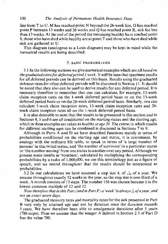
100 The Analysis of Permanent Health Insurance Data
line from T to U. M has reached point N beyond the 26-week line, 0 has reached point P between 13 weeks and 26 weeks and Q has reached point R, sick for less ihan 13 weeks. At the end of the period the remaining health; have reached point S, those who have died while healthy are at point Tand those who have died while sick are gathered at U.
This diagram (analogous to a Lexis diagram) may be kept in mind while the numerical results are being described.
3. BASIC PROBABILITIES
3.1 In the following sections we give numerical examples which are all basedon thegraduatedrates for deferredperiod I week. It will be seen that specimen results for all deferred periods can be derived on this basis. Results using the graduated sickness rates for other deferred periods will be discussed in Section 11. It should be noted that they also can be used to derive results for any deferred period. It is necessary therefore to remember that one can calculate; for example, 13-week claim inception rates on the l-week deferred period basis or on the 13-week deferred period basis or on the 26-week deferred period basis. Similarly, one can calculate l-week claim inception rates, 13-week claim inception rates and 26- week claim inception rates all on the l-week deferred period basis.
It is also desirable to note that the results to be presented in this section and in Sections 4, 5 and 6 are all conditional on the starting status and the starting age, which in these examples are taken as healthy at age 30. Theextent to which results for different starting ages can be combined is discussed in Sections 7 to 9.
Although in Parts A and D we have described functions mainly in terms of probabilities conditional on the starting age and status, it is convenient, by analogy with the ordinary life table, to speak in terms of 'a large number of persons' in this initial status, and 'the number of survivors' in a particular status or 'the number moving' from one status to another over any period. Although we present some results in 'numbers', calculated by multiplying the corresponding probabilities by a radix of 1,000,000, we use this terminology just as a figure of speech, and we intend throughout that the results should be interpreted as probabilities.
3.2 In our calculations we have assumed a step size h, of of a year. We assume throughout exactly 52 weeks in the year, so the step size is one-third of a week. A month consists of 13 steps. The number 156 was chosen because it is the lowest common multiple of 12 and 52.
Note therefore that in this Part (andin Part F) a 'week'isalways& of a year. and not an exact seven days.
The graduated recovery rates and mortality rates for the sick presented in Part B vary only by attained age and not by duration once the duration exceeds 5 years. We have therefore been able to amalgamate durations after 5 years (780 steps). Thus we assume that the integer N defined in Section 2.3 of Part D has the value 780.

Part E: Calculation of Probabilities 101
3.3 The basis used has already been stated as that relating to deferred period 1 week. To be precise it is:
Mortality of the healthy, fix: Male Permanent Assurances 1979-82 duration 0 graduated rates, as described in Section 1 above.
Sickness inception rates, ex: the graduated rates for deferred period 1 week as given by formula (9) in Section 9.1 of Part C.
Recovery rates, p,:: the graduated rates for deferred period I week, as given by formula (6) in Section 4.4 of Part B.
Mortality rates of the sick, v,,;: the graduated rates for all deferred periods as given by formula (9) in Section 6.2 of Part B.
3.4 The basic probabilities are given in Table E14, which is expressed in terms of 'numbers' based on a radix of 1,000,000 (=R) as described in Section 4.2 of Part D. The columns towards the left show the numbers in each status at each integral age from 30 to 65. These are analogous to the 1, column of a life table, and they have been denoted:
IH(x) the number of healthy = R.pH(x), lS(x) the number sick (at all durations combined) = R.pS(x), lDH(x) the number dead, having died as healthy =R.pDH(x), IDS(x) the number who have died as sick = R.pDS(x), /L@) the number living= IH(x)+ lS(x) = R.pL(x), ID(x) the number dead = lDH(x) + lDS(x) = R.pD(x).
The number living plus the number dead in every case exhausts the statuses, and the sum of these columns is always equal to the radix R.
The columns towards the right of Table E14 show the numbers of transitions taking place between ages X and X + 1. They are analogous to the number of deaths, d,, in a life table and they have been denoted:
dHS(x) the number of transitions from healthy to sick between ages x and X + l ,
dHD(x) the number of transitions from healthy to dead between ages X and x + l ,
dSH(x) the number of transitions from sick to healthy, i.e. recoveries, between ages x and X + 1,
dSD(x) the number of deaths among the sick between ages x and X + 1.
It can be seen that certain accounting identities hold, for example:
IH(x + l) = IH(x) p dHS(x) - dHD(x) + dSH(x) (2) and
/S(x + 1) = /S(x) + dHS(x) - dSH(x) - dSD(x), (3)

102 The Analvsis o]Permanent Health Insurance Datu
and these are confirmed numerically (subject possibly to rounding errors, since
transitions from healthy to sick between ages X and x + l for a person who commenced healthy at age 30, and similar interpretations apply to dHD(x). dSH(x) and dSD(.u).
3.5 It can he seen that by age 65 about 69% of those starting healthy at age 30 are in the healthy state, and about 13% in the sick state. About 8.3% have died while in the status healthy and 9.6% have died while sick. On this basis rather more die each year while sick than while healthy. but this result is specific to this basis, as can be seen from Table E10 in which the results on different bases are compared.
3.6 i t should be noted that the method of numerical calculation adopted requires the probabilities shown for integral ages in Table E14 to becalculated at steps of & o f a year; thus the table shows only every 156th entry in the full table available inside the computer.
3.7 Besides calculating probabilities at every A t h of a year of age, it is necessary to calculate the proportion sick within each step of &h of a year of duration of sickness up to 780 steps (5 years) in all, with all sickness periods beyond that duration aggregated. It is convenient to print out only the proportion sick for selected sickness periods. as shown in Table E 15. This shows the proportions sick at each age from 30 to 65 within the sickness periods shown, denoted in the usual 'aib' notation. For example, '4/9 weeks' indicates those who have been sick for at least 4 weeks but not more than 4+9= 13 weeks. Wedenote
decimal fractions, not multiplied by the radix R. The iast two columns show the 'Total' sick, equivalent to 'OiAll', and also 'l/All'. The total figure, if multiplied by the radix of 1,000,000, is identical with the number sick, IS(x) of Table E14.
3.8 In Table E16 the functions are shown. These weredefined in Section 6.1 of Part D as 52 times the proportion sick within a specific sickness period among the total living at age X (all conditional on the initial status at age xo). The formula is therefore:
The rates will be referred to again when sickness rates are discussed in Section 6.
4. AGGREGATE MORTALITY RATES
4.1 In Section 3 of Part D it was shown how the overall force of mortality at age X, conditional on the initial status at age xo, could be calculated. The total force of

Part E: Calculation of Probabilities 103
mortality of the living, mL(x), can be considered as the weighted average of the mortality of the healthy and the mortality of the sick. The force of mortality of the healthy is simply p,(=m(x)), and this applies at age X to the proportion healthy at age X, pH(x). The average force of mortality of the sick, weighted by duration, is defined as mS(x) and it can he calculated by the approximate formula (formula (24) of Part D)
The total force of mortality of the living, mL(x), is then calculated by the formula
which is the same as formula (25) of Part D. 4.2 The values of pr, mS(x) and mL(.v) are given in the first three columns of
Table E17. It can be seen how, on the basis used, the value of mS(x), which is undefined at the starting age of 30, is comparatively constant thereafter, rising only from about 0.061 at age 3 1 to 0.082 at age 65. The values of mL(x), however, rise in line with the values of px, and, on this basis, are generally rather more than twice the value of p,.
A comparison of the values of mL(.r) with the values of p.v for durations 2 and over for Male Permanent Assurances 1979-82 (AM80 ultimate) is shown in Table El . After one year the values of mL(s) (on this basis) are substantially higher than the values of p, for permanent assurances, the ratio reducing with age. (For a comparison on the bases for other deferred periods see Section 11.)
It can be seen from Table E17 that the values of mS(.r) exceed the values of mL(x) or of p, on AM80 ultimate by about 0.06 to 0.07.
4.3 The values previously shown for the total living, lL(x), allow the calculation of a total life table, including both the healthy and the sick. Values of
Table El . Comparison of ouerall mortality rates
AM80 ultimate
0.000557 0.000666 0-001077 0-001961 0.W3598 0-006435 0.011184 0.018978
Difference Ratio "4
0.000429 177 0000SSO 182 0.000672 162 0.000759 139 0-000787 122 0.000779 112 0.000939 108 0.001997 I l l

104 The Analysis of Permanent Heulth Insurance Data
lX and q, for this life table are shown in further columns of Table E17. The values of l, are the same as lL(x) in Table E14. The values of q, are calculated in the usual way as
The values can equivalently be calculated by the formula
The average number of living between ages X and X + l is given by the integral
and this has been calculated approximately by
as described in Section 5.2 of Part D. Values of L, are also shown in Table El 7. Over the age range shown the simple
approximation
reproduces the more accurate approximation shown above to within two parts in 10,000, which is probably negligible for practical purposes.
5. CLAIM INCEPTION RATES
5.1 The calculation of claim inception rates on two different definitions was Jcscrihcd in Scitiun 5 o i P ~ r t I). \'alucsoiboth t!pesok'slaim inzeprion ralcson the \peciinen h.r\i\arc > h ~ u n inTilhlc~ EIXa dnd E l n b The) dredenored I ~ . Y . ~ / )
:and ,h( Y.J ) , :irccondition;il on the hie hang hcalthy .it i g c r ,.and drcdetind as:
(a) the expected number of periods of sickness which pass through duration d between attained ages X and X + l (sickness being commenced between ages x - d and X + l - d ) , denoted by ca(x,d), divided by the average number living between ages X and X + l , L,; and
(h) the expected number of periods of sickness which pass through duration d

Parr E: Calculation of Probabilities 105
between attained ages x + d and x + d + 1 (sickness having commenced between ages X and X + I ) , denoted by cb(x,d), also divided by h.
The values shown in Tables El8a and El8b are 10,00Oia(x,d) and 10,00Oib(x,d), and the value of 1 0 , 0 0 0 ~ ~ ~ at exact age X is shown for comparison.
It can be seen from Tables E18a and E18b that the claim inception rates for deferred period 0 weeks, which are the same in both tables, are smaller than the value of a, by an increasing amount as age increases. This is because the sickness inception intensity applies only to the healthy lives, whereas the claim inception rates that we have defined are applied both to the healthy and to the sick. However, the rates are of the same order of size, whereas the claim inception rates for higher durations (dgreater than 0) reduce in value very rapidly as duration increases.
A healthy life aged 30 cannot reach duration of sickness 52 weeks within the first year, nor 104 weeks within the first two years. The claim inception rates of type (a), in the top right hand corner of Table E18a, for 52 weeks deferred at age 30 and 104 weeks deferred at ages 30 and 31 are therefore necessarily zero. This is not the case for the claim inception rates of type (b).
5.2 A graphical representation of the claim inception rates that we have defined is shown in Figure E2. A group of healthy lives commenced at age .Q at point A. Those who are healthy at age X appear at point B, and those who are healthy at age X + l are at point C. The line AEFG represents the course of a person who became sick immediately at age .Q and has remained sick ever since. It forms the boundary of the area within which sickness can occur for this group of lives, so that no sickness can appear above and to the right of this line.
The average number living between ages X and X + l , L,, is represented by the integral of the healthy over the line BC and the sick over the area BCFE. The end of deferred period dis represented by the vertical line through HIJK. The claim inceptions of type (a), cu(x,d), are those which cross this line between H and J, having commenced sickness between ages X-d and X + l -d. The claim inceptions of type (b) relate to cases which pass the end of deferred period d having commenced their period of sickness between ages X and X + 1, represented by the cases that cross the d line between I and K.
5.3 The claim inception rates of type (a) derived for deferred period I week on the specimen basis (which is the basis for I week deferred business), can be compared with the graduated claim inception rates shown in Table H5 of C.M.I.R. 7, except for those in the first year. A summary comparison is shown in Table E2.
It can be seen that these rates are reasonably similar. A comparison of inception rates for other deferred periods is shown in Table E12.
5.4 Values of ib(x,d) can be calculated by interpolation from values of ia(x,d) using formulae of the type:
ib(x,d) = {(l -d)ia(x,d) . L, + d . ia(x + 1,d). L,+,}/L, (12)

106 The Analysis of Permanent Health Insurance Data
Dead Healthy Sick Dead from from
Healthy Sick -W Duration of sickness r------------
Age
Figure E2. Claim inceptions.
with appropriate modifications for the early years, and where d> l . Extensive experimental calculations showed that this formula is very accurate for years after the first and even in the first year is only inaccurate by about 1.5% at the maximum, for deferred period 26 weeks.
Table E2. Claim inception rates of type (a) per 10.000
Calculated on D1 bass C.M.I .R . 7, Table H5 Age (age 30 at entry) Dp 1 week
31 1,224 1.232 35 1,236 1,255 40 1,249 1.268 45 1,281 1.284

Part E: Calculation of Probabilities 107
6. SICKNESS RATES
6.1 In Section 6 of Part D the formula for calculating Manchester-Unity-type sickness rates, z ? ' ~ or z(x,a/b), was discussed.
Numerical values are shown in Table E19. The values of z(x,u!b) are measured in weeks of sickness (assuming 52 weeks per year) for the usual sickness periods, together with the total for all periods 'O/All' and 'I/All'. It can be seen from Section 6 of Part D that the z rate is derived by integrating the numerator and the denominator of the l rates from ages x to X + 1. Both integrals are approximated by summations using the trapezium rule, as shown above from the calculation of L,, which forms the denominator of these rates.
It may be expected that there might be very little numerical difference between z(x,a/b) and ((x+i,u:'b). It can be seen that, on the specimen basis shown, there is only a small numerical difference between z(x,a/b) and the average of [(x,u/b) and [ ( X + I.a/b). Apart from the first year, for all periods of sickness, and for the first year or two for higher periods of sickness (what we shall call the 'run-in period'-not the same as the 'run-in period' of Part B) the difference is not greater than 3 parts in 1,000.
6.2 The values of ;(x,a/b) calculated on this specimen basis are compared in Table E3 with the graduated rates for deferred period 1 week business shown in Table HI of C.M.I.R. 7.
After the run-in period the ratesshown areat a similar level,except for sickness period 104/all. The rates there diverge as the age increases. It should be remembered that the rates shown in Table E19 apply only to those who are
Table E3. Compurison of sickness rules: Table E19 and Table HI of C.M.I.R. 7
Age Table
30 E19 H I
35 E19 H1
Sickness periods
13\13 26/26
0.016 0.005 0019 0.017
0035 0-028 0.032 0-030
0.051 0.045 0.046 0.046
0.074 0.073 0.063 0.068
0112 0-121 0.089 0.102
0,177 0-209 0.146 0.171
0.296 0.379 0261 0341

108 The Analysis of Permanent Health Insurance Data
known to have been healthy at age 30, whereas the rates shown in C.M.I.R. 7 apply to a population who were healthy at a mixture of different entry ages.
7. CONSTRUCTION OF SELECT TABLES-MORTALITY RATES
7.1 In the preceding sections we have described the functions that can be calculated using the full multiple state model. The functions are, in every case, dependent upon the initial status, in our example healthy at age 30. Similar calculations can be carried out for any age at entry and for any chosen status, either healthy or sick with duration of sickness between jand j+ 1 steps. (It would be possible to consider a life with initial duration of sickness z exactly, but the consequent algorithms and computer programs would require many minor changes throughout to effect this, whereas the same program will work for healthy lives and for those sick within one duration step.) It would also be possible to start with any desired probability distribution of statuses as the initial position, corresponding perhaps to a mixed population with specified properties. It can readily be seen, however, that the volume of calculation and corresponding output of tables in order to present every possibility, or even every possible starting age for the healthy, would be substantial. It is appropriate, therefore, to investigate whether the tables can be summarised in some convenient form, in the same way as 'select' life tables are constructed.
In this section we consider the construction of a select total life table, and in Sections 8 and 9 we consider the construction of select tables for inception rates and for sickness rates. The 'selection' in this case results entirely from the model, in which it is assumed that the life enters in the state 'healthy'. It does not reflect any further medical selection, such as might occur in reality.
7.2 In order to investigate the construction of select tables we adopted the following procedure. We calculated tables similar to those shown in Tables E14 to E19 for each entry age of healthy lives from 16 to 64, though they are not shown in this Report. Commencing the calculations with an entry age of 16 allows suitable 'ultimate' rates to be derived, although great reliance should not be placed on the results for the earliest years of age.
Weconsidered first the values of the aggregate 1 -year mortality rates, g,, which are shown for entry age 30 in Table E17. Putting together the results for all entry ages allowed a large triangular table to be constructed with entry ages from 16 to 64 and attained ages from 16 to 64, containing entries for q(x,t) the value of q, for attained age x for a life who entered at age X- t . It was soon seen, as might be expected, that the values of q(x,t) for any one attained age were very similar after the first few years of duration. We describe the rates for age 16 at entry as 'ultimate' rates (although at attained age 16 the one rate is for entry age 16 duration 0). We calculated the ratio of each 'select' rate to the 'ultimate' rate for the same attained age, i.e.

Part E: Calculation of Probabilities 104
It could be seen that the select rates ran in very quickly to the ultimate rates. The maximum difference was at attained age 64. The ratios the select rates bear to the ultimate rate (whose value is 0.014647) are shown in Table E4a.
By comparison, at attained age 40 the comparable ratios are as shown in Table E4b. The value of the ultimate rate is 0.001831.
Table E4a. Rotio of q~ for entry age shown to q64 for entry age 16
Entry age
M 63 62 61 60
59 58 57 56 55
Duration "10 Ratio 0 71.3 I 87.3 2 91.6 3 9 3 6 4 94.9
5 9 5 8 6 96.6 7 97.2 8 97-7 9 98.1
Table E4b. Ratio of q, for entry age shown to y4o for entry age 16
Entry age Duration "/U Ralio 40 0 86.0 39 1 95.4 38 2 97.0 37 3 97.7 36 4 98.2
35 5 98.5 34 6 98-8 33 7 99.0 32 8 99 2 3 1 9 99.4
7.3 We construct a select table with T years selection as follows:
for select durations
q [ . , l+ , = q(x,r) fo r t = 0 to T- l and X = 16 to 64; (13) for the ultimate rates
q, = q(x,x- 16) fo rx = 16 + T t o 64. (14) The question is what value to use for T. If the view were taken that it was
sufficient to jump straight to the ultimate rate when the select rate approached to

110 The Analysis of Permanent Health Insurance Data
within 10% of the ultimate rate, then a table with 2 years selection would be sufficient. If it were felt that the select period should continue so long as the select rates were at least 5% different from the ultimate rate, then the select period would need to be 5 years.
Another approach is to compare the values of 6s_,p,,l on the select basis and on the exact basis for each age. The error is less than 3 parts in 1,000 for all ages for a 5-year select table (and for ages l6 and 60 to 64 at entry the error is zero) and is less than 5 partsin 1,000 for a 2-year select table. The maximum error for a 5-year select table is 0.23"' for I I P ~ Y J and for a 2-year select table is 0.43% for spls,].
Yet another way of assessing the select period needed is to consider the values of ,qrxl = 1 < p l I . the probability of death within t years of a select life entering at age X. The proportionate error in ,qXl is larger than that in ,plxl. Values of ,q1,1 calculated using a limited-period select table are slightly higher than those calculated for each separate age at entry. The maximum excess for a 5-year select tahle is 1.77% for 9qls61, and for a 2-year select tahle reaches 4.66% for sqlml.
If the select tables were to be used for calculating the value of benefits on death, then the error in the overestimation of deaths for a 2-year select table might be considered significant. However. since the life tahle in the context ofPHI benefits is mainly used for the calculation of premium rates, the error in , p , is the important one, and for this purpose a 2-year select life tahle may be satisfactory. However, because a 5-year select period proves to be preferable for inception rates and sickness rates, as is shown in Sections 8 and 9, we have used a 5-year select period in subsequent calculations.
7.4 Tables E2Oa and E20b show the values of ql,-,l+, for attained age X and select duration t , for a 2-year select period and for a 5-year select period respectively. The ultimate rates in each case are in the columns headed '2 and over' and ' 5 and over'. The rates for select durations 0 and 1 are the same in both tables.
TablesE2laand E21b show the values of li,-,l+i for a 2-year and a 5-year select table respectively, in each case based on a radix of 165= 1,000,000.
I t should be noted that, unlike the select mortality tables sometimes displayed elsewhere, a life entering at select duration 0 runs diagonally down to the right as his attained age and duration since entry increases, until he reaches the ultimate column.
8. CONSTRUCTION OF SELECT TABLES-INCEPTION RATES
8.1 It is intuitively reasonable to assume that the claim inception rates described in Section 6 might. after some suitable run-in period, be similar at any one attained age for different starting ages. Tables comparable to Table E18a showing inception rates of type (a ) for each entry age were calculated. Inspection of these showed that the assumption just described is indeed true. However.
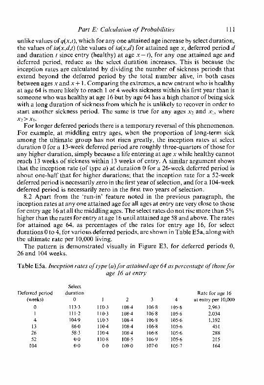
Parr E: Calculation of Probabilities 111
unlike values of q(x.r), which for any one attained age increase by select duration, the values of ia(x,d,t) (the values of ia(.x,d) for attained age X, deferred period d and duration t since entry (healthy) at age X- t), for any one attained age and deferred period, reduce as the select duration increases. This is because the inception rates are calculated by dividing the number of sickness periods that extend beyond the deferred period by the total number alive, in both cases between ages x and X + 1. Comparing the extremes, a new entrant who is healthy at age 64 is more likely to reach 1 or 4 weeks sickness within his first year than is someone who was healthy at age 16 hut by age 64 has a high chance of being sick with a long duration of sickness from which he is unlikely to recover in order to start another sickness period. The same is true for any ages .Q and X,, where X?>X,.
For longer deferred periods there is a temporary reversal of this phenomenon. For example, at middling entry ages, when the proportion of long-term sick among the ultimate group has not risen greatly, the inception rates at select duration 0 for a 13-week deferred period are roughly three-quarters of those for any higher duration, simply because a life entering at age .x while healthy cannot reach 13 weeks of sickness within 13 weeks of entry. A similar argument shows that the inception rate (of type a) at duration 0 for a 26-week deferred period is about one-half that for higher durations; that the inception rate for a 52-week deferred period is necessarily zero in the first year of selection, and for a 104-week deferred period is necessarily zero in the first two years of selection.
8.2 Apart from the 'run-in' feature noted in the previous paragraph, the inception rates at any one attained age for all ages at entry are very close to those for entry age 16 at all the middling ages. The select rates do not rise more than 5% higher than the rates for entry at age l6 until attained age 58 and above. The rates for attained age 64, as percentages of the rates for entry age 16, for select durations 0 to 4, for various deferred periods, are shown in Table E5a, along with the ultimate rate per 10,000 living.
The pattern is demonstrated visually in Figure E3, for deferred periods 0, 26 and 104 weeks.
Table E5a. Inception rates of type (a) for attained age 64 aspercentagr of those for age I6 a t entry
Select Deferred period duration
(weeks) 0
0 113.3 1 11 1.2 4 1049
13 86.0 26 583 52 0.0
104 0-0
Rate [or age 16 3 4 at entry per 10,WO
106-8 105.6 2,963 1068 105-6 2.034 106.8 105-6 1,192 106-8 105.6 451 106.8 105-6 288 1069 105.6 215 107.0 105-7 164

The Analysis of Permanent Health Insurance Data
. . . . . . . . , , . . . . . . , . . . . .. Ourotlon 0 S 1 0 15 20 25 30 35 40 4548 Apeot.ntry 64 59 54 49 44 39 34 29 24 19 16
Figure E3. Inception ratesof type (a) for attainedage 64. A shows theinception rate for entry age 16. B shows the inception rate for duration 5 years.

Part E: Calculation of Probabilities 113
8.3 One approach to constructing select tables for inception rates would be to use the rates for age 16 at entry as the ultimate rates, and to use a select period of, for example, 5 years. We describe this as Method A. However, it may be important that the inception race\ In m y 51.inJ.ird rdhlei are nt>l too loir.1 .An altcrn;~li\s morouch. i r hich we degrihc a t Method B. 1s lo retain sa\ ~ h c lird lit,< . . years of select rates, i.e. those for durations 0 to 4, and then to use the rates for the next select duration, i.e. 5, as if they were the ultimate rates, i.e. to use them for all subsequent durations. Rates for attained age 64 as percentages of the duration 5 rates are shown in Table E5b.
Table E5b. Inception rates of t.vpe (a) for attained age 64 as percentage of those for duration 5
Select Deferred period duration Rate for duration 5
(weeks) 0 l 2 3 4 per 10,000
0 108.4 1055 103.6 102.1 101-0 3,099 I 1063 1055 103.6 102-1 1010 2,128 4 100.3 105.5 1036 102.1 1010 1,247
13 82.2 105.5 1036 102-1 101.0 471 26 55.7 1056 103.6 102.1 101-0 302 52 0 0 106.0 103.7 102-2 101-0 225
104 0.0 0 0 104-1 102.2 lOl.0 171
Method B slightly overestimates the inception rates, and the measure of the aggregate overestimation can be obtained by calculating the total 'number' of inceptions for a life aged X a t entry (in the healthy state) calculated both on the complete table (treating each age at entry independently) and on the select table.
The pattern for type (b) rates is almost the same, except that the 'run-in' feature shown in the lower left hand corner of Tables E5a and E5h does not exist.
8.4 Formally, a select table with T years selection is defined as follows:
for the select durations (Methods A and B) . d za,,-,,+, = ia(x,d,t) for t = 0 to T - 1 and X = l6 to 64; (15)
for the ultimate rates (Method A)
ia,d = ia(x,d,x- 16) (16)
for the ultimate rates (Method B)
ia.; = ia(x,d,T) (17)
Similar formulae would apply to the inception rates of type (h), which could be derived from the inception rates of type (a) by formula (12) of 5.4.
8.5 The inception rate of type (a), ia(x,d), was defined in Section 5 above and in Section 5 of Part D by the formula
ia(x,d) = ca(x,d)/L,. (18)

114 The Analysis of Permanent Health Insurance Data
Given values for iu(x,d) and L, it is therefore possible to reconstruct ca(x,d), the 'number' of claim inceptions starting between ages X and x + 1, conditional on a life commencing as healthy at age no. To emphasise the fact that these rates are conditional on being healthy a t age xo we use the notation:
i a ( x , d , ~ - X) = ca(x,d,xo- x)lL(x,xo). or ia(xo + t,d,r) = ca(xo + t ,d, t) lL(xo + t,xo) (19)
The total number of claim inceptions for deferred period d, for a life who is healthy at age x ~ , within n years can be defined as Tca(xo,d,n) and calculated as
n - l
Tca(xo,d,n) = X ca(xo + t,d,t) I - 0
The equivalent function calculated using select tables can be defined as Tca'(xo,d,n) which can be defined as
where ia and L are both taken from the appropriate select table, with the chosen numbers of years selection. (It is not essential that the same number of years selection be used for the life table and for the inception rate table.) Note that the subscript [xo]+ t is taken as .Q+ t for t > T, the select period for the table.
We can calculate L by
8.6 We have calculated Tca(xo,d,n) and Tca'(xo,d,n) for both Method A and Method B for each entry age from 16 to 64, each termination age from 17 to 65, and for the deferred periods 0,1,4, 13,26,52 and 104 weeks, using a select period of 5 years. We have defined the percentage error as
The maximum errors are as shown in Table E6. It can be seen that the values of Tca' calculated using Method A are at the
worst slightly less than the values of Tca calculated using the full table for each separate entry age, but the maximum error never exceeds 2%. Using Method B the maximum error is in the the other direction, and for most deferred periods is slightly larger, reaching a maximum of more than 2%. Further, the maximum error using Method A occurs only for a rather high entry age, terminating at age 65, and for most ages and terms the percentage error is considerably smaller. By
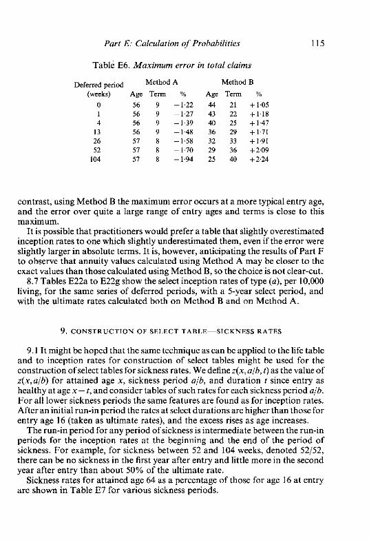
Part E: Calculation of Probabilities
Table E6. Maximum error in total claims
Deferred period A Method B (weeks) Age Term % Age Term %
0 56 9 -1.22 44 21 f l . 0 5 1 56 9 -127 43 22 + l 1 8 4 56 9 -1.39 40 25 + 1.47
13 56 9 -1.48 36 29 +1.71 26 57 8 -1.58 32 33 +1.91 52 57 8 - 170 29 36 f2.09
104 57 8 - 1.94 25 40 f2.24
contrast, using Method B the maximum error occurs at a more typical entry age, and the error over quite a large range of entry ages and terms is close to this maximum.
It is possible that practitioners would prefer a table that slightly overestimated inception rates to one which slightly underestimated them, even if the error were slightly larger in absolute terms. It is, however, anticipating the results of Part F to observe that annuity values calculated using Method A may he closer to the exact values than those calculated using Method B, so the choice is not clear-cut.
8.7 Tables E22a to E22g show the select inception rates of type (a), per 10,000 living, for the same series of deferred periods, with a 5-year select period, and with the ultimate rates calculated both on Method B and on Method A.
9. CONSTRUCTION OF SELECT TABLE-SICKNESS RATES
9.1 It might be hoped that the same technique as can he applied to the life table and to inception rates for construction of select tables might be used for the construction of select tables for sickness rates. Wedefine z(x,a/b, t ) as the value of r (x ,a /b ) for attained age X , sickness period ajb, and duration t since entry as healthy at age X - t , and consider tables of such rates for each sickness period ajb. For all lower sickness periods the same features are found as for inception rates. After an initial run-in~eriod the rates at select durations are higher than those for entry age 16 (taken as ultimate rates), and the excess rises as age increases.
The run-in period for any period of sickness is intermediate between the run-in periods for the inception rates at the beginning and the end of the period of sickness. For example, for sickness between 52 and 104 weeks, denoted 52/52, there can be no sickness in the first year after entry and little more in the second year after entry than about 50% of the ultimate rate.
Sickness rates for attained age 64 as a percentage of those for age 16 at entry are shown in Table E7 for various sickness periods.

1 16 The Analysis of Permanent Health Insurance Data
Tahle E7. Sickness rates for attained age 64 as percentage of those for age 16 at entry
Select Sickness duration period 0 1
0: l 112.3 110-3 l 13 108.3 110.3 419 96.9 110-4
13/13 73.2 110.4 26/26 309 110.6 52/52 0.0 59.2
104/all 0.0 0.0
Sickness rate for age 16 at entry
3 4 (weeks)
1064 105.6 0.239 106-8 105.6 0.473 106.8 105-6 0.621 106.8 105.6 0-454 106.9 105-6 0.632 106.9 105.7 0-970 266 39-8 4.420
The pattern is demonstrated visually in Figure E4, for sickness periods Ojl, 26/26 and 104/all.
Comparison with the percentages shown above for inception rates at attained age 64 shown in Section 8 demonstrates the lengthened run-in period, represented by lower percentages at select duration 0 and in some cases select duration I , followed by ratios which are very similar to those in Tahle E5a. Ratios as percentages of the sickness rates for duration 5 are shown in Table E8.
Tahle E8. Sickness rates for atrainedage64aspercentage of those for duration 5
Select Sickness duration period 0 I 2 3
0; l 107.4 1055 1036 102.1 113 103.5 105.5 103.6 1021 4/9 9 2 7 105.5 103.6 102.1
13/13 70.0 105.5 1036 1021 26/26 26.6 1057 1037 102.1 52/52 0.0 56.6 1038 102-2
104/all not appropriate to calculate
Sickness rate for duration 5
4 (weeks)
101.0 0-251 101-0 0.495 101-0 0-M9 101.0 0.475 101.0 0-662 101-0 1.015
2-236
9.2 Select tables for sickness periods up to 52/52 can therefore be constructed, on the same lines as for inception rates, both on Method A, using the rates for entry age 16 as the ultimate rates, and on Method B, using the rates for select duration 5 as if they were ultimate rates, for the same reasons as described under inception rates. Formally, we put:
for the select durations (Methods A and B) 0ib z, +, = z(x,a/h,t) for t = 0 to T- l and X = l6 to 64;

Part E: Calculation of Probabilities 117
.30,
Sio%. period l 04/.,ll
s , o v L .rlod g/i
.20-
.IS-
.TO-
.OS-
0 ,
Figure E4. Sickness rates for attained age 64. A shows the sickness rate for entry age 16. B shows the sickness rate Car duration 5 years.
B A
1 v- Duration 0 5 10 15 20 2.5 30 35 40 4 5 4 8 APOt.ntry 64 59 54 49 44 39 34 29 24 19 16

118 The Analysis of Permanent Health Insurance Data
for the ultimate rates (Method A)
=:'h - z(x,a/b,x - 16)
for the ultimate rates (Method B)
z,"" = z (x,a/b, T )
9.3 It will, however, be seen from the bottom line in Table E7 or from the lowest diagram in Figure E4, that the select rates for sickness period 104/all do not run into the ultimate rates at all quickly. This is true not just for attained age 64, but for all attained ages. The run-in period lasts indefinitely. For example, no select rate approaches within 5% of the rate for entry age 16 within the first eight years from entry, and at select duration 8 it is only the rate for age 25 attained (age 17 a t entry) that exceeds 95% of the rate for entry age 16.
It might be thought possible to avoid this problem by continuing the sickness periods. We could calculate, for example, a sickness rate for sickness period 1041 52; this would have a run-in period that lasted three years; and we would be left with the same problem that the rates for 156/all would not converge on the rates for age 16 at entry. We could continue the process for further years, but on each occasion the run-in period would he extended by a year, and the residual balance would not provide a satisfactory select table with a limited number of select durations. Further, once wecontinued beyond five years of sickness, it would he necessary to subdivide sickness periods beyond the 780 steps that we have used. Although theoretically possible, we have found that this in practice considerably increases the calculation time necessary.
Another approach might be to jump straight to the ultimate rates after a chosen select period. This would, however, considerably exaggerate the rates of sickness for 104/all, which form an increasing fraction of total sickness as the duration from the initial entry age increases.
9.4 A measure of the inaccuracy of using select tables with a limited rather than an unlimited select period can be derived by calculating the total number of weeks sickness from entry age X up to a terminal age of say 65 using select tables constructed on both Methods.
Table E9 shows the maximum errors, for various periods of sickness. The errors are comparable with those for inception rates, except for 104/all and l/all sickness periods; these two sickness periods are compared using both a 5-year and a 9-year select period.
9.5 Tables E23a to E23f show sickness rates using Methods A and B, with a 5-year select period, for sickness periods 011, 113, 419, 13/13, 26/26 and 52/52. Tables E24a to E24e show the full set of sickness rates for 104/all, for all entry ages. It is necessary to use this full table for calculations involving sickness rates for 104/all. There appear to be no short cuts for such calculations.

Part E: Calculation of Probabilities
Table E9. Maximum error in total weeks sickness
Sicknew Method A Method B period Age Term % Age Term "A
011 56 9 -1.25 44 21 + I . I O 113 56 9 -1.35 42 23 + l - 3 3 4!9 56 9 -1.43 38 27 f l . 5 7
13113 57 8 -1.53 35 30 +1#1 26/26 57 8 -1.64 30 35 +2.01 52/52 57 8 -1.81 27 38 t 2 l 7
104/all (5) 58 7 +53.73 16 38 -49.46 (9) 52 13 +13-40 16 39 -22.61
I!all (5) 56 9 + l 5 1 4 33 32 -19.65 (9) 51 14 +4.93 28 37 -8.75 (5) 5-year select period (9) 9-year select period
10. PROBABILITIES OF SURVIVAL WHILE SICK
10.1 In Section 6 of Part F we show how it is possible to calculate the present value of future benefits using the inception rate method. For certain types of policy (mainly group policies) it is useful to count claim inceptions with deferred period d where the sickness commences between ages X and X+ 1, i.e. the potential claim commences between ages x + d and x+d+ l . We have already described these in Section 5 as claim inceptions of type (6). One way of approximating to the number of such inceptions is to count the number of periods of sickness that commence between ages X and X + 1 and to multiply them by an average probability of survival while continuing sick from age X + t (OG tG 1) to?+ t+d. These probabilities, which are denoted in Section 2.4 of Part A as ,p;'and in Section 1.2 of Part C as n,*, can be calculated directly by the formula
which can be evaluated either numerically to as close a degree of approximation as desired, or, in the case of the formulae for p and v derived in Part B and used in the calculations in this part, can be evaluated by direct integration.
Such a calculation gives us the value of n,d for a single age. In order to calculate the value of cb(x,d) from cb(x,O) (which equals ca(x,O) and dHS(.r)) we need to multiply the latter by an 'average' value of n,,,.,, taken over the year of

120 The Anabsis of Permanent Health Insurance Data
age from X to X + I and weighted by the number of sickness inceptions over this year of age. Rather than calculate such a weighted average, it is neater to derive the value of the average value of n,..,, denoted pi(x,d), over the year of age X to X + 1 as
pi(x,d) = ch(x,d)/cb(x,O) (24)
The values ofpi(x,d) so calculated are strictly dependent on the initial age xo, but in practice they are almost insensitive to this age, and vary negligibly for
by age 64. Table E25 shows values of these average probabilitiespi(x,d) for ages X from
16 to 64, and deferred periods d of l , 4, 13,26_ 52 and 104 weeks, calculated from the claim inception rates for entry at age 16 (though as just noted, they are almost the same for all entry ages).
11. DEFERRED PERIODS 4, 13 A K D 26 WEEKS
11.1 All the calculations in the earlier Sections of this Part are based on the graduated rates for deferred period 1 week. In this Section we consider calculations using the bases for deferred periods 4, 13 and 26 weeks. We first discuss the bases that we have used. There is no problem about two elements of the basis, the sickness intensities and the mortality rates of the sick.
The sickness intensities, a,, are those described in Section 9.1 of Part C , for the appropriate deferred period, defined by formulae (10) to (1 2). It can be noted that the values of U,, between the ages of 30 and 55, for each deferred period, are the following percentages of those for deferred period 1 week:
4 weeks 71-73% 13 weeks 5 1-60% 26 weeks 35-43%
These figures give an indication of the reduction in sickness, whether measured by sickness inceptions or sickness rates, to be expected from calculations using the sickness intensities for each deferred period, all other things being equal.
For the mortality rates of the sick, v,,,, we have little choice but to use the graduated rates for all deferred periods as given by formula (9) in Section 6.2 of Part B, the same as are used for the deferred period 1 week basis.
11.2 In Section 4 of Part B it is shown how the recovery rates for deferred periods 4 weeks, 13 weeks and 26 weeks were different from those for 1 week, but only to the extent that the rates in the four weeks immediately following the deferred period were lower than those for deferred period 1 week. In the calculation of the sickness intensities in Part C it was assumed that these low recovery rates were accounted for by periods of sickness which lasted only a little longer than the deferred period and which were not reported to the insurance company, and the sickness intensity rates that were graduated were assumed to

Part E: Calculation of Probabilities 121
include these 'not reported' sicknesses. It is therefore appropriate in the calculations that follow to use the recovery rates for the deferred period 1 week basis, and this has been done. This procedure overestimates the number of inceptions reported to the extent shown in Table C1 of Part C, but it has very little effect on the number of weeks sickness, even for the first sickness period following the end of the deferred period, since the not-reported sickness periods last only for very few weeks (and in any case not more than 4 weeks) beyond the end of the deferred period.
The final element in the basis is the choice of the mortality rate of the healthy, p,. For the calculations for deferred period 1 week this was taken as the mortality for Male Permanent Assurances MA1979-82 duration 0. For other deferred periods there are two possible approaches: the first is to use the same mortality rates for the healthy; as will be seen, this results in lower aggregate mortality rates, mL,, than for deferred period 1 week. The second is to use the aggregate rates for deferred period 1 week as the aggregate rates for the other deferred periods, using the method described in Section 3.4 of Part D; this would result in higher mortality rates for the healthy than was assumed for deferred period 1 week.
The first of these assumptions is consistent with the suggestion that the different experience of policies with different deferred periods reflects a genuinely different sickness experience among policyholders who take policies with different conditions. The second of these assumptions is consistent with the suggestion that the population of policyholders for all deferred periods is the same, and that the difference between the experiences of the different deferred periods results from different policy conditions or different propensities to claim.
For convenience we have followed the first of these assumptions, and have used the same mortality rates for the healthy for deferred periods 4 weeks, 13 weeks and 26 weeks as were used for deferred period 1 week. While the aggregate mortality level is affected by our choice, the effect on calculations relating to sickness benefits is small.
11.3 Calculations on the bases just described for 4 weeks, 13 weeks and 26 weeks were carried out, using the same methods as those described above for the deferred period l week basis. The necessary results are shown in Tables E26 to E37. Some general comments and comparisons, all based on the results for a life who is healthy at age 30 follow.
First, inTableE10 areshown thevalues ofpHei,pSes,pDHs5 andpDSss, on the four different bases, all conditional on a life who is healthy at age 30. These show the probabilities of being at age 65 in the states: healthy, sick, dead having died while healthy and dead having died while sick respectively. It can be seen how the lower sickness inception rates used in the higher deferred period bases result in a lower probability of reaching age 65 as sick, a higher probability of reaching age 65 as healthy, a higher probability of surviving to age 65 at all, a lower probability of having died while sick, and a slightly higher probability of having died while healthy.

The Analysis of Permanent Health Insurance Data
Table E1 0 . Probabilities by age 65 condi- tional on being healthy at age 30
Basis pHar P& pDHai pDSai l week 0.689 0.132 0.083 0.096 4 weeks 0.727 0-1 13 0-085 0-075
13 weeks 0.780 0.079 0.087 0.054 26 weeks 0404 0.064 0.088 0.043
The aggregate mortality on the four different bases for specimen ages is as shown in Table El l .
Table El l . Aggregate mortality mL(x) con- ditional on being healthy at age 30
Deferred period basis:
Age l week 4 weeks 13 weeks 26 weeks 31 0-000986 0000831 0.000764 0.000628 35 0.001216 0.001030 0-W0923 0-000761 40 0.001749 0.001496 0.001333 0.001147 45 0.002720 0002345 0-002103 0-001890 50 0.004385 0.003801 0403419 0-003170 55 0-007214 0006292 0405617 0.005295 M 0.012123 0010760 0-009377 0-008827 65 0.020975 0.019633 0.016290 0-014845
Whereas the aggregate mortality rates on the deferred period 1 week basis exceeded those for AM80 ultimate at all ages shown, those for the higher deferred periods are lower than those for deferred period 1 week, and fall below those for AM80 ultimate above age 53 (4 weeks), 47 (13 weeks) and 43 (26 weeks), falling to aslow as 96% (4 weeks, age 59), 83% (13 weeks, age 61) and 78% (26 weeks, age 63) of the AM80 ultimate rates.
11.4 Of more importance are the claim inception rates. Table E12 shows claim
Table E12. Claim inception rates of type (a)per 10,000 conditionalon being healthy at age 30
4weeks C.M.I.R. 7 13 weeks C.M.I.R. 7 26 weeks C.M.I.R. 7 Age 4 weeks basis Dp 4 weeks 13 weeks basis Dp 13 weeks 26 weeks basis Dp 26 weeks 31 161 1 14 22 18 4 5 35 190 140 27 25 6 6 40 227 171 35 33 9 9 45 274 204 47 M I5 13 50 344 250 67 M 25 23 55 470 334 101 87 45 41 60 716 509 169 143 83 78 64 1,095 812 276 240 139 135

Part E: Calculation of Probabilities 123
inception rates of type (a) per 10,000, for a life who is healthy at age 30, showing the claim inception rates for 4 weeks deferred on the 4 weeks basis, 13 weeks deferred on the 13 weeks basis, and 26 weeks deferred on the 26 weeks basis, in each case compared with the graduated claim inception rates per 10,000 shown in table H5 of C.M.I.R. 7.
In each case the claim inception rates derived from the calculation basis are of the same order of size as those in C.M.I.R. 7, but rather larger. The excess is comparable with the excess of total inceptions (IN+IR) over reported inceptions (IR) shown in Table C l .
11.5 Although claim inceptions on the calculation basis are higher than those observed, for the reasons just explained, the sickness rates are closely compar- able, with the exception of those for sickness period 104/all, as is discussed for the deferred period 1 week basis in Section 6. Tables El3a to El 3c show comparisons of the sickness rates calculated on the 4 weeks basis (for sickness periods 419 upwards), 13 weeks basis (for sickness periods 13/13 upwards) and 26 weeks basis (for sickness periods 26/26 upwards) all compared with the graduated rates for the corresponding deferred period business shown in Tables H2, H3 and H4 of C.M.I.R. 7.
With a few exceptions the calculated sickness rates are similar to those in C.M.I.R. 7. The exceptions are: the 'run-in' period; sickness period 104/all where the calculated rates are considerably higher than the experience rates at ages up to 55; and by age 60 where the rates diverge somewhat erratically. A possible reason for this last feature is that the graduation formulae used in C.M.I.R. 7 are
Table E13a. Comparison of sickness rates: 4 weeks basis and Table H2 of C.M.I.R. 7
Sickness periods
Age 419 13/13 26/26 52/52 104/all
30 0.048 0.012 0.004 P
P
0-055 0025 0-017 0-011 0.014
35 0.072 0.026 0.021 0.022 0.026 0.074 0.037 0.022 0.016 0019
40 0.091 0.037 0.033 0.037 0.091 0094 0.048 0.032 0.027 0.036
45 0.1 15 0.053 0.052 0.062 0.200 0,116 0-059 0.051 0-050 0.088
50 0,153 0.080 0.086 0,109 0 4 0 1 0 1 5 0 0-077 0-087 0.099 0.226
55 0220 0130 0-152 0206 0.806 0.212 0.122 0.160 0.211 0.540
60 0.355 0.235 0.301 0.429 1.721 0.346 0-257 0.317 0 4 6 1 1.289

124 The Analjsis of Permanent Health Insurance Data
Table E1 3b. Comparison of sickness rates: 13 weeks basis and Table H3 of
C.M.I.R. 7
Age 13/13 30 0.010
0.0 13
35 0.020 0.021
40 0.028 0.030
45 0-040 0.042
50 0.058 0.060
55 0-093 0.091
60 0.164 0,153
Sickness periods
26126 52/52
0.003 -
0.014 0.010
0.017 0.017 0.018 0.015
0.025 0.028 0.027 0.025
0-039 0047 0.044 0.046
0.063 0.080 0.077 0-092
0-110 0148 0,131 0.196
0-210 0301 0.214 0.429
Table E13c. Comparison of sickness rates: 26 weeks basis and Table H4 of
C.M.I .R. 7
Sickness periods
Age 26126 52/82 1041all
30 0.002 -
0.008 0.007 0.010
35 0.010 0.010 0.016 0.011 0.010 0.013
40 0.016 0.018 0.046 0.015 0.016 0026
45 0.028 0.033 0.100 0-025 0-030 0-063
50 0-049 0-062 0 2 1 1 0.045 0.061 0.162
55 0.091 0.123 0.451 0.086 0-129 0-386
60 0-176 0-253 0998 0,179 0.283 0.923

Part E: Calculation of Probabilities 125
based on a rather small experience at higher ages, and the values are therefore relatively unreliable.
11.6 Calculations were carried out for all entry ages from 16 to 64, and select tables of rates comparable to those calculated on the deferred period 1 week basis were calculated for each of the other deferred period bases. The results are shown in Tables E26 to E37, according to the following schedule.
Basis: 4 weeks 13 weeks 26 weeks
ql.v-,l+, with 5 years selection E26 E30 E34
iai',.,l+, with 5 years selection, E27 E31 E35a and h Methods A and B d = 4 weeks d = 13 weeks d=26and 52 weeks
r&+, wlth 5 years selection, E28a to d E32a to c E36a and b Methods A and B a/h=4/9, 13/13 a/b=13/13 a/h=26/26
26/26. 52/52 26/26, 52/52 52/52
z(~,lO4/all.t) E29a to e E33a t o e E37a to e
Except for sickness rates for sickness period 104/all, for which rates are shown for all attained ages and entry ages, select tables using 5 years selection, and where appropriate using methods A and B are shown. Select mortality rates are shown for all bases. Select claim inception rates are shown only for the deferred period corresponding to the basis of calculation. Sickness rates are shown only for sickness periods after the deferred period corresponding to the basis of - calculation.
11.7 The only remaining function values that were calculated and discussed above for the deferred period 1 week basis are the derived values of the average probabilities of survival while sick,pi(x,d), discussed in Section 10 and shown in Table E25. Since the basis for recovery rates and mortality rates among the sick is the same on all four bases used, the values ofpi(x,d) for the other deferred bases are very close to those shown in Table E25. They have not therefore been repeated.

2 Table E14. Suruir~ors (1) and transitions (d) at each aze basedon a radix o f 1,000,000: conditional on starting
m
i i G-
~, at age 30 with initiai status hea[;hy. One-week dej&redperiod basi~
Healthy /H@)
1.000,000 989,839 988,276 986,746 985.169
983,509 981,743 979,852 977,817 975,616
973,226 970,623 967,778 964,661 961.239
957,473 953,324 948,745 943,686 938,089
Sick 1 x 4
0 9,252 9,804
10,274 10,738
1 1,223 11.741 12.301 12,910 13,575
14,305 15.109 15,998 16.985 18,083
19.308 20,677 22.210 23,930 25,864
Dead/S Lwing Dead IDS(r) IL(x) l f l x l
0 1,000,000 0 489 999,091 909
1,073 998,080 1,920 1,691 997,020 2,980 2,342 995,907 4,093
3,027 994.732 5.268 3,750 993,485 6,515 4,512 992,154 7,846 5,319 990,727 9,273 6,173 989,191 10,809
7,082 987,531 12,469 8,049 985,732 14.268 9,082 983.777 16,223
10,187 981.647 18,353 11,373 979.322 20,678
12.650 976,781 23,219 14,029 974,001 25,999 15,521 970,955 29,045 17.140 967.616 32.384 18,904 963.954 36,046
H t o S H t o D dHS(x) dHD(xi
323,192 420 318,130 427 313,119 44 1 308,028 462 302,892 490
297.752 525 292,648 568 287,620 620 282.703 68 1 277,928 752
273,326 832 268,923 923 264,743 1,025 260,808 1,138 257,136 1.264
253.745 1.402 250,650 1,554 247.865 1.719 245,400 1,899 243.265 2,093

Sick m4 28.042
Table E14 (Continued)
Dead/S Living Dcad /US(;) ~ L ( x ) ID(x)
20,831 959,934 40,066 22,943 955,521 44,479 25.263 950,676 49.324 27,822 945.353 54,647 30,651 939,506 60,494
33,789 933,082 66,917 37.281 926.024 73,976 41,176 918,267 81,733 45,534 909,743 90.257 50.423 900.374 99,626
55,920 890,078 109,922 62.116 878.762 121.238

Table E15. Subdivision ofsick in each given sicknessperiodat each age: conditional on starting with initial status healthy. One-week defprredperiod basis
011 wks
0~000000 0.003936 0003901 0003864 0-003826
0-003787 0.003747 0.003708 0,003669 0003631
0403595 0.0035hO 0003528 0.003498 0403472
0.003448 0-003428 0003412 0.003400 0.003392
113 wks 0 000000 0-002963 0.003019 0.003075 0.003 130
0003186 0003242 0-003298 0-003357 0003417
0003479 0-003545 0.003613 0.003686 00037h4
0.003846 0.003935 0.004030 0.0041 33 0004244
419 wks 0.000000 0.001 508 0-001583 0001661 0001741
0-001825 04J01912 0002004 0.002099 0002200
0.002306 0.00241 8 0-002537 0002663 0.002798
0002942 0.003097 0-003263 0003442 0003635
pS(x,a/b) fol
13/13 wks 0000000 0000486 0.000523 04005h3 0.000605
0.000651 0o00699 0000751 0-000807 0.000867
0.000932 0001002 0.001 077 0.001159 0.001 248
0,001345 0001451 0401567 0.001 693 0-001832
-sickness peri
26/26 wks 0~000000 0.000358 0000393 000043 1 0.000473
0-0005 19 0000569 0000624 0.000683 0-000749
0.000820 0.000899 0.o00986 0-001082 0-001 187
0-001304 0.001434 0001577 0001737 0.001915
ods a/b shown
52/52 wks 0000000 0000000 0.000384 0.000429 0000477
0.000532 0.000592 0-000658 0-000732 0.000814
0.000905 0-001007 0.001 120 0001246 0.001387
0001 545 0-001721 0.001920 0.002144 0002395

Oil wks
0003389 0003390 0403396 000407 0.003423
0003444 0003470 0.003502 0003537 0.003577
0-003620 0003666 0,0037 13 0003759 0-003802
0003838
113 wks
0.004364 0.004494 0.0M635 0404787 0.004952
0.005131 0.005324 0-005532 0.005755 0.005995
0.006250 0-006520 0-006804 0.007098 0-007398
0-007697
Table E15 (Continued)
pS(x.a/b) for sickncss periods nlh shown
4i9 wks 13/13 wks 26/26 wks 52/52 wks 104/aIi
0.003844 0-001985 0002114 0002680 0.009666 0404071 0.002154 04?02337 0003001 0.011053 0.0043L7 0-002340 0002586 0,003365 0012636 0.004585 0.002545 0002866 0003778 0.014447 0-004876 0.002773 0003180 0.004246 0016522
0-005193 0-003025 0.003534 0.004780 0418903 0.005539 0-003305 0003932 0.005387 0-021638 0-005916 0.003615 OG34380 0006079 0-024785 0-006326 0-00396C 04M4886 0006869 0.028411 0.006773 0-004341 0005456 0,007770 0.032594
0.007257 0.004764 0006098 0008798 0.037423 0407780 0.005231 0006820 0009969 0-043004 0-008342 0.005746 0007631 0.01 1303 0.049456 0.008943 0406309 0008537 0012817 0.056917 0.009578 0.006922 0009544 0014530 0.065543
04J10241 0.007583 0.010656 0016459 0-075510

Table E16. rutes: 52 timespruportions sick among the living at each age for each sickness Y period: conditional on startiny at axe 30 with initial status healthy. One-week deferredperiod c
basis 4 3 a
A s C(x,o/h)= 52~pS(x,u/b)/pL(x) for sickness periods olh shown M
O / I wks 0-0000 02049 0.2032 0-2015 0,1998
0.1 980 0-1961 0-1943 0.1926 0.1909
0-1893 0,1878 0.1865 01853 0-1843
0-1836 0.1830 01827 01827 0.1830
113 wks 0.0WO 0.1542 01573 0.1604 0-1634
0-1665 0.1697 0.1729 0.1762 0-1796
01832 0-1870 0-1910 0,1953 0.1998
0.2048 0-2101 0.2158 0.2221 0.2289
419 wks 0-0000 0-0785 00825 0-0866 0.0909
00954 01001 0-1050 0-1102 0.1157
01214 0.1276 0,1341 01411 0-1486
0.1566 0.1653 0.1748 0- 1850 01961
13/13 wks
0~0000 04253 00273 0.0294 0-0316
00340 0.0366 0.0394 0.0424 00456
0.049 1 0-0528 0-0569 0.0614 0.0663
00716 0-0775 0-0839 0~0910 0.0988
26/26 wks 0-0000 0.0186 0.0205 0-0225 0.0247
0.0271 00298 0-0327 04359 00394
0-0432 0.0474 0.0521 00573 0-0630
0.0694 04765 0.0845 00934 0-1033
52/52 wks 0.0000 0 . m 00200 0.0223 0-0249
00278 0.0310 0.0345 0.0384 00428
00477 0-0531 00592 0.0660 0.0736
0-0822 0-0919 0-1028 0,1152 0.1292
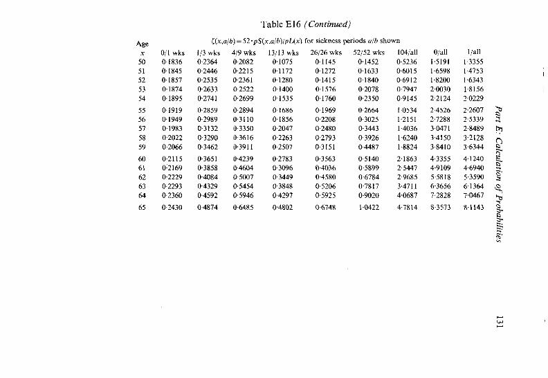
Tablc E16 (Continued)
[(x,a/hl= 52.pS(x,alb)/pL(x) for sickncss periods olb shown
011 wks 113 wks 419 wks 01836 0.2364 0-2082 0.1845 0.2446 0.2215 0.1857 0-2535 02361 0-1874 0.2633 02522 0.1895 0.2741 0.2699
0.1919 0-2859 0.2894 0.1949 0.2989 0.31 10 01983 03132 0-3350 02022 0.3290 0-3616 0.2066 0-3462 0.3911
0.2115 0-3651 0.4239 0-2169 0.3858 04604 0-2229 0.4084 05007 0.2293 0-4329 0.5454 0.2360 04592 0.5946
02430 0.4874 0-6485
13/13 wks 26/26 wks 52/52 wks 0.1075 0-1145 0.1452 0.1172 0.1272 0.1633 0-1280 0.1415 01840 0.1400 0-1576 0.2078 0.1535 0.1760 0.2350
0IbX6 0,1969 0-2664 0.1856 0.2208 0-3025 02047 02480 0.3443 0.2263 02793 0.3926 0-2507 03151 0-4487
0-2783 0.3563 05140 0.3096 0-4036 0.5899 0.3449 0-4580 0.6784 03848 0.5206 0.7817 04297 0.5925 0-9020
0,4802 06748 1.0422

The Analysis of Permanent Health Insurance Data 132
Table E17. Decrement rates and [lye table: conditional on starting at age 30 with initial status healthy. One-week
deferred period basis
Age H to D S to D L to D s m(x) mS(x) mL(n) 30 0.000422 0.000000 0.000422 31 0000427 0060814 0-000986 32 0000438 0.061409 0.001037 33 0.000457 0.061769 0.001088 34 0.000482 0.062190 0.001 147
35 0.000515 0-062661 0001216 36 0-000556 0063170 0.001296 37 0-000605 0-063713 0.001388 38 0.000664 0064285 0001493 39 0000733 0.064878 0.001613
40 0000812 0-065488 0001749 41 0.000902 0.0661 1 1 0~001901 42 0-001004 0.066741 0.002073 43 0-001 1 19 0.067377 0-002265 44 0.001247 0.068017 0-002480
45 0001390 0068657 0.002720 46 0.001548 0.069299 0-002986 47 0.001722 0.069940 0003283 48 0001914 0070582 0003612 49 0.002125 0.071223 0003979
50 0002355 0071867 0004385 51 0.002606 0.072512 0-004837 52 0002880 0.073162 0.005340 53 0.003178 0-073815 0-005899 54 0003501 0-074475 0.006521
55 0.003851 0.075141 0007214 56 0-004231 0075814 0.007987 57 0.004641 0-076495 0008852 58 0-005085 0077182 0009819 59 0.005563 0.077874 0010904
60 0006079 0-078569 0012123 61 0006635 0.079262 0.013494 62 0007233 0-079949 0.015039 63 0.007877 0.080621 0.016782 64 0-008569 0081270 0-018751
65 0.009312 0081881 0-020975
Life table
4x1 4<x) L(.4 1,000,000 0-0009W 999.567
999,091 0.001012 998,589 998,080 0.001062 997,554 997,020 0-001 116 996,468 995,907 0001180 995,325
994,732 0.001254 994,115 993,485 0.001340 992.827 992.154 0001438 991,449 990,727 0.001550 989,969 989,191 0001678 988,372
987.531 0.001822 986,644 985,732 0001984 984,768 983,777 0.002165 982,727 981,647 0002368 980,501 979,322 0.002594 978,071
976,781 0-002847 975,412 974,001 0-003127 972,501 970,955 0-003439 969,311 967,616 0.003785 965,813 963.954 0004170 961,975
959,934 0004597 957.762 955,521 0-005071 953,136 950.676 0-005599 948.056 945,353 0.006185 942,476 939,506 0.006837 936,345
933,082 0007565 929,609 926,024 0.008376 922,207 918.267 0.009283 914,072 909,743 0.010298 905,132 900.374 0011436 895,307
890.078 0.012713 884.509 878,762 0014150 872,642 866,328 0015767 859,605 852,668 0.017590 845,286 837,670 0.019645 829,569
821,214

Part E: Calculation of Probabilities 133
Table E18a. Claim inception rates of type (a) per 10,000 living at giwn deferredperiods at each age: conditional on starting at age 30 with initial
status healthy. One-week deferred period basis.
Age H to S Claim inception rates ia(r,d) per 10,000 living for deferred period dshawn
x 10,00Oa(x) 0 weeks l week 4 weeks l 3 weeks 26 weeks 52 weeks l04 weeks

134 The Analysis o f Permanent Health Insurance Data
Table E18b. Claim inception rates of type (b ) per 10,000 living at given deferred periods at each age: conditional on starting at age 30 with initial
status healthy. One-week deferred period basis
Age H to S Claim inception rates ib(x,d) per I0,OW living far deferred period dshown
x 10,00Oc(x) 0 weeks l week 4 weeks 13 weeks 26 weeks 52 weeks 104 weekr

Part E: Calculation of Prohahiliries 135
Table E19. Sickness rates for each sickness period at each age: conditional on starting at age 30 with initial status healthy One-week deferredperiod basis
--m-
X 011 wks 30 0.2040 31 0.2041 32 0-2024 33 02007 34 0-1989
35 0,1970 36 0.1952 37 01934 38 01417 39 0.1901
40 01885 41 0-1871 42 0.1859 43 0,1848 44 0,1839
45 0.1833 46 0.1829 47 0.1827 48 0.1828 49 0-1832
50 01840 51 0.1851 52 01865 53 0.1884 54 0-1907
55 0-1934 56 0,1965 57 0.2002 58 02043 59 0.2090
60 02142 61 0.2199 62 0-2260 63 02326 64 0.2395
113 wks 01468 0-1558 0.1588 0,1619 0 1650
0.1681 0-1713 0.1745 0.1779 0-1814
0.1851 0,1890 01931 0.1975 0-2023
0.2074 0.2129 02189 02255 0.2326
0.2404 02490 0.2583 0-2686 0.2799
0.2923 0-3060 0.3210 0.3374 0.3555
0.3753 03969 0.4204 0.4458 0-4731
4/9 wks 0.0663 0.0805 00845 0.0887 0.093 1
0-W77 0.1025 0.1076 01129 0,1185
0,1245 0-1308 0.1376 0-1448 0.1 526
0 1609 0.1700 0.1798 0.1904 0-2021
0-2148 0.2287 02440 0.2609 02795
0-3000 0-3228 0.3481 0.3761 04072
04418 04802 0-5226 0-5695 0.6210
13/13 wks 0.0160 0-0263 0.0283 00305 0.0328
0.0353 00380 0-0409 0.0440 00473
00509 0.0549 0.0591 0-0638 0.0689
0.0745 0.0806 00874 0-0949 0.1031
01123 0-1225 0,1339 0.1466 0.1609
0.1769 0.1950 0-2153 0-2383 0.2642
02936 0.3268 0-3644 0.4067 04544
A OF z(x,o/b) in weeks of sickness for sickness periods a/b shown
26/26 wks 52/52 wks 104;all O/all ]/all
OOWO 0.WW 0-4383 0-2343 0.0107 OWOO 0-4969 0.2928 0-0212 00067 0.5234 0.3210 0.0236 0.0192 05482 0.3475 0-0263 0.0315 0.5735 03747
00294 00445 0.6004 0-4034 00327 0.0585 0-6294 U-4342 0.0364 0-0738 0.6609 04675 00406 0-WO7 0.6953 0-5036 0-0452 0,1094 07331 05430
0.0503 0.1301 07748 0.5862 0.0561 01533 0.8209 0.6338 00625 0,1793 0-8722 0.6863 0.0697 0.2086 0-9294 0.7446 00778 0,2417 0.9934 08094
0-0870 0-2791 1.0651 08818 0-0973 03217 1,1458 09629 01089 0.3702 12367 1.0540 0.1221 0,4256 13395 1,1566 01370 04889 1.4558 1-2726
0.1540 05616 1.5878 14039 0.1734 0.6452 1-7381 1.5530 0-1956 0-7416 1.9094 17229 0.2211 04530 21052 1.9168 02503 0.9821 2.3296 2.1389
0.2840 11321 2.5873 23939 0.3228 1.3067 2-8839 2.6874 0.3678 1.5107 32263 3.0261 0.4199 17495 3.6223 3-4180 0.4805 2-03W 4.0816 38726
0-5509 2-3602 4.6153 44011 06329 2.7501 52369 5.0171 0.7286 3.21 19 5.9625 5.7365 08401 37603 6.8108 6-5782 0,9701 4.4133 78040 7.5645

136 The Analysis of Permanent Health Insurance Data
Table E20a. Select table of qlXl+, with 2 years selection. One-week deferredperiod basis
Attained age x
16 17 18 19
20 21 22 23 24
25 26 27 28 29
30 3 1 32 33 34
35
36 ' 37 38 39
40 41 42 43 44
45 46 47 48 49
50 5 1 52 53 54
Select durations ( t ) 2 and over
0~001061 0-001032
0.001006 0000983 0000964 0000950 0.000940
0000935 0.000936 0.000942 0-000954 0-000974
0001000 0.001035 0-001078 0-001130 04Xl1192
0.001266 0.001351 0.001449 0~0015M) 0001687
0-001831 0401992 0002173 0002376 0-002602
0002853 0003134 0,003445 0.003791 0.004175
0004602 0405077 0-005603 0-006190 0.006842

Part E: Calculation of Probabilities
Table E20a. (Continued)
Select table of qlKl+, with 2 years selection. One- week deferred period basis
Attained Select durations ( I ) age x 0 1 2 and over

138 The Analysis of Permanent Health Insurance Data
Table E2Ob. Select table of qIxl+, with 5 years selection. One-week deferredperiod
Attained age X
16 17 18 19
20 21 22 23 24
25 26 27 28 29
30 31 32 33 34
35 36 37 38 39
40 41 42 43 44
45 46 47 48 49
50 51 52 53 54
basis
Select durations (I)
5 and over
0.000983 0.000964 0.000950 0.000940
0.000935 0.000936 0000942 0.000954 0.000974
0.001000 0001035 0.001078 0001 130 0.001 192
0.001266 0.001351 0.001449 0.001560 0001687
0001831 0.001992 0.002 173 0.002376 0.002602
0-002853 0.003134 0.003445 0-003791 0.004175
0.004602 0.005077 0.005603 0406190 0.006842

Part E: Calculation of Probabilities 139
Table EZOb. (Continued) Select table of qlXl+, with 5 years selection. One-week deferredperiod basis
Attained age .Y
55 56 57 58 59
M)
61 62 63 64
Select du
2
0407073 0.007808 0.008628 0.009543 0.010567
0.011716 0.013009 0.014467 0.016118 0-017992
rations ( l )
3
0.007183 0.007935 0.008774 0009712 0.010763
0.01 1943 0-013271 0014770 0.016466 0.018391
5 and over
0.007569 0.008380 0.009287 0.010302 0.01 1439
0.012717 0.014153 0.015770 0.017592 0.019647
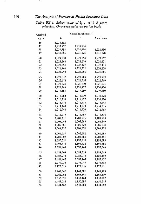
140 The Analysis of Permanent Health Insurance Data
Table E21a. Select table of lIXI+, with 2 years selection. One-week deferredperiod basis
Attained Select durations ( I )
age x 0 1 2 and aver
16 1.235.152

Part E: Calculation of Probabilities
Table E21a (Continued) Select table of with 2 years selection. One-
week deferred period basis
Attained age x
Select durations (l)
1 2 and over
1,135,447 1,136,262 1,126,727 1,127,661 1,117,141 l,118,2Il 1,106,M)Z 1,107,826 1,095,015 1,096,414
1,082,277 1,083,871 1,068,276 1,070,088 1,052,891 1,054,943 1,035,995 1,038,307 1,017,454 1,020.041 I,OOO,WO 1,000,000

142 The Analysis of Permanent Health Insurance Data
Table E21 b. Selecr table of lcl+, with 5 years selection. One-week deferred period basis
Attained Select duralions (I)
age r 0 I 2 3 4 5 and over

Part E: Calculation of Probabilities
Table E21b. (Continued) Select table ~fl~,~,, with 5 yearsselection. One-weekdeferredperiod
basis
Attained Select durations ( l )
age x 0 I 2 3 4 5 and over
55 1,131,440 1,133,659 1,134,708 1,135,406 1,135,903 1,136,262

144 The Analysis of Permanent Health Insurance Data
Table E22a. Select table of iat,,, with 5 years .selection; methods A and B: deferred period (d) 0 weeks. One-week deferredperiod basis
Age x 0
Duration t
3
0.345285
0.346375 0-346672 0346225 0-345089 0-343322
0340983 0338136 0.334842 0.33 11 64 0327164
0322902 0.318437 0-313825 0309119 0304372
0.299629 0-294938 0.290339 0.285873 0281576
0277482 0.273625 0.270033 0266736 0.263761
0.261 133 0.258880 0257026 0255597 0.254619
0254118 0.254123 0-254664 0.255771 0257480
5 and over B
0.346653 0.346204 0345064 0.343293
0340950 0.338097 0.334798 0331114 0.327107
0-322838 0.318365 0-313743 0-309028 0.304269
0.299514 0294809 0.290195 0285712 0.28 1396
0-277281 0273399 0.269780 0-266453 0.263443
0260776 0.258477 0256571 0.255082 0.254033
0.253451 0-253361 0.253789 0254764 0.2563 16
5 and over A
0.346653 0346196 0.345049 0343269
0,3409 l7 0.338055 0-334744 0.331048 0-327028
0322744 0-318254 0.313615 0.308879 0304097
0299317 0.294583 0289937 0.285418 0-281061
0276901 0-272968 0.269290 0-265896 0,2628 10
0.260057 0.257659 0.255639 0254018 0.252816
0-252056 0251758 0-251943 0-252630 0253841

Age r
Part E: Calculation of Probabilities
Table E22a. IContinued) Select table of iatl+, with 5 years selection: methods A and B. deferrtdperiod ( d ) 0 weeks. One-week deferred period basis
Duration i
2 3 5 and over B
0.258473 0.261269 0.264736 0-268904 0.273806
0.279466 0.285905 0293128 0.301126 0.309858
5 and over A
0.255594 0257906 0.260793 0.264262 0268316
0272945 0-218123 0-283800 0.289890 0296263

146 The Analysis of Permanent Health Insurance Data
Table E22b. Select table of iafXl+, with 5 years selection: methods A and B: deferredperiod (d) I week. One-week deferred period basis
Duration r Age x 0 5 and over
B
0.11 1288 0113169 0.114849 0116336
0.117639 0.118769 0.119739 0.120563 0.121255
0121832 0,122309 0.122703 0.123031 0.123312
0.123563 0.123801 0124045 0.124313 0,124623
0.124992 0125440 0,125985 0 126645 0.127442
0-128393 0.129521 0.130846 0.132392 0.134183
0.136245 0.138606 0.141294 0.144342 0.147784
S and over A
0111288 0.113166 0.1 14844 0.116328
0-1 17627 0.1 18754 0.1 19720 0120539 0121226
0.121796 0.122266 0.122652 0-122972 0.123242
0,123481 0123706 0.123935 0,124185 0.124474
0124821 0.125242 0-125756 0.126381 0.127136
0.128039 0-129110 0130370 0-131840 0.133540
0.135495 0.137728 0.140265 0.143132 0.146357

Age x
Part E: Calculation of Probabilities 147
Table E22b. (Continued) Select table of iafxl+, with 5 years selection: methods A and B:
deferred period (d) I week. One-week deferred period basis
Duration t
2 3 5 and over B
0151658 0.156002 0,160858 0,166270 0.1 72283
0.178942 0.186288 0194359 0.203179 0-212756
5 and over A
0.149968 0-1 53993 0.158461 0.163399 0.168828
0174765 0.181217 0188173 0,195597 0.203420

148 The Analysis of Permanent Health Insurance Data
Table E22c. Select table of ia&+, with 5 years selection: merhods A and B: deferredperiod (d) 4 weeks. One-week deferred period basis
Duration r Age x
16 17 18 19
20 21 22 23 24
25 26 27 28 29
30 3 1 32 33 34
35 36 37 38 39
40 41 42 43 44
45 46 47 48 49
50 51 52 53 54
5 and over B
0.014031 0014796 0015569 0.016352
0.017145 0017946 0.018758 0-019581 0.020416
0.021266 0.022131 0.02301 5 0.023921 0-024852
0025812 0026806 0.027838 0-028915 0.030042
0.031228 0-032479 0.033806 0035217 0.036724
0.038340 0040079 0.041955 0.043988 0.046196
0.048602 0.051231 0-054112 0.057276 0-060759
i and over A
0.014031 0014795 0015569 0.016351
0.017143 0.017944 0.018755 0-019577 0-02041 1
0.021260 0022124 0-023006 0-023910 0.024838
0-025795 0.026785 0-027813 0028885 0.030007
0.031185 0032428 0033744 0.035143 0.036636
0.038234 0039951 0.041 802 0-043804 0.045974
0-048334 0450907 0-053717 0.056795 0.060171

Age x
55 56 57 58 59
60 61 62 63 64
Part E: Calculation of Probabilities 149
Table E22c. (Continued) Select table of iatl+, with 5 years selection: methods A and B: deferredperiod (d) 4 weeks. One-week deferredperiod basis
Duration I
5 and aver B
0.064602 0-068850 0-073554 0.078772 0084565
0091003 0098159 01061W 0.114933 0- 124704
5 and over A
0.063881 0067962 0072457 0.077410 0.082868
0088878 0.095485 0102730 0.110642 0 1 19230

150 The Analysis of Permanent Health Insurance Data
Table E22d. Select table of ia&+, with 5 years selection: methods A and B: deferredperiod (d) 13 weeks. One-week deferred period basis
Age X
16 17 18 19
20 21 22 23 24
25 26 27 28 29
30 31 32 33 34
35 36 37 38 39
40 41 42 43 44
45 46 47 48 49
50 51 52 53 54
Duration r
3 4 5 and over B
0.001755 0~001901 0002054 0.002214
0.002384 0002562 0.002749 0.002945 0.003152
0003370 0003600 0.003843 0~004099 0.00437 1
0.004659 0.004965 0005291 0.005639 0.006012
0006412 0.006842 0007306 0.007809 0008354
0.008947 0.009594 0.010303 0.01 1080 0.011935
0012880 0,013925 0.015085 0016377 0.017817
5 and over A
0.001755 0401901 0-002053 0.002214
0.002383 0-002561 0.002748 0.002945 0.003152
0403369 0.003599 0.003841 0.004097 0.004368
0-004655 0.004961 0005286 0.005633 0.006004
0.006403 0.00683 1 0007293 0.007792 0-008334
0.008922 0.009564 0410265 0.01 1033 0.011878
0.012808 0,013836 0414975 0016238 0.01 7644

Part E: Calculation of Probabilities
Table E22d. (Continued) Select table of ia&+, with 5 years selection: methods A and B: deferredperiod (d) 13 weeks. One-week deferredperiod basis
Duration I 0 I 2 3 4 5 and over 5 and ova
B A
0.015050 0.0197W 0.019603 0019532 0.019475 0.019429 0-019212 0-016505 0.021 577 0.021456 0.021366 0.021295 0021237 0-020962 0-018152 0-023698 0023546 0.023432 0.023342 0.023269 0-022920 0.020024 0426103 0.025911 0025766 0.025651 0.025557 0.025114 0-022160 0.028837 0.028592 0.028407 0028260 0028139 0.027573
0.024605 0.031955 0031641 0-031403 0431213 0.031058 0.030331 0027412 0.035521 0.035117 0.034808 0434562 0-034361 0033423 0.030648 0.039610 0-039086 0.038683 0.038362 0.038101 0036886 0.034390 0.044312 0.043627 0-043100 0.042679 0.042337 0.040754 0.038732 0.049732 0-W831 0-048135 0047579 0.047129 0.045058

152 The Analysis of Permanent Health Insurance Data
Table E22e. Select table o f i a t l + , with 5 years srlectiun: methods A and B: deffrredperiod (d) 26 weeks. One-week deJerredperiod basis
Duration 1
Agc x 0 1 2 3 4 5 and over 5 and over B A
16 0.000141 17 0.0001 58 0.000307 18 0.000176 0000343 0-000343 19 0.000196 0.000383 0-000383 0-000382

Age X
Part E: Calculation of Probabilities
Table E22e. (Continued) Select table of iafxl+, with 5 years selection: methods A and E: deferred period (d) 26 weeks. One-week deferred period basis
Duration t
0 I 2 3 4 5 and over 5 and over B A
0-W5465 0.010567 0.010512 0.010473 0.010442 0.010417 0.010300 O.oO6IlZ 0.01 1802 001 1732 0011682 0011643 0011611 0.011460 0006856 0-013218 0013129 0.013064 0.013014 0.012972 0.012777 0.007714 0.014846 0.014732 0.014649 0.014583 0.014529 0.014276 0.008707 0.016725 0016578 0016469 0016383 0016313 0015983
0.009860 0.018901 0.018709 0.018566 0-018453 001 8361 0.01 7929 0-011205 0021426 0021175 0.020987 0-020837 0.020716 0.020149 0-012778 0024369 0.024038 0.023788 0.023589 0.023428 0.022679 0.014625 0.027808 0.027368 0.027034 0-026769 0026554 0025559 0016803 0031839 0031251 0.030802 0.030445 0.030157 0.028829

154 The Analysis of Permanent Health Insurance Data
Table E22f. Select table of iafXl+, with 5 years selection: methods A and B: deferredperiod (d) 52 weeks. One-week deferredperiod basis
Age x
16 17 18 19
20 21 22 23 24
25 26 27 28 29
30 3 1 32 33 34
35 36 37 38 39
40 41 42 43 44
45 46 47 48 49
50 51 52 53 54
Duration t
3 4 5 and aver B
0.000172 0.000194 0.000218 0.000244
0000274 0~000306 0.000341 0-000380 0.000423
0.000470 0.000522 0.000578 0-000641 0.000710
0.000786 0.000869 0-000962 0-001064 0.001177
0-001303 0.001442 0-001597 0.001770 0001964
0-002181 0002424 0.002698 0.003007 0-003357
0.003753 0404204 0004718 0.005305 0005978
5 and over A
0000172 0.000194 0000218 0.000244
0.000273 0000306 0.000341 0.000380 0.000423
0000470 0400521 0.000578 0.000641 0400709
0.000785 0000869 0.000961 0-001063 0.001 176
0-001301 0.001440 0-001594 0.001767 0-001959
0.002175 0.002416 0402688 0-002994 0-W3340
0.003732 0-004177 0-004682 0.005259 0-005918

Age x
Part E: Calculation of Probabilities
Table E22f. (Continuedj Select table of iat',,,, with 5 years selection: methods A and B: deferred period ( d ) 52 weeks. One-week deferred period basis
Duration 1
2 3 5 and over B
0.006751 0-007642 0.008671 0.009863 0.01 1247
0-012859 0.014738 0-016935 0.019506 0.022519
5 and over A
0.006674 0-007541 0-008539 0.009690 0.011018
0-012554 0.014332 0016390 0.018772 0421 524

1 S6 The Analysis of Permanent Health Insurance Data
Table E22g. Select table o f iatxl+, with S years selection: methods A and B: deferred period ( d ) 104 weeks. One-week deferred period basis
Age x
16 1 l 18 19
20 21 22 23 24
25 26 27 28 29
30 31 32 33 34
35 36 37 38 39
40 41 42 43 44
45 46 41 48 49
50 51 52 53 54
Duration I 3
0000056
0-000064 0-000074 0-000084 0.000096 0-000110
0-000125 0.000142 0-000161 0-000182 0.000205
0.000232 0.000261 0-000294 0400331 0-000371
0.000417 0-000468 0.000525 0-000589 0.000660
0.000741 0.000831 0-000933 0401047 0-001 177
0.001324 0-001490 0401680 0.001895 0-002142
0.002425 0402749 0-003123 0.003555 0-004055
5 and over B
0400074 0-000084 0-000096 0-0001 10
0-000125 0-000142 0-000161 0.000182 0-000205
0.000232 0-000261 0.000294 0000330 0.000371
0.000417 0.000468 0-000525 0400588 0-0006M)
0400740 0-000830 0.000932 0.001046 0-001 175
0401321 0-001481 0-001676 0.001891 0-002136
0.002417 0002739 0.003110 0.003538 0004033
5 and over A
0.000074 0000084 0000096 0000110
0.000125 0.000142 0-000161 0.000182 0-000205
0.000232 0-000261 0.000294 0-000330 0.000371
0-000416 0.000467 0-000524 0.000588 0-000659
0-000139 0-000829 0.000930 0-001044 0-001112
0.001317 0-001482 0-001669 0401882 0-002125
0.002403 0-002721 0403086 0-003507 0-003992

Par! E: Calculation of Probabililies
Table E22g. (Continued) Select table of ia$,+, with 5 years selec!ion: methods A and B: deferredperiod (d) 104 weeks. One-week deferredperiod basis
Age l 0 Duration I
2 3 5 and over B
0.004rn8 0.005276 0.006056 0.006969 0.008040
0.009301 0-010789 0.012550 0014640 0.017126
5 and over A
0.004554 0005205 0.005962 0006843 0.007873
0009076 0.010487 0.012141 0.014083 0-016362

158 The Analysis of Permanent Health Insurance Data
Table E23a. Select table of z#+, with 5 years selection: methods A and B: sickness period (a/b) O/I weeks. One-week deferred period basis
Duration t
Age r
16 17 18 19
20 21 22 23 24
25 26 27 28 29
30 31 32 33 34
35 36 37 38 39
40 41 42 43 44
45 46 47 48 49
50 51 52 53 54
5 and over B
0.2080 02091 0.2098 0.2100
02100 0.2096 0.2089 0.2079 0.2068
0.2054 0.2039 02023 0.2006 0.1988
0.1970 01953 0.1935 0.1918 0.1902
01887 0,1874 0 1862 0.1851 0,1843
0.1837 0-1834 0.1833 0.1835 0-1841
0.1850 0-1862 0.1879 0- 1899 0.1925
5 and over A
0.2080 0-2091 0.2097 0-2100
0.2099 0.2095 0.2088 0-2079 0.2067
0.2054 0.2038 0-2022 0.2005 01987
0.1969 0.1951 0.1933 01916 0.1900
0.1885 0.1871 01858 0.1847 01839
0,1832 0,1828 0,1826 01828 0,1832
01839 0.1850 0,1865 01884 0.1906

Age x
Parr E: Calculation of Probabilities
Table E23a. (Continued) Select table ofzf$+, n,ith 5 Tears selecrion: method.$ A and B:
sickness period (a/b) OII weeks. One-week deferred period basis
Duration t
3
0.1965 0-2003 0-2046 0.2096 0-2153
0.2217 0-2289 0.2370 02459 0.2558
5 and over B
0.1955 0.1991 02032 0.2079 0.2132
02193 0.2260 02334 0.2416 0.2505
5 and over A
0,1933 0,1965 0.2002 02043 0.2090
02141 0.2198 0.2260 0.2326 0-2395

160 The Analysis of Permanent Health Insurance Data
Table E23b. Select table of zKP+, with 5 years selection: methods A and B: sickness period (a/b) 113 weeks. One-week deferred period basis
Age x
16 17 18 19
20 21 22 23 24
25 26 27 28 29
30 31 32 33 34
35 36 37 38 39
40 41 42 43 44
45 46 47 48 49
50 5 1 52 53 54
Duration I I 2 3 4 5 and over
B
0.1208 0,1248 0,1286 01323
0.1359 0.1394 01428 0.1461 0.1494
0.1525 0.1557 0-1588 0-1619 01650
01681 0.1713 0-1746 0.1780 0.1815
0-1853 0.1892 0-1934 0.1979 02027
02079 0.2135 02197 0.2264 0.2337
02417 0.2505 02602 02708 0.2826
5 and over A
0,1208 0,1248 0,1286 01323
0,1359 01394 0,1428 0,1461 01493
0,1525 01556 0,1587 01618 0,1649
0,1680 0.1712 0- 1744 0.1778 0.1813
0-1850 0,1889 0-1930 01975 0-2022
0-2073 0.2129 0-2189 0.2254 0.2326
02404 0.2489 02583 0.2686 0.2799
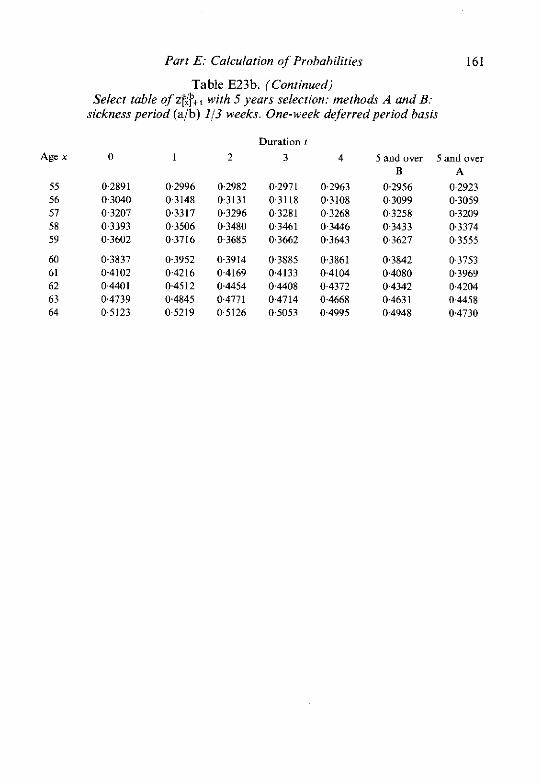
Age x
Part E: Calculation of Probabilities
Table E23b. (Continued) Select table of z@+, with 5 years selection: method? A and&
sickness period (a/b) 1/3 weeks. One-week deferred period basis
Duration I 0 1 2 3 4 5 and over S and over
B A 0-2891 0.2996 0.2982 0.2971 0.2963 0-2956 0.2923 0.3040 03148 0-3131 03118 0,3108 03099 0-3059 0.3207 0.3317 0.3296 03281 03268 0.3258 0.3209 03393 0.3506 0.3480 0.3461 0.3446 0-3433 0.3374 0-3602 03716 03685 0.3662 0.3643 0-3627 03555
0.3837 0.3952 0-3914 03885 0.3861 0.3842 03753 0-4102 0.4216 0.4169 0,4133 0-4104 0.4080 0.3969 0.4401 0-4512 0-4454 0.4408 0-4372 04342 0.4204 0.4739 0.4845 0.4771 04714 0-4668 0.4631 04458 05123 05219 0.5126 0.5053 0-4995 04948 0.4730

162 The Analysis of Permanent Health Insurance Data
Table E23c. Select table of zr$+, with 5 years selection: methods A and B. sickness period (ajb) 419 weeks. One-week deferred period basis
Age x
16 17 18 19
20 2 I 22 23 24
25 26 27 28 29
30 3 1 32 33 34
35 36 37 38 39
40 41 42 43 44
45 46 47 48 49
50 51 52 53 54
Duration 1
I 2 3 4 5 and over B
00461 0.0491 0.0522 0.0554
0-0586 0.0620 0-0655 0-0690 0.0727
0-0765 0.0804 0.0845 00887 0.0931
0.0977 0,1026 0,1076 0.1130 0,1186
0.1246 0.1310 0-1378 0.1450 01529
0-1613 0.1705 0-1804 0.1912 0.2030
0.2159 0.2301 02458 0.2630 0.2821
i and over A
04461 0.0491 00522 0.0554
0.0586 00620 0.0655 0.0690 00727
0.0765 0.0804 0-0845 0.0887 0-W31
0.0977 0.1025 0-1075 01128 0.1185
0,1244 01307 0,1375 0.1447 0.1 525
0.1609 0-1699 0.1797 0-1904 0.2020
0-2147 0.2287 0.2440 02608 0.2794

Age x
Part E: Calculation of Probabilities 163
Table E23c. (Continued) Select table of z@+, with 5 years selection: methods A and B:
sickness period (a/b) 419 weeks. One-week deferredperiod basis
Duration t
3
0.3050 0.3290 0.3558 03858 04195
0.4573 0-4999 0.5480 0.6022 0.6633
5 and over B
0-3034 0.3270 0-3533 03827 0.4155
04523 0.4935 0.5398 05915 06495
5 and over A
0.3000 0.3227 0-3480 03760 0.4072
0,441 7 0.4801 0.5226 05694 0.6210

164 The Analysis of Permanent Health Insurance Data
Table E23d. Select table of r$p+, with 5 years selection: methods A and B. sickness period (aib) 13/13 weeks. One-week deferred period basis
Duration r Age s
16 17 18 19
20 21 22 23 24
25 26 27 28 29
30 3 1 32 33 34
35 36 37 38 39
40 41 42 43 44
45 46 47 48 49
50 51 52 53 54
5 and over B
0.01 16 0.0127 00139 00151
00164 0.0178 0-0193 0-0209 0.0225
0-0243 0.0262 00283 0.0305 0-0328
0.0353 0-0380 0.0409 0.0440 00473
0.0510 00549 0.0592 00639 0,069 1
00747 0.0809 0.0877 0-0952 0-1036
01129 0.1233 0-1348 0.1478 0.1624
I and over A
0.0116 00127 00139 0.0151
0.0164 001 78 00193 0.0209 00225
0.0243 0-0262 0.0283 0.0304 0-0328
0.0353 00379 0.0408 0-0439 0-0473
00509 0.0548 00591 00638 0.0689
00745 00806 0.0874 00948 0.1031
0.1123 0.1225 0-1339 0.1466 01609

Age x
Parr E: Calculation of Probabilities
Table E23d. (Continued) Select table of z?$+~ with 5 years selecrion: methods A and B:
sickness period (a/b) 13/13 weeks. One-week deferredperiod basis
Duration f
0 I 7 3 4 5 and over 5 and over B A
01186 01814 01805 0.1798 0,1793 0-1789 0.1769 01313 0.2007 0.1995 0-1987 01980 0-1975 0-1949 01458 02226 0.2212 0.2201 02192 0.2185 02153 0-1623 02477 0.2458 0.2444 0.2433 0.2424 02382 0.1813 02764 0-2740 0.2722 0.2708 0.2696 0.2642
0-2033 0.3093 0.3063 0.3039 03021 0.3006 02935 0.2286 0.3474 0.3434 0.3403 03379 0.3359 03268 0.2581 0.3913 0-3861 03821 0.3789 03763 0.3643 0.2924 0-4423 0.4354 0.4301 0-4259 0.4225 04067 0.3325 0.5016 0-4924 0.4854 0.4798 04752 0.4543

166 The Analysis of Permanent Health Insurance Data
Table E23e. Select table of z#+, with 5 years selection: methods A and B: sickness period (aib) 26/26 weeks. One-week deferred period basis
Age x
16 17 18 19
20 21 22 23 24
25 26 27 28 29
30 31 32 33 34
35 36 37 38 39
40 41 42 43 44
45 46 47 48 49
50 5 1 52 53 54
Duration t I 2 3 4 5 and over 5 and over

Age x
55 56 57 58 59
60 61 62 63 64
Part E: Calculation of Probabilities
Table E23e. (Continued) Select table of z@+, with 5 years selection: methods A and B:
sickness period (a/b) 26/26 weeks. One-week deferred period basis
Duration t 2 3 5 and over
B 02109 0.2371 0-2673 0.3020 0.3421
0.3884 04422 0.5046 0.5772 06616
5 and over A
0-2085 0.2340 0.2632 02967 0.3351
0.3793 0.4300 0.4884 0.5555 06325

168 The Analysis of Permanent Health Insurance Data
Table E23f. Select table of z$p+, with 5 years selection: methods A and B: sickness period (a/b) 52/52 weeks. One-week deferred period basis
Age x
16 17 18 19
20 21 22 23 24
25 26 27 28 29
30 31 32 33 34
35 36 37 38 39
40 41 42 43 44
45 46 47 48 49
50 51 52 53 54
Duration I
5 and ovet B
0.0058 0.0066 00074 0.0084
00095 0.0107 00120 0.0135 0.0151
00169 0.0189 0.0212 0-0236 0.0263
0-0294 0.0327 0-0364 0.0406 0-0452
0-0504 0.0562 0.0626 0-0699 0.0780
0-0872 0-0975 0-1093 0.1226 0.1377
0.1549 0-1746 0.1971 0-2230 0-2528
5 and over A
0.0058 0.0066 0.0074 0.0084
0-0095 0.0107 OOl20 0.0135 0~0151
00169 00189 0.021 1 00236 0.0263
00293 0.0327 0.0364 0.0405 00452
0.0503 0.0561 0.0625 0.0697 0.0778
0-0869 0.0972 0-1088 0.1220 0- 1370
0.1540 0-1734 0,1956 0-2210 02503

Age x
Part E: Calculation of Probabilities
Table E23f. (Continued) Select table of zf$+, with 5 years selection: methods A and B:
sickness period (a/b) 52/52 weeks. One-week deferredperiod basis
Duration r 0 I 2 3 4 5 and over 5 and over
B A
00000 0.1584 0.2902 0.2889 02880 02872 0-2839 0.0000 0.1805 0.3310 03293 03281 0-3271 0-3228 00000 0-2063 0.3785 0.3763 0.3747 0.3735 0.3677 0.0000 0.2364 0.4340 04312 04291 04274 0-4199 00000 0-2718 0.4992 0.4954 0.4926 0.4905 0.4804
00000 0.3135 0.5758 0.5708 0.5672 0-5643 0.5508 0.00W 0.3628 0.6664 0.6597 0-6548 0-6509 0.6328 0.0000 0.4213 07737 07648 0-7581 0-7528 0-7285 00000 0-4911 0.9012 0.8892 0.8802 04730 0.8400 0,0000 0.5744 1.0535 1.0372 1.0248 1-0150 0.9700

170 The Analysis of Permanent Health Insurance Dam
Table E24a. Sickness rates z(x,l04/all,x-xo). One-week deferredperiod basis
Attained Entry age xo

Part E: Calculation of Probabilities 171
Table E24a. (Continued) Sickness rates z(x.l04/aN,x -xo). One-week deferred period basis
Attained Entry age xo agex 16 17 18 19 20 21 22 23 24 25
55 1,1416 1.1415 1,1414 1.1412 1.1410 1.1408 1.1404 1.1400 1,1395 1,1388 56 1.3158 1.3157 1.3156 1.3154 1.3152 1.3150 1.3147 1.3143 1.3138 1.3132 57 1.5193 1.5192 1.5191 1.5190 1.5188 15186 1-5183 1-5179 1.5174 1.5168 58 1.7578 1.7577 1.7576 1.7574 1.7573 1.7570 1.7568 1.7564 1.7559 1.7554 59 2.0378 2.0378 2.0377 2.0375 2.0374 2.0371 2-0369 2-0365 2.0361 2.0355

172 The Analysis of Permanent Health Insurance Data
Table E24b. Sickness rates z(x,l04/all,x - x o ) . One-week deferredperiod basis
Attained Entry age xo

Part E: Calculation of Probabilities
Table E24c. Sickness rates z ( x , l 0 4 / a N , x x ~ ) . One-week deferredperiod basis
Attained Entry age xo age x
36 37 38 39
40 41 42 43 44
45 46 47 48 49
50 51 52 53 54
55 56 57 58 59
60 61 62 63 64

174 The Analysis of Permanent Health Insurance Data
Table E24d. Sickness rates z(x,l04/aN,x-xo). One-week deferred period basis
Attained Entry age xo age x
46 47 48 49
50 51 52 53 54
55 56 57 58 59
60 61 62 63 64

Part E: Calculation o f Probabilities
Table E24e. Sickness rates z(x,l04/aN.x -xo). One-week deferredperiod basis
Attained age x 56
56 OWJOO 57 0.0000 58 0.1731 59 03327
60 0.9292 61 1-3791 62 14967 63 2.4975 64 3-1999
Entry age xo
58 59 M) 61 62 63 64

176 The Analysis of Permanent Health Insurance Data
Table E25. Averageprobabilities, pi(x,d), of survitlal while sick from duration 0 ro duration d , sickness commencin~ between ages X andx+ l , using values conditional
on entry at age 16. One-week deferredperiod basis
Duration d (weeks)

Part E: Calculation of Probabilities 177
Table EX. iContinued) Acerageprobahilitiur, pi(x,d), ofsuraiual while sick from duration 0 to duration d.
sickness commencing between ages X and X+ l , using values conditional on entry ar age 16. One-week deferredperiod basis
Duration
13 0-076658 0-082919 0.089689 0-097007 0.104918
0 11 3469 0.122713 0.132705 0.143505 0.155177
d (weeks)
26 OM2330 0.046704 0-051526 0-056843 0.062704
0.069165 0076285 0.084134 0-092782 0-102313

178 The Analysis of Permanent Health Insurance Data
Table E26. Select table of qlXl+, with 5 wars selection. Four-week deferredperiod
Attained Age x
16 17 18 19
20 21 22 23 24
25 26 27 28 29
30 31 32 33 34
35 36 37 38 39
40 41 42 43 44
45 46 47 48 49
50 51 52 53 54
basis
Select duratians ( t )
5 and over
0.000821 0-000804 0400791 0-W0782
0.000778 0-000779 0.000785 0-000797 0.0008 14
0.000838 0.000868 0.000906 0000952 0.001007
0001072 0.001 146 0.001232 0001330 0.001441
0.001 567 0.001 708 0-001866 0.002043 0.W2241
0002461 0-002706 0-002978 0.003281 0.003617
0.003991 0-004407 0.004870 0005387 0005964

Parr E: Calcularion of Probabilities 179
Table E26. (Continued) Select table of qr,l+r with 5 years selection. Four-week deferred period basis
Attained Age X
55 56 57 58 59
60 61 62 63 64
Select dul
2
0.006246 0.006915 0-007667 0.008515 0.009478
0.010574 0.011831 0.013280 0-014963 0-016929
5 and over
0.00661 1 0.007338 0.008157 0.009084 0.010137
0-011338 0.012715 0.014300 0016134 0.018266

180 The Analysis of Permanent Health Insurance Data
Table E27. Select table of ia&+, with 5 years selection: merho& A and B: deferredperiod ( d ) 4 weeks. Four-week deferredperiod basis
Duration t 2 3 5 and over
B
0.008336 0.009095 0.009867 0-010647
0.011431 0.012216 0012999 0.013776 0014545
0.015306 0.016058 0.016802 0-017537 0418268
0-018996 0.019725 0.020460 0.021207 0.021971
0022760 0.023583 0.024448 0.025367 0-026352
0-027416 0.028575 0.029846 0.031250 0.032810
0.034553 0.036510 0.038720 0.041224 0.044076
5 and over A
0-008336 0~009095 0.009866 0.010647
0.011431 0.012216 0.012998 0013774 0.014543
0-015304 0416055 0016797 0.017532 0-018261
0.018987 0.019715 0.020448 0.021 191 0.021952
0.022738 0-023556 0.024416 0025329 0.026306
0-027361 0.028509 0.029767 0031 155 0.032696
0.034415 0.036344 0-038517 0.040977 0-043771

Part E: Calculation of Probabilities
Table E27. (Continued) Select table of iafxl+, with 5 years selection: methods A and B: deferred period ( d ) 4 weeks. Four-week deferred period basis
Duration I 0 1 2 3 4 5 and over 5 and over
B A
0.044500 0-047795 0.047632 0-047510 0.047413 0.047334 0-046958 0.048134 0.051649 0.051446 0-051293 0.051172 0.051074 0.050606 0-052345 0.056106 0-055850 0.055657 0.055505 0.055381 0.054794 0.057247 0.061281 0060955 0.060710 0060516 0.060358 0.059617 0.062983 0-067318 0.066899 0066583 0.066332 0.066130 0.065186
0-069725 0.074390 0073845 0.073432 0.073107 0.072844 0.071632 0.077691 0.082710 0.081992 0.081449 0481020 0.080676 0-079105 0.087151 0.092541 0.091583 0-090857 0490287 0.089830 0.087776 0-098444 0.104202 0102908 0.101927 0-101159 0.100546 0.097832 0.111996 0.118089 0.116315 0.114973 0.113924 0-113091 0.109471

182 The Analysis of Permanent Health Insurance Data
Table E28a. Select tahle of z@+, with 5 yearr selection: meth0d.i A and B: sickness period (ajb) 419 n,eeks. Four-~veek deferred period hasis
Age x
16 17 18 19
20 21 22 23 24
25 26 27 28 29
30 31 32 33 34
35 36 37 38 39
40 41 42 43 44
45 46 47 48 49
50 5 I 52 53 54
Duration I
I 2 3 4 j and over 5 and over

Age x
Part E: Calculation of Probabilities
Table E28a. (Continued) Select table of z@+, with 5 years selection: methods A and B:
sickness period (a/b) 419 weeks. Four-week deferred period basis
Duration 1
2 3 5 and over B
0.222I 0.2423 0.2657 02928 0.3244
0.3614 0.4048 0.4559 0.5161 0.5873
5 and over A
0.2203 0.2401 0.2628 0.2892 0.3198
0-3553 0.3969 0-4454 0.5022 0.5685

184 The Analysis of Permanent Health Insurance Data
Table E28b. Sdert ruhle of zf$+, with 5 years selection: methods A and B. sickness ~ e r i o d (a/b) 13/13 weeks. Four-week deferred period basis
Duration t
Age x
16 17 18 19
20 21 22 23 24
25 26 27 28 29
30 31 32 33 34
35 36 37 38 39
40 41 42 43 44
45 46 47 48 49
50 5 1 51 53 54
5 and over B
0-0068 04477 0-0087 0-0098
00109 0.0121 0.0133 00146 00160
04175 00190 0.0206 00223 0.0241
00260 0-0279 0.0300 0.0323 0-0346
0.0372 00399 00429 0.0461 0-0496
0-0534 0.0577 0-0624 0.0677 0-0736
0.0802 00877 0G963 0-1062 0-1175
j and over A
0.0068 0.0077 00087 0.0098
0.0109 0.0121 00133 00146 0.0160
0-0175 0.0190 0-0206 0.0223 0-0241
0-0260 00279 00300 0-0322 0.0346
0-0372 0-0399 00428 00460 0.0495
00533 0.0576 00622 00675 0.0733
0-0799 04873 00958 0,1055 0,1167

Age x
55 56 57 58 59
60 61 62 63 64
Part E: Calculation of Probabilities
Table E28b Continued) Select table o f z@+, with 5 years selection: melhodr A and B:
sickness period (alb) 13/13 weeks. Four-week deferred period basis
Duration t
2 3 5 and over B
0,1306 01459 0.1637 0-1847 0.2094
0-2388 02737 03156 0.3657 0-4260
5 and aver A
0.1296 0.1445 0.1620 0.1824 02064
0.2348 0.2684 0-3083 0.3558 0.4124

186 The Analysis o f Permanent Health Insurance Data
Table E28c. Select table of zf$+, with 5 years selection: method.^ A and B: sicknesperiod (a/b) 26/26 weeks. Four-week deferredperiod basis
Age x
16 17 18 19
20 21 22 23 24
25 26 27 28 29
30 31 32 33 34
35 36 37 38 39
40 41 42 43 44
45 46 47 48 49
50 51 52 53 54
Duration r
2 3 5 and over B
00041 0.0047 0.0054 00062
0.0071 0.0080 0.0091 0-0102 0.01 14
0-0127 0.0141 0.0156 0-0172 0.0190
0-0209 0.0230 0.0252 00276 0.0302
0.033 1 0.0362 0-0397 0.0435 0.0477
0-0524 0.0576 00635 0.0701 00776
0.0862 0.0960 0,1073 0 l204 0,1356
5 and over A
00041 0.0047 0.0054 00062
0.0071 00080 0.0091 00102 0.0114
0.0127 0.0141 0.0156 0.0172 0.0190
0.0209 0-0230 0.0252 0.0276 0-0302
0.033 1 00362 0-0396 0.0434 00476
0.0523 0-0575 0.0633 0-0699 0.0773
0.0858 0.0955 0,1067 0.1196 0.1346

Part E: Calculation of Probabilities
Table E28c. /Continued) Select table of @+, with 5 years selection: methods A and B:
sickness period (a/b) 26/26 weeks. Four-week deferred period basis
Age x 0
Duration r
3 4 5 and over B
0.1534 0-1743 0,1990 0-2284 0.2635
0.3056 03565 0.4181 0.4930 0.5846
5 and over A
0-1521 0.1727 0- 1969 0.2256 02597
0.3W5 0.3495 0.4084 04797 0.5658

188 The Analysis o f Permanent Health Insurance Data
Table E28d. Select table of z#F+, with 5 years selection: methods A and B: sicknessperiod (a/b) 52152 weeks. Four-week deferredperiod basis
Age X
16 17 18 19
20 21 22 23 24
25 26 27 28 29
30 31 32 33 34
35 36 37 38 39
40 41 42 43 44
45 46 47 48 49
50 51 52 53 54
Duration I
I 2 3 4 5 and over B
00033 00039 0.0045 0.0053
0-0061 0.0071 0.008 1 0.0093 0-0106
0.0120 0-0136 0.0153 0.0172 0.0193
0.0216 00241 0.0268 00298 0.0332
0.0369 0.0410 0.0455 0.0506 0.0562
0.0626 0-0698 0.0779 0.0872 0-0977
0.1099 0.1239 0-1401 0-1590 0.1812
5 and over A
0.0033 0.0039 0,0045 00053
0.0061 0.0071 00081 0.0093 0.0106
0-0120 0.0136 0.0153 0-0172 00193
00215 0.0240 0.0268 0.0298 0-0331
0.0368 0.0409 0.0454 0.0505 0.0561
00625 0.0696 0.0777 0-0869 0.0974
0.1094 0-1233 0.1393 0-1580 0-1799
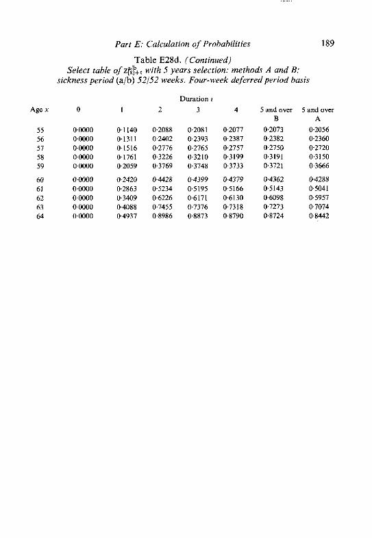
Age x
55 56 57 58 59
60 61 62 63 64
Part E: Calculation of Probabilities
Table E28d. (Continued) Select table of zr&+b,, with 5 years selection: methods A and B:
sickness period (a/b) 52/52 weeks. Four-w,eek deferredperiod basis
Duration I
2 3 5 and over 5 and aver B A
0.2073 0-2056 02382 0.2360 0.2750 0.2720 0.3191 0.3150 0.3721 03666
0.4362 0.4288 0.5143 0.5041 0.6098 0.5951 0.7273 0.7074 04724 0.8442

190 The Ana/.vsis of Permanent Health Insurance Data
Table E29a. Sickness rates z(x,I04/all,x - xo). Four-week deferred period basis
Attained Entry age r a agex 16 17 18 l 9 20 21 22 23 24 25

Part E: Calculation of Probabilitie.~
Table E29a. (Continued) Sickness rates z(x,l04/all,x-xo). Four-week deferredperiod basis
Attained Entry age xa age x 16 17 18 19 20 21 22 23 24 25
55 0.8141 0.8140 04140 0-8139 04138 04136 0.8134 0.8132 0.8128 0.8124 56 0.9399 0.9398 0-9398 0.9397 0.9396 0-9395 0-9393 0.9390 0.9387 0.9383 57 10885 1.0884 1.0884 1.0883 1-0882 1.0881 1.0879 1.0877 1-0874 1.0870 58 1.2649 1.2648 1-2648 12647 1.2646 1.2645 1.2643 12641 1.2638 1.2634 59 14753 1-4753 1-4753 1.4752 1.4751 1-4750 1.4748 1.4746 1.4743 1.4740
M) 1.7278 1.7278 1.7277 1-7277 1.7276 1.7275 1.7273 17271 1-7268 1.7265 61 20323 2.0323 2.0322 2.0322 2.0321 2-0320 2.0318 2.0316 2.0314 2.0311 62 2,4017 2.4017 2-4016 24016 2.4015 2.4014 2.4012 24010 2.4008 2.4005 63 28524 2.8524 2.8523 2.8523 2-8522 2-8521 2.8519 2.8518 2-8515 28512 64 3.4055 3.4055 3.4054 3-4054 3.4053 3.4052 3.4051 3.4049 3.4047 3.4044

192 The Analysis of Permanenr Health Insurance Data
Table E29b. Sickness rates z (x ,104 /aN,xxo) . Four-week deferredperiod basis
Attained Entry age xo age x
26 27 28 29
30 31 32 33 34
35 36 37 38 39
40 41 42 43 44
45 46 47 48 49
50 51 52 53 54
55 56 57 58 59
60 61 62 63 64

Part E: Calculation of Probabilities 193
Table E29c. Sickness rates z(x,l04/aN,x- Q). Four-week deferredperiod basis
Attained Entry age xo agex 36 37 38 39 40 41 42 43 44 45

194 The Analysis ofPermanenr Healrh Insurance Data
Table E29d. Sickness rates z(x,l04jall,x - xo). Four-week deferred period basis
Attained age X
46 47 48 49
50 51 52 53 54
55 56 57 58 59
M)
61 62 63 64
Entry age xo
49 50 51
0~0000
OOWO 0.0000 0.0469 0-0000 0 - W 01408 0.0534 0 . W 0.2405 0.1611 0-0611 0.3509 0-2763 0.1850
0.4753 0.4044 0-3185 0.6172 0.5497 04679 0.7807 0.7162 0.6383 0.9708 0.9093 08348 11940 1,1352 1,0639
1.4583 1.4019 13337 1.7738 17197 1.6543 2-1534 2.1015 20387 2.6137 2-5638 2.5033 3-1758 3.1278 3.0696

Parr E: Calculation of Probabilities 195
Table E29e. Sickness rates z(x,104/all,x - X O ) . Four-week deferred period basis
Attained age X
56 57 58 59
60 6 1 62 63 64
Entry age xo 56 57 58 59 60 61 62 63 64
0~0000 0-0000 0.0000 0,1271 0.0000 0.0000 0.3940 0-1493 0.0000 00000
0.6936 0.4654 0.1765 0.0000 0-0000 1.0407 0-8233 0.5529 02099 0-0000 00000 1.4496 1.2411 0.9831 0.6610 0.2512 0.0000 0.0000 19373 1-7370 1.4893 1.1814 0-7953 03027 0-0000 00000 2.5251 2.3325 2.0944 1.7986 1-4291 0.9635 0.3673 0.0000 0.0000
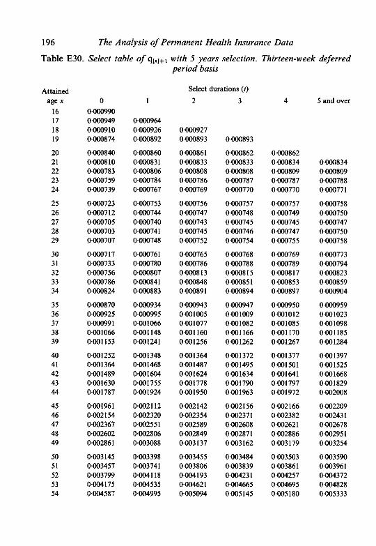
196 The Analysis of Permanent Health Insurance Data
Table E30. Select table of q,,,,, with 5 years selection. Thirreen-week deferred period basis
Attained age x
16 17 l8 19
20 21 22 23 24
25 26 27 28 29
30 31 32 33 34
35 36 37 38 39
40 41 42 43 44
45 46 47 48 49
50 51 52 53 54
Select duradons (I)
5 and over
0.000834 0.000809 0.000788 0000771
0.000758 0~000750 0.000747 0.000750 0.000758
0.000773 0.000794 0.000823 0.000859 0.000904
0.000959 0.001023 0.001098 0-001185 0.001284
0.001397 0.001525 0,001668 0.001829 OQLl2008
0002209 0.002431 0.002678 0.002951 0.003254
0-003590 0.003961 OW4372 0.004828 0.005333
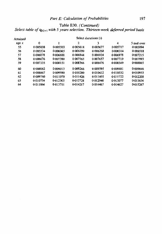
Part E: Calculalion of Probabilities 197
Table E30. (Continued) Select table of qlXl+, with 5 years selection. Thirteen-week deferredperiod basis
Attained age x
55 56 57 58 59
M)
61 62 63 64
Select durations ( I )
2 3 0.005618 0.005677 0.006199 0.006268 0.006844 0-006924 0.007563 0.007657 0.008366 0.008476
0.009266 0.009395 0.010280 0.010432 0.011426 0.011605 0.012728 0.012940 0.014217 0-014467
5 and over 0.005894 0.006518 0.007215 0.007993 0.008865
0.009846 0.010953 0.012208 0.013636 0.015267

198 The Analysis of Permanent Health Insurance Data
Table E31. Select table qf ia&,+, with 5 years selection: methods A and B: deferredperiod (d) 13 weeks. Thirreen-week deferred period basis
Age x
16 17 18 19
20 21 22 23 24
25 26 27 28 29
30 31 32 33 34
35 36 37 38 39
40 41 42 43 44
45 46 47 48 49
50 51 52 53 54
Duration t
3 4 5 and over B
0.001099 0.001191 0.001286 0001383
0.001485 0.001589 0.001696 0.001807 0.001921
0.002039 0-002162 0.002288 0002420 0.002557
0-002700 0.002851 0.003009 0.003171 0.003355
0.003546 0.003751 0003971 0~004210 0.004470
0-004755 0405068 0.005413 0.005795 0-006221
0.006698 0007233 0.007837 0-008521 0.009299
5 and over A
0.001099 0.001 191 0.001286 0.001383
0.001484 0001589 0001696 0.001807 0.001921
0.002039 0.002161 0-002288 0.002419 0002556
0-002699 0-002849 0.003007 0-003175 0.003353
0.003543 0.003747 0.003967 0.004205 0.004464
0.004747 0005058 0.005401 0.005782 0.006205
0.006677 0.007208 0.007806 0.008482 0-009251

Age x
Part E: Calculation of Probabilities
Table E3 1. (Continued) Select table of ia&+, with 5 years selection: methods A and B:
deferred period ( d ) I3 weeks. Thirteen-week deferred period basis
Duration t 0 I 2 3 4 5 and over 5 and aver
B A 0-W7813 0.010260 0.010234 0.010215 0.010200 0.010187 0-010127 0008612 0.011299 0.011266 0011241 0.011222 0.011206 0.011130 0.009536 0-012497 0.012456 0.012425 0.012400 0.012380 0.012282 0.010610 0.013888 0.013834 0.013794 0.013762 0.013736 0.013612 0-011863 0-015507 0.015438 0.015386 0.015345 0.015311 0.015151
0.013334 0.017403 0.017313 0017244 0~017190 0.017146 0.016938 0-015068 0.019633 0.019513 0.019423 0.019351 0.019292 0-019019 0.017123 0.022267 0022101 0.021985 0-021889 0.021811 0.021451 0.019571 0.025393 0.025177 0.025012 0.024882 0.024778 0.024297 0.022503 0.029120 0.028825 0.028600 0.028422 0.028279 0-027634
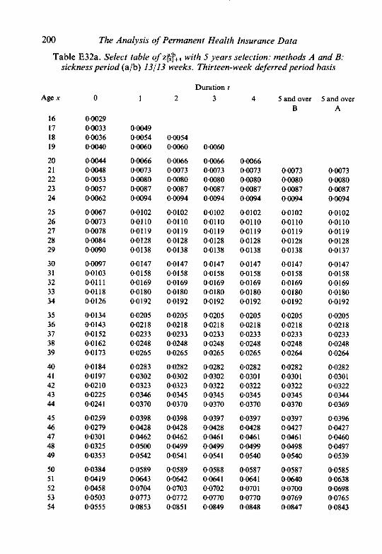
200 The Analysis of Permanent Health Insurance Data
Table E32a. Select table of z@+, with 5 years selection: methods A and B: sickness period (a/b) 13/13 weeks. Thirteen-week deferred period basis
Age x
16 17 18 19
20 21 22 23 24
25 26 27 28 29
30 31 32 33 34
35 36 37 38 39
40 41 42 43 44
45 46 47 48 49
50 51 52 53 54
5 and aver B
0.0073 0.0080 0.0087 0.0094
0.0102 0~0110 0~0119 0.0128 0.0138
0.0147 0.0158 0.0169 0.0180 0.0192
0.0205 0.0218 0.0233 0.0248 0.0264
0.0282 0-0301 0.0322 0.0345 0.0370
0.0397 0.0427 0.0461 0.0498 0.0540
0.0587 0.0640 0.0700 0.0769 0.0847
I and over A
0.0073 0.0080 0.0087 0.0094
0.0102 0.01 10 0.01 19 0-0128 0.0137
0.0147 0.0158 0-0169 0.0180 0.0192
0.0205 0.0218 0.0233 0.0248 0.0264
0.0282 0.0301 0.0322 0.0344 0.0369
0,0396 0.0427 0.0460 0.0497 0.0539
0.0585 0.0638 0.0698 0.0765 0.0843

Part E: Calculation of Probabilities 20 1
Table E32a. (Continued) Select table of zf$+, with 5 years selection: methods A and B:
sickness period (aib) 13/13 weeks. Thirteen-week deferredperiod basis
Age x 0
Duration r 2 3 5 and over 5 and over
B A
0.0937 0.0932 0.1041 01034 01161 0-1152 01301 0-1289 0.1464 0.1449
0.1656 0.1635 0-1881 0.1855 0.2148 0.2112 02464 0-2416 0.2840 0.2775

202 The Analpis of Permanent Health Insurance Data
Table E32b. Select table of z@+, with 5 years selection: mefhods A and B: sickness period (a/b) 26/26 weeks. Thirfeen-week deferred period basis
Duration r Age x
16 17 18 19
20 21 22 23 24
25 26 27 28 29
30 31 32 33 34
35 36 37 38 39
40 41 42 43 44
45 46 47 48 49
50 51 52 53 54
5 and over 5 and over

Age X
55 56 57 58 59
M) 61 62 63 64
Part E: Calcularion of Probabilities
Table E32b. (Continued) Select table of zf$+, with 5 years selection: methods A and B:
sickness period (a/b) 26/26 weeks. Thirteen-week deferred period basis
Duration 1
2 3 5 and over B
0.1102 0.1246 0.1414 0.1612 0-1846
0.2124 0.2455 0.2852 0.3330 0-3906
5 and over A
01095 0.1237 0,1403 0.1597 0.1827
0.2098 0.2420 0-2805 0.3265 0.3817

204 The Analysis of Permunent Health Insurance Data
Table E32c. Select table of zf$+, with 5 years selection: method.7 A and B: sickness period (aib) 52/52 weeks. Thirreen-week deferredperzod basis
Age x
16 17 18 19
20 21 22 23 24
25 26 27 28 29
30 31 32 33 34
35 36 37 38 39
40 41 42 43 44
45 46 47 48 49
50 51 52 53 54
0
0~0000 0~0000 0-0000 0.0000
0.0000 0.0000 0.0000 0.0000 0.0000
0-0000 0.0000 0.0000 0.0000 00000
0.0000 0-0000 0-0000 0.0000 0~0000
00000 00000 0.0000 00000 0~0000
0.0000 o-oooo 0.0000 0-0000 0.0000
0.0000 0-WOO 0.0000 0-0000 0~0000
o-oooo 0.0000 0~0000 00000 0.0000
Duration t 1 2 3 4 5 and ova
B
0.0036 0-0041 0.0047 0-0053
0.0059 0.0067 00075 0.0083 0.0093
0.0103 0.0115 0.0127 0-0141 0.0156
0-0172 0.0190 0.0210 0.023 1 00255
0.0282 0-031 1 0.0344 0.0380 0.0421
00467 0.0519 00577 00.544 0.0720
00807 0.0906 0. L022 0-1 156 0-1311
5 and over A
0.0036 00041 0.0047 00053
00059 0.0067 0-0075 0.0083 0-0093
0.0103 0.0115 0-0127 0.0141 0.0156
0-0172 0-0190 0.0209 00231 0.0255
0.0281 0031 1 0.0343 00380 0.0420
0.0466 0-0518 0.0576 0.0642 0.0718
0.0804 0.0903 0-1018 0-1150 0.1304

Age x
55 56 57 58 59
60 61 62 63 64
Part E: Calculation of Probabilities
Table E32c. (Continued) Select table of z@+, with 5 years selection: methods A and B:
sickness period (a/b) 52/52 weeks. Thirteen-week d<ferredperiod basis
Duration t
3
0.1498 01713 0.1968 02270 0.263 1
0.3063 0-3584 0.4215 0.4984 05924
5 and over B
0,1494 0.1708 0,1961 0.2260 0.2617
0.3045 0-3559 0.4181 0-4935 05856
5 and over A
0.1484 0.1696 0.1945 0.2239 0.2589
0,3007 0.3508 04111 0.4839 0-5721

206 The Analysis of Permanent Healih Insurance Data
Table E33a. Sickness rates z ( x . l 0 4 / a l l , x x 0 ) Thirteen-week deferredperiodhasis
Attained Entry age m agex 16 17 18 19 20 21 22 23 24 25 16 0.0000 17 0.0000 0.0000 18 0.0006 0-0000 0.0000 19 0.0018 0.0008 0.0OM) 0-0000
20 0.0030 0.0021 0-0009 0.0000 0.0000 21 0-0042 0.0035 0.0025 0.0010 0.0000 O~WOO 22 0.0055 @W49 0-M)40 0.0029 0.0012 0-0000 0.0000 23 0.0071 0.0065 0-0057 0-0046 0.0033 0-0013 0.0000 O~WOO 24 0-0087 0.0082 04075 0-0065 0.0054 0.0038 0-0015 0.0000 0.0000
25 0.0106 0-0101 0-0095 0.0086 0,0075 0-0062 0.0043 0-0018 0.0000 0.0000 26 0.0127 0.0122 0.0117 0.0109 0.0099 0-0086 0-0070 0.0049 0-0020 0-0000 27 0.0150 0-0146 0.0141 0.0134 0-0125 0.0114 04G99 0-0080 0.0056 0.0023 28 0.0177 0.0173 0.0168 0.0162 0.0154 00143 0.0130 0.0113 0-0091 00064 29 0.0206 0.0203 0.0198 0.0193 0-0185 0.0175 0.0163 0-0148 0.0128 0.0104
30 0-0239 0.0236 0.0232 0.0227 0.0220 0.0211 0-0200 0.0186 0.0168 0-0145 31 0.0277 0.0274 0.0270 0.0265 0.0259 00251 0.0240 0.0227 0.0211 0.0190 32 0.0318 0.0315 0.0312 0.0308 0.0302 00294 0.0285 0.0273 0.0258 0.0239 33 0.0365 0.0362 0.0359 00355 0.0350 0.0343 00334 0.0323 0.0309 0.0292 34 0.0417 0.0415 0.0412 0.0408 0.0403 0.0397 00389 0.0379 0.0366 0.0350
35 0.0476 0.0474 00471 0.0467 0.0463 00457 0.0450 0,0440 00429 0.0414 36 0.0541 0.0540 0.0537 00534 0.0530 0.0524 00517 0.0509 0.0498 0.0484 37 0.0615 0.0613 0.0611 0.0608 00604 0.0599 0.0593 00585 0.0575 0.0562 38 0.0698 0.0696 0.0694 0.0691 0.0688 0.0683 00677 0.0670 0.0661 00649 39 0.0791 0.0789 0.0787 0.0785 00781 0.0777 0.0772 0.0765 0.0756 0.0745
40 00895 0.0894 0.0892 0.0890 0.0887 0.0883 0.0878 0.0871 0.0863 0.0853 41 0.1013 0.1012 0-1010 0.1008 0.1005 0-1001 0.0996 0.0990 0.0983 00973 42 0-1145 0.1144 0.1142 0.1140 0.1138 0.1134 0.1130 0-1124 0.1117 0.1108 43 0.1295 0-1294 0.1292 0.1290 0-1288 0-1284 0.1280 0.1275 01268 0.1260 44 0.1464 0.1463 0-1461 0.1459 0.1457 0-1454 0.1450 0.1445 01439 0.1431
45 0-1655 0.1654 0.1653 0-1651 0.1649 0.1646 0-1642 0-1638 0.1632 0.1625 46 0.1872 0.1871 0-1870 0.1868 0.1866 0-1863 0.1860 0.1856 0-1850 0.1844 47 0-2119 0.2118 0-2117 0-2115 0.2113 0.2111 0-2108 0.2104 0.2099 0.2092 48 0.2400 0-2399 0-2398 0.2397 02395 0.2393 0.2390 0.2386 0-2381 0-2375 49 0-2722 0.2721 0.2720 0-2719 0.2717 0.2715 02712 0.2709 0.2704 0.2698
50 0.3091 0-3090 0.3089 0.3088 0-3086 0.3084 0.3082 0.3078 0-3074 0-3069 51 0-3515 0.3514 0.3514 0.3512 0-3511 0.3509 0.3506 0-3503 0.3499 0.3494 52 0~4005 0.4004 0-4003 0.4002 0.4000 03999 0.3996 0.3993 0.3989 0-3984 53 0.4571 0.4570 0.4569 0-4568 0.4567 0.4565 0-4563 0.4560 0.4556 0.4552 54 0.5229 0-5228 0.5227 0.5226 0-5225 0.5223 0.5221 0-5218 05215 0-5211

Part E: Calculation of Probabilities
Table E33a. fCorrrinued) Sickness rates z(x,lO4/aN,x -xo). Thirteen-week deferredperiod basis
Attained Entry age xo age X 16 17 18 19 20 21 22 23 24 25
55 0.5996 0.5995 0.5994 0.5993 0.5992 0.5991 0.5988 0-5986 0.5983 0.5978 56 0.6893 0.6893 0.6892 0.6891 0.6890 0.6888 0-6886 0.6884 06881 0.6877 57 0.7948 0.7948 0.7947 0.7946 0-7945 0.7943 0-7942 0.7939 0.7936 0.7932 58 0.9193 0.9192 0-9192 0.9191 0.9190 0-9188 0.9186 0.9184 0.9181 0-9178 59 1.0668 1.0667 1.0667 1-0666 1.0665 1.0664 1.0662 1.0660 1.0657 1.0654
60 1.2424 1.2424 1-2423 1.2422 1.2421 1-2420 1.2418 1.2416 1.2414 1.2410 61 1.4525 1-4524 1.4524 1.4523 1.4522 1.4521 1.4519 1.4517 1-4515 1.4511 62 1.7049 1.7049 1-7048 1.7048 1.7047 1.7045 1.7044 1.7042 1.7040 1 7037 63 2.0098 2.0098 2.0097 2.0097 2.0096 2-0095 2,0093 2.0091 2.0089 2.0086 64 2.3799 2.3799 2.3798 2.3798 2.3797 2.3796 2.3794 2.3792 2.3790 2.3787

208 The Analysis of Permanent Health Insurance Data
Table E33b. Sickness rafes z(x,l04/aN,x - X " ) . Thirteen-week deferredperiodbasis
Attained Entry age ao age x
26 27 28 29
30 31 32 33 34
35 36 37 38 39
40 41 42 43 44
45 46 47 48 49
50 51 52 53 54
55 56 57 58 59
60 61 62 63 64

Part E: Calculation of Probabilities
Table E33c. Sickness rates z(x,l04/aN,x - X & Thirteen-week deferredperiodbasis
Attained Entry age xo age x
36 37 38 39
40 41 42 43 44
45 46 47 48 49
50 51 52 53 54
55 56 57 58 59
60 61 62 63 64

210 The Analysis of Permanent Health Insurance Data
Table E33d. Sickness rates z(x,I04/all,x - xo). Thirteen-week deferredperiod basis
Attained Entry age xa age X
46 47 48 49
50 51 52 53 54
55 56 57 58 59
60 61 62 63 64
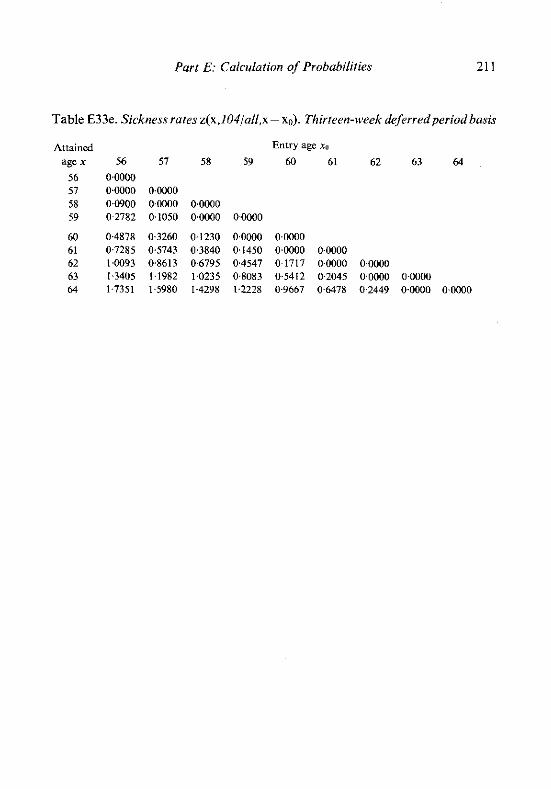
Part E: Calculation of Probabilities 21 1
Table E33e. Sickness rates z(x.I04/all,x- xo). Thirteen-week deferredperiodbasis
Attained Entry age xo age x 56 57 58 59 60 61 62 63 64
56 0.0000 57 0.0000 0.0000 58 0.0900 0-0000 0.0000 59 02782 0.1050 0.0000 0.0000

212 The Analysis of Permanent Health Insurance Data
Table E34. Select table of with 5 vears selection. Twenrv-six-week deferred
Attained age x
16 17 18 19
20 21 22 23 24
25 26 27 28 29
30 3 1 32 33 34
35 36 37 38 39
40 41 42 43 44
45 46 47 48 49
50 51 52 53 54
.. . pr idd basis
Select durations ( t )
1 2 3 5 and over
0000766 0-000731 0.000701 0000675
0.000653 0.000638 0.000627 0.000623 0.000624
0000633 0.000648 0-000671 0.000703 0.000743
0.000792 0000852 0000922 0.001004 0-001098
0001206 0.001329 0-001468 0.001623 0001798
0401992 0002208 0.002449 0.002715 0.003010
0-003336 0003697 0.004096 0-004536 0.005023

Part E: Calculation of Probabilities 213
Table E34. (Continued) Select table of qlXl+, with 5 years se/ecrion. Twenty-six-week deferredperiod basis
Attained Select duration5 (I)
age x 0 1 2 3 4 5 and over
55 0004870 0-005255 0-005350 0.005399 0405431 0.005561 56 0.005353 0.005797 OW5908 0-005965 0-006W3 0.006156 57 0.005880 0.006392 0.006524 0.006591 0.006635 0006815 58 0006456 0007048 0-007202 0.007281 0.007334 0407546 59 0.007084 0007770 0-007951 0008045 0.008101 0.008355

214 The Analysis of Permanent Health Insurance Data
Table E35a. Select table of ia&+, with 5 years selection: methods A and B: deferredperiod ( d ) 26 weeks. Twenty-six-week deferredperiod basis
Age x 0
Duration r 3
0-000196
0.000207 0000219 0.000232 0000246 0.000262
0000280 0.000299 0.000320 0-000343 0.000368
0000397 0~000428 0.000462 0~000500 0-000542
0.000589 0.000641 0-000699 0400764 0.000836
O.OW916 0-001007 0.001 108 0-001221 0.001349
0-001493 0.001655 0-001839 0.002046 0002281
0-002547 0002850 0.003194 0-003586 0.004034
5 and over B
0400219 0-000232 0.000246 0000262
0.000280 0000299 0.000320 0.000343 0-000368
0-000397 0400428 0-000462 0-000500 0-000542
0.000589 0400641 0.000699 0000763 0.000835
0.W0916 0.001006 0.001107 0.001221 0.001348
0-001492 0.001654 0001837 0.002044 0-002279
0.002544 0-002846 0.003 L90 0.003581 0.004027
5 and over A
0-000219 0.000232 0400246 0.000262
0000280 0.000299 0.000320 0000343 0.000368
0.000396 0.000428 0.000462 owJo500 0.000542
0-000589 0400641 0-000699 0.000763 0000835
0.0009l6 0.001006 0.001 107 0.001220 0.001347
0.001491 0-001652 0.001835 0-002041 0-002275
0.002539 0402840 0-003181 0403569 0004012

Part E: Calculation of Probabilities 215
Table E35a. (Continued) Select table of ia&+, with 5 years selection: methods A and B:
deferredperiod ( d ) 26 weeks. Twenty-six-week deferred period basis
Age x
55 56 57 58 59
60 61 62 63 64
5 and over B
0.004536 0.005118 0.005784 0.006547 0-007422
0.008427 0.009581 0.010907 0.012432 0-014185
5 and over A
OW4516 0.005092 0.005750 0.006502 0.007363
0.008347 0.009474 0.010764 0.012239 0.013923

216 The Analysis of Permanent Health Insurance Data
Table E35b. Select table of ia&+, with 5 years selection: methods A and B: deferredperiod ( d ) 52 weeks. Twent.v-sis-week deferred period basis
Age X
16 17 18 19
20 21 22 23 24
25 26 27 28 29
30 31 32 33 34
35 36 37 38 39
40 41 42 43 44
45 46 47 48 49
50 5 1 52 53 54
Duration r 1 2 3 4 5 and over
B
0.000082 0000088 0000095 0.000103
OOWlll 0~000121 00001 32 0,000144 0.0001 57
0.000171 0.000188 0.000206 0000227 0.000250
0000276 0000305 0.000338 0000375 0.000418
0.000465 0000519 0.000580 0.000650 0.000730
0000820 0.000924 0001042 0.001 178 0001334
0.001513 0001719 0.001957 0.002231 0.002549
5 and over A
0.000082 0.000088 0000095 0.000103
0000 l l l 0~000121 0000132 0.000144 0.000157
0000171 0.000188 0.000206 0000227 0.000250
0.000276 0000305 0.000338 0000375 0.000417
0.000465 0000519 0400580 0000650 0.000729
0000819 0000923 0001041 0.001176 0.001331
0.001510 0001715 0.001951 0002224 0.002539
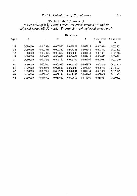
Age x
Part E: Calculation of Probabilities
Table E35b. iContinued) Select table of ia&+, with 5 years selection: methods A and B:
deferred period (d) 52 uveks. Twenty-six-week deferredperiod basis
Duration r
0 1 2 3 4 5 and over 5 and over B A
0.000000 0.002936 0-002927 0.002923 0.002919 0002916 0.002903 0000000 0-003369 0403357 0.003351 0003346 0.003342 0-003325 0000000 0-003872 0-003857 0.003848 0003842 0.003837 0.003814 0.000000 0.004458 0-004439 0.004427 0.004419 0-004412 0,004381 0~000000 0.005143 0005117 0-005102 0.005090 0-005081 0.005040
0000000 0005943 0-W5910 0005889 0005873 0.005860 0-005805 0.000000 0006880 0-006836 0.006808 0.006787 0006770 0.006694 0000000 0.007980 0.007921 0-007884 0.007854 0-007830 0.007727 0.000000 0009272 0-009194 0.009142 0-009102 0-009069 0.008928 0000000 0.010792 0.010687 0-010617 0.010561 0-010517 0010322

218 The Analysis of Permanent Health Insurance Dara
Table E36a. Select table of if$+, with 5 years selection: methods A and B: sickness period (a/b) 26/26 weeks. Twenty-six-week deferredperiod basis
Duration r 1 2 3 4 S and over
B
0-0033 0.0035 0.0038 0.0041
0.0044 00047 0.0051 0.0055 0.0059
0-0064 0.0070 0.0076 00083 0.0091
0-0100 0.01 10 0.0121 0-0133 0.0147
0.0162 0.0180 0.0200 00222 0.0247
00276 0.0309 0-0346 0.0388 0-0436
0-0491 0.0554 00627 0-0710 0.0805
5 and over A
0.0033 00035 0.0038 0-0041
0.0044 0.0047 0.005 1 0-0055 00059
0.0064 04il70 0-0076 0.0083 0,009 1
0~0100 0~0110 0.0121 0.0133 0.0147
0.0162 0.0180 0-0199 0.0222 0-0247
0.0276 00308 0.0345 0-0387 0.0435
0.0490 0.0553 0.0625 0.0708 00802

Parr E: Calculation of Probabilities 219
Table E36a. (Continued) Select table of zr$+, with 5 years selection: methods A and B:
sickness period (a/b) 26/26 weeks. Twenty-six-week deferred period basis
Duration t
Age x 0 I 2 3 4 5 and over 5 and over B A
55 0.0258 0.0921 0-0918 0.0917 0.0916 0.0915 0.091 1 56 00293 0-1049 0.1046 0.1044 0-1043 0.1042 0.1036 57 0.0334 0.1197 0-1194 0.1191 0.1189 0.1187 0.1181 58 0.0382 0.1369 0-1364 0,1361 0.1358 0.1356 0.1347 59 0.0437 0-1569 0.1562 0.1558 0.1554 0.1551 01539
60 0.0500 0.1800 0-1792 0.1786 0.1781 0.1777 0.1760 61 0-0574 0.2070 0.2058 0.2050 0.2044 0.2038 0-2016 62 0.0661 0.2384 0-2369 0.2357 0-2349 0.2342 0.231 1 63 0-0762 0.2751 0-2730 0.2715 0.2703 0,2693 0.2652 64 0-0879 03179 0.3151 0.3131 03115 0,3102 0.3044

220 The Analy.~;.~ of Permanent Health Insurance Data
Table E36b. Select sable o f z&!+, with 5 years selection: methods A and B: sicknessperiod (a,lb) 52/52 weeks. Twenty-six-week deferred period basis
Age x
16 17 18 19
20 21 22 23 24
25 26 27 28 29
30 31 32 33 34
35 36 37 38 39
40 4 1 42 43 44
45 46 47 48 49
50 51 52 53 54
Duration t
I 2 3 4 5 and ove~ B
0-0028 00030 0.0033 0.0036
0.0039 00043 0.0047 0005l 0.0057
0.0062 0.0069 0-0076 0.0084 0-0093
0.0103 0 0 l l 5 00128 00143 0.0160
0-0179 0.0201 0.0226 00255 0.0288
00326 0.0369 00419 0.0477 0 0 Y 3
0.0620 00708 0.08 11 0.0931 0.1070
5 and over A
00028 0.0030 0.0033 00036
0.0039 0.0043 04047 0-0051 0.0057
00062 0.0069 0.0076 0.0084 0-0093
0-0103 0.01 15 00128 0.0143 00160
0.0179 0~0201 00226 0.0255 00288
0.0326 00369 0.0419 0-0476 0.0542
0-0618 0.0707 0.0809 00928 01066
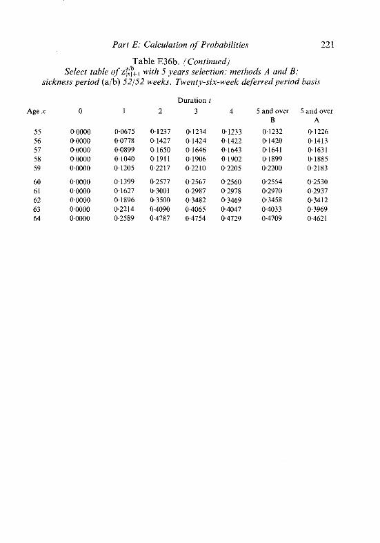
Part E: Calculation of Puohahilities 221
Table E36b. (Conrinuedj Select tahle of z$k, wilh 5 years selection: methods A and B:
sickness period (a/b) 52/52 weeks. Twenty-six-week deferredperiod hasir
Duration t
Age x 0 I 7 3 4 5 and over 5 and over B A
55 0.0000 0-0675 0-1237 0,1234 0.1233 0.1232 01226 56 00000 0-0778 0.1427 01424 0,1422 0.1420 0.1413 57 0.0000 0.0899 01650 01646 0,1643 0.1641 0-1631 58 0-0000 01040 0.1911 0-1906 0,1902 0,1899 0.1885 59 0-0000 01205 0-2217 0.2210 0.2205 02200 0.2183
60 0.0000 0,1399 0-2577 0-2567 0.2560 0.2554 02530 61 00000 01627 0.3001 02987 02978 0.2970 02937 62 0.0000 01896 03500 03482 0.3469 0.3458 0.3412 63 0-0000 0.2214 04090 04065 0.4047 0.4033 03969 64 0-0000 02589 0.4787 0.4754 0.4729 0.4709 0.4621

222 The Analysis of Permanent Health Insurance Dala
Table E37a. Sickness rates z(x,lO4/a/l,x-XO). Twenty-six-week deferred period basis
Attained Entry age xo age r
16 17 18 19
20 21 22 23 24
25 26 27 28 29
30 31 32 33 34
35 36 37 38 39
40 41 42 43 44
45 46 47 48 49
50 51 52 53 54

Part E: Calcularion of Probabilities
Table 37a. (Continued) Sickness rates z(x, I04/aN,x - xo). Twenry-six-week deferredperiod basis
Attained agex 16
55 0-4546 56 03305 57 0-6201 58 0.7262 59 0-8519
M) I.0012 61 1.1787 62 1.3902 63 1.6424 64 1.9439
Entry age xa
17 18 19 20 21 22 23 24 25
0.4546 0.4545 0.4544 0-4543 0.4542 0.4540 0.4539 0.4536 04534 05304 05304 0-5303 0.5302 0.5301 0-5299 0.5297 0-5295 0-5293 0.6200 0-6200 0.6199 0.6198 0.6197 0.6196 0.6194 0-6192 0.6190 0.7261 0.7261 0.7260 0.7259 0.7258 0.7257 0.7255 0.7253 0-7251 0.8518 0.8518 08517 0.8516 0.8515 0.8514 0.8513 0-8511 0.8509
1.0011 1.0011 1-0010 1.0009 10008 1.0007 1.0006 1-0004 1.0002 1,1786 1.1786 1.1785 1.1785 1,1784 1-1783 11781 1.1779 1-1777 1.3901 1.3901 1.3900 1.3899 1.3898 1-3897 1.3896 1.3894 1.3892 1,6424 1.6424 16423 1.6422 1.6421 1-6420 1.6419 1-6418 1.6416 1-9439 1.9438 1-9438 1.9437 1.9436 1-9435 1.9434 1-9432 1.9430

age X
26 27 28 29
30 31 32 33 34
35 36 37 38 39
40 41 42 43 44
45 46 47 48 49
50 51 52 53 54
55 56 57 58 59
60 61 62 63 M
224 The Analysis of Permanent Health Insurance Data
Table E37b. Sickness rates z(x, l04/al l .x-xo). Twenty-six-week deferred period basis
Attained Entry age xo 26 27 28 29 30 31 32 33 34 35

Part E: Calculation of Probabilities
Table E37c. Sickness rutes z(x,l04juN,x-xo). Twenty-sir-week deferredperiod basis
Attained Entry age xo age x
36 37 38 39
40 41 42 43 44
45 46 47 48 49
50 51 52 53 54
55 56 57 58 59
60 61 62 63 64

226 The Analysis of Permanent Health Insurance Data
Table E37d. Sickness rates z(x,lO4/all,x-xo). Twenty-six-week deferred period basis
Attained Entry age xo agex 46 47 48 49 50 51 52 53 54 55
46 0.0000 47 0.0000 0 . m 48 0.0174 0.0000 0.0000 49 0.0520 0.0199 0-0000 0.0000
50 0.0888 04600 0.0229 0.0000 0.0000 51 0,1295 0.1026 0.0692 0.0264 00000 0.0000 52 0.1755 0.1500 0.1188 0-0800 0.0305 0.0000 0-0000 53 0.2278 0.2037 0.1741 0.1377 0.0927 00353 0~0000 0.0000 54 0.2878 0.2649 0.2368 0-2023 0.IMH) 0.1076 0-0409 0.0000 0~0000
55 0.3572 0.3353 0-3086 0.2758 0.2356 0.1863 0.1251 0.0475 0-0000 0~0000 56 0.4376 0.4168 0-3913 0.3601 0.3218 0.2749 0.2172 01458 0.0553 0.0000 57 0.5315 0.5117 0.4873 0.4576 0.4210 0-3762 0.3212 0.2537 0-1701 0.0644 58 0.6415 0-6225 0.5993 0.5708 0-5359 0.4931 0,4406 0.3761 0.2969 0-1989 59 0.7709 0.7527 07305 0.7032 0.6698 0.6289 0.5786 0.5169 0.4412 0.3481
60 0.9235 0.9061 0.8848 0.8587 0.8267 0.7874 0.7393 0.6802 06076 0.5185 61 1.1041 1.0875 1.0670 1.0419 1.0112 0.9735 0-9273 0-8706 0,8010 07155 62 1.3185 1.3025 1.2828 1.2587 1.2292 1,1930 1-1485 1.0940 1.0271 0.9450 63 1.5735 1.5580 1.5391 1-5159 1.4875 14526 1-4099 1.3574 1-2930 1.2140 M 1.8774 1.8625 1.8443 1.8219 1.7945 1.7609 1.7197 1.6692 1.6071 1-5309
Table E37e. Sickness rates z(x,l04/all,x-Q). Twenty-six-week deferred period basis
Attained age X
56 57 58 59
Entry age xo
59 60 61 62 63 M

CMIR 12 (1991) 227-252
PART F: CALCULATION O F MONETARY FUNCTIONS
SUMMARY
In this Part the calculation of monetary functions, mainly annuity values of various types, is discussed. First, in Section 1, an example of the calculation of 'exact' annuity values using the detailed methods of Part E, is shown. In Sections 2 and 3 the calculation of corresponding annuity values using 5 and z functions is considered, and in Section 4 the use of select tables of z functions and the size of error introduced by their use are discussed. Then in Section 5 the values of 'current claim annuities'are described, preparatory in Section 6 to describing two ways of calculating the corresponding annuity values using inception rates, of types (a) and (b), and appropriate average values of current claim annuities. In Section 7 the use of select tables of inception rates is considered. In Section 8 specimen premium rates are shown, and Section 9 contains some concluding observations.
1. ANNUITIES PAYABLE IN A GIVEN STATUS-TOTAL SICKNESS ANNUITIES
1.1 In Section 7 of Part D it was described how the expected present values of annuities payable while in a given status could be calculated to a high degree of accuracy (within the approximations inherent in the whole calculation method); we describe these as the 'exact' values. The expected present values of annuities payable monthly in advance provided that the life is in a particular status at the due date can be calculated exactly. The expected present values of annuities payable continuously can be calculated approximately, to a high degree of accuracy, by the trapezium rule applied over steps of A of a year. Continuous annuities approximate closely to annuities payable in strict proportion to the duration of sickness, or to the duration of sickness beyond any deferred period.
It is convenient to calculate the expected present values of annuities for each term of years commencing at a given starting age. We revert, for the purposes of example, to the life who is in the healthy state at age 30, and we calculate annuities for terms of 1 to 35 years, on the I week deferred period basis. Table F1 shows the expected present values of annuities payable continuously in each status and Table F2 shows the expected present values of annuities payable monthly in advance provided that the life is in the given status on the due date. Results are shown for the followine statuses: healthv; sick (all sickness ~eriods): , . living (healthy plus sick); and sick &ring specified sickness periods. 1f we were to include the status dead and sum theannuities payable in various statuses to give
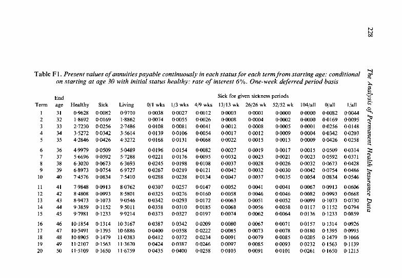
Y Table F1. Present values of annuities payable continuously in each statusfor each term from starting age: conditional on starring at age 30 with initial status healthy: rare of interest 6%. One-week deferredperiod basis
End Sick far given sickness pcriods $ 'S-
Tern age Healthy Sick Living O/l wks 113 wks 419 wks 13/13 wk 26/26 wk 52/52 wk 104/all O / d l l /d l %
1 31 0.9628 0.0082 0.9710 00038 0.0027 0.0012 0.0003 0.0001 0.0000 0.0000 0.0082 00044 2 32 18692 00169 1-8862 00074 00055 0-0024 0-WO8 0.0004 0-0002 0-0000 0-0169 00095 2 3 33 2.7230 0.0256 2.7486 00108 0.0081 0.0041 0-0012 00008 0.0005 0-0001 0-0256 00148 3 4 34 3.5272 0.0342 3.5614 00139 0.0106 0.0054 0.0017 0.0012 0.0009 0.0004 0.0342 0.0203 5 35 4.2846 0.0426 4.3272 0.0168 0.0131 0.0068 0.0022 0.0015 0.0013 0.0009 00426 0.0258
6 36 4.9979 0.0509 5.0489 0.0196 0.0154 0.0082 0.0027 0.0019 0.0017 0.0015 00509 0-0314 5 7 37 56696 0.0592 5.7288 0.0221 0.0176 0.0095 0.0032 0.0023 0.0021 0.0023 00592 0-0371 E 8 38 63020 0-0673 63693 0-0245 0-0198 0-0108 0-0037 0-0028 00026 0-0032 0-0673 0.0428 3 9 39 6.8973 0.0754 6.9727 0.0267 0.0219 0.0121 0.0042 0.0032 0.0030 00?42 0-0754 0-0486 k
10 40 74576 0.0834 7.5410 0.0288 0.0238 0.0134 0.0047 0.0037 00035 0.0054 0.0834 0.0546
11 41 7.9848 0.0913 8.0762 0.0307 0.0257 0.0147 0.0052 0.0041 0.0041 0.0067 04913 0.0606 12 42 8.4808 0.0993 8.5801 0.0325 0.0276 0.0160 0.0058 0.0046 0.0046 0.0082 0.0993 0.0668 R 13 43 8-9473 0-1073 90546 0-0342 0-0293 00172 0-0063 0-0051 0-0052 0-0099 0-1073 00730 2 14 44 9.3859 0.1152 95011 0.0358 0.0310 00185 0.0068 0.0056 0.0058 0.0117 0.1152 0.0794 g 15 45 9-7981 0.1233 9-9214 0.0373 0-0327 00197 0.0074 0.0062 0.0064 0.0136 0.1233 0.0859
16 46 10.1854 0.1314 10.3167 0.0387 0.0342 0.0209 0.0080 0.0067 0.0071 0.0157 01314 0.0926 17 47 10-5491 0-1395 10-6886 0-0400 0-0358 0-0222 0-0085 00073 0-0078 0-0180 01395 0-0995 18 48 104905 0.1479 11.0383 0.0412 0.0372 0.0234 04091 0.0079 0.0085 0.0205 0.1479 0.1066 19 49 11.2107 0.1563 11.3670 0.0424 0.0387 0.0246 0.0097 0.0085 0.0093 00232 01563 0.1139 20 50 11-5109 0-1650 11-6759 00435 00400 0.0258 00103 0.0091 0.0101 0.0261 0,1650 0.1215

Table F1 (Continued)
End Term age
21 51 22 52 23 53 24 54 25 55
26 56 27 57 28 58 29 59 30 60
31 61 32 62 33 63 34 64 35 65
Sick
0-1738 0.1829 01923 0-2020 0,2121
0.2225 02334 0.2449 0.2568 0-2694
0.2827 0.2967 0.3115 0.3273 03439
Living
11.9660 12.2384 12-4939 12-7336 12.9583
13.1687 13.3656 13.5498 13-7218 13.8823
14.0319 141712 14.3006 14.4206 14.5318
O/l wks
0.0445 0-0455 0-0464 0.0473 0.0481
0-0489 0.0496 0.0503 0-0510 04517
0.0523 0-0529 0.0534 0-0540 0.0545
113 wks
0.0414 0-0427 0.0440 00452 00464
0-0476 0.0487 00499 0-0510 0.0521
0-0532 0.0542 04553 0-0563 0.0573
419 wks
0.0270 00282 0.0294 04306 0-0318
0.0330 0.0342 0-0354 0.0367 04379
00392 0.0405 0-0418 0.0431 0.0444
Sick for given sickness periods
13/13 wk 26/26 wk 52/52 wk
0-0110 0-W98 0.0109 0.0116 0.0105 0.0118 0.0123 0.0113 00128 0.0129 0-0120 00138 00136 0.0128 0.0149
00144 0.0137 0.0160 0.0151 0.0146 0.0173 0.0159 0.0155 0.0186 0.0166 0.0165 0-0200 0-0175 0-0175 0.0214
0.0183 0.0186 04230 0.0192 0.0197 0-0247 0-0201 0.0210 0.0265 0-0210 0.0222 0.0285 00220 0-0236 0.0305
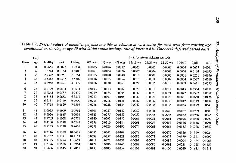
Y Table F2. Presenf values of annuities payable monthly in advance in each status for each term from starting axe: $- conditional an starting at age 30 with initial status healthy: rate of interest 6%. One-week deferredperiod basis L
2
Term I 2 3 4 5
6 7 8 9
10
I1 I2 I3 14 I5
I 6 17 18 19 20
End age
31 32 33 34 35
36 37 38 39 40
41 42 43 44 45
46 47 48 49 50
Healthy
0.9657 1.8744 27303 3-5365 4.2958
5-0109 5.6843 6.3183 69151 7.4768
80053 85026 8.9703 9-4100 9.8233
10.2116 10.5762 10.9185 1 1 -2396 115406
Sick 0.0077 0.0164 0.025 1 0-0337 0.0421
0-0504 0.0587 0.0668 0-0749 0.0829
0.0909 0.0988 0.1068 0-1148 01228
0.1309 01391 0,1474 0.1558 0-1645
Living
09734 1.8908 2.7554 3.5702 4-3379
5-0614 5.7430 63851 6.9900 7-5597
8.0962 8.6014 9.0771 9.5248 99461
10.3425 107153 11.0659 113954 11.7051
011 wks 0-0035 0.0071 00105 0.0136 001 h6
0.0193 0-0219 0.0243 0.0265 0-0286
0.0305 00323 0.0340 0.0356 0.0371
0.0385 0.0398 0-041 1 0.0422 0.0433
113 wks 0.0026 0-0054 0.0080 OOl05 0.0130
0.0153 0-0175 0-0197 0.0218 0.0238
0.0257 0-0275 0-0293 0.0310 0.0326
0-0342 0.0357 0-0372 0.0386 0.0400
419 wks
0.0012 0-0026 0.0040 0.0054 0.0067
0.0081 O.MW4 00108 0.0121 0.0134
0.0147 0.0159 0-0172 0.0184 0.0197
0-0209 0.0221 0.0233 0-0245 0.0257
Sick for given sickness periods
13/13 wk 26/26 wk 52/52 wk
0.0003 0~0001 0-0000 0,0007 0.0004 0.0002 0-0012 0.0008 0.0005 0.0017 00011 0.0009 0.0022 04015 00013
0.0027 0-0019 00017 0.0032 0.0023 04021 0.0037 0.0028 0,0026 0.0042 00032 0.0030 0.0047 0,0036 0-0035
00052 0-0041 0.0040 0.0057 0.0046 00046 0.0063 0.0051 0.0051 0-0068 0-0056 0.0057 0.0074 0-0061 0-0064
0.0079 0.0067 0.0070 0.0085 00073 0-0077 0.0091 0.0079 0.0085 0-0097 0.0085 0.0092 0-0103 0-0091 0.0100

Table F2 (Continued)
End Term age
21 51 22 52 23 53 24 54 25 55
26 56 27 57 28 58 29 59 30 60
31 61 32 62 33 63 34 64 35 65
Healthy
11.8227 12.0867 12.3336 12.5642 12.7794
12.9800 13.1666 13-3398 13-5004 13.6488
13-7856 13.9113 14.0263 14-1311 14,2259
Sick
0.1733 0-1824 0.1918 0.2014 0.2115
02219 0.2328 0-2442 02562 0.2687
0-2820 02960 0.3108 03264 0.3431
Living
11.9960 12.2691 12.5253 12.7657 12.9909
13-2019 13.3994 13.5840 13-7566 13.9175
14.0676 14-2073 14.3371 14-4575 14.5690
011 wks
0,0443 0-0453 0.0462 0.0471 0.0479
0-0487 0.0495 0.0502 0-0508 0.0515
0.0521 0-0527 0.0533 0-0538 0.0543
113 wks
0.0413 0-0426 0-0439 0.0451 0.0464
0-0475 0.0487 0.0498 0-0509 0.0520
0.0531 0-0542 0.0552 0-0563 0.0573
419 wks
0.0269 0-0281 0-0293 0.0305 0.0317
0-0329 0.0341 0.0354 0-0366 0.0379
0.0391 0-0404 0.0417 0-0430 0.0444
Sick for given sickness periods
13/13 wk 26/26 wk 52/52 wk
0.0109 04098 0.0109 0-0116 0-0105 0-01 18 0-0122 0-0112 0-0128 0.0129 0.0120 0.0138 0.0136 0.0128 0.0149
0-0143 0.0136 00160 0-0151 0-0145 00172 0.0158 0.0154 0.0185 0.0166 0.0164 0-0199 0.0174 0.0175 0.0214
0.0183 0.0185 0.0230 0-0191 0-0197 0-0246 0.0200 0,0209 0.0265 0-0210 0.0222 0.0284 0.0219 0.0235 0.0305

232 The Analysis of Permanent Health Insurance Data
the value of an annuity payable in any status, this would equal the present value of an annuity certain; such a calculation has been carried out and it provides a useful check on the calculation method.
In practice continuous annuities are applicable to benefits payable during periods of sickness, and annuities payable monthly in advance are applicable to premiums, which are normally paid while not claiming, i.e. either healthy or sick but within the deferred period.
2. APPROXIMATE CALCULATION OF ANNUITY VALUES USING FUNCTIONS
2.1 The annuity values discussed in Section 1 have been described as calculated exactlv. but usine calculation stem of &of a vear. Calculation with smaller stem. ~ -~~ ~ ~- , , U .." , . , which would provide any desired greater accuracy, would be possible, but not computationally worth while. We now turn to a series of methods for obtaining present values of annuities by simpler approximate calculations, and we discuss the degree of approximation involved.
2.2 We first consider formulae using the functions defined in Section 6.1 of Part D, which are discussed further in Section 3 of Part E, and for which specimen values are shown in Table E16. We also need the life table discussed in Section 4 of Part E; the values of l,, for this are shown in Table E17.
We start with the calculation of the present value of an annuity payable continuously while alive to a life who was healthy at age xa for a maximum term of n years, i.e. to a maximum age of xo+n years. In accordance with the notation introduced in Section 7.2 of Part D we give this the symbol
- X L a,,,
and we calculate it using the approximate formula
For the exact calculations above we have used the same trapezium rule but with steps of of a year.
The expected present value of an annuity payable continuously while sick, during sickness period ajb, conditional on being healthy at age X D , can be denoted by the function on the left of the approximation below, and calculated by the expression on the right.

Parr F: Calculation o/'Monetarj Functions 233
Note that, for symmetry, we show the first term in the calculation as (xo,a/h)/52, but in practice the value of this is zero, since it is assumed that all
those at no are healthy. The expected present value of an annuity payable continuously during all
sickness periods can be calculated as the summation of the appropriate annuities payable during each sickness period:
where the summation is over all relevant periods. The expected present value of an annuity payable whilst healthy can be
calculated by subtraction of the annuity payable while sick from the annuity payable while alive as:
2.3 Extensive calculations using these approximations were made. The method of calculating the annuities while living, a&, is satisfactory, producing errors, as compared with the more exact method, of no more than 3 parts in 10,000. The formula for sickness annuities. Z4sp', was found to be unsatisfactory. The problem arises in the first year. For example, for sickness period 011 weeks, the value of at the start of the first year is zero, but the average value of is nearly the same as the valueat theend of the first year. For a term of one year, therefore, the calculated sickness annuities fall substantially short of the exact values, by as much as 50%; the same absolute error persists for longer durations.
Rather than make special adjustments for the first year it seems better to use the sickness rates, the z functions as described in Section 3.
2.4 Annuities payable monthly in advance can he calculated using approxima- tions such as
and
Calculations using these formula show that the approximation for aet2' is

234 The Analysis of Permanent Health Insurance Data
just as good as for the continuous annuity, and that the approximation for U(=P~('~' is just as bad as that for riE:"'b'.
This shows, however, that the adjustment to convert from continuous to monthly payments is satisfactory.
3. APPROXIUATECALCULATION OF ANNUITY VALUES USING MANCHESTER-UNITY-STYLE SICKNESS RATES
3.1 Rather than use the C functions used in Section 2 we can carry out similar calculations using the sickness rates z . The functions are available for integral ages, whereas the z functions apply over a year of age: (X, X + l), (X+ 1, X + 2). etc. The formulae required are therefore slightly different.
3.2 Again we start with the calculation of the expected present value of an annuity payable while alive to a life who is healthy at age XO, for a maximum term of n years, i.e. to a maximum age of xo+n years. We can calculate this using the approximate formula
The expected present value of an annuity payable continuously while sick, during sickness period alb, conditional on being healthy at age xo, can be calculated approximately by the familiar formula
It will be seen that this is equivalent to the traditional 'Manchester-Unity' type of formula.
As before, the expected present value of an annuity payable continuously in all sickness periods can be calculated as the sum of the appropriate annuities payable during each sickness period, using formula (3).
The expected present value of an annuity payable whilst healthy can be calculated as before by subtraction of the annuity payable while sick from the annuity payable while living, using formula (4).
3.3 Annuities payable monthly in advance can be calculated using formula (6) for the annuity payable whilst living, and by

Parr F: Calculation of Monetary Functions 235
for the annuity payable during sickness period a/b. The term involving the average of two z's is a substitute for the value of at the terminal age of annuity; i.e. the adjustment is the same as in formula (7). At the end of a table the value of z(xn+n+ l,a/h) may not be available. In that case the approximation given by extrapolation: 2z(xo+n,a/b) -z(xo+n - l ,a/b) could be used instead.
Note that all the above are conditional on being healthy at age xn, and are calculated using the full table of sickness rates conditional on that entry age.
. .XL(12) 3.4 Extensive calculations show that the approximations for ZEL, and a,:, are only a little less accurate than those derived from the similar, but slightly different, formula (1). The errors are generally very small, but at high ages of entry rise to nearly 1 part per 1,000.
The values of ET^' are also very close to the exact values, being generally less than 1 part in 1,000 different from the exact value, and often very much closer. The exceptions occur for short duration and higher sickness periods, where the percentage errors approach 2% at the maximum; the absolute values, however, are very small, and the errors are always less than 0.001 in the annuity value per unit annual benefit.
The values of a ~ ~ ~ " ' * ' calculated using formula (l l) are a little less accurate than those of the corresponding continuous annuities, with errors generally less than 1 part in 1,000, except for the cases where the continuous annuity is less accurate, and for sickness period Oil week, where the error may be as large as 1 % (the approximation being too high) at short durations.
4. APPROXIMATE CALCULATION OF ANNUITY VALUES USING SELECT TABLES OF SICKNESS RATES
4.1 Instead of using the full set of tables of sickness rates as discussed in Section 3, we can alternatively make use of the select tables of sickness rates constructed in Section 9 of Part E. In the specimen calculations below we assume a 5-year select period, both for the life table and for the sickness rates; we have used the select tablecalculated using Methods A and Bof Section 9 of Part E. One must not expect this method to be satisfactory for calculating the values of annuities payable during sickness period 104/all, for the reason already explained in Section 9 of Part E.
The formulae exactly parallel those of Section 3, except that the functions are picked from the appropriate select table.
Thus we have approximately
where

236
and
The Analysis of Permanent Health Insurance Data
4.2 Calculations using this method show very satisfactory results. Values of 6:'-- have about the same proportionate error as those calculated using formula (8). but in the other direction, being slightly lower than the exact values rather than slightly higher.
Values of ri2'P' using Method A are slightly lower than those using formula (101. i.e. z's with an unlimited select oeriod. and those ushe Method B are higher. sin& formula (10) gives results a lhtle higher than the exact values, eth hod A gives results that are in some cases closer to the exact values than those from formula (10), whereas the results on Method B are always further away from the exact values, the error sometimes being up to 2% too high.
As already noted, a short select period table is unsatisfactory for calculating values for 104/all (or for any unlimited period contained within 104/all, e.g. 156/all), and is also unsatisfactory for any longer sickness period that includes this sickness period. For example, for sickness period ljall the results using Method A with a 5-year select period for 104/all would be up to 5% too high, and using Method B would be up to 20% too low.
5. VALUES OF CURRENT CLAIM ANNUITIES
5.1 We now consider "current claim annuities", i.e. annuities payable only during the current period of sickness, commencing when someone is already sick. We distinguish these from "future claim annuities", i.e. annuities payable during future periods of sickness, either to someone who is at present healthy, for whom the current claim annuity value is zero, o r to someone who is at present sick, but in respect of future sickness periods, not the current one.
Current claim annuities have already been introduced in Section 7 of Part D. They can be readily calculated. We first introduce the notation n(x,zi,zz) to represent the probability that an individual currently aged X and sick with exact duration z, conJinues while remaining sick to exact duration zz (z2>21) (the same as =,-,,pSI ). We have already introduced the notation K,,= in Section 10 of Part E to represent the probability that a life who has just become sick at age X
continues while sick to duration z, so that we can treat n,, as an abbreviation for n(x,O,z).

Part F: Culculution of Monetary Functions 237
5.2 We can now calculate the expected present value of an annuity payable continuously to someone who is currently aged X and sick with exact duration of sickness 2, payable so long as he remains sick, for a maximum duration of n, which has been defined in Section 7 of Part D as
- p -2' a
An exact expression for this is given by
where v is the usual discounting factor. It is possible to calculate this function as accurately as one likes by a number of
methods, usually requiring successive approximation. For example, one can calculate values of n(x,z,z+i) from the formula
and calculate the integral in the formula by an approximate integration formula such as the trapezium rule or Simpson's rule, each value being calculated to any desired accuracy by reducing the step size until successive approximations are close enough together. This method can be used for any required value oft . One can then calculate the integral
also by approximate integration, using the same, or a different approximation method, and the same or a different step size. It may be convenient to use the same step ske in the two approximations and to combine the process to calculate values of 6::. ,for a given combination of X and z and for various values of n, e.g. n = 1 , 2 , 3 . . . up to X + n = 65 say, all in the same sequence of approximations.
5.3 An alternative method, which is consistent with the calculations in Part E and in the earlier section of this Part is to calculate values of n(x,z,z + t ) by the recursive approximate formula:
with n(,:,:, = 1, and steps of h = of a year, and then to calculate 5::. , using the trapezium rule, also using steps of h = & of a year:
h " : h - , h riz::, = - + 1 hod n(x,z,z + jh) + - l ; " n(x,z,z + n)
2 ,=, 2 (19)

N W m
Table F3. Present ualues of continuous current claim annuities o f l Der vear ceasing at age 65: rate of interest 6%. 2 . 2
One-week deferred period basis Duration in weeks

Table F3 (Continued) Duration in weeks
Term
25 24 23 22 21
20 19 18 17 16
I5 14 13 12 I 1
10 9 8 7 6
5 4 3 2 I

240 The A~~alys is of Permanent Health Insurance Data
5.4 Table F3 shows approximate values of current claim annuities, payable continuously, at 6% interest, ceasing at age 65, for integral values of X from 16 to 64, and for values of z of 0, 1,4, 13, 26, 52 and 104 weeks calculated using the method just described. The values of these annuities have also been calculated using the more exact method described above. In general the approximate method produces values a little lower than the exact method. For z=O, i.e. annuities starting immediately a period of sickness starts, the error is as much as 4%, but for higher values of z the error is much smaller, being no more than about 0.5% for z= 1 week, and much less than this for high values of z. The error is greater at those durations of sickness when the recovery rates change rapidly with duration.
6. APPROXIMATE CALCULATION OF ANNUITY VALUES USING INCEPTION
RATES AND VALUES OF CURRENT CLAIM ANNUITIES
6.1 An alternative approach to the calculation of the expected present values of payments during sickness is by the use of inception rates and current claim annuity values. The difference between this method and the sickness rate method can be demonstrated in Figures F1_ F2 and F3. All of these use the same format as Figure El . They relate to a life who is healthy at age X" at point A, and to a benefit that commences after a 13-week deferred period. The duration of the policy is restricted in the figures to four years.
In all three figures the whole shaded area represents the region within which sickness benefit may he payable. In Figure F1 this is subdivided into mainly rectangular regions by horizontal and vertical lines. The horizontal lines represent years of age passed through, and the vertical lines represent different sickness durations passed through. Sickness periods 13/13, 26/26, 52/52 and 104/all are represented. To each rectangle there is a corresponding z(x,a/b), and the present value of sickness benefit is calculated first by multiplying these z(x,a/b) functions by an appropriate ratio L(x)ll(xo) and a discount factor, then by summing in columns to give the values of sickness benefit payable during a particular sickness period, and then by summing across sickness periods.
A second approach is shown in Figure F2. The shaded area is subdivided into diagonal stripes. Once a claim commences by the period of sickness passing across the 13-week claim inception boundary, the line representing this period of sickness remains within a single diagonal stripe until the life either recovers, dies or reaches the end of the period of cover, which in this case is age q + 4 . The inception rates of type (a) , ia(x,d) discussed in Section 5 of Part E, represent the proportion of lives among the L , survivors who cross the line for duration d between ages X and X+ l at each age, and the current claim annuities, commencing at duration d. for an appropriate average age, represent the values of benefit within each diagonal stripe.

Part F: Calculation of Monetary Functions 24 1
Dead Healthy Sick Dead from from
Healthy Sick
% A ..c Duration of sickness
rr-r---r-------- *ge h w 1 2 6 w 152w
Figure FI. Calculating sickness benefit using sickness rates
It can be noted that the stripes are not of equal width. The top stripe is only 391 52 or 3/4 of a year wide. This occurs because a life who is healthy at age X,, cannot reach 13 weeks of sickness until at least age no+ 13/52. With a 26-week deferred period the top stripe would only be half the width of the lower ones; for a 52-week deferred period the top stripe would disappear to nothing, and for longer deferred periods the second or lower stripes would also be affected.
A third way of subdividing the shaded region is shown in Figure F3, in which the diagonal lines start at the integral ages on the vertical line representing healthy. In this case the higher stripes are all the same width, representing one year, and the lowest one is narrower, in this case only 314 of a year wide. For this partitioning one uses the claim inception rates of type (h), ib(x,d) discussed in Section 5 of Part E.
This third approach may be useful when calculating l-year cover sickness benefit for group PHI policies, where the cover granted is for sickness that commences in the year of age (xo,xo + 1) and continues for a duration of at least d, the claim annuity then being payable up to some maximum age.

242 The Analysis of Permanent Health Insurance Data
Dead Heolthy Sick Dead from from
Healthy Sick A + Duration of sickness
Figure FZ. Calculating sickness benefit using inception rates of type (0).
6.2 In Section 5 of Part D it was shown how the inception rates ia(x,d) were derived from the numbers of claim inceptions ca(x,d). The latter can be reconstructed from the former by the formula
and the alternative claim inceptions cb(x,d) can be approximated by
cb(x,d) = (1 - d)ia(x,d) . L, + d . ia(x + 1 ,d ) . L,,, (21)
It will be noted that for the partitioning in Figure F2, appropriate to the inception rates of type (a) the line representing deferred period d(13 weeks in the figure) is subdivided into intervals (xo+d,xo+ l ) , (xo + 1,x0+2), (xo+2,xo+ 3), (xo+ 3,x0+ 4) , whereas in Figure F3, appropriate to inception rateof type(b), the corresponding line is subdivided into intervals ( x o + d , x o + l + d ) , (xo+l+d,xo+2+d) , (xo+2+d,xa+3+d),(xo+3+d,x0+4). These can be

Part F: Calculation of Monetary Functions 243
Dead Healthy Sick Dead from
Heolthv from Sick . - . . . . .
A -m Duration of sickness xo "LW-------- - F - - - v -
Figure F3. Calculating sickness benefit using inception rates of type (b) .
combined, as shown in Figure F4 where the subdivision is (xO+d,xo+ l), (xo+ I,xo+ 1 +d), (xO+ 1 +d,x0+2), etc. with sections alternatively dand (1 - d ) wide, and labelled alternately '2' and 'l'.
6.3 We define two types of average annuity value, each being the average of current claim annuities, commencing at duration d, but the first averaging annuities commencing between ages x and x+d, and the second averaging annuities commencing between ages x + d and x + l , in both cases for integral values of X, and ceasing at age x+n. We define these for 0 < d < 52 weeks as
and

Table F4. Average values of continuous current claim annuities of I per year, payahle while sick commencing at given k' age andgiven duration of sickness and ceasing at age 65: types ( I ) and (2 ) : rate of interest 6%. One-week deferred
period basis
Duration 0 weeks l wcek 4 weeks 13 weeks 26 weeks 52 weeks 104 weeks U

Table F4 (Continued)
0 weeks l week
(1) (2) (1) (2) 00626 0-0 0.1079 0.1120 0.0673 0.0 0.1163 01208 0.0726 0 0 01254 01304 0-0784 0.0 0.1354 0.1408 00849 0.0 0.1463 0.1522
0-0919 0-0 0-1582 0-1645 0.0997 0.0 0.1710 0.1778 0.1081 0.0 0.1848 0-1921 0.1173 0-0 0-1996 0-2074 01272 0.0 0.2154 0.2237
0.1378 0 0 0.2321 0.2408 0,1491 0.0 0.2496 02585 0.1609 0.0 0.2676 0.2768 01732 0 0 0.2860 0.2951 0.1855 0 0 03042 0-3131
0-1977 0.0 0.3219 0.3301 0.2091 0.0 0.3381 0.3453 0.2191 0 0 0-3519 0-3574 0.2267 0.0 0.3621 0.3651 0-2308 0-0 0-3669 0-3663
02296 0.0 0.3643 0.3588 0.2209 0-0 0-3513 03392 02017 0-0 0-3243 0.3031 0.1672 0.0 0.2780 02437 0-1006 0-0 0.2035 0.1377
13 weeks
(1) (21 1.2318 1.2610 1-2905 1-3205 1.3508 1.3815 1.4125 1.4437 1-4752 1-5068
1.5385 1.5701 l6018 16332 16644 1-6951
reeks 52 weeks
(2) (1) (2) 2.7466 4-5319 0-0 2.8329 4.6153 0.0 29184 4.6943 0.0 30023 47678 0-0 30837 4.8344 0.0
3-1616 44928 0.0 3.2346 4.9414 0.0 3.3014 4.9783 0.0 3.3603 5.0015 0.0 3.4092 5-0087 0-0
3-4460 49974 0.0 3.4681 4.9647 0.0 3.4725 4-9074 0 0 3-4558 4-8219 0 0 3.4143 4.7043 0.0
3.3435 4-5501 0-0 3-2384 4-3544 0-0 3.0935 4.1117 0.0 29023 3-8161 0.0 26576 3.4608 0.0
23512 3-0384 0.0 1.9734 2.5407 0 0 1.5111 1.9572 0.0 0-9444 1-2733 0-0 0.2230 0.4621 0.0
1 0 4 weeks
(1) (21 6-2334 0 0 6.2866 0 0 6.3317 0.0 6-3675 0 0 'u 6.3925 0.0
6.4053 0.0 ?1 6.4040 0.0 2 6.3866 0-0 6.3512 0.0 F 6-2953 0 0 g g 6.2164 0.0 6,1116 0.0 59778 0-0 5 5.8117 0.0 8 5.6094 0.0 E 5-3669 0-0 5.0798 0.0 2 4.7432 0.0 5 4.3517 0.0 S 3.8996 0-0 2 3.3806 0.0 2.7877 0.0 2-1134 0-0 1-3480 0.0 0-4766 0 0
N a VI

246 The Analysis of Permanent Health Insurance Data
We then put
- 1 2 a=,>:+ = d&:q + (1 - d)22,d:q 1
= J e , , d : a dt 0
and
Where d=O weeks, 52 weeks or 104 weeks annuities only of on defined, say a', with the other, d. beinr zero. -
Table ~4 shows approximat~ values of average current claim annuities of types 1 and 2, payable continuously, at 6% interest, ceasing a t age 65, for values of x from 16 to 64 and for values of d=O, 1,4, 13,26,52 and 104 weeks. These have
Dead Healthy Sick f mm
Healthv
Dead from Sick
Figure F4. Calculating sickness benefit using inceplion rates of either type

Parr F: Calculation of Monetary Functions 247
been calculated using the method described in Section 5.3 for each value of X + r used, and with the integrals in formula (22) and (23) approximated by using Simpson's rule or the three-eighths rule repeated, with the number of repeats shown in the table below, for terms greater than one year, and using the trapezium rule with 156 repeats for a term of one year. It was found that these approximations for terms greater than one year were satisfactorily close to approximations with many more repeats. The number of repeats and the type of formula (S= Simpson, T = three-eighths rule) are:
Type l Type 2 d = O weeks 2 s -
l week 1T 1 T 4 weeks 2 s 2 s
13 weeks 1T 1 T 26 weeks 1T 1 T 52 weeks 2 s
104 weeks 2 s
6.4 We are now able to calculate the expected present value of an annuity payable continuously while sick with duration greater than d, to a life who is currently healthy at age xo, ceasing at age xo+n, for O<d<52 weeks, by the general formulae:
-HSidiall) -- ( l +dU2 . Wad) a:,&+ 1,
n - l
+ C u c + 1 / 2 & . ia(xo + t,d) dY+,.d: il (26) ,=l 1%
or n - 2
-HS(d1~ll) + La + a,.+ . C ~ l + ~ + l : ~ - . i b (x~ + t,d) a:i:t,d: ,
c-0 1x0
with obvious modifications if n= l . Note that in the final year the value of ib(xo+n- 1,d) requires reducing by a factor (1 -d). For d=O, d = 52 weeks and d = 104 weeks there is only one formula:
For d= 52 weeks the first term of this formula is zero, since ia(xo,d) is zero, and for d = 104 weeks the first two terms are zero.

Table F 5 . Annuity values and annualpremium rates for a benefit of 1,000per year, with selected defer red period.^ for each term from starting age, conditional on starting at age 30 with initial status healthy: premiumspayable 12 times a
year in advance: benefits treated a.r payable continuously: rate of interest 6%. One-week deferredperiod hasis W
End Term age
1 31 2 32 3 33 4 34 5 35
6 36 7 37 8 38 9 39
10 40
11 41 12 42 13 43 14 44 I 5 45
16 46 17 47 18 48 19 49 20 50
Healthy in ad".
0.9657 1-8744 2.7303 3.5365 4-2958
5-0109 56843 6.3183 6-9151 7.4768
8-0053 85026 89703 9.4100 98233
10.2116 10.5762 10.9185 11-2396 11.5406
Deferred period 1 week
Sick Sick AP 011 l / d l /a l l
in ad". cont. in ad". 0.0035 4.362 4.500 0-0071 9-512 5-055 0.0105 14-834 5.412 0-0136 20-2M 5-708 0-0166 25.781 5.978
0-0193 31-377 6-238 00219 37.052 6.493 00243 42-808 6-749 00265 48-650 7-008 00286 54582 7.272
00305 60.613 7.543 0.0323 66.753 7.821 00340 73012 8-109 0.0356 79.404 8.406 0.0371 85943 8.716
0.0385 92-645 9-038 0.0398 99.528 9375 0.0411 106-613 9-728 0-0422 113-921 10-098 0.0433 121.476 10.487
Deferred period 4 weeks
Sick Sick AP 014 4/alI 4/all
in ad". cont. in ad". 0-0061 1625 1,672 0.0125 4.034 2.138 0.0185 6.722 2.445 0-0242 9-622 2-702 0.0295 12.708 2.938
0-0346 15-972 3-166 0.0394 19.408 3-391 0-0440 23-015 3-617 0.0483 26.792 3448 0.0523 30.743 4.083
0.0562 34469 4.325 0.05YX 39.177 4.575 00633 43.675 4.835 00666 48.370 5104 0.0697 53.275 5.385
00727 58-400 5679 0.0755 63.761 5.986 0-0782 69-374 6-309 0-0808 75.257 6 6 % 0.0833 81.431 7.005
Deferred period 13 weeks
Sick Sick AP 0113 13/all 13/all
in ad", cont. in ad". OW73 0-392 0-402 0.0151 1.385 0.733 0.0225 2.671 0.970 00295 4184 1173 0.0363 5899 1362
0-0427 7.807 1545 04489 9903 1727 0-0547 12185 1912 0.0603 14.653 2.101 0.0657 17308 2.295
00708 20153 2495 0-0758 23195 2704 0.0805 26.437 2.921 0.0850 29.890 3,148 0.0894 33-562 3-386
0-0936 37-464 3-635 0.0976 41.610 3.898 0-1015 46-014 4-175 0.1053 50.693 4.468 0.1090 55667 4-778
Deferred period 26 weeks 5 Sick Sick AP a 0126 26/all 26/aII
in ad", cont. in ad". '' 00076 0-096 0-098 ' 0.0158 0.627 0.332 0,0237 1.444 0.524 3 00312 2-481 0-695 2 00385 3-713 0857 5 0.0454 5.131 1.015 3 0-0520 6-731 1173 0-0584 8-510 1335 S 0.0645 10.468 1.500 2 0.0704 12-606 1670 * : 0.0760 14.928 1847 X
0.0815 17437 2031 2 0.0868 20.140 2.224 g 0.0918 23.045 2.425 0-0968 26160 2637
0-1015 29496 2860 0.1061 33065 3.095 0-1107 36882 3344 0.1 150 40,962 3.608 0.1193 45.324 3.887

Table F5 (Continuedl
End Term agc
Drkrred period I week
Sick Sick AP 011 llall Ilall
in ad". con1 in ad".
0-0443 129305 10-896 0-0453 137.435 11.328 0.0462 145.898 11.785 00471 154-729 12269 0.0479 163.965 12782
0-0487 173-647 13.328 0.0495 183.818 13.909 0-0502 194528 14-528 04508 205.828 15.189 00515 217.775 15.896
0.0521 230.430 16.652 00527 243.856 17463 00533 258.123 18333 0-0538 273.299 19.267 0.0543 289-457 20.270
Deferred period 4 wccks
Sick Sick AP 0/4 4/all 4pall
in ad", cont, in ad".
00857 87.918 7.383 0.0879 94744 7.782 00901 101-939 8-205 0.0922 109.532 8.654 0.0943 117.558 9.132
0.0963 126.057 9.640 0.0982 135-070 10-183 0-1000 144.644 10.762 01018 154.828 11.383 01035 165-678 12047
0.1052 177.253 12.760 0.1069 189-617 13-526 0-1085 202.837 14.350 0.1101 216984 15.236 0.1116 232.131 16-190
IXferred period 13 weeks
Sick Sick AP 0113 13jall 131all
in ad". cont, in ad".
0.1 l26 60.956 5.107 0.l lhl 66-585 5-457 0-1194 72.580 5.828 0.1228 78.971 6.225 0-1260 85791 6-648
0.1292 93,076 7-100 01323 100867 7.585 01354 109.209 8.104 0-1384 118-149 8663 0-1414 127.742 9.263
0.1444 138,047 9.910 0-1473 149.125 I0637 0,1502 161.046 11.360 0.1531 173.879 12-173 Ol560 187699 13-051
Deferred period 26 weeks
Sick Sick AP 0126 26/all 261all
in ad". cont. in ad".
0.1235 49-987 4184 01276 54974 4501 2 0-1317 W312 4.838 2 0-1357 66-027 5-199 y 0-1396 72.152 5.585
0-1435 78-722 5-999 9
0,1474 85-775 6443 g 01512 93354 6920 5 Ol550 101507 7.433 g 0.1588 110285 7.987
0.1627 119.745 8-585 5 0.1665 129.949 9.231 3
0.1703 140.963 9-929 2 0-1741 152-858 10.685 4 0.1779 165.707 11504 'q
ii

250 The Analysis of Permanent Health Insurance Data
6.5 It will be noted that this method does not allow calculation directly of the expected present value of a sickness benefit payable only during a specific sickness period, alb. However, this can be calculated by subtraction:
-HSia:h) = -HSWall) dHSWall) a,, , , a,,, Q:, (29
6.6 Calculations using these methods have been carried out and the results compared with the exact method described in Section 1. The results for dlall annuities are reasonably close for d = l week or more, heing no worse than 1% out over most of the range of possible values, and often much less. The values calculated using this method are typically almost 1 % too small for l/all, a little too small for 4/all and 13/all, a little too large for 26/all, 52/all and 104/all. It is not obvious why the errors should he in opposite directions.
For O/all annuities, however, the values calculated by this method are significantly too low, by up to 6%.
When differences are taken, to give annuities for 011, 114 etc. the errors are increased. For 011 the calculated values are substantially too low, for 114 up to 1.5% too low. Only for the intermediate sickness periods are they tolerably accurate.
6.7 It is not difficult to calculate the values of current claim annuities payable monthly in advance, but these are not what is required for the calculation of sickness annuities payable monthly in advance. The payment dates of the former commence with the date the claim commences, whereas the latter require a sequence of dates commencing when the policy commences. The equivalent of formulae (22) and (23) therefore require the average value of annuities with possible payment dates at ages X, X+&, x+&etc., not at ages x+r, X + [+&etc. Calculations on these lines have not been carried out. Such calculations would normally only he required for waiver of premium benefit, and the methods using sickness rates is more satisfactory for the period of sickness (Old).
7. APPROXIMATE CALCULATION OF A N N U I T Y VALUES U S I N G SELECT TABLES OF INCEPTION RATES
7.1 The formula described in Section 6 for calculating annuities using inception rates and average values of current claim annuities can be readily adapted when the life table and inception rate tables are arranged as select tables with a limited select period, rather than heing conditional on the life heing healthy at age xo. The values of current claim annuities do not depend on what earlier age a Life was healthy, so they remain as aIready calculated in Section 6. The only alterations required are to interpret the functions L, land i in formulae (26), (27) and (28) appropriately to give. for O<d<52 weeks:

Part F: Calculation of Monetary Functions 251
with suitable modifications when n = l , and
for d=O, d=52 weeks or d= 104 weeks. Calculations show that the present values of sickness annuities are up to 1%
lower using select inception rates of type (a), and up to 1% higher using select inception rates of type (b), as compared with the calculations using a full table of inception rates. These errors are generally larger than the differences between using the exact method and using the full inception rates table.
8. PREMIUMS
8.1 The formula appropriate for the calculation of net premium rates depends on the precise definition of the benefits and on the conditions under which premiums are payable. Table F5 shows specimen rates, calculated using the exact values from Tables F1 and F2, for a life who is healthy at entry at age 30, for a policy for terms from 1 year to 35 years, providing a sickness benefit, payable continuously at the rate of 1,000 per year, for sickness following deferred periods of 1,4, 13 and 26 weeks, the premiums being payable monthly in advance while not claiming, i.e. while healthy or sick with duration of sickness less than the deferred periods. The relevant premium is thus calculated as:
ri,~spd~) / (-~H(l2) + i;HSiO!d)(l2) a,, , ,:, 1 (33)
This formulation allows for a monthly premium being waived if the assured is sick and claiming on the due date. Alternative policy conditions might allow no waiver, or a pro-rata waiver proportionate to the duration of sickness. Alternative formulae would apply in these cases.
252 The Analysis of Permanent Health Insurance Data
9. COMPARISON OF SICKNESS RATE A N D INCEPTION RATE METHODS
9.1 It has been shown that the approximations involved in the calculation of sickness annuities by means of inception rates and current claim annuities are substantially greater than in the calculation using sickness rates. In the calculation using z functions the only approximation as compared with the 'exact' method is in applying a discount function as at the middle of the year to the benefits payable during that year. Using inception rates and current claim annuities there is an additional approximation in the calculations of average values of current claim annuities. For the calculation of O/all and l!all benefits the errors of approximation are considerable, whereas for larger values of d the errors in the calculation of d/all benefits are tolerable.
For the calculation of dlall benefits the fact that inception rates can be conveniently condensed into an appropriate select table, whereas sickness rates for 104!all cannot be so conveniently condensed, gives a computational advantage to the inception rate method.
However. when it comes to calculatine benefits for a limited sickness ~er iod . such as O!d benefits, a select sickness rate table can readily be calculated, and the sickness rate method is both computationally convenient and considerably more accurate.
Both approaches therefore have their place. I t is a strength of the present approach that it encompasses both the traditional methods, showing that each can be treated as simply a method of calculation within the same model of sickness.

REFERENCES
AALEN, 0 . 0 . & HOEM, J. M. (1978). Random time changes for multivanate counting processes. Scandinavian Actuarial Journal, 1978, 81-101.
BEARD, R. E. & PERKS, W. (1949). The relation between the distribution of sickness and the effect of duplicates on the distribution of deaths. J.I.A., 75, 75-86.
BORGAN, 0. (1984). Maximum likelihood estimation in parametric counting process models, with applications to censored failure time data. Scandina- cian Journal of Statistics, 11, 1-1 6.
BOND, D. J. (1963). Permanent sickness insurance. J.I.A.S.S., 17, 195-224. CM1 COMMITTEE (1976). Investigation of Sickness Statistics-Individual Policies
1972 and 1973. C.M.I.R., 2, 1-55. CM1 COMMITTEE (1979). Sickness Experience 1972-75 for Individual Policies.
C.M.I .R. ,4 , 1-91. CM1 COMMITTEE (1984). Sickness Experience 1975-78 for Individual Policies.
C.M.I.R., 7 , 1-161. CM1 COMMITTEE (1988). Graduation of the 1979-82 Mortality Experiences.
C.M.I.R., 9, 1-102. Cox, D. R. & MILLER, H. D. (1965). The Theory of Storhastir Processes.
Methuen & Co., London. DAW, R. H. (1951). Duplicate policies in mortality data. J.I.A., 77, 262-267. DILLNER, C-G. (1969). New bases for non-cancellable sickness insurance in
Sweden. Skandinacisk Aktuarietidskrift, 52, 113-124. D u PASQUIER, L. G. (1912, 1913). Mathematische Theorie der Invaliditatsversi-
cherung. Mitfeilungm der Vereinigung schweireri~~cher Versicherungsmalhe- matiker, 7, 1-7: 8, 1-153.
FORFAR, D. O., MCCUTCHEON, J. J. & WILKIE, A. D. (1988). On graduation by mathematical formula. J.I.A., 115, 1-149 and T.F.A., 41,97-269.
HOEM, J . M. (1969). Some notes on the qualifying period in disability insurance. 11. Problems of maximum likelihood estimation. Mitreilungen der Vereini- gung schweizerischer Versicherungsmaihemafiker~ 69, 301-317.
HOEM, 1. M. (1972). Inhomogeneous semi-Markov processes, select actuarial tables and duration dependence in demography. In GREVILLE_ T. N. E. (ed.) Population Dynamics. Academic Press, New York.
HOEM, 1. M. (1976). The statistical theory of demographic rates: a review of current developments. Scandinaaian Journal of Stutistics, 3, 169-185.
HOEM, J. M. (1987). Statistical analysis of a multiplicative model and its application to the standardization of vital rates: a review. International Statistical Reoiew, 55, 119-152.
HOEM, 1. M. & FUNCK JENSEN, U. (1982). Multistate life table methodology: a probabilist critique. In LAND, K. C. & ROGERS, A. (eds.) Multidimensional Mathematical Demoxraphy. Academic Press, New York.
253

254 The Analysis of Permanent Health Insurance Data
MEDIN, K . (1952). Some theoretical aspects of permanent sickness insurance. J.I.A.S.S., 11, 76-103.
NEILL, A. (1977). Life Contingencies. Heinemann, London. Sc~ou, G. & VAETH, M. (1980). A small sample study of occurrence/exposure
rates for rare events. Scandinavian Actuarial Journal, 1980, 209-225. STARKE, L. G. K. (1980). The duration of sickness. J.I.A., lM, 365-372. SVERDRUP, E. (1965). Estimates and test procedures in connection with
stochastic models for deaths, recoveries and transfers between different states of health. Scandinavian Actuarial Journal, 1965, 184-21 l .
SANDERS, A. J. & SILBY, N. F. (1988). Actuarial aspects of PHI in the UK. J.I.A.S.S., 31, 1-57.
SANSOM, R. (1978). Practical PHI. J.I.A.S.S., 22, 64-133. WATERS, H . R. (1984). An approach to the study of multiple state models. J.I.A.,
111,363-374. WATERS, H. R. & WILKIE, A. D. (1987). A short note on the construction of life
tables and multiple decrement tables. J.I.A., 114, 569-580.

GLOSSARY O F NOTATION
This glossary gives a reference to the Part and Section wherein the notation is first defined. Note that the superscript ("in a comment indicates that the probability or expected value is conditional on the individual or group of R individuals being healthy at age xo. Some conventional actuarial notation is not included.
Reference
Appendix A
D6.1 D7.2
D7.2
D7.2
D7.2
D7.3
D7.5
D7.5
D7.5
07.5
Comment
The average exposure per individual policyholder. The sickness period from a weeks to a+b weeks. Present value of an annuity payable continuously while healthy, fora maximum term of n years.(') Present value of an annuity payable continuously while alive, for a maximum term of n years.(') Present value of an annuity payable continuously while sick, for a maximum term of n years.") Present value of an annuity payable continuously while sick, with sickness period alb, for a maximum term of n years.('' Present value of an annuity payable continuously while still sick to a life sick a t age X
with duration of sickness z, for a maximum term of n years. Present value of an annuity payable monthly in advance while healthy, for a maximum term of n years.(') Present value of an annuity payable monthly in advance while alive, for a maximum term of n years.(" Present value of an annuity payable monthly in advance while sick, for a maximum term of n years.(" Present value of an annuity payable monthly in advance while sick, with sickness period alb, for a maximum term of n years.(l'
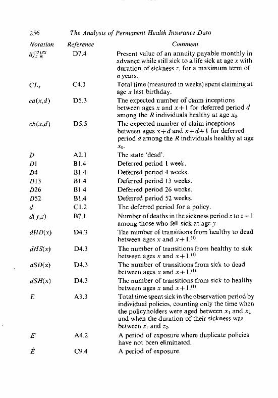
256
Notation .,(12)SS
~ X . Z
CL,
ca(x,d)
ch (x,d)
D D I D4 D13 D26 D52 d d(?,4
dHD(x)
dHS(x)
dSD(x)
dSH(x)
E
- ~~ ~
The Anabsis of Permanenf Heallh Insurance Data
Reference D7.4
C4.1
D5.3
D5.5
A2.1 81.4 B1.4 81.4 81.4 B1.4 C1.2 87.1
D4.3
D4.3
D4.3
D4.3
A3.3
Commenl Present value of an annuity payable monthly in advance while still sick to a life sick at age x with duration of sickness 2, for a maximum term of n years. Total time (measured in weeks) spent claiming at age x last birthday. The expected number of claim inceptions between ages x and X + l for deferred period d among the R individuals healthy at age xo. The expected number of claim inceptions between ages X + d and x + d+ l for deferred period damong the R individuals healthy at age Jo.
The state 'dead'. Deferred period 1 week. Deferred period 4 weeks. Deferred period 13 weeks. Deferred period 26 weeks. Deferred period 52 weeks. The deferred period for a policy. Number of deaths in the sickness period z to z+ 1 among those who fell sick at age y. The number of transitions from healthy to dead between ages x and X + I ."I
The number of transitions from healthy to sick between ages x and X + 1.'') The number of transitions from sick to dead between ages x and X + l . ( l )
The number of transitions from sick to healthy between ages X and X + l.(') Total time spent sick in the observation period by individual policies, counting only the time when the policyholders were aged between X, and xz and when the duration of their sickness was between zl and 2 2 .
A period of exposure where duplicate policies have not been eliminated. A period of exposure.

Reference C1.2
83.2
C4.1
C3.3
Appendix A
C2.1
A4.2
83.2
C4.4
B3.2
A2.1 D2.1 A4.4
A4.5
C1.2
C9.4 C7.2
C3.2 C3.2 C7.2
Clossarj, of Notation 257
Comment Total time spent in the observation period by individuals who are healthy and aged between XI
and .q. The exposed to risk for the data cell for mean age y and mean sickness duration z.
Time spent in 1975-78 as healthy by policyholders aged X last birthday. The period of exposure in the ith week following the end of the deferred period. A period of exposure for individuals having exactly t policies. Factors used to calculate Manchester-Unity- type exposures exactly. The proportion of policyholders having exactly t policies. Function of age v at sickness inception, being a factor of recovery intensity p,+; , , . Annual rate of growth of the number of policies in force. Function of sickness duration z, being a factor of recovery intensity p,+,l. The state 'healthy'. The step size for the numerical algorithms. The number of sicknesses among policies with deferred period d which start in the observation period and for which the policyholder is aged between X, and X? at the start of the sickness and which last beyond the deferred period. A number of claim inceptions, where duplicate policies have not been eliminated. Number of sicknesses which start in the observation period, with age at start of sickness between X, and X*, and which last beyond the deferred period of the policy. Expected number of claim inceptions. Expected number of sicknesses lasting 4 weeks beyond the end of the deferred period. The number of claim inceptions not reported. The number of claim inceptions reported. The number of claims lasting 4 weeks beyond the end of the deferred period.

-
The Analysis of Permanent Health Insurance Data
Reference D7.2
DS.4
D5.4
E8.4
E8.4
D5.5
C9.9
D5.2
E8.5
E8.5
87.1
D4.2 D4.2
D4.2 D4.2 D4.2 D4.2 D4.2 A4.4
D2.2
Comment The rate of interest for calculating monetary functions. The claim incevtion rate of tvve (a) at ace X for -. ~ , - deferred period d.'" The claim inception rate of type (a) at age X for deferred period dfor a life who was healthy at age X- t.(') The ultimate claim inception rate of type (a) at age X for deferred period d. The select claim inception rate of type (a) at attained age X for deferred period d, for a life who was healthy at age X- t. The claim inception rate of type (b) at age X for deferred period d.") A function linking claim termination rates for D l and 026 . The expected number of years lived between ages X and X+ l by the R individuals who were healthy at age xo?) The value of L, conditional on being healthy at age xo. The select value of L,,, , for a life who was healthy at age .q,.
Number of claims remaining in force at exact sickness duration r for lives aged exactly y at the date of falling sick. The number dead at age X.(')
The number dead at age x having died as healthy.") The number dead at age X, having died as sick.") The number healthy at age X.(') The number alive at age X.(') The number sick at age X.(') The number alive at age X; the same as lL(x).") The number of policyholders at time t who are healthy, aged betweenxl and XI and have policies with deferred period d.
The transition intensity from healthy to dead at age X; the same as p,.
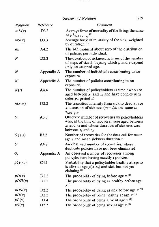
Glossary of Notation 259
Reference
D3.3
D3.3
A4.2
D2.3
Appendix A
Appendix A
A4.4
D2.2
A3.3
83.2
A4.2
Appendix A
C4.1
D2.2 D2.2
D2.2 D2.2 D3.4 D2.2
Comment
Average force of mortality of the living; the same as ( I 1
Average force of mortality of the sick, weighted by duration.(l' The i-th moment about zero of the distribution of policies per individual. The duration of sickness, in terms of the number of steps of size h, beyong which p and v depend only on attained age. The number of individuals contributing to an exposure. The number of policies contributing to an exposure. The number of policyholders at time 1 who are aged between x l and x2 and have policies with deferred period d. The transition intensity from sick to dead at age X, duration of sickness (m-$)h; the same as v., cm -$h.
Observed number of recoveries by policyholders who, at the time of recovery, were aged between XL and X> and whose duration of sickness was between zl and z2.
Number of recoveries for the data cell for mean age y and mean sickness duration z.
An observed number of recoveries, where duplicate policies have not been eliminated. An observed number of recoveries among policyholders having exactly t policies. Probability that a policyholder healthy a t age xa is alive at age y(>xo) and sick but not yet claiming.'l] The probability of dying before age X."' The probability of dying as healthy before age x.(I' The probability of dying as sick before age X.("
The probability of being healthy at age X.'"
The probability of being alive at age X.(') The probability of being sick at age X.(')

The Analysis of Permanent Health Insurance Data
Reference Comment The probability of being sick at age X, with duration of sickness between ( m - l ) h and mh.(') The probability of being sick at age X, with duration of sickness greater than Nh."' The probability of being sick at age X , with duration of sickness between a and a + b.") An average value of X,..., over the year of age X to x + l . The proportion of TE, spent as sick but not yet claiming. The probability of remaining healthy from age .X
to age X + t . The same as ,px5 The probability of remaining sick from age x to age x + t given duration of sickness z at age X.
The probability of being in state k at age x + t , conditional on being in state j at age x with duration z .
Probability of surviving for r years of a select life entering at age X .
The probability of being sick at age x + t with duration not more than W , conditional on being healthy at age X .
The proportion of policyholders at time t who are sick and claiming. The proportion of policyholders at time t who are sick but not yet claiming. The value of q , for attained age X for a life who was healthy at age X - t . The probability of death within I year for those living at age A'); or (E7.3) the ultimate mortality rate at age X.
The select mortality rate at age x for a life who was healthy at age X - t . Independent rate of death in the short interval h. Independent rate of recovery in the short interval h. Probability of death within t years of a life who was healthy at age X.
The radix for the incrementaecrement table.

Notation Reference
Glossary of Notation 261
Comment
The number of reported recoveries in the i-th week following the end of the deferred period. The transition intensity from sick to healthy at age X, duration of sickness (m-+)h; the same as P ~ . ( ~ - j ' h .
Number of recoveries in the sickness period z to i+ l among those who fell sick at age g. The state 'sick'. The transition intensity from healthy to sick at age X; the same as o,.
The number of years selection in a select table of mortality rates, inception rates or sickness rates. The start of an observation period. The end of an observation period. Total time spent in the observation period 1975- 78 at age X last birthday. Total number of claim inceptions for deferred period d, for a life healthy at age xo, within n years. Equivalent version of Tca(xn,d,n) using select tables. The factor by which the variance of the estimator for U is inflated by the presence of duplicate policies in the data. The usual discounting factor (l + I)-'. The number of 'non-reported recoveries' in the i-th week following the end of the deferred period. The attained age of a policyholder. An age at which the policyholder is healthy. The state of the individual (healthy, sick or dead) at age X.
Age at start of sickness. Duration of the sojourn so far in the current state, Y(x). The duration so far of the policyholder's current sickness. The central rate of sickness at age X, with duration of sickness between a and a + b."'

The Analysis of Permanent Health Insurance Data
Reference E9.1
A1.2
E9.2
C2.1
C2.1
D6.1
A2. 1
D3.2
A2.1
C9.9 C9.9 A4.4
C7.2
C1.2
C9.9
A3.3
Commen 1
The value of z(x,a/b) for a life aged X who was healthy a t age X- t.
A (Manchester-Unity-type) rate of sickness or (E9.2) the ultimate rate of sickness for attained age X , sickness period alb. The select rate of sickness for attained age X,
sickness period alb, for a life who was healthy at age X - t . Sum over each of the 4 years of the number of policies at the start of the year for which the policyholders were either aged x nearest birthday and entered in the previous calendar year or were aged X + 1 nearest birthday and entered between 1 and 2 years ago. Sum over each of the 4 years of the number of policies a t the start of each year for which the policyholders were aged X+ l nearest birthday and who entered in the previous year. 52 times the probability that an individual is sick at age X with duration of sickness between a and a+b.cl) The transition intensity from healthy to dead at age X. The transition intensity from living to dead at age x,+t.( l) The transition intensity from sick to dead at current age x and current duration of sickness z. The value of v , , for a D 1 policyholder. The value of v , , for a D26 policyholder. - The assumed constant value of ,p,SS over the interval [x,,x,l.
The probability that a sickness lasts for at least 4 weeks beyond the deferred period. The probability that an individual who falls sick at age x willremain sick for at least period d; the same as .pp. The value of n, with d=26 weeks for a D 26 policyholder. The assumed constant value of p, , over the rectangle [x,,xzl x [z~,z~].

Notation
P'
Psr
Reference A4.2
Glossary of Notation 263
Comment The maximum likelihood estimate of p where duplicate policies have not been eliminated. The maximum likelihood estimate of p where b=O/E . An estimate of p in the i-th week following the end of the deferred period. An estimate of p in the i-th week following the end of the deferred period allowing for 'non- reported recoveries'. The transition intensity from sick to healthy at current age x and current duration of sickness z .
The value of p,, for a D I policyholder. The value of p , , for a D26 policyholder. The assumed constant value of ux over the interval [xl,xz]. The transition intensity from healthy to sick at age X. An estimator for U where duplicates have not been eliminated. The maximum likelihood estimator for U.
The value of ux for a D 1 policyholder. The value of ux for a D26 policyholder.

. . . . . . . . . . . . . . . . . . . . . . . . . . Intr oducti011...
.......... The Analyek of Pamrtnent Health Insurance Data , ~ . Intmduction . . . . . . . . . . . . . . . . . . . . . . . . . . . . . . . . .
Part A: .A Multiple State Modcl Permanent Heal* Insurana by H, R. Waters ... ... . . . . . . . . . . . . . . . . . . . . .
Fart B: ThcGraduationof C l a i m R e c o v e r y M b M o ~ h ~ ? & % by P. H. Bayliss . . . . . . . . . . . . . . . . . . . . .
Part C: The ~raduatioi of Sickness Inception inttmsitb by H, R. Waters . . . . . . . . . . . . . . . . . . . . . . . . . . .
2 Part D: Computational Procedure for the Model U
. . . . . . . . . . . . . . . . . . . . . . . . . . . . by H. R. Waters ... Part E: Calculation of Robabditi m... . . . . . . . . . . . . ..:.
Part F: h a t i o n of ~onetary h unctions ............... . . . . . . . . . . . . . . . . . . . . . . . . . . . . . . . . . . . . Referernoes
Oloasary of Notation . . . . . . . . . . . .