context free languages and push down automataassets.press.princeton.edu/releases/m11348.pdf ·...

Appendix A

Context free languagesand push down automata

This document is an appendix to the book What Can Be Computed?:A Practical Guide to the Theory of Computation by John MacCormick(Princeton University Press, 2018).

Previously, we have seen two distinct computational models: Turingmachines (chapter 5), and finite automata (chapter 9). These two modelsrepresent two extremes in the world of computability. On the one hand,Turing machines are as powerful as any physically-realistic computer. Onthe other hand, the finite automaton seems to be the weakest computationalmodel that deserves serious study: it can decide regular languages butnothing else, making it strictly weaker than the Turing machine. Are thereany interesting models between these two extremes? The answer is “yes, butnot many.” Surprisingly, there are only a few useful models of intermediatepower. Of these, the most important are the push down automata (pdas),which are the main topic of this chapter.

To understand pdas, we must first understand one of the most funda-mental data structures in computer science: the stack. As you probablyknow, a stack is a data structure that allows you to store as many pieces ofinformation as you want, but the only way to access the information is tolook at, and optionally remove, the top of the stack. It might help to thinkof having a large supply of blank cards in a desk drawer and a desktopwhere you can store a single pile (i.e. stack) of cards that have symbolswritten on them. There are two operations you can perform on this pile:

Push You can take a blank card from the drawer, write a symbol s on the

1

© Copyright, Princeton University Press. No part of this book may be distributed, posted, or reproduced in any form by digital or mechanical means without prior written permission of the publisher.

For general queries, contact [email protected]

2 Appendix A. What Can Be Computed?

card, and place it on top of the pile. We say you have pushed thesymbol s onto the stack.

Pop Provided the stack isn’t empty, you can pick up the top card from thepile, look at the symbol s, then throw the card in the trash. We sayyou have popped the stack, obtaining the symbol s.

Recall that a finite automaton is a specialized, restricted form of Turingmachine: it can’t edit the tape, and its read-write head always moves to theright. A pda is also a restricted form of Turing machine, although it’s notusually described like that. Usually, a pda is described as a finite automatonaugmented with a stack. Perhaps a sensible name for these things wouldbe “stack automata.” Why are they instead called “push down automata”?This comes from a commonly-used physical analogy for stacks. Sometimeswe think of a stack as being spring-loaded, so that every time we add a newitem to the top, everything gets “pushed down” and the top of the stackstays at the same level. Some cafeterias use a system like this with stacksof dining plates.

Pdas come in two flavors: we have the deterministic pda (dpda) and thenondeterministic pda (npda). Surprisingly, and very importantly, dpdasand npdas are not equivalent in terms of computational power. This willbe one of the main results of the chapter, demonstrating that (in contrastwith dfas/nfas, and dtms/ntms) nondeterminism can affect computability.We won’t give a proof of the non-equivalence of dpdas and npdas, but wewill see a persuasive example at the end of section A.1.

The other key result of the chapter is that pdas correspond to a funda-mental and important class of languages known as context free languages(cfls). Cfls are a central concept in the theory of compilers and program-ming languages. It turns out that an understanding of pdas is very usefulfor building practical compilers. The proof of equivalence for pdas and cflsis given in sections A.3 and A.5.

A.1 Definition and examples of pdas

We mentioned above that a pda can be thought of as a finite automatonaugmented with a stack. Our formal definition, however, is based on Turingmachines:

Pda, dpda, and npda. A pda is a 2-tape Turing machine withthe additional properties (1)–(4) below. If the Turing machineis deterministic, we have a deterministic pda or dpda. If theTuring machine is nondeterministic, we can emphasize this by



Appendix A. What Can Be Computed? 3

calling it an npda, but the term “pda” incorporates both npdasand dpdas. The two tapes of a pda have special names: the firsttape is called the input, and the second tape is called the stack.The input has the same restrictions as a finite automaton withε-transitions:

(1) Cells on the input tape cannot be altered.

(2) The head for the input tape always stays or moves to theright (it cannot move left).

The stack tape is restricted to push and pop operations, formal-ized as follows:

(3) The stack is initially empty (i.e. the stack tape containsonly blank symbols).

(4) The only permitted sequences of operations on the stacktape are:

� (Push) Write a non-blank symbol s, then move rightone cell.

� (Pop) Move left one cell, read symbol s, then overwrites with a blank and stay at the current cell.1

Naturally, the input to a pda is provided at the start of the input tape beforethe computation begins. By definition, this input consists of a sequence ofnon-blank symbols followed by infinitely many blanks.

The easiest way to describe a specific pda is via a transition diagram,such as figure A.1. The details of this figure will be explained shortly.First, let’s understand the specialized notation on these transition dia-grams, which is somewhat different to the finite automaton and Turingmachine notation from earlier chapters. Specifically, each transition is la-beled

X, s; s1

where X is the scanned input tape symbol, s is the popped stack symbol,and s1 is the symbol (or symbols, as described soon) pushed back onto thestack. For example, the transition label

C,g;a means “if the scanned input symbol is C and thepopped stack symbol is a g, push an a ontothe stack and move right to the next inputsymbol.”

1Attempting to pop an empty stack is equivalent to doing nothing. In terms of theunderlying Turing machine operations, this corresponds to our convention that com-manding a Turing machine to move left from cell 0 leaves the head where it is.




Figure A.1: A pda solving the problem ContainsNANA.

Any or all of the three components can be replaced with ε, as the followingexamples show:

ε,g;a means “if popped g, then push a, and don’t moveinput head”

C, ε;a means “if scanned C, then push a without poppinganything, and move input head right”

C,g; ε means “if scanned C and popped g, move input headright”

C, ε; ε means “if scanned C, move input head right withoutaltering the stack”

Figure A.1 provides a concrete example. This pda solves the problemContainsNANA, which searches a string for one of the substrings “CACA”,“GAGA”, “TATA”, or “AAAA” (for details, see figure 8.1). As with the tran-sition diagrams in earlier chapters (see section 5.1), we allow abbreviatednotation, so “! ” matches any single symbol other than a blank.

Hence, our containsNANA pda is nondeterministic. When reading aC, G, A, or T, the state q0 produces two clones: one returns to q0, and theother advances to q1. Note how the stack is used to remember the firstcharacter of the string to be matched. For example, whenever the pdaencounters a G, one of the clones pushes “g” onto the stack and transitionsto q1. If the next input symbol is an A, the pda moves to q2. At this point,the clone rejects unless the top stack symbol matches the scanned inputsymbol. In our specific example, then, the pda transitions to q3 only if thenext input symbol is a G.

The containsNANA pda illustrates a useful convention: it often im-proves readability to use a separate input alphabet and stack alphabet. Inthis book, we will typically use uppercase letters for the input and lower-case letters for the stack. This is not formally required by the definitionof a pda, but it does make it easier to read transitions like “C,g; ε.” The




Figure A.2: Top: The pda GnTn, which decides the language GnTn. Bot-tom: The pda GnT2n, which decides the language GnT2n. The only differ-ence between these pdas is in the q1 Ñ q1 transition.

alphabet for the underlying Turing machine is just the union of the inputand stack alphabets.

The book materials provide the simulators simulateDpda.py andsimulateNpda.py for deterministic and nondeterministic pdas respec-tively. The format for describing pdas in ASCII is similar to the Turingmachine descriptions in chapter 5 and the finite automata descriptions inchapter 9. ASCII descriptions of all pdas in this chapter are providedwith the book materials; see containsGAGA.pda containsNANA.pdafor specific examples. The simulators can be invoked using the same styleof commands as for Turing machines and finite automata:

>>> simulateDpda(rf('containsGAGA.pda'), 'TTGAGATT')>>> simulateNpda(rf('containsNANA.pda'), 'TTGAGATT')

Note that our containsNANA pda decides a language that can also bedecided by an nfa (or dfa). The nfa would need more states: instead ofa single q1, for example, we would need four separate states to rememberwhich character needs to be matched. So in this case, the presence of thestack yields a more compact automaton but doesn’t appear to provide extracomputational power.




In contrast, our next two pda examples demonstrate that pdas arestrictly more powerful than dfas and nfas. The top panel of figure A.2shows a pda called GnTn that decides the language GnTn. In section 9.5,we proved that this language cannot be decided by any dfa or nfa. Hence,this example provides an immediate proof that pdas are more powerful thandfas.

Let’s investigate the GnTn pda in more detail. Its first action, in theq0 Ñ q1 transition, is to push the symbol “z” onto the stack withoutreading any input. This is a trick that our pdas will use frequently: there isno built-in way of recognizing the bottom of the stack, but we can achievethis by pushing a unique symbol onto the stack before doing anything else.In this book, we will always use “z” to mark the bottom of the stack, butof course any other symbol could be used for that purpose.

After this, the GnTn pda loops in q1, pushing one “g” for every “G”encountered in the input. As soon as a “T” is encountered, it pops a “g”and switches to q2, where it continues to pop one “g” for every “T”. Theautomaton accepts if and only if the blank marking the end of the input isencountered at the same time that the bottom of the stack (“z”) is popped.This means the number of g’s pushed equals number of g’s popped, so thenumber of G’s equals the number of T’s. The lower curved transition enablesthe special case of the empty string being accepted. Thus, the pda acceptsprecisely the strings of the form GnTn for n ¥ 0.

The lower panel of figure A.2 shows a slight variant. The only differenceis the q1 Ñ q1 transition, which pushes two g’s instead of one. The notationfor this transition, “G, ε;gg”, demonstrates another useful convention forour transition diagrams: we allow a single transition to push two or moresymbols onto the stack, if desired. This is just a notational convenience,since we could have written out a sequence of states that push one symbolat a time instead. The order of the pushes runs right to left. For example:

C,g;abc means “if the scanned input symbol is C and thepopped stack symbol is a g, push a c, thena b, then an a onto the stack, and move rightto the next input symbol.”

Returning to the lower panel of figure A.2, let’s determine what languageit decides. The input must begin with some G’s, say n of them. For eachof these G’s, two g’s get pushed. So, immediately before the first T isencountered, there are 2n g-symbols on the stack. For the remainder of theinput, one g is popped for every T. Thus, the PDA accepts precisely stringsof the form GnT2n for n ¥ 0. Although we didn’t explicitly prove it inchapter 9, it’s easy to see that this language is also irregular and therefore




another example of the extra power of pdas. The next claim summarizesthese observations.

Claim A.1 There exist non-regular languages that can be decided bydpas. Hence, dpdas are strictly more powerful than dfas or nfas.

Proof of the claim. To prove the claim, we need only a single exampleof a non-regular language that is decidable by a dpda. The GnTn examplediscussed above is a suitable example. l

The GnTn example shows us how we can use a pda’s stack to countthings. In the next example, we use it for a more detailed comparison.For this, we need some new notation. Given a string s, write sR for thereverse of s. For example, if s � “GAT” then sR � “TAG”. (We used asimilar notation to reverse an entire language in section 9.7; now we useit to reverse individual strings.) Recall that a palindrome is a string thatreads the same backwards as forwards. More formally, s is a palindromeif s � sR. For example, the following are all palindromes: ε, “G”, “GG”,“CTC”, and “GTTATTG”. We use this idea to define two new languages thatform palindromes from “A” and “T” characters:

EvenPalindromes � ts � pT |Aq� such that s � sR and |s| is evenu

MarkedPalindromes � ts � pT |Aq� C pT |Aq� such that s � sRu

So EvenPalindromes contains strings such as “ATTA” and “TTAATT”,whereas MarkedPalindromes contains strings such as “ACA” and “TTACATT”.The key difference is that, in MarkedPalindromes, the center of eachstring is marked with a “C”. In EvenPalindromes, we can only deter-mine the center of the string by examining the entire string. By the way,we consider palindromes of even length purely to simplify the pda thatdecides this language. It is a useful exercise to create a pda that decidespalindromes of any length.

Figure A.3 shows pdas deciding each of our palindrome languages. Thesepdas use the same trick of pushing a “z” to mark the bottom of the stack.The key observation is that state q2 pops “A” and “T” characters in pre-cisely the reverse order that they were pushed on in state q1—by definition,stacks release their contents in the reverse of the insertion order. This ishow we enforce the requirement that the string reads the same backwardsor forwards.

The only difference between the two pdas of figure A.3 is in the tran-sition from q1 to q2. The top pda can follow this transition at any timewithout consuming any input or stack symbol, whereas the bottom pdainsists on reading the center-marking “C” before transitioning to q2. Thisapparently-small difference is deceptive: it means that the top panel’s q1 is




Figure A.3: Top: An npda deciding the language EvenPalindromes.Bottom: A dpda deciding the language MarkedPalindromes. The onlydifference between these pdas is in the q1 Ñ q2 transition.

nondeterministic, since any “A” or “T” in the input string offers the choiceof remaining in q1 or transitioning to q2. In effect, the top pda launches anew clone for every “A” or “T”, just in case the scanned input symbol is thestart of the second half (that is, the reversed half) of the string. The bot-tom pda doesn’t need this nondeterminism: because of the center-marking“C”, it can tell exactly when it reaches the middle of the string. In fact, acareful analysis of each transition in the bottom pda reveals that the entirepda is deterministic.

It turns out that we have encountered a truly fundamental differencebetween EvenPalindromes and MarkedPalindromes: we constructedan npda that decides EvenPalindromes, but it can be shown that nodeterministic pda decides EvenPalindromes. This important and sur-prising difference between npdas and dpdas is highlighted in the followingclaim.

Claim A.2 There exist languages that can be decided by an npda butnot by any dpda.

The proof of this claim lies beyond the scope of this book and is omitted,but the example of figure A.3 is persuasive. Spend a few minutes trying toconstruct a dpda for EvenPalindromes! The set of languages that canbe decided by dpdas is known as the deterministic context free languages.




We briefly return to this concept in section A.6.We finish our overview of the computational power of pdas by stating

another result without proof, this time demonstrating that Turing machineshave strictly greater power than pdas.

Claim A.3 There exist languages that can be decided by a Turing ma-chine but not by any pda.

Again, a proof of this claim is beyond the scope of this book, but wecan provide a few hints about why it is true. One example of a languagethat can’t be decided by pdas is tGnTnAn |n ¥ 0}, or GnTnAn for short.Clearly, GnTnAn can be decided by a Python program and hence by aTuring machine. But it can be shown that, because they have only a singlestack, pdas can’t keep track of both matching pairs of G’s and T’s andmatching pairs of T’s and A’s. The proof employs a more advanced variantof the pumping lemma, known as the “pumping lemma for context freelanguages.”

A.2 Context free grammars

In computer science, a “grammar” is a set of rules for producing strings.Let’s start with an informal example:

sÑ CGaT

aÑ ε |Aa

Our grammars will always generate strings by begining with the start sym-bol, usually denoted s. Symbols appearing on the left-hand side of a rule(before the “Ñ”) are called variables. In this book, variables will usuallybe lowercase ASCII letters; the variables in the example above are s and a.The remaining symbols are called terminals. In this book, terminals willusually be uppercase ASCII letters; the terminals in the example above areC, A, G, and T. In most of our examples, we will restrict the terminals tothis genetic alphabet. In general, of course, the variables and terminalscould be drawn from any disjoint alphabets.

The rules in the example grammar above tell us we can replace “s”with “CGaT”, and we can replace “a” with either ε or “Aa”. Rules can beapplied as many times as we wish. For example, in this grammar we canobtain the sequence

sÑ CGaTÑ CGAaTÑ CGAAaTÑ CGAAT.




A sequence like this is called a derivation. Any string that can be derivedis called a sentential form. In our example, sentential forms include “s”,“CGaT”, “CGAAaT”, and “CGAAT”. Most often, we are interested in de-riving strings that contain no variables. We call these terminal strings, orjust strings. So, “CGAAT” is a terminal string generated by our examplegrammar, whereas “CGAAaT” is a sentential form but not a terminal string.The set of all terminal strings that can be derived by a grammar G is calledthe language generated by G. It’s easy to see that the language generatedby our example grammar is represented by the regular expression CGA�T.

Grammars are an important and fundamental concept. They can beused to unify all of theoretical computer science. For example, there existsa class of regular grammars that generate all regular languages. Everyregular grammar G corresponds to some dfa D (and vice versa), such thatD decides the language generated by G. Similarly, there exists a classof unrestricted grammars that generate all recognizable languages. Everyunrestricted grammar G corresponds to some Turing machine M (and viceversa), such that M recognizes the language generated by G. This fact isparticularly important for historical reasons, since researchers such as EmilPost developed a complete theory of computation based on unrestrictedgrammars, independently of Alan Turing’s development of the theory interms of Turing machines.

Despite their fundamental importance, we mostly ignore grammars inthis book. Our approach is instead based on Turing machines and specialcases of Turing machines, such as dfas and pdas. However, there is oneclass of grammars that we cannot ignore, since it is ubiquitous in com-puter science. This is the class of context free grammars. Here’s a formaldefinition:

Context free grammar, context free language. A con-text free grammar (cfg) consists of: an alphabet of variablesincluding the start symbol, a separate and disjoint alphabet ofterminals, and a finite set of rules. Each rule maps a singlevariable to a string of variables and terminals.

A language generated by a cfg is called a context free lan-guage (cfl).

As a notational convenience, we often combine rules that map a givenvariable using the vertical bar, “|”. For example, our initial example at thestart of section A.2 combined the two rules a Ñ ε and a Ñ Aa into themore compact notation aÑ ε |Aa.

What makes a grammar “context free”? The key part of the definitionis that the left-hand side of any rule contains exactly one variable. Moregeneral grammars allow additional constraints on the left-hand side, as in




the rule aGÑ ATG, which allows us to replace the variable “a” with “AT”only when the “a” is followed by a “G”. In other words, this rule can onlybe applied when the “context” of the variable includes a “G” on the right.By insisting that the left-hand side of a rule contains only a single variablev, we are declaring that the rule can be applied whenever v occurs in asentential form, regardless of v’s context.

Derivation trees and ambiguity

Let’s now focus our attention on the following cfg, which we’ll call G1:

sÑ sc |st | ε

cÑ CAT (A.1)

tÑ TAG

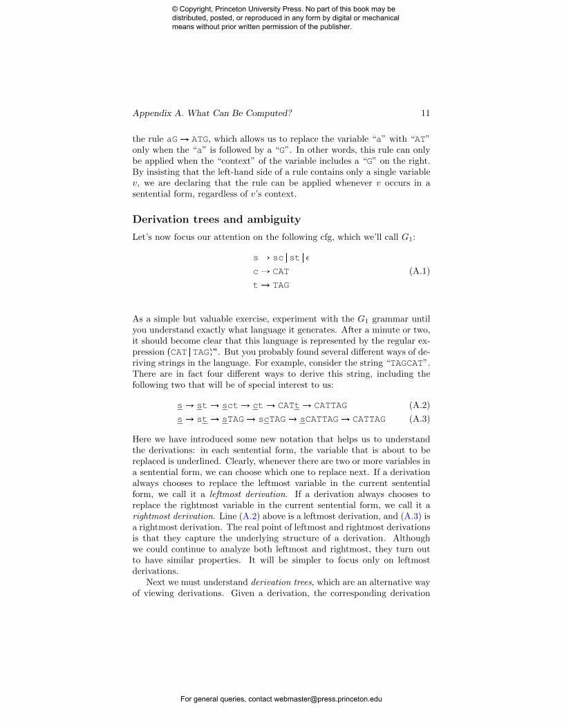
As a simple but valuable exercise, experiment with the G1 grammar untilyou understand exactly what language it generates. After a minute or two,it should become clear that this language is represented by the regular ex-pression pCAT |TAGq�. But you probably found several different ways of de-riving strings in the language. For example, consider the string “TAGCAT”.There are in fact four different ways to derive this string, including thefollowing two that will be of special interest to us:

sÑ stÑ sctÑ ctÑ CATtÑ CATTAG (A.2)

sÑ stÑ sTAGÑ scTAGÑ sCATTAGÑ CATTAG (A.3)

Here we have introduced some new notation that helps us to understandthe derivations: in each sentential form, the variable that is about to bereplaced is underlined. Clearly, whenever there are two or more variables ina sentential form, we can choose which one to replace next. If a derivationalways chooses to replace the leftmost variable in the current sententialform, we call it a leftmost derivation. If a derivation always chooses toreplace the rightmost variable in the current sentential form, we call it arightmost derivation. Line (A.2) above is a leftmost derivation, and (A.3) isa rightmost derivation. The real point of leftmost and rightmost derivationsis that they capture the underlying structure of a derivation. Althoughwe could continue to analyze both leftmost and rightmost, they turn outto have similar properties. It will be simpler to focus only on leftmostderivations.

Next we must understand derivation trees, which are an alternative wayof viewing derivations. Given a derivation, the corresponding derivation




Figure A.4: Derivation tree for “CATTAG” in the G1 grammar.

tree is defined recursively: the root node is the start symbol s, and thechildren of any node v are the symbols produced when a rule is appliedto v. The children must of course be listed in order from left to right, asspecified by the rule that produced them. The yield of a derivation treeis the string formed by concatenating the leaves of the tree from left toright. Figure A.4 gives a derivation tree of “CATTAG” in the G1 grammar;note that the yield is indeed “CATTAG”. Before reading on, trace out theleftmost and rightmost derivations on this tree, and convince yourself ofthe simple correspondence between the tree and these derivations.

It follows immediately from the definition of derivation tree that theinternal nodes are all variables and the leaf nodes are all terminals or ε.It’s also easy to see that a given derivation tree corresponds to a uniqueleftmost derivation, obtained by generating the tree in the standard left-first, depth-first order. Thus, there is a one-to-one correspondence betweenderivation trees and leftmost derivations.

Is it possible for a string to have two different leftmost derivations? (Orequivalently, can a string have two different derivation trees?) Unfortu-nately, the answer is yes. Consider the following cfg, denoted G2, whichadds two new rules to G1:

sÑ sc |st | ε

cÑ CAT |CA

tÑ TAG |AG

Now consider the string “CATAG”. As a simple but important exercise,try to write down two distinct leftmost derivations and two distinct deriva-tion trees for this string, before looking at the solutions below. Hopefully,




Figure A.5: Distinct derivation trees for “CATAG” in the G2 grammar..

you were able to obtain the following leftmost derivations, where the onlydifference is in the fifth sentential form:

sÑ stÑ sctÑ ctÑ CATtÑ CATAG (A.4)

sÑ stÑ sctÑ ctÑ CAtÑ CATAG (A.5)

The difference is more obvious in the trees of figure A.5, where wesee immediately that the terminal “T” has a different parent in the twoderivations. This situation is called ambiguity. Formally, a terminal stringis ambiguous if it has two distinct leftmost derivations (or equivalently,two distinct derivation trees). A cfg is ambiguous if it has one or moreambiguous terminal strings in its language.

So, we have already proved that G2 is an ambiguous cfg, since we exhib-ited a string with two distinct leftmost derivations. Interestingly, however,the problem of ambiguity in G2 can be fixed. We will now describe a newcfg, G3, which generates the same language as G2, yet is not ambiguous.The rules of G3 are:

sÑ sc |sa |scT |sTa | ε

cÑ CA

tÑ AG

We leave it as an exercise to prove that G3 is in fact unambiguous andgenerates the same language as G2.

Ambiguity in context free grammars is a subtle and fascinating topic,but we don’t dwell on it here. Instead, we will state without proof twoimportant facts about ambiguity:

� There do exist inherently ambiguous cfgs: that is, cfgs that cannotbe reformulated to remove ambiguity, as we can do with G3 above.




sÑ sc |st | ε

cÑ CAT

tÑ TAG

Figure A.6: Left: The grammar G1, which generates the language L repre-sented by the regex pCAT |TAGq� (see section A.2). Right: A pda equivalentto G1. This pda recognizes the language L and is provided with the bookmaterials as cattag.pda. For additional explanatory details, experimentwith showCATTAGhist.py.

Consequently, there exist ambiguous context-free languages, which aregenerated only by ambiguous cfgs. One example of an ambiguous cflis

tCnAmTk such that n � m or m � ku.

� Let AmbiguousCfg be the decision problem that asks whether agiven cfg is ambiguous. Then AmbiguousCfg is undecidable.

A.3 Converting a cfg to a pda

We now turn to the most important result of this chapter, which is thatpdas recognize precisely the set of context free languages. Note carefullythe use of the word “recognize” rather than “decide” here, and if necessaryreview section 4.5 to understand the difference between these concepts. Forthe remainder of this chapter, we focus only on recognizing languages andnot deciding them. The reason is that there is no easy way for grammarsto reject a string. Grammars generate strings. So we can imagine using a




stepnumber

state tapestack(top to the left)

0 q0: C A T ε

1 q1: C A T sz

2 q1: C A T scz

3 q1: C A T cz

4 q1: C A T CATz

5 q1: C A T ATz

6 q1: C A T Tz

7 q1: C A T z

8 qaccept: C A T ε

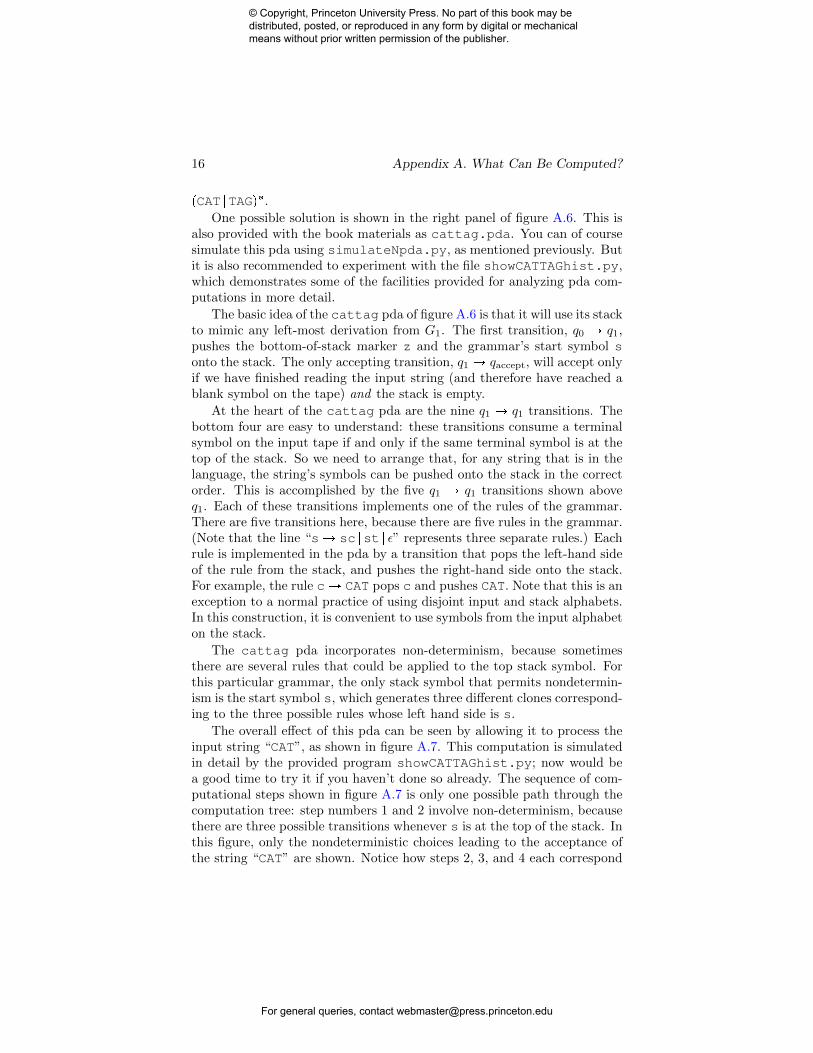
Figure A.7: A complete computation of the pda in figure A.6, acceptingthe string “CAT”. Note that the computation tree of this pda for the input“CAT” is infinite. The computation shown here is the only path leadingto a positive leaf in the computation tree. It corresponds to the leftmostderivation sÑ scÑ cÑ CAT.

grammar to create a list of all the strings in a language: begin with thestart symbol, and repeatedly apply all of the possible rules in the grammar.This approach will never terminate, but it will generate every string in thelanguage of the grammar. Thus, given any particular string S, we willeventually recognize S if it is in the language. But there is no obvious wayof rejecting S if it is not in the language.2

Therefore, we aim to prove that cfgs and pdas are equivalent in the sensethat they recognize the same class of languages. To prove this result, wewill need to show that (i) given any cfg G, there exists a pda that recognizesthe language generated by G; and (ii) Given any pda M , there exists a cfgthat generates the language recognized by M . In this section, we provepart (i).

Before giving a general proof of (i), it will be helpful to examine adetailed example. Figure A.6 presents this example, which is based on thegrammar G1. The rules of G1 are shown again in the left panel of figure A.6.Recall that G1 was first introduced in section A.2, where we saw that itgenerates the language L represented by the regex pCAT |TAGq�. So ourchallenge is to come up with a pda that recognizes any string of the form

2The question of membership in a context free language is decidable: a cubic-timealgorithm known as CYK achieves this. But CYK itself runs on a Turing machine, nota pda.




pCAT |TAGq�.

One possible solution is shown in the right panel of figure A.6. This isalso provided with the book materials as cattag.pda. You can of coursesimulate this pda using simulateNpda.py, as mentioned previously. Butit is also recommended to experiment with the file showCATTAGhist.py,which demonstrates some of the facilities provided for analyzing pda com-putations in more detail.

The basic idea of the cattag pda of figure A.6 is that it will use its stackto mimic any left-most derivation from G1. The first transition, q0 Ñ q1,pushes the bottom-of-stack marker z and the grammar’s start symbol sonto the stack. The only accepting transition, q1 Ñ qaccept, will accept onlyif we have finished reading the input string (and therefore have reached ablank symbol on the tape) and the stack is empty.

At the heart of the cattag pda are the nine q1 Ñ q1 transitions. Thebottom four are easy to understand: these transitions consume a terminalsymbol on the input tape if and only if the same terminal symbol is at thetop of the stack. So we need to arrange that, for any string that is in thelanguage, the string’s symbols can be pushed onto the stack in the correctorder. This is accomplished by the five q1 Ñ q1 transitions shown aboveq1. Each of these transitions implements one of the rules of the grammar.There are five transitions here, because there are five rules in the grammar.(Note that the line “sÑ sc |st | ε” represents three separate rules.) Eachrule is implemented in the pda by a transition that pops the left-hand sideof the rule from the stack, and pushes the right-hand side onto the stack.For example, the rule cÑ CAT pops c and pushes CAT. Note that this is anexception to a normal practice of using disjoint input and stack alphabets.In this construction, it is convenient to use symbols from the input alphabeton the stack.

The cattag pda incorporates non-determinism, because sometimesthere are several rules that could be applied to the top stack symbol. Forthis particular grammar, the only stack symbol that permits nondetermin-ism is the start symbol s, which generates three different clones correspond-ing to the three possible rules whose left hand side is s.

The overall effect of this pda can be seen by allowing it to process theinput string “CAT”, as shown in figure A.7. This computation is simulatedin detail by the provided program showCATTAGhist.py; now would bea good time to try it if you haven’t done so already. The sequence of com-putational steps shown in figure A.7 is only one possible path through thecomputation tree: step numbers 1 and 2 involve non-determinism, becausethere are three possible transitions whenever s is at the top of the stack. Inthis figure, only the nondeterministic choices leading to the acceptance ofthe string “CAT” are shown. Notice how steps 2, 3, and 4 each correspond




to the application of a rule in the leftmost derivation of this string, whichis s Ñ sc Ñ c Ñ CAT. The other steps involve initialization of the stack(step 1), acceptance of the blank symbol with an empty stack (step 8), andconsumption of terminal symbols in the input string while simultaneouslypopping them off the stack (steps 5, 6, 7).

Let’s now prove that this construction can be made to work for any cfg.

Claim A.4 Let G be a cfg that generates the language L. Then thereexists a pda M that recognizes L.

Proof of the claim. We construct M as in the example of figure A.6. Mcontains only the three states q0, q1, qaccept. The transitions q0 Ñ q1 andq1 Ñ qaccept are exactly as shown in figure A.6. In addition, we have oneq1 Ñ q1 transition for each terminal symbol, following the same patternas the rules below q1 in figure A.6—let’s call these the terminal symboltransitions. Formally, M has a q1 Ñ q1 transition labelled “X,X;ε” foreach terminal X in G.

Also, we have one q1 Ñ q1 transition for each rule in G, followingthe same pattern as the rules above q1 in figure A.6—let’s call these thegrammar rule transitions. Formally, M has a q1 Ñ q1 transition labelled“ε,v;W” for each rule v ÑW in G.

Now let T be a string in L. We need to show that M accepts T . Well,we know that T has a leftmost derivation T0 Ñ T1 Ñ . . . Ñ Tn, whereT0 � s and Tn � T . Each step in this derivation can be mimicked byfollowing the corresponding grammar rule transition in M . If the resultingsentential form Ti has any terminal symbols at its left end, we then consumethese symbols using the corresponding terminal symbol transitions, beforemoving to the next step of the derivation. A completely formal proof ofcorrectness would use induction to show that the following invariant holds:whenever M has finished applying the transitions corresponding to step i inthe derivation, M ’s stack contains precisely Ti, with any prefix of terminalsymbols removed, and this same prefix has been read on the input tape.We leave these details as an exercise. Note that the invariant does yield anaccepting transition at the end of the derivation, since the stack must beempty and all symbols of T have been read on the input tape.

Finally, we need to show that M does not accept strings outside L. Thisfollows by contradiction, using similar reasoning to the above. Specifically,suppose that M accepts some string T R L. Then we examine the acceptingcomputation, and note the sequence of grammar rule transitions taken byM in this computation. This sequence of grammar rules corresponds to aleftmost derivation of T , contradicting the fact that T R L. l




A.4 Subcomputations for pdas

Before investigating the connections between pdas and cfgs any further, weneed a more detailed understanding of pdas. This section describes thesenecessary details, covering the standard form of a pda, matching push-poptransition pairs, stack-preserving subcomputations, and finally the splittingand peeling operations on these subcomputations.

Standard form of a pda

A pda M is in standard form if

1. M can enter qaccept only when the stack is empty;

2. Every transition of M either pushes exactly one symbol onto the stackor pops exactly one symbol off the stack.

3. The input alphabet and stack alphabet of M are disjoint, except forthe blank symbol.

4. Before accepting, M always consumes the entire input. By conven-tion, the input is terminated with a blank symbol. Thus, any transi-tion to qaccept is guaranteed to read the blank symbol from the inputtape while simultaneously, due to condition (2) above, popping thelast remaining symbol off the stack.

As the next claim shows, we lose nothing by assuming our pdas are instandard form.

Claim A.5 Given a pda M , there exists an equivalent pda M 1 in standardform.

Sketch proof of the claim. We sketch the key ideas of the proof, leavingthe formal details as an exercise. To achieve condition (1) above, we canuse the trick already mentioned in section A.1. First, choose a symbolthat is not already in the stack alphabet—in our examples, we always usez for this. Insert a new state and transition from the initial state thatdoes nothing but push z onto the stack. Insert another state before anytransitions to qaccept. This state uses a self-transition to pop all non-z’s,then when it detects a z it pops that and transitions to qaccept. Thisguarantees the pda’s stack is empty when it enters qaccept, as required.

To achieve condition (2), we simply add new states and transitions wher-ever necessary, breaking down operations that involve pushing or poppingmore than one symbol into their constituent parts. For example, a transi-tion that pops a then pushes bc would be broken down into three transi-tions: an a-push, then a c-push, then a b-push. We also need a technique




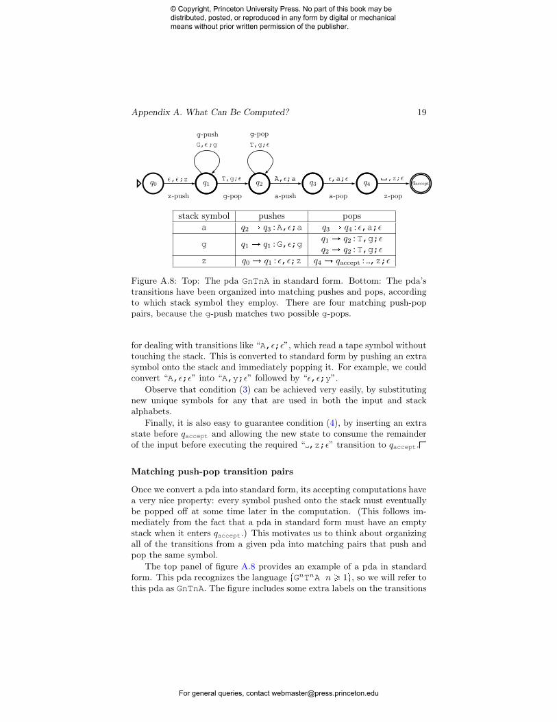
stack symbol pushes popsa q2 Ñ q3 :A,ε;a q3 Ñ q4 : ε,a;ε

g q1 Ñ q1 :G,ε;gq1 Ñ q2 :T,g;εq2 Ñ q2 :T,g;ε

z q0 Ñ q1 : ε,ε;z q4 Ñ qaccept : ,z;ε

Figure A.8: Top: The pda GnTnA in standard form. Bottom: The pda’stransitions have been organized into matching pushes and pops, accordingto which stack symbol they employ. There are four matching push-poppairs, because the g-push matches two possible g-pops.

for dealing with transitions like “A,ε;ε”, which read a tape symbol withouttouching the stack. This is converted to standard form by pushing an extrasymbol onto the stack and immediately popping it. For example, we couldconvert “A,ε;ε” into “A,y;ε” followed by “ε,ε;y”.

Observe that condition (3) can be achieved very easily, by substitutingnew unique symbols for any that are used in both the input and stackalphabets.

Finally, it is also easy to guarantee condition (4), by inserting an extrastate before qaccept and allowing the new state to consume the remainderof the input before executing the required “ ,z;ε” transition to qaccept.l

Matching push-pop transition pairs

Once we convert a pda into standard form, its accepting computations havea very nice property: every symbol pushed onto the stack must eventuallybe popped off at some time later in the computation. (This follows im-mediately from the fact that a pda in standard form must have an emptystack when it enters qaccept.) This motivates us to think about organizingall of the transitions from a given pda into matching pairs that push andpop the same symbol.

The top panel of figure A.8 provides an example of a pda in standardform. This pda recognizes the language tGnTnA |n ¥ 1u, so we will refer tothis pda as GnTnA. The figure includes some extra labels on the transitions




to help with organizing them into matching push-pop pairs. Because thepda is in standard form, we know every transition pushes or pops exactlyone symbol. So it makes sense to describe a transition as, for example, a“g-push” or “z-pop.” In the bottom panel figure A.8, the seven transitionsof the pda have been placed into a table. The transitions are sorted accord-ing to which stack symbol they push or pop; this determines in which row ofthe table each transition is placed. The transitions are further sorted intopushes and pops, and this determines the column for each transition. Fromthe table, we can quickly read off all possible matching pairs of pushes andpops. For example, for the stack symbol a, we see there is exactly one pos-sible matching pair in the top row: the a-push “q2 Ñ q3 :A,ε;a” matchesthe a-pop “q3 Ñ q4 : ε,a;ε”. For the stack symbol g, however, there aretwo possible matching pairs. The g-push “q1 Ñ q1 :G,ε;g” matches eitherof the g-pops “q1 Ñ q2 :T,g;ε” or “q2 Ñ q2 :T,g;ε”.

Clearly, this is a small and simple example. In general, suppose thatfor a given stack symbol x we have k1 x-pushes and k2 x-pops. Then therewould be k1k2 matching pairs of x-pushes and x-pops.

Stack-preserving subcomputations

Given a pda in standard form, an accepting computation of that pda can bethought of as a sequence of legal configurations and transitions beginningin q0 and ending in qaccept with an empty stack. Figure A.9(a) shows an ex-ample of an accepting computation for GnTnA. This example demonstratesour notation for pda computations, which includes the contents of the stackafter each transition, written below the current state. The input tape sym-bol consumed by a transition is written above the arrow between states,and we refer to the string of all of these symbols concatenated togetheras the string consumed by the computation. For example, the acceptingcomputation of figure A.9(a) consumes the string “GGTTA”.

We define a subcomputation to be any sequence of legal consecutive con-figurations and intervening transitions. Figure A.9(b) shows an example,consisting of a sequence of four consecutive states and the intervening tran-sitions, drawn from the accepting computation (a). As before, we definethe string consumed by the subcomputation in the obvious way, in this caseyielding “GTT”. Of course, a string consumed by a subcomputation is notnecessarily in the language recognized by the pda.

Let us now pay attention not to the input symbols consumed, but thebehavior of the stack. Notice how in this particular subcomputation, thestack contains gz at the beginning of the subcomputation and containsz at the end of the subcomputation. Usually, we won’t be interested insubcomputations that alter the stack like this. Instead, we concentrate on




q0εÑ q1

GÑ q1

GÑ q1

TÑ q2

TÑ q2

AÑ q3

εÑ q4 Ñ qaccept

ε z gz

ggz

gz

z az

z ε

(a) an accepting computation for GnTnA

q1GÑ q1

TÑ q2

TÑ q2

gz

ggz

gz

z

(b) a subcomputation for GnTnA

q1GÑ q1

GÑ q1

TÑ q2

TÑ q2

z gz

ggz

gz

z

(c) a stack-preserving subcomputation for GnTnA

Figure A.9: Examples of an accepting computation and subcomputationsfor the GnTnA pda (see figure A.8).




q1GÑ q1

GÑ q1

TÑ q2

TÑ q2

AÑ q3

εÑ q4

z gz

ggz

gz

z az

z

(a) a stack-preserving subcomputation for GnTnA, before splitting

q1GÑ q1

GÑ q1

TÑ q2

TÑ q2

z gz

ggz

gz

zq2

AÑ q3

εÑ q4

z az

z

(b) two stack-preserving subcomputations resulting from splitting (a)

Figure A.10: Example of splitting a stack-preserving subcomputation.

subcomputations that leave the stack undisturbed, and this motivates ournext definition.

A subcomputation is stack-preserving if the initial and final content ofthe stack is identical, and none of the initial content is popped during thesubcomputation. Note that it is not enough for the final content to be thesame as the initial content: we insist that the content remains undisturbed,so it is not permitted to pop any of the initial content during the subcom-putation and replace it before the end. Figure A.9(c) shows an example ofa stack-preserving subcomputation for GnTnA, which consumes the string“GGTT”. Note that any accepting computation automatically satisfies theconditions for being a stack-preserving subcomputation, so figure A.9(a)provides another example. Any single configuration is defined to be a trivialsubcomputation. Because it doesn’t disturb the stack, a trivial subcompu-tation is also stack-preserving.

Splitting and peeling pda subcomputations

Stack-preserving subcomputations can be decomposed into simpler partsvia two operations that we will call splitting and peeling.

We tackle splitting first. Suppose that, at some point before the end ofthe subcomputation, the stack returns to its initial condition. Then we cansplit the subcomputation at that point, creating two shorter subcomputa-tions. The configuration at the point of the split is duplicated, becomingthe end of the first component and the start of the second. Figure A.10gives an example, where we split at the configuration in state q2, when thestack first returns to its initial content z. Note that the components of a




q1GÑ q1

GÑ q1

TÑ q2

TÑ q2

z gz

ggz

gz

z

(a) a stack-preserving subcomputation for GnTnA, before peeling

q1GÑ q1

TÑ q2

gz

ggz

gz

(b) the stack-preserving subcomputation resulting from peeling (a)

Figure A.11: Example of peeling a stack-preserving subcomputation.

split are indeed always stack-preserving, because we split at a point wherethe stack is in its initial condition.

Next, we move on to peeling. We peel a stack-preserving subcompu-tation by removing its first and last configurations. Figure A.11 gives anexample. Note that if we applied the peeling operation a second time inthis example, we would be left with a trivial subcomputation. Obviously,trivial subcomputations cannot be peeled.

It’s worth noting that peeling a stack-preserving subcomputation doesn’talways result in a stack-preserving subcomputation. For example, whatwould happen if we peeled the subcomputation in figure A.10(a)? The re-sulting subcomputation would begin with the stack gz and end with stackaz. And even if the stack had ended with the same content, it’s possiblethat the peeled version could disturb the stack while in one of its intermedi-ate configurations. In fact, the importance of the peeling operation resultsfrom the following property: if a stack-preserving subcomputation can’t besplit, then peeling it will result in another stack-preserving subcomputation.We prove a more precise formulation of this fact in claim A.6 below. Nev-ertheless, it would be a valuable exercise to prove it now, before readingon.

A.5 Converting a pda to a cfg

In this section we complete our proof that pdas and cfgs are equivalent, byshowing that any pda can be converted to an equivalent cfg. We will firstgive an explicit recipe for constructing the cfg; later, we will prove that thiscfg has the desired properties. Given a pda M in standard form, we will




denote the corresponding grammar by GM . We use as a running examplethe case of M � GnTnA, where GnTnA is the pda in figure A.8. To describeGM , we need to describe its variables (including a start variable), terminals,and rules. The terminals are easiest so let’s start there: they consist of M ’sinput alphabet, with the blank symbol excluded. For GnTnA, this meansthe terminals are G, T, and A.

Next we describe the the variables of GM . If GM has k states, thenthere will be k2 variables: one for each ordered pair of states. Let usto denote these by vi,j , where i and j run over all the possible states,including qaccept. For GnTnA, there are 36 variables: v0,0, v0,1, v0,2, . . .,v0,accept, . . ., vaccept,3, vaccept,4, vaccept,accept. Each variable will have avery useful and important interpretation: the variable vi,j will generate allstrings that can be consumed by a stack-preserving subcomputation thatbegins in state qi and ends in state qj . As an example, consider the variablev1,2 in the grammar for GnTnA. This variable will turn out to generate allstrings of the form GnTn. The variable v2,4 will generate only one nonemptystring, “A”. And the variable v1,1 will generate only the empty string.Note that v1,1 will not generate G, GG, GGG, and so on—these strings areconsumed by subcomputations that begin and end at q1, but none of thesesubcomputations is stack-preserving. Is also worth emphasizing at thispoint that this property of the vi,j is something we will have to prove later.It has been mentioned now only to help with understanding and motivation.But note that once we have proved the property, the variable v0,accept willbe particularly important: it will generate all strings that are consumed bystack-preserving subcomputations that begin in q0 and end in qaccept. Inother words, v0,accept will generate precisely the language recognized by M .

Finally we must describe the rules of the grammar GM . There will bea start rule and three other types of rules, which we call split rules, peelrules, and vanishing rules.

The start rule is simple: it takes our usual start symbol s and maps itto v0,accept. And as we just noted above, this will go on to generate thelanguage recognized by M . Formally, we have the rule

sÑ v0,accept.

The split rules are designed to acknowledge the fact that, at least inprinciple, a subcomputation that starts at qi and ends at qj could visitany other state qk on the way. So we need to allow for the possibility ofsplitting such a subcomputation into two components: one from qi to qkand another from qk to qj . Hence, we add all rules of the form

vi,j Ñ vi,kvk,j .




stack symbol pushes popsa q2 Ñ q3 :A,ε;a q3 Ñ q4 : ε,a;ε

g q1 Ñ q1 :G,ε;gq1 Ñ q2 :T,g;εq2 Ñ q2 :T,g;ε

z q0 Ñ q1 : ε,ε;z q4 Ñ qaccept : ,z;ε(a) matching push-pop pairs for GnTnA

v2,4Ñ A v3,3v1,2Ñ G v1,1 Tv1,2Ñ G v1,2 T

v0,acceptÑ v1,4(b) peel rules resulting from the push-pop pairs in (a)

Figure A.12: Example of producing peel rules from matching push-poppairs.

In the example of GnTnA, which has 6 states, this gives us 63 � 216 splitrules. For example, the grammar will contain the rule v1,4 Ñ v1,2v2,4,which will enable the split shown in figure A.10. Note that our constructioncreates many more split rules than necessary. In the GnTnA grammar, forexample, it’s clear that a rule such as v3,1 Ñ v3,2v2,1 is useless, since thereisn’t even a path in the transition graph from q3 to q1. But it turns outthat these useless rules will not affect our proof, and it’s easiest to leavethem in the grammar rather than trying to calculate exactly which oneswill be needed.

The peel rules reflect the fact that some stack-preserving subcomputa-tions can be peeled. Here, we will use the structure of M ’s transitions toensure that only legal peeling operations are reflected in the grammar. Thisis done by creating peel rules only for M ’s matching push-pop transitionpairs, which were described earlier. And if any symbols are consumed bythe peeled transitions, we allow the rule to generate those symbols as ter-minals. The details of how this works can difficult to absorb, so we give anexample first and then proceed to the general definition.

Recall from figure A.8 that we have four matching push-pop transitionpairs for the GnTnA pda. These matching push-pop pairs are reproducedin figure A.12(a), except that non-blank symbols consumed from the inputtape have been highlighted in bold. The four matching pairs lead to fourcorresponding peel rules in the grammar; these are shown in figure A.12(b).For example, the first rule in figure A.12(b) originates from the matchingpair of an a-push and a-pop in the first row of figure A.12(a). We imaginea possible stack-preserving subcomputation that begins with the a-push,




transitioning from q2 to q3 while consuming an A, and ends with the a-pop, transitioning from q3 to q4. We apply the peel operation to thissubcomputation, giving us a new subcomputation that begins in q3 andends in q3. The new subcomputation is represented by v3,3, and its overalleffect will be the same as the original subcomputation, as long as we recordthe fact that an A was consumed at the start. That explains the right-handside of the rule, A v3,3.

Similarly, the second rule in figure A.12(b) originates from the matchingpair consisting of a g-push (q1 Ñ q1) and g-pop (q1 Ñ q2). Peeling thissubcomputation results in a new subcomputation that begins in q1 and endsin q1, but now we recorded the fact that a G was consumed at the start anda T at the end. This yields the right-hand side of the rule, G v1,1 T.

The other rules originate from similar reasoning. The third rule mimicsthe peeling operation shown in figure A.11, for example. One technicality isin the final rule, where consuming a blank symbol is not explicitly recorded.This is a minor detail, but it turns out to be the correct behavior becausewe insist that pdas in standard form consume a blank if and only if theyare transitioning to qaccept.

The general procedure for creating peel rules follows this same pattern.We create a peel rule for every matching push-pop transition pair in M .Specifically, suppose we have a matching pair in which the push transitionsfrom qi to qj while consuming X, and the pop transitions from qk to qlwhile consuming Y . Then we add the following rule to our grammar GM :

vi,l Ñ X vj,k Y.

In the GnTnA example, this leads to the four rules already discussed aboveand listed in figure A.12(b).

Finally, we add the vanishing rules, which reflect the fact that a trivialsubcomputation produces an empty string. So for every state qi, we addthe rule

vi,i Ñ ε.

In the GnTnA example, this gives us the six rules v0,0 Ñ ε, v1,1 Ñ ε, . . ..

Overview of how the cfg operates

At this point, we have not proved anything about the properties of ourgrammar GM . But hopefully it is already intuitively clear how the gram-mar can mimic the operation of the pda M . The idea is that any acceptingcomputation can be broken down into simpler stack-preserving subcompu-tations via splitting and peeling. These operations are applied repeatedlyuntil we are left with only trivial subcomputations, which disappear via




q0εÑ q1

GÑ q1

GÑ q1

TÑ q2

TÑ q2

AÑ q3

εÑ q4 Ñ qaccept

ε z gz

ggz

gz

z az

z ε

(a) a computation accepting the input string “GGTTA”

s Ñ v0,accept use start ruleÑ v1,4 peel the z-push/z-pop pairÑ v1,2 v2,4 split at q2Ñ G v1,2 T v2,4 peel a g-push/g-pop pairÑ GG v1,1 TT v2,4 peel another g-push/g-pop pairÑ GGTT v2,4 eliminate trivial subcomputation at q1Ñ GGTTA v3,3 peel the a-push/a-pop pairÑ GGTTA eliminate trivial subcomputation at q3

(b) derivation of the same string using the corresponding grammar

Figure A.13: Example of mimicking a computation on the pdaM � GnTnA,using the constructed grammar GM

the vanishing rules. As an example, consider the accepting computation byGnTnA in figure A.13(a), which is duplicated from figure A.9(a). This com-putation accepts the input string “GGTTA”. The corresponding grammarcan mimic this computation, as shown by the derivation in figure A.13(b).

Proof that the cfg operates correctly

We have explained how to construct a cfg GM from a pda M that is instandard form. It remains to prove that M and GM are equivalent, i.e.that M accepts a string if and only if GM generates it. However, it isnot easy to prove this directly. Instead, we will prove an even strongerstatement which tells us our interpretation of the symbols vi,j is in factcorrect. In detail, we would like to prove the following claim:

Claim A.6 Let M be a pda in standard form, and let GM be the cfg ob-tained from M via the construction described above, so that GM possessesthe variables vi,j . Then vi,j generates the string of terminals S if and onlyif M has a stack-preserving subcomputation that begins at qi, ends at qj ,and consumes S.

Proof of the claim. We prove this claim by breaking it into two parts:part 1 for the “if” and part 2 for the “only if.” Both parts use the technique




of mathematical induction, which has not been employed elsewhere in thebook, but is required here.

Part 1 of the proof. We assume that M has a stack-preserving subcom-putation that begins at qi, ends at qj , and consumes S; we need to showthat vi,j generates S. We do this by induction on the length L of the sub-computation, where the “length” is the number of transitions followed. It’sworth noting that L is always even, since stack-preserving subcomputationsmust consist of the same number of pushes and pops. The base case of theinduction is a trivial subcomputation, which by definition begins and endsat a single state qi, has no transitions (i.e., L � 0), and consumes only theempty string. Hence, the vanishing rule vi,i Ñ ε guarantees that the basecase holds.

Now we turn to the inductive step. We assume our statement holds forall subcomputations of length at most L � 2, and attempt to prove it forL (which we may assume is even). So, suppose we have a stack-preservingsubcomputation C of even length L ¥ 2 that begins at qi, ends at qj ,and consumes S. There are two cases: either (i) C can be split, or (ii) Ccannot be split. To assist with visualization and understanding, consult theexamples of figure A.10 for case (i) and figure A.11 for case (ii).

Case (i): C can be split, say at qk, producing two smaller stack-preservingsubcomputations: C1 from qi to qk consuming S1, and C2 from qk to qjconsuming S2, where S � S1S2. Both C1 and C2 are strictly shorter thanC, so we can apply the inductive hypothesis to each separately. Hence, wehave that vi,k generates S1 and vk,j generates S2. Finally, by applying thesplit rule vi,j Ñ vi,kvk,j , it follows that vi,j generates S1S2 � S, as desired.

Case (ii): C cannot be split. Let h be the height of the stack when Cbegins and ends. Because C cannot be split, we know the height of thestack is at least h � 1 after every transition except the last. (Otherwise,we could split at the point where the height returned to h.) So the symbolthat C initially pushes onto the stack (say, a) remains undisturbed untilthe very end of the subcomputation, when it is removed by a matching pop.Hence, we can peel this matching pair and the resulting shorter computa-tion will also be stack-preserving (with height at least h � 1 throughoutthe computation). So we will be able to apply the inductive hypothesis tothe peeled computation. In detail, suppose C’s initial a-push transitionsfrom qi to qk consuming X, and suppose C’s final a-pop transitions fromql to qj consuming Y . (Here, X and Y are either ε or symbols from theinput alphabet.) Then peeling C results in a shorter stack-preserving sub-computation C 1 which begins in qk, ends in ql, and consumes S1, where wemust have S � XS1Y . Applying the inductive hypothesis to C 1, we obtainthat vk,l generates S1. Finally, by using the peel rule vi,j Ñ X vk,l Y , we




conclude that vi,j generates XS1Y � S, as desired. (Note that the peel ruleneeded for this is actually present in the grammar, because of the matchinga-push/a-pop pair described above.)

Part 2 of the proof. We assume that vi,j generates S; we need to showthat M has a stack-preserving subcomputation that begins at qi, ends atqj , and consumes S. We do this by induction on the length L of thederivation that generates S, where the “length” is the number of rules thatare applied. For intuition and visualization in the remainder of the proof,consult figure A.13.

First we deal with the base case of the induction. The shortest possiblederivation is a single application of a vanishing rule vi,i Ñ ε, so this is thebase case of the induction with L � 1. The trivial subcomputation at qi isstack-preserving and consumes ε, so the base case holds.

For the inductive step, we assume the statement holds for all derivationsof length less than L, where L ¡ 1. We must show that the statement alsoholds for derivations of length L. The first rule in the derivation is eithera split or peel, and we treat these two cases separately. (Why don’t weconsider the start rule or the vanishing rules? The start rule is irrelevantbecause it doesn’t begin with a variable of the form vi,j . The vanishingrules can occur first only when L � 1. So we are indeed left with only twocases for the first rule: split or peel.)

Case (i): first rule application is a split. The first step must be of theform vi,j Ñ vi,kvk,j , where vi,k generates some string S1, vk,j generatessome string S2, and S � S1S2. The derivations of S1 and S2 are shorterthan L, so we apply the inductive hypothesis to both, concluding that Mhas stack-preserving subcomputations C1, C2 such that C1 goes from qi toqk consuming S1, and C2 goes from qk to qj consuming S2. Concatenatingthese computations together yields a stack-preserving subcomputation fromqi to qj that consumes S1S2 � S, as desired.

Case (ii): first rule application is a peel. Let R denote the peel ruleemployed as the first step of the derivation. So R must be of the form vi,j ÑX vk,l Y , where X and Y are either ε or symbols from the input alphabet.We also know that vk,l generates a string S1 such that S � XS1Y . Thederivation of S1 is shorter than L, so we can apply the inductive hypothesisand conclude that M has a stack-preserving subcomputation C going fromqk to ql and consuming S1. The construction of the grammar guaranteesthat rule R corresponds to a matching push-pop pair for some stack symbol,say a. Therefore, M must possess an a-push that transitions from qi to qkconsuming X, and an a-pop that transitions from ql to qj consuming Y . Wecan concatenate the a-push with the above subcomputation C and the a-pop. This yields the desired stack-preserving subcomputation, completing




the proof. l

Finally, we can tie up the loose ends and use the previous claim tounderstand the entire language generated by GM . In essence, the start ruleyields exactly the desired behavior. The proof below gives the details.

Claim A.7 Let M be a pda in standard form, and let GM be the cfgobtained from M via the construction described above. Then the languageaccepted by M is the same as the language generated by GM .

Proof of the claim. First we show that a string S accepted by M isin the language generated by GM . Since S is accepted by M , there is anaccepting computation that consumes S. By definition, it is in fact a stack-preserving subcomputation that begins at q0 and ends at qaccept. Applyingour previous claim A.6, we conclude that v0,accept generates S. And thestart rule of the grammar, s Ñ v0,accept, produces v0,accept. Hence GMgenerates S.

Next we complete the proof by showing that if S is generated by GM ,then M accepts S. The derivation of S must begin with the start rule,meaning that v0,accept generates S. Applying our previous claim A.6, weconclude that M has a stack-preserving subcomputation that begins at q0,ends at qaccept, and consumes S. This is precisely an accepting computationfor S, and the proof is complete. l

A.6 Summary of computational power of au-tomata

The previous section completed our proof that pdas (or more specifically,npdas) recognize precisely the set of context free languages. As mentionedin section A.1, the strict subset of the cfls recognized by deterministic pdasis known as the deterministic context free languages. Although beyond thescope of this book, the deterministic cfls are of great importance becausethey can be parsed efficiently by compilers.

Figure A.14 combines the results of this chapter with the earlier ones,summarizing which problems and languages can be decided or recognizedby the various computational models we have examined. Models listed inany one row of the table have equivalent computational power, but eachrow is strictly more powerful than the one above. The examples in the lastcolumn demonstrate this by providing examples that cannot be recognizedby the model in the row above.




computationalmodel

languages decidedor recognized

example that can’tbe recognized by

row above

dfa, nfadecide regularlanguages

any regex, e.g., G�T�

dpdadecide deterministiccontext freelanguages

marked palindromes:tGnCTnu

npdarecognize contextfree languages

even palindromes:tGnTnu

tm, ntmdecide any decidablelanguage

tGnTnAnu

Figure A.14: Summary of languages recognized and decided by differentcomputational models.



context free languages and push down automataassets.press.princeton.edu/releases/m11348.pdf ·...

Documents