context e⁄ects - columbia universitymd3405/behave_col_cd_2_16.pdf · a neuroscience primer...

Context Effects

Mark Dean

Behavioral Economics G6943Fall 2016

Context Effects

• We willl now think about context effects that are more generalthan simple reference dependence

• Standard Model: Adding options to a choice set can onlyaffect choice in a very specific way

• Either a new option is chosen or it isn’t• Independence of Irrelevant Alternatives

• Work from economics, neuroscience and psychology suggest adifferent channel

• Change the context of choice• i.e. the distribution of values in a choice set• Adding option x can affect the relative evaluation of y and z• Violation of IIA

Observing Context Effects

• We are going to consider two data sets in which these type ofcontext effects can be observed

1 Stochastic Choice

• Divisive Normalization: Louie, Khaw and Glimcher [2013]

2 Choice between multidimensional alternatives

• Relative Thinking: Bushong, Rabin and Schwartzstein [2015]• Salience: Bordalo, Gennaioli and Shleifer [2012]

• These articles are going to be in a somewhat different style towhat we have seen so far

A Neuroscience Primer

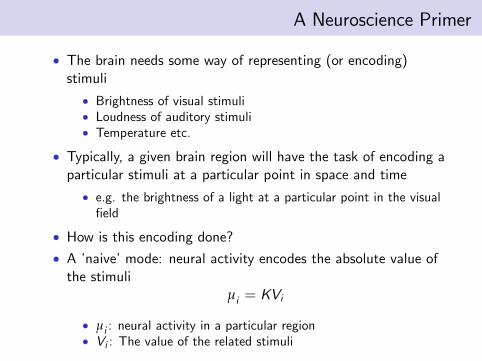
• The brain needs some way of representing (or encoding)stimuli

• Brightness of visual stimuli• Loudness of auditory stimuli• Temperature etc.

• Typically, a given brain region will have the task of encoding aparticular stimuli at a particular point in space and time

• e.g. the brightness of a light at a particular point in the visualfield

• How is this encoding done?• A ’naive’mode: neural activity encodes the absolute value ofthe stimuli

µi = KVi

• µi : neural activity in a particular region• Vi : The value of the related stimuli


• Encoding depends not only on the value of the stimuli, butalso on the context [Carandini 2004]


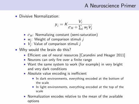
• Divisive Normalization:

µi = KVi

σH +∑j wjVj

• σH : Normalizing constant (semi-saturation)• wj : Weight of comparison stimuli j• Vj : Value of comparison stimuli j

• Why would the brain do this?• Effi cient use of neural resources [Carandini and Heager 2011]• Neurons can only fire over a finite range• Want the same system to work (for example) in very brightand very dark conditions

• Absolute value encoding is ineffi cient• In dark environments, everything encoded at the bottom ofthe scale

• In light environments, everything encoded at the top of thescale

• Normalization encodes relative to the mean of the availableoptions

• Encodes things near the middle of the scale.

Divisive Normalization and Choice

• There is also evidence that the value of choice alternatives isnormalized [Louie et. al. 2011]


• Why should normalization matter for choice?• Does not change the ordering of the valuation of alternatives,so why should it change choice?

• Because choice is stochastic• The above describes mean firing rates• Choice will be determined by a draw from a randomdistribution around that mean

• Claim that such stochasticity is an irreducible fact ofneurological systems

• Probability of choice depends on the difference between theencoded value of each option

• Utility has a cardinal interpretation, not just an ordinal one


• How do these predictions vary from standard random utilitymodel?

• Luce model:p(a|A) = u(a)

∑b∈A u(b)

• Implies that the relative likelihood of picking a over b isindependent of the other available alternatives

• Stochastic IIA

• More general RUM• Adding an alternative c can affect the relative likelihood ofchoosing a and b

• But only because c itself is chosen• Can ‘take away’probability from a or b• The amount c is chosen bounds the effect it can affect thechoice of a or b

Experimental Evidence

• Subjects (40) took part in two tasks involving snack foods

1 Asked to bid on each of 30 different snack foods to elicitvaluation

• BDM procedure used to make things incentive compatible

2 Asked to make a choice from three alternatives

• Target, alternative and distractor• ’True’value of each alternative assumed to be derived fromthe bidding stage

Experimental Evidence

Choice with Multidimensional Alternatives

• In the model we just saw, adding a third ‘distractor’changedthe ‘distance’between the value of two targets

• Context changed apparent magnitude of the difference

• This could not be seen in ’standard’choice data• Is observable in stochastic choice


• Another data set in which such effects could be observed ischoice over goods defined over multiple attributes

• c = {c1, ..., cK }• Utility is assumed additive,

U(c |A) =K

∑k=1

wAk uk (ck )

• uk (.) the true (context independent) utility on dimension k• wAk is a context dependent weight on dimension k

• Utility also assumed to be observable• Koszegi and Szeidl [2013] suggest how this can be done

• Context can change the distance between values on onedimension

• Change the trade off relative to other dimensions


• Many recent papers make use of this framework• Bordalo, Gennaioli and Shleifer [2012, 2013]: Salience• Soltani, De Martino and Camerer [2012]: Range Normalization• Cunningham [2013]: Comparisons• Koszegi and Szeidl [2013]: Focussing• Bushong, Rabin and Schwartzstein [2015]: Relative thinking


• Many recent papers make use of this framework• Bordalo, Gennaioli and Shleifer [2012, 2013]: Salience• Soltani, De Martino and Camerer [2012]: Range Normalization• Cunningham [2013]: Comparisons• Koszegi and Szeidl [2013]: Focussing• Bushong, Rabin and Schwartzstein [2015]: Relative thinking

• We will consider these two

Relative Thinking

• In the Louie et al. [2013] paper, normalization was relative tothe mean of the value of the available options

• There is also a long psychology literature which suggests thatrange can play an important role in normalization

• A given absolute difference will seem smaller if the total rangeunder consideration seems larger

• Bushong et al. [2015] suggest conditions on the weights wAkto capture this effect .

U(c |A) =K

∑k=1

wAk uk (ck )

Relative Thinking: Assumptions

1 wAk = w(∆k (A)) where

∆k (A) = maxa∈A

uk (ak )−mina∈A

uk (ak )

• The weight given to dimension k depends on the range ofvalues in this dimension

2 wAk (∆) is diffable and decreasing in ∆• A given absolute difference receives less weight as the rangeincreases

3 wAk (∆)∆ is strictly increasing, with w(0)0 = 0

• The change in weight cannot fully offset a change in absolutedifference

4 lim∆→∞ w(∆) > 0• Absolute differences still matter even as the range goes toinfinity

Relative Thinking: Implications

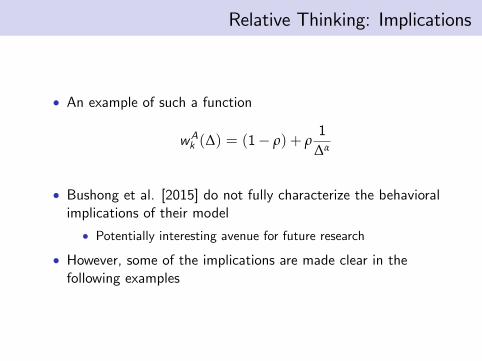
• An example of such a function

wAk (∆) = (1− ρ) + ρ1

∆α

• Bushong et al. [2015] do not fully characterize the behavioralimplications of their model

• Potentially interesting avenue for future research

• However, some of the implications are made clear in thefollowing examples

Example 1

c =

230

, c ′ =005

• Assume these payoffs are in utility units• What will the DM choose?

• They would choose c , despite the fact that the ’unweighted’utility of the two options is the same

2w(2) + 3w(3) > 5w(3) > 5w(5)

• DM favors benefits spread over a large number of dimensions

Example 2

c ={21

}, c ′ =

{12

}• Assume utility is linear• Say that, in the choice set {c , c ′} the DM is indifferentbetween the two.

• What would they choose from

c ={21

}, c ′ =

{12

}, c ′′ =

{20

}• They would choose c• The introduction of c ′′ increases the range of dimension 2,but not dimension 1

• Reduces the weight on the dimension in which c ′ has theadvantage

• This is an example of the asymmetric dominance effect

Example 2

Salience Theory

• Basic Idea: Attention is not spread evenly across theenvironment

• Some things draw our attention whether we like it or not• Bright lights• Loud noises• Funky dancing

• The things that draw our attention are likely to have moreweight in our final decision

• Notice here that attention allocation is exogenous notendogenous

• Potentially could be thought of as a reduced form for someendogenous information gathering strategy

Salience Theory

• Bordalo, Gennaioli and Shleifer [2013] formulate salience inthe following way

U(c |A) =K

∑k=1

wAk ,cuk (ck )

=K

∑k=1

wAk ,c θkck

• θk is the ‘true’utility of dimension k• wAk ,c is the ‘salience’weight of dimension k for alternative c

• Notice that the weight that dimension k receives may bedifferent for different alternatives

Determining Salience

• How are the weights determined?• First define a ’Salience Function’

σ(ck , c̄k )

• c̄k is the reference value for dimension k (usually, but notalways, the mean value of dimension k across all alternatives)

• σ(ck , c̄k ) is the salience of alternative c on dimension k

• Properties of the Salience function1 Ordering: [min(ck , c̄k ),max(ck , c̄k )] ⊃[min(c ′k , c̄

′k ),max(c

′k , c̄′k )]⇒ σ(c ′k , c̄

′k ) ≤ σ(ck , c̄k )

2 Diminishing Sensitivity: σ(ck + ε, c̄k + ε) < σ(ck , c̄k )3 Reflection:

σ(c ′k , c̄′k ) > σ(ck , c̄k )⇒ σ(−c ′k ,−c̄ ′k ) > σ(−ck ,−c̄k )

Determining Salience

• An example of a salience function

σ(ck , c̄k ) =|ck − c̄k ||ck |+ |c̄k |

• Note:• Shares some features with both the previous approaches wehave seen

• Normalization by the mean• Diminishing sensitivity (but relative to zero, rather than therange)

• The precise differences in the behavioral implications betweenthese different models is somewhat murky

From Salience to Decision Weights

• Use σ(ck , c̄k ) to rank the salience of different dimensions forgood c

• rk ,c is the salience rank of dimension k (1 is most salient)

• Assign weight wAk ,c asδrk ,c

∑j θjδrj ,c

• Then plug intoK

∑k=1

wAk ,c θkck

• More salient alternatives get a higher decision weight• δ indexes degree to which subject is affected by salience

• lower δ, more affected by salience

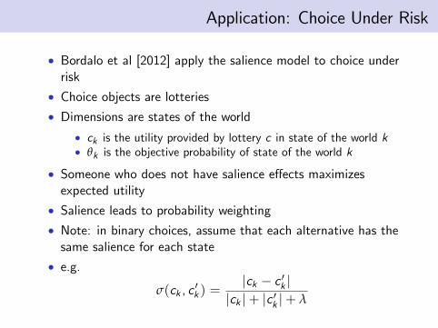
Application: Choice Under Risk

• Bordalo et al [2012] apply the salience model to choice underrisk

• Choice objects are lotteries• Dimensions are states of the world

• ck is the utility provided by lottery c in state of the world k• θk is the objective probability of state of the world k

• Someone who does not have salience effects maximizesexpected utility

• Salience leads to probability weighting• Note: in binary choices, assume that each alternative has thesame salience for each state

• e.g.

σ(ck , c′k ) =

|ck − c ′k ||ck |+ |c ′k |+ λ


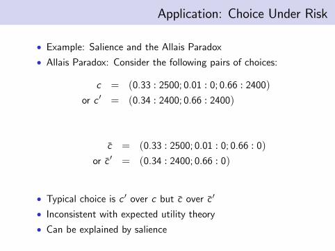
• Example: Salience and the Allais Paradox• Allais Paradox: Consider the following pairs of choices:

c = (0.33 : 2500; 0.01 : 0; 0.66 : 2400)or c ′ = (0.34 : 2400; 0.66 : 2400)

c̄ = (0.33 : 2500; 0.01 : 0; 0.66 : 0)or c̄ ′ = (0.34 : 2400; 0.66 : 0)

• Typical choice is c ′ over c but c̄ over c̄ ′

• Inconsistent with expected utility theory• Can be explained by salience


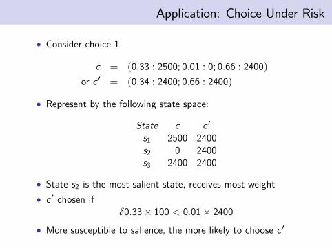
• Consider choice 1

c = (0.33 : 2500; 0.01 : 0; 0.66 : 2400)or c ′ = (0.34 : 2400; 0.66 : 2400)

• Represent by the following state space:

State c c ′

s1 2500 2400s2 0 2400s3 2400 2400

• State s2 is the most salient state, receives most weight• c ′ chosen if

δ0.33× 100 < 0.01× 2400• More susceptible to salience, the more likely to choose c ′


• Consider choice 2

c̄ = (0.33 : 2500; 0.01 : 0; 0.66 : 0)or c̄ ′ = (0.34 : 2400; 0.66 : 0)

• Assume independence and represent by the following statespace:

State c̄ c̄ ′

s1 2500 2400s2 2500 0s3 0 2400s4 0 0

• Salience ranking is s2, then s3, then s1• Now the upside of c̄ is most salient• c̄ ′ chosen if

0.33× 0.66× 2500− δ0.67× 0.34× 2400+ δ20.33× 0.34× 100 < 0• Which is never true for δ ≥ 0

Summary

• There is a large body of evidence which suggests that contexteffects are important in economic choice

• This is a violation of the standard model (via IIA)• A new class of models have tried to explain these effects viathe channel of ‘normalization’

• The context of a choice affects whether a given difference isseen as big or small

• Many open questions in this literature• Type of normalization• What is the ‘context’?• How do we behaviorally differentiate between classes ofmodels?

context e⁄ects - columbia universitymd3405/behave_col_cd_2_16.pdf · a neuroscience primer...

Documents