contents › ddugger › kgeom.pdf(7) (bezout’s theorem) suppose that x,y ,→cp2 are the...
TRANSCRIPT
A GEOMETRIC INTRODUCTION TO K-THEORY
DANIEL DUGGER
Contents
Preface 3
Introduction 41. Algebraic intersection multiplicities 4
Part 1. K-theory in algebra 102. A first look at K-theory 103. A closer look at projectives 204. A brief tour of localization and devissage 235. K-theory of complexes and relative K-theory 296. K-theory of exact complexes 357. A taste of K1 39
Part 2. K-theory in topology 508. Vector bundles 509. Some results from fiberwise linear algebra 6010. Swan’s Theorem 6411. Homotopy invariance of vector bundles 6712. Vector bundles on spheres 7213. Topological K-theory 7714. Vector fields on spheres 83
Part 3. K-theory and geometry I 9415. The Thom isomorphism for singular cohomology 9416. Thom classes and intersection theory 10117. Thom classes in K-theory 10718. The denouement: connecting algebra, topology, and geometry 11719. More about relative K-theory 125
Part 4. K-theory and geometry II 13920. K∗(CPn) and the K-theoretic analog of the degree 13921. Interlude on the calculus of finite differences 14722. The Euler class 15323. Chern classes 16524. Comparing K-theory and singular cohomology 16925. The Grothendieck-Riemann-Roch Theorem 17626. The algebro-geometric GRR theorem 18827. Formal group laws and complex-oriented cohomology theories 191
1
2 DANIEL DUGGER
28. Algebraic cycles on complex varieties 191
Part 5. Topological techniques and applications 20129. The Atiyah-Hirzebruch spectral sequence 20130. Operations on K-theory 21731. The Hopf invariant one problem 22432. Calculation of KO for stunted projective spaces 23633. Solution to the vector field problem 25234. The immersion problem for RPn 26335. The sums-of-squares problem and beyond 274
Part 6. Homological intersection theory 28436. The theorem of Gillet-Soule 284
Part 7. Appendices 284Appendix A. Bernoulli numbers 284Appendix B. The algebra of symmetric functions 287Appendix C. Homotopically compact pairs 289References 291
A GEOMETRIC INTRODUCTION TO K-THEORY 3
Preface
I first learned Serre’s definition of intersection multiplicity from Mel Hochster,back when I was an undergraduate. I was immediately intrigued by this surprisingconnection between homological algebra and geometry. As it has always been forme when learning mathematics, I wanted to know how I could have guessed thisdefinition for myself—what are the underlying principles that tell us to go lookingin homological algebra for a definition of multiplicity. This question has been in theback of my mind for most of my mathematical life. It took me a long time to acceptthat the answers to such questions are not often readily available; one has to insteadmake do with vague hints and partial explanations. I still believe, though, that theanswers exist somewhere—and that it is the ultimate job of mathematicians touncover them. So perhaps it is better said this way: those questions often don’thave simple answers yet .
During my first year of graduate school I tried to puzzle out for myself the secretsbehind Serre’s definition. Thanks to the Gillet-Soule paper [GS] I was led to K-theory, and similar hints of topology seemed to be operating in work of Roberts [R].Coincidentally, MIT had a very active community of graduate students in topology,and I soon joined their ranks. Although there were other factors, it is not far fromthe truth to say that I became a topologist in order to understand Serre’s definition.
In Winter quarter of 2012 I taught a course on this material at the Universityof Oregon. The graduate students taking the course converted my lectures intoLaTeX, and then afterwards I both heavily revised and added to the resultingdocument. The present notes are the end result of this process. I am very gratefulto the attending graduate students for the work they put into typesetting thelectures. These students were: Jeremiah Bartz, Christin Bibby, Safia Chettih,Emilio Gardella, Christopher Hardy, Liz Henning, Justin Hilburn, Zhanwen Huang,Tyler Kloefkorn, Joseph Loubert, Sylvia Naples, Min Ro, Patrick Schultz, MichaelSun, and Deb Vicinsky.
4 DANIEL DUGGER
Introduction
1. Algebraic intersection multiplicities
Let Z be the parabola y = x2 in R2, and let W be the tangent line at thevertex: the line y = 0. Then Z and W have an isolated point of intersection at(0, 0). Since high school you have known how to associate a multiplicity with thisintersection: it is multiplicity 2, essentially because the polynomial x2 has a doubleroot at x = 0. This multiplicity also has a geometric interpretation, coming fromintersection theory. If you perturb the intersection a bit, say by moving either Zor W by some small amount, then you get two points of intersection that are near(0, 0)—and these points both converge to (0, 0) as the perturbation gets smallerand smaller.
You might object, rightly so, that I am lying to you. If we perturb y = 0 to y = ε,with ε > 0, then indeed we get two points of intersection: (
√ε, ε) and (−
√ε, ε). And
these do indeed converge to (0, 0) as ε→ 0. But if we perturb the line in the otherdirection, by taking ε to be negative, then we get no points of intersection at all!To fix this, it is important to work over the complex numbers rather than the reals:the connection between geometry and algebra works out best (and simplest) in thiscase. If we work over C, then it is indeed true that almost all small perturbationsof our equations yield two solutions close to (0, 0).
Our goal will be to vastly generalize the above phenomenom. Let f1, . . . , fk ∈C[x1, . . . , xn], and let Z be the algebraic variety defined by the vanishing of thefj ’s. We write
Z = V (f1, . . . , fk) = x ∈ Cn | f1(x) = f2(x) = · · · = fk(x) = 0.Likewise, let g1, . . . , gl ∈ C[x1, . . . , xn] and let W = V (g1, . . . , gl). Assume that Pis an isolated point of the intersection Z∩W . Our goal is to determine an algebraicformula, in terms of the fi’s and gj ’s, for an intersection multiplicity i(Z,W ;P ).This multiplicity should have the basic topological property that it coincides withthe number of actual intersection points under almost all small deformations of Zand W .
Here are some basic properties, by no means comprehensive, that we would wantsuch a formula to satisfy:(1) i(Z,W ;P ) should depend only on local information about Z and W near P .(2) i(Z,W ;P ) ≥ 0 always.(3) If dimZ+dimW < n then i(Z,W ;P ) = 0 (because in this case there is enough
room in the ambient space to perturb Z and W so that they don’t intersect atall).
(4) If dimZ + dimW = n then i(Z,W ;P ) > 0.(5) If dimZ + dimW = n and Z and W meet transversely at P (meaning that
TPZ ⊕ TPW = Cn), then i(Z,W ;P ) = 1.Note that because of property (1) we can extend the notion of intersection mul-
tiplicity to varieties in CPn, simply by looking locally inside an affine chart forprojective space that contains the point P . From now on we will do this withoutcomment. The two statements below are not exactly ‘basic properties’ along thelines of (1)–(5) above, but they are basic results that any theory of intersectionmultiplicities should yield as consequences.
A GEOMETRIC INTRODUCTION TO K-THEORY 5
(6) Suppose that X → CPn is the vanishing set of a homogeneous polynomial,that is X = V (f). Let L be a projective line in CPn that meets X infinitely-many points. Then∑
P∈X∩Li(X,L;P ) = deg(f).
(7) (Bezout’s Theorem) Suppose that X,Y → CP 2 are the vanishing sets ofhomogeneous polynomials f and g, and that X∩Y consists of finitely-manypoints. Then ∑
P∈X∩Yi(X,Y ;P ) = (deg f)(deg g).
Note that (6), for the particular case n = 2, is a special case of (7).If you play around with some simple examples, an idea for defining intersection
multiplicities comes up naturally. It is
i(Z,W ;P ) = dimC
[C[x1, . . . , xn]/(f1, . . . , fk, g1, . . . , gl)
]P.(1.1)
Here the subscript P indicates localization of the given ring at the maximal ideal(x1−p1, . . . , xn−pn) where P = (p1, . . . , pn). The localization is necessary becauseZ∩W might have points other than P in it, and our definition needs to only dependon what is happening near P .
The best way to get a feeling for the above definition is via some easy examples:
Example 1.2. Let f = y−x2 and g = y. This is our example of the parabola andthe tangent line at its vertex. The point P = (0, 0) is the only intersection point,and our definition tells us to look at the ring
C[x, y]/(y − x2, y) ∼= C[x]/(x2).
As a vector space over C this is two-dimensional, with basis 1 and x. So ourdefinition gives i(Z,W ;P ) = 2 as desired. [Note that technically we should localizeat the ideal (x, y), which corresponds to localization at (x) in C[x]/(x2); however,this ring is already local and so the localization has no effect].
Example 1.3. Let f = y2 − x3 − 3x and g = y − 32x −
12 . Then Z = V (f) is an
elliptic curve, and one can check that W = V (g) is the tangent line at the pointP = (1, 2). Let us recall how this works: the gradient vector to the curve is
∇f = [−3x2 − 3, 2y]
and this is normal to the curve at (x, y). A tangent vector is then [2y, 3x3 + 3](since this is orthogonal to ∇f), which means the slope of the curve at (x, y) is(3x3 + 3)/2y. At the point (1, 2) we then get slope 3
2 , and V (g) is the line passingthrough (1, 2) with this slope.
The line V (g) intersects the curve at one other point, which we find by simulta-neously solving y2 = x3 + 3x and y = 3
2x+ 12 . This yields the cubic
0 = x3 + 3x− ( 32x+ 1
2 )2.
Since we know that x = 1 is a root, we can factor this out and then solve theresulting quadratic. One finds that the cubic factors as
0 = (x− 1)2 · (x− 14 ).
The second point of intersection is found to be Q = (14 ,
78 ).

6 DANIEL DUGGER
Note the appearance of (x− 1) with multiplicity two in the above factorization.The fact that we had a tangent line at x = 1 guaranteed that the multiplicitywould be strictly larger than one. Likewise, the fact that (x − 1
4 ) has multiplicityone tells us that V (g) intersects the curve transversally. These facts suggest thati(Z,W ;P ) = 2 and i(Z,W ;Q) = 1. Let us consider these in terms of point-countingunder small deformations. We can perturb either Z or W , but it is perhaps easiestto perturb the line W : we can write g′ = y − Ax − B and then consider whathappens for all (A,B) near ( 3
2 ,12 ). We will need to find the intersection of Z and
W ′ = V (g′), which as before leads to a cubic. To save us from the unpleasantnessof having to solve the cubic, let us again arrange for there to be a known solutionwhich we can factor out. It is possible to have this solution be either (1, 2) or (1
4 ,78 ).
The calculations turn out to be a little easier for the latter, despite the annoyingfractions. So we assume 7
8 = A4 + B, or g′ = y − A(x − 1
4 ) − 78 . Since we want to
look at A near 32 , it is convenient to write A = 3
2 + ε where ε is near zero.Finding common solutions of f = 0 and g′ = 0 yields a cubic with (x− 1
4 ) as afactor, and dividing this out we obtain the quadratic
0 = x2 − x(2 + 3ε+ ε2) + (1− ε+ ε2
4 ).
The discriminant of this quadratic is D = ε(ε3 +6ε2 +4ε+16), so the quadratic hasa double root when ε = 0 (as expected) but simple roots for values of ε near butnot equal to zero. So for these values of ε we get two points of intersection of V (f)and V (g′) near P , and it is easy to see that they converge to P as ε approacheszero.
Let us now see what our provisional definition from (1.1) gives. The quotientring in our definition is
C[x, y]/(y2 − x3 − 3x, y − 3
2x−12
) ∼= C[x]/(( 32x+ 1
2 )2 − x3 − 3x)
∼= C[x]/((x− 1)2(x− 1
4 )).
Here we are killing a cubic in C[x], and so we get a three-dimensional vector spacewith basis 1, x, x2. Note that this is, in some sense, seeing all of the information atP and Q together—this demonstrates the importance of localization. Localizationat P corresponds to localizing at (x − 1), which turns (x − 1
4 ) into a unit. So ourlocalized ring is
C[x](x−1)/((x− 1)2) ∼= C[t](t)/(t2)(where we set t = x − 1), and this has dimension 2 over C. So i(Z,W ;P ) = 2, asdesired.
If we localize at (x− 14 ) then the (x− 1)2 factor becomes a unit, and our local-
ized ring becomes C[x](x− 14 )/(x − 1
4 ) ∼= C[t](t)/(t), which is just a copy of C. Soi(Z,W ;Q) = 1.
Note that both Example 1.2 and Example 1.3 involve a key step where thevariable y is eliminated, thus bringing the problem down to the multiplicity of aroot in a one-variable polynomial. One cannot always do such an elimination—infact it happens only rarely. So these examples are very special, although they stillserve to give some sense of how things are working.
It turns out that our provisional definition from (1.1) is enough to prove Bezout’sTheorem for curves in CP 2. But in some sense one is getting lucky here, and itworks only because the dimensions of the varieties are so small. When one starts
A GEOMETRIC INTRODUCTION TO K-THEORY 7
to look at higher-dimensional varieties it doesn’t take long to find examples wherethe definition clearly gives the wrong answers:
Example 1.4. Let C4 have coordinates u, v, w, y, and let X,Y ⊆ C4 be given by
X = V (u3 − v2, u2y − vw, uw − vy, w2 − uy2), Y = V (u, y).
Note that X is somewhat complicated, but Y is just a plane. If a point (u, v, w, y)is on X ∩ Y then u = y = 0 and therefore the equations for X say that
v2 = 0, vw = 0, and w2 = 0
as well. So X ∩Y consists of the unique point (0, 0, 0, 0). Our provisional definitionof intersection multiplicities would have us look at the ring
C[u, v, w, y]/(u, y, u3 − v2, u2y − vw, uw − vy, w2 − uy2) ∼= C[v, w]/(v2, vw,w2)
which is three-dimensional over C. If this were the correct answer, then perturbingthe plane Y should generically give three points of intersection. However, this isnot the case. If we perturb Y to V (x − ε, y − δ) then the intersection with X isgiven by the equations
u = ε, y = δ, ε3 = v2, ε2δ = vw, εw = vδ, w2 = εδ2.
As long as ε 6= 0 we have two solutions for v, and then the fourth equation deter-mines w completely. So we only have two points on the intersection, after smallperturbations. This is, in fact, the correct answer: i(Z,W ;P ) = 2, and our provi-sional definition is a failure.
Serre discovered the correct formula for the interesection multiplicity [S]. Hisformula is as follows. If we set R = C[x1, . . . , xn] then
i(Z,W ;P ) =∞∑j=0
(−1)j dimC
[TorRj
(R/(f1, . . . , fk), R/(g1, . . . , gl)
)]P.(1.5)
There are several things to say here. First, although the sum is written to infinityit turns out that the Tor modules vanish for all j > n (we will prove this later). Soit is, in fact, a finite sum. Secondly, the condition that P be an isolated point ofintersection forces the C-dimension of all the Tor’s to be finite. So the formula doesmake sense. As to why this gives the “correct” numbers, it will take us a while toexplain this. But note that the j = 0 term is the dimension of
Tor0(R/(f1, . . . , fk), R/(g1, . . . , gl)) ∼= R/(f1, . . . , fk)⊗R R/(g1, . . . , gl)∼= R/(f1, . . . , fk, g1, . . . , gl).
So our provisional definition from (1.1) is just the j = 0 term. One should thinkof the higher terms as “corrections” to this initial term; in a certain sense thesecorrections get smaller as j increases (this is not obvious).
An algebraist who looks at (1.5) will immediately notice some possible gener-alizations. The R/(f) and R/(g) terms can be replaced by any finitely-generatedmodule M and N , as long as the Torj(M,N) modules are finite-dimensional overC. For this it turns out to be enough that M ⊗R N be finite-dimensional overC. Also, we can replace C[x1, . . . , xn] with any ring having the property that allfinitely-generated modules have finite projective dimension—necessary so that thealternating sum of (1.5) is finite. Such rings are called regular. Also, instead oflocalizing the Tor-modules we can just localize the ring R at the very beginning.
8 DANIEL DUGGER
And finally, in this generality we need to replace dimC with a similar invariant: thenotion of length (meaning the length of a composition series for our module). Thisleads to the following setup.
Let R be a regular, local ring (all rings are assumed to be commutative andNoetherian unless otherwise noted). Let M and N be finitely-generated modulesover R such that M ⊗R N has finite length. This implies that all the Torj(M,N)modules also have finite length. Define
e(M,N) =∞∑j=0
(−1)j`(Torj(M,N)
)(1.6)
and call this the intersection multiplicty of the modules M and N .Based on geometric intuition, Serre made the following conjectures about the
above situation:(1) dimM + dimN ≤ dimR always(2) e(M,N) ≥ 0 always(3) If dimM + dimN < dimR then e(M,N) = 0.(4) If dimM + dimN = dimR then e(M,N) > 0.Serre proved all of these in the case that R contains a field, the so-called “geometriccase” (some non-geometric examples for R include power series rings over the p-adic integers Zp). Serre also proved (1) in general. Conjecture (3) was proven inthe mid 80s by Roberts and Gillet-Soule (independently), using some sophisticatedtopological ideas that were imported into algebra. Conjecture (2) was proven byGabber in the mid 90s, using some high-tech algebraic geometry. Conjecture (4) isstill open.
1.7. Where we are headed. Our main goal in these notes is to describe a par-ticular subset of the mathematics surrounding Serre’s definition of multiplicity. Itis possible to explore this subject purely in algebraic terms, and that is basicallywhat Serre did in his book [S]. In contrast, our main focus will be topological.Although both commutative algebra and algebraic geometry play a large role inour story, we will always adopt a perspective that concentrates on their relationsto topology—and in particular, to K-theory.
Here is a brief summary of some of the main points that we will encounter:(1) There are certain generalized cohomology theories—called complex-oriented—
which have a close connection to geometry and intersection theory. Any suchcohomology can be used to detect intersection multiplicities.
(2) Topological K-theory is a complex-oriented cohomology theory. Elements ofthe groups K∗(X) are specified by vector bundles on X, or more generally bybounded chain complexes of vector bundles on X. Fundamental classes forcomplex submanifolds of X are given by resolutions.
(3) When X is an algebraic variety there is another version of K-theory calledalgebraic K-theory , which we might denote K∗
alg(X). The analogs of vectorbundles are locally free coherent sheaves, or just finitely-generated projectivemodules when X is affine. Thus, in the affine case elements of K∗
alg(X) can bespecified by bounded chain complexes of finitely-generated projective modules.This is the main connection between homological algebra and K-theory.
A GEOMETRIC INTRODUCTION TO K-THEORY 9
(4) Serre’s definition of intersection multiplicities essentially comes from the inter-section product in K-homology, which is the cup product in K-cohomologytranslated to homology via Poincare Duality.
We will spend a large chunk of these notes filling in the details behind (1)–(4).But whereas we take our motivation from Serre’s definition of multiplicity, that isnot the only subject we cover in these notes. Once we have the K-theory apparatusup and running, there are lots of neat things to do with it. We have attempted, forthe most part, to chose topics that accentuate the relationship between K-theoryand geometry in the same way that Serre’s definition of multiplicity does.
10 DANIEL DUGGER
Part 1. K-theory in algebra
In this first part of the notes we investigate the K-theory of modules over aring R. There are two main varieties: one can study the K-theory of all finitely-generated modules, leading to the group G(R), or one can study the K-theory offinitely-generated projective modules—leading to the group K(R). In the followingsections we get a taste for these groups and the relations between them.
For the duration of these notes, all rings are commutative with identity unlessotherwise stated. Some of the theory we develop works in greater generality, butwe will stay focused on the commutative case.
2. A first look at K-theory
Understanding Serre’s alternating-sum-of-Tor’s formula for intersection multi-plicities will be a gradual process. In particular, there is quite a bit of nontrivialcommutative algebra that is needed for the story; we will need to develop this aswe go along. We will continue to sweep some of these details under the rug for themoment, but let us at least get a couple of things out in the open. To begin with,we will need the following important result:
Theorem 2.1 (Hilbert Syzygy Theorem). Let k be a field and let R be k[x1, . . . , xn](or any localization of this ring). Then every finitely-generated R-module has a freeresolution of length at most n.
We will prove this theorem in Section 17 below. We mention it here because itimplies that Torj(M,N) = 0 for j > n. Therefore the sum in Serre’s formula isactually finite. More generally, a ring is called regular if every finitely-generatedmodule has a finite, projective resolution. It is a theorem that localizations of regu-lar rings are again regular. Hilbert’s Syzygy Theorem simply says that polynomialrings over a field are regular. We will find that regular rings are the ‘right’ contextin which to explore Serre’s formula.
We will also need the following simple observation. If P is a prime ideal in anyring R, then
[TorR(M,N)]P = TorRp(MP , NP ).To see this, let Q• → M → 0 be an R-free resolution of M . Since localization isexact, (Q•)P is an RP -free resolution of MP . Hence
TorRPj (MP , NP ) = Hj
((Q•)P ⊗RP
NP)
= Hj
(Q• ⊗R RP ⊗RP
N ⊗R RP)
= Hj
(Q• ⊗R N ⊗RP
)= Hj
(Q• ⊗R N
)⊗RP
= TorRj (M,N)⊗R RP .The importance of this observation is that it tells us that the Tor’s in Serre’s formulamay all be taken over the ring RP . So we might as well work over this ring frombeginning to end. Moreover, without loss of generality we might as well assumethat our point of intersection is the origin, which makes the corresponding maximalideal (x1, . . . , xn).
Let R = C[x1, . . . , xn](x1,...,xn), and let M and N be finitely-generated modulesover R. Assume that dimC(M ⊗R N) < ∞. It turns out that this implies that
A GEOMETRIC INTRODUCTION TO K-THEORY 11
dimC Torj(M,N) <∞ for every j, so that we can define
e(M,N) =∞∑j=0
(−1)j dimC Torj(M,N).
The above definition generalizes the notion of intersection multiplicity from pairs(R/I,R/J) to pairs of modules (M,N). The reason for making this generalizationmight not be clear at first, but the following nice property provides some justifica-tion:
Lemma 2.2. Suppose that 0→ M ′ → M → M ′′ → 0 is a short exact sequence ofR-modules. Then e(M,N) = e(M ′, N)+e(M ′′, N), assuming all three multiplicitiesare defined (that is, under the assumption that dimC(M ⊗ N) < ∞ and similarlywith M replaced by M ′ and M ′′).
Proof. Consider the long exact sequence
· · · → Torj(M ′, N)→ Torj(M,N)→ Torj(M ′′, N)→ · · ·This sequence terminates after a finite number of steps, by Hilbert’s Syzygy Theo-rem. By exactness, the alternating sum of the dimensions is zero. This is preciselythe desired formula.
Lemma 2.2 is referred to as the additivity of intersection multiplicities. Of coursethe additivity holds equally well in the second variable, by the same argument.
While exploring ideas in this general area, Grothendieck hit upon the idea of in-venting a group that captures all the additive invariants of modules. Any invariantsuch as e(−, N) would then factor through this group. Here is the definition:
Definition 2.3. Let R be any ring. Let F(R) be the free abelian group with one gen-erator [M ] for every isomorphism class of finitely-generated R-module M . Let G(R)be the quotient of F(R) by the subgroup generated by all elements [M ]− [M ′]− [M ′′]for every short exact sequence 0 → M ′ → M → M ′′ → 0 of finitely-generated R-modules. The group G(R) is called the Grothendieck group of finitely-generatedR-modules.
Remark 2.4. It is important in the definition of G(R) that one use only finitely-generated R-modules, otherwise the group would be trivial. To see this, if M is anymodule then let M∞ = M ⊕M ⊕M · · · . Note that there is a short exact sequence
0→M →M∞ →M∞ → 0
where M is included as the first summand. If we had defined G(R) without thefinite-generation condition, we would have [M∞] = [M ] + [M∞] and therefore[M ] = 0. Since this holds for every module M , the group G(R) would be zero.This is called the “Eilenberg Swindle”.
The following lemma records some useful ways of obtaining relations in G(R):
Lemma 2.5. Let R be any ring.(a) If 0 → Cn → Cn−1 → · · · → C1 → C0 → 0 is an exact sequence of finitely-
generated R-modules, then∑
(−1)i[Ci] = 0 in G(R).(b) If M = M0 ⊇ M1 ⊇ M2 ⊇ · · · ⊇ Mn ⊇ Mn+1 = 0 is a filtration of M by
finitely-generated modules, then [M ] =∑i[Mi/Mi+1] in G(R).
12 DANIEL DUGGER
(c) Assume that R is Noetherian, and let 0→ Cn → Cn−1 → · · · → C1 → C0 → 0be any chain complex of R-modules. Then
∑i(−1)i[Ci] =
∑i(−1)i[Hi(C)] in
G(R).
Proof. We prove (a) and (c) at the same time. If C• is a chain complex, note thatone has the short exact sequences 0 → Zi → Ci → Bi−1 → 0 where Zi and Biare the cycles and boundaries in each dimension. One also has 0 → Bi → Zi →Hi(C) → 0. Assuming everything in sight is finitely-generated, one gets a seriesof relations in G(R) that immediately yield
∑(−1)i[Ci] =
∑(−1)i[Hi(C)]. So if
R is Noetherian we are done, because everything indeed is finitely-generated; thisproves (c). In the general case where R is not necessarily Noetherian, we know thateach Bi is finitely-generated because it is the image of Ci+1. But if C• is exactthen Bi = Zi and so the Zi’s are also finitely-generated. We have the relations[Ci] = [Zi]+[Bi−1] = [Zi]+[Zi−1], and from this it is evident that
∑(−1)i[Ci] = 0.
This proves (a).The proof of (b) is similarly easy; one considers the evident exact sequences
0→Mi+1 →Mi →Mi/Mi+1 → 0 and the resulting relations in G(R).
Here are a series of examples:(1) Suppose R = F , a field. Clearly G(F ) is generated by [F ], since every finitely-
generated F -module has the form Fn. If we observe the existence of the grouphomomorphism dim: G(F ) → Z, which is clearly surjective because it sends[F ] to 1, then it follows that G(F ) ∼= Z.
(2) More generally, suppose that R is a domain. The rank of an R-module M isdefined to be the dimension of M ⊗RQF (R) over QF (R), where QF (R) is thequotient field. The rank clearly gives a homomorphism G(R) → Z, which issurjective because [R] 7→ 1. So G(R) has Z as a direct summand.
(3) Next consider R = Z. Then G(Z) is generated by the classes [Z] and [Z/n]for n > 1, by the classification of finitely-generated abelian groups. The shortexact sequence 0 → Z n−→ Z −→ Z/n → 0 shows that [Z/n] = 0 for all n,hence G(Z) is cyclic. Using (b), it follows that G(Z) = Z. This computationworks just as well for any PID.
(4) So far we have only seen cases where G(R) ∼= Z. For a case where this is nottrue, try R = F × F where F is a field. You should find that G(R) ∼= Z2 here.
(5) Let G be a finite group, and let R = C[G] be the group algebra. So R-modulesare just representations of G on complex vector spaces. The basic theory of suchfinite-dimensional representations says that each is a direct sum of irreducibles,in an essentially unique way. Moreover, each short exact sequence is split. Alittle thought shows that this is saying that G(R) is a free abelian group withbasis consisting of the isomorphism classes of irreducible representations.
(6) So far all the examples we have computed have G(R) equal to a free abeliangroup. This is not always the case, although I don’t know an example whereit is really easy to see this. For a not-so-simple example, let R be the ring ofintegers in a number field. It turns out that G(R) ∼= Z ⊕ Cl(R), where Cl(R)is the ideal class group of R. This class group contains some sophisticatednumber-theoretic information about R. It is known to always be torsion, andit is usually nontrivial. We will work out a simple example when we have moretools under out belt: see Example 4.2.
A GEOMETRIC INTRODUCTION TO K-THEORY 13
(7) As another simple example, we look at R = F [t]/(t2) where F is a field. For anymodule M over R we have the filtration M ⊇ tM , and so [M ] = [M/tM ]+[tM ].But both M/tM and tM are killed by t, hence are direct sums of copies of F(where t acts as zero). This shows that G(R) is generated by [F ]. We also havethe function dimF (−) : G(R) → Z. Since this function sends [F ] to 1, it mustbe an isomorphism.
(8) The final example we consider here is a variation of the previous one. Let uslook at R = Z/p2. The R-modules are simply abelian groups killed by p2.Given any such module A one can consider the sequence 0 → pA → A →A/pA → 0, and observe that the first and third terms are Z/p-vector spaces.So [Z/p] generates G(R). We claim that G(R) ∼= Z, and as in the previousexample the easiest way to see this is to write down an additive invariant ofR-modules taking its values in Z. All finitely-generated R-modules have a finitecomposition series, and so we can take the Jordan-Holder length; this is thesame as `(A) = dimZ/pA/pA + dimZ/p pA. With some trouble one can checkthat this is indeed an additive invariant (or refer to the Jordan-Holder theorem),and of course `(Z/p) = 1. This completes the calculation.
Exercise 2.6. Prove that G(R) ∼= Z for R = F [t]/(tn) or R = Z/pn.
The above examples help establish some basic intuition. In general, though, itis very hard to compute G(R).
We can adapt our definition of intersection multiplicity of two modules to definea product on G(R), at least when R is regular. For finitely-generated modules Mand N , define
[M ] [N ] =∑j
(−1)j [Torj(M,N)].
The long exact sequence for Tor shows that this definition is additive in the twovariables, and hence passes to a pairing G(R)⊗G(R)→ G(R). It is not at all clearthat this is associative, although we will prove this shortly.
The above product on G(R) is certainly not the first thing one would think of.It is more natural to try to define a product by having [M ] · [N ] = [M⊗RN ], but ofcourse this is not additive in the two variables because of the failure of the tensorproduct to be exact. The higher Tor’s are correcting for this. However, we canmake this naive definition work if we restrict to a certain class of modules. To thatend, let us introduce the following definition:
Definition 2.7. Let R be any ring. Let FK(R) be the free abelian group withone generator [P ] for every isomorphism class of finitely-generated, projective R-module M . Let K(R) be the quotient of FK(R) by the subgroup generated by allelements [P ]− [P ′]− [P ′′] for every short exact sequence 0→ P ′ → P → P ′′ → 0 offinitely-generated projectives. The group K(R) is called the Grothendieck groupof finitely-generated projective modules.
Every short exact sequence of projectives is actually split, so we could also havedefined K(R) by imposing the relations [P ⊕Q] = [P ] + [Q] for every two finitely-generated projectives P and Q. This makes it a little easier to understand whentwo modules represent the same class in K(R):

14 DANIEL DUGGER
Proposition 2.8. Let P and Q be finitely-generated projective R-modules. Then[P ] = [Q] in K(R) if and only if there exists a finitely-generated projective moduleW such that P ⊕W ∼= Q⊕W . In fact, the same remains true if we require W tobe free instead of projective.
Proof. The ‘if’ part of the proposition is trivial; we concentrate on the ‘only if’part. Let Rel ⊆ F(R) be the subgroup generated by all elements [J ] − [J ′] − [J ′′]for short exact sequences 0 → J ′ → J → J ′′ → 0. If [P ] − [Q] ∈ Rel then thereexists two collections of such sequences 0 → P ′i → Pi → P ′′i → 0, 1 ≤ i ≤ k1, and0→ Q′i → Qi → Q′′i → 0, 1 ≤ i ≤ k2, such that
[P ]− [Q] =k1∑i=1
([Pi]− [P ′i ]− [P ′′i ]
)+
k2∑i=1
([Q′i] + [Q′′i ]− [Qi]
)in F(R). Rearranging, this gives
[P ] +k1∑i=1
([P ′i ] + [P ′′i ]
)+
k2∑i=1
[Qi] = [Q] +k1∑i=1
[Pi] +k2∑i=1
([Q′i] + [Q′′i ]
).
The only way such sums of basis elements can give the same element of F(R) is ifthe collection of summands on the two sides are the same up to permutation. Butin that case one can write
P ⊕k1⊕i=1
(P ′i ⊕ P ′′i
)⊕
k2⊕i=1
Qi ∼= Q⊕k1⊕i=1
Pi ⊕k2⊕i=1
(Q′i ⊕Q′′i
).
But note that Pi ∼= P ′i ⊕ P ′′i and similarly for Qi. So if we let W be the module⊕k1i=1
(P ′i ⊕ P ′′i )⊕
⊕k2i=1Qi then we have P ⊕W ∼= Q⊕W .
For the last statement in the proposition, just observe that since W is projectiveit is a direct summand of a free module. That is, there exists a module W ′ such thatW⊕W ′ is finitely-genereated and free. Certainly P⊕(W⊕W ′) ∼= Q⊕(W⊕W ′).
Since projective modules are flat, the product [P ] · [Q] = [P ⊗RQ] is additive andso extends to a product K(R)⊗K(R)→ K(R). Note that this product is obviouslyassociative, and so makes K(R) into a ring. This is true without any assumptionson R whatsoever (except our standing assumption that R be commutative).
Remark 2.9. Given the motivation of having the tensor product give a ring struc-ture, one might wonder why we used projective modules to define K(R) rather thanflat modules. We could have done so, but for finitely-generated modules over com-mutative, Noetherian rings, being flat and projective are equivalent notions—see[E, Corollary 6.6]. For various reasons it is more common to make the definitionusing the projective hypothesis.
There is an evident map α : K(R) → G(R) which sends [P ] to [P ] (note thatthese two symbols, while they look the same, denote elements of different groups).This brings us to our first important theorem:
Theorem 2.10. If R is regular, then α : K(R)→ G(R) is an isomorphism.
Proof. Surjectivity is easy to see: if M is a finitely-generated module, choose afinite, projective resolution P• → M → 0. Then
∑j(−1)j [Pj ] = [M ] in G(R), and
this clearly proves that [M ] is in the image of α.

A GEOMETRIC INTRODUCTION TO K-THEORY 15
Proving injectivity is slightly harder, and it will be most convenient just todefine an inverse for α. The above paragraph gives us the definition: for a finitely-generated R-module M , define
β([M ]) =∑j
(−1)j [Pj ]
where P• →M → 0 is some finite, projective resolution. We need to show that thisis independent of the choice of P , and that it is additive: these facts will show thatβ defines a map G(R) → K(R). It is then obvious that this is a two-sided inverseto α.
Suppose Q• → M → 0 is another finite, projective resolution of M . Use theComparison Theorem of homological algebra to produce a map of chain complexes
· · · // P1//
f1
P0//
f0
M //
id
0
· · · // Q1// Q0
// M // 0
Let T• be the mapping cone of f : P• → Q•. Recall this means that Tj = Qj⊕Pj−1,with the differential defined by
dT (a, b) =(dQ(a) + (−1)|b|f(b), dP (b)
).
There is a short exact sequence of chain complexes
0→ Q → T → ΣP → 0
where ΣP denotes a copy of P in which everything has been shifted up a dimension(so that (ΣP )n = Pn−1). The long exact sequence on homology groups showsreadily that T is exact, hence we have
∑j(−1)j [Tj ] = 0 in K(R). Since [Tj ] =
[Qj ] + [Pj−1] in K(R) this gives that∑j(−1)j [Pj ] =
∑j(−1)j [Qj ]. Hence our
definition of β does not depend on the choice of resolution.A similar argument can be used to show additivity. Suppose that 0 → M ′ →
M → M ′′ → 0 is a short exact sequence, and let P• → M ′ and Q• → M be finite,projective resolutions. Lift the map M ′ → M to a map of complexes f : P• → Q•,and let T• be the mapping cone of f . The long exact sequence for homology readilyshows that T is a projective resolution of M ′′. So
β(M ′′) =∑
(−1)j [Tj ] =∑
(−1)j [Qj ]−∑
(−1)j [Pj ] = β(M)− β(M ′)
and this proves additivity. This completes our proof.
Using the isomorphism K(R) → G(R) (when R is regular), we can transplantthe ring structure on K(R) to the group G(R). We claim that this gives the product defined via Tor’s. In the following result, β : G(R) → K(R) is the inverse to αdefined in the proof of Theorem 2.10.
Proposition 2.11. Assume that R is regular. Then for any two finitely-generatedmodules M and N , we have
α[β([M ])⊗ β([N ])
]=∑
(−1)j [Torj(M,N)] = [M ] [N ].

16 DANIEL DUGGER
Proof. Let P• → M and Q• → N be finite, projective resolutions. Fix j, andconsider the complex P• ⊗Qj . This is a resolution of M ⊗Qj , since Qj is flat. So∑i(−1)i[Pi ⊗Qj ] = [M ⊗Qj ] in G(R). Using this for each j, we have that
α[β([M ])⊗ β([N ])
]=∑i,j
(−1)i+j [Pi ⊗Qj ]
=∑j
(−1)j [M ⊗Qj ]
=∑j
(−1)j [Hj(M ⊗Q)] using Lemma 2.5(c)
=∑j
(−1)j [Torj(M,N)].
Corollary 2.12. When R is regular, the product on G(R) is associative.
Proof. This follows immediately from the fact that the tensor product gives anassociative multiplication on K(R).
Let us review the above situation. For any ring R, we have the groupK(R) whichalso comes to us with an easily-defined ring structure ⊗. We also have the groupG(R)—but this does not have any evident ring structure. When R is regular, thereis an isomorphism K(R)→ G(R) which allows one to transplant the ring structurefrom K(R) onto G(R): and this leads us directly to our alternating-sum-of-Tors.
This situation is very reminiscent of something you have seen in a basic algebraictopology course. When X is a (compact, oriented) manifold, there were earlyattempts to put a ring structure on H∗(X) coming from the intersection product.This is technically very difficult. In modern times one avoids these technicalitiesby instead introducing the cohomology groups H∗(X), and here it is easy to definea ring structure: the cup product. When X is a compact, oriented manifold onehas the Poincare Duality isomorphism H∗(X)→ H∗(X) given by capping with thefundamental class, and this lets one transplant the cup product onto H∗(X). Thisis the modern approach to intersection theory.
The parallels here are intriguing: K(R) is somehow like H∗(X), and G(R) issomehow like H∗(X). The regularity condition is like being a manifold. We willspend the rest of this course exploring these parallels. [The reader might wonderwhat happened to the assumptions of compactness and orientability. Neither ofthese is really needed for Poincare Duality, as long as one does things correctly.For the version of Poincare Duality for noncompact manifolds one needs to replaceordinary homology with Borel-Moore homology—this is similar to singular homol-ogy, but chains are permitted to have infinitely many terms if they stretch out toinfinity. For non-orientable manifolds one needs to use twisted coefficients.]
2.13. Some very basic algebraic geometry. To further develop the analogiesbetween (K(R), G(R)) and (H∗(X),H∗(X)) we need more of a geometric under-standing of the former groups. This starts to require some familiarity with thelanguage of algebraic geometry.
At its most basic level, algebraic geometry attempts to study the geometry ofaffine n-space Cn by seeing how it is reflected in the algebra of the ring of polynomial

A GEOMETRIC INTRODUCTION TO K-THEORY 17
functions R = C[x1, . . . , xn]. Hilbert’s Nullstellensatz says that points of Cn arein bijective correspondence with maximal ideals in R: the bijection sends q =(q1, . . . , qn) to mq = (x1−q1, . . . , xn−qn). With a little work one can generalize thisbijection. If S ⊆ Cn is any subset, define I(S) = f ∈ R | f(x) = 0 for all x ∈ S.This is an ideal in R, in fact a radical ideal (meaning that if fn ∈ I(S) thenf ∈ I(S)). In the other direction, if I ⊆ R is any ideal then define V (I) = x ∈Cn | f(x) = 0 for all f ∈ I. Notice that V (mq) = q and I(q) = mq.
An algebraic set in Cn is any subset of the form V (I) for some ideal I ⊆ R.The algebraic sets form the closed sets for a topology on Cn, called the Zariskitopology. One form of the Nullstellensatz says that V and I give a bijectionbetween algebraic sets and radical ideals in R. Under this bijection the primeideals correspond to irreducible algebraic sets—ones that cannot be written asX ∪ Y where both X and Y are proper closed subsets. Algebraic sets are alsocalled algebraic subvarieties.
The above discussion is summarized in the following table:
Geometry AlgebraCn or AnC C[x1, . . . , xn] = R
Points (q1, . . . , qn) Maximal ideals (x1 − q1, . . . , xn − qn)Algebraic sets Radical ideals
Irreducible algebraic sets Prime ideals
The ring R is best thought of as the set of maps of varieties An → A1, withpointwise addition and multiplication. If we restrict to some irreducible subvarietyX = V (P ) ⊆ An instead, then the ring of functions X → A1 is R/P . This ring offunctions is commonly called the coordinate ring of X. Much of the dictionarybetween An and R discussed above adapts verbatim to give a dictionary betweenX and its coordinate ring:
Geometry AlgebraX = V (P ) C[x1, . . . , xn]/P = R/PPoints in X Maximal ideals in R/P
Algebraic subsets V (I) ⊆ X Radical ideals in R/PIrreducible algebraic sets V (Q) ⊆ X Prime ideals in R/P .
Note that ideals in R/P correspond bijectively to ideals in R containing P , andlikewise for prime (respectively, radical) ideals.
We need one last observation. Passing from An to An+1 corresponds algebraicallyto passing from R to R[t]. If X = V (P ) ⊆ An is an irreducible algebraic set, thenX × A1 ⊆ An+1 is V (P [t]) where P [t] ⊆ R[t]. That is, the coordinate ring of X isR/P and the coordinate ring of X × A1 is R[t]/P [t] = (R/P )[t]. We supplementour earlier tables with the following line:
Geometry AlgebraX X × A1 S S[t]
We have defined G(−) and K(−) as functors taking rings as their inputs, but wecould also think of them as taking varieties (or schemes) as their inputs. We willwrite G(R) and G(SpecR) interchangeably, and similarly for theK-groups. It turns
18 DANIEL DUGGER
out that the geometric perspective and notation is very useful—many properties ofthese functors take on a familiar “homological” form when written geometrically.But for the moment we will mostly keep with the algebraic notation, writing G(R)more often than G(SpecR).
2.14. Further properties of G(R). We return to the study of the groups G(R)and K(R), for the moment concentrating on the former.
Theorem 2.15. If R is Noetherian, the Grothendieck group G(R) is generated bythe set of elements [R/P ] where P⊆R is prime.
Before proving this result let us comment on the significance. When X is atopological space, the groups H∗(X) have a geometric presentation in terms of“cycles” and “homologies”. The cycles are, of course, generators for the group.The definition of G(R) doesn’t look anything like this, but Theorem 2.15 says thatthe group is indeed generated by classes that have the feeling of “algebraic cycles”on the variety SpecR. One thinks of G(R) as having a generator [R/P ] for everyirreducible subvariety of R, and then there are some relations amongst these thatwe don’t yet understand. It is worth pointing out that in H∗(X) the cycles arestrictly separated by dimension—the dimensions i cycles are confined to the singlegroup Hi(X)—whereas in G(R) the cycles of different dimensions are all inhabitingthe same group. This is one of the main differences between K-theory and singularhomology/cohomology.
To prove Theorem 2.15 we first need a lemma from commutative algebra:
Lemma 2.16. Let R be a Noetherian ring. For any finitely-generated R-moduleM , there exists a prime ideal P⊆R and an embedding R/P → M . Equivalently,there is some z∈M whose annihilator is prime.
Proof. Pick any nonzero x∈M and consider the family of ideals
Sx = Ann(rx) | r∈R and rx6=0.Since R is Noetherian, Sx has a maximal element Ann(rx). We claim that Ann(rx)is prime, in which case taking z = rx completes the proof. To justify the claim,suppose that ab ∈ Ann(rx) and b /∈ Ann(rx). Then abrx = 0 but brx 6= 0. Soa∈Ann(brx). But Ann(brx)⊇Ann(rx), so the maximality of Ann(rx) in Sx impliesthat Ann(brx) = Ann(rx). Hence a∈Ann(rx), and this completes the proof thatAnn(rx) is prime.
Proof of Theorem 2.15. Let M be a finitely-generated R-module. We will use re-peated applications of the lemma to construct a so-called prime filtration of M .Pick an embedding R/P0 → M , and let M0 = R/P0. Next consider M/M0. IfM/M0 = 0, our filtration is complete. If M/M0 6=0, then there exists a prime P1
and an embedding R/P1 → M/M0. Let π : M → M/M0 denote the projectionand define M1 = π−1(R/P1). Then π : M1 → R/P1 also has kernel M0; that is,M0⊆M1 and M1/M0
∼=R/P1. Next consider M/M1 and repeat. This process yieldsa filtration of M
0 ⊆M0 ⊆M1 ⊆ · · · ⊆Msuch that Mi+1/Mi
∼=R/Pi. The filtration must be finite since R is Noetherian.Therefore [M ] =
∑[Mi+1/Mi] =
∑[R/Pi], and we have proven that the set
[R/P ] |P is prime in R generates G(R).
A GEOMETRIC INTRODUCTION TO K-THEORY 19
Remark 2.17. The prime filtrations constructed in the above proof are very useful,and will appear again in our proofs. For future use we note that if an ideal I⊆R issuch that IM = 0, then I also kills any subquotient of M . Consequently, I will becontained in any Pi for which R/Pi appears as a subquotient in a prime filtrationof M .
If M is an R-module, write M [t] for the R[t]-module M⊗RR[t]. The functorM 7→M [t] is exact, because R[t] is flat over R (in fact, it is even free). So we havean induced map α : G(R)→ G(R[t]) given by [M ] 7→ [M [t]].
Theorem 2.18 (Homotopy invariance). If R is Noetherian, α : G(R) → G(R[t])is an isomorphism.
We comment on the name “homotopy invariance” for the above result. If X =SpecR then SpecR[t] = X×A1, so the result says that G(−) gives the same valueson X and X ×A1. This is reminiscent of a functor on topological spaces giving thesame values on X and X × I.
Proof. We will first construct a left inverse β : G(R[t])→ G(R). A naive possibilityfor the map β is J 7→ J/tJ = J⊗R[t]R[t]/(t), but this doesn’t preserve short exactsequences in general. So we correct this using Tor, and instead define
β([J ]) = [TorR[t]0 (J,R[t]/(t))]− [TorR[t]
1 (J,R[t]/(t))].
Before checking that this is well-defined, let us analyze the two Tor-groups. Recallthat we can calculate Tor by taking an R[t]-resolution of either variable. In thiscase, it is easier to resolve R[t]/(t):
0→ R[t] t→ R[t]→ R[t]/(t)→ 0.
Tensoring with J yields 0 → Jt→ J → 0, so that TorR[t]
0 (J,R[t]/(t)) = J/tJ andTorR[t]
1 (J,R[t]/(t)) = AnnJ(t). Notice also that TorR[t]i (J,R[t]/(t)) = 0 for i > 1.
We have
β([J ]) = [J/tJ ]− [AnnJ(t)] =∞∑i=0
(−1)i[TorR[t]i (J,R[t]/(t))].
The fact that β is a well-defined group homomorphism now follows by the usualargument: a short exact sequence of modules induces a long exact sequence of Torgroups, and the alternating sum of these is zero in G(R). It is immediate that βα =Id: this follows from the fact that for any R-module M one has M [t]/tM [t] ∼= Mand AnnM [t](t) = 0. Consequently, α is injective.
The difficult part of the proof is showing that α is surjective. We will use thefact, from Theorem 2.15, that G(R[t]) is generated by elements of the form [R[t]/Q]for primes Q⊆R[t]. It suffices to show that each [R[t]/Q] is in the image of α. Letus write S for R[t], and define
T = Q∩R |Q ⊆ S is prime and [S/Q]/∈ im(α).Our goal is to show that T must be empty.
If T 6=∅ then since S is Noetherian it has a maximal element P = Q∩R for someprime Q⊆S. Using this P and this Q, we will construct an S-module W whichforces [S/Q] to lie in im(α), thus obtaining a contradiction.
First, some observations:
20 DANIEL DUGGER
(1) If I ⊆ R is any ideal then the expansion IS equals I[t], the set of polyno-mials with coefficients in I. One has S/IS ∼= (R/I)[t].
(2) Any S-module M which is killed by P + u for some u ∈ R− P must lie inim(α). This is because for each prime Qi appearing in a prime filtration ofM , we have Qi⊇AnnR(M)⊇P + u. In particular, none of these Qi can bein T since P was chosen to be maximal. So [S/Qi]∈ im(α) for all these Qi,and hence [M ]∈ im(α) as well.
(3) For any prime J⊆R we have [S/JS]∈ im(α), since S/JS = (R/J)[t] =α([R/J ]).
(4) If f∈S − JS where J⊆R is prime, then [S/(JS + f)] = 0 in G(S) sinceS/(JS + f) fits into the short exact sequence
0 −→ S/JSf−→ S/JS −→ S/(JS + f) −→ 0.
Note that S/JS ∼= (R/J)[t], which is a domain—and this is why multipli-cation by f is injective.
Consider the maps
S S/PS → (R− P )−1(S/PS).
Observe that (R − P )−1(S/PS) = (RP /PRP )[t]. But RP /PRP is a field, so thering (R−P )−1(S/PS) is a PID. Therefore the image of Q in (R−P )−1(S/P [t]) isgenerated by a single element. Let f ∈ Q be some lifting of this generator to S.
Consider the S-module W = Q/(PS+f). Since Q and f have the same image inthe ring (R−P )−1(S/PS), we have (R−P )−1W = 0. Now, W is finitely generated(as an S-module), so there exists some u ∈ R−P such that uW = 0. Since PW = 0by the definition of W , we have that W is killed by P+u. By observation (2) above,[W ] ∈ im(α).
At the same time, W fits into the exact sequence 0 → W → S/(PS + f) →S/Q → 0, and we know [S/(PS + f)] = 0 in G(S) by observation (4). But thisimplies that [W ] and [S/Q] are additive inverses, and hence [S/Q] lies in im(α),contradicting our choice of Q.
Here is an interesting consequence of homotopy invariance:
Corollary 2.19. Let F be a field. Then K(F [x1, . . . , xn])∼=Z.
Proof. We have K(F [x1, . . . , xn])∼=G(F [x1 . . . , xn]) by Theorem 2.10, since thering F [x1, . . . , xn] is regular by Hilbert’s Syzyzy Theorem. We also haveG(F [x1, . . . , xn])∼=G(F ) by homotopy invariance, and G(F )∼=Z via the dimensionmap.
In the next section we will see what Corollary 2.19 says about projectives overF [x1, . . . , xn]. See Proposition 3.1.
3. A closer look at projectives
Recall that a module is projective if and only if it is a direct summand of afree module. So free modules are projective, and for almost all applications inhomological algebra one can get by with using only free modules. Consequently,it is common not to know many examples of non-free projectives. We begin thissection by remedying this.
A GEOMETRIC INTRODUCTION TO K-THEORY 21
Before considering our examples we need one small tool. Let R be a commutativering, P a projective over R, and m ⊆ R a maximal ideal. Define rankm(P ) =dimR/mR(P/mP ). Note that rankm(−) is additive.(1) Let R = Z/6. Since Z/2 ⊕ Z/3 ∼= Z/6, both Z/2 and Z/3 are projective
R-modules—and they are clearly not free.(2) Let R = Z[
√−5] and I = (2, 1 +
√−5). For convenience let us write µ =
√−5.
Let K be the kernel of the map R2 → I sending e1 to 2 and e2 to 1+µ. A littlework shows that K is spanned by (1 + µ,−2) and (−3, 1 − µ). If one definesχ : R2 → K by
χ(e1) = (3,−1 + µ), χ(e2) = (1 + µ,−2),
it is readily verified that χ is a splitting for the sequence 0→ K → R2 → I → 0.So K ⊕ I ∼= R2, and hence both K and I are projective.
Note that π2 : R2 → R restricts to a map K → I, which is clearly a sur-jection. It is easy to check that this is actually an isomorphism. So forevery maximal ideal m ⊆ R we have rankm(K) = rankm(I), and of courserankm(K) + rankm(I) = 2. So rankm(K) = rankm(I) = 1.
If I were free, the above rank calculation would show that I ∼= R. However,the ideal I is not principal so this would be a contradiction. So I is a non-freeprojective.
This example generalizes: if D is a Dedekind domain (such as the ring ofintegers in an algebraic number field) then every ideal I ⊆ D is projective.Non-principal ideals are never free.
(3) Let R = R[x, y, z]/(x2 + y2 + z2 − 1). If C(S2) denotes the ring of continuousfunctions S2 → R, note that we may regard R as sitting inside of C(S2): it isthe subring of polynomial functions on the 2-sphere. The connections with thetopology of the 2-sphere will be important below.
Let π : R3 → R be the map π(f, g, h) = xf + yg + zh. That is, π is left-multiplication by the matrix
[x y z
]. Let T be the kernel of π:
0→ T → R3 π−→ R→ 0.
The map π is split via χ : R → R3 sending 1 7→ (x, y, z). We conclude thatT ⊕R ∼= R3, so T is projective.
We claim that T is not free. Suppose, towards a contradiction, that T isfree. For any maximal ideal m ⊆ R we have
T/mT ⊕R/m ∼= (R/m)3
and therefore T/mT ∼= (R/m)2 by linear algebra. So T must be isomorphicto the free module R2. Choose an isomorphism R2 → T , let e1 and e2 bethe standard basis for R2, and let the image of e1 under our isomorphism be(f, g, h). So f, g, and h are polynomial functions on S2 and p1
p2
p3
· f(p)g(p)h(p)
= 0
for all p = (p1, p2, p3) ∈ S2. So p 7→ (f(p), g(p), h(p)) is a tangent vector fieldon S2. By the Hairy Ball Theorem we can find a point q = (q1, q2, q3) ∈ S2
such that f(q) = g(q) = h(q) = 0. Let m = (x − q1, y − q2, z − q3) ⊆ R and

22 DANIEL DUGGER
consider the commutative diagram
R2∼= //
T // //
R3
(R/mR)2 ∼=
// T/mT // // (R/mR)3.
Note that R/mR ∼= R via F 7→ F (q). Start with e1 in the upper left cornerand compute its image in (R/mR)3 ∼= R3 under the two outer ways of trackingaround the diagram. Along the top route e1 maps to (f(q), g(q), h(q)) whichis just (0, 0, 0). On the other hand, along the bottom route e1 first maps to(1, 0) ∈ R2 and then the bottom composite is an injection—so the image in R3
is nonzero. This is a contradiction, so we conclude that T is not free. (In fact,we have proven more: we have proven that T does not contain R as a directsummand).
Note that T is, in some sense, an algebraic analog of the tangent bundle ofS2. These parallels between projective modules and vector bundles are veryimportant, and we will see much more about them in Section 10.
(4) Let us do one more example where we use topology to produce an example of anon-free projective. This example is based on the Mobius bundle over S1. Let
S = R[x, y]/(x2 + y2 − 1)
and let R ⊆ S be the span of the even degree monomials. One should regard Sas the ring of polynomial functions on the circle, and R is the ring of polynomialfunctions f(x, y) satisfying f(x, y) = f(−x,−y). So R is trying to be the ringof polynomial functions on RP 1 (which happens to be homeomorphic to S1).
Let P ⊆ S be the R-linear span of the homogeneous polynomials with oddtotal degree. Observe that P is a finitely generated R-module and we haveπ : R2 P via π(e1) = x and π(e2) = y. Define χ : P → R2 via
h 7→ χ(h) =[xhyh
].
One checks that π χ = id, so P is projective. We leave it as an exercise forthe reader to show that P is not free.
The topological examples (3) and (4), as well as many similar ones, can be foundin the lovely paper [Sw]. See also Section 10 below.
A projective module P is called stably free if there exists a free module F suchthat P ⊕ F is free. The example in (3) gives a projective that is stably-free butnot free. It turns out that K(R) can be used to tell us whether such modules existor not. To see this, recall that if m ⊆ R is a maximal ideal then rankm(−) is anadditive function on finitely-generated, projective modules. So it induces a maprankm(−) : K(R) → Z, which is evidently surjective because rankm(R) = 1. Thisshows that K(R) always contains Z as a direct summand.
Define the reduced Grothendieck group of R to be
K(R) = K(R)/〈[R]〉.Here is another way to define this group. Take the set of isomorphism classesof finitely-generated projectives and impose the equivalence relation P ∼ P ⊕ R
A GEOMETRIC INTRODUCTION TO K-THEORY 23
for every P . Such equivalences classes are called stable projectives. Define amonoid structure on this set by [P ] + [Q] = [P ⊕ Q], and note that [0] = [R] isthe unit. If P is any projective then there exists a Q such that P ⊕Q is free, andtherefore [P ] + [Q] = 0 in this monoid; hence, we have a group. This is called theGrothendieck group of stable projectives. One readily checks that this groupis isomorphic to K(R), with the equivalence class [P ] corresponding to the element[P ] ∈ K(R) (we apologize for the multiple uses of the notation [P ] here).
Proposition 3.1. Let R be a commutative ring. The following are equivalent:(1) K(R) ∼= Z(2) K(R) = 0(3) Every finitely-generated, projective R-module is stably-free.
Proof. Immediate.
Example 3.2. Recall from Corollary 2.19 that if F is a field thenK(F [x1, . . . , xn]) = Z. Thus, every finitely-generated, projective F [x1, . . . , xn]-module is stably-free.
In the 1950s, Serre conjectured that every finitely-generated projective overF [x1, . . . , xn] is actually free. As we will see later (Remark 11.5 below), the motiva-tion for this conjecture is inspired by topology and the connection between vectorbundles and projective modules. Quillen and Suslin independently proved Serre’sconjecture in the 1970s.
Example 3.3. Let R = Z[√−5] and let I be the ideal (2, 1 +
√−5). This ideal
is known not to be principal. We saw in example (2) from the beginning of thissection that I is a rank one projective that is not free. Could I be stably free? If itwere, then we would have I ⊕Rk ∼= Rk+1, for some k. Apply the exterior productΛk+1(−) to deduce that
R ∼= Λk+1(Rk+1) ∼= Λk+1(I ⊕Rk) ∼= Λ1(I)⊗ Λk(Rk) ∼= I ⊗R ∼= I
(in the third isomorphism we have used the formula for the exterior product ofa direct sum, together with the general fact that Λj(P ) = 0 for j > rank(P )).However, this is a contradiction; we would have I ∼= R only if I were principal.Hence, I is not stably free and so [I] determines a nonzero class in K(R).
Again, this example generalizes to any Dedekind domain D. If I ⊆ D is a non-principal ideal then I is a rank one projective that is not stably free. So a Dedekinddomain hasK(D) ∼= Z if and only ifD is a PID. As another consequence, we observethat over any ring a rank one projective P cannot be stably free unless it is actuallyfree.
4. A brief tour of localization and devissage
It would be nice if we could compute the K-groups of more rings. For example,we haven’t even computed K(R) for a simple ring like R = Z[
√−5]. But so far
we don’t have many techniques to tackle such a computation. An obvious thing totry to do is to relate the K-groups of R to those of simpler rings made from R,for example quotient rings R/I and localizations S−1R. We will start to explorethese ideas in the present section. For the moment it will be easier to do this forG-theory, though, rather than K-theory. Note that R = Z[
√−5] is a regular ring,
24 DANIEL DUGGER
and so K(R) ∼= G(R); hence, the focus on G-groups still gets us what we want inthis case.
Let R be a commutative ring and let f ∈ R. Consider the maps
G(R/f)d1 // G(R)
d0 // G(f−1R)
where d1([M ]) = [M ] and d0([W ]) = f−1W . Clearly d0 d1 = 0. We claim that d0
is also surjective. To see this, let Z be an f−1R-module with generators z1, . . . , zn.Let W = R〈z1, . . . , zn〉 ⊆ Z be the R-submodule generated by the zi’s. One checksthat f−1W ∼= Z, and so d0 is surjective.
Theorem 4.1. The sequence
G(R/f)d1 // G(R)
d0 // G(f−1R) // 0
is exact.
We will delay the proof of this theorem for the moment, as it is somewhatinvolved. Let us first look at an example.
Example 4.2. Let R = Z[√−5] and f = (2). Note that R is not a PID but f−1R
is. Thus G(f−1R) ∼= Z. Now we compute
R/f = Z/2[x]/(x2 + 5) = Z/2[x]/(x2 + 1) = Z/2[x]/((x+ 1)2) ∼= Z/2[t]/(t2).
We calculated in example (7) from Section 2 that G(Z/2[t]/(t2)) ∼= Z and is gener-ated by the module Z/2 with t acting as zero. Translated into the present situa-tion, we are saying G(R/f) ∼= Z with the group being generated by R/(2, x+ 1) =R/(2, 1−
√−5). Note that (2, 1−
√−5) = (2, 1 +
√−5).
We have computed that the exact sequence from Theorem 4.1 has the form
Zd1 // G(R)
d0 // // Z // 0
where d1(1) = [R/(2, 1 +√−5)] and d0([R]) = 1. Let I = (2, 1 +
√−5) and notice
that G(R) is generated by [R] and [R/I].
Now look at the short exact sequence 0→ K −→ R2 φ−→ I → 0 where φ(e1) = 2,φ(1 +
√−5), and K = ker(φ) = (x, y) | 2x + (1 +
√−5)y = 0. In example (2)
from Section 3 we indicated that K ∼= I. So we have [I] + [I] = [R2] in G(R), or2([R] − [I]) = 0. But [R] − [I] = [R/I], hence 2[R/I] = 0. It follows that G(R) iseither Z or Z ⊕ Z/2, depending on whether the class [R/I] = [R] − [I] is zero ornot.
Now use that R is regular, so that G(R) ∼= K(R). Recall that we saw in Exam-ple 3.3 that K(R) 6= 0, or equivalently K(R) 6= Z. In fact we saw precisely that[R]− [I] is not zero in K(R). We conclude that G(R) ∼= Z⊕ Z/2, with generators[R] and [R/I] for each of the two summands.
Remark 4.3. Theorem 4.1 gives another parallel between G(−) and singularhomology. If X = SpecR then A = SpecR/f is a closed subscheme, andSpec f−1R = X − A is the open complement. So the sequence in Theorem 4.1can be written as
G(A)→ G(X)→ G(X −A)→ 0.This is somewhat reminiscent of the long exact sequence in singular homology· · · → H∗(A) → H∗(X) → H∗(X,A) → · · · but with some important differences.
A GEOMETRIC INTRODUCTION TO K-THEORY 25
One obvious difference is that our sequence does not yet extend to the left to give along exact sequence, but that turns out to be just a lack of knowledge on our part:we will eventually see that there are ‘higher G-groups’ completing the picture. Theother evident difference is the presence of G(X −A) as the ‘third term’ in the longexact sequence, rather than a relative group G(X,A). There are lots of things tosay about this that are not worth going into at the moment, but perhaps the mostrelevant is that H∗(−) is really the wrong analogy to be looking at. If we insteadconsider Borel-Moore homology, then there are indeed long exact sequences thatlook like · · · → HBM
∗ (A)→ HBM∗ (X)→ HBM
∗ (X −A)→ · · ·
Remark 4.4. It is important in Theorem 4.1 that we are using G-theory ratherthan K-theory. In K-theory we have maps K(R) → K(R/f) and K(R) →K(f−1R), both given by tensoring, but in neither case do we have an evident‘third group’ that might form an exact sequence. In essence this is because we needrelative K-groups; we will start to encounter these in the next section.
We will now work towards proving Theorem 4.1. The proof is somewhat involved,and the result is actually not going to be used much in the rest of the notes. Butthe proof is very interesting, as it demonstrates many general issues that arise inthe subject of K-theory. So it is worth spending time on this.
The proof comes in two parts. For the first part, let us introduce the multiplica-tive system S = 1, f, f2, f3, . . . . Write
G(M |S−1M = 0)
for the Grothendieck group of all finitely-generated R-modules M such thatS−1M = 0. The notation is slightly slack, but it is very convenient. There areevident maps
G(M |S−1M = 0)→ G(R)→ G(S−1R)→ 0,and we will prove that this is exact for any multiplicative system S. This is calledthe localization sequence for G-theoery.
The second step is to notice that if M is an R/f -module then as an R-moduleit has the property that S−1M = 0. So we have a map
G(R/f)→ G(M |S−1M = 0).(4.5)
If M is an arbitrary finitely-generated R-module, the condition S−1M = 0 justsays that M is killed by a power of f . So we would have a filtration
M ⊇ fM ⊇ f2M ⊇ · · · ⊇ fNM = 0
where the factors are all R/f -modules. This shows that the map in (4.5) is surjec-tive, and in fact these ideas allow one to define an inverse. The fact that
G(R/f) ∼= G(M |S−1M = 0)
is an example of a general principle known as devissage. When we come to provethis in a bit we will develop the generalization and get a better understanding ofwhat is going on here.
So those are the two pieces for the proof of Theorem 4.1: a general localiza-tion sequence where the third term is something we had not considered before—inessence, a relative G-group—and a devissage theorem identifying that third termwith something more familiar.
26 DANIEL DUGGER
4.6. The localization sequence. To begin with we will need a lemma givingseveral facts about the localization functor γ : 〈〈R − Mod〉〉 → 〈〈S−1R − Mod〉〉.These facts are easy to prove, and it seems like they should be encapsulated insome kind of general statement about the functor γ—but I don’t know what thismight be.
Lemma 4.7. Let S ⊆ R be a multiplicative system. In all parts of this lemma, themodules are always assumed to be finitely-generated.(a) For any S−1R-module W , there exists an R-module A and an isomorphism
S−1A ∼= W .(b) For any R-modules A1 and A2 and map of S−1R-modules f : S−1A1 → S−1A2,
there exists a map of R-modules g : A1 → A2 and a diagram of S−1R-modules
S−1A1
S−1g // S−1A2
∼=
S−1A1
f // S−1A2.
(c) For any short exact sequence of S−1R-modules
0→W1 →W2 →W3 → 0,
there exists a short exact sequence of R-modules
0→ A1 → A2 → A3 → 0
and isomorphisms
0 // S−1A1//
∼=
S−1A2//
∼=
S−1A3//
∼=
0
0 // W1// W2
// W3// 0
Proof. Part (a) was proven near the beginning of Section 4. The proofs of the otherparts are reasonably easy exercises in algebra that we leave to the reader.
Corollary 4.8. The following subgroups of G(R) are all equal:(1)
⟨[A]− [B]
∣∣S−1A ∼= S−1B⟩
(2)⟨[A]− [B]
∣∣ there exists a map f : A→ B such that S−1f is an isomorphism⟩
(3)⟨[J ]∣∣S−1J = 0
⟩.
Proof. Let S1, S2, and S3 be the subgroups listed in (1)–(3). Clearly S1 ⊇ S2 ⊇ S3.The opposite subset S1 ⊆ S2 follows directly from Lemma 4.7(b). To prove S2 ⊆ S3,let f : A→ B be a map of R-modules such that S−1f is an isomorphism. Considerthe short exact sequence
0→ ker f → A→ B → coker f → 0,
and note that our hypothesis implies that S−1(ker f) = 0 = S−1(coker f). But[A]− [B] = [ker f ]− [coker f ] in G(R), so we have that [A]− [B] ∈ S3.
Proposition 4.9. Let S ⊆ R be a multiplicative system. The sequence
G(M |S−1M = 0) a−→ G(R) b−→ G(S−1R)→ 0
is exact, where a and b are the evident maps.

A GEOMETRIC INTRODUCTION TO K-THEORY 27
Proof. Part (a) of Lemma 4.7 gives surjectivity. The somewhat tricky thing isto get the exactness in the middle. Let F(R) denote the free abelian group onisomorphism classes of finitely-generated R-modules, and letRel(R) ⊆ F(R) denotethe subgroup generated by elements [M ′
i ] + [M ′′i ] − [Mi] for short exact sequences
0→M ′i →Mi →M ′′
i → 0. Note that [0] 6= 0 in F(R); we could have imposed thisas an extra condition, but it is slightly more convenient to not do so. Consider thefollowing diagram
0 // Rel(R) //
π|Rel
F(R)
π
// G(R)
b
// 0
0 // Rel(S−1R) // F(S−1R) // G(S−1R) // 0,
which we wish to regard as a short exact sequence of chain complexes (the columnsbecome chain complexes by adding zeros above and below). Lemma 4.7(a) givessurjectivity of π, and Lemma 4.7(b) gives surjectitivity of π|Rel. The long exactsequence in homology then becomes
0→ ker(π|Rel)→ ker(π)→ ker b→ 0.(4.10)
We next analyze the kernel of π.Assume that x ∈ ker(π). One can write x in the form
x =([M1] + [M2] + · · ·+ [Mk]
)−([J1] + · · ·+ [Jl]
)for some modules M1, . . . ,Mk, J1, . . . , Jl. We then have
0 = π(x) =([S−1M1] + [S−1M2] + · · ·+ [S−1Mk]
)−([S−1J1] + · · ·+ [S−1Jl]
)in F(S−1R). How can this happen? It can only be that k = l and that for eachmodule S−1Mj there is some i for which S−1Mj
∼= S−1Ji. By pairing the termsup two by two we find that
x ∈⟨[A]− [B]
∣∣S−1A ∼= S−1B⟩⊆ F(R).
So kerπ =⟨[A]−[B]
∣∣S−1A ∼= S−1B⟩. It then follows from (4.10) and Corollary 4.8
thatker b = 〈[J ] |S−1J = 0〉 ⊆ G(R).
This is what we wanted to prove.
Remark 4.11. The above proof represents the first time we have really had to getour hands dirty with the relations defining G(R).
4.12. Devissage. Now we move to the second stage of the proof of Theorem 4.1.We can rephrase what needs to be shown as saying that the map
G(M |M is killed by f)→ G(M |M is killed by a power of f)
is an isomorphism. We have seen a baby version of this argument before, namelyback in Section 2 when we showed that
G(Z/p)→ G(Z/p2) and G(F )→ G(F [t]/(t2))
are both isomorphisms. These are both maps of the form
G(M |M is killed by f)→ G(M |M is killed by f2),
28 DANIEL DUGGER
for the rings R = Z and R = F [t], respectively. Iterating the same idea we used toprove these—filter by powers of f—allows one to prove the required generalization.But while we’re at it, let us generalize even further.
Let B be an exact category. I will not say exactly what the definition of sucha thing is, except that B is an additive category with a collection of sequencesM ′ → M → M ′′ called “exact”, and the collection must satisfy a reasonable listof axioms. Any abelian category with its intrinsic notion of short exact sequenceis an example. The complete definition is in [Q]. We are not giving it here in partbecause the reader can manufacture a suitable definition for himself: just figure outwhat axioms one needs to make the following proof work.
Theorem 4.13 (Devissage). Let B be an exact category, and let A → B be anexact subcategory such that any object in B has a finite filtration whose factors arein A. Then G(A)→ G(B) is an isomorphism.
Proof. The inclusion i : A → B induces a map α : G(A) → G(B), and we want todefine an inverse β : G(B)→ G(A). To do so, for M ∈ B choose a filtration
M = M0 ⊇M1 ⊇M2 ⊇ · · · ⊇Mn = 0,
whose quotients Mi/Mi+1 are in A, and define
β([M ]) =∑
[Mi/Mi+1].
We must check that β well defined, because it seems to depend on the choiceof filtration. There are two things that need to be said. The first and easierthing is to check that our formula gives the same class in G(A) if we refine thefiltration, meaning that we replace one of the links Mi ⊇Mi+1 with a longer chainMi ⊇M1
i ⊇ · · · ⊇Mri = Mi+1. This is trivial.
The second thing is to recall something you probably learned in a basic algebraclass, namely the Jordan-Holder Theorem. This says that given any two filtrationsof M we can refine each one so that the two refinements have the same quotientsup to reindexing. If you accept this, it shows that β([M ]) does not depend on thechoice of filtration. It is a simple exercise to prove that β is additive, which weleave to the reader.
At this point we have the map β. It is immediate that βα = id and αβ = id.
Remark 4.14. We will not prove the Jordan-Holder Theorem, as this is somethingthat can be found in basic algebra textbooks, but let us at least recall the mainidea for why it is true. Suppose M ⊇ A ⊇ 0 and M ⊇ B ⊇ 0 are two filtrations forM . Consider the refinement of the first given by
M ⊇ A+B ⊇ A ⊇ A ∩B ⊇ 0,
having quotients M/(A+ B), (A+ B)/A ∼= B/(A ∩ B), A/(A ∩ B) ∼= (A+ B)/A,and A ∩ B, Interchanging the roles of A and B gives a similar filtration refiningM ⊇ B ⊇ 0, having the same set of filtration quotients.
Once one has the above basic idea, it is not hard to extend to longer filtrations.
Note that it is often true in mathematics that the hard work goes into showingthat something is well-defined, and afterwards the rest is easy. We saw this in thecase of the Devissage Theorem, where all the hard work went into constructing themap β.
A GEOMETRIC INTRODUCTION TO K-THEORY 29
5. K-theory of complexes and relative K-theory
Recall that there is always a map K(R) → G(R) sending the K-class of aprojective to the G-class of the same projective. We proved in Theorem 2.10 thatwhen R is regular this map is an isomorphism, and we did this by constructingthe inverse: it sends a class [M ] to
∑(−1)i[Pi], where P• → M is any bounded
resolution of M by finitely-generated projectives. If you go back and examine theproof of that result, you might notice that the alternating sums are largely anannoyance in the proof—all the key ideas are best expressed without them, andthey are only forced into the proof so that we get actual elements of K(R). Ifyou think about this enough, it might eventually occur to you to try to make adefinition of K(R) that uses chain complexes instead of modules, thus eliminatingthe need for these alternating sums. We will show how to do this in the presentsection.
The importance of using chain complexes extends much further that simplychanging language to simplify a proof. We will see that defining K-theory in termsof complexes allows us to write down natural definitions for relative K-groups aswell.
Throughout this section let R be a fixed commutative ring. We begin by makingthe following definition:
Definition 5.1.
Kcplx(R) =Z〈 [P•]
∣∣P• is a bounded chain complex of f.g. projectives〉〈 Relation 1, Relation 2 〉
where the relations are(1) [P•] = [P ′•] if P• and P ′• are chain homotopy equivalent,
(2) [P•] = [P ′•] + [P ′′• ] if there is a short exact sequence 0→ P ′• → P• → P ′′• → 0.
The second relation is the one that by now we would expect in a K-group, butthe first relation is new to us. If one goes back and thinks about the proof ofTheorem 2.10, the need for this first relation quickly becomes clear: it guarantees,for instance, that two projective resolutions of a module will represent the sameclass in the K-group.
Regarding relation (1), let us introduce some common terminology:
Definition 5.2. A map of chain complexes C• → D• is a quasi-isomorphismif the induced maps Hi(C•) → Hi(D•) are isomorphisms for all i ∈ Z. Two chaincomplexes C• and D• are quasi-isomorphic, written C• ' D•, if there is a zig-zagof quasi-isomorphisms
C•∼−→ J1
•∼←− J2
•∼−→ · · · ∼−→ Jn•
∼←− D•.
The following lemma is basic homological algebra. We omit the proof, but it isvery similar to the proof that two projective resolutions of the same module arechain homotopy equivalent.
Lemma 5.3. If P and Q are bounded below complexes of projectives, then everyquasi-isomorphism is a chain homotopy equivalence.

30 DANIEL DUGGER
This lemma lets us replace the words “chain homotopy equivalence” with “quasi-isomorphism” in any statement about bounded, projective complexes. In particular,we do this in relation (1) from the definition of Kcplx(R). The advantage of doingthis is simply that quasi-isomorphisms are somewhat easier to identify than chainhomotopy equivalences.
Here is our main result concerning the K-theory of complexes:
Proposition 5.4. K(R) ∼= Kcplx(R).
Before giving the proof we record two useful results:
Lemma 5.5. Let P and Q be bounded complexes of finitely-generated projec-tives. Let ΣP denote the complex obtained by shifting every module up one degree:(ΣP )n = Pn−1.(a) [ΣP ] = −[P ] in Kcplx(R).(b) Let f : P → Q and let Cf denote the mapping cone of f . Then [Cf ] = [Q]− [P ]
in Kcplx(R).
Proof. Recall that there is a short exact sequence of complexes
0→ Q → Cf → ΣP → 0,
which shows immediately that [Cf ] = [Q]+[ΣP ] inKcplx(R). Let T be the mappingcone of the identity P → P . Note that T is exact, hence quasi-isomorphic to thezero complex. So 0 = [T ] = [P ] + [ΣP ], from which we get [ΣP ] = −[P ]. It thenfollows that [Cf ] = [Q] + [ΣP ] = [Q]− [P ].
Exercise 5.6. Prove that if relation (1) in the definition of Kcplx(R) is replacedwith(1’) [P•] = 0 for every exact complex P•,then the resulting quotient group is also equal to Kcplx(R).
We now have enough tools to prove the main result of this section:
Proof of Proposition 5.4. If P is a projective R-module, let P [n] denote the chaincomplex that has P in degree n and in all other degrees is equal to 0. There is anobvious map α : K(R)→ Kcplx(R) defined by
[P ] 7→[P [0]
].
It is somewhat less obvious, but one can define a map back β : Kcplx(R) → K(R)by
β([P•]
)=∑
(−1)i[Pi].
To see that this is well-defined we need to check that it respects the two definingrelations for Kcplx(R). Relation (2) is obvious, but for the other relation it isconvenient to use Exercise 5.6 to replace (1) with (1’). The fact that β respects(1’) is immediate, being a consequence of Lemma 2.5(a) (or really, the analog ofthis result for K(R)).
It is clear that βα = id, so α is injective and β is surjective. To finish the proof,it is easiest to prove that α is surjective; we will do this in several steps. If P is afinitely-generated projective then P [0] is obviously in the image of α, and we knowthat P [n] = (−1)n[P [0]] by iterated application of Lemma 5.5(a). So P [n] ∈ imαfor all n ∈ Z; said differently, any complex of projectives of length 0 belongs to the

A GEOMETRIC INTRODUCTION TO K-THEORY 31
image of α. We next extend this to all bounded complexes by an induction on thelength.
Let P• be a bounded complex of finitely-generated projectives, bounded betweendegrees k and n + k, say. Then Pk[k] is a subcomplex of P•, and the quotient Q•
has length at most n− 1. We have [P•] = [Pk[k]] + [Q•], and both [Pk[k]] and [Q•]belong to imα by induction. So [P•] ∈ imα, and we are done.
We will use our identification of Kcplx(R) and K(R) implicitly from now on. Forexample, if P is a bounded complex of projectives we will often write [P ] to denotean element of K(R)—although of course we mean β([P ]).
Exercise 5.7. Assume that R is Noetherian, and let Gfpd(R) denote theGrothendieck group of finitely-generated modules having finite projective dimen-sion. Prove that Kcplx(R) ∼= Gfpd(R).
5.8. G-theory and chain complexes. One can, of course, prove an analog ofProposition 5.4 in which the ‘projective’ hypothesis is left out everywhere. Thiswould show that G(R) is isomorphic to a Grothendieck group made from boundedchain complexes of arbitrary finitely-generated modules. What is more interesting,however, is a variant that again uses chain complexes of projectives. Precisely,consider chain complexes P• such that(1) Each Pi is a finitely-generated projective,(2) P• is bounded-below, in the sense that Pi = 0 for all i 0.(3) P• has bounded homology, in the sense that Hi(P ) 6= 0 only for finitely many
values of i.Start with the free abelian group on isomorphism classes of such complexes, anddefine Gcplx(R) to be the quotient by the analogs of relations (1) and (2) in thedefinition of Kcplx(R).
Note that one readily obtains maps α : Gcplx(R) → G(R) and β : G(R) →Gcplx(R) by
α([P•]) =∑i
(−1)i[Hi(P )] and β([M ]) = [Q•]
where Q• →M any resolution by finitely-generated projectives.
Proposition 5.9. The maps α and β give inverse isomorphisms Gcplx(R) ∼= G(R).
Proof. It is immediate that αβ = id, so that α is surjective and β is injective. Theproof will be completed by showing that β is surjective. Let P• be a bounded-below, homologically bounded chain complex of finitely-generated projectives. Wewill prove by induction on the number of nonzero homology groups of P• that[P•] ∈ imβ. The base is trivial, for if all the homology groups are zero then P• ' 0and so [P•] = 0.
Without loss of generality assume that Pi = 0 for i < 0. Let n be the smallestinteger for which Hn(P ) 6= 0. If n > 0 then P1 → P0 is surjective, so there existsa splitting. Using this splitting one sees that P is quasi-isomorphic to a chaincomplex concentrated in degrees strictly larger than zero. Repeating this argumentif necessary, one concludes that P is actually quasi-isomorphic to a chain complex(of f.g. projectives) concentrated in degrees n and higher. So we may assume thatP has this property, and then by shifting indices we may assume n = 0.
Let Q• → H0(P ) be a resolution by finitely-generated projectives. Standardhomological algebra gives us a map f : P• → Q• inducing an isomorphism on H0.
32 DANIEL DUGGER
Let T be the mapping cone of f . The long exact homology sequence shows thatT has one fewer non-vanishing homology group than P , and hence we may assumeby induction that [T ] ∈ imβ. But we know from Lemma 5.5 (really, its analog forGcplx(R)) that [T ] = [Q] − [P ]. Since [Q] ∈ imβ by the definition of β, it followsthat [P ] ∈ imβ as well.
When we first learned the definitions of K(R) and G(R), the difference seemedto be about projective versus arbitrary modules. When we look at these groups asKcplx(R) and Gcplx(R), however, the difference is about bounded versus bounded-below chain complexes.
5.10. Relative K-theory. It may seem like we have introduced an unnecessarylevel of complexity (no pun intended) by introducing Kcplx(R). After all, the proofof Proposition 5.4 shows that for any bounded complex P the class [P ] is justthe alternating sum
∑(−1)i[Pi[0]]. That is, in Kcplx(R) we may decompose any
complex into its constituent modules; one really only needs modules, not chaincomplexes. But we will get some mileage out of these ideas by defining similarK-groups but restricting to complexes subject to certain conditions. In these caseswe might not be able to ‘unravel’ the complexes anymore. We give a few examples:
[1]. Let S be a multiplicative system in R. Start with the free abelian groupon isomorphism classes of bounded complexes P• of finitely-generated projectiveshaving the property that S−1P• is exact. Define K(R,S) to be the quotient of thisfree abelian group by the analogs of relations (1) and (2) defining Kcplx(R).
[2]. Let I ⊆ R be an ideal. Start with the free abelian group on isomorphismclasses of bounded complexes P• of finitely-generated projectives having the propertythat each Hk(P ) is annihilated by I. Define K(R, I) to be the quotient of this freeabelian group by the analogs of relations (1) and (2) defining Kcplx(R).
[3]. Fix an n ≥ 0. Start with the free abelian group on isomorphism classesof bounded complexes P• of finitely-generated projectives having the property thateach Hk(P ) has Krull dimension at most n. Define K(R,≤ n) to be the quotientof this free abelian group by the usual relations (1) and (2).
Exercise 5.11. In analogy to [3], define a group K(R,≥ n). Prove that if n ≤dimR then K(R,≥ n) ∼= K(R), and that if n > dimR then K(R,≥ n) = 0.
Here is a lemma that will be very useful later on:
Lemma 5.12. Let α : P → Q and β : Q → W be maps between finitely-generatedprojectives, and assume both become isomorphisms after localization at S. Then
[Pβα−→W ] = [P α−→ Q] + [Q
β−→W ]
in K(R,S).
Proof. Use the following short exact sequence of maps:
0 // P
α
f // Q⊕ P
idQ⊕βα
g // Q
β
// 0
0 // Qf ′ // Q⊕W g′ // W // 0,

A GEOMETRIC INTRODUCTION TO K-THEORY 33
where f(x) = (α(x), x), f ′(y) = (y, β(y)), g(a, b) = a−α(b), and g′(c, d) = β(c)−d.This gives that
[Q id−→ Q] + [Pβα−→W ] = [P α−→ Q] + [Q
β−→W ],
but of course the first term on the left is zero in K(R,S).
Note that there is an evident map K(R,S) → K(R) that sends a class [P ] inK(R,S) to the similarly-named (but different) class [P ] in K(R); in colloquialterms, the map simply ‘forgets’ that a complex P is S-exact. The compositeK(R,S)→ K(R)→ K(S−1R) is clearly zero.
Proposition 5.13. For any multiplicative system in a commutative ring R thesequence K(R,S)→ K(R)→ K(S−1R) is exact in the middle.
Proof. Suppose x ∈ K(R) is in the kernel of the map to K(S−1R). Every elementof K(R) may be written as x = [P ] − [Q] for some finitely-generated projectivesP and Q. Then [S−1P ] = [S−1Q] in K(S−1R), so by Proposition 2.8 there existsan n such that S−1P ⊕ (S−1R)n ∼= S−1Q ⊕ (S−1R)n. Alternatively, write this asS−1(P ⊕Rn) ∼= S−1(Q⊕Rn). By Lemma 4.7(b) there exists a map of R-modulesQ ⊕ Rn → P ⊕ Rn that becomes an isomorphism after S-localization. Regardingthis map as a chain complex concentrated in degrees 0 and 1, it gives an elementin K(R,S); the image of this element under K(R,S)→ K(R) is clearly x.
The reader might have noticed that in the above proof we didn’t encounterany kind of complicated chain complex when trying to construct our preimage inK(R,S); in fact, we accomplished everything with chain complexes of length 1.This is a general phenomenon, similar to the fact that elements of Kcplx(R) can allbe decomposed into modules. For the relative K-groups one can’t quite decomposethat far, but one can always get down to complexes of length 1. To state a theoremalong these lines, consider maps f : P → Q where P and Q are finitely-generatedR-projectives and S−1f is an isomorphism (it is convenient to regard such maps aschain complexes concentrated in degrees 0 and 1). Let K(R,S)≤1 be the quotientof the free abelian group on such maps by the following relations:(1) [f ] = 0 if f is an isomorphism;(2) [f ] = [f ′] + [f ′′] if there is a commutative diagram
0 // P ′
f ′
// P //
f
P ′′
f ′′
// 0
0 // Q′ // Q // Q′′ // 0
where the rows are exact.Notice that there is an evident map K(R,S)≤1 → K(R,S).
Theorem 5.14. For any multiplicative system S in a commutative ring R, themap K(R,S)≤1 → K(R,S) is an isomorphism.
The proof of this theorem is a bit difficult, and the techniques are too distantfrom the topics at hand to merit spending time on them. We give the proof in anappendix (???), for the interested reader.
Theorem 5.14 naturally suggests the following question: why use chain complexesat all, for relative K-theory? That is to say, if one can access the same groups
34 DANIEL DUGGER
using only chain complexes of length one, why complicate things by making thedefintion using complexes of arbitrary length? The answer comes from algebraicgeometry. Let X be a scheme and let U be an open subset of X. Then the‘correct’ way to define a relative K-theory group K(X,U) is to use bounded chaincomplexes of locally free sheaves on X that are exact on U . When X = SpecRand U = SpecS−1R then it happens that one can get the same groups using onlycomplexes of length one—as we saw above. But even for X = SpecR not everyopen subset is of this form. A general subset will have the form U = (SpecS−1
1 R)∪(SpecS−1
2 R) ∪ · · · ∪ (SpecS−1d R), but to get the same relative K-group here one
must use complexes of length at most d. See [FH] and [D3] for the proof in thiscase.
When R is a regular ring all localizations S−1R are also regular. So the groupsK(R) and K(S−1R) can be identified with G(R) and G(S−1R), by Theorem 2.10.Comparing the localization sequence in K-theory to the one in G-theory fromProposition 4.9 suggests an identification of the relative terms. Indeed, observethat the usual Euler characteristic map χ(P•) =
∑(−1)i[Hi(P )] gives a well-defined
map K(R,S)→ G(M |S−1M = 0). We have the following:
Theorem 5.15. If R is regular then χ : K(R,S) → G(M |S−1M = 0) is an iso-morphism.
Proof. Define β : G(M |S−1M = 0) → K(R,S) by sending [M ] to [P•] for somefinite resolution of M by finitely-generated projectives (which exists because R isregular). The exact same steps as in the proof of Theorem 2.10 shows that this iswell-defined and a two-sided inverse to χ.
5.16. Relative K-theory and intersection multiplicities. We now wish totie several themes together, and use everything we have learned so far to give acomplete, K-theoretic perspective on Serre’s definition of intersection multiplicity.This perspective is from the paper [GS].
Let R be a Noetherian ring, and let Z ⊆ SpecR be a Zariski closed set. Recallthat an R-module M is said to be supported on Z if MP = 0 for all primes P /∈ Z.One usually defines SuppM , the support of M , to be P ∈ SpecR |MP 6= 0.This is known to be a closed subset of SpecR, and to say that M is supported on Zis just the requirement that SuppM ⊆ Z. Let G(R)Z be the Grothendieck groupof all finitely-generated R-modules that are supported on Z.
Similarly, if C• is a chain complex of R-modules then SuppC is defined to beP ∈ SpecR |H∗(CP ) 6= 0. We say that C• is supported on Z if SuppC ⊆ Z, orif CQ is exact for every Q /∈ Z. Note that C• is supported on Z if and only if allthe homology modules H∗(C) are supported on Z.
Similar to our definitions of Kcplx(R) and K(R,S), define K(R)Z to be theGrothendieck-style group of bounded complexes P• of finitely-generated projectiveR-modules having the property that SuppP• ⊆ Z. Note that if Z = SpecR −SpecS−1R then K(R)Z is precisely the group K(R,S) previously defined.
The following statements should be easy exercises for the reader:(1) The Euler characteristic χ(P•) =
∑i(−1)i[Hi(P )] defines a group homomor-
phism K(R)Z → G(R)Z .(2) If R is regular then the map χ : K(R)Z → G(R)Z is an isomorphism.

A GEOMETRIC INTRODUCTION TO K-THEORY 35
(3) Tensor product of chain complexes gives pairings
⊗ : K(R)Z ⊗K(R)W → K(R)Z∩Wfor all pairs of closed subsets Z,W ⊆ SpecR.
(4) If Z = V (I) then a module M is supported on Z if and only if M is killed bya power of I.
(5) If M and N are R-modules then Supp(M ⊗N) = SuppM ∩ SuppN .(6) Assume that R is regular, and transplant the tensor product of chain complexes
to a pairingG(R)Z ⊗G(R)W → G(R)Z∩W .
This sends [M ]⊗ [N ] to∑
(−1)i[Tori(M,N)]. (Note that this makes sense onthe level of supports: if Z = V (I) and W = V (J), M is killed by a power of Iand N is killed by a power of J , then M ⊗N is killed by a power of I + J).
(7) Let Z = m where m is a maximal ideal of R. Then the assignment M 7→`(Mm) gives an isomorphism G(R)Z
∼=−→ Z.(8) Let M and N be R-modules such that Supp(M ⊗ N) = m where m is a
maximal ideal of R (geometrically, SuppM and SuppN have an isolated pointof intersection). Then Serre’s intersection multiplicity e(M,N) is the image of[M ]⊗ [N ] under the composite
G(R)Z ⊗G(R)W −→ G(R)Z∩W`−→ Z,
where we have written Z = SuppM and W = SuppN (and the map labelled `is in fact an isomorphism).
Remark 5.17. We will understand this better after seeing how intersection mul-tiplicities fit into algebraic topology, but it is worth noting that the group K(R)Zwould be better written as K(X,X − Z), where X = SpecR. For comparison,relative products in a cohomology theory would give pairings
K(X,X −Z)⊗K(X,X −W )→ K(X, (X −Z)∪ (X −W )) = K(X,X − (Z ∩W )),
which is what we saw above in the form K(R)Z ⊗K(R)W → K(R)Z∩W .
6. K-theory of exact complexes
We have seen the isomorphism of groups K(R) ∼= Kcplx(R). If P• is a bounded,exact complex of projectives then it gives rise to a relation in K(R), and (equiva-lently) represents the zero object in Kcplx(R). Given this, it might seem surprisingto learn that there is yet another model for K(R) in which exact complexes can rep-resent nonzero elements—and even more, all nonzero elements can be representedthis way. The goal of the present section is to explain this model, as well as somevariations. This material is adapted from [Gr].
Note: The contents of this section are only needed once in the remainder of thenotes, for a certain perspective on Adams operations in Section 30. While thematerial is intriguing, it can certainly be skipped if desired.
As in the last section, let R be a fixed commutative ring.
Definition 6.1.
Kexct(R) =Z〈 [P•]
∣∣P• is a bounded, exact chain complex of f.g. projectives〉〈 Relation 1, Relation 2 〉
36 DANIEL DUGGER
where the relations are(1) [P•] = [P ′•] + [P ′′• ] if there is a short exact sequence 0→ P ′• → P• → P ′′• → 0,
(2) [ΣP•] = −[P•].
If P is a projective module let CP denote the mapping cone of the identity mapP → P . Specifically, CP is a chain complex concentrated in dimensions 0 and 1where the only nonzero differential is the identity map on P . Observe that there isa group homomorphism K(R)→ Kexct(R) that sends [P ] to [CP ].
Proposition 6.2. The map K(R) → Kexct(R) is an isomorphism. The inverseis denoted χ′ : Kexct(R) → K(R) and called the derived (or secondary) Eulercharacteristic. If P• is a bounded complex of finitely-generated projectives then
χ′(P•) =∑j
(−1)j+1j[Pj ] =∑j
(−1)j−1[im dj ]
where dj : Pj → Pj−1.
Technically speaking the second formula given for χ′ doesn’t make sense unlesswe know that each im dj is a finitely-generated projective module. This is a simpleexercise, but let us record it in a lemma.
Lemma 6.3. Let P• be a bounded, exact complex of projectives. Then each im djis projective, and finitely-generated if Pj is.
Proof. Without loss of generality we can assume that P• has the form 0 → Pn →· · · → P0 → 0. So d1 : P1 → P0 is surjective, hence im d1 = P0 and there is nothingto prove here. Exactness gives us short exact sequences 0 → im dj+1 → Pj →im dj → 0, for each j. We can assume by induction that im dj is projective, hencethe sequence is split-exact and therefore im dj+1 is also projective.
Since im dj is a quotient of Pj , it is finitely-generated if Pj is.
The above proof of course gives more than was explicity stated: by choosingsplittings one level at a time one can see that P• decomposes as a direct sumof exact complexes of length 1. This decomposition is non-canonical, however,depending on the choices of splitting. For variety we will see a weaker, but morecanonical, version of this decomposition in the next proof.
Proof of Proposition 6.2. Let α denote the map K(R) → Kexct(R). It is easy tosee that α is surjective, because if 0 → Pn → · · · → P0 → 0 is an exact complexthen there is an evident short exact sequence
0→ Σn−1(CPn)→ P• → Q• → 0
where Q• is exact and has length at most n−1. Since [P•] = [Σn−1(CPn)]+ [Q•] =(−1)n−1[CPn]+ [Q•], an immediate induction shows that Kexct(R) is generated bythe classes [CP ] as P ranges over all finitely-generated projectives.
Note that Pn ∼= im dn, and Qn−1 = coker(Pn → Pn−1) ∼= im dn−1. The induc-tion mentioned in the preceding paragraph shows that [P•] =
∑j(−1)j−1[C(im dj)].
From this it is clear that if an inverse to α exists it must send [P•] to∑j(−1)j−1[im dj ]. It is only left to check that this formula does indeed define
a map Kexct(R)→ K(R).Let P• be any bounded, exact complex of finitely-generated projectives, and
assume that the smallest degree containing a nonzero module is degree n. Write
A GEOMETRIC INTRODUCTION TO K-THEORY 37
Ij = im dj . Since · · · → Pj+1 → Pj → Ij → 0 is exact, we have that [Ij ] =∑k≥j(−1)k−j [Pk] in K(R). So in K(R) we have∑
j≥n
(−1)j−1[Ij ] =∑j≥n
∑k≥j
(−1)j−1(−1)k−j [Pk] =∑k
(−1)k−1∑
n≤j≤k
[Pk]
=∑k
(−1)k−1(k − n+ 1)[Pk]
=∑k
(−1)k−1k[Pk] + (n− 1)χ(P•)
=∑k
(−1)k−1k[Pk].
In the last equality we have used that χ(P•) = 0 since P• is exact.Define χ′(P•) =
∑k(−1)k−1k[Pk]. One easily checks that this satisfies relations
(1) and (2) in the definition of Kexct(R), and hence defines a map β : Kexct(R)→K(R). It is trivial to check that β α = id. The above calculation (and precedingremarks) verifies that α β = id.
6.4. Derived Euler characteristics. Now that we have encountered the derivedEuler characteristic it seems worthwhile to take a moment and place it into abroader context. Consider the definition
χt(P•) =∑
tj [Pj ] ∈ K(R)[t, t−1].
This function is additive, and in fact it is clearly the universal additive invariant forbounded complexes of finitely-generated projectives. The usual Euler characteristicis χ(P•) = χt(P•)|t=−1. Of course we do not have χt(ΣP•) = −χt(P•), this onlybecomes true after the substitution t = −1; what we have instead is the identity
χt(ΣP•) = t · χt(P•).(6.5)
If we differentiate χt with respect to t then we obtain χ′t(P•) =∑jtj−1[Pj ].
Clearly this is also an additive invariant of complexes. The invariant we called χ′
is just χ′t(P•)|t=−1. Differentiating (6.5) yields the formula
χ′t(ΣP•) = χt(P•) + t · χ′t(P•),(6.6)
and consequently χ′(ΣP•) = χ(P•) − χ′(P•). This is not the kind of behavior weare used to, but notice that if we restrict to complexes P• with χ(P•) = 0 then weget the nicer behavior χ′(ΣP•) = −χ(P•).
One can, of course, iterate this procedure. Let χ(n)t (P•) denote the nth derivative
of χt(P•), and white χ(n)(P•) = χ(n)t (P•)|t=−1. Call this the nth derived Euler
characteristic. It is an additive function, and if one restricts to complexes suchthat 0 = χ(P•) = χ′(P•) = · · · = χ(n−1)(P•) then it satifies χ(n)(ΣP•) = −χ(n)(P•).
6.7. Doubly-exact complexes. A bicomplex C•,• will be called bounded if themodules Ci,j are nonzero for only finitely many values of (i, j). The bicomplexwill be called doubly-exact if every row and every column is exact. By abuseof terminology an ordinary chain complex D• will be called doubly-exact if it isisomorphic to the total complex of a bounded, doubly-exact bicomplex. Doublyexact complexes all represent zero in Kexct(R):
38 DANIEL DUGGER
Proposition 6.8. If P• is a bounded, doubly-exact complex of finitely-generatedprojectives then [P•] = 0 in Kexct(R).
Proof. Let M•,• be a doubly-exact bicomplex of finitely-generated projectives.Without loss of generality let us assume that Mi,j is nonzero only for 0 ≤ i ≤ nand 0 ≤ j ≤ k. Write Mi,∗ for the ordinary complex whose jth term is Mi,j , andwrite M≥i,∗ for the sub-bicomplex of M•,• consisting of all Ma,j for a ≥ i. Observethat there are short exact sequences
0→ ΣiMi,∗ → Tot(M≥i,∗) Tot(M≥(i+1),∗)→ 0,
for all i. Induction shows that each Tot(M≥i,∗) is exact, and therefore in Kexct(R)we have
[TotM•,•] =∑i
[ΣiMi,∗] =∑i
(−1)i[Mi,∗].
But M•,• may be regarded as an exact sequence of chain complexes
0→Mn,∗ →Mn−1,∗ → · · · →M1,∗ →M0,∗ → 0.
The image of each map in this sequence is a chain complex of finitely-generatedprojectives (using Lemma 6.3), and each of these image complexes is exact by astraightforward induction. So the above exact sequence breaks up into a collectionof short exact sequences of exact complexes of finitely-generated projectives, andhence shows that
∑i(−1)i[Mi,∗] is zero in Kexct(R). We have therefore shown that
[TotM•,•] = 0 in Kexct(R).
The reader will notice the beginnings of a pattern here. Exact complexes P•represent zero in Kcplx(R), but then we produced a new model for this same groupwhere the exact complexes were our generators. In this new group Kexct(R) thedoubly-exact complexes represent zero. It is natural, then, to wonder if there is yetanother model for this group where the doubly-exact complexes are the generators.Indeed, this works out in what is now a completely straightforward manner, andcan be repeated ad infinitum.
Let us use the term multicomplex for the evident generalization of bicomplexesto n dimensions. We will denote a multicomplex by M?, where the symbol ? standsfor an n-tuple of integers. Say that the multicomplex is n-exact if every linear‘row’ (obtained by fixing n− 1 of the indices) is exact.
Definition 6.9.
Kn−exct(R) =Z〈 [M?]
∣∣M? is a bounded, n-exact multicomplex of f.g. projectives〉〈 Relation 1, Relation 2 〉
where the relations are(1) [M?] = [M ′
?] + [M ′′? ] if there is an exact sequence 0→M ′
? →M? →M ′′? → 0,
(2) [ΣM?] = −[M?], where Σ stands for any of the n suspension operators onn-multicomplexes.
Given an (n+ 1)-multicomplex M? there are(n+1
2
)ways to totalize it to get an
n-multicomplex—one needs to choose two of the n+ 1 directions to combine. Onecan follow the proof of Proposition 6.8 to show that if M? is (n+1)-exact then eachof these totalizations represents zero in Kn−exct(R).
A GEOMETRIC INTRODUCTION TO K-THEORY 39
If M? is an n-multicomplex then let CM? denote the cone on the identity mapM? → M?. This is an (n + 1)-multicomplex, defined in the evident manner. Thiscone construction induces a group homomorphism Kn−exct(R)→ K(n+1)−exct(R).
Proposition 6.10. The map Kn−exct(R) → K(n+1)−exct(R) is an isomorphism,with inverse given by
χ′(M?) =∑
(−1)j+1j[Mj,?]
where the symbols Mj,? represent the various slices of M? in any fixed direction.
Proof. Follow the proof of Proposition 6.2 almost verbatim, but where each Pirepresents an n-exact multicomplex rather than an R-module.
We have the sequence of isomorphisms
K(R)→ Kexct(R)→ K2−exct(R)→ · · ·The composite map K(R) → Kn−exct(R) sends [P ] to the n-dimensional cubeconsisting of P ’s and identity maps. The composite Kn−exct(R)→ K(R) sends ann-multicomplex M? to
M? 7→∑
j1,...,jn
(−1)j1+···+jn+nj1 · · · jn[Mj1,...,jn ].
If one considers the formal Laurent polynomial
χt1,...,tn(M) =∑
j1,...,jn
tj11 · · · tjnn [Mj1,...,jn ]
then this is the nth order partial derivative ∂t1 · · · ∂tnχt1,...,tn(M) evaluated at t1 =t2 = · · · = tn = −1.
Remark 6.11. Grayson [Gr] suggests a perspective where exact complexes areanalogous to the formal infinitesimals from nonstandard analysis. Doubly-exactcomplexes are analogues of products of infinitesimals, and so forth. ????
7. A taste of K1
Note: The material in this section will not be needed for most of what followsin these notes. We include it for general interest, and because the material fitsnaturally here. But this section can safely be skipped.
Given a ring R and a multiplicative system S ⊆ R, we have seen the exactsequences
G(M |S−1M = 0)→ G(R)→ G(S−1R)→ 0and
K(R,S)→ K(R)→ K(S−1R).It is natural to wonder if these extend to long exact sequences, and the answer isthat they do: in the first case there is an extension to the left, and in the lattertwo cases there is an extension in both directions. These extensions are not easyto produce, however—they are the subject of ‘higher algebraic K-theory’, an areathat involves some very deep and difficult mathematics. Our aim here is not tostart a long journey into that subject, but rather to just give some indications ofthe very beginnings.
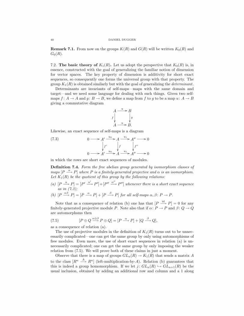
40 DANIEL DUGGER
Remark 7.1. From now on the groups K(R) and G(R) will be written K0(R) andG0(R).
7.2. The basic theory of K1(R). Let us adopt the perspective that K0(R) is, inessence, constructed with the goal of generalizing the familiar notion of dimensionfor vector spaces. The key property of dimension is additivity for short exactsequences, so consequently one forms the universal group with that property. ThegroupK1(R) is obtained similarly but with the goal of generalizing the determinant .
Determinants are invariants of self-maps—maps with the same domain andtarget—and we need some language for dealing with such things. Given two self-maps f : A→ A and g : B → B, we define a map from f to g to be a map u : A→ Bgiving a commutative diagram
Au //
f
B
g
A
u // B.
Likewise, an exact sequence of self-maps is a diagram
0 // A′u0 //
f ′
Au1 //
f
A′′ //
f ′′
0
0 // A′u0 // A
u1 // A′′ // 0
(7.3)
in which the rows are short exact sequences of modules.
Definition 7.4. Form the free abelian group generated by isomorphism classes ofmaps [P α−→ P ] where P is a finitely-generated projective and α is an isomorphism.Let K1(R) be the quotient of this group by the following relations:
(a) [P α−→ P ] = [P ′ α′−→ P ′]+[P ′′ α′′−→ P ′′] whenever there is a short exact sequenceas in (7.3);
(b) [Pαβ−→ P ] = [P α−→ P ] + [P
β−→ P ] for all self-maps α, β : P → P .
Note that as a consequence of relation (b) one has that [P id−→ P ] = 0 for anyfinitely-generated projective module P . Note also that if α : P → P and β : Q→ Qare automorphsms then
[P ⊕Q α⊕β−→ P ⊕Q] = [P α−→ P ] + [Qβ−→ Q],(7.5)
as a consequence of relation (a).The use of projective modules in the definition of K1(R) turns out to be unnec-
essarily complicated—one can get the same group by only using automorphisms offree modules. Even more, the use of short exact sequences in relation (a) is un-necessarily complicated; one can get the same group by only imposing the weakerrelation from (7.5). We will prove both of these claims in just a moment.
Observe that there is a map of groups GLn(R)→ K1(R) that sends a matrix Ato the class [Rn A−→ Rn] (left-multiplication-by-A). Relation (b) guarantees thatthis is indeed a group homomorphism. If we let j : GLn(R) → GLn+1(R) be theusual inclusion, obtained by adding an additional row and column and a 1 along
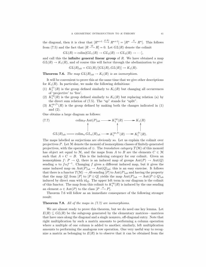
A GEOMETRIC INTRODUCTION TO K-THEORY 41
the diagonal, then it is clear that [Rn+1 j(A)−→ Rn+1] = [Rn A−→ Rn]. This followsfrom (7.5) and the fact that [R id−→ R] = 0. Let GL(R) denote the colimit
GL(R) = colim[GL1(R)→ GL2(R)→ GL3(R)→ · · · ],and call this the infinite general linear group of R. We have obtained a mapGL(R)→ K1(R), and of course this will factor through the abelianization to give
GL(R)ab = GL(R)/[GL(R), GL(R)]→ K1(R).
Theorem 7.6. The map GL(R)ab → K1(R) is an isomorphism.
It will be convenient to prove this at the same time that we give other descriptionsfor K1(R). In particular, we make the following definitions:
(1) Kfr1 (R) is the group defined similarly to K1(R) but changing all occurrences
of ‘projective’ to ‘free’.(2) Ksp
1 (R) is the group defined similarly to K1(R) but replacing relation (a) bythe direct sum relation of (7.5). The “sp” stands for “split”.
(3) Ksp,fr1 (R) is the group defined by making both the changes indicated in (1)
and (2).One obtains a large diagram as follows:
colimP Aut(P )ab // // Ksp1 (R) // // K1(R)
GL(R)ab colimnGLn(R)ab // //
OO
Ksp,fr1 (R) // //
OO
Kfr1 (R).
OO(7.7)
The maps labelled as surjections are obviously so. Let us explain the colimit overprojectives P . Let M denote the monoid of isomorphism classes of finitely-generatedprojectives, with the operation of ⊕. The translation category T (M) of this monoidhas object set equal to M, and the maps from A to B are the elements C ∈ M
such that A + C = B. This is the indexing category for our colimit. Given anisomorphism f : P → Q, there is an induced map of groups Aut(P ) → Aut(Q)sending α to fαf−1. Changing f gives a different induced map, but it gives thesame induced map on Aut(P )ab → Aut(Q)ab; this is an easy exercise. It followsthat there is a functor T (M)→ Ab sending [P ] to Aut(P )ab and having the propertythat the map [Q] from [P ] to [P ⊕ Q] yields the map Aut(P )ab → Aut(P ⊕ Q)abinduced by direct sum with idQ. The upper left term in our diagram is the colimitof this functor. The map from this colimit to Ksp
1 (R) is induced by the one sendingan element α ∈ Aut(P ) to the class [P α−→ P ].
Theorem 7.6 will follow as an immediate consequence of the following strongerresult:
Theorem 7.8. All of the maps in (7.7) are isomorphisms.
We are almost ready to prove this theorem, but we do need one key lemma. LetE(R) ⊆ GL(R) be the subgroup generated by the elementary matrices—matricesthat have ones along the diagonal and a single nonzero, off-diagonal entry. Note thatright multiplication by such a matrix amounts to performing a column operationwhere a multiple of one column is added to another; similarly, left multiplicationamounts to performing the analogous row operation. One very useful way to recog-nize a matrix as belonging to E(R) is to observe that it can be obtained from the

42 DANIEL DUGGER
identity matrix by using these types of row and column operations. It is useful tosay that a column or row operation is allowable if the corresponding elementarymatrix belongs to E(R).
Lemma 7.9.(a) For any X ∈Mn(R) the matrix
[I X0 I
]and its transpose belong to E(R).
(b) If A ∈ GLn(R) then[A 00 A−1
]∈ E(R).
(c) Let A be a matrix obtained from the identity by switching two colums and mul-tiplying one of the switched columns by −1. Then A ∈ E(R), and similarly forthe transpose of A.
Proof. For part (a) just note that[I X0 I
]can be obtained from the identity matrix
by a sequence of allowable column operations of the type discussed above. For thetranspose, use row operations.
For (b) consider the following chain of matrices:[I 00 I
]∼[I A0 I
]∼[
I AA−2 −A−1 A−1
]∼[
A 0A−2 −A−1 A−1
]∼[A 00 A−1
].
Passage from each matrix to the next can be done by allowable row and columnoperations; alternatively, each matrix can be obtained from its predecessor by leftor right multiplication by a matrix of the type considered in (a).
Finally, for (c) we argue directly in terms of column operations. If v and w aretwo columns consider the following chain
v, w 7→ v, w − v 7→ w,w − v 7→ w,−v.Each link involves adding a multiple of one column to another, and is thereforeallowable; therefore the composite operation is allowable.
The following is the key lemma that we will need in our proof of Theorem 7.8:
Lemma 7.10 (Whitehead Lemma). E(R) = [GL(R), GL(R)]
Proof. For the ⊆ direction we consider three columns u, v, w, and the followingchain of operations (where r, s ∈ R):
u, v, w 7→ u, v + ru, w 7→ u, v + ru, w + sv + sru 7→ u, v, w + sv + sru
7→ u, v, w + sru.
It should be clear what column operation is being used in each step. Note that thethird and fourth operations are the inverses of the first and second, so the compositeit a commutator. This shows that any column operation of the type “add a multipleof one column to another” is a commutator, and therefore E(R) ⊆ [GL(R), GL(R)].(We have actually shown En(R) ⊆ [GLn(R), GLn(R)] for n ≥ 3).
For the other subset, let A,B ∈ GLn(R). Consider the following identity:[ABA−1B−1 0
0 I
]·[B 00 B−1
]·[A 00 A−1
]=[AB 00 B−1A−1
].
The first matrix is identified with the commutator of A and B inside GL(R), and allof the other matrices are in E(R) by Lemma 7.9(b). So [A,B] ∈ E(R) as well.
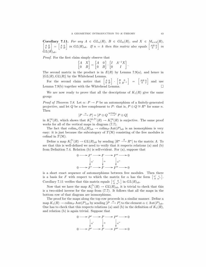
A GEOMETRIC INTRODUCTION TO K-THEORY 43
Corollary 7.11. For any A ∈ GLn(R), B ∈ GLk(R), and X ∈ Mn×k(R),[A X0 B
]=[A 00 B
]in GL(R)ab. If n = k then this matrix also equals
[AB 00 I
]in
GL(R)ab.
Proof. For the first claim simply observe that[A X0 B
]=[A 00 B
]·[I A−1X0 I
].
The second matrix in the product is in E(R) by Lemma 7.9(a), and hence in[GL(R), GL(R)] by the Whitehead Lemma.
For the second claim notice that[A 00 B
]·[B 00 B−1
]=
[AB 00 I
]and use
Lemma 7.9(b) together with the Whitehead Lemma.
We are now ready to prove that all the descriptions of K1(R) give the samegroup:
Proof of Theorem 7.8. Let α : P → P be an automorphism of a finitely-generatedprojective, and let Q be a free complement to P : that is, P ⊕Q ∼= Rn for some n.Then
[P α−→ P ] = [P ⊕Q α⊕idQ−→ P ⊕Q]
in Ksp1 (R), which shows that Ksp,fr
1 (R) → Ksp1 (R) is surjective. The same proof
works for all of the vertical maps in diagram (7.7).The fact that colimnGLn(R)ab → colimP Aut(P )ab is an isomorphism is very
easy: it is just because the subcategory of T (M) consisting of the free modules iscofinal in T (M).
Define a map Kfr1 (R)→ GL(R)ab by sending [Rn A−→ Rn] to the matrix A. To
see that this is well-defined we need to verify that it respects relations (a) and (b)from Definition 7.4. Relation (b) is self-evident. For (a), suppose that
0 // F ′ //
α′
F //
α
F ′′ //
α′′
0
0 // F ′ // F // F ′′ // 0
is a short exact sequence of automorphisms between free modules. Then thereis a basis for F with respect to which the matrix for α has the form
[α′ ∗0 α′′
].
Corollary 7.11 verifies that this matrix equals[α′ 00 α′′
]in GL(R)ab.
Now that we have the map Kfr1 (R) → GL(R)ab, it is trivial to check that this
is a two-sided inverse for the map from (7.7). It follows that all the maps in thebottom row of that diagram are isomorphisms.
The proof for the maps along the top row proceeds in a similar manner. Define amapK1(R)→ colimP Aut(P )ab by sending [P α−→ P ] to the element α ∈ Aut(P )ab.One has to check that this respects relations (a) and (b) in the definition of K1(R),and relation (b) is again trivial. Suppose that
0 // P ′ //
α′
P //
α
P ′′ //
α′′
0
0 // P ′ // P // P ′′ // 0
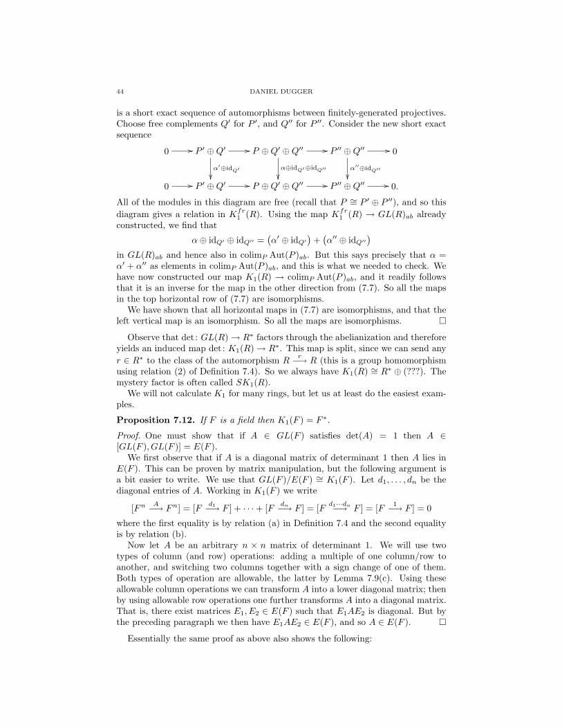
44 DANIEL DUGGER
is a short exact sequence of automorphisms between finitely-generated projectives.Choose free complements Q′ for P ′, and Q′′ for P ′′. Consider the new short exactsequence
0 // P ′ ⊕Q′ //
α′⊕idQ′
P ⊕Q′ ⊕Q′′ //
α⊕idQ′⊕idQ′′
P ′′ ⊕Q′′ //
α′′⊕idQ′′
0
0 // P ′ ⊕Q′ // P ⊕Q′ ⊕Q′′ // P ′′ ⊕Q′′ // 0.
All of the modules in this diagram are free (recall that P ∼= P ′ ⊕ P ′′), and so thisdiagram gives a relation in Kfr
1 (R). Using the map Kfr1 (R) → GL(R)ab already
constructed, we find that
α⊕ idQ′ ⊕ idQ′′ =(α′ ⊕ idQ′
)+(α′′ ⊕ idQ′′
)in GL(R)ab and hence also in colimP Aut(P )ab. But this says precisely that α =α′ + α′′ as elements in colimP Aut(P )ab, and this is what we needed to check. Wehave now constructed our map K1(R) → colimP Aut(P )ab, and it readily followsthat it is an inverse for the map in the other direction from (7.7). So all the mapsin the top horizontal row of (7.7) are isomorphisms.
We have shown that all horizontal maps in (7.7) are isomorphisms, and that theleft vertical map is an isomorphism. So all the maps are isomorphisms.
Observe that det : GL(R)→ R∗ factors through the abelianization and thereforeyields an induced map det : K1(R)→ R∗. This map is split, since we can send anyr ∈ R∗ to the class of the automorphism R
r−→ R (this is a group homomorphismusing relation (2) of Definition 7.4). So we always have K1(R) ∼= R∗ ⊕ (???). Themystery factor is often called SK1(R).
We will not calculate K1 for many rings, but let us at least do the easiest exam-ples.
Proposition 7.12. If F is a field then K1(F ) = F ∗.
Proof. One must show that if A ∈ GL(F ) satisfies det(A) = 1 then A ∈[GL(F ), GL(F )] = E(F ).
We first observe that if A is a diagonal matrix of determinant 1 then A lies inE(F ). This can be proven by matrix manipulation, but the following argument isa bit easier to write. We use that GL(F )/E(F ) ∼= K1(F ). Let d1, . . . , dn be thediagonal entries of A. Working in K1(F ) we write
[Fn A−→ Fn] = [F d1−→ F ] + · · ·+ [F dn−→ F ] = [F d1···dn−→ F ] = [F 1−→ F ] = 0
where the first equality is by relation (a) in Definition 7.4 and the second equalityis by relation (b).
Now let A be an arbitrary n × n matrix of determinant 1. We will use twotypes of column (and row) operations: adding a multiple of one column/row toanother, and switching two columns together with a sign change of one of them.Both types of operation are allowable, the latter by Lemma 7.9(c). Using theseallowable column operations we can transform A into a lower diagonal matrix; thenby using allowable row operations one further transforms A into a diagonal matrix.That is, there exist matrices E1, E2 ∈ E(F ) such that E1AE2 is diagonal. But bythe preceding paragraph we then have E1AE2 ∈ E(F ), and so A ∈ E(F ).
Essentially the same proof as above also shows the following:

A GEOMETRIC INTRODUCTION TO K-THEORY 45
Proposition 7.13. Let R be a Euclidean domain. Then det : K1(R) → R∗ isan isomorphism. In particular, K1(Z) = 1,−1 ∼= Z/2 and when F is a fieldK1(F [t]) ∼= F ∗.
Proof. We must again show that if A ∈ GLn(R) has det(A) = 1 then A ∈ E(R).For any fixed row of A, the ideal generated by the elements in that row containsdet(A) and is therefore the unit ideal. Pick an element x of smallest degree inthis row and then use column operations (and the Euclidean division property) toarrange all other elements in this row to be either zero or have degree smaller thanx. By repeating this process, eventually the row will contain a unit. Do a signedtransposition to switch this unit into position (1, 1), and then do row operations toclear out all other terms in the first column. Repeat this process for the submatrixobtained by deleting the first row and column, and so forth. Eventually the matrixwill be reduced to a diagonal matrix, necessarily of determinant 1. Such a diagonalmatrix lies in E(R), so this proves A also lies in E(R).
7.14. Longer localization sequences.
Proposition 7.15. There is a unique map ∂ : K1(S−1R) → K0(R,S) having theproperty that if α : Rn → Rn is such that S−1α is an isomorphism, then ∂ sends
[S−1RnS−1α−→ S−1Rn] to the class of the chain complex 0 → Rn
α−→ Rn → 0(concentrated in degrees 0 and 1).
Proof. First, assume that β : (S−1R)n → (S−1R)n. Let A be the matrix for β withrespect to the standard basis, and let u ∈ S be an element such that uA has entriesin R (e.g., take u to be the product of all the denominators of the entries in A).Then uA represents a map β′ : Rn → Rn, and we have the commutative diagram
(S−1R)nβ // (S−1R)n
uIn // (S−1R)n
Rn
OO
β′ // Rn
OO
where the vertical maps are localization. This diagram gives uIn β ∼= S−1β′, andso [uIn] + [β] = [S−1β′] in K1(S−1R). Note that [uIn] = n[uI1], and uI1 is itselfthe localization of the multiplication-by-u map on R; so we can write
[β] = [S−1β′]− n[S−1u].(7.16)
This shows that K1(R) is generated by classes [S−1α] for α : Rn → Rn, and wehave thereby proven the uniqueness part of the proposition.
For existence, we will define a map ∂ : Ksp,fr1 (R) → K0(R,S) and then appeal
to Theorem 7.8. Given a map β : (S−1R)n → (S−1R)n, choose a u ∈ S such thatthe standard matrix representing uβ has entries in R. Consider the assignment
β 7→ F (β, u) = [Rnuβ−→ Rn]− n[R u−→ R] ∈ K0(R,S).
Note that this expression doesn’t come out of thin air: the expected homomorphism∂, if it exists, must have this form by (7.16). It remains to show that the aboveformula does indeed define a homomorphism.
We first show that F (β, u) does not depend on the choice of u. It suffices toprove that F (β, tu) = F (β, u) for any t ∈ S; for if u′ is another choice for u then
46 DANIEL DUGGER
we would have F (β, u) = F (β, u′u) = F (β, u′). But now we just compute that
F (β, tu) = [Rntuβ−→ Rn]− n[R tu−→ R]
= [Rn t−→ Rn] + [Rnuβ−→ Rn]− n
[[R t−→ R] + [R u−→ R]
]= [Rn
uβ−→ Rn]− n[R u−→ R]
(the second equality is by Lemma 5.12, applied twice).Let us now write F (β) instead of F (β, u). The last thing that must be checked
is that F (β ⊕ β′) = F (β) + F (β′), but this is obvious. So we have established theexistence of ∂ : K1(R)→ K0(R,S) having the desired properties.
Theorem 7.17 (Localization sequence for K-theory). Let R be a commutative ringand S ⊆ R a multiplicative system. The following sequence is exact:
K1(R) −→ K1(S−1R) ∂−→ K0(R,S) −→ K0(R) −→ K0(S−1R).
Proof. We will not prove exactness at K1(S−1R), as this is a bit difficult and wouldtake us too far afield. Exactness at K0(R) was already proven in Proposition 5.13,so it only remains to verify exactness at K0(R,S).
Let x ∈ K0(R,S). We know by Theorem 5.14 that x can be written in theform x = [P1 → P0] − [Q1 → Q0] for finitely-generated projectives P0, P1, Q0, Q1
over R and maps α : P1 → P0, β : Q1 → Q0 that become isomorphisms afterS-localization. Consider the isomorphism S−1Q0 → S−1Q1 that is the inverseto S−1β. By Lemma 4.7(b) there is a map γ : Q0 → Q1 whose localization isisomorphic to this map. Notice that
x = [P1 → P0] + [Q0 → Q1]−([Q0 → Q1] + [Q1 → Q0]
)= [P1 ⊕Q0 → P0 ⊕Q1]− [Q0 ⊕Q1 → Q1 ⊕Q0].
So by replacing our original P ’s and Q’s we can assume that Q0 = Q1.Let G be a projective such that Q0 ⊕G is free, and observe that
x = x− [G id−→ G] = [P1 → P0]− [Q0 ⊕G→ Q0 ⊕G].
So again, by replacing our chosen Q0 = Q1 we can actually assume that Q0 = Q1
is free. That is, x = [P1α−→ P0]− [Rn
β−→ Rn].Now assume that x maps to zero in K0(R). This just says that [P0] = [P1] in
K0(R), and so there exists a free module G such that P0 ⊕ G ∼= P1 ⊕ G. Sincex = x+ [G id−→ G] we see that we can write x as
x = [Rk α−→ Rk]− [Rnβ−→ Rn]
where α and β become isomorphisms after S-localization. It is now immediate thatx is in the image of ∂; to be completely specific,
x = ∂([S−1Rk
S−1α−→ S−1Rk]− [S−1RnS−1β−→ S−1Rn]
).
Example 7.18. This example will be a “reality check”. We won’t learn anythingnew, but we will see that the localization sequence is doing something sensible.Let R be a discrete valuation ring (a regular local ring whose maximal ideal isprincipal), and let F be the quotient field. Let π be a generator for the maximal
A GEOMETRIC INTRODUCTION TO K-THEORY 47
ideal, and let S = 1, x, x2, . . .. Note that S−1R = F . The localization sequencetakes on the form
K1(R)→ F ∗∂−→ K0(R,S)→ Z
∼=−→ Zwhere we are using K1(F ) ∼= F ∗, K0(R) ∼= Z (because R is a PID), and the mapK0(R)→ K0(F ) ∼= Z sends [R] to [F ] and is therefore an isomorphism.
Although we have not calculated K1(R), the commutative diagram
K1(R) //
det
K1(F )
det ∼=
R∗ // // F ∗
shows that the image of K1(R) in F ∗ is just R∗. Our localization sequence distillsinto a single isomorphism
F ∗/R∗∂−→ K0(R,S).
The group F ∗/R∗ is readily checked to be Z, where the isomorphism Z ∼= F ∗/R∗
sends n to [πn]. On the other hand, we also know by Theorem 5.15 that K0(R,S) ∼=G(M |S−1M = 0). A finitely-generated module M satisfies S−1M = 0 if and onlyif M is killed by a power of x, or equivalently if M has finite length over R. Themap ` : G(M |S−1M = 0)→ Z is easily checked to be an isomorphism.
Finally, let us analyze the map ∂. Given an element a ∈ F ∗, we write a =r/πn for some r ∈ R∗ and n ≥ 0. The description of ∂ given in the proof ofProposition 7.15 shows that
∂(a) = [R r−→ R]− [R πn
−→ R] = [R r−→ R]− n[R π−→ R].
The isomorphism K0(R,S) → G(M |S−1M = 0) sends a complex P• to the alter-nating sum of its homology modules, so under this isomorphism we would write
∂(a) = [R/rR]− n[R/πR].
Note that `(R/πR) = 1. We can write r = uπk for some unit u ∈ R and n ≥ 0, inwhich case R/rR ∼= R/πkR and so `(R/rR) = k. It follows that the composite
F ∗∂−→ K0(R,S)
∼=−→ G(M |S−1M = 0)∼=−→ Z
is just the usual π-adic valuation on F ∗.
The following example generalizes the previous one, but is a bit more interesting.
Example 7.19. Let D be a Dedekind domain—a regular ring of dimension one.In such a ring all nonzero primes are maximal ideals. Let S = D − 0 and letF = S−1D be the quotient field. Our localization sequence looks like
K1(D)→ F ∗ → K0(D,S)→ K0(D)→ Z.Just as in the previous example, the image of K1(D) in F ∗ is just D∗. The mapK0(D) → Z is just the usual rank map, so its kernel is K0(D). So we get a shortexact sequence
0→ F ∗/D∗ ∂−→ K0(D,S)→ K0(D)→ 0.

48 DANIEL DUGGER
We know K0(D,S) ∼= G(M |S−1M = 0). The condition S−1M = 0 just says thatM is a torsion module. Consider the evident map
j :⊕P 6=0
G(D/P )→ G(M |S−1M = 0)
where the direct sum is over all nonzero prime ideals and where the map just forgetsthat a module is defined over D/P and instead regards it as a D-module. This mapis clearly surjective: a torsion D-module M will have a prime filtration in which theprimes appearing are all maximal, and [M ] will be the sum of the corresponding[D/P ]’s by the usual argument (see Theorem 2.15 and its proof).
Note that each D/P is a field, and so G(D/P ) ∼= Z. If M is a torsion D-modulethen MP is a torsion DP -module. Since DP is a discrete valuation ring, this meansthat MP has finite length. Define
χ : G(M |S−1M = 0)→⊕P 6=0
G0(R/P )
by sending [M ] to the tuple of integers `DP(MP ), as P runs over all maximal ideals
of D (the only ones that give nonzero lengths are the ones containing AnnM , andthere are only finitely-many of these since they are precisely the minimal primesof AnnM). It is easy to check that χ j = id; since j was already known to besurjective this means they are inverse isomorphisms. So we can rewrite our shortexact sequence as
0→ F ∗/D∗ ∂−→⊕P 6=0
Z→ K0(D)→ 0.
It will be convenient to write eP for the basis element of the free abelian group inthe middle corresponding to the maximal ideal P . Note that these basis elementscorrespond to the closed points of SpecD, and so we are looking at a group of0-cycles.
It remains to analyze the map ∂. By Proposition 7.15, if r ∈ D − 0 then∂(r) = [D r−→ D] ∈ K0(D,S). Under the isomorphisms described above thiscorresponds to the tuple of integers `DP
(DP /rDP ). This is usually called thedivisor class of r, and written
div(r) =∑
`DP(DP /rDP )eP .
It should be thought of as listing all the zeros of the “function” r, together withtheir orders of vanishing (see below for an example). For a general element x ∈ F ∗we would just write x = r/s for r, s ∈ D − 0, and then ∂(x) = div(r) − div(s);this gives the zeros and poles of x, with multiplicities.
The quotient of⊕
P 6=0 Z by the classes div(x) is called the divisor class groupof D; it is isomorphic to the ideal class group from algebraic number theory. Ourshort exact sequence shows that K0(D) is also isomorphic to this group.
To demonstrate the geometric intuition behind div(r), consider the caseD = F [t]where F is algebraically closed. If r = p(t) then the maximal ideals containing rare the ones (t − ai) where ai is a root of p(t). If we write r =
∏(t − aj)mj and
we localize at P = (t − ai), then r becomes a unit multiple of (t − ai)mi and thenumber `DP
(DP /rDP ) is precisely mi. So
div(r) =∑i
mi · e(t−ai),
A GEOMETRIC INTRODUCTION TO K-THEORY 49
as expected. Note that the divisor class group is not very interesting in this case:clearly div is surjective, and so the group is zero. We already knew this for anotherreason, because K0(D) = 0 whenever D is a PID.
Remark 7.20. The localization sequence of Theorem 7.17 can be extended furtherto the left, by definining K-groups Kn(R) and Kn(R,S) for all n ≥ 1. This is thesubject of higher algebraic K-theory.

50 DANIEL DUGGER
Part 2. K-theory in topology
Finite-dimensional linear algebra is a subject that mathematicians understandvery well. There aren’t that many isomorphism types of objects (one for eachdimension), and we have a pretty good understanding of the maps between them.Our next goal in these notes is to explore the idea of doing linear algebra locallyover a fixed base space X. To be slightly more precise, our objects of interest willbe maps of spaces E → X where the fibers carry the structure of vector spaces;a map from E → X to E′ → X is a continuous map F : E → E′, commutingwith the maps down to X, such that F is a linear transformation on each fiber. Itturns out that much of linear algebra carries over easily to this enhanced setting.But there are more isomorphism types of objects here, because the topology of Xallows for some twisting in the vector space structure of the fibers. The surpriseis that studying these ‘twisted vector spaces’ over a base space X quickly leads tointeresting homotopy invariants of X! Topological K-theory is a cohomology theoryfor topological spaces that arises out of this study of fibrewise linear algebra.
8. Vector bundles
A (real) vector space is a set V together with operations +: V × V → V and· : R×V → V satisfying a familiar (but long) list of properties. If X is a topologicalspace, a family of vector spaces over X will be a continuous map p : E → Xtogether with extra data making each fiber p−1(x) into a vector space, with theoperations varying in a continuous manner. The easiest way to say this is as follows:
Definition 8.1. A family of (real) vector spaces is a map p : E → X togetherwith operations +: E ×X E → E and · : R× E → E making the two diagrams
E ×X E
$$HHHH
HHHH
H+ // E
~~~~
~~~
R× E · //
##FFFFFFFF E
~~~~
~~~
X X
commute, and such that the operations make each fiber p−1(x) into a real vectorspace over X.
One could write down the above definition completely category-theoretically, interms of maps and commutative diagrams. Essentially one is defining a “vectorspace object” in the category of spaces over X.
The space X is called the base of the family. If x ∈ X we will usually writeEx for the fiber p−1(x) regarded with its vector space structure. The dimension ofEx is called the rank of the family at x, and denoted rankx(E). The rank of E isdefined to be
rank(E) = suprankx(E) |x ∈ X,where we include the possibility rank(E) =∞ (although we will never need this).
We leave it to the reader to define a map between families of vector spaces, anisomorphism between families of vector spaces, a “subspace” of a family of vectorspaces, and so on. All of the definitions from linear algebra can easily be adapted.
A GEOMETRIC INTRODUCTION TO K-THEORY 51
Example 8.2.(a) The simplest example is E = X × Rn, with the projection map X × Rn → X.
This is called the trivial family of rank n, and it is often denoted simply byn (with the space X understood).
(b) Let E = (x, v) |x ∈ R2, v ∈ R.〈x〉, and let p : E → R2 be projection onto thefirst coordinate. Define (x, v) + (x, v′) = (x, v + v′) and r.(x, v) = (x, rv). Thismakes E → R2 into a family of vector spaces. Note that the fiber p−1(x) isone-dimensional for x 6= 0, but 0-dimensional when x = 0.
(c) Let X = R. Let e1, e2 be the standard basis for R2. Let E ⊆ X × R2 be theunion of (x, re1) |x ∈ Q, r ∈ R and (x, re2) |x ∈ X\Q, r ∈ R. Recall from(a) that X × R2 → X is a family of vector spaces, and note that E becomes asub-family of vector spaces under the same operations.
The family of vector spaces from Example 8.2(c) perhaps makes it clear that thisnotion is too wild to be of much use: there are too many ‘crazy’ families of vectorspaces like this one. One fixes this by adding a condition that forces the fibers tovary continuously, in a certain sense. This is done as follows:
Definition 8.3. A vector bundle is a family of vector spaces p : E → X suchthat for each x ∈ X there is a neighborhood x ∈ U ⊆ X, an n ∈ Z≥0, and anisomorphism of families of vector spaces
p−1(U)
##FFFFFFFF
∼= // U × Rn
wwww
wwww
w
U
Usually one simply says that a vector bundle is a family of vector spaces that islocally trivial. The isomorphism in the above diagram is called a “local trivializa-tion”.
Remark 8.4. Note that the n appearing in Definition 8.3 depends on the point x.It is called the rank of the vector bundle at x, and denoted rankx(E). It is easy toprove that the rank is constant on the connected components of X. Vector bundlesof rank 1 are often called line bundles, and bundles of rank 2 are called planebundles.
Notation 8.5. If p : E → X is a family of vector spaces and A → X is a subspace,then p−1(A) → A is also a family of vector spaces. We will usually write thisrestriction as E|A. Note that if E is a vector bundle then so is E|A, by a simpleargument. The construction E|A is a special case of a pullback bundle, which wewill discuss in Section 8.9.
Of the families of vector spaces we considered in Example 8.2, only the trivialfamily from (a) is a vector bundle. Before discussing more interesting examples, itwill be useful to have a mechanism for deciding when a family of vector spaces istrivial. If p : E → X is a family of vector spaces, a section of p is a map s : X → Esuch that ps = id. The set of sections is denoted Γ(E), and this becomes a vectorspace using pointwise addition and multiplication in the fibers of E. A collectionof sections s1, . . . , sr is linearly independent if the vectors s1(x), s2(x), . . . , sr(x)are linearly independent in Ex for every x ∈ X.
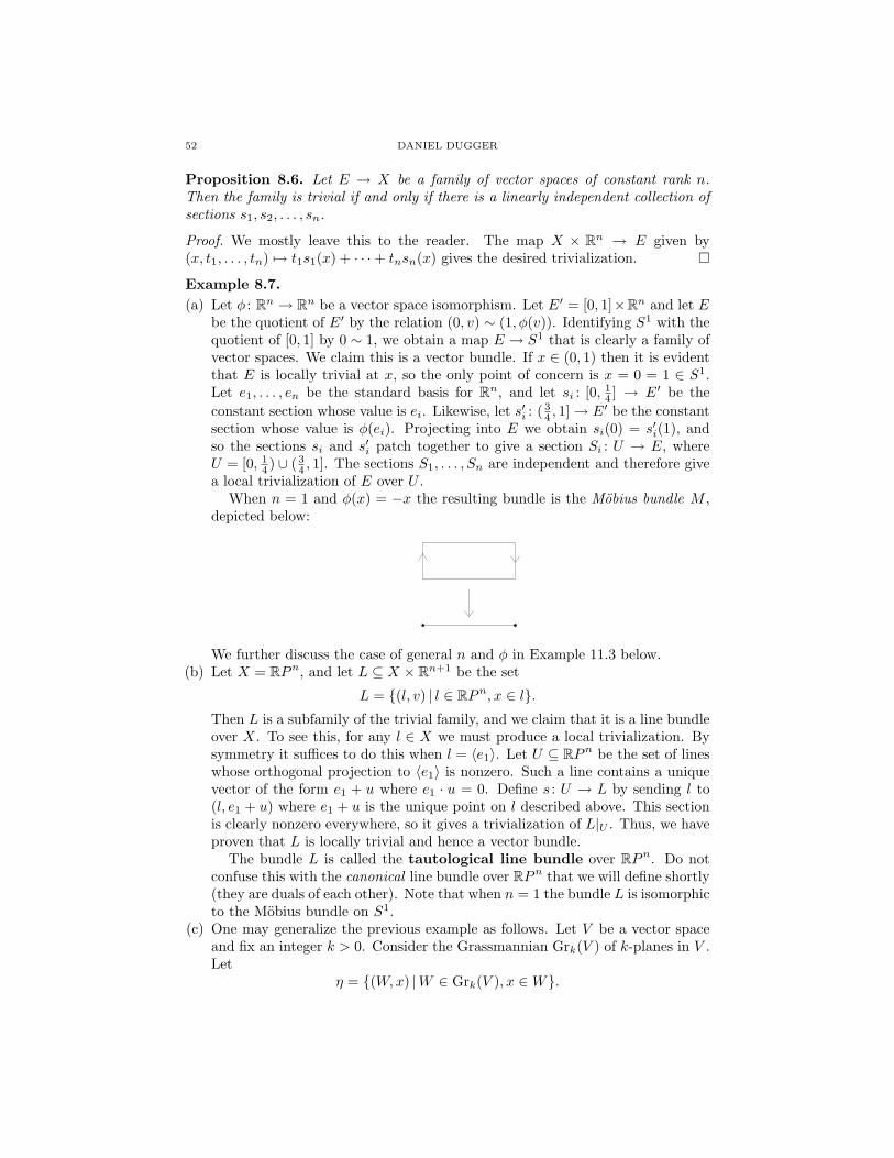
52 DANIEL DUGGER
Proposition 8.6. Let E → X be a family of vector spaces of constant rank n.Then the family is trivial if and only if there is a linearly independent collection ofsections s1, s2, . . . , sn.
Proof. We mostly leave this to the reader. The map X × Rn → E given by(x, t1, . . . , tn) 7→ t1s1(x) + · · ·+ tnsn(x) gives the desired trivialization.
Example 8.7.(a) Let φ : Rn → Rn be a vector space isomorphism. Let E′ = [0, 1]×Rn and let E
be the quotient of E′ by the relation (0, v) ∼ (1, φ(v)). Identifying S1 with thequotient of [0, 1] by 0 ∼ 1, we obtain a map E → S1 that is clearly a family ofvector spaces. We claim this is a vector bundle. If x ∈ (0, 1) then it is evidentthat E is locally trivial at x, so the only point of concern is x = 0 = 1 ∈ S1.Let e1, . . . , en be the standard basis for Rn, and let si : [0, 1
4 ] → E′ be theconstant section whose value is ei. Likewise, let s′i : ( 3
4 , 1]→ E′ be the constantsection whose value is φ(ei). Projecting into E we obtain si(0) = s′i(1), andso the sections si and s′i patch together to give a section Si : U → E, whereU = [0, 1
4 ) ∪ ( 34 , 1]. The sections S1, . . . , Sn are independent and therefore give
a local trivialization of E over U .When n = 1 and φ(x) = −x the resulting bundle is the Mobius bundle M ,
depicted below:
We further discuss the case of general n and φ in Example 11.3 below.(b) Let X = RPn, and let L ⊆ X × Rn+1 be the set
L = (l, v) | l ∈ RPn, x ∈ l.Then L is a subfamily of the trivial family, and we claim that it is a line bundleover X. To see this, for any l ∈ X we must produce a local trivialization. Bysymmetry it suffices to do this when l = 〈e1〉. Let U ⊆ RPn be the set of lineswhose orthogonal projection to 〈e1〉 is nonzero. Such a line contains a uniquevector of the form e1 + u where e1 · u = 0. Define s : U → L by sending l to(l, e1 + u) where e1 + u is the unique point on l described above. This sectionis clearly nonzero everywhere, so it gives a trivialization of L|U . Thus, we haveproven that L is locally trivial and hence a vector bundle.
The bundle L is called the tautological line bundle over RPn. Do notconfuse this with the canonical line bundle over RPn that we will define shortly(they are duals of each other). Note that when n = 1 the bundle L is isomorphicto the Mobius bundle on S1.
(c) One may generalize the previous example as follows. Let V be a vector spaceand fix an integer k > 0. Consider the Grassmannian Grk(V ) of k-planes in V .Let
η = (W,x) |W ∈ Grk(V ), x ∈W.

A GEOMETRIC INTRODUCTION TO K-THEORY 53
Projection to the first coordinate π : η → Grk(V ) makes η into a rank k vectorbundle, called the tautological bundle over Grk(V ). To see that it is indeeda bundle, let W ∈ Grk(V ) be an arbitrary k-plane. By choosing an appropriatebasis for V we can just assume W = 〈e1, . . . , ek〉. Equip V with the standarddot product with respect to the e-basis, and let U ⊆ Grk(V ) be the collectionof all k-planes whose orthogonal projection onto W is surjective (equivalently,an isomorphism). One readily checks that this is an open set of W . For eachJ ∈ U let s1(J), . . . , sk(J) be the unique vectors in J that orthogonally projectonto e1, . . . , ek. One checks that these are continuous sections of η|U , and ofcourse they are clearly independent and hence give a local trivialization.
(d) Let M be a smooth manifold, and let TM →M be its tangent bundle. So thefiber over each x ∈ M is the tangent space at x. Let x ∈ M and let U be alocal coordinate patch about x. Let x1, . . . , xn be local coordinate in U , andlet ∂1, . . . , ∂n be the associated vector fields (giving the tangent vectors to thecoordinate curves in this system). Then ∂1, . . . , ∂n are independent sections ofTM , and hence give a local trivialization.
Definition 8.8. A map of vector bundles is just a map of the underlying familiesof vector spaces.
Note that if f : E → F is a map of vector bundles over X then neither ker f norcoker f will necessarily be a vector bundle. For an example, let X = [−1, 1] andlet E = 1. Define f : E → E by letting it be multiplication-by-t on the fiber overt ∈ X.
8.9. Pullback of vector bundles. Suppose that p : E → X is a family of vectorspaces and f : Y → X is a map. One may form the pullback Y ×X E, morecommonly denoted f∗E in bundle theory:
f∗E Y ×X E //
E
Y // X.
A point in f∗E is a pair (y, e) such that f(y) = p(e), and one defines addition andscalar multiplication on f∗E by (y, e) + (y, e′) = (y, e + e′) and r · (y, e) = (y, re).This makes f∗ → Y into a family of vector spaces, called the pullback family.If y ∈ Y then there is an evident map of vector spaces (f∗E)y → Ef(y) which onereadily checks is an isomorphism.
It is easy to see that if E is a vector bundle then so is f∗E; in this case f∗E iscalled the pullback bundle.
Example 8.10.(a) If f is an inclusion Y → X then f∗E is just the restriction E|Y that we have
discussed before.(b) Pullback bundles can be slightly non-intuitive. Let M → S1 be the Mobius
bundle, and let f : S1 → S1 be the map z 7→ z2. We claim that f∗M ∼= 1. Thisis easiest to see if one uses the following model for M :
M =(eiθ, rei
θ2) ∣∣∣ θ ∈ [0, 2π], r ∈ R
.
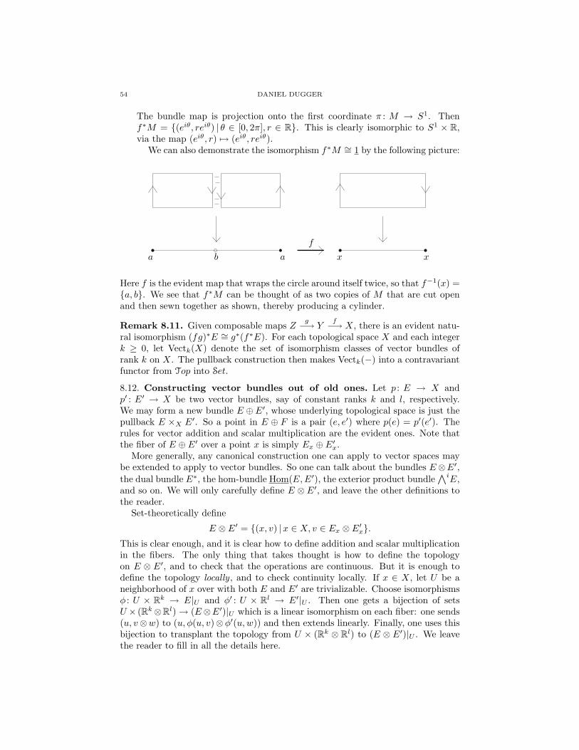
54 DANIEL DUGGER
The bundle map is projection onto the first coordinate π : M → S1. Thenf∗M = (eiθ, reiθ) | θ ∈ [0, 2π], r ∈ R. This is clearly isomorphic to S1 × R,via the map (eiθ, r) 7→ (eiθ, reiθ).
We can also demonstrate the isomorphism f∗M ∼= 1 by the following picture:
xxa b a
f
Here f is the evident map that wraps the circle around itself twice, so that f−1(x) =a, b. We see that f∗M can be thought of as two copies of M that are cut openand then sewn together as shown, thereby producing a cylinder.
Remark 8.11. Given composable maps Zg−→ Y
f−→ X, there is an evident natu-ral isomorphism (fg)∗E ∼= g∗(f∗E). For each topological space X and each integerk ≥ 0, let Vectk(X) denote the set of isomorphism classes of vector bundles ofrank k on X. The pullback construction then makes Vectk(−) into a contravariantfunctor from Top into Set.
8.12. Constructing vector bundles out of old ones. Let p : E → X andp′ : E′ → X be two vector bundles, say of constant ranks k and l, respectively.We may form a new bundle E ⊕E′, whose underlying topological space is just thepullback E ×X E′. So a point in E ⊕ F is a pair (e, e′) where p(e) = p′(e′). Therules for vector addition and scalar multiplication are the evident ones. Note thatthe fiber of E ⊕ E′ over a point x is simply Ex ⊕ E′x.
More generally, any canonical construction one can apply to vector spaces maybe extended to apply to vector bundles. So one can talk about the bundles E⊗E′,the dual bundle E∗, the hom-bundle Hom(E,E′), the exterior product bundle /\iE,and so on. We will only carefully define E ⊗ E′, and leave the other definitions tothe reader.
Set-theoretically define
E ⊗ E′ = (x, v) |x ∈ X, v ∈ Ex ⊗ E′x.This is clear enough, and it is clear how to define addition and scalar multiplicationin the fibers. The only thing that takes thought is how to define the topologyon E ⊗ E′, and to check that the operations are continuous. But it is enough todefine the topology locally , and to check continuity locally. If x ∈ X, let U be aneighborhood of x over with both E and E′ are trivializable. Choose isomorphismsφ : U × Rk → E|U and φ′ : U × Rl → E′|U . Then one gets a bijection of setsU × (Rk⊗Rl)→ (E⊗E′)|U which is a linear isomorphism on each fiber: one sends(u, v⊗w) to (u, φ(u, v)⊗φ′(u,w)) and then extends linearly. Finally, one uses thisbijection to transplant the topology from U × (Rk ⊗ Rl) to (E ⊗ E′)|U . We leavethe reader to fill in all the details here.
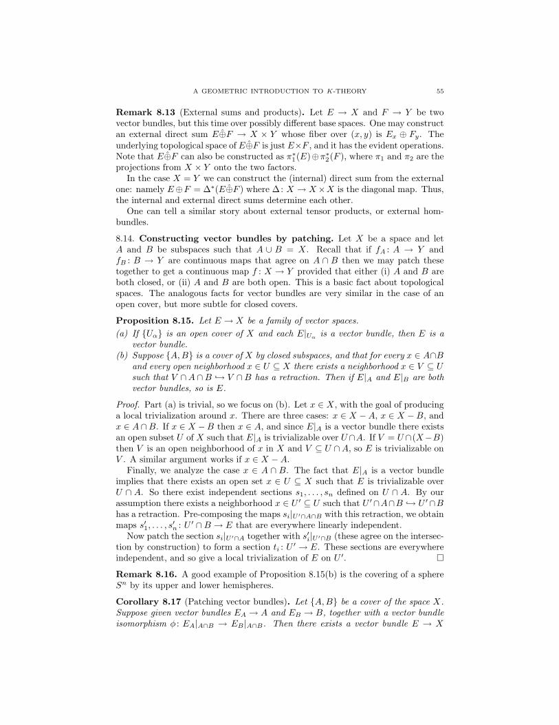
A GEOMETRIC INTRODUCTION TO K-THEORY 55
Remark 8.13 (External sums and products). Let E → X and F → Y be twovector bundles, but this time over possibly different base spaces. One may constructan external direct sum E⊕F → X × Y whose fiber over (x, y) is Ex ⊕ Fy. Theunderlying topological space of E⊕F is just E×F , and it has the evident operations.Note that E⊕F can also be constructed as π∗1(E)⊕π∗2(F ), where π1 and π2 are theprojections from X × Y onto the two factors.
In the case X = Y we can construct the (internal) direct sum from the externalone: namely E⊕F = ∆∗(E⊕F ) where ∆: X → X×X is the diagonal map. Thus,the internal and external direct sums determine each other.
One can tell a similar story about external tensor products, or external hom-bundles.
8.14. Constructing vector bundles by patching. Let X be a space and letA and B be subspaces such that A ∪ B = X. Recall that if fA : A → Y andfB : B → Y are continuous maps that agree on A ∩ B then we may patch thesetogether to get a continuous map f : X → Y provided that either (i) A and B areboth closed, or (ii) A and B are both open. This is a basic fact about topologicalspaces. The analogous facts for vector bundles are very similar in the case of anopen cover, but more subtle for closed covers.
Proposition 8.15. Let E → X be a family of vector spaces.(a) If Uα is an open cover of X and each E|Uα
is a vector bundle, then E is avector bundle.
(b) Suppose A,B is a cover of X by closed subspaces, and that for every x ∈ A∩Band every open neighborhood x ∈ U ⊆ X there exists a neighborhood x ∈ V ⊆ Usuch that V ∩A∩B → V ∩B has a retraction. Then if E|A and E|B are bothvector bundles, so is E.
Proof. Part (a) is trivial, so we focus on (b). Let x ∈ X, with the goal of producinga local trivialization around x. There are three cases: x ∈ X −A, x ∈ X −B, andx ∈ A∩B. If x ∈ X −B then x ∈ A, and since E|A is a vector bundle there existsan open subset U of X such that E|A is trivializable over U ∩A. If V = U ∩(X−B)then V is an open neighborhood of x in X and V ⊆ U ∩A, so E is trivializable onV . A similar argument works if x ∈ X −A.
Finally, we analyze the case x ∈ A ∩ B. The fact that E|A is a vector bundleimplies that there exists an open set x ∈ U ⊆ X such that E is trivializable overU ∩ A. So there exist independent sections s1, . . . , sn defined on U ∩ A. By ourassumption there exists a neighborhood x ∈ U ′ ⊆ U such that U ′∩A∩B → U ′∩Bhas a retraction. Pre-composing the maps si|U ′∩A∩B with this retraction, we obtainmaps s′1, . . . , s
′n : U ′ ∩B → E that are everywhere linearly independent.
Now patch the section si|U ′∩A together with s′i|U ′∩B (these agree on the intersec-tion by construction) to form a section ti : U ′ → E. These sections are everywhereindependent, and so give a local trivialization of E on U ′.
Remark 8.16. A good example of Proposition 8.15(b) is the covering of a sphereSn by its upper and lower hemispheres.
Corollary 8.17 (Patching vector bundles). Let A,B be a cover of the space X.Suppose given vector bundles EA → A and EB → B, together with a vector bundleisomorphism φ : EA|A∩B → EB |A∩B. Then there exists a vector bundle E → X
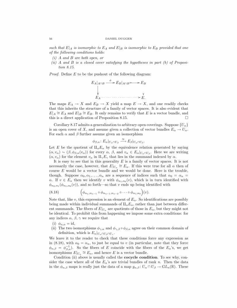
56 DANIEL DUGGER
such that E|A is isomorphic to EA and E|B is isomorphic to EB provided that oneof the following conditions holds:
(i) A and B are both open, or(ii) A and B is a closed cover satisfying the hypotheses in part (b) of Proposi-
tion 8.15.
Proof. Define E to be the pushout of the following diagram:
EA|A∩B
φ // EB |A∩B // // EB
EA // E.
The maps EA → X and EB → X yield a map E → X, and one readily checksthat this inherits the structure of a family of vector spaces. It is also evident thatE|A ∼= EA and E|B ∼= EB . It only remains to verify that E is a vector bundle, andthis is a direct application of Proposition 8.15.
Corollary 8.17 admits a generalization to arbitrary open coverings. Suppose Uαis an open cover of X, and assume given a collection of vector bundles Eα → Uα.For each α and β further assume given an isomorphism
φβ,α : Eα|Uα∩Uβ
∼=−→ Eβ |Uα∩Uβ.
Let E be the quotient of qαEα by the equivalence relation generated by saying(α, vα) ∼ (β, φβ,α(vα)) for every α, β, and vα ∈ Eα|Uα∩Uβ
. Here we are writing(α, vα) for the element vα in qγEγ that lies in the summand indexed by α.
It is easy to see that in this generality E is a family of vector spaces. It is notnecessarily the case, however, that E|Uα
∼= Eα. If this were true for all α then ofcourse E would be a vector bundle and we would be done. Here is the trouble,though. Suppose α0, α1, . . . , αn are a sequence of indices such that α0 = αn =α. If v ∈ Eα then we identify v with φα1,α0(v), which is in turn identified withφα2,α1(φα1,α0(v)), and so forth—so that v ends up being identified with(
φαn,αn−1 φαn−1,αn−2 · · · φα1,α0
)(v).(8.18)
Note that, like v, this expression is an element of Eα. So identifications are possiblybeing made within individual summands of qαEα, rather than just between differ-ent summands. The fibers of E|Uα are quotients of those in Eα, but they might notbe identical. To prohibit this from happening we impose some extra conditions: forany indices α, β, γ we require that
(i) φα,α = id,(ii) The two isomorphisms φγ,α and φγ,β φβ,α agree on their common domain of
definition, which is Eα|Uα∩Uβ∩Uγ .We leave it to the reader to check that these conditions force any expression asin (8.18), with α0 = αn, to just be equal to v (in particular, note that they forceφα,β = φ−1
β,α). So the fibers of E coincide with the fibers of the Eα’s, we getisomorphisms E|Uα
∼= Eα, and hence E is a vector bundle.Condition (ii) above is usually called the cocycle condition. To see why, con-
sider the case where all of the Eα’s are trivial bundles of rank n. Then the datain the φα,β maps is really just the data of a map gα,β : Uα ∩ Uβ → GLn(R). These
A GEOMETRIC INTRODUCTION TO K-THEORY 57
gα,β maps are called transition functions. Condition (ii) is the requirement thatthe transition functions assemble to give a Cech 1-cocycle with values in the groupGLn(R). Condition (i) is just a normalization condition, so that we are deal-ing with ‘normalized’ Cech 1-cocycles. Elements of the Cech cohomology groupH1(U•;GLn(R)) can be seen to be in bijective correspondence with isomorphismclasses of vector bundles on X that are trivializable over the Uα’s; if we take thedirect limit over all open coverings then we obtain a bijection between isomor-phism classes of vector bundles on X and elements of the Cech cohomology groupH1(X;GLn(R)). But we are getting ahead of ourselves here; see Section 11.6 formore discussion.
8.19. Dual bundles. Let E → X be a vector bundle of rank n. Using themethod of Section 8.12 we can define the dual bundle E∗, which set-theoreticallyis (x, v) |x ∈ X, v ∈ E∗x. One can examine this construction in terms of patchingtrivial bundles. Choose an open cover Uα of X with respect to which E is triv-ializable; a choice of trivialization over each Uα then yields a collection of gluingmaps φα,β . We think of E as being built from the trivial bundles Eα = Uα × Rnvia these gluing maps. Then the dual bundle E∗ is built from the trivial bundlesUα × (Rn)∗ via the duals of the gluing maps: that is, (φE
∗)β,α =
(φEα,β
)∗.We will see in a moment (Corollary 8.23) that for real vector bundles over para-
compact Hausdorff spaces one always has E ∼= E∗, although the isomorphism isnot canonical. This is not true for complex or quaternionic bundles, however.
Let L→ CPn be the tautological complex line bundle over CPn. Its (complex)dual L∗ is called the canonical line bundle over CPn. Whereas from a topologicalstandpoint neither L nor L∗ holds a preferential position over the other, in algebraicgeometry there is an important difference between the two. The difference comesfrom the fact that L∗ has certain “naturally defined” sections, whereas L does not.For a point z = [z0 : · · · : zn] ∈ CPn, Lz is the complex line in Cn+1 spannedby (z0, . . . , zn). Given only z ∈ CPn there is no evident way of writing down apoint on Lz, without making some kind of arbitrary choice; said differently, thebundle L does not have any easily-described sections. In contrast, it is much easierto write down a functional on Lz. For example, let φi be the unique functionalon Lz that sends the point (z0, . . . , zn) to zi. Notice that this description dependsonly on z ∈ CPn, not the point (z0, . . . , zn) ∈ Cn+1 that represents it; that is, thefunctional sending (λz0, . . . , λzn) to λzi is the same as φi. In this way we obtainan entire Cn+1’s worth of sections for L∗, by taking linear combinations of the φi’s.
To be clear, it is important to realize that L has plenty of sections—it is just thatone cannot describe them by simple formulas. The slogan to remember is that thebundle L∗ has algebraic sections, whereas L does not. In algebraic geometry thebundle L∗ is usually denoted O(1), whereas L is denoted O(−1). More generally,O(n) denotes (L∗)⊗n when n ≥ 0 (so that O(0) is the trivial line bundle), anddenotes L⊗(−n) when n < 0.
8.20. Inner products on bundles. It is nearly possible to develop everythingwe need from bundle theory without using inner products, and in the rest of thetext we do try to minimize our use of them. But for some results the use of innerproducts does provide significant simplifications of proofs, and so it is good to knowabout them.
58 DANIEL DUGGER
Definition 8.21. Let E → X be a real vector bundle. An inner product on Eis a map of vector bundles E ⊗ E → 1 that induces a positive-definite, symmetric,bilinear form on each fiber Ex. A vector bundle with an inner product is usuallycalled an orthogonal vector bundle.
There is a similar notion for Hermitian inner products on complex vector bun-dles, but here we cannot phrase things in terms of the tensor product because ofconjugate-linearity in one variable. So perhaps the simplest thing is just to say thatif E → X is a complex bundle then a Hermitian inner product is a map E×XE → 1(over X) which induces a Hermitian inner product on each fiber.
Proposition 8.22. Assume that X is paracompact and Hausdorff. Then any realbundle on X admits an inner product, and any complex bundle on X admits aHermitian inner product.
Proof. The idea is to produce the necessary inner products locally, and then use apartition of unity to average the results into a global inner product.
Let E → X be a real vector bundle, and let Uα be an open cover over whichthe bundle is trivial. Choose bundle isomorphisms fα : E|Uα
∼= Uα × Rn, for eachα. Equip Rn with the standard Euclidean inner product, and let 〈−,−〉α be theinner product on E|Uα obtained by transplanting the Euclidean product across theisomorphisms fα.
Let φα be a partition of unity subordinate to the cover Uα. For x ∈ X andv, w ∈ Ex define
〈v, w〉 =∑α
φα(x) · 〈v, w〉α.
It is clear that this is continuous in v and w, bilinear, symmetric, and positive-definite—these follow from the corresponding properties of the forms 〈−,−〉α. Sothis completes the construction.
The proof for Hermitian inner products on a complex bundle is basically identi-cal.
Corollary 8.23. Let E → X be a real vector bundle on a paracompact Hausdorffspace X. Then E is isomorphic to its dual E∗.
Proof. Start by equipping E with an inner product E ⊗ E → 1, and note that thefiberwise forms are nondegenerate (since they are positive-definite). The adjoint ofthe above bundle map is a map E → E∗, and nondegeneracy of the fiberwise formsshows that this is a fiberwise isomorphism.
Remark 8.24. Here is an illuminating exercise. Every complex vector space maybe equipped with a nondegenerate, symmetric bilinear form. Check that the proofof Proposition 8.22 does not generalize to show that every complex vector bundlemay be equipped with a symmetric bilinear form that is nondegenerate on thefibers—in particular, find the point where the proof breaks down. Note that if theproof did generalize, one could show just as in Corollary 8.23 that every complexbundle was isomorphic to its own dual. This is false, as we will see in Example 8.26below. The complex version of Corollary 8.23 says that if E → X is a complexbundle over a paracompact space then E is isomorphic to the conjugate of E∗ (thebundle obtained from E∗ by changing the complex structure so that z ∈ C acts asz).

A GEOMETRIC INTRODUCTION TO K-THEORY 59
Consider a trivial bundle X × Rn → X and equip it with the standard innerproduct. This bundle may be considered as trivial in two different ways: the vectorbundle structure is trivial, and the inner product structure is also trivial. It is notclear a priori that the former property implies the latter, but in fact it does:
Proposition 8.25. Let X be a space. Every inner product on X×Rn is isomorphicto the ‘constant’ inner product provided by the standard Eucliden metric.
Proof. Consider Rn with its standard basis e1, . . . , en. Inner products on Rn are inbijective correspondence with symmetric, positive-definite matrices A ∈Mn×n(R),by sending an inner product 〈−,−〉 to the matrix aij = 〈ei, ej〉. Let Msym,+ denotethe space of such matrices. To give an inner product on the trivial bundle X ×Rnis therefore equivalent to giving a map X →Msym,+.
Given an isomorphism Rn → Rn we may transplant an inner product from thetarget onto the domain; this gives rise to an action of GLn(R) on the space of innerproducts. If P ∈ GLn(R) and A ∈ Msym,+ then the action is P.A = PAPT . Thefact that every inner product on Rn has an orthonormal basis shows that Msym,+
equals the orbit of the identity matrix In under this action. The stabilizer of theidentity is of course the orthogonal group On, and so we obtain the homeomorphismGLn(R)/On ∼= Msym,+.
Now consider the fibration sequence On → GLn(R) → GLn(R)/On. The pro-jection map sends a matrix P to PInP
T = PPT . The inclusion On → GLn(R)is a homotopy equivalence by Gram-Schmidt, and so GLn(R)/On is weakly con-tractible. Standard techniques show that this homogeneous space may be given thestructure of a CW-complex. The lifting diagram
GLn(R)
GLn(R)/On
id //
r77
GLn(R)/On
therefore has a lift as indicated.As we have discussed, our given inner product on X×Rn is represented by a map
X → GLn(R)/On. Compose with r to obtain X → GLn(R). This map specifies abundle isomorphism X×Rn → X×Rn; if we equip the domain with our given innerproduct and the codomain with the standard inner product, this map preserves theinner products and therefore proves the proposition.
Suppose that E → X is a rank n real vector bundle with an inner prod-uct. Choose a trivializing open cover Uα, and for each α fix an inner-product-preserving trivialization fα : E|Uα → Uα × Rn where the codomain has the stan-dard inner product (this is possible by Proposition 8.25). The transition functionsgα,β : Uα ∩ Uβ → GLn(R) therefore factor through On, as they must preserve theinner product. This process is usually referred to as reduction of the structuregroup.
We may use these ideas to give another proof of Corollary 8.23, one that isperhaps more down-to-earth. Let E → X be a real vector bundle on a compactspace, and choose a trivializing cover Uα with respect to which there exist localtrivializations where the transition functions are maps gα,β : Uα ∩Uβ → On. So weobtain E by gluing together the spaces Eα = Uα×Rn via the maps gα,β . But then
60 DANIEL DUGGER
we obtain E∗ by gluing together the spaces Uα × (Rn)∗ via the maps
hβ,α = g∗α,β .
Recall that in terms of matrices the dual is represented by the transpose. Sinceeach gα,β(x) is in On we can write hβ,α(x) = gα,β(x)−1, or
hα,β(x) = hβ,α(x)−1 = gα,β(x).
In other words, the transition functions for E and E∗ are exactly the same, andthat is why the bundles are isomorphic.
We close this section with the promised example of a complex bundle that is notisomorphic to its dual:
Example 8.26. Let D+ and D− denote the upper and lower hemisphere of S2;let S1 be the equator, which we identify with the unit complex numbers. Given amap f : S1 → GLn(C) we may construct a complex bundle on S2 by taking twotrivial bundles nD+
and nD− and gluing them together using the map f : precisely,for z ∈ S1 an element v ∈
(nD+
)z
is glued to f(z) · v ∈(nD−
)z. Here we are using
Corollary 8.17(b). Let E(f) denote the resulting bundle.Observe that giving an isomorphism E(f) → E(g) is equivalent to giving two
maps A : D+ → GLn(R) and B : D− → GLn(C) such that g(z) ·A(z) = B(z) · f(z)for all z ∈ S1. Let us rewrite this as A(z) = g(z)−1B(z)f(z). Now, the mapB|S1 : S1 → GLn(C) is null-homotopic because it extends over D−; so it is (un-based) homotopic to the constant map at 1. Therefore the map z 7→ g(z)−1B(z)f(z)is homotopic to g(z)−1f(z). But A|S1 is also (unbased) homotopic to the constantmap at 1, because it extends over D+. So we have proven that if E(f) ∼= E(g) thenz 7→ g(z)−1f(z) is unbased homotopic to a constant.
Next, observe that the dual of E(f) is E(f ′), where f ′(z) =[f(z)T
]−1. So ifE(f) is isomorphic to its dual then the map z 7→ f(z)T · f(z) is null-homotopic.
Consider the case f(z) = z. Since z 7→ z2 is not null-homotopic, we see thatE(f) is not isomorphic to its dual. The reader may wish to check that E(f) is thetautological line bundle L→ CP 1.
9. Some results from fiberwise linear algebra
Recall that our basic goal is to learn to do linear algebra “over a base space”.The fundamental objects in this setting are the vector bundles, and the maps arethe bundle maps. This section contains a miscellany of results that are frequentlyuseful. This material can be safely skipped the first time through and referred backto as needed.
Lemma 9.1. Let X be any space, and let f : n k be a surjective map of bundles.Then f has a splitting.
Note that the result is not immediately obvious. Of course one can choose asplitting in each fiber, but what guarantees that these can be chosen in a continuousmanner?
Proof. Let W = A ∈ Mk×n | rankA = k, which is the space of surjective mapsRn → Rk (our matrices act on the left). Let Z be the space
Z = (A,B) |A ∈Mk×n, B ∈Mn×k, AB = I,
A GEOMETRIC INTRODUCTION TO K-THEORY 61
which is the space of surjective maps with a chosen splitting. We claim that theprojection map p1 : Z →W is a fiber bundle with fiber Rk(n−k), but defer the prooffor just a moment. The fact that the fiber is contractible then shows that p1 isweak homotopy equivalence.
Consider the diagramZ
∼p1
W W.
The Lie group GLn(R)×GLk(R) acts on W via change-of-basis in the domain andrange, and this action is transitive. So W is homeomorphic to a homogeneous space(GLn(R)×GLk(R))/H for some subgroup H. From this it is not hard to see thatW can be given the structure of a CW-complex. The standard lifting theoremsnow show that there is a lifting r : W → Z in the above diagram.
Our surjective bundle map f : n → k is determined by a map X → W . Com-posing with W → Z, and then projecting to the second coordinate of Z, gives thedesired splitting for f .
It remains to prove the claim about p1 being a fiber bundle. Let A ∈ W . Sincerank(A) = k there is a k×k minor of A that is nonzero; without loss of generality letus assume that it is minor made up of the first k columns of the matrix. Let U ⊆Wbe the subspace consisting of all matrices where this same minor is nonzero, whichis an open neighborhood of A in W . Writing matrices in block form, U consists ofmatrices [X|Y ] where where det(X) 6= 0. Then p−1
1 (U) consists of pairs
αX,Y,J,K =([X Y
],
[JK
])having the property that det(X) 6= 0 and XJ + Y K = Ik. We obtain an iso-morphism U × Mn−k,k(R) ∼= π−1(U) by sending ([X|Y ],K) to αX,Y,J,K withJ = X−1(Ik − Y K).
Note the significance of the map W → Z that is produced in the above proof.This assigns to every surjection Rn → Rk a splitting, and it does so in a continuousmanner. Of course there is no claim that there is a nice formula for how to do this,and in fact there almost certainly is not—but the proof shows that there does existsome way of doing so.
The following proposition is the generalization to arbitrary bundles:
Proposition 9.2. Let X be a paracompact space. Then any surjection of bundlesE F has a splitting.
Proof. Briefly, we choose local splittings and then use a partition of unity to patchthem together.
Choose an open cover Uα such that both E and F are trivializable over eachUα. Lemma 9.1 shows that there are splittings χα : FUα → EUα . Now choose apartition of unity φα subordinate to our open cover. Set χ =
∑α φαχα. This
sum makes sense because the partition of unity is locally finite, and one readilychecks that it is a splitting for f .
The next result gives a useful tool for recognizing vector bundles. The prooffollows the same pattern of the previous two results.
62 DANIEL DUGGER
Proposition 9.3. Let X be any space, and let f : E → F be a map of vectorbundles over X. If f has constant rank then ker f , coker f , and im f are vectorbundles.
Proof. We first prove the result for ker f and coker f . Let x ∈ X, let n = rankx(E),let k = rankx(F ), and let r = rank(f). It will suffice to produce a neighborhood Uof x together with n−r independent sections of ker f over U and k−r independentsections of coker f over U . In particular, this makes it clear that we might as wellassume that E and F are both trivial bundles; in this case f is specified by a mapX →Wr where Wr = A ∈Mk×n | rank(A) = r.
Let Zr be the spaceZr = (A, v1, . . . , vn−r) |A ∈Mk×n, rank(A) = r,
and v1, . . . , vn−r span the kernel of A.One can check that the projection Zr →Wr is a fiber bundle with fiber GLn−r(R),but this is stronger than what we actually need. We only need that the map islocally split: any point in Wr has a neighborhood over which there exists a section.Given a map X →Wr, it will then follow that every point in x has a neighborhoodover which there exists a lifting into Zr, and this will give the n − r independentlocal sections of ker f .
So let A be a point in Wr. Since rank(A) = r, some r× r minor of A is nonzero.Without loss of generality we might as well assume it is the upper left r× r minor.Since rank(A) = r, then for j > r the jth column of A is a linear combination ofthe first r columns in a unique way; said differently, there is a unique vector of theform
vj = ej − s1e1 − s2e2 − · · · − srerthat is in the kernel of A. Here the si’s are certain rational expressions in thematrix entries of A that can be determined using Cramer’s Rule. These formulasdefine sections on the neighborhood U of A consisting of all k× n matrices of rankr whose upper left r × r minor is nonzero. This finishes the proof of our claim.
We have established that ker f is a vector bundle. The proof for coker f is entirelysimilar. Finally, consider the projection F → coker f . This map has constant rank,and so by what has already been established its kernel is a vector bundle. Noticethat this kernel is precisely imα.
The result below is an easy variation on Proposition 9.2; it will be used often,and so it is useful to have it stated explicitly.
Corollary 9.4. Let X be a paracompact space. Then any injection of bundlesE → F has a splitting.
Proof. Let Q be the quotient, which is a vector bundle by Proposition 9.3. ByProposition 9.2 the map F Q has a splitting, which then induces an isomorphismF ∼= E ⊕ Q. The composition F
∼=−→ E ⊕ Q π1−→ E gives the required splitting ofE → F .
The next result is of a somewhat different nature:
Proposition 9.5. Suppose that X is compact and Hausdorff. Then every bundleis a subbundle of some trivial bundle.

A GEOMETRIC INTRODUCTION TO K-THEORY 63
Proof. Let π : E → X be a vector bundle on X. Choose a finite cover U1, . . . , Usover which E is trivializable, which exists because of compactness. For each i choosea trivialization fi : E|Ui
∼=−→ Ui × Rn. Write Fi = π2fi.Let φi be a partition of unity subordinate to the open cover. Define a map
β : E −→ X × Rn × Rn × · · · × Rn
(where there are s copies of Rn) by the formula
β(v) =(πv, φ1(πv)F1(v), . . . , φs(πv)Fs(v)
).
We have written πv instead of π(v) here, to avoid being overwhelmed by parenthe-ses. Note that if v is not in E|Ui then Fi(v) is undefined, but in this case φi(πv)equals 0 and so the formula still makes sense. It is routine to check that this formulagives an embedding of bundles.
Finally, we close this section with a few useful results related to ranks andexactness:
Lemma 9.6. Let α : E → F be a map of vector bundles over X. Then for anyn ∈ Z≥0, the set Rn = x ∈ X | rank(αx) ≥ n is an open subset of X.
Proof. Let k = rank(E) and l = rank(F ). Let x ∈ Rn. We can choose a neighbor-hood V of x over which both E and F are trivial. The map α is then specified bya continuous function α : V → Hom(Rk,Rl) = Ml×k(R). Since rank(αx) ≥ n, somen × n minor of α(x) is nonzero. If U ⊆ Ml×k(R) is the subspace of all matricesfor which the corresponding minor is nonzero, this is an open subset of Ml×k(R).Then φ−1(U) is a neighborhood of x that is completely contained in Rn.
Lemma 9.7. Let E α−→ Fβ−→ G be an exact sequence of vector bundles. Then
imα (which equals kerβ) is a vector bundle.
Proof. Using Proposition 9.3 it suffices to prove that α has constant rank on eachconnected component of X. Without loss of generality we can assume that X isconnected. Since the question is local on X, we can assume that E, F , and G areall trivial bundles. Let n = rank(F ).
Pick an x ∈ X and let p = rank(αx). Then rank(βx) = n− p by exactness. LetU = z ∈ X | rank(αz) ≥ p and V = z ∈ X | rank(βz) ≥ n − p + 1. Note thatexactness implies that U = X − V . But both U and V are open by Lemma 9.6,which means they are also both closed. By connectedness, U is either empty or thewhole of X. Since x ∈ U , we must have U = X.
A similar argument proves that z ∈ X | rank(αz) ≤ p = X. So for every z ∈ Xwe have p ≤ rank(αz) ≤ p; that is, the rank of α is constant on X.
If E• is a chain complex of vector bundles on X and x ∈ X, write (Ex)• for thechain complex of vector spaces formed by the fibers over x. Define the supportof E•, denoted SuppE•, to be the subspace x ∈ X | (Ex)• is not exact ⊆ X. Wewill occasionally write SuppiE• for x ∈ X |Hi((Ex)•) 6= 0. Note that SuppE• =⋃i SuppiE•.
Proposition 9.8. Let E• be a chain complex of vector bundles on X. Then forany i ∈ Z, the subspace SuppiE• is closed in X. If E• is a bounded chain complexthen SuppE• is closed.

64 DANIEL DUGGER
Proof. We will prove that X − SuppiE• is open, so assume x belongs to this set.Write the maps in the chain complex as
Ei+1α−→ Ei
β−→ Ei−1.
Let n = rankx(Ei), a = rankx(α), and b = rankx(β). Since the complex is exact atx in the ith spot we have a+ b = n. By Lemma 9.6 applied twice, there is an openneighborhood U of x such that ranky(α) ≥ a and ranky(β) ≥ b for all y ∈ U . Thenwe can write
a ≤ ranky(α) ≤ n− ranky(β) ≤ n− bwhere the middle inequality follows from the fact that (Ey)• is a chain complex.Since a = n− b all the inequalities are in fact equalities, and so we have exactnessat y for all y ∈ U . That is, U ⊆ X − SuppiE•.
The final statement follows from the fact that SuppE• is a finite union of theSuppiE• spaces.
10. Swan’s Theorem
In this section we explore our first connection between topology and algebra. Wewill see that vector bundles are closely related to projective modules.
When X is a space let C(X) denote the ring of continuous functions from X toR, where the addition and multiplication are pointwise. Recall that if E → X is afamily of vector spaces, then Γ(E) denotes the vector space of sections. In additionto being a vector space, it is easy to see that this is actually a module over C(X):if f ∈ C(X) and s ∈ Γ(E) then fs is the section x 7→ f(x)s(x). The assignmentE 7→ Γ(E) gives a functor from vector bundles to C(X)-modules.
It is easy to check that Γ is a left-exact functor: if 0 → E′ → E → E′′ → 0 isan exact sequence of families of vector spaces then 0→ Γ(E′)→ Γ(E)→ Γ(E′′) isexact.
If E → X is a vector bundle then of course the modules of the form Γ(E) are notjust arbitrary C(X)-modules; there is something special about them. It is easiestto say what this is under some assumptions on X:
Proposition 10.1. If X is compact and Hausdorff, and E is a vector bundle overX, then Γ(E) if a finitely-generated, projective module over C(X).
Proof. By Proposition 9.5 we can embed E into a trivial bundle N . This embeddinghas constant rank, so by Proposition 9.3 the quotient Q is also a vector bundle. Sowe have the exact sequence 0 → E N Q → 0 of vector bundles on X. Nowapply Γ(−), which yields the exact sequence
0→ Γ(E)→ Γ(N)→ Γ(Q)
of C(X)-modules. This much is for free. But by Proposition 9.2 the map N → Qhas a splitting, and this splitting shows that Γ(N)→ Γ(Q) is split-surjective. So
Γ(E)⊕ Γ(Q) ∼= Γ(N) = C(X)n.
That is, Γ(E) is a direct summand of a free module; hence it is projective.
For the rest of this section we will assume that our base spaces are compactand Hausdorff. Let 〈〈Vect(X)〉〉 denote the category of vector bundles over X,and let 〈〈Mod−C(X)〉〉 denote the category of modules over the ring C(X). Let

A GEOMETRIC INTRODUCTION TO K-THEORY 65
〈〈Proj−C(X)〉〉 denote the full subcategory of finitely-generated, projective mod-ules. Then Γ is a functor 〈〈Vect(X)〉〉 → 〈〈Proj−C(X)〉〉. It is proven in [Sw] thatthis is actually an equivalence:
Theorem 10.2 (Swan’s Theorem). Let X be a compact, Hausdorff space. Then
Γ: 〈〈Vect(X)〉〉 → 〈〈Proj−C(X)〉〉is an equivalence of categories.
To prove this result we need to verify two things:• Every finitely-generated projective over C(X) is isomorphic to Γ(E) for
some vector bundle E.• For every two vector bundles E and F , the induced map
Γ: HomVect(X)(E,F )→ HomC(X)(ΓE,ΓF )
is a bijection.That is to say, we need to prove that Γ is surjective on isomorphism classes, and isfully faithful. Here is the first part:
Proposition 10.3. If X is paracompact Hausdorff and P is a finitely-generatedprojective module over C(X), then P ∼= Γ(E) for some vector bundle E → X.
Proof. Choose a surjection p : C(X)n P . Since P is projective, there is a splittingχ. Then e = χp satisfies e2 = e, and P is isomorphic to im(e).
Since e : C(X)n → C(X)n we can represent e by an n×n matrix whose elememtsare in C(X). Denote the entries of this matrix as eij . Note that for any x ∈ X wecan evaluate all these functions at x to get an element e(x) ∈Mn×n(R).
Define a map of vector bundles α : Rn ×X → Rn ×X by the formula α(v, x) =e(x) · v. Then the sequence
nα−→ n
1−α−→ n
is an exact sequence of vector bundles. Let E = im(α), which by Lemma 9.7 is avector bundle on X; the proof of that lemma also shows that α has constant rank.We claim that Γ(E) ∼= P . To see this, consider the following diagram of vectorbundles:
kerα // // n
"" ""DDDD
DDDD
α // n
imα.<<
<<zzzzzzzz
The map n→ imα is split by Proposition 9.2, because X is paracompact. ApplyingΓ to the above diagram gives
Γ(kerα) // // C(X)n
%% %%KKKKKKKKKe // C(X)n
Γ(imα).99
99sssssssss
The sequence 0 → Γ(kerα) → C(X)n → Γ(imα) → 0 is exact because it wassplit-exact before applying Γ, and the identification Γ(kerα) = ker(Γα) shows thatΓ(kerα) is the kernel of e. It now follows that Γ(imα) is isomorphic to the imageof e, which is P .
66 DANIEL DUGGER
Our final goal is to prove that Γ is fully faithful. To do this, it is useful to relatethe fibers Ex of our bundle to an algebraic construction based on the module Γ(E).For each x ∈ X consider the evaluation map evx : C(X) → R, and let mx be thekernel. The ideal mx ⊆ C(X) is maximal, since the quotient is a field.
Note that we have the evaluation map evx : Γ(E)→ Ex. This map clearly sendsthe submodule mxΓ(E) to zero.
Lemma 10.4. Assume that X is paracompact Hausdorff. Then for any vectorbundle E → X and any x ∈ X, the map evx : Γ(E)/mxΓ(E)
∼=−→ Ex is an isomor-phism.
Proof. We first record the following important fact, which we label (*): if s isa section of E defined on some open neighborhood U of x, then there exists asection s′ defined on all of X such that s and s′ agree on some (potentially smaller)neighborhood of x. To see this, first choose an open neighborhood V of x suchthat V ⊆ U (this exists because X is normal). By Urysohn’s Lemma there is acontinuous function f : X → R such that f |V = 1 and f |X−U = 0. The assignmentz 7→ f(z) · s(z) is readily checked to be a continuous section of E that agrees withs on V .
To prove surjectivity of evx, let v ∈ Ex. Since E is locally trivial, one can finda section s defined locally about x such that s(x) = v. By principle (*) there is asection s′ defined on all of X that agrees with s near x; in particular, s′(x) = v.
For injectivity we must work a little harder. Suppose that s ∈ Γ(E) and s(x) = 0.We must prove that s ∈ mxΓ(E). Choose independent sections e1, . . . , en definedon U . Fact (*) says that by replacing U by a smaller neighborhood of x we canassume that the sections are defined on all of X (but only independent on U).
Using that e1(y), . . . , en(y) is a basis for Ey when y ∈ U , we can write s(y) =a1(y)e1(y) + · · · + an(y)en(y) for uniquely defined numbers a1(y), . . . , an(y) ∈ R.The functions ai are continuous, since they may be expressed by determinantalformulas via Cramer’s Rule. Regarding the ai’s as local sections of the trivialbundle X × R, (*) shows we may assume the ai’s are defined on all of X (again,we need to replace U with a smaller neighborhood here). Since s(x) = 0 note that0 = a1(x) = a2(x) = · · · = an(x).
Let t = s− a1e1 − · · · − anen ∈ ΓE. Note that t vanishes throughout the neigh-borhood U of x. Again using the Urysohn Lemma, choose a continuous functionb : X → R such that b(x) = 0 and b|X−U = 1. Observe that
s(y) = b(y)t(y) + a1(y)e1(y) + . . .+ an(y)en(y),
for every y ∈ X: for if y ∈ U then t(y) vanishes, and if y /∈ U then b(y) = 1.So s = bt + a1e1 + · · · + anen, and the expression on the right is manifestly inmxΓ(E).
Proposition 10.5. Assume that X is paracompact Hausdorff. Then for any vectorbundles E and F over X, the map Γ: HomVect(X)(E,F ) → HomC(X)(ΓE,ΓF ) isa bijection.
Proof. First of all, it is easy to check this when E and F are both trivial. A mapof vector bundles Rk ×X → Rl ×X is uniquely specified by a map X →Ml×k(R),and likewise a map of C(X)-modules C(X)k → C(X)l is specified by an l × kmatrix with entries in C(X). One observes that continuous maps X → Ml×k(R)bijectively correspond with l × k matrices with entries in C(X).
A GEOMETRIC INTRODUCTION TO K-THEORY 67
For the general case, consider the following diagram:
HomVect(X)(E,F )
Γ // HomC(X)(ΓE,ΓF )
∏x∈X Hom(Ex, Fx)
∼= //∏x∈X Hom(ΓE/mxΓE,ΓF/mxΓF ).
The bottom horizontal map is an isomorphism by Lemma 10.4. The left verticalarrow sends a bundle map α : E → F to the collection of its restrictions to eachfiber; surely this map is an injection. It follows at once that Γ is also an injection.
It remains to show that the top horizontal map is a surjection, so let β ∈HomC(X)(ΓE,ΓF ). We can apply the right vertical arrow to β, and then finda unique preimage in
∏x Hom(Ex, Fx) using that the bottom map is an isomor-
phism. This gives us a map of sets α : E → F , by defining it on each of the fibers.We need to prove that α is continuous. However, this is a local question: so itsuffices to do so in the case that E and F are trivial, and this case has already beenverified. So we have produced a bundle map α : E → F whose restriction to eachfiber agrees with the map β. It follows that α is sent to β by Γ.
Note that we have now completed the proof of Swan’s Theorem, via Proposi-tions 10.3 and 10.5.
10.6. Variants of Swan’s Theorem. ????
11. Homotopy invariance of vector bundles
For a fixed n, let Vectn(X) denote the set of isomorphism classes of vectorbundles on X. It turns out that when X is a finite complex this set is alwayscountable, and often finite. It actually gives a homotopy invariant of the space X.
Write i0 and i1 for the two inclusions X → X × I coming from the boundarypoints of the interval. The key to homotopy invariance is the following result.
Proposition 11.1. Let X be paracompact, and let E → X × I be a vector bundle.Then there is an isomorphism i∗0(E) ∼= i∗1(E).
Before proving this let us give the evident corollaries:
Corollary 11.2. Fix n ≥ 0.(a) If f, g : X → Y are homotopic then f∗ and g∗ give the same map Vectn(Y )→
Vectn(X).(b) If f : X → Y is a homotopy equivalence then f∗ : Vectn(Y ) → Vectn(X) is a
bijection, for all n ≥ 0.(c) If X is contractible then all vector bundles on X are trivializable.
Proof. For (a), let H : X × I → Y be a homotopy and consider the diagram
Vectn(X) Vectn(X × I)i∗0ooi∗1
oo Vectn(Y ).H∗oo
One of the compositions is f∗, the other is g∗, and Proposition 11.1 says that thetwo compositions are the same.
Parts (b) and (c) are simple consequences of (a).

68 DANIEL DUGGER
Example 11.3. To give an idea how we will apply these results, let us thinkabout vector bundles on S1. Divide S1 into an upper hemisphere D+ and a lowerhemisphere D−, intersecting in two points. Each of D+ and D− are contractible,so any vector bundle will be trivializable when restricted to these subspaces.
Given two elements α, β ∈ GLn(R), let En(α, β) be the vector bundle on S1
obtained by taking nD+and nD− and gluing them together via α and β at the
two points on the equator. The considerations of the previous paragraph tell usthat every vector bundle on S1 is of this form. The following picture depicts theconstruction of En(α, β):
α β−1 1
−1 1
Note that En(id, id) = n, and E1(id,−1) = M (the Mobius bundle). It is easyto check the following:(1) En(α, β) ∼= En(id, α−1β)(2) En(id, β) ∼= En(id, β′) if and only if β and β′ are in the same path component
of GLn(R) (or equivalently, if det(β) and det(β′) have the same sign).In (2) we have used the fact that π0(GLn(R)) = Z/2, with the isomorphism beinggiven by the sign of the determinant.
Let us explain the above facts. The isomorphism in (1) can be depicted as
α β−1 1
−1 1id α−1β
f
g
−1 1
−1 1
Here f and g are maps D+ → GLn(R) and D− → GLn(R) giving the isomorphismson each fiber; compatibility with the gluing requires that we have g(−1)α = f(−1)and α−1βf(1) = g(1)β. This can be achieved by letting f(t) = In and g(t) = α−1,for all t.
The proof of (2) is a little more subtle. To give an isomorphism E(id, β) ∼=E(id, β′) we must again specify maps f and g as above, but this time satisfyingg(−1) = f(−1) and β′f(1) = g(1)β. If we paste D+ and D− together at −1and identify the resulting interval with [0, 1], then we are just asking for a maph : [0, 1]→ GLn(R) such that β′h(1) = h(0)β.
If β and β′ are in the same path component then choose a path h : I → GLn(R)such that h(0) = β′ and h(1) = β. Since we then have β′h(1) = h(0)β, this yieldsthe desired isomorphism. Conversely, if we have a map h satisfying β′h(1) = h(0)β
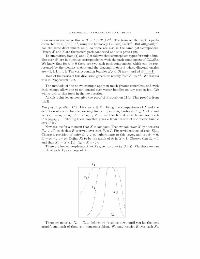
A GEOMETRIC INTRODUCTION TO K-THEORY 69
then we can rearrange this as β′ = h(0)βh(1)−1. The term on the right is path-connected to h(0)βh(0)−1, using the homotopy t 7→ h(0)βh(t)−1. But h(0)βh(0)−1
has the same determinant as β, so these are also in the same path-component.Hence, β′ and β are themselves path-connected and this proves (2).
To summarize, from (1) and (2) it follows that isomorphism types for rank n bun-dles over S1 are in bijective correspondence with the path components of GLn(R).We know that for n > 0 there are two such path components, which can be rep-resented by the identity matrix and the diagonal matrix J whose diagonal entriesare −1, 1, 1, . . . , 1. The corresponding bundles En(id, β) are n and M ⊕ (n− 1).
Most of the basics of this discussion generalize readily from S1 to Sk. We discussthis in Proposition 12.2.
The methods of the above example apply in much greater generality, and withlittle change allow one to get control over vector bundles on any suspension. Wewill return to this topic in the next section.
At this point let us now give the proof of Proposition 11.1. This proof is from[Ha2].
Proof of Proposition 11.1. Pick an x ∈ X. Using the compactness of I and thedefinition of vector bundle, we may find an open neighborhood U ⊆ X of x andvalues 0 = a0 < a1 < ... < an−1 < an = 1 such that E is trivial over eachU × [ai, ai+1]. Patching these together gives a trivialization of the vector bundleover U × I.
Now assume for a moment that X is compact. Then we can cover X by open setsU1, . . . , Un such that E is trivial over each Ui × I. Fix trivializations of each E|Ui .Choose a partition of unity φ1, . . . , φn subordinate to this cover, and set β0 = 0,βi = φ1 + . . .+ φi. Define Xi to be the graph of βi in X × I. Observe that βn = 1and thus Xn = X × 1, X0 = X × 0.
There are homeomorphisms X → Xi given by x 7→ (x, βi(x)). Via these we canthink of each Xi as a copy of X.
X0
X1
X3
X2
X4
There are maps fi : Xi → Xi−1 defined by “pushing down until you hit the nextgraph”, and each of these is a homeomorphism. We may restrict E over each Xi,
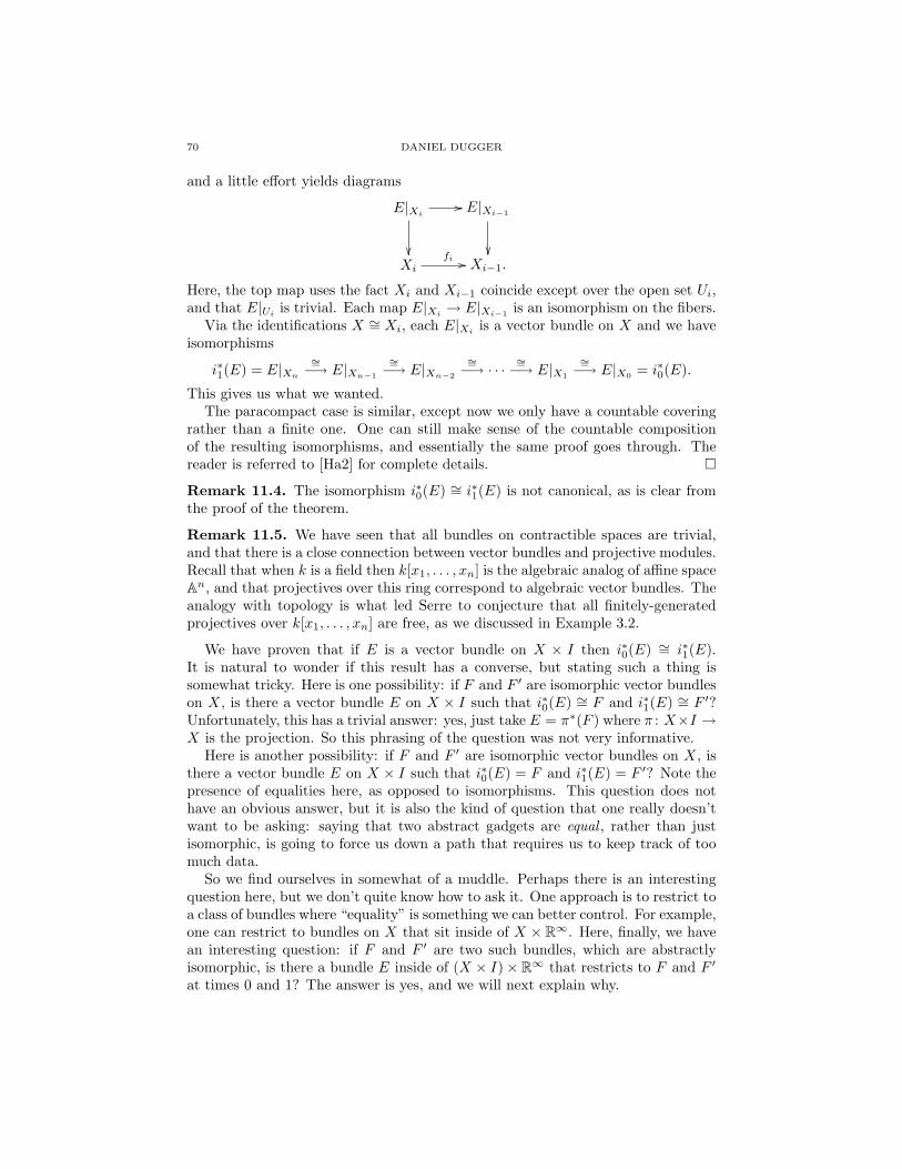
70 DANIEL DUGGER
and a little effort yields diagrams
E|Xi
// E|Xi−1
Xi
fi // Xi−1.
Here, the top map uses the fact Xi and Xi−1 coincide except over the open set Ui,and that E|Ui is trivial. Each map E|Xi → E|Xi−1 is an isomorphism on the fibers.
Via the identifications X ∼= Xi, each E|Xi is a vector bundle on X and we haveisomorphisms
i∗1(E) = E|Xn
∼=−→ E|Xn−1
∼=−→ E|Xn−2
∼=−→ · · ·∼=−→ E|X1
∼=−→ E|X0 = i∗0(E).
This gives us what we wanted.The paracompact case is similar, except now we only have a countable covering
rather than a finite one. One can still make sense of the countable compositionof the resulting isomorphisms, and essentially the same proof goes through. Thereader is referred to [Ha2] for complete details.
Remark 11.4. The isomorphism i∗0(E) ∼= i∗1(E) is not canonical, as is clear fromthe proof of the theorem.
Remark 11.5. We have seen that all bundles on contractible spaces are trivial,and that there is a close connection between vector bundles and projective modules.Recall that when k is a field then k[x1, . . . , xn] is the algebraic analog of affine spaceAn, and that projectives over this ring correspond to algebraic vector bundles. Theanalogy with topology is what led Serre to conjecture that all finitely-generatedprojectives over k[x1, . . . , xn] are free, as we discussed in Example 3.2.
We have proven that if E is a vector bundle on X × I then i∗0(E) ∼= i∗1(E).It is natural to wonder if this result has a converse, but stating such a thing issomewhat tricky. Here is one possibility: if F and F ′ are isomorphic vector bundleson X, is there a vector bundle E on X × I such that i∗0(E) ∼= F and i∗1(E) ∼= F ′?Unfortunately, this has a trivial answer: yes, just take E = π∗(F ) where π : X×I →X is the projection. So this phrasing of the question was not very informative.
Here is another possibility: if F and F ′ are isomorphic vector bundles on X, isthere a vector bundle E on X × I such that i∗0(E) = F and i∗1(E) = F ′? Note thepresence of equalities here, as opposed to isomorphisms. This question does nothave an obvious answer, but it is also the kind of question that one really doesn’twant to be asking: saying that two abstract gadgets are equal , rather than justisomorphic, is going to force us down a path that requires us to keep track of toomuch data.
So we find ourselves in somewhat of a muddle. Perhaps there is an interestingquestion here, but we don’t quite know how to ask it. One approach is to restrict toa class of bundles where “equality” is something we can better control. For example,one can restrict to bundles on X that sit inside of X × R∞. Here, finally, we havean interesting question: if F and F ′ are two such bundles, which are abstractlyisomorphic, is there a bundle E inside of (X × I)× R∞ that restricts to F and F ′
at times 0 and 1? The answer is yes, and we will next explain why.
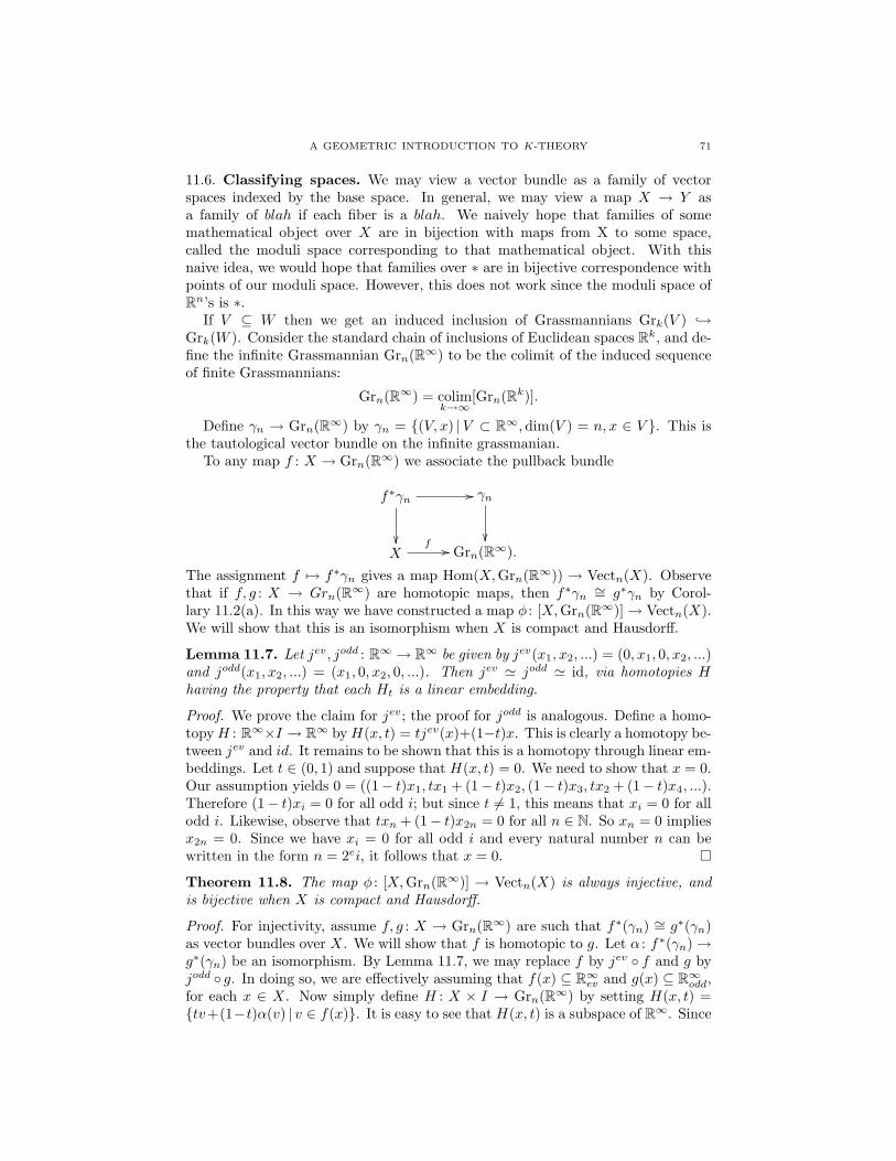
A GEOMETRIC INTRODUCTION TO K-THEORY 71
11.6. Classifying spaces. We may view a vector bundle as a family of vectorspaces indexed by the base space. In general, we may view a map X → Y asa family of blah if each fiber is a blah. We naively hope that families of somemathematical object over X are in bijection with maps from X to some space,called the moduli space corresponding to that mathematical object. With thisnaive idea, we would hope that families over ∗ are in bijective correspondence withpoints of our moduli space. However, this does not work since the moduli space ofRn’s is ∗.
If V ⊆ W then we get an induced inclusion of Grassmannians Grk(V ) →Grk(W ). Consider the standard chain of inclusions of Euclidean spaces Rk, and de-fine the infinite Grassmannian Grn(R∞) to be the colimit of the induced sequenceof finite Grassmannians:
Grn(R∞) = colimk→∞
[Grn(Rk)].
Define γn → Grn(R∞) by γn = (V, x) |V ⊂ R∞,dim(V ) = n, x ∈ V . This isthe tautological vector bundle on the infinite grassmanian.
To any map f : X → Grn(R∞) we associate the pullback bundle
f∗γn
// γn
X
f // Grn(R∞).
The assignment f 7→ f∗γn gives a map Hom(X,Grn(R∞)) → Vectn(X). Observethat if f, g : X → Grn(R∞) are homotopic maps, then f∗γn ∼= g∗γn by Corol-lary 11.2(a). In this way we have constructed a map φ : [X,Grn(R∞)]→ Vectn(X).We will show that this is an isomorphism when X is compact and Hausdorff.
Lemma 11.7. Let jev, jodd : R∞ → R∞ be given by jev(x1, x2, ...) = (0, x1, 0, x2, ...)and jodd(x1, x2, ...) = (x1, 0, x2, 0, ...). Then jev ' jodd ' id, via homotopies Hhaving the property that each Ht is a linear embedding.
Proof. We prove the claim for jev; the proof for jodd is analogous. Define a homo-topyH : R∞×I → R∞ byH(x, t) = tjev(x)+(1−t)x. This is clearly a homotopy be-tween jev and id. It remains to be shown that this is a homotopy through linear em-beddings. Let t ∈ (0, 1) and suppose that H(x, t) = 0. We need to show that x = 0.Our assumption yields 0 = ((1− t)x1, tx1 + (1− t)x2, (1− t)x3, tx2 + (1− t)x4, ...).Therefore (1− t)xi = 0 for all odd i; but since t 6= 1, this means that xi = 0 for allodd i. Likewise, observe that txn + (1− t)x2n = 0 for all n ∈ N. So xn = 0 impliesx2n = 0. Since we have xi = 0 for all odd i and every natural number n can bewritten in the form n = 2ei, it follows that x = 0.
Theorem 11.8. The map φ : [X,Grn(R∞)] → Vectn(X) is always injective, andis bijective when X is compact and Hausdorff.
Proof. For injectivity, assume f, g : X → Grn(R∞) are such that f∗(γn) ∼= g∗(γn)as vector bundles over X. We will show that f is homotopic to g. Let α : f∗(γn)→g∗(γn) be an isomorphism. By Lemma 11.7, we may replace f by jev f and g byjodd g. In doing so, we are effectively assuming that f(x) ⊆ R∞ev and g(x) ⊆ R∞odd,for each x ∈ X. Now simply define H : X × I → Grn(R∞) by setting H(x, t) =tv+(1−t)α(v) | v ∈ f(x). It is easy to see that H(x, t) is a subspace of R∞. Since

72 DANIEL DUGGER
f(x) and g(x) are disjoint one readily argues that H(x, t) is n-dimensional, for all t.So we really do have a homotopy, and clearly H0 = g and H1 = f . CONTINUITYOF H? PICTURE HERE
For surjectivity, assume X is compact and Hausdorff and let E → X be a vectorbundle of rank n. Then by Proposition 9.5 there exists an embedding j : E → N,for large enough N (this is where we use the assumption on X). Note that N =X × RN ⊆ X × R∞. Now define f : X → Grn(R∞) by f(x) = j(Ex) ⊆ RN ⊆ R∞.It is left to the reader to check that f is continuous and that f∗(γn) ∼= E.
11.9. Stabilization of vector bundles. Here is a simple application of classifyingspaces that we will occasionally find useful. Fix a space X. If E → X is a vectorbundle of rank n, then of course E ⊕ 1 is a vector bundle of rank n+ 1. We get asequence of maps
Vect0(X) ⊕1−→ Vect1(X) ⊕1−→ Vect2(X) ⊕1−→ · · ·Are these maps injective? Surjective? Are there more and more isomorphismclasses of vector bundles as one goes up in rank, or is it the case that all “large”rank vector bundles actually come from smaller ones via addition of a trivial bundle?A homotopical analysis of classifying spaces allow us give some partial answers here.We handle both the case of real and complex bundles:
Proposition 11.10. Let X be a finite-dimensional CW-complex. For real vectorbundles, Vectn(X)→ Vectn+1(X) is a bijection for n ≥ dimX+1 and a surjectionfor n = dimX. For complex bundles, VectC
n(X) → VectCn+1(X) is a bijection for
n ≥ 12 dimX and a surjection for n ≥ 1
2 (dimX − 1).
Proof. The map Vectn(X) → Vectn+1(X) is represented by a map of spacesf : Grn(R∞)→ Grn+1(R∞). A little thought shows this to be the map that sendsa subspace V ⊆ R∞ to R ⊕ V ⊆ R ⊕ R∞ and then uses a fixed isomorphismR ⊕ R∞ ∼= R∞ to obtain a point in Grn+1(R∞). To establish the proposition we
must analyze when [X,Grn(R∞)]f∗−→ [X,Grn+1(R∞)] is injective/surjective.
Now, the inclusion Grn(R∞) → Grn+1(R∞) is n-connected. This can be arguedin different ways, but one way is to examine the Schubert cell decompositions ofeach space and observe that they are identical until one reaches dimension n + 1.This connectivity result implies that [B,Grn(R∞)] → [B,Grn+1(R∞)] is bijectivefor CW-complexes with dimB ≤ n − 1, and surjective for CW-complexes withdimB = n. We simply apply this to B = X.
For the complex case, Grn(C∞) → Grn+1(C∞) is now (2n + 1)-connected. Sowe get the analogous bijection for CW-complexes B of dimension at most 2n, andthe surjection when dimB = 2n+ 1.
12. Vector bundles on spheres
In this section we explore the set of isomorphism classes Vectn(Sk) for variousvalues of k and n. There are two important points. First, for a fixed k thesesets stablize for n 0. Secondly, Bott was able to compute these stable valuescompletely and found an 8-fold periodicity (with respect to k) in the case of realvector bundles, and a 2-fold periodicity in the case of complex bundles. Bott’speriodicity theorems are of paramount importance in modern algebraic topology.
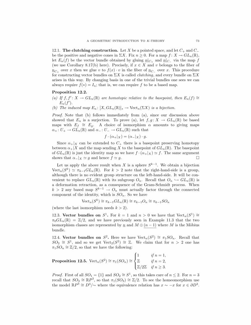
A GEOMETRIC INTRODUCTION TO K-THEORY 73
12.1. The clutching construction. LetX be a pointed space, and let C+ and C−be the positive and negative cones in ΣX. Fix n ≥ 0. For a map f : X → GLn(R),let En(f) be the vector bundle obtained by gluing n|C+ and n|C− via the map f(we use Corollary 8.17(b) here). Precisely, if x ∈ X and v belongs to the fiber ofnC+
over x then we glue v to f(x) · v in the fiber of nC− over x. This procedurefor constructing vector bundles on ΣX is called clutching , and every bundle on ΣXarises in this way. By changing basis in one of the trivial bundles one sees we canalways require f(∗) = In; that is, we can require f to be a based map.
Proposition 12.2.(a) If f, f ′ : X → GLn(R) are homotopic relative to the basepoint, then En(f) ∼=
En(f ′).(b) The induced map En : [X,GLn(R)]∗ → Vectn(ΣX) is a bijection.
Proof. Note that (b) follows immediately from (a), since our discussion aboveshowed that En is a surjection. To prove (a), let f, g : X → GLn(R) be basedmaps with Ef ∼= Eg. A choice of isomorphism α amounts to giving mapsα+ : U+ → GLn(R) and α− : U− → GLn(R) such that
f · (α+|X) = (α−|X) · g.Since α+|X can be extended to C+ there is a basepoint preserving homotopy
between α+|X and the map sending X to the basepoint of GLn(R). The basepointof GLn(R) is just the identity map so we have f · (α+|X) ' f . The same argumentshows that α−|X ' g and hence f ' g.
Let us apply the above result when X is a sphere Sk−1. We obtain a bijectionVectn(Sk) ' πk−1GLn(R). For k > 2 note that the right-hand-side is a group,although there is no evident group structure on the left-hand-side. It will be con-venient to replace GLn(R) with its subgroup On. Recall that On → GLn(R) isa deformation retraction, as a consequence of the Gram-Schmidt process. Whenk > 2 any based map Sk−1 → On must actually factor through the connectedcomponent of the identity, which is SOn. So we have
Vectn(Sk) ∼= πk−1GLn(R) ∼= πk−1On ∼= πk−1SOn
(where the last isomorphism needs k > 2).
12.3. Vector bundles on S1. For k = 1 and n > 0 we have that Vectn(S1) ∼=π0GLn(R) = Z/2, and we have previously seen in Example 11.3 that the twoisomorphism classes are represented by n and M ⊕ (n− 1) where M is the Mobiusbundle.
12.4. Vector bundles on S2. Here we have Vectn(S2) ∼= π1SOn. Recall thatSO2
∼= S1, and so we get Vect2(S2) ∼= Z. We claim that for n > 2 one hasπ1SOn ∼= Z/2, so that we have the following:
Proposition 12.5. Vectn(S2) ∼= π1(SOn) ∼=
1 if n = 1,Z if n = 2,Z/2Z if n ≥ 3.
Proof. First of all SO1 = 1 and SO2∼= S1, so this takes care of n ≤ 2. For n = 3
recall that SO3∼= RP 3, so that π1(SO3) ∼= Z/2. To see the homeomorphism use
the model RP 3 ∼= D3/∼ where the equivalence relation has x ∼ −x for x ∈ ∂D3.
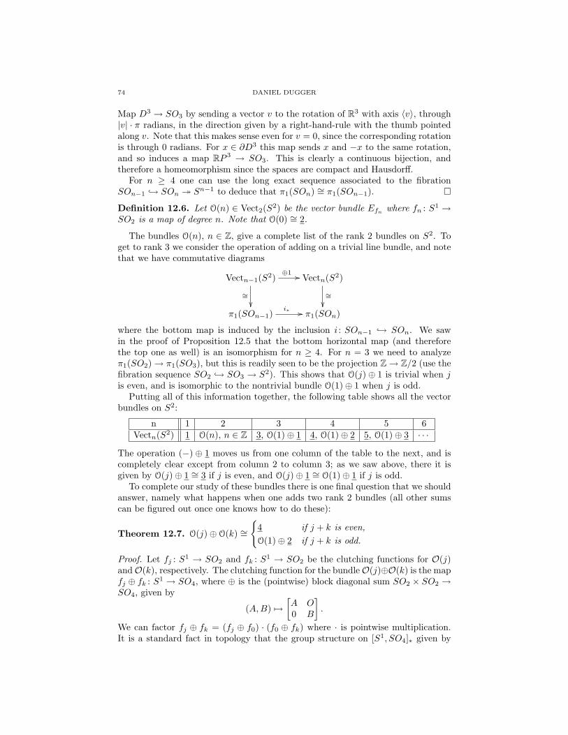
74 DANIEL DUGGER
Map D3 → SO3 by sending a vector v to the rotation of R3 with axis 〈v〉, through|v| · π radians, in the direction given by a right-hand-rule with the thumb pointedalong v. Note that this makes sense even for v = 0, since the corresponding rotationis through 0 radians. For x ∈ ∂D3 this map sends x and −x to the same rotation,and so induces a map RP 3 → SO3. This is clearly a continuous bijection, andtherefore a homeomorphism since the spaces are compact and Hausdorff.
For n ≥ 4 one can use the long exact sequence associated to the fibrationSOn−1 → SOn Sn−1 to deduce that π1(SOn) ∼= π1(SOn−1).
Definition 12.6. Let O(n) ∈ Vect2(S2) be the vector bundle Efn where fn : S1 →SO2 is a map of degree n. Note that O(0) ∼= 2.
The bundles O(n), n ∈ Z, give a complete list of the rank 2 bundles on S2. Toget to rank 3 we consider the operation of adding on a trivial line bundle, and notethat we have commutative diagrams
Vectn−1(S2)⊕1 //
∼=
Vectn(S2)
∼=
π1(SOn−1)i∗ // π1(SOn)
where the bottom map is induced by the inclusion i : SOn−1 → SOn. We sawin the proof of Proposition 12.5 that the bottom horizontal map (and thereforethe top one as well) is an isomorphism for n ≥ 4. For n = 3 we need to analyzeπ1(SO2)→ π1(SO3), but this is readily seen to be the projection Z→ Z/2 (use thefibration sequence SO2 → SO3 → S2). This shows that O(j)⊕ 1 is trivial when jis even, and is isomorphic to the nontrivial bundle O(1)⊕ 1 when j is odd.
Putting all of this information together, the following table shows all the vectorbundles on S2:
n 1 2 3 4 5 6Vectn(S2) 1 O(n), n ∈ Z 3, O(1)⊕ 1 4, O(1)⊕ 2 5, O(1)⊕ 3 · · ·
The operation (−) ⊕ 1 moves us from one column of the table to the next, and iscompletely clear except from column 2 to column 3; as we saw above, there it isgiven by O(j)⊕ 1 ∼= 3 if j is even, and O(j)⊕ 1 ∼= O(1)⊕ 1 if j is odd.
To complete our study of these bundles there is one final question that we shouldanswer, namely what happens when one adds two rank 2 bundles (all other sumscan be figured out once one knows how to do these):
Theorem 12.7. O(j)⊕ O(k) ∼=
4 if j + k is even,O(1)⊕ 2 if j + k is odd.
Proof. Let fj : S1 → SO2 and fk : S1 → SO2 be the clutching functions for O(j)andO(k), respectively. The clutching function for the bundleO(j)⊕O(k) is the mapfj ⊕ fk : S1 → SO4, where ⊕ is the (pointwise) block diagonal sum SO2 × SO2 →SO4, given by
(A,B) 7→[A O0 B
].
We can factor fj ⊕ fk = (fj ⊕ f0) · (f0 ⊕ fk) where · is pointwise multiplication.It is a standard fact in topology that the group structure on [S1, SO4]∗ given by

A GEOMETRIC INTRODUCTION TO K-THEORY 75
pointwise multiplication agrees with the group structure given by concatenationof loops (this is true with SO4 replaced by any topological group). Note that thehomotopy classes of f0⊕fk and fk⊕f0 are the same, since these clutching functionsgive rise to isomorphic bundles. So we have
[fj ⊕ fk] = [fj ⊕ f0] + [fk ⊕ f0]where this is a statement abouts sums of homotopy classes in π1(SO4).
But π1(SO4) = Z/2. The function fj ⊕ f0 is the nontrivial element of π1SO4
precisely when j is odd, and similarly for fk ⊕ f0. It follows that the sum of theseelements is trivial/non-trivial when j + k is even/odd.
12.8. Vector bundles on S3. Now we have to calculate π2SOn. This is trivialfor n ≤ 2 (easy), and for n = 3 it also trivial: use SO3
∼= RP 3 and the fibrationsequence Z/2 → S3 RP 3. Finally, the fibration sequences SOn−1 → SOn Sn−1 now show that π2SOn = 0 for all n. We have proven
Proposition 12.9. Vectn(S3) ∼= π2(SOn) ∼= 0. That is, every vector bundle on S3
is trivializable.
12.10. Vector bundles on S4. Once again, we are reduced to calculating π3SOn.Eventually one expects to get stuck here, but so far we have been getting luckyso let’s keep trying. The group is trivial for n ≤ 2, and for n = 3 it is Z usingSO3
∼= RP 3 and Z/2→ S3 → RP 3. Next look at the long exact homotopy sequencefor the fibration SO3 → SO4 → S3:
· · · → Z/2 = π4(S3)→ Z→ π3SOr → Z→ π2(SO3) = 0.
It follows that π3SO4∼= Z2. Next do the same thing for SO4 → SO5 → S4:
Z = π4SO4 → π3SO4 → π3SO5 → 0.
Unfortunately we cannot go further without calculating the map π4S4 → π3SO4,
which is Z→ Z2. So now we are indeed stuck, unless we can resolve this issue. Note,however, that the fibrations SOn−1 → SOn → Sn−1 show that π3SO5 = π3SOnfor n ≥ 5, so once we’ve figured this one out we know everything. We will notjustify it here, but it turns out that the map Z → Z2 is an inclusion. So we getthat
Proposition 12.11. Vectn(S4) ' π3(SOn) ∼=
1 n ≤ 2Z n = 3Z2 n = 4Z n > 5.
With some additional work one can write down a table of all bundles on S4,much as we did for S2, and figure out how all the direct sums behave. We won’tbother with this.
12.12. Vector bundles on Sk. Although we can not readily do the calculationsfor k > 4, at this point one sees the general pattern. One must calculate πk−1SOnfor each n, and these groups vary for a while but eventually stabilize. In fact,πiSOn ∼= πiSOn+1 for i + 1 < n. The calculation of these stable groups was animportant problem back in the 1950s, that was eventually solved by Bott.
Let us phrase things as follows. Consider the inclusions
O1 → O2 → O3 → · · ·

76 DANIEL DUGGER
that send a matrix A to[A 00 1
]. The colimit of this sequence is denoted O and
called the stable orthogonal group. The homotopy groups of O are the stablevalues that we encountered above. We computed the first few: π0O = Z/2, π1O =Z/2, π2O = 0. And we stated, without proof, that π3O = Z. Bott’s calculationshowed the following:
i 0 1 2 3 4 5 6 7 8 9 10 11 12 13 14πiO Z/2 Z/2 0 Z 0 0 0 Z Z/2 Z/2 0 Z 0 0 Z
The pattern is 8-fold periodic: πi+8O ∼= πiO for all i ≥ 0. One is supposed toremember the pattern of groups to the tune of “Twinkle, Twinkle, Little Star”:
zee - two - zee - two - ze - ro - zee ze - ro - ze - ro - ze - ro - zee.
We will eventually have to understand Bott’s computations at a deeper level; inparticular, we will need to get our hands on explicit generators. But for now wewill just accept that the values are as given above.
12.13. Complex vector bundles on spheres. One can repeat the above analysisfor complex vector bundles on a sphere. One finds that
VectCn(Sk) ∼= πk−1(GLn(C)) ∼= πk−1(Un),
where Un → GLn(C) is the unitary group. Analogously to the real case, one hasfiber bundles Un−1 → Un S2n−1. Using that U1
∼= S1 one can again computeVectC
n(Sk) for small values of k. Here is what you get:
n 1 2 3 4 5 6 · · ·Vectn(S1) 0 0 0 0 0 0 · · ·Vectn(S2) Z Z Z Z Z Z · · ·Vectn(S3) 0 0 0 0 0 0 · · ·Vectn(S4) 0 Z Z Z Z Z · · ·Vectn(S5) 0 Z/2 0 or Z/2 0 or Z/2 0 or Z/2 0 or Z/2 · · ·
The stable value in the last row turns out to be 0, although one cannot figure thisout without computing a connecting homomorphism in the long exact homotopysequence.
The fiber bundles Un−1 → Un S2n−1 again imply that πiUn stabilizes as ngrows. In fact, πiUn ∼= πiUn+1 for n > i
2 . We can write the stable value as πiUwhere U is the infinite unitary group defined as the colimit of
U1 → U2 → U3 → · · ·Bott computed the homotopy groups of U to be 2-fold periodic, with
πiU =
Z if i is odd0 if i is even.
Again, for now we will just accept this result; but eventually we will have to un-derstand the computation in more detail, and in particular we will need to get ourhands on specific generators.
A GEOMETRIC INTRODUCTION TO K-THEORY 77
13. Topological K-theory
For a compact and Hausdorff space X, let KO(X) denote the Grothendieckgroup of real vector bundles over X. Swan’s Theorem gives that KO(X) ∼=Kalg(C(X)), where the latter denotes the Grothendieck group of finitely-generatedprojectives. We can repeat this definition for both complex and quaternionic bun-dles, to define groups KU(X) and KSp(X), respectively. The group KU(X) ismost commonly just written K(X) for brevity. In this section we start to developthe general theory of these groups, mostly concentrating on KO(X) because thestory is very analogous in the three cases.
Until we explicitly mention otherwise, all spaces in this section are assumed tobe compact and Hausdorff.
13.1. Initial observations on KO. Observe that KO(−) is a contravariant func-tor: if f : X → Y then f∗ : KO(Y ) → KO(X) sends [E] to [f∗E]. In particular,the squash map p : X → ∗ yields a split-inclusion p∗ : KO(∗)→ KO(X), where thesplitting is induced by any choice of basepoint in X. One has KO(∗) ∼= Z, so Z is adirect summand of KO(X). To analyze the complement we can take two differentapproaches:
Definition 13.2. For x ∈ X let KO (X,x) = ker[KO(X) i∗−→ KO(x)] wherei : x → X. Further, define KOst(X) = KO(X)/p∗KO(∗).
The group KO (X,x) is called the reduced KO-group of the pointed space X.We call KOst(X) the Grothendieck group of stable vector bundles on X.The reason for the latter terminology will be clear momentarily. These two groupsare isomorphic; algebraically, this is coming from the split-exact sequence
0→ KO(∗)→ KO(X)→ KOst → 0.
If i : x → X is the inclusion then i∗ is a splitting for the first map in the sequence.One gets an isomorphism between KOst(X) and ker i∗ in the evident way, bysending a class [E] to [E]− p∗i∗[E]. This isomorphism is used so frequently that itis worth recording more visibly:
KOst(X) ∼= KO (X,x) via [E] 7→ [E]− [rankx(E)].(13.3)
Remark 13.4. Both KOst(X) and KO (X,x) appear often in algebraic topology,and topologists are somewhat cavalier about mixing them up. We give here oneexample where this can cause confusion.
Tensor product of bundles makes KO(X) into a ring, via the formula [E] · [F ] =[E ⊗ F ] and extending linearly. Then KO (X,x) is an ideal of this ring. ThereforeKOst(X) may be given a product via the above isomorphism, but this productis not [E] · [F ] = [E ⊗ F ]. Indeed, it is clear that this definition would not beinvariant under E 7→ E ⊕ 1. The product on KOst(X) is instead [E] · [F ] =[E ⊗ F ]− (rankE)[F ]− (rankF )[E] + (rankE)(rankF ).
We offer the following alternative description of KOst(X). Let Vect(X) be theset of isomorphism classes of vector bundles on X, and impose the equivalencerelation E ' E ⊕ 1 for every vector bundle E. The set of equivalence classesis obviously a monoid under direct sum (this would be true even without takingequivalence classes), but it is actually more than a monoid: it is a group. To see

78 DANIEL DUGGER
this, recall that if E is any vector bundle over X then there exists an embeddingE → N for sufficiently large N (Proposition 9.5). If Q is the quotient then we havethe exact sequence 0 → E → N → Q → 0, which is split by Proposition 9.2. SoE ⊕Q ∼= N . Yet N = 0 under our equivalence relation, and so E has an additiveinverse. It is easy to see that KOst(X) is precisely this set of equivalence classes.
Finally, here is a third description of KOst(X). Consider the chain of maps
Vect0(X) ⊕1−→ Vect1(X) ⊕1−→ Vect2(X) ⊕1−→ · · ·The colimit is clearly the set of equivalence classes described in the preceding para-graph, and therefore coincides with KOst(X).
Recall that Vectn(X) = [X,Grn(R∞)], and one easily sees that the ⊕1 map isrepresented by the map of spaces
Grn(R∞) −→ Grn+1(R⊕ R∞) = Grn+1(R∞)
that sends a subspace U ⊆ R∞ to R ⊕ U ⊆ R ⊕ R∞. Let Gr∞(R∞) denote thecolimit of these maps
Gr1(R∞) ⊕1−→ Gr2(R∞) ⊕1−→ Gr3(R∞) ⊕1−→ · · ·(we really want the homotopy colimit, if you know what that is, but in this casethe colimit has the same homotopy type and is good enough). You might recallthat Grn(R∞) is also called BOn, and likewise Gr∞(R∞) is also called BO.
Then (for compact Hausdorff spaces X) we have a bijection
colimn
[X,Grn(R∞)] −→ [X,Gr∞(R∞)].
So we have learned that KOst(X) ' [X,BO].If X has a basepoint then we can consider [X,BO]∗ instead of [X,BO]. There
is the evident map [X,BO]∗ → [X,BO]. Typically there would be no reason forthis to be a bijection, but BO is a path-connected H-space: and in this setting themap is a bijection. So in fact we can write
KOst(X) ' [X,BO]∗.
NOTE: PROBLEM WITH X = S0.Applying this in particular to X = Sk we have that for k ≥ 1
KO (Sk) ∼= KOst(Sk) ∼= [Sk, BO] ∼= [Sk, BO]∗ = πk(BO) = πk−1(O).
The calculations of Bott therefore give us the values of KO (Sk). For k = 0 observethat KO(S0) = KO(∗ t ∗) ∼= Z⊕ Z, so we have KO (S0) ∼= Z. This lets us fill outthe table:
Table 13.4. Reduced KO-theory of spheres
k 0 1 2 3 4 5 6 7 8 9 10 11 · · ·KO (Sk) Z Z/2 Z/2 0 Z 0 0 0 Z Z/2 Z/2 0 · · ·
Now let X be an arbitrary CW-complex, not necessarily compact. We define
KO(X) = [X+,Z×BO]∗ = [X,Z×BO],
where X+ denotes X with a basepoint added. For a pointed space X we defineKO (X) = [X,Z×BO]∗.
A GEOMETRIC INTRODUCTION TO K-THEORY 79
As we have seen it before, Bott Periodicity shows that the homotopy groupsof Z × BO are 8-fold periodic. This is a consequence of the following strongerstatement:
Theorem 13.5 (Bott Periodicity, Strong version). There is a weak equivalence ofspaces Z×BO ' Ω8(Z×BO).
Using Bott Periodicity we can then calculate that for every pointed space X onehas
KO (Σ8X) = [Σ8X,Z×BO]∗ = [X,Ω8(Z×BO)]∗ = [X,Z×BO]∗ = KO (X).
Remark 13.6. In the complex case, Bott Periodicity gives the weak equivalenceZ×BU ' Ω2(Z×BU). Consequently one obtains K(Σ2X) ∼= K(X) for all pointedspaces X.
13.7. K-theory as a cohomology theory. WhenX is compact and Hausdorff wehave seen that KO(X) ∼= [X+,Z×BO]∗, where X+ is X with a disjoint basepointadded. The point of this isomorphism is that it immediately gives us several toolsfor computing KO(X) that we didn’t have before. These are tools that work forhomotopy classes of maps in reasonable generality, so let us discuss them in thatbroader context.
Let X and Z be pointed spaces. Then [X,Z]∗ is just a pointed set, but if wesuspend the space in the domain then we get a bit more structure: [ΣX,Z]∗ is agroup, where ΣX is the reduced suspension of X. One way to see this is to collapsethe equatorial copy of X in ΣX, to get ΣX ∨ ΣX; write this collapse map as
∇ : ΣX → ΣX ∨ ΣX.
The operation on [ΣX,Z]∗ is defined by precomposing the wedge of two homotopyclasses with ∇. With some trouble one checks that ΣX is a cogroup object in thehomotopy category of pointed spaces, which yields that [ΣX,Z]∗ is a group.
Here is another way to think about this, which relates it to something we alreadyknow. Let F (X,Z) be the set of functions from X to Z, equipped with the compactopen topology. We can write
[ΣX,Z]∗ = [S1, F (X,Z)]∗ = π1(F (X,Z))
where the basepoint of F (X,Z) is the map sending all of X to the basepoint of Z.Now just use that π1(F (X,Z)) is a group.
When k ≥ 2 then we have [ΣkX,Z]∗ = πk(F (X,Z)) by a similar argument, andso [ΣkX,Z]∗ is an abelian group. Alternatively, one proves that now ΣkX is acocommutative cogroup object in the homotopy category.
Similar results are obtained by putting conditions on Z rather than X. If Z isa loop space, say Z ' ΩZ1, then [X,Z]∗ ∼= [X,ΩZ1]∗ ∼= [ΣX,Z1]∗, and this is agroup by the above arguments. Similarly, if Z is a k-fold loop space for k ≥ 2, sayZ ' ΩkZ1, then [X,Z]∗ ∼= [Σk, Z1]∗ and this is an abelian group.
Homotopy classes of maps into a fixed space Z always give rise to exact sequences:
Proposition 13.8. Let X,Y be pointed spaces, and let f : X → Y be a pointedmap. Consider the mapping cone Cf and the natural map p : Y → Cf . For anypointed space Z, the sequence of pointed sets [X,Z]∗ ← [Y, Z]∗ ← [Cf,Z]∗ is exactin the middle.

80 DANIEL DUGGER
Proof. Let h : Y → Z and suppose h f is homotopic to the constant map. Choosea pointed homotopy H : X × I → Z so that H(X × 1) = ∗. Then H induces amap from CX → Z. Let g : Cf → Z be given by H on CX and h on Y . Thenclearly g p = h.
Given f : X → Y we form the mapping cone Cf , which comes to us with aninclusion j0 : Y → Cf . Next form the mapping cone on i, which comes with aninclusion j1 : Cf → Cj0. Keep doing this forever to get the sequence of spacesX → Y → Cf → Cj0 → Cj1 → · · · depicted below:
Note that Cj0 ' ΣX and Cj1 ' ΣY (this is clear from the pictures). Up to signthe map Cj0 → Cj1 is just Σf , so that the sequence of spaces becomes periodic:
X → Y → Cf → ΣX → ΣY → Σ(Cf)→ Σ2X → . . .
This is called the Puppe sequence. Note that the composition of two subse-quent maps is null-homotopic, and that every three successive terms form a cofibersequence.
Now let Z be a fixed space and apply [−, Z]∗ to the Puppe sequence. We obtainthe sequence of pointed sets
[X,Z]∗ ← [Y, Z]∗ ← [Cf,Z]∗ ← [ΣX,Z]∗ ← [ΣY, Z]∗ ← [Σ(Cf), Z]∗ ← . . .
By Proposition 13.8 this sequence is exact at every spot where this makes sense(everywhere except at [X,Z]∗). At the left end this is just an exact sequence ofpointed sets, but as one moves to the right at some point it becomes an exactsequence of groups (namely, at [ΣY, Z]∗). As one moves further to the right, itbecomes an exact sequence of abelian groups by the time one gets to [Σ2Y, Z]∗.
If Z ' ΩZ1 then we can extend the above sequence a little further to the left,by noticing that the sequences for [−, Z1]∗ and [−, Z]∗ mesh together:
[X,Z1]∗ [Y, Z1]∗oo [Cf,Z1]∗oo [ΣX,Z1]∗oo [ΣY, Z1]∗oo [Σ(Cf), Z1]oo oo
[X,ΩZ1]∗ [Y,ΩZ1]∗oo [Cf,ΩZ1]oo oo
[X,Z]∗ [Y, Z]∗oo [Cf,Z]oo oo
Note that the leftmost cycle of the original sequence, which we had thought con-sisted just of pointed sets, in fact consisted of groups! If in turn we have Z1 ' ΩZ2
then we can play this game again and extend the sequence one more cycle to theleft, and so forth. If we are really lucky then we can do this forever:
A GEOMETRIC INTRODUCTION TO K-THEORY 81
Definition 13.9. An infinite loop space is a space Z0 together with spacesZ1, Z2, Z3, . . . and weak homotopy equivalences Zn ' ΩZn+1 for all n ≥ 0.
Note that if Z is an infinite loop space then we really do get a long exactsequence—infinite in both directions—consisting entirely of abelian groups, hav-ing the form
· · · ← [Cf,Zi+1]← [X,Zi]∗ ← [Y, Zi]∗ ← [Cf,Zi]∗ ← [X,Zi−1]← · · ·where it is convenient to use the indexing convention Z−n = ΩnZ for n > 0.
This situation is very reminiscent of a long exact sequence in cohomology, so letus adopt the following notation: write
EiZ(X) = [X+, Zi]∗ =
[X+, Zi]∗ i ≥ 0,[Σ−i(X+), Z0]∗ i < 0.
For an inclusion of subspaces j : A → X write
EiZ(X,A) = [Cj, Zi]+ =
[Cj, Zi]∗ i ≥ 0,[Σi(Cj), Z0]∗ i < 0.
It is not hard to check that this is a generalized cohomology theory. So we get ageneralized cohomology theory whenever we have an infinite loop space. (You mayknow that it works the other way around, too: every generalized cohomology comesfrom an infinite loop space. But we won’t need that fact here.)
For us the importance of all of this is that by Bott’s theorem we have
Z×BO ' Ω8(Z×BO) ' Ω16(Z×BO) ' . . . .Thus, Z×BO is an infinite loop space and the above machinery applies. We obtaina cohomology theory KO∗. Moreover, periodicity gives us that KOi+8(X,A) ∼=KOi(X,A), for any i.
This all works in the complex case as well. There we have Z×BU ' Ω2(Z×BU),so Z×BU is again an infinite loop space. We get a cohomology theory K∗ that is2-fold periodic.
13.10. Afterward. The point of this section was to construct the cohomologytheories KO and K, having the properties that when X is compact and Hausdorffthe groups KO0(X) and K0(X) coincide with the Grothendieck groups of real andcomplex vector bundles over X. We have now accomplished this! We will spendthe rest of these notes exploring what one can do with such cohomology theories,i.e., what they are good for. We have already said that one thing they are goodfor is calculation; we close this section with an example demonstrating the benefitsand limitations here.
Let us try to compute KO(RP 2). Recall the ubiquitous decompositionKO(RP 2) = Z ⊕ KO (RP 2) = Z ⊕ KOst(RP 2). Next use the fact that RP 2
can be built by attaching a 2-cell to RP 1 = S1, where the attaching map wraps S1
around itself twice. That is, RP 2 is the mapping cone for S1 2−→ S1. The Puppesequence for this map looks like
S1 2−→ S1 −→ RP 2 −→ S2 2−→ S2 −→ · · ·hence we have an exact sequence
← · · · ← KO (S1)← KO (S1)← KO (RP 2)← KO (S2)← KO (S2)← · · ·
82 DANIEL DUGGER
Note that this is just the long exact sequence for the pair (RP 2,RP 1) in KO -cohomology, where we are using the identification KO (S2) = KO 0(S2) =KO−1(S1).
We know KO (Sk) for all k ≥ 0, so the above sequence becomes
Z/2← Z/2← KO (RP 2)← Z/2← Z/2where both maps Z/2 ← Z/2 are multiplication by 2, i.e. the 0 map. Hence wehave a short exact sequence
0← Z/2← KO (RP 2)← Z/2← 0,(13.11)
and so either KO (RP 2) = (Z/2)2 or KO (RP 2) = Z/4. It remains to decide whichone.
The short exact sequence in (13.11) is really
0←− KO (S1) i∗←− KO (RP 2)p∗←− KO (S2)←− 0.
We have previously seen that the generator of KO 0(S1) = KOst(S1) correspondsto the Mobius bundle [M ], and the generator of KO (S2) = KOst(S2) is [O(1)],the rank 2 bundle whose clutching map is the isomomorphism S1 → SO(2). Theimage of [O(1)] in KO 0(RP 2) is p∗O(1), where p : RP 2 → S2 is the projection.
We happen to know one bundle on RP 2, the tautological line bundle γ. Whenwe restrict γ to RP 1 we get M , and so [γ] is a preimage for [M ] under i∗. We needto decide if 2[γ] = 0 in KOst(RP 2); if it is, then KO (RP 2) ∼= (Z/2)2 and if it isnot then KO (RP 2) ∼= Z/4. So the question becomes: is γ ⊕ γ stably trivial?
The answer turns out to be that γ ⊕ γ is not stably trivial; this is an elemen-tary exercise using characteristic classes (Stiefel-Whitney classes), but we have notdiscussed such techniques yet—see Section 23.8 below for complete details. Fornow we will just accept this fact, and conclude that KO (RP 2) ∼= Z/4. Note thatthis calculation demonstrates an important principle to keep in mind: often themachinery of cohomology theories get you a long way, but not quite to the end,and one has to do some geometry to complete the calculation.
There is a better way to think about this calculation, and we can’t resist pointingit out even though it won’t make complete sense yet. But it ties in to intersectiontheory, which is our overarching theme in these notes. In our discussion above weused KOst(RP 2) as our model for KO (RP 2), but let us change perspective anduse the model that is the kernel of KO(RP 2) → KO(∗), for some chosen base-point. Recall that [E] in KOst(RP 2) corresponds to [E] − rank(E) in KO (RP 2);so the class we wrote as [γ] is [γ] − 1 in the shifted perspective, and we need todecide if 2([γ]− 1) = 0 in KO(RP 2). The element 1− [γ] should be thought of ascorresponding to a chain complex of vector bundles
0→ γ → 1→ 0,
and thinking of it this way one finds that it plays the role of the K-theoreticfundamental class of the submanifold RP 1 → RP 2. Then (1 − [γ])2 representsthe self-intersection product of RP 1 inside RP 2, which we know is a point by thestandard geometric argument (shown in the picture below, depicting an RP 1 anda small perturbation of it)):
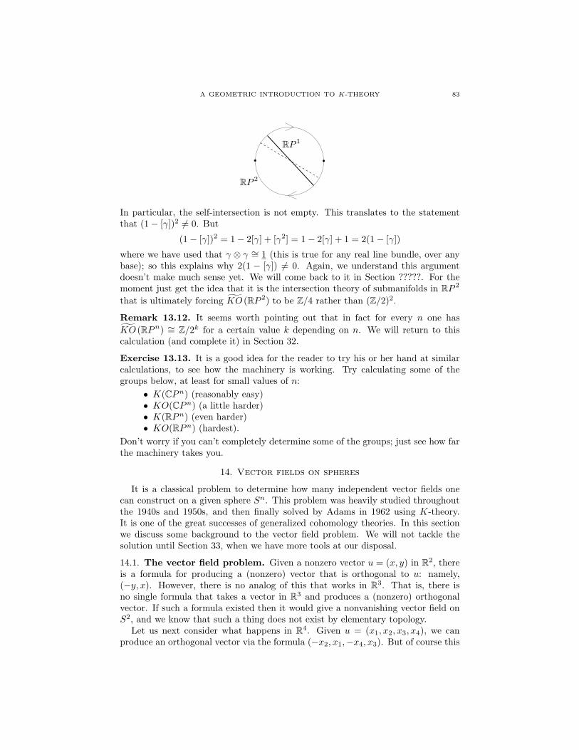
A GEOMETRIC INTRODUCTION TO K-THEORY 83
RP 2
RP 1
In particular, the self-intersection is not empty. This translates to the statementthat (1− [γ])2 6= 0. But
(1− [γ])2 = 1− 2[γ] + [γ2] = 1− 2[γ] + 1 = 2(1− [γ])
where we have used that γ ⊗ γ ∼= 1 (this is true for any real line bundle, over anybase); so this explains why 2(1 − [γ]) 6= 0. Again, we understand this argumentdoesn’t make much sense yet. We will come back to it in Section ?????. For themoment just get the idea that it is the intersection theory of submanifolds in RP 2
that is ultimately forcing KO (RP 2) to be Z/4 rather than (Z/2)2.
Remark 13.12. It seems worth pointing out that in fact for every n one hasKO (RPn) ∼= Z/2k for a certain value k depending on n. We will return to thiscalculation (and complete it) in Section 32.
Exercise 13.13. It is a good idea for the reader to try his or her hand at similarcalculations, to see how the machinery is working. Try calculating some of thegroups below, at least for small values of n:
• K(CPn) (reasonably easy)• KO(CPn) (a little harder)• K(RPn) (even harder)• KO(RPn) (hardest).
Don’t worry if you can’t completely determine some of the groups; just see how farthe machinery takes you.
14. Vector fields on spheres
It is a classical problem to determine how many independent vector fields onecan construct on a given sphere Sn. This problem was heavily studied throughoutthe 1940s and 1950s, and then finally solved by Adams in 1962 using K-theory.It is one of the great successes of generalized cohomology theories. In this sectionwe discuss some background to the vector field problem. We will not tackle thesolution until Section 33, when we have more tools at our disposal.
14.1. The vector field problem. Given a nonzero vector u = (x, y) in R2, thereis a formula for producing a (nonzero) vector that is orthogonal to u: namely,(−y, x). However, there is no analog of this that works in R3. That is, there isno single formula that takes a vector in R3 and produces a (nonzero) orthogonalvector. If such a formula existed then it would give a nonvanishing vector field onS2, and we know that such a thing does not exist by elementary topology.
Let us next consider what happens in R4. Given u = (x1, x2, x3, x4), we canproduce an orthogonal vector via the formula (−x2, x1,−x4, x3). But of course this
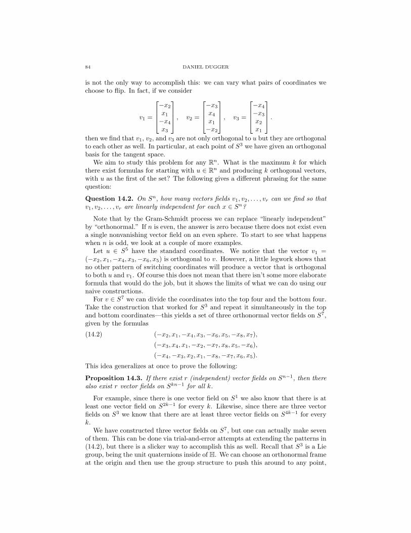
84 DANIEL DUGGER
is not the only way to accomplish this: we can vary what pairs of coordinates wechoose to flip. In fact, if we consider
v1 =
−x2
x1
−x4
x3
, v2 =
−x3
x4
x1
−x2
, v3 =
−x4
−x3
x2
x1
.then we find that v1, v2, and v3 are not only orthogonal to u but they are orthogonalto each other as well. In particular, at each point of S3 we have given an orthogonalbasis for the tangent space.
We aim to study this problem for any Rn. What is the maximum k for whichthere exist formulas for starting with u ∈ Rn and producing k orthogonal vectors,with u as the first of the set? The following gives a different phrasing for the samequestion:
Question 14.2. On Sn, how many vectors fields v1, v2, . . . , vr can we find so thatv1, v2, . . . , vr are linearly independent for each x ∈ Sn?
Note that by the Gram-Schmidt process we can replace “linearly independent”by “orthonormal.” If n is even, the answer is zero because there does not exist evena single nonvanishing vector field on an even sphere. To start to see what happenswhen n is odd, we look at a couple of more examples.
Let u ∈ S5 have the standard coordinates. We notice that the vector v1 =(−x2, x1,−x4, x3,−x6, x5) is orthogonal to v. However, a little legwork shows thatno other pattern of switching coordinates will produce a vector that is orthogonalto both u and v1. Of course this does not mean that there isn’t some more elaborateformula that would do the job, but it shows the limits of what we can do using ournaive constructions.
For v ∈ S7 we can divide the coordinates into the top four and the bottom four.Take the construction that worked for S3 and repeat it simultaneously in the topand bottom coordinates—this yields a set of three orthonormal vector fields on S7,given by the formulas
(−x2, x1,−x4, x3,−x6, x5,−x8, x7),(14.2)
(−x3, x4, x1,−x2,−x7, x8, x5,−x6),
(−x4,−x3, x2, x1,−x8,−x7, x6, x5).
This idea generalizes at once to prove the following:
Proposition 14.3. If there exist r (independent) vector fields on Sn−1, then therealso exist r vector fields on Skn−1 for all k.
For example, since there is one vector field on S1 we also know that there is atleast one vector field on S2k−1 for every k. Likewise, since there are three vectorfields on S3 we know that there are at least three vector fields on S4k−1 for everyk.
We have constructed three vector fields on S7, but one can actually make sevenof them. This can be done via trial-and-error attempts at extending the patterns in(14.2), but there is a slicker way to accomplish this as well. Recall that S3 is a Liegroup, being the unit quaternions inside of H. We can choose an orthonormal frameat the origin and then use the group structure to push this around to any point,
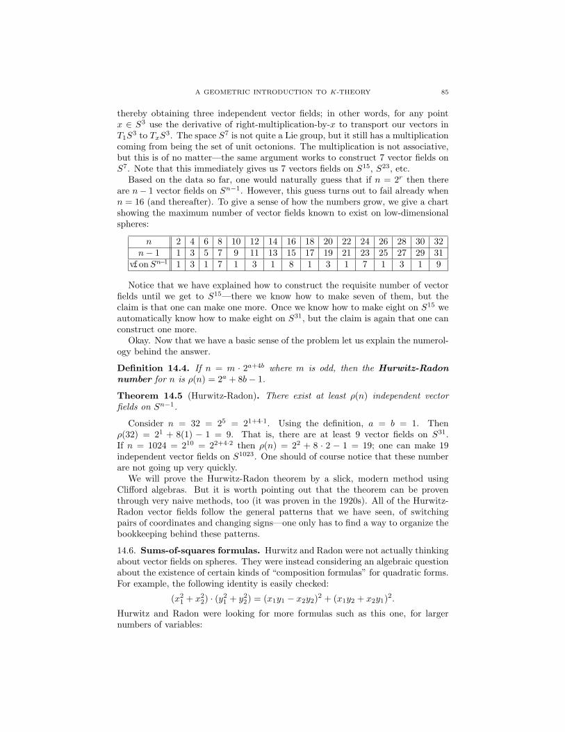
A GEOMETRIC INTRODUCTION TO K-THEORY 85
thereby obtaining three independent vector fields; in other words, for any pointx ∈ S3 use the derivative of right-multiplication-by-x to transport our vectors inT1S
3 to TxS3. The space S7 is not quite a Lie group, but it still has a multiplicationcoming from being the set of unit octonions. The multiplication is not associative,but this is of no matter—the same argument works to construct 7 vector fields onS7. Note that this immediately gives us 7 vectors fields on S15, S23, etc.
Based on the data so far, one would naturally guess that if n = 2r then thereare n− 1 vector fields on Sn−1. However, this guess turns out to fail already whenn = 16 (and thereafter). To give a sense of how the numbers grow, we give a chartshowing the maximum number of vector fields known to exist on low-dimensionalspheres:
n 2 4 6 8 10 12 14 16 18 20 22 24 26 28 30 32n− 1 1 3 5 7 9 11 13 15 17 19 21 23 25 27 29 31
v.f.onSn−1 1 3 1 7 1 3 1 8 1 3 1 7 1 3 1 9
Notice that we have explained how to construct the requisite number of vectorfields until we get to S15—there we know how to make seven of them, but theclaim is that one can make one more. Once we know how to make eight on S15 weautomatically know how to make eight on S31, but the claim is again that one canconstruct one more.
Okay. Now that we have a basic sense of the problem let us explain the numerol-ogy behind the answer.
Definition 14.4. If n = m · 2a+4b where m is odd, then the Hurwitz-Radonnumber for n is ρ(n) = 2a + 8b− 1.
Theorem 14.5 (Hurwitz-Radon). There exist at least ρ(n) independent vectorfields on Sn−1.
Consider n = 32 = 25 = 21+4·1. Using the definition, a = b = 1. Thenρ(32) = 21 + 8(1) − 1 = 9. That is, there are at least 9 vector fields on S31.If n = 1024 = 210 = 22+4·2 then ρ(n) = 22 + 8 · 2 − 1 = 19; one can make 19independent vector fields on S1023. One should of course notice that these numberare not going up very quickly.
We will prove the Hurwitz-Radon theorem by a slick, modern method usingClifford algebras. But it is worth pointing out that the theorem can be proventhrough very naive methods, too (it was proven in the 1920s). All of the Hurwitz-Radon vector fields follow the general patterns that we have seen, of switchingpairs of coordinates and changing signs—one only has to find a way to organize thebookkeeping behind these patterns.
14.6. Sums-of-squares formulas. Hurwitz and Radon were not actually thinkingabout vector fields on spheres. They were instead considering an algebraic questionabout the existence of certain kinds of “composition formulas” for quadratic forms.For example, the following identity is easily checked:
(x21 + x2
2) · (y21 + y2
2) = (x1y1 − x2y2)2 + (x1y2 + x2y1)2.
Hurwitz and Radon were looking for more formulas such as this one, for largernumbers of variables:

86 DANIEL DUGGER
Definition 14.7. A sum-of-squares formulas of type [r, s, n] is an identity
(x21 + x2
2 + . . .+ x2r)(y
21 + y2
2 + . . .+ y2s) = z2
1 + z22 + . . .+ z2
n
in the polynomial ring R[x1, . . . , xr, y1, . . . , ys], where each zi is a bilinear expressionin x’s and y’s.
We will often just refer to an “[r, s, n]-formula”, for brevity. For what values of r,s, and n does such a formula exist? This is currently an open question. There arethree formulas that are easily produced, coming from the normed algebras C, H,and O. The multiplication is a bilinear pairing, and the identity |xy|2 = |x|2|y|2 isthe required sums-of-squares formula. These algebras give formulas of type [2, 2, 2],[4, 4, 4], and [8, 8, 8]. In a theorem from 1898 Hurwitz proved that these are theonly normed algebras over the reals, and in doing so ruled out the existence of[n, n, n]-formulas for n /∈ 1, 2, 4, 8. The question remained (and remains) aboutother types of formulas. See ???? for a detailed history of this problem.
Perhaps surprisingly, most of what is known about the non-existence of sums-of-squares formulas comes from topology. To phrase the question differently, weare looking for a function φ : Rr ⊗ Rs → Rn such that |φ(x, y)|2 = |x|2 · |y|2 for allx ∈ Rr and y ∈ Rs. The bilinear expressions z1, . . . , zn are just the coordinates ofφ(x, y).
Write z = φ(x, y) =∑xjAjy, where the Aj ’s are n × s matrices. The sum of
squares formula says that zT z = (xTx) · (yT y). But zT z =∑i,j
(yTATj xj)(xiAiy),
hence
yT
∑i,j
xixjATj Ai
y = yT((xTx)I
)y
for all y. These quadratic forms in y are equal only if∑i,j
xixjATj Ai = (xTx)I =∑
x2i I, and this must hold for all x. Equating coefficients of the monomials in x,
we find that• ATi Ai = I (that is, Ai ∈ On) for every i, and• ATj Ai +ATi Aj = 0 for every i 6= j.
The case s = n turns out to be significantly simpler to address than the generalcase. If s = n we may set Bi = A−1
i Ai. Then the conditions to satisfy become• BTi = −Bi• B2
i = −In• BiBj = −BjBi for all i 6= j.
Note that the first two conditions imply Bi ∈ On, and the first and third con-ditions imply BTj Bi + BTi Bj = 0. So by replacing the A’s with the B’s we haveproven the following:
Corollary 14.8. If an [r, n, n]-formula exists, then one exists where A1 = I andATi = −Ai.
In the setting of the corollary, the necessary conditions on the matricesA2, A3, . . . , Ar become that A2
i = −I and AiAj = −AjAi.
Corollary 14.9. If an [r, n, n]-formula exists, then there exist r − 1 independentvector fields on Sn−1.
A GEOMETRIC INTRODUCTION TO K-THEORY 87
Proof. If y ∈ Sn−1 then φ(ei, y) ∈ Sn−1 for i = 1, 2, . . . , r: this follows from theidentity |φ(ei, y)|2 = |ei|2 · |y|2. We also have that φ(e1, y) = y since A1 = I. Weclaim that φ(ei, y) ⊥ φ(ej , y) if i 6= j. To see this, note that by the norm formula
|φ(ei + ej , y)|2 = |ei + ej |2 · |y|2 = 2|y|2.On the other hand,
|φ(ei + ej , y)|2 = |φ(ei, y) + φ(ej , y)|2
= |φ(ei, y)|2 + |φ(ej , y)|2 + 2φ(ei, y) · φ(ej , y)
= 2|y|2 + φ(ei, y) · φ(ej , y).
We conclude φ(ei, y) · φ(ej , y) = 0. Therefore we have established that φ(e2,−),φ(e3,−), . . . , φ(er,−) are orthonormal vector fields on Sn−1.
14.10. Clifford algebras. We have seen that we get r − 1 independent vectorfields on Sn−1 if we have a sums-of-squares formula of type [r, n, n]. Having sucha formula amounts to producing matrices A2, A3, . . . , Ar ∈ On such that A2
i = −Iand AiAj + AjAi = 0 for i 6= j. If we disregard the condition that the matricesbe orthogonal, we can encoded the latter two conditions by saying that we have arepresentation of a certain algebra:
Definition 14.11. The Clifford algebra Clk is defined to be the quotient of thetensor algebra R〈e1, . . . , ek〉 by the relations e2i = −1 and eiej + ejei = 0 for alli 6= j.
The first few Clifford algebras are familiar: Cl0 = R, Cl1 = C, and Cl2 = H.After this things become less familiar: for example, it turns out that Cl3 = H×H(we will see why in just a moment). It is somewhat of a miracle that it is possibleto write down a precise description of all of the Clifford algebras, and all of theirmodules. Before doing this, let us be clear about why we are doing it:
Theorem 14.12. An [r, n, n]-formula exists if and only if there exists a Clr−1-module structure on Rn. Consequently, if there is a Clr−1-module structure on Rnthen there are r − 1 independent vector fields on Sn−1.
Before giving the proof, we need one simple fact. The collection of monomialsei1 · · · eir for 1 ≤ i1 < i2 < · · · < ir ≤ k give a vector space basis for Clk, whichhas size 2k (note that we include the empty monomial, corresponding to 1, in thebasis). This is an easy exercise.
Proof of Theorem 14.12. The forward direction is trivial: Given an [r, n, n]-formula, Corollary 14.8 gives us such a formula with A1 = I. Then define a Clr−1-module structure on Rn by letting ei act as multiplication by Ai+1, for 1 ≤ i ≤ r−1.
Conversely, assume that Clr−1 acts on Rn. We can almost reverse the proce-dure of the previous paragraph, except that there is no guarantee that the ei’s actorthogonally on Rn—and we need Ai ∈ On to get an [r, n, n]-formula.
Equip Rn with a positive-definite inner product, denoted x, y 7→ x · y. Thisinner product probably has no compatibility with the Clifford-module structure.So define a new inner product on Rn by
〈v, w〉 =∑
1≤i1<i2<···<ij≤r−1
(eIv) · (eIw),
88 DANIEL DUGGER
where eI = ei1ei2 · · · eij and the sum runs over all 2r−1 elements of the standardbasis for Clr−1. Basically we are averaging out the dot product. Our inner product〈v, w〉 is a symmetric bilinear form, and it is positive definite because the dotproduct is positive definite. It also has the property that it is invariant under theClifford algebra: 〈eiv, eiw〉 = 〈v, w〉 for all i.
Now let v1, . . . , vn be an orthonormal basis for Rn with respect to our new innerproduct. Let Ai be the matrix for ei with respect to this basis. Then the Ai’sare orthogonal matrices, and the relations A2
i = −I and AiAj + AjAi = 0 areautomatic because they are satisfied in Clr−1. In this way we obtain the desired[r, n, n]-formula.
Remark 14.13. Most modern treatments of vector fields on spheres go straightto Clifford algebras and their modules, without ever talking about sums-of-squaresformulas. It seems to us that the sums-of-squares material is an interesting part ofthis whole story, both for historical reasons and for its own sake.
From now on we can focus on the following question: For what values of n do wehave a Clr−1-module structure on Rn? This is the neatest part of the story, becauseon the face of things it doesn’t seem like we have accomplished anything by shiftingour perspective onto Clifford algebras. We have, after all, just rephrased the basicquestion. But a miracle now occurs, in that we can analyze all the Clifford algebrasby a simple trick.
To do this part of the argument, we need a slight variant on our Clifford algebras.Given a real vector space V and a quadratic form q : V → R, define
Cl(V, q) = TR(V )/〈v ⊗ v = q(v) · 1 | v ∈ V 〉.For Rk with q(x1, . . . , xk) = −(x2
1 + · · · + x2k) this recovers the algebra Clk. For
q(x1, . . . , xk) = x21 + · · · + x2
k this gives a new algebra we will call Cl−k . It will beconvenient to temporarily rename Clk as Cl+k . Of course there are other quadraticforms on Rk, but these will be the only two we need for our present purposes.
The discussion that follows is based on the one by Haynes Miller that is givenin [M]. This is by far the best treatment of Clifford algebras that I have found inthe literature.
Proposition 14.14. There are isomorphisms of algebras Cl±k ∼= Cl±2 ⊗R Cl∓k−2.
Proof. One possible isomorphism sends e1 7→ e1 ⊗ 1, e2 7→ e2 ⊗ 1, and for i > 2 wesend ei 7→ e1e2 ⊗ ei−2. We leave it as an exercise to check that this works..
In the analysis that follows we will write A(n) for the algebraMn×n(A), wheneverA is an algebra. The following table gives a list of the first ten Clifford algebras:
We will now explain how to obtain the entries of this table.
Step 1: Rows 0–2.We have already remarked that Cl+0 ∼= R, Cl+1 ∼= C, and Cl+2 ∼= H. It is just as easyto see that Cl−0 ∼= R and Cl−1 ∼= R×R. Finally, with a little more work we also haveCl−2 ∼= R(2). To get this last isomorphism, note that Cl−2 is generated by e1 ande2 subject to the relations e21 = −1, e22 = −1, and e1e2 = −e2e1. The conditionse2i = −1 might make you think of reflections, and we can realize the second relationby using two reflections through lines `1 and `2 of R2 that have a 45 degree angle
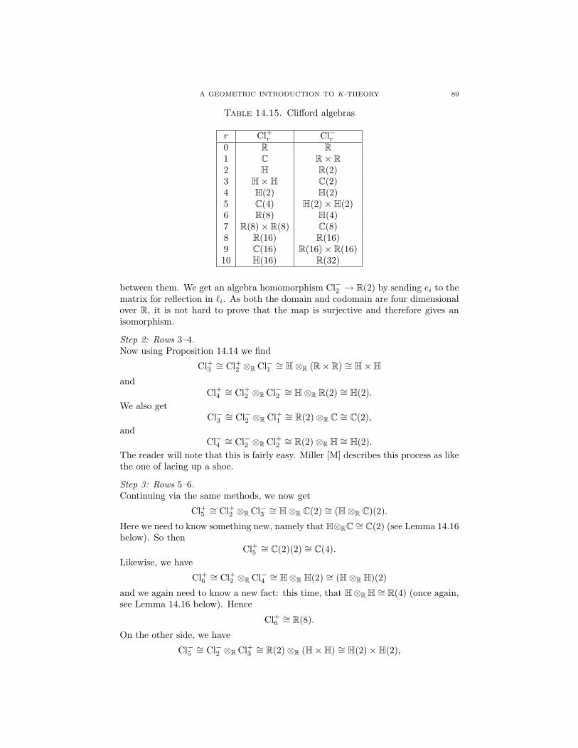
A GEOMETRIC INTRODUCTION TO K-THEORY 89
Table 14.15. Clifford algebras
r Cl+r Cl−r0 R R1 C R× R2 H R(2)3 H×H C(2)4 H(2) H(2)5 C(4) H(2)×H(2)6 R(8) H(4)7 R(8)× R(8) C(8)8 R(16) R(16)9 C(16) R(16)× R(16)10 H(16) R(32)
between them. We get an algebra homomorphism Cl−2 → R(2) by sending ei to thematrix for reflection in `i. As both the domain and codomain are four dimensionalover R, it is not hard to prove that the map is surjective and therefore gives anisomorphism.
Step 2: Rows 3–4.Now using Proposition 14.14 we find
Cl+3 ∼= Cl+2 ⊗R Cl−1 ∼= H⊗R (R× R) ∼= H×Hand
Cl+4 ∼= Cl+2 ⊗R Cl−2 ∼= H⊗R R(2) ∼= H(2).We also get
Cl−3 ∼= Cl−2 ⊗R Cl+1 ∼= R(2)⊗R C ∼= C(2),and
Cl−4 ∼= Cl−2 ⊗R Cl+2 ∼= R(2)⊗R H ∼= H(2).The reader will note that this is fairly easy. Miller [M] describes this process as likethe one of lacing up a shoe.
Step 3: Rows 5–6.Continuing via the same methods, we now get
Cl+5 ∼= Cl+2 ⊗R Cl−3 ∼= H⊗R C(2) ∼= (H⊗R C)(2).
Here we need to know something new, namely that H⊗RC ∼= C(2) (see Lemma 14.16below). So then
Cl+5 ∼= C(2)(2) ∼= C(4).Likewise, we have
Cl+6 ∼= Cl+2 ⊗R Cl−4 ∼= H⊗R H(2) ∼= (H⊗R H)(2)
and we again need to know a new fact: this time, that H⊗R H ∼= R(4) (once again,see Lemma 14.16 below). Hence
Cl+6 ∼= R(8).
On the other side, we have
Cl−5 ∼= Cl−2 ⊗R Cl+3 ∼= R(2)⊗R (H×H) ∼= H(2)×H(2),
90 DANIEL DUGGER
andCl−6 ∼= Cl−2 ⊗R Cl+4 ∼= R(2)⊗R H(2) ∼= H(4).
Step 4: Rows 7–8.Although this may be getting tedious, let’s do it yet again. We have
Cl+7 ∼= Cl+2 ⊗R Cl−5 ∼= H⊗R (H(2)×H(2)) ∼= (H⊗R H)(2)× (H⊗R H)(2)∼= R(8)× R(8),
and
Cl+8 ∼= Cl+2 ⊗R Cl−6 ∼= H⊗R H(4) ∼= (H⊗R H)(4) ∼= R(4)(4) ∼= R(16).
Also,Cl−7 ∼= Cl−2 ⊗R Cl+5 ∼= R(2)⊗R C(4) ∼= C(8)
andCl−8 ∼= Cl−2 ⊗R Cl+6 ∼= R(2)⊗R R(8) ∼= R(16).
Step 5: The rest of the table.We are almost ready to stop. Notice that at row eight the two columns of the tablecome back into juxtaposition: this is a magical fact! We next see that
Cl+9 ∼= Cl+2 ⊗R Cl−7 ∼= H⊗R C(8) ∼= C(16)
andCl+10 ∼= Cl+2 ⊗R Cl−8 ∼= H⊗R R(16) ∼= H(16).
Also,Cl−9 ∼= Cl−2 ⊗R Cl+7 ∼= R(2)⊗R (R(8)× R(8)) ∼= R(16)× R(16)
andCl−10 ∼= Cl−2 ⊗R Cl+8 ∼= R(2)⊗R R(16) ∼= R(32).
It is completely trivial to now prove by induction that
Cl+k+8∼= Cl+k (16) and Cl−k+8
∼= Cl−k (16).
So the table has a quasi-periodicity to it, repeating every eight rows but with anextra factor of (16) everywhere. We have successfully determined all the Cliffordalgebras!
The above analysis used two non-obvious isomorphisms, which we now explainin the following lemma:
Lemma 14.16. There are isomorphisms H⊗R C ∼= C(2) and H⊗R H ∼= R(4).
Proof. Define an algebra map φ : H⊗R C→ EndR(H) by sending q ⊗ z to the mapv 7→ qvz and extending linearly. One readily checks that this is a map of algebras.Notice that the map φ(q ⊗ z) is actually C-linear, if we give H the right action ofC. So we actually have a map of algebras H ⊗R C → EndC(H) ∼= C(2). Both thedomain and targer are four-dimensional over C, and it is not hard to prove thatthe map is surjective—hence, it is an isomorphism.
The proof of the second claim is similar. Define θ : H⊗R H→ EndR(H) ∼= R(4)by sending q ⊗ u to the map v 7→ qvu. The conjugation is needed in order to get amap of algebras. ???

A GEOMETRIC INTRODUCTION TO K-THEORY 91
14.17. Modules over Clifford algebras. Now that we know all the Clifford al-gebras, it is actually an easy process to determine all of their finitely-generatedmodules. We need three facts:
• If A is a division algebra then all modules over A are free;• By Morita theory, the finitely-generated modules over A(n) are in bijective
correspondence with the finitely-generated modules over A. The bijectionsends an A-module M to the A(n)-module Mn.
• If R and S are algebras then modules over R × S can all be written asM ×N where M is an R-module and N is an S-module.
In the following table we list each Clifford algebra Cl+r and the dimension of itssmallest nonzero module.
Table 14.18. Dimensions of Clifford modules
r Cl+r Smallest dim. of a module over Cl+r0 R 11 C 22 H 43 H×H 44 H(2) 85 C(4) 86 R(8) 87 R(8)× R(8) 88 R(16) 169 C(16) 3210 H(16) 64
Note that the third column has a quasi-periodicity, where row k + 8 is obtainedfrom row k by multiplying by 16.
After all of this, we are ready to prove the Hurwitz-Radon theorem about con-structing vector fields on spheres. Recall that if Clr−1 acts on Rn then there arer − 1 independent vector fields on Sn−1. Going down the rows of the above table,we make the following deductions:
Cl1 acts on R2, therefore we have 1 vector field on S1
Cl2 acts on R4, therefore we have 2 vector field on S3
Cl3 acts on R4, therefore we have 3 vector field on S3
Cl4 acts on R8, therefore we have 4 vector field on S7
Cl5 acts on R8, therefore we have 5 vector field on S7
Cl6 acts on R8, therefore we have 6 vector field on S7
Cl7 acts on R8, therefore we have 7 vector field on S7
Cl8 acts on R16, therefore we have 8 vector field on S15.
It is not hard to deduce the general pattern here. The key is knowing where thejumps in dimension occur, and then just doing bookkeeping. To this end, note that
92 DANIEL DUGGER
the smallest dimension of a nonzero module over Clr is 2σ(r) where
σ(r) = #s : 0 < s ≤ r and s ≡ 0, 1, 2, or 4 mod (8)
We know that we can construct r independent vector fields on S2σ(r)−1.
Proof of Theorem 14.5 (Hurwitz-Radon Theorem). First note that we know muchmore about Clifford modules than is indicated in Table 14.18. For each Cliffordalgebra Clr we know the complete list of all isomorphism classes of finitely-generatedmodules, and their dimensions are all multiples of the dimension listed in the table.This is important.
Given an n ≥ 1, our job is to determine the largest r for which Clr acts on Rn.We will then know that there are r vector fields on Sn−1. If we write n = 2u · (odd)it is clear from Table 14.18 and the previous paragraph that the only way Clr couldact on Rn is if it actually acts on R2u
. Moreover, the quasi-periodicity in the tableshows that if we add 4 to u then the largest r goes up by 8. It follows at oncethat if u = a + 4b then the formula for the largest r is 8b+??? where the missingexpression just needs to be something that works for the values a = 0, 1, 2, 3. Onereadily finds that r = 8b+ 2a − 1 does the job.
So we know that there are 8b + 2a − 1 vector fields on Sn−1, where n has theform (odd) · 2a+4b.
Remark 14.19 (First connection with KO∗). Return to Table 14.18 and look atthe column with the smallest dimensions of the modules. As one reads down the col-umn, consider where the jumps in dimensions occur: we have “jump-jump-nothing-jump-nothing-nothing-nothing-jump,” which then repeats. This is strangely remi-niscent of the periodic sequence
Z2 Z2 0 Z 0 0 0 Z . . .This is quite the coincidence, and must have been a source of much excitementwhen it was first noticed. We will eventually see, following [ABS], that there isa very direct connection between the groups KO∗ and the module theory of theClifford algebras. For now we leave it as an intriguing coincidence.
14.20. Adams’s Theorem. So far we have done all this work just to constructcollections of independent vector fields on spheres. The Hurwitz-Radon lower boundis classical, and was probably well-known in the 1940’s. The natural question is,can one do any better? Is there a different construction that would yield morevector fields than we have managed to produce? People were actively working onthis problem throughout the 1950’s. Adams finally proved in 1962 [Ad2] that theHurwitz-Radon bound was maximal, and he did this by using K-theory:
Theorem 14.21 (Adams). There do not exist ρ(n) + 1 independent vector fieldson Sn−1.
This is a difficult theorem, and it will be a long while before we are able to proveit. We are introducing it here largely to whet the reader’s appetite. Note that it isfar from being immediately clear how a cohomology theory would help one provethe result. There are several reductions one must make in the problem, but thefirst one we can explain without much effort:
A GEOMETRIC INTRODUCTION TO K-THEORY 93
Proposition 14.22. If there are r − 1 vector fields on Sn−1 then the projectionRPun−1/RPun−r−1 → RPun−1/RPun−2 ∼= Sun−1 has a section in the homotopycategory, for every u > 2k−2
n .
The existence of a section in the homotopy category is something that can per-haps be contradicted by applying a suitable cohomology theory E∗(−). See Exer-cise 14.24 below for a simple example.
We close this section by sketching the proof of Proposition 14.22. Define
Vk(Rn) = (u1, . . . , uk) |ui ∈ Rn and u1, . . . , uk are orthonormal.This is called the Stiefel manifold of k-frames in Rn. Consider the mapp1 : Vk(Rn) → Sn−1 which sends (u1, . . . , un) 7→ u1. There exist r vector fieldson Sn−1 if and only if there is a section of p1 : Vr+1(Rn)→ Sn−1.
We need a fact from basic topology, namely that there is a cell structure onVk(Rn) where the cells look like
ei1 × · · · × eis
with n− k ≤ i1 < i2 < · · · < is ≤ n− 1 and s is arbitrary. We will not prove thishere: see Hatcher [Ha, Section 3.D] or Mosher-Tangora [MT, ???].
The cell structure looks like[en−k ∪ en−k+1 ∪ · · · ∪ en−1
]∪[(en−k+1 × en−k) ∪ (en−k+2 × en−k) ∪ · · ·
]∪ · · ·
If n− 1 < (n− k+ 1) + (n− k) (these are the dimensions of the last cell in the firstgroup and the first cell in the second group) then the (n− 1)-skeleton just consistsof the cells en−k through en−1. This looks like the top part of the cell structure forRPn−1, and indeed it is:
Proposition 14.23. If n + 2 > 2k then the n-skeleton of our cell structure onVk(Rn) is homeomorphic to RPn−1/RPn−k−1.
Proof. See [MT, ???].
Proof of Proposition 14.22. If there exist r − 1 vector fields on Sn−1 there alsoexist r − 1 vector fields on Sun−1 for any u (see Proposition 14.3). Thenp1 : Vr(Run) → Sun−1 has a section s. By the cellular approximation theorem themap s is homotopic to a cellular map s′. So s′ factors through the (un−1)-skeletonof Vr(Run), which is RPun−1/RPun−r−1 under the assumption that ??????. Wehave
Sun−1 s′−→ RPun−1/RPun−r−1 π−→ RPun−1/RPun−2 ∼= Sun−1.
The composition is p1s′, which is homotopic to p1s = id.
Exercise 14.24. Use singular cohomology to prove that RPn−1/RPn−3 → Sn−1
does not have a section when n is odd. Deduce that an even sphere does not havea non-vanishing vector field (which you already knew).
94 DANIEL DUGGER
Part 3. K-theory and geometry I
At this point we have seen that there exist cohomology theories K∗(−) andKO∗(−). We have not proven their existence, but we have seen that their existencefalls out as a consequence of the Bott periodicity theorems Ω2(Z×BU) ' Z×BUand Ω8(Z× BO) ' Z× BO. If the only cohomology theory you have even seen issingular cohomology, this will seem like an amazing thing: suddenly you know threetimes as many cohomology theories as you used to. But a deeper study reveals thatcohomology theories are actually quite common—to be a little poetic about it, thatthey are as plentiful as grains of sand on the beach. What is rare, however, is tohave cohomology theories with a close connection to geometry: and both K andKO belong to this (vaguely-defined) class. In the following sections we will beginto explore what this means.
To some extent we have a “geometric” understanding of K0(−) and KO0(−) interms of Grothendieck groups of vector bundles. We also know that any Kn(−) (orKOn(−)) group can be shifted to a K0(−) group using the suspension isomorphismand Bott periodicity. One often hears a slogan like “The geometry behind K-theorylies in vector bundles”. This slogan, however, doesn’t really say very much; our aimwill be to do better.
One way to encode geometry into a cohomology theory is via Thom classes forvector bundles. Such classes give rise to fundamental classes for submanifolds anda robust connection wth intersection theory. In the next section we begin our storyby recalling how all of this works for singular cohomology.
15. The Thom isomorphism for singular cohomology
The theory of Thom classes begins with the cohomological approach to orienta-tions. Recall that
H∗(Rn,Rn − 0) ∼= H∗(Dn, Sn−1) ∼= H∗(Sn) ∼=
Z if ∗ = n,
0 otherwise.
Moreover, an orientation on Rn determines a generator for Hn(Rn,Rn − 0) ∼= Z.(For a review of how this correspondence works, see the proof of Lemma 16.2 inthe next section).
Now consider a vector bundle p : E → B of rank n. Let ζ : B → E be the zerosection, and write E−0 as shorthand for E−im(ζ). For any x ∈ B let Fx = p−1(x).Then Hn(Fx, Fx − 0) ∼= Z, and an orientation of the fiber gives a generator. Wewish to consider the problem of giving compatible orientations for all the fibers atonce; this can be addressed through the cohomology of the pair (E,E − 0).
For a neighborhood V of x, let EV = E|V = p−1(V ). If EV is trivial, thenthere is an isomorphism EV ∼= V × Rn, and (EV − 0) ∼= V × (Rn − 0). Hence,H∗(EV , EV − 0) ∼= H∗(V × Rn, V × (Rn − 0)). If V is contractible, this gives that
H∗(EV , EV − 0) ∼= H∗(Rn,Rn − 0) ∼=
Z if ∗ = n,
0 otherwise.
Pick a generator UV ∈ Hn(EV , EV − 0) ∼= Z. For all x ∈ V the inclusionjx : (Fx, Fx−0) → (EV , EV −0) gives a map j∗x : H∗(EV , EV −0)→ H∗(Fx, Fx−0).Since we are assuming that V is contractible, j∗x is an isomorphism. So UV gives
A GEOMETRIC INTRODUCTION TO K-THEORY 95
rise to generators in Hn(Fx, Fx − 0) for all x ∈ V . We think of UV as orienting allof the fibers simultaneously.
Even when V is not contractible the conclusions of the last paragraph still hold.One has that H∗(V ×Rn, V ×(Rn−0)) ∼= H∗(V )⊗H∗(Rn,Rn−0) by the KunnethTheorem, and so
Hi(V × Rn, V × (Rn − 0)) ∼= Hi−n(V )⊗Hn(Rn,Rn − 0) ∼=
Hi−n(V ) if i ≥ n,0 if i < n.
Let UV ∈ Hn(EV , EV −0) be an element that corresponds to 1 ∈ H0(V ) under theabove isomorphism. Then one checks that j∗x(UV ) is a generator for Hn(Fx, Fx−0)for every x ∈ V .
Next suppose that we have two open sets V,W ⊆ B, together with classesUV ∈ Hn(EV , EV − 0) and UW ∈ Hn(EW , EW − 0) that restrict to generators(orientations) on the fibers Fx for every x ∈ V and every x ∈ W , respectively.We would like to require that these orientations match: so we require that theimages of UV and UW in Hn(EV ∩W , EV ∩W − 0) coincide. Consider the (relative)Mayer-Vietoris sequence:
Hn−1(EV ∩W , EV ∩W − 0)
Hn(EV ∩W , EV ∩W − 0)
Hn(EV , EV − 0)⊕Hn(EW , EW − 0)
oo Hn(EV ∪W , EV ∪W − 0)oo
Under our requirement of compatibility between UV and UW , the class UV ⊕ UWmaps to zero; so it is the image of a class UV ∪W . SinceHn−1(EV ∩W , EV ∩W−0) = 0,the class UV ∪W is unique. Note that the Mayer-Vietories sequence also shows thatH∗(EV ∪W , EV ∪W −0) = 0 for ∗ < n, which leaves us poised to inductively continuethis argument. In other words, the argument shows that we may patch more andmore U-classes together, provided that they agree on the regions of overlap. Thisis the kind of behavior one would expect for orientation classes.
The above discussion suggests the following definition:
Definition 15.1. Given a rank n bundle E → B, a Thom class for E is anelement UE ∈ Hn(E,E − 0) such that for all x ∈ B, j∗x(UE) is a generator inHn(Fx, Fx − 0). (Here jx : Fx → E is the inclusion of the fiber).
There is no guarantee that a bundle has a Thom class. Indeed, consider thefollowing example:
Example 15.2. Let M → S1 be the Mobius bundle. Take two contractible opensubsets V and W of S1, where V ∪ W = S1. We can choose a Thom class forM |V , and one for M |W , but the orientations won’t line up correctly to give us aThom class for M . In fact, notice that by homotopy invariance H∗(M,M − 0) isthe cohomology of the Mobius band relative to its boundary. But collapsing theboundary of the band gives an RP 2
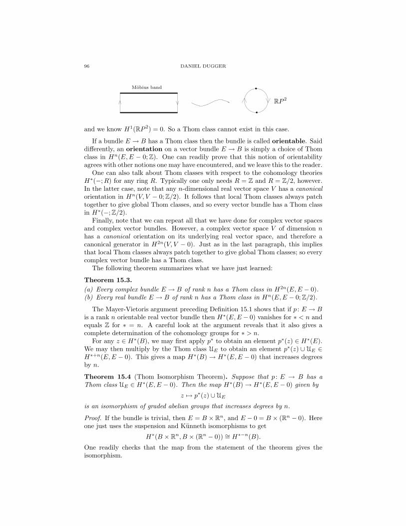
96 DANIEL DUGGER
RP 2
Mobius band
and we know H1(RP 2) = 0. So a Thom class cannot exist in this case.
If a bundle E → B has a Thom class then the bundle is called orientable. Saiddifferently, an orientation on a vector bundle E → B is simply a choice of Thomclass in Hn(E,E − 0; Z). One can readily prove that this notion of orientabilityagrees with other notions one may have encountered, and we leave this to the reader.
One can also talk about Thom classes with respect to the cohomology theoriesH∗(−;R) for any ring R. Typically one only needs R = Z and R = Z/2, however.In the latter case, note that any n-dimensional real vector space V has a canonicalorientation in Hn(V, V − 0; Z/2). It follows that local Thom classes always patchtogether to give global Thom classes, and so every vector bundle has a Thom classin H∗(−; Z/2).
Finally, note that we can repeat all that we have done for complex vector spacesand complex vector bundles. However, a complex vector space V of dimension nhas a canonical orientation on its underlying real vector space, and therefore acanonical generator in H2n(V, V − 0). Just as in the last paragraph, this impliesthat local Thom classes always patch together to give global Thom classes; so everycomplex vector bundle has a Thom class.
The following theorem summarizes what we have just learned:
Theorem 15.3.(a) Every complex bundle E → B of rank n has a Thom class in H2n(E,E − 0).(b) Every real bundle E → B of rank n has a Thom class in Hn(E,E − 0; Z/2).
The Mayer-Vietoris argument preceding Definition 15.1 shows that if p : E → Bis a rank n orientable real vector bundle then H∗(E,E − 0) vanishes for ∗ < n andequals Z for ∗ = n. A careful look at the argument reveals that it also gives acomplete determination of the cohomology groups for ∗ > n.
For any z ∈ H∗(B), we may first apply p∗ to obtain an element p∗(z) ∈ H∗(E).We may then multiply by the Thom class UE to obtain an element p∗(z) ∪ UE ∈H∗+n(E,E − 0). This gives a map H∗(B)→ H∗(E,E − 0) that increases degreesby n.
Theorem 15.4 (Thom Isomorphism Theorem). Suppose that p : E → B has aThom class UE ∈ H∗(E,E − 0). Then the map H∗(B)→ H∗(E,E − 0) given by
z 7→ p∗(z) ∪ UE
is an isomorphism of graded abelian groups that increases degrees by n.
Proof. If the bundle is trivial, then E = B × Rn, and E − 0 = B × (Rn − 0). Hereone just uses the suspension and Kunneth isomorphisms to get
H∗(B × Rn, B × (Rn − 0)) ∼= H∗−n(B).
One readily checks that the map from the statement of the theorem gives theisomorphism.
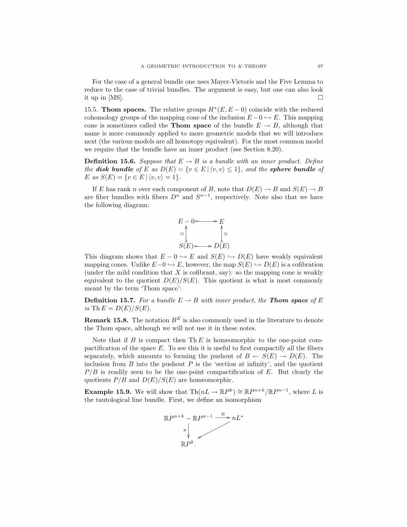
A GEOMETRIC INTRODUCTION TO K-THEORY 97
For the case of a general bundle one uses Mayer-Vietoris and the Five Lemma toreduce to the case of trivial bundles. The argument is easy, but one can also lookit up in [MS].
15.5. Thom spaces. The relative groups H∗(E,E − 0) coincide with the reducedcohomology groups of the mapping cone of the inclusion E−0 → E. This mappingcone is sometimes called the Thom space of the bundle E → B, although thatname is more commonly applied to more geometric models that we will introducenext (the various models are all homotopy equivalent). For the most common modelwe require that the bundle have an inner product (see Section 8.20).
Definition 15.6. Suppose that E → B is a bundle with an inner product. Definethe disk bundle of E as D(E) = v ∈ E | 〈v, v〉 ≤ 1, and the sphere bundle ofE as S(E) = v ∈ E | 〈v, v〉 = 1.
If E has rank n over each component of B, note that D(E)→ B and S(E)→ Bare fiber bundles with fibers Dn and Sn−1, respectively. Note also that we havethe following diagram:
E − 0 // // E
S(E) // //OO
'
OO
D(E)OO'
OO
This diagram shows that E − 0 → E and S(E) → D(E) have weakly equivalentmapping cones. Unlike E−0 → E, however, the map S(E) → D(E) is a cofibration(under the mild condition that X is cofibrant, say): so the mapping cone is weaklyequivalent to the quotient D(E)/S(E). This quotient is what is most commonlymeant by the term ‘Thom space’:
Definition 15.7. For a bundle E → B with inner product, the Thom space of Eis ThE = D(E)/S(E).
Remark 15.8. The notation BE is also commonly used in the literature to denotethe Thom space, although we will not use it in these notes.
Note that if B is compact then ThE is homeomorphic to the one-point com-pactification of the space E. To see this it is useful to first compactify all the fibersseparately, which amounts to forming the pushout of B ← S(E) → D(E). Theinclusion from B into the pushout P is the ‘section at infinity’, and the quotientP/B is readily seen to be the one-point compactification of E. But clearly thequotients P/B and D(E)/S(E) are homeomorphic.
Example 15.9. We will show that Th(nL→ RP k) ∼= RPn+k/RPn−1, where L isthe tautological line bundle. First, we define an isomorphism
RPn+k − RPn−1∼= //
π
nL∗
wwppppppppppp
RP k.
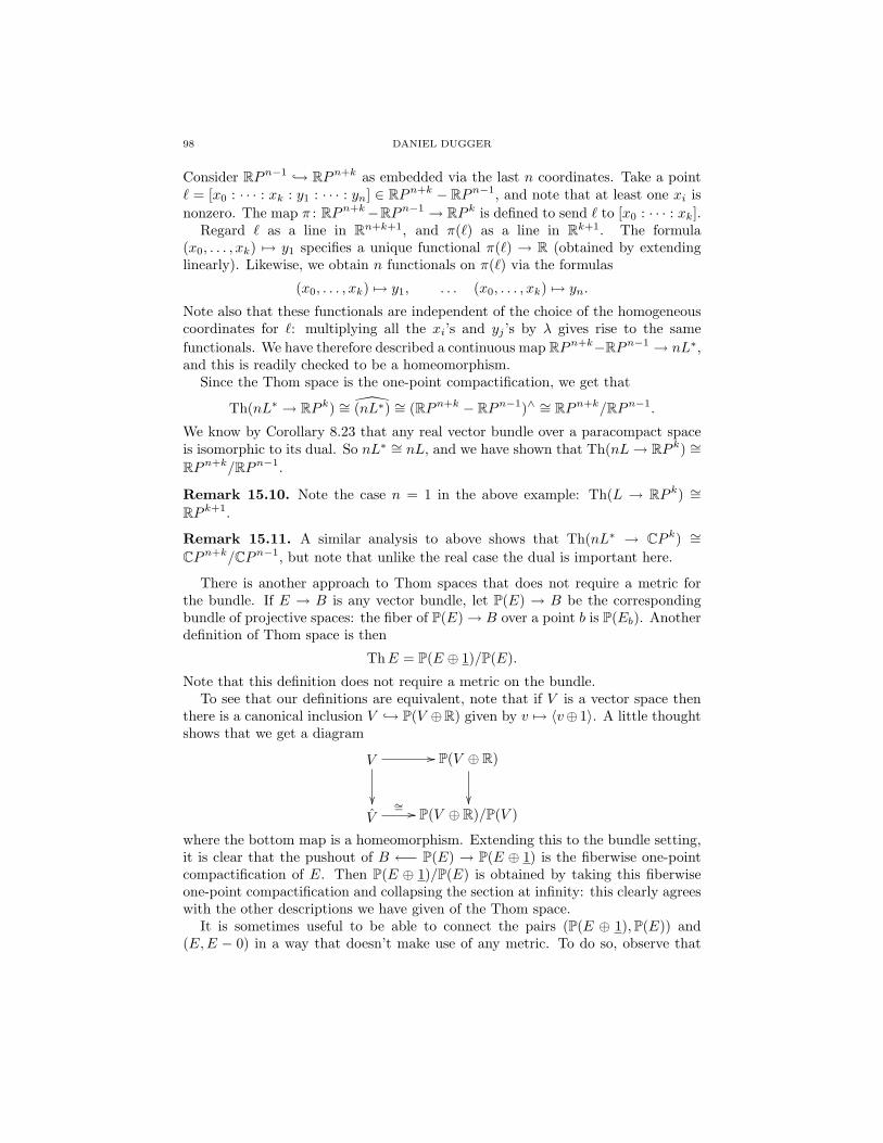
98 DANIEL DUGGER
Consider RPn−1 → RPn+k as embedded via the last n coordinates. Take a point` = [x0 : · · · : xk : y1 : · · · : yn] ∈ RPn+k − RPn−1, and note that at least one xi isnonzero. The map π : RPn+k−RPn−1 → RP k is defined to send ` to [x0 : · · · : xk].
Regard ` as a line in Rn+k+1, and π(`) as a line in Rk+1. The formula(x0, . . . , xk) 7→ y1 specifies a unique functional π(`) → R (obtained by extendinglinearly). Likewise, we obtain n functionals on π(`) via the formulas
(x0, . . . , xk) 7→ y1, . . . (x0, . . . , xk) 7→ yn.
Note also that these functionals are independent of the choice of the homogeneouscoordinates for `: multiplying all the xi’s and yj ’s by λ gives rise to the samefunctionals. We have therefore described a continuous map RPn+k−RPn−1 → nL∗,and this is readily checked to be a homeomorphism.
Since the Thom space is the one-point compactification, we get that
Th(nL∗ → RP k) ∼= (nL∗) ∼= (RPn+k − RPn−1)∧ ∼= RPn+k/RPn−1.
We know by Corollary 8.23 that any real vector bundle over a paracompact spaceis isomorphic to its dual. So nL∗ ∼= nL, and we have shown that Th(nL→ RP k) ∼=RPn+k/RPn−1.
Remark 15.10. Note the case n = 1 in the above example: Th(L → RP k) ∼=RP k+1.
Remark 15.11. A similar analysis to above shows that Th(nL∗ → CP k) ∼=CPn+k/CPn−1, but note that unlike the real case the dual is important here.
There is another approach to Thom spaces that does not require a metric forthe bundle. If E → B is any vector bundle, let P(E) → B be the correspondingbundle of projective spaces: the fiber of P(E)→ B over a point b is P(Eb). Anotherdefinition of Thom space is then
ThE = P(E ⊕ 1)/P(E).
Note that this definition does not require a metric on the bundle.To see that our definitions are equivalent, note that if V is a vector space then
there is a canonical inclusion V → P(V ⊕R) given by v 7→ 〈v⊕ 1〉. A little thoughtshows that we get a diagram
V //
P(V ⊕ R)
V
∼= // P(V ⊕ R)/P(V )
where the bottom map is a homeomorphism. Extending this to the bundle setting,it is clear that the pushout of B ←− P(E) → P(E ⊕ 1) is the fiberwise one-pointcompactification of E. Then P(E ⊕ 1)/P(E) is obtained by taking this fiberwiseone-point compactification and collapsing the section at infinity: this clearly agreeswith the other descriptions we have given of the Thom space.
It is sometimes useful to be able to connect the pairs (P(E ⊕ 1),P(E)) and(E,E − 0) in a way that doesn’t make use of any metric. To do so, observe that

A GEOMETRIC INTRODUCTION TO K-THEORY 99
every vector space V gives rise to a commutative diagram
V − 0
// // P(V ⊕ R)− ∗
P(V )
∼oo
V // // P(V ⊕ R) P(V ⊕ R).
Here ∗ ∈ P(V ⊕R) is the line formed by the distinguished copy of R, and V → P(V ⊕R) is the map v 7→ 〈v ⊕ 1〉; all the other maps are the evident inclusions. Takinghomotopy cofibers of the three columns, one gets a zig-zag of weak equivalencesbetween the homotopy cofiber of V − 0 → V and the homotopy cofiber of P(V ⊕R)/P(V ). The latter is weakly equivalent to its cofiber, because P(V ) → P(V ⊕R)is a cofibration.
Now consider a fiberwise version of the above diagram. If E → B is a real bundlethen we have maps
E − 0
// // P(E ⊕ 1)−B
P(E)
∼oo
E // // P(E ⊕ 1) P(E ⊕ 1).
The only difference worth noting is that B → P(E⊕1) is the evident section that ineach fiber selects out the distinguished line determined by the trivial bundle 1. Theleft square is again a homotopy pushout square, and so taking homotopy cofibersof the columns gives a zig-zag of weak equivalences between the homotopy cofibersof E − 0 → E and P(E) → P(E ⊕ 1).
15.12. Thom spaces for virtual bundles. Thom spaces behave in a very simpleway in relation to adding on trivial bundles:
Proposition 15.13. For any real bundle E → X one has Th(E⊕n) ∼= Σn Th(E).For a complex bundle E → X one has Th(E ⊕ n) ∼= Σ2n Th(E).
Proof. We only prove the statement for real bundles, as the case of complex bundlesworks the same (and is even a consequence of the real case). Also, we will givethe proof assuming the bundle has a metric, although the result is true in moregenerality. Note the isomorphisms
D(E⊕n) ∼= D(E)×Dn, S(E⊕n) ∼= (S(E)×Dn)qS(E)×Sn−1 (D(E)×Sn−1).
From this one readily sees that
D(E ⊕ n)/S(E ⊕ n) ∼= [D(E)/S(E)] ∧ [Dn/Sn−1] ∼= Th(E) ∧ Sn.
Proposition 15.13 allows one to make sense of Thom spaces for virtual bundles,provided that we use spectra. This material will only be needed briefly in the restof the notes, but we include it here because these Thom spectra play a large rolein modern algebraic topology.
Assume that X is compact and let E → X be a bundle. Then E embeds in sometrivial bundle N ; let Q denote the quotient, so that we have E⊕Q ∼= N . Assumingthat Th(−E) had some meaning then we would expect
Th(Q) = Th(N − E) = ΣN Th(−E).
100 DANIEL DUGGER
This suggests the definition
Th(−E) = Σ−N Th(Q),
where the negative suspension must of course be interpreted as taking place in asuitable category of spectra.
Our definition seems to depend on the choice of embedding E → N . To see thatthis dependence is an illusion, let E → N ′ be another embedding and let Q′ bethe quotient. Then N ′ ⊕ Q ∼= Q′ ⊕ E ⊕ Q ∼= Q′ ⊕ N . On Thom spaces this givesΣN
′Th(Q) ∼= ΣN Th(Q′), or Σ−N Th(Q) ' Σ−N
′Th(Q′).
The above discussion can be extended to cover any element α ∈ KO(X). Writeα = E − F for vector bundles E and F , and choose an embedding F → N . LetQ denote the quotient N/F . Note that α +N = (E − F ) + (F +Q) = E +Q. IfTh(α) makes sense then we would expect ΣN (Thα) ' Th(α + N) ' Th(E + Q),and so this suggests the definition
Th(α) = Σ−N Th(E ⊕Q).
Again, one readily checks that this does not depend on the choice of E, F , N , orthe embedding F → N .
15.14. An application to stunted projective spaces. To demonstrate the use-fulness of Thom spaces we give an application to periodicities amongst stuntedprojective spaces. This material will be needed later, in the solution of the vectorfields on spheres problem.
Consider the space RP a+b/RP a. This has a cell structure with exactly b cells(not including the zero cell), in dimensions a + 1 through a + b. The spaceRP a+b+r/RP a+r has a similar cell structure, although here the cells are in di-mensions a+ 1 + r through a+ b+ r. The natural question arises: fixing a and b,what values of r (if any) satisfy
Σr[RP a+b/RP a] ' RP a+b+r/RP a+r.One can use singular cohomology and Steenrod operations to produce some neces-sary conditions here. For example, integral singular homology easily yields that ifif b ≥ 2 then r must be even. Use of Steenrod operations produces more stringentconditions (we leave this for the reader to think about).
We will use Thom spaces to provide some sufficient conditions for a stable ho-motopy equivalence between stunted projective spaces. We begin with a simplelemma:
Lemma 15.15. The element λ = [L] − 1 ∈ KO(RPn) satisfies λ2 = −2λ andλn+1 = 0. Consequently, 2nλ = 0.
Proof. L2 is the trivial bundle, and this immediately yields λ2 = −2λ. The secondstatement follows from the fact that RPn may be covered by n + 1 contractiblesets U0, . . . , Un. (If homogeneous coordinates are used on RPn, one may takeUi to be the open set xi 6= 0). The element λ ∈ KO(RPn, ∗) lifts to a classλi ∈ KO(RPn, Ui), and therefore λn+1 is the image of λ0λ1 · · ·λn under the naturalmap
KO(RPn, U0 ∪ · · · ∪ Un)→ KO(RPn).But since ∪iUi = RPn, the domain of the above map is zero; hence λn+1 = 0.
Finally, since λ2 = −2λ it follows that λe = (−2)e−1λ for all e. In particular,(−2)nλ = λn+1 = 0.
A GEOMETRIC INTRODUCTION TO K-THEORY 101
Proposition 15.16. Let r be any positive integer such that r([L] − 1) = 0 inKO(RP b−1). Then there is a stable homotopy equivalence
Σr[RP a+b/RP a] ' RP a+b+r/RP a+r.
Proof. The assumption that r([L] − 1) = 0 implies that rL ⊕ s ∼= r ⊕ s for somes ≥ 0. We have
RP a+b/RP a ∼= Th
((a+1)L
↓RP b−1
)' Σ−r−s Th
((a+1)L⊕r+s
↓RP b−1
)
' Σ−r−s Th
((a+1+r)L⊕s
↓RP b−1
)
' Σ−r Th
((a+1+r)L
↓RP b−1
)' Σ−r
[RP a+b+r/RP a+r
].
The first and last steps use the identification of stunted projective spaces with acorresponding Thom space—see Example 15.9 for this.
Combining Lemma 15.15 and Proposition 15.16 we see that stunted projectivespaces with b cells have a periodicity of 2b−1:
Σ2b−1[RP a+b/RP a
]' RP a+b+2b−1
/RP a+2b−1.
However, this is not the best result along these lines: we will get a better result byfinding the exact order of [L]− 1 in KO(RP b−1). This was determined by Adams;see Theorem 32.14
16. Thom classes and intersection theory
In this section we will see how Thom classes give rise to fundamental classes forsubmanifolds, and we will develop the connection between products of such classesand intersection theory.
Let E → B be a real vector bundle of rank n. In general, E may not have aThom class; and if it does have a Thom class, it actually has two Thom classes(since Hn(E,E − 0) ∼= Z by the Thom Isomorphism Theorem). The situation isfamiliar, as it matches the usual behavior of orientations. It is, of course, possible—and necessary!—to do geometry in a way that includes keeping track of orientationsand computing signs according to whether orientations match up or not. But it iseasier if we are in a situation where we don’t have to keep track of quite so much,and there are two situations with that property: we can work always with mod 2coefficients, or we can work in the setting of complex geometry. In either case wehave canonical Thom classes all the time. In this section, and for most of the restof these notes, we choose to work in the setting of complex bundles and complexgeometry. But it is important to note that almost everything works verbatim forreal bundles if we use Z/2 coefficients, and that many things can be made to workfor oriented real bundles if one is diligent enough about keeping track of signs.
For a rank n complex bundle E → B we have a canonical Thom class UE ∈H2n(E,E − 0). The following result gives two useful properties:
Proposition 16.1.
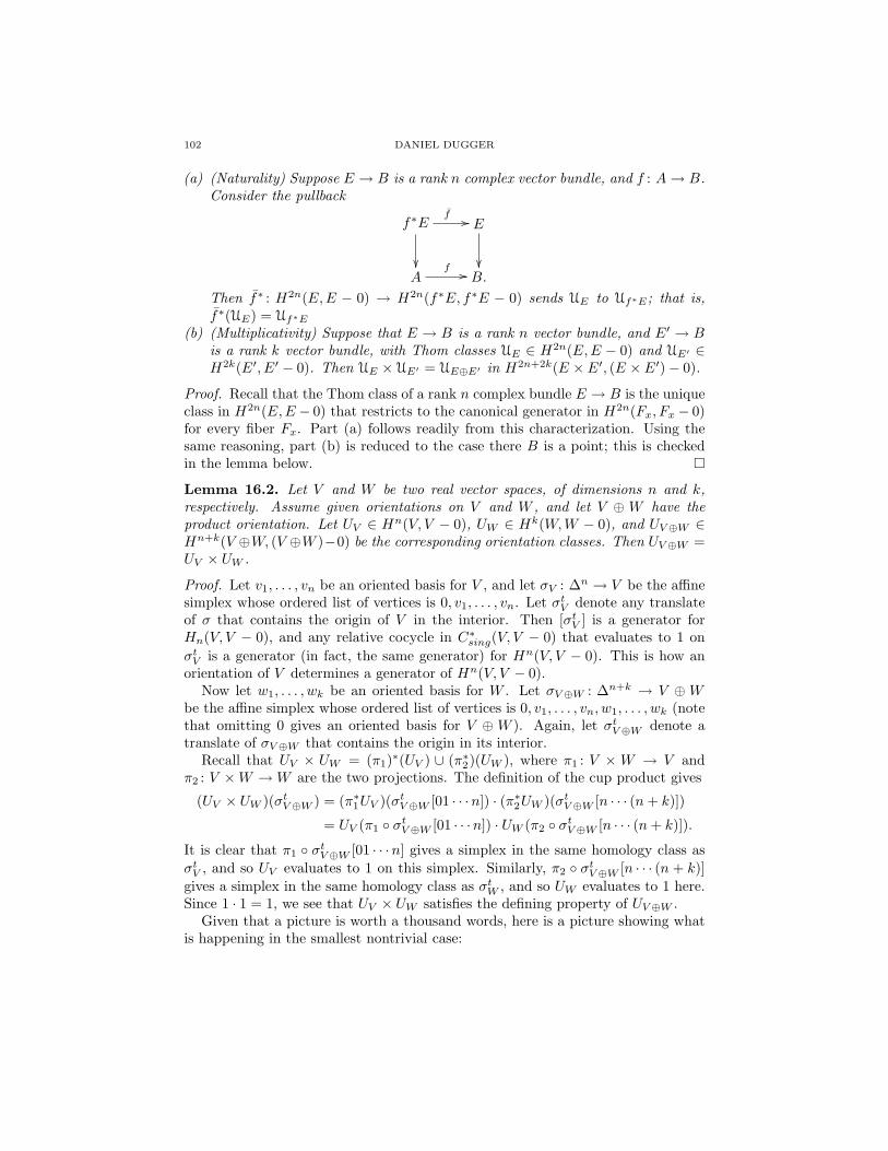
102 DANIEL DUGGER
(a) (Naturality) Suppose E → B is a rank n complex vector bundle, and f : A→ B.Consider the pullback
f∗Ef //
E
A
f // B.
Then f∗ : H2n(E,E − 0) → H2n(f∗E, f∗E − 0) sends UE to Uf∗E; that is,f∗(UE) = Uf∗E
(b) (Multiplicativity) Suppose that E → B is a rank n vector bundle, and E′ → Bis a rank k vector bundle, with Thom classes UE ∈ H2n(E,E − 0) and UE′ ∈H2k(E′, E′ − 0). Then UE × UE′ = UE⊕E′ in H2n+2k(E × E′, (E × E′)− 0).
Proof. Recall that the Thom class of a rank n complex bundle E → B is the uniqueclass in H2n(E,E − 0) that restricts to the canonical generator in H2n(Fx, Fx − 0)for every fiber Fx. Part (a) follows readily from this characterization. Using thesame reasoning, part (b) is reduced to the case there B is a point; this is checkedin the lemma below.
Lemma 16.2. Let V and W be two real vector spaces, of dimensions n and k,respectively. Assume given orientations on V and W , and let V ⊕ W have theproduct orientation. Let UV ∈ Hn(V, V − 0), UW ∈ Hk(W,W − 0), and UV⊕W ∈Hn+k(V ⊕W, (V ⊕W )−0) be the corresponding orientation classes. Then UV⊕W =UV × UW .
Proof. Let v1, . . . , vn be an oriented basis for V , and let σV : ∆n → V be the affinesimplex whose ordered list of vertices is 0, v1, . . . , vn. Let σtV denote any translateof σ that contains the origin of V in the interior. Then [σtV ] is a generator forHn(V, V − 0), and any relative cocycle in C∗sing(V, V − 0) that evaluates to 1 onσtV is a generator (in fact, the same generator) for Hn(V, V − 0). This is how anorientation of V determines a generator of Hn(V, V − 0).
Now let w1, . . . , wk be an oriented basis for W . Let σV⊕W : ∆n+k → V ⊕Wbe the affine simplex whose ordered list of vertices is 0, v1, . . . , vn, w1, . . . , wk (notethat omitting 0 gives an oriented basis for V ⊕ W ). Again, let σtV⊕W denote atranslate of σV⊕W that contains the origin in its interior.
Recall that UV × UW = (π1)∗(UV ) ∪ (π∗2)(UW ), where π1 : V × W → V andπ2 : V ×W →W are the two projections. The definition of the cup product gives
(UV × UW )(σtV⊕W ) = (π∗1UV )(σtV⊕W [01 · · ·n]) · (π∗2UW )(σtV⊕W [n · · · (n+ k)])
= UV (π1 σtV⊕W [01 · · ·n]) · UW (π2 σtV⊕W [n · · · (n+ k)]).
It is clear that π1 σtV⊕W [01 · · ·n] gives a simplex in the same homology class asσtV , and so UV evaluates to 1 on this simplex. Similarly, π2 σtV⊕W [n · · · (n + k)]gives a simplex in the same homology class as σtW , and so UW evaluates to 1 here.Since 1 · 1 = 1, we see that UV × UW satisfies the defining property of UV⊕W .
Given that a picture is worth a thousand words, here is a picture showing whatis happening in the smallest nontrivial case:
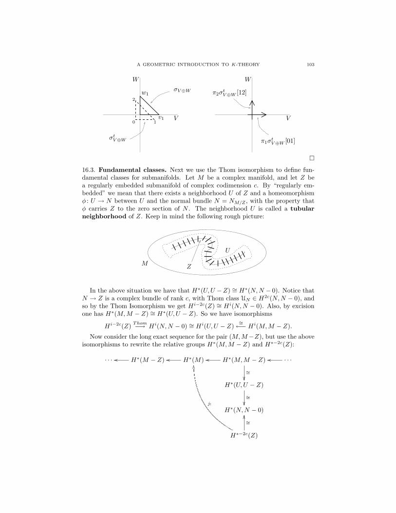
A GEOMETRIC INTRODUCTION TO K-THEORY 103
v1
w1
V V
W W
σV⊕W
σtV⊕W π1σtV⊕W [01]
π2σtV⊕W [12]
0 1
2
16.3. Fundamental classes. Next we use the Thom isomorphism to define fun-damental classes for submanifolds. Let M be a complex manifold, and let Z bea regularly embedded submanifold of complex codimension c. By “regularly em-bedded” we mean that there exists a neighborhood U of Z and a homeomorphismφ : U → N between U and the normal bundle N = NM/Z , with the property thatφ carries Z to the zero section of N . The neighborhood U is called a tubularneighborhood of Z. Keep in mind the following rough picture:
M Z
U
In the above situation we have that H∗(U,U −Z) ∼= H∗(N,N − 0). Notice thatN → Z is a complex bundle of rank c, with Thom class UN ∈ H2c(N,N − 0), andso by the Thom Isomorphism we get Hi−2c(Z) ∼= Hi(N,N − 0). Also, by excisionone has H∗(M,M − Z) ∼= H∗(U,U − Z). So we have isomorphisms
Hi−2c(Z) Thom−→ Hi(N,N − 0) ∼= Hi(U,U − Z)∼=←− Hi(M,M − Z).
Now consider the long exact sequence for the pair (M,M−Z), but use the aboveisomorphisms to rewrite the relative groups H∗(M,M − Z) and H∗−2c(Z):
· · · H∗(M − Z)oo H∗(M)oo H∗(M,M − Z)oo
∼=
· · ·oo
H∗(U,U − Z)
∼=
H∗(N,N − 0)
H∗−2c(Z)
∼=
OO
j!
PP
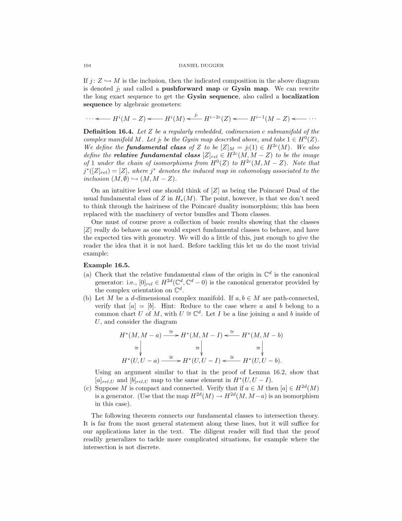
104 DANIEL DUGGER
If j : Z →M is the inclusion, then the indicated composition in the above diagramis denoted j! and called a pushforward map or Gysin map. We can rewritethe long exact sequence to get the Gysin sequence, also called a localizationsequence by algebraic geometers:
· · · Hi(M − Z)oo Hi(M)oo Hi−2c(Z)j!oo Hi−1(M − Z)oo · · ·oo
Definition 16.4. Let Z be a regularly embedded, codimension c submanifold of thecomplex manifold M . Let j! be the Gysin map described above, and take 1 ∈ H0(Z).We define the fundamental class of Z to be [Z]M = j!(1) ∈ H2c(M). We alsodefine the relative fundamental class [Z]rel ∈ H2c(M,M − Z) to be the imageof 1 under the chain of isomorphisms from H0(Z) to H2c(M,M − Z). Note thatj∗([Z]rel) = [Z], where j∗ denotes the induced map in cohomology associated to theinclusion (M, ∅) → (M,M − Z).
On an intuitive level one should think of [Z] as being the Poincare Dual of theusual fundamental class of Z in H∗(M). The point, however, is that we don’t needto think through the hairiness of the Poincare duality isomorphism; this has beenreplaced with the machinery of vector bundles and Thom classes.
One must of course prove a collection of basic results showing that the classes[Z] really do behave as one would expect fundamental classes to behave, and havethe expected ties with geometry. We will do a little of this, just enough to give thereader the idea that it is not hard. Before tackling this let us do the most trivialexample:
Example 16.5.(a) Check that the relative fundamental class of the origin in Cd is the canonical
generator: i.e., [0]rel ∈ H2d(Cd,Cd − 0) is the canonical generator provided bythe complex orientation on Cd.
(b) Let M be a d-dimensional complex manifold. If a, b ∈ M are path-connected,verify that [a] = [b]. Hint: Reduce to the case where a and b belong to acommon chart U of M , with U ∼= Cd. Let I be a line joining a and b inside ofU , and consider the diagram
H∗(M,M − a)
∼=
∼= // H∗(M,M − I)
∼=
H∗(M,M − b)
∼=
∼=oo
H∗(U,U − a)∼= // H∗(U,U − I) H∗(U,U − b).
∼=oo
Using an argument similar to that in the proof of Lemma 16.2, show that[a]rel,U and [b]rel,U map to the same element in H∗(U,U − I).
(c) Suppose M is compact and connected. Verify that if a ∈M then [a] ∈ H2d(M)is a generator. (Use that the mapH2d(M)→ H2d(M,M−a) is an isomorphismin this case).
The following theorem connects our fundamental classes to intersection theory.It is far from the most general statement along these lines, but it will suffice forour applications later in the text. The diligent reader will find that the proofreadily generalizes to tackle more complicated situations, for example where theintersection is not discrete.
A GEOMETRIC INTRODUCTION TO K-THEORY 105
Theorem 16.6. Let M be a connected complex manifold. Suppose that Z and Ware regularly embedded submanifolds of M that intersect transversally in d points.Then(a) [Z]M ∪ [W ]M = d[∗]M(b) j∗([Z]M ) = d[∗]W , where j : W →M .
Proof. We begin by proving (a). Suppose that dimZ = k and dimW = `, so thatdimM = k + `. Let Z ∩W = p1, . . . , pd, and for each i let Ui be a Euclideanneighborhood of pi such that Ui∩Uj = ∅ for i 6= j. Consider the following diagram:
Hk(M,M − Z)⊗H l(M,M −W ) //
∪rel
Hk(M)⊗H l(M)
∪
Hk+l(M,M − (Z ∩W )) // Hk+l(M)
Hk+l(M,M − p1, . . . , pd)
⊕rHk+l(M,M − pr)
∼=
OO
88qqqqqqqqqqqqqqqqqqqqqqqqqq
Since [Z] and [W ] lift to relative classes [Z]rel and [W ]rel, it will suffice to show thatif we take [Z]rel∪[W ]rel and take its projection to the rth factor Hk+l(M,M−pr)of the summand then we get [pr]rel. From this it will follow from the diagram that[Z]∪ [W ] = [p1]+ . . .+[pd] in Hk+l(M). Since we have already seen in Exercise 16.5that [pi] = [pj ] for any i and j, this will complete the proof of (a).
Next, fix an index r and consider the second diagram
Hk(Ur, Ur − Z)⊗H l(Ur, Ur −W )
Hk(M,M − Z)⊗H l(M,M −W )
oo
Hk+l(Ur, Ur − pr) Hk+l(M,M − p1, . . . , pd)oo
Hk+l(M,M − pr).
OO∼=
kkXXXXXXXXXXXXXXXXXXXXX
Thanks to this diagram, it is enough to replace M by Ur, Z by Z ∩ Ur, and W byW ∩ Ur, and to prove that [Z]rel ∪ [W ]rel = [pr]rel.
But now M is just Ck+l. By choosing our neighborhood small enough, we canfind local coordinates so that Z is just Ck andW is just Cl, intersecting transversallyat the origin. We need to compute [Ck]rel ∪ [Cl]rel ∈ Hk+l(Ck+l,Ck+l − 0). Bywriting Ck+l = Ck × Cl one sees that [Ck]rel coincides with the Thom class forthe bundle l → Ck. Likewise, [Cl]rel coincides with the Thom class for the bundlek → Cl. These are trivial bundles, so they are pulled back from Cl → ∗ andCk → ∗ along the projection maps Ck → ∗ and Cl → ∗, respectively. In particular,by Proposition 16.1(a) we can write
[Ck]rel ∪ [Cl]rel = π∗1(U1) ∪ π∗2(U2)
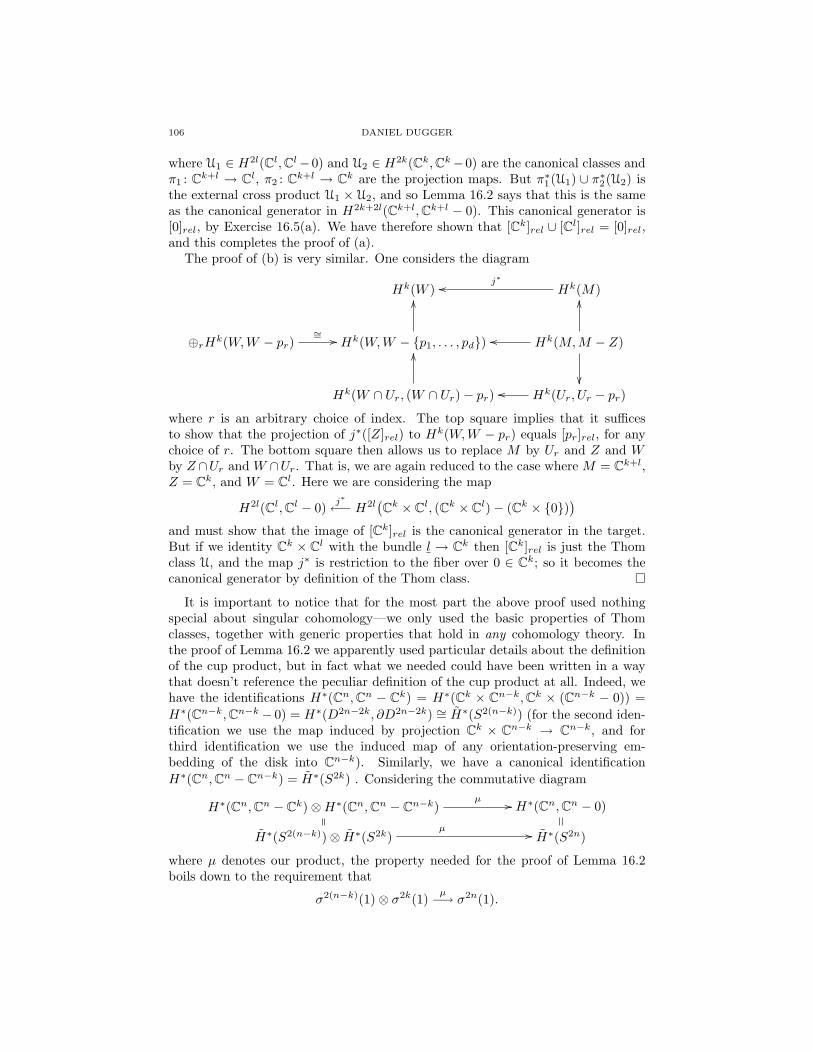
106 DANIEL DUGGER
where U1 ∈ H2l(Cl,Cl−0) and U2 ∈ H2k(Ck,Ck−0) are the canonical classes andπ1 : Ck+l → Cl, π2 : Ck+l → Ck are the projection maps. But π∗1(U1) ∪ π∗2(U2) isthe external cross product U1 × U2, and so Lemma 16.2 says that this is the sameas the canonical generator in H2k+2l(Ck+l,Ck+l − 0). This canonical generator is[0]rel, by Exercise 16.5(a). We have therefore shown that [Ck]rel ∪ [Cl]rel = [0]rel,and this completes the proof of (a).
The proof of (b) is very similar. One considers the diagram
Hk(W ) Hk(M)j∗oo
⊕rHk(W,W − pr)∼= // Hk(W,W − p1, . . . , pd)
OO
Hk(M,M − Z)oo
OO
Hk(W ∩ Ur, (W ∩ Ur)− pr)
OO
Hk(Ur, Ur − pr)oo
where r is an arbitrary choice of index. The top square implies that it sufficesto show that the projection of j∗([Z]rel) to Hk(W,W − pr) equals [pr]rel, for anychoice of r. The bottom square then allows us to replace M by Ur and Z and Wby Z ∩Ur and W ∩Ur. That is, we are again reduced to the case where M = Ck+l,Z = Ck, and W = Cl. Here we are considering the map
H2l(Cl,Cl − 0)j∗←− H2l
(Ck × Cl, (Ck × Cl)− (Ck × 0)
)and must show that the image of [Ck]rel is the canonical generator in the target.But if we identity Ck × Cl with the bundle l → Ck then [Ck]rel is just the Thomclass U, and the map j∗ is restriction to the fiber over 0 ∈ Ck; so it becomes thecanonical generator by definition of the Thom class.
It is important to notice that for the most part the above proof used nothingspecial about singular cohomology—we only used the basic properties of Thomclasses, together with generic properties that hold in any cohomology theory. Inthe proof of Lemma 16.2 we apparently used particular details about the definitionof the cup product, but in fact what we needed could have been written in a waythat doesn’t reference the peculiar definition of the cup product at all. Indeed, wehave the identifications H∗(Cn,Cn − Ck) = H∗(Ck × Cn−k,Ck × (Cn−k − 0)) =H∗(Cn−k,Cn−k − 0) = H∗(D2n−2k, ∂D2n−2k) ∼= H∗(S2(n−k)) (for the second iden-tification we use the map induced by projection Ck × Cn−k → Cn−k, and forthird identification we use the induced map of any orientation-preserving em-bedding of the disk into Cn−k). Similarly, we have a canonical identificationH∗(Cn,Cn − Cn−k) = H∗(S2k) . Considering the commutative diagram
H∗(Cn,Cn − Ck)⊗H∗(Cn,Cn − Cn−k)µ // H∗(Cn,Cn − 0)
H∗(S2(n−k))⊗ H∗(S2k)µ // H∗(S2n)
where µ denotes our product, the property needed for the proof of Lemma 16.2boils down to the requirement that
σ2(n−k)(1)⊗ σ2k(1)µ−→ σ2n(1).

A GEOMETRIC INTRODUCTION TO K-THEORY 107
In other words, the computation comes down to the fact that the product behaveswell with respect to the suspension isomorphism.
Example 16.7. We will be content with the usual first example. Let Z → CPnbe a codimension c complex submanifold. Then [Z] ∈ H2c(CPn) ∼= Z. A generatorfor this group is [CPn−c], so [Z] = d[CPn−c] for a unique integer d. This integer iscalled the degree of the submanifold Z. A generic, c-dimensional, linear subspaceof CPn will intersect Z transversally in finitely many points, say e of them. The-orem 16.6 gives that [Z] ∪ [CP c] = e[∗], but we also have d[CPn−c] ∪ [CP c] = d[∗]since [CPn−c] ∪ [CP c] = [∗] (again by Theorem 16.6). So d = e, and this givesthe geometric description of the degree: the number of intersection points with ageneric linear subpace of complementary dimension.
The following result is the evident generalization of Theorem 16.6.
Theorem 16.8. Let M be a connected complex manifold. Suppose that Z and Ware regularly embedded submanifolds of M that intersect transversally. Then(a) [Z]M ∪ [W ]M = [Z ∩W ];(b) j∗([Z]M ) = [Z ∩W ], where j : W →M .
Outline of proof. We omit the details here, since the proof is largely similar to thatof Theorem 16.6. For (a) use the relative fundamental classes [Z]rel and [W ]rel,and show that [Z]rel ∪ [W ]rel = [Z ∩ W ]rel in H∗(M,M − (Z ∩ W )). For this,restrict to a tubular neighborhood and then show that both classes restrict to thecanonical generators on the fibers of the normal bundle. For [Z ∩W ]rel this is thedefinition, and for [Z]rel ∪ [W ]rel this is a computation with the cup product. Theproof of (b) is similar.
16.9. Topological intersection multiplicities. We can now use our machineryto give a topological definition of intersection multiplicity. Suppose that Z and Ware complex submanifolds of the complex manifold M , and that Z and W have anisolated point of intersection at p. Let U be a Euclidean neighborhood of p thatcontains no other points of Z ∩W . Consider the classes ????
17. Thom classes in K-theory
In the last section we saw how Thom classes for complex vector bundles giverise to cohomological fundamental classes for submanifolds, and we saw that thesefundamental classes have the expected connections to geometry. The discussion wascarried out in the case of singular cohomology, but very little specific informationabout this cohomology theory was actually used. In fact, once we showed thatThom classes existed everything else followed formally. So let us now generalize abit:
Definition 17.1. A multiplicative generalized cohomology theory is a coho-mology theory E equipped with product maps
Ep(X,A)⊗ Eq(Y,B)→ Ep+q(X × Y,X ×B ∪A× Y )
has requirements:(1) natural(2) ∃ unit in E0(pt, ∅) = E0(pt)(3) associative
108 DANIEL DUGGER
(4) compatibility with δ, the connecting homomorphism
Let E be a multiplicative generalized cohomology theory.
Definition 17.2. Let E → B be a rank n complex vector bundle. A Thomclass for E is an element UE ∈ E2n(E,E − 0) such that ∀x ∈ B, i∗(UE) ∈E2n(Fx, Fx \0) ∼= E2n(Cn,Cn \0) ∼= E2n(D2n, ∂D2n) ∼= ˜E2n ∼= E0(S0) = E0(pt), andthe condition is i∗(UE) maps to 1 ∈ E0(pt)
Definition 17.3. A complex orientation for E is a choice, for every rank ncomplex bundle E → B, of a Thom class UE ∈ E2n(E,E − 0) such that
(1) (Naturality) Uf∗E = f∗(UE) for every map f : A→ B;(2) (Multiplicativity) UE⊕E′ = UE · UE′
A given cohomology theory may or may not admit a complex orientation—most likely, it will not. The complex-orientable cohomology theories are a veryspecial class. Note that once a complex orientation is provided one gets the Thomisomorphism, Gysin sequences, and fundamental classes for complex submanifoldsjust as before—as well as the same connections to intersection theory.
Our goal in this section is the following:
Theorem 17.4. Complex K-theory admits a complex orientation.
We will spend a long time exploring the geometric consequences of this, but let usgo ahead and give one example right away. Let Z → CPn be a complex submanifoldof codimension c. The above theorem implies that we have a fundamental class [Z] ∈K2c(CPn), just as we did in the case of singular cohomology. Whereas H2c(CPn) ∼=Z and only resulted in one integral invariant, we will find that K2c(CPn) ∼= Zn+1.This is a much larger group, and so there is suddenly the potential for detectingmore information: the K-theoretic fundamental class [Z] is an (n + 1)-tuple ofintegers rather than just a single integer. Of course it might end up that all of thesenew invariants are just zero, or some algebraic function of the invariant we alreadyhad—we will have to do some computations to find out. But this demonstratesthe general situation: K-theory has an inherent ability to detect more informationthan singular cohomology did.
To prove Theorem 17.4 we need to give a construction, for every rank n complexvector bundle E → B, of a Thom class in K2n(E,E − 0). By Bott periodicity thisgroup is the same as K0(E,E − 0). Our first step will be to develop some tools forproducing elements in relative K-groups.
17.5. Relative K-theory. Let A → X be an inclusion of topological spaces.When we talked about algebraic K-theory back in Part 1, we defined the relativeK-group K0(X,A) using quasi-isomorphism classes of chain complexes that wereexact on A (Section 5.10). We will make a similar construction in the topologicalcase, with some important differences.
Definition 17.6. Let F(X,A) be the free abelian group on isomorphism classes ofbounded chain complexes of vector bundles E• on X that are exact on A (meaningthat for every x ∈ X the complex of vector spaces (Ex)• is exact). Define K(X,A)to be the quotient of F(X,A) by the following relations:(1) [E• ⊕ F•] = [E•] + [F•];(2) [E•] = 0 whenever E• is exact on all of X;

A GEOMETRIC INTRODUCTION TO K-THEORY 109
(3) If E• is a boundex complex of vector bundles on X × I that is exact on A × Ithen [E|X×0] = [E|X×1].
Note that pullback of vector bundles makes K(X,A) into a contravariant functor.Relations (1) and (2) are familiar, although the reader might be surprised that
(1) only deals with direct sums and not short exact sequences. We will say moreabout this in a moment. Let us first make some remarks on relation (3), since wehave not dealt with relations of this type before.
If d : E → F is a map of vector bundles over X there is a clear, intuitive notionof deformation of d. One way to make this rigorous is to consider the subspaceVB(E,F ) ⊆ Top(E,F ) consisting of the vector bundle maps; then a deformation ofd is just a continuous map I → VB(E,F ) that sends 0 to d. If π : X×I → X is theprojection, a little thought shows that the above notion of deformation is the sameas a map of vector bundles π∗E → π∗F over X × I that restricts to d on X × 0.
Likewise, a deformation of a chain complex E• over X can be thought of in twoways. One way involves a collection of deformations for all the maps of E•, havingthe property that at any given time t the maps in the deformation assemble into achain complex. The other way is simply as a chain complex structure on the set ofvector bundles π∗Ei. These notions are equivalent.
The point here is that if (E•, d) is a given chain complex and d′ is a deformationof the differential on d, then relation (3) implies that [(E•, d)] = [(E•, d
′)]. (To beprecise, there is an exactness condition required for the deformation, namely thatat every time t the differential dt is exact on A). Moreover, if X is paracompactHausdorff then by Corollary 11.2(b) every bundle on X × I is isomorphic to thepullback of a bundle from X; it follows that every relation from (3) can be recastin this form. That is to say, for paracompact Hausdorff spaces it is equivalent toreplace (3) by(3’) [(E•, d)] = [(E•, d
′)] for any bounded chain complex (E•, d) and any deforma-tion d′ of d.
The following important lemma will help give a feel for the idea of deforming achain complex:
Lemma 17.7. Let E• be a bounded complex of vector bundles on X that is exacton A. Then [E•] = −[ΣE•] in K(X,A), where ΣE• is the shifted complex havingEi in degree i+ 1.
Proof. First note that if V• and W• are exact complexes of vector spaces andf : V• → W• is any map, then the mapping cone Cf is still exact. This followsby the long exact sequence on homology. Consequently, if E• → F• is a map be-tween complexes of vector bundles on X, each of which is exact on A, then themapping cone is also exact on A.
Let C denote the mapping cone of the identity id : E• → E•. We depict thiscomplex as follows:
· · · // E3
⊕
// E2
⊕
// E1
⊕
// E0
· · ·
>>|||||||| // E2//
id|||
>>|||
E1//
id|||
>>|||
E0
id|||
>>|||
110 DANIEL DUGGER
The arrows depict the various components of the differentials in the mapping cone;recall that d(a, b) = (da+id(b),−db) for (a, b) ∈ En⊕En−1, where we have writtenid(b) just to indicate the role of the original chain map.
Consider the deformation of C obtained by putting a t in front of all the diagonalarrows and letting t 7→ 0. That is, Ct is the mapping cone for t(id) : E• → E•.Then Ct is exact on A for every t, and when t = 0 we have C0 = E• ⊕ ΣE•. So[C] = [C1] = [C0] = [E•] + [ΣE•] in K(X,A).
But C is exact on all of X, being the mapping cone of an identity map. So[C] = 0 in K(X,A), and hence [E•] = −[ΣE•].
Remark 17.8. The ideas used in the above proof immediately also give the fol-lowing. Let E• and F• be complexes of vector bundles on X that are exact onA and let f : E• → F• be any map, with Cf denoting the mapping cone. Then[Cf ] = [F•]− [E•] in K(X,A).
Our next task is to analyze exact complexes, and see that just as in homologicalalgebra they split up into basic pieces.
Definition 17.9. An elementary complex is one of the form
[0→ · · · → 0→ Eid−→ E → 0→ · · · → 0]
where E is a vector bundle on X and the E’s occur in some dimensions i and i+1.Denote this complex as Di(E).
Proposition 17.10. Let X be a paracompact Hausdorff space. If E• is a boundedcomplex of vector bundles on X that is exact, then E• is a direct sum of elementarycomplexes.
Proof. The proof is really the same as in homological algebra. Assume withoutloss of generality that Ei = 0 for i < 0. Then E1 → E0 is a surjection, so thekernel K1 is a vector bundle by Proposition 9.3. By Proposition 9.2 the sequence0→ K1 → E1 → E0 → 0 is split-exact, and a choice of splitting allows us to writeE1∼= K1 ⊕ Q1 where the composite Q1 → E1 → E0 is an isomorphism. Noting
that E2 → E1 has image contained in K1, the complex E• splits as the direct sumof D0(E0) and a complex that is zero in dimensions smaller than 1. Now continueinductively, replacing E• with this smaller factor, until the nonzero degrees of E•
have been exhausted.
Remark 17.11. Observe now that relation (2) of Definition 17.6 could be replacedwith the relation that [Di(E)] = 0 for any vector bundle E on X and any i ∈ Z.This fact is sometimes useful.
The next result explains why we were able to forego short exact sequences inrelation (1) from Definition 17.6.
Proposition 17.12. Let X be paracompact and Hausdorff. Assume given a shortexact sequence 0→ E′• → E• → E′′• → 0 of complexes of vector bundles, where eachcomplex is exact on A. Then [E•] = [E′•] + [E′′• ] in K(X,A).
Proof. Let C• be the mapping cone of E′• → E•, and recall that there is a naturalmap C• E′′• . Let K• be the kernel, which is a chain complex of vector bundlesby Proposition 9.3. Elementary homological algebra (applied in each fiber) showsthat K• is exact on X. By Lemma 17.13 below the inclusion K• → C• is split, and

A GEOMETRIC INTRODUCTION TO K-THEORY 111
so C•∼= K•⊕E′′• . So [C•] = [K•] + [E′′• ] = [E′′• ] in K(X,A). Yet Remark 17.8 gives
[C•] = [E•]− [E′•].
Lemma 17.13. Let X be a paracompact Hausdorff space. Let j : K• → C• be aninclusion between bounded complexes of vector bundles on X, and assume that K•
is exact. Then the map j admits a splitting χ : C• → K•.
Proof. Without loss of generality assume that Ki = 0 = Ci for i < 0. We start bywriting K = ⊕Ni=0D(Ai) for some vector bundles A1, . . . , AN on X. The inclusionj looks as follows:
...id
...
A2 ⊕ A1
id
// C2
A1 ⊕ A0
id
// C1
A0
// C0
Starting at the bottom, choose a splitting χ0 for the inclusion A0 → C0, usingCorollary 9.4. Likewise, choose a splitting α1 for the inclusions A1 → C1/A0 (notethat C1/A0 is a vector bundle by Proposition 9.3). Define χ1 : C1 → A1⊕A0 to bethe sum of C1 → C1/A0
α1−→ A1 and C1 → C0χ0−→ A0. It is readily checked that
χ1 is a splitting for j1 and that dχ1 = χ0d. Continue inductively to define χ at alllevels.
The groups K(X,A) are readily seen to be homotopy invariant constructions:
Proposition 17.14. For any pair (X,A) the map π∗ : K(X,A)→ K(X×I,A×I)is an isomorphism.
Proof. If j0, j1 : (X,A) → (X × I, A× I) are the evident inclusions then it is clearthat j∗0 = j∗1 . It then follows by category theory that homotopic maps (X,A) →(Y,B) induce the same map upon applying K(−,−). Consequently, if f : (X,A)→(Y,B) is part of a relative homotopy equivalence then it induces an isomorphismon K-groups. Now just apply this to π.
Before finishing with our basic exploration of the group K(X,A), let us note thefollowing simple result:
Proposition 17.15. For any compact Hausdorff space X there is an isomorphismK(X, ∅)→ K0(X) given by the formula [E•]→
∑i(−1)i[Ei].
Proof. It is immediate that the indicated formula gives a group homomorphismχ : K(X, ∅) → K0(X); the only nontrivial part is verifying relation (3), but hereone uses that if F is a vector bundle on X × I then F |X×0
∼= F |X×1.There is also the evident map j : K0(X) → K(X, ∅) sending a vector bundle E
to the chain complex E[0] consisting of E in degree 0 and zeros in all other degrees.Certainly χ j = id.
If E• is any chain complex of vector bundles on X then we may deform E• tothe complex with zero differentials, by putting a t in front of all the d maps andletting t 7→ 0. So [E•] = [(E•, d = 0)] =
∑i[Σ
iEi] in K(X, ∅). But by Lemma 17.7we know [ΣiEi] = (−1)i[Ei]. This proves that j χ = id.

112 DANIEL DUGGER
Let E• and F• be bounded chain complexes of vector bundles on X. Let E•⊗F•denote the usual tensor product of chain complexes, giving another complex ofvector bundles on X. In contrast to this, there is also an external tensor product.If G• is a complex of vector bundles on a space Y , define
E•⊗G• = π∗1(E•)⊗ π∗2(G•)
where π1 : X × Y → X and π2 : X × Y → Y are the two projections. Note that if∆: X → X ×X is the diagonal map then E• ⊗ F• ∼= ∆∗(E•⊗F•).
The internal and external tensor products induce pairings on the K-groups de-fined above, taking the form
⊗ : K(X,A)⊗K(X,B)→ K(X,A ∪B)
and⊗ : K(X,A)⊗K(Y,B)→ K(X × Y, (A× Y ) ∪ (X ×B)).
The main point is that if V• and W• are bounded exact sequences of vector spacesand V• is exact, then V•⊗W• is exact. It follows that if E• is exact on A and F• isexact on B, then E•⊗F• is exact on A∪B, with a similar analysis for the externalcase. Note again that the internal and external tensor products are connected bythe formula
[E•]⊗ [F•] = ∆∗([E•]⊗[F•]).
The following theorem is essentially due to Atiyah, Bott and Shapiro [ABS].
Theorem 17.16. On the category of homotopically compact pairs, there is a uniquenatural transformation of functors χ : K(X,A) → K0(X,A) such that when A =∅ one has χ(E•) =
∑i(−1)i[Ei]. In fact, χ is a natural isomorphism and is
compatible with (external and internal) products in the sense that χ(E• ⊗ F•) =χ(E•) · χ(F•).
The proof of Theorem 17.16 involves some technicalities that would be a distrac-tion at this particular moment, so we postpone the proof until Section 19 below.See, in particular, Section 19.21 for the final proof.
17.17. Koszul complexes. Now that we know how to produce classes in relativeK-theory, we will put this knowledge to good use.
Let V be a complex vector space of dimension n. For any v ∈ V consider thechain complex
0 // Λ0Vv∧− // Λ1V
v∧− // · · · v∧−// Λn−1Vv∧− // ΛnV // 0.
Denote this chain complex by JV,v. It is easy to see that this is exact when v 6= 0:indeed, pick a basis e1, . . . , en for V where e1 = v, then use the usual induced basisfor the exterior products. It is clear that if e1 ∧ ω = 0 then all the basis elementsappearing in ω have an e1 in them.
Exercise 17.18. Check that JV,v ⊗ JW,w ∼= JV⊕W,v⊕w, and the isomorphism iscanonical.
For various reasons we will need to consider the dual of JV,v, which has the form
0→ ΛnV ∗ dv−→ Λn−1V ∗dv−→ · · · dv−→ Λ1V ∗
dv−→ Λ0V ∗ → 0
We denote this by J∗V,v, and this is called a Koszul complex. Here is a descriptionof the differential:

A GEOMETRIC INTRODUCTION TO K-THEORY 113
Proposition 17.19. Let e1, · · · , en be a basis for V and write v =∑viei. Let
e∗1, . . . , e∗n be the dual basis for V ∗. Then the differential in J∗V,v is given by
dv(e∗i0 ∧ · · · ∧ e∗ik
) =k∑j=0
(−1)jvije∗i0 ∧ · · · ∧ e
∗ij∧ · · · ∧ e∗ik ,
where the hat indicates that that term is omitted from the wedge.
Proof. Left to the reader.
Example 17.20. Prove that JV,v and J∗V,v are isomorphic as chain complexes.(The isomorphism is not canonical, however.)
Recall that K-theory is largely about ‘doing linear algebra fiberwise over a basespace’. Anything canonical that we can do for vector spaces can be done for vectorbundles as well. So let E → B be a rank n complex vector bundle, and let s : B → Ebe a section. We get a chain complex of vector bundles
0 // Λ0Es∧− // Λ1E
s∧− // · · · s∧−// Λn−1Es∧− // ΛnE // 0
which we will denote JE,s. For x ∈ B this chain complex is exact over x providedthat s(x) 6= 0. Thus it determines an element in K0(B,B − s−1(0)). We canjust as well consider the dual complex, which also determines an element [J∗E,s] ∈K0(B,B − s−1(0)).
Now let V be a complex vector space of dimension n. Consider the vector bundleπ1 : V × V → V , with section given by the diagonal map ∆: V → V × V . OurKoszul complex J∗V×V,∆ is exact on V − 0, and so defines an element
β(V ) = [J∗V×V,∆] ∈ K0(V, V − 0).
Example 17.21. One readily checks that β(C) is the complex
1 ·z //
>>>
>>>>
1
Cwhere the fiber over z ∈ C is the chain complex 0 → C z−→ C → 0 (multiplicationby z). The Koszul complex β(C2) has the form
1 A //
???
????
2 B //
1
C2
,
where over a point (z, w) ∈ C2 we have
A =[−wz
]and B =
[z w
].
Finally we look at β(C3), which has the form
1 A // 3 B // 3 C // 1
114 DANIEL DUGGER
where the fiber over (z, w, u) ∈ C3 has
A =
u−wz
, B =
−w −u 0z 0 −u0 z w
, C =[z w u
].
Let us return to our element β(V ) ∈ K0(V, V − 0). If we pick a basis for V thenwe get isomorphisms
K0(V, V − 0) ∼= K0(Cn,Cn − 0) ∼= K0(D2n, ∂D2n) ∼= K0(S2n)∼= K−2n(S0) = K−2n(pt).
Moreover, one checks that any two choices of basis for V give rise to the sameisomorphism (essentially because a C-linear automorphism of Cn is orientation-preserving). So we may regard β(V ) as giving us an element of K−2n(pt). UsingExercise 17.18 we have β(V ⊕W ) = β(V ) · β(W ).
When we first learned about K-theory as a cohomology theory, we set ourselvesthe goal of having explicit generators for K∗(pt). We can now at least state thebasic result:
Theorem 17.22.(a) K0(Cn,Cn − 0) ∼= K−2n(pt) ∼= Z and β(Cn) = (β(C))n is a generator.(b) K∗(pt) = Z[β, β−1], where β = β(C) ∈ K−2(pt).
The element β = β(C) ∈ K−2(pt) is often called the Bott element, althoughsometimes this name is applied to β−1 ∈ K2(pt) instead. This theorem is bestregarded as part of Bott periodicity. And just as for the periodicity theorem, weagain postpone the proof in favor of moving forward and seeing how to use it.
Let p : E → B be a rank n complex vector bundle. Consider the pullback p∗E,which is π1 : E×BE → E. This bundle has an evident section given by the diagonalmap ∆: E → E ×B E, and we may consider the Koszul complex with respect tothis section. Since ∆ is nonzero away from the zero-section of E, this gives us anelement in K0(E,E − 0): we define
UE = [J∗p∗E,∆] ∈ K0(E,E − 0).
Note that if x ∈ B and jx : Fx → E is the inclusion of the fiber, it is completelyobvious that j∗x(UE) = β(Fx) ∈ K0(Fx, Fx − 0).
The element UE is not quite our desired Thom class, since the Thom class issupposed to lie in K2n(E,E−0) rather than K0(E,E−0). Of course these groupsare the same because of Bott periodicity. To be completely precise, we shoulddefine our Thom class to be UE = β−n · [J∗p∗E,∆]. However, it is common practiceto leave off the factors of β and just do constructions in K0. We will often followthis practice, but sometimes we will put the factors of β back into the equations inorder to emphasize a point. Hopefully this won’t be too confusing.
17.23. Koszul complexes in algebra. Now that we have seen Koszul complexesin geometry it seems worthwhile to also see how they appear in algebra. They turnout to be very important tools in homological algebra.

A GEOMETRIC INTRODUCTION TO K-THEORY 115
Let R be a commutative ring, and let x1, · · · , xn ∈ R. Define the Koszul complexK(x1, · · · , xn;R) to be the complex
0 // ΛnRnd // Λn−1Rn
d // · · · d // Λ2Rnd // Λ1Rn
d // Λ0Rn // 0,
where the differential d is given by
d(ei0 ∧ · · · ∧ eik) =k∑j=0
(−1)jxij (ei0 ∧ · · · ∧ eij ∧ · · · ∧ eik).
Note that d is the unique derivation such that d(ei) = xi. Define the Koszulhomology groups as H∗(x1, · · · , xn;R) = H∗(K(x1, · · · , xn;R)). We will oftenabbreviate the sequence x1, . . . , xn to just x, and write K(x;R) and so forth. It iseasy to see that H0(x;R) = R/(x1, . . . , xn).
In some cases the Koszul complex K(x;R) is actually a resolution ofR/(x1, . . . , xn), and this is perhaps the main reason it is useful. To explain whenthis occurs we need a new definition. The sequence x1, . . . , xn is said to be a reg-ular sequence if xi is a non-zero-divisor in R/(x1, . . . , xi−1) for every 1 ≤ i ≤ n(in partcular, x1 is a non-zero-divisor in R). For example, in the polynomial ringC[z1, . . . , zn] the indeterminates z1, . . . , zn are a regular sequence.
Theorem 17.24. Let x1, . . . , xn ∈ R.(a) If x1, . . . , xn is a regular sequence, then Hi(x;R) = 0 for all i ≥ 1.(b) Suppose R is local Noetherian and x1, · · · , xn ∈ m, where m is the maximal
ideal. Then x1, . . . , xn is a regular sequence if and only if Hi(x;R) = 0 for alli ≥ 1.
Proof. The subalgebra of Λ∗Rn generated by e1, . . . , en−1 is a subcomplex ofK(x1, . . . , xn;R), and is isomorphic to K(x1, . . . , xn−1;R). The quotient complexhas a free basis consisting of wedge products that contain en; and in fact the pro-cess of ‘wedging with en’ gives an isomorphism between K(x1, . . . , xn−1;R) andthis quotient complex that shifts degrees by one. We can summarize this by sayingthat there is a short exact sequence of chain complexes
0→ K(x1, · · · , xn−1;R) → K(x1, · · · , xn;R) ΣK(x1, · · · , xn−1;R)→ 0.
Denote the sequence x1, . . . , xn by x and x1, . . . , xn−1 by x′.Our short exact sequence induces a long exact sequence in homology groups:
· · · → Hi(x′;R)→ Hi(x;R)→ Hi−1(x′;R) d−→ Hi−1(x′;R)→ Hi−1(x;R)→ · · ·and one easily checks that the connecting homomorphism is multiplication by ±xn(we leave this as an exercise).
Our proof of part (a) now proceeds by induction on the length of the sequence
n. When n = 1 the Koszul complex is 0 // Rx1 // R // 0 , so H1(x;R) =
AnnR x1 = 0 since x1 is a nonzerodivisor.Now assume that we know part (a) for all regular sequences of length n− 1. By
the induction hypothesis and the above long exact sequence, it is easy to see thatHi(x;R) = 0 for i ≥ 2. So we only need to worry about H1(x;R), for which wehave
H1(x′;R)→ H1(x;R)→ H0(x′;R) ±xn−→ H0(x′;R)→ H0(x;R)→ 0

116 DANIEL DUGGER
By induction H1(x′;R) = 0, and we know H0(x′;R) = R/(x1, . . . , xn−1). Since xnis a nonzerodivisor in this ring, the kernel of the map labelled ±xn is zero—henceH1(x;R) = 0 as well. This completes the proof of (a).
For (b), the point is that the above argument is almost reversible. For n = 1 theother direction works without any assumptions on R, because H1(x;R) = Ann(x).So assume by induction that the result holds for sequences of length n − 1. Itfollows from the long exact sequence we saw in part (a) that there are short exactsequences
0→ Hi(x′;R)/xnHi(x′;R)→ Hi(x;R)→ AnnHi−1(x′;R)(xn)→ 0.
The assumption that Hi(x;R) = 0 implies that xnHi(x′;R) = Hi(x′;R). Butxn ∈ m, so by Nakayama’s Lemma this yields Hi(x′;R) = 0. This holds for alli ≥ 1, so induction gives that x′ is a regular sequence. The assumption Hi(x;R) = 0also yields that xn is a nonzerodivisor on AnnHi−1(x
′;R); so for i = 1 this says thatxn is a nonzerodivisor on R/(x1, . . . , xn−1). Hence, x is a regular sequence.
We can use our knowledge of Koszul complexes to prove the Hilbert SyzygyTheorem:
Theorem 17.25 (Hilbert Syzygy Theorem). Let L be a field. Then every finite-generated module over L[x1, . . . , xn] has a finite, projective resolution.
Proof. We first prove the result in the graded case. Let R = L[x1, · · · , xn], andgrade R by setting deg(xi) = 1. Assume that M is a finitely-generated, graded R-module. We construct the so-called “minimal resolution” of M : Start by picking aminimal set of homogeneous generators w1, . . . , wk for M . Define F0 = Rk, gradedso that the ith generator has degree equal to deg(wi). Let d0 : F0 → M be themap sending ei to wi, and let K0 be the kernel. Then d0 preserves degrees, so K0
is again a graded module. Repeat this process to construct F1 K0, let K1 bethe kernel, repeat to get F2 K1, and so forth. This constructs a free resolutionF• →M of the form
· · · → Rb2 → Rb1 → Rb0 →M → 0
We claim that the matrix for each differential has entries in the ideal (x1, . . . , xn):this follows from the fact that at each stage we chose a minimal set of generators.
Next, form the complex F• ⊗R R/(x1, . . . , xn) and take homology. Tensoringwith R/(x1, . . . , xn) kills all the entries of the matrices and changes every R to anL; so we have
Lbi ∼= Hi(F• ⊗R R/(x1, . . . , xn)) = Tori(M,R/(x1, . . . , xn)).
Now we use the fact that we can also compute Tor by resolving R/(x1, . . . , xn) andtensoring with M . Yet R/(x1, . . . , xn) is resolved by the Koszul complex, which haslength n: so this immediately yields that Tori(M,R/(x1, . . . , xn)) = 0 for i > n. Itfollows that bi = 0 for i > n, which says that F• was actually a finite resolution.
Now we prove the general case, for modules that are not necessarily graded.Choose a presentation of the module
Rb1A // Rb0 // // M
where A is a matrix with entries in R. Now introduce a new variable x0 andhomogenize A to A: that is, multiply factors of x0 onto the monomials ap-pearing in the entries of A so that all the entries have the same degree. Put
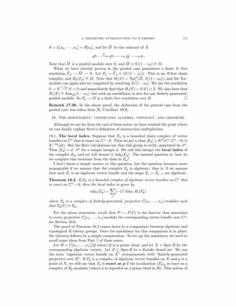
A GEOMETRIC INTRODUCTION TO K-THEORY 117
S = L[x0, · · · , xn] = R[x0], and let M be the cokernel of A:
Sb1A // Sb0 // M // 0 .
Note that M is a graded module over S, and M ⊗ S/(1− x0) ∼= M .What we have already proven in the graded case guarantees a finite S−free
resolution F • → M → 0. Let F• = F • ⊗ (S/(1 − x0)). This is an R-free chaincomplex, and H0(F•) ∼= M . Note that Hi(F ) = TorSi (M , S/(1− x0)), and the Tor-module can again also be computed by resolving S/(1−x0). We use the resolution0→ S
1−x0−→ S → 0 and immediately find that Hi(F ) = 0 if i ≥ 2. We also have thatH1(F ) ∼= Ann eM (1− x0), but such an annihilator is zero for any finitely-generated,graded module. So F• →M is a finite free resolution over R.
Remark 17.26. In the above proof, the deduction of the general case from thegraded case was taken from [E, Corollary 19.8].
18. The denouement: connecting algebra, topology, and geometry
Although we are far from the end of these notes, we have reached the point wherewe can finally explain Serre’s definition of intersection multiplicities.
18.1. The local index. Suppose that E• is a bounded chain complex of vectorbundles on Cn that is exact on Cn−0. Then we get a class [E•] ∈ K0(Cn,Cn−0) ∼=K−2n(pt). But the Bott calculations say that this group is cyclic, generated by βn.Thus [E•] = d · βn for a unique integer d. We call this integer the local index ofthe complex E•, and we will denote it ind0(E•). The natural question is: how dowe compute this invariant from the data in E•?
I don’t know a simple answer to this question, but the question becomes moremanageable if we assume that the complex E• is algebraic: that is, if we assumethat each Ei is an algebraic vector bundle and the maps Ei → Ei−1 are algebraic.
Theorem 18.2. If E• is a bounded complex of algebraic vector bundles on Cn thatis exact on Cn − 0, then the local index is given by
ind0(E•) =∑i
(−1)i dimC Hi(P•)
where P• is a complex of finitely-generated, projective C[x1, . . . , xn]-modules suchthat P•(C) ∼= E•.
For the above statement, recall that P 7→ P (C) is the functor that associatesto every projective C[x1, . . . , xn]-module the corresponding vector bundle over Cn;see Section 10.6.
The proof of Theorem 18.2 comes down to a comparison between algebraic andtopological K-theory groups. Once the machinery for this comparison is in place,the theorem follows by a simple computation. To set up this machinery we need torecall some ideas from Part 1 of these notes.
Let R = C[x1, . . . , xn]/Q where Q is a prime ideal, and let X = SpecR be thecorresponding algebraic variety. Let Z ⊆ SpecR be a Zariski closed set. We usethe term “algebraic vector bundle on X” synonymously with “finitely-generatedprojective over R”. If P• is a complex of algebraic vector bundles on X and p is apoint of X, we will say that P• is exact at p if the localization (P•)p is exact as acomplex of Rp-modules (where p is regarded as a prime ideal in R). This notion of
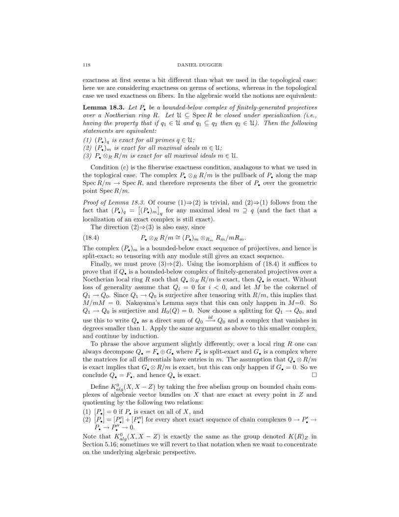
118 DANIEL DUGGER
exactness at first seems a bit different than what we used in the topological case:here we are considering exactness on germs of sections, whereas in the topologicalcase we used exactness on fibers. In the algebraic world the notions are equivalent:
Lemma 18.3. Let P• be a bounded-below complex of finitely-generated projectivesover a Noetherian ring R. Let U ⊆ SpecR be closed under specialization (i.e.,having the property that if q1 ∈ U and q1 ⊆ q2 then q2 ∈ U). Then the followingstatements are equivalent:(1) (P•)q is exact for all primes q ∈ U;(2) (P•)m is exact for all maximal ideals m ∈ U;(3) P• ⊗R R/m is exact for all maximal ideals m ∈ U.
Condition (c) is the fiberwise exactness condition, analagous to what we used inthe toplogical case. The complex P• ⊗R R/m is the pullback of P• along the mapSpecR/m → SpecR, and therefore represents the fiber of P• over the geometricpoint SpecR/m.
Proof of Lemma 18.3. Of course (1)⇒(2) is trivial, and (2)⇒(1) follows from thefact that (P•)q =
[(P•)m
]q
for any maximal ideal m ⊇ q (and the fact that alocalization of an exact complex is still exact).
The direction (2)⇒(3) is also easy, since
P• ⊗R R/m ∼= (P•)m ⊗Rm Rm/mRm.(18.4)
The complex (P•)m is a bounded-below exact sequence of projectives, and hence issplit-exact; so tensoring with any module still gives an exact sequence.
Finally, we must prove (3)⇒(2). Using the isomorphism of (18.4) it suffices toprove that if Q• is a bounded-below complex of finitely-generated projectives over aNoetherian local ring R such that Q• ⊗R R/m is exact, then Q• is exact. Withoutloss of generality assume that Qi = 0 for i < 0, and let M be the cokernel ofQ1 → Q0. Since Q1 → Q0 is surjective after tensoring with R/m, this implies thatM/mM = 0. Nakayama’s Lemma says that this can only happen in M=0. SoQ1 → Q0 is surjective and H0(Q) = 0. Now choose a splitting for Q1 → Q0, anduse this to write Q• as a direct sum of Q0
id−→ Q0 and a complex that vanishes indegrees smaller than 1. Apply the same argument as above to this smaller complex,and continue by induction.
To phrase the above argument slightly differently, over a local ring R one canalways decompose Q• = F•⊕G• where F• is split-exact and G• is a complex wherethe matrices for all differentials have entries in m. The assumption that Q•⊗R/mis exact implies that G•⊗R/m is exact, but this can only happen if G• = 0. So weconclude Q• = F•, and hence Q• is exact.
Define K0alg(X,X −Z) by taking the free abelian group on bounded chain com-
plexes of algebraic vector bundles on X that are exact at every point in Z andquotienting by the following two relations:(1) [P•] = 0 if P• is exact on all of X, and(2) [P•] = [P ′•] + [P ′′• ] for every short exact sequence of chain complexes 0→ P ′• →
P• → P ′′• → 0.Note that K0
alg(X,X − Z) is exactly the same as the group denoted K(R)Z inSection 5.16; sometimes we will revert to that notation when we want to concentrateon the underlying algebraic perspective.
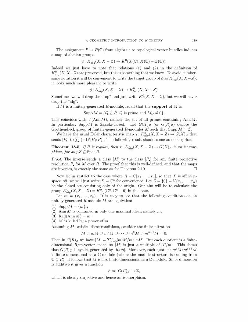
A GEOMETRIC INTRODUCTION TO K-THEORY 119
The assignment P 7→ P (C) from algebraic to topological vector bundles inducesa map of abelian groups
φ : K0alg(X,X − Z)→ K0(X(C), X(C)− Z(C)).
Indeed we just have to note that relations (1) and (2) in the definition ofK0alg(X,X−Z) are preserved, but this is something that we know. To avoid cumber-
some notation it will be convenient to write the target group of φ as K0top(X,X−Z);
it looks much more pleasant to write
φ : K0alg(X,X − Z)→ K0
top(X,X − Z).
Sometimes we will drop the “top” and just write K0(X,X −Z), but we will neverdrop the “alg”.
If M is a finitely-generated R-module, recall that the support of M is
SuppM = Q ⊆ R |Q is prime and MQ 6= 0.This coincides with V (AnnM), namely the set of all primes containing AnnM .In particular, SuppM is Zariski-closed. Let G(X)Z (or G(R)Z) denote theGrothendieck group of finitely-generated R-modules M such that SuppM ⊆ Z.
We have the usual Euler characteristic map χ : K0alg(X,X − Z) → G(X)Z that
sends [P•] to∑i(−1)i[Hi(P )]. The following result should come as no surprise:
Theorem 18.5. If R is regular, then χ : K0alg(X,X − Z)→ G(X)Z is an isomor-
phism, for any Z ⊆ SpecR.
Proof. The inverse sends a class [M ] to the class [P•] for any finite projectiveresolution P• for M over R. The proof that this is well-defined, and that the mapsare inverses, is exactly the same as for Theorem 2.10.
Now let us restrict to the case where R = C[x1, . . . , xn], so that X is affine n-space AnC; we will just write X = Cn for convenience. Let Z = 0 = V (x1, . . . , xn)be the closed set consisting only of the origin. Our aim will be to calculate thegroup K0
alg(X,X − Z) = K0alg(Cn,Cn − 0) in this case.
Let m = (x1, . . . , xn). It is easy to see that the following conditions on anfinitely-generated R-module M are equivalent:(1) SuppM = m ;(2) AnnM is contained in only one maximal ideal, namely m;(3) Rad(AnnM) = m;(4) M is killed by a power of m.Assuming M satisfies these conditions, consider the finite filtration
M ⊇ mM ⊇ m2M ⊇ · · · ⊇ mkM ⊇ mk+1M = 0.
Then in G(R)Z we have [M ] =∑ki=0[m
iM/mi+1M ]. But each quotient is a finite-dimensional R/m-vector space, so [M ] is just a multiple of [R/m]. This showsthat G(R)Z is cyclic, generated by [R/m]. Moreover, each quotient miM/mi+1Mis finite-dimensional as a C-module (where the module structure is coming fromC ⊆ R). It follows thatM is also finite-dimensional as a C-module. Since dimensionis additive it gives a function
dim: G(R)Z → Z,which is clearly surjective and hence an isomorphism.
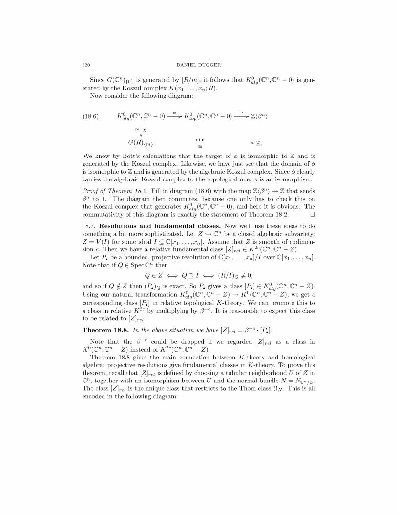
120 DANIEL DUGGER
Since G(Cn)0 is generated by [R/m], it follows that K0alg(Cn,Cn − 0) is gen-
erated by the Koszul complex K(x1, . . . , xn;R).Now consider the following diagram:
K0alg(Cn,Cn − 0)
φ //
χ∼=
K0top(Cn,Cn − 0)
∼= // Z〈βn〉
G(R)mdim∼=
// Z.
(18.6)
We know by Bott’s calculations that the target of φ is isomorphic to Z and isgenerated by the Koszul complex. Likewise, we have just see that the domain of φis isomorphic to Z and is generated by the algebraic Koszul complex. Since φ clearlycarries the algebraic Koszul complex to the topological one, φ is an isomorphism.
Proof of Theorem 18.2. Fill in diagram (18.6) with the map Z〈βn〉 → Z that sendsβn to 1. The diagram then commutes, because one only has to check this onthe Koszul complex that generates K0
alg(Cn,Cn − 0); and here it is obvious. Thecommutativity of this diagram is exactly the statement of Theorem 18.2.
18.7. Resolutions and fundamental classes. Now we’ll use these ideas to dosomething a bit more sophisticated. Let Z → Cn be a closed algebraic subvariety:Z = V (I) for some ideal I ⊆ C[x1, . . . , xn]. Assume that Z is smooth of codimen-sion c. Then we have a relative fundamental class [Z]rel ∈ K2c(Cn,Cn − Z).
Let P• be a bounded, projective resolution of C[x1, . . . , xn]/I over C[x1, . . . , xn].Note that if Q ∈ Spec Cn then
Q ∈ Z ⇐⇒ Q ⊇ I ⇐⇒ (R/I)Q 6= 0,
and so if Q /∈ Z then (P•)Q is exact. So P• gives a class [P•] ∈ K0alg(Cn,Cn − Z).
Using our natural transformation K0alg(Cn,Cn − Z) → K0(Cn,Cn − Z), we get a
corresponding class [P•] in relative topological K-theory. We can promote this toa class in relative K2c by multiplying by β−c. It is reasonable to expect this classto be related to [Z]rel:
Theorem 18.8. In the above situation we have [Z]rel = β−c · [P•].
Note that the β−c could be dropped if we regarded [Z]rel as a class inK0(Cn,Cn − Z) instead of K2c(Cn,Cn − Z).
Theorem 18.8 gives the main connection between K-theory and homologicalalgebra: projective resolutions give fundamental classes in K-theory. To prove thistheorem, recall that [Z]rel is defined by choosing a tubular neighborhood U of Z inCn, together with an isomorphism between U and the normal bundle N = NCn/Z .The class [Z]rel is the unique class that restricts to the Thom class UN . This is allencoded in the following diagram:
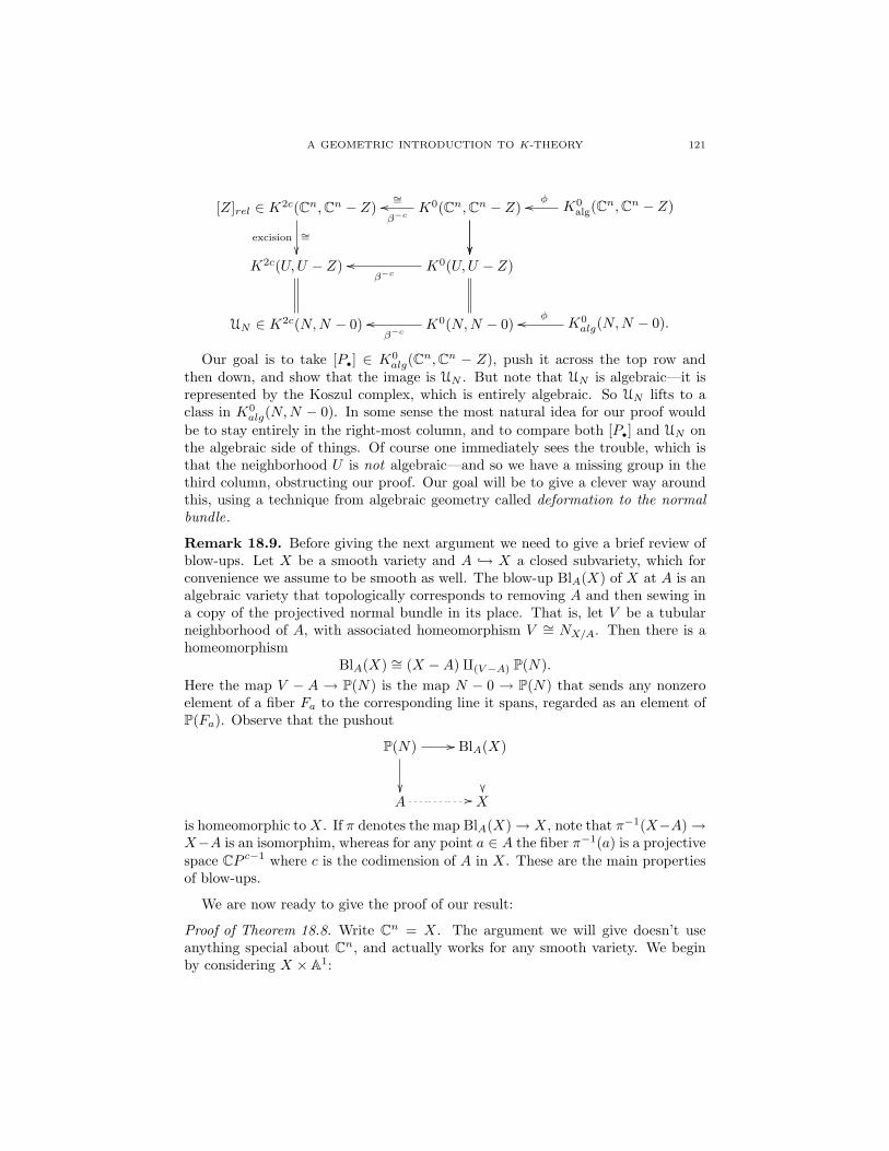
A GEOMETRIC INTRODUCTION TO K-THEORY 121
[Z]rel ∈ K2c(Cn,Cn − Z)
∼=excision
K0(Cn,Cn − Z)β−c
∼=oo
K0alg(Cn,Cn − Z)
φoo
K2c(U,U − Z) K0(U,U − Z)β−c
oo
UN ∈ K2c(N,N − 0) K0(N,N − 0)β−c
oo K0alg(N,N − 0).
φoo
Our goal is to take [P•] ∈ K0alg(Cn,Cn − Z), push it across the top row and
then down, and show that the image is UN . But note that UN is algebraic—it isrepresented by the Koszul complex, which is entirely algebraic. So UN lifts to aclass in K0
alg(N,N − 0). In some sense the most natural idea for our proof wouldbe to stay entirely in the right-most column, and to compare both [P•] and UN onthe algebraic side of things. Of course one immediately sees the trouble, which isthat the neighborhood U is not algebraic—and so we have a missing group in thethird column, obstructing our proof. Our goal will be to give a clever way aroundthis, using a technique from algebraic geometry called deformation to the normalbundle.
Remark 18.9. Before giving the next argument we need to give a brief review ofblow-ups. Let X be a smooth variety and A → X a closed subvariety, which forconvenience we assume to be smooth as well. The blow-up BlA(X) of X at A is analgebraic variety that topologically corresponds to removing A and then sewing ina copy of the projectived normal bundle in its place. That is, let V be a tubularneighborhood of A, with associated homeomorphism V ∼= NX/A. Then there is ahomeomorphism
BlA(X) ∼= (X −A)q(V−A) P(N).Here the map V − A → P(N) is the map N − 0 → P(N) that sends any nonzeroelement of a fiber Fa to the corresponding line it spans, regarded as an element ofP(Fa). Observe that the pushout
P(N) //
BlA(X)
A // X
is homeomorphic toX. If π denotes the map BlA(X)→ X, note that π−1(X−A)→X−A is an isomorphim, whereas for any point a ∈ A the fiber π−1(a) is a projectivespace CP c−1 where c is the codimension of A in X. These are the main propertiesof blow-ups.
We are now ready to give the proof of our result:
Proof of Theorem 18.8. Write Cn = X. The argument we will give doesn’t useanything special about Cn, and actually works for any smooth variety. We beginby considering X × A1:
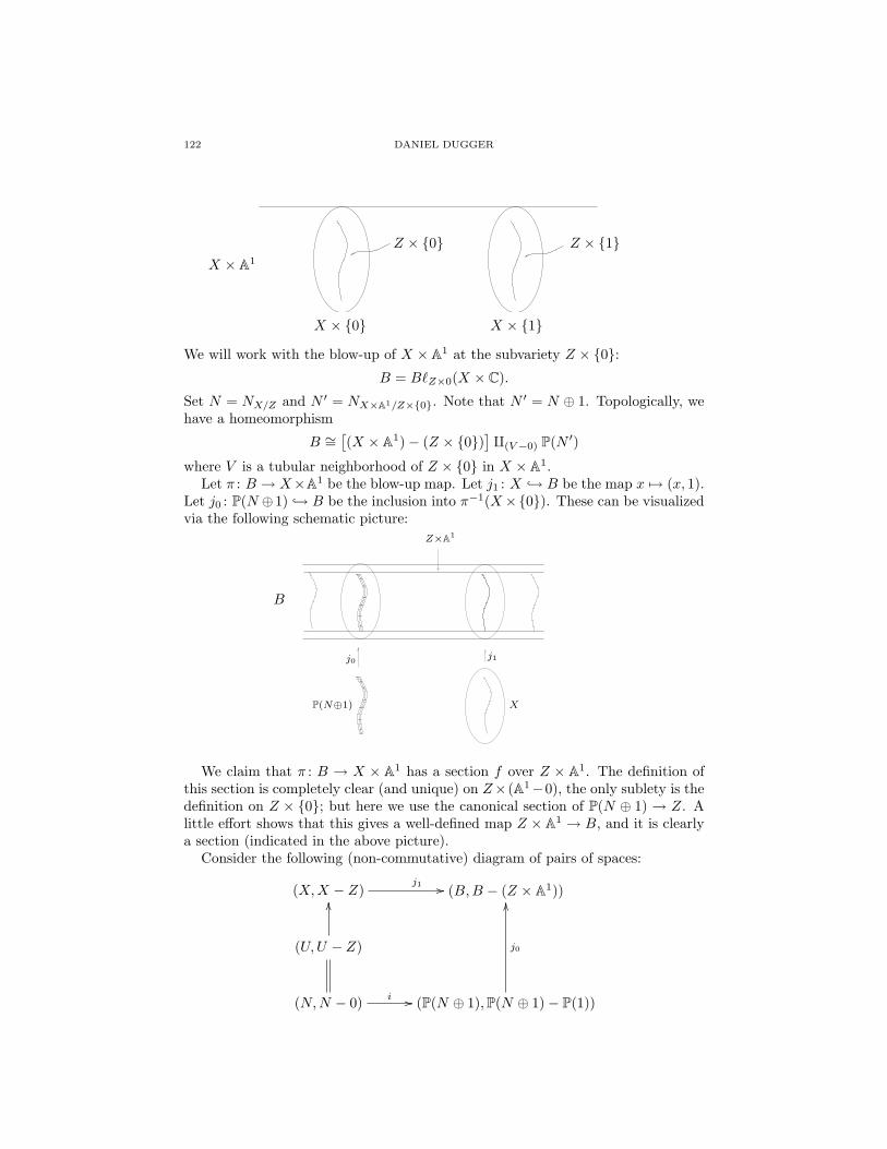
122 DANIEL DUGGER
X × 0 X × 1
X × A1
Z × 0 Z × 1
We will work with the blow-up of X × A1 at the subvariety Z × 0:B = B`Z×0(X × C).
Set N = NX/Z and N ′ = NX×A1/Z×0. Note that N ′ = N ⊕ 1. Topologically, wehave a homeomorphism
B ∼=[(X × A1)− (Z × 0)
]q(V−0) P(N ′)
where V is a tubular neighborhood of Z × 0 in X × A1.Let π : B → X×A1 be the blow-up map. Let j1 : X → B be the map x 7→ (x, 1).
Let j0 : P(N ⊕1) → B be the inclusion into π−1(X×0). These can be visualizedvia the following schematic picture:
Z×A1
B
j0 j1
XP(N⊕1)
We claim that π : B → X × A1 has a section f over Z × A1. The definition ofthis section is completely clear (and unique) on Z× (A1−0), the only sublety is thedefinition on Z × 0; but here we use the canonical section of P(N ⊕ 1) → Z. Alittle effort shows that this gives a well-defined map Z × A1 → B, and it is clearlya section (indicated in the above picture).
Consider the following (non-commutative) diagram of pairs of spaces:
(X,X − Z)j1 // (B,B − (Z × A1))
(U,U − Z)
OO
(N,N − 0) i // (P(N ⊕ 1),P(N ⊕ 1)− P(1))
j0
OO

A GEOMETRIC INTRODUCTION TO K-THEORY 123
Here j1 is the inclusion of the fiber of B → A1 over 1. A little thought shows thatthis diagram commutes up to homotopy. Note that all of the maps are algebraicexcept for the inclusion h : N → X (we implicitly identify N with U here). ApplyK0(−) to obtain the commutative diagram
K0(X,X − Z)
h∗
K0(B,B − (Z × A1))j∗1oo
j∗0
K0(N,N − 0) K0(P(N ⊕ 1),P(N ⊕ 1)− P(1)).i∗oo
(18.10)
The left vertical arrow is dotted only as a reminder that it is not algebraic. Thereis a similar diagram, without the dotted arrow, in which every K0(−) has beenreplaced with K0
alg; and this new diagram maps to the one above.Let Q• be a resolution of OZ×A1 by locally free OB-modules. Then we have the
corresponding class [Q•] ∈ K0(B,B − (Z × A1)). We will show that(1) j∗1 (Q•) is a resolution of OZ on X, and(2) (j0 i)∗(Q•) is a resolution of the structure sheaf of the zero-section on N .From (1) it follows that there is a chain homotopy equivalence j∗1 (Q•) ' P•, whereP• is our chosen resolution of OZ on X. Hence j∗1 ([Q•]) = [P•] in K0
alg(X,X − Z).From (2) it follows that there is a chain homotopy equivalence (j0i)∗(Q•) ' J∗p∗N,∆,since both gives resolutions of the structure sheaf of the zero section on N . Hencei∗(j∗0 ([Q•])) = UN in K0
alg(N,N − 0). Now push all of this into topological K0
and use the commutativity of (18.10) to obtain that h∗([P•]) = UN . But h∗ is anisomorphism, and [Z]rel was defined to be the unique class in K0(X,X − Z) thatmaps to UN via h∗. So [P•] = [Z]rel.
So the proof reduces to checking the algebraic facts (1) and (2). To do so, startwith the following diagram
B1// j1 //
B
X × 1 // //
X × A1
1 // A1
(18.11)
where B1 is the fiber of B → A1 over 1 (note that B1∼= X). Every square in this
diagram is a pullback, including the outer square (which is more of a rectangle).Applying j∗1 to Q• amounts to pulling back along 1 → A1 (or algebraically,tensoring over C[t] with C[t]/(t − 1)). But note that B → A1 is flat—a map froma variety to a curve is flat as long as it is dominant, which this clearly is. So OBis flat over A1, and it is trivial that the OB-module OZ×A1 is flat over A1. So thecomplex Q• → OZ×A1 → 0 is an exact sequence of sheaves that are flat over A1,therefore the pullback to B1 is still exact. This proves (1).
The proof of (2) is very similar. Consider the analog of diagram (18.11) builtaround the inclusions B0 → B and 0 → A1. We argue as above that the pullbackof Q• → OZ×A1 to B0 is still exact. Note that B0 = BlZ(X) qP(N) P(N ⊕ 1), withBlZ(X) a closed subscheme. So B0 − BlZ(X) = P(N ⊕ 1) − P(N) = N . The
124 DANIEL DUGGER
bundle N is therefore an open subscheme of B0, and of course the inclusion of anopen subscheme is flat—so restricting further to N still preserves exactness. Thelast thing to check is that restricting OZ×A1 to B0 gives the structure sheaf for thecanonical section of P(N ⊕ 1) (which then corresponds to the zero section of Nunder N → P(N ⊕ 1))—but this is obvious.
Remark 18.12. The technique used in the above proof, centering around thevariety B, is called “deformation to the normal bundle”. It was used extensivelyin papers by Fulton and Macpherson in the 1970s, and has a prominent role in thebook [F]. The technique gives a substitute in algebraic geometry for the role playedby tubular neighborhoods in topology.
As a consequence of Theorem 18.8 we can now obtain Serre’s formula for inter-section multiplicities:
Corollary 18.13. Let Z and W be smooth, closed subvarieties of Cn such thatZ ∩ W = 0. Then i(Z,W ; 0) =
∑(−1)i dim Tori(R/I,R/J), where R =
C[x1, . . . , xn] and I and J are the ideals of functions vanishing on Z and W , re-spectively.
Proof. Start with the relative fundamental classes [Z]rel ∈ K2c(Cn,Cn − Z) and[W ]rel ∈ K2d(Cn,Cn−W ), where c and d are the codimensions of Z and W insideof Cn. Note that since 0 is an isolated point of intersection we must have c+ d ≥ n(this is an algebraic lemma, see ????). There are in some sense two cases, dependingon whether c+d = n or c+d > n. In the former case, multiplying our fundamentalclasses together we get
[Z]rel · [W ]rel ∈ K2n(Cn,Cn − (Z ∩W )) = K2n(Cn,Cn − 0).
Note thatK2n(Cn,Cn−0) ∼= Z and is generated by [0]rel. The topological definitionof i(Z,W ; 0) is that it is the unique integer for which
[Z]rel · [W ]rel = i(Z,W ; 0) · [0]rel(18.14)
This definition works in any complex-oriented cohomology theory.If c+d > n then it is clear that Z and W may be moved near 0 (in the topological
setting) so that they do not intersect at all, and therefore [Z]rel · [W ]rel = 0.Equation (18.14) is still a valid definition, it just yields that i(Z,W ; 0) = 0 here.
The key to the proof is simply realizing that all of our constructions can be liftedback into K0
alg. Let P• → R/I and Q• → R/J be bounded free resolutions. Then[Z]rel = β−c · [P•] and [W ]rel = β−d · [Q•]. So [Z]rel · [W ]rel = β−c−d · [P.⊗R Q] ∈K2(c+d)(Cn,Cn − 0). Recall that K0(Cn,Cn − 0) ∼= Z and is generated by theKoszul complex J∗. Recall as well that [0]rel = β−n · [J∗], by definition. If we write[P ⊗R Q] = s[J∗] for s ∈ Z, then we have the formula
s · β−c−d · [J∗] = i(Z,W ; 0) · β−n · [J∗].If c+d = n then the formula implies s = i(Z,W ; 0). If c+d 6= n then the only waythe formula can be true is if both sides are zero, in which case s = 0 = i(Z,W ; 0).So s = i(Z,W ; 0) in either case.
To conclude the proof we just note that the Local Index Theorem (18.2) givess =
∑i(−1)i dimC Hi(P ⊗R Q), and Hi(P ⊗Q) ∼= Tori(R/I,R/J).
Exercise 18.15. Suppose that Z and W are smooth algebraic subvarieties of Cnsuch that Z ∩W = p1, . . . , pd.

A GEOMETRIC INTRODUCTION TO K-THEORY 125
(a) Choose a polynomial f ∈ C[x1, . . . , xn] such that f(pi) = 0 for i > 1 andf(p1) 6= 0, and let S = Rf . Let U = SpecRf ⊆ Cn be the corresponding Zariskiopen set. Convince yourself that it is reasonable to define the intersectionmultiplicity i(Z,W ; p1) by the formula
[Z]rel,U · [W ]rel,U = i(Z,W ; p1) · β−n · [p1]rel,Uwhere [Z]rel,U is the image of [Z]rel under K∗(Cn,Cn − Z) → K∗(U,U − Z),and similarly for [W ]rel,U and [p1]rel,U . In particular, convince yourself thatthis is independent of the choice of f .
(b) Next, modify the proof of Corollary 18.13 to show that
i(Z,W ; p1) =∑
(−1)i dimC Tori(R/I,R/J)f
where I and J are the ideals corresponding to Z and W .(c) If M is a finitely-generated module over Rf such that SuppM = p (p a
maximal ideal of R), prove that M = Mp. Deduce that
i(Z,W ; p1) =∑
(−1)i dimC Tori(R/I,R/J)p1 .
Corollary 18.13 (and Exercise 18.15) in some sense brings to a close the mainquestions we raised at the beginning of these notes. We have now seen why Serre’salternating sum of Tor’s definition of intersection multiplicity is the ‘correct’ one,and how this ties in to the study of K-theory.
19. More about relative K-theory
Our aim in this section is to revisit the issue of relative K-theory and give theproof of Theorem 17.16. The ideas behind the proof are interesting and have theirown intrinsic appeal, but in fact they hardly ever resurface outside the confinesof this one argument. This section should be regarded as giving some technicalinformation which is not necessary for anything later in the notes.
Throughout this section (X,A) will be a finite CW -pair, unless otherwise noted.Recall the group K(X,A) introduced in Definition 17.6, made from bounded com-plexes of vector bundles on X that are exact on A. We take several steps aimed atanalyzing these groups:(1) Instead of studying K(X,A) directly we look instead at a certain set of equiv-
alence classes of complexes. This set is a monoid whose group completion isK(X,A), but it has the property that the equivalence classes are a bit easierto get our hands on.
(2) Rather than consider all bounded complexes, we consider complexes which areconcentrated in degrees between 0 and n, for some fixed n ≥ 1. We provethat all choices of n give rise to the same theory; so in some sense the use ofchain complexes is overkill, as it suffices to just look at complexes of length 1.(The use of all chain complexes makes for a more natural theory, however—forexample, the tensor product of two complexes of length 1 is a complex of length2, and can only be turned back into a complex of length 1 by a cumbersomeprocess).
(3) Finally, and most importantly, we replace our consideration of chain complexesby that of a related but different construct. Namely, we consider Z-gradedcollections of vector bundles Ei together with an exact differential definedonly over the set A (that is, a differential on (E•)|A). Let us call such things

126 DANIEL DUGGER
“A-relative chain complexes”. It turns out that every A-relative chain complexmay be extended to give an ordinary chain complex (that is exact on A), andthe space of all possible extensions is contractible. So homotopically speakingthere is no real difference between the theories obtained from the two notions.The A-relative chain complexes turn out to give a theory that is a bit easier tomanipulate, essentially because one doesn’t have to deal with extraneous data.
19.1. Relative chain complexes. Let Ch(X,A) denote the category whose ob-jects are bounded chain complexes of vector bundles on X that are exact on A.A map in this category is simply a map of chain complexes of vector bundles. Incontrast to this, let Ch(X,A)A denote the category whose objects are collectionsEi of vector bundles on X, all but finitely-many of which are zero, together withmaps d : Ei+1|A→ Ei|A making the restriction E•|A into an exact chain complex ofvector bundles on A. A map E → E′ in Ch(X,A)A is a collection of maps Ei → E′iof vector bundles on X that commute with the maps d where defined (i.e., over theset A). An object in Ch(X,A)A will be called an A-relative chain complex.
Note the difference between Ch(X,A) and Ch(X,A)A: in the former the differ-entials are defined on all of X, whereas in the latter they are only defined on A.Observe that there is an evident functor Ch(X,A) → Ch(X,A)A, which we willdenote E 7→ E(A).
Say that two complexes E• and E′• in Ch(X,A) are homotopic if there is anobject E in Ch(X× I,A× I) together with isomorphisms E|X×0
∼= E• and E|X×1∼=
E′• in Ch(X,A). Write this relation as E• ∼h F•. Likewise, define two complexes E•
and E′• in Ch(X,A)A to be homotopic if there is an object E in Ch(X×I,A×I)A×Itogether with isomorphisms E|X×0
∼= E• and E|X×1∼= E′• in Ch(X,A)A. In each
of these two settings the notion of homotopy is readily seen to be an equivalencerelation.
We will also need a second equivalence relation on chain complexes. Say that twocomplexes E• and E′• in Ch(X,A) are stably equivalent if there exist elementarycomplexes (see Definition 17.9) P1, . . . , Pr, Q1, . . . , Qs in Ch(X,A) such that
E ⊕ P1 ⊕ · · · ⊕ Pr ∼= E′ ⊕Q1 ⊕ · · · ⊕Qs.Write this as E• ∼st E′•. We define a similar equivalence relation on the objects ofCh(X,A)A.
Let Chn(X,A) be the full subcategory of Ch(X,A) consisting of chain complexesE• such that Ei = 0 when i /∈ [0, n], and let Chn(X,A)A be the analogous sub-category of A-relative complexes. It will be convenient to allow the index n to be∞ here. Let Ln(X,A) and Ln(X,A)A denote the sets of isomorphism classes ofobjects in these two categories.
Write Ln(X,A)h for the equivalence classes of Ln(X,A) under the homotopyrelation. Also, write Ln(X,A)st for the equivalence classes of Ln(X,A) underthe stable-equivalence relation. Finally, write Ln(X,A)h,st for the equivalenceclasses generated by combination of these two types of equivalence. Note that wealso have sets Ln(X,A)hA, Ln(X,A)stA , and Ln(X,A)h,stA . The restriction functorChn(X,A)→ Chn(X,A)A clearly induces maps of sets Ln(X,A)h,st → Ln(X,A)h,stA
and so forth.Note that direct sum of complexes makes Ln(X,A) into a monoid, and similarly
for Ln(X,A)h, Ln(X,A)st, and Ln(X,A)h,st. The same remark holds for the A-relative versions.

A GEOMETRIC INTRODUCTION TO K-THEORY 127
19.2. Comparing complexes to A-relative complexes. Our first importantresult is the following:
Proposition 19.3. For any n ≥ 1 the map Ln(X,A)h,st → Ln(X,A)h,stA is abijection.
We start with a lemma:
Lemma 19.4. The functor Ch(X,A)→ Ch(X,A)A is surjective on objects. Addi-tionally, if E1 and E2 are objects in Ch(X,A)A such that E1(A) ∼= E2(A) then E1
and E2 are homotopic.
Proof. Given a collection of complex vector spaces Vi, i ∈ Z, let Ch-struct(V ) ⊆∏i Hom(Vi+1, Vi) denote the collection of sequences (di)i∈Z satisfying di di+1 = 0
for all i. Regard Ch-struct(V ) as a topological space by giving it the subspacetopology. Note that if d ∈ Ch-struct(V ) then t · d ∈ Ch-struct(V ) for any t ∈ C,and letting t 7→ 0 thereby gives a contracting homotopy showing that Ch-struct(V )is contractible.
Now suppose that Eii∈Z is a collection of vector bundles on X having theproperty that only finitely many are nonzero. Let Ch-struct(E)→ X be the evidentmap whose fiber over a point x is Ch-struct((Ei)x). The assumption that thereare only finitely many Ei implies that each x has a neighborhood over which allthe bundles are trivial, and from this it readily follows that Ch-struct(E)→ X is afiber bundle. As the fibers are contractible, it is also a weak homotopy equivalence.
Note that making Ei into a chain complex is precisely the same as givinga section of Ch-struct(E) → X. Likewise, equipping Ei with a chain complexdifferential over A is the same as giving a section defined over A.
Suppose given an object E in Ch(X,A)A. Consider the diagram
A //
Ch-struct(E)
'
X // X
(19.5)
where the top horizontal map encodes the differentials on E. Since A → X isa cofibration and Ch-struct(E) → X is a trivial fibration, there is a lifting X →Ch-struct(E). This lifting precisely gives a chain complex structure on Ei, definedon all of X, that extends the one defined over A. This proves that the functorE 7→ E(A) is surjective on objects.
Next observe that if f : Y → X is any map then Ch-struct(f∗E) is canonicallyidentified with the pullback of Y → X ← Ch-struct(E). This is an easy exercise.Suppose that (E, s) and (E, s′) are two preimages in Ch(X,A) for the same objectE in Ch(X,A)A. Then s and s′ correspond to two liftings in the square (19.5).Given this data, form the new diagram
(X × 0)q(A×I) (X × 1) //
Ch-struct(E)
'
X × I π // X
where π : X × I → X is the projection, A × I → Ch-struct(E) is the constanthomotopy, and the top horizontal map equals s and s′ on the two copies of X.

128 DANIEL DUGGER
Once again, the diagram has a lifting. The resulting map X × I → Ch-struct(E)corresponds to a section of Ch-struct(π∗E)→ X × I, and so specifies a complex ofvector bundles on X× I. It is clear that the differentials are constant (with respectto ‘time’) on A × I, so the complex lives in Ch(X × I, A × I). By construction itrestricts to the two liftings (E, s) and (E, s′) at times 0 and 1.
Now suppose that E and F are objects in Ch(X,A) and that E(A) ∼= F (A). Sothere are isomorphisms fi : Ei → Fi of bundles over X which, when restricted toA, commute with the differentials d. Let d′i be the composite
Eifi−→ Fi
d−→ Fi−1
f−1i−1−→ Ei−1.
Note that the d′ maps give a chain complex structure on Ei; call this new chaincomplex E′. We have E′ ∼= F as objects in Ch(X,A). Observe that d′|A = d|A,and so E(A) = E′(A). It follows by what we have already proven that E and E′
are homotopic in Ch(X,A). Since E′ and F are (trivially) homotopic, transitivitygives that E is homotopic to F .
Remark 19.6. The above proof was written in part to demonstrate the techniqueof translating a desired task into a lifting problem. This is a useful technique thatwe will need again later in this section. However, it is worth pointing out that inthe particular cases from the above proof the lifting problems could be solved ina very concrete and simple way. If (Y,B) is a CW -pair and E• is an object inCh(Y,B)B , we extend the differentials from B to all of Y by an induction over thecells of Y − B. If en is such a cell, we assume inductively that the differentialshave been defined over the boundary. Identifying the cell with the disk Dn, pointsin the interior of the cell have the form tx for x ∈ ∂Dn and t ∈ [0, 1). Definethe differential over tx to be t times the differential over x. This clearly gives therequired extension.
Proof of Proposition 19.3. It remains to prove that Ln(X,A)h,st → Ln(X,A)h,stA isinjective. Let E and F be two objects in Chn(X,A). It will suffice to prove that(1) if E(A) ∼h F (A) then E = F in Ln(X,A)h,st, and(2) if E(A) ∼st F (A) then E = F in Ln(X,A)h,st.
For suppose that E(A) and F (A) are identified in Ln(X,A)h,stA . Then there is afinite chain of objects E1, E2, . . . , Er in Chn(X,A)A such that E1 = E(A), Er =F (A), and for each i either Ei ∼h Ei+1 or Ei ∼st Ei+1. By Lemma 19.4 there arechain complexes Ei ∈ Chn(X,A) such that Ei(A) = Ei, for each i. We can chooseE1 = E and Er = F , and we do so. By iterated applications of (1) and (2) we thenknow that E1, E2, . . . , Er are all identified in Ln(X,A)h,st, and in particular E andF are identified. This is what we needed to prove.
We turn to the proofs of (1) and (2). Suppose that E(A) ∼h F (A). Then thereexists an E ∈ Ch(X × I,A× I)A×I together with isomorphisms E|X×0
∼= E(A) andE|X×1
∼= F (A). By Lemma 19.4 there is an E ∈ Ch(X×I,A×I) such that E(A) = E.So E|X×0 and E|X×1 are homotopic. Moreover, we have E|X×0(A) ∼= E(A), and soby Lemma 19.4 E|X×0 is homotopic to E. The same reasoning gives that E|X×1 ishomotopic to F . By transitivity, E is homotopic to F .
Finally, suppose that E(A) ∼st F (A). So there exist elementary complexesP1, . . . , Pr and Q1, . . . , Qs such that E(A)⊕
⊕i Pi∼= F (A)⊕
⊕j Qj . Let P = ⊕iPi
and Q = ⊕jQj , and observe that these belong to Chn(X,A) (i.e, the differentials
A GEOMETRIC INTRODUCTION TO K-THEORY 129
are defined over all of X). Then (E ⊕ P )(A) ∼= (F ⊕ Q)(A), and so Lemma 19.4tells us that E⊕P and F ⊕Q are homotopic. Consequently, E and F are identifiedin Ln(X,A)h,st.
19.7. Where we are headed. The group K(X,A) is readily checked to be thegroup completion of the monoid L∞(X,A)h,st (use Proposition 17.10). By Propo-sition 19.3 this is the same as the group-completion of L∞(X,A)h,stA , and we willnow focus entirely on this latter object.
Note that L∞(X,A)h,stA is the colimit of the directed system
L1(X,A)h,stA −→ L2(X,A)h,stA −→ L3(X,A)h,stA −→ · · ·
Our next task will be reduce the study of L∞(X,A)h,stA to the much more accessibleobject L1(X,A)h,stA . We will show that the maps Ln(X,A)h,stA → Ln+1(X,A)h,stA
are bijective for all n ≥ 1. This will be based on a strange technique for folding thetop group of an exact complex two degrees lower down, to construct a new complexthat happens to also be exact. We pause to describe the algebra underlying thistechnique.
19.8. An unusual construction from homological algebra. Let V be an exactcomplex of vector spaces and assume that Vi = 0 for i > n. (The complex couldactually consist of projectives over some ring, but let us stick with the simplersetting). Since the complex is exact there exists a contracting homotopy: mapse : Vi → Vi+1 such that de + ed = id. Let ΓV be the following chain complex,concentrated in degrees smaller than n and agreeing with V in degrees smallerthan n− 2:
0 // Vn−1// Vn−2 ⊕ Vn // Vn−3
// Vn−4// · · ·
x // (dx, ex)
(a, b) // da.
It is an elementary exercise to prove that ΓV is exact, but this will also followdirectly from the two decompositions we produce next.
For any vector space W and any k ∈ Z, write Dk(W ) for the chain complexconsisting of W in degrees k and k + 1, where the differential is the identity.
Returning to our chain complex V with contracting homotopy e, note that forx ∈ Vn one has ed(x) = x. Using this, we can write down a natural chain mapV → Dn−1(Vn) that is the identity in degree n and the map e : Vn−1 → Vn in degreen−1. Let ΓV be the desuspension of the mapping cone of this map; specifically, ΓVis the following chain complex, concentrated in dimensions at most n and agreeingwith V in dimensions smaller than n− 2:
0 // Vn // Vn−1 ⊕ Vn // Vn−2 ⊕ Vn // Vn−3// Vn−4
// · · ·
x // (dx,−x) (x, y) // dx
(a, b) // (da, ea+ b)
There is a canonical inclusionDn−2(Vn) → ΓV , and the quotient is V . Moreover,this inclusion has a canonical splitting χ defined by χ(a, b) = ea + b for (a, b) ∈
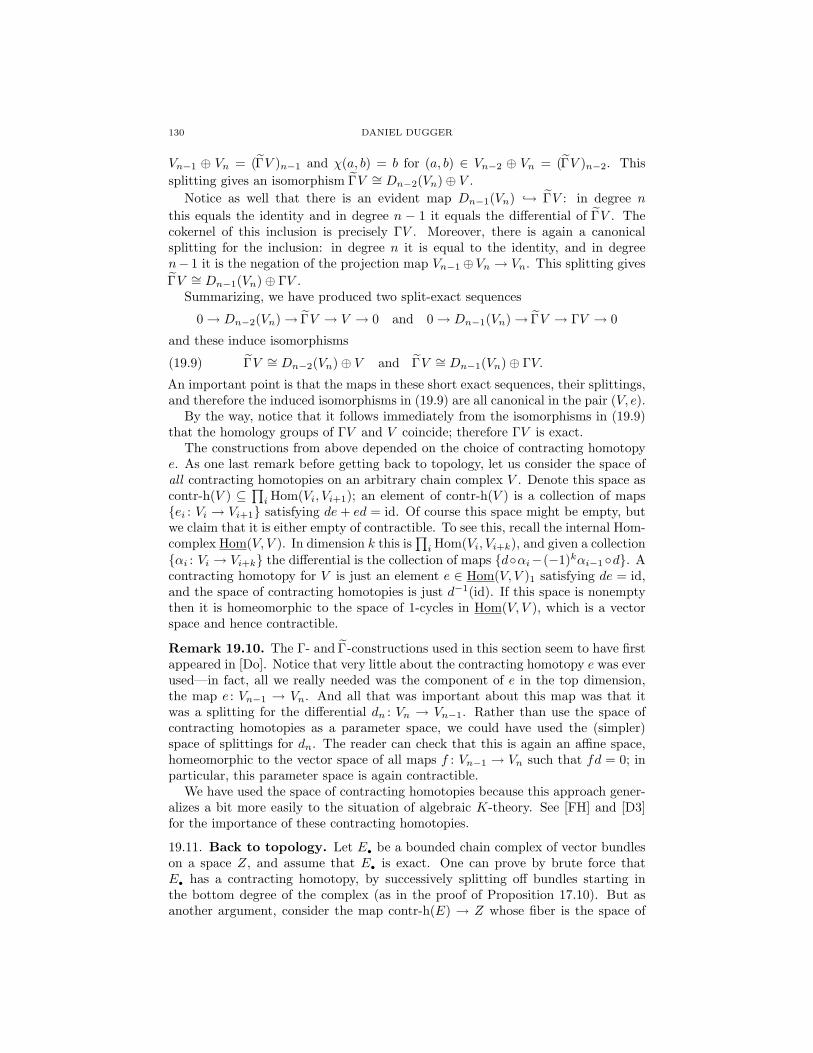
130 DANIEL DUGGER
Vn−1 ⊕ Vn = (ΓV )n−1 and χ(a, b) = b for (a, b) ∈ Vn−2 ⊕ Vn = (ΓV )n−2. Thissplitting gives an isomorphism ΓV ∼= Dn−2(Vn)⊕ V .
Notice as well that there is an evident map Dn−1(Vn) → ΓV : in degree n
this equals the identity and in degree n − 1 it equals the differential of ΓV . Thecokernel of this inclusion is precisely ΓV . Moreover, there is again a canonicalsplitting for the inclusion: in degree n it is equal to the identity, and in degreen− 1 it is the negation of the projection map Vn−1⊕Vn → Vn. This splitting givesΓV ∼= Dn−1(Vn)⊕ ΓV .
Summarizing, we have produced two split-exact sequences
0→ Dn−2(Vn)→ ΓV → V → 0 and 0→ Dn−1(Vn)→ ΓV → ΓV → 0
and these induce isomorphisms
ΓV ∼= Dn−2(Vn)⊕ V and ΓV ∼= Dn−1(Vn)⊕ ΓV.(19.9)
An important point is that the maps in these short exact sequences, their splittings,and therefore the induced isomorphisms in (19.9) are all canonical in the pair (V, e).
By the way, notice that it follows immediately from the isomorphisms in (19.9)that the homology groups of ΓV and V coincide; therefore ΓV is exact.
The constructions from above depended on the choice of contracting homotopye. As one last remark before getting back to topology, let us consider the space ofall contracting homotopies on an arbitrary chain complex V . Denote this space ascontr-h(V ) ⊆
∏i Hom(Vi, Vi+1); an element of contr-h(V ) is a collection of maps
ei : Vi → Vi+1 satisfying de+ ed = id. Of course this space might be empty, butwe claim that it is either empty of contractible. To see this, recall the internal Hom-complex Hom(V, V ). In dimension k this is
∏i Hom(Vi, Vi+k), and given a collection
αi : Vi → Vi+k the differential is the collection of maps dαi−(−1)kαi−1d. Acontracting homotopy for V is just an element e ∈ Hom(V, V )1 satisfying de = id,and the space of contracting homotopies is just d−1(id). If this space is nonemptythen it is homeomorphic to the space of 1-cycles in Hom(V, V ), which is a vectorspace and hence contractible.
Remark 19.10. The Γ- and Γ-constructions used in this section seem to have firstappeared in [Do]. Notice that very little about the contracting homotopy e was everused—in fact, all we really needed was the component of e in the top dimension,the map e : Vn−1 → Vn. And all that was important about this map was that itwas a splitting for the differential dn : Vn → Vn−1. Rather than use the space ofcontracting homotopies as a parameter space, we could have used the (simpler)space of splittings for dn. The reader can check that this is again an affine space,homeomorphic to the vector space of all maps f : Vn−1 → Vn such that fd = 0; inparticular, this parameter space is again contractible.
We have used the space of contracting homotopies because this approach gener-alizes a bit more easily to the situation of algebraic K-theory. See [FH] and [D3]for the importance of these contracting homotopies.
19.11. Back to topology. Let E• be a bounded chain complex of vector bundleson a space Z, and assume that E• is exact. One can prove by brute force thatE• has a contracting homotopy, by successively splitting off bundles starting inthe bottom degree of the complex (as in the proof of Proposition 17.10). But asanother argument, consider the map contr-h(E) → Z whose fiber is the space of
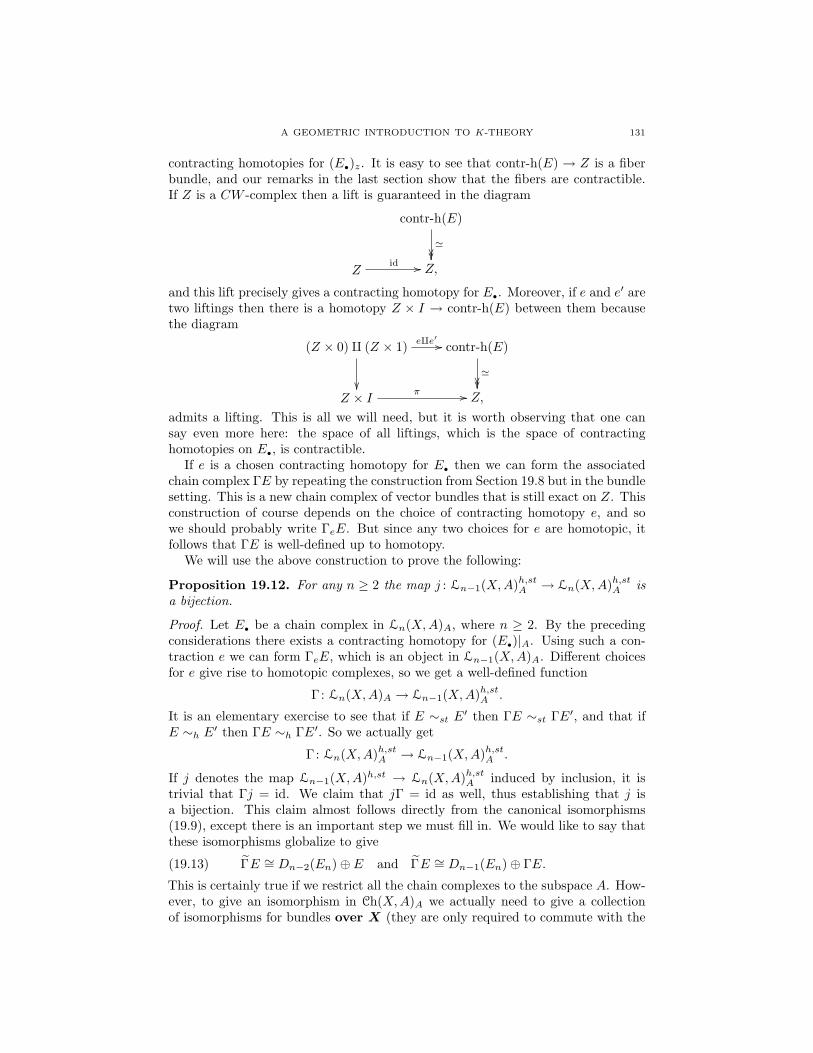
A GEOMETRIC INTRODUCTION TO K-THEORY 131
contracting homotopies for (E•)z. It is easy to see that contr-h(E) → Z is a fiberbundle, and our remarks in the last section show that the fibers are contractible.If Z is a CW -complex then a lift is guaranteed in the diagram
contr-h(E)
'
Zid // Z,
and this lift precisely gives a contracting homotopy for E•. Moreover, if e and e′ aretwo liftings then there is a homotopy Z × I → contr-h(E) between them becausethe diagram
(Z × 0)q (Z × 1) eqe′ //
contr-h(E)
'
Z × I π // Z,
admits a lifting. This is all we will need, but it is worth observing that one cansay even more here: the space of all liftings, which is the space of contractinghomotopies on E•, is contractible.
If e is a chosen contracting homotopy for E• then we can form the associatedchain complex ΓE by repeating the construction from Section 19.8 but in the bundlesetting. This is a new chain complex of vector bundles that is still exact on Z. Thisconstruction of course depends on the choice of contracting homotopy e, and sowe should probably write ΓeE. But since any two choices for e are homotopic, itfollows that ΓE is well-defined up to homotopy.
We will use the above construction to prove the following:
Proposition 19.12. For any n ≥ 2 the map j : Ln−1(X,A)h,stA → Ln(X,A)h,stA isa bijection.
Proof. Let E• be a chain complex in Ln(X,A)A, where n ≥ 2. By the precedingconsiderations there exists a contracting homotopy for (E•)|A. Using such a con-traction e we can form ΓeE, which is an object in Ln−1(X,A)A. Different choicesfor e give rise to homotopic complexes, so we get a well-defined function
Γ: Ln(X,A)A → Ln−1(X,A)h,stA .
It is an elementary exercise to see that if E ∼st E′ then ΓE ∼st ΓE′, and that ifE ∼h E′ then ΓE ∼h ΓE′. So we actually get
Γ: Ln(X,A)h,stA → Ln−1(X,A)h,stA .
If j denotes the map Ln−1(X,A)h,st → Ln(X,A)h,stA induced by inclusion, it istrivial that Γj = id. We claim that jΓ = id as well, thus establishing that j isa bijection. This claim almost follows directly from the canonical isomorphisms(19.9), except there is an important step we must fill in. We would like to say thatthese isomorphisms globalize to give
ΓE ∼= Dn−2(En)⊕ E and ΓE ∼= Dn−1(En)⊕ ΓE.(19.13)
This is certainly true if we restrict all the chain complexes to the subspace A. How-ever, to give an isomorphism in Ch(X,A)A we actually need to give a collectionof isomorphisms for bundles over X (they are only required to commute with the
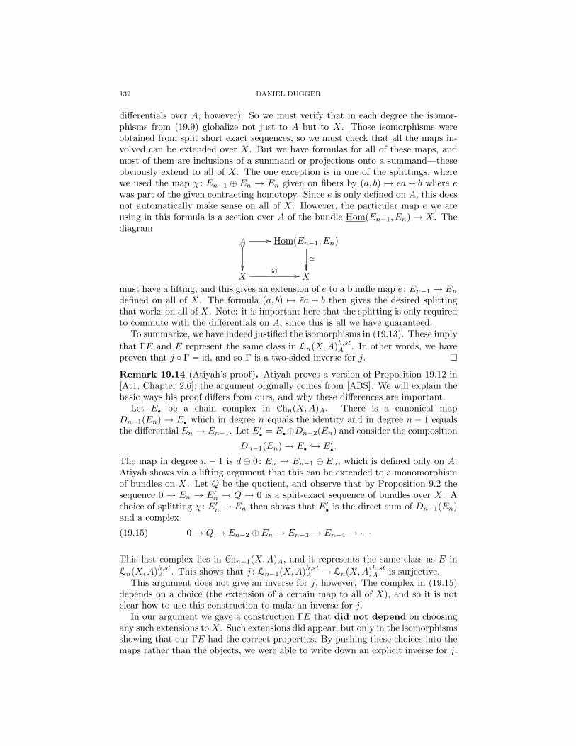
132 DANIEL DUGGER
differentials over A, however). So we must verify that in each degree the isomor-phisms from (19.9) globalize not just to A but to X. Those isomorphisms wereobtained from split short exact sequences, so we must check that all the maps in-volved can be extended over X. But we have formulas for all of these maps, andmost of them are inclusions of a summand or projections onto a summand—theseobviously extend to all of X. The one exception is in one of the splittings, wherewe used the map χ : En−1 ⊕ En → En given on fibers by (a, b) 7→ ea + b where ewas part of the given contracting homotopy. Since e is only defined on A, this doesnot automatically make sense on all of X. However, the particular map e we areusing in this formula is a section over A of the bundle Hom(En−1, En) → X. Thediagram
A //
Hom(En−1, En)
'
Xid // X
must have a lifting, and this gives an extension of e to a bundle map e : En−1 → Endefined on all of X. The formula (a, b) 7→ ea + b then gives the desired splittingthat works on all of X. Note: it is important here that the splitting is only requiredto commute with the differentials on A, since this is all we have guaranteed.
To summarize, we have indeed justified the isomorphisms in (19.13). These implythat ΓE and E represent the same class in Ln(X,A)h,stA . In other words, we haveproven that j Γ = id, and so Γ is a two-sided inverse for j.
Remark 19.14 (Atiyah’s proof). Atiyah proves a version of Proposition 19.12 in[At1, Chapter 2.6]; the argument orginally comes from [ABS]. We will explain thebasic ways his proof differs from ours, and why these differences are important.
Let E• be a chain complex in Chn(X,A)A. There is a canonical mapDn−1(En) → E• which in degree n equals the identity and in degree n − 1 equalsthe differential En → En−1. Let E′• = E•⊕Dn−2(En) and consider the composition
Dn−1(En)→ E• → E′•.
The map in degree n − 1 is d ⊕ 0: En → En−1 ⊕ En, which is defined only on A.Atiyah shows via a lifting argument that this can be extended to a monomorphismof bundles on X. Let Q be the quotient, and observe that by Proposition 9.2 thesequence 0 → En → E′n → Q → 0 is a split-exact sequence of bundles over X. Achoice of splitting χ : E′n → En then shows that E′• is the direct sum of Dn−1(En)and a complex
0→ Q→ En−2 ⊕ En → En−3 → En−4 → · · ·(19.15)
This last complex lies in Chn−1(X,A)A, and it represents the same class as E inLn(X,A)h,stA . This shows that j : Ln−1(X,A)h,stA → Ln(X,A)h,stA is surjective.
This argument does not give an inverse for j, however. The complex in (19.15)depends on a choice (the extension of a certain map to all of X), and so it is notclear how to use this construction to make an inverse for j.
In our argument we gave a construction ΓE that did not depend on choosingany such extensions toX. Such extensions did appear, but only in the isomorphismsshowing that our ΓE had the correct properties. By pushing these choices into themaps rather than the objects, we were able to write down an explicit inverse for j.
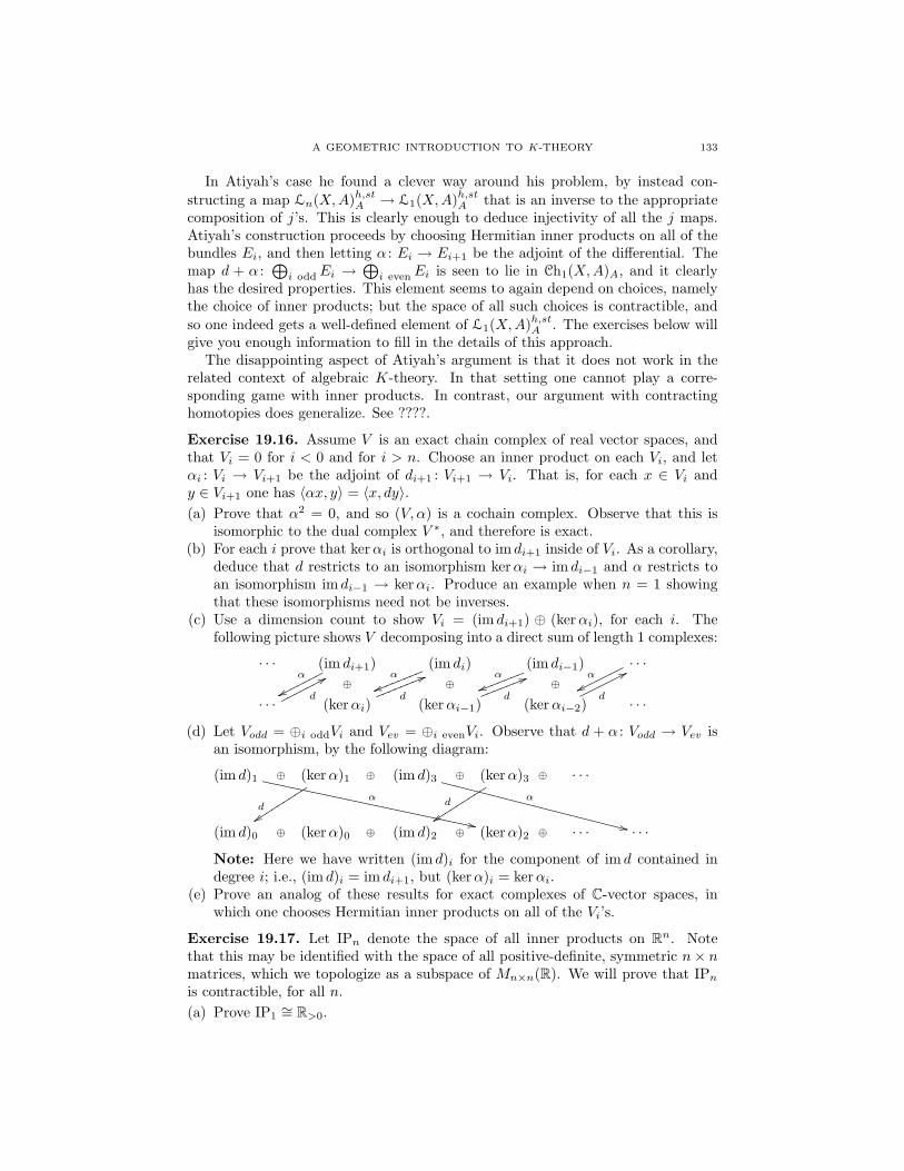
A GEOMETRIC INTRODUCTION TO K-THEORY 133
In Atiyah’s case he found a clever way around his problem, by instead con-structing a map Ln(X,A)h,stA → L1(X,A)h,stA that is an inverse to the appropriatecomposition of j’s. This is clearly enough to deduce injectivity of all the j maps.Atiyah’s construction proceeds by choosing Hermitian inner products on all of thebundles Ei, and then letting α : Ei → Ei+1 be the adjoint of the differential. Themap d + α :
⊕i oddEi →
⊕i evenEi is seen to lie in Ch1(X,A)A, and it clearly
has the desired properties. This element seems to again depend on choices, namelythe choice of inner products; but the space of all such choices is contractible, andso one indeed gets a well-defined element of L1(X,A)h,stA . The exercises below willgive you enough information to fill in the details of this approach.
The disappointing aspect of Atiyah’s argument is that it does not work in therelated context of algebraic K-theory. In that setting one cannot play a corre-sponding game with inner products. In contrast, our argument with contractinghomotopies does generalize. See ????.
Exercise 19.16. Assume V is an exact chain complex of real vector spaces, andthat Vi = 0 for i < 0 and for i > n. Choose an inner product on each Vi, and letαi : Vi → Vi+1 be the adjoint of di+1 : Vi+1 → Vi. That is, for each x ∈ Vi andy ∈ Vi+1 one has 〈αx, y〉 = 〈x, dy〉.(a) Prove that α2 = 0, and so (V, α) is a cochain complex. Observe that this is
isomorphic to the dual complex V ∗, and therefore is exact.(b) For each i prove that kerαi is orthogonal to im di+1 inside of Vi. As a corollary,
deduce that d restricts to an isomorphism kerαi → im di−1 and α restricts toan isomorphism im di−1 → kerαi. Produce an example when n = 1 showingthat these isomorphisms need not be inverses.
(c) Use a dimension count to show Vi = (im di+1) ⊕ (kerαi), for each i. Thefollowing picture shows V decomposing into a direct sum of length 1 complexes:
· · · (im di+1)⊕
α
wwppppppp(im di)
⊕α
uullllllll (im di−1)⊕
α
uulllllll· · ·
α
wwooooooo
· · · d
77ppppppp (kerαi)d
55llllllll(kerαi−1)
d
55lllllll(kerαi−2)
d
77ooooooo· · ·
(d) Let Vodd = ⊕i oddVi and Vev = ⊕i evenVi. Observe that d + α : Vodd → Vev isan isomorphism, by the following diagram:
(im d)1 ⊕
α
,,XXXXXXXXXXXXXXXXXXXXXXXXXXXXXX (kerα)1 ⊕
dyysssssssss
(im d)3 ⊕
α
++WWWWWWWWWWWWWWWWWWWWWWWWWW (kerα)3 ⊕
d
yysssssssss· · ·
(im d)0 ⊕ (kerα)0 ⊕ (im d)2 ⊕ (kerα)2 ⊕ · · · · · ·
Note: Here we have written (im d)i for the component of im d contained indegree i; i.e., (im d)i = im di+1, but (kerα)i = kerαi.
(e) Prove an analog of these results for exact complexes of C-vector spaces, inwhich one chooses Hermitian inner products on all of the Vi’s.
Exercise 19.17. Let IPn denote the space of all inner products on Rn. Notethat this may be identified with the space of all positive-definite, symmetric n× nmatrices, which we topologize as a subspace of Mn×n(R). We will prove that IPnis contractible, for all n.(a) Prove IP1
∼= R>0.
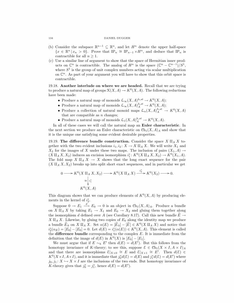
134 DANIEL DUGGER
(b) Consider the subspace Rn−1 ⊆ Rn, and let Hn denote the upper half-spacex ∈ Rn |xn > 0. Prove that IPn ∼= IPn−1×Hn, and deduce that IPn iscontractible for all n ≥ 1.
(c) Use a similar line of argument to show that the space of Hermitian inner prod-ucts on Cn is contractible. The analog of Hn is the space (Cn − Cn−1)/S1,where S1 is the group of unit complex numbers acting via scalar multiplicationon Cn. As part of your argument you will have to show that this orbit space iscontractible.
19.18. Another interlude on where we are headed. Recall that we are tryingto produce a natural map of groups K(X,A)→ K0(X,A). The following reductionshave been made:
• Produce a natural map of monoids L∞(X,A)h,st → K0(X,A);• Produce a natural map of monoids L∞(X,A)h,stA → K0(X,A);• Produce a collection of natural monoid maps Ln(X,A)h,stA → K0(X,A)
that are compatible as n changes;• Produce a natural map of monoids L1(X,A)h,stA → K0(X,A).
In all of these cases we will call the natural map an Euler characteristic. Inthe next section we produce an Euler characteristic on Ch1(X,A)A and show thatit is the unique one satisfying some evident desirable properties.
19.19. The difference bundle construction. Consider the space X qA X to-gether with the two evident inclusions i1, i2 : X → X qA X. We will write X1 andX2 for the images of X under these two maps. The inclusion of pairs (X1, A) →(X qAX,X2) induces an excision isomorphism i∗1 : K0(X qAX,X2)→ K0(X1, A).The fold map X qA X → X shows that the long exact sequence for the pair(X qA X,X2) breaks up into split short exact sequences, and in particular we get
0 // K0(X qA X,X2)
∼= i∗1
// K0(X qA X)i∗2 // K0(X2) // 0.
K0(X,A)
This diagram shows that we can produce elements of K0(X,A) by producing ele-ments in the kernel of i∗2.
Suppose 0 → E1d−→ E0 → 0 is an object in Ch1(X,A)A. Produce a bundle
on X qA X by taking E1 → X1 and E0 → X2 and gluing them together alongthe isomorphism d defined over A (see Corollary 8.17). Call this new bundle E →X qA X. Likewise, by gluing two copies of E0 along the identity map we producea bundle E 0 on X qA X. Set α(E) = [E 0] − [E ] ∈ K0(X qA X) and notice thati∗2(αE) = [E0]− [E0] = 0. Let d(E) = i∗1(α(E)) ∈ K0(X,A). This element is calledthe difference bundle corresponding to the complex E. It is immediate from thedefinition that the image of d(E) in K0(X) is [E0]− [E1].
We must argue that if E ∼h E′ then d(E) = d(E′). But this follows from thehomotopy invariance of K-theory; to see this, suppose E ∈ Ch1(X × I,A × I)Aand that there are isomorphisms E|X×0
∼= E and E|X×1∼= E′. Then d(E) ∈
K0(X×I,A×I), and it is immediate that j∗0d(E) = d(E) and j∗1d(E) = d(E′) wherej0, j1 : X → X × I are the inclusions of the two ends. But homotopy invariance ofK-theory gives that j∗0 = j∗1 , hence d(E) = d(E′).
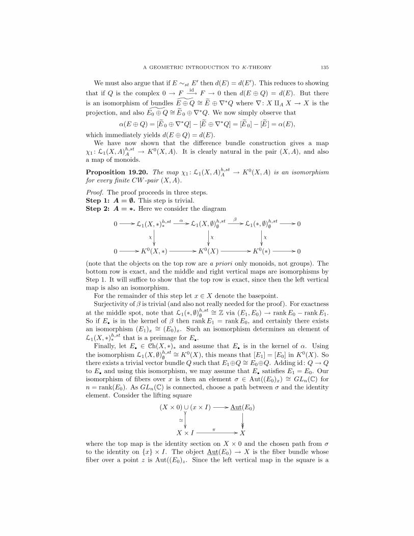
A GEOMETRIC INTRODUCTION TO K-THEORY 135
We must also argue that if E ∼st E′ then d(E) = d(E′). This reduces to showingthat if Q is the complex 0 → F
id−→ F → 0 then d(E ⊕ Q) = d(E). But thereis an isomorphism of bundles E ⊕Q ∼= E ⊕ ∇∗Q where ∇ : X qA X → X is theprojection, and also E0 ⊕Q ∼= E 0 ⊕∇∗Q. We now simply observe that
α(E ⊕Q) = [E 0 ⊕∇∗Q]− [E ⊕∇∗Q] = [E 0]− [E ] = α(E),
which immediately yields d(E ⊕Q) = d(E).We have now shown that the difference bundle construction gives a map
χ1 : L1(X,A)h,stA → K0(X,A). It is clearly natural in the pair (X,A), and alsoa map of monoids.
Proposition 19.20. The map χ1 : L1(X,A)h,stA → K0(X,A) is an isomorphismfor every finite CW -pair (X,A).
Proof. The proof proceeds in three steps.Step 1: A = ∅. This step is trivial.Step 2: A = ∗. Here we consider the diagram
0 // L1(X, ∗)h,st∗α //
χ
L1(X, ∅)h,st∅β //
χ
L1(∗, ∅)h,st∅
χ
// 0
0 // K0(X, ∗) // K0(X) // K0(∗) // 0
(note that the objects on the top row are a priori only monoids, not groups). Thebottom row is exact, and the middle and right vertical maps are isomorphisms byStep 1. It will suffice to show that the top row is exact, since then the left verticalmap is also an isomorphism.
For the remainder of this step let x ∈ X denote the basepoint.Surjectivity of β is trivial (and also not really needed for the proof). For exactness
at the middle spot, note that L1(∗, ∅)h,st∅∼= Z via (E1, E0) → rankE0 − rankE1.
So if E• is in the kernel of β then rankE1 = rankE0, and certainly there existsan isomorphism (E1)x ∼= (E0)x. Such an isomorphism determines an element ofL1(X, ∗)h,st∗ that is a preimage for E•.
Finally, let E• ∈ Ch(X, ∗)∗ and assume that E• is in the kernel of α. Usingthe isomorphism L1(X, ∅)h,st∅
∼= K0(X), this means that [E1] = [E0] in K0(X). Sothere exists a trivial vector bundle Q such that E1⊕Q ∼= E0⊕Q. Adding id: Q→ Qto E• and using this isomorphism, we may assume that E• satisfies E1 = E0. Ourisomorphism of fibers over x is then an element σ ∈ Aut((E0)x) ∼= GLn(C) forn = rank(E0). As GLn(C) is connected, choose a path between σ and the identityelement. Consider the lifting square
(X × 0) ∪ (x× I) //
'
Aut(E0)
X × I π // X
where the top map is the identity section on X × 0 and the chosen path from σto the identity on x × I. The object Aut(E0) → X is the fiber bundle whosefiber over a point z is Aut((E0)z. Since the left vertical map in the square is a
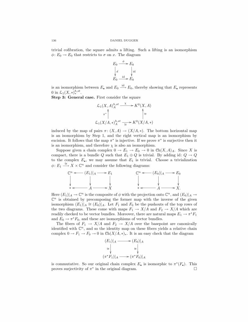
136 DANIEL DUGGER
trivial cofibration, the square admits a lifting. Such a lifting is an isomorphismφ : E0 → E0 that restricts to σ on x. The diagram
E0φ //
d
E0
id
E0
id // E0
is an isomorphism between E• and E0id−→ E0, thereby showing that E• represents
0 in L1(X, ∗)h,st∗ .Step 3: General case. First consider the square
L1(X,A)h,stA
χ // K0(X,A)
L1(X/A, ∗)h,stA
π∗
OO
∼=// K0(X/A, ∗)
∼=
OO
induced by the map of pairs π : (X,A) → (X/A, ∗). The bottom horizontal mapis an isomorphism by Step 1, and the right vertical map is an isomorphism byexcision. It follows that the map π∗ is injective. If we prove π∗ is surjective then itis an isomorphism, and therefore χ is also an isomorphism.
Suppose given a chain complex 0 → E1 → E0 → 0 in Ch(X,A)A. Since X iscompact, there is a bundle Q such that E1 ⊕ Q is trivial. By adding id: Q → Qto the complex E•, we may assume that E1 is trivial. Choose a trivializationφ : E1
∼=−→ X × Cn and consider the following diagrams:
Cn
(E1)|Aoo //
E1
Cn
(E0)|Aoo //
E0
∗ A //oo X ∗ A //oo X.
Here (E1)|A → Cn is the composite of φ with the projection onto Cn, and (E0)|A →Cn is obtained by precomposing the former map with the inverse of the givenisomorphism (E1)|A ∼= (E0)|A. Let F1 and F0 be the pushouts of the top rows ofthe two diagrams. These come with maps F1 → X/A and F2 → X/A which arereadily checked to be vector bundles. Moreover, there are natural maps E1 → π∗F1
and E0 → π∗F0, and these are isomorphisms of vector bundles.The fibers of F1 → X/A and F2 → X/A over the basepoint are canonically
identified with Cn, and so the identity map on these fibers yields a relative chaincomplex 0→ F1 → F0 → 0 in Ch(X/A, ∗)∗. It is an easy check that the diagram
(E1)|A∼=
// (E0)|A∼=
(π∗F1)|A // (π∗F0)|A
is commutative. So our original chain complex E• is isomorphic to π∗(F•). Thisproves surjectivity of π∗ in the original diagram.
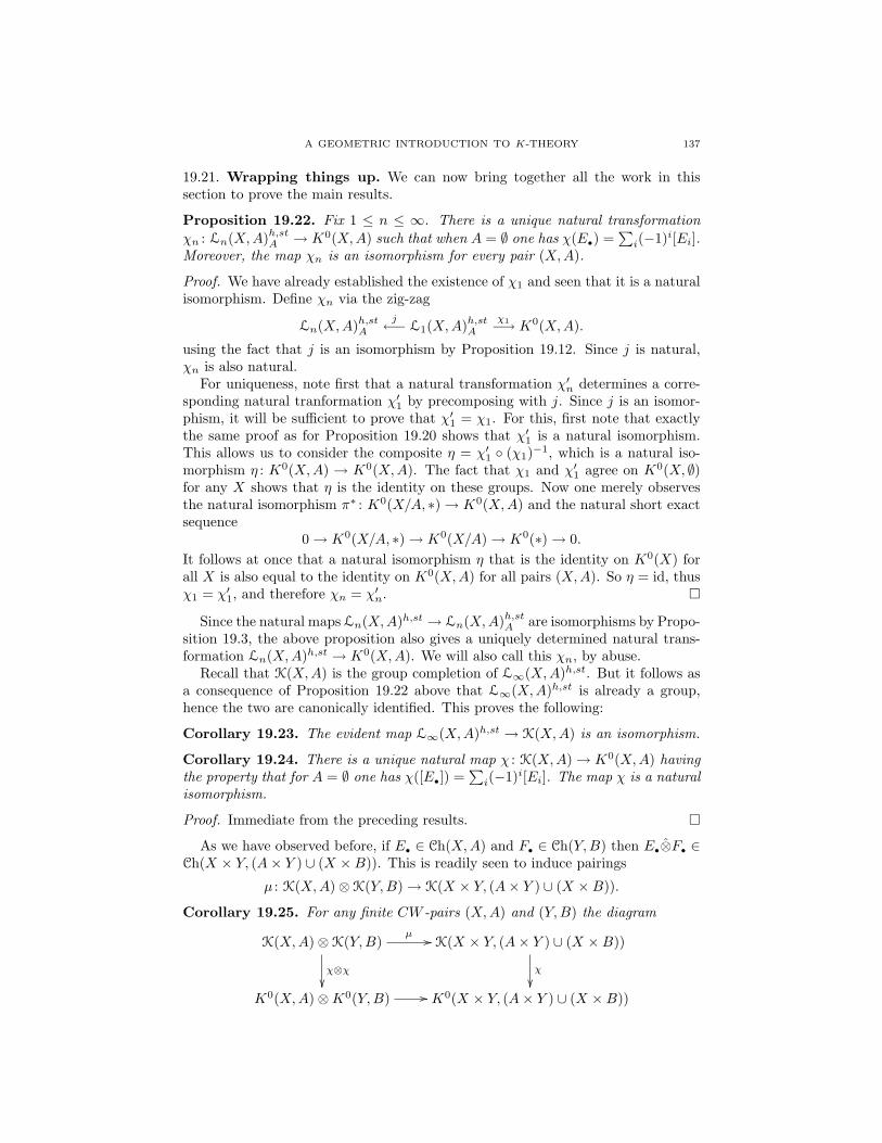
A GEOMETRIC INTRODUCTION TO K-THEORY 137
19.21. Wrapping things up. We can now bring together all the work in thissection to prove the main results.
Proposition 19.22. Fix 1 ≤ n ≤ ∞. There is a unique natural transformationχn : Ln(X,A)h,stA → K0(X,A) such that when A = ∅ one has χ(E•) =
∑i(−1)i[Ei].
Moreover, the map χn is an isomorphism for every pair (X,A).
Proof. We have already established the existence of χ1 and seen that it is a naturalisomorphism. Define χn via the zig-zag
Ln(X,A)h,stA
j←− L1(X,A)h,stA
χ1−→ K0(X,A).
using the fact that j is an isomorphism by Proposition 19.12. Since j is natural,χn is also natural.
For uniqueness, note first that a natural transformation χ′n determines a corre-sponding natural tranformation χ′1 by precomposing with j. Since j is an isomor-phism, it will be sufficient to prove that χ′1 = χ1. For this, first note that exactlythe same proof as for Proposition 19.20 shows that χ′1 is a natural isomorphism.This allows us to consider the composite η = χ′1 (χ1)−1, which is a natural iso-morphism η : K0(X,A) → K0(X,A). The fact that χ1 and χ′1 agree on K0(X, ∅)for any X shows that η is the identity on these groups. Now one merely observesthe natural isomorphism π∗ : K0(X/A, ∗)→ K0(X,A) and the natural short exactsequence
0→ K0(X/A, ∗)→ K0(X/A)→ K0(∗)→ 0.It follows at once that a natural isomorphism η that is the identity on K0(X) forall X is also equal to the identity on K0(X,A) for all pairs (X,A). So η = id, thusχ1 = χ′1, and therefore χn = χ′n.
Since the natural maps Ln(X,A)h,st → Ln(X,A)h,stA are isomorphisms by Propo-sition 19.3, the above proposition also gives a uniquely determined natural trans-formation Ln(X,A)h,st → K0(X,A). We will also call this χn, by abuse.
Recall that K(X,A) is the group completion of L∞(X,A)h,st. But it follows asa consequence of Proposition 19.22 above that L∞(X,A)h,st is already a group,hence the two are canonically identified. This proves the following:
Corollary 19.23. The evident map L∞(X,A)h,st → K(X,A) is an isomorphism.
Corollary 19.24. There is a unique natural map χ : K(X,A)→ K0(X,A) havingthe property that for A = ∅ one has χ([E•]) =
∑i(−1)i[Ei]. The map χ is a natural
isomorphism.
Proof. Immediate from the preceding results.
As we have observed before, if E• ∈ Ch(X,A) and F• ∈ Ch(Y,B) then E•⊗F• ∈Ch(X × Y, (A× Y ) ∪ (X ×B)). This is readily seen to induce pairings
µ : K(X,A)⊗K(Y,B)→ K(X × Y, (A× Y ) ∪ (X ×B)).
Corollary 19.25. For any finite CW -pairs (X,A) and (Y,B) the diagram
K(X,A)⊗K(Y,B)
χ⊗χ
µ // K(X × Y, (A× Y ) ∪ (X ×B))
χ
K0(X,A)⊗K0(Y,B) // K0(X × Y, (A× Y ) ∪ (X ×B))

138 DANIEL DUGGER
is commutative, where the bottom horizontal map is the product on K-theory.
Proof. It is trivial to check that the diagram commutes when A = B = ∅. Thegeneral case follows formally from this one using naturality. First check that itworks for A = B = ∗ using the diagram
K0(X, ∗)⊗K0(Y, ∗) //
∼=
K0(X × Y, (X × ∗) ∪ (∗ × Y ))**
**UUUUUUUUUUUUUUUK0(X ∧ Y, ∗)
∼=oo
K0(X)⊗K0(Y ) // K0(X × Y )
(and the similar one for K(−,−)). It is important that the indicated maps areinjections, but that they are so is an easy argument. Finally, deduce the generalcase using the diagrams
K0(X,A)⊗K0(Y,B) // K0(X × Y, (A× Y ) ∪ (X ×B)) K0(X/A ∧ Y/B, ∗)
∼=ttiiiiiiiiiiiiiiii
∼=oo
K0(X/A, ∗)⊗K0(Y/B, ∗)
∼=
OO
// K0(X/A× Y/B,X/A ∨ Y/B).
Finally, we note that the above results for finite CW -pairs (X,A) automaticallyextend to homotopically compact pairs. If (X,A) is homotopically compact thenchoose a finite CW -pair (X ′, A′) and a map (X ′, A′) → (X,A) that is a weakhomotopy equivalence on each factor. Define χ : K(X,A) → K0(X,A) via thediagram
K(X ′, A′)
∼=
K(X,A)∼=oo
K0(X ′, A′) K0(X,A).∼=
oo
A straightforward argument using Proposition 17.14 and Proposition C.3 showsthat this does not depend on the choice of (X ′, A′). Everything that we haveproven about K(−,−) → K0(−,−) for finite CW -pairs now immediately followsfor homotopically compact pairs as well.
Remark 19.26. Note that we have now proven Theorem 17.16, since that resultis just a compilation of Corollaries 19.24 and 19.25.
A GEOMETRIC INTRODUCTION TO K-THEORY 139
Part 4. K-theory and geometry II
In the last several sections we developed the basic connections between K-theoryand geometry. We have seen that K-theory is a complex-oriented cohomologytheory, and we understand “geometric” representatives for the Thom classes andfundamental classes that come with such a theory; in this case “geometric” meansthat we can write down explicit chain complexes of vector bundles representing theclasses. In the following sections our aim is to further explore this general area:now that the basic picture is in place, where does it take us? The topics we coverare somewhat of a hodgepodge, but in some sense they they all revolve around theexploration of fundamental classes.
20. K∗(CPn) and the K-theoretic analog of the degree
If Z → CPn is a complex submanifold then it has a fundamental class [Z]in H∗(CPn). Knowing this fundamental class comes down to knowing a singleinteger, called the degree of Z. The geometric interpretation of the degree is thatit equals the number of points of intersection between Z and a generically chosenlinear subspace of complementary dimension. In this section we will repeat thisline of investigation but replacing H∗ with K∗. So we must compute K∗(CPn)and investigate what information is encoded in the fundamental class [Z]K . Wewill find that knowing [Z]K amounts to knowing several integers (not just one);while we can give methods for computing these, their geometric interpretation issomewhat mysterious.
20.1. Calculation of K∗(CP n). We begin with the following easy lemma:
Lemma 20.2. Let E be any multiplicative cohomology theory. If x1, . . . , xn+1 ∈E∗(CPn), then x1 · · ·xn+1 = 0.
Proof. The key is just that CPn can be covered by n + 1 contractible sets. To beexplicit, let Ui = [z0 : . . . : zn] ∈ CPn | zi 6= 0. Then Ui is open in CPn and ishomeomorphic to Cn.
Choose our basepoint of CPn to be [1 : 1 : · · · : 1] (or any other point in theintersection of all the Ui’s). The contractibility of Ui implies that E∗(CPn, Ui)→E∗(CPn, ∗) is an isomorphism. So we may lift each xi to a class xi ∈ E∗(CPn, Ui).
It now follows that x1x2 · · · xn+1 lifts x1 . . . xn+1 in the map
E∗(CPn, U1 ∪ · · · ∪ Un+1)→ E∗(CPn, ∗).Since U1∪ · · ·∪Un+1 = CPn, the domain is the zero group. So x1 . . . xn+1 = 0.
Recall that H∗(CPn) ∼= Z[x]/(xn+1) where x is a generator in degree 2. It isnot hard to see that we may take x = [CPn−1]. This calculation works for anycomplex-oriented cohomology theory:
Proposition 20.3. Let E be a complex-oriented cohomology theory. There is anisomorphism of rings
E∗(pt)[x]/(xn+1)→ E∗(CPn)sending xi to [CPn−i].
140 DANIEL DUGGER
Proof. Consider the reduced Gysin sequence for the submanifold CPn−1 j→ CPn:
· · · Ek(CPn − CPn−1)oo Ek(CPn)oo
Ek−2(CPn−1)
j!
OO
Ek−1(CPn − CPn−1)oo · · ·oo
Let x = [CPn−1] = j!(1) ∈ E2(CPn). By Lemma 20.2 we know xn+1 = 0, sowe get a map E∗(pt)[x]/(xn+1) → E∗(CPn). We will show that this map is anisomorphism via induction on n. The case n = 0 is trivial.
Note that x2 = [CPn−2] by intersection theory, and more generally xi = [CPn−i].The spaces CPn − CPn−1 are homeomorphic to Cn and hence contractible.
So the reduced Gysin sequence considered above breaks up into a collection ofisomorphisms
j! : Ek−2(CPn−1)∼=−→ Ek(CPn).
Taking all k’s together, j! is a map of E∗(pt)-modules and therefore an isomorphismof such modules. By induction E∗(CPn−1) is a free E∗(pt)-module generated bythe classes 1 = [CPn−1], [CPn−2], [CPn−3], . . . , [CP 0]. Since the pushforward j!sends [CPn−i] to [CPn−i], we conclude that E∗(CPn) is a free E∗(pt)-module on[CPn−1], . . . , [CP 0]. If we add 1 to this collection then we get a free basis forE∗(CPn) over E∗(pt). This proves that our map E∗(pt)[x]/(xn+1) → E∗(CPn) isan isomorphism.
In the case of complex K-theory, we can rephrase the above result as sayingthat Kodd(CPn) = 0 and K0(CPn) = Z[X]/(Xn+1), where X = β · [CPn−1]. Inparticular, note that additively we have K0(CPn) ∼= Zn+1 with free basis consistingof the powers of X. Ignoring powers of the Bott element at usual, we can write thisfree basis as [CPn], [CPn−1], . . . , [CP 0].
20.4. Fundamental classes in K∗(CP n). Now let Z → CPn be a complex,closed submanifold of codimension c. Recall that if we consider fundamental classesin singular cohomology then we have [Z] = d · [CPn−c] for a unique integer d thatis called the degree of Z. Geometrically, d is the number of points on intersectionof Z with a generically chosen copy of CP c.
We can now play this same game in the context of K-theory. We have a funda-mental class [Z]K ∈ K0(CPn), and we can therefore write
[Z]K = d0 · [CPn] + d1 · [CPn−1] + · · ·+ dn[CP 0]
= d0 · 1 + d1X + d2X2 + · · ·+ dnX
n
for unique integers di. These integers are topological invariants of the embeddingZ → CPn; our goal will be to explore them further. Multiply the above equationby Xn to obtain
d0Xn = [Z]K ·Xn = [Z]K · [CP 0] = [Z ∩ CP 0]
where in the last term we mean the intersection of Z with a generically chosencopy of CP 0. But as long as Z is not all of CPn, this generic intersection willbe empty—so if Z is codimension at least one then d0 = 0. We then repeat thisargument, but multiplying by Xn−1 instead of Xn: we get
d1Xn = [Z]K · [CP 1] = [Z ∩ CP 1].
A GEOMETRIC INTRODUCTION TO K-THEORY 141
Again, if the codimension of Z is at least 2 then the CP 1 can be moved so that itdoesn’t intersect Z at all, hence d1 = 0. Continuing this argument we find that
0 = d0 = d1 = · · · = dc−1 and dc = deg(Z).
The last equality follows because Z intersects a generic CP c in deg(Z) many points.The situation can be summarized as follows: the first non-vanishing di coincideswith the classical degree of Z, but there is the possibility of the higher di’s beingnonzero. This is what we will investigate next.
Remark 20.5. Notice that what we have done so far works in any complex-orientedcohomology theory E∗. The fundamental class [Z] can be written as a linear com-bination of the classes [CPn−i] with coefficients from E∗(pt). The first c of thesecoefficients vanish, until one gets to the coefficient of [CPn−c]—which must be equalto deg(Z). After this things become interesting, in the sense that one has invariantsthat are not detected in singular cohomology.
To proceed further with our analysis of the higher di’s in K-theory, we need toconnect our fundamental classes with the vector bundle description of K-theory:
Lemma 20.6. In K0(CPn) one has [CPn−1] = 1 − L where L → CPn is thetautological line bundle. Consequently, [CPn−k] = (1− L)k for all k.
Proof. We give two explanations. For the first, consider the map of vector bundlesf : L → 1 defined as follows: in the fiber over x = [x0 : x1 : · · · : xn] we send(x0, . . . , xn) to x0. Note that this is well-defined, since multiplying all the xi’s bya scalar λ yields the same homomorphism Lx → C.
The map f is exact on all fibers except those where x0 = 0. The complex0 → L → 1 → 0 is a resolution of the structure sheaf for CPn−1, and hence 1− Lrepresents the associated fundamental class in K-theory by Theorem 18.8.
Our second explanation takes place entirely in the topological world. The keyfact is that the normal bundle to CPn−1 inside CPn is L∗. Let U be a tubularneighborhood of CPn−1, and consider the chain of isomorphisms
K0(CPn,CPn − CPn−1)∼=−→ K0(U,U − CPn−1) ∼= K0(N,N − 0).
The relative fundamental class [CPn−1]rel is the unique class that maps to theThom class UN under the above isomorphisms. But N is a line bundle, and recallthat the Thom class is then [J∗] = [π∗N∗ → 1] where π : N → CPn−1. A littlethought shows that the complex 0 → π∗N∗ → 1 → 0 is exactly the restrictionof 0 → L → 1 → 0 on CPn. So this latter complex represents [CPn−1]rel, andtherefore 1− L equals [CPn−1].
Example 20.7. Note that it follows from the above lemma that (1 − L)n+1 = 0in K0(CPn). This relation comes up in many contexts, and it is useful to have adifferent perspective on it. Let R = C[x0, . . . , xn] and consider the Koszul complexfor the regular sequence x0, . . . , xn. It has the form
0→ R(−n− 1)→ · · · → R(−2)(n+1
2 ) → R(−1)n+1 → R→ 0,
and we know this complex is exact. It therefore gives a corresponding exact se-quence of vector bundles on CPn, which tells us that
0 = 1− (n+ 1)L+(n+1
2
)L2 − · · ·+ (−1)n+1Ln+1
in K0(CPn). Of course the expression on the right is precisely (1− L)n+1.
142 DANIEL DUGGER
We next compute the K-theoretic fundamental classes in a couple of simpleexamples:
Example 20.8. Let Z = V (f) → CPn be a smooth hypersurface of degree d. LetR = C[x0, . . . , xn]. The coordinate ring of Z is R/(f), which has the short freeresolution given by
0→ R(−d) ·f−→ R→ R/(f)→ 0.So [Z] = 1−Ld in K0(CPn). To write [Z] as a linear combination of the [CPn−i]’swe need to write 1− Ld in terms of powers of 1− L. This is easy, of course:
[Z] = 1− Ld = 1− [1− (1− L)]d = 1− (1−X)d
= 1− [1− dX +(d2
)X2 − · · ·+ (−1)dXd]
= dX −(d2
)X2 +
(d3
)X3 − · · ·
So we find that the higher di’s for a hypersurface are all just (up to sign) binomialcoefficients of d. This is somewhat disappointing, as we are not seeing new topolog-ical invariants—it is just the degree over and over again, encoded in different ways.[This is not actually not a surprise: the degree is known to be the only topologicalinvariant for embedded hypersurfaces].
Things become more interesting in the next example:
Example 20.9. Consider Z = V (f, g) where f, g is a regular sequence of homoge-neous elements in R = C[x0, . . . , xn]. Let d = deg(g) and e = deg(g). Because f, gis a regular sequence, R/(f, g) is resolved by the Koszul complex:
0→ R(−d− e)→ R(−d)⊕R(−e)→ R→ R/(f, g)→ 0.
We can now calculate
[Z]K =[
0 // Ld+e // Ld ⊕ Le // 1 // 0]
= 1− (Ld + Le) + Ld+e
= 1− (1−X)d − (1−X)e + (1−X)d+e
=[(d+e2
)−(d2
)−(e2
)]X2 −
[(d+e3
)−(d3
)−(e3
)]X3 + · · ·
= deX2 + 12de(2− d− e)X
3 + . . . .
The classical degree of Z is de, but our ‘higher invariants’ now see more than justthis number. In fact, knowing the expansion of [Z]K as a linear combination of theXi’s implies that we know de and de(2−d−e), which implies that we know d+e. Butif we know de and d+e then we know the polynomial (ξ−d)(ξ−e) = ξ2−(d+e)ξ+de,which means we know its roots. So knowing the expansion of [Z]K is the same asknowing d and e. This example shows that the K-theoretic fundamental class seesmore topological information than the singular cohomology fundamental class does.
Now that we have seen these simple examples we can return to our main question.Given Z → CPn of codimension c, how does one compute the di’s in the equation
[Z]K = (degZ)[CPn−c] + dc+1[CPn−c−1] + dc+2[CPn−c−2] + · · ·And what do these di’s mean in terms of geometry? We will soon see that oneanswer is given by the Hilbert polynomial.
A GEOMETRIC INTRODUCTION TO K-THEORY 143
20.10. Review of the Hilbert polynomial. Let R = C[x0, . . . , xn], and regardthis as a graded ring where each xi has degree one. If M is a graded R-modulewrite Ms for the graded piece in degree s. The Poincare series of M is the formalpower series
PM (ξ) =∞∑
s=−∞(dimMs)ξs ∈ Z[[ξ]]
(defined if M is finitely-generated over R). Note that this is evidently an additiveinvariant of finitely-generated, graded modules: if 0 → M ′ → M → M ′′ → 0 is anexact sequence then clearly PM (ξ) = PM ′(ξ) + PM ′′(ξ). We may therefore regardthe Poincare series as a map of abelian groups
P : Ggrd(R)→ Z[[ξ]]
where Ggrd(R) is the Grothendieck group of finitely-generated graded modules overR.
We will calculate the Poincare series of each R(−k), but for this we need thefollowing useful calculation:
Lemma 20.11. The number of monomials of degree d in the variables z1, . . . , znis equal to
(d+n−1
d
).
Proof. Monomials are in bijective correspondence with patterns of “dashes andslashes” that look like
−−−/−−//−−−−/− .The above pattern corresponds to the monomial z3
1z22z
44z5, and from this the general
form of the bijection should be clear. Monomials of degree d will correspond topatterns with d dashes, and if there are n variables then there will be n−1 slashes.So we need to count patterns where there will be d+ n− 1 total symbols, of whichd are dashes: the number of these is
(d+n−1
d
).
It is an immediate consequence that PR(ξ) =∑s≥0
(s+nn
)ξs. For R(−k) we
simply shift the coefficients and obtain
PR(−k)(ξ) =∑s≥k
(s+n−kn
)ξs = ξkPR(ξ).
The power series ξkPR(ξ) | k ∈ Z are obviously linearly independent over Q, whichshows that Ggrd(R) has infinite rank as an abelian group.
Proposition 20.12. Ggrd(R) is isomorphic to Z∞, with free basis the set of rankone, free modules [R(−d) | d ∈ Z.
Proof. The key is the Hilbert Syzygy Theorem. Consider the diagram
Z∞ //
$$HHHHHHHHH Ggrd(R)
P
Z[[ξ]]
where the horizontal map sends the ith basis element to [R(−i)] and the diagonalmap is the composite. We have already seen that this composite is injective, becausethere is no Z-linear relation amongst the images of the basis elements. So Z∞ →Ggrd(R) is injective, and it only remains to prove surjectivity. But if M is any
144 DANIEL DUGGER
finitely-generated, graded R-module then the Syzygy Theorem guarantees a finite,graded, free resolution
0→ Fn → Fn−1 → · · · → F1 → F0 →M → 0.
So [M ] =∑i(−1)i[Fi], and each Fi is a sum of elements [R(−k)]. This proves
surjectivity.
The Hilbert polynomial is a variant of the Poincare series that keeps track ofless information. At first this might seem to be a bad thing, but we will see thatwhat it does is give us a closer connection to geometry and topology. Here is themain result that gets things started:
Proposition 20.13. Let M be a finitely-generated module M over R. Then thereexists a unique polynomial HM (s) ∈ Q[s] that agrees with the function s 7→ dimMs
for s 0. One has degHM (s) ≤ n. The polynomial HM (s) is called the Hilbertpolynomial of M .
Proof. Consider first the case M = R. A basis for Ms consists of all monomials inx0, . . . , xn of degree s, which Lemma 20.11 calculates to be
(n+ss
)=(n+sn
). This is
a polynomial in s of degree n. Next consider M = R(−k). The function s 7→ Ms
is zero for s < k, and then for s ≥ k it coincides with(n+s−kn
). This is again a
polynomial in s of degree n.Finally, consider the case of a general M . By the Hilbert Syzygy Theorem M
has a finite, graded, free resolution
0→ Fn → Fn−1 → · · · → F1 → F0 →M → 0.
It follows that
dimMs = dim(F0)s − dim(F1)s + · · ·+ (−1)n dim(Fn)s.
But each Fi is a direct sum of finitely-many R(−k)’s, and so s 7→ dim(Fi)s hasbeen shown to agree with a polynomial in s of degree at most n, for s 0. Thedesired result follows at once.
The following calculation was given in the above proof, but we record it belowbecause it comes up so often:
Corollary 20.14. When R = C[x0, . . . , xn] and k ∈ Z the Hilbert polynomial forR(−k) is
(s+n−kn
).
Example 20.15. Consider a hypersurface M = R/(f), where f ∈ R is homoge-neous of degree d. We then have the resolution
0 // R(−d)·f // R // R/(f) // 0
from which we find
HR/(f) = HR −HR(−d) =(s+nn
)−(s+n−dn
)= (s+n)...(s+1)
n! − (s+n−d)...(s−d+1)n! .
Note that the two binomial coefficients have leading terms sn/n!, which thereforecancel. The coefficient of sn−1 is
1n! ·[n(n+1)
2 − (n−2d+1)n2
]= d
(n−1)! .
Note that the degree of HR/(f) is one less than the Krull dimension of R/(f), andthe leading coefficient is the degree of f (the geometric degree of the hypersurface)

A GEOMETRIC INTRODUCTION TO K-THEORY 145
divided by n!. These are general facts that hold for any module: the degree ofHM isone less than the Krull dimension of M , and the leading coefficient times (degHM )!is always an integer—this integer is called the multiplicity of the module M .Proofs can be found in most commutative algebra texts.
The Hilbert polynomial is an additive invariant of finitely-generated modules: if0 → M ′ → M → M ′′ → 0 is an exact sequence then clearly HM (s) = HM ′(s) +HM ′′(s). We may therefore regard the Hilbert polynomial as a map of abeliangroups
Hilb: Ggrd(R)→ Q[s].This map is clearly not injective, however: it kills any module that is finite-dimensional as a C-vector space. The subgroup of Ggrd(R) generated by suchmodules is A = 〈[C(−d)] | d ∈ Z〉. We may regard Hilb as a map
Hilb: Ggrd(R)/A→ Q[s].
The domain of this map is calculated as follows:
Proposition 20.16. The group Ggrd(R)/A is isomorphic to Zn+1, with free basisR,R(−1), R(−2), . . . , R(−n). The map Hilb is an injection.
Proof. Let B be the subgroup of Ggrd(R)/A generated by [R], [R(−1)], . . . , [R(−n)].We will show that B is equal to the whole group.
The module C is resolved by the Koszul complex K(x0, . . . , xn;R). This givesthe relation in Ggrd(R) of
[C] = [R]− (n+ 1)[R(−1)] +(n+1
2
)[R(−2)] + · · ·+ (−1)n+1[R(−n− 1)].
In Ggrd(R)/A we therefore have [R(−n − 1)] ∈ B. For d > 0 we can tensorthe Koszul complex with R(−d) and then apply the same argument to find that[R(−n − 1 − d)] ∈ 〈[R], [R(−1)], . . . , R(−n − d)]〉. By induction we therefore havethat [R(−k)] ∈ B for every k ≥ n+ 1.
A similar induction works for d < 0 to show that [R(−d)] ∈ B for all d ∈ Z. Inother words, B = Ggrd(R)/A.
Now consider the map Zn+1 → Ggrd(R)/A that sends the ith basis element eito [R(−i)] for 0 ≤ i ≤ n. We have just shown that this map is surjective. Consider,then, the composite
Zn+1 −→ Ggrd(R)/A Hilb−→ Q[s].The images of our basis elements are the polynomials(
s+nn
),(s+n−1n
),(s+n−2n
), . . . ,
(sn
).
Evaluating these polynomials at s = 0 gives the sequence 1, 0, 0, . . . , 0. Evaluatingat s = 1 gives n + 1, 1, 0, 0, . . . , 0, and so forth. For s = i the ith polynomialin the list evaluates to 1 and all the subsequent polynomials evaluate to 0. Thisproves that these polynomials are linearly independent over Z, hence the abovecomposite map is injective. So Zn+1 → Ggrd(R)/A is injective, and therefore is anisomorphism. Moreover, Hilb is injective.
The reader might notice that the Zn+1 in the above result is really ‘the same’ asthe group K0(CPn). This is the basis for what we do in the next section.

146 DANIEL DUGGER
Example 20.17. We will not need this, but it is a cute fact: Prove that the imageof Hilb : G(R)/A → Q[s] equals the set of polynomials f(s) ∈ Q[s] having theproperty that f(Z) ⊆ Z. That is, the image consists of all rational polynomialsthat take integer values on integers.
20.18. K-theory and the Hilbert polynomial. We now explain how the Hilbertpolynomial encodes the same information as the K-theoretic fundamental class.
Given Z → CPn a smooth subvariety of codimension c, recall that we have thefundamental class [Z] ∈ K0(CPn) and that we may write
[Z] = dc[CPn−c] + dc+1[CPn−c−1] + · · ·+ dn[CP 0].
We know that dc = deg(Z), and our goal is to understand how to compute thehigher di’s.
Recall that K0(CPn) is spanned by the classes [CPn−k] = (1 − L)k for k =0, 1, . . . , n. Evidently one can also use the basis 1, L, L2, . . . , Ln. We next introducean algebraic analogue of K0(CPn). Let R = C[x0, . . . , xn]. Take the Grothendieckgroup K0
grd(R) of finitely-generated, graded, projective R-modules (or equivalently,chain complexes of such modules) and quotient by the subgroup A generated by allcomplexes K(x0, . . . , xn;R)⊗R(−d) for d ∈ Z. We obtain a diagram
K0grd(R)/A
φ
∼=//
∼=
K0(CPn)
Ggrd(R)/A // Hilb // Q[s]
(20.19)
where the vertical map is our usual ‘Poincare Duality’ isomorphism and φ sends[R(−d)] to Ld. The map φ is an isomorphism by inspection: we have computedGgrd(R)/A and K0(CPn), both are Zn+1, and φ clearly maps a basis to a basis.
Given Z = V (I), we know that its fundamental class [Z] ∈ K0(CPn) is repre-sented by a finite, free resolution F• → R/I → 0. This resolution (or the alternatingsum of its terms) lifts to K0
grd(R)/A, and pushing this around the diagram into Q[s]just gives us HilbR/I(s). So the above diagram shows that knowing HilbR/I(s) isthe same as knowing [Z].
To say something more specific here, consider first the case Z = CPn−k. ThenR/I = R/(x0, . . . , xk−1), which as a graded ring is just C[xk, . . . , xn]. The Hilbertpolynomial is then
HilbCPn−k(s) =(s+n−kn−k
).
So pushing our basis [CPn], [CPn−1], . . . , [CP 0] around diagram (20.19) into Q[s]yields the polynomials (
s+nn
),(s+n−1n−1
),(s+n−2n−2
), . . . ,
(s0
).
If Z = V (I) → CPn is now arbitrary, then writing
HilbR/I(s) = d0
(s+nn
)+ d1
(s+n−1n−1
)+ d2
(s+n−2n−2
)+ . . .
implies that [Z] = d0[CPn] + d1[CPn−1] + d2[CPn−2] + . . . . In other words, oneobtains the expansion of [Z] as a linear combination of the [CPn−i]’s by writingHilbZ(s) as a linear combination of the above-listed binomial functions.

A GEOMETRIC INTRODUCTION TO K-THEORY 147
We have shown how to calculate the di’s from the ideal I of equations defin-ing Z: decompose the Hilbert polynomial into a sum of terms
(s+n−kk
), and take
the resulting coefficients. This is still not exactly a ‘geometric’ description of thedi’s, although it is a description that takes place in the domain of algebraic ge-ometry. We will get another perspective on this material via the Todd genus andthe Grothendieck-Riemann-Roch Theorem, studied in Section 25. See especiallySection 25.28.
21. Interlude on the calculus of finite differences
If f ∈ Q[t] let ∆f be the polynomial given by
(∆f)(t) = f(t+ 1)− f(t).
For example, ∆(t2) = (t+1)2− t2 = 2t+1, and ∆(t3) = (t+1)3− t3 = 3t2 +3t+1.Note that ∆: Q[t] → Q[t] is a linear map, and that it lowers degrees by one. Wecall ∆ the finite difference operator, and we regard it as an analog of the familiardifferentiation operator D : Q[t]→ Q[t].
The opposite of differentiation is integration, and there is an analogous operatorthat is the opposite of ∆. If f ∈ Q[t] define Sf to be the function given by
(Sf)(t) = f(0) + f(1) + f(2) + · · ·+ f(t− 1).
For example,S(t) = 0 + 1 + 2 + · · ·+ (t− 1) =
(t2
)= t(t−1)
2
andS(t2) = 02 + 12 + · · ·+ (t− 1)2 = (t−1)t(2t−1)
6 .
One should think of the formula for S(t) has giving a finite Riemann sum, based onintervals of width 1. It is not immediately clear that Sf is always a polynomial, northat it raises degrees by one, but we will prove these things shortly. The followingtwo facts are easy, though:
∆S(f) = f D∫
(f) = f
S∆(f) = f − f(0)∫D(f) = f − f(0).
We have written each identity paired with the corresponding identity for classicaldifferentiation/integration. Note that, like the usual integral, Sf will always be apolynomial that has zero as its constant term, since (Sf)(0) = 0 by definition.
Derivatives and integrals of polynomials are easy to compute because their val-ues on the basic polynomials tn are very simple. In fact, the point is really thatoperators D and
∫act very simply on the sequence of polynomials
1, t, t2
2 ,t3
3! ,t4
4! , . . .
Of course D carries each polynomial in the sequence to the preceding one, and∫
carries each polynomial to the subsequent one. In contrast, the operators ∆ and Sare not very well-behaved on this sequence. It is better to use the sequence
1, S(1), S2(1), S3(1), . . .
so let us compute these. It is easy to see that S(1) = t, and we previously saw thatS2(1) = S(t) =
(t2
). It follows from the following useful lemma that Sk(1) =
(tk
),
where the binomial coefficient stands for the polynomial 1k! t(t−1)(t−2) · · · (t−k+1).
148 DANIEL DUGGER
Lemma 21.1. For any d, k ∈ Z one has
∆(t+dk
)=(t+dk−1
), S
(tk
)=(t
k+1
).
Proof. The statement about ∆ follows from Pascal’s Identity. The statement aboutS is the identity (
0k
)+(1k
)+ · · ·+
(t−1k
)=(t
k+1
).
To prove this, imagine t slots labelled 1−−t where we are to place k+ 1 asterisks:
∗ ∗ ∗ ∗If the leftmost asterisk is in spot i, there are
(t−ik
)ways to place the remaining
asterisks. Summing over i ∈ [1, t] yields the desired formula.
The sequence of polynomials
1 =(t0
),(t1
),(t2
),(t3
), . . .
is clearly a basis for Q[t], as the kth term has degree equal to k. In relation to the∆ and S operators, this basis plays the role classically taken by the polynomials td
d! .It is now clear that S applied to a polynomial of degree d yields a polynomial ofdegree d+ 1: a polynomial of degree d is a linear combination of
(td
),(t
d−1
), . . . ,
(t0
)with the coefficient on the first term nonzero. Applying S changes each
(tk
)to(
tk+1
), and it is clear that this yields a polynomial of degree d+ 1.
For another example of the use of this binomial basis, note the following analogof the Taylor–Maclaurin explansion for writing polynomials in this basis:
Proposition 21.2. Let f ∈ Q[t]. Then
f =∞∑k=0
(∆kf)(0) ·(tk
).
Proof. We know f =∑Nk=0 ak
(tk
)for some N and some values ak ∈ Q. Plugging in
t = 0 immediately gives f(0) = a0. Now apply ∆ to get ∆f =∑N=1k=0 ak+1
(tk
)and
again plug in t = 0: this yields (∆f)(0) = a1. Continue.
Exercise 21.3. Let Q[t]int ⊆ Q[t] be the set of all polynomials f(t) such thatf(Z) ⊆ Z. Note that Q[t]int is stable under ∆ and S, and use this to prove thatQ[t]int is the Z-linear span of the polynomials
(tk
), k ≥ 0.
In contrast to the large number of similarities of the pair of operators (∆, S)to (D,
∫), there is an important difference when it comes to the product rule. Of
course we have D(fg) = (Df)g+ f(Dg), but one readily checks that this does notwork for ∆. The correct rule is as follows:
Lemma 21.4. For any f, g ∈ Q[t] one has ∆(fg) = (∆f)g + f(∆g) + (∆f)(∆g).
Proof. A simple calculation, left to the reader.
In the present section we will not have much use for this product rule, but itis a very important formula whose significance will become larger in subsequentsections.
A GEOMETRIC INTRODUCTION TO K-THEORY 149
21.5. Translating between (∆, S) and (D,∫
). If f ∈ Q[t] and h is any integer(or even better, a formal variable) we have the Taylor fomula
f(t+ h) =∞∑k=0
f (k)(t) · hk
k! =∞∑k=0
(Dkf)(t) · hk
k! .
Note that the sum is really finite, since large enough derivatives of f are all zero.Taking h = 1 and rearranging somewhat we get
f(t+ 1) =( ∞∑k=0
Dk
k!
)f = (eD)f.
Let us be clear about what this means. The expression∑∞k=0
Dk
k! makes perfectsense as an operator , since evaluating this at any fixed polynomial gives a well-defined answer. It is sensible to denote this operator as eD.
Taking one more step, we can write (∆f)(t) = f(t+1)− f(t) = (eD−1)f where1 denotes the identity operator. Or even more compactly,
∆ = eD − 1
is an identity of operators on Q[t]. This identity gives us ∆ as a linear combinationof iterates of D.
We are next going to cook up a similar formula for the operator S, but this isa little harder. One does not wish for a formula using higher and higher powersof∫
, as these operators become more and more complicated. Instead, we say toourselves that S is very close to being an inverse for D (it is a right inverse, butnot a left inverse). If it were an inverse we might want to write S = 1
eD−1, but it is
difficult to make sense of the latter expression as an operator—the trouble is thateD − 1 has no constant term, otherwise we could expand as a power series. Whilethis didn’t work, we can make sense of the operator
B = DeD−1
.(21.6)
By this we mean write xex−1 =
∑akx
k = 1− x2 + x2
12 − · · · as a formal power series,and set B equal to
∑∞k=0 akD
k. It follows purely formally that ∆Bf = Df for anypolynomial f , and therefore that
Bf − (Bf)(0) = SDf
(because S(Df) will not have a constant term). Replacing f by∫f in the above
formula, we getSf = SD(
∫f) = B(
∫f)− (B
∫f)(0).
Note that B(∫f) is equal to
∫f − 1
2f + 112Df − · · · . So this is as computable as
the series xex−1 ; the coefficients of this series are related to the Bernoulli numbers
(see Appendix A). We have
B =∞∑k=0
Bk
k! Dk
where the Bk’s are the Benoulli numbers.

150 DANIEL DUGGER
21.7. Sums of powers and Bernoulli numbers. The (∆, S) pair of operatorsis useful in a variety of mathematical situations. In a moment we will see anapplication to determining K-theoretic fundamental classes, but let us first look ata non-topological example. Almost every math student has seen the formulas
1 + 2 + · · ·+ n = n(n+1)2 and 12 + 22 + · · ·+ n2 = n(n+1)(2n+1)
6 .
The proof of such formulas by mathematical induction is a common exercise inelementary proof courses. It turns out that there are also formulas for higherpowers, of the form
1k + 2k + · · ·+ nk = pk(n)where pk(n) is a polynomial of degree k+1. How does one discover the appropriatepolynomials? This seems to have first been done by Jacob Bernoulli, the coefficientsin these polynomials being closely related to what are now called Bernoulli numbers.
Clearly we may rephrase the problem as that of computing S(tk), the exactconnection being S(tk) = pk(t− 1). In the last section we developed a formula forS in terms of the usual derivative and integral operators, and we will now use that;but here it is easiest to use it in the form
SD(f) = Bf−(Bf)(0) =
( ∞∑j=0
Bj
j! Dj
)f−(constant term of preceding expression).
We obtain
S(tk) = SD(tk+1
k+1
)= 1
k+1
∞∑j=0
Bj
j! Dj(tk+1)− (constant term)
= 1k+1
k∑j=0
Bj
j! (k + 1)(k)(k − 1) · · · (k + 2− j)tk+1−j
= 1k+1
k∑j=0
Bj ·(k+1j
)tk+1−j .
Note that the last expression is a polynomial in t, with all of its coefficients clearlyvisible.
Finally, recalling that S(tk) = pk(t− 1) we conclude that
1k + 2k + · · ·+ nk = 1k+1
k∑j=0
Bj ·(k+1j
)(n+ 1)k+1−j .
Exercise 21.8. Check that the above formula gives the familiar identities in thecases k = 1 and k = 2, and then see what it gives when k = 3. Compare the aboveformula to (A.3).
21.9. Back to K-theoretic fundamental classes. Let Z → CPn be a smoothhypersurface defined by the homogeneous ideal I ⊆ C[x0, . . . , xn]. We saw in Sec-tion 20.18 that the coefficients in
[Z]K = a0[CP 0]K + a1[CP 1]K + a2[CP 2]K + · · ·are the same as the coefficients in
HilbZ(t) = a0
(n+tn
)+ a1
(n+t−1n−1
)+ a2
(n+t−2n−2
)+ · · ·(21.10)
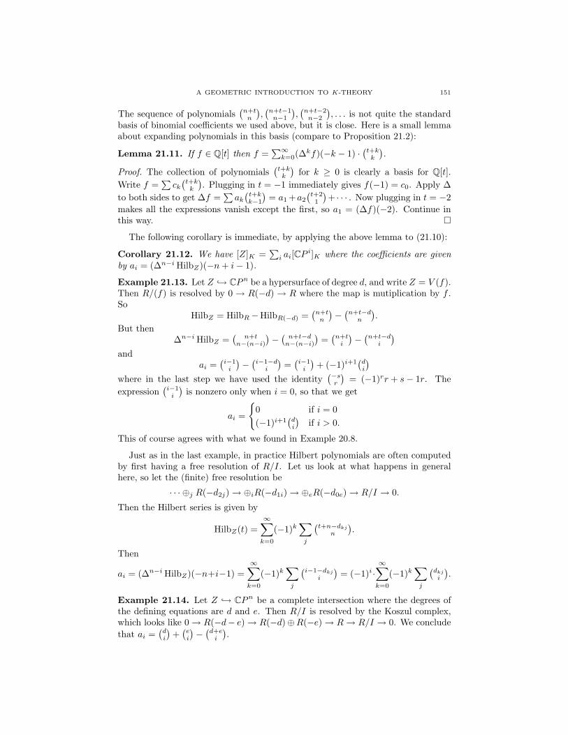
A GEOMETRIC INTRODUCTION TO K-THEORY 151
The sequence of polynomials(n+tn
),(n+t−1n−1
),(n+t−2n−2
), . . . is not quite the standard
basis of binomial coefficients we used above, but it is close. Here is a small lemmaabout expanding polynomials in this basis (compare to Proposition 21.2):
Lemma 21.11. If f ∈ Q[t] then f =∑∞k=0(∆
kf)(−k − 1) ·(t+kk
).
Proof. The collection of polynomials(t+kk
)for k ≥ 0 is clearly a basis for Q[t].
Write f =∑ck(t+kk
). Plugging in t = −1 immediately gives f(−1) = c0. Apply ∆
to both sides to get ∆f =∑ak(t+kk−1
)= a1 +a2
(t+21
)+ · · · . Now plugging in t = −2
makes all the expressions vanish except the first, so a1 = (∆f)(−2). Continue inthis way.
The following corollary is immediate, by applying the above lemma to (21.10):
Corollary 21.12. We have [Z]K =∑i ai[CP
i]K where the coefficients are givenby ai = (∆n−i HilbZ)(−n+ i− 1).
Example 21.13. Let Z → CPn be a hypersurface of degree d, and write Z = V (f).Then R/(f) is resolved by 0 → R(−d) → R where the map is mutiplication by f .So
HilbZ = HilbR−HilbR(−d) =(n+tn
)−(n+t−dn
).
But then∆n−i HilbZ =
(n+t
n−(n−i))−(n+t−dn−(n−i)
)=(n+ti
)−(n+t−d
i
)and
ai =(i−1i
)−(i−1−di
)=(i−1i
)+ (−1)i+1
(di
)where in the last step we have used the identity
(−sr
)= (−1)rr + s− 1r. The
expression(i−1i
)is nonzero only when i = 0, so that we get
ai =
0 if i = 0(−1)i+1
(di
)if i > 0.
This of course agrees with what we found in Example 20.8.
Just as in the last example, in practice Hilbert polynomials are often computedby first having a free resolution of R/I. Let us look at what happens in generalhere, so let the (finite) free resolution be
· · · ⊕j R(−d2j)→ ⊕iR(−d1i)→ ⊕eR(−d0e)→ R/I → 0.
Then the Hilbert series is given by
HilbZ(t) =∞∑k=0
(−1)k∑j
(t+n−dkj
n
).
Then
ai = (∆n−i HilbZ)(−n+i−1) =∞∑k=0
(−1)k∑j
(i−1−dkj
i
)= (−1)i ·
∞∑k=0
(−1)k∑j
(dkj
i
).
Example 21.14. Let Z → CPn be a complete intersection where the degrees ofthe defining equations are d and e. Then R/I is resolved by the Koszul complex,which looks like 0→ R(−d− e)→ R(−d)⊕R(−e)→ R→ R/I → 0. We concludethat ai =
(di
)+(ei
)−(d+ei
).

152 DANIEL DUGGER
Recall that if the codimension of Z → CPn is equal to c then we have ai = 0for i < c and ac = deg(Z). So any free resolution of R/I must satisfy the identities∑
k
(−1)k∑j
(dkj
i
)=
0 for i < c
deg(Z) for i = c.
In this way we obtain topological conditions on what free resolutions can look like.
Example 21.15. Show that the above conditions on the free resolution are equiv-alent to ∑
k
(−1)k∑j
dikj =
0 for i < c
deg(Z) · i! for i = c.
21.16. A digression on the Riemann zeta function. If Z → CPn then thevalues of the polynomial HilbZ(t) only have an a priori significance for t 0; recallthat these values represent the dimensions of the graded pieces of the coordinate ringof Z. Yet, we saw in Corollary 21.12 that the values of HilbZ(t) at certain negativeintegers (encoded as the value of a particular finite difference ∆? HilbZ) are equal tosome naturally-occurring topological invariants of Z. The fact that these negativevalues have any significance at all is a bit surprising. This situation is somewhatreminiscent of one involving the Riemann zeta function, that coincidentally (or not)is also related to the story of the (∆, S) operators. We are going to take a momentand talk about this, because of the feeling that it might be related to topology ina way that no one really understands yet.
Recall that Riemann’s ζ(s) is defined for Re(s) > 1 by the formula
ζ(s) =∞∑n=1
n−s.
Standard results from analysis show that this sum converges for Re(s) > 1, anddefines an analytic function in that range. It is a non-obvious fact that ζ(s) canbe analytically continued to the punctured plane C− 1. The values on negativenumbers turn out to be computable and are related to the Bernoulli numbers. Wewill give an entirely non-rigorous treatment of this computation; despite its failureto actually make sense, it is nevertheless somewhat intriguing.
If f ∈ Q[t] then we have seen that eDf makes sense and is equal to the polynomialf(t+ 1). It readily follows that enDf = f(t+ n) for any integer n ≥ 0. Now write
f(t) + f(t+ 1) + f(t+ 2) + · · · = [I + eD + e2D + e3D + · · · ]f =[
1I−eD
]f.
Of course none of the terms in the above identities make any sense, but let uspretend for a moment that this is not a problem. Replacing f by Df we can thenwrite
Df(t) +Df(t+ 1) + · · · =[
DI−eD
]f = −Bf
where B is the Bernoulli operator of (21.6). Evaluating at t = 0 we would obtain
Df(0) +Df(1) +D2f(2) + · · · = −(Bf)(0).
Let us next try to apply this fanciful formula to compute ζ(−n) = 1n + 2n +3n + 4n + · · · . We want Df(t) = tn, and so should take f(t) = tn+1
n+1 . The above
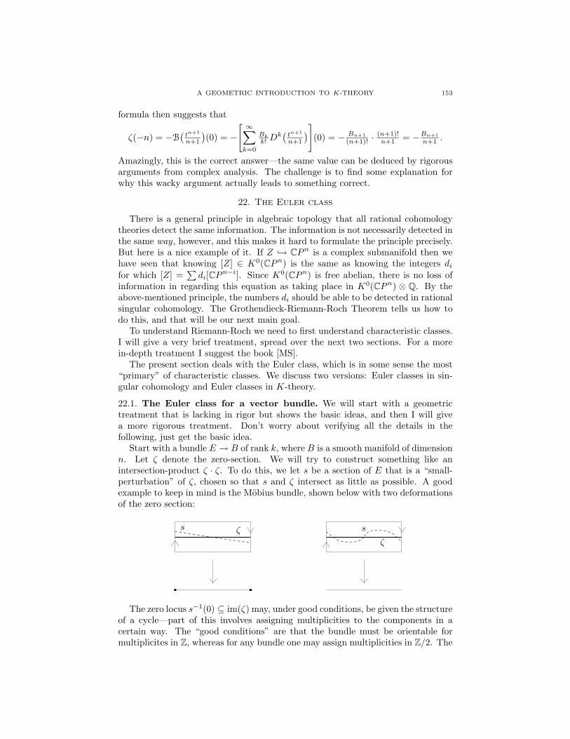
A GEOMETRIC INTRODUCTION TO K-THEORY 153
formula then suggests that
ζ(−n) = −B(tn+1
n+1
)(0) = −
[ ∞∑k=0
Bk
k! Dk(tn+1
n+1
)](0) = − Bn+1
(n+1)! ·(n+1)!n+1 = −Bn+1
n+1 .
Amazingly, this is the correct answer—the same value can be deduced by rigorousarguments from complex analysis. The challenge is to find some explanation forwhy this wacky argument actually leads to something correct.
22. The Euler class
There is a general principle in algebraic topology that all rational cohomologytheories detect the same information. The information is not necessarily detected inthe same way , however, and this makes it hard to formulate the principle precisely.But here is a nice example of it. If Z → CPn is a complex submanifold then wehave seen that knowing [Z] ∈ K0(CPn) is the same as knowing the integers difor which [Z] =
∑di[CPn−i]. Since K0(CPn) is free abelian, there is no loss of
information in regarding this equation as taking place in K0(CPn) ⊗ Q. By theabove-mentioned principle, the numbers di should be able to be detected in rationalsingular cohomology. The Grothendieck-Riemann-Roch Theorem tells us how todo this, and that will be our next main goal.
To understand Riemann-Roch we need to first understand characteristic classes.I will give a very brief treatment, spread over the next two sections. For a morein-depth treatment I suggest the book [MS].
The present section deals with the Euler class, which is in some sense the most“primary” of characteristic classes. We discuss two versions: Euler classes in sin-gular cohomology and Euler classes in K-theory.
22.1. The Euler class for a vector bundle. We will start with a geometrictreatment that is lacking in rigor but shows the basic ideas, and then I will givea more rigorous treatment. Don’t worry about verifying all the details in thefollowing, just get the basic idea.
Start with a bundle E → B of rank k, where B is a smooth manifold of dimensionn. Let ζ denote the zero-section. We will try to construct something like anintersection-product ζ · ζ. To do this, we let s be a section of E that is a “small-perturbation” of ζ, chosen so that s and ζ intersect as little as possible. A goodexample to keep in mind is the Mobius bundle, shown below with two deformationsof the zero section:
ζs
ζ
s
The zero locus s−1(0) ⊆ im(ζ) may, under good conditions, be given the structureof a cycle—part of this involves assigning multiplicities to the components in acertain way. The “good conditions” are that the bundle must be orientable formultiplicites in Z, whereas for any bundle one may assign multiplicities in Z/2. The

154 DANIEL DUGGER
dimension of this cycle is dim ζ + dim ζ − dimE, which is n+ n− (n+ k) = n− k.This cycle clearly depends on the choice of s, but a different choice of s givesa homologous cycle. So the associated class in homology is independent of ourchoices, and is an invariant of E. We call it the homology Euler class of E: fororientable bundles we have
eH(E) = ζ · ζ = s−1(0) ∈ Hn−k(B),
whereas for arbitrary bundles we have eH(E) ∈ Hn−k(B; Z/2). The sections s usedhere are usually referred to as “generic sections” of E.
The following are easy properties of the Euler class construction:(1) if E has a nonvanishing section, the eH(E) = 0, and(2) eH(E ⊕ F ) = eH(E) · eH(F ) (where · is the intersection product).(3) If L1 and L2 are line bundles on B then eH(L1 ⊗ L2) = eH(L1) + eH(L2).
For (1) we simply note that if σ is a nonvanishing section then the deformationt 7→ tσ (for t ∈ [0, 1]) allows us to regard s as a deformation of the zero-section.Taking s = εσ for small ε, the vanishing locus of s is the same as the vanishinglocus of σ—which is the empytset. So eH(E) = 0.
For (2), if s is a generic section of E and s′ is a generic section of F then s⊕ s′is a generic section of E⊕F . The vanishing locus of s⊕ s′ is the intersection of thevanishing loci of s and s′.
For (3), if s1 and s2 are generic sections of L1 and L2 then s1 ⊗ s2 is a genericsection of L1⊗L2. But s1⊗s2 vanishes at points in B where either s1 or s2 vanish.So the vanishing locus of s1 ⊗ s2 is the union of the vanishing loci of s1 and s2.
Example 22.2.(a) For the Mobius bundle M → S1 we have eH(M) = [∗] ∈ H0(S1; Z/2), as is
clearly depicted in the pictures above. Note the necessity of Z/2-coefficientshere.
(b) If B is an orientable, smooth manifold of dimension d, then eH(TB) ∈ H0(B).So eH(TB) is a multiple of [∗], and this multiple is precisely the Euler char-acteristic χ(B): a section of TB is just a vector field on B, and so this is theclassical statement that a generic vector field on B vanishes at precisely χ(B)points. This connection with the Euler characteristic is why eH is called theEuler class.
(c) Let L→ RPn be the tautological line bundle, and recall that L ∼= L∗. We exam-ine L∗ instead, since it is easier to write down formulas for sections. Genericallychoose a tuple α = (α1, . . . , αn) ∈ Rn and consider the section sα whose valueover x = [x0 : · · · : xn] is the functional sending (x0, . . . , xn) to α0x0+· · ·+αnxn.The vanishing locus for this section is a linear subspace of RPn, and of coursewe know that all such things are homotopic. So eH(γ) = [RPn−1].
(d) A similar analysis allows one to calculare eH(L∗) where L → CPn is the tau-tological line bundle, but here one must be careful about getting the signscorrect. It is clear enough that eH(L∗) = ±[CPn−1], but determining the signtakes some thought. ?????
(e) Normal bundle of Z → CPn????
22.3. Cohomology version. Let E → B be an orientable real bundle of rank k;that is, a bundle with a Thom class UE ∈ Hk(E,E − 0). Note that B need nolonger be a manifold. Let ζ : B → E denote the zero section, as usual. We may
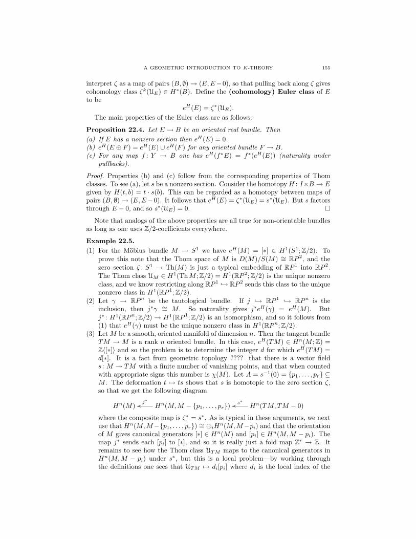
A GEOMETRIC INTRODUCTION TO K-THEORY 155
interpret ζ as a map of pairs (B, ∅)→ (E,E−0), so that pulling back along ζ givescohomology class ζk(UE) ∈ H∗(B). Define the (cohomology) Euler class of Eto be
eH(E) = ζ∗(UE).The main properties of the Euler class are as follows:
Proposition 22.4. Let E → B be an oriented real bundle. Then(a) If E has a nonzero section then eH(E) = 0.(b) eH(E ⊕ F ) = eH(E) ∪ eH(F ) for any oriented bundle F → B.(c) For any map f : Y → B one has eH(f∗E) = f∗(eH(E)) (naturality under
pullbacks).
Proof. Properties (b) and (c) follow from the corresponding properties of Thomclasses. To see (a), let s be a nonzero section. Consider the homotopyH : I×B → Egiven by H(t, b) = t · s(b). This can be regarded as a homotopy between maps ofpairs (B, ∅)→ (E,E−0). It follows that eH(E) = ζ∗(UE) = s∗(UE). But s factorsthrough E − 0, and so s∗(UE) = 0.
Note that analogs of the above properties are all true for non-orientable bundlesas long as one uses Z/2-coefficients everywhere.
Example 22.5.(1) For the Mobius bundle M → S1 we have eH(M) = [∗] ∈ H1(S1; Z/2). To
prove this note that the Thom space of M is D(M)/S(M) ∼= RP 2, and thezero section ζ : S1 → Th(M) is just a typical embedding of RP 1 into RP 2.The Thom class UM ∈ H1(ThM ; Z/2) = H1(RP 2; Z/2) is the unique nonzeroclass, and we know restricting along RP 1 → RP 2 sends this class to the uniquenonzero class in H1(RP 1; Z/2).
(2) Let γ → RPn be the tautological bundle. If j → RP 1 → RPn is theinclusion, then j∗γ ∼= M . So naturality gives j∗eH(γ) = eH(M). Butj∗ : H1(RPn; Z/2) → H1(RP 1; Z/2) is an isomorphism, and so it follows from(1) that eH(γ) must be the unique nonzero class in H1(RPn; Z/2).
(3) LetM be a smooth, oriented manifold of dimension n. Then the tangent bundleTM → M is a rank n oriented bundle. In this case, eH(TM) ∈ Hn(M ; Z) =Z〈[∗]〉 and so the problem is to determine the integer d for which eH(TM) =d[∗]. It is a fact from geometric topology ???? that there is a vector fields : M → TM with a finite number of vanishing points, and that when countedwith appropriate signs this number is χ(M). Let A = s−1(0) = p1, . . . , pr ⊆M . The deformation t 7→ ts shows that s is homotopic to the zero section ζ,so that we get the following diagram
Hn(M) Hn(M,M − p1, . . . , pr)j∗oo Hn(TM,TM − 0)s∗oo
where the composite map is ζ∗ = s∗. As is typical in these arguments, we nextuse that Hn(M,M−p1, . . . , pr) ∼= ⊕iHn(M,M−pi) and that the orientationof M gives canonical generators [∗] ∈ Hn(M) and [pi] ∈ Hn(M,M − pi). Themap j∗ sends each [pi] to [∗], and so it is really just a fold map Zr → Z. Itremains to see how the Thom class UTM maps to the canonical generators inHn(M,M − pi) under s∗, but this is a local problem—by working throughthe definitions one sees that UTM 7→ di[pi] where di is the local index of the
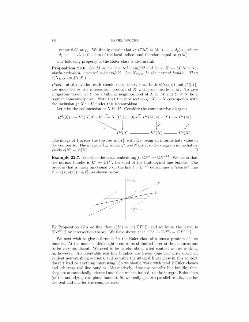
156 DANIEL DUGGER
vector field at pi. We finally obtain that eH(TM) = (d1 + · · · + dr)[∗], whered1 + · · ·+ dr is the sum of the local indices and therefore equal to χ(M).
The following property of the Euler class is also useful:
Proposition 22.6. Let M be an oriented manifold and let j : X → M be a reg-ularly embedded, oriented submanifold. Let NM/X be the normal bundle. Thene(NM/X) = j∗([X]).
Proof. Intuitively the result should make sense, since both e(NM/X) and j∗([X])are modelled by the intersection product of X with itself inside of M . To givea rigorous proof, let U be a tubular neighborhood of X in M and U ∼= N be aregular homeomorphism. Note that the zero section ζ : X → N corresponds withthe inclusion j : X → U under this isomorphism.
Let c be the codimension of X in M . Consider the commutative diagram
H0(X) // Hc(N,N − 0)
ζ∗ ''OOOOOOOOOOO
∼= // Hc(U,U − 0)
Hc(M,M −X)∼=oo
j∗
// Hc(M)
j∗
Hc(X) Hc(X) Hc(X).
The image of 1 across the top row is [X], with UN being an intermediate value inthe composite. The image of UN under ζ∗ is e(N), and so the diagram immediatelyyields e(N) = j∗[X].
Example 22.7. Consider the usual embedding j : CPn → CPn+1. We claim thatthe normal bundle is L∗ → CPn, the dual of the tautological line bundle. Theproof is that a linear functional φ on the line ` ⊆ Cn+1 determines a “nearby” line`′ = (x, φ(x))x ∈ `, as shown below:
en+2
Cn+1
`
`′
By Proposition 22.6 we find that e(L∗) = j∗([CPn]), and we know the latter is[CPn−1] by intersection theory. We have shown that e(L∗ → CPn) = [CPn−1].
We next wish to give a formula for the Euler class of a tensor product of linebundles. At the moment this might seem to be of limited interest, but it turns outto be very significant. We need to be careful about what context we are workingin, however. All orientable real line bundles are trivial (one can write down anevident nonvanishing section), and so using the integral Euler class in this contextdoesn’t lead to anything interesting. So we should work with mod 2 Euler classesand arbitrary real line bundles. Alternatively, if we use complex line bundles thenthey are automatically oriented and then we can indeed use the integral Euler class(of the underlying real plane bundle). So we really get two parallel results, one forthe real and one for the complex case:
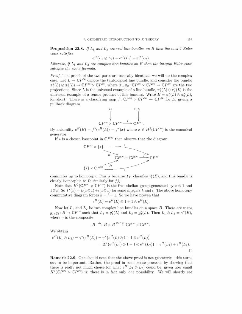
A GEOMETRIC INTRODUCTION TO K-THEORY 157
Proposition 22.8. If L1 and L2 are real line bundles on B then the mod 2 Eulerclass satisfies
eH(L1 ⊗ L2) = eH(L1) + eH(L2).Likewise, if L1 and L2 are complex line bundles on B then the integral Euler classsatisfies the same formula.
Proof. The proofs of the two parts are basically identical; we will do the complexcase. Let L → CP∞ denote the tautological line bundle, and consider the bundleπ∗1(L) ⊗ π∗2(L) → CP∞ × CP∞, where π1, π2 : CP∞ × CP∞ → CP∞ are the twoprojections. Since L is the universal example of a line bundle, π∗1(L)⊗π∗2(L) is theuniversal example of a tensor product of line bundles. Write E = π∗1(L) ⊗ π∗2(L),for short. There is a classifying map f : CP∞ × CP∞ → CP∞ for E, giving apullback diagram
E //
L
CP∞ × CP∞
f // CP∞.By naturality eH(E) = f∗(eH(L)) = f∗(x) where x ∈ H2(CP∞) is the canonicalgenerator.
If ∗ is a chosen basepoint in CP∞ then observe that the diagram
CP∞ × ∗
j2 **UUUUUUUUid
''CP∞ × CP∞
f // CP∞
∗ × CP∞j1
44iiiiiiii
id
77
commutes up to homotopy. This is because fj1 classifies j∗1 (E), and this bundle isclearly isomorphic to L; similarly for fj2.
Note that H2(CP∞ × CP∞) is the free abelian group generated by x ⊗ 1 and1⊗x. So f∗(x) = k(x⊗1)+ l(1⊗x) for some integers k and l. The above homotopycommutative diagram forces k = l = 1. So we have proven that
eH(E) = eH(L)⊗ 1 + 1⊗ eH(L).
Now let L1 and L2 be two complex line bundles on a space B. There are mapsg1, g2 : B → CP∞ such that L1 = g∗1(L) and L2 = g∗2(L). Then L1 ⊗ L2 = γ∗(E),where γ is the composite
B∆−→ B ×B g1×g2−→ CP∞ × CP∞.
We obtain
eH(L1 ⊗ L2) = γ∗(eH(E)) = γ∗(eH(L)⊗ 1 + 1⊗ eH(L)
)= ∆∗(eH(L1)⊗ 1 + 1⊗ eH(L2)
)= eH(L1) + eH(L2).
Remark 22.9. One should note that the above proof is not geometric—this turnsout to be important. Rather, the proof in some sense proceeds by showing thatthere is really not much choice for what eH(L1 ⊗ L2) could be, given how smallH∗(CP∞ × CP∞) is; there is in fact only one possibility. We will shortly see
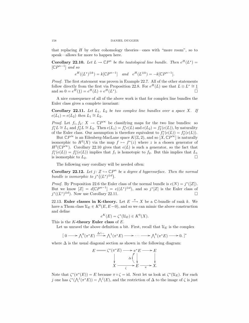
158 DANIEL DUGGER
that replacing H by other cohomology theories—ones with “more room”, so tospeak—allows for more to happen here.
Corollary 22.10. Let L → CPn be the tautological line bundle. Then eH(L∗) =[CPn−1] and so
eH((L∗)⊗k) = k[CPn−1] and eH(L⊗k) = −k[CPn−1].
Proof. The first statement was proven in Example 22.7. All of the other statementsfollow directly from the first via Proposition 22.8. For eH(L) use that L⊗ L∗ ∼= 1and so 0 = eH(1) = eH(L) + eH(L∗).
A nice consequence of all of the above work is that for complex line bundles theEuler class gives a complete invariant:
Corollary 22.11. Let L1, L2 be two complex line bundles over a space X. Ife(L1) = e(L2) then L1
∼= L2.
Proof. Let f1, f2 : X → CP∞ be classifying maps for the two line bundles: sof∗1L
∼= L1 and f∗2L ∼= L2. Then e(L1) = f∗1 e(L) and e(L2) = f∗2 (e(L)), by naturalityof the Euler class. Our assumption is therefore equivalent to f∗1 (e(L)) = f∗2 (e(L)).
But CP∞ is an Eilenberg-MacLane space K(Z, 2), and so [X,CP∞] is naturallyisomorphic to H2(X) via the map f 7→ f∗(z) where z is a chosen generator ofH2(CP∞). Corollary 22.10 gives that e(L) is such a generator, so the fact thatf∗1 (e(L)) = f∗2 (e(L)) implies that f1 is homotopic to f2. But this implies that L1
is isomorphic to L2.
The following easy corollary will be needed often:
Corollary 22.12. Let j : Z → CPn be a degree d hypersurface. Then the normalbundle is isomorphic to j∗
((L∗)⊗d
).
Proof. By Proposition 22.6 the Euler class of the normal bundle is e(N) = j∗([Z]).But we know [Z] = d[CPn−1] = e((L∗)⊗d), and so j∗[Z] is the Euler class ofj∗((L∗)⊗d). Now use Corollary 22.11.
22.13. Euler classes in K-theory. Let E π−→ X be a C-bundle of rank k. Wehave a Thom class UE ∈ K0(E,E−0), and so we can mimic the above constructionand define
eK(E) = ζ∗(UE) ∈ K0(X).This is the K-theory Euler class of E.
Let us unravel the above definition a bit. First, recall that UE is the complex
[ 0 // /\0(π∗E)∆∧− // /\1(π∗E) // . . . // /\k(π∗E) // 0. ]∗
where ∆ is the usual diagonal section as shown in the following diagram:
E ζ∗(π∗E) //
π∗E //
E
X
ζ// E π
//
∆
BB
X.
Note that ζ∗(π∗(E)) = E because π ζ = id. Next let us look at ζ∗(UE). For eachj one has ζ∗(/\j(π∗E)) = /\j(E), and the restriction of ∆ to the image of ζ is just
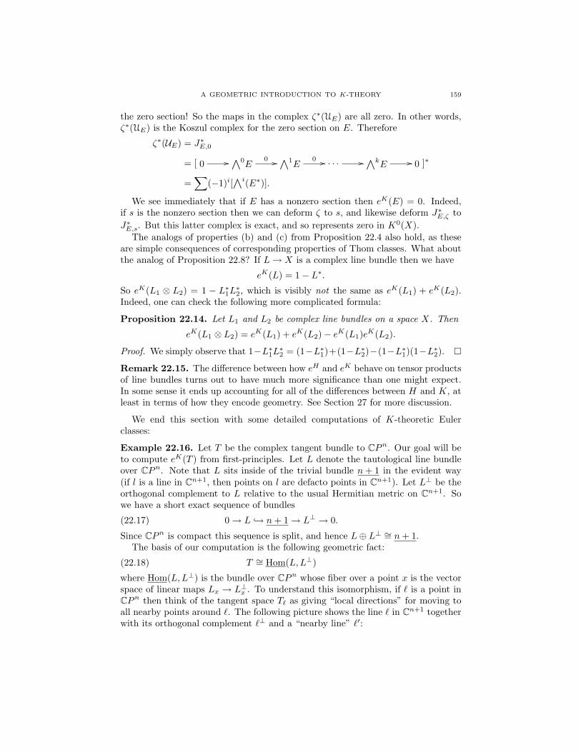
A GEOMETRIC INTRODUCTION TO K-THEORY 159
the zero section! So the maps in the complex ζ∗(UE) are all zero. In other words,ζ∗(UE) is the Koszul complex for the zero section on E. Therefore
ζ∗(UE) = J∗E,0
= [ 0 // /\0E
0 // /\1E
0 // . . . // /\kE // 0 ]∗
=∑
(−1)i[/\i(E∗)].
We see immediately that if E has a nonzero section then eK(E) = 0. Indeed,if s is the nonzero section then we can deform ζ to s, and likewise deform J∗E,ζ toJ∗E,s. But this latter complex is exact, and so represents zero in K0(X).
The analogs of properties (b) and (c) from Proposition 22.4 also hold, as theseare simple consequences of corresponding properties of Thom classes. What aboutthe analog of Proposition 22.8? If L→ X is a complex line bundle then we have
eK(L) = 1− L∗.So eK(L1 ⊗ L2) = 1 − L∗1L∗2, which is visibly not the same as eK(L1) + eK(L2).Indeed, one can check the following more complicated formula:
Proposition 22.14. Let L1 and L2 be complex line bundles on a space X. Then
eK(L1 ⊗ L2) = eK(L1) + eK(L2)− eK(L1)eK(L2).
Proof. We simply observe that 1−L∗1L∗2 = (1−L∗1)+(1−L∗2)−(1−L∗1)(1−L∗2).
Remark 22.15. The difference between how eH and eK behave on tensor productsof line bundles turns out to have much more significance than one might expect.In some sense it ends up accounting for all of the differences between H and K, atleast in terms of how they encode geometry. See Section 27 for more discussion.
We end this section with some detailed computations of K-theoretic Eulerclasses:
Example 22.16. Let T be the complex tangent bundle to CPn. Our goal will beto compute eK(T ) from first-principles. Let L denote the tautological line bundleover CPn. Note that L sits inside of the trivial bundle n+ 1 in the evident way(if l is a line in Cn+1, then points on l are defacto points in Cn+1). Let L⊥ be theorthogonal complement to L relative to the usual Hermitian metric on Cn+1. Sowe have a short exact sequence of bundles
0→ L → n+ 1→ L⊥ → 0.(22.17)
Since CPn is compact this sequence is split, and hence L⊕ L⊥ ∼= n+ 1.The basis of our computation is the following geometric fact:
T ∼= Hom(L,L⊥)(22.18)
where Hom(L,L⊥) is the bundle over CPn whose fiber over a point x is the vectorspace of linear maps Lx → L⊥x . To understand this isomorphism, if ` is a point inCPn then think of the tangent space T` as giving “local directions” for moving toall nearby points around `. The following picture shows the line ` in Cn+1 togetherwith its orthogonal complement `⊥ and a “nearby line” `′:
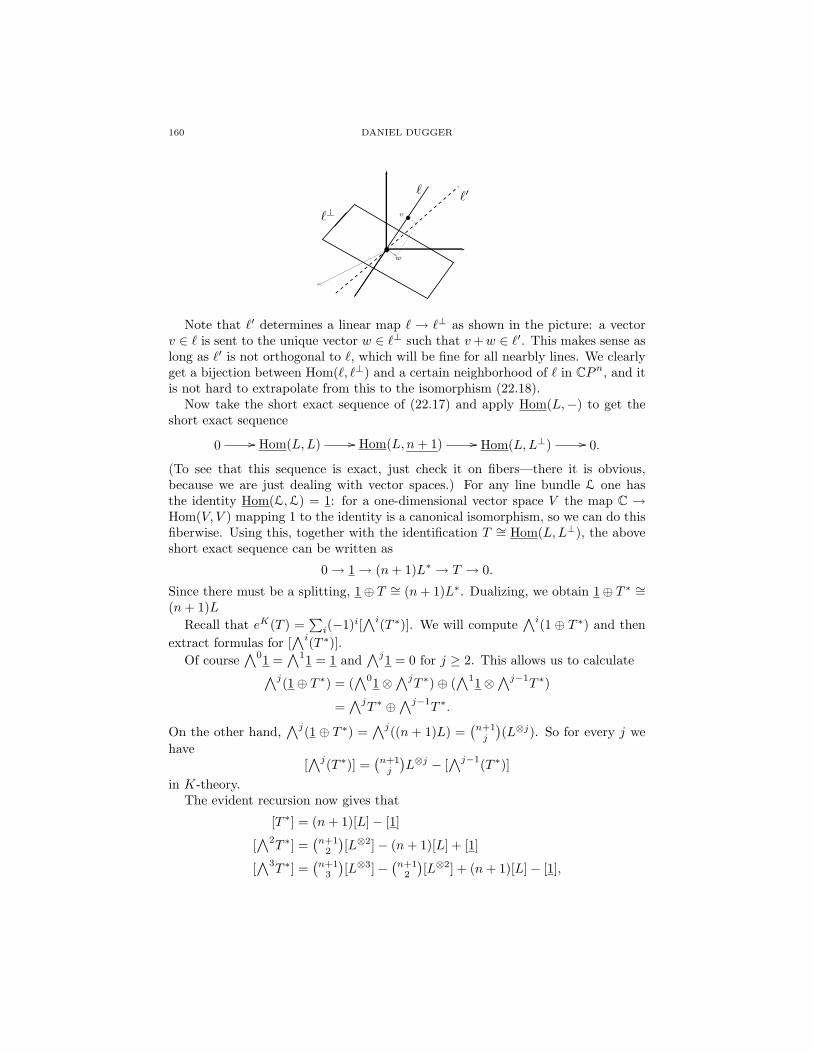
160 DANIEL DUGGER
`
`⊥`′
v
w
Note that `′ determines a linear map ` → `⊥ as shown in the picture: a vectorv ∈ ` is sent to the unique vector w ∈ `⊥ such that v+w ∈ `′. This makes sense aslong as `′ is not orthogonal to `, which will be fine for all nearbly lines. We clearlyget a bijection between Hom(`, `⊥) and a certain neighborhood of ` in CPn, and itis not hard to extrapolate from this to the isomorphism (22.18).
Now take the short exact sequence of (22.17) and apply Hom(L,−) to get theshort exact sequence
0 // Hom(L,L) // Hom(L, n+ 1) // Hom(L,L⊥) // 0.
(To see that this sequence is exact, just check it on fibers—there it is obvious,because we are just dealing with vector spaces.) For any line bundle L one hasthe identity Hom(L,L) = 1: for a one-dimensional vector space V the map C →Hom(V, V ) mapping 1 to the identity is a canonical isomorphism, so we can do thisfiberwise. Using this, together with the identification T ∼= Hom(L,L⊥), the aboveshort exact sequence can be written as
0→ 1→ (n+ 1)L∗ → T → 0.
Since there must be a splitting, 1⊕ T ∼= (n+ 1)L∗. Dualizing, we obtain 1⊕ T ∗ ∼=(n+ 1)L
Recall that eK(T ) =∑i(−1)i[/\i(T ∗)]. We will compute /\i(1 ⊕ T ∗) and then
extract formulas for [/\i(T ∗)].Of course /\01 = /\11 = 1 and /\j1 = 0 for j ≥ 2. This allows us to calculate
/\j(1⊕ T ∗) = (/\01⊗ /\jT ∗)⊕ (/\11⊗ /\j−1T ∗)
= /\jT ∗ ⊕ /\j−1T ∗.
On the other hand, /\j(1 ⊕ T ∗) = /\j((n + 1)L) =(n+1j
)(L⊗j). So for every j we
have[/\j(T ∗)] =
(n+1j
)L⊗j − [/\j−1(T ∗)]
in K-theory.The evident recursion now gives that
[T ∗] = (n+ 1)[L]− [1]
[/\2T ∗] =
(n+1
2
)[L⊗2]− (n+ 1)[L] + [1]
[/\3T ∗] =
(n+1
3
)[L⊗3]−
(n+1
2
)[L⊗2] + (n+ 1)[L]− [1],
A GEOMETRIC INTRODUCTION TO K-THEORY 161
and so on. The general formula, obtained by an easy induction, is
[/\jT ∗] =j∑
k=0
(−1)k+j(n+1k
)[L⊗k].
This now lets us calculate
eK(T ) = (−1)n[(n+1
1
)[L]n − 2
(n+1
2
)[L]n−1 + 3
(n+1
3
)[L]n−2 − . . .
]= (−1)n(n+ 1)
[[L]n −
(n1
)[L]n−1 +
(n2
)[L]n−2 − . . .
]= (n+ 1)(1− [L])n.
Recall that (1− [L])n = [∗], and so we have determined that
eK(T ) = (n+ 1)[∗].Let us now confess that the result of this computation is not unexpected. Indeed,
we saw previously that eH(TM) = χ(M)[∗] for any smooth manifold M , and infact the same is true in any complex-oriented cohomology theory (by essentiallythe same proof). The “n + 1” in our formula for eK(T ) is just χ(CPn). Butnote that we computed this without writing down anything remotely resemblinga cell structure! In fact, the only geometry in the calculation was in the factT ∼= Hom(L,L⊥); everything else was some simple linear algebra and then basicalgebraic manipulation. It is useful to remember the overall theme of K-theory: dolinear algebra fiberwise over a base space X, and see what this tells you about thetopology of X. Our computation of eK(TCPn) gives an example of this.
The calculation in the above example is a little clunky. One way to streamlineit is to introduce the formal power series
λt(E) =∞∑i=0
ti[/\i(E)] = 1 + t[E] + t2[/\2(E)] + · · ·
which we regard as living in the ring K(X)[[t]], where E → X was a vector bundle.Notice that this is actually a polynomial in t, since the exterior powers vanishbeyond the rank of E; we consider it as a power series because in that context ithas a multiplicative inverse, which we will shortly need.
If L is a line bundle then λt(L) = 1 + t[L]. Also, the formula /\k(E ⊕ F ) =⊕i+j=k /\i(E)⊗ /\j(F ) yields the nice relation
λt(E ⊕ F ) = λt(E) · λt(F ).
This is what ultimately simplifies our calculations. Finally, notice that the K-theoretic Euler characteristic can be written as eK(E) = λt(E∗)|t=−1.
Returning to the above calculation, the starting point for the algebra was thebundle isomorphism 1⊕ T ∗ ∼= (n+ 1)L. Applying λt we obtain
λt(1)λt(T ∗) = λt(1⊕ T ∗) = λt((n+ 1)L∗) = (λt(L))n+1.
But λt(1) = 1 + t and λt(L) = 1 + t[L], so we can write
λt(T ∗) = (1+t[L])n+1
1+t , or eK(T ) = (1+t[L])n+1
1+t
∣∣∣t=−1
(and here is where we are using that our power series have multiplicative inverses).Our task is to expand the formula for eK(T ) into powers of t, and then to sett = −1. The trick is to do this in a clever way.
162 DANIEL DUGGER
We are going to ultimately want to write eK(T ) in terms of powers of (1 − L),as they give our usual basis for K∗(CPn). The trick is to do this before pluggingin t = −1, rather than afterwards. Regard L as a formal variable and considerf(L) = (1 + tL)n+1/(1 + t), regarded as a formal power series in two variables (butwhere we are choosing not to write t in the inputs of f). Let us expand this inpowers of (L− 1) via the usual Taylor series:
f(L) = f(1) + f ′(1)(L− 1) + f ′′(1)2 (L− 1)2 + · · ·
It is simple to compute that the coefficient of (L− 1)k is(n+1k
)(1 + t)n−k+1tk, and
so we obtain
λt(T ∗) =n+1∑k=0
(n+1k
)(1 + t)n−ktk(L− 1)k.
Notice that the substitution t = −1 will make the summands vanish for k smallerthan n, and that the term k = n+ 1 vanishes because (L− 1)n+1 = 0 in K(CPn).So we quickly find that
eK(T ) = λt(T ∗)|t=−1 =(n+1n
)tn(L− 1)n = (n+ 1)(1− L)n = (n+ 1)[∗].
Example 22.19 (Euler characteristic of a hypersurface). Using the λt operatorsintroduced above, we will attempt a harder computation of an Euler class. Letj : Z → CPn be a smooth hypersurface of degree d. Our goal is to compute theEuler characteristic χ(Z). If TZ and NZ denote the tangent and normal bundles,respectively, then TZ ⊕ NZ ∼= j∗TCPn . We know from Corollary 22.12 that NZ ∼=j∗O(d), so we have
1⊕ TZ ⊕ j∗O(d) ∼= 1⊕ j∗TCPn ∼= (n+ 1)j∗O(1).
Taking duals and applying λt, we obtain
λt(1) · λt(T ∗Z) · λt(j∗Ld) = λt(j∗L)n+1.
Let X = j∗L. Then we can write
λt(T ∗) = (1+tX)n+1
(1+t)(1+tXd).
We wish to compute the Euler class eK(T ) = λt(T ∗)|t=−1 and then write it in theform (???) · [∗], in which case the mystery number in parentheses will be χ(Z). Thetrick is again to expand in powers of (X − 1), since the powers of 1 − L are ourstandard generators for K0(CPn).
Consider the power series
f(X) = (1+tX)n+1
(1+t)(1+tXd)= f(t, 1) + f ′(1)(X − 1) + f ′′(1)
2 (X − 1)2 + · · ·
Note that (1−L)n+1 is zero inK0(CPn) and therefore (1−X)n+1 vanishes inK0(Z).Even better, (1−L)n = [∗] in K0(CPn) and since j∗[∗] = 0 by intersection theory itfollows that (1−X)n = 0 in K0(X). So we don’t care about any terms in the aboveseries beyond (X − 1)n−1. Let us also note at this point that (1 − L)n−1 = [CP 1]in K0(CPn), and therefore (1 −X)n−1 = j∗
((1 − L)n−1
)= j∗([CP 1]) = d[∗]; the
last equality holds by intersection theory, since a generic CP 1 will intersect Z inexactly d points.
A GEOMETRIC INTRODUCTION TO K-THEORY 163
Before tackling the general calculation let us do the first example, where n = 2.Here f(X) = (1+tX)3
(1+t)(1+tXd)and we only need the first two terms of the series. Clearly
f(1) = 1 + t and an easy calculation gives
f ′(X) = 11+t ·
(1+tX)2
(1+tXd)2
[3t(1 + tXd)− (1 + tX)tdXd−1]
so thatf ′(1) = (3− d)t.
Putting everything together,
f(X) = (1 + t) + (3− d)t(X − 1)
and so
eK(TZ) = f(X)|t=−1 = 0 + (d− 3)(X − 1) = (3− d)(1−X) = (d− 3) · d[∗].We conclude that χ(Z) = d(3− d).
For larger n here is how things are going to work. First, we will calculate thederivatives f (k)(1) for 0 ≤ k ≤ n− 1, and then substitute t = −1 into all of them.It will turn out (but is far from obvious) that the resulting expressions vanish fork < n− 1, so that
eK(TZ) = f (n−1)(1)|t=−1 · (X − 1)n−1
= f (n−1)(1)|t=−1 · (−1)n−1 · (1−X)n−1
= f (n−1)(1)|t=−1 · (−1)n−1 · d[∗].The conclusion will then be that
χ(Z) = f (n−1)(1)|t=−1 · (−1)n−1 · d.Notice that everything comes down to computing the expressions f (k)(1)|t=−1,
which is a purely algebraic problem. Unfortunately we cannot first plug in t = −1,since our formula for f has a 1 + t in the denominator; we have to first do the hardwork of writing f as a polynomial in t before plugging in. At first glance this worklooks very hairy! Already the formula for f ′(X) was quite complicated, and it onlygets worse for the higher derivatives. The reader might wish to carry this out bybrute force for n = 3, to get a feel for the difficulties.
We are going to sketch the completion of the calculations for the above exam-ple, but before diving into that we need to make a confession. It is possible tocompute χ(Z) by doing a similar kind of calculation using singular cohomologyinstead of K-theory, and in that setting the algebra turns out to be much easier !There is a trade-off, which is that the computation cannot be done merely withEuler classes—one needs the complete theory of Chern classes, to be developed inthe next section. See Example 23.7 for the computation of χ(Z) in that context.This situation is fairly typical of the relationship between K-theory and singularcohomology. For calculations that can be done in either theory, usually the singularcohomology version will involve simpler algebra, but more advanced geometric tech-niques; the K-theory version will involve more advanced algebra, but one needs lessgeometry. In some sense we saw this phenomenon already in the case of intersectionmultiplicities.
The completion of our calculation will proceed via the following steps:

164 DANIEL DUGGER
(a) Suppose that f(w) ∈ Q[w] has degree k. Then there is an identity of formalpower series
f(0)− tf(1) + t2f(2)− · · · = u(t)(1+t)k+1
for a unique polynomial u(t). Moreover, the degree of u(t) is at most k andu(−1) is k! times the leading coefficient of f .
To justify the above claim, write Af =∑k≥0(−1)kf(k)tk. Note the formula
(1+t)Af = f(0)−tA∆f where ∆ is the finite difference operator from Section 21.Check the claim is true when deg f = 0, and then do an induction on the degree.(Extra credit: Find a formula for u(t) in terms of the numbers ∆kf(0)).
(b) By collecting terms notice that1
1+tXd = 1− tXd + t2X2d − · · ·
= 1− t((X − 1) + 1)d + t2((X − 1) + 1)2d − · · ·= 1
1+t + (X − 1)Γ1 + (X − 2)Γ2 + · · ·where
Γk = −t(dk
)+ t2
(2dk
)− t3
(3dk
)+ · · ·
It follows from (a) that Γk = uk(t)(1+t)k+2 where uk(t) is a polynomial such that
u(−1) = dk.(c) Set fr = (1+tX)r
(1+t)(1+tXd). Notice the recursion relation
fr+1 = (1 + tX)fr = (1 + t((X − 1) + 1))fr = (1 + t)fr + (X − 1)tfr.
So if we know the expansion of fr in terms of powers of X − 1, it is easy toget the expansion of fr+1. In the following table, row r shows the terms in theexpansion for fr (starting with f0):
r (X − 1)0 (X − 1)1 (X − 1)2 (X − 1)3 · · ·0 1
(1+t)2u1
(1+t)3u2
(1+t)3u3
(1+t)3 · · ·
1 11+t
u1+t(1+t)2
u2+tu1(1+t)3
u3+tu2(1+t)3 · · ·
2 1 u1+2t(1+t)
u2+2tu1+t2
(1+t)2u3+2tu2+t
2u1(1+t)3 · · ·
3 1 + t u1 + 3t u2+3tu1+3t2
1+tu3+3tu2+2t2u1+t
3
(1+t)2 · · ·
4 (1 + t)2 (1+t)(u1+3t)+t(1+t) u2 + 4tu1 + 6t2 · · · · · ·
(c) Ignoring the terrible-looking formulas, one important thing is evident from thetable: in the column for (X − 1)r, after row r + 2 we are getting polynomialmultiples of 1+ t. So these entries will all vanish when we specialize to t = −1,and we see that in fr|t=−1 the first nonzero coefficient appears in the (X−1)r−2
term. Our job is to calculate this coefficient. In order to do so, notice that itsuffices to just look at all the numerators in the table; the denominators canbasically be ignored. To this end, let gr(W ) be the generating function forthe numerators in row r of the table, specialized to t = −1. For example,g0(W ) = 1 + dW + d2W 3 + · · · . The recursion relation for these numerators is
gr+1 = gr −Wgr = (1−W )gr.
A GEOMETRIC INTRODUCTION TO K-THEORY 165
So of course we will have
gr = (1−W )rg0 = (1−W )r · 11−dW = (1−W )r · (1 + dW + d2W 2 + · · · ).
The number we are looking for is the coefficient of W r−2 in this power series,and it is a simple matter to compute it. The desired coeffient is
dr−2 − dr−3(r1
)+ dr−4
(r2
)− · · ·+ (−1)r−2
(rr−2
).
(d) Now putting everything together, we have proven that
χ(Zd → CPn) = (−1)n+1d[dn−1 − dn−2
(n+1
1
)+ · · ·+ (−1)n−1
(n+1n−1
)]= (−1)n+1d ·
[(d−1)n+1−(−1)n+1((n+1)d−1)
d2
]= (1−d)n+1−((n+1)d−1)
d .
None of the above formulas are particularly pleasant to look at, and they aredifficult to remember. I like to encode the formula in a different way. Let `denote the formal “lowering operator” that sends ds to ds−1, for each s. Thenwe may write
χ(Zd → CPn) = d · (`− I)n+1(dn−1)where I is the identity operator. For example,
χ(Zd → CP 3) = d · (`4 − 4`3 + 6`2 − 4`+ I)(d2) = d · (6− 4d2 + d3).
23. Chern classes
Fix a certain collection of vector bundles. A characteristic class for this collec-tion assigns to each vector bundle E → X a cohomology class b(E) belonging tosome cohomology theory; the assignment is required to be natural. We have seenessentially two examples so far: for the collection of oriented, rank k vector bundles,we have the Euler classes eH and eK .
The Chern classes are characteristic classes for complex vector bundles, thatgeneralize the Euler class in a certain way. Like the Euler class, they have close tiesto geometry. Also like the Euler class, there are versions of Chern classes in bothsingular cohomology and K-theory—indeed, there are versions in any complex-oriented cohomology theory.
In this section we begin with a purely geometric look at the Chern classes, wherewe again forego all attempts at rigor. Afterwards we will pursue a more rigorousapproach, which can even be done axiomatically.
23.1. Geometric Chern classes in homology. Let B be a complex manifoldof dimension n, and let E → B be a complex vector bundle of rank k. If s is ageneric section of E, then the locus where s vanishes gives a cycle in B that carriesthe Euler class eH(E) ∈ H2(n−k)(B). This homology class will now be renamed asCk(E) and called the kth homology Chern class of E.
Now let s1 and s2 be two generic sections, chosen so that s1(x) and s2(x) arelinearly independent on as large a subset of B as possible. We can now look at thedegeneracy locus
D(s1, s2) = b ∈ B | s1(b) and s2(b) are linearly dependent.
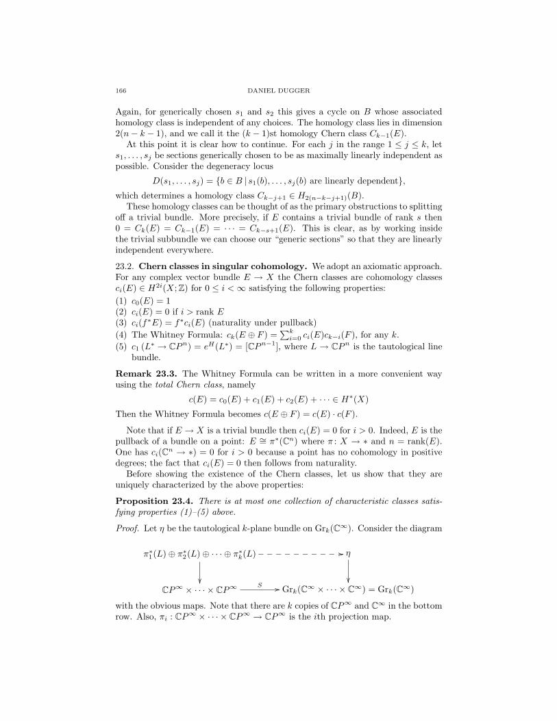
166 DANIEL DUGGER
Again, for generically chosen s1 and s2 this gives a cycle on B whose associatedhomology class is independent of any choices. The homology class lies in dimension2(n− k − 1), and we call it the (k − 1)st homology Chern class Ck−1(E).
At this point it is clear how to continue. For each j in the range 1 ≤ j ≤ k, lets1, . . . , sj be sections generically chosen to be as maximally linearly independent aspossible. Consider the degeneracy locus
D(s1, . . . , sj) = b ∈ B | s1(b), . . . , sj(b) are linearly dependent,which determines a homology class Ck−j+1 ∈ H2(n−k−j+1)(B).
These homology classes can be thought of as the primary obstructions to splittingoff a trivial bundle. More precisely, if E contains a trivial bundle of rank s then0 = Ck(E) = Ck−1(E) = · · · = Ck−s+1(E). This is clear, as by working insidethe trivial subbundle we can choose our “generic sections” so that they are linearlyindependent everywhere.
23.2. Chern classes in singular cohomology. We adopt an axiomatic approach.For any complex vector bundle E → X the Chern classes are cohomology classesci(E) ∈ H2i(X; Z) for 0 ≤ i <∞ satisfying the following properties:(1) c0(E) = 1(2) ci(E) = 0 if i > rank E(3) ci(f∗E) = f∗ci(E) (naturality under pullback)(4) The Whitney Formula: ck(E ⊕ F ) =
∑ki=0 ci(E)ck−i(F ), for any k.
(5) c1 (L∗ → CPn) = eH(L∗) = [CPn−1], where L → CPn is the tautological linebundle.
Remark 23.3. The Whitney Formula can be written in a more convenient wayusing the total Chern class, namely
c(E) = c0(E) + c1(E) + c2(E) + · · · ∈ H∗(X)
Then the Whitney Formula becomes c(E ⊕ F ) = c(E) · c(F ).
Note that if E → X is a trivial bundle then ci(E) = 0 for i > 0. Indeed, E is thepullback of a bundle on a point: E ∼= π∗(Cn) where π : X → ∗ and n = rank(E).One has ci(Cn → ∗) = 0 for i > 0 because a point has no cohomology in positivedegrees; the fact that ci(E) = 0 then follows from naturality.
Before showing the existence of the Chern classes, let us show that they areuniquely characterized by the above properties:
Proposition 23.4. There is at most one collection of characteristic classes satis-fying properties (1)–(5) above.
Proof. Let η be the tautological k-plane bundle on Grk(C∞). Consider the diagram
π∗1(L)⊕ π∗2(L)⊕ · · · ⊕ π∗k(L) //__________
η
CP∞ × · · · × CP∞ S // Grk(C∞ × · · · × C∞) = Grk(C∞)
with the obvious maps. Note that there are k copies of CP∞ and C∞ in the bottomrow. Also, πi : CP∞ × · · · × CP∞ → CP∞ is the ith projection map.
A GEOMETRIC INTRODUCTION TO K-THEORY 167
This diagram is a pullback diagram. Hence,
S∗(η) = (π∗1L)⊕ · · · ⊕ (π∗kL).
Applying cohomology to the map on the bottom row gives
H∗(CP∞ × · · · × CP∞) H∗(Grk(C∞))S∗oo .
By the Kunneth Theorem,
H∗(CP∞ × · · · × CP∞) ∼= H∗(CP∞)⊗ · · · ⊗H∗(CP∞) = Z[x1, . . . , xk]
where xi = π∗i (x) with x ∈ H2(CP∞) being the canonical generator. There isan evident action on CP∞ × · · · × CP∞ by the symmetric group Σk. This actiondescends in cohomology to give the statement
H∗(CP∞ × · · · × CP∞)Σk ∼=[H∗(CP∞)⊗ · · · ⊗H∗(CP∞)
]Σk
= Z[x1, . . . , xk]Σk
= Z[σ1, . . . , σk]
where σi is the ith elementary symmetric function in the xi’s.Recall that [X,Grk(C∞)] ' Vectk(X). Under this bijection, S corresponds to
the bundle E = ⊕iπ∗i (L). If α ∈ Σk then the map S α corresponds to thedirect sum of π∗i (L)’s but where the sum is taken in a different order. Since this isisomorphic to the original bundle E, is must be that S and S α are homotopic;in particular, they induced the same map on cohomology. Since this holds for allα, it follows that S∗ lands inside the Σk invariants. That is, S∗ can be regarded asa map
H∗(Grk(C∞)) S∗−→[H∗(CP∞)⊗k
]Σk
= Z[σ1, . . . , σk].
It is a theorem that the above map S∗ is an isomorphism. We will not take thetime to prove this, but the idea is simple enough. The Schubert cell decompositionof Grk(C∞) has all cells in even dimensions, and hence the coboundary maps areall zero; this computes H∗(Grk(C∞)) additively, and one readily checks that thegroups have the same ranks as in Z[σ1, . . . , σk]. ????
Using the Whitney Formula (iteratively), we can see that
ci(π∗1L⊕ · · · ⊕ π∗kL) =∑β
c1(π∗β(1)(L)) · c1(π∗β(2)(L)) . . . c1(π∗β(i)(L))
=∑β
π∗β(1)(x) · π∗β(2)(x) . . . π
∗β(i)(x)
where the sum ranges over strictly-increasing maps β : 1, . . . , i → 1, . . . , k, andin the second sum x = c1(L) ∈ H2(CP∞). But note that if we write xj = π∗j (x)then the second sum is simply the elementary symmetric function σi in the xj ’s.
It follows from the above that ci(η) is the unique element of H2i(Grk(C∞)) thatmaps to σi under S∗.
Finally, suppose that E → X is any complex vector bundle, say of rank k. Thenthere is a map f : X → Grk(C∞) and an isomorphism f∗η ∼= E. It follows thatci(E) = f∗(ci(η)).
To complete the proof, assume that c∗ and c′∗ are two sets of characteristic classessatisfying properties (1)–(5). Then ci(η) and c′i(η) must agree, for they each must
168 DANIEL DUGGER
be the unique element of H2i(Grk(C∞)) that maps to σi. It then follows fromnaturality that ci(E) = c′i(E) for all bundles E.
By examining the above proof, one finds that we can define the Chern classesin the following way. First, when η → Grk(C∞) is the tautological bundle thendefine ci(η) to be the unique element of H2i(Grk(C∞)) that maps to σi under S∗.Second, for an arbitrary bundle E → X let f : X → Grk(C∞) be a classifying mapand define ci(E) = f∗(ci(η)).
Remark 23.5. For a bundle E → X one can also define K-theoretic Chern classescKi (E) ∈ K0(X) (or really in K2i(X), but this is the same by periodicity). We willnot pursue this at the moment, but see ????
Example 23.6. Consider the tangent bundle T = TCPn → CPn. We saw inExample 22.16 that 1⊕ T ∼= (n+ 1)L∗. Then by the Whitney Formula,
c(T ) = c(1) · c(T ) = c(1⊕ T ) = c(L∗)n+1 = (1 + [CPn−1])n+1.
Therefore,ci(T ) =
(n+1i
)[CPn−i] =
(n+1i
)xi
where x ∈ H2(CPn) is the canonical generator [CPn−1]. Note that the Eulerclass is e(T ) = cn(T ) = (n + 1)xn = (n + 1)[∗], and so this again calculates thatχ(CPn) = n+ 1.
Example 23.7. Consider a hypersurface j : Z → CPn of degree d. Recall fromCorollary 22.12 that the normal bundle of this inclusion is j∗O(d), and we knowTZ ⊕NZ ∼= j∗TCPn . Then applying total Chern classes we get
c(TZ) · c(NZ) = j∗c(TCPn).
But above we calculated that c(TCPn) = (1 + x)n+1, and c(NZ) = c(j∗O(d)) =j∗(c(Od)) = 1 + d(j∗x). Let z = j∗x, so that we have
c(TZ) = (1+z)n+1
1+dz = (1 + (n+ 1)z +(n+1
2
)z2 + · · · ) · (1− dz + d2z2 − · · · ).
We can compute χ(Z) by finding the top Chern class (the Euler class), which inthis case is cn−1(TZ). A direct computation shows that
cn−1(TZ) = zn−1 ·((n+1n−1
)−(n+1n−2
)d+
(n+1n−2
)d2 − · · ·
).
Finally, we need to remember that xn−1 = [CP 1] in H∗(CPn) and therefore zn−1 =j∗(xn−1) = d[∗], since a generic line intersects Z in d distinct points. So we have
cn−1(TZ) = [∗] · d · ((n+1n−1
)−(n+1n−2
)d+
(n+1n−2
)d2 − · · ·
),
thereby yielding
χ(Z) = d ·((
n+1n−1
)−(n+1n−2
)d+
(n+1n−2
)d2 − · · ·
).
For example, a degree d hypersurface in CP 2 has χ(Z) = d · (3− d) and a degree dhypersurface in CP 3 has χ(Z) = d · (6− 4d+ d2).

A GEOMETRIC INTRODUCTION TO K-THEORY 169
23.8. Stiefel-Whitney classes. One can repeat almost all of our above work inthe setting of real vector bundles, but using Z/2 coefficients everywhere. Theanalogs of the Chern classes in this setting are called Stiefel-Whitney classes.If E → X is a real vector bundle then the Stiefel-Whitney classes are cohomol-ogy classes wi(E) ∈ Hi(X; Z/2), 0 ≤ i < ∞, satisfying the evident analogs of theaxioms in Section 23.2. Geometrically, these are Poincare Duals of certain cyclesdetermined by degeneracy loci, just as in the complex case. In terms of our develop-ment, most things go through verbatim but the one exception is the computationH∗(Grk(R∞); Z/2) ∼= Z/2[σ1, . . . , σk]. In the complex case this was fairly easy,because the standard cell structure on Grk(C∞) has cells only in even dimensions.This is of course not true for Grk(R∞), and so one must work a bit harder here.We will not give details; see [MS].
Just as for the Chern classes, we will write w(E) for the total Stiefel-Whitneyclass 1 + w1(E) + w2(E) + · · · .
Example 23.9. Here is an example where we can use Stiefel-Whitney classes tosolve a problem that appeared earlier in these notes. Let γ → RPn denote thetautological line bundle, and recall that once upon a time we needed to knowwhether γ ⊕ γ was stably trivial. This came up (for n = 2) in Section 13.10 duringthe course of trying to compute KO(RP 2).
If (γ ⊕ γ)⊕N ∼= N + 2 then applying total Stiefel-Whitney classes gives
1 = w(N + 2) = w(γ ⊕ γ ⊕N) = w(γ) · w(γ) · w(N) = w(γ)2.
But γ is a line bundle, so wi(γ) = 0 for i > 1 and w1(γ) is the mod 2 Euler class,which we have previously computed to be the generator x on H1(RPn; Z/2). Sow(γ) = 1 + x and therefore w(γ)2 = 1 + x2. As long as n ≥ 2 this is not equal to1, and hence γ ⊕ γ cannot be stably trivial.
Example 23.10. Let T be the tangent bundle of RPn. Just as in Example 22.16there is an isomorphism 1⊕T ∼= (n+1)L∗, where L→ RPn is the tautological linebundle. But since we are now in the case of real bundles, L ∼= L∗ by Corollary 8.23;so we will usually write 1⊕ T ∼= (n+ 1)L. One of course finds that
w(T ) = w(1⊕ T ) = w((n+ 1)L) = w(L)n+1 = (1 + x)n+1,
similarly to the complex case.
24. Comparing K-theory and singular cohomology
We have seen that singular cohomology and K-theory both encode geometryin similar ways: they have Thom classes, Euler classes, fundamental classes forsubmanifolds, etc. They can both be used to compute intersection multiplicities.One might hope for a natural transformation from one to the other, that allows oneto directly compare what is happening in each theory. Our goal in this section is toconstruct such a natural transformation, with some caveats which we will discoveralong the way.
Let us imagine that we have a natural transformation φ : K∗(−) → H∗(−),and that this is a ring homomorphism. Note first that φ cannot preserve thegradings, for β ∈ K−2(pt) is a unit whereas there is no unit in H−2(pt). We can fixthis by formally adjoining a unit to H∗: let H∗[t, t−1] be the cohomology theoryX 7→ H∗(X)[t, t−1], where t is given degree −2. Then we can ask for a natural

170 DANIEL DUGGER
ring homomorphism φ : K∗(−)→ H∗(−)[t, t−1]. Restricting to ∗ = 0 would give anatural ring homomorphism
φ : K0(−)→ Hev(−) = ⊕iH2i(−).
We will investigate what this map can look like.If L→ X is a complex line bundle then we have the element eK(L) ∈ K0(X), in
some sense representing the intersection of the zero-section with itself. One’s firstguess would be that φ should send eK(L) to eH(L), as the latter represents thesame ‘geometry’ inside of H∗. However, this hypothesis is not compatible with φbeing a ring homomorphism. Recall that
eK(L1 ⊗ L2) = eK(L1) + eK(L2)− eK(L1)eK(L2),
whereaseH(L1 ⊗ L2) = eH(L1) + eH(L2).
These formulas are incompatible.So it cannot be that φ sends eK(L) to eH(L). However, it is guaranteed that
eK(L) must be sent to some algebraic expression involving eH(L). Indeed, this isobviously so for the tautological bundle L → CP∞, since eH(L) is a generator ofH2(CP∞) and everything else in H∗(CP∞) is a polynomial in this generator; thecase for general line bundles then follows from naturality.
So we know that we will have φ send eK(L) 7→ f(eH(L)) where f(x) ∈ Z[[x]].Note that when X is compact then sufficiently large powers of eH(L) will be zero,so in practice f(eH(L)) is really just a polynomial in eH(L). Using a power seriesallows us to treat all spaces X at once, without assuming some uniform bound ontheir dimensions.
Let f(x) = α0 +α1x+α2x2 + . . . be the expansion for f . Note that if L→ X is
a trivial bundle then both eK(L) and eH(L) are zero, and from this it follows thatα0 = 0. Next note that if φ is a ring homomorphism then we must have
f(eH(L1) + eH(L2)) = f(eH(L1 ⊗ L2))
= φ(eK(L1 ⊗ L2))
= φ(eK(L1) + eK(L2)− eK(L1)eK(L2))
= f(eH(L1)) + f(eH(L2))− f(eH(L1))f(eH(L2)).
This suggests that we’re looking for f(x) ∈ Z[[x]] such that
f(a+ b) = f(a) + f(b)− f(a)f(b).(24.1)
We can take two approaches to determine the coefficients of such an f .
Approach 1. Substitute f(x) =∑i αix
i into (24.1) to get
LHS = α0 + α1(a+ b) + α2(a+ b)2 + . . .
and
RHS = [α0 + α1a+ α2a2 + . . . ] + [α0 + α1b+ α2b
2 + . . . ]
− [α0 + α1a+ α2a2 + . . . ][α0 + α1b+ α2b
2 + . . . ].
By expanding and equating coefficients, we can determine the coefficients αi. Thefirst equation is α2
0 = α0, and since α0 6= 0 this means α0 = 1. It turns outthere is no equation determining α1, but looking at the coefficient of abn−1 yields
A GEOMETRIC INTRODUCTION TO K-THEORY 171
nαn = −α1αn−1, or αn = −α1αn−1n . So by induction αn = (−1)n−1 α
n1n! . Note, in
particular, this last equation: it shows that f cannot have integral coefficients, aswe were orginally guessing! So we can only make things work if the target of φ isHev(−; Q).
We have been led to the conclusion f(x) = 1−e−α1x, and the reader may readilycheck that this does indeed yield a power series f(x) satisfying (24.1).
Approach 2. In case you don’t like the “equating coefficients” approach, one canalso use some basic tools from differential equations to determine f . Recall that wewant f(a+b) = f(a)+f(b)−f(a)f(b). Define functions g and h by g(a, b) = f(a+b)and h(a, b) = f(a) + f(b)− f(a)f(b). The partial derivatives are readily computedto be
∂g
∂a(a, b) = f ′(a+ b) and
∂h
∂a(a, b) = f ′(a)− f ′(a)f(b).
If g(a, b) and h(a, b) are the same function then the above partial derivatives arethe same, so that f ′(a+ b) = f ′(a)− f ′(a)f(b). Evaluating at a = 0 gives the ODE
f ′(b) = f ′(0)[1− f(b)].
Setting y = f(x), this becomes the separable ODEdy
dx= f ′(0)(1− y), or
dy
1− y= f ′(0) dx.
Integrating both sides yields
− ln |1− y| = f ′(0)x+ C, or y = 1−De−f′(0)x
where C and D are constants. Since f ′(0) = α1, we will write this solution asf(x) = y = 1 − De−α1x. We did lose some information in the differentiationprocess, so let’s make sure this works by plugging this formula back into (24.1). Weget
1−De−α1(a+b) = [1−De−α1a] + [1−De−α1b]− [1−De−α1a][1−De−α1b],
which reduces toDe−α1(a+b) = D2e−α1(a+b).
This implies D = D2, so D = 0 or D = 1. The case D = 0 is uninteresting to us (itcorresponds to f(x) = 1, and we have already noted that the constant term mustbe zero for our application). So D = 1 and f(x) = 1− e−α1x.
We now comment on the fact that α1 seems to be able to take on any valuewhatsoever. Note that the presence of the grading on H∗(X) immediately givesrise to a collection of endomorphisms on this theory. Indeed, for any n ∈ Z writeψn : H∗(X) → H∗(X) for the function that multiplies each Hi(X) by ni. This isclearly a ring homomorphism, and if we are using rational coefficients then it is evenan isomorphism (provided n 6= 0). Note that with rational coefficients we actuallyhave maps ψq for any q ∈ Q.
So if we have a natural transformation φ : K∗(−) → H∗(−; Q)[t, t−1] we cancompose it with the natural automorphisms ψq to makes lots of other naturaltransformations. We see that such a φ is far from unique. If we had a φ whoseassociated power series f was f(x) = 1− e−α1x, then composing with φq gives onewith associated power series 1 − e−qα1x. This is why α1 could not be explicitlydetermined.
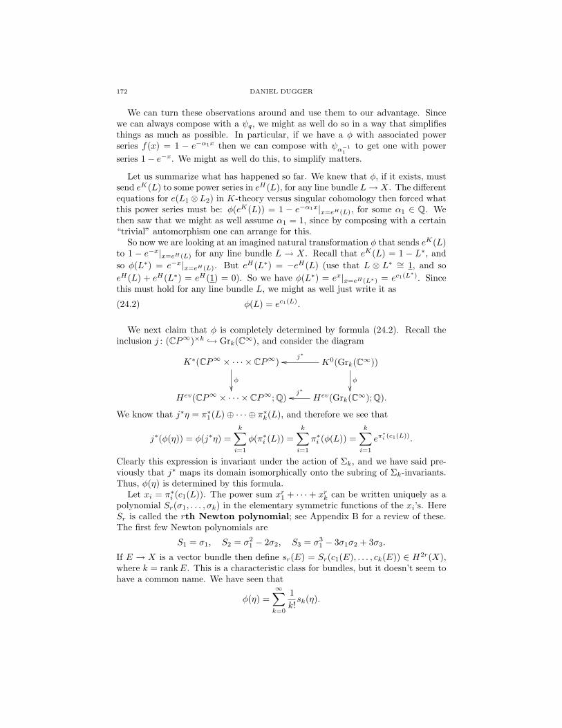
172 DANIEL DUGGER
We can turn these observations around and use them to our advantage. Sincewe can always compose with a ψq, we might as well do so in a way that simplifiesthings as much as possible. In particular, if we have a φ with associated powerseries f(x) = 1 − e−α1x then we can compose with ψα−1
1to get one with power
series 1− e−x. We might as well do this, to simplify matters.
Let us summarize what has happened so far. We knew that φ, if it exists, mustsend eK(L) to some power series in eH(L), for any line bundle L→ X. The differentequations for e(L1⊗L2) in K-theory versus singular cohomology then forced whatthis power series must be: φ(eK(L)) = 1 − e−α1x|x=eH(L), for some α1 ∈ Q. Wethen saw that we might as well assume α1 = 1, since by composing with a certain“trivial” automorphism one can arrange for this.
So now we are looking at an imagined natural transformation φ that sends eK(L)to 1 − e−x|x=eH(L) for any line bundle L → X. Recall that eK(L) = 1 − L∗, andso φ(L∗) = e−x|x=eH(L). But eH(L∗) = −eH(L) (use that L ⊗ L∗ ∼= 1, and soeH(L) + eH(L∗) = eH(1) = 0). So we have φ(L∗) = ex|x=eH(L∗) = ec1(L
∗). Sincethis must hold for any line bundle L, we might as well just write it as
φ(L) = ec1(L).(24.2)
We next claim that φ is completely determined by formula (24.2). Recall theinclusion j : (CP∞)×k → Grk(C∞), and consider the diagram
K∗(CP∞ × · · · × CP∞)
φ
K0(Grk(C∞))
φ
j∗oo
Hev(CP∞ × · · · × CP∞; Q) Hev(Grk(C∞); Q).j∗oo
We know that j∗η = π∗1(L)⊕ · · · ⊕ π∗k(L), and therefore we see that
j∗(φ(η)) = φ(j∗η) =k∑i=1
φ(π∗i (L)) =k∑i=1
π∗i (φ(L)) =k∑i=1
eπ∗i (c1(L)).
Clearly this expression is invariant under the action of Σk, and we have said pre-viously that j∗ maps its domain isomorphically onto the subring of Σk-invariants.Thus, φ(η) is determined by this formula.
Let xi = π∗i (c1(L)). The power sum xr1 + · · ·+ xrk can be written uniquely as apolynomial Sr(σ1, . . . , σk) in the elementary symmetric functions of the xi’s. HereSr is called the rth Newton polynomial; see Appendix B for a review of these.The first few Newton polynomials are
S1 = σ1, S2 = σ21 − 2σ2, S3 = σ3
1 − 3σ1σ2 + 3σ3.
If E → X is a vector bundle then define sr(E) = Sr(c1(E), . . . , ck(E)) ∈ H2r(X),where k = rankE. This is a characteristic class for bundles, but it doesn’t seem tohave a common name. We have seen that
φ(η) =∞∑k=0
1k!sk(η).
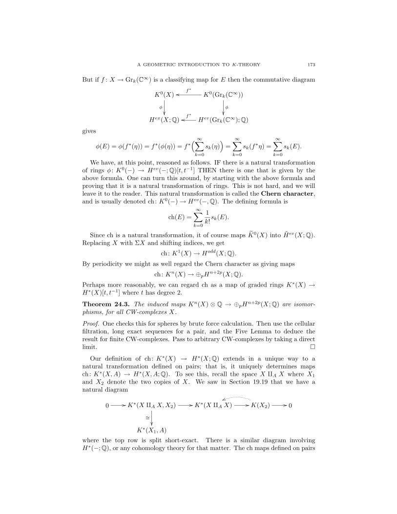
A GEOMETRIC INTRODUCTION TO K-THEORY 173
But if f : X → Grk(C∞) is a classifying map for E then the commutative diagram
K0(X)
φ
K0(Grk(C∞))
φ
f∗oo
Hex(X; Q) Hev(Grk(C∞); Q)f∗oo
gives
φ(E) = φ(f∗(η)) = f∗(φ(η)) = f∗( ∞∑k=0
sk(η))
=∞∑k=0
sk(f∗η) =∞∑k=0
sk(E).
We have, at this point, reasoned as follows. IF there is a natural transformationof rings φ : K0(−) → Hev(−; Q)[t, t−1] THEN there is one that is given by theabove formula. One can turn this around, by starting with the above formula andproving that it is a natural transformation of rings. This is not hard, and we willleave it to the reader. This natural transformation is called the Chern character,and is usually denoted ch: K0(−)→ Hev(−,Q). The defining formula is
ch(E) =∞∑k=0
1k!sk(E).
Since ch is a natural transformation, it of course maps K0(X) into Hev(X; Q).Replacing X with ΣX and shifting indices, we get
ch: K1(X)→ Hodd(X; Q).
By periodicity we might as well regard the Chern character as giving maps
ch: Kn(X)→ ⊕pHn+2p(X; Q).
Perhaps more reasonably, we can regard ch as a map of graded rings K∗(X) →H∗(X)[t, t−1] where t has degree 2.
Theorem 24.3. The induced maps Kn(X) ⊗ Q → ⊕pHn+2p(X; Q) are isomor-phisms, for all CW-complexes X.
Proof. One checks this for spheres by brute force calculation. Then use the cellularfiltration, long exact sequences for a pair, and the Five Lemma to deduce theresult for finite CW-complexes. Pass to arbitrary CW-complexes by taking a directlimit.
Our definition of ch: K∗(X) → H∗(X; Q) extends in a unique way to anatural transformation defined on pairs; that is, it uniquely determines mapsch: K∗(X,A) → H∗(X,A; Q). To see this, recall the space X qA X where X1
and X2 denote the two copies of X. We saw in Section 19.19 that we have anatural diagram
0 // K∗(X qA X,X2) //
∼=
K∗(X qA X) // K(X2)vv
// 0
K∗(X1, A)
where the top row is split short-exact. There is a similar diagram involvingH∗(−; Q), or any cohomology theory for that matter. The ch maps defined on pairs

174 DANIEL DUGGER
(Y, ∅) then uniquely determines a map ch: K∗(XqAX,X2)→ H∗(XqAX,X2; Q),and therefore a map ch: K∗(X,A)→ H∗(X,A; Q).
This raises the following interesting question. Suppose E• is a complex of vec-tor bundles on X that is exact on A. Then ch([E•]) is a well-defined element ofH∗(X,A; Q). How does one describe what this element is? We will return to thisquestion in the future. ?????
The existence of the Chern character, as a multiplicative natural transforma-tion between cohomology theories, immediately has an interesting and unexpectedconsequence:
Proposition 24.4. For any n ≥ 1, the image of ch: K0(S2n) → Hev(S2n; Q)is precisely Hev(S2n; Z). Consequently, if X is any (2n − 1)-connected space andE → X is a complex vector bundle then cn(E) ∈ H2n(X; Z) is a multiple of (n−1)!.
Proof. For the first statement recall that K0(S2n) is generated by β×n where β =1−L ∈ K0(S2). We can compute that ch(β) = 1−ch(L) = 1−(1+c1(L)) = −c1(L),but this is a generator of H2(S2; Z). Multiplicativity of the Chern character gives
ch(β×n) =(ch(β)
)×n = c1(L)×n,
but the nth external product of a generator for H2(S2; Z) gives a generator ofH2n(S2n; Z). This completes the proof of the first statement.
Note that if E → S2n is a complex vector bundle then ch(E) = 1n! · sn(E). The
Newton identities from Lemma B.1 show that sn(E) = (−1)n+1n · cn(E), sincein this case c1(E), . . . , cn−1(E) must all vanish. The fact that ch takes its imagein H2n(S2n; Z) then shows that ncn(E)
n! is integral; that is, cn(E) is a multiple by(n− 1)!.
Finally, let X be any (2n−1)-connected space. Replacing X by a weakly equiva-lent space, we can assume X has a cell structure with no cells of degree smaller than2n; that is, the 2n-skeleton is a wedge of 2n-spheres. Consider the cofiber sequence∨S2n → X → Q where C is the cofiber, and the induced maps in cohomology:
· · · ⊕K0(S2n)oo
ch
K0(X)oo
ch
K0(C)oo
ch
· · ·oo
· · · ⊕Hev(S2n; Q)oo Hev(X; Q)j∗oo Hev(C; Q)oo · · ·oo
We know by the commutativity of the diagram that j∗(chn(E)) lies in⊕Hev(S2n; Z). But since H2n(C; Q) = 0 the map j∗ is injective in degree 2n,and it is easy to see that (j∗)−1(H2n(∨S2n; Z)) = H2n(X; Z) (if a cellular 2n-cochain takes integral values on all of the 2n-cells, it is integral). So chn(E) isan integral class. The same computation as in the previous paragraph shows thatchn(E) = ± cn(E)
(n−1)! , and this completes the proof.
The space CP 1 is a complex manifold whose underlying topological manifold isS2. Can any other spheres be given the structure of a complex manifold? Clearlythis is only interesting for the even spheres. A simple corollary of the previousresult rules out almost all possibilities:

A GEOMETRIC INTRODUCTION TO K-THEORY 175
Corollary 24.5. If n ≥ 4 then there is no complex structure on S2n. Even more,there is no complex vector bundle whose underlying real bundle is the tangent bundleTS2n .
Proof. The second statement clearly implies the first. Let T = TS2n and supposethat T has a complex structure. By Proposition 24.4 we know that cn(T ) is amultiple of (n− 1)! in H2n(S2n; Z). But cn(T ) is the Euler class of the underlyingreal bundle, and therefore it is twice a generator since χ(S2n) = 2. This impliesthat 2
(n−1)! is an integer, which clearly cannot happen if n ≥ 4.
Remark 24.6. It is also know that S4 is not a complex manifold; we will give aproof in Example 25.16 below, using the Todd genus. Whether or not S6 admitsthe structure of complex manifold is an open problem.
We close this section with an example showing how the Chern character can helpus carry out the calculation of K-groups. This example will play an important rolewhen we study the Atiyah-Hirzebruch spectral sequence.
Example 24.7. Recall that CP 2 is the mapping cone on the Hopf map η : S3 → S2.Since the suspension of η is 2-torsion (π4(S3) ∼= Z/2), a choice of null-homotopyfor η 2 gives a map f : Σ3RP 2 → S3 which coincides with η when restricted to thebottom cell. Let X be the cofiber of f ; this is a cell complex with a 3-cell, a 5-cell,and a 6-cell. The 5-skeleton of X is ΣCP 2. Our goal will be to compute the groupsK∗(X). [Note: This choice of X, which seemingly has come out of nowhere, ismotivated by the fact that this is in some sense the smallest space for which K∗(X)and H∗(X) have different orders—see Remark 29.19 for a deeper perspective.]
There are two cofiber sequences that we can exploit: S3 → X → Σ4RP 2 andΣCP 2 → X → S6. We leave it to the reader to compute that K0(RP 2) = Z/2 andK1(RP 2) = 0, using that RP 2 is the cofiber of 2 : S1 → S1. Using this, the firstcofiber sequence gives
0 K0(S3) K0(X)oo Z/2oo Zoo K1(X)oo 0.oo
Note that we immediately deduce K1(X) ∼= Z, and K0(X) is either 0 or Z/2.However, it is not clear how to analyze the map Z → Z/2. The second cofibersequence gives
0 K0(X)oo Zoo Z2oo K1(X)oo 0oo
where the map Z2 → Z is the connecting homomorphism δ : K−1(ΣCP 2) →K0(S6). Again, we are left with the task of determining this map; agreementwith the previous (partial) calculation demands that the cokernel either be 0 orZ/2, and we need to determine which one. The good news is that because thedomain and target are both torsion-free, there is a chance that the Chern characterwill give us the information we need. We will examine the commutative square
Z2∼= // K−1(ΣCP 2)
δK //
ch
K0(S6)ch
∼= // Z
Hodd(ΣCP 2; Q)δH // Hev(S6; Q).

176 DANIEL DUGGER
The two Chern characters are injective because they are rational isomorphisms andthe domains are torsion-free.
Recall that K0(CP 2) = Z[Y ]/(Y 3) where Y = 1 − L. Let u be the standardgenerator for H2(CP 2), so that c1(L) = −u. We have
ch(Y ) = 1− ch(L) = 1− (1− u+ u2
2 ) = u− u2
2 , ch(Y 2) = ch(Y )2 = u2.
Write Y1 and Y2 for the suspensions of Y and Y 2, lying in K1(ΣCP 2); likewise,write u1 and u2 for the suspensions of u and u2 in H∗(ΣCP 2; Z). Compatibility ofthe Chern character with suspension shows that
ch(Y1) = u1 − u22 , ch(Y2) = u2.
We must next compute the images of these classes under δH . But this is easyfrom the long exact sequence for ΣCP 2 → X → S6: one finds that δ(u1) = 0 andδ(u2) is twice a generator in H6(S6). So the subgroup 〈δH(ch(Y1)), δH(ch(Y2))〉 ⊆H∗(S6; Q) equals the subgroup H6(S6; Z) ⊆ H6(S6; Q). Finally, recall from Propo-sition 24.4 that the image of ch: K0(S6)→ Hev(S6; Q) is also equal to H6(S6; Z).It follows that δK is surjective, and so the cokernel of δK is zero. This completesour calculation: K0(X) = 0.
To appreciate the significance of this example, note that Hev(X) ∼= Z/2 (concen-trated in degree 6) and Hodd(X) ∼= Z (concentrated in degree 3). The correspondingK-groups are K0(X) ∼= 0 and K0(X) ∼= Z. It is a general fact that all torsion-freesummands inH∗(X) will also appaear inK∗(X), as this follows from Theorem 24.3.But the present example demonstrates that the torsion subgroups of H∗(X) andK∗(X) can be quite different.
25. The Grothendieck-Riemann-Roch Theorem
As we present it here, the Grothendieck-Riemann-Roch (GRR) Theorem re-ally has two components: one that is purely topological, and one that is algebro-geometric. The topological part is a comparison between the complex-orientedstructures on K-theory and singular cohomology, and gives precise formulas forhow they line up under the Chern character. From the perspective that we haveadopted in these notes, this topological GRR theorem is fairly easy. The algebro-geometric component, on the other hand, is of a somewhat different nature; in ourpresentation it is a comparison between algebraic and topologicalK-theory, showingthat certain topologically-defined maps are compatible with purely algebraic onesthat at first glance appear quite different. This second part of the GRR theoremlets us see that certain algebraic constructions actually give topological invariants;the first part leads to precise (although often complex) topological formulas forthese invariants.
In the present section we discuss the topological GRR theorem and some of itsconsequences. The next section will deal with the algebro-geometric version.
25.1. The Todd class. We have seen that for a line bundle L→ X one has
ch(eK(L)) = (1− e−x)|x=eH(L).

A GEOMETRIC INTRODUCTION TO K-THEORY 177
The power series 1− e−x is a multiple of x, which means that the right-hand-sidecan be written as eH(L) multiplied by a ‘correction factor’:
ch(eK(L)) = eH(L) ·[1− e−x
x
]∣∣∣x=eH(L)
.
It is useful to have a name for this correction factor; for historical reasons, the nameis actually attached to its inverse. We define the Todd class of L to be
Td(L) =( x
1− e−x)∣∣∣x=c1(L)
=(1− x
2 + x2
6 −x3
24 + · · ·)∣∣∣x=c1(L)
=(1 + x
2 + x2
12 −x4
720 + · · ·)∣∣∣x=c1(L).
The coefficients in this power series are related to Bernoulli numbers, and we referthe reader to Appendix A for a review of the basics about these. The Bernoullinumbers are defined by x
ex−1 =∑iBi
i! xi, and so we have
Td(L) =∑i
(−1)i Bi
i! c1(L)i.
Next observe that if E → X is a sum of line bundles L1 ⊕ · · · ⊕ Lk then
ch(eK(E)) = ch(eK(L1) · · · eK(Lk))
= ch(eK(L1)) · · · ch(eK(Lk))
= [eH(L1) · · · eH(Lk)] ·[1− e−x
x
]∣∣∣x=c1(L1)
· · ·[1− e−x
x
]∣∣∣x=c1(Lk)
= eH(E) ·∏i
[1− e−xx
]∣∣∣∣x=c1(Li)
.
It therefore makes sense to define Td(E) to be the inverse of the product in thefinal formula. More generally, if E is a bundle of rank k then the Todd class of Eis
Td(E) =k∏i=1
( xi1− e−xi
)where ci(E) = σi(x1, . . . , xk). In other words, take the expression on the rightand write each homogeneous piece as a polynomial in the elementary symmetricfunctions. Then replace those symmetric functions with the Chern classes of E,and one gets the Todd class. For example, if rankE = 2 then we would expand(
1 + x2 + x2
12 −x4
720 + · · ·)·(1 + y
2 + y2
12 −y4
720 + · · ·)
to get
1 + 12 (x+ y) + 1
12 (x2 + y2) + 14xy + x2y+xy2
24 − x4+y4
720 + x2y2
144 + · · ·and then write this as
1 + 12σ1 + 1
12 (σ21 − 2σ2) + 1
4σ2 + 124 (σ1σ2) + 1
720 (−σ41 + 4σ2
1σ2 + 3σ42).
Then replace each σi with ci(E) to get the formula for Td(E).The first few terms of the Todd class of an arbitrary bundle are
(25.2) Td(E) = 1 +c12
+c21 + c2
12+c1c224
+−c41 + 4c21c2 − c4 + c1c3 + 3c22
720+ · · ·
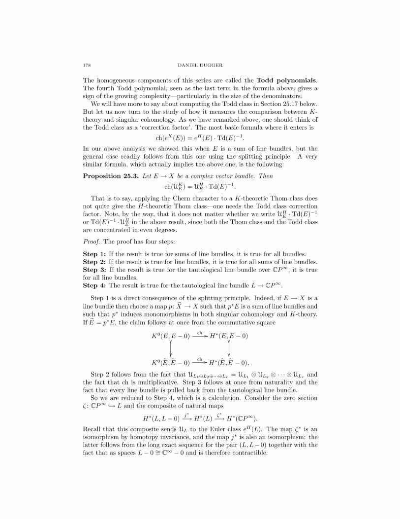
178 DANIEL DUGGER
The homogeneous components of this series are called the Todd polynomials.The fourth Todd polynomial, seen as the last term in the formula above, gives asign of the growing complexity—particularly in the size of the denominators.
We will have more to say about computing the Todd class in Section 25.17 below.But let us now turn to the study of how it measures the comparison between K-theory and singular cohomology. As we have remarked above, one should think ofthe Todd class as a ‘correction factor’. The most basic formula where it enters is
ch(eK(E)) = eH(E) · Td(E)−1.
In our above analysis we showed this when E is a sum of line bundles, but thegeneral case readily follows from this one using the splitting principle. A verysimilar formula, which actually implies the above one, is the following:
Proposition 25.3. Let E → X be a complex vector bundle. Then
ch(UKE ) = UHE · Td(E)−1.
That is to say, applying the Chern character to a K-theoretic Thom class doesnot quite give the H-theoretic Thom class—one needs the Todd class correctionfactor. Note, by the way, that it does not matter whether we write UHE · Td(E)−1
or Td(E)−1 ·UHE in the above result, since both the Thom class and the Todd classare concentrated in even degrees.
Proof. The proof has four steps:
Step 1: If the result is true for sums of line bundles, it is true for all bundles.Step 2: If the result is true for line bundles, it is true for all sums of line bundles.Step 3: If the result is true for the tautological line bundle over CP∞, it is truefor all line bundles.Step 4: The result is true for the tautological line bundle L→ CP∞.
Step 1 is a direct consequence of the splitting principle. Indeed, if E → X is aline bundle then choose a map p : X → X such that p∗E is a sum of line bundles andsuch that p∗ induces monomorphisms in both singular cohomology and K-theory.If E = p∗E, the claim follows at once from the commutative square
K0(E,E − 0)
ch // H∗(E,E − 0)
K0(E ,E − 0)
ch // H∗(E ,E − 0).
Step 2 follows from the fact that UL1⊕L2⊕···⊕Lr = UL1 ⊗ UL2 ⊗ · · · ⊗ ULr andthe fact that ch is multiplicative. Step 3 follows at once from naturality and thefact that every line bundle is pulled back from the tautological line bundle.
So we are reduced to Step 4, which is a calculation. Consider the zero sectionζ : CP∞ → L and the composite of natural maps
H∗(L,L− 0)j∗−→ H∗(L)
ζ∗−→ H∗(CP∞).
Recall that this composite sends UL to the Euler class eH(L). The map ζ∗ is anisomorphism by homotopy invariance, and the map j∗ is also an isomorphism: thelatter follows from the long exact sequence for the pair (L,L− 0) together with thefact that as spaces L− 0 ∼= C∞ − 0 and is therefore contractible.

A GEOMETRIC INTRODUCTION TO K-THEORY 179
Consider the two elements ch(UKL ) and UHL ·Td(L)−1 in H∗(L,L− 0). Applyingthe composite ζ∗ j∗ sends the first to ch(eK(L)), by naturality. Likewise, thesecond is sent to eH(L) · Td(L)−1. We have already computed that these twoimages are the same (indeed, this is how we started off this section); since ζ∗ j∗is an isomorphism this means ch(UKL ) = UHL · Td(L)−1.
25.4. The Grothendieck-Riemann-Roch Theorem for embeddings. Letj : X → Y be an embedding of complex manifolds of codimension c. We haveseen that one can construct a push-forward map j! : K∗(X)→ K∗+2c(Y ) and like-wise in any complex-oriented cohomology theory (for example, in H∗). We willtake advantage of Bott periodicity to write j! as a map K0(X)→ K0(Y ).
Consider the square
K0(X)j! //
ch
K0(Y )
ch
Hev(X; Q)
j! // Hev(Y ; Q).
This square does not commute; while this might seem strange, the point is justthat the j! maps are defined using Thom classes and ch doesn’t preserve these. Butsince ch almost preserves Thom classes, up to a correction factor, it follows thatthe above square almost commutes—up to the same factor. The precise result isas follows:
Proposition 25.5. Let j : X → Y be an embedding of complex manifolds. Thenfor any α ∈ K0(X) one has
ch(j!α) = j!(Td(NY/X)−1 · ch(α)).
Proof. Simply consider the diagram
K0(X) //
ch
K0(N,N − 0)
ch
K0(Y, Y −X)
ch
∼=oo // K0(Y )
ch
Hev(X) // Hev(N,N − 0) Hev(Y, Y −X) //∼=oo Hev(Y )
where all singular cohomology groups have rational coefficients. The left horizon-tal arrows are the Thom isomorphism maps, and so the leftmost square does notcommute; but the other two squares do. The compositions across the two rows arethe pushforward maps j! in K-theory and singular cohomology, respectively. Thedesired result is now an easy application of Proposition 25.3.
The next result records how the Chern character behaves on fundamental classes:
Corollary 25.6. If j : X → Y is an embedding of complex manifolds thench([X]K) = j!(Td(NY/X)−1) = [X]H + (higher degree terms).
Proof. Recall that [X]K = j!(1), and so the first equality is just Proposition 25.5applied to α = 1. The second equality then follows directly from the fact thatthe Todd class of a bundle has the form 1 + higher degree terms together withj!(1) = [X]H .
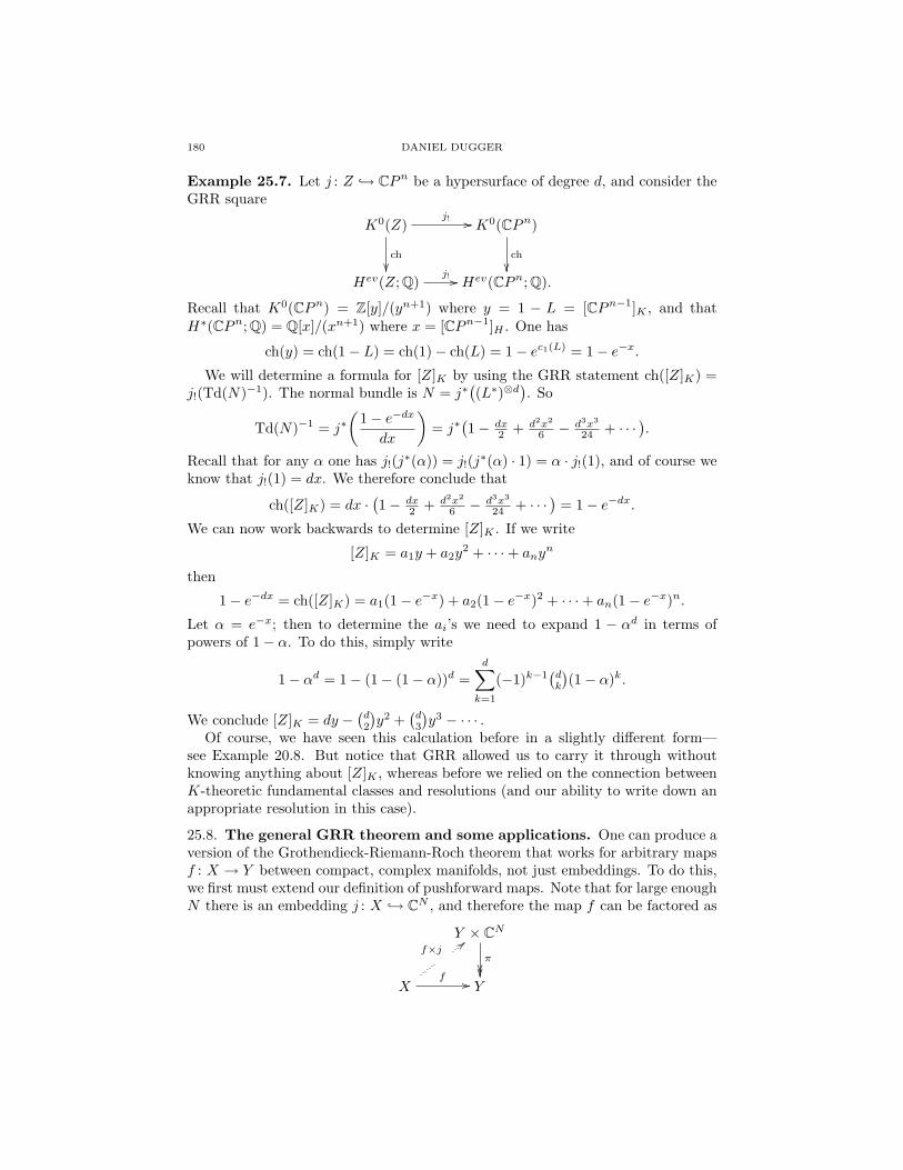
180 DANIEL DUGGER
Example 25.7. Let j : Z → CPn be a hypersurface of degree d, and consider theGRR square
K0(Z)j! //
ch
K0(CPn)
ch
Hev(Z; Q)
j! // Hev(CPn; Q).
Recall that K0(CPn) = Z[y]/(yn+1) where y = 1 − L = [CPn−1]K , and thatH∗(CPn; Q) = Q[x]/(xn+1) where x = [CPn−1]H . One has
ch(y) = ch(1− L) = ch(1)− ch(L) = 1− ec1(L) = 1− e−x.We will determine a formula for [Z]K by using the GRR statement ch([Z]K) =
j!(Td(N)−1). The normal bundle is N = j∗((L∗)⊗d
). So
Td(N)−1 = j∗(
1− e−dx
dx
)= j∗
(1− dx
2 + d2x2
6 − d3x3
24 + · · ·).
Recall that for any α one has j!(j∗(α)) = j!(j∗(α) · 1) = α · j!(1), and of course weknow that j!(1) = dx. We therefore conclude that
ch([Z]K) = dx ·(1− dx
2 + d2x2
6 − d3x3
24 + · · ·)
= 1− e−dx.We can now work backwards to determine [Z]K . If we write
[Z]K = a1y + a2y2 + · · ·+ any
n
then
1− e−dx = ch([Z]K) = a1(1− e−x) + a2(1− e−x)2 + · · ·+ an(1− e−x)n.Let α = e−x; then to determine the ai’s we need to expand 1 − αd in terms ofpowers of 1− α. To do this, simply write
1− αd = 1− (1− (1− α))d =d∑k=1
(−1)k−1(dk
)(1− α)k.
We conclude [Z]K = dy −(d2
)y2 +
(d3
)y3 − · · · .
Of course, we have seen this calculation before in a slightly different form—see Example 20.8. But notice that GRR allowed us to carry it through withoutknowing anything about [Z]K , whereas before we relied on the connection betweenK-theoretic fundamental classes and resolutions (and our ability to write down anappropriate resolution in this case).
25.8. The general GRR theorem and some applications. One can produce aversion of the Grothendieck-Riemann-Roch theorem that works for arbitrary mapsf : X → Y between compact, complex manifolds, not just embeddings. To do this,we first must extend our definition of pushforward maps. Note that for large enoughN there is an embedding j : X → CN , and therefore the map f can be factored as
Y × CN
π
X
f×j;;
f // Y
A GEOMETRIC INTRODUCTION TO K-THEORY 181
where π is projection onto the first factor. Let B ⊆ CN be a large disk that containsj(X). Now consider the composition
K0(X)j!−→ K0(Y × CN , Y × (CN −B)) ∼= K0(Y+ ∧ S2N ) ∼= K−2N (Y ).
Define this composite to be f!. It requires some checking to see that this is inde-pendent of the choice of factorization of f .
Example 25.9. It is interesting to take Y = ∗. Then the pushforward f! is a mapK0(X) → K−2d(∗) ∼= Z, so f!(1) gives an integer-valued invariant of the complexmanifold X. It is called the Todd genus of X, and we will denote it Td-genus(X).
Example 25.10. We can duplicate the above definition of f! in any complex-oriented cohomology theory, and therefore we get an associated genus for complexmanifolds (taking values in the coefficient ring of the theory). For singular coho-mology let us call this the H-genus.
Note that if f : X → Y then f! is a map
f! : Hi(X)→ Hi+2(dimY−dimX)(Y ).
If Y is a point then f! sends Hi(X) to Hi−2 dimX(pt), and so this is the zero mapunless i = 2dimX. In that dimension the cohomology of X is Z, generated by [∗].But recall that [∗] = j!(1) for any inclusion j : ∗ → X, and so
f!([∗]) = f!(j!(1)) = (f j)!(1) = id!(1) = 1.
We have therefore shown that f! : H∗(X) → H∗(pt) sends an element α ∈ H∗(X)to the coefficient of [∗] appearing in its 2 dim(X)-dimensional homogeneous piece.Usually it will be convenient to just say “f!(α) is the top-dimensional piece of α”.
As far as the H-genus is concerned, recall that it equals f!(1) for f : X → ∗. Butthis will be zero unless X = ∗, in which case it is 1. So
H-genus(X) =
0 if dimX > 0,#X if dimX = 0.
This is somewhat of a silly invariant, but it is what the theory gives us.
For the proof of our general version of GRR we will need to know the Todd genusof CPn, so let us compute this next:
Example 25.11 (Todd genus of CPn). Recall that Td(E ⊕ F ) = Td(E) · Td(F ),and that 1⊕ TCPn ∼= (n+ 1)L∗. So
Td(TCPn) = Td(TCPn) · Td(1) = Td((n+ 1)L∗
)=[Td(L∗)
]n+1.
Recall that c1(L∗) = [CPn−1] ∈ H2(CPn). Call this generator x, for short. Then
Td(TCPn) =( x
1− e−x)n+1
=(1 +
x
2+x2
12− x4
720+ · · ·
)n+1
.
Let’s look at some examples. When n = 1 we have x2 = 0 and so Td(TCP 1) =1 + x. When n = 2 we have x3 = 0 and
Td(TCP 2) =(1 + x
2 + x2
12
)3
= 1 + 32x+ x2.
Finally, for n = 3 we have x4 = 0 and
Td(TCP 3) =(1 + x
2 + x2
12
)4
= 1 + 2x+ 116 x
2 + x3.

182 DANIEL DUGGER
One discernible pattern in these polynomials is that the leading coefficient is al-ways 1. This is an amusing exercise that we leave to the reader. It shows thatTd-genus(CPn) = 1 for all n.
Exercise 25.12. Complete the above example by proving that the coefficient ofxn in
(x
1−e−x
)n+1 is equal to 1, for all n. One method is to interpret the coefficientas a residue:
Resx=0
(1
(1−e−x)n+1
)= 1
2πi
∫C
1(1−e−x)n+1 dx
where C is a small counterclockwise circle around the origin. Use the substitutionz = 1− e−x to convert this to a different residue that is easily computed. You willneed to convince yourself that the mapping x 7→ 1− e−x takes C to another smallcounterclockwise loop around the ogigin.
Exercise 25.13. Let Z → CPn be a smooth hypersurface of degree d. Show that
Td-genus(Z) = d−(d2
)+(d3
)− · · ·+ (−1)n
(dn
).
Conclude that if d ≤ n then Td-genus(Z) = 1.
We now state the general GRR theorem:
Theorem 25.14 (Grothendieck-Riemann-Roch, full version). Let X and Y be com-pact, complex manifolds and let f : X → Y be a map. Then in the square
K0(X)f! //
ch
K0(Y )
ch
Hev(X; Q)
f! // Hev(Y ; Q).
one hasch(f!α) · Td(TY ) = f!(ch(α) · Td(TX))
for all α ∈ K0(X), where TX and TY are the tangent bundles of X and Y .
Exercise 25.15. Check that when X → Y is an embedding then the above versionof GRR is equivalent to the version given in Proposition 25.5.
Proof of Theorem 25.14. The proof is via the steps listed below. We will outlinearguments in each case, but leave some of the details to the reader.
Step 1: The result is true when f is an embedding.Step 2: The result is true when f is CPn → ∗.Step 3: The result is true when f is the projection Y ×CPn → Y , for any compactcomplex manifold Y .Step 4: The result is true in general.
Step 1 was handled in Proposition 25.5. Step 2 is just a computation, whereone computes both sides of the GRR formula and sees that they are the same.Use that K0(CPn) is generated by the classes [CP i]. For the left side of GRR usethat [CP i] is mapped to 1 via f!, as Td-genus(CP i) = 1. For the right side usethat ch([CP i]) = (1− e−x)n−i and compute that the coefficient of xn in the series(1 − e−x)n−i ·
(x
1−e−x
)n+1 is equal to 1. For this final piece use a method similarto what we did in Exercise 25.12 above.
A GEOMETRIC INTRODUCTION TO K-THEORY 183
For Step 3 consider the product map K0(Y ) × K0(CPN ) → K0(Y × CPN ).We claim that this is an isomorphism, for any CW -complex Y . Indeed, considerthe functors (X,A) 7→ K∗(X,A) ⊗ K0(CPN ) and (X,A) 7→ K∗(X × CPN , A ×CPN ). Our product map gives a natural transformation from the first to thesecond, and both functors are generalized cohomology theories (in the second casethis is automatic, but in the first case this uses that K0(CPN ) is free and thereforeflat). One readily checks that the comparison map is an isomorphism when (X,A) =(pt, ∅), and so it follows that it is an isomorphism for all CW -pairs (X,A).
To complete Step 3 it now suffices to verify the GRR formula on classes of theform α = (p1)∗(β) · (p2)∗(γ) where β ∈ K0(Y ), γ ∈ K0(CPN ), and p1 and p2 arethe projections of Y × CPN onto Y and CPN , respectively. Use the diagram
Y × CPNp2 //
p1
CPN
π1
Y
π2 // ∗and the formulas
(p1)![p∗1β · p∗2γ
]= β · (p1)!(p∗2γ) = β · π∗2
((π1)!γ
)(as well as the analog of this in singular cohomology), together with Step 2.
Finally, for Step 4 factor f : X → Y as Xj−→ Y × CPN π−→ Y where j is an
embedding and π is projection. Use the diagram
K0(X)j! //
ch
K0(Y × CPN )
ch
π! // K0(Y )
ch
H∗(X; Q)
j! // H∗(Y × CPN ; Q)π! // H∗(Y ; Q),
where the horizontal composites are f!. We established GRR for the two squares, bySteps 1 and 3. Deduce the general GRR by putting these two squares together.
To see one example of GRR, consider the case Y = ∗. Here the GRR the-orem says ch(f!(1)) = f!(Td(TX)). We will compute both sides independently,and then see what information this theorem is giving. On the left-hand-side,f!(1) = Td-genus(X) · 1 ∈ K0(∗) and so ch(f!(1)) = Td-genus(X) · 1 ∈ H0(pt; Q).
To analyze the right-hand-side we recall from Example 25.10 above thatf! : Hev(X) → Hev(pt) sends a class α to its top-dimensional piece (the compo-nent in dimension 2 dimX). So GRR says that
Td-genus(X) · [∗] = top-dimensional piece of Td(TX).
One of the surprises here is that the right-hand-side is not a priori an integermultiple of [∗]: recall that the definition of the Todd class contains complicateddenominators. The resulting integrality conditions can lead to some nonexistenceresults in topology, as demonstrated in the following example.
Example 25.16. We claim that there is no complex manifold whose underlyingtopological manifold is S4; said differently, the space S4 cannot be given a complexstructure. If S4 were a complex manifold then it would have a Todd genus, which
184 DANIEL DUGGER
we know will be an integer. But GRR tells us that the Todd genus is also the top-dimensional component of Td(T ), where T denotes the complex tangent bundleof our fictitious complex manifold. But c1(T ) = 0 because H2(S4) = 0, andc2(T ) = 2[∗] because c2(T ) is the Euler class and χ(S4) = 2. Plugging into (25.2)we find that Td(T ) = 1 + c2
12 and so the top-dimensional piece is 16 . As this is not
an integer, we have arrived at a contradiction.A similar argument shows that S4n is not a complex manifold for any n, although
to follow through with this we will need to get better at computing terms in theTodd class. We return to this problem in Proposition 25.23 below.
25.17. Computing the Todd class. Let a1, a2, . . . be indeterminates and writeQ(x) = 1 + a1x+ a2x
3 + · · · . Let
Q(x) = Q(x1, . . . , xn) = Q(x1)Q(x2) · · ·Q(xn)
where the xi’s are formal variables of degree 1. This gives us a power series thatis invariant under permutations of the xi’s, and so it may be written as a powerseries in the elementary symmetric functions σi = σi(x1, . . . , xn), 1 ≤ i ≤ n. Ourgoal will be to give a formula, in terms of the ai’s, for the coefficient of any givenmonomial m = σm1
1 · · ·σmnn .
Notice that the degree of m is m1 + 2m2 + · · ·+ nmn; call this number N . Thecoefficient of m in Q(x) will not involve any terms ai for i > N , so we might aswell just assume that ai = 0 for i > N . In this case write
Q(x) = 1 + a1x+ · · ·+ aNxN = (1 + t1x)(1 + t2x) · · · (1 + tNx
N )
as a formal factorization of Q(x) (or if you like, we are working in the algebraicclosure of Q(a1, . . . , an)). Then
Q(x) =N∏i=1
Q(xi) =N∏i=1
N∏j=1
(1 + tjxi).
The evident next step is to reverse the order of the products, so let
Qj =N∏i=1
(1 + tjxi) = 1 + tjσ1 + t2jσ2 + · · ·+ tNj σN
and observe that Q(x) =∏j Qj . Consider the process of multiplying out all factors
in
(1 + σ1t1 + · · ·+ σN tN1 ) · (1 + σ1t2 + · · ·+ σN t
N2 ) · · · (1 + σ1tN + · · ·+ σN t
NN ).
The first few terms are
1 + σ1[t1] + σ2[t21] + σ21 [t1t2] + σ3[t31] + σ1σ2[t1t22] + · · ·
where the bracket notation means to sum the terms in the ΣN -orbit of the monomialinside the brackets (see Appendix B). Each of these brackets is a polynomial in theti’s that is invariant under the symmetric group, and therefore can be written (in aunique way) as a polynomial in the ai’s. These are the desired coefficients of Q(x).The general result, whose proof has basically just been given, is the following:
Proposition 25.18. The coefficient of σm11 · · ·σmn
n in Q(x) is
[t1t2 · · · tm1t2m1+1 · · · t2m1+m2
t3m1+m2+1 · · · t3m1+m2+m3· · · tnm1+···+mn
].
A GEOMETRIC INTRODUCTION TO K-THEORY 185
The bracketed expression in the above result looks horrible, but it is simplerthan it looks. The subscripts can basically be ignored. The idea is to write down aproduct of powers of the ti’s where no index i appears more than once and wherethe number of ti’s raised to the kth power is mk. For example, here are a fewσ-monomials and their associated coefficients:
σ4 : [t41], σ1σ3 : [t1t32], σ2σ23 : [t21t
32t
33], σ1σ
24σ6 : [t1t42t
43t
64].
For Proposition 25.18 to be useful one has to write the bracketed expression asa polynomial in the elementary symmetric functions σi(t) = ai. This is, of course,an unpleasant process. One case where it is not so bad is for the power sum [tn1 ],since here we have the Newton polynomials Sn described in Appendix B.
Corollary 25.19. For any k ≥ 1, the coefficient of σk in Q(x) is Sk(a1, . . . , ak),where Sk is the kth Newton polynomial. By Proposition B.3 this is also equal tothe two expressions
(−1)k ·[coeff. of xk in 1− x d
dx
(logQ(x)
) ]= (−1)k−1 ·
[coeff. of xk−1 in
Q′(x)Q(x)
].
Now let us specialize to Q(x) = x1−e−x =
∑i(−1)i Bi
i! xi. Then writing
Q(x1, . . . , xn) as a power series in the elementary symmetric functions exactly yieldsan expression for the Todd class of a rank n vector bundle in terms of its Chernclasses. Let us apply Corollary 25.19 to this situation; to do so we must computeQ′(x)/Q(x). This is easy enough:
Q′(x) = 11−e−x − xe−x
(1−e−x)2 = 1xQ(x)− e−x
1−e−xQ(x) =(
1x + 1− 1
1−e−x
)·Q(x)
and so1− xQ
′(x)Q(x) = 1− x
(1x + 1− 1
1−e−x
)= −x+Q(x).
Specializing Corollary 25.19 to the present situation now gives:
Corollary 25.20. Let E → X be a rank n vector bundle. Then for any 2 ≤ k ≤ n,the coefficient of ck in the formula for Td(E) is equal to Bk
k! , whereas the coefficientof c1 is −B1
1! = 12 .
Remark 25.21. Note that the above calculation reveals an interesting propertyof the coefficients of x
1−e−x : when you put them into the Newton polynomials Skthe output is unaltered, at least for k ≥ 2. That is, if x
1−e−x =∑i aix
i thenSk(a1, . . . , ak) = ak for k ≥ 2. For example, S4 = a4
1 − 4a21 + 4a1a3 + 2aa2 − 4a4
and the first few coeffcients of x1−e−x are 1
2 , 112 , 0, and − 1
720 . Some grade-schoolarithmetic checks that indeed
S4( 12 ,
112 , 0,−
1720 ) = − 1
720 .
But this is hardly obvious from just looking at the formula for S4.
25.22. An application of GRR. The following proposition is (mostly) weakerthan what we proved back in Corollary 24.5. Still, we offer it as a sample applicationof the Todd genus.
Proposition 25.23. No sphere S4n admits the structure of a complex manifold.
186 DANIEL DUGGER
Proof. Assume S4n is a complex manifold. Then it has a Todd genus, which isnecessarily an integer by definition. This will be the coefficient of [∗] in the topcomponent of the Todd class Td(T ), where T denotes the complex tangent bundleto S4n. To compute this Todd class directly from its definition, first note thatci(T ) = 0 for i < 2n, because H2i(S4n) = 0 in this range. We must also havecn(T ) = e(T ) = 2[∗], because the Euler characteristic of an even sphere equals 2.These facts let us easily write down Td(TS4n). Let us consider some examples ofthis.
When n = 1 we would have Td(TS4) = 1 + c212 . The Todd genus of S4 would
then be 212 , which is not an integer. When n = 2 we would have Td(TS8) = 1− c4
720 ,and so the Todd genus of S8 would be − 2
720 ; again, not an integer. These examplesgive the general idea, and the denominators only get worse as n gets larger.
To be specific, one will have TdS4n = 1 +Mc2n where M is a mystery numberthat must be computed from the definition of the Todd class. It is a consequence ofCorollary 25.20 that M = B2n
(2n)! . The Todd genus of S4n will then be 2 ·B2n/(2n)!.By Theorem A.5 the number 3 divides the lowest-terms-denominator of B2n, andso this expression cannot be an integer. This is our contradiction.
Remark 25.24. Notice why our proof of Proposition 25.23 does not extend tocover spheres S4n+2: the Chern class c2n+1 does not appear by itself in the formulafor the Todd class, because the odd Bernoulli numbers are zero. If S4n+2 has acomplex structure one can conclude that its Todd genus is zero, but this by itselfdoes not produce a contradiction.
25.25. The arithmetic genus. We now discuss the problem of computing theTodd genus for smooth algebraic subvarieties Z → CPn. We will see that it can bedescribed entirely in terms of algebro-geometric data. This material foreshadowsmuch of what we do in Section 26.
Let p : CPn → ∗ and q : Z → ∗ be the squash maps, and consider the composition
K0(Z)j!−→ K0(CPn) p!−→ K0(pt).
The composite is q! and therefore sends 1 to Td-genus(Z) · [∗]. On the other hand,if we write
j!(1) = [Z] = an−1[CPn−1] + an−2[CPn−2] + · · ·+ a0[CP 0]
then since p!([CPn−i]) = Td-genus(CPn−i) · [∗] = [∗] we have
p!(j!(1)) = (an−1 + an−2 + · · ·+ a0)[∗].So Td-genus(Z) =
∑i ai.
Recall that knowing [Z] is the same as knowing the Hilbert polynomial of Z. Wewish to ask the question: how can the Todd genus be extracted from the Hilbertpolynomial? To answer this, start by recalling the diagram
K0alg(CP
n)φ
∼=//
∼=
K0(CPn)
Ggrd(C[x0, . . . , xn])/〈[C]〉 // Hilb // Q[s]
from Section 20.18. The image of the function Hilb is the Z-submodule of Q[s]generated by
(s+nn
),(s+n−1n−1
), . . . ,
(s0
). If one takes [CPn−i] ∈ K0(CPn) and pushes
A GEOMETRIC INTRODUCTION TO K-THEORY 187
it around the diagram, we have seen in Section 20.18 that the corresponding Hilbertpolynomial is
(s+n−in−i
).
The Todd genus can be thought of as the unique function K0(CPn)→ Z sendingall the classes [CPn−i] to 1. We look for a similar function im(Hilb)→ Z that sends(s+n−in−i
)to 1, for all i. A moment’s thought shows that the map “evaluate at s = 0”
has this property. We have therefore proven the following:
Proposition 25.26. Let Z → CPn be an algebraic subvariety. Then the Toddgenus of Z is HilbZ(0).
In algebraic geometry, the invariant HilbZ(0) is sometimes called the arithmeticgenus. So we have proven that the arithmetic genus and Todd genus coincide.
Remark 25.27. Many authors use the term arithmetic genus for the invariant(−1)dimZ(HilbZ(0) − 1). This is the definition in both [H] and [GH], for exam-ple. Obviously the two definitions carry the same information, and the differencebetween them is only a matter of “normalization”. The invariant HilbZ(0) is some-times called the Hirzebruch genus, or the holomorphic Euler characteristic (seeSection ??? below for more information about this).
25.28. Fundamental classes and the Todd genus. Again let Z → CPn be acomplex submanifold of codimension c and consider the fundamental class [Z] ∈K0(CPn). Write
[Z] = an−c[CPn−c] + an−c−1[CPn−c−1] + · · ·+ a0[CP 0].
We have seen that an−c is the degree of Z, which has a simple geometric interpre-tation: it is the number of intersection points of Z with a generic linear subspace ofdimension c. But the question remains as to how to give a geometric interpretationfor the other ai’s. We will now explain how the Todd genus gives an answer this(although perhaps not an entirely satisfactory one).
As we saw in the last section, Td-genus(Z) =∑
0≤i ai. But note that multiplyingthe equation for [Z] by [CPn−1] gives [Z]·[CPn−1] = an−c[CPn−c−1]+· · ·+a1[CP 0]and therefore
Td-genus(Z ∩ CPn−1) =∑1≤i
ai.
Here Z ∩CPn−1 indicates the intersection of Z with a generic hyperplane in CPn.Likewise we have [Z] · [CPn−j ] = an−c[CPn−c−j ] + · · ·+ aj [CP 0], and hence
Td-genus(Z ∩ CPn−j) =∑j≤i
ai.
So the partial sums∑j≤i ai for j = 0, 1, . . . , n− c are the same as the Todd genera
of Z,Z ∩CPn−1, . . . , Z ∩CP c. (This gives another explanation for why an−c is thedegree of Z). We immediately obtain the formulas
ai = Td-genus(Z ∩ CPn−i)− Td-genus(Z ∩ CPn−i−1),(25.29)
where again the intersections are interpreted to be generic. This is our desiredgeometric description of the ai’s. Note, however, that whether or not this is indeed“geometric” depends on whether one feels that this adjective applies to the Toddgenus.
188 DANIEL DUGGER
26. The algebro-geometric GRR theorem
Let X be a compact complex manifold and E → X a complex vector bundle.If π denotes the projection X → ∗ then we get an element π!([E]) ∈ K0(pt) = Z.This gives an integer-valued invariant of the bundle E, which we will call the Toddnumber of E. We will write it as
Td-numX(E) = π!([E]).
The topological GRR theorem identifies this number as ΘX(Td(TX) · ch(E)), andso we can calculate it in terms of the Chern classes of E and TX . Note that theTodd number of the trivial bundle 1 is the Todd genus of X.
If X is an algebraic variety and E → X is an algebraic vector bundle then thereis another way to compute the Todd number of E, in terms of algebro-geometricinvariants. This identification of invariants is an example of the algebro-geometricGRR theorem. Although the theorem covers far more than just the Todd number,we will concentrate on this special case before stating the more general result.
26.1. Sheaf cohomology. As we saw in ???? the algebraic vector bundle E → Xgives rise to an associated coherent sheaf on the Zariski space XZar. We also callthis sheaf E, by abuse. Modern algebraic geometry shows how to obtain sheafcohomology groups Hi(X;E). The general theory is technical (although not in-credibly hard), and would take too long to recount here; the level of abstractionand technicality is roughly comparable to that of singular cohomology. But just asin the latter case, there are methods for computing the sheaf cohomology groupsthat do not require the high-tech definitions.
Suppose we have a Zariski open cover Uα of X with the property that eachUα is affine, and moreover assume that each iterated intersection Uα1 ∩ · · · ∩Uαk
isaffine (for each k ≥ 1). Write Γ(Uα, E) for the algebraic sections of E defined overUα. Then we may form the Cech complex
0→⊕α
Γ(Uα, E)→⊕α1,α2
Γ(Uα1 ∩ Uα2 , E)→ · · ·
and the sheaf cohomology group Hi(X;E) is just isomorphic to the ith cohomologygroup of this complex.
Example 26.2 (Cohomology of O(k) on CPn). Let x0, . . . , xn+1 be homogeneouscoordinates on CPn, and for each 0 ≤ j ≤ n let Uj ⊆ CPn be the open subschemedefined by xj 6= 0. Write Uj1···jr = Uj1 ∩ · · · ∩ Ujr , and note that all of these areaffine. Indeed, Uj is the spectrum of C[x0
xj, x1xj, . . . , xn
xj], Uj,k is the spectrum of the
localization of this ring at xk/xj , and so forth.Let S = C[x0, . . . , xn], regarded as a graded ring where all xi’s have degree 1.
Let Rj = Γ(Uj ,O) = C[x0xj, x1xj, . . . , xn
xj]. This is the degree zero homogeneous piece
of the localization Sxj. Further, observe that each O(k) is trivializable over Uj ,
and so Γ(Uj ,O(k)) will be a free Rj-module of rank 1. We can identify Γ(Uj ,O(k))with the degree k homogeneous component of the localization Sxj ; that is, it is theC-linear span of all monomials xa0
0 · · ·xann where aj ∈ Z and all other ai ≥ 0. This
is readily checked to coincide with the cyclic Rj-module xkjRj .The analogs of the above facts work for any open set Uj = Uj1 ∩ · · · ∩ Ujr .
The sections Γ(Uj ,O(k)) form the degree k homogeneous component of the ring
A GEOMETRIC INTRODUCTION TO K-THEORY 189
Sxj1 ···xjr. We want to examine the Cech complex C(U•,O(k)) for each value of k,
but it is more convenient to take the direct sum over all values for k and considerthem all at once.
For a collection of indices σ ⊆ 0, . . . , n let Sσ be the localization of S at theelement
∏i∈σ xi. Then consider the augmented Cech complex
C• : 0→ S → ⊕iSi → ⊕i<jSij → · · · → S01···n → 0
where the S is in degree −1 and where the differentials are all induced by theinclusions Sσ → Sσ′ for σ ⊆ σ′. That is to say, if we have a tuple α = (ασ ∈Sσ)#σ=r then dα is the tuple whose value at σ′ = i0, · · · , ir (with the entriesordered from least to greatest) is
(dα)σ′ =r∑
k=0
(−1)kαi0···bik···ir .The Cech complex for computing cohomology is obtained from C• by omitting theS in degree −1, but we will quickly see why it is convenient to have that S around.
It is easy to compute the cohomology group Hn(C•). The ring S01···bi···n isgenerated as a vector space by monomials xa0
0 · · ·xann where ai ≥ 0. So the image
of Cn−1 → Cn is the span of all monomials where some ai is nonnegative. Themonomials that are not in the image have the form x−1
0 · · ·x−1n · (x
−b00 · · ·x−bn
n )where all bi ≥ 0. So Hn(C•) only has terms in degree k ≤ −(n + 1), and in sucha degree the group is isomorphic to S−k−(n+1)(Cn+1). This computation will besubsumed by the more general one in the next paragraph, but it is useful to seethis particular case by itself.
To compute the cohomology of C• in all dimensions it is useful to regard S, andeach of its localizations, as multigraded by the group Zn+1 (by the multidegrees ofmonomials). The maps in the complex preserve this multigrading, so we might aswell look at one multidegree a = (a0, . . . , an) ∈ Zn+1 at a time. Let τ = i0, . . . , iube the complete list of indices for which ai < 0. Note that Sσ is zero in multidegreea unless σ ⊇ τ : that is, we will only have monomials of multidegree a if we haveinverted the xi’s for i ∈ τ . It is not hard to check that C•
a (the portion of C• inmultidegree a) coincides with the augmented simplicial chain complex for ∆n−#τ
with coefficients in C. The point is that the rings Sσ that are nonzero in degreea correspond to precisely those σ that contain τ , and these correspond in turnto subsets of 0, 1, . . . , n + 1 − τ . Subsets of 0, 1, . . . , n + 1 − τ also index thesimplices of ∆n−#τ , and we leave it to the reader to verify that the complexes doindeed coincide.
The augmented simplicial cochain complex for ∆n−#τ has zero cohomology ex-cept in one extreme case—for when #τ = n + 1 we have the augmented cochaincomplex of the emptyset, and this has a single Z in its cohomology. This cor-responds to those multidegrees a in which all ai < 0; for these the total degreesatisfies
∑ai ≤ −(n+ 1).
We have seen that C• is exact except in cohomological degree n, and there weget a single copy of C in every multidegree a for which
∑ai ≤ −(n+ 1). So for a
fixed integral degree k ≤ −(n+1) the kth homogeneous component of Hn(C) is theC-linear span of monomials xa where all ai < 0 and
∑ai = k. This is what we saw
earlier in the argument as well, and it gives us that Hn(C)k ∼= S−k−(n+1)(Cn+1).
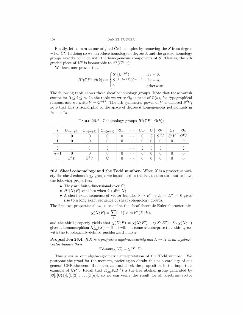
190 DANIEL DUGGER
Finally, let us turn to our original Cech complex by removing the S from degree−1 of C•. In doing so we introduce homology in degree 0, and the graded homologygroups exactly coincide with the homogeneous components of S. That is, the kthgraded piece of H0 is isomorphic to Sk(Cn+1).
We have now proven that
Hi(CPn;O(k)) ∼=
Sk(Cn+1) if i = 0,S−k−(n+1)(Cn+1) if i = n,
0 otherwise.
The following table shows these sheaf cohomology groups. Note that these vanishexcept for 0 ≤ i ≤ n. In the table we write Ok instead of O(k), for typographicalreasons, and we write V = Cn+1. The dth symmetric power of V is denoted SdV ;note that this is isomorphic to the space of degree d homogeneous polynomials inx0, . . . , xn.
Table 26.2. Cohomology groups Hi(CPn;O(k))
i O−(n+3) O−(n+2) O−(n+1) O−n · · · O−1 O O1 O2 O3
0 0 0 0 0 · · · 0 C S1V S2V S3V1 0 0 0 0 · · · 0 0 0 0 0...
......
...... · · ·
......
......
...n−1 0 0 0 0 · · · 0 0 0 0 0n S2V S1V C 0 · · · 0 0 0 0 0
26.3. Sheaf cohomology and the Todd number. When X is a projective vari-ety the sheaf cohomology groups we introduced in the last section turn out to havethe following properties:
• They are finite-dimensional over C;• Hi(X;E) vanishes when i > dimX;• A short exact sequence of vector bundles 0 → E′ → E → E′′ → 0 gives
rise to a long exact sequence of sheaf cohomology groups.The first two properties allow us to define the sheaf-theoretic Euler characteristic
χ(X;E) =∑i
(−1)i dimHi(X;E).
and the third property yields that χ(X;E) = χ(X;E′) + χ(X;E′′). So χ(X;−)gives a homomorphism K0
alg(X)→ Z. It will not come as a surprise that this agreeswith the topologically-defined pushforward map π!:
Proposition 26.4. If X is a projective algebraic variety and E → X is an algebraicvector bundle then
Td-numX(E) = χ(X;E).
This gives us our algebro-geometric interpretation of the Todd number. Wepostpone the proof for the moment, prefering to obtain this as a corollary of ourgeneral GRR theorem. But let us at least check the proposition in the importantexample of CPn. Recall that K0
alg(CPn) is the free abelian group generated by
[O], [O(1)], [O(2)], . . . , [O(n)]; so we can verify the result for all algebraic vector
A GEOMETRIC INTRODUCTION TO K-THEORY 191
bundles E by checking it for these particular n+ 1 cases. Luckily we have alreadycomputed the vector spaces Hi(CPn;O(k)). From Table 26.1 we find that
χ(CPn;O(k)) =
dimSkCn+1 if k ≥ 0,0 if −n ≤ k < 0,(−1)n dimS−k−(n+1)Cn+1 if k < −n.
We leave the reader to check that all three cases in the above formula can be unifiedinto the simple statement χ(CPn;O(k)) =
(n+kn
).
It remains to compute the Todd number of O(k). We use the by-now-familiartechnique from Exercise 25.12:
ΘX
[Td(TX) · ch(O(k))
]= Θn
[(x
1−e−x
)n+1 · ekx]
= Resx=0
(1
1−e−x
)n+1 · ekx dx
= Resz=0
(1
zn+1 · 1(1−z)k+1 dz
)= Θn
((1− z)−(k+1)
)= (−1)n
(−(k+1)n
)=(n+kn
).
Note that the substitution z = 1− e−x was used for the third equality.
27. Formal group laws and complex-oriented cohomology theories
28. Algebraic cycles on complex varieties
Note: The material in this section requires the Atiyah-Hirzebruch spectral se-quence from Section 29 below.
Let X be a smooth, projective algebraic variety over C. Every smooth subvarietyZ of codimension q has a fundamental class [Z] ∈ H2q(X; Z). In fact the smoothnessof Z is not needed here: every subvariety Z → X of codimension q has such afundamental class. This can be proven either by using resolution of singularietiesor by more naive methods—we will explain below.
Define H2qalg(X; Z) ⊆ H2q(X; Z) to be the subgroup generated by the fundamen-
tal classes of all algebraic subvarieties. How large are these “algebraic” parts of theeven cohomology groups? Are there examples of varieties X for which the algebraicpart does not equal everything?
The answer to the latter question is provided by Hodge theory: yes, there doexist varieties X where not all of the even cohomology is algebraic. Hodge theorygives a decomposition of the cohomology groups Hn(X; C) ∼= ⊕p+q=nHp,q(X), andthe algebraic classes all lie in the Hi,i pieces. The (even-dimensional) cohomologyis entirely algebraic only when Hp,q = 0 for p 6= q and p+ q even. But it is knownthat for an elliptic curve E one has H1,0 = C = H0,1, and so for E × E one getsH2,0(E × E) ∼= C ∼= H0,2(E × E). So not all of H2(E × E) is algebraic.
The problem with Hodge theory is that it cannot see any torsion classes, as thecoefficients of the cohomology groups need to be C. Could it be true that torsioncohomology classes are always algebraic? A classical theorem of Lefschetz, reprovedby Hodge, says that this holds for classes in H2. But for higher cohomology groupsthe answer is again no, and the first proof was given by Atiyah and Hirzebruch[AH2]. There are three basic components to their proof:
192 DANIEL DUGGER
(1) Every algebraic class must survive the Atiyah-Hirzebruch spectral sequence.The vanishing of the differentials therefore gives a sequence of obstructions fora given cohomology class to be algebraic.
(2) The differentials in the spectral sequence can be analyzed in terms of cohomol-ogy operations. On a pe-torsion class the first nonzero differential is d2p−1 andcoincides with the operation −βP 1.
(3) A clever construction of Serre’s shows how to obtain smooth algebraic varietieswhose cohomology contains that of BG through a range of dimensions. Usingthis, one readily finds smooth varieties with even-dimensional, p-torsion coho-mology classes for which βP 1 does not vanish; such a class cannot be algebraic.
The Atiyah-Hirzebruch proof is no longer the most efficient way to obtain condi-tions for torsion classes to be algebraic. Resolution of singularities shows that everyalgebraic class is actually a pushforward of the fundamental class of a manifold—i.e., every algebraic class lifts into complex cobordism. In the 1950s Thom hadalready obtained some necessary conditions for such a lifting to exist, in terms ofSteenrod operations. Via this method K-theory is not needed at all, and moreoverThom’s theory yields a stronger set of conditions. Note that resolution of singular-ities was not provided by Hironaka until 1964, and so of course was not availableat the time of [AH2].
Despite the modern shortcomings of Atiyah and Hirzebruch’s method, we willspend this section describing it in detail. It sheds some light on the relationshipbetween K-theory and singular cohomology, and also offers some neat observationsabout algebraic varieties.
Remark 28.1. We should mention that [AH2] treats the case of analytic cycles inaddition to algebraic cycles. The proofs are essentially the same, with one or twokey differences. We will not cover the material on analytic cycles here.
Remark 28.2. The modern Hodge conjecture states that any class α ∈ H2n(X; Q)whose image in H2n(X; C) lies in the Hodge group Hn,n(X) is necessarilyalgebraic—that is, it lies in the subgroup H2n(X; Q)alg. When Hodge originallyraised this question he did not explicitly specify rational coefficients. Since any tor-sion class in H2n(X; Z) would map to zero in H2n(X; C), and therefore lie insideHn,n(X), an integral version of the Hodge conjecture would imply that all torsionclasses are algebraic. One of the main points of [AH2] was to demonstrate that thisintegral form of the Hodge conjecture does not hold.
28.3. Fundamental classes for subvarieties. If X is a smooth algebraic varietyand Y ⊆ X is a smooth subvariety of codimension q then we have seen that complexorientability yields a fundamental class [Y ] ∈ H2q(X) and a relative fundamentalclass [Y ]rel ∈ H2q(X,X−Y ). This comes about by choosing a tubular neighborhoodU of Y that is homeomorphic to the normal bundle, and using the isomorphisms
H2q(X,X − Y ) ∼= H2q(U,U − Y ) ∼= H2q(N,N − 0).
Assuming Y is connected it follows that H2q(X,X − Y ) ∼= Z (by Thom isomor-phism), and [Y ]rel is defined to be the image of the Thom class UN ∈ H2q(N,N−0).The fundamental class [Y ] is just the image of [Y ]rel underH∗(X,X−Y )→ H∗(X).Note that the argument shows that choice of U and homeomorphism U ∼= N to beirrelevant: there are only two generators in H2q(X,X − Y ), and ???
We aim to show the existence of fundamental classes [Y ] even when the subvarietyY is not smooth.
A GEOMETRIC INTRODUCTION TO K-THEORY 193
Lemma 28.4. Let X be a smooth algebraic variety and let W → Y → X be subva-rieties. Assume that Y has codimension q inside of X, and that W has codimensionat least one inside of Y .(a) H∗(X)→ H∗(X − Y ) is an isomorphism for ∗ ≤ 2q − 2.(b) H∗(X,X − Y )→ H∗(X −W,X − Y ) is an isomorphism for ∗ ≤ 2q.(c) If Y is irreducible then H2q(X,X − Y ) ∼= Z.
Proof. First note that part (a) is true when Y is smooth, using the long exactsequence for the pair (X,X−Y ), the isomorphism H∗(X,X−Y ) ∼= H∗(N,N −0),and the Thom isomorphism theorem. For the general case, we can filter Y bysubvarieties
∅ ⊆ Y0 ⊆ Y1 ⊆ · · · ⊆ Ys = Y
where each Yi is the singular set of Yi+1 (so that Yi+1 − Yi is smooth). Since Y0 issmooth, we can assume by induction that H∗(X)→ H∗(X−Yi) is an isomorphismfor ∗ ≤ 2(codimYi)− 2. Now look at the composition
H∗(X)→ H∗(X − Yi)→ H∗(X − Yi+1) = H∗((X − Yi)− (Yi+1 − Yi)).
Since Yi+1 − Yi is smooth in X − Yi, the second map is an isomorphism for∗ ≤ 2(codimYi+1) − 2. It follows that the composite is an isomorphism for∗ ≤ 2(codimYi+1)− 2 as well, and now the desired result follows by induction.
Part (b) follows from part (a) via the long exact sequences
· · · // H∗−1(X − Y ) // H∗(X,X − Y ) // H∗(X) // H∗(X − Y ) // · · ·
· · · // H∗−1(X − Y )
∼=
OO
// H∗(X −W,X − Y )
OO
// H∗(X −W )
j∗
OO
// H∗(X − Y ) //
∼=
OO
· · ·
By (a) the map labelled j∗ is an isomorphism for ∗ ≤ 2q, and so the result followsby the five lemma.
Finally, for (c) we let Z be the singular set of Y . Then H2q(X,X − Y ) ∼=H2q(X−Z, (X−Z)− (Y −Z)) by (b). But Y −Z is a smooth subvariety of X−Zof codimension q, and it is connected because Y was irreducible. The remarks fromthe beginning of this section show that this cohomology group is isomorphic to Z,with generator [Y − Z]rel.
Now let Y → X be an algebraic subvariety of codimension q, and let Z be thesingular set. Since Y −Z is a smooth subvariety of X −Z, we have a fundamentalclass [Y −Z] ∈ H2q(X−Z). But by Lemma 28.4(a) the mapH2q(X)→ H2q(X−Z)is an isomorphism. We define [Y ] ∈ H2q(X) to be the preimage of [Y − Z] underthis map.
Define H∗alg(X) ⊆ H∗(X) to be the subgroup generated by the fundamental
classes of all the algebraic subvarieties of X.In the next section it will help to be able to focus on classes [Y ] where Y is
irreducible. To this end, the following is useful:
Lemma 28.5. If Y → X is a codimension q subvariety with irreducible componentsY1, . . . , Yk then [Y ] =
∑i[Yi] ????? The subgroup H∗
alg(X) is spanned by classes
Proof. ????
We need one more lemma before moving on:

194 DANIEL DUGGER
Proposition 28.6. Let M be a real manifold and let N → M be a codimensionk real submanifold with a tubular neighborhood. Then M − N → M is (k − 1)-connected.
Sketch. ????
28.7. Vanishing of differentials on algebraic classes. Let X be a smoothalgebraic variety, and let Y ⊆ X be subvariety. Let F• be a resolution of OY bylocally-free OX -modules, and write F• for the associated chain complex of complexvector bundles onX. Then [F•] defines a class inK0(X,X−Y ) which we will denote[Y ]K,rel. Note that when Y is smooth this agrees with the relative fundamentalclass provided by the complex orientation of K-theory, by Theorem 18.8.
Proposition 28.8. One has ch([Y ]K,rel) = [Y ]H,rel + higher order terms.
Proof. We first prove this when Y is smooth. If N denotes the normal bundle for Yin X, then the result will follow once we know ch(UKN ) = UHN +higher order terms—for both [Y ]K,rel and [Y ]H,rel are obtained from the Thom classes by applyingnatural maps. However, we have already seen in our discussion of Riemann-Rochthat the complete formula is in fact
ch(UKN ) = UHN · Td(N)−1
(see Proposition 25.3). Now just observe that Td(N)−1 = 1 + higher order terms.Now let Y be arbitrary. Let Z be the singular locus, and the q denote the
codimension of Y . Consider the diagram
K0(X,X − Y )j∗ //
ch
K0(X − Z,X − Y )
ch
H∗(X,X − Y )
j∗ // H∗(X − Z,X − Y ).
Both maps j∗ are simply restriction to an open set, and so j∗([Y ]K,rel) = [Y −Z]K,rel and j∗([Y ]H,rel) = [Y − Z]H,rel. By Lemma 28.4(b) the bottom map is anisomorphism for ∗ ≤ 2q. So the desired result for Y follows from the correspondingresult for Y − Z, which has already been proven because Y − Z is smooth inX − Z.
Theorem 28.9. Let X be a smooth algebraic variety, and let Y ⊆ X be a sub-variety. Then [Y ]H survives the Atiyah-Hirzebruch spectral sequence; that is, alldifferentials vanish on this class.
Proof. This is now easy. The class [Y ]H is the image of [Y ]H,rel under the naturalmap H∗(X,X − Y ) → H∗(X). By naturality of the Atiyah-Hirzebruch spectralsequence, it suffices to show that all differentials on [Y ]H,rel are zero. This followsfrom Proposition 28.8 and ????.
Corollary 28.10. Let X be a smooth algebraic variety, and let p be a fixed prime.If a pe-torsion class u ∈ Hev(X) is algebraic then βP 1(u) = 0.
Proof. Immediate from Theorem 28.9 and Proposition 29.20(b).

A GEOMETRIC INTRODUCTION TO K-THEORY 195
28.11. Construction of varieties with non-algebraic cohomology classes.At this point our job is to construct a smooth, projective algebraic variety X thathas a class u ∈ Hev(X) for which βP 1x 6= 0, for some prime p. Such a class cannotbe algebraic by Corollary 28.10. It turns out that p can be any prime we like—thatis, for any given p we can find an example of an X and a u. Moreover, u can betaken to lie in degree 4. The construction comes out of the following three results:
Theorem 28.12 (Serre). Let G be a finite group and let n ≥ 0.(a) There exists a linear action of G on a projective space CPN together with
an n-dimensional, closed, smooth subvariety X → CPN which is a completeintersection, invariant under G, and has G acting freely.
(b) If X is a variety having the properties in (a), then its homotopy (n− 1)-type isthe same as that of K(Z, 2)×BG.
Corollary 28.13. Let G be a finite group and let n ≥ 0. There exists an n-dimensional, smooth, projective variety whose (n − 1)-homotopy type is the sameas that of K(Z, 2)×BG.
Proposition 28.14. Let p be a prime. Then there exists a finite group G and aclass u ∈ H4(BG; Z) that is killed by p and is such that βP 1(u) 6= 0.
We postpone the proofs for one moment so that we can observe the immediateconsequence:
Corollary 28.15 (Atiyah-Hirzebruch). Fix a prime p. There exists a smooth,projective, complex algebraic variety X and a class u ∈ Hev(X) that is killed by psuch that u is not algebraic.
Proof. By Proposition 28.14 there exists a finite group G and a p-torsion class u ∈H4(BG; Z) such that βP 1(u) 6= 0. By Theorem 28.12 there is a smooth, projectivevariety X whose (2p+ 4)-type is the same as K(Z, 2)×BG. But then H∗(BG; Z)is a direct summand of H∗(X) up through dimension 2p + 4. By Corollary 28.10the class in H4(X) corresponding to u cannot be algebraic.
Theorem 28.12 requires some algebraic geometry, but the proofs of both Corol-lary 28.13 and Proposition 28.14 are purely topological. We tackle these in reverseorder:
Proof of Proposition 28.14. We start by considering p = 2 (the odd case turns outto be extremely similar). As a first attempt we might try to take G = Z/2. ThenBZ/2 = RP∞, H∗(RP∞; Z/2) = Z/2[x], and H∗(RP∞; Z) = Z/2[x2]. Unfortu-nately Sq3 = β Sq2 vanishes on all the integral classes, by an easy calculation.
Next look at B(Z/2×Z/2) = RP∞×RP∞. The mod 2 cohomology is Z/2[x, y],and the integral cohomology is the subring consisting of all elements whose Bock-stein vanishes. Such elements of course include all polynomials in x2 and y2, butit also includes θ = x2y + xy2 = β(xy). In fact all the elements of the integralcohomology look like x2iy2j · θ. Another easy calculation shows that Sq3 appliedto such an element is x2iy2j Sq3(θ), and Sq3(θ) = x4y2 + x2y4 6= 0. This gives uslots of classes that are not killed by Sq3, however they are all in odd dimensions.So this still doesn’t solve our problem.
In the preceding paragraph, the reason things didn’t work ultimately came downto the fact that β(xy) had odd dimension. This gets fixed once we move to

196 DANIEL DUGGER
B(Z/2 × Z/2 × Z/2). The mod 2 cohomology is Z/2[x, y, z], and again the in-tegral cohomology is the subring consisting of the elements where the Bocksteinvanishes. One such element is θ = β(xyz) = x2yz + xy2z + xyz2. It is easy to cal-culate that Sq3 θ = x4y2z+x4yz2 + · · · 6= 0. So finally we have an even-dimensionalintegral cohomology class where Sq3 vanishes.
The argument for odd primes works the same way. Recall that H∗(BZ/p; Z/p) =Λ(u)⊗ Fp[v], with β(u) = v and P 1(v) = vp. Take G = Z/p× Z/p× Z/p and lookat θ = β(u1u2u3) ∈ H4(BG; Z). A simple calculation shows that βP 1(θ) 6= 0.
Next, the corollary to Serre’s theorem:
Proof of Corollary 28.13. Let X → CPN be the subvariety provided by Theo-rem 28.12. Since X → CPN is a complete intersection, the strong form of theWeak Lefschetz Theorem ??? yields that X → CPN is an (n− 1)-equivalence. Letη → CPN be the tautological line bundle CN+1 − 0 → CPN . Note that G actson CN+1, and so G acts on the bundle η. Hence G acts on the pullback bundlej∗η → X. Since the action of G on X is free we get a line bundle (j ∗ η)/G→ X/Gwhich pulls back to j∗η along the projection X → X/G. Let the classifying mapfor this line bundle be X/G→ CP∞. The diagram
X //
CPN
X/G // CP∞
necessarily commutes up to homotopy, as the two compositions classify the samebundle j∗η. Since X → CPN is an (n − 1)-equivalence, so is the composite X →CP∞.
Consider the composite map X → X/G → CP∞. This is a G-equivariantmap, where the target is given the trivial G-action. Since the map is an (n − 1)-equivalence, the induced map on homotopy orbit spacesXhG → (CP∞)hG is also an(n− 1)-equivalence. (Recall that ZhG = (Z ×EG)/G. Crossing with EG preservesthe (n−1)-equivalence, and since Z×EG→ ZhG is a covering space it follows thatquotienting by G also preserves the (n − 1)-equivalence). But since the G-actionon X is free one has XhG ' X/G, and since the action on CP∞ is trivial one has(CP∞)hG ' CP∞ ×BG. This completes the proof.
Finally, we prove Serre’s theorem.
Proof of Theorem 28.12. We first give the proof for G = Z/2. Even though thegeneral case is basically the same, certain steps can be made more concrete byrestricting to this case.
Let C2M have coordinates x1, . . . , xM , y1, . . . , yM , and let G act trivially on thex’s and by negation on the y’s. Consider the induced action on P = P(C2M ) =CP 2M−1. The homogeneous coordinate ring is R = C[x1, . . . , xM , y1, . . . , yM ], andthe ring of invariants S = RG is the subring generated by the xi’s and the yiyj ’s(including i = j). An easy argument shows that every homogeneous element ofS having even degree is a polynomial in the elements xixj and yiyj . That is, ifS(2) ⊆ S is the C-linear span of all even-dimensional homogeneous elements thenS(2) is generated (as a subring) by elements of degree 2.
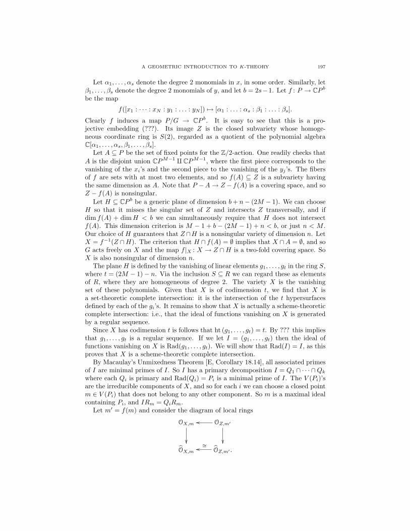
A GEOMETRIC INTRODUCTION TO K-THEORY 197
Let α1, . . . , αs denote the degree 2 monomials in x, in some order. Similarly, letβ1, . . . , βs denote the degree 2 monomials of y, and let b = 2s−1. Let f : P → CP bbe the map
f([x1 : · · · : xN : y1 : . . . : yN ]) 7→ [α1 : . . . : αs : β1 : . . . : βs].
Clearly f induces a map P/G → CP b. It is easy to see that this is a pro-jective embedding (???). Its image Z is the closed subvariety whose homoge-neous coordinate ring is S(2), regarded as a quotient of the polynomial algebraC[α1, . . . , αs, β1, . . . , βs].
Let A ⊆ P be the set of fixed points for the Z/2-action. One readily checks thatA is the disjoint union CPM−1 qCPM−1, where the first piece corresponds to thevanishing of the xi’s and the second piece to the vanishing of the yj ’s. The fibersof f are sets with at most two elements, and so f(A) ⊆ Z is a subvariety havingthe same dimension as A. Note that P −A→ Z − f(A) is a covering space, and soZ − f(A) is nonsingular.
Let H ⊆ CP b be a generic plane of dimension b+ n− (2M − 1). We can chooseH so that it misses the singular set of Z and intersects Z transversally, and ifdim f(A) + dimH < b we can simultaneously require that H does not intersectf(A). This dimension criterion is M − 1 + b − (2M − 1) + n < b, or just n < M .Our choice of H guarantees that Z∩H is a nonsingular variety of dimension n. LetX = f−1(Z ∩H). The criterion that H ∩ f(A) = ∅ implies that X ∩A = ∅, and soG acts freely on X and the map f |X : X → Z ∩H is a two-fold covering space. SoX is also nonsingular of dimension n.
The planeH is defined by the vanishing of linear elements g1, . . . , gt in the ring S,where t = (2M − 1)− n. Via the inclusion S ⊆ R we can regard these as elementsof R, where they are homogeneous of degree 2. The variety X is the vanishingset of these polynomials. Given that X is of codimension t, we find that X isa set-theoretic complete intersection: it is the intersection of the t hypersurfacesdefined by each of the gi’s. It remains to show that X is actually a scheme-theoreticcomplete intersection: i.e., that the ideal of functions vanishing on X is generatedby a regular sequence.
Since X has codimension t is follows that ht (g1, . . . , gt) = t. By ??? this impliesthat g1, . . . , gt is a regular sequence. If we let I = (g1, . . . , gt) then the ideal offunctions vanishing on X is Rad(g1, . . . , gt). We will show that Rad(I) = I, as thisproves that X is a scheme-theoretic complete intersection.
By Macaulay’s Unmixedness Theorem [E, Corollary 18.14], all associated primesof I are minimal primes of I. So I has a primary decomposition I = Q1 ∩ · · · ∩Qkwhere each Qi is primary and Rad(Qi) = Pi is a minimal prime of I. The V (Pi)’sare the irreducible components of X, and so for each i we can choose a closed pointm ∈ V (Pi) that does not belong to any other component. So m is a maximal idealcontaining Pi, and IRm = QiRm.
Let m′ = f(m) and consider the diagram of local rings
OX,m
OZ,m′oo
OX,m OZ,m′ .
∼=oo
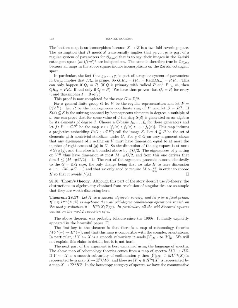
198 DANIEL DUGGER
The bottom map is an isomorphism because X → Z is a two-fold covering space.The assumption that H meets Z transversally implies that g1, . . . , gt is part of aregular system of parameters for OZ,m′ ; that is to say, their images in the Zariskicotangent space (m′)/(m′)2 are independent. The same is therefore true in OX,m,because all maps in the above square induce isomorphisms on the Zariski cotangentspace.
In particular, the fact that g1, . . . , gt is part of a regular system of parametersin OX,m implies that IRm is prime. So QiRm = IRm = Rad(IRm) = PiRm. Thiscan only happen if Qi = Pi (if Q is primary with radical P and P ⊆ m, thenQRm = PRm if and only if Q = P ). We have thus proven that Qi = Pi for everyi, and this implies I = Rad(I).
This proof is now completed for the case G = Z/2.For a general finite group G let V be the regular representation and let P =
P(VM ). Let R be the homogeneous coordinate ring of P , and let S = RG. IfS(d) ⊆ S is the subring spanned by homogeneous elements in degrees a multiple ofd, one can prove that for some value of d the ring S(d) is generated as an algebraby its elements of degree d. Choose a C-basis f0, . . . , fb for these generators andlet f : P → CP b be the map x 7→ [f0(x) : f1(x) : · · · : fb(x)]. This map inducesa projective embedding P/G → CP b; call the image Z. Let A ⊆ P be the set ofelements with nontrivial stabilizer under G. For g ∈ G an easy argument showsthat any eigenspace of g acting on V must have dimension equal to at most thenumber of right cosets of 〈g〉 in G. So the dimension of the eigenspace is at most#G/#〈g〉, and therefore is bounded above by #G/2. The eigenspaces of g actingon VM thus have dimension at most M · #G/2, and from this one derives thatdimA ≤ (M · #G/2) − 1. The rest of the argument proceeds almost identicallyto the G = Z/2 case, the only change being that we take H to have dimensionb+ n− (M ·#G− 1) and that we only need to require M > 2n
#G in order to chooseH so that it avoids f(A).
28.16. Thom’s theory. Although this part of the story doesn’t use K-theory, theobstructions to algebraicity obtained from resolution of singularities are so simplethat they are worth discussing here.
Theorem 28.17. Let X be a smooth algebraic variety, and let p be a fixed prime.If u ∈ Hev(X; Z) is algebraic then all odd-degree cohomology operations vanish onthe mod p reduction u ∈ Hev(X; Z/p). In particular, all the odd Steenrod squaresvanish on the mod 2 reduction of u.
The above theorem was probably folklore since the 1960s. It finally explicitlyappeared in the beautiful paper [T].
The first key to the theorem is that there is a map of cohomology theoriesMU∗(−)→ H∗(−), and that this map is compatible with the complex orientations.In particular, if Y → X is a smooth subvariety it sends [Y ]MU to [Y ]H . We willnot explain this claim in detail, but it is not hard.
The next part of the argument is best explained using the language of spectra.The above map of cohomology theories comes from a map of spectra MU → HZ.If Y → X is a smooth subvariety of codimension q then [Y ]MU ∈ MU2q(X) isrepresented by a map X → Σ2qMU , and likewise [Y ]H ∈ H2q(X) is represented bya map X → Σ2qHZ. In the homotopy category of spectra we have the commutative
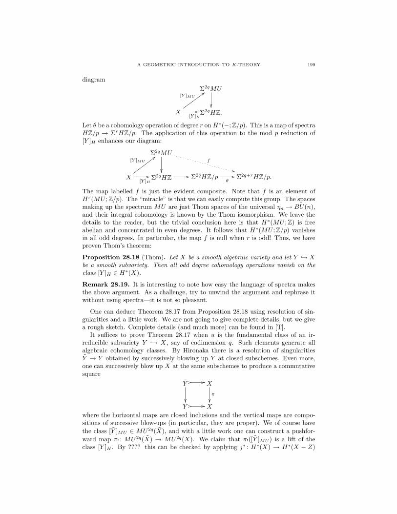
A GEOMETRIC INTRODUCTION TO K-THEORY 199
diagramΣ2qMU
X
[Y ]MU
;;vvvvvvvvv
[Y ]H
// Σ2qHZ.
Let θ be a cohomology operation of degree r onH∗(−; Z/p). This is a map of spectraHZ/p → ΣrHZ/p. The application of this operation to the mod p reduction of[Y ]H enhances our diagram:
Σ2qMU
f
++X
[Y ]MU
;;wwwwwwwww
[Y ]H
// Σ2qHZ // Σ2qHZ/pθ
// Σ2q+rHZ/p.
The map labelled f is just the evident composite. Note that f is an element ofHr(MU ; Z/p). The “miracle” is that we can easily compute this group. The spacesmaking up the spectrum MU are just Thom spaces of the universal ηn → BU(n),and their integral cohomology is known by the Thom isomorphism. We leave thedetails to the reader, but the trivial conclusion here is that H∗(MU ; Z) is freeabelian and concentrated in even degrees. It follows that H∗(MU ; Z/p) vanishesin all odd degrees. In particular, the map f is null when r is odd! Thus, we haveproven Thom’s theorem:
Proposition 28.18 (Thom). Let X be a smooth algebraic variety and let Y → Xbe a smooth subvariety. Then all odd degree cohomology operations vanish on theclass [Y ]H ∈ H∗(X).
Remark 28.19. It is interesting to note how easy the language of spectra makesthe above argument. As a challenge, try to unwind the argument and rephrase itwithout using spectra—it is not so pleasant.
One can deduce Theorem 28.17 from Proposition 28.18 using resolution of sin-gularities and a little work. We are not going to give complete details, but we givea rough sketch. Complete details (and much more) can be found in [T].
It suffices to prove Theorem 28.17 when u is the fundamental class of an ir-reducible subvariety Y → X, say of codimension q. Such elements generate allalgebraic cohomology classes. By Hironaka there is a resolution of singularitiesY → Y obtained by successively blowing up Y at closed subschemes. Even more,one can successively blow up X at the same subschemes to produce a commutativesquare
Y // //
X
π
Y // // X
where the horizontal maps are closed inclusions and the vertical maps are compo-sitions of successive blow-ups (in particular, they are proper). We of course havethe class [Y ]MU ∈ MU2q(X), and with a little work one can construct a pushfor-ward map π! : MU2q(X) → MU2q(X). We claim that π!([Y ]MU ) is a lift of theclass [Y ]H . By ???? this can be checked by applying j∗ : H∗(X) → H∗(X − Z)

200 DANIEL DUGGER
where Z is the singular set of Y and seeing that j∗(π!([Y ]MU )) = [Y − Z]. Thiscan in turn be deduced from an appropriate push-pull formula and the fact thatY − π−1(Y ) → Y − Z is a homeomorphism. In any case, if you accept this lastpoint then we now have the diagram
Σ2qMU
X
π!([Y ]MU );;vvvvvvvvv
[Y ]H
// Σ2qHZ
and at this point everything proceeds the same as before. This completes our sketchof a proof for Theorem 28.17.
Note that even with this approach, as opposed to the K-theory approach ofAtiyah-Hirzebruch, one still needs to gives examples of algebraic varieties withnontrivial odd-degree operations on even-dimensional cohomology classes. So thehard work that went on in Section 28.11 is still necessary.
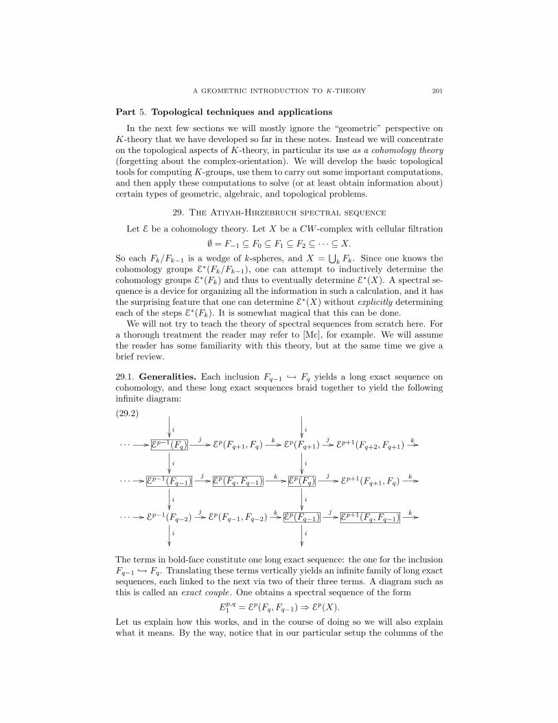
A GEOMETRIC INTRODUCTION TO K-THEORY 201
Part 5. Topological techniques and applications
In the next few sections we will mostly ignore the “geometric” perspective onK-theory that we have developed so far in these notes. Instead we will concentrateon the topological aspects of K-theory, in particular its use as a cohomology theory(forgetting about the complex-orientation). We will develop the basic topologicaltools for computing K-groups, use them to carry out some important computations,and then apply these computations to solve (or at least obtain information about)certain types of geometric, algebraic, and topological problems.
29. The Atiyah-Hirzebruch spectral sequence
Let E be a cohomology theory. Let X be a CW -complex with cellular filtration
∅ = F−1 ⊆ F0 ⊆ F1 ⊆ F2 ⊆ · · · ⊆ X.So each Fk/Fk−1 is a wedge of k-spheres, and X =
⋃k Fk. Since one knows the
cohomology groups E∗(Fk/Fk−1), one can attempt to inductively determine thecohomology groups E∗(Fk) and thus to eventually determine E∗(X). A spectral se-quence is a device for organizing all the information in such a calculation, and it hasthe surprising feature that one can determine E∗(X) without explicitly determiningeach of the steps E∗(Fk). It is somewhat magical that this can be done.
We will not try to teach the theory of spectral sequences from scratch here. Fora thorough treatment the reader may refer to [Mc], for example. We will assumethe reader has some familiarity with this theory, but at the same time we give abrief review.
29.1. Generalities. Each inclusion Fq−1 → Fq yields a long exact sequence oncohomology, and these long exact sequences braid together to yield the followinginfinite diagram:
i
i
· · · // Ep−1(Fq)
i
j // Ep(Fq+1, Fq)k // Ep(Fq+1)
i
j // Ep+1(Fq+2, Fq+1)k //
· · · // Ep−1(Fq−1)j //
i
Ep(Fq, Fq−1)k // Ep(Fq)
i
j // Ep+1(Fq+1, Fq)k //
· · · // Ep−1(Fq−2)j //
i
Ep(Fq−1, Fq−2)k // Ep(Fq−1)
i
j // Ep+1(Fq, Fq−1)k //
(29.2)
The terms in bold-face constitute one long exact sequence: the one for the inclusionFq−1 → Fq. Translating these terms vertically yields an infinite family of long exactsequences, each linked to the next via two of their three terms. A diagram such asthis is called an exact couple. One obtains a spectral sequence of the form
Ep,q1 = Ep(Fq, Fq−1)⇒ Ep(X).
Let us explain how this works, and in the course of doing so we will also explainwhat it means. By the way, notice that in our particular setup the columns of the

202 DANIEL DUGGER
diagram are eventually zero as one proceeds downward, because Fi = ∅ when i isnegative. Notice as well that if X = Fn for some value of n (so the filtration isfinite) then the columns stabilize when moving upwards.
(0). Here is the basic idea for how the spectral sequence operates. Consider anelement x ∈ Ep(Fq, Fq−1), and proceed as follows:
(i) Let x0 = kx.(ii) If j(x0) = 0 then x0 = i(x1) for some x1 ∈ Ep(Fq+1). We may then look at
jx1.(iii) If jx1 = 0 then x1 = i(x2) for some x2 ∈ Ep(Fq+2). We may then look at jx2.(iv) Continuing in this way, we get a sequence of “obstructions” jxu, u = 0, 1, 2, . . ..
Each one only exists if the previous one vanishes. Note that at each stage thevanishing of jxu doesn’t depend on the choice of xu; however, it may dependon the choice of xv made at some previous stage v < u. In this sense theobstructions are not unique: different choices of lifts may lead to differentobstructions later down the line.
(v) If we can make choices such that all of these obstructions vanish then we areable to lift kx arbitrarily far up in the diagram. If the filtration F• was finitethis means that we have produced an element of Ep(X); it turns out somethinglike this also works for infinite filtrations, although the resulting element ofEp(X) is only uniquely determined in good cases. The spectral sequence isa device for keeping track of these obstructions and liftings, and what theyultimately produce.
We will now go through all of the machinery needed to define and work with thespectral sequence associated to our exact couple.
(1). For 1 ≤ r ≤ ∞ write
Zp,qr = x ∈ Ep(Fq, Fq−1) | kx may be lifted at least r times under i.This is called the group of r-cycles in the spectral sequence. The phrasing isambiguous when r =∞, but we mean Zp,q∞ =
⋂r Z
p,qr . We also define Bp,qr ⊆ Zp,qr
to be the subgroup generated by all “obstructions” that arise from at most r − 1layers lower down in the diagram. To be precise, Bp,qr is spanned by the sets
ji−sk(Ep−1(Fq−s−1, Fq−s−2))
for 0 ≤ s ≤ r − 1. It is best to immediately forget this precise description and justremember the idea.
Notice that everything in Bp,qr maps to zero under k, and hence is contained inevery Zp,qs . That is, we have
0 = Bp,q0 ⊆ Bp,q1 ⊆ · · · ⊆ Bp,q∞ ⊆ Zp,q∞ ⊆ · · · ⊆ Zp,q2 ⊆ Zp,q1 ⊆ Zp,q0 = Ep(Fq, Fq−1).
Note that Bp,q∞ =⋃r B
p,qr and Zp,q∞ =
⋂r Z
p,qr .
(2). It as an easy exercise to prove that x ∈ Bp,qr if and only if x can be writtenas x = j(y1 + y2 + · · · + yr) for some yu’s such that iu(yu) = 0, for all u. As animmediate corollary, Bp,q∞ coincides with the image of j (or equivalently with thekernel of k).
Let x0 ∈ Ep(Fq) and assume that we lifted x0 a total of r times: that is, assumewe have chosen elements xu ∈ Ep(Fq+u) for 1 ≤ u ≤ r such that i(xu) = xu−1. Ifj(xr) ∈ Bs for some s then (using the result of the previous paragraph) there exists
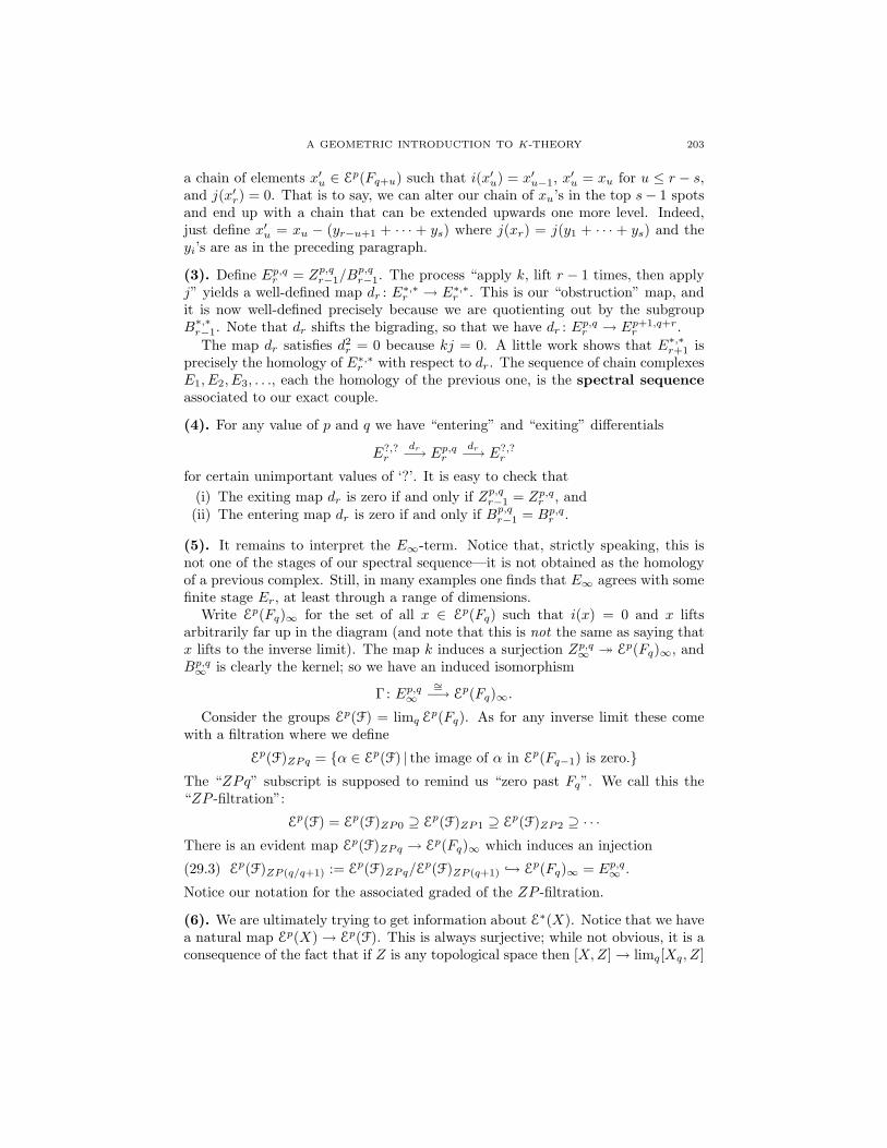
A GEOMETRIC INTRODUCTION TO K-THEORY 203
a chain of elements x′u ∈ Ep(Fq+u) such that i(x′u) = x′u−1, x′u = xu for u ≤ r − s,
and j(x′r) = 0. That is to say, we can alter our chain of xu’s in the top s− 1 spotsand end up with a chain that can be extended upwards one more level. Indeed,just define x′u = xu − (yr−u+1 + · · · + ys) where j(xr) = j(y1 + · · · + ys) and theyi’s are as in the preceding paragraph.
(3). Define Ep,qr = Zp,qr−1/Bp,qr−1. The process “apply k, lift r − 1 times, then apply
j” yields a well-defined map dr : E∗,∗r → E∗,∗r . This is our “obstruction” map, andit is now well-defined precisely because we are quotienting out by the subgroupB∗,∗r−1. Note that dr shifts the bigrading, so that we have dr : Ep,qr → Ep+1,q+r
r .The map dr satisfies d2
r = 0 because kj = 0. A little work shows that E∗,∗r+1 isprecisely the homology of E∗,∗r with respect to dr. The sequence of chain complexesE1, E2, E3, . . ., each the homology of the previous one, is the spectral sequenceassociated to our exact couple.
(4). For any value of p and q we have “entering” and “exiting” differentials
E?,?r
dr−→ Ep,qrdr−→ E?,?
r
for certain unimportant values of ‘?’. It is easy to check that(i) The exiting map dr is zero if and only if Zp,qr−1 = Zp,qr , and(ii) The entering map dr is zero if and only if Bp,qr−1 = Bp,qr .
(5). It remains to interpret the E∞-term. Notice that, strictly speaking, this isnot one of the stages of our spectral sequence—it is not obtained as the homologyof a previous complex. Still, in many examples one finds that E∞ agrees with somefinite stage Er, at least through a range of dimensions.
Write Ep(Fq)∞ for the set of all x ∈ Ep(Fq) such that i(x) = 0 and x liftsarbitrarily far up in the diagram (and note that this is not the same as saying thatx lifts to the inverse limit). The map k induces a surjection Zp,q∞ Ep(Fq)∞, andBp,q∞ is clearly the kernel; so we have an induced isomorphism
Γ: Ep,q∞∼=−→ Ep(Fq)∞.
Consider the groups Ep(F) = limq Ep(Fq). As for any inverse limit these comewith a filtration where we define
Ep(F)ZPq = α ∈ Ep(F) | the image of α in Ep(Fq−1) is zero.The “ZPq” subscript is supposed to remind us “zero past Fq”. We call this the“ZP -filtration”:
Ep(F) = Ep(F)ZP0 ⊇ Ep(F)ZP1 ⊇ Ep(F)ZP2 ⊇ · · ·There is an evident map Ep(F)ZPq → Ep(Fq)∞ which induces an injection
Ep(F)ZP (q/q+1) := Ep(F)ZPq/Ep(F)ZP (q+1) → Ep(Fq)∞ = Ep,q∞ .(29.3)
Notice our notation for the associated graded of the ZP -filtration.
(6). We are ultimately trying to get information about E∗(X). Notice that we havea natural map Ep(X)→ Ep(F). This is always surjective; while not obvious, it is aconsequence of the fact that if Z is any topological space then [X,Z]→ limq[Xq, Z]

204 DANIEL DUGGER
is surjective, which in turn is a routine application of the homotopy extensionproperty for cellular inclusions. Let
Ep(X)ZPq = ker(Ep(X)→ Ep(Fq−1)
)and note that we have a map of filtrations Ep(X)ZP• → Ep(F)ZP•. The map onassociated graded groups
Ep(X)ZP (q/q+1) → Ep(F)ZP (q/q+1)
is readily seen to be an isomorphism, for all q.
(7). If we are in “good” cases then the map in (29.3) will actually be an isomor-phism. The question is whether an element of Ep(Fq) that can be lifted arbitrarilyhigh in the diagram can also be lifted into the inverse limit—note that this is notautomatic! It might be possible that higher and higher liftings exist but not “coher-ently”; that is, to get a higher lifting one needs to change arbitrarily many elementslower down in the chain.
Fix a p and consider the following condition:
(SSCp) :There exists an N such that for all q the differentials entering andexiting the group Ep,qr are zero for all r ≥ N .
If this “Spectral Sequence Convergence Condition” holds then by (4) we knowZp,qN−1 = Zp,qr and Bp,qN−1 = Bp,qr for all r ≥ N . Therefore Zp,q∞ = Zp,qN−1, B
p,q∞ =
Bp,qN−1, and consequently Ep,q∞ = Ep,qN . These statements hold for all values of q. Sothe Ep,∗∞ groups coincide with the stable values of the Ep,∗r groups.
The convergence condition (SSCp) gives us one more important consequence,namely that the map of (29.3) is an isomorphism:
(SSCp)⇒[
Ep(F)ZP (q/q+1)∼= Ep,q∞ , for all q.
]To prove this, let x0 ∈ Ep(Fq)∞. Then there exist elements xu ∈ Ep(Fq+u) for1 ≤ u ≤ 2N uch that i(xu) = xu−1 for each u (nothing special about 2N is beingused here, it is just a convenient large number). The element j(x2N ) lies in B2N+1,which we have seen equals BN−1 by (SSCp). Therefore by (2) we may modify thexu’s in dimensions x2N , x2N−1, . . . , xN+3 in such a way that the chain extends toan x2N+1. It is important here that only the top N−2 elements are affected, for wecan now continue by induction and build an element of Ep(F) = lims Ep(Fs) thatmaps to x in Ep(Fq). This completes the proof.
To summarize, the statement that the spectral sequence “converges to Ep(X)”is usually interpreted to mean that
• The groups Ep,∗r stabilize, and equal Ep,∗∞ , at some value of r (usually onethat is independent of the grading ∗); and,
• The maps in (29.3) are isomorphisms, for all values of q.Under these conditions the stable values of the spectral sequence give the associatedgraded groups of the ZP -filtration on Ep(X). We have seen that (SSCp) impliesthis kind of convergence.
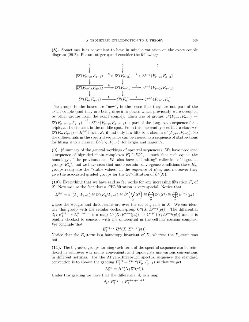
A GEOMETRIC INTRODUCTION TO K-THEORY 205
(8). Sometimes it is convenient to have in mind a variation on the exact couplediagram (29.2). Fix an integer q and consider the following:
...
...
...
Ep(Fq+2, Fq−1)k //
Ep(Fq+2)j //
Ep+1(Fq+3, Fq+2)
Ep(Fq+1, Fq−1)k //
Ep(Fq+1)j //
Ep+1(Fq+2, Fq+1)
Ep(Fq, Fq−1)k // Ep(Fq)
j // Ep+1(Fq+1, Fq)
The groups in the boxes are “new”, in the sense that they are not part of theexact couple (and they are being drawn in places which previously were occupiedby other groups from the exact couple). Each trio of groups Ep(Fq+r, Fq−1) →Ep(Fq+r−1, Fq−1)
jk−→ Ep+1(Fq+r, Fq+r−1) is part of the long exact sequence for atriple, and so is exact in the middle spot. From this one readily sees that a class u ∈Ep(Fq, Fq−1) = Ep,q1 lies in Zr if and only if u lifts to a class in Ep(Fq+r, Fq−1). Sothe differentials in the spectral sequence can be viewed as a sequence of obstructionsfor lifting u to a class in Ep(FN , Fq−1), for larger and larger N .
(9). (Summary of the general workings of spectral sequences). We have produceda sequence of bigraded chain complexes E∗,∗1 , E∗,∗2 , . . . such that each equals thehomology of the previous one. We also have a “limiting” collection of bigradedgroups E∗,∗∞ , and we have seen that under certain convergence conditions these E∞groups really are the “stable values” in the sequence of Er’s, and moreover theygive the associated graded groups for the ZP -filtration of E∗(X).
(10). Everything that we have said so far works for any increasing filtration F• ofX. Now we use the fact that a CW -filtration is very special. Notice that
Ep,q1 = Ep(Fq, Fq−1) ∼= Ep(Fq/Fq−1) ∼= Ep(∨α
Sq)∼=⊕α
Ep(Sq) ∼=⊕α
Ep−q(pt)
where the wedges and direct sums are over the set of q-cells in X. We can iden-tify this group with the cellular cochain group Cq(X;Ep−q(pt)). The differentiald1 : Ep,q1 → Ep+1,q+1
1 is a map Cq(X;Ep−q(pt)) → Cq+1(X;Ep−q(pt)) and it isreadily checked to coincide with the differential in the cellular cochain complex.We conclude that
Ep,q2∼= Hq(X;Ep−q(pt)).
Notice that the E2-term is a homotopy invariant of X, whereas the E1-term wasnot.
(11). The bigraded groups forming each term of the spectral sequence can be rein-dexed in whatever way seems convenient, and topologists use various conventionsin different settings. For the Atiyah-Hirzebruch spectral sequence the standardconvention is to choose the grading Ep,q1 = Ep+q(Fp, Fp−1) so that we get
Ep,q2 = Hp(X;Eq(pt)).
Under this grading we have that the differential dr is a map
dr : Ep,q2 → Ep+r,q−r+12 .
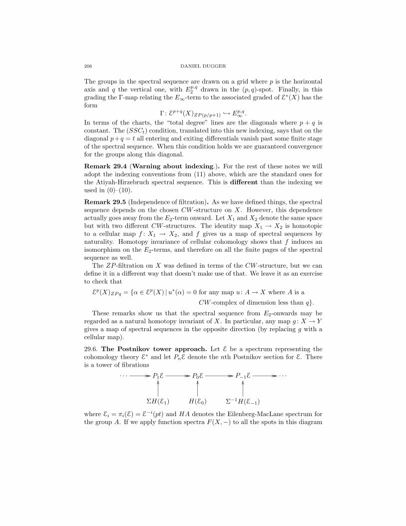
206 DANIEL DUGGER
The groups in the spectral sequence are drawn on a grid where p is the horizontalaxis and q the vertical one, with Ep,q2 drawn in the (p, q)-spot. Finally, in thisgrading the Γ-map relating the E∞-term to the associated graded of E∗(X) has theform
Γ: Ep+q(X)ZP (p/p+1) → Ep,q∞ .
In terms of the charts, the “total degree” lines are the diagonals where p + q isconstant. The (SSCt) condition, translated into this new indexing, says that on thediagonal p+q = t all entering and exiting differentials vanish past some finite stageof the spectral sequence. When this condition holds we are guaranteed convergencefor the groups along this diagonal.
Remark 29.4 (Warning about indexing.). For the rest of these notes we willadopt the indexing conventions from (11) above, which are the standard ones forthe Atiyah-Hirzebruch spectral sequence. This is different than the indexing weused in (0)–(10).
Remark 29.5 (Independence of filtration). As we have defined things, the spectralsequence depends on the chosen CW -structure on X. However, this dependenceactually goes away from the E2-term onward. Let X1 and X2 denote the same spacebut with two different CW -structures. The identity map X1 → X2 is homotopicto a cellular map f : X1 → X2, and f gives us a map of spectral sequences bynaturality. Homotopy invariance of cellular cohomology shows that f induces anisomorphism on the E2-terms, and therefore on all the finite pages of the spectralsequence as well.
The ZP -filtration on X was defined in terms of the CW -structure, but we candefine it in a different way that doesn’t make use of that. We leave it as an exerciseto check that
Ep(X)ZPq = α ∈ Ep(X) |u∗(α) = 0 for any map u : A→ X where A is a
CW -complex of dimension less than q.These remarks show us that the spectral sequence from E2-onwards may be
regarded as a natural homotopy invariant of X. In particular, any map g : X → Ygives a map of spectral sequences in the opposite direction (by replacing g with acellular map).
29.6. The Postnikov tower approach. Let E be a spectrum representing thecohomology theory E∗ and let PnE denote the nth Postnikov section for E. Thereis a tower of fibrations
· · · // // P1E // // P0E // // P−1E // // · · ·
ΣH(E1)
OO
H(E0)
OO
Σ−1H(E−1)
OO
where Ei = πi(E) = E−i(pt) and HA denotes the Eilenberg-MacLane spectrum forthe group A. If we apply function spectra F (X,−) to all the spots in this diagram
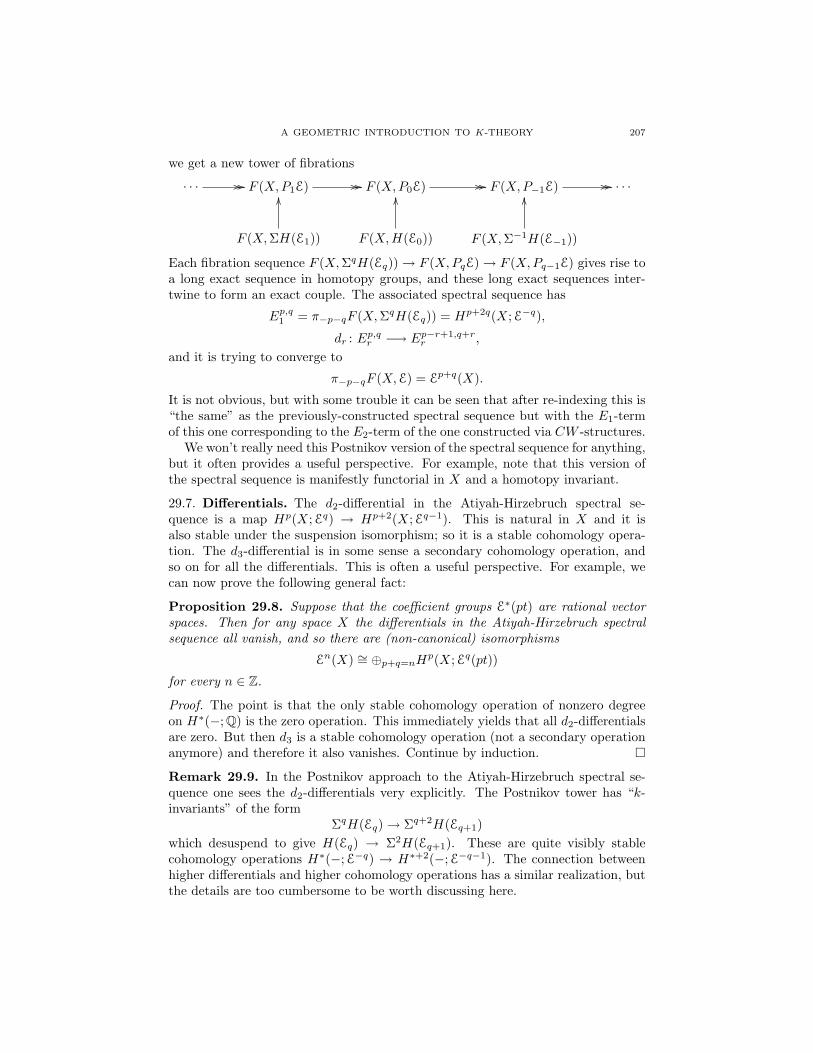
A GEOMETRIC INTRODUCTION TO K-THEORY 207
we get a new tower of fibrations
· · · // // F (X,P1E) // // F (X,P0E) // // F (X,P−1E) // // · · ·
F (X,ΣH(E1))
OO
F (X,H(E0))
OO
F (X,Σ−1H(E−1))
OO
Each fibration sequence F (X,ΣqH(Eq))→ F (X,PqE)→ F (X,Pq−1E) gives rise toa long exact sequence in homotopy groups, and these long exact sequences inter-twine to form an exact couple. The associated spectral sequence has
Ep,q1 = π−p−qF (X,ΣqH(Eq)) = Hp+2q(X;E−q),
dr : Ep,qr −→ Ep−r+1,q+rr ,
and it is trying to converge to
π−p−qF (X,E) = Ep+q(X).
It is not obvious, but with some trouble it can be seen that after re-indexing this is“the same” as the previously-constructed spectral sequence but with the E1-termof this one corresponding to the E2-term of the one constructed via CW -structures.
We won’t really need this Postnikov version of the spectral sequence for anything,but it often provides a useful perspective. For example, note that this version ofthe spectral sequence is manifestly functorial in X and a homotopy invariant.
29.7. Differentials. The d2-differential in the Atiyah-Hirzebruch spectral se-quence is a map Hp(X;Eq) → Hp+2(X;Eq−1). This is natural in X and it isalso stable under the suspension isomorphism; so it is a stable cohomology opera-tion. The d3-differential is in some sense a secondary cohomology operation, andso on for all the differentials. This is often a useful perspective. For example, wecan now prove the following general fact:
Proposition 29.8. Suppose that the coefficient groups E∗(pt) are rational vectorspaces. Then for any space X the differentials in the Atiyah-Hirzebruch spectralsequence all vanish, and so there are (non-canonical) isomorphisms
En(X) ∼= ⊕p+q=nHp(X;Eq(pt))
for every n ∈ Z.
Proof. The point is that the only stable cohomology operation of nonzero degreeon H∗(−; Q) is the zero operation. This immediately yields that all d2-differentialsare zero. But then d3 is a stable cohomology operation (not a secondary operationanymore) and therefore it also vanishes. Continue by induction.
Remark 29.9. In the Postnikov approach to the Atiyah-Hirzebruch spectral se-quence one sees the d2-differentials very explicitly. The Postnikov tower has “k-invariants” of the form
ΣqH(Eq)→ Σq+2H(Eq+1)which desuspend to give H(Eq) → Σ2H(Eq+1). These are quite visibly stablecohomology operations H∗(−;E−q) → H∗+2(−;E−q−1). The connection betweenhigher differentials and higher cohomology operations has a similar realization, butthe details are too cumbersome to be worth discussing here.
208 DANIEL DUGGER
It is worth observing that from the E2-term onward there are never any dif-ferentials emanating from the p = 0 line of the spectral sequence. For conve-nience assume X is connected and choose a cell structure on X where F0 = ∗.By the remarks in (8) above, such differentials would be the obstructions for aclass in Eq(F0, ∅) to lift to Eq(Fr, ∅); but such a lifting necessarily exists, be-cause F0 → Fr is split. Note that when X is connected Eq(X)ZP1 = Eq(X),and Eq(X)ZP (1/2) = Eq(X)/Eq(X) = Eq(pt), giving further confirmation that theE∞-term coincides with the E2-term on the p = 0 line.
In the original exact couple (29.2) we could replace all the E∗ groups with E∗
groups and still have an exact couple, with the resulting spectral sequence havingthe form
Ep,q2 = H p(X;Eq)⇒ Ep+q(X).This just amounts to removing the entire p = 0 line from the Atiyah-Hirzebruchspectral sequence. Sometimes it is convenient to consider this ‘reduced’ version ofthe spectral sequence.
29.10. Multiplicativity. Suppose that E is a multiplicative cohomology theory.Then for spaces X and Y we have the external product
Er(X)⊗ Es(Y )→ Er+s(X × Y ),
and this is readily checked to induce associated pairings on the ZP -filtration:
Er(X)ZPa ⊗ Es(Y )ZPb → Er+s(X × Y )ZP (a+b)
and
(29.11) Er(Z)ZP (a/a+1) ⊗ Es(Y )ZP (b/b+1) → Er+s(X × Y )ZP (a+b/a+b+1).
The pairings Eq(pt) ⊗ Eq′(pt) → Eq+q
′(pt) also can be fed into the cup product
machinery to give
(29.12) Hp(X;Eq(pt))⊗Hp′(Y ;Eq′(pt)) −→ Hp+p′(X × Y ;Eq+q
′(pt)).
Since the Atiyah-Hirzebruch spectral sequence starts with the groups E2(−) =H∗(−;E∗) and then converges to the groups E∗(−), it is natural to ask if the pairingsof (29.12) and (29.11) are connected via this convergence process. The machineryfor making this connection is somewhat cumbersome to write out, although inpractice not so cumbersome to use.
To say that there is a pairing of spectral sequences E∗(X) ⊗ E∗(Y ) →E∗(X × Y ) is to say that
(i) For each r there is a product Ep,qr (X)⊗ Ep′,q′r (Y )→ Ep+p′,q+q′
r (X × Y );(ii) The differential dr satisfies the Leibniz rule
dr(a · b) = dr(a) · b+ (−1)pa · drb
for all a ∈ Ep,qr (X) and b ∈ Ep′,q′
r (Y ), and therefore induces a product onH∗(Er) = Er+1;
(iii) The product on the Er+1-term equals the one induced by the product on theEr-term, for all r;
(iv) There is a product on the E∞-term which agrees with the products on theEr-terms where defined (???);
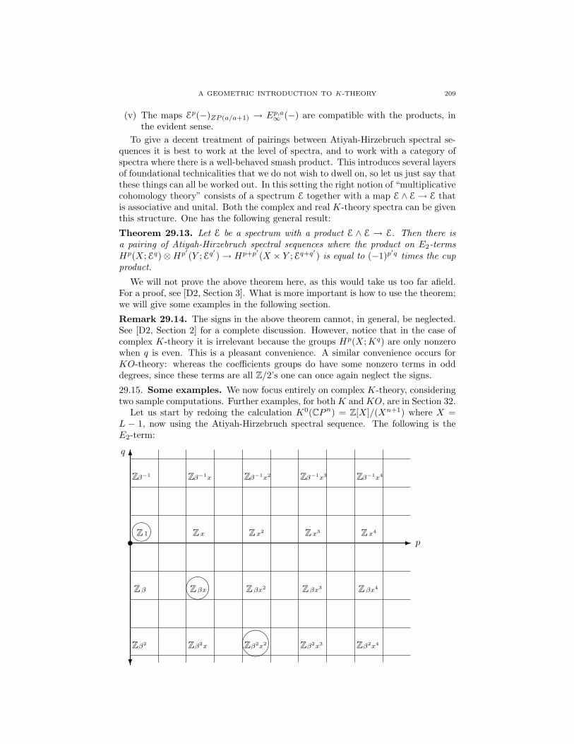
A GEOMETRIC INTRODUCTION TO K-THEORY 209
(v) The maps Ep(−)ZP (a/a+1) → Ep,a∞ (−) are compatible with the products, inthe evident sense.
To give a decent treatment of pairings between Atiyah-Hirzebruch spectral se-quences it is best to work at the level of spectra, and to work with a category ofspectra where there is a well-behaved smash product. This introduces several layersof foundational technicalities that we do not wish to dwell on, so let us just say thatthese things can all be worked out. In this setting the right notion of “multiplicativecohomology theory” consists of a spectrum E together with a map E ∧ E→ E thatis associative and unital. Both the complex and real K-theory spectra can be giventhis structure. One has the following general result:
Theorem 29.13. Let E be a spectrum with a product E ∧ E → E. Then there isa pairing of Atiyah-Hirzebruch spectral sequences where the product on E2-termsHp(X;Eq)⊗Hp′(Y ;Eq
′)→ Hp+p′(X × Y ;Eq+q
′) is equal to (−1)p
′q times the cupproduct.
We will not prove the above theorem here, as this would take us too far afield.For a proof, see [D2, Section 3]. What is more important is how to use the theorem;we will give some examples in the following section.
Remark 29.14. The signs in the above theorem cannot, in general, be neglected.See [D2, Section 2] for a complete discussion. However, notice that in the case ofcomplex K-theory it is irrelevant because the groups Hp(X;Kq) are only nonzerowhen q is even. This is a pleasant convenience. A similar convenience occurs forKO-theory: whereas the coefficients groups do have some nonzero terms in odddegrees, since these terms are all Z/2’s one can once again neglect the signs.
29.15. Some examples. We now focus entirely on complex K-theory, consideringtwo sample computations. Further examples, for bothK andKO, are in Section 32.
Let us start by redoing the calculation K0(CPn) = Z[X]/(Xn+1) where X =L − 1, now using the Atiyah-Hirzebruch spectral sequence. The following is theE2-term:
Z Z Z Z Z1 x x2 x3 x4
Z Z Z Z Zβ−1 β−1x β−1x2 β−1x3 β−1x4
Z Z Z Z Zβ βx βx2 βx3 βx4
Z Z Z Z Zβ2 β2x β2x2 β2x3 β2x4
t -
6
?
p
q

210 DANIEL DUGGER
Note that the E2-term vanishes to the right of the line p = 2n, since H∗(CPn)vanishes in this range. The circled groups (and others along the same diagonal)are the ones that contribute to K0(CPn). Note that there is no room for anydifferentials, because the nonzero groups only occur when both p and q are even.So the spectral sequence immediately collapses, and E2 = E∞. It follows that thefiltration quotients for the ZP -filtration on K0(CPn) are as follows:
K0(CPn) K0(CPn)ZP1ooZoo K0(CPn)ZP2
oo0oo K0(CPn)ZP3ooZoo · · ·oooo
with the Z’s appearing exactly n + 1 times. Since the quotients are free there areno extension problems and we conclude that K0(CPn) ∼= Zn+1 as abelian groups.
The spectral sequence also gives information about the ring structure onK0(CPn). Note that K0(CPn)ZP1 = K0(CPn), and that K0(CPn)ZP2 =K0(CPn)ZP1 by the previous paragraph. Consider the canonical map
K0(CPn)ZP (2/3)
∼=−→ E2,−2∞ = Z〈βx〉.
Let α denote a preimage for βx under this isomorphism. The multiplicativity ofthe spectral sequence tells us that αk maps to βkxk under the corresponding mapK0(CPn)ZP (2k/2k+1) → E2k,−2k
∞ . In particular, αk is nonzero for k < n + 1. Weknow αn+1 = 0, either by Lemma 20.2 or by the fact that αn+1 ∈ K0(CPn)ZP (2n+2)
and this filtration group is zero by the spectral sequence.Now consider the map Z[α]/(αn+1) → K0(CPn). This may be regarded as a
map of filtered rings, where the domain is filtered by the powers of (α) and thetarget has the ZP -filtration. The spectral sequence tells us this is an isomorphismon the filtration quotients; but since there are only finitely many of these, it followsthat the map is an isomorphism.
To complete our calculation is only remains to show that we may take α =±(1− [L]). First verify this when n = 1, where it just comes down to the fact that1 − [L] is a generator for K0(S2). For general n we can now use the naturalityof the spectral sequence, applied to the inclusion j : CP 1 → CPn. The spectralsequences tell us that the natural map
K0(CPn)ZP (2/3) → K0(CP 1)ZP (2/3)
is an isomorphism. The element 1− [L] represents an element in the domain, whichmust be a generator precisely because it maps to a generator in the target. Thistells us that one of ±(1 − [L]) maps to βx and is therefore a candidate for α, andthis is enough to conclude K0(CPn) = Z[X]/(Xn+1) where X = 1− [L].
For our next example let us consider K0(RPn). The E2-term is very similar tothe one before, with the difference that most Z’s are changed to Z/2’s:

A GEOMETRIC INTRODUCTION TO K-THEORY 211
Z2 Z2 Z2 Z2
1
β−1
β
β2
Z
Z
Z
Z2 Z2 Z2 Z2y y2 y3 y4
Z2 Z2 Z2 Z2
Z Z2 Z2 Z2 Z2
t -
6
?
p
q
· · ·
· · ·
· · ·
· · ·
Z2ym
Z2
Z2
Z2
(Z)
(Z)
(Z)
(Z)
The Z’s in parentheses lie in degree p = n when n is odd, and are not presentwhen n is even. As discussed in (29.7) above, there can be no differential emanatingfrom the p = 0 column. So the only possible differentials allowed by the gradingwould occur when n is odd and would have a Z/2 mapping into one of the Z’s; butsuch a map must be zero. So all differentials vanish, and we again have E2 = E∞.We conclude that the associated graded of the ZP -filtration on K0(RPn) consists ofbn2 c copies of Z/2, and so K0(RPn) is an abelian group of order 2b
n2 c. It remains to
determine the group precisely. For this, use the map of spectral sequences inducedby j : RPn → CPn. The surjection on E∞-terms shows that α = 1−[j∗L] generatesthe filtration quotient K0(RPn)ZP (2/3), since 1 − [L] generates the correspondingquotient in the CPn case. Note that α2, . . . , αb
n2 c therefore generate the other
filtration quotients, and so in particular are nonzero. But we can compute
α2 = (1− [j∗L])2 = 1− 2[j∗L] + [j∗L]2 = 1− 2[j∗L] + 1 = 2(1− [j∗L]) = 2α,
where in the third equality we have used that the square of any real line bundleis trivial (Corollary 8.23). It follows that αi = 2i−1α. Since αb
n2 c 6= 0 this gives
2(bn2 c−1)α 6= 0. The only abelian group of order 2b
n2 c that admits such an element
is Z/(2bn2 c), and so K0(RPn) is isomorphic to this cyclic group.
Remark 29.16. Note that we previously determined that K0(RP 2) was an abeliangroup of order 4, back in Section 13.10. Comparing the “brute force” approach usedthere to the spectral sequence machinery really shows the power of the latter: theargument is really the same, but the spectral sequence allows us to get at theconclusion much more quickly.
29.17. More on differentials. Since Kodd(pt) = 0 it follows for degree rea-sons that all differentials d2r vanish in the Atiyah-Hirzebruch spectral sequence.So our first significant differential is d3, which is a stable cohomology operationH∗(−; Z) → H∗+3(−; Z). It is an easy matter to compute all such stable opera-tions, as they are parameterized by the group H3(HZ) of stable homotopy classesHZ → Σ3HZ; this can be computed as the cohomology group Hn+3(K(Z, n)) forn ≥ 3. A routine calculation (say, with the Serre spectral sequence) shows that this
212 DANIEL DUGGER
group is Z/2. The nonzero element is an operation α that is an integral lift of Sq3,in the sense that if u ∈ H∗(X; Z) then
α(u) = Sq3(u)
where x denotes the mod 2 reduction of a class x.The above paragraph shows that our differential d3 either equals zero (for all
spaces X) or coincides with the operation α. The latter option is the correct one,and to see this it suffices to produce a single space X where d3 is nonzero. Forthis we take the space X from Example 24.7, constructed as the cofiber of a mapΣ3RP 2 → S3 that gives a null-homotopy for 2η. This space has H3(X) = Z andH6(X) = Z/2, so there is a potential d3 in the spectral sequence. If this d3 werezero then we would have K0(X) = Z/2, but we calculated in Example 24.7 (usingthe Chern character) that K0(X) = 0. So d3 is nonzero here. We have thereforeproven:
Proposition 29.18. The differential d3 in the Atiyah-Hirzebruch spectral sequenceis the unique nonzero cohomology operation H∗(−; Z) → H∗+3(−; Z). It satisfies2d3(x) = 0, for all x.
Remark 29.19. We have now explained the motivation for the space X fromExample 24.7. It is literally the smallest space for which there is a nonzero α-operation in its cohomology.
The fact that 2d3(x) = 0 shows that d3 must vanish on any class x ∈ H∗(X)whose order is prime to 2. Alternatively, if we tensor the Atiyah-Hirzebruch spec-tral sequence with Z[ 12 ] then all d3 differentials vanish. In that case d5 is a coho-mology operation H∗(−; Z[ 12 ]) → H∗+5(−; Z[ 12 ]), and such things are classfied byH5(HZ; Z[ 12 ]). This group is readily calculated to be Z/3. If one then also inverts3 this will kill d5, but it turns out to also kill d7 because H7(HZ; Z[ 16 ]) = 0. Thed9 differential becomes a cohomology operation in H9(HZ; Z[ 16 ]) ∼= Z/5, and soone can kill it by inverting 5. This process continues, and shows that invertingall primes smaller than p kills all differentials below d2p−1. Note that this givesanother proof of Proposition 29.8 (but with more precise information), saying thatafter tensoring with Q all Atiyah-Hirzebruch differentials vanish.
The following result summarizes and expands the discussion in the last para-graph. The two parts are closely related and almost equivalent, but it is useful tohave them both stated explicitly.
Proposition 29.20. Fix a prime p.(a) Inverting (p − 1)! in the Atiyah-Hirzebruch spectral sequence results in dr = 0
for r < 2p−1, together with d2p−1(u) = (−1)p+1βP 1(u) for all classes u, whereu is reduction modulo p, P 1 is Steenrod’s first reduced power operation (for theprime p), and β is the Bockstein for the sequence 0→ Z[ 1
(p−1)! ]p−→ Z[ 1
(p−1)! ]→Z/p→ 0.
(b) Let u ∈ H∗(X) be pe-torsion, where p is a prime. Then in the Atiyah-Hirzebruch spectral sequence di(u) = 0 for i < 2p − 1, and d2p−1(u) =(−1)p+1βP 1(u) where β is the Bockstein for 0→ Z p−→ Z→ Z/p→ 0 and P 1
is as in (a).
Proof. Fixing a prime p, the following is known about H∗(K(Z, n)) assuming n >2p− 1:
A GEOMETRIC INTRODUCTION TO K-THEORY 213
(i) Hi(K(Z, n)) = 0 for 0 < i < n and Hn(K(Z, n)) ∼= Z;(ii) Hi(K(Z, n)) is torsion, with all orders prime to p, for n < i < n+ 2p− 1;(iii) Hn+2p−1(K(Z, n)) is isomorphic to a direct sum Z/p⊕A where A is a torsion
group whose order only has prime factors smaller than p. The Z/p summandis generated by βP 1(u), where u ∈ Hn(K(Z, n)) is the fundamental class.
Alternatively, the above results say that
H∗(K(Z, n); Z[ 1
(p−1)! ])∼=
0 if i < n,
Z[ 1(p−1)! ] if i = n,
0 if n < i < n+ 2p− 1,Z/p if i = n+ 2p− 1.
These facts are easy calculations with the Serre spectral sequence, using the meth-ods of [MT, Chapter ???].
Consider the Atiyah-Hirzebruch spectral sequence for K(Z, n), and in particularthe differentials on the fundamental class u. By naturality of the spectral sequencethis serves as a universal example for what happens on all spaces. Since inverting(p− 1)! kills all of the cohomology of K(Z, n) in dimensions strictly between n andn + 2p − 1, this shows that it also kills the differentials dr(u) for r < 2p − 1. Byuniversality, inverting (p− 1)! kills these differentials for any space X.
If u ∈ H∗(X) is a pe-torsion class then dr(u) for r < 2p−1 is killed by a power of(p− 1)! by the preceding paragraph, but it is also killed by pe; since these integersare relatively prime it follows that dr(u) = 0 for r < 2p− 1.
It remains to identify d2p−1 in both (a) and (b). We know by the calculation ofH∗(K(Z, n)) for n 0 that after localization at (p− 1)! one must have d2p−1(u) =λ ·βP 1(u), for some λ ∈ Z/p. We need to determine λ, and for this we can examinea single well-chosen example space. The sample space we choose is a generalizationof the one from Example 24.7. Consider the projection π : CP p → CP p/CP p−1 ∼=S2p. We claim that there is a stable map f : S2p → CP p such that the compositeS2p → CP p π−→ S2p has degreeMp for some integerM prime to p; for the proof, seeLemma 29.22 below. The “stable map” phrase is to indicate that f might only existafter suspensing some number of times, so really it is a map f : ΣrS2p → ΣrCP p.We can assume that r is even. Let X be the cofiber of f , and note that
Hi(X) =
Z if r + 2 ≤ i < r + 2p and i is even,Z/(Mp) if i = r + 2p+ 1,0 otherwise.
Consider the cofiber sequence
ΣrCP p j−→ Xp−→ Sr+2p+1
Let x ∈ H2(CP p) be a chosen generator, and let u ∈ Hr+2(X) be a class that j∗
maps onto the suspension σr(x). Let v ∈ Hr+2p+1(X) be the image under p∗ ofthe canonical generator from Hr+2p+1(Sr+2p+1). Note that j∗ is an isomorphismon H∗(−; Z/p) for ∗ ≤ 2p.
In H∗(CP p; Z/p) we have P 1(x) = xp, as this is how P 1 behaves on classes ofdegree 2. So in H∗(ΣrCP p; Z/p) we have P 1(σrx) = σr(xp), by stability of the P 1
operation. It follows that βP 1(u) = Mv.
214 DANIEL DUGGER
In the Atiyah-Hirzebruch spectral sequence for X, after inverting (p− 1)! thereis only one possible nonvanishing differential, namely d2p−1 : Z[ 1
(p−1)! ] → Z/p. Weknow that
d2p−1(u) = λ · βP 1(u) = λMv.(29.21)
But we can also compute d2p−1(u) directly. The class u is represented by an ele-ment in K0(Xr+2, Xr+1) (a cellular (r+2)-cochain). The differential is representedby choosing a lift of u ∈ K0(Xr+2, Xr+1) to ξ ∈ K0(X2p+r, Xr+1) and then ap-plying the connecting homomorphism from the long exact sequence for the triple(X2p+r+1, X2p+r, Xr+1):
ξ ∈ K0(X2p+r+1, Xr+1)
δ // K1(X2p+r+1, X2p+r)
u ∈ K0(Xr+2, Xr+1).
Recall that Xr+1 = ∗ and that u is represented by the class σr(1 − [L]) ∈K0(ΣrCP 1). The element 1− [L] ∈ K0(CP 1) lifts to the class with the same namein K0(CP p), and so we may take ξ = σr(1 − [L]) ∈ K0(ΣrCP p, ∗). To computeδ(ξ) we can use the Chern character:
K0(X2p+r, ∗)δ //
ch
K1(X2p+r+1, X2p+1)
ch
Hev(X2p+r, ∗; Q) δ // Hodd(X2p+r+1, X2p+1; Q).
We know from Proposition 24.4 that the right vertical map is an injection and thatits image is the integral subgroup Hodd(X2p+r+1, X2p+1; Z). So we compute
ch(ξ) = ch(σr(1− [L])
)= σr ch(1− [L]) = σr(x− x2
2 + x3
6 − · · · )Applying δ to this expresstion kills everything except the class in degree 2p + r,and we therefore get
δ(ch ξ) = (−1)p · 1p! ·Mp = (−1)p M
(p−1)!
where the first two terms in the product come from ch(ξ) and the Mp comes fromapplication of δ. Note that commutativity of the above square implies that M
(p−1)!
must be an integer, and that
δ(ξ) = (−1)p M(p−1)! · v
where v denotes the preferred generator of K1(X2p+r+1, X2p+r) ∼= Z.Putting everything together, we have just proven that in the Atiyah-Hirzebruch
spectral sequence for X with (p− 1)! inverted one has
d2p−1(u) =[(−1)p M
(p−1)!
]p· v
where [−]p denotes the residue modulo p. Wilson’s Theorem says that (p−1)! ≡ −1mod p, and so
d2p−1(u) =[(−1)p+1M
]p· v.
Comparing to (29.21) gives λ = (−1)p+1, and we are finished with (a).
A GEOMETRIC INTRODUCTION TO K-THEORY 215
Part (b) can be deduced from (a) using the commutative square
H∗(X)d2p−1 //
H∗+2p−1(X)
H∗(X; Zf )
d2p−1 // H∗+2p−1(X; Zf )
where we are writing Zf = Z[ 1(p−1)! ]. Let B ⊆ H∗+2p−1(X) be the subgroup of
elements killed by a power of p, and note that B injects into H∗+2p−1(X; Zf ). Ifpeu = 0 then both d2p−1u and (−1)p+1βP 1(u) belong to B. The commutativesquare, together with part (a), show that the two classes map to the same elementof H∗+2p−1(X; Zf ); hence, they are the same.
Lemma 29.22. Fix a prime p. Then for some r > 0 there exists a map S2p+r →ΣrCP p such that the composite
S2p+r → ΣrCP p Σrπ−→ ΣrS2p
has degree equal to Mp for some M relatively prime to p. Here π : CP p → S2p isthe map that collapses CP p−1 to a point.
Proof. This is a computation with stable homotopy groups. Consider the homologytheory X 7→ E∗(X) = πs∗(X) ⊗ Z(p). When X = S0 the groups E∗(X) are the p-components of the stable homotopy groups of spheres, and it is known that Ei(X) =0 for 0 < i < 2p − 3 and E2p−3(X) ∼= Z/p. An easy induction using the cofibersequences CPn−1 → CPn → S2n shows that E2p−1(CPn) ∼= Z/p for all 1 ≤ n ≤p− 1. The long exact sequence for CP p−1 → CP p → S2p then gives
· · · → πs2p(CPp−1)→ πs2p(CP
p)→ Z→ πs2p−1(CPp−1)→ · · ·
The element p ∈ Z necessarily maps to zero in πs2p−1(CPp−1)⊗Z(p), since the latter
group is Z/p. This means that there exists M ∈ Z prime to p such that Mp mapsto zero in πs2p−1(CP
p−1). But then Mp is the image of an element in πs2p(CPp),
and this element is what we were looking for.
29.23. Differentials and the Chern character. In the proof of Proposi-tion 29.20 there was a key step where we used the Chern character to help computea differential in the Atiyah-Hirzebruch spectral sequence. We will next explain ageneralization of this technique.
The E1-term of the Atiyah-Hirzebruch spectral sequence breaks up into chaincomplexes that look like
· · · → K−1(Fq−1, Fq−2)→ K0(Fq, Fq−1)→ K1(Fq+1, Fq)→ · · ·If q is odd this is the zero complex, and if q is even we have seen that it is iso-morphic to the cellular chain complex for X with Z coefficients. The latter isvia isomorphisms K0(Fq, Fq−1) ∼= K0(∨αSq) ∼=
⊕α K
0(Sq) ∼=⊕
α Z. Noticethat we can also use the Chern character to obtain such an isomorphism, as weknow ch: K0(Fq, Fq−1) → H∗(Fq, Fq−1; Q) to be injective with image equal to

216 DANIEL DUGGER
H∗(Fq, Fq−1; Z) (Proposition 24.4). Since the Chern character is natural it actu-ally gives us an isomorphism of chain complexes
· · · // K−1(Fq−1, Fq−2)
∼=
// K0(Fq, Fq−1) //
∼=
K1(Fq+1, Fq) //
∼=
· · ·
· · · // H∗(Fq−1, Fq−2) // H∗(Fq, Fq−1) // H∗(Fq+1, Fq) // · · ·
Taken on its own, this is just a matter of convenience: we already had a naturalisomorphism between these complexes, so identifying it as the Chern characterjust gives it a nice name. But using the fact that the Chern character is definedmore globally (i.e., on all pairs (Y,B)) allows us to push this a bit further andobtain a description of the Atiyah-Hirzebruch differentials. The following result isa combination of [AH2, Lemmas 1.2 and 7.3]
Proposition 29.24. Let X be a CW -complex and let u ∈ Hp(X). Then in theAtiyah-Hirzebruch spectral sequence one has diu = 0 for all 2 ≤ i < r if and onlyif there exist u ∈ Hp(Fp+r−1, Fp−1) and ξ ∈ K∗(Fp+r−1, Fp−1) such that
(i) u is a lift for u under Hp(Fp+r−1, Fp−1)→ Hp(Fp+r−1)∼=←− Hp(X), and
(ii) ch(ξ) = u+ higher order terms.Moreover, if in the above situation α is a cellular cochain representating ch(ξ)p+r−1
then δα is integral and represents the differential dru.
Proof. To symplify some typography we assume throughout the proof that p iseven, although the odd case is identical (or else one could just replace X with itssuspension).
Assume that u ∈ Hp(X) satisfies diu = 0 for 2 ≤ i < r. Identifying u with anelement in E2, this condition says that u can be represented by a class z ∈ E1 =K0(Fp, Fp−1) with the property that z ∈ Zr−1. The element associated to z by theisomorphism K0(Fp, Fp−1) ∼= Cpcell(X; Z) is a cellular p-cochain representative foru.
As remarked in (8) of Section 29.1, the condition z ∈ Zr−1 is equivalent to sayingthat z lifts to a class z ∈ K0(Fp+r−1, Fp−1). Now apply the Chern character to getthe square
K0(Fp+r−1, Fp−1) //
ch
K0(Fp, Fp−1)
ch
H∗(Fp+r−1, Fp−1; Q)
j∗ // H∗(Fp, Fp−1; Q),
z //
z
ch(z) // ch(z).
The element ch(z) is an (integral) cellular p-cochain that represents the class u.The groups H∗(Fp+r−1, Fp−1) are zero in degrees ∗ < p, so ch(z) is of the formch(z)p + higher order terms. The fact that ch(z) is a cellular cochain representingu says that any lift of ch(z) into Hp(Fp+1, Fp−1) has the same image in Hp(Fp+1)as u:
Hp(X) // Hp(Fp+1) Hp(Fp+1, Fp−1)oo
It follows readily that ch(z)p has the same image in Hp(Fp+r−1) as u. This com-pletes the (⇒) direction of the first statement in the proposition. The (⇐) directionfollows in the same way, as all the steps are reversible.
A GEOMETRIC INTRODUCTION TO K-THEORY 217
For the final statement of the proposition we continue to assume (for convenience)that p is even. Consider the diagram
ξ ∈ K0(Fp+r−1, Fp−1)
ch
δ // K1(Fp+r, Fp+r−1)
ch
H∗(Fp+r−1, Fp−1; Q) δ // H∗+1(Fp+r, Fp+r−1; Q)
where in both rows the map δ is the connecting homomorphism in the long exactsequence for the triple (Fp+r, Fp+r−1, Fp−1). Looking back on (8) of Section 29.1,the element δ(ξ) represents dr(u) in the Er-term of the spectral sequence. But weknow that the right vertical map is an injection whose image consists of the integralelements, and our isomorphism of the E2-term with H∗(X; Z) identifies δ(ξ) withch(δ(ξ)). Commutativity of the square says this element is also δ((ch ξ)q+r−1) (andalso verifies that this class is integral).
30. Operations on K-theory
Experience has shown that when studying a cohomology theory it is useful tolook not just at the cohomology groups themselves but also the natural operationson the cohomology groups. In the case of singular cohomology this is the theory ofSteenrod operations. In the present section we will construct some useful operationsK0(X) → K0(X). We start with the λ-operations, which are easy to define buthave the drawback that they are not group homomorphisms. Then we modify theseto obtain the Adams operations ψk, which are more nicely behaved.
30.1. The lambda operations. Fix a topological space X. We start with theexterior power constructions E 7→ ΛkE on vector bundles over X. These are, ofcourse, not additive: Λk(E ⊕F ) 6∼= ΛkE ⊕ΛkF . So it is not immediately clear howthese constructions induce maps on K-groups. The key lies in the formula
Λk(E ⊕ F ) ∼=⊕i+j=k
ΛiE ⊗ ΛjF.(30.2)
Construct a formal power series
λt(E) =∞∑i=0
[ΛiE]ti = 1 + [E]t+ [Λ2E]t2 + · · · ∈ K0(X)[[t]].
Because the zero coefficient is 1, this power series is a unit in K0(X)[[t]]. So λt isa function into the group of units inside K0(X)[[t]]:
Vect(X)λt //
(K0(X)[[t]]
)∗
K0(X)
88
Formula (30.2) says that λt(E ⊕ F ) = λt(E) · λt(F ), and this implies the existenceof the dotted-arrow group homomorphism in the above diagram. We will call thisdotted arrow λt as well.

218 DANIEL DUGGER
Finally, define λk : K0(X)→ K0(X) by letting λk(w) be the coefficient of tk inλt(w). Note that if E is a vector bundle over X then λk([E]) = [ΛkE]. However,λk is not a group homomorphism; instead one has the formula
λk(u+ w) =∑i+j=k
λi(u)λj(v).
Example 30.3. To get a feeling for these operations let us compute λk(−[E]) forE a vector bundle over X. Note first that
λt(−[E]) = 1λt([E]) = 1
1+[E]t+[Λ2E]t2+···
For R a commutative ring and a = 1 + a1t+ a2t2 + · · · ∈ R[[t]], one has
1a = 1 + P1t+ P2t
2 + · · ·where the Pi’s are certain universal polynomials in the ai’s with coefficients in Z.Equating coefficients in the identity 1 = (1+ a1t+ a2t
2 + · · · )(1+P1t+P2t2 + · · · )
givesPk + Pk−1a1 + Pk−2a2 + · · ·+ P1ak−1 + ak = 0,
which allows one to inductively determine each Pk. One finds that
P1 = −a1, P2 = a21 − a2, P3 = −a3
1 − 2a1a2 + a3
So we conclude that
λ1(−[E]) = −[E],
λ2(−[E]) = [E]2 − [Λ2E],
λ3(−[E]) = −[E]3 − 2[E][Λ2E] + [Λ3E]
and so forth.
30.4. Symmetric power operations. One can repeat everything from the pre-vious section using the symmetric product construction E 7→ Symk E in place ofthe exterior product ΛkE. One obtains a group homomorphism
symt : K0(X)→
(K0(X)[[t]]
)∗and defines symk(w) to be the coefficient of tk in symt(w). It turns out, how-ever, that these operations do not give anything ‘new’—they are related to theλ-operations by the formula
symk(w) = λk(−w).
To explain this we need a brief detour on the deRham complex. The followingmaterial is taken from [FLS].
Let V be a vector space over a field F . Write Sym∗(V ) = ⊕k Symk(V ) andΛ∗(V ) = ⊕kΛkV . These each have a familiar algebra structure, and we havecanonical isomorphisms
Sym∗(V )⊗ Sym∗(W )∼=−→ Sym∗(V ⊕W ), Λ∗(V )⊗ Λ∗(W )
∼=−→ Λ∗(V ⊕W ).
These isomorphisms allow us to equip both Sym∗(V ) and Λ∗(V ) with coproductsmaking them into Hopf algebras. The coproducts are
Sym∗(V ) −→ Sym∗(V ⊕ V )∼=←− Sym∗(V )⊗ Sym∗(V )
andΛ∗(V ) −→ Λ∗(V ⊕ V )
∼=←− Λ∗(V )⊗ Λ∗(V )
A GEOMETRIC INTRODUCTION TO K-THEORY 219
where in each case the first map is the one induced by the diagonal ∆: V → V ⊕V .Write e : Symk(V )→ Symk−1 V ⊗ Sym1(V ) and e′ : Λk(V )→ Λ1V ⊗ Λk−1(V ) forthe projections of the coproduct onto the indicated factors. Finally, write d and κfor the composites
Symk(V )⊗ Λi(V )e⊗id// Symk−1(V )⊗ Sym1(V )⊗ Λi(V )
Symk−1(V )⊗ Λ1(V )⊗ Λi(V ) // Symk−1(V )⊗ Λi+1(V )
and
Symk(V )⊗ Λi(V )id⊗e′// Symk(V )⊗ Λ1(V )⊗ Λi−1(V )
Symk(V )⊗ Sym1(V )⊗ Λi−1(V ) // Symk+1(V )⊗ Λi−1(V ).
The maps d and κ are called the de Rham and Koszul differentials, respectively.The following diagram shows the maps d, and the maps κ go in the opposite direc-tion:
The deRham and Koszul complexes:(30.5)
......
......
Sym3 V ⊗ Λ2V
d
66llllllllllllllSym2 V ⊗ Λ2V
d
66llllllllllllllSym1 V ⊗ Λ2V
d
66llllllllllllllSym0 V ⊗ Λ2V
Sym3 V ⊗ Λ1V
d
66mmmmmmmmmmmmSym2 V ⊗ Λ1V
d
66mmmmmmmmmmmmSym1 V ⊗ Λ1V
d
66mmmmmmmmmmmmSym0 V ⊗ Λ1V
Sym3 V ⊗ Λ0V
d
66mmmmmmmmmmmmSym2 V ⊗ Λ0V
d
66mmmmmmmmmmmmSym1 V ⊗ Λ0V
d
66mmmmmmmmmmmmSym0 V ⊗ Λ0V
Let e1, . . . , en be a basis for V . It will be convenient to use the notation dejfor the element of Λ1(V ) corresponding to ej under the canonical isomorphismΛ1(V ) ∼= V . Let m = ei1 ⊗ · · · ⊗ eir ∈ Symr(V ) and ω = dej1 ∧ · · · ∧ dejs ∈ Λs(V ).It is an exercise to verify that
e(m) =∑u
(ei1 ⊗ · · · ⊗ eiu ⊗ · · · ⊗ eir
)⊗ eiu
ande′(ω) =
∑u
(−1)u−1deju ⊗(dej1 ∧ · · · ∧ deju ∧ · · · ∧ dejs
).
Sod(m⊗ ω) =
∑u
(ei1 ⊗ · · · ⊗ eiu ⊗ · · · ⊗ eir
)⊗ (deiu ∧ ω)
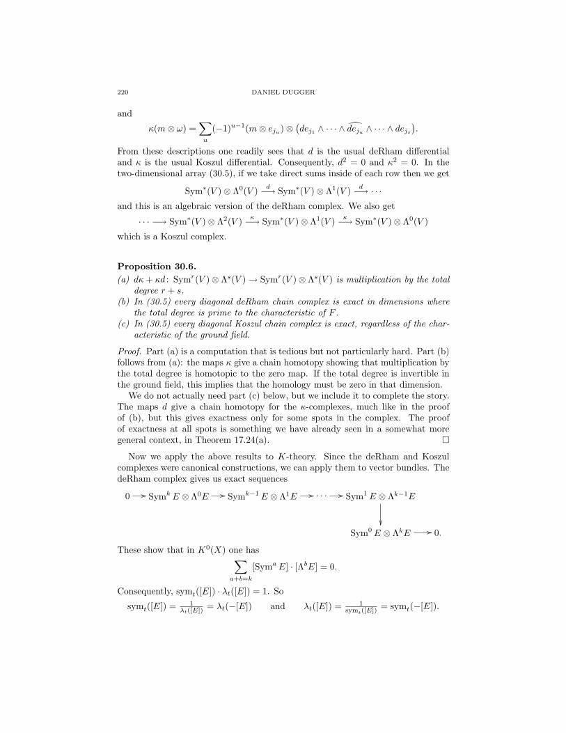
220 DANIEL DUGGER
and
κ(m⊗ ω) =∑u
(−1)u−1(m⊗ eju)⊗(dej1 ∧ · · · ∧ deju ∧ · · · ∧ dejs
).
From these descriptions one readily sees that d is the usual deRham differentialand κ is the usual Koszul differential. Consequently, d2 = 0 and κ2 = 0. In thetwo-dimensional array (30.5), if we take direct sums inside of each row then we get
Sym∗(V )⊗ Λ0(V ) d−→ Sym∗(V )⊗ Λ1(V ) d−→ · · ·and this is an algebraic version of the deRham complex. We also get
· · · −→ Sym∗(V )⊗ Λ2(V ) κ−→ Sym∗(V )⊗ Λ1(V ) κ−→ Sym∗(V )⊗ Λ0(V )
which is a Koszul complex.
Proposition 30.6.(a) dκ+ κd : Symr(V )⊗ Λs(V )→ Symr(V )⊗ Λs(V ) is multiplication by the total
degree r + s.(b) In (30.5) every diagonal deRham chain complex is exact in dimensions where
the total degree is prime to the characteristic of F .(c) In (30.5) every diagonal Koszul chain complex is exact, regardless of the char-
acteristic of the ground field.
Proof. Part (a) is a computation that is tedious but not particularly hard. Part (b)follows from (a): the maps κ give a chain homotopy showing that multiplication bythe total degree is homotopic to the zero map. If the total degree is invertible inthe ground field, this implies that the homology must be zero in that dimension.
We do not actually need part (c) below, but we include it to complete the story.The maps d give a chain homotopy for the κ-complexes, much like in the proofof (b), but this gives exactness only for some spots in the complex. The proofof exactness at all spots is something we have already seen in a somewhat moregeneral context, in Theorem 17.24(a).
Now we apply the above results to K-theory. Since the deRham and Koszulcomplexes were canonical constructions, we can apply them to vector bundles. ThedeRham complex gives us exact sequences
0 // Symk E ⊗ Λ0E // Symk−1E ⊗ Λ1E // · · · // Sym1E ⊗ Λk−1E
Sym0E ⊗ ΛkE // 0.
These show that in K0(X) one has∑a+b=k
[SymaE] · [ΛbE] = 0.
Consequently, symt([E]) · λt([E]) = 1. So
symt([E]) = 1λt([E]) = λt(−[E]) and λt([E]) = 1
symt([E]) = symt(−[E]).
A GEOMETRIC INTRODUCTION TO K-THEORY 221
Any class w ∈ K0(X) has the form w = [E] − [F ] for some vector bundles E andF , and therefore
symt(w) = symt([E]) · symt(−[F ]) = λt(−[E]) · λt([F ]) = λt([F ]− [E]) = λt(−w).
So the symk and λk operations on K-theory are essentially the same: symk(w) =λk(−w).
This has been a long discussion with somewhat of a negative conclusion: thesymk operations can be completely ignored in favor of the λk’s (or vice versa). Wehave learned some useful things along the way, however.
30.7. The Newton polynomials. The usefulness of the λk operations is limitedby the fact that they are not group homomorphisms. There is a clever method,however, for combining the λ-operations in a way that does produce a collectionof group homomorphisms. This is originally due to Frank Adams [Ad2]. Beforedescribing this construction we take a brief detour to develop the algebraic combi-natorics that we will need.
Moved to appendix
30.8. The Adams operations. Recall that we have a map λt : K0(X) →(K0(X)[[t]]
)∗ and that this is a group homomorphism:
λt(x+ y) = λt(x) · λt(y).If we want additive maps K0(X) → K0(X) a natural idea is to apply logarithmsto the above formula. To be precise, start with the formal power series
log(1 + z) = z − z2
2 + z3
3 − · · ·Since λt(x) has constant term equal to 1, we can use the above series to make senseof log(λt(x))—but only provided that we add denominators into K0(X), say bytensoring with Q. If we set µt(x) = log(λt(x)) then we would have
µt(x+ y) = µt(x) + µt(y).
The coefficients of powers of t in µt(x) then give additive operations, with the onlydifficulty being that they take values in K0(X)⊗Q.
We can, however, eliminate the need for Q-coefficients by applying the operatorddt . Precisely, define
νt(x) =d
dt
[µt(x)
]= λ′t(x)
λt(x)= (1− z + z2 − z3 + · · · )|z=λt(x)−1 · λ′t(x).
Clearly this eliminates the problem with denominators: νt(x) ∈ K0(X)[[t]], yetwe still have νt(x + y) = νt(x) + νt(y). Taking coefficients of νt(x) thereby yieldsadditive operations νk : K0(X)→ K0(X).
We could stop here, but there is one more modification that makes things a bitsimpler later on. Suppose that L is a line bundle over X, and take x = [L]. Thenλt(x) = 1 + [L]t = 1 + xt, hence
νt(x) = x1+xt = x(1− xt+ x2t2 − x3t3 + · · · ) = x− x2t+ x3t2 − · · · .
The ν-operations simply give powers of x, together with certain signs: νk(x) =(−1)kxk−1. It is easy to adopt a convention that makes these signs disappear, andwe might as well do this; and while we’re at it, lets shift the indexing on the ν’s sothat the kth operation sends x to xk, since that will be easier to remember.

222 DANIEL DUGGER
Putting everything together, we have arrived at the following definition:
ψt(x) = td
dt
[log(λ−t(x))
]= t · λ
′−t(x)
λ−t(x),
and ψk(x) is the coefficient of tk in ψt(x). The operations ψk are called Adamsoperations. We have proven that(1) Each ψk is a group homomorphism K0(X)→ K0(X), natural in X;(2) If x = [L] for L a line bundle then ψk(x) = xk.
Conditions (1) and (2) actually completely characterize the Adams operations,although we will not need this.
The following identities give a recursive formula for the Adams operations interms of the λ-operations:
Proposition 30.9.(a) ψk = Sk(λ1, . . . , λk), where Sk is the kth Newton polynomial;(b) ψk = λ1ψk−1 − λ2ψk−1 + · · ·+ (−1)kλk−1ψ1 + (−1)k+1kλk.
Proof. Part (b) is, of course, an immediate consequence of (a) via Lemma B.1. Part(a) follows directly from Proposition B.3.
We record the first few Adams operations:
ψ1 = λ1, ψ2 = (λ1)2 − 2λ2, ψ3 = (λ1)3 − 3λ1λ2 + 3λ3.
For more of these, just see Table 2.2.
30.10. Properties of the Adams operations.
Proposition 30.11. Fix k, l ≥ 1 and x, y ∈ K0(X). Then(a) ψk(x+ y) = ψk(x) + ψk(y)(b) ψk(xy) = ψk(x)ψk(y)(c) ψk(ψl(x)) = ψkl(x)(d) If k is prime then ψk(x) ≡ xk mod k.
The proof will use the following terminology. A line element in K0(X) is anyelement [L] where L→ X is a line bundle. The span of the line elements consist ofthe classes of the form [L1] + · · ·+ [La]− [L′1]− · · · − [L′b] where the Li’s and L′j ’sare all line bundles.
Proof of Proposition 30.11. Note that if x and y are line elements then all of theabove results are obvious because ψr([L]) = [Lr]. More generally, the results followeasily if x and y are in the span of the line elements. The general result nowfollows from the splitting principle in Proposition 30.12 below. Specifically, choosea p : X1 → X such that p∗ is injective and p∗(x) is in the span of line elements.Then choose a q : X2 → X1 such that q∗ is injective and q∗(p∗(y)) is in the span ofline elements. The identities in (a)–(d) all hold for x′ = (pq)∗(x) and y′ = (pq)∗(y),and so the injectivity of (pq)∗ shows they hold for x and y as well.
Proposition 30.12 (The Splitting Principle). Let X be any space, and let x ∈K0(X). Then there exists a space Y and a map p : Y → X such that p∗ : K0(X)→K0(Y ) is injective and p∗(x) is in the span of line elements.
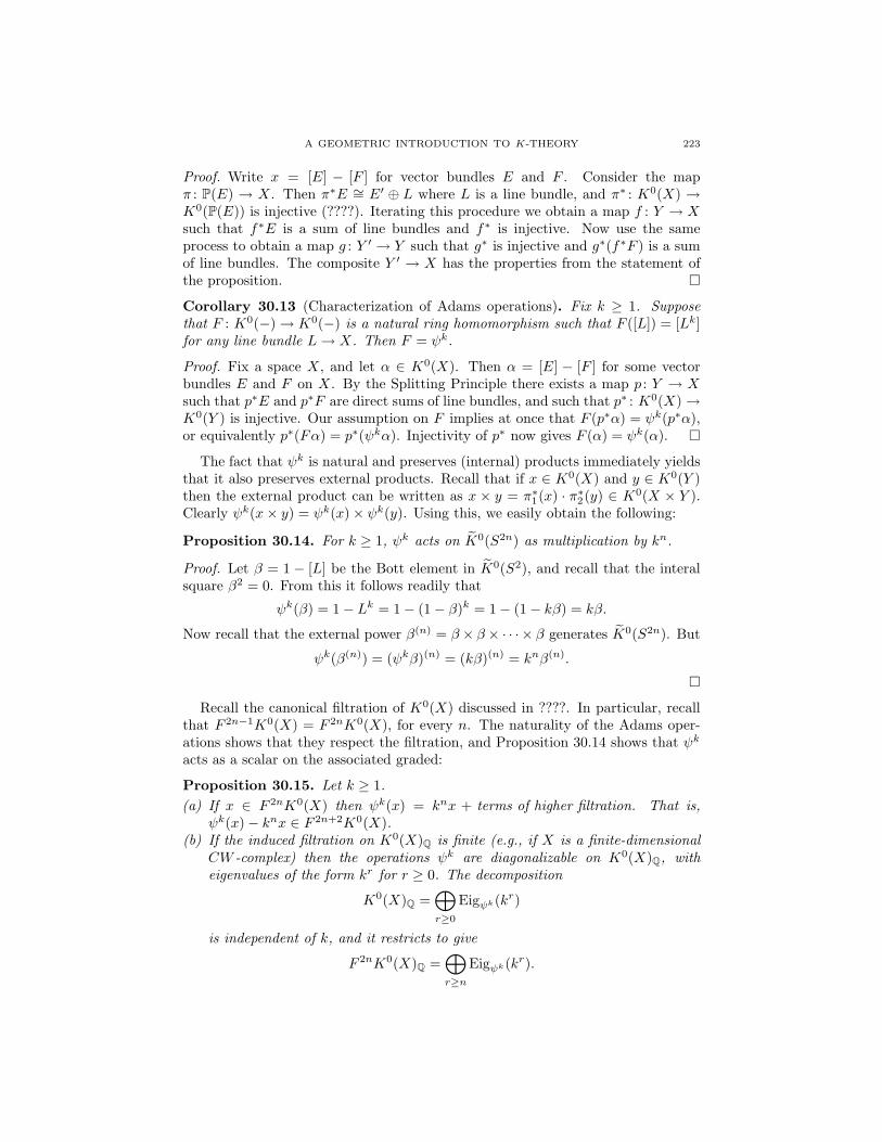
A GEOMETRIC INTRODUCTION TO K-THEORY 223
Proof. Write x = [E] − [F ] for vector bundles E and F . Consider the mapπ : P(E) → X. Then π∗E ∼= E′ ⊕ L where L is a line bundle, and π∗ : K0(X) →K0(P(E)) is injective (????). Iterating this procedure we obtain a map f : Y → Xsuch that f∗E is a sum of line bundles and f∗ is injective. Now use the sameprocess to obtain a map g : Y ′ → Y such that g∗ is injective and g∗(f∗F ) is a sumof line bundles. The composite Y ′ → X has the properties from the statement ofthe proposition.
Corollary 30.13 (Characterization of Adams operations). Fix k ≥ 1. Supposethat F : K0(−)→ K0(−) is a natural ring homomorphism such that F ([L]) = [Lk]for any line bundle L→ X. Then F = ψk.
Proof. Fix a space X, and let α ∈ K0(X). Then α = [E] − [F ] for some vectorbundles E and F on X. By the Splitting Principle there exists a map p : Y → Xsuch that p∗E and p∗F are direct sums of line bundles, and such that p∗ : K0(X)→K0(Y ) is injective. Our assumption on F implies at once that F (p∗α) = ψk(p∗α),or equivalently p∗(Fα) = p∗(ψkα). Injectivity of p∗ now gives F (α) = ψk(α).
The fact that ψk is natural and preserves (internal) products immediately yieldsthat it also preserves external products. Recall that if x ∈ K0(X) and y ∈ K0(Y )then the external product can be written as x × y = π∗1(x) · π∗2(y) ∈ K0(X × Y ).Clearly ψk(x× y) = ψk(x)× ψk(y). Using this, we easily obtain the following:
Proposition 30.14. For k ≥ 1, ψk acts on K0(S2n) as multiplication by kn.
Proof. Let β = 1 − [L] be the Bott element in K0(S2), and recall that the interalsquare β2 = 0. From this it follows readily that
ψk(β) = 1− Lk = 1− (1− β)k = 1− (1− kβ) = kβ.
Now recall that the external power β(n) = β × β × · · · × β generates K0(S2n). But
ψk(β(n)) = (ψkβ)(n) = (kβ)(n) = knβ(n).
Recall the canonical filtration of K0(X) discussed in ????. In particular, recallthat F 2n−1K0(X) = F 2nK0(X), for every n. The naturality of the Adams oper-ations shows that they respect the filtration, and Proposition 30.14 shows that ψk
acts as a scalar on the associated graded:
Proposition 30.15. Let k ≥ 1.(a) If x ∈ F 2nK0(X) then ψk(x) = knx + terms of higher filtration. That is,
ψk(x)− knx ∈ F 2n+2K0(X).(b) If the induced filtration on K0(X)Q is finite (e.g., if X is a finite-dimensional
CW -complex) then the operations ψk are diagonalizable on K0(X)Q, witheigenvalues of the form kr for r ≥ 0. The decomposition
K0(X)Q =⊕r≥0
Eigψk(kr)
is independent of k, and it restricts to give
F 2nK0(X)Q =⊕r≥n
Eigψk(kr).

224 DANIEL DUGGER
Proof. For part (a) it suffices to replace X by a weakly equivalent CW -complex,so that F 2nK0(X) = ker[K0(X) → K0(X2n−1)]. If α ∈ F 2nK0(X) then let α1
denote its image in K0(X2n). The cofiber sequence X2n−1 → X2n → X2n/X2n−1
indcues a long exact sequence
· · · → K0(X2n/X2n−1)→ K0(X2n)→ K0(X2n−1)→ · · ·The element α1 ∈ K0(X2n) maps to zero, and so it is the image of a class α2 ∈K0(X2n/X2n−1). By Proposition 30.14 one knows ψk(α2) = knα2, and so ψkα1 =knα1. It follows that ψkα − knα maps to zero in K0(X2n), and hence lies inF 2n+1K0(X2n).
For part (b), let 2n be the largest even integer such that F 2nK0(X)Q 6= 0. Itfollows from (a) that ψk acts as multiplication by kn on F 2nK0(X)Q. We nowprove by reverse induction that F 2iK0(X)Q is the sum of kj-eigenspaces of ψk, forj ≥ i. Assume this holds for a particular value of i, and let α ∈ F 2i−2K0(X). Weknow ψkα = ki−1α + γ, where γ is some element of F 2iK0(X)Q. The inductionhypothesis says that γ = σi + σi+1 + · · ·+ σn where each σr is an eigenvector witheigenvalue kr. A routine calculation now shows that α−
∑r≥i
1kr−ki−1σr is a ki−1-
eigenvector for ψk, and hence α belongs to the sum of eigenspaces for eigenvalueskr, r ≥ i− 1. This completes the induction step.
31. The Hopf invariant one problem
The Hopf invariant assigns an integer to every map f : S2n−1 → Sn, giving agroup homomorphism H : π2n−1(Sn) → Z. Elementary arguments show that 2 isalways in the image, and the natural question is then whether 1 is also in the image.This is the Hopf invariant one problem—determine all values of n for which H issurjective (or said differently, all values of n for which there exists a map of Hopfinvariant one).
It was known classically that H is surjective when n ∈ 1, 2, 4, because theclassical Hopf maps all have Hopf invariant equal to one. The question for otherdimensions was first settled by Adams in [Ad1], who proved that no other Hopfinvariant one maps exist. Adams’s proof is not simple, even by modern stan-dards, being based on secondary cohomology operations associated to the Steenrodsquares. Several years after Adams gave his original proof, Adams and Atiyahused K-theory to give a much simpler solution to the Hopf invariant one problem.Their ‘postcard proof’ takes less than a page, in dramatic contrast to Adams’soriginal method. This was seen—rightly so—as a huge demonstration of the powerof K-theory.
Our goal in this section will be to present the Adams-Atiyah proof, although wewill not quite do this in their style. Specifically, when Adams and Atiyah wrotetheir paper they clearly had an agenda: to write down the proof in as small a spaceas possible. If the goal is to accentuate how much the use of K-theory simplifies thesolution, this makes perfect sense. But at the same time, writing the proof in thisway results in a certain air of mystery: the proof involves a strange manipulationwith the Adams operations ψ2 and ψ3 that comes out of nowhere—it seems like amagic trick.
In our presentation below we try to put this (ψ2, ψ3) trick into its proper context:it is part of a calculation of a certain Ext1 group. The full calculation of this groupis not hard, and quite interesting for other reasons—e.g., it connects deeply to the
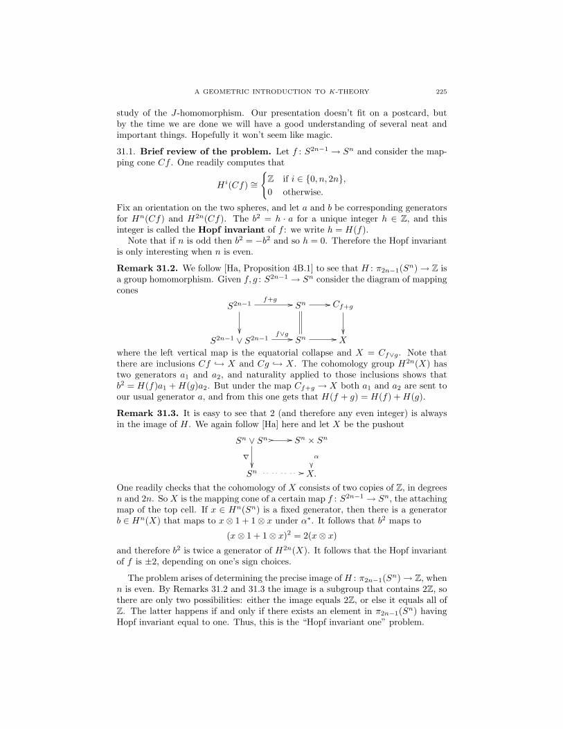
A GEOMETRIC INTRODUCTION TO K-THEORY 225
study of the J-homomorphism. Our presentation doesn’t fit on a postcard, butby the time we are done we will have a good understanding of several neat andimportant things. Hopefully it won’t seem like magic.
31.1. Brief review of the problem. Let f : S2n−1 → Sn and consider the map-ping cone Cf . One readily computes that
Hi(Cf) ∼=
Z if i ∈ 0, n, 2n,0 otherwise.
Fix an orientation on the two spheres, and let a and b be corresponding generatorsfor Hn(Cf) and H2n(Cf). The b2 = h · a for a unique integer h ∈ Z, and thisinteger is called the Hopf invariant of f : we write h = H(f).
Note that if n is odd then b2 = −b2 and so h = 0. Therefore the Hopf invariantis only interesting when n is even.
Remark 31.2. We follow [Ha, Proposition 4B.1] to see that H : π2n−1(Sn)→ Z isa group homomorphism. Given f, g : S2n−1 → Sn consider the diagram of mappingcones
S2n−1
f+g // Sn // Cf+g
S2n−1 ∨ S2n−1
f∨g // Sn // X
where the left vertical map is the equatorial collapse and X = Cf∨g. Note thatthere are inclusions Cf → X and Cg → X. The cohomology group H2n(X) hastwo generators a1 and a2, and naturality applied to those inclusions shows thatb2 = H(f)a1 +H(g)a2. But under the map Cf+g → X both a1 and a2 are sent toour usual generator a, and from this one gets that H(f + g) = H(f) +H(g).
Remark 31.3. It is easy to see that 2 (and therefore any even integer) is alwaysin the image of H. We again follow [Ha] here and let X be the pushout
Sn ∨ Sn // //
∇
Sn × Sn
α
Sn // X.
One readily checks that the cohomology of X consists of two copies of Z, in degreesn and 2n. So X is the mapping cone of a certain map f : S2n−1 → Sn, the attachingmap of the top cell. If x ∈ Hn(Sn) is a fixed generator, then there is a generatorb ∈ Hn(X) that maps to x⊗ 1 + 1⊗ x under α∗. It follows that b2 maps to
(x⊗ 1 + 1⊗ x)2 = 2(x⊗ x)and therefore b2 is twice a generator of H2n(X). It follows that the Hopf invariantof f is ±2, depending on one’s sign choices.
The problem arises of determining the precise image ofH : π2n−1(Sn)→ Z, whenn is even. By Remarks 31.2 and 31.3 the image is a subgroup that contains 2Z, sothere are only two possibilities: either the image equals 2Z, or else it equals all ofZ. The latter happens if and only if there exists an element in π2n−1(Sn) havingHopf invariant equal to one. Thus, this is the “Hopf invariant one” problem.

226 DANIEL DUGGER
The following several paragraphs involve the Steenrod squares. The results willnot be needed later in this section, but they constitute an interesting part of theoverall story.
As soon as one is versed in the Steenrod squares it is easy to obtain a necessarycondition for the existence of a Hopf invariant one map f : S2n−1 → Sn. In the mod2 cohomology of Cf we have Sqn(b) = b2 = h · a. So if f has odd Hopf invariantthen Sqn(b) = a, and the mod 2 cohomology of Cf looks like this:
Sqn
b
a
This picture just says that the cohomology has generators a and b together with aSqn connecting b to a. As an immediate consequence we obtain Adem’s theorem:
Proposition 31.4 (Adem). If f : S2n−1 → Sn has Hopf invariant one then n is apower of 2.
Proof. The above picture represents a module over the Steenrod algebra only if Sqn
is indecomposable. But by our knowledge of the Steenrod algebra, the indecompos-ables all have degrees equal to a power of 2 (they are represented by the elementsSq2i
).
The reader might have noticed that there actually seem to be two problemshere, that are interelated. There is the Hopf invariant one problem, and thereis the question of whether there exists a map Sk+n−1 → Sk whose cofiber hasa nonzero Sqn in mod 2 cohomology. The first problem is inherently unstable innature because it deals with the cup product, whereas the second problem is clearlystable. It is useful to note that the two problems are actually equivalent:
Proposition 31.5. Fix n ≥ 1. The following two statements are equivalent:(a) There exists a map S2n−1 → Sn of Hopf invariant one;(b) There exists a k ≥ 0 and a map Sk+n−1 → Sk whose mapping cone has a
nonzero Sqn operation.
Proof. In the discussion preceding Adem’s theorem we saw that (a) implies (b) bytaking k = n. Conversely, if (b) holds for a certain map g then by suspending ifnecessary we can assume k ≥ n. The Freudenthal Suspension Theorem guaranteesthat π2n−1(Sn)→ πk+n−1(Sk) is surjective, so choose map a map f : S2n−1 → Sn
that is a preimage of g. The spaces Cf and Cg are homotopy equivalent afterappropriate suspensions, so the mod 2 cohomology of Cf has a nonzero Sqn. Itimmediately follows that f has odd Hopf invariant, and consequently there existsa map of Hopf invariant one.
Adem’s theorem is really an analysis of the stable problem, and it may berephrased as follows. If f : Sn+k−1 → Sk then there is a cofiber sequenceSn+k−1 → Sk → Cf , and the long exact sequence on mod 2 cohomology breaks upinto a family of short exact sequences
0← H∗(Sk; Z/2)← H∗(Cf ; Z/2)← H∗(Sn+k; Z/2)← 0.
A GEOMETRIC INTRODUCTION TO K-THEORY 227
These are maps of modules over the Steenrod algebra A, and both the left andright terms are isomorphic to the trivial A-module F2 (graded to lie in the ap-propriate dimension). So the above short exact sequence represents an element ofExt1A(F2,F2). Standard homological algebra identifies this Ext1 with the moduleof indecomposables I/I2, where I is the augmentation ideal of A. Adem’s Theoremworks because we know this module of indecomposables precisely, and thereforecan identify the Ext1 groups precisely.
31.6. An Ext calculation. Most of this section will be spent in pursuit of a purelyalgebraic question, somewhat related to what we just saw. Let (N, ·) be the monoidof natural numbers under multiplication, and let B = Z[N] be the correspondingmonoid ring. Write ψk for the element of B corresponding to k ∈ N. Then B issimply the polynomial ring
B = Z[ψ2, ψ3, ψ5, . . .],
with one generator corresponding to each prime number. We think of B as the ringof formal Adams operations, and note that K0(X) is naturally a B-module for anyspace X.
Let Z(r) denote the following module over B: as an abelian group it is a copy ofZ, with chosen generator g, and the B-module structure is ψk.g = krg. Our goalwill be to compute the groups
Ext1B(Z(r),Z(s))
for all values of r and s.Before exploring this algebraic problem let us quickly indicate the application to
topology. Let f : Sn+k → Sn be a map of spheres, and write Cf for the mappingcone. The Puppe sequence looks like
Sn+k → Sn → Cf → Sn+k+1 → Sn+1 → · · ·and applying K0(−) to this yields
K0(Sn+k)← K0(Sn)← K0(Cf)← K0(Sn+k+1)← K0(Sn+1)← · · ·
Any K0(−) group is naturally a B-module, via the Adams operations; and all themaps in the above sequence are maps of B-modules. Under the hypotheses that nis even and k is odd, the groups on the two ends vanish and we get a short exactsequence
0← K0(Sn)← K0(Cf)← K0(Sn+k+1)← 0.
Proposition 30.14 says that as a B-module K0(S2r) is isomorphic to Z(r), andhence the above sequence yields an element
A(f) ∈ Ext1B(Z(n+k+1
2 ),Z(n2 )).
That is to say, we have obtained a topological invariant of f taking values in thisExt group.
Now we begin our computation. Let X be a B-module that sits in a short exactsequence
0→ Z(s)→ X → Z(r)→ 0.(31.7)
228 DANIEL DUGGER
Write a for a chosen generator of Z(s) (as well as its image in X) and b for a chosengenerator of Z(r). Write b for a preimage of b in X. Then we have
ψkb = krb+ Pka
for a unique Pk ∈ Z. The B-module structure on X is completely determined bythe ∞-tuple of integers P = (P2, P3, P5, . . .).
Does any choice of P correspond to a B-module? To be a B-module one musthave ψkψl = ψlψk on B. But we can compute
ψk(ψlb) = ψk(lrb+ Pla) = lr · ψk(b) + Pl · ψka= lr · (krb+ Pka) + Plk
sa
and likewise
ψl(ψkb) = ψl(krb+ Pka) = kr · ψl(b) + Pk · ψla= kr · (lrb+ Pla) + Pkl
sa.
Equating these expressions we find that (lr − ls)Pka = (kr − ks)Pla. Since a isinfinite order in X it must be that
(lr − ls)Pk = (kr − ks)Pl,and this holds for every two primes k and l. If r = s this gives no condition andit is indeed true that any choice of P corresponds to a module X. But in the caser 6= s we can write
Pl
Pk= lr−ls
kr−ks .
So once we fix a prime k, all other Pl’s are determined by Pk. For convenience wetake k to be the smallest prime, and obtain
Pl = P2 ·(lr−ls2r−2s
)for every prime l. This shows that the module X depends on the single parameterP2; however, it is still not true that all possible integral choices for P2 correspondto B-modules. Indeed, we will only get a B-module if the above formula for Plyields an integer for every choice of l. To this end define
Zr,s =P ∈ Z
∣∣P · ( lr−ls2r−2s
)∈ Z, for all primes l
.
For P ∈ Zr,s let XP denote the corresponding B-module for which P2 = P .Note that Zr,s ⊆ Z is an ideal, and nonzero because it contains 2r − 2s. In a
moment we will compute this ideal in some examples. For now simply note thatwe have a map (in fact a surjection) Zr,s → Ext1B(Z(r),Z(s)) sending P to theextension (31.7) in which X = XP . It is an exercise to check that this is indeed amap of abelian groups.
We next need to understand when XP and XQ are isomorphic as elements ofExt1B(Z(r),Z(s)). This is when there is a map of B-modules XP → XQ yielding acommutative diagram
0 // Z(s) // XP
f
// Z(r) // 0
0 // Z(s) // XQ // Z(r) // 0

A GEOMETRIC INTRODUCTION TO K-THEORY 229
Such an f must satisfy f(a) = a, and f(b) = b+ Ja for some J ∈ Z (note that thesymbols a and b are being used to simultaneously represent different elements of XP
and XQ). The condition that f be a map of B-modules is that ψk(f(b)) = f(ψkb)for all primes k. For k = 2 the left-hand-side is
ψ2(b+ Ja) = 2rb+Qa+ J · 2saand the right-hand-side is
f(ψ2b) = f(2rb+ Pa) = 2r(b+ Ja) + Pa.
We obtain the conditionQ− P = (2r − 2s)J.
The reader may check as an exercise that the condition for the other ψk’s followsas a consequence of this one.
The conclusion is that XP and XQ are isomorphic as elements ofExt1B(Z(r),Z(s)) precisely when P − Q is a multiple of 2r − 2s. The mapZr,s → Ext1B(Z(r),Z(s)) therefore descends to an isomorphism
Zr,s/(2r − 2s)∼=−→ Ext1B(Z(r),Z(s)).
Finally, it remains to determine the group Zr,s/(2r − 2s). This is a cyclic group(since Zr,s ∼= Z), and we need to find its order. To this end, note that the conditionP ( l
r−ls2r−2s ) ∈ Z is equivalent to
2r−2s
gcd(2r−2s,lr−ls)
∣∣∣P.This is true for all l if and only if P is a multiple of
lcm
2r−2s
gcd(2r−2s,lr−ls)
∣∣∣ l prime
= 2r−2s
gcd(lr−ls | l prime) .
So defineNr,s = gcd(2r − 2s, 3r − 3s, 5r − 5s, 7r − 7s, . . .).
Then we have just determined that Zr,s = ((2r − 2s)/Nr,s), and hence
Ext1B(Z(r),Z(s)) ∼= ( 2r−2s
Nr,s)/(2r − 2s) ∼= Z/Nr,s.
We will explore the numbers Nr,s in a moment, but we have already done enoughto be able to solve the Hopf invariant one problem. So let us pause and tackle thatfirst.
31.8. Solution to Hopf invariant one. We are ready to give the Adams-Atiyah[AA] solution to the Hopf invariant one problem:
Theorem 31.9. If f : S2n−1 → Sn has Hopf invariant one then n ∈ 1, 2, 4, 8.
Proof. We assume n > 1 and prove that n ∈ 2, 4, 8. We of course know that n iseven, since otherwise the Hopf invariant is necessarily zero. Write n = 2r, and letX be the mapping cone of f . We have an exact sequence of B-modules
0← K0(Sn)← K0(X)← K0(S2n)← 0
which has the form0← Z(r)← K0(X)← Z(2r)← 0.
Let a ∈ K0(X) be the image of a chosen generator for K0(S2n) and let b ∈ K0(X)be an element that maps to a chosen generator of K0(Sn). Then b2 maps to 0 in
230 DANIEL DUGGER
K0(Sn), so we have b2 = h · a for a unique h ∈ Z. A little thought shows that, upto sign, h is the Hopf invariant of the map f .
The key to the argument is the equivalence ψ2(b) ≡ b2 mod 2 (Proposi-tion 30.11(d)). Using our assumption that h is odd, this gives ψ2(b) ≡ a mod2. However, recall our classification of extensions in Ext1B(Z(r),Z(2r)). Such ex-tensions are determined by an integer P2 ∈ Z satisfying
P2 ·(l2r−lr22r−2r
)∈ Z(31.10)
for all primes l, where P2 is defined by the equation ψ2b = 2rb+P2a. Our assumptionabout the Hopf invariant of f now gives that P2 is odd. But equation (31.10) saysthat
P2 · lr
2r · lr−1
2r−1 ∈ Z,and if P2 is odd and l is odd then this implies that 2r|lr − 1.
Let us pause here and summarize. From the topology we have extracted anumber-theoretic condition: if n = 2r and S2n−1 → Sn has Hopf invariant one,then 2r|lr − 1 for all odd primes l.
This number-theoretic condition is very restrictive, and it turns out just lookingat l = 3 is enough to give us what we want. The lemma below shows that r lies in1, 2, 4, impying that our original n belongs to 2, 4, 8 as desired.
Lemma 31.11. If 2r|3r − 1 then r ∈ 0, 1, 2, 4.
Proof. Let ν(n) be the 2-adic valuation of an integer n: that is, n = 2ν(n) · (odd).Here is a table showing the numbers ν(3r − 1) for small values of r:
Table 31.12.
r 1 2 3 4 5 6 7 8 9 10 11 12ν(3r − 1) 1 3 1 4 1 3 1 5 1 3 1 4
The reader will reach the natural guess that ν(3r − 1) = 1 when r is odd,and this is easy to prove by working modulo 4. In Z/4 we have 3 = −1, and so3r = (−1)r = −1 when r is odd. Thus 3r − 1 = 2 in Z/4, which confirms thatν(3r − 1) < 2.
When r is even the reader will note from the table that ν(3r − 1) seems to growquite slowly as a function of r. Again, this is easy enough to prove as soon as onehas the idea to do so. If r = 2u then
3r − 1 = 32u − 1 = (3u − 1)(3u + 1).
Modulo 8 the powers of 3 are just 1 and 3, so the possible values for 3u + 1 areonly 2 and 4. In particular, 8 does not divide 3u + 1: that is, ν(3u + 1) < 3 for allvalues of u. We therefore have ν(3r − 1) ≤ ν(3u − 1) + 2. If u is odd we stop here,otherwise we again divide by 2 and apply the same formula; a simple inductionalong these lines yields
ν(3r − 1) ≤ 1 + 2ν(r).The bound 1 + 2ν(r) is generally substantially smaller than r. An easy exercise
verifies that r ≤ 1+2ν(r) only when r ∈ 1, 2, 4. So to summarize, we have shownthat if r /∈ 1, 2, 4 then 1 + 2ν(r) < r; hence ν(3r − 1) < r, and so 2r - 3r − 1.
A GEOMETRIC INTRODUCTION TO K-THEORY 231
31.13. Completion of the Ext calculation. At this point we have finished withthe solution to the Hopf invariant one problem. But there is another interestingproblem that is still on the table, namely the exact computation of the groups
Ext1B(Z(r),Z(s)) ∼= Z/Nr,s.We need to determine the numbers Nr,s.
This calculation, of course, is intriguing from a purely algebraic perspective—when an answer comes down to finding one specific number, it would be difficultnot to take the extra step and determine just what that number is. But the answeris also interesting for topological reasons. We have seen that if f : Sn+k−1 → Sn
where n and k are both even, then we get an extension A(f) ∈ Ext1B(Z(n2 ),Z(n+k2 )).
A little work shows that this actually gives a group homomorphism
A : πn+k−1(Sn)→ Ext1B(Z(n2 ),Z(n+k
2 )) ∼= Z/Nn
2 ,n+k
2.
It is important to determine how large the target group is, and how close A is tobeing an isomorphism. This was investigated by Adams [A3].
We begin our investigation of the numbers Nr,s by looking at Nr,r−1. Sincelr − lr−1 = lr−1(l − 1) this is
Nr,r−1 = gcd(2r−1, 3r−1 · 2, 5r−1 · 4, 7r−1 · 6, . . .).The 2r−1 in the first entry tells us that the gcd will be a power of 2, and the 3r−1 ·2tells us that it will be at most 21. A moment’s thought reveals that the gcd isprecisely 21, as long as r ≥ 2. When r = 1 the gcd is just 1:
Nr,r−1 =
1 if r = 1,2 if r ≥ 2.
Next consider the numbers Nr,r−2, requiring us to look at lr−lr−2 = lr−2(l2−1).We have
Nr,r−2 = gcd(2r−2(22 − 1), 3r−2(32 − 1), 5r−2(52 − 1), 7r−2(72 − 1), . . .)
= gcd(2r−2 · 3, 3r−2 · 8, 5r−2 · 24, 7r−2 · 48, . . .).
From the first entry we see that the gcd will only have twos and threes in itsfactorization, with at most one 3. Later entries show that the gcd has at most 3twos, and a brief inspection leads to the guess that the gcd is 24 as long as r ≥ 5.To prove this we need to verify that 24|l2−1 for primes l > 3. This is easy, though.Consider the numbers l − 1, l, and l + 1. At least one is a multiple of 3, and ourhypotheses on l say that it isn’t l. So 3 divides (l − 1)(l + 1) = l2 − 1. Likwise,both l − 1 and l + 1 are even and at least one must be a multiple of 4: so 8|l2 − 1as well. The reader will now find it easy to check the following numbers:
Nr,r−2 =
1 if r = 2,6 if r = 3,12 if r = 4,24 if r ≥ 5.
Remark 31.14. The two cases we have analyzed so far yield an evident conjecture:that Nr,r−t is independent of r for r 0. We will see below that this is indeed thecase.
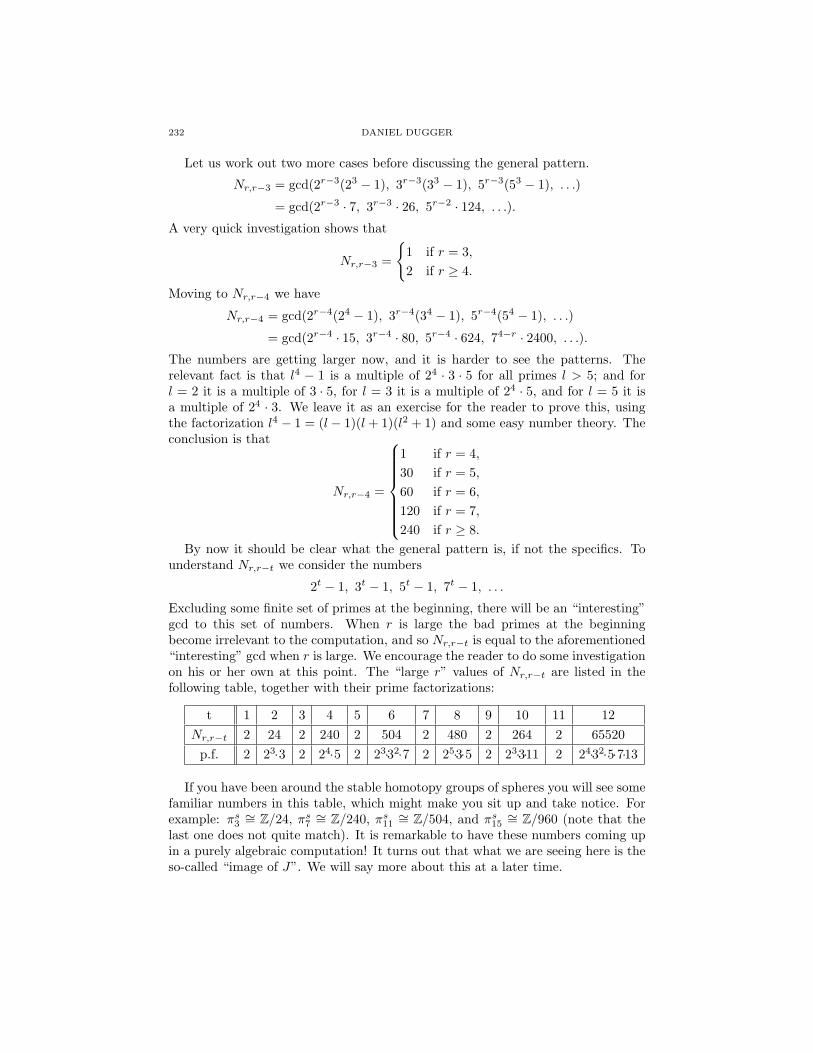
232 DANIEL DUGGER
Let us work out two more cases before discussing the general pattern.
Nr,r−3 = gcd(2r−3(23 − 1), 3r−3(33 − 1), 5r−3(53 − 1), . . .)
= gcd(2r−3 · 7, 3r−3 · 26, 5r−2 · 124, . . .).
A very quick investigation shows that
Nr,r−3 =
1 if r = 3,2 if r ≥ 4.
Moving to Nr,r−4 we have
Nr,r−4 = gcd(2r−4(24 − 1), 3r−4(34 − 1), 5r−4(54 − 1), . . .)
= gcd(2r−4 · 15, 3r−4 · 80, 5r−4 · 624, 74−r · 2400, . . .).
The numbers are getting larger now, and it is harder to see the patterns. Therelevant fact is that l4 − 1 is a multiple of 24 · 3 · 5 for all primes l > 5; and forl = 2 it is a multiple of 3 · 5, for l = 3 it is a multiple of 24 · 5, and for l = 5 it isa multiple of 24 · 3. We leave it as an exercise for the reader to prove this, usingthe factorization l4 − 1 = (l − 1)(l + 1)(l2 + 1) and some easy number theory. Theconclusion is that
Nr,r−4 =
1 if r = 4,30 if r = 5,60 if r = 6,120 if r = 7,240 if r ≥ 8.
By now it should be clear what the general pattern is, if not the specifics. Tounderstand Nr,r−t we consider the numbers
2t − 1, 3t − 1, 5t − 1, 7t − 1, . . .
Excluding some finite set of primes at the beginning, there will be an “interesting”gcd to this set of numbers. When r is large the bad primes at the beginningbecome irrelevant to the computation, and so Nr,r−t is equal to the aforementioned“interesting” gcd when r is large. We encourage the reader to do some investigationon his or her own at this point. The “large r” values of Nr,r−t are listed in thefollowing table, together with their prime factorizations:
t 1 2 3 4 5 6 7 8 9 10 11 12Nr,r−t 2 24 2 240 2 504 2 480 2 264 2 65520
p.f. 2 23·3 2 24·5 2 23·32·7 2 25·3·5 2 23·3·11 2 24·32·5·7·13
If you have been around the stable homotopy groups of spheres you will see somefamiliar numbers in this table, which might make you sit up and take notice. Forexample: πs3 ∼= Z/24, πs7 ∼= Z/240, πs11 ∼= Z/504, and πs15
∼= Z/960 (note that thelast one does not quite match). It is remarkable to have these numbers coming upin a purely algebraic computation! It turns out that what we are seeing here is theso-called “image of J”. We will say more about this at a later time.
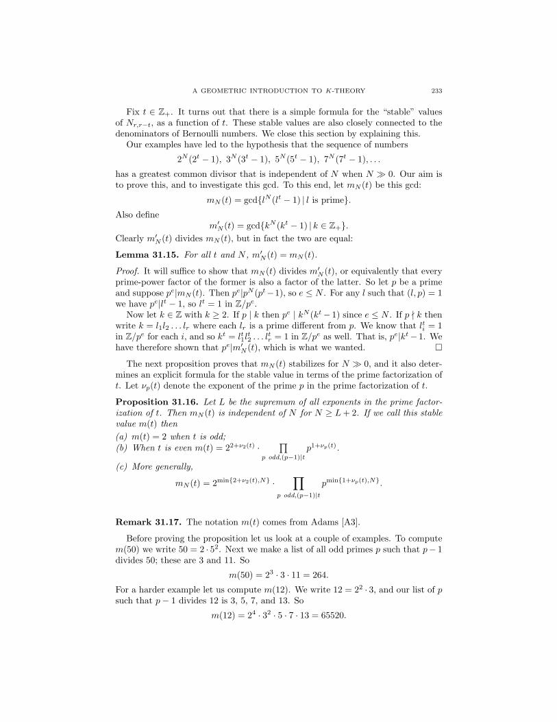
A GEOMETRIC INTRODUCTION TO K-THEORY 233
Fix t ∈ Z+. It turns out that there is a simple formula for the “stable” valuesof Nr,r−t, as a function of t. These stable values are also closely connected to thedenominators of Bernoulli numbers. We close this section by explaining this.
Our examples have led to the hypothesis that the sequence of numbers
2N (2t − 1), 3N (3t − 1), 5N (5t − 1), 7N (7t − 1), . . .
has a greatest common divisor that is independent of N when N 0. Our aim isto prove this, and to investigate this gcd. To this end, let mN (t) be this gcd:
mN (t) = gcdlN (lt − 1) | l is prime.Also define
m′N (t) = gcdkN (kt − 1) | k ∈ Z+.
Clearly m′N (t) divides mN (t), but in fact the two are equal:
Lemma 31.15. For all t and N , m′N (t) = mN (t).
Proof. It will suffice to show that mN (t) divides m′N (t), or equivalently that every
prime-power factor of the former is also a factor of the latter. So let p be a primeand suppose pe|mN (t). Then pe|pN (pt−1), so e ≤ N . For any l such that (l, p) = 1we have pe|lt − 1, so lt = 1 in Z/pe.
Now let k ∈ Z with k ≥ 2. If p | k then pe | kN (kt− 1) since e ≤ N . If p - k thenwrite k = l1l2 . . . lr where each lr is a prime different from p. We know that lti = 1in Z/pe for each i, and so kt = lt1l
t2 . . . l
tr = 1 in Z/pe as well. That is, pe|kt−1. We
have therefore shown that pe|m′N (t), which is what we wanted.
The next proposition proves that mN (t) stabilizes for N 0, and it also deter-mines an explicit formula for the stable value in terms of the prime factorization oft. Let νp(t) denote the exponent of the prime p in the prime factorization of t.
Proposition 31.16. Let L be the supremum of all exponents in the prime factor-ization of t. Then mN (t) is independent of N for N ≥ L+ 2. If we call this stablevalue m(t) then(a) m(t) = 2 when t is odd;(b) When t is even m(t) = 22+ν2(t) ·
∏p odd,(p−1)|t
p1+νp(t).
(c) More generally,
mN (t) = 2min2+ν2(t),N ·∏
p odd,(p−1)|t
pmin1+νp(t),N.
Remark 31.17. The notation m(t) comes from Adams [A3].
Before proving the proposition let us look at a couple of examples. To computem(50) we write 50 = 2 · 52. Next we make a list of all odd primes p such that p− 1divides 50; these are 3 and 11. So
m(50) = 23 · 3 · 11 = 264.
For a harder example let us compute m(12). We write 12 = 22 · 3, and our list of psuch that p− 1 divides 12 is 3, 5, 7, and 13. So
m(12) = 24 · 32 · 5 · 7 · 13 = 65520.
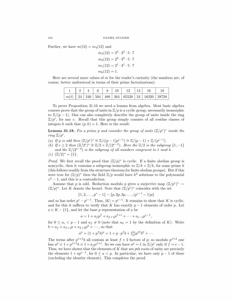
234 DANIEL DUGGER
Further, we have m(12) = m4(12) and
m3(12) = 23 · 32 · 5 · 7m2(12) = 22 · 32 · 5 · 7m1(12) = 21 · 31 · 5 · 7m0(12) = 1.
Here are several more values of m for the reader’s curiosity (the numbers are, ofcourse, better understood in terms of their prime factorizations):
t 2 4 6 8 10 12 14 16 18
m(t) 24 240 504 480 264 65520 24 16320 28728
To prove Proposition 31.16 we need a lemma from algebra. Most basic algebracourses prove that the group of units in Z/p is a cyclic group, necessarily isomorphicto Z/(p − 1). One can also completely describe the group of units inside the ringZ/pe, for any e. Recall that this group simply consists of all residue classes ofintegers k such that (p, k) = 1. Here is the result:
Lemma 31.18. Fix a prime p and consider the group of units (Z/pe)∗ inside thering Z/pe.(a) If p is odd then (Z/pe)∗ ∼= Z/((p− 1)pe−1) ∼= Z/(p− 1)× Z/(pe−1).(b) If e ≥ 2 then (Z/2e)∗ ∼= Z/2× Z/(2e−2). Here the Z/2 is the subgroup 1,−1
and the Z/(2e−2) is the subgroup of all numbers congruent to 1 mod 4.(c) (Z/2)∗ = 1.
Proof. We first recall the proof that (Z/p)∗ is cyclic. If a finite abelian group isnoncyclic, then it contains a subgroup isomorphic to Z/k × Z/k, for some prime k(this follows readily from the structure theorem for finite abelian groups). But if thiswere true for (Z/p)∗ then the field Z/p would have k2 solutions to the polynomialxk − 1, and this is a contradiction.
Assume that p is odd. Reduction modulo p gives a surjective map (Z/pe)∗ →(Z/p)∗. Let K denote the kernel. Note that (Z/pe)∗ coincides with the set
1, 2, . . . , pe − 1 − p, 2p, 3p, . . . , (pe−1 − 1)pand so has order pe− pe−1. Thus, |K| = pe−1. It remains to show that K is cyclic,and for this it suffices to verify that K has exactly p − 1 elements of order p. Leta ∈ K − 1, and let the base p representation of a be
a = 1 + afpf + af+1p
f+1 + · · ·+ ae−1pe−1,
for 0 ≤ ai < p − 1 and af 6= 0 (note that a0 = 1 by the definition of K). Writeb = af + af+1p+ af+2p
2 + · · · , so that
ap = (1 + pfb)p = 1 + p · pfb+(p2
)p2fb2 + · · ·
The terms after p1+fb all contain at least f + 2 factors of p; so modulo pf+2 onehas ap ≡ 1 + pf+1b ≡ 1 + afp
f+1. So we can have ap = 1 in Z/pe only if f = e− 1.Thus, we have shown that the elements of K that are pth roots of unity are preciselythe elements 1 + ape−1, for 0 ≤ a < p. In particular, we have only p − 1 of these(excluding the identity element). This completes the proof.
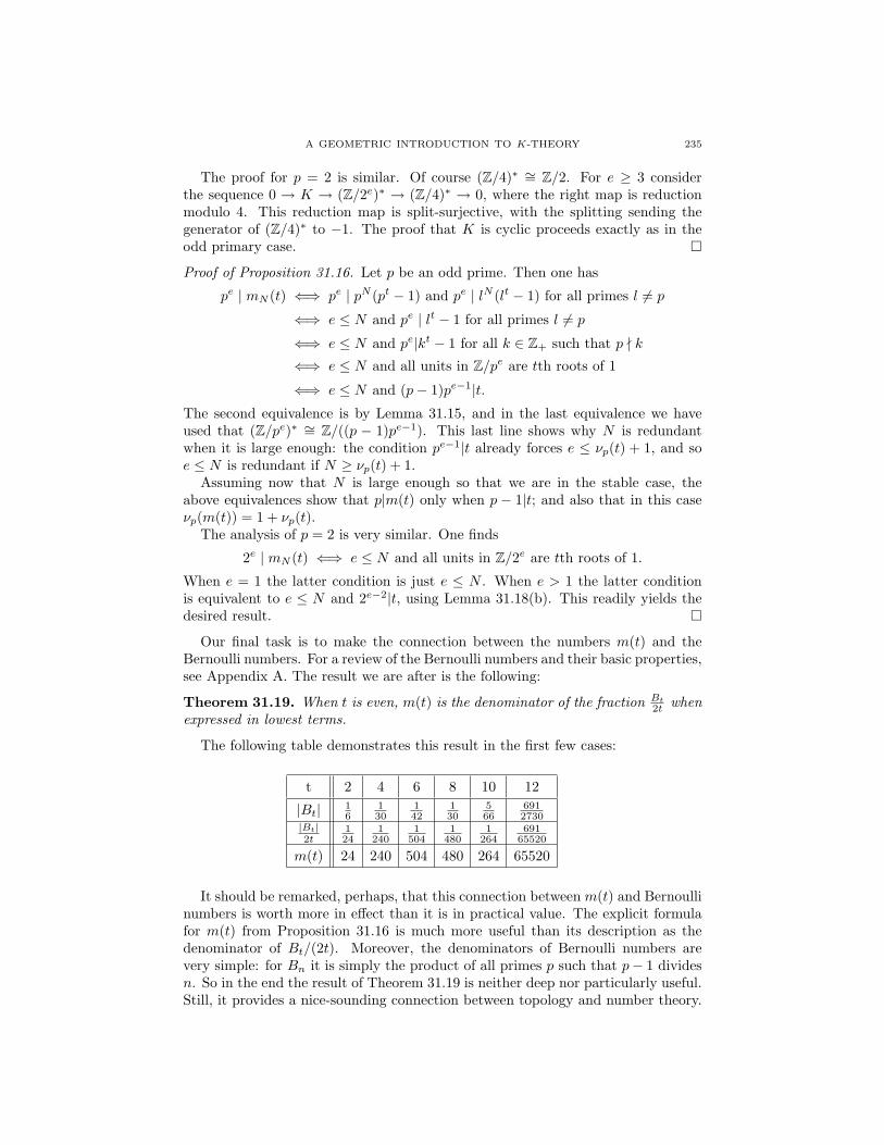
A GEOMETRIC INTRODUCTION TO K-THEORY 235
The proof for p = 2 is similar. Of course (Z/4)∗ ∼= Z/2. For e ≥ 3 considerthe sequence 0 → K → (Z/2e)∗ → (Z/4)∗ → 0, where the right map is reductionmodulo 4. This reduction map is split-surjective, with the splitting sending thegenerator of (Z/4)∗ to −1. The proof that K is cyclic proceeds exactly as in theodd primary case.
Proof of Proposition 31.16. Let p be an odd prime. Then one has
pe | mN (t) ⇐⇒ pe | pN (pt − 1) and pe | lN (lt − 1) for all primes l 6= p
⇐⇒ e ≤ N and pe | lt − 1 for all primes l 6= p
⇐⇒ e ≤ N and pe|kt − 1 for all k ∈ Z+ such that p - k⇐⇒ e ≤ N and all units in Z/pe are tth roots of 1
⇐⇒ e ≤ N and (p− 1)pe−1|t.The second equivalence is by Lemma 31.15, and in the last equivalence we haveused that (Z/pe)∗ ∼= Z/((p − 1)pe−1). This last line shows why N is redundantwhen it is large enough: the condition pe−1|t already forces e ≤ νp(t) + 1, and soe ≤ N is redundant if N ≥ νp(t) + 1.
Assuming now that N is large enough so that we are in the stable case, theabove equivalences show that p|m(t) only when p − 1|t; and also that in this caseνp(m(t)) = 1 + νp(t).
The analysis of p = 2 is very similar. One finds
2e | mN (t) ⇐⇒ e ≤ N and all units in Z/2e are tth roots of 1.
When e = 1 the latter condition is just e ≤ N . When e > 1 the latter conditionis equivalent to e ≤ N and 2e−2|t, using Lemma 31.18(b). This readily yields thedesired result.
Our final task is to make the connection between the numbers m(t) and theBernoulli numbers. For a review of the Bernoulli numbers and their basic properties,see Appendix A. The result we are after is the following:
Theorem 31.19. When t is even, m(t) is the denominator of the fraction Bt
2t whenexpressed in lowest terms.
The following table demonstrates this result in the first few cases:
t 2 4 6 8 10 12
|Bt| 16
130
142
130
566
6912730
|Bt|2t
124
1240
1504
1480
1264
69165520
m(t) 24 240 504 480 264 65520
It should be remarked, perhaps, that this connection between m(t) and Bernoullinumbers is worth more in effect than it is in practical value. The explicit formulafor m(t) from Proposition 31.16 is much more useful than its description as thedenominator of Bt/(2t). Moreover, the denominators of Bernoulli numbers arevery simple: for Bn it is simply the product of all primes p such that p− 1 dividesn. So in the end the result of Theorem 31.19 is neither deep nor particularly useful.Still, it provides a nice-sounding connection between topology and number theory.
236 DANIEL DUGGER
Proof of Proposition 31.19. By the theorem of von Staudt and Claussen (Theo-rem A.5) we know that the denominator of Bt (in lowest terms) is the product ofall primes p such that p − 1 divides t. Note that one such prime is p = 2, so thedenominator is even (in fact, congruent to 2 modulo 4) and the numerator is odd.Note also that these are the same primes appearing in the factorization of m(t), byProposition 31.16(b).
Consider now α = Bt/(2t). Since the numerator of Bt is odd, the number oftwos in the denominator of α is 1 + 1 + ν2(t). This is the same as the number oftwos in the prime factorization of m(t).
For every prime p such that p−1|t we have one p appearing in the denominator ofBt and νp(t) of them appearing in t, so the total number of p’s in the denominatorof α is 1 + νp(t). At this point we have thereby shown that m(t)|den(α).
It remains to check that if pe | t and p − 1 - t then pe divides the numerator ofBt and therefore disappears from the denominator of α. This is the nontrivial partof the proof.
Let p be an odd prime in the denominator of α, appearing with multiplicity e.Then pe is also in the denominator of Bt/t. By Proposition A.6 we know that
kt(kt−1)Bt
t ∈ Zfor all k ∈ Z. Consequently we have pe|kt(kt − 1) for all k ∈ Z. But this exactlysays that pe divides the gcd m(t). This verifies that the ‘odd part’ of den(α) dividesm(t), and we have already checked the factors of 2 in a previous paragraph. Soden(α) | m(t), and therefore the two are equal.
32. Calculation of KO for stunted projective spaces
The goal in this section is to determine KO0(RPn) and KO0(RPn/RP a) forall values of n and a, together with the Adams operations on these groups. Thesecomputations are the key to solving the vector field problem, which we do in the nextsection. As intermediate steps we also compute K∗(RPn) and K∗(RPn/RP a). Theoriginal written source for this material is Adams [Ad2] (although he acknowledgesunpublished work of Atiyah-Todd and Bott-Shapiro for portions of the calculation).We follow Adams’s approach very closely.
Some words of warning about this material are in order. The complete calcu-lation of KO for stunted projective spaces is fairly involved. Several things endup going on at once, so that there is a bunch of stuff to keep track of. And cal-culations are just never very fun to read in the first place. We have attempted tostructure our presentation to try to help with this, but of course it only goes so far.After some preliminary material we give a section which has just the statementsof the results, with a minimal amount of discussion in between (and no proofs).The intent is to give the reader the general picture, and also a convenient referencesection. All of the proofs are then given in a subsequent section.
Some readers might want to skip the proofs the first time through, and this isnot a problem. Later applications in the text only need the results, not details fromthe proofs. However, I highly recommend that algebraic topologists go throughthe proofs carefully at an early stage in their career. I cannot stress this enough.Going through the proofs will teach you something important about this subjectthat I do not have words for, and it will open up doors for you down the road.Trust me that this is an important thing to do.

A GEOMETRIC INTRODUCTION TO K-THEORY 237
32.1. Initial material. The results in this section will make heavy use of theinterplay between RPn and CPn in the homotopy category of spaces. We begin byreviewing the basics of what we will need.
Let η be the tautological complex line bundle on CPn, and let L be the tauto-logical real line bundle on RPn. Let j : RPn → CPn be the inclusion.
Lemma 32.2. The complexification of L is the pullback of η: that is, cL ∼= j∗η.
Proof. Complex line bundles on a space X are classified by homotopy classes in[X,CP∞]. The real line bundle L is classified by the inclusion RPn → RP∞, sothe complexificaton of L is classified by the composition RPn → RP∞ → CP∞.The complex line bundle η is classified by CPn → CP∞, so j∗η is classified bythe composition RPn → CPn → CP∞. The result follows from the commutativediagram
RPn //
CPn
RP∞ // CP∞.
Note that CP∞ ' K(Z, 2), so complex line bundles on X are classified by[X,CP∞] = H2(X). If n > 1 then H2(RPn) = Z/2, so there are only twoisomorphism classes of complex line bundles: the trivial bundle and the non-trivial bundle. The bundle cL = j∗η is nontrivial, since its classification mapRPn → RP∞ → CP∞ represents the generator of H2(RPn).
Remark 32.3. The powers ηk are all distinct line bundles on CPn (e.g., the firstChern classes are c1(ηk) = kc1(η) = kx where x is the generator of H2(CPn)). Thesituation upon pulling back to RPn is very different, however. We have
[j∗(η)]2 = (cL)2 = c(L2) = c(1R) = 1C.
So the even powers of j∗(η) are all trivial, and the odd powers are just j∗(η). Wewill see that this accounts for the main difference between K0(CPn) and K0(RPn).
In addition to the inclusion j : RPn → CPn there is another interesting map fromreal to complex projective space. Every real line in Cn+1 determines a complex lineby taking the C-linear span, and therefore we get a map PR(Cn+1)→ PC(Cn+1) =CPn. It is easy to see that this is a fiber bundle with fiber S1 (the space of reallines in C). Identifying Cn+1 with R2n+2 shows that the domain is homeomorphicto RP 2n+1, giving us a fiber bundle
S1 −→ RP 2n+1 q−→ CPn.In terms of homogeneous coordinates, q sends the point [x0 : x1 : · · · : x2n : x2n+1]to [x0 + ix1 : x2 + ix3 : · · · : x2n + ix2n+1].
Lemma 32.4. The diagram
RPni //
j %%JJJJJJJJJ RP 2n+1
q
CPn
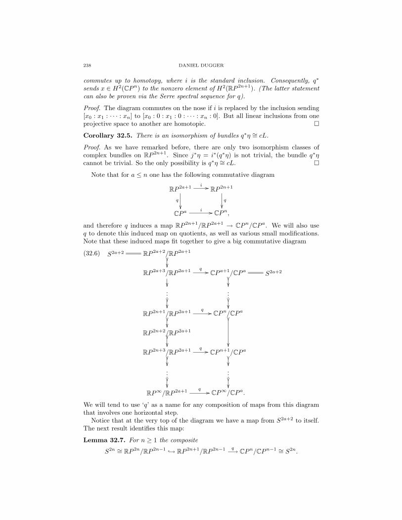
238 DANIEL DUGGER
commutes up to homotopy, where i is the standard inclusion. Consequently, q∗
sends x ∈ H2(CPn) to the nonzero element of H2(RP 2n+1). (The latter statementcan also be proven via the Serre spectral sequence for q).
Proof. The diagram commutes on the nose if i is replaced by the inclusion sending[x0 : x1 : · · · : xn] to [x0 : 0 : x1 : 0 : · · · : xn : 0]. But all linear inclusions from oneprojective space to another are homotopic.
Corollary 32.5. There is an isomorphism of bundles q∗η ∼= cL.
Proof. As we have remarked before, there are only two isomorphism classes ofcomplex bundles on RP 2n+1. Since j∗η = i∗(q∗η) is not trivial, the bundle q∗ηcannot be trivial. So the only possibility is q∗η ∼= cL.
Note that for a ≤ n one has the following commutative diagram
RP 2a+1 i //
q
RP 2n+1
q
CP a
i // CPn,
and therefore q induces a map RP 2n+1/RP 2a+1 → CPn/CP a. We will also useq to denote this induced map on quotients, as well as various small modifications.Note that these induced maps fit together to give a big commutative diagram
S2a+2 RP 2a+2/RP 2a+1
RP 2a+3/RP 2a+1 q //
CP a+1/CP a
S2a+2
...
...
RP 2n+1/RP 2a+1 q //
CPn/CP a
RP 2n+2/RP 2a+1
RP 2n+3/RP 2a+1 q //
CPn+1/CP a
...
...
RP∞/RP 2a+1 q // CP∞/CP a.
(32.6)
We will tend to use ‘q’ as a name for any composition of maps from this diagramthat involves one horizontal step.
Notice that at the very top of the diagram we have a map from S2a+2 to itself.The next result identifies this map:
Lemma 32.7. For n ≥ 1 the composite
S2n ∼= RP 2n/RP 2n−1 → RP 2n+1/RP 2n−1 q−→ CPn/CPn−1 ∼= S2n.

A GEOMETRIC INTRODUCTION TO K-THEORY 239
is a homeomorphism.
Proof. The space RP 2n/RP 2n−1 consists of the basepoint and the affine spaceR2n made up of points [x0 : x1 : · · · : x2n−2 : x2n−1 : 1]. Likewise, the spaceCPn/CPn−1 consists of the basepoint and the affine space Cn made up of thepoints [z0 : z1 : · · · : zn−1 : 1]. One readily uses the formula for q to see that it givesa bijective correspondence, and is therefore a homeomorphism.
32.8. The main results. Here we state the main theorems about the K-theoryof real and complex projective spaces. The proofs will be deferred until the nextsection.
Theorem 32.9 (Complex K-theory of complex projective spaces and stunted pro-jective spaces). Let η be the tautological line bundle on CPn, and write µ = [η]−1 ∈K0(CPn).(a) K0(CPn) = Z[µ]/(µn+1) and K1(CPn) = 0.(b) The Adams operations on K0(CPn) are given by
ψk(µs) =[(1 + µ)k − 1
]s = ksµs + s(k2
)µs+1 + (higher order terms).
(c) The sequence 0 → K0(CPn/CP a) → K0(CPn) → K0(CP a) → 0 is exact,and identifies K0(CPn/CP a) as the free abelian group Z〈µa+1, µa+2, . . . , µn〉 ⊆K0(CPn). The ring structure and action of the Adams operations are deter-mined by the corresponding structures on K0(CPn). Also, K1(CPn/CP a) = 0.
Remark 32.10. Following Adams [Ad2] we write µ(i) for the element ofK0(CPn/CP a) that maps to µi in K0(CPn). The extra parentheses in the ex-ponent remind us that this class is not a true ith power in the ring K0(CPn/CP a).
Theorem 32.11 (Complex K-theory of real projective spaces). Let ν be the ele-ment [j∗η]− 1 ∈ K0(RPn).(a) K0(RPn) ∼= Z/
(2b
n2 c)
with generator ν. The ring structure has ν2 = −2ν andνf+1 = 0, where f = bn2 c.
(b) K1(RPn) =
0 if n is evenZ if n is odd.
.
(c) The Adams operations on K0(RPn) are given by
ψk(νe) =
0 if k is evenνe if k is odd.
Recall that we have calculated K0(CPn/CP a−1) to be the free abelian groupZ〈µ(a), µ(a+1), . . . , µ(n)〉. For k ≤ 2n + 1 we may pull back these classes along themap q : RP k/RP 2a−1 → CPn/CP a−1 to get elements of K0(RP k/RP 2a−1). Weagain follow Adams [Ad2] and set
ν(t) = q∗(µ(t)) ∈ K0(RP k/RP 2a−1)
for a ≤ t ≤ n. Note that these elements correspond nicely as k and n vary, dueto the commutative diagram (32.6). We may as well take n 7→ ∞ so that we haveclasses ν(t) for all t ≥ a.
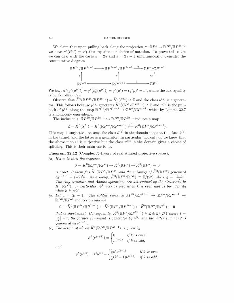
240 DANIEL DUGGER
We claim that upon pulling back along the projection π : RP k → RP k/RP 2a−1
we have π∗(ν(t)) = νt; this explains our choice of notation. To prove this claimwe can deal with the cases k = 2u and k = 2u + 1 simultaneously. Consider thecommutative diagram
RP 2u/RP 2a−1 // // RP 2u+1/RP 2a−1 q // CPu/CP a−1
RP 2u
π
OO
// // RP 2u+1q //
π
OO
CPu.
πC
OO
We have π∗(q∗(µ(t))) = q∗(π∗C(µ(t))) = q∗(µt) = (q∗µ)t = νt, where the last equalityis by Corollary 32.5.
Observe that K0(RP 2a/RP 2a−1) = K0(S2a) ∼= Z and the class ν(a) is a genera-tor. This follows because µ(a) generates K0(CP a/CP a−1) ∼= Z and ν(a) is the pull-back of µ(a) along the map RP 2a/RP 2a−1 → CP a/CP a−1, which by Lemma 32.7is a homotopy equivalence.
The inclusion i : RP 2a/RP 2a−1 → RPn/RP 2a−1 induces a map
Z = K0(S2a) = K0(RP 2a/RP 2a−1) i∗←− K0(RPn/RP 2a−1).
This map is surjective, because the class ν(a) in the domain maps to the class ν(a)
in the target, and the latter is a generator. In particular, not only do we know thatthe above map i∗ is surjective but the class ν(a) in the domain gives a choice ofsplitting. This is their main use to us.
Theorem 32.12 (Complex K-theory of real stunted projective spaces).(a) If a = 2t then the sequence
0→ K0(RPn/RP a)→ K0(RPn)→ K0(RP a)→ 0
is exact. It identifies K0(RPn/RP a) with the subgroup of K0(RPn) generatedby νt+1 = (−2)tν. As a group, K0(RPn/RP a) ∼= Z/(2g) where g = bn−a2 c.The ring structure and Adams operations are determined by the structures inK0(RPn). In particular, ψk acts as zero when k is even and as the identitywhen k is odd.
(b) Let a = 2t − 1. The cofiber sequence RP 2t/RP 2t−1 → RPn/RP 2t−1 →RPn/RP 2t induces a sequence
0← K0(RP 2t/RP 2t−1)← K0(RPn/RP 2t−1)← K0(RPn/RP 2t)← 0
that is short exact. Consequently, K0(RPn/RP 2t−1) ∼= Z⊕ Z/(2f ) where f =bn2 c − t; the former summand is generated by ν(t) and the latter summand isgenerated by ν(t+1).
(c) The action of ψk on K0(RPn/RP 2t−1) is given by
ψk(ν(t+1)) =
0 if k is evenν(t+1) if k is odd,
and
ψk(ν(t)) = ktν(t) +
12k
tν(t+1) if k is even12 (kt − 1)ν(t+1) if k is odd.
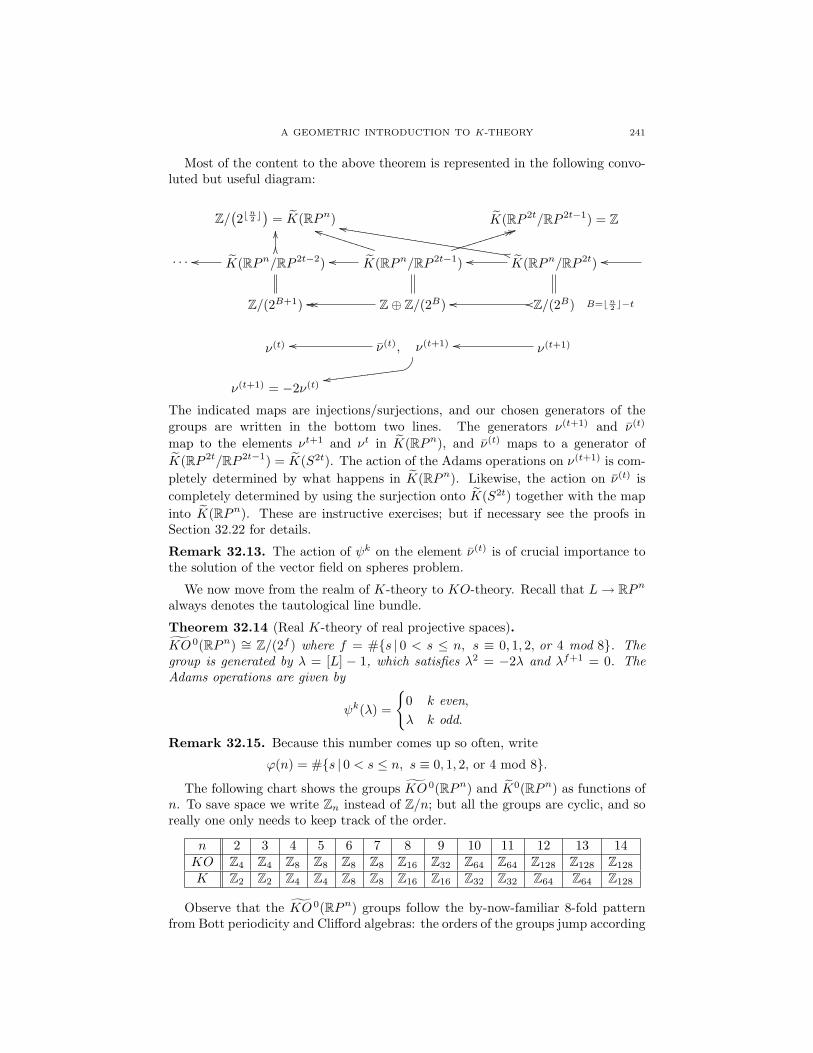
A GEOMETRIC INTRODUCTION TO K-THEORY 241
Most of the content to the above theorem is represented in the following convo-luted but useful diagram:
Z/(2b
n2 c)
= K(RPn) K(RP 2t/RP 2t−1) = Z
· · · K(RPn/RP 2t−2)
OOOO
oo K(RPn/RP 2t−1)oo
jjUUUUUUUUUU44 44iiiiiiiiiiiK(RPn/RP 2t)oo
ll
llZZZZZZZZZZZZZZZZZZZZZZZZZZoo
Z/(2B+1) Z⊕ Z/(2B)oooo Z/(2B)oooo B=bn2 c−t
ν(t) ν(t), ν(t+1)oo BCqqcccccccccccc
ν(t+1)oo
ν(t+1) = −2ν(t)
The indicated maps are injections/surjections, and our chosen generators of thegroups are written in the bottom two lines. The generators ν(t+1) and ν(t)
map to the elements νt+1 and νt in K(RPn), and ν(t) maps to a generator ofK(RP 2t/RP 2t−1) = K(S2t). The action of the Adams operations on ν(t+1) is com-pletely determined by what happens in K(RPn). Likewise, the action on ν(t) iscompletely determined by using the surjection onto K(S2t) together with the mapinto K(RPn). These are instructive exercises; but if necessary see the proofs inSection 32.22 for details.
Remark 32.13. The action of ψk on the element ν(t) is of crucial importance tothe solution of the vector field on spheres problem.
We now move from the realm of K-theory to KO-theory. Recall that L→ RPnalways denotes the tautological line bundle.
Theorem 32.14 (Real K-theory of real projective spaces).KO 0(RPn) ∼= Z/(2f ) where f = #s | 0 < s ≤ n, s ≡ 0, 1, 2, or 4 mod 8. Thegroup is generated by λ = [L] − 1, which satisfies λ2 = −2λ and λf+1 = 0. TheAdams operations are given by
ψk(λ) =
0 k even,λ k odd.
Remark 32.15. Because this number comes up so often, write
ϕ(n) = #s | 0 < s ≤ n, s ≡ 0, 1, 2, or 4 mod 8.
The following chart shows the groups KO 0(RPn) and K0(RPn) as functions ofn. To save space we write Zn instead of Z/n; but all the groups are cyclic, and soreally one only needs to keep track of the order.
n 2 3 4 5 6 7 8 9 10 11 12 13 14KO Z4 Z4 Z8 Z8 Z8 Z8 Z16 Z32 Z64 Z64 Z128 Z128 Z128
K Z2 Z2 Z4 Z4 Z8 Z8 Z16 Z16 Z32 Z32 Z64 Z64 Z128
Observe that the KO 0(RPn) groups follow the by-now-familiar 8-fold patternfrom Bott periodicity and Clifford algebras: the orders of the groups jump according
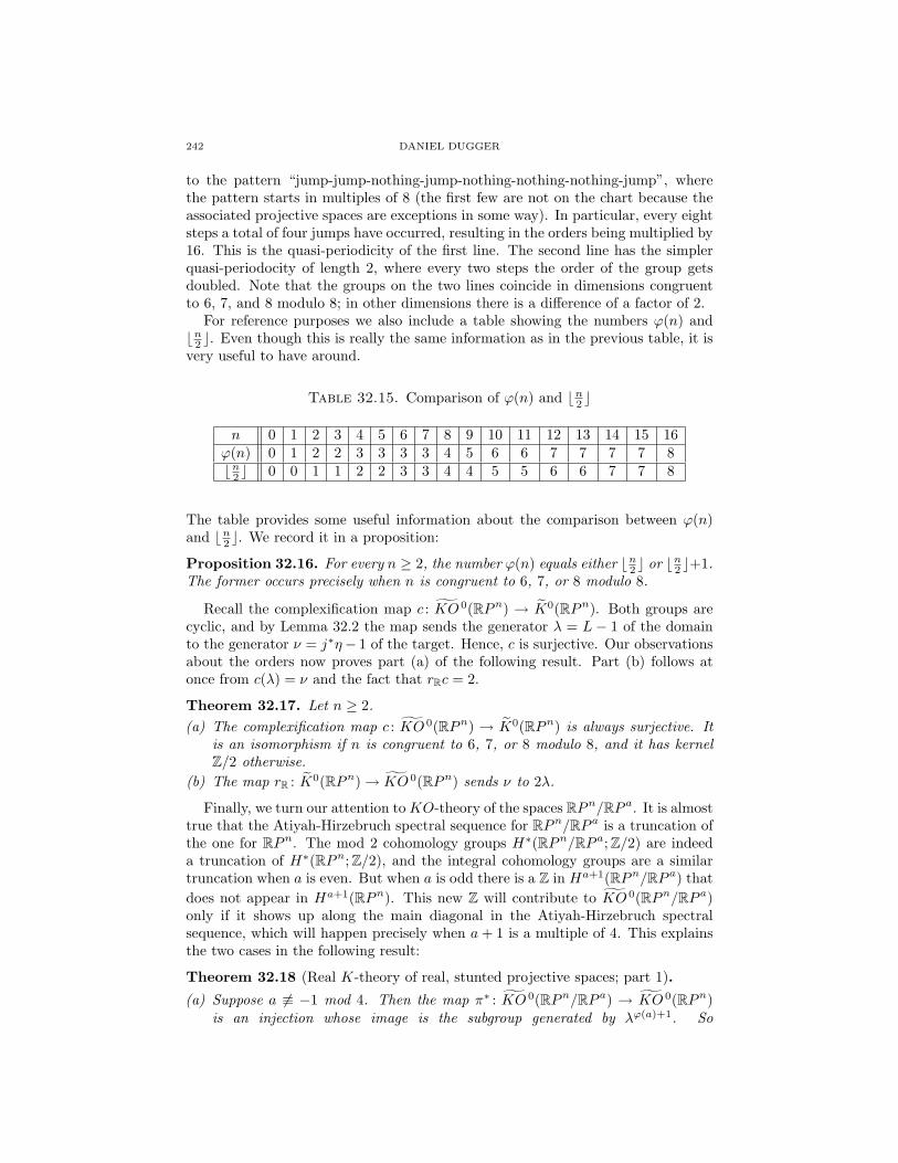
242 DANIEL DUGGER
to the pattern “jump-jump-nothing-jump-nothing-nothing-nothing-jump”, wherethe pattern starts in multiples of 8 (the first few are not on the chart because theassociated projective spaces are exceptions in some way). In particular, every eightsteps a total of four jumps have occurred, resulting in the orders being multiplied by16. This is the quasi-periodicity of the first line. The second line has the simplerquasi-periodocity of length 2, where every two steps the order of the group getsdoubled. Note that the groups on the two lines coincide in dimensions congruentto 6, 7, and 8 modulo 8; in other dimensions there is a difference of a factor of 2.
For reference purposes we also include a table showing the numbers ϕ(n) andbn2 c. Even though this is really the same information as in the previous table, it isvery useful to have around.
Table 32.15. Comparison of ϕ(n) and bn2 c
n 0 1 2 3 4 5 6 7 8 9 10 11 12 13 14 15 16ϕ(n) 0 1 2 2 3 3 3 3 4 5 6 6 7 7 7 7 8bn2 c 0 0 1 1 2 2 3 3 4 4 5 5 6 6 7 7 8
The table provides some useful information about the comparison between ϕ(n)and bn2 c. We record it in a proposition:
Proposition 32.16. For every n ≥ 2, the number ϕ(n) equals either bn2 c or bn2 c+1.The former occurs precisely when n is congruent to 6, 7, or 8 modulo 8.
Recall the complexification map c : KO 0(RPn) → K0(RPn). Both groups arecyclic, and by Lemma 32.2 the map sends the generator λ = L − 1 of the domainto the generator ν = j∗η− 1 of the target. Hence, c is surjective. Our observationsabout the orders now proves part (a) of the following result. Part (b) follows atonce from c(λ) = ν and the fact that rRc = 2.
Theorem 32.17. Let n ≥ 2.(a) The complexification map c : KO 0(RPn) → K0(RPn) is always surjective. It
is an isomorphism if n is congruent to 6, 7, or 8 modulo 8, and it has kernelZ/2 otherwise.
(b) The map rR : K0(RPn)→ KO 0(RPn) sends ν to 2λ.
Finally, we turn our attention toKO-theory of the spaces RPn/RP a. It is almosttrue that the Atiyah-Hirzebruch spectral sequence for RPn/RP a is a truncation ofthe one for RPn. The mod 2 cohomology groups H∗(RPn/RP a; Z/2) are indeeda truncation of H∗(RPn; Z/2), and the integral cohomology groups are a similartruncation when a is even. But when a is odd there is a Z in Ha+1(RPn/RP a) thatdoes not appear in Ha+1(RPn). This new Z will contribute to KO 0(RPn/RP a)only if it shows up along the main diagonal in the Atiyah-Hirzebruch spectralsequence, which will happen precisely when a+ 1 is a multiple of 4. This explainsthe two cases in the following result:
Theorem 32.18 (Real K-theory of real, stunted projective spaces; part 1).
(a) Suppose a 6≡ −1 mod 4. Then the map π∗ : KO 0(RPn/RP a) → KO 0(RPn)is an injection whose image is the subgroup generated by λϕ(a)+1. So
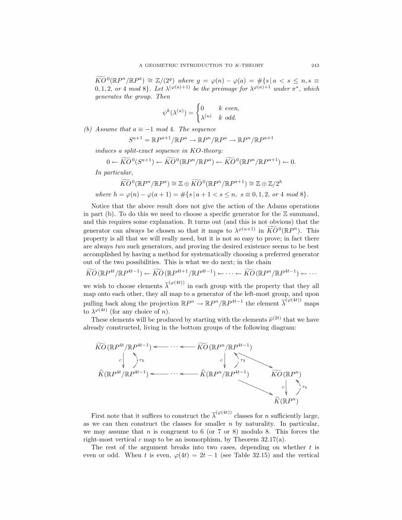
A GEOMETRIC INTRODUCTION TO K-THEORY 243
KO 0(RPn/RP a) ∼= Z/(2g) where g = ϕ(n) − ϕ(a) = #s | a < s ≤ n, s ≡0, 1, 2, or 4 mod 8. Let λ(ϕ(a)+1) be the preimage for λϕ(a)+1 under π∗, whichgenerates the group. Then
ψk(λ(u)) =
0 k even,λ(u) k odd.
(b) Assume that a ≡ −1 mod 4. The sequence
Sa+1 = RP a+1/RP a → RPn/RP a → RPn/RP a+1
induces a split-exact sequence in KO-theory:
0← KO 0(Sa+1)← KO 0(RPn/RP a)← KO 0(RPn/RP a+1)← 0.
In particular,
KO 0(RPn/RP a) ∼= Z⊕ KO 0(RPn/RP a+1) ∼= Z⊕ Z/2h
where h = ϕ(n)− ϕ(a+ 1) = #s | a+ 1 < s ≤ n, s ≡ 0, 1, 2, or 4 mod 8.
Notice that the above result does not give the action of the Adams operationsin part (b). To do this we need to choose a specific generator for the Z summand,and this requires some explanation. It turns out (and this is not obvious) that thegenerator can always be chosen so that it maps to λϕ(a+1) in KO 0(RPn). Thisproperty is all that we will really need, but it is not so easy to prove; in fact thereare always two such generators, and proving the desired existence seems to be bestaccomplished by having a method for systematically choosing a preferred generatorout of the two possibilities. This is what we do next; in the chain
KO (RP 4t/RP 4t−1)← KO (RP 4t+1/RP 4t−1)← · · · ← KO (RPn/RP 4t−1)← · · ·
we wish to choose elements λ(ϕ(4t))
in each group with the property that they allmap onto each other, they all map to a generator of the left-most group, and uponpulling back along the projection RPn → RPn/RP 4t−1 the element λ
(ϕ(4t))maps
to λϕ(4t) (for any choice of n).These elements will be produced by starting with the elements ν(2t) that we have
already constructed, living in the bottom groups of the following diagram:
KO (RP 4t/RP 4t−1)
c
· · ·oo KO (RPn/RP 4t−1)oo
c
((QQQQQQQQQQQQ
K(RP 4t/RP 4t−1)
rR
aa
· · ·oo K(RPn/RP 4t−1)oo
rR
aa
((QQQQQQQQQQQQKO (RPn)
c
K(RPn)
rR
aa
First note that it suffices to construct the λ(ϕ(4t))
classes for n sufficiently large,as we can then construct the classes for smaller n by naturality. In particular,we may assume that n is congruent to 6 (or 7 or 8) modulo 8. This forces theright-most vertical c map to be an isomorphism, by Theorem 32.17(a).
The rest of the argument breaks into two cases, depending on whether t iseven or odd. When t is even, ϕ(4t) = 2t − 1 (see Table 32.15) and the vertical
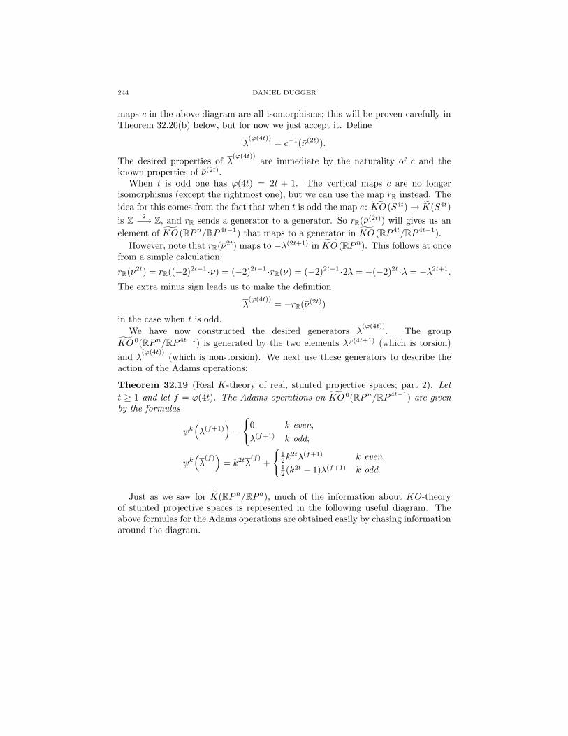
244 DANIEL DUGGER
maps c in the above diagram are all isomorphisms; this will be proven carefully inTheorem 32.20(b) below, but for now we just accept it. Define
λ(ϕ(4t))
= c−1(ν(2t)).
The desired properties of λ(ϕ(4t))
are immediate by the naturality of c and theknown properties of ν(2t).
When t is odd one has ϕ(4t) = 2t + 1. The vertical maps c are no longerisomorphisms (except the rightmost one), but we can use the map rR instead. Theidea for this comes from the fact that when t is odd the map c : KO (S4t)→ K(S4t)is Z 2−→ Z, and rR sends a generator to a generator. So rR(ν(2t)) will gives us anelement of KO (RPn/RP 4t−1) that maps to a generator in KO (RP 4t/RP 4t−1).
However, note that rR(ν2t) maps to −λ(2t+1) in KO (RPn). This follows at oncefrom a simple calculation:
rR(ν2t) = rR((−2)2t−1 ·ν) = (−2)2t−1 ·rR(ν) = (−2)2t−1 ·2λ = −(−2)2t ·λ = −λ2t+1.
The extra minus sign leads us to make the definition
λ(ϕ(4t))
= −rR(ν(2t))
in the case when t is odd.We have now constructed the desired generators λ
(ϕ(4t)). The group
KO 0(RPn/RP 4t−1) is generated by the two elements λϕ(4t+1) (which is torsion)and λ
(ϕ(4t))(which is non-torsion). We next use these generators to describe the
action of the Adams operations:
Theorem 32.19 (Real K-theory of real, stunted projective spaces; part 2). Lett ≥ 1 and let f = ϕ(4t). The Adams operations on KO 0(RPn/RP 4t−1) are givenby the formulas
ψk(λ(f+1)
)=
0 k even,λ(f+1) k odd;
ψk(λ
(f))
= k2tλ(f)
+
12k
2tλ(f+1) k even,12 (k2t − 1)λ(f+1) k odd.
Just as we saw for K(RPn/RP a), much of the information about KO-theoryof stunted projective spaces is represented in the following useful diagram. Theabove formulas for the Adams operations are obtained easily by chasing informationaround the diagram.
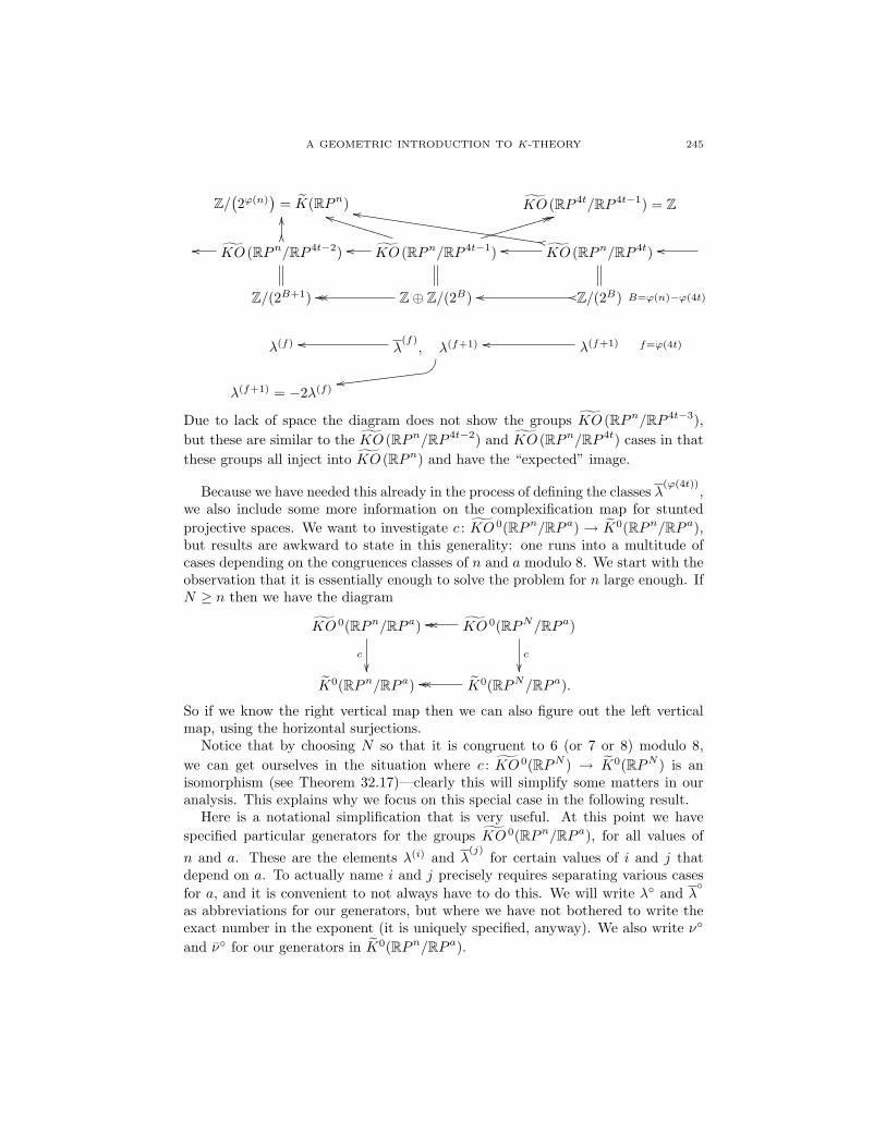
A GEOMETRIC INTRODUCTION TO K-THEORY 245
Z/(2ϕ(n)
)= K(RPn) KO (RP 4t/RP 4t−1) = Z
KO (RPn/RP 4t−2)
OOOO
oo KO (RPn/RP 4t−1)oo
jjUUUUUUUUUU44 44hhhhhhhhhhh
KO (RPn/RP 4t)oomm
mmZZZZZZZZZZZZZZZZZZZZZZZZZZoo
Z/(2B+1) Z⊕ Z/(2B)oooo Z/(2B)oooo B=ϕ(n)−ϕ(4t)
λ(f) λ(f), λ(f+1)oo BC
qqcccccccccccc
λ(f+1)oo f=ϕ(4t)
λ(f+1) = −2λ(f)
Due to lack of space the diagram does not show the groups KO (RPn/RP 4t−3),but these are similar to the KO (RPn/RP 4t−2) and KO (RPn/RP 4t) cases in thatthese groups all inject into KO (RPn) and have the “expected” image.
Because we have needed this already in the process of defining the classes λ(ϕ(4t))
,we also include some more information on the complexification map for stuntedprojective spaces. We want to investigate c : KO 0(RPn/RP a) → K0(RPn/RP a),but results are awkward to state in this generality: one runs into a multitude ofcases depending on the congruences classes of n and a modulo 8. We start with theobservation that it is essentially enough to solve the problem for n large enough. IfN ≥ n then we have the diagram
KO 0(RPn/RP a)
c
KO 0(RPN/RP a)
c
oooo
K0(RPn/RP a) K0(RPN/RP a).oooo
So if we know the right vertical map then we can also figure out the left verticalmap, using the horizontal surjections.
Notice that by choosing N so that it is congruent to 6 (or 7 or 8) modulo 8,we can get ourselves in the situation where c : KO 0(RPN ) → K0(RPN ) is anisomorphism (see Theorem 32.17)—clearly this will simplify some matters in ouranalysis. This explains why we focus on this special case in the following result.
Here is a notational simplification that is very useful. At this point we havespecified particular generators for the groups KO 0(RPn/RP a), for all values ofn and a. These are the elements λ(i) and λ
(j)for certain values of i and j that
depend on a. To actually name i and j precisely requires separating various casesfor a, and it is convenient to not always have to do this. We will write λ and λ
as abbreviations for our generators, but where we have not bothered to write theexact number in the exponent (it is uniquely specified, anyway). We also write ν
and ν for our generators in K0(RPn/RP a).

246 DANIEL DUGGER
Theorem 32.20. Consider the map c : KO 0(RPn/RP a) → K0(RPn/RP a) andthe map rR going in the opposite direction. Assume that n is congruent to 6, 7, or8 modulo 8.(a) Suppose a is even, so that both the groups are torsion.
(i) If a ≡ 6, 8 mod 8 then c is an isomorphism, c(λ) = ν, and rR(ν) = 2λ.(ii) If a ≡ 2, 4 mod 8 then c is an injection with cokernel Z/2. One has
c(λ) = −2ν and rR(ν) = −λ.(b) Suppose that a = 4t− 1. Here both the domain and target of c have copies of Z
inside them.(i) If a ≡ 7 mod 8 (i.e., t is even) then c is an isomorphism.(ii) If a ≡ 3 mod 8 (i.e., t is odd) then c is a monomorphism, and the cokernel
is Z/2⊕ Z/2.(c) Suppose that a = 4t + 1. In this case c maps its domain isomorphically onto
the torsion subgroup of the target of c. One has c(λ) = ν and rR(ν) = 2λ.
32.21. An extended example. Let us demonstrate much of what we have learnedby looking at a specific example. The Atiyah-Hirzebruch spectral sequence forcomputing KO (RP 10) gives one Z/2 for every dimension from 1 through 10 thatis congruent to 0, 1, 2, or 4 modulo 8. These are the dimensions 1, 2, 4, 8, 9, and10—so we have six Z/2’s, and KO (RP 10) ∼= Z/(26). In comparison, K(RP 10) isjust Z/(25) (as 5 = 10
2 ).There is a visual way of representing this information that is useful, especially
when it comes to the stunted projective spaces. Draw a cell diagram for RP 10,leaving out the 0-cell. For KO (RP 10) discard all cells except the ones in dimensionscongruent to 0, 1, 2, or 4 modulo 8; then label the remaining cells with ascendingpowers of λ. For K(RP 10) discard all the odd-dimensional cells and label theremaining ones with ascending powers of ν. Always remembering that λ2 = −2λ(and ν2 = −2ν), the cells now represent the associated graded of KO (RP 10) (orK(RP 10)) with respect to the 2-adic filtration. The picture below also shows thecomplexification map c : KO (RP 10) → K(RP 10). Recall that this is a ring mapand sends λ to ν:
gKO (RP 10)c−→ eK(RP 10)
λ
λ2
λ3
λ4
λ5
λ6
ν
ν2
ν3
ν4
ν5
We see in this case that c : KO (RP 10)→ K(RP 10) is surjective with kernel Z/2(generated by λ6 = −32λ). One has rR(ν) = rR(c(λ)) = 2λ, and more generally
rR(νk) = rR((−2)k−1ν) = (−2)k−1rR(ν) = (−2)k−1 · 2λ = −(−2)kλ = −λk+1.

A GEOMETRIC INTRODUCTION TO K-THEORY 247
Next let us consider the K-groups of RP 10/RP 4, referring to the diagram
KO (RP 10/RP 4)
c
// // KO (RP 10)
c
K(RP 10/RP 4) // // K(RP 10).
In relation to our cell-diagrams, the K-groups of RP 10/RP 4 are obtained by throw-ing away the bottom four cells. We obtain the picture
gKO (RP 10/RP 4)c−→ eK(RP 10/RP 4)
λ(4)
λ(5)
λ(6)
ν(3)
ν(4)
ν(5)
This picture tells us that KO (RP 10/RP 4) ∼= Z/(23), generated by λ(4), and alsoK(RP 10/RP 4) ∼= Z/(23) with generator ν(3). These each embed into the respectiveK-group of RP 10. The complexification map therefore sends λ(4) to ν(4), and wefind that this map has both kernel and cokernel isomorphic to Z/2.
The situation is a little different if we consider the K-groups of RP 10/RP 3.Here the bottom cell of RP 10/RP 3 gives rise to a Z in singular cohomology, and acorresponding Z in the K-groups. The picture becomes as follows:
gKO (RP 10/RP 3)c−→ eK(RP 10/RP 3)
λ(3)
λ(4)
λ(5)λ(6)
−2ν(2)
ν(3)
ν(4)
ν(5)
Here the black dots represent copies of Z, so that KO (RP 10/RP 3) ∼= Z ⊕ Z/8with the two summands generated by λ
(3)and λ(4), respectively. Likewise,
K(RP 10/RP 3) ∼= Z ⊕ Z/8 with the two summands generated by ν(2) and ν(3).The various maps
KO (RP 10/RP 4) −→ KO (RP 10/RP 3) −→ KO (RP 10), and
K(RP 10/RP 4) −→ K(RP 10/RP 3) −→ K(RP 10)
are the evident ones suggested by the diagrams. The only subtlety lies in deter-mining the complexification map c. Of course c(λ(i)) = ν(i) for i = 4, 5, as this isforced by that happens on the subgroup KO (RP 10/RP 4) ⊆ KO (RP 10/RP 3). Tocompute c(λ
(3)) we must remember that λ
(3)is defined by the equation
λ(3)
= −rR(ν(2))
248 DANIEL DUGGER
(note that 3 = 4t− 1 where t = 1, and so we are in the case where t is odd; in thecase where t is even the definition of the λ classes is different). So we obtain
c(λ
(3))= −c(rR(ν(2))) = −(1 + ψ−1)(ν(2)) = −[ν(2) + ν(2)] = −2ν(2).
Here we have used Theorem 32.12(c) for evaluating ψ−1(ν(2)). Note that the pull-back map induced by RP 10 → RP 10/RP 3 sends λ
(3)to λ3 and sends −2ν(2) to
−2ν2 = ν3; hence the above formula is consistent with our previous computationof c : KO (RP 10)→ K(RP 10).
32.22. The proofs. We now give proofs for all of the results previously stated inthis section.
Proof of Theorem 32.9. This is straightforward, and left to the reader.
Proof of Theorem 32.11. There is no room for differentials in the Atiyah-Hirzebruch spectral sequence for K∗(RPn), so it collapses at E2. Part (b) followsimmediately. It is also a direct consequence that K0(RPn) is an abelian group oforder 2b
n2 c. It remains to solve the extension problems to determine precisely which
group it is.Observe that L2 = 1, hence (cL)2 = c(L2) = c(1) = 1. So
ν2 = (cL− 1)2 = (cL)2 − 2(cL) + 1 = 2(1− c(L)) = −2ν.
Note that an immediate consequence is νt = (−2)t−1ν.Let F i = ker
(K0(RPn)→ K0(RP i−1)
). So
K0(RPn) = F 0 ⊇ F 1 ⊇ F 2 ⊇ · · · ⊇ Fn+1 = 0.
The quotients F i/F i+1 are the groups in the E∞ term of the spectral sequence,and so are
F i/F i+1 =
Z/2 0 < i ≤ 2bn2 c and i even0 otherwise.
So F 0 = F 1 = F 2 and F 2/F 3 ∼= Z/2. The element ν generates F 2/F 3: weknow this by naturality of the spectral sequence, applied to the map j : RPn →CPn. The element µ generates F 2/F 3 for K0(CPn), and H2(CPn) → H2(RPn)is the projection Z → Z/2: the image of a generator is another generator. So j∗µgenerates F 2/F 3 for K0(RPn), and of course ν = j∗µ.
The multiplicativity of the spectral sequence then gives us that ν2 generatesF 4/F 5, and in general νj generates F 2j/F 2j+1 for j = 1, 2, . . . , bn2 c. In particular,νj is not equal to zero for j in this range. But νj = (−2)j−1ν, so 2b
n2 c−1ν 6= 0. This
proves that the only possibility for K0(RPn) is Z/2bn2 c, and that ν is a generator.
Note that we than have 0 = (−2)bn2 cν = νb
n2 c+1.
For part (c) we just observe that ψk(cL) = (cL)k = c(Lk) and this equals 1 if kis even, and cL if k is odd.
Proof of Theorem 32.12. Parts (a) and (b) are trivial. In each case one writesdown the evident long exact sequence and quickly sees that the given sequenceis short exact. The only slight subtlety is seeing in the case a = 2t − 1 thatK0(RPn/RP 2t−1)→ K0(RP 2t/RP 2t−1) is surjective, but this was explained whenwe constructed the element ν(t) (which maps to a generator in the target group).
A GEOMETRIC INTRODUCTION TO K-THEORY 249
For part (c), the action of ψk on ν(t+1) is determined by the corresponding actionin K0(RPn/RP 2t); so there is nothing to prove here. The action on ν(t) is moreinteresting. We can, of course, write
ψk(ν(t)) = Aν(t) +Bν(t+1)(32.23)
where A is a unique integer and B is unique modulo 2f . Applying the mapi∗ : K0(RPn/RP 2t−1) → K0(RP 2t/RP 2t−1) kills ν(t+1) and sends ν(t) to a gen-erator g, so this equation becomes ψk(g) = Ag. But we already know that ψk actson such a generator by kt, so A = kt.
Next we apply the map π∗ : K0(RPn/RP 2t) → K0(RPn) to equation (32.23).The map π∗ sends ν(t) to νt and ν(t+1) to νt+1, so using A = kt we obtain
ψk(νt) = ktνt +Bνt+1
in K0(RPn). Now use that ψk is a ring homomorphism, together with νt+1 = −2νt.We get
(kt − 2B)νt =[ψk(ν)
]t =
0 if k is evenνt if k is odd.
The group K0(RPn) is Z/(2g) with generator ν, and νt = (−2)t−1ν. So theadditive order of νt is 2g−t+1, or equivalently 2f+1. In the case that k is even itfollows that kt − 2B is a multiple of 2f+1, so that kt
2 ≡ B mod 2f (recall that B isonly well-defined modulo 2f in the first place).
In the remaining case where k is odd we get kt − 2B ≡ 1 modulo 2f+1. Sokt−1
2 ≡ B modulo 2f , which is what we wanted.
Proof of Theorem 32.14. In the Atiyah-Hirzebruch spectral sequence forKO (RPn), the diagonal of the E2-term that is relevant to KO 0(RPn) consistsof ϕ(n) copies of Z/2. The first concern is to determine if there are any differentialscausing some of these copies to disappear by E∞, and the second concern is theproblem of extensions.
Observe that the complexification map c : KO 0(RPn)→ K0(RPn) is surjective,because ν generates the target and ν = c(L− 1). So it follows from Theorem 32.11that at least bn2 c among our ϕ(n) copies of Z/2 must survive the spectral sequence.
The trick now is to not consider one n at a time, but rather to consider themall at once. When n is congruent to 6, 7, or 8 modulo 8 then we know ϕ(n) = bn2 c,and so here it must be that all the Z/2’s along the main diagonal survive. Thatis, all differentials entering or exiting the main diagonal are zero. But then bynaturality of the spectral sequence this is true for all n. We conclude that the orderof KO 0(RPn) is 2ϕ(n), no matter what n is.
When n is congruent to 6, 7, or 8 modulo 8 we now know that the ordersof KO 0(RPn) and K0(RPn) are the same. Since the complexification map issurjective, it is therefore an isomorphism. So KO 0(RPn) is cyclic. Since c(λ) = νit follows that λ is a generator. In particular, λ is a generator for the quotientF 1/F 2.
But then by naturality of the spectral sequence (and with it, naturality of thefiltration F i) it follows that λ generates F 1/F 2 for every value of n. Since L2 = 1we of course have λ2 = −2λ. At this point the argument follows the one in theproof of Theorem 32.11 to show that KO 0(RPn) is cyclic, for all values of n.
250 DANIEL DUGGER
The computation of the Adams operations again follows from ψk(L) = Lk, whichequals 1 if k is even and L if k is odd.
Proof of Theorem 32.17. This was given just prior to the statement of the theorem.
Proof of Theorem 32.18. For part (a) one examines the Atiyah-Hirzebruch spectralsequence for KO ∗(RPn/RP a). Note that the quotient RPn → RPn/RP a inducesa map of spectral sequences in the other direction. The diagonal groups in the E2-term for KO ∗(RPn/RP a) are a truncation of the diagonal groups appearing in theE2-term for KO ∗(RPn). Since there are no entering or exiting differentials (alongthe diagonal) in the latter case, naturality of the spectral sequence guarantees thereare no entering or exiting differentials for RPn/RP a. Passing to E∞-terms now,we see that the associated graded groups for KO (RPn/RP a) are a truncation ofthe associated graded groups for KO (RPn). Examining the map of filtered groups
KO (RPn/RP a)
π∗
F1
oooo F2oooo
· · ·oooo
KO (RPn) F ′1oooo F ′2oooo · · ·oooo
we now find that Fk → F ′k is an isomorphism for k ≥ a + 1 and Fk/Fk+1 = 0for k ≤ a. It follows that KO (RPn/RP a) → KO (RPn) is an injection, withimage equal to F ′a+1. In our analysis of KO(RPn) we have already seen thatF ′a+1 ⊆ KO (RPn) is the subgroup generated by λa+1. Everything else in part (a)is then immediate.
For (b) we only need to prove that KO 0(RPn/RP 4t−1)→ KO 0(RP 4t/RP 4t−1)is surjective, since the latter group is isomorphic to KO 0(S4t) ∼= Z. Everythingelse in part (b) is routine. To do this, consider the following diagram:
Z/2
· · · KO 1(RPn/RP 4t)oo KO 0(RP 4t/RP 4t−2)oo KO 0(RPn/RP 4t−2)j∗1oooo · · ·oo
· · · KO 1(RPn/RP 4t)oo
OO
KO 0(RP 4t/RP 4t−1)oo
i∗OOOO
KO 0(RPn/RP 4t−1)j∗2oo
OOOO
· · ·oo
ZThe two indicated vertical maps are surjections because they sit inside long exactsequences where the third term is KO 0(RP 4t−1/RP 4t−2) = KO 0(S4t−1) = 0. Theindicated group is Z/2 by part (a) of the theorem, which also yields the diagram
KO 0(RP 4t) KO 0(RPn)oooo
KO 0(RP 4t/RP 4t−2)
OO
OO
KO 0(RPn/RP 4t−2).
OO
OO
j∗1oo
A GEOMETRIC INTRODUCTION TO K-THEORY 251
The group KO 0(RP 4t/RP 4t−2) is the subgroup of KO 0(RP 4t) generatedby ν1+ϕ(4t−2), and KO 0(RPn/RP 4t−2) is the similarly-described subgroup ofKO 0(RPn). It follows at once that j∗1 is surjective.
Returning to the earlier diagram, the image of j∗2 is an ideal (r) inside of Z. Thefact that i∗j∗2 is surjective (readily observed from the diagram) proves that r mustbe odd. But the quotient Z/r will inject into KO 1(RPn/RP 4t), by the long exactsequence. The Atiyah-Hirzebruch spectral sequence shows that this latter grouphas no odd torsion, because it has a filtration where the quotients are only Z’s andZ/2’s. So the conclusion is that r = 1, hence j∗2 is surjective.
Proof of Theorem 32.19. The evaluation of ψk(λ(f+1)
)is immediate using natural-
ity and Theorem 32.14. For the evaluation of ψk(λ
(f))
one can repeat the proofof Theorem 32.12(c) almost verbatim. Alternatively, one can use the result of The-orem 32.12(c) together with the complexification map c : KO 0(RPn/RP 4t−1) →K0(RPn/RP 4t−1), which is a monomorphism for n congruent to 6, 7, or 8 modulo8; the result for other values of n can then be deduced by naturality.
Proof of Theorem 32.20. For part (a) we consider the two short exact sequences
0 // KO 0(RPn/RP a) //
c
KO 0(RPn) //
∼=c
KO 0(RP a) //
c
0
0 // K0(RPn/RP a) // K0(RPn) // K0(RP a) // 0.
If a is congruent to 6 or 8 modulo 8 then the right vertical map is an isomorphism,which means the left vertical map is as well. The desired results are immediate.
If a is congruent to 2 or 4 modulo 8 then the right vertical map is a surjectionwith kernel Z/2. It follows from the zig-zag lemma that the left vertical map is aninjection with cokernel Z/2. The generator for the domain is λ(ϕ(a)+1), and we are inthe case where ϕ(a) = ba2 c+1. So c maps this generator to ν(b a
2 c+2) = −2ν(b a2 c+1).
The statement r(ν) = −λ then follows using that rc = 2.For (b) we look at the short exact sequences
0 // KO (RPn/RP 4t) //
c
KO (RPn/RP 4t−1) //
c
KO (RP 4t/RP 4t−1) //
c
0
0 // K(RPn/RP 4t) // K(RPn/RP 4t−1) // K(RP 4t/RP 4t−1) // 0.
When t is even the right vertical map is an isomorphism by Bott’s calculation, andthe left vertical map is an isomorphism by (a). So the middle vertical map is alsoan isomorphism.
When t is odd the right vertical map is an injection with cokernel Z/2, by Bott.The left vertical map is an injection with cokernel Z/2 by part (a). So by theSnake Lemma the middle vertical map is also an injection, and its cokernel is either(Z/2)2 or Z/4. The element ν(2t) maps to a generator for the right bottom groupK(RP 4t/RP 4t−1). If we verify that 2ν(2t) = 0 in the cokernel of c then we willhave proven that this cokernel is (Z/2)2, not Z/4. But note that
crR(ν(2t)) = (1 + ψ−1)(ν(2t)) = 2ν(2t)
252 DANIEL DUGGER
where in the last equality we have used the formula for ψ−1(ν(2t)) from Theo-rem 32.12(c).
For (c) we consider the following:
0 // KO (RPn/RP 4t+2)p∗ //
c
KO (RPn/RP 4t+1) //
c
KO (RP 4t+2/RP 4t+1) //
c
0
0 // K(RPn/RP 4t+2) // K(RPn/RP 4t+1) // K(RP 4t+2/RP 4t+1) // 0.
We have not yet discussed exactness of the top row. On the left end this followsbecause KO−1(S4t+2) = 0. By our computations, the cokernel of p∗ is a group oforder 2ϕ(4t+2)−ϕ(4t+1); but by inspection this number is equal to 1 when t is oddand 2 when t is even. As this is the same as the order of the group KO (S4t+2),this justifies exactness on the right.
If t is odd then the left vertical map is an isomorphism by (a), and the hor-izontal map p∗ is an isomorphism; the desired claims follow at once. When t iseven we must argue more carefully. Note that the image of K(RPn/RP 4t+2) in-side K(RPn/RP 4t+1) is precisely the torsion subgroup; let us call this image T .Since the group KO (RPn/RP 4t+1) is torsion, its image under c is also torsion;so this image is a subgroup of T . Moreover, KO (RPn/RP 4t+1) is generated byλ(ϕ(4t+1)+1), and one readily computes that ϕ(4t+1) = 2t+1. Consider the square
KO (RPn/RP 4t+1) // //
c
KO (RPn)
c ∼=
K(RPn/RP 4t+1) // K(RPn).
The left vertical map clearly must be injective. Compute that π∗(c(λ(2t+2))) =c(λ2t+2) = ν2t+2. There is only one element of the torsion subgroup ofK(RPn/RP 4t+1) that pulls back to ν2t+2, namely ν(2t+2). It follows thatc(λ(2t+2)) = ν(2t+2). But ν(2t+2) generates T , so c maps KO (RPn/RP 4t+1) iso-morphically onto T .
33. Solution to the vector field problem
In this section we conclude our story of the vector field problem, following theoriginal paper by Adams [Ad2]. Let us first recall the Hurwitz-Radon functionρ(n): if n = 24b+a · (odd) then ρ(n) = 2a + 8b− 1. We have seen in Theorem 14.5that one can construct ρ(n) independent vector fields on Sn−1. The vector fieldproblem will be settled once we prove the following:
Theorem 33.1 (Adams). There do not exist ρ(n) + 1 independent vector fields onSn−1.
Remark 33.2. There will inevitably come a time when the reader wishes to re-member the formula for ρ(n) but cannot immediately look it up. The key factsabout the formula are:
(i) ρ(n) only depends on the power of 2 in the prime factorization of n;(ii) For a ≤ 3 one has ρ(2a) = 2a − 1;(iii) ρ(16n) = ρ(n) + 8.

A GEOMETRIC INTRODUCTION TO K-THEORY 253
These facts of course uniquely determine ρ(n). Personally, I find the exact formof (iii) hard to remember when I haven’t been working with this stuff for a while.What is able to stick in my head is that there are zero vector fields on S0, one onS1, three on S3, seven on S7—and then I have to remember that there are onlyeight on S15. The jump from zero on S0 to eight on S15 is the quasi-periodicity; sothere are nine on S31, eleven on S63, fifteen on S127, and so forth. From this it iseasy to recover the formula ρ(16n) = ρ(n) + 8, and onward to the general formulafor ρ.
The proof of Theorem 33.1 is quite involved—it requires a surprising amount ofalgebraic topology. KO-theory is usually regarded as the key tool in the proof, butone also needs Steenrod operations, James periodicity, and Atiyah duality in thestable homotopy category. This adds up to a sizable amount of material. We willtake a modular approach to things; we start by giving an outline of the proof, andthen we will fill in the details one by one.
33.3. Outline of the proof.
Step 1: We have the following implications (i)⇒ (ii)⇒ (iii)⇒ (iv):
(i) There exist k − 1 vector fields on Sn−1.
(ii) There exist k − 1 vector fields on Sun−1 for every u ≥ 1.
(iii) The map π1 : Vk(Run)→ Sun−1 has a section, for every u ≥ 1.
(iv) The map RPun−1/RPun−k−1 → Sun−1 (projection onto the top cell) has asection in the homotopy category, for every u such that un + 2 > 2k. Thatis to say, RPun−1/RPun−k−1 splits off the top cell in the stable homotopycategory.
We have seen these implications back in Section 14, but let us briefly recall whythey hold. For (i)⇒(ii) it is a direct construction: given k−1 orthogonal vector fieldsmade from vectors with n coordinates, one can repeat those patterns in successivegroups of coordinates to make k − 1 orthogonal vector fields in un coordinates,for any u. The step (ii)⇒(iii) is a triviality, essentially just a restatement of theproblem. Then for (iii)⇒(iv) it is because for a + 2 > 2b the space Vb(Ra) has acell structure where the a-skeleton is RP a−1/RP a−b−1 (Proposition 14.23).
Step 2: Steenrod operations allow one to prove that if a + 1 = 2r · (odd) thenRP a/RP a−b does not split off the top cell for b > 2r.
The proof will be described in detail below, but here is a short summary. Thehypothesis says that a = 2r(2t+ 1)− 1 = 2r+1t+ 2r − 1, and this guarantees thatthere is a Sq2r
operation in H∗(RP∞) connecting the class in degree 2r+1t−1 to theclass in degree a. If b > 2r then that Sq2r
operation is still present in RP a/RP a−b,and this obstructs the splitting off of the top cell.
Step 3: Putting steps 1 and 2 together, we have that if n = 2m · (odd) then theredo not exist 2m vector fields on Sn−1.
For m ≤ 3 this solves the vector field problem, because in this case ρ(m) = 2m− 1.
254 DANIEL DUGGER
Step 4: There are periodicities to the spaces RP a/RP a−b. If L−1 has finite orderrb in KO(RP b−1), then
RP a/RP a−b ' Σ−srb
(RP a+srb/RP a+srb−b
)for every s ≥ 1, where the homotopy equivalence is in the stable homotopy category.This is called James periodicity . The proof was given in Proposition 15.16.
Step 5: Now things get a bit more sophisticated. Atiyah proved that if M isany compact manifold and E → M is a real vector bundle, then Th(E → M) isSpanier-Whitehead dual to Th(−E − TM → M), where TM is the tangent bundleto M (for Thom spaces of negative bundles, see Section 15.12).
Recall from Example 15.9 that RPn−1/RPn−k−1 ∼= Th((n − k)L → RP k−1).Also, for M = RP k−1 one has TM = kL − 1 in KO(M) (Example 23.10). SoAtiyah Duality gives that RPn−1/RPn−k−1 is Spanier-Whitehead dual to
Th
(−(n−k)L−T
↓RPk−1
)= Th
(−(n−k)L−kL+1
↓RPk−1
)= Th
(−nL+1
↓RPk−1
)= ΣTh
(−nL↓
RPk−1
).
If rk is the order of L−1 in KO(RP k−1) then the last spectrum may be interpretedas
Σ Th
(−nL↓
RPk−1
)' ΣΣ−srk Th
(srkL−nL↓
RPk−1
)
= Σ1−srk Th
((srk−n)L
↓RPk−1
)
= Σ1−srk
[RP srk−n+k−1/RP srk−n−1
],
where s is any integer sufficiently large so that srk − n− 1 ≥ 0. We have thereforeproven:
The Spanier-Whitehead dual of RPn−1/RPn−k−1 is (up to suspension)RP srk−n+k−1/RP srk−n−1, where s is any integer such that srk − n− 1 ≥ 0.
Step 6: A direct consequence of the previous statement is that
RPn−1/RPn−k−1 splits off its top cell (stably)if and only if
RP srk−n+k−1/RP srk−n−1 splits off its bottom cell (stably),
where s 0 as above.
Step 7: Using step 6 we can add a condition onto the list of implications from step1. Namely, we have (iv)⇒(v) where the latter is
(v) RP srk−un+k−1/RP srk−un−1 splits off its bottom cell (stably), for any u 0and any s 0.
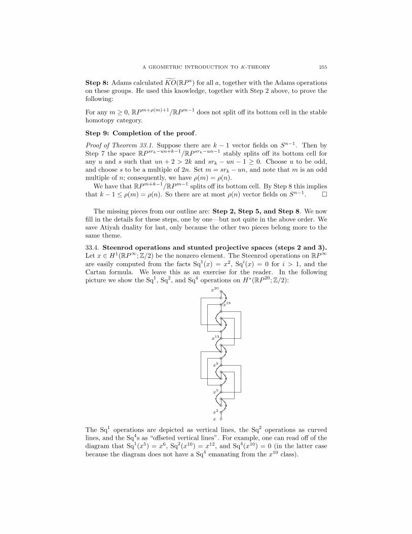
A GEOMETRIC INTRODUCTION TO K-THEORY 255
Step 8: Adams calculated KO(RP a) for all a, together with the Adams operationson these groups. He used this knowledge, together with Step 2 above, to prove thefollowing:
For any m ≥ 0, RPm+ρ(m)+1/RPm−1 does not split off its bottom cell in the stablehomotopy category.
Step 9: Completion of the proof .
Proof of Theorem 33.1. Suppose there are k − 1 vector fields on Sn−1. Then byStep 7 the space RP srk−un+k−1/RP srk−un−1 stably splits off its bottom cell forany u and s such that un + 2 > 2k and srk − un − 1 ≥ 0. Choose u to be odd,and choose s to be a multiple of 2n. Set m = srk − un, and note that m is an oddmultiple of n; consequently, we have ρ(m) = ρ(n).
We have that RPm+k−1/RPm−1 splits off its bottom cell. By Step 8 this impliesthat k − 1 ≤ ρ(m) = ρ(n). So there are at most ρ(n) vector fields on Sn−1.
The missing pieces from our outline are: Step 2, Step 5, and Step 8. We nowfill in the details for these steps, one by one—but not quite in the above order. Wesave Atiyah duality for last, only because the other two pieces belong more to thesame theme.
33.4. Steenrod operations and stunted projective spaces (steps 2 and 3).Let x ∈ H1(RP∞; Z/2) be the nonzero element. The Steenrod operations on RP∞
are easily computed from the facts Sq1(x) = x2, Sqi(x) = 0 for i > 1, and theCartan formula. We leave this as an exercise for the reader. In the followingpicture we show the Sq1, Sq2, and Sq4 operations on H∗(RP 20; Z/2):
bbbbbbbbbbbbbbbbbbbb
x
x2
x5
x9
x13
x18
x20
The Sq1 operations are depicted as vertical lines, the Sq2 operations as curvedlines, and the Sq4s as “offseted vertical lines”. For example, one can read off of thediagram that Sq1(x5) = x6, Sq2(x10) = x12, and Sq4(x10) = 0 (in the latter casebecause the diagram does not have a Sq4 emanating from the x10 class).

256 DANIEL DUGGER
The pattern of Sq2r
operations in H∗(RP∞; Z/2) is very simple. The first Sq2r
operation occurs on x2r
and thereafter they follow the pattern of “2r on/2r off”.This is captured by the formula
Sq2r
(xa) =
xa+2r
if a ≥ 2r and a ≡ 2r, 2r + 1, . . . , 2r+1 − 1 mod 2r+1,0 otherwise.
Of course for H∗(RPn; Z/2) the formulas must be truncated to account for the factthat classes above dimension n are not present.
To see how Steenrod operations give obstructions to stable splittings, considerRP 9/RP 6. Its cohomology has a Sq2 connecting the class in degree 7 to the classin degree 9. Suppose the projection onto the top cell p : RP 9/RP 6 → S9 has asplitting χ in the stable homotopy category. Then the composite
H∗(S9)p∗−→ H∗(RP 9/RP 6)
χ∗−→ H∗(S9)
is an isomorphism. Write xi for the generator in Hi(RP 9/RP 6), so that in thisnotation we have Sq2(x7) = x9. Necessarily we must have χ∗(x7) = 0, therefore0 = Sq2(χ∗x7) = χ∗(Sq2 x7) = χ∗(x9). But x9 is in the image of p∗, so this is acontradiction.
Clearly this kind of argument will work for any RPn/RPn−b where we have anontrivial cohomology operation hitting the top class. Based on this, it is now easyto prove the following:
Proposition 33.5. Write n + 1 = 2s · odd. If RPn/RPn−b splits off its top cellstably then b ≤ 2s.
Proof. If n is even then in H∗(RP∞) there is a Sq1 hitting the class in degree n,and this operation will be present in H∗(RPn/RPn−b) as long as b > 1. So the topcell can not split off in this case. In other words, if n+ 1 = 20 · (odd) then splittingof the top cell can only happen if b ≤ 20.
Similarly, if n = 4e + 1 then in H∗(RP∞) there is a Sq2 hitting the class indegree n. This Sq2 will be present in H∗(RPn/RPn−b) as long as b > 2, and againwe find that under this criterion the top cell can not split off. So n+ 1 = 21 · (odd)implies splitting of the top cell can only happen if b ≤ 21.
The same style of argument continues. If n = 2re + (2r−1 − 1) then there is aSq2r−1
hitting our class in degree n, and this obstructs the splitting of the top cellas long as b > 2r−1. Rephrased, this says that if n + 1 = 2r−1(2e + 1) then thesplitting does not exist when b > 2r−1. Replacing r− 1 with s, we have the desiredresult.
Corollary 33.6. If n = 2s · odd then there are at most 2s − 1 independent vectorfields on Sn−1.
Proof. If there are k − 1 vector fields on Sn−1 then RPun−1/RPun−k−1 splits offits top cell for all u 0. Choose a u that is odd, so that un = 2s · odd. ByProposition 33.5 we conclude that k ≤ 2s.
The upper bounds provided by Corollary 33.6 agree with the Hurwitz-Radonlower bounds when s ≤ 3. Note that these few cases cover quite a bit more thanone first might think. For example, for spheres of dimension less than 50 it followsthat the Hurwitz-Radon number of vector fields is the maximum possible for all
A GEOMETRIC INTRODUCTION TO K-THEORY 257
but three cases, namely the spheres S15, S31, and S47 (multiples of 16 minus one).Corollary 33.6 yields that there exist at most 15 vector fields on S15, 31 on S31,and 15 on S47, whereas the Hurwitz-Radon construction only gives 8 vector fieldson S15 and S47, and 9 vector fields on S31. This demonstrates that our bounds forthe spheres S16e−1 are still far away from our goal.
33.7. Adams’s Theorem and KO-theory (Step 8). Next we move to the piecethat finally cracked the proof, namely the following theorem of Adams [Ad2]:
Theorem 33.8. Let m ≥ 1. Then the space RPm+ρ(m)+1/RPm−1 does not splitoff its bottom cell in the stable homotopy category.
Proof. Write m = 2u ·odd, and consider RPN/RPm−1 for N ≥ m. Note that thereis a Sq2u
operation on H∗(RPN/RPm−1; Z/2) connecting the generator in degreem to the generator in degree m + 2u. This proves that the bottom cell does notsplit off when N ≥ m + 2u. This settles the theorem in the case u ≤ 3, as hereρ(m) = 2u − 1 and so m+ 2u = m+ ρ(m) + 1.
We will next do a similar argument—but using K-theory—in the case u ≥ 4.Actually, the K-theory argument only uses u ≥ 3 so for the sake of pedagogy letus just make this weaker assumption.
Since m ≡ 0 mod 4 we know by Theorem 32.18 that there is a short exactsequence(33.9)
0 KO (RPm/RPm−1)oo
∼=
KO (RPN/RPm−1)oo KO (RPN/RPm)oo
∼=
0oo
Z Z/(2f )
where f is a certain integer we will recall in a moment. Each of the groups hasAdams operations on it, and the maps are compatible with these operations. Ifwe let B = Z[ψ2, ψ3, ψ5, . . .], then (33.9) is an exact sequence of B-modules (notethat B is just the monoid ring Z[N] from Section 31). If RPN/RPm−1 splits off itsbottom cell then this extension is split; so we will attempt to algebraically analyzewhen such a splitting exists.
As a B-module the group KO (RPm/RPm−1) is Z(m2 ), meaning that each ψk
acts as multiplication by km2 . It will be convenient to set r = m
2 . Also, we know byTheorem 32.18(a) that on KO (RPN/RPm) the operation ψk acts as zero when kis even, and the identity when k is odd. We also have determined the action of theψk’s on the middle group, but let us ignore this for the moment and consider thesituation in a bit more generality.
Let A be any abelian group, and let A[2] be the B-module whose underlyingabelian group is A and where ψk acts as zero when k is even, and the identity whenk is odd. Consider an extension of B-modules
0← Z(r)← E ← A[2]← 0.
Let g be an element of E that maps onto a generator for Z(r). Then we can writeψkg = krg + αk for unique elements αk ∈ A, and the relations ψkψl = ψlψk show
258 DANIEL DUGGER
that we must havekrαl = (lr − 1)αk whenever k is even and l is odd,krαl = lrαk whenever k and l are both even,(kr − 1)αl = (lr − 1)αk whenever k and l are both odd.
(33.10)
So the extension E is determined by the elements αk ∈ A, for k ≥ 2, satisfying theabove equations.
To analyze when the sequence is split, let g denote the image of g in Z(r). Asplitting would send g to an element g + a, for some a ∈ A. Since ψk(g) = kr g wefind that
kr(g + a) = ψk(g + a) = krg + αk +
0 if k is even,a if k is odd.
Rearranging to solve for αk, we obtain
αk =
kra if k is even,(kr − 1)a if k is odd.
So these are the properties of an (αk) sequence that are equivalent to the extension0 ← Z(r) ← E ← A[2] ← 0 being split. Notice that such sequences are in somesense the “trivial” solutions of the relations (33.10).
We make one more general comment before returning to our specific situation.Let a ∈ A and consider the sequence defined by
αk =
12k
r.a k even12 (kr − 1).a k odd.
(33.11)
Note that the fractions multiplying a are in fact integers. So this sequence definesa valid extension E, and if a is not a multiple of 2 in A then the extension doesn’t“look” split. Precisely, if A is torsion-free and a /∈ 2A, then the extension is clearlynonsplit. We will see that the case where A is torsion is a bit more subtle.
Now let us return to the extension in (33.9). Here A = Z/(2f ), where f =ϕ(N) − ϕ(m). Since m is a multiple of 8 (and this is the first place where we usethis assumption), f also equals ϕ(N −m).
In Theorem 32.19 we previously computed the action of the Adams operationson KO (RPN/RPm−1). The corresponding α-sequence is precisely the one givenby (33.11), where a is a generator for Z/(2f ). So the extension is split if and onlyif there exists a B ∈ Z such that
12k
r.a = kr.(Ba) (k even), 12 (kr − 1).a = (kr − 1).(Ba) (k odd)
for all k. Phrased differently, these say that
2f divides
12k
r(1− 2B) if k is even,12 (kr − 1)(1− 2B) if k is odd.
Since 1− 2B is always odd, this is equivalent to
2f+1 divides
kr k even,kr − 1 k odd.
A GEOMETRIC INTRODUCTION TO K-THEORY 259
Let ν(x) denote the 2-adic valuation of the integer x, and let us restate what wehave now shown: If 8|m and RPN/RPm−1 splits off its bottom cell, then
ϕ(N −m) + 1 ≤ minr, ν(3r − 1), ν(5r − 1), ν(7r − 1), ν(9r − 1), . . .
where r = m/2. Here we have used ν(2r) = r and have also left out ν(kr) foreven integers k > 2, as these numbers are at least r and hence irrelevant for theminimum.
Our next task is to consider the numbers ν(3r − 1), and for these we refer toLemma 33.12 below. Since in our case r is even one has ν(3r − 1) = ν(r) + 2.Note that as r ≥ 4 this term is no larger than r, and so the first term in the aboveminimum is irrelevant.
We could proceed to analyze the terms ν(kr − 1) for odd k > 3, which is nothard, but in fact we have done enough to conclude the proof already. We haveshown that if 8|m and RPN/RPm−1 splits off its bottom cell, then
ϕ(N −m) + 1 ≤ ν(r) + 2 = ν(m) + 1,
or simply ϕ(N −m) ≤ ν(m). So our task is to find the largest x for which ϕ(x) =ν(m). To do this, write ν(m) = 4b + a where 0 ≤ a ≤ 3. Let “ϕ-count” stand forcounting the integers that are congruent to 0, 1, 2, or 4 modulo 8. Every cycle of8 consecutive integers contribules 4 to the ϕ-count, and so for ϕ(x) ≥ 4b we wouldneed x ≥ 8b. The cases a = 0, 1, 2, 3 can now be analyzed by hand: for a = 0 wehave x = 8b; for a = 1 we have x = 8b + 1; for a = 2 we have x = 8b + 3; and fora = 3 we have x = 8b + 7. So in general the largest x such that ϕ(x) = 4b + a isx = 8b+ 2a − 1.
Putting everything together, if ϕ(N − m) ≤ ν(m) = 4b + a then N − m ≤8b+ 2a− 1 = ρ(m). So if N ≥ m+ ρ(m) + 1 then RPN/RPm−1 cannot split off itsbottom cell.
Lemma 33.12. If r is even then ν(3r−1) = ν(r)+2. If r is odd then ν(3r−1) = 1.
Proof. If r is odd then modulo 4 we have 3r = (−1)r = −1, so 3r − 1 ≡ 2 mod 4.This proves that ν(3r − 1) = 1.
If r = 2f · u where u is odd, we prove by induction on f that ν(3r − 1) = f + 2.The base case is f = 1, and here we use 3r−1 = 32u−1 = (3u−1)(3u+1). We knowν(3u−1) = 1 by the preceding paragraph. Modulo 4 one has 3u+1 = (−1)u+1 = 0,but modulo 8 one has 3u+1 = 4. So ν(3u+1) = 2, which confirms that ν(3r−1) = 3.
For the inductive step, if r = 2f+1u where u is odd then write
3r − 1 = (32fu − 1)(32fu + 1).
By induction we know ν(32fu − 1) = f + 2. Modulo 4 we have 32fu + 1 =((−1)2
f )u+1 = 1 + 1 = 2. So ν(32fu + 1) = 1, hence ν(3r − 1) = f + 3.
Remark 33.13. It is intriguing that a number-theoretic analysis of ν(3r − 1) wasthe ultimate step in both the Hopf invariant one problem and the vector fields onspheres problem. To my knowledge, there is no reason to suspect any connectionbetween these two problems.
Exercise 33.14. If k is any odd number, prove that ν(kr − 1) ≥ ν(r) + 2 when ris even. This confirms that the terms for k > 3 were irrelevant for the minimumconsidered in the above proof.
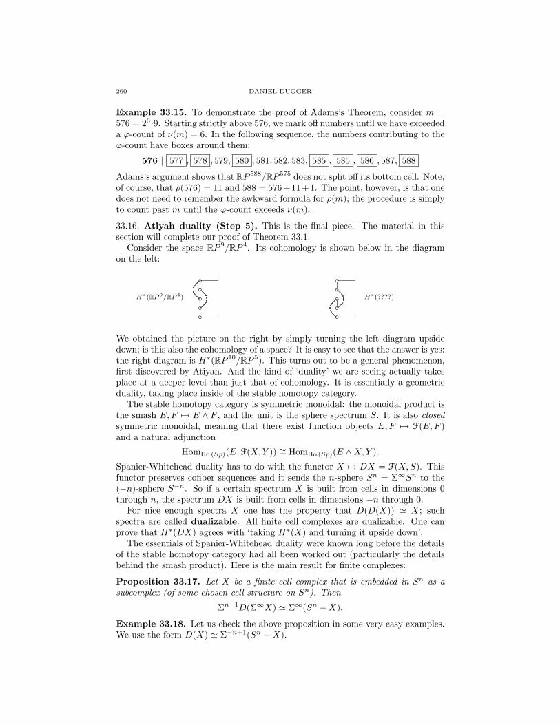
260 DANIEL DUGGER
Example 33.15. To demonstrate the proof of Adams’s Theorem, consider m =576 = 26·9. Starting strictly above 576, we mark off numbers until we have exceededa ϕ-count of ν(m) = 6. In the following sequence, the numbers contributing to theϕ-count have boxes around them:
576 | 577 , 578 , 579, 580 , 581, 582, 583, 585 , 585 , 586 , 587, 588
Adams’s argument shows that RP 588/RP 575 does not split off its bottom cell. Note,of course, that ρ(576) = 11 and 588 = 576+11+1. The point, however, is that onedoes not need to remember the awkward formula for ρ(m); the procedure is simplyto count past m until the ϕ-count exceeds ν(m).
33.16. Atiyah duality (Step 5). This is the final piece. The material in thissection will complete our proof of Theorem 33.1.
Consider the space RP 9/RP 4. Its cohomology is shown below in the diagramon the left:
bbbbb
H∗(RP 9/RP 4) bbbbb
H∗(????)
We obtained the picture on the right by simply turning the left diagram upsidedown; is this also the cohomology of a space? It is easy to see that the answer is yes:the right diagram is H∗(RP 10/RP 5). This turns out to be a general phenomenon,first discovered by Atiyah. And the kind of ‘duality’ we are seeing actually takesplace at a deeper level than just that of cohomology. It is essentially a geometricduality, taking place inside of the stable homotopy category.
The stable homotopy category is symmetric monoidal: the monoidal product isthe smash E,F 7→ E ∧ F , and the unit is the sphere spectrum S. It is also closedsymmetric monoidal, meaning that there exist function objects E,F 7→ F(E,F )and a natural adjunction
HomHo (Sp)(E,F(X,Y )) ∼= HomHo (Sp)(E ∧X,Y ).
Spanier-Whitehead duality has to do with the functor X 7→ DX = F(X,S). Thisfunctor preserves cofiber sequences and it sends the n-sphere Sn = Σ∞Sn to the(−n)-sphere S−n. So if a certain spectrum X is built from cells in dimensions 0through n, the spectrum DX is built from cells in dimensions −n through 0.
For nice enough spectra X one has the property that D(D(X)) ' X; suchspectra are called dualizable. All finite cell complexes are dualizable. One canprove that H∗(DX) agrees with ‘taking H∗(X) and turning it upside down’.
The essentials of Spanier-Whitehead duality were known long before the detailsof the stable homotopy category had all been worked out (particularly the detailsbehind the smash product). Here is the main result for finite complexes:
Proposition 33.17. Let X be a finite cell complex that is embedded in Sn as asubcomplex (of some chosen cell structure on Sn). Then
Σn−1D(Σ∞X) ' Σ∞(Sn −X).
Example 33.18. Let us check the above proposition in some very easy examples.We use the form D(X) ' Σ−n+1(Sn −X).
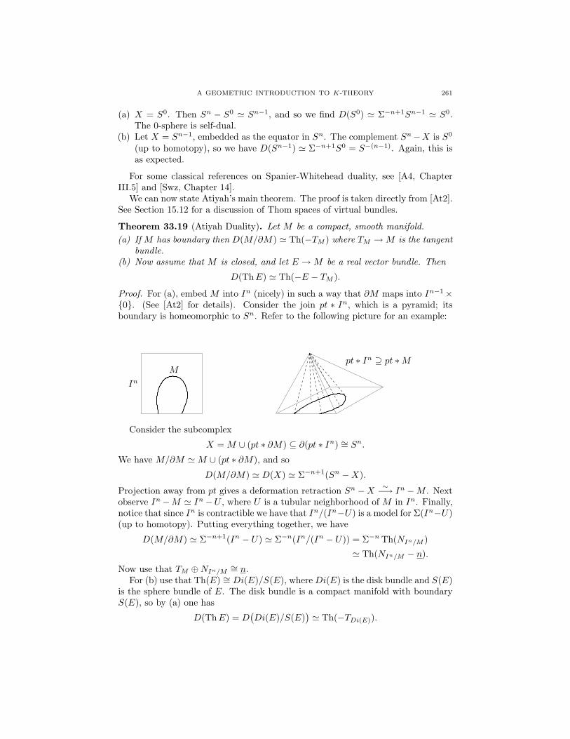
A GEOMETRIC INTRODUCTION TO K-THEORY 261
(a) X = S0. Then Sn − S0 ' Sn−1, and so we find D(S0) ' Σ−n+1Sn−1 ' S0.The 0-sphere is self-dual.
(b) Let X = Sn−1, embedded as the equator in Sn. The complement Sn−X is S0
(up to homotopy), so we have D(Sn−1) ' Σ−n+1S0 = S−(n−1). Again, this isas expected.
For some classical references on Spanier-Whitehead duality, see [A4, ChapterIII.5] and [Swz, Chapter 14].
We can now state Atiyah’s main theorem. The proof is taken directly from [At2].See Section 15.12 for a discussion of Thom spaces of virtual bundles.
Theorem 33.19 (Atiyah Duality). Let M be a compact, smooth manifold.(a) If M has boundary then D(M/∂M) ' Th(−TM ) where TM →M is the tangent
bundle.(b) Now assume that M is closed, and let E →M be a real vector bundle. Then
D(ThE) ' Th(−E − TM ).
Proof. For (a), embed M into In (nicely) in such a way that ∂M maps into In−1×0. (See [At2] for details). Consider the join pt ∗ In, which is a pyramid; itsboundary is homeomorphic to Sn. Refer to the following picture for an example:
InM
pt ∗ In ⊇ pt ∗M
Consider the subcomplex
X = M ∪ (pt ∗ ∂M) ⊆ ∂(pt ∗ In) ∼= Sn.
We have M/∂M 'M ∪ (pt ∗ ∂M), and so
D(M/∂M) ' D(X) ' Σ−n+1(Sn −X).
Projection away from pt gives a deformation retraction Sn −X ∼−→ In −M . Nextobserve In−M ' In−U , where U is a tubular neighborhood of M in In. Finally,notice that since In is contractible we have that In/(In−U) is a model for Σ(In−U)(up to homotopy). Putting everything together, we have
D(M/∂M) ' Σ−n+1(In − U) ' Σ−n(In/(In − U)) = Σ−n Th(NIn/M )
' Th(NIn/M − n).
Now use that TM ⊕NIn/M∼= n.
For (b) use that Th(E) ∼= Di(E)/S(E), whereDi(E) is the disk bundle and S(E)is the sphere bundle of E. The disk bundle is a compact manifold with boundaryS(E), so by (a) one has
D(ThE) = D(Di(E)/S(E)
)' Th(−TDi(E)).

262 DANIEL DUGGER
If π : Di(E)→M is the bundle map then it is easy to see that TDi(E)∼= π∗(E⊕TM ).
Since π is a homotopy equivalence,
Th(−TDi(E)) = Th(−π∗(E ⊕ TM )) ' Th(−(E ⊕ TM )).
This finishes the proof.
We next apply what we just learned to stunted projective spaces. Recall fromExample 15.9 that all stunted projective spaces are Thom spaces:
RPn−1/RPn−k−1 ∼= Th
((n−k)L↓
RPk−1
).
Recall as well that the tangent bundle to RP k−1 satisfies T ⊕ 1 ∼= kL (Exam-ple 23.10). Using these two facts, Atiyah Duality now gives that
D(RPn−1/RPn−k−1) ' Th
(−(n−k)L−T
↓RPk−1
)= Th
(−nL+1
↓RPk−1
)' Σ Th
(−nL↓
RPk−1
).
Let rk−1 be the additive order of [L] − 1 in KO(RP k−1). Then rk−1L ∼= rk−1
(stably), and hence for any s ∈ Z we have
Th
(−nL↓
RPk−1
)' Σ−srk−1 Th
(−nL+srk−1
↓RPk−1
)' Σ−srk−1 Th
(−nL+srk−1L
↓RPk−1
)
' Σ−srk−1 Th
((srk−1−n)L
↓RPk−1
)'Σ−srk−1
[RP srk−1−n+k−1/RP srk−1−n−1
].
In the last line we imagine s chosen to be large enough so that srk−1 − n− 1 ≥ 0.Putting everything together, we have proven the following:
Corollary 33.20. Let rk−1 be the additive order of [L]− 1 in KO(RP k−1). Thenthere is a stable homotopy equivalence
D(RPn−1/RPn−k−1) ' Σ1−srk−1
[RP srk−1−n+k−1/RP srk−1−n−1
]where s is any integer such that srk−1 − n− 1 ≥ 0.
Example 33.21. Let us consider the Spanier-Whitehead dual of RP 9/RP 4, as inthe beginning of this section. Relative to our above discussion, n = 10 and k = 5.By Theorem 32.14 we know KO(RP 4) ∼= Z/8, so the order of [L] − 1 is 8. Theabove corollary gives
D(RP 9/RP 4) ' Σ1−8s[RP 8s−6/RP 8s−11
]for any s where the right-hand-side makes sense. The smallest choice is s = 2,giving D(RP 9/RP 4) ' Σ−15(RP 10/RP 5).

A GEOMETRIC INTRODUCTION TO K-THEORY 263
34. The immersion problem for RPn
Let M be a compact, n-dimensional, real manifold. It is a classical theorem ofWhitney from the 1940s that M can be immersed in R2n−1 and embedded into R2n
[Wh1, Wh2]. A much more difficult result, proved by Cohen [C] in 1985, says thatM can be immersed in R2n−α(n) where α(n) is the number of ones in the binaryexpansion of n. As a general result this is known to be the best possible, butfor specific choices of M one could conceivably do better. Define the immersiondimension (resp. the embedding dimension) of M to be the smallest k suchthat M immerses (resp., embeds) into Rk.
In general, determining the immersion and embedding dimensions of a givenmanifold seem to be difficult problems. Over the last 60+ years they have beenextensively studied, particularly for the manifold RPn. The problem tends toinvolve two distinct components. As one aspect, clever geometric constructions areused to produce immersions (or embeddings) and therefore upper bounds on theimmersion dimension. For lower bounds one must prove non-immersion results, andthis is usually done by making use of some sort of homotopical invariants. Overthe years the problem for RPn has been used as a sort of testing ground for everynew homotopical technique to come along.
Our intent here is not to give a complete survey of this problem, as this wouldtake far too long. We will be content to give a small taste, entirely concentratingour focus on some easily-obtained lower bounds in the case of RPn. The methodsinvolve Stiefel-Whitney classes (in singular cohomology) and some related charac-teristic classes in KO-theory.
34.1. A short survey. Before jumping into our analysis, let us give some sense ofwhat is known about the problem. The following table shows the current knowledge(as of January 2013) about the immersion and embedding dimensions for RPn whenn ≤ 24:
Table 34.2. Immersion and embedding dimensions for RPn
RPn 2 3 4 5 6 7 8 9 10 11 12 13imm. dim. 3 4 7 7 7 8 15 15 16 16 18 22emb. dim. 4 5 8 9 [9, 11] [9, 12] 16 17 17 18 [18, 21] [22, 23]
RPn 14 15 16 17 18 19 20 21 22 23 24imm. 22 22 31 31 32 32 34 38 38 38 [38, 39]emb. [22, 23] [23, 24] 32 33 33 [33, 34] [34, 37] 39 39 39 [39, 42]
In the table, entries in brackets are given when the exact answer is not known.For example, the embedding dimension of RP 6 is only known to lie in the interval[9, 11]. RP 6 definitely embeds into R11 and does not embed into R8—but it is notknown if RP 6 embeds into R9 or R10. In comparison, we know much more aboutthe immersion problem; the smallest unknown case is RP 24.
The above data on the immersion and embedding dimensions was taken from atable compiled by Don Davis [Da]. Davis’s table contains substantially more data,covering slightly past RP 100.

264 DANIEL DUGGER
One of the earliest results is due to Milnor: if n = 2r then the immersiondimension of RPn equals 2n− 1 (showing that the Whitney upper bound is sharpin this case). Peterson proved that if n = 2r then the embedding dimension equals2n, again showing that the Whitney bound is sharp here. In general, if n = 2r + dfor 0 ≤ d < 2r and d is relatively small, then one can expect the immersion andembedding dimensions to be 2r+1 + x where x is a known quantity or one that istightly constrained. The following theorem encompasses most of what is known ford ≤ 10:
Theorem 34.3. Write n = 2i+d where 0 ≤ d < 2i. Then the immersion dimensionof RPn equals 2i+1 + e and the embedding dimension equals 2i+1 + f where thefollowing is known:
d 0 1 2 3 4 5 6 7 8 9 10i ≥ 1 ≥ 2 ≥ 3 ≥ 4 ≥ 4 ≥ 4 ≥ 4 ≥ 4 ≥ 4 ≥ 4 ≥ 4e −1 −1 0 0 2 6 6 6 [6, 7] 14 14f 0 1 1 [1, 2] [2, 5] 7 7 7 [7, 10] [14, 15] [14, 16]
The above theorem is not credited because it represents the combined work overmany years of a dozen authors. Much credit should be given to Davis, who hasbrought all the results together and given complete references. The above theoremis just the first few lines of the table [Da].
34.4. Stiefel-Whitney techniques. Suppose that M is a compact manifold ofdimension n, and that M is immersed in Rn+k. The immersion has a normalbundle ν, and there is an isomorphism of bundles TM ⊕ ν ∼= n+ k. Taking totalStiefel-Whitney classes of both sides gives
w(TM ) · w(ν) = w(TM ⊕ ν) = w(n+ k) = 1.
Recall that the total Stiefel-Whitney class of a bundle E is w(E) = 1 + w1(E) +w2(E)+· · · . Because the zero-coefficient is 1 we can formally invert this expression,and because H∗(M) is zero in sufficiently large degrees this formal inverse actuallymakes sense as an element of H∗(M). So we can feel free to write w(E)−1, and weobtain
w(TM )−1 = w(ν).We don’t know anything about ν except its rank, which is equal to k. This guar-antees that w(ν) does not have any terms of degree larger than k, and so we obtainthe following simple result [MS, material preceding Theorem 4.8]:
Proposition 34.5. Let M be a compact manifold of dimension n. If M immersesin Rn+k then w(TM )−1 vanishes in degrees larger than k.
Let us apply this proposition to RPn. Here we have the identity TRPn ⊕ 1 =(n+ 1)L (Example 23.10) and so
w(TRPn) = w(TRPn ⊕ 1) = w((n+ 1)L) = w(L)n+1 = (1 + x)n+1,
where x denotes the generator for H1(RPn; Z/2). Taking inverses gives
w(TRPn)−1 = (1 + x)−(n+1) =∞∑i=0
(−(n+1)i
)xi.
A GEOMETRIC INTRODUCTION TO K-THEORY 265
We can rewrite the coefficient of xi, since(−(n+1)i
)= (−1)i (n+1)·(n+2)···(n+i)
i! = (−1)i(n+ii
).
Putting everything together we obtain the following:
Corollary 34.6. If RPn immerses into Rn+k then(n+ii
)is even for k < i ≤ n.
The above corollary yields very concrete non-immersion results, but to obtainthese we need to be good at checking when binomial coefficients are even. His-torically, topologists got pretty good at this because of the presence of binomialcoefficients in the Adem relations. The important result is the following:
Lemma 34.7. Let njnj−1 . . . n0 be the base 2 representation for n; that is, eachnj ∈ 0, 1 and n =
∑nj2j. Similarly, let kjkj−1 . . . k0 be the base 2 representation
for k. Then (nk
)≡∏i
(ni
ki
)mod 2.
Proof. The result follows easily from three points: (i)(2ni
)is even if i is odd; (ii)(
2n2k
)≡(nk
)(mod 2); and (iii)
(2n+12k
)≡(2n2k
)(mod 2). For (i) and (ii), imagine a
column of the numbers 1 through n and a second “mirror” column containing thesame entries. If i is odd, the i-element subsets of the two columns together maybe partitioned into two classes: those which contain more elements from columnA than column B, and those which contain less elements from column A. Theoperation of “switch entries between the two columns” gives a bijection betweenthese two classes, thereby showing that
(2ni
)is even.
For (ii), note that the i-element subsets can be partitioned into groups deter-mined by the number of elements from column A. This gives rise to the formula(
2n2k
)=(n0
)(nk
)+(n1
)(nk−1
)+ · · ·+
(nk−1
)(n1
)+(nk
)(n0
).
The terms on the right-hand-side are symmetric and so can be grouped in pairs,except for the middle term which is
(nk
)2. So working mod 2 we have(2n2k
)≡(nk
)2 ≡ (nk).For (iii) just use Pascal’s identity
(2n+12k
)=(2n2k
)+(
2n2k−1
)together with (i).
Example 34.8. To determine if(209
)is even then we note that 20 is 10100 in base
2, and 9 is 1001. Using the above lemma we compute(209
)=(
1 0 1 0 00 1 0 0 1
)≡(10
)(01
)(10
)(00
)(01
)= 1 · 0 · 1 · 1 · 0 = 0.
So(209
)is even.
Notice that(11
)=(10
)=(00
)= 1, whereas
(01
)= 0. So in computations like the
one above, the fnal answer is even if and only if(01
)appears at least once in the
product—that is, if n has a certain bit turned “off” and the corresponding bit of kis “on”. In particular, the following three statements are now obvious:
(i) If n = 2r then(ni
)is even for all i in the range 0 < i < n.
(ii) If n = 2r − 1 then(ni
)is odd for all i ≤ n.
(iii)(2nn
)is always even.
The point for the first two is that 2r has all of its bits turned off except for therth, whereas 2r−1 has all of its bits turned on. For statement (iii) just consider thesmallest bit of n that is turned on, and note that the corresponding bit is off in 2n.

266 DANIEL DUGGER
Corollary 34.6 is most often used in the form below. The proof is immediatefrom Corollary 34.6.
Corollary 34.9. Fix n ≥ 2, and let k be the largest integer such that k ≤ n and(n+kk
)is odd. Then RPn does not immerse into Rn+k−1.
Note that k will be strictly less than n, as(2nn
)is always even; this conforms with
the Whitney immersion result. As an application of the above corollary, supposewe want to immerse RP 10. We start with(
2010
)= 20·19·18·17·16·15·14·13·12·11
10·9·8·7·6·5·4·3·2·1
We have 210 dividing the numerator and 28 dividing the denominator. Start re-moving factors from the left, one by one from the numerator and denominatorsimultaneously, watching what happens to the number of 2’s in each. The fractiondoes not become odd until we are looking at
(155
). So the conclusion is that RP 10
does not immerse into RP 14.The above process is cumbersome, and with a little investigation it is not hard
to produce a shortcut.
Proposition 34.10. Write n = 2i + d where 0 ≤ d < 2i. Then the largest k in therange 0 ≤ k ≤ n such that
(n+kk
)is odd is k = 2i − d− 1.
Proof. Note that if j = 2i−d−1 then n+j = 2i+1−1 and so(n+jj
)is certainly odd.
We must show that(n+jj
)is even for j in the range 2i−d ≤ j ≤ n. This is the kind
of analysis that is perhaps best left to the reader, but we will give a sketch. Supposeto the contrary that j is in this range and
(n+jj
)is odd. Let e = j − (2i − d − 1),
so that n + j = (2i + d) + e + (2i − d − 1) = e + (2i+1 − 1). Let the smallest bitof e that is turned on be the rth bit; this is also the smallest bit of n + j that isturned off. Since
(n+jn
)is odd, this bit must be also off in n. If we write e = e′+2r,
then n+ j = e′ + (2r + 2i+1 − 1). The term in parentheses has all bits off from the(r + 1)st through the ith, and so the bits of n+ j agree with the bits of e′ (and ofe) in this range. Since
(n+jn
)is odd, every bit of n that is turned on in this range
must also be turned on in n+ j—and therefore also in e. We have thus shown that• The rth bit is off in n but on in e, and• All bits greater than the rth that are on in n are also on in e.
These two facts show that e > n, which is not allowed since e ≤ j ≤ n.
Corollary 34.11. If n = 2i + d where 0 ≤ d ≤ 2i − 1 then RPn does not immerseinto R2i+1−2. In particular, if n = 2i then the immersion dimension of RPn equals2n− 1.
Proof. The first line is immediate from Corollary 34.9 and Proposition 34.10. Thesecond statement follows from the first together with the Whitney theorem sayingthat RPn immerses into R2n−1.
Let us now change gears just a bit and consider embeddings. We can also usecharacteristic classes to give obstructions in this setting. The key result is thefollowing:
Proposition 34.12. Suppose M is a compact n-manifold that is embedded in Rn+k.Then wk(ν) = 0 where ν is the normal bundle.

A GEOMETRIC INTRODUCTION TO K-THEORY 267
Proof. Choose a metric on ν and let S(ν) be the sphere bundle. If p : S(ν) → Mdenotes the projection map, then clearly p∗ν splits off a trivial bundle: p∗ν = 1⊕Efor some rank k − 1 bundle E on S(ν). From this it immediately follows that0 = wk(p∗ν) = p∗(wk(ν)).
The proof will be completed by showing that p∗ : H∗(M ; Z/2)→ H∗(S(ν); Z/2)is injective. Let U be a tubular neighborhood of M in Rn+k, arranged so that itsclosure U is homeomorphic to the disk bundle of ν. Write ∂U for the boundary,which is isomorphic to S(ν). We have the long exact sequence
· · · → Hi(U, ∂U)→ Hi(U)→ Hi(∂U)→ · · ·where all cohomology groups have Z/2-coefficients. The projection U → M is ahomotopy equivalence, so our map p∗ is isomorphic to Hi(U) → Hi(∂U). We canverify that this is injective by checking that the previous map in the long exactsequence is zero. We look only at i > 0, as the i = 0 case is trivial.
To this end, consider the diagram below:
Hi(Rn+k,Rn+k −M) //
∼=
Hi(Rn+k)
Hi(U, ∂U) // Hi(U)
The left vertical map is an isomorphism by excision, and the group in the upperright corner is zero. So the bottom horizontal map is zero, as we desired.
Compare the next result to Proposition 34.5:
Corollary 34.13. Let M be a compact n-manifold. If M embeds into Rn+k thenw(TM )−1 vanishes in degrees k and larger.
Proof. We saw in the proof of Proposition 34.5 that w(TM )−1 = w(ν). Since ν hasrank k, this forced the Stiefel-Whitney classes to vanish in degrees larger than k.But now Proposition 34.12 also gives us the vanishing in degree k.
Corollary 34.14. If RPn embeds into Rn+k then(n+jj
)is even for k ≤ j ≤ n.
Proof. Same as for Corollary 34.6.
Corollary 34.15. Let n = 2i+d where 0 ≤ d ≤ 2i− 1. Then RPn does not embedinto R2i+1−1. In particular, if n = 2i then the embedding dimension of RPn equals2n.
Proof. Let k be the largest integer in the range 0 ≤ k ≤ n such that(n+kk
)is
odd. Then Corollary 34.14 shows that RPn does not embed into Rn+k. ButProposition 34.10 identifies k = 2i−d−1, and so n+k = 2i+1−1. This proves thefirst statement. The second statement is then a consequence of the first togetherwith the Whitney theorem that RPn embeds into R2n.
To gauge the relative strength of Corollaries 34.11 and 34.15, see the table belowand compare to Table 34.2. One gets a clear sense of how far algebraic topologyhas progressed since the early days of Stiefel-Whitney classes!

268 DANIEL DUGGER
Table 34.16. Stiefel-Whitney lower bounds for the immersionand embedding dimensions of RPn
n 2 3 4 5 6 7 8 9 10 11 12 13 14 15 16 17 18imm≥ 3 3 7 7 7 7 15 15 15 15 15 15 15 15 15 15 15emb≥ 4 4 8 8 8 8 16 16 16 16 16 16 16 16 16 16 16
34.17. K-theoretic techniques. One can readily imagine taking the basic ap-proach from the last section and replacing the Stiefel-Whitney classes with charac-teristic classes taking values in some other cohomology theory. Atiyah [At3] pursuedthis idea using KO-theory, and certain constructions of Grothendieck provided theappropriate theory of characteristic classes. In this way he obtained some newnon-immersion and non-embedding theorems. We describe this work next.
Earlier in these notes (????) we described the construction of the γ-operations incomplex K-theory. The same formulas work just as well for KO-theory. Explicitly,for an element x ∈ KO (X) define
γt(x) = λ t1−t
(x) = 1 + t1−t [λ
1x] +(
t1−t)2[λ2x] + · · ·
Note that γt(x + y) = γt(x)γt(y). Define γi(x) to be the coefficient of ti in γt(x).So we have
γk(x+ y) =∑i+j=k
γi(x)γj(y).
Note also that γt(1) = 1 + t1−t = 1
1−t = 1 + t+ t2 + · · ·For a vector bundle E over X define
γt(E) = γt(E − rankE) =γt(E)
γt(rankE)=
γt(E)γt(1)rankE
= γt(E) · (1− t)rankE .
One should think of this as just being a renormalization of the γt construction; notethat γt(E) = 1 if E is a trivial bundle. Observe that we still have the analog of theWhitney formula:
γt(E ⊕ F ) = γt(E ⊕ F − rank(E + F )) = γt((E − rankE) + (F − rankF )
)= γt(E − rankE)γt(F − rankF )
= γt(E)γt(F ).
If L is a line bundle then
γt(L) = γt(L) · (1− t) =[1 + t
1−t [L]]· (1− t) = 1− t+ t[L] = 1 + t([L]− 1).
So γ1(L) = [L]− 1 and γi(L) = 0 for i > 1.Finally, we observe that if E is a rank k bundle then γi(E) = 0 for all i > k.
This is because
γt(E) = λ t1−t
(E)(1− t)k =∞∑i=0
( t1−t )
i[ΛiE] · (1− t)k =k∑i=0
ti(1− t)k−i[ΛiE].
Clearly the final expression is a polynomial in t of degree at most k.Compare the following result to Proposition 34.5 and Corollary 34.13.
Proposition 34.18. Let M be a compact n-manifold. If M immerses into Rn+k
then the power series γt(TM )−1 vanishes in degrees larger than k. If M embeds intoRn+k then γt(TM )−1 vanishes in degrees k and larger.

A GEOMETRIC INTRODUCTION TO K-THEORY 269
Proof. The proofs are the same as before. If M immerses into Rn+k then TM ⊕ν ∼=n+ k where ν is the normal bundle. So γt(TM )γt(ν) = γt(TM⊕ν) = γt(n+ k) = 1,and so γt(TM )−1 = γt(ν). But since ν has rank k we have γi(ν) = 0 for i > k.
For the second part of the proposition we need to prove that if M embeds intoRn+k then γk(ν) = 0. The proof is exactly the same as for Proposition 34.12.
For the following proposition, recall that ϕ(n) denotes the number of integers ssuch that 0 < s ≤ n and s is congruent to 0, 1, 2, or 4 modulo 8.
Corollary 34.19 (Atiyah).(a) If RPn immerses into Rn+k then 2ϕ(n)−j+1 divides
(n+jj
)for k < j ≤ ϕ(n).
(b) If RPn embeds into Rn+k then 2ϕ(n)−j+1 divides(n+jj
)for k ≤ j ≤ ϕ(n).
Proof. Recall that 1⊕ TRPn ∼= (n+ 1)L, as in Example 23.10. We get
γt(TRPn) = γt(TRPn ⊕ 1) = γt((n+ 1)L) = γt(L)n+1 =(1 + tλ
)n+1
where λ = [L]− 1 ∈ KO 0(RPn). So
γt(TRPn)−1 = (1 + tλ)−(n+1) =∞∑j=0
(−(n+1)j
)λj · tj =
∞∑j=0
(−1)j(n+jj
)λj · tj .
If RPn immerses into Rn+k then by Proposition 34.18(n+jj
)λj = 0 in KO 0(RPn)
for all k < j. If RPn embeds into Rn+k then(n+jj
)λj = 0 for all k ≤ j.
Now we recall from Theorem 32.14 that KO 0(RPn) ∼= Z/(2ϕ(n)) and that λ is agenerator. Also recall that λ2 = −2λ, or λj = (−2)j−1λ. The desired conclusionsfollow immediately.
Corollary 34.19 is best used in the following form. Let σ(n) denote the largestvalue of j in the range 1 ≤ j ≤ ϕ(n) for which
(n+jj
)is not divisible by 2ϕ(n)+1−j ;
if no such j exists then set σ(n) = 0 by default. Then RPn does not immerse intoRn+σ(n)−1 and does not embed into Rn+σ(n).
For some values of n the result of Corollary 34.19 is stronger than what weobtained from Corollaries 34.6 and 34.15, and for some values of n it is weaker. Wedemonstrate some examples:
Example 34.20. For the question of immersions of RP 8, we have ϕ(8) = 4 andσ(8) = 4. So Atiyah’s result (34.19) gives that RP 8 does not immerse into R11.The Stiefel-Whitney classes, however, told us that RP 8 does not immerse into R14.
In contrast, for RP 15 we have ϕ(15) = 7 and σ(15) = 4. So Atiyah’s result tellsus that RP 15 does not immerse into R18. The method of Stiefel-Whitney classes(34.6) gives no information in this case.
The table below shows the lower bounds for the immersion dimension of RPnobtained from Stiefel-Whitney techniques versus the KO-theoretic techniques. Thereader will notice that the Stiefel-Whitney bounds are significantly better whenn = 2i+d and d is small, whereas the KO-theoretic bounds are better for n = 2i+dwhen d is close to (but not exceeding) 2i − 1.
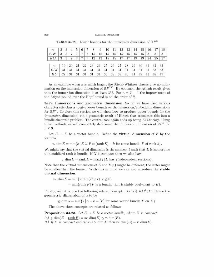
270 DANIEL DUGGER
Table 34.21. Lower bounds for the immersion dimension of RPn
n 2 3 4 5 6 7 8 9 10 11 12 13 14 15 16 17 18S-W 3 3 7 7 7 7 15 15 15 15 15 15 15 15 31 31 31KO 3 3 7 7 7 7 12 13 15 15 17 17 19 19 24 25 27
n 19 20 21 22 23 24 25 26 27 28 29 30 31 32 33S-W 31 31 31 31 31 31 31 31 31 31 31 31 31 63 63KO 27 31 31 31 31 34 35 38 39 40 41 42 43 48 49
As an example when n is much larger, the Stiefel-Whitney classes give no infor-mation on the immersion dimension of RP 255. By contrast, the Atiyah result givesthat the immersion dimension is at least 355. For n = 2i − 1 the improvement ofthe Atiyah bound over the Hopf bound is on the order of n
2 .
34.22. Immersions and geometric dimension. So far we have used variouscharacteristic classes to give lower bounds on the immersion/embedding dimensionsfor RPn. To close this section we will show how to produce upper bounds for theimmersion dimension, via a geometric result of Hirsch that translates this into abundle-theoretic problem. The central tool again ends up being KO-theory. Usingthese methods we will completely determine the immersion dimension of RPn forn ≤ 9.
Let E → X be a vector bundle. Define the virtual dimension of E by theformula
v.dimE = mink |E ∼= F ⊕ (rankE)− k for some bundle F of rank k.We might say that the virtual dimension is the smallest k such that E is isomorphicto a stablized rank k bundle. If X is compact then we also have
v.dimE = rankE −maxj |E has j independent sections.Note that the virtual dimensions of E and E⊕1 might be different; the latter mightbe smaller than the former. With this in mind we can also introduce the stablevirtual dimension:
sv.dimE = minv.dim(E ⊕ r) | r ≥ 0= minrankF |F is a bundle that is stably equivalent to E.
Finally, we introduce the following related concept. For α ∈ KO 0(X), define thegeometric dimension of α to be
g.dimα = mink∣∣α+ k = [F ] for some vector bundle F on X.
The above three concepts are related as follows:
Proposition 34.23. Let E → X be a vector bundle, where X is compact.(a) g.dim(E − rankE) = sv.dim(E) ≤ v.dim(E).(b) If X is compact and rankE > dimX then sv.dim(E) = v.dim(E).

A GEOMETRIC INTRODUCTION TO K-THEORY 271
Proof. For (a) only the first equality requires proof. This equality is almost atautology: for any integer d ≥ 0 we have
sv.dim(E) ≤ d ⇐⇒ there exists an F of rank d such that E ∼=st F
⇐⇒ there exists an F of rank d such that [E]− rankE = [F ]− d⇐⇒ there exists a bundle F such that [E]− rankE + d = [F ]
⇐⇒ g.dim(E − rankE) ≤ d.The desired equality follows immediately.
For (b), let r = sv.dim(E), k = rank(E), and note that r ≤ k. Then thereexists a rank r bundle F such that E and F are stably isomorphic: E ⊕ N ∼=F ⊕ (N + k − r) for some N > 0. Since rank(E) > dimX we can cancel the Nfactors to get E ∼= F⊕(k − r), by Proposition 11.10. Hence v.dim(E) ≤ rank(F ) =r = sv.dim(E).
The following result of Hirsch [Hi], and its corollary, translate the immersionproblem into a purely homotopy-theoretic question. This is the key to why immer-sions are better understood than embeddings.
Theorem 34.24 (Hirsch). Let M be a compact manifold of dimension n. Fork ≥ 1 the following statements are equivalent:(a) M can be immersed in Rn+k
(b) There exists a bundle F of rank k such that TM ⊕ F is trivial.(c) There exists an On-equivariant map Fr(TM )→ Vn(Rn+k), where Fr(TM ) is the
bundle of n-frames in TM .
Observe that (a) implies (b) by taking F to be the normal bundle of the im-mersion. Also, if φ : TM ⊕ F → n+ k is an isomorphism then any n-frame inTM yields an n-frame in Rn+k by applying φ; thus, one gets an equivariant mapFr(TM )→ Vn(Rn+k). This shows (b) implies (c). So the content of the above theo-rem is really in (c)⇒(a); this is what was proven by Hirsch, via geometric arguments[Hi, Theorem 6.1 (taking r = 0 there)]. He actually showed much more, essentiallyproving that homotopy classes of immersions from M to Rn+k are in bijective cor-respondence with equivariant homotopy classes of maps Fr(TM )→ Vn(Rn+k). Wewill not give Hirsch’s proof here, but we will use the following corollary of his result.This corollary first appeared in [At3, Proposition 3.2] and in [Sa1, Theorem 2.1].
Corollary 34.25. Let k ≥ 1, and let M be a compact manifold of dimension n.Then M immerses in Rn+k if and only if g.dim(n− TM ) ≤ k.
Proof. We have already seen the ‘only if’ direction when we obtained obstructionsto immersions: if an immersion exists then n+ k ∼= TM ⊕ ν where ν is the normalbundle, therefore n− TM = ν − k and hence g.dim(n− TM ) = g.dim(ν − k) ≤ k.
For the other direction, assume g.dim(n − TM ) ≤ k. So there exists a rank kvector bundle F such that n−TM +k = F in KO(M). This implies n+k = TM +Fin KO(M), which in turn yields that n+ k +N ∼= TM ⊕ F ⊕ N for some N ≥ 0.Since the rank of TM ⊕F is larger than dimM , it follows by Proposition 11.10 thatwe can cancel the N on both sides to get n+ k ∼= TM ⊕F . Then by Theorem 34.24we know that M immerses into Rn+k.
Remark 34.26. Note in particular that if M is parallelizable then M immersesinto Rn+1 (taking k = 1 in Corollary 34.25, since k = 0 is not allowed).
272 DANIEL DUGGER
We now specialize again to the case of M = RPn. Here we have
n− TRPn = (n+ 1)− (1⊕ TRPn) = (n+ 1)− (n+ 1)L = (n+ 1)(1− L).
Proposition 34.27. For n ≤ 8 the immersion dimension of RPn is as given inTable 34.2.
Proof. Given the lower bounds given by Stiefel-Whitney classes (see Table 34.21),we only have to demonstrate the required immersions. The fact that RP 8 immersesin R15 is a special case of Whitney’s classical theorem. Both RP 3 and RP 7 havetrivial tangent bundles, and so by Remark 34.26 they immerse into R4 and R8,respectively.
For RP 6 we must calculate the geometric dimension of 7(1−L) = −7(L−1). Butϕ(6) = 3, and so KO (RP 6) ∼= Z/8. Hence 8(L− 1) = 0, and so −7(L− 1) = L− 1.The geometric dimension of L − 1 is clearly at most 1, and so by Corollary 34.25RP 6 immerses into R7.
A similar argument works to show that RP 2 immerses into R3 (or one can justconstruct the immersion geometrically).
The reader should note why the above result stopped with RP 8. For RP 9
one finds that the immersion problem boils down to determining the geomet-ric dimension of −10(L − 1) = 22(L − 1) (here we used that ϕ(9) = 5 and soKO 0(RP 9) = Z/32). The precise value of this geometric dimension is far fromclear. We will close this section by analyzing it completely, following Sanderson[Sa1]. However, we take a short detour to illustrate some general principles.
Recall that for general n we have n− TRPn = (n+ 1)(1− L). We would like tointerpret the geometric dimension of this class as being a stable virtual dimension,but for this we would need to be looking at a positive multiple of L− 1 rather than1− L. There are two ways to get ourselves into this position. The first, which wehave already seen, proceeds by recalling that L − 1 has order 2ϕ(n) in KO (RPn).So we can write
n− TRPn = −(n+ 1)(L− 1) =(2ϕ(n) − (n+ 1)
)(L− 1)
and hence
g.dim(n− TRPn) = g.dim([
2ϕ(n) − (n+ 1)]L−
[2ϕ(n) − (n+ 1)
])= sv.dim
([2ϕ(n) − (n+ 1)
]L).
The second approach is from Sanderson [Sa2, Lemma 2.2]:
Proposition 34.28. For the bundle L→ RPn, the statement g.dim(a(L−1)) ≤ bis equivalent to g.dim((b− a)(L− 1)) ≤ b, for any a, b ∈ Z with b ≥ 0.
Proof. It suffices to prove the implication in one direction, by symmetry. So supposeg.dim(a(L− 1)) ≤ b. This implies that a(L− 1) + b = E in KO0(RPn), for somerank b bundle E. Multiply by L to get a(1−L) + bL = E ⊗L, and then rearrangeto find (b− a)(L− 1) + b = E ⊗L. This yields that g.dim((b− a)(L− 1)) ≤ b.
Corollary 34.29. Let L→ RPn be the tautological bundle. For k > 0 the followingstatements are equivalent:(1) RPn immerses into Rn+k,(2) g.dim(−(n+ 1)(L− 1)) ≤ k,
A GEOMETRIC INTRODUCTION TO K-THEORY 273
(3) g.dim((n+ k + 1)(L− 1)) ≤ k,(4) g.dim
([2ϕ(n) − (n+ 1)] (L− 1)
)≤ k.
Proof. The equivalence (1) ⇐⇒ (2) comes from Corollary 34.25, and (2) ⇐⇒ (3)is by Proposition 34.28. Finally, (2) ⇐⇒ (4) is true because 2ϕ(n)(L − 1) = 0 inKO 0(RPn).
Part (3) of the above result, which is the part that comes from Proposition 34.28,will not be needed in the remainder of this section. But we record it here for lateruse.
We close this section by settling the immersion problem for RP 9:
Proposition 34.30 (Sanderson). The immersion dimension of RP 9 equals 15.
This result is from [Sa1, Theorem 5.3]. Sanderson proves much more than this,for example that RPn immerses into R2n−3 whenever n is odd. He also proved thatRP 11 immerses into R16, which ends up being the best result for both RP 11 andRP 10.
Proof. The lower bound of 15 is given by Stiefel-Whitney classes, as in Table 34.21.So we only need to prove that RP 9 immerses into R15. By Corollary 34.29 this isequivalent to g.dim(22(L−1)) ≤ 6, and is also equivalent to g.dim(16(L−1)) ≤ 16.The proof below works for both statements, but for specificity we just prove theformer. Note that what we must prove is equivalent to sv.dim(22L) ≤ 6, byProposition 34.23. We will outline the steps for this, and then give more detailsafterwards.Step 1: There exists a rank 4 complex bundle E on RP 9 such that rRE is stablyequivalent to 22L (recall that rRE denotes the real bundle obtained from E byforgetting the complex structure).Step 2: The bundle E|RP 8 has a nonzero section s.Step 3: The bundle rRE|RP 8 has a field of (real) 2-frames.Step 4: For N 0 the field of real (2 + N)-frames of (rRE ⊕ N)|RP 8 may beextended over RP 9.Step 5: sv.dim(22L) = sv.dim(rRE) ≤ 6, hence RP 9 can be immersed into R15.
We now justify each of these steps. For step 1 use that rR : K(RPn) →KO (RPn) has image equal to 〈2(L − 1)〉, by Theorems 32.14 and 32.17. Since22 is even, there is a complex bundle E on RP 9 such that rRE is stably equivalentto 22L. The bundle E is represented by a map RP 9 → BU , and such a map nec-essarily factors up to homotopy through BU(4): for this, use obstruction theoryand the homotopy fiber sequences S2n−1 → BU(n − 1) → BU(n). For a mapRP 9 → BU(n) to lift (up to homotopy) into BU(n − 1), one has obstructions inthe groups Hi(RP 9;πi−1S
2n−1) for 0 ≤ i ≤ 9. But as long as 5 ≤ n the homotopygroups πi−1S
2n−1 vanish in this range, so all the obstruction groups are zero.For step 2 we again proceed by obstruction theory. We have the sphere bundle
S(E|RP 8) → RP 8 with fiber S7, and all the obstruction groups vanish except forthe last one: H8(RP 8;π7S
7). The coefficents are untwisted because the complexstructure gives a canonical orientation to each fiber. This final obstruction classis the same as the Euler class of rRE, or equivalently the top Chern class of E.Since H8(RP 8; Z) = Z/2 it will be sufficient to compute the mod 2 reduction ofthis class, which is the top Stiefel-Whitney class w8(rRE). Now we use that rRE isstably isomorphic to 22L, so the total Stiefel-Whitney class is w(rRE) = w(22L) =
274 DANIEL DUGGER
w(L)22 = (1 + x)22. Hence w8(rRE) =(228
)x8. Since
(228
)is even, the obstruction
class vanishes and we indeed have a nonzero section.Step 3 is trivial: the sections s and is give the field of real 2-frames.Step 4 is obstruction theory yet again. If F = rRE⊕N then we have a (partial)
section of VN+2(F ) → RP 9 defined over RP 8, and we must extend this to all ofRP 9. The obstruction lies in H9(RP 9;π8(VN+2(RN+8))). But the homotopy groupin the coefficients is known to be zero for large enough N , by ????.
Step 5 is now immediate: rRE ⊕N has rank 8 +N and has 2 +N independentsections, hence v.dim(rRE ⊕ N) ≤ 6. So sv.dim(rRE) ≤ 6 as well. Since rRE isstably equivalent to 22L, sv.dim(22L) = sv.dim(rRE) ≤ 6.
The arguments in this section naturally suggest the following problem, which isopen:
Problem: Given n and k, compute the geometric dimension of k([L] − 1) ∈KO (RPn).
Over the years this problem has been extensively studied by Adams, Davis, Gitler,Lam, Mahowald, Randall, and many others. See Section 35.14 for a bit morediscussion.
34.31. Summary. In this section we obtained two sets of non-immersion/non-embedding results, one using Stiefel-Whitney classes in mod 2 singular cohomologyand the other using the γ classes in KO-theory. We also translated the immersionproblem into a question about geometric dimension of reduced bundles, and forRPn we completely solved this question for n ≤ 9. As we have said before, this isfar from the whole story—in fact it is just the very tip of a large and interestingiceberg. We refer the reader to the references cited in [Da] for other pieces of thestory.
35. The sums-of-squares problem and beyond
This section is in some ways an epilogue to the previous one. In the last sectionwe started with a geometric problem, that of immersing RPn into Euclidean space.We then used cohomology theories and characteristic classes to obtain necessaryconditions for such an immersion to exist: we obtained two sets of conditions, onefrom mod 2 singular cohomology and one fromKO-theory. In the present section westart with an algebraic problem, one that at first glance seems completely unrelatedto immersions. It is the problem of finding sums-of-squares formulas in variousdimensions, which we encountered already back in Section 14 (we will review theproblem below). Once again we will use cohomology theories to obtain necessaryconditions for the existence of such formulas. The surprise is that these conditionsare basically the same as the ones that arose in the immersion problem! This isbecause both problems lead to the same homotopy-theoretic situation involvingbundles over real projective space.
In theory the present section could be read completely independently of the lastone. But because the underlying homotopy-theoretic problem is the same, we referto the previous section for many details of its analysis.
A GEOMETRIC INTRODUCTION TO K-THEORY 275
35.1. Review of the basic problem. Recall that a sums-of-squares formulaof type [r, s, n] (over R) is a bilinear map φ : Rr ⊗ Rs → Rn with the propertythat
|φ(x, y)|2 = |φ(x)|2 · |φ(y)|2(35.2)
for all x ∈ Rr and y ∈ Rs. If we write x = (x1, . . . , xr) and y = (y1, . . . , ys)then φ(x, y) = (z1, . . . , zn) where each zi is a bilinear expression in the x’s and y’s.Formula (35.2) becomes
(x21 + · · ·+ x2
r) · (y21 + · · ·+ y2
s) = z21 + · · ·+ z2
n.
We will sometimes refer to an “[r, s, n]-formula” for short. Note that if an [r, s, n]-formula exists then one trivially has [i, j, k]-formulas for any i ≤ r, j ≤ s, andk ≥ n.
For what values of r, s, and n does an [r, s, n]-formula exist? This is the sums-of-squares problem. Said differently, given a specific r and s what is the smallestvalue of n for which an [r, s, n]-formula exists? Call this number r ∗ s. As with theimmersion problem, there are two aspects here. One is the problem of constructingsums-of-squares formulas, thereby giving upper bounds for r ∗ s; the other is theproblem of finding necessary conditions for their existence, thereby giving lowerbounds. The latter is the part that involves topology.
The sums-of-squares formulas that everyone knows are the ones coming from themultiplications on R, C, H, and O. These haves types [1, 1, 1], [2, 2, 2], [4, 4, 4], and[8, 8, 8]. Hurwitz proved than an [n, n, n] formula only exists when n ∈ 1, 2, 4, 8,and the Hurwitz-Radon theorem generalizes this:
Theorem 35.3 (Hurwitz-Radon). A sums-of-squares formula of type [r, n, n] existsif and only if r ≤ ρ(n) + 1.
Proof. Write n = (odd) · 2a+4b with 0 ≤ a ≤ 3. Recall from Theorem 14.12 thatan [r, n, n]-formula exists if and only if there exists a Clr−1-module structure onRn. We saw in Section 14 that representations of Clr−1 only exist on vector spaceswhose dimension is a multiple of 2ϕ(r−1). Thus, we have the chain of equivalences
an [r, n, n]-formula exists ⇐⇒ there exists a Clr−1-module structure on Rn
⇐⇒ 2ϕ(r−1)∣∣n
⇐⇒ ϕ(r − 1) ≤ a+ 4b
⇐⇒ r − 1 ≤ 2a + 8b− 1 = ρ(n).
For the last equivalence note that ϕ(2a + 8b− 1) = ϕ(2a − 1) + 4b = a+ 4b, wherethe first equality is the 8-fold periodicity of ϕ and the second is just a calculationfor 0 ≤ a ≤ 3. Moreover, 2a + 8b− 1 is the largest number whose ϕ-value is a+ 4b;by periodicity this can again be checked just for b = 0 and 0 ≤ a ≤ 3. So in generalwe have ϕ(s) ≤ a+ 4b = ϕ(2a + 8b− 1) if and only if s ≤ 2a + 8b− 1; this is whatis used in the final equivalence.
Remark 35.4. Note that if there exist formulas of type [r, s1, n1] and [r, s2, n2]then there is also a formula of type [r, s1 + s2, n1 + n2] (by distribuitivity). Thissays that
r ∗ (s1 + s2) ≤ r ∗ s1 + r ∗ s2.
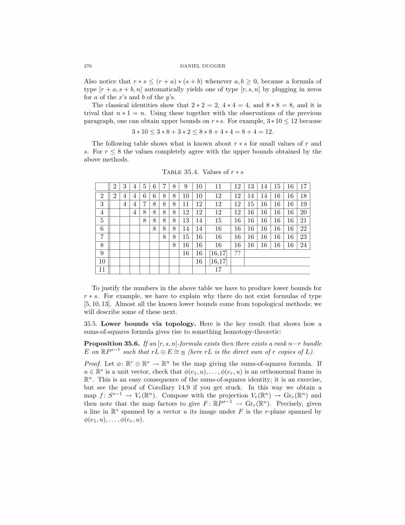
276 DANIEL DUGGER
Also notice that r ∗ s ≤ (r + a) ∗ (s + b) whenever a, b ≥ 0, because a formula oftype [r + a, s + b, n] automatically yields one of type [r, s, n] by plugging in zerosfor a of the x’s and b of the y’s.
The classical identities show that 2 ∗ 2 = 2, 4 ∗ 4 = 4, and 8 ∗ 8 = 8, and it istrival that n ∗ 1 = n. Using these together with the observations of the previousparagraph, one can obtain upper bounds on r ∗ s. For example, 3∗10 ≤ 12 because
3 ∗ 10 ≤ 3 ∗ 8 + 3 ∗ 2 ≤ 8 ∗ 8 + 4 ∗ 4 = 8 + 4 = 12.
The following table shows what is known about r ∗ s for small values of r ands. For r ≤ 8 the values completely agree with the upper bounds obtained by theabove methods.
Table 35.4. Values of r ∗ s
2 3 4 5 6 7 8 9 10 11 12 13 14 15 16 172 2 4 4 6 6 8 8 10 10 12 12 14 14 16 16 183 4 4 7 8 8 8 11 12 12 12 15 16 16 16 194 4 8 8 8 8 12 12 12 12 16 16 16 16 205 8 8 8 8 13 14 15 16 16 16 16 16 216 8 8 8 14 14 16 16 16 16 16 16 227 8 8 15 16 16 16 16 16 16 16 238 8 16 16 16 16 16 16 16 16 249 16 16 [16,17] ??10 16 [16,17]11 17
To justify the numbers in the above table we have to produce lower bounds forr ∗ s. For example, we have to explain why there do not exist formulas of type[5, 10, 13]. Almost all the known lower bounds come from topological methods; wewill describe some of these next.
35.5. Lower bounds via topology. Here is the key result that shows how asums-of-squares formula gives rise to something homotopy-theoretic:
Proposition 35.6. If an [r, s, n]-formula exists then there exists a rank n−r bundleE on RP s−1 such that rL⊕ E ∼= n (here rL is the direct sum of r copies of L).
Proof. Let φ : Rr ⊗ Rs → Rn be the map giving the sums-of-squares formula. Ifu ∈ Rs is a unit vector, check that φ(e1, u), . . . , φ(er, u) is an orthonormal frame inRn. This is an easy consequence of the sums-of-squares identity; it is an exercise,but see the proof of Corollary 14.9 if you get stuck. In this way we obtain amap f : Ss−1 → Vr(Rn). Compose with the projection Vr(Rn) → Grr(Rn) andthen note that the map factors to give F : RP s−1 → Grr(Rn). Precisely, givena line in Rs spanned by a vector u its image under F is the r-plane spanned byφ(e1, u), . . . , φ(er, u).
A GEOMETRIC INTRODUCTION TO K-THEORY 277
Let η be the tautological r-plane bundle on Grr(Rn). We claim that F ∗η = rL.This follows from the commutative diagram
rL
F // η
RP s−1 F // Grr(Rn)
where the top map is described as follows. Given r points on the same line 〈u〉 wewrite them as λ1u, . . . , λru and then send them to the element λ1φ(e1, u) + · · · +λrφ(er, u) on the r-plane F (〈u〉). One readily checks that this does not dependon the choice of u; in fact, we could just say that points z1, . . . , zr on a commonline ` are sent to the element φ(e1, z1) + · · · + φ(er, zr) on F (`). The fact thatφ(e1, u), . . . , φ(er, u) are orthonormal (hence independent) shows that F is injectiveon fibers, hence an isomorphism on fibers. This shows that F ∗η ∼= rL.
We have now done all the hard work. To finish, just recall that η sits insidea short exact sequence 0 → η → n → Q → 0 where Q is the standard quotientbundle. This sequence is split because Grr(Rn) is compact. Pulling back along Fnow gives rL⊕ F ∗Q ∼= n, as desired.
The following result was originally proven independently by Hopf [Ho] and Stiefel[St]; Stiefel’s method is the one we follow here.
Corollary 35.7 (Hopf-Stiefel). If an [r, s, n]-formula exists then the following twoequivalent conditions hold:(1)
(r+i−1i
)is even for n− r < i < s;
(2)(ni
)is even for n− r < i < s.
Proof. By Proposition 35.6 we know that rL⊕ E ∼= n for some rank n− r bundleon RP s−1. Applying total Stiefel-Whitney classes gives w(rL)w(E) = w(rL⊕E) =w(n) = 1, or w(E) = w(rL)−1 = w(L)−r. So w(L)−r vanishes in degrees largerthan n−r. But w(L) = 1+x where x is the generator for H1(RP s−1; Z/2), and thecoefficient of xi in (1 + x)−r is
(−ri
)=(r+i−1i
)(recall that we are working modulo
2). So(r+i−1i
)is even for n− r < i < s.
The equivalence of the conditions in (1) and (2) follows at once from the lemmabelow, taking k = n− r+ 1 and i = r+ s− n− 2 (note that conditions (1) and (2)are both vacuous unless i ≥ 0).
Lemma 35.8. For any non-negative integers n, k, and i, the following Z-linearspans are the same inside of Q:
Z⟨(
nk
),(nk+1
), . . . ,
(nk+i
)⟩= Z
⟨(nk
),(n+1k+1
), . . . ,
(n+ik+i
)⟩.
Consequently, an integer is a common divisor of the first set of binomial coefficientsif and only if it is a common divisor of the second set.
278 DANIEL DUGGER
Proof. Taking first differences and using Pascal’s identity shows (via multiple iter-ations) that
Z⟨(
nk
),(n+1k+1
), . . . ,
(n+ik+i
)⟩= Z
⟨(nk
),(nk+1
),(n+1k+2
),(n+2k+3
), . . . ,
(n+i−1k+i
)⟩= Z
⟨(nk
),(nk+1
),(nk+2
),(n+1k+3
), . . . ,
(n+i−2k+i
)⟩= · · ·
= Z⟨(
nk
),(nk+1
), . . . ,
(nk+i
)⟩.
Example 35.9. Does a formula of type [10, 10, 15] exist? If it did, statement (2)of Corollary 35.7 would imply that
(15i
)is even for 5 < i < 10. But
(156
)is odd.
The full power of the numerical conditions in Corollary 35.7 is subtle, and onereally needs a computer to thoroughly investigate them. But the following conse-quence represents much of the information buried in those conditions:
Corollary 35.10. If r + s > 2k then r ∗ s ≥ 2k.
Proof. We must show that if r + s > 2k then formulas of type [r, s, 2k − 1] do notexist. If they did, the Hopf-Stiefel conditions would imply that
(2k−1i
)is even for i in
the range 2k−1−r < i < s. But(2k−1i
)is odd no matter what i is, so the conditions
are only consistent if the range is empty—or equivalently, if 2k−1− r ≥ s−1. Thehypothesis r + s > 2k guarantees that this is not the case.
For example, sums-of-squares formulas of type [16, 17, n] must all have n ≥ 32.For r ≤ 8 the Hopf-Stiefel lower bounds for r ∗ s turn out to exactly match
the upper bounds obtained via the constructive methods of Remark 35.4. So thisjustifies the numbers in Table 35.4 for the range r ≤ 8.
35.11. K-theoretic techniques. We can also analyze the implications of Propo-sition 35.6 using KO-theory. This was first done by Yuzvinsky [Y]. Note that onecould also use complex K-theory here, but KO-theory gives stronger results: thepoint is that K0(RPm) and KO 0(RPm) are almost the same, but for certain valuesof m the latter group is slightly bigger (by a factor of 2).
Corollary 35.12 (Yuzvinsky). If an [r, s, n]-formula exists then the following twoequivalent conditions hold:(1) 2ϕ(s−1)−i+1 divides
(r+i−1i
)for n− r < i ≤ ϕ(s− 1);
(2) 2ϕ(s−1)−i+1 divides(ni
)for n− r < i ≤ ϕ(s− 1).
Proof. Proposition 35.6 gives that rL ⊕ E ∼= n for some bundle E on RP s−1. Weagain use characteristic classes, but this time the γ classes in KO-theory. We findthat γt(E) = γt(L)−r, and so γt(L)−r must vanish in degrees larger than n − r.Recall that γt(L) = 1− tλ where λ = 1− [L], and so the coefficient of ti in γt(L)−r
is ±(−ri
)λi = ±
(r+i−1i
)2i−1λ. Here we have used λ2 = −2λ.
Recalling that KO 0(RP s−1) ∼= Z/(2ϕ(s−1)), we find that 2ϕ(s−1) divides2i−1
(r+i−1i
)for all i > n− r. This statement only has content for i ≤ ϕ(s− 1), and
thus we obtain the condition in (1).

A GEOMETRIC INTRODUCTION TO K-THEORY 279
The equivalence of (1) and (2) is an instance of the following general observation:the sequence of conditions
2N∣∣(nk
), 2N−1
∣∣( nk+1
), 2N−2
∣∣( nk+2
), . . . , 2N−j
∣∣( nk+j
)is equivalent to the sequence of conditions
2N∣∣(nk
), 2N−1
∣∣(n+1k+1
), 2N−2
∣∣(n+2k+2
), . . . , 2N−j
∣∣(n+jk+j
).
This follows at once by applying Lemma 35.8 multiple times, with i = 1, i = 2, . . .,i = j.
The Hopf-Stiefel conditions are symmetric in r and s, but this is not true forthe KO-theoretic conditions in the above proposition. For example, applying theconditions yields no information on [3, 6, n]-formulas except n ≥ 6, whereas applyingthe conditions to [6, 3, n]-formulas yields n ≥ 8. One must therefore apply theconditions to both [r, s, n] and [s, r, n] to get the best information.
Example 35.13. Like we saw for the immersion problem, in some dimensions theKO-theoretic conditions are stronger than the Hopf-Stiefel conditions—and in somedimensions they are weaker. Neither result is strictly stronger than the other.
For example, the Hopf-Stiefel conditions show that 4 ∗ 5 ≥ 8 whereas the KO-conditions only show 4∗5 ≥ 7. The smallest dimension for which the KO-theoreticconditions are stronger is when r = 10 and s = 15. The Hopf-Stiefel conditions ruleout the existence of [10, 15, 15]-formulas, but not [10, 15, 16]. The KO-conditionsrule out [15, 10, 16], however, and therefore also [10, 15, 16] by symmetry.
To pick a larger example, the Hopf-Stiefel conditions show that 127 ∗ 127 ≥ 128but the KO-conditions show that 127 ∗ 127 ≥ 183. The KO-conditions seem togive their greatest power when r and s are slightly less than a power of 2.
35.14. Other problems. A careful look at Proposition 35.6 shows that one canmake the argument work with something much weaker than a sums-of-squares for-mula. Specifically, all we needed was a bilinear map f : Rr ⊗ Rs → Rn such thatf(x⊗y) = 0 only when x = 0 or y = 0. Such a bilinear map is usually called nonsin-gular. Given such a map and a nonzero u ∈ Rr, the elements φ(u, e1), . . . , φ(u, er)are necessarily linearly independent—and this is really all that was needed in theproof of Proposition 35.6.
We can replace our sums-of-squares problem with the following: given r and s,for what values of n does there exist a nonsingular bilinear map of type [r, s, n]?The topological obstructions we found for sums-of-squares formula are of coursestill valid in this new context.
The existence of nonsingular bilinear maps turns out to be related to the im-mersion problem for real projective spaces. More than this, both problems areconnected to a number of similar questions that have been intently studied by al-gebraic topologists since the 1940s. Many of these problems were originally raisedby Hopf [Ho]. This material takes us somewhat away from our main theme of K-theory, but it seems worthwhile to tell a bit of this story since we have encounteredit.
To start with, let us introduce the following classes of statements:
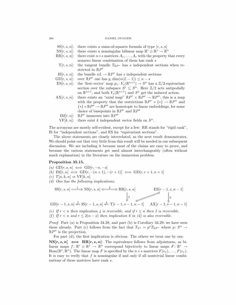
280 DANIEL DUGGER
SS[r, s, n]: there exists a sums-of-squares formula of type [r, s, n]NS[r, s, n]: there exists a nonsingular bilinear map Rr ⊗ Rs → RnRR[r, s, n]: there exist n×smatrices A1, . . . , Ar with the property that every
nonzero linear combination of them has rank sT[r, s, n]: the tangent bundle TRPn has s independent sections when re-
stricted to RP rIS[r, s, n]: the bundle nL→ RP r has s independent sections
GD[r, s, n]: over RP r one has g.dim(n(L− 1)) ≤ n− sES[r, s, n]: the ‘first-vector’ map p1 : Vs(Rn+1)→ Sn has a Z/2-equivariant
section over the subspace Sr ⊆ Sn. Here Z/2 acts antipodallyon Rn+1, and both Vs(Rn+1) and Sn get the induced action.
AX[r, s, n]: there exists an “axial map” RP r × RP s → RPn; this is a mapwith the property that the restrictions RP r × ∗ → RPn and∗×RP s → RPn are homotopic to linear embeddings, for somechoice of basepoints in RP r and RP s
IM[r, n]: RP r immerses into RPnVF[k, n]: there exist k independent vector fields on Sn.
The acronyms are mostly self-evident, except for a few: RR stands for “rigid rank”,IS for “independent sections”, and ES for “equivariant sections”.
The above statements are closely interrelated, as the next result demonstrates.We should point out that very little from this result will be needed in our subsequentdiscussion. We are including it because most of the claims are easy to prove, andbecause the various statements get used almost interchangeably (often withoutmuch explanation) in the literature on the immersion problem.
Proposition 35.15.(a) GD[r, s, n] ⇐⇒ GD[r,−n,−s](b) IM[r, n] ⇐⇒ GD[r,−(n+ 1),−(r + 1)] ⇐⇒ GD[r, r + 1, n+ 1](c) T [n, k, n]⇒ VF[k, n](d) One has the following implications:
SS[r, s, n] 1 +3 NS[r, s, n] ks 2 +3 RR[r, s, n]
3
ES[r − 1, s, n− 1]
6
GD[r − 1, s, n] IS[r − 1, s, n]5ks T[r − 1, s− 1, n− 1]
qy
19kkkkkkkkkkkkk
kkkkkkkkkkkkk4ks AX[r − 1, s− 1, n− 1]
(e) If r < n then implication 4 is reversible, and if r ≤ n then 5 is reversible.(f) If r < n and r ≤ 2(n− s) then implication 6 in (d) is also reversible.
Proof. Part (a) is Proposition 34.28, and part (b) is Corollary 34.29; we have seenthese already. Part (c) follows from the fact that TSn = p∗TRPn where p : Sn →RPn is the projection.
For part (d), the first implication is obvious. The others we treat one by one.NS[r, s, n] ⇐⇒ RR[r, s, n]: The equivalence follows from adjointness, as bi-linear maps f : Rr ⊗ Rs → Rn correspond bijectively to linear maps F : Rr →Hom(Rs,Rn). The linear map F is specified by the n×s matrices F (e1), . . . , F (er).It is easy to verify that f is nonsingular if and only if all nontrivial linear combi-nations of these matrices have rank s.
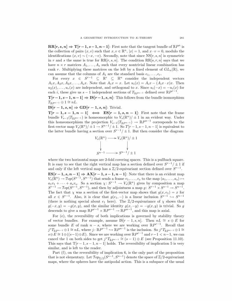
A GEOMETRIC INTRODUCTION TO K-THEORY 281
RR[r, s, n] ⇒ T[r−1, s−1, n−1]: First note that the tangent bundle of RPn isthe collection of pairs (x, v) such that x, v ∈ Rn, |x| = 1, and x · v = 0, modulo theidentifications (x, v) ∼ (−x,−v). Secondly, note that since NS[r, s, n] is symmetricin r and s the same is true for RR[r, s, n]. The condition RR[s, r, n] says that wehave n × r matrices A1, . . . , As such that every nontrivial linear combination hasrank r. Multiplying these matrices on the left by a fixed element of GLn(R), wecan assume that the columns of A1 are the standard basis e1, . . . , er.
For every x ∈ Sr−1 ⊆ Rr ⊆ Rn consider the independent vectorsA1x,A2x,A3x, . . . , Asx. Note that A1x = x. Let ui(x) = Aix − (Aix · x)x. Thenu2(x), . . . , ur(x) are independent, and orthogonal to x. Since ui(−x) = −ui(x) foreach i, these give us s− 1 independent sections of TRPn−1 defined over RP r−1.T[r−1, s−1, n−1] ⇒ IS[r−1, s, n]: This follows from the bundle isomorphismTRPn−1 ⊕ 1 ∼= nL.IS[r − 1, s, n] ⇒ GD[r − 1, s, n]: Trivial.T[r − 1, s − 1, n − 1] ⇐⇒ ES[r − 1, s, n − 1]: First note that the framebundle Vs−1(TRPn−1) is homeomorphic to Vs(Rn)/ ± 1 in an evident way. Underthis homeomorphism the projection Vs−1(TRPn−1) → RPn−1 corresponds to thefirst-vector map Vs(Rn)/± 1→ Sn−1/± 1. So T [r− 1, s− 1, n− 1] is equivalent tothe latter bundle having a section over Sr−1/± 1. But then consider the diagram
Vs(Rn) //
Vs(Rn)/± 1
Sn−1 // Sn−1/± 1
where the two horizontal maps are 2-fold covering spaces. This is a pullback square.It is easy to see that the right vertical map has a section defined over Sr−1/± 1 ifand only if the left vertical map has a Z/2-equivariant section defined over Sr−1.ES[r −1, s, n−1] ⇒ AX[r −1, s−1, n−1]: Note that there is an evident mapVs(Rn)→ Top(Ss−1, Sn−1) that sends a frame v1, . . . , vs to the map (a1, . . . , as) 7→a1v1 + · · · + asvs. So a section χ : Sr−1 → Vs(Rn) gives by composition a mapSr−1 → Top(Ss−1, Sn−1), and then by adjointness a map g : Sr−1 × Ss−1 → Sn−1.The fact that χ was a section of the first-vector map shows that g(x, e1) = x forall x ∈ Sr−1. Also, it is clear that g(e1,−) is a linear inclusion Ss−1 → Sn−1
(there is nothing special about e1 here). The Z/2-equivariance of χ shows thatg(−x, y) = −g(x, y), and the similar identity g(x,−y) = −g(x, y) is trivial. So gdescends to give a map RP r−1 × RP s−1 → RPn−1, and this map is axial.
For (e), the reversibility of both implications is governed by stability theoryof vector bundles. For example, assume IS[r − 1, s, n]. Then nL ∼= s ⊕ E forsome bundle E of rank n − s, where we are working over RP r−1. Recall thatj∗TRPn−1⊕1 ∼= nL, where j : RP r−1 → RPn−1 is the inclusion. So j∗TRPn−1⊕1 ∼=s⊕E ∼= 1⊕((s−1)⊕E). Since we are working over RP r−1 and r−1 < n−1, we cancancel the 1 on both sides to get j∗TRPn−1 ∼= (s − 1) ⊕ E (see Proposition 11.10).This says that T[r− 1, s− 1, n− 1] holds. The reversibility of implication 5 is verysimilar, and is left to the reader.
Part (f), on the reversibility of implication 6, is the only part of the propositionthat is not elementary. Let TopZ/2(Ss−1, Sn−1) denote the space of Z/2-equivariantmaps, where the spheres have the antipodal action. This is a subspace of the usual
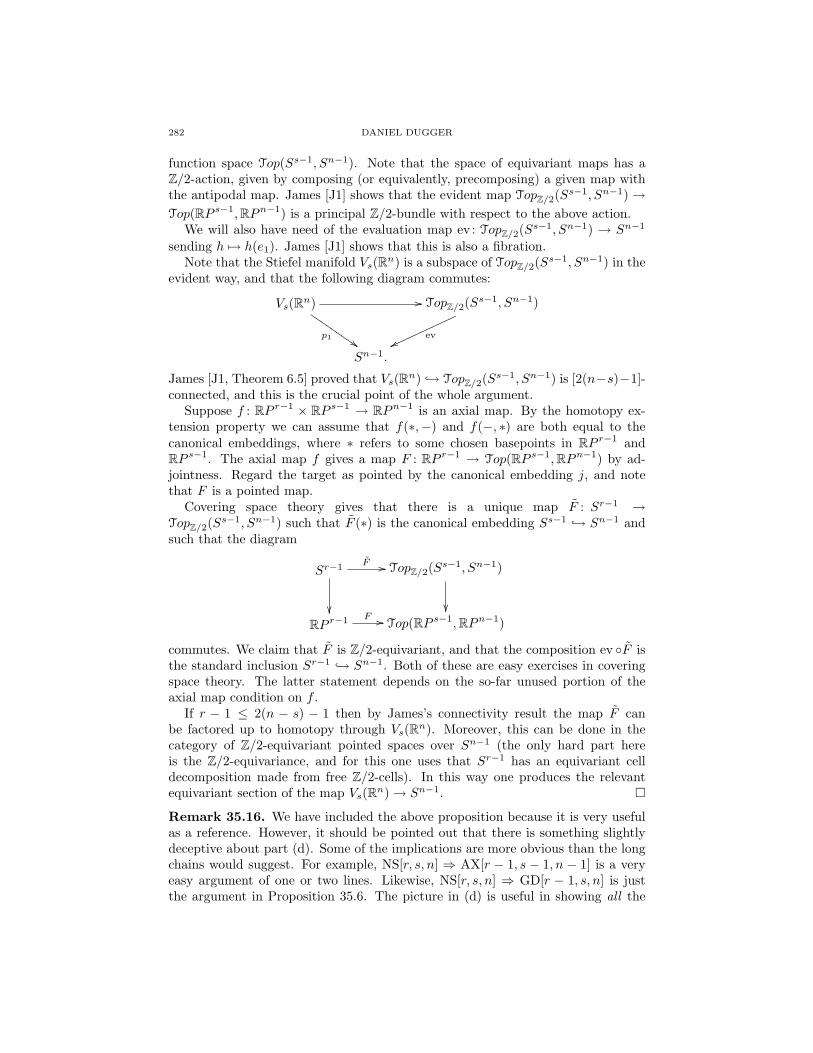
282 DANIEL DUGGER
function space Top(Ss−1, Sn−1). Note that the space of equivariant maps has aZ/2-action, given by composing (or equivalently, precomposing) a given map withthe antipodal map. James [J1] shows that the evident map TopZ/2(Ss−1, Sn−1)→Top(RP s−1,RPn−1) is a principal Z/2-bundle with respect to the above action.
We will also have need of the evaluation map ev : TopZ/2(Ss−1, Sn−1) → Sn−1
sending h 7→ h(e1). James [J1] shows that this is also a fibration.Note that the Stiefel manifold Vs(Rn) is a subspace of TopZ/2(Ss−1, Sn−1) in the
evident way, and that the following diagram commutes:
Vs(Rn) //
p1$$IIIIIIIII
TopZ/2(Ss−1, Sn−1)
evvvnnnnnnnnnnn
Sn−1.
James [J1, Theorem 6.5] proved that Vs(Rn) → TopZ/2(Ss−1, Sn−1) is [2(n−s)−1]-connected, and this is the crucial point of the whole argument.
Suppose f : RP r−1 × RP s−1 → RPn−1 is an axial map. By the homotopy ex-tension property we can assume that f(∗,−) and f(−, ∗) are both equal to thecanonical embeddings, where ∗ refers to some chosen basepoints in RP r−1 andRP s−1. The axial map f gives a map F : RP r−1 → Top(RP s−1,RPn−1) by ad-jointness. Regard the target as pointed by the canonical embedding j, and notethat F is a pointed map.
Covering space theory gives that there is a unique map F : Sr−1 →TopZ/2(Ss−1, Sn−1) such that F (∗) is the canonical embedding Ss−1 → Sn−1 andsuch that the diagram
Sr−1 F //
TopZ/2(Ss−1, Sn−1)
RP r−1 F // Top(RP s−1,RPn−1)
commutes. We claim that F is Z/2-equivariant, and that the composition ev F isthe standard inclusion Sr−1 → Sn−1. Both of these are easy exercises in coveringspace theory. The latter statement depends on the so-far unused portion of theaxial map condition on f .
If r − 1 ≤ 2(n − s) − 1 then by James’s connectivity result the map F canbe factored up to homotopy through Vs(Rn). Moreover, this can be done in thecategory of Z/2-equivariant pointed spaces over Sn−1 (the only hard part hereis the Z/2-equivariance, and for this one uses that Sr−1 has an equivariant celldecomposition made from free Z/2-cells). In this way one produces the relevantequivariant section of the map Vs(Rn)→ Sn−1.
Remark 35.16. We have included the above proposition because it is very usefulas a reference. However, it should be pointed out that there is something slightlydeceptive about part (d). Some of the implications are more obvious than the longchains would suggest. For example, NS[r, s, n] ⇒ AX[r − 1, s − 1, n − 1] is a veryeasy argument of one or two lines. Likewise, NS[r, s, n] ⇒ GD[r − 1, s, n] is justthe argument in Proposition 35.6. The picture in (d) is useful in showing all the
A GEOMETRIC INTRODUCTION TO K-THEORY 283
relations at once, but it makes some of the statements seem more distant than theyreally are.
The reader will have noticed that Proposition 35.15 encodes several things thatwe have seen before. Some are transparently familiar, like parts (a) and (b). A lesstransparent example is
SS[r, n, n] ⇐⇒ SS[n, r, n]⇒ T[n− 1, r − 1, n− 1]⇒ VF[r − 1, n− 1].
This was the content of Corollary 14.9. In constrast, here is a similarly-obtainedimplication that we have not seen yet:
NS[r, r, n]⇒ GD[r − 1, r, n] ⇐⇒ IM[r − 1, n− 1].
From this we learn that immersion results for real projective space can be obtainedby demonstrating the existence of nonsingular bilinear maps. This approach wassuccessfully used by K.Y. Lam in [L1]. We briefly sketch his method simply to givethe basic idea; for details the reader may consult [L1] and similar papers.
Recall that O denotes the octonions. Consider the map f : O2 ×O2 → O3 givenby
f((u1, u2), (x1, x2)
)= (u1x1 − x2u2, x2u1 + u2x1, u2x2 − x2u2).
With a little work one can prove that this is nonsingular. Also, it is a generalfact about the octonions that for any a, b ∈ O the commutator [a, b] = ab − bais imaginary. So the image of f actually lies in the 23-dimensional subspace ofO3 where the real part of the third coordinate vanishes. So f gives a nonsingularbilinear map of type [16, 16, 23]. This shows that RP 15 immerses into R22. Byrestricting f to appropriate subspaces Lam also obtained nonsingular bilinear mapsof types [11, 11, 17], [13, 13, 19], and [10, 10, 16], thereby proving that RP 10 immersesinto R16, RP 12 immerses into R18, and RP 9 immerses into R15.
35.17. Summary. In this section we examined the sums-of-squares problem, andsaw how characteristic classes can be used to obtain lower bounds for the numbersr∗s. Use of Stiefel-Whitney classes in singular cohomology yielded the Hopf-Stiefellower bounds on r ∗ s, whereas the use of the γ-classes in KO-theory gave theYuzvinsky lower bounds. This story is very similar to the one for immersions ofRPn discussed in Section 34, and in fact the sums-of-squares problem is closelyconnected to this immersion problem. We closed the section by exploring therelations between these and a host of similar problems.
284 DANIEL DUGGER
Part 6. Homological intersection theory
36. The theorem of Gillet-Soule
???
Part 7. Appendices
Appendix A. Bernoulli numbers
There are different conventions for naming the Bernoulli numbers, especiallywhen one enters the topology literature. We adopt what seems to be the mostcommon definition, which is the following:
x
ex − 1=
∞∑k=0
Bk ·xk
k!.
Expanding the power series yields
x
ex − 1= 1− x
2+x2
12− x4
720+
x6
30240− x8
1209600+ · · ·
= 1−(1
2
)x+
(16
)· x
2
2−( 1
30
)· x
4
4!+( 1
42
)· x
6
6!−( 1
30
)· x
8
8!· · ·
So we have
k 0 1 2 3 4 5 6 7 8 9
Bk 1 − 12
16 0 − 1
30 0 142 0 − 1
30 0
From the table one guesses that B2n+1 = 0 for n > 0. This is easy to prove: if weset f(x) = x
ex−1 then we can isolate the odd powers of x by examining f(x)−f(−x).But algebra yields ( x
ex − 1
)−( −xe−x − 1
)= −x.
Computing the coefficients of xex−1 is not the most efficient way of computing
Bernoulli numbers, as one can deduce from the large denominators in the aboveformula. A better method is via a certain recursive formula, and this is best re-membered by a “mnemonic”:
(B + 1)n = Bn.(A.1)
Do not take this formula literally! It is shorthand for the following procedure.First expand the left-hand-side via the Binomial Formula, treating B as a formalvariable. Then rewrite the formula by “lowering all indices”, meaning changingevery Bi to a Bi. This gives the desired recursive formula.
For example: (B + 1)2 = B2 yields B2 + 2B + 1 = B2, which in turn givesB2 + 2B1 + 1 = B2. Cancelling the B2’s we obtain 2B1 + 1 = 0, or B1 = − 1
2 .Likewise, (B + 1)3 = B3 yields B3 + 3B2 + 3B1 + 1 = B3, thereby giving
B2 = − 13 (1 + 3B1) = − 1
3 · −12 = 1
6 .
And so on. For the record here are a few more of the Bernoulli numbers, computedin this way:

A GEOMETRIC INTRODUCTION TO K-THEORY 285
k 0 1 2 4 6 8 10 12 14 16 18
Bk 1 − 12
16 − 1
30142 − 1
30566 − 691
273076 − 3617
51043867798
Note that we have not yet justified the recursive formula (A.1). We will do thisafter a short interlude.
A.2. Sums of powers. The Bernoulli numbers first arose in work of JakobBernoulli on computing formulas for the power sums
1t + 2t + 3t + · · ·+ nt.
Most modern students have seen the formulas
1 + 2 + · · ·+ n = n(n+1)2 and 12 + 22 + · · ·+ n2 = n(n+1)(2n+1)
6 .
The Bernoulli formulas generalize these to give
1t + 2t + · · ·+ nt = Pt(n)
where Pt is a degree t+1 polynomial in n with rational coefficients. It is somewhatsurprising that the formulas for the Pt’s can be given using a single set of coefficients,the Bernoulli numbers.
The Bernoulli formulas are most succinctly written using our mnemonic deviceof lowering indices. We write
1t + 2t + · · ·+ nt = 1t+1
[(B + (n+ 1)
)t+1 −Bt+1].(A.3)
Let us work through the first few examples of this. For t = 1 we have
1 + 2 + · · ·+ n = 12
[(B + (n+ 1))2 −B2
]= 1
2
[B2 + 2B1(n+ 1) + (n+ 1)2 −B2
]= 1
2
[(n+ 1)2 − (n+ 1)]
= 12 (n+ 1)n.
For t = 2 we have
12 + 22 + · · ·+ n2 = 13
[(B + (n+ 1))3 −B3
]= 1
3
[3B2(n+ 1) + 3B1(n+ 1)2 + (n+ 1)3
]= 1
3 (n+ 1)[
12 −
32 (n+ 1) + (n+ 1)2
]= 1
3 (n+ 1)[
12n+ n2
]= 1
6 (n+ 1)n(2n+ 1).
We leave it to the reader to derive the t = 3 formula:
13 + 23 + · · ·+ n3 = 14n
2(n+ 1)2.
Proof of the Bernoulli formula (A.3). Start with the identity of power series
1 + ex + e2x + · · ·+ enx =e(n+1)x − 1ex − 1
=( x
ex − 1
)·(e(n+1)x − 1
x
).
The coefficient of xt on the left-hand-side is1t!
(1t + 2t + · · ·+ nt).
286 DANIEL DUGGER
The coefficient of xt on the right-hand-side ist∑
k=0
Bkk!· (n+ 1)t+1−k
(t+ 1− k)!.
Equating coefficients and rearranging yields the Bernoulli formula immediately.
Now let us return to our recursive formula (A.1) for computing the Bernoullinumbers. Note that it is an immediate consequence of (A.3) by taking n = 0 to get0 = (B + 1)t+1 −Bt+1.
A.4. Miscellaneous facts.
Theorem A.5 (Claussen/von Staudt).(a) (−1)nB2n ≡
∑p
1p mod Z, where the sum is taken over all primes p such that
p− 1 divides 2n.(b) When expressed as a fraction in lowest terms, B2n has square-free denominator
consisting of the product of all primes p such that p− 1 divides 2n.
For example, we can now immediately predict that the denominator of B20 willbe 2 · 3 · 5 · 11 = 330. Note that the primes 2 and 3 will always appear in thedenominators of Bernoulli numbers.
The following strange fact is relevant to the appearance of Bernoulli numbers intopology:
Proposition A.6. For any even n and any k ∈ Z, kn(kn−1)Bn
n ∈ Z.
Proof. We follow Milnor and Stasheff here [MS]. Write
f(x) = 1 + ex + e2x + · · ·+ e(k−1)x =ekx − 1ex − 1
.
Note thatf (r)(0) = 1r + 2r + · · ·+ (k − 1)r.
In particular, the derivatives of f evaluated at 0 are all integers.Next consider the logarithmic derivative
f ′(x)f(x)
= D(log(f(x))) =kekx
ekx − 1− ex
ex − 1
= k[ 11− e−kx
]−[ 11− e−x
]=
1x
[ −kxe−kx − 1
− −xe−x − 1
]=
1x
[∑Bi
i! (−kx)i −∑
Bi
i! (−x)i]
=∑i
(−1)i Bi
i! (ki − 1)xi−1
= k−12 + B2
2! (k2 − 1)x+ B44! (k4 − 1)x3 + · · ·
The (2t− 1)st derivative of this expression, evaluated at 0, is B2t
2t (k2t − 1).However, iterated use of the quotient rule shows that the (2t − 1)st derivative
of f ′(x)/f(x), evaluated at 0, can be written as an integral linear combination of
A GEOMETRIC INTRODUCTION TO K-THEORY 287
f(0), f ′(0), f ′′(0), . . . divided by f(0)2t. Since f(0) = k and all the deriviates of fhave integral values at 0, this gives
B2t
2t(k2t − 1) · k2t ∈ Z.
Appendix B. The algebra of symmetric functions
Let S = Z[x1, . . . , xn] be equipped with the evident Σn-action that permutes theindices. It is a well-known theorem that the ring of invariants is a polynomial ringon the elementary symmetric functions:
SΣn ∼= Z[σ1, . . . , σn].
Let sk = xk1 + xk2 + · · ·+ xkn, the kth power sum of the variables xi. Since sk is aΣn-invariant we have
sk = Sk(σ1, . . . , σn)for a unique polynomial Sk in n variables (with integer coefficients). The polynomialSk is called the kth Newton polynomial.
Let us calculate the simplest examples of the Newton polynomials. Clearlys1 = σ1, and so S1(σ1, . . . , σn) = σ1. For s2 we compute that
s2 = x21 + · · ·+ x2
n = (x1 + · · ·+ xn)2 − 2(x1x2 + x1x3 + · · ·+ xn−1xn) = σ21 − 2σ2.
These calculations get more difficult as the exponents get larger.It is useful to adopt the following notation when working with the ring of invari-
ants. If m is a monomial in the xi’s then [m] denotes the sum of all elements in theΣn-orbit of m. For example,
[x1x2] = σ2, [xk1 ] = sk, and [x21x2] =
∑i 6=j
x2ixj .
If H ≤ Σn is the stabilizer of m then we can also write
[m] =∑
g∈Σn/H
gm.
Let us use the above notation to help work out the third Newton polynomial.Elementary algebra easily yields the equation
s3 = [x31] = [x1]3 − 3[x2
1x2]− 6[x1x2x3].
Here one considers the product (x1 + · · ·+ xn)3 and reasons that a term like x21x2
appears three times in the expansion, and terms like x1x2x3 appear six times. Viaa similar process we work out that
[x21x2] = [x1] · [x1x2]− 3[x1x2x3].
Putting everything together, we have found that
s3 = σ31 − 3(σ1σ2 − 3σ3)− 6σ3 = σ3
1 − 3σ1σ2 + 3σ3.
This final expression is the third Newton polynomial S3.
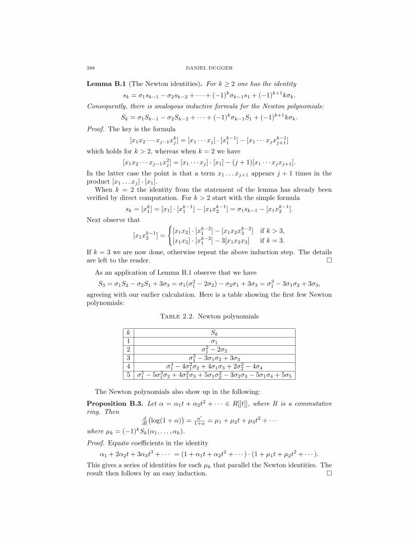
288 DANIEL DUGGER
Lemma B.1 (The Newton identities). For k ≥ 2 one has the identity
sk = σ1sk−1 − σ2sk−2 + · · ·+ (−1)kσk−1s1 + (−1)k+1kσk.
Consequently, there is analogous inductive formula for the Newton polynomials:
Sk = σ1Sk−1 − σ2Sk−2 + · · ·+ (−1)kσk−1S1 + (−1)k+1kσk.
Proof. The key is the formula
[x1x2 · · ·xj−1xkj ] = [x1 · · ·xj ] · [xk−1
1 ]− [x1 · · ·xjxk−1j+1 ]
which holds for k > 2, whereas when k = 2 we have
[x1x2 · · ·xj−1x2j ] = [x1 · · ·xj ] · [x1]− (j + 1)[x1 · · ·xjxj+1].
In the latter case the point is that a term x1 . . . xj+1 appears j + 1 times in theproduct [x1 . . . xj ] · [x1].
When k = 2 the identity from the statement of the lemma has already beenverified by direct computation. For k > 2 start with the simple formula
sk = [xk1 ] = [x1] · [xk−11 ]− [x1x
k−12 ] = σ1sk−1 − [x1x
k−12 ].
Next observe that
[x1xk−12 ] =
[x1x2] · [xk−2
1 ]− [x1x2xk−23 ] if k > 3,
[x1x2] · [xk−21 ]− 3[x1x2x3] if k = 3.
If k = 3 we are now done, otherwise repeat the above induction step. The detailsare left to the reader.
As an application of Lemma B.1 observe that we have
S3 = σ1S2 − σ2S1 + 3σ3 = σ1(σ21 − 2σ2)− σ2σ1 + 3σ3 = σ3
1 − 3σ1σ2 + 3σ3,
agreeing with our earlier calculation. Here is a table showing the first few Newtonpolynomials:
Table 2.2. Newton polynomials
k Sk1 σ1
2 σ21 − 2σ2
3 σ31 − 3σ1σ2 + 3σ3
4 σ41 − 4σ2
1σ2 + 4σ1σ3 + 2σ22 − 4σ4
5 σ51 − 5σ3
1σ2 + 4σ21σ3 + 5σ1σ
22 − 3σ2σ3 − 5σ1σ4 + 5σ5
The Newton polynomials also show up in the following:
Proposition B.3. Let α = α1t + α2t2 + · · · ∈ R[[t]], where R is a commutative
ring. Thenddt
(log(1 + α)
)= α′
1+α = µ1 + µ2t+ µ3t2 + · · ·
where µk = (−1)kSk(α1, . . . , αk).
Proof. Equate coefficients in the identity
α1 + 2α2t+ 3α3t3 + · · · = (1 + α1t+ α2t
2 + · · · ) · (1 + µ1t+ µ2t2 + · · · ).
This gives a series of identities for each µk that parallel the Newton identities. Theresult then follows by an easy induction.
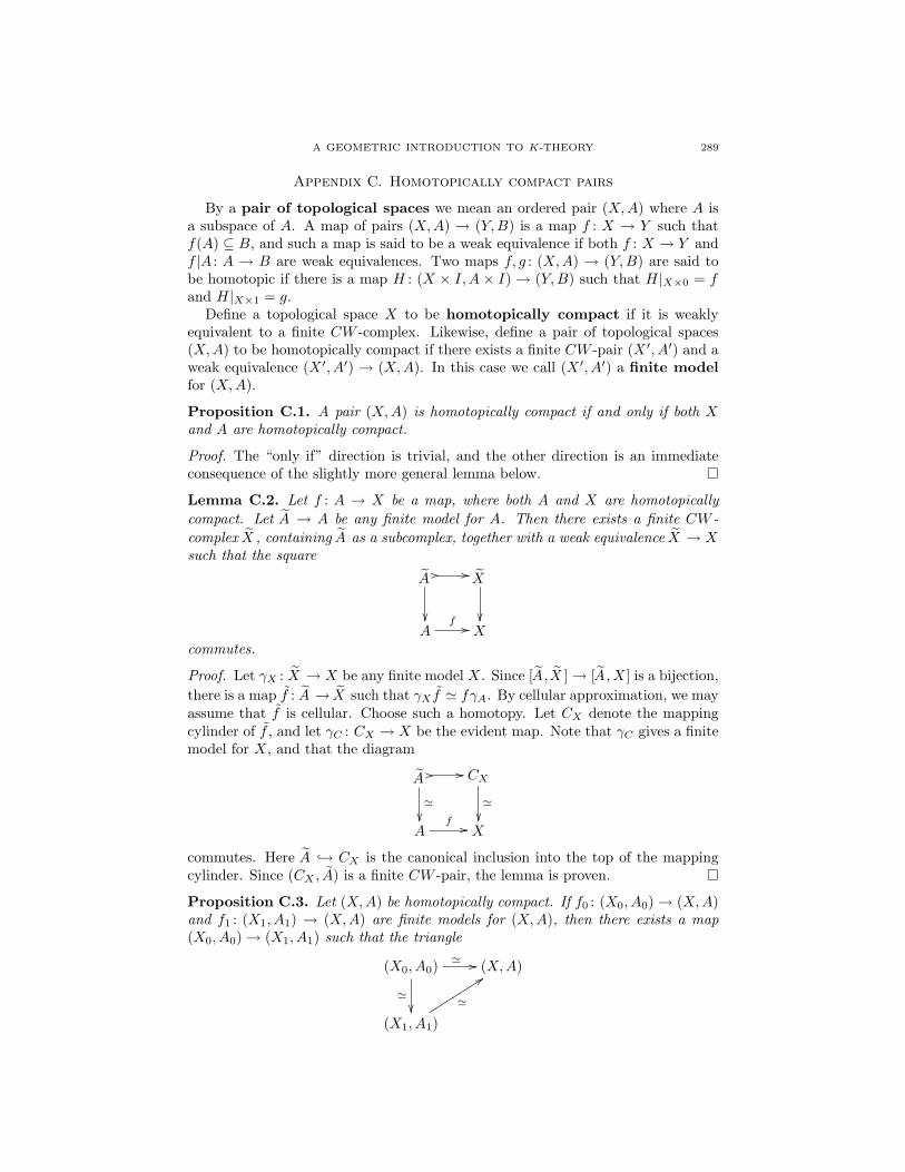
A GEOMETRIC INTRODUCTION TO K-THEORY 289
Appendix C. Homotopically compact pairs
By a pair of topological spaces we mean an ordered pair (X,A) where A isa subspace of A. A map of pairs (X,A) → (Y,B) is a map f : X → Y such thatf(A) ⊆ B, and such a map is said to be a weak equivalence if both f : X → Y andf |A : A → B are weak equivalences. Two maps f, g : (X,A) → (Y,B) are said tobe homotopic if there is a map H : (X × I,A × I) → (Y,B) such that H|X×0 = fand H|X×1 = g.
Define a topological space X to be homotopically compact if it is weaklyequivalent to a finite CW -complex. Likewise, define a pair of topological spaces(X,A) to be homotopically compact if there exists a finite CW -pair (X ′, A′) and aweak equivalence (X ′, A′) → (X,A). In this case we call (X ′, A′) a finite modelfor (X,A).
Proposition C.1. A pair (X,A) is homotopically compact if and only if both Xand A are homotopically compact.
Proof. The “only if” direction is trivial, and the other direction is an immediateconsequence of the slightly more general lemma below.
Lemma C.2. Let f : A → X be a map, where both A and X are homotopicallycompact. Let A → A be any finite model for A. Then there exists a finite CW -complex X , containing A as a subcomplex, together with a weak equivalence X → Xsuch that the square
A // //
X
A
f // Xcommutes.
Proof. Let γX : X → X be any finite model X. Since [A,X ]→ [A,X] is a bijection,there is a map f : A → X such that γX f ' fγA. By cellular approximation, we mayassume that f is cellular. Choose such a homotopy. Let CX denote the mappingcylinder of f , and let γC : CX → X be the evident map. Note that γC gives a finitemodel for X, and that the diagram
A // //
'
CX
'
Af // X
commutes. Here A → CX is the canonical inclusion into the top of the mappingcylinder. Since (CX , A) is a finite CW -pair, the lemma is proven.
Proposition C.3. Let (X,A) be homotopically compact. If f0 : (X0, A0)→ (X,A)and f1 : (X1, A1) → (X,A) are finite models for (X,A), then there exists a map(X0, A0)→ (X1, A1) such that the triangle
(X0, A0)' //
'
(X,A)
(X1, A1)
'
99sssssssss

290 DANIEL DUGGER
commutes up to homotopy. Additionally, there exists a zig-zag of finite models
(Y0, B0) //
'**UUUUUUUUUUUUUUUUUUU (Y1, B1)
'
%%KKKKKKKKK(Y2, B2)
'
oo // · · · (Yr, Br)oo
'uukkkkkkkkkkkkkkk
(X,A)
such that (Y0, B0)→ (X,A) equals (X0, A0)→ (X,A) and (Yr, Br)→ (X,A) equals(X1, A1)→ (X,A). That is, the category of finite models of (X,A) is connected.
Proof. First use that [A0, A1]→ [A0, A] is a bijection to produce a map g : A0 → A1
whose image under the bijection is f0|A. We may assume that g is cellular. Choosea homotopy from f0|A to f1|A g, and using the Homotopy Extension Propertyextend this to a homotopy H : X0 × I → X such that H0 = f0. Let f ′ = H1. Wenow have a commutative diagram
A0//
X1
'
X0f ′ // X
and so by the Relative Homotopy Lifting Property (???) there exists a maph : X0 → X1 such that the upper triangle commutes and the lower triangle com-mutes up to a homotopy relative to A0. And again, we map assume that h is cellular.Putting our two homotopies together, we get the required homotopy-commutativetriangle.
For the final statement of the proposition we can use a four-step zig-zag asfollows:
(X0, A0)i0 //
'f0 ((PPPPPPPPPPP
(X0 × I,A0 × I)
'J
(X0, A0)h //
'f1hvvnnnnnnnnnnn
i1oo (X1, A1)
'f1oo(X,A).
The map labelled J is a homotopy for the triangle in the first part of the proposition.We leave the details for the reader.
For us what is very useful about the class of homotopically compact spaces isthat it includes all algebraic varieties:
Theorem C.4. If X is an algebraic variety over C then X is homotopically com-pact.
Proof. When X is a subvariety of some Cn this is a consequence of [Hir, Theoremon page 170 and Remark 1.10]. For the general case we do an induction on thesize of an affine cover for X. Suppose that U1, . . . , Un is an affine cover, and letA = U2 ∪ · · · ∪ Un. Then we have the pushout diagram
U1 ∩A //
A
U1
// X,
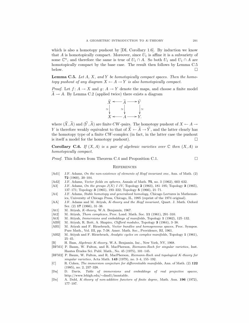
A GEOMETRIC INTRODUCTION TO K-THEORY 291
which is also a homotopy pushout by [DI, Corollary 1.6]. By induction we knowthat A is homotopically compact. Moreover, since U1 is affine it is a subvariety ofsome Cn, and therefore the same is true of U1 ∩ A. So both U1 and U1 ∩ A arehomotopically compact by the base case. The result then follows by Lemma C.5below.
Lemma C.5. Let A, X, and Y be homotopically compact spaces. Then the homo-topy pushout of any diagram X ← A→ Y is also homotopically compact.
Proof. Let f : A → X and g : A → Y denote the maps, and choose a finite modelA → A. By Lemma C.2 (applied twice) there exists a diagram
X
'
A //
'
oo Y
'
X A //oo Y.
where (X ,A) and (Y ,A) are finite CW -pairs. The homotopy pushout of X ← A→Y is therefore weakly equivalent to that of X ← A → Y , and the latter clearly hasthe homotopy type of a finite CW -complex (in fact, in the latter case the pushoutis itself a model for the homotopy pushout).
Corollary C.6. If (X,A) is a pair of algebraic varieties over C then (X,A) ishomotopically compact.
Proof. This follows from Theorem C.4 and Proposition C.1.
References
[Ad1] J.F. Adams, On the non-existence of elements of Hopf invariant one, Ann. of Math. (2)72 (1960), 20–104.
[Ad2] J.F. Adams, Vector fields on spheres, Annals of Math. 75, no. 3 (1962), 603–632.[A3] J.F. Adams, On the groups J(X) I–IV, Topology 2 (1963), 181–195; Topology 3 (1965),
137–171; Topology 3 (1965), 193–222; Topology 5 (1966), 21–71.[A4] J.F. Adams, Stable homotopy and generalised homology, Chicago Lectures in Mathemat-
ics, University of Chicago Press, Chicago, IL, 1995 (reprint of the 1974 original).[AA] J.F. Adams and M. Atiyah, K-theory and the Hopf invariant , Quart. J. Math. Oxford
Ser. (2) 17 (1966), 31–38.[At1] M. Atiyah, K-theory, W.A. Benjamin, 1967.[At2] M. Atiyah, Thom complexes, Proc. Lond. Math. Soc. 11 (1961), 291–310.[At3] M. Atiyah, Immersions and embeddings of manifolds, Topology 1 (1962), 125–132.[ABS] M. Atiyah, R. Bott, A. Shapiro, Clifford modules, Topology 3 (1964), 3–38.[AH1] M. Atiyah and F. Hirzebruch, Vector bundles and homogeneous spaces, Proc. Sympos.
Pure Math., Vol. III, pp. 7-38. Amer. Math. Soc., Providence, RI, 1961.[AH2] M. Atiyah and F. Hirzebruch, Analytic cycles on complex manifolds, Topology 1 (1961),
25–45.[B] H. Bass, Algebraic K-theory, W.A. Benjamin, Inc., New York, NY, 1968.[BFM1] P. Baum, W. Fulton, and R. MacPherson, Riemann-Roch for singular varieties, Inst.
Hautes Etudes Sci. Publ. Math., No. 45 (1975), 101–145.[BFM2] P. Baum, W. Fulton, and R. MacPherson, Riemann-Roch and topological K-theory for
singular varieties, Acta Math. 143 (1979), no. 3–4, 155–192.[C] R. Cohen, The immersion conjecture for differentiable manifolds, Ann. of Math. (2) 122
(1985), no. 2, 237–328.[Da] D. Davis, Table of immersions and embeddings of real projective spaces,
http://www.lehigh.edu/∼dmd1/immtable.[Do] A. Dold, K-theory of non-additive functors of finite degree, Math. Ann. 196 (1972),
177–197.

292 DANIEL DUGGER
[D1] D. Dugger, Multiplicative structures on homotopy spectral sequences I , 2003 preprint,available at arXiv:math/0305173v1.
[D2] D. Dugger, Multiplicative structures on homotopy spectral sequences II , 2003 preprint,available at arXiv:math/0305187v1.
[D3] D. Dugger, Grothendieck groups of complexes with null homotopies, preprint, 2012.[DI] D. Dugger and D. C. Isaksen, Topological hypercovers and A1-realizations, Math. Z. 246
(2004), 667–689.[E] D. Eisenbud, Commutative algebra with a view towards algebraic geometry, Springer-
Verlag, New York, 1995.[FH] H.-B. Foxby and E. B. Halvorson, Grothendieck groups for categories of complexes, J.
K-theory 3 (2009), no. 1, 165–203.[FLS] V. Franjou, J. Lannes, and L. Schwartz, Autour de la cohomologie de MacLane des corps
finis, Invent. Math. 115 (1994), no. 3, 513–538.[F] W. Fulton, Intersection theory, Second edition, Ergebnisse der Mathematik und ihrer
Grenzgebiete, Volume 2, Springer-Verlag, Berlin-Heidelberg, 1998.[GS] H. Gillet and C. Soule, Intersection theory using Adams operations, Invent. Math. 90
(1987), no. 2, 243–277.[G] M. Ginsburg, Some immersions of projective space in Euclidean space, Topology 2 (1963),
69–71.[Gr] D. Grayson, Adams operations on higher K-theory, K-theory 6 (1992), no. 2, 97-111.[GH] P. Griffiths and J. Harris, Principles of algebraic geometry, Wiley Classics Library, John
Wiley & Sons, Inc., New York, 1994.[H] R. Hartshorne, Algebraic geometry, Graduate Texts in Mathematics 52, Springer-Verlag,
New York-Heidelberg, 1977.[Ha] A. Hatcher, Algebraic Topology, Cambridge University Press, 2002.[Ha2] A. Hatcher, Vector bundles and K-theory, preprint. Available on the webpage
http://www.math.cornell.edu/∼hatcher/VBKT/VBpage.html[Hir] H. Hironaka, Triangulations of algebraic sets, Algebraic Geometry (Proc. Sympos. Pure
Math., Vol. 29, Humboldt State Univ., Arcata, Calif., 1974), pp. 165–185. Amer. Math.Soc., Providence, RI, 1975.
[Hi] M. Hirsch, Immersions of manifolds, Trans. Amer. Math. Soc. 93 (1959), no. 2, 242–276.[Ho] H. Hopf, Ein topologischer Beitrag zur reelen Algebra, Comment. Math. Helv. 13 (1940–
41), 219–239.
[Hu] A. Hurwitz, Uber die Komposition der quadratischen Formen von ?????[J1] I.M. James, The space of bundle maps, Topology 2 (1963), 45–59.[L1] K.Y. Lam, Construction of nonsingular bilinear maps, Topology 6 (1967), 423–426.[L2] K.Y. Lam, Topological methods for studying the composition of quadratic forms, Qua-
dratic and Hermition Forms, (Hamilton, Ont., 1983), pp 173–192, Canadian Mathemati-cal Society Conference Proceedings 4, Amer. Math. Soc., 1984.
[LR1] K.Y. Lam and D. Randall,[Mc] J. McCleary, A user’s guide to spectral sequences, Second edition, Cambridge Studies in
Advanced Mathematics 58, Cambridge University Press, Cambridge, 2001.[M] H. Miller, Course Notes: Homotopy theory of the vector field problem, available at
http://www-math.mit.edu/∼hrm/papers/vf1.pdf.[Mi] J. Milnor, Algebraic K-theory, Annals of Mathematics Studies 72, Princeton University
Press, Princeton, NJ, 1971.[MS] J. Milnor and J. Stasheff, Characteristic classes, Princeton University Press, 1974.[MT] R.E. Mosher and M.C. Tangora, Cohomology operations and applications in homotopy
theory, Dover Books on Mathematics, 2008.[Q] D. Quillen, Higher algebraic K-theory: I , Lecture Notes in Mathematics 341, Springer-
Verlag, 85–147.[R] P. Roberts, ????[Sa1] B.J. Sanderson, Immersions and embeddings of projective spaces, Proc. London. Math.
Soc. (3) 14 (1964), 137–153.[Sa2] B.J. Sanderson, A non-immersion theorem for real projective spaces, Topology 2 (1963),
209–211.[S] J.P. Serre, Algebre locale. Multiplicites, Lecture Notes in Math. 11, Springer-Verlag,
Berlin-New York, 1965.
A GEOMETRIC INTRODUCTION TO K-THEORY 293
[St] E. Stiefel, Uber Richtungsfelder in den projektiven Raumen und einen Satz aus der reelenAlgebra, Comment. Math. Helv. 13 (1940/41), 201–218.
[Sw] R. Swan, Vector bundles and projective modules, Trans. Amer. Math. Soc. 105, no. 2(1962), 264–277.
[Swz] R. M. Switzer, Algebraic topology—homotopy and homology, Classics in Mathematics,Springer-Verlag, Berlin, 2002 (reprint of the 1975 original).
[T] B. Totaro, Torsion algebraic cycles and complex cobordism, J. Amer. Math. Soc. 10(1997), no. 2, 467–493.
[Wh1] H. Whitney, The self-intersections of a smooth n-manifold in 2n-space, Ann. of Math.(2) 45 (1944), 220–246.
[Wh2] H. Whitney, The singularities of a smooth n-manifold in (2n− 1)-space, Ann. of Math.(2) 45 (1944), 247–293.
[Y] S. Yuzvinsky, Orthogonal pairings of Euclidean spaces, Michigan Math. J. 28 (1981),131–145.
Department of Mathematics, University of Oregon, Eugene, OR 97403