OpenSeesOpenSees--SNOPT: A Framework for SNOPT: A Framework for Finite Element Based OptimizationFinite Element Based Optimization

Joel Conte, Philip Gill, Yong LiJoel Conte, Philip Gill, Yong LiUniversity of California, San Diego, CAUniversity of California, San Diego, CA

Quan GuQuan GuXiamenUniversity, Xiamen, P.R. ChinaXiamenUniversity, Xiamen, P.R. China

Michele BarbatoMichele BarbatoLouisiana State University, Baton Rouge, LALouisiana State University, Baton Rouge, LA

Frank McKennaFrank McKennaUniversity of California, Berkeley, CAUniversity of California, Berkeley, CA

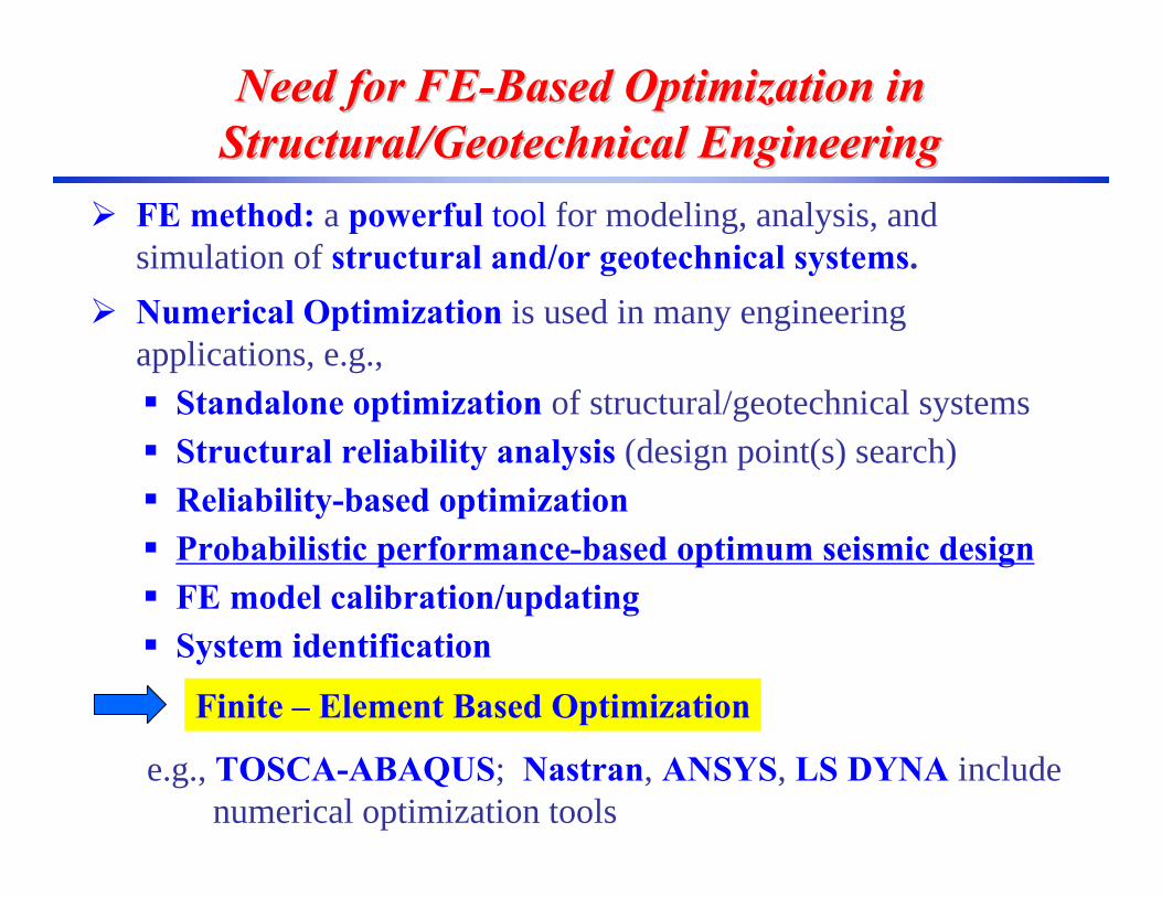
Need for FENeed for FE--Based Optimization in Based Optimization in Structural/Geotechnical Engineering Structural/Geotechnical Engineering

FE method: a powerful tool for modeling, analysis, and simulation of structural and/or geotechnical systems.Numerical Optimization is used in many engineering applications, e.g.,

Standalone optimization of structural/geotechnical systemsStructural reliability analysis (design point(s) search)Reliability-based optimizationProbabilistic performance-based optimum seismic designFE model calibration/updatingSystem identification

Finite – Element Based Optimization

e.g., TOSCA-ABAQUS; Nastran, ANSYS, LS DYNA include numerical optimization tools

Optimization Problems in Optimization Problems in Structural/Geotechnical EngineeringStructural/Geotechnical Engineering

Are complex in nature and stem from a broad range of applications.Involve FE response of structural, geotechnical, or SFSI systems to various static and/or dynamic loads.Require optimization of different system properties (e.g., modal frequencies, mode shapes, damping properties) and/or system response behavior (e.g., force-deformation relationships, various features of displacement/velocity/acceleration response histories).Objective Functions, e.g., weight, initial cost, life cycle cost, demand hazard curve, reliability index, loss hazard curve. Constraints, e.g., geometry, max. displ./accel./stress response, max. plastic deformation, reliability index.

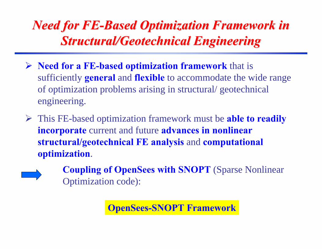
Need for FENeed for FE--Based Optimization Framework in Based Optimization Framework in Structural/Geotechnical EngineeringStructural/Geotechnical Engineering

Need for a FE-based optimization framework that is sufficiently general and flexible to accommodate the wide range of optimization problems arising in structural/ geotechnical engineering.

This FE-based optimization framework must be able to readily incorporate current and future advances in nonlinear structural/geotechnical FE analysis and computational optimization.

Coupling of OpenSees with SNOPT (Sparse Nonlinear Optimization code):

OpenSees-SNOPT Framework

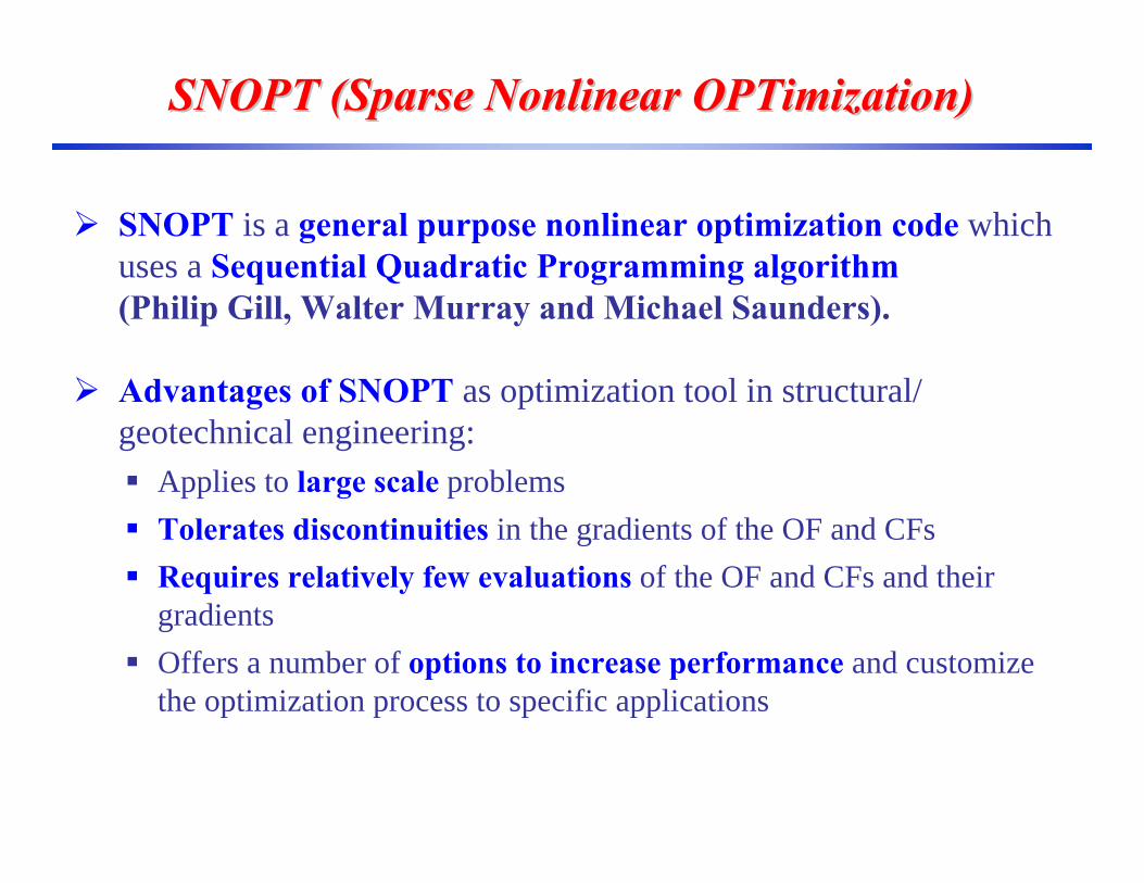
SNOPT (Sparse Nonlinear OPTimization)SNOPT (Sparse Nonlinear OPTimization)

SNOPT is a general purpose nonlinear optimization code which uses a Sequential Quadratic Programming algorithm(Philip Gill, Walter Murray and Michael Saunders).

Advantages of SNOPT as optimization tool in structural/ geotechnical engineering:

Applies to large scale problemsTolerates discontinuities in the gradients of the OF and CFsRequires relatively few evaluations of the OF and CFs and their gradientsOffers a number of options to increase performance and customize the optimization process to specific applications

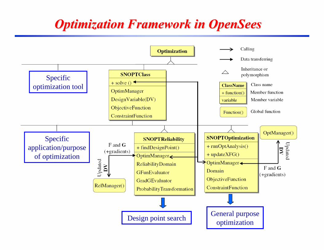
Optimization Framework in OpenSeesOptimization Framework in OpenSees

Specific optimization tool

Specific application/purpose

of optimization

Design point search General purpose optimization

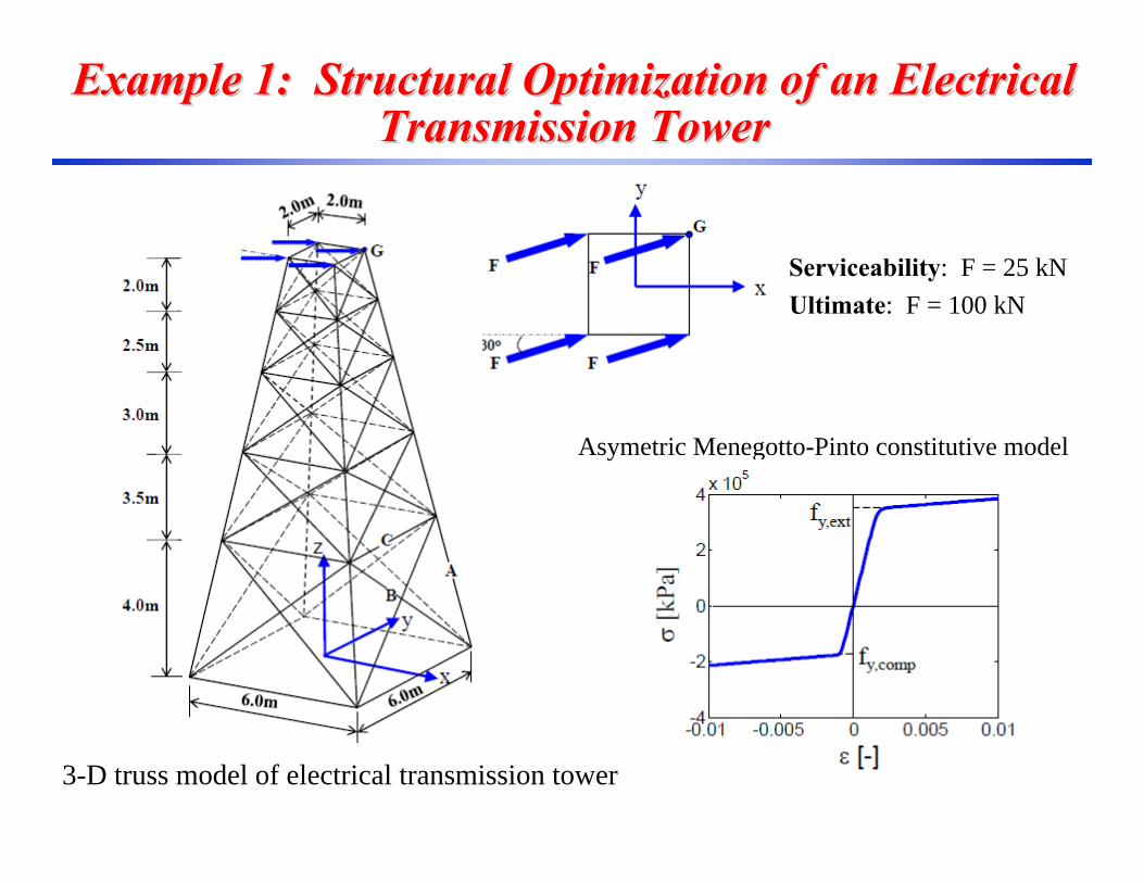
Example 1: Structural Optimization of an Electrical Example 1: Structural Optimization of an Electrical Transmission TowerTransmission Tower

3-D truss model of electrical transmission tower

Asymetric Menegotto-Pinto constitutive model

Serviceability: F = 25 kNUltimate: F = 100 kN

(1) when F = 25 kN, umax < 1.50 cm (at the top of the tower) (2) when F = 100 kN, umax < 15.0 cm (at the top of the tower)

Minimize the total cost (or volume) of the tower such that

Design variables(1) Cross-section Area A: in range [8.0e-4, 1.6e-2] m2 , initial 8e-3 m2

(2) Cross-section Area B: in range [3.0e-4, 6.0e-3] m2 , initial 3e-3 m2

(3) Cross-section Area C: in range [2.0e-4, 4.0e-3] m2 , initial 2e-3 m2

(1) A = 3.17e-3 m2, B = 3.51e-4 m2, C = 2.00e-4 m2

(2) Total volume = 0.274 m3 (compared with initial volume of 1.20m3 ).

Optimal design

Optimization Problem and Solution Optimization Problem and Solution

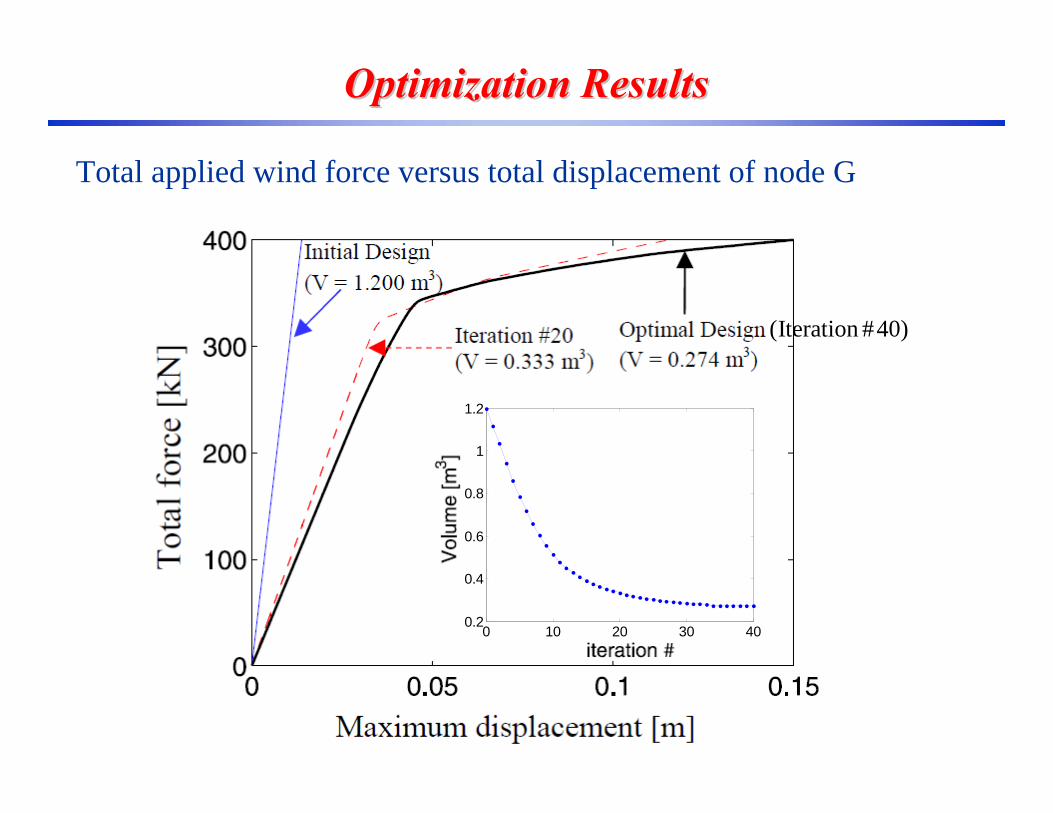
Optimization Results Optimization Results

Total applied wind force versus total displacement of node G

(Iteration #40)

0 10 20 30 400.2

0.4

0.6

0.8

1

1.2

2D soil column modeled by three layers of pressure-independent multi-yield surface J2 soil plasticity models

Example 2: Nonlinear FE Model Updating of Soil Example 2: Nonlinear FE Model Updating of Soil ColumnColumn

Kinematics: shear column

Reference material properties

Input motion: the downhole acceleration record (#12 N-S direction at 17 m depth) obtained during the Lotung China earthquake of 1986

G1(MPa) 28.8 τmax,1 (kPa) 31.0

G2(MPa) 39.2 τmax,2 (kPa) 33.0

G3(MPa) 57.8 τmax,3 (kPa) 34.0

Base acceleration time history

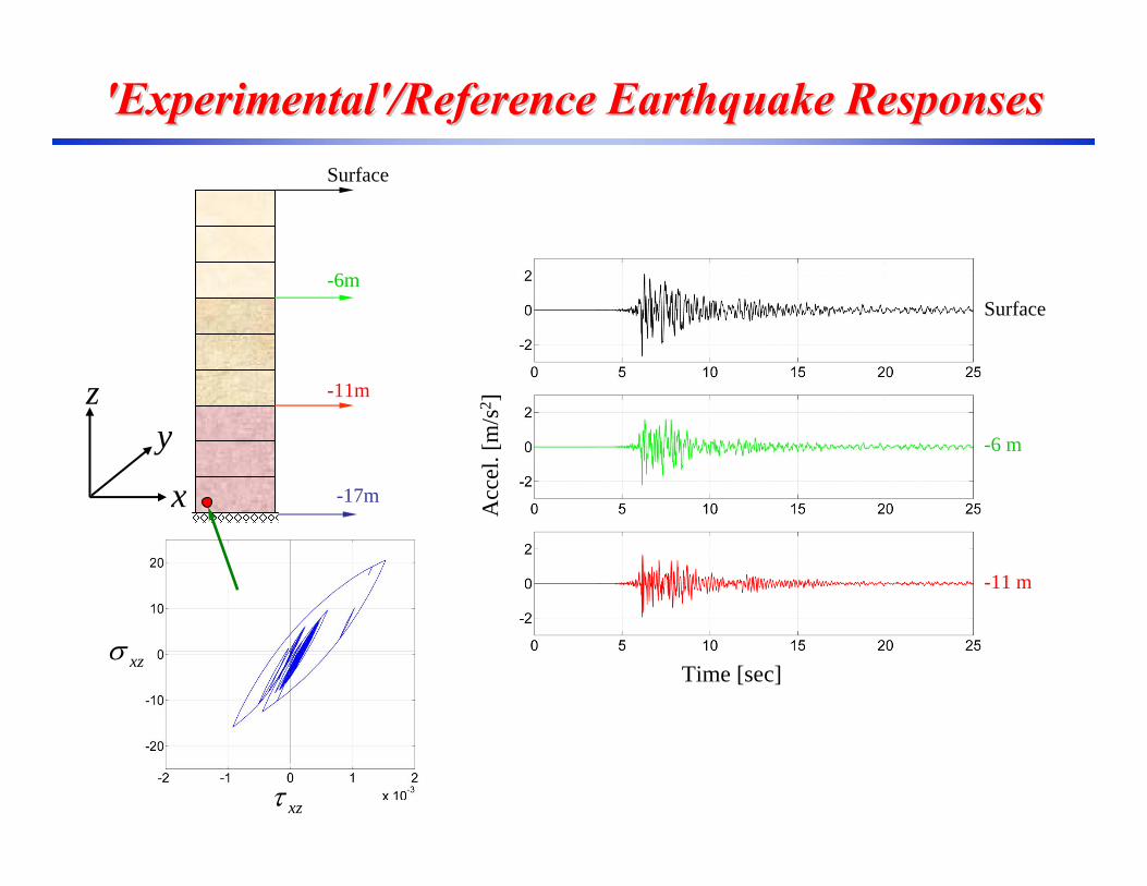
'Experimental'/Reference Earthquake Responses'Experimental'/Reference Earthquake Responses

xzσ

xzτ

-6m

-11m

-17m

Surface

x

zy

Surface

-6 m

-11 m

Time [sec]

Acc

el. [

m/s

2 ]

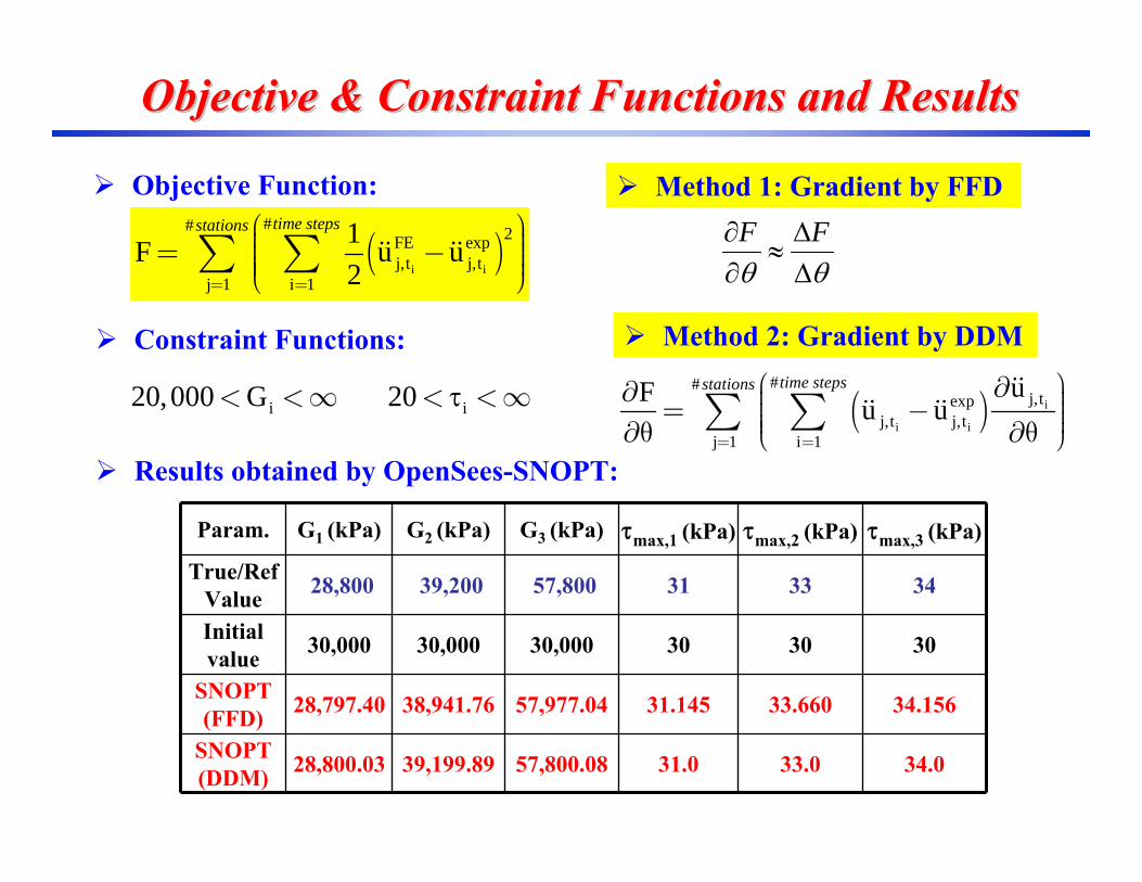
Objective & Constraint Functions and ResultsObjective & Constraint Functions and Results

Objective Function:

Constraint Functions:

i20,000 G< <∞

( )i i

## 2FE expj,t j,t

j 1 i 1

1F u u2

time stepsstations

= =

⎛ ⎞⎟⎜ ⎟= −⎜ ⎟⎜ ⎟⎜⎝ ⎠∑ ∑

Method 1: Gradient by FFD

θθ ΔΔ

≈∂∂ FF

Method 2: Gradient by DDM

( ) i

i i

##j,texp

j,t j,tj 1 i 1

uF u utime stepsstations

= =

⎛ ⎞∂∂ ⎟⎜ ⎟= −⎜ ⎟⎜ ⎟⎜∂θ ∂θ⎝ ⎠∑ ∑

Param. G1 (kPa) G2 (kPa) G3 (kPa) τmax,1 (kPa) τmax,2 (kPa) τmax,3 (kPa)

True/Ref Value 28,800 39,200 57,800 31 33 34

Initial value 30,000 30,000 30,000 30 30 30

SNOPT(FFD) 28,797.40 38,941.76 57,977.04 31.145 33.660 34.156

SNOPT(DDM) 28,800.03 39,199.89 57,800.08 31.0 33.0 34.0

Results obtained by OpenSees-SNOPT:

i20< <∞τ

Time [sec]

]/[ 2smu g

(a)

(b)

Comparison between ‘experimental’ (reference) and FE predicted ground surface accelerations: (a) before FE model updating, (b) after FE model updating

Comparison of Ground Acceleration after FE Comparison of Ground Acceleration after FE model Updating (DDM)model Updating (DDM)

]/[ 2smu g

F = 2.8E-4F = 398.10Initial value of

objective functionFinal value of objective function

Convergence Process (DDM versus FFD)Convergence Process (DDM versus FFD)

( )i i

## 2expj,t j,t

j 1 i 1

1F u u2

time stepsstations

= =

⎛ ⎞⎟⎜ ⎟= −⎜ ⎟⎜ ⎟⎜⎝ ⎠∑ ∑

Note: FE model updating converges MUCH FASTER using DDM versus FFD.

Iteration #

F

Example 3: FE Reliability Analysis of R/C Frame Example 3: FE Reliability Analysis of R/C Frame StructureStructure

30 25

y2025

A

7.0 7.0CC

CCB

B

B

B

A

A

P

P/2

(unit: m)

3.6

7.2

z20 25

y2025

B

z20 20

25

C

z

y20

(unit: cm)30 25

y2025

A

7.0 7.0CC

CCB

B

B

B

A

A

P

P/2

(unit: m)

3.6

7.2

z20 25

y2025

B

z20 20

25

C

z

y20

(unit: cm)

Two-story two-bay R/C frame model

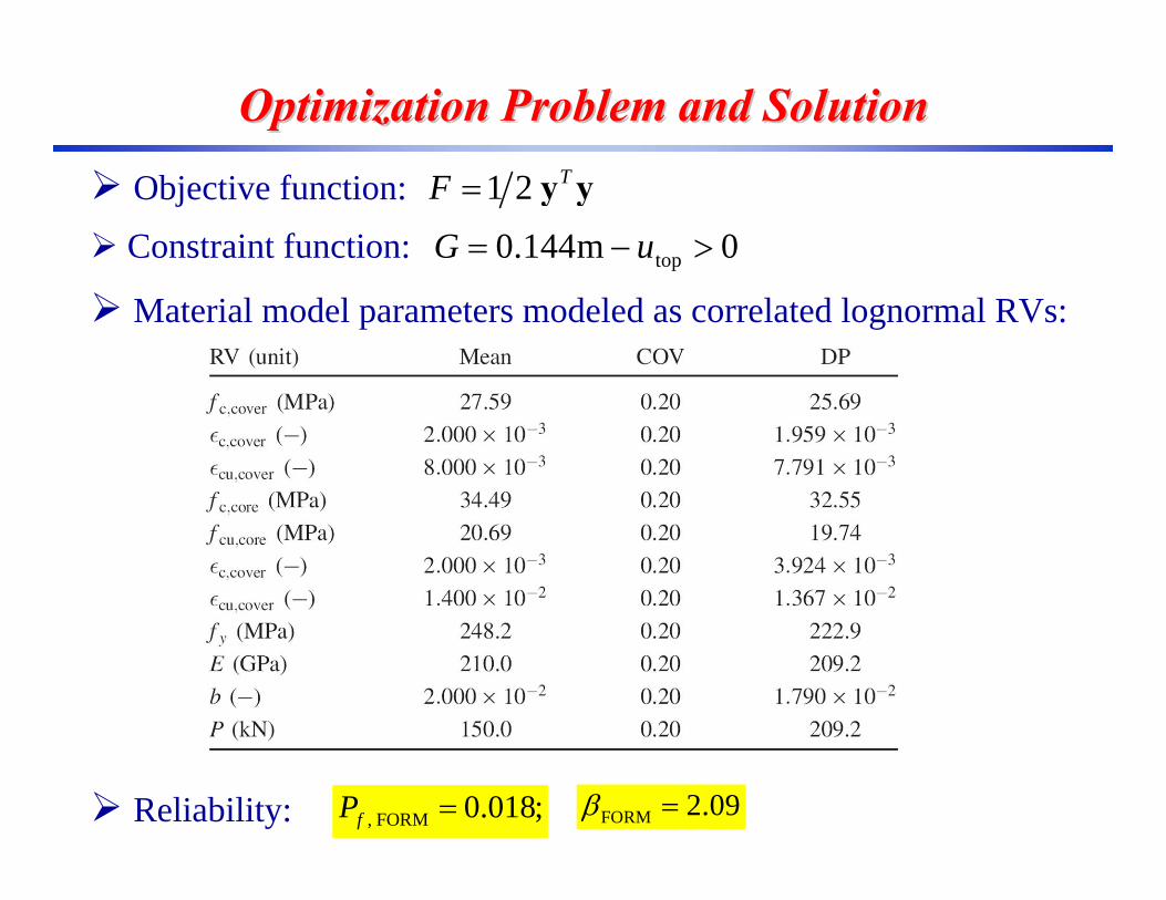
Material model parameters modeled as correlated lognormal RVs:

Objective function:

Constraint function:

1 2 TF y y=

top0.144m 0G u= − >

, FORM 0.018;fP = FORM 2.09β =Reliability:

Optimization Problem and Solution Optimization Problem and Solution

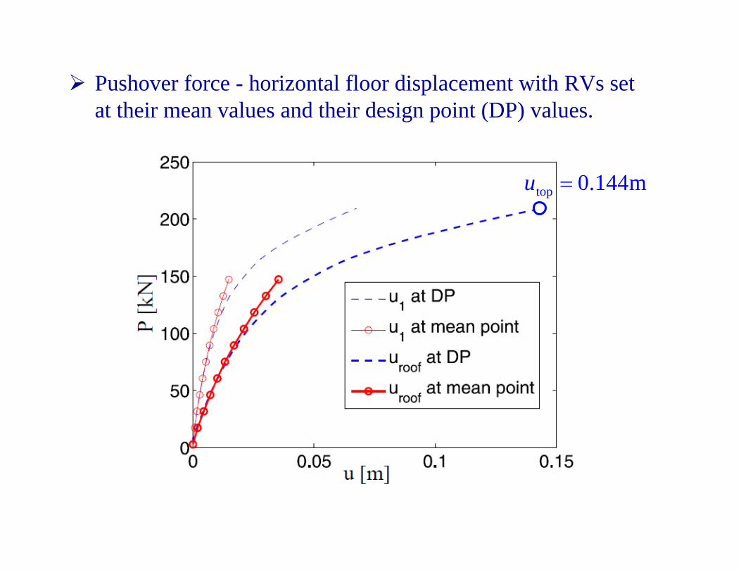
Pushover force - horizontal floor displacement with RVs set at their mean values and their design point (DP) values.

top 0.144mu =

Example 4: Probabilistic PerformanceExample 4: Probabilistic Performance--based Optimum based Optimum Seismic DesignSeismic Design

18

6,150 tons0.100.02

mbξ

===

SDOF Model (Menegotto-Pinto)

SDOF Model (Menegotto-Pinto)

0k

F

U

yF

0.075 myU =

1

1 0b k⋅

*0

*

137,200 kN/m

10,290 kNy

k

F

=

=

PBEE AnalysisPBEE

Analysis

A priori selected optimum design parameters

A priori selected optimum design parameters

Starting PointStarting Point0 100,000 kN/m

14,000 kNy

kF=

=

( )0, TL yk Fν

T

ObjLν

( )

∑ T T

0 y

Obj 2L 0 y L

i

Objective function : f k , F

= | ν (k , F ) - ν |

Expected OptimizerExpected Optimizer OpenSees-SNOPT

OpenSees-SNOPT

• Optimization Problem:

• Starting Point:

• Objective Function Plot:

Problem Formulation and Objective Function Problem Formulation and Objective Function

{ }( )

00

,

0

,

: 80,000 187, 200 (kN/m) 6,290 15,290 ( )

yy

k F

y

Minimize f k F

subject tok

F kN≤ ≤≤ ≤

(0) (0)0 100,000 kN/m, 14,000kN yk F= =

•Obj

ectiv

e Fu

nctio

n

Zoom •Obj

ectiv

e Fu

nctio

n

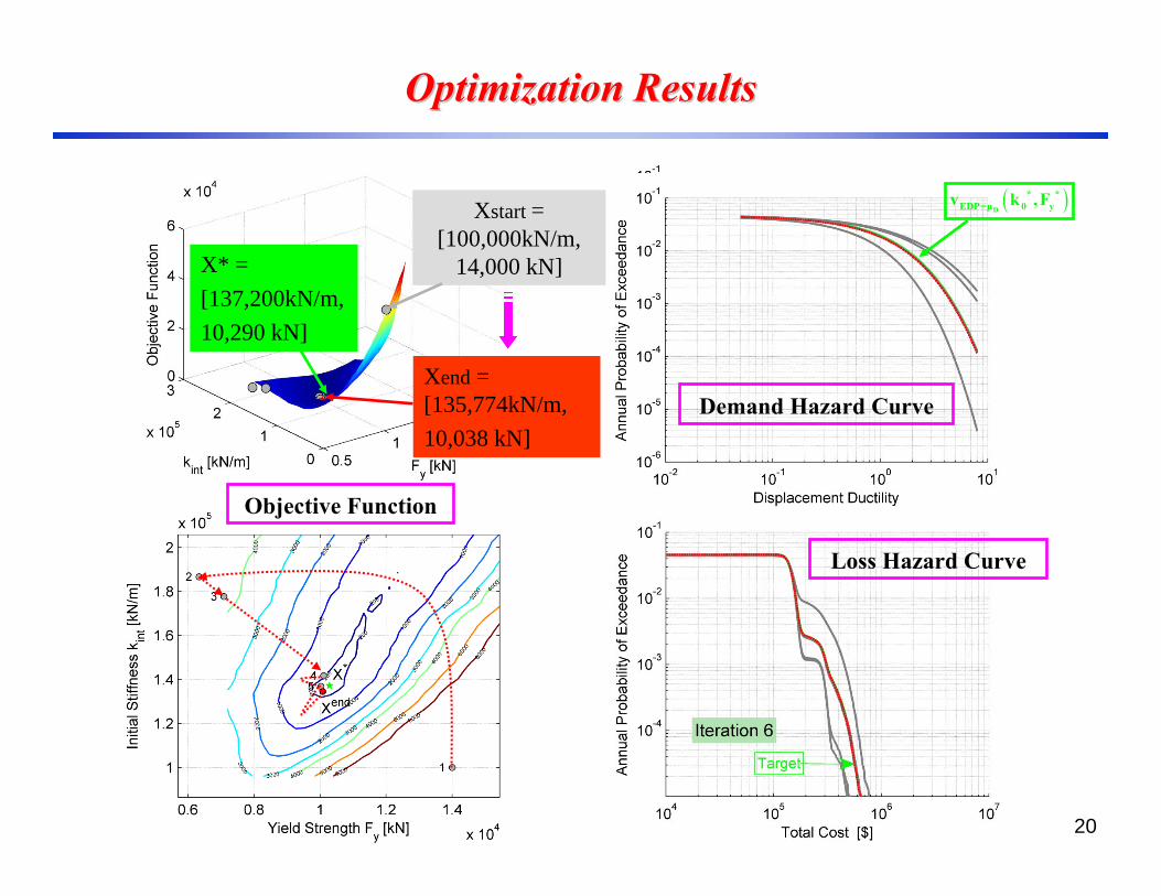
Optimization ResultsOptimization Results

20

Loss Hazard Curve

Demand Hazard Curve

Objective Function

( )D

* *EDP=μ 0 yv k ,F

X* = [137,200kN/m,10,290 kN]

Xstart = [100,000kN/m,

14,000 kN]

Xend = [135,774kN/m,10,038 kN]

Current research based on applicationof OpenSees-SNOPT

Investigation of Seismic Isolation for CHSR Prototype BridgeInvestigation of Seismic Isolation for CHSR Prototype Bridge

California High-Speed Train Project (CHST)

Arial/Bridge Structure Supporting System

Seismic Isolation System (SIS)

PEER Performance-based Earthquake Engineering (PBEE) Methodology

Probabilistic Performance-based Optimization of SIS

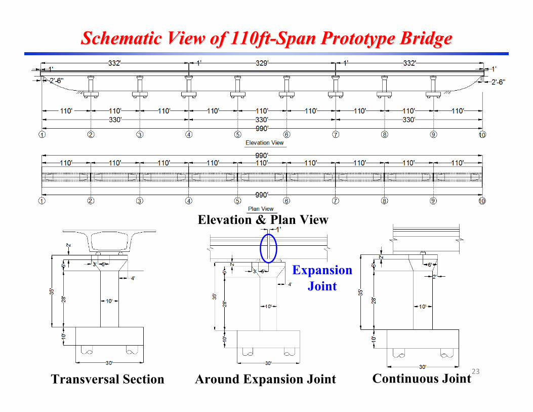
Schematic View of 110ftSchematic View of 110ft--Span Prototype BridgeSpan Prototype Bridge

23

Elevation & Plan View

Around Expansion Joint Continuous Joint

ExpansionJoint

Transversal Section

Gu, Q., Barbato, M., Conte, J. P., Gill, P. E., and McKenna, F., “OpenSees-SNOPT Framework for Finite-Element-Based Optimization of Structural and Geotechnical Systems,” Journal of Structural Engineering, ASCE, 138(6), 822-834, 2012.

Thank you !