consumption and the great recession -...
TRANSCRIPT
NBER WORKING PAPER SERIES
CONSUMPTION AND THE GREAT RECESSION
Mariacristina De NardiEric French
David Benson
Working Paper 17688http://www.nber.org/papers/w17688
NATIONAL BUREAU OF ECONOMIC RESEARCH1050 Massachusetts Avenue
Cambridge, MA 02138December 2011
We thank Richard Porter and an anonymous referee for helpful comments and Helen Koshy for editorialadvice. The views expressed in this paper are those of the authors and not necessarily those of theFederal Reserve Bank of Chicago, the Federal Reserve System, or the National Bureau of EconomicResearch.
NBER working papers are circulated for discussion and comment purposes. They have not been peer-reviewed or been subject to the review by the NBER Board of Directors that accompanies officialNBER publications.
© 2011 by Mariacristina De Nardi, Eric French, and David Benson. All rights reserved. Short sectionsof text, not to exceed two paragraphs, may be quoted without explicit permission provided that fullcredit, including © notice, is given to the source.

Consumption and the Great RecessionMariacristina De Nardi, Eric French, and David BensonNBER Working Paper No. 17688December 2011, Revised February 2012JEL No. E10,E21,E31,H31
ABSTRACT
We document some key facts about aggregate consumption and its subcomponents over time. Wethen document the behavior of some important determinants of consumption, such as consumers’ expectationsabout their future income, and changes in the consumers’ wealth positions. Finally, we use a simplepermanent income model to show that the observed drop in consumption during the Great Recessioncan be explained by the observed drops in wealth and income expectations.
Mariacristina De NardiFederal Reserve Bank of Chicago230 South LaSalle St.Chicago, IL 60604and [email protected]
Eric FrenchResearch DepartmentFederal Reserve Bank of Chicago230 South LaSalle StreetChicago, IL [email protected]
David Benson230 S. La Salle St.Chicago, IL [email protected]
2
Introduction
The Great Recession of 2008/2009 was characterized by the most severe year over year
decline in consumption since 1945. The consumption slump was both deep and long lived. It
took almost 12 quarters for total real Personal Consumption Expenditures (PCE) to go back to
its level at the previous peak (2007:Q4).
This article documents key facts about aggregate consumption and its subcomponents
over time and looks at the behavior of important determinants of consumption, such as
consumers’ expectations about their future income, and changes in the consumers’ wealth
positions due to changes in house prices and stock valuation. Then, the article uses a simple
permanent income model to determine whether the observed drop in consumption can be
explained by the observed drops in wealth and income expectations.
The data analysis starts by using macroeconomic data to study the behavior of
consumption and its subcomponents. The analysis then turns to microeconomic data from the
University of Michigan Survey of Consumers to study nominal expected income growth and
inflationary expectations.
Our main findings from the Macro data are the following. First, the Great Recession
marked the most severe and persistent decline in aggregate consumption since WWII. All
subcomponents of consumption declined during this period. However, the large drop in
services consumption stands out most compared to previous recessions. Second, while the
decline was historic, the time path of consumption and its subcomponents leading up the
recession was not substantially different from past recessionary periods. Third, the recovery
path of consumption following the Great Recession has been uncharacteristically weak. It took
nearly three years for total consumption to return to its level just prior to the recession. In
contrast, the second worst rebound observed in the data followed the 1974 recession and
lasted just over one year. We find that this persistence is reflected most in the subcomponents
of non-durables and especially services consumption.
Our main findings from the analysis of the Micro data are as follows. First, expected
nominal income growth declined significantly during the Great Recession. It is the worst drop
ever observed in these data, and it has not yet fully recovered to pre-recession levels. Second,

3
the decline exists for all age groups, education levels, and income quintiles. Relative to
previous recessions, however, those with higher levels of income and education are more
pessimistic than their poorer and less educated counterparts. Third, expectations for real
income growth have also declined, and the decline in expected real income growth is more
severe when personal inflation expectations are used instead of actual CPI inflation. Fourth,
expected income growth is a strong predictor of actual future income growth. Since expected
income growth is a very important determinant of consumption decisions, the observed drop in
expected income has the potential to explain at least part of the observed decline in
consumption.
In the context of a simple permanent income model, we find that the negative wealth
effect (coming from decreased stock market valuation and housing prices) and decreased
consumers’ income expectations were big factors in determining the observed consumption
drop. In fact, we find that in this model the observed drops in wealth and income expectations
can explain the observed drop in consumption in its entirety, depending on what is assumed
about future income growth going forward, beyond the time horizon covered by the Michigan
Survey of Consumers data set.
Macro data: total real PCE
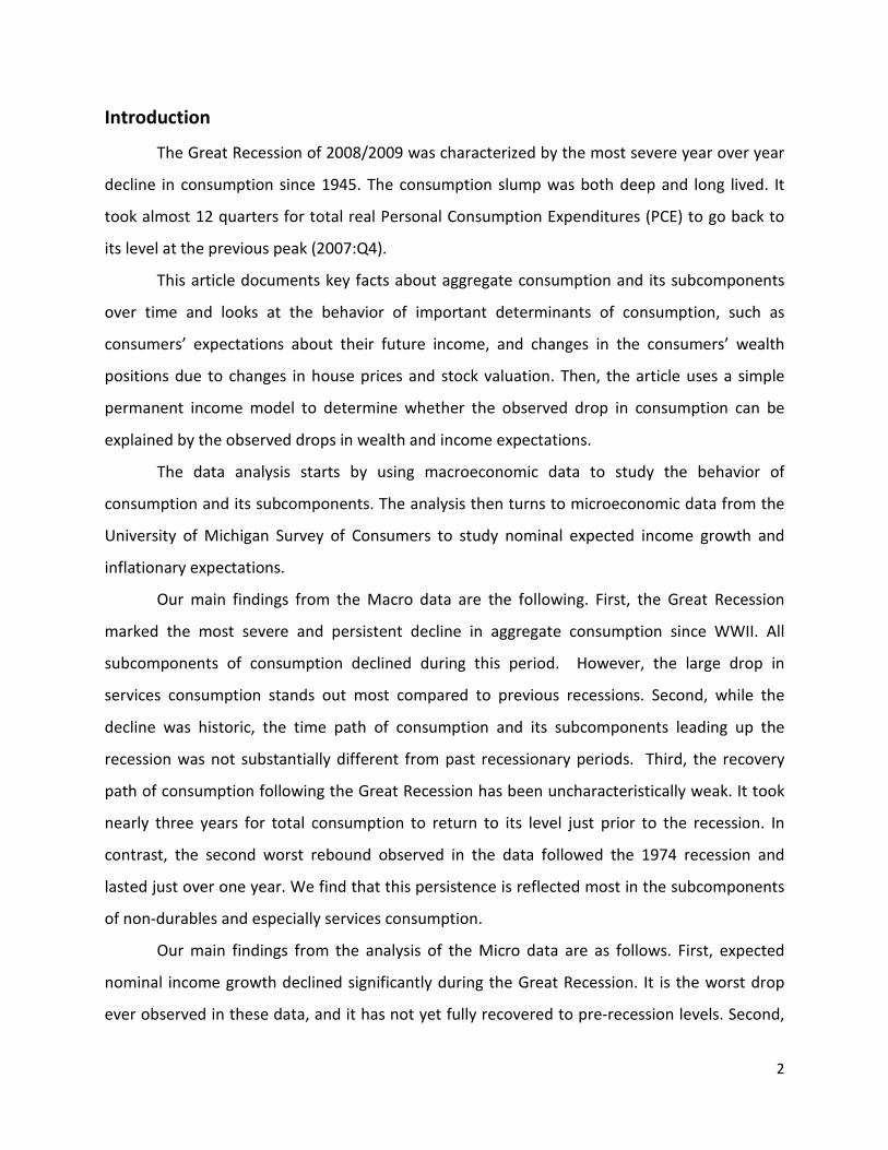
Figure 1 displays the level of real PCE from 1962 to 2011:Q3. Even over this long
horizon, the chart shows a flattening out of the consumption growth rate in 2008/2009. The
fact that this pattern is clearly visible even over a period of almost 50 years highlights the
severity and persistence of the Great Recession and the very slow recovery that is following it.
Fig. 1 Level of real PCE in 2005 dollars, in billions.
4
Figure 2 shows that consumption growth outpaced GDP growth through past
recessionary periods. The nominal PCE-GDP ratio increases in each recession since 1962. In
contrast, during the Great Recession, it increased more modestly. Even after the recession, this
ratio has either fallen or stagnated. Thus, as a share of GDP, consumption has been hit harder
than in previous recessions.
Figure 2. Nominal PCE to nominal GDP ratio with NBER recession shading since 1962.
0 1000 2000 3000 4000 5000 6000 7000 8000 9000
10000
1962
:01
1964
:01
1966
:01
1968
:01
1970
:01
1972
:01
1974
:01
1976
:01
1978
:01
1980
:01
1982
:01
1984
:01
1986
:01
1988
:01
1990
:01
1992
:01
1994
:01
1996
:01
1998
:01
2000
:01
2002
:01
2004
:01
2006
:01
2008
:01
2010
:01
Billi
ons o
f $20
05
Figure 1: Historical level of real PCE, in billions ($2005)
Real PCE Levels ($2005)
0.54
0.56
0.58
0.6
0.62
0.64
0.66
0.68
0.7
0.72
1962
:Q1
1963
:Q4
1965
:Q3
1967
:Q2
1969
:Q1
1970
:Q4
1972
:Q3
1974
:Q2
1976
:Q1
1977
:Q4
1979
:Q3
1981
:Q2
1983
:Q1
1984
:Q4
1986
:Q3
1988
:Q2
1990
:Q1
1991
:Q4
1993
:Q3
1995
:Q2
1997
:Q1
1998
:Q4
2000
:Q3
2002
:Q2
2004
:Q1
2005
:Q4
2007
:Q3
2009
:Q2
2011
:Q1
PCE
- GDP
ratio
Figure 2: Nominal PCE-GDP ratio

5
Petev, Pistaferri, and Ecksten (2010) document that, while real per-capita consumption
declines monotonically until the middle of 2009, real per-capita disposable income is relatively
stable and that its decline was significantly smaller. This stability in per-capita income is
explained entirely by a strong increase in government transfers to households, as wage and
financial income fell. The increase in government transfers was partly due to higher take-up
rates for unemployment insurance and food stamps, and partly due to the increased generosity
of means-tested programs enacted by the legislators (such as extended unemployment benefits
and increased in food stamps and emergency cash assistance). Given that these transfers are
means-tested, they primarily help poorer households. Consistently with this finding, we find
that in the Michigan Survey of Consumers the drop in income expectations over the next 12
months of the poor-income households was smaller than the one for all other households.
Figure 3 reports a spider chart comparing the time path of real PCE over several
recessionary time periods. For each recession, the level of PCE is normalized to 1 at the NBER
peak prior to the recession. The NBER dates for the recessions peaks are 1973:Q4, 1980:Q1,
1981:Q3, 1990:Q3, 2001:Q1, and 2007:Q4.
0.8
0.85
0.9
0.95
1
1.05
1.1
1.15
1.2
-16 -14 -12 -10 -8 -6 -4 -2 0 2 4 6 8 10 12 14 16
Peak
leve
l = 1
Quarters Since Peak
Figure 3: Normalized real pce levels over recession periods
Q4-73
Q1-80
Q3-81
Q3-90
Q1-01
Q4-07
6
Figure 3 highlights that in the 2008/2009 recession consumption dropped 3.4% from
peak to trough (6 quarters after the peak) and was slow to recover afterwards. This contrasts
with every recession since 1974. During all previous recessionary periods, either consumption
fell only modestly or increased following the peak.
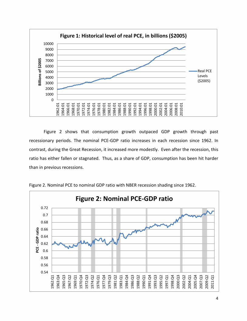
Figure 4 displays the time path of the real PCE growth rate for the 2008/2009 recession
around the NBER peak and compares it with the average real PCE growth rates from all other
recessions since 1971. This graph shows that the average real PCE growth rate around the
2008/2009 recession was significantly lower than the corresponding average over the previous
five recessions. Consumption has grown 4.1% in total over the last 5 years, or an average rate
of .8% per year. This is in contrast with the fact that over the 1971-present consumption
growth averaged 3.1% per year, adding up to about 15% growth over an average 5-year period.
Thus, consumption expenditures are about 15%-4%=11% below what they would have been
had they grown at their historical averages from 2007:Q4 onward.
Figure 4. Real total quarterly PCE growth over the 2008/2009 recession compared with the
average quarterly growth rates of all other previous recessions since 1974.
-6
-4
-2
0
2
4
6
-16 -14 -12 -10 -8 -6 -4 -2 0 2 4 6 8 10 12 14 16
Qua
rter
ly G
row
th (A
nnua
l Rat
e)
Quarters Since Peak
Figure 4: Real total PCE growth
Average of Previous Recessions
Q4-07

7
All sub-components of PCE fell during the Great Recession. Durables growth was
somewhat weaker than in the previous five recessionary periods, both in terms of average
growth rate and pattern of recovery. However, non-durables, and especially services, were the
sub-components that were most depressed compared to the previous recessions.
Total real PCE services
Figure 5 highlights that the behavior of PCE services was starkly different over the last
2008/2009 recession compared to all other recessions since 1974. In all other recessions PCE
services grew both before and after the peak, while during the last recession, it stagnated
starting 2 quarters after the peak (four quarters before the trough) and kept stagnating for four
additional quarters afterwards. It took until Q4 2010 to return to peak levels.
Figure 5. Spider chart comparing the time path of real PCE services over several recessionary
time periods. For each recession, the level of PCE services is normalized to 1 at the NBER peak
prior to the recession.
Regarding the main services subcomponents, Petev, Pistaferri, and Ecksten (2010)
document that spending on health services increased, held stable for housing and utilities, but
0.8
0.85
0.9
0.95
1
1.05
1.1
1.15
1.2
-16 -14 -12 -10 -8 -6 -4 -2 0 2 4 6 8 10 12 14 16
Peak
leve
l = 1
Quarters Since Peak
Figure 5: Normalized real PCE services levels over recession periods
Q4-73
Q1-80
Q3-81
Q3-90
Q1-01
Q4-07
8
declined substantially for services related to transportation, food and recreation. In sum, the
most adjustable services dropped, while those that the consumer has little flexibility about, did
not.
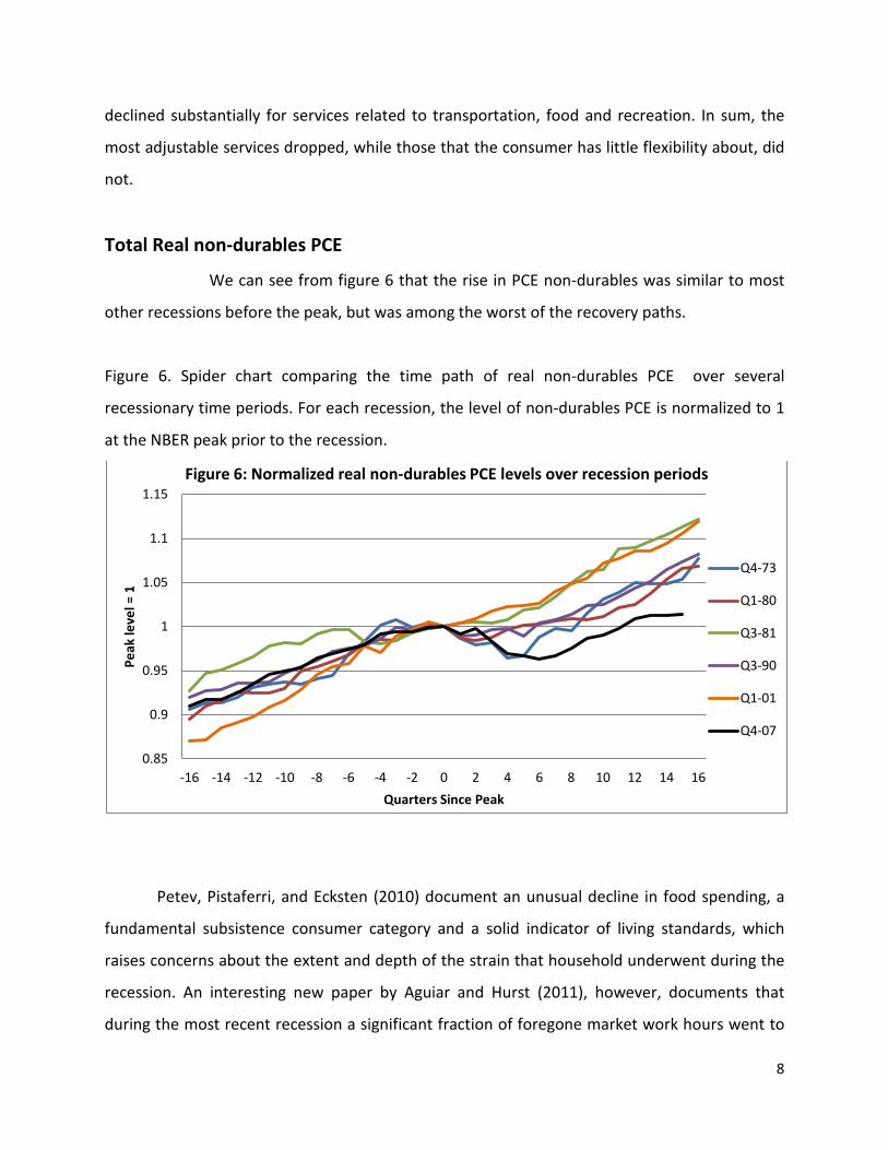
Total Real non-durables PCE
We can see from figure 6 that the rise in PCE non-durables was similar to most
other recessions before the peak, but was among the worst of the recovery paths.
Figure 6. Spider chart comparing the time path of real non-durables PCE over several
recessionary time periods. For each recession, the level of non-durables PCE is normalized to 1
at the NBER peak prior to the recession.
Petev, Pistaferri, and Ecksten (2010) document an unusual decline in food spending, a
fundamental subsistence consumer category and a solid indicator of living standards, which
raises concerns about the extent and depth of the strain that household underwent during the
recession. An interesting new paper by Aguiar and Hurst (2011), however, documents that
during the most recent recession a significant fraction of foregone market work hours went to
0.85
0.9
0.95
1
1.05
1.1
1.15
-16 -14 -12 -10 -8 -6 -4 -2 0 2 4 6 8 10 12 14 16
Peak
leve
l = 1
Quarters Since Peak
Figure 6: Normalized real non-durables PCE levels over recession periods
Q4-73
Q1-80
Q3-81
Q3-90
Q1-01
Q4-07
9
home production. Including childcare, that fraction of time is 35%. This is an important channel
that could produce more goods (such as food) and services (such as childcare) at a lower cost.
More work is needed to determine if home production could completely explain the observed
decline in food spending.
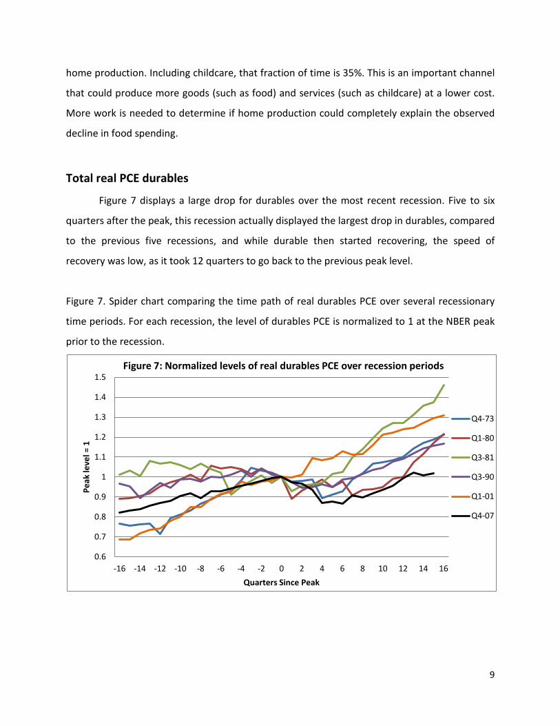
Total real PCE durables
Figure 7 displays a large drop for durables over the most recent recession. Five to six
quarters after the peak, this recession actually displayed the largest drop in durables, compared
to the previous five recessions, and while durable then started recovering, the speed of
recovery was low, as it took 12 quarters to go back to the previous peak level.
Figure 7. Spider chart comparing the time path of real durables PCE over several recessionary
time periods. For each recession, the level of durables PCE is normalized to 1 at the NBER peak
prior to the recession.
0.6
0.7
0.8
0.9
1
1.1
1.2
1.3
1.4
1.5
-16 -14 -12 -10 -8 -6 -4 -2 0 2 4 6 8 10 12 14 16
Peak
leve
l = 1
Quarters Since Peak
Figure 7: Normalized levels of real durables PCE over recession periods
Q4-73
Q1-80
Q3-81
Q3-90
Q1-01
Q4-07

10
Petev, Pistaferri, and Ecksten (2010) document that the bulk in the decline in real per-
capital spending is attributable to purchases of cars (a 25% decline by the end of 2008) and
partly of furniture (a 9% decline).
To summarize, our main findings from the macro data are as follows. First, the Great
Recession marked the most severe and persistent decline in aggregate consumption since
WWII. All subcomponents of consumption declined during this period. However, we find that
the significant drop in consumed services stands out most compared to previous recessions.
Second, while the decline was historic, the time path of consumption and its subcomponents
leading up the recession was not substantially different from past recessionary periods. Third,
the recovery path of consumption following the Great Recession has been uncharacteristically
weak. It took nearly three years for total consumption to return to its level just prior to the
recession. In contrast, the second worst rebound observed in the data followed the 1974
recession and was just over one year. We find that this persistence is reflected most in the
subcomponents of non-durables and especially services consumption.
The Micro evidence: expected income in the Michigan Survey of Consumers
This section documents consumer expectations for future income, both in nominal and real
terms, to see whether shocks to permanent income are contributing to the consumption dip.
The survey asks two questions to identify the magnitude and sign of the income change.
i) “During the next 12 months, do you expect your income to be higher or lower than
during the past year?”
ii) “By about what percent do you expect your income to (increase/decrease) during
the next 12 months?”
The resulting index of expected income growth ranges between +95 and -95 in the cross-
section and reflects the expected percent change in nominal income in the next year. The
historical mean is +5.5%, split between +4.8% during recessions and +5.6% during expansions.
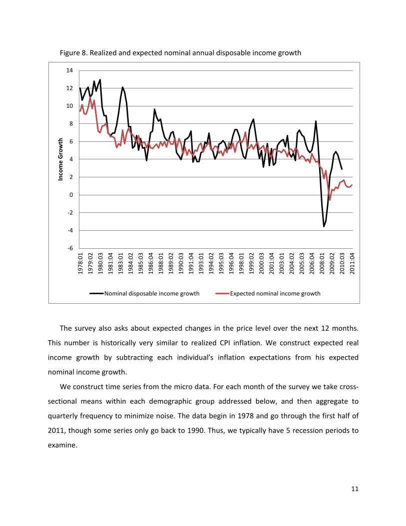
Figure 8 below compares realized and expected nominal disposable income and shows that the
two series track each other well.
11
Figure 8. Realized and expected nominal annual disposable income growth
The survey also asks about expected changes in the price level over the next 12 months.
This number is historically very similar to realized CPI inflation. We construct expected real
income growth by subtracting each individual's inflation expectations from his expected
nominal income growth.
We construct time series from the micro data. For each month of the survey we take cross-
sectional means within each demographic group addressed below, and then aggregate to
quarterly frequency to minimize noise. The data begin in 1978 and go through the first half of
2011, though some series only go back to 1990. Thus, we typically have 5 recession periods to
examine.
-6
-4
-2
0
2
4
6
8
10
12
14 19
78:0
1 19
79:0
2 19
80:0
3 19
81:0
4 19
83:0
1 19
84:0
2 19
85:0
3 19
86:0
4 19
88:0
1 19
89:0
2 19
90:0
3 19
91:0
4 19
93:0
1 19
94:0
2 19
95:0
3 19
96:0
4 19
98:0
1 19
99:0
2 20
00:0
3 20
01:0
4 20
03:0
1 20
04:0
2 20
05:0
3 20
06:0
4 20
08:0
1 20
09:0
2 20
10:0
3 20
11:0
4
Inco
me
Gro
wth
Nominal disposable income growth Expected nominal income growth

12
Nominal income growth expectations
Except for the Great Recession and the 1980 recession, income expectations show a
downward trend for up to four quarters around the NBER peak, but then stabilize and actually
rise by the end of our 4 year window (see figure 9). For both the 1980 and most recent
recession, we observe larger and more prolonged dips. Besides the abnormal drop, both in
terms of size and duration, the recovery periods also stand out for their length and
sluggishness. Even well after 10 quarters from the peak, expected nominal income growth was
still well below the pre-recessionary periods. In terms of levels, it should be noted that the most
recent recession is the only one during which nominal income expectations reached negative
growth rates. Along all of the previous recessions that we study, even when nominal income
growth rates go down, they stay well above 4%. Of course, inflation has been lower during the
most recent recession. We will discuss real income patterns later.
Figure 9. Average expected nominal income growth rates around recessionary periods.
-2
0
2
4
6
8
10
12
-16
-15
-14
-13
-12
-11
-10 -9
-8
-7
-6
-5
-4
-3
-2
-1
0 1 2 3 4 5 6 7 8 9 10
11
12
13
14
15
16
Expe
cted
nom
inal
inco
me
grow
th
Quarters since peak
Great Recession 2007:Q4 2001:Q1 1990:Q3 1981:Q3 1990:Q1

13
Figure 10 shows that after the late 1970s, nominal income growth expectations have
not varied by demographics until the most recent recession. Prime age individuals (30-59)
experienced the largest drop in expected nominal income growth during the Great Recession
and are only partially recovering even 10 quarters after the peak. For younger consumers,
expectations dropped well before, starting 5 quarters in advance, but then stabilized after the
peak.
Figure 10. Expected nominal income growth, by age group.
-5
0
5
10
15
20
-16 -12 -8 -4 0 4 8 12 16
Expe
cted
nom
inal
inco
me
grow
th
Quarters since peak 1981:Q3
-5
0
5
10
15
20
-16 -12 -8 -4 0 4 8 12 16 Quarters since peak 1990:Q3
-5
0
5
10
15
20
-16 -12 -8 -4 0 4 8 12 16
Expe
cted
nom
inal
inco
me
grow
th
Quarters since peak 2001:Q1
18-29 30-59 60-69 70+
-5
0
5
10
15
20
-16 -12 -8 -4 0 4 8 12 16 Quarters since peak 2007:Q4 - Great Recession
18-29 30-59 60-69 70+

14
In past recession periods, nominal income expectations of the elderly population
hovered around or just above zero. However, these expectations been markedly negative since
the NBER peak in 2007:Q4. Focusing on this population, Christelis, Georgarakos, and Jappelli
(2011) use the 2009 Internet Survey of Health and Retirement Study (HRS) to look at the effects
of three different shocks: the drop in house prices, the decline in the stock market, and the
increase in unemployment, on households’ expenditures during the Great Recession. This data
set refers to the population 50 and older. The HRS Internet Survey contains detailed measures
of both housing wealth losses (between Summer 2006 and Mid-2009) and of losses in various
financial assets (between October 2008 and Mid-2009). It also contains measures of
consumption growth and qualitative indicators of consumption changes, allowing them to
estimate the effect of the losses on adjustments in consumption expenditure. Their main
finding is that capital losses (on housing and financial assets), as well as the income loss from
becoming unemployed, lead households to reduce their spending. The estimated elasticity of
consumption to financial wealth implies a marginal propensity to consume with respect to
financial wealth equal to 3 percentage points. The decline in house prices also had an important
impact on consumption: the estimated elasticity implies that the marginal propensity to
consume is 1 percentage point. Additionally, households in which at least one of the two
partners in the main couple (or the single head) became unemployed in 2008 and early 2009
reduced consumption by 10% in 2009. See Hurd and Rohwedder (2010a, 2010b) and the
citations therein for more estimates on the responsiveness of consumption to asset and income
shocks.
Figure 11 shows that all income levels have adjusted their expected income growth
downward during the most recent recession. In past recessions the adjustments were smaller.
In the most recent recession, the 1st quintile (the poorest) dropped the least. By the end of
2010 all income levels have roughly converged to the same post-peak level and are much closer
together. This is consistent with Petev, Pistaferri, and Ecksten’s findings. First, they find that
increased government transfers propped up income among the poorest-income households
during the Great recession. Second, using the Michigan Index of Consumer Sentiment, they
document that high income people have become more pessimistic than other groups during

15
the Great Recession.2 Finally, using the Consumer Expenditure Survey (CEX), they find that
respondents in the top decile of the wealth distribution are the ones who decrease spending
during the Great Recession (-5.4%). This finding holds for the subcategories of nondurables and
services. This drop in consumption might be due to the large negative wealth effect
experienced by these households due to the decrease in house values and stock market
valuation.
Figure 11. Expected nominal income growth by income quintile.
2 As a possible explanation for the pessimism of the wealthy, Shapiro (2010) finds that these household were exposed more to the stock market and experienced larger declines in wealth as a consequence. The median decline in wealth was 15% in Shapiro’s data, and those who lost at least 10% of their net worth had almost twice the mean wealth and 3.5 times the median wealth of the sample.
-5
0
5
10
15
-16 -12 -8 -4 0 4 8 12 16
Expe
cted
nom
inal
inco
me
grow
th
Quarters since peak 1981:Q3
-5
0
5
10
15
-16 -12 -8 -4 0 4 8 12 16 Quarters since peak 1990:Q3
-5
0
5
10
15
-16 -12 -8 -4 0 4 8 12 16
Expe
cted
nom
inal
inco
me
grow
th
Quarters since peak 2001:Q1
1st quintile 2nd quintile
3rd quintile 4th quintile
5th quintile
-5
0
5
10
15
-16 -12 -8 -4 0 4 8 12 16 Quarters since peak 2007:Q4 - Great Recession
1st quintile 2nd quintile
3rd quintile 4th quintile
5th quintile

16
Figure 12 shows that in the previous recessions, income expectations by education
groups were rather flat over the cycle. In the most recent recession, everyone reduced their
expected income growth.
Figure 12. Expected nominal income growth by education level.
-5
0
5
10
15
-16 -12 -8 -4 0 4 8 12 16
Expe
cted
nom
inal
inco
me
grow
th
Quarters since peak 1981:Q3
-5
0
5
10
15
-16 -12 -8 -4 0 4 8 12 16 Quarters since peak 1990:Q3
-5
0
5
10
15
-16 -12 -8 -4 0 4 8 12 16
Expe
cted
nom
inal
inco
me
grow
th
Quarters since peak 2001:Q1
HS dropouts HS grads
Some college College+
-5
0
5
10
15
-16 -12 -8 -4 0 4 8 12 16 Quarters since peak 2007:Q4 - Great Recession
HS dropouts HS grads
Some college College+

17
Real income growth expectations.
Nominal income growth during the Great Recession was low, but inflation was also low.
To study the behavior of real income expectations, we measure inflation in two ways. First, we
use actual CPI inflation over the 12 month period covered by the survey question, which
assumes that consumers have perfect foresight over the next year concerning inflation. Second,
we use the answer to the survey question about the individual’s expectation about growth in
prices over the next 12 months. Using these two measures, we construct individual-level
expected real income growth and then aggregate up to population-quarter means.
The two inflation series have diverged in the past, but after the late 70s the differences
are minor. At the start of the Great Recession, however, a large gap opened up, which makes
for the largest discrepancy between these two data series. The swing in 2008 Q2 is +6% in
expected inflation, compared to -1% actual CPI inflation. The two measures have since become
closer together (see figure 13). The gap in these two measures of course impacts measured real
income growth expectations as we document below.
Figure 13. Time series of 12 months forward inflation since 1978, comparing CPI and personal
inflation expectations for the Michigan Survey of Consumers.
-4
-2
0
2
4
6
8
10
12
14
16
1978
:01
1979
:02
1980
:03
1981
:04
1983
:01
1984
:02
1985
:03
1986
:04
1988
:01
1989
:02
1990
:03
1991
:04
1993
:01
1994
:02
1995
:03
1996
:04
1998
:01
1999
:02
2000
:03
2001
:04
2003
:01
2004
:02
2005
:03
2006
:04
2008
:01
2009
:02
2010
:03
2011
:04
Year
-ove
r-ye
ar in
flatio
n
CPI inflation Consumer expected inflation

18
In figure 14 there is no clear cyclical pattern prior to the Great Recession in real income
expectations. Before the most recent recession, real income growth was rather flat, dropped
into negative territory several quarters before the peak, but then went up to about 4% four
quarters after the peak. From then on, however, it had a large drop, reaching -3% five quarters
after the peak. In summary, real income growth expectations deflated by CPI show a
deterioration and lower average growth than during previous recessions.
Figure 14. Expected real income growth, CPI inflation.
Figure 15 shows that perceived consumers’ real income growth using the consumers’
inflation expectactions provides a much more pessimistic outlook about consumers’ purchasing
power during the Great Recession. Consumers’ perceived real income growth dipped in and out
of negative territory well before the recession started, and sustained a large drop starting four
-6
-4
-2
0
2
4
6
-16
-15
-14
-13
-12
-11
-10 -9
-8
-7
-6
-5
-4
-3
-2
-1
0 1 2 3 4 5 6 7 8 9 10
11
12
13
14
15
16
Expe
cted
real
inco
me
grow
th (C
PI in
flatio
n)
Quarters since peak
Great Recession 2007:Q4 2001:Q1 1990:Q3 1981:Q3 1980:Q1

19
quarters before the peak. That drop brought expectations from almost +2% to -4% growth rate
three quarters after the peak. It took two more quarters to go back up to a -2% growth rate
expectation, but there has been stagnation ever since. The recession window in figure 15 ends
in Q4 2011 at an expected real income growth of -2.5%. In 2011 the series has recorded values
of -3.1%, -3.7%, and -2.9% for quarters 1 through 3, respectively.
Figure 15. Expected real income growth, using consumers’ inflation expectations.
Our main findings from the analysis of the Micro data are as follows. First, expected nominal
income growth declined significantly during the Great Recession. It is the worst drop ever
observed in these data, and it has not recovered to pre-recession levels. Second, the decline
exists for all age groups, education levels, and income quintiles. Relative to previous
recessions, those with higher levels of income and education are more pessimistic than their
poorer and less educated counterparts. Third, expectations for real income growth have also
-6
-4
-2
0
2
4
6
-16
-15
-14
-13
-12
-11
-10 -9
-8
-7
-6
-5
-4
-3
-2
-1
0 1 2 3 4 5 6 7 8 9 10
11
12
13
14
15
16
Expe
cted
real
inco
me
grow
th (p
erso
nal i
nfla
tion
expe
ctat
ions
)
Quarters since peak
Great Recession 2007:Q4 2001:Q1 1990:Q3 1981:Q3 1980:Q1

20
declined, and the decline in expected real income growth is more severe when personal
inflation expectations are used instead of actual CPI inflation.
Does the Michigan Expectations data have predictive power for future income
and consumption growth?
Below we show that the Michigan data have a great deal of forecasting power for both
future disposable income and consumption growth.3 We estimate the regression for
disposable income first:
4 0 1 4 4 2(( ) / ) (( ) / )t k t k t k t t t Mt t kY Y Y Y Y Y gα α α ε+ + + + − − +− = + − + +
where 0α , 1α , 2α are parameters to estimate and 1α and 2α are reported in the table below.
The variable 4(( ) / )t k t k t kY Y Y+ + + +− is next year’s annual income growth k quarters from now, so
k is 0 when forecasting income growth over the next year and 4 when forecasting income
growth over the subsequent year. 4 4(( ) / )t t tY Y Y− −− is income growth over the last year and
Mtg is expected real income growth from the Michigan survey, where we deflate using
expected inflation from the Michigan survey.
As can be seen in table 1, lagged income growth has a negative coefficient and expected
income growth has a positive coefficient. For income growth over the next year the coefficient
on expected income growth is .80, indicating that a 1% decline in expected income growth
reduces next year’s income growth .80%, controlling for last year’s income growth. The right
hand column shows that predicted income growth over the next year (2011:Q3 to 2012:Q3)
using lagged income growth and expected income growth is .6%, well below its average of 2.8%
over the 1978-2011 sample period. Income growth between 2012:Q3 and 2013:Q3 is also
forecasted to be low.
3 See Souleles (2004), Ludvigson (2004), and Barsky and Sims (2009) for more on the predictive power of the Michigan surveys.

21
Expected income growth is also a good predictor of consumption growth. Table 1 also
presents regressions using future consumption growth as the left hand side variable and lagged
consumption growth and the Michigan expectations variable as the right hand side variables.
The consumption forecast for 2011:Q3 to 2012:Q3 is for 0.1% growth.
In short, the low expected income growth in the Michigan Consumer Survey data
suggest that the US will experience low income and consumption growth over the next two
years. Obviously, there are many things not in our models so the estimates should only be
taken as suggestive evidence. However, the results are fairly robust to changes in model
specification and adding a few other variables, such as the unemployment rate.
Table 1: Regression Results
Lagged income Michigan
Lagged consumption
Forecasted annual
Dependent variable growth variable
income expectations
growth variable
growth, Q3/Q3 R-squared
Annual income growth 1 year forward
-0.35 0.80 -- 0.61* 0.29 (0.10) (0.17)
Annual income growth 2 years forward
0.06 0.36 -- 1.24** 0.08 (0.08) (0.17)
Annual income growth 3 years forward
-0.34 0.42 -- 2.16*** 0.08 (0.13) (0.20)
Annual consumption growth 1 year forward
-- 0.71 0.08 0.05* 0.37
(0.23) (0.13) Annual consumption growth 2 years forward
-- 0.77 -0.25 0.13** 0.18
(0.23) (0.16) Annual consumption growth 3 years forward
-- 0.58 -0.49 1.15*** 0.11
(0.27) (0.19) Annual consumption growth 1 year forward
-0.20 0.75 0.18 0.39* 0.39 (0.14) (0.21) (0.14)
Annual consumption growth 2 years forward
0.10 0.76 -0.31 -0.07** 0.17 (0.14) (0.23) (0.19)
Annual consumption growth 3 years forward
-0.09 0.59 -0.44 1.36*** 0.11 (0.16) (0.27) (0.21)
Notes: Regressions are run with data from 1978:Q1 to 2011:Q2. Newey-West standard errors in parentheses. Average annual income and consumption growth are 2.78 and 2.91, respectively. Using data up to 2011:Q3, forecast of growth between: *2011:Q3 and 2012:Q3 **2012:Q3 and 2013:Q3

22
***2013:Q3 and 2014:Q3
Using a simple model to quantify the effects of the drops in wealth and income
expectations
Data from the Federal Reserve Board of Governors’ Flow of Funds shows that in 2008
American households experienced a loss of $13.6 trillion in wealth, with most of the loss
concentrated in stock market wealth. Although stock market wealth partially recovered since
then, housing wealth has continued to decline. The resulting wealth loss, combined with lower
expected income growth, has the potential to explain why the consumers cut back
consumption during the Great Recession to the extent that they did. We turn to quantifying the effects of these declines by first calibrating a simple model of
consumption that matches the observed level of consumption in 2007:Q4, and that implies
empirically plausible marginal propensities to consume (MPCs) out of assets and permanent
income. Then, we show model predicted consumption in 2011:Q2 under different expectations
for income and asset values. We find that for reasonable parameter values, the decline in
assets can explain 1/3 of the gap between actual and potential consumption, while declines in
permanent income expectations can easily explain the other 2/3 of the gap.
Figure 16 Real Consumption Expenditures with and without the Great Recession

23
Model
Define tC as consumption expenditures at time t (where time is measured in quarters).
Households maximize
1) 0
ln( )tt
t tC
∞
=
β∑
subject to the following asset accumulation equation,
2) 1 1(1 ) 0t t t t TA r A Y C A+ += + + − , ≥
0tA given, and given income expectations. To avoid the additional complication of dealing with
uncertainty, we assume that individuals are certain of future income. However, we allow them to revise
their perceived income process if they make a mistake.
The solution to the consumer’s problem is:
3) (1 )( )t t tC Y A= −β +
where
8900
9200
9500
9800
10100
10400
10700
2006
:01
2006
:02
2006
:03
2006
:04
2007
:01
2007
:02
2007
:03
2007
:04
2008
:01
2008
:02
2008
:03
2008
:04
2009
:01
2009
:02
2009
:03
2009
:04
2010
:01
2010
:02
2010
:03
2010
:04
2011
:01
2011
:02
2011
:03
2011
:04
Billi
ons $
2005
PCE Counter-factual PCE

24
4) (1 (1 )) tt
tY r Y
∞τ−
ττ=
= / +∑
is the present value of future labor income.
We compute tY by assuming that consumers observe income up to 2011:Q2 and that from that
point on, income expectations for the next year are those measured in the most recent Michigan Survey
of Consumers, but then revert to long run income growth afterwards.
Mathematically, we can write this as
Yt+k = (1+gM)kYt, k ≤ 4
Yt+k = (1+g)Yt+k−1, k > 4
where Yt is disposable income, gM is the perceived real income growth for the next year in the 2010:Q4
(the most recent release of this variable suggests even more pessimism on consumer’s part than in
2010:Q4) Michigan Survey of Consumers, while g is the average growth rate of income over the last 40
years. Putting these equations together yields
5)
2
3 4
2
2
(1 )3 4( )
(1 (1 ))
(1 (1 ) (1 ) ((1 ) (1 ))
((1 ) (1 )) ((1 ) (1 ))
[1 (1 ) (1 ) ((1 ) (1 )) ]
(1 (1 ) (1 ) ((1 ) (1 ))
((1 ) (1 )) ((1 ) (1 ))
tt t
t M M
M M
t M M
rM M r g
Y r Y
Y g r g r
g r g r
g r g r
Y g r g r
g r g r
∞ τ−ττ=
+−
= / +
= + + / + + + / +
+ + / + + + / +
× + + / + + + / + + ...
= + + / + + + / +
+ + / + + + / +
∑
).
We call the income process above income process 1. Then, to show the importance of low
expected income growth, we consider a more pessimistic scenario, which we call income process 2, in
which rather than reverting back to a long-run expected growth after four quarters, pessimism about
income growth persists on forever. When this is the case,

25
6) (1 )
( )
(1 (1 ))
( )M
tt t
rt r g
Y r Y
Y
∞ τ−ττ=
+−
= / +
= .
∑
Figure 17 reports four different lines for the time path of real disposable income since the
beginning of 2007. The top crossed line shows counterfactual disposable income level, had it continued
to grow at its historical average rate of 3.2% from 2007:Q4 on. The triangle line shows realized
disposable income up to 2011:Q2. The dashed line begins with realized disposable income in 2011:Q2. It
then tacks on the expected level of disposable income using expectation data from the Michigan Survey
of Consumers for all periods thereafter. This corresponds to income process 2. The dotted line begins in
2012:Q2, assuming that income grows according to the Michigan Survey of Consumers between
2011:Q2 and 2012:Q4, and then grows at its historical rate afterwards. It corresponds to income process
1.
Figure 17. Disposable income and assumed income processes

26
Calibration
The three key moments we wish to match are the marginal propensity to consume (MPC) out of
assets, the MPC out of permanent income, and the level of consumption in 2007:Q4.
Most estimates of the MPC out of assets are around .01-.05 and most estimates of the MPC out
of permanent income are around .5-1. We assume the MPC out of assets is .03 per year. We use per
capita income growth for the individual’s decision problem. Thus we set 032 014 018g = . − . = .
(average disposable income growth over the 1967:4 to 2007:4 period less population growth of those
age 16+ over the same time period). We pick r and β to match the MPC out of assets and the level of
consumption in 2007:Q4. Thus we match
(1 ) 03t
t
CA
∂= −β = .
∂
9500
9900
10300
10700
11100
11500
2006
:01
2006
:02
2006
:03
2006
:04
2007
:01
2007
:02
2007
:03
2007
:04
2008
:01
2008
:02
2008
:03
2008
:04
2009
:01
2009
:02
2009
:03
2009
:04
2010
:01
2010
:02
2010
:03
2010
:04
2011
:01
2011
:02
2011
:03
2011
:04
2012
:01
2012
:02
2012
:03
2012
:04
Billi
ons $
2005
Disposable income Counter-factual disposable income
Income process 1 Income process 2

27
2007 4 2007 4 2007 41(1 )[ ]Q Q Q
rC Y Ar g: : :
+= −β +
−
Where C2007:Q4 = $9,312.6 billion (at an annualized rate), Y2007:Q4 = $9,944 billion (annualized), and A2007:Q4
= $69,139 billion.
The unit of time in this analysis is a quarter, although so far we have been discussing all
calibrations at annualized rates. We convert annual growth rates to quarterly ones, using the formula
(1/4)(1 ) 1g+ − when taking the quarterly growth rate for g. For dollar amounts, we divide by 4. After
converting everything to quarterly rates, we use the above two equations to solve for β and r. Table 1
presents all variables at quarterly and annualized rates. At annualized rates, β = .97 and
r=.060.This gives a quarterly MPC out of permanent income equal to
(1 )[(1 ) ( )] 730t
t
C r r gY
∂= −β + / − = .
∂
which is consistent with the evidence in the literature.
Over the last 40 years annual population growth for those aged 16+ is 1.4%, which we define as
p. We assume this rate of population growth continues on into the future. Income growth in the
individual’s decision problem is in per capita terms. We then account for aggregate growth at the end by
adjusting up disposable income by 1.4% at an annual rate.
Table 1: Model Parameters Annual Quarterly Exogenously set
-0.016 -0.0040 Population growth 0.014 0.0035 g 0.018 0.0045 MPC out of assets 0.03 0.0074
Mg

28
Y2007:Q4 9,944 2486
C2007:Q5 9,313 2,328
A2007:Q4 69,139 69,139 Endogenously determined
β 0.97 0.993 r 0.060 0.015 Implied MPC out of income
0.730
Results
Table 2 explains our key findings. All quarterly numbers in this section are annualized; i.e., they are the
quarterly numbers multiplied by 4. Consumption expenditures in 2011:Q2 were $9.379 trillion. Had
they grown at average rates from 2007:Q4 on, they would have been at $10.472 trillion in 2011:Q2,
which is 10% higher than it is today. This difference of $1.069 trillion, line 3 of the table, is the shortfall
we seek to explain with the model. Figure 16 depicts this shortfall graphically.
Table 2: Results Realized consumption level 2011:Q2 9379
Predicted consumption level 2011:Q2 given information in 2007:Q4 10472 Consumption loss 1093
Consumption loss due to asset value decline Asset value decline 9746
Predicted consumption decline due to asset price decline 289 Consumption loss given disposable income decline
Income process 1 917 Income process 1 and lower short-term interest rate 710
Income process 2 4038 Consumption loss given both asset and income declines
Income process 1 1206 Income process 1 and lower short-term interest rate 999
Income process 2 4328 Note: All amounts in Billions of dollars
Lines 5 and 6 in Table 2 study the effects of the decline in asset prices. Net worth fell $9.746 trillion in
real terms over this time period. Given a quarterly MPC of .0074, we predict a ($9.746 trillion)X(.0074)X4
= $.289 trillion fall in consumption, at an annualized rate.

29
The following lines in the table predict the consumption fall due to various permanent income
scenarios. To perform this computation, we first put ourselves in 2007:Q4 and predict Y as of 2011:Q2,
had income grown steadily at its long-run historical average. Second, we calculateY given realized
income in 2007:Q4 and the two income processes that we have described previously. To be clear, taking
into account population growth rates, we calculate 2011 2QY : , given information set from 2007:Q4 =
1412007 4 2007 4 ((1 )(1 ))r
Q Q r gY Y p g+: : −= + + , where 14 is the number of quarters between 2007:Q2 and
2011:Q4.
Once we calculate the loss in Y under different income and interest rate scenarios, we use the
model to calculate the resulting consumption loss. The consumption loss associated with income
process 1 is $0.917 trillion, which is reasonably close to the observed consumption loss. This
computation is sensitive to the time path of the interest rate as well. The baseline calibration yields a
yearly interest rate of 6%. In the lower short term interest rate scenario we assume that over the first
year the yearly interest rate is 3% and then reverts back to 6%. In this case, income is less heavily
discounted, hence its present value is higher and the implied consumption drop is $710 billion rather
than $917 billion. Unsurprisingly, the very pessimistic income expectation scenario considered in Income
process 2, generates a huge consumption loss of $4.038 trillion, which is almost 4 times larger than the
consumption shortfall we wish to explain.
Because our model predicts that consumption is linear in resources (assets and the present
value of future income), we can add up losses from assets and income. Note that the predicted
consumption decline given the asset fall plus the predicted decline given income process 1 of $1.206
trillion lines up almost exactly with what is in the data.

30
Conclusions
This article documents key facts about aggregate consumption and its subcomponents
and looks at the behavior of important determinants of consumption over the cycle, such as
consumption is consumer’s expectations about their future income, and changes in the
consumers’ wealth positions due to changes in house prices and stock valuation. We performed
a simple computation to determine whether the observed drop in consumption can be
explained by the observed drops in wealth and income expectations.
In the context of a simple permanent income model, we find that the negative wealth
effect (coming from decreased stock market valuation and housing prices) and decreased
consumer’s income expectations were big factors in determining the observed consumption
drop. In fact, we find that in this model the observed drops in wealth and income expectations
can explain the observed drop in consumption in its entirety, depending on what is assumed
about future income growth going forward, beyond the time horizon covered by the Michigan
Survey of Consumers data set.

31
Bibliography
Aguiar Mark, and Eric Hurst, 2011 “Time Use During Recessions.” NBER WP. 17259.
Barsky, Robert, and Eric Sims, 2009. “Information, animal spirits, and the meaning of
innovations in consumer confidence.” NBER wp 15049.
Christelis Dimitris, Dimitris Georgarakos, and Tullio Jappelli, 2011 “Wealth Shocks,
Unemployment Shocks and Consumption in the Wake of the Great Recession.”
Hurd Michael and Susan Rowwedder, 2010a “The Effects of the Economic Crisis on the Older
Population,” MRRC WP 2010-231.
Hurd Michael and Susan Rowwedder, 2010b “Effects of the Financial Crisis and Great Recession
on American Households,” NBER wp 16407.
Petev Ivalyo, Luigi Pistaferri, and Itay Eksten, 2010 “Consumption and the Great Recession: An
Analysis of Trends, Perceptions, and Distributional Effects.” Mimeo, Stanford University.
Shapiro Matt, 2010 “The Effects of the Financial crisis on the Well-being of Older Americans:
Evidence from the Cognitive Economic Study,” MRRC WP 2010-228.
Souleles, Nicholas, 2004. “Expectations, heterogeneous forecast errors, and consumperion:
Micro evidence from the Michigan Consumer Sentiment Surveys.” Journal of Money, Credit and
Banking. 36(1), February.