consumption access and the spatial concentration of
TRANSCRIPT
Consumption Access and the Spatial Concentrationof Economic Activity: Evidence from
Smartphone Data∗
Yuhei Miyauchi†
Boston University
Kentaro Nakajima‡
Hitotsubashi University
Stephen J. Redding§
Princeton University, NBER and CEPR
June 3, 2021
Abstract
Using smartphone data for Japan, we show that non-commuting trips are frequent, morelocalized than commuting trips, strongly related to the availability of nontraded services,and occur along trip chains. Guided by these empirical findings, we develop a quantitativeurban model that incorporates travel to work and travel to consume non-traded services.We use the gravity equation predictions of the model to estimate theoretically-consistentmeasures of travel access. We show that consumption access makes a substantial contribu-tion to the observed variation in residents and land prices and the observed impact of theopening of a new subway line.
Keywords: Cities, Consumption Access, Economic Geography, TransportationJEL Classification: O18, R12, R40
∗Thanks to Gabriel Ahlfeldt, Daniel Sturm and Gabriel Kreindler and conference and seminar participants forhelpful comments. We are grateful to Takeshi Fukasawa and Peter Deffebach for excellent research assistance.The usual disclaimer applies. “Konzatsu-Tokei (R)” Data refers to people flow data constructed from individuallocation information sent from mobile phones under users’ consent, through applications provided by NTT DO-COMO, INC (including mapping application Docomo Chizu NAVI). Those data are processed collectively andstatistically in order to conceal private information. Original location data is GPS data (latitude, longitude) sentevery five minutes, and it and does not include information to specify individual. The copyrights of all tables andfigures presented in this document belong to ZENRIN DataCom CO., LTD. We also acknowledge Yaichi Aoshimaat Hitotsubashi University for coordinating the project with ZENRIN DataCom Co,. LTD.; Heiwa Nakajima Foun-dation and The Kajima Foundation for their financial support; CSIS at the University of Tokyo for the joint researchsupport (Project No. 954); the Ministry of Land, Infrastructure, Transport, and Tourism and the Miyagi Prefecturefor the access to the travel survey data.†Dept. Economics, 270 Bay State Road, Boston, MA 02215. Tel: 1-617-353-5682. Email: [email protected].‡Institute of Innovation Research, 2-1 Naka, Kunitachi, Tokyo 186-8603, Japan. Tel: 81-42-580-8417. E-mail:
[email protected]§Dept. Economics and SPIA, JRR Building, Princeton, NJ 08544. Tel: 1-609-258-4016. Email: red-
1
1 Introduction
Understanding the spatial concentration of economic activity is one of the most central chal-lenges in economics. Traditional theories of cities emphasize production decisions and thecosts of workers commuting between their workplace and residence. However, much of thetravel that occurs within urban areas is related not to commuting but rather to the consump-tion of nontraded services, such as trips to restaurants, coffee shops and bars, shopping centers,cultural venues, and other services. Although several scholars have emphasized the “consumercity,” two major challenges in this area are a limited ability to measure non-commuting tripsand the absence of a widely-accepted theoretical model of travel for consumption. In this paper,we provide new theory and evidence on the role of consumption and workplace access in under-standing the spatial distribution of economic activity. We combine smartphone data includinghigh-frequency location information with spatially-disaggregated census data to measure com-muting and non-commuting trips within the Greater Tokyo metropolitan area. Guided by ourempirical findings, we develop a quantitative urban model that incorporates both workplace andconsumption access. We use the model to evaluate the role of consumption access in explainingthe observed spatial variation in economic activity. We show that incorporating consumptionaccess is quantitatively relevant for evaluating the observed impact of a new subway line.
We first use our smartphone data to provide fine resolution evidence on travel within theGreater Tokyo metropolitan area. Our data come from a major smartphone mapping applica-tion in Japan (Docomo Chizu NAVI), which records the Geographical Positioning System (GPS)location of each device every 5 minutes. In July of 2019, the data covers about 545,000 users,with 1.4 billion data points. We measure each location visited by a user using a “stay,” whichcorresponds to no movement within 100 meters for 15 minutes. We designate each anonymizeduser’s home location as her most frequent location (defined by groups of geographically con-tiguous stays) and her work location as her second most frequent location. We allocate non-commuting trips to other locations into different types using spatially-disaggregated census dataon employment by sector. We validate our smartphone commuting measures by showing thatthey are highly correlated with the measures from the official census data.
Having validated our smartphone data, we show that focusing solely on these commutingtrips provides a misleading picture of travel patterns. First, we show that non-commuting tripsare more frequent than commuting trips, so that concentrating solely on commuting trips sub-stantially underestimates the amount of travel within urban areas. Second, we show that thesenon-commuting trips are closely related to the availability of nontraded services, which is con-sistent with our modelling of them as travel to consume non-traded services. Third, we findthat non-commuting trips have destinations closer to home than commuting trips, with semi-
2
elasticities of travel flows to travel times that are larger in absolute value than those for com-muting trips. Therefore, the spatial patterns of non-commuting trips are not well approximatedby those for commuting trips. Fourth, we show that trip chains are a relevant feature of the data,in which non-commuting trips occur along the journey between home and work, highlightingthe relevance of jointly modelling commuting and non-commuting trips.
We next develop quantitative theory of internal city structure that incorporates both com-muting and consumption trips. We consider a city that consists of a discrete set of blocks thatdiffer in productivity, amenities, supply of floor space and transport connections. Consumerpreferences are defined over consumption of a traded good, a number of different types ofnontraded services, and residential floor space. The traded good and nontraded services areproduced using labor and commercial floor space. We assume that workers’ location decisionsare nested. First, workers observe idiosyncratic preferences for amenities in each location andchoose where to live. Second, workers observe idiosyncratic productivities in each workplaceand sector, and choose where to work. Third, workers observe idiosyncratic qualities for thenon-traded services supplied by each location, and choose where to consume these non-tradedservices. Fourth, workers observe idiosyncratic taste shocks for each route to consume thesenon-traded services, and choose which of these routes to take (e.g. home-work-consume-homeversus home-consume-home). When making each of these choices, workers take into accounttheir expected access to surrounding locations. Population mobility implies that workers mustobtain the same expected utility from all populated locations.
We show that the model implies extended gravity equations for commuting and non-commutingtrips, which provide good approximations to the observed data. We use these extended gravityequations to estimate a theoretically-consistent measure of travel access. Intuitively, we use theobserved trips in the data and the structure of the model to reveal the relative attractiveness oflocations for employment and consumption. From the model’s population mobility condition,we derive a sufficient statistic for the relative attractiveness of locations, which incorporatesboth the residential population share and the price of floor space. We show that this sufficientstatistic for the relative attractiveness of locations can be decomposed into our measure of travelaccess and a residual for residential amenities. Comparing our model incorporating both con-sumption and workplace access to a special case capturing only workplace access, we find asubstantially larger contribution of travel access once we take into account consumption access(56 percent compared to 37 percent), and a correspondingly smaller contribution from the resid-ual of residential amenities (44 percent compared to 63 percent). Taken together, this patternof results is consistent with the idea that much economic activity in urban areas is concentratedin the service sector, and that access to surrounding locations to consume these services is animportant determinant of workers’ choice of residence and workplace.
3

We show how the model can be used to undertake a counterfactual for a transport infras-tructure improvement, such as the construction of a new subway line. In addition to the initialshares of commuting trips, the predictions of these counterfactuals now also depend on the ini-tial shares of non-commuting trips. As a result, frameworks that focus solely on commutingtrips generally underestimate the welfare gains from transport infrastructure improvements, be-cause they undercount the number of passenger journeys that benefit from the reduction in travelcosts. Furthermore, these frameworks generate different predictions for the impact of the newtransport infrastructure on the spatial distribution of economic activity, because of the differentbilateral patterns of commuting and non-commuting trips. We compare the model’s counterfac-tual predictions for the opening of a new subway line to the estimated impact in the observeddata. We show that the model has predictive power for the observed data. We show that under-counting of travel from focusing on commuting trips leads to a substantial underestimate of thewelfare gains from the new subway line.
Our paper is related to a number of different strands of research. First, our findings re-late to recent research on endogenous amenities and social and spatial frictions within urbanareas. Evidence of endogenous amenities has been provided in the context of spatial sort-ing (Diamond 2016, Almagro and Domınguez-Iino 2019 and Samuels, Hausman, Cohen, andSasson 2016), gentrification and neighborhood change within cities (Glaeser, Kolko, and Saiz2001, Couture, Dingel, Green, and Handbury 2019, Hoelzlein 2020 and Allen, Fuchs, Gana-pati, Graziano, Madera, and Montoriol-Garriga 2020), and industry clustering (Leonardi andMoretti 2019). Evidence that both spatial and social frictions matter for agents’ location deci-sions has been provided using restaurant choice data (Couture 2016, Davis, Dingel, Monras, andMorales 2019), credit card data (Agarwal, Jensen, and Monte 2020 and Dolfen, Einav, Klenow,Klopack, Levin, Levin, and Best 2019), travel surveys and ride sharing data (Gorback 2020 andZarate 2020) and cellphone data (Couture, Dingel, Green, and Handbury 2019, Athey, Fergu-son, Gentzkow, and Schmidt 2018, Kreindler and Miyauchi 2019, Gupta, Kontokosta, and VanNieuwerburgh 2020, Buchel, Ehrlich, Puga, and Viladecans 2020 and Atkin, Chen, and Popov2021). Relative to these existing studies, we provide high-frequency and spatially-disaggregateddata on non-commuting trips, and develop a quantitative urban model for estimating workplaceand consumption access.
Second, our work contributes to research on transport infrastructure and the location ofeconomic activity. One strand of empirical research has used quasi-experimental variation onthe impact of transport infrastructure improvements, including Baum-Snow (2007), Michaels(2008), Duranton and Turner (2012), Faber (2014), and Storeygard (2016). A second line ofwork has used quantitative spatial models to evaluate general equilibrium impacts of transportinfrastructure investments, including Anas and Liu (2007), Donaldson (2018), Donaldson and
4
Hornbeck (2016), Heblich, Redding, and Sturm (2020), Tsivanidis (2018), Severen (2019),Balboni (2019), and Zarate (2020). While existing research emphasizes the costs of transportinggoods and commuting costs, a key feature of our work is to highlight the role of the transportnetwork in providing access to consume nontraded services.
Third, our research is related to recent research on the internal structure of cities, includingincluding Ahlfeldt, Redding, Sturm, and Wolf (2015), Allen, Arkolakis, and Li (2017), Monte,Redding, and Rossi-Hansberg (2018), Tsivanidis (2018), and Dingel and Tintelnot (2020). Allof these studies emphasize commuting and the separation of workplace and residence. In con-trast, one of our main contributions is to highlight the importance of travel to consume nontradedservices in shaping agents’ location decisions.
The remainder of the paper is structured as follows. Section 2 introduces our data. Section 3presents reduced-form evidence on travel patterns. Section 4 introduces our theoretical frame-work that we use to rationalize these findings. Section 5 uses the model to the quantify the rel-ative importance of consumption and workplace access for explaining the spatial concentrationof economic activity. Section 6 shows that incorporating consumption access is quantitativelyrelevant for evaluating the counterfactual impact of transport infrastructure improvements, suchas the construction of a new subway line. Section 7 concludes.
2 Data Description
In this section, we introduce our smartphone data and the other data used in the quantitativeanalysis of the model. In Subsection 2.1, we explain how we use our smartphone data to identifyhome location, work location, commuting trips and non-commuting trips. In Subsection 2.2,we discuss the spatially-disaggregated economic census data by sector and location that we useto distinguish between different types of non-commuting trips, and discuss our data on landvalues and other location characteristics. In Subsection 2.3, we report validation checks of thecommuting measures from our smartphone data using official census data on employment byresidence, employment by workplace and bilateral commuting flows.
2.1 Smartphone GPS Data
Our main data source is one of the leading smartphone mapping applications in Japan: Do-
como Chizu NAVI. Upon installing this application, individuals are asked to give permissionto share location information in an anonymized form. Conditional on this permission beinggiven, the application collects the Geographical Positioning System (GPS) coordinates of eachsmartphone device every 5 minutes whenever the device is turned on (regardless of whether theapplication is being used). These “big data” provide an immense volume of high-frequency and
5
spatially-disaggregated information on the geographical movements of users throughout eachday. For example for the month of July 2019 alone, the data include 1.4 billion data points on545,000 users (about 0.5 percent of the Japanese population).1
The raw unstructured geo-coordinates are pre-processed by the cell phone operator: NTTDocomo Inc. to construct measures of “stays,” which correspond to distinct geographical loca-tions visited by a user during a day. In particular, a stay corresponds to the set of geo-coordinatesof a given user that are contiguous in time, whose first and last data points are more than 15minutes apart, and whose geo-coordinates are all within 100 meters from the centroid of thesepoints.2 We have data on the sequence of stays of anonymized users with the necessary level ofspatial aggregation to deidentify individuals. Our data comprise a randomly selected sample of80 percent of users in Japan, where the randomization is again to deidentify individuals.
This pre-processing also categorizes all stays in each month into three categories of home,work and other locations for each anonymized user. “Home” location and “work” locationsare defined as the centroid of the first and second most frequent locations of geographicallycontiguous stays, respectively. To ensure that these two locations do not correspond to differentparts of a single property, we also require that the “work” location is more than 600 metersaway from the “home” location. In particular, if the second most frequent location is within600 meters of the “home” locations, we define the “work” location as the third most frequentlocation. To abstract from noise in geo-coordinate assignment, all stays within 500 meters of thehome location are aggregated with the home location. Similarly, all stays within 500 meters ofthe work location are aggregated with the work location. We assign “Work” location as missingif the user appears in that location for less than 5 days per month, which applies for about 30percent of users in our baseline sample during April 2019. These users primarily include thosewith limited number of data observations due to infrequent smartphone use, and also includeirregular workers with unstable job locations and those who work at home.3 In Subsection2.3 below, we report validation checks on our classification of home and work locations usingcommuting data from the population census. Stays which are neither assigned as home or workare classified as “other.” We distinguish between different types of these “other” stays, suchas visits to restaurants and stores, using spatially-disaggregated data on economic activity bysector and location from the economic census, as discussed further in Section 2.2 below.
1The mapping application does not send location data points if the smartphone does not sense movement, inwhich case it is likely that the user has not moved from the last reported location. For this reason, the data pointsare less frequent than 5 minutes intervals in practice.
2See Patent Number “JP 2013-89173 A” and “JP 2013-210969 A 2013.10.10” for the detailed proprietaryalgorithm. This algorithm involves processes to offset the potential noise in measuring GPS coordinates.
3In Section A.4 of our online appendix, we show that the devices with missing “work” locations have signifi-cantly fewer number of active days (even at home locations), and that the probability of assigning missing “work”locations is uncorrelated with the observable characteristics of the municipality of residence.
6
For most of our subsequent analysis, we focus on the sample of users in the month of April2019 who have home and work locations in the Tokyo Metropolitan Area (which includes thefour prefectures of Tokyo, Chiba, Kanagawa, and Saitama). To abstract from overnight trips,we focus on the sample of user-day observations for which the first and last stay of the day isthe user’s home location.
2.2 Other Data Sources
We combine our smartphone data with a number of complementary data sources.Spatial units: Data are available for the Tokyo metropolitan area at three main levels of spatialaggregation: (i) The four prefectures of Tokyo, Chiba, Kanagawa and Saitama; (ii) The 242municipalities (excluding islands); (iii) The 9,956 Oaza. Each Oaza has an area of around 1.30squared kilometers and an average 2011 population of around 3,600.Population Census: We measure residential population, employment by workplace and bilat-eral commuting flows using the 2015 population census, which is conducted by the StatisticsBureau, Ministry of Internal Affairs and Communications every five years. Residential popula-tion and total employment are available at the finest level of spatial disaggregation of 250-metergrid cells. Bilateral commuting flows are reported between pairs of municipalities.Economic Census: We use data from the 2016 Economic Census on total employment andthe number of establishments by one-digit industry for each 500-meter grid cell in the Tokyometropolitan area, the finest level of disaggregation from publicly available data. We also usedata on total revenue and factor inputs that are available at the municipality level.Building Data: We measure floor space in each city block using the Zmap-TOWN II DigitalBuilding Map Data for 2008. This data set contains polygons for all buildings in Japan, withtheir precise geo-coordinates and information on building use and characteristics. We measurefloor space using the number of stories and land area for each building.Land Price Data: We measure the residential land price for each city block using the evaluatedland price that is used for the calculation of property tax. We take a simple average of thesevalues to construct the average land prices per unit of land at the Oaza or Municipality level.Travel Time Data: We measure travel time by public transportation using the web-based routechoice service, Eki-spert API.4 Eki-spert API provides the minimum travel times between anypairs of coordinates using public transport, including suburban rail, subway, and bus, and walk-ing. We use the extracted travel time data from October 2, 2020 (weekday timetable). We alsoconstruct car travel time using the Open Source Routing Machine (OSRM).Municipality Income Tax Base Data: We measure the average income of the residents in each
4See https://roote.ekispert.net/en for details.
7

municipality using official data on the tax base for that municipality.
2.3 Validation of Smartphone Data Using Census Commuting Data
We now report an external validation exercise, in which we compare our measures of “home”location, “work location” and “commuting trips” from the smartphone data to official censusdata that are available at the municipality level. In the left panel of Figure 1, we display the logdensity of residents in each municipality in our smartphone data against log population densityin the census data. As our smartphone data cover only a fraction of the total population, thelevels of the two variables necessarily differ from one another. Nevertheless, we find a tight andapproximately log linear relationship between them, with a slope coefficient of 0.923 (standarderror 0.011) and a R-squared of 0.968. The coefficient is slightly less than one, indicating thatthe smartphone data has higher coverage in less dense areas. In the right panel of Figure 1, weshow the log density of workers in each Tokyo municipality in our smartphone data against logemployment density by workplace in the census data. Again, we find a close and approximatelylog linear relationship between them, with a slope coefficient of 0.996 (standard error 0.008)and a R-squared of 0.985.
In Section A.1 of the online appendix, we provide further evidence on the representativenessof our smartphone data by comparing the coverage by residence characteristics (income, age anddistance to city center) and workplace characteristics (employment by industry and distance tocity center). In Section A.2, we show that we find the same pattern of decline of bilateralcommuting with distance in smartphone data and official census commuting data. In SectionA.3, we show that home stays tend to occur during nighttime (outside 6am-9pm) and both workand other stays rise during the daytime (from 6am-9pm), providing additional internal validationof our home and work classification from smartphone data.
3 Reduced-Form Evidence
In this section, we provide reduced-form evidence on commuting and non-commuting tripsthat guides our theoretical model below. First, we show that non-commuting trips are morefrequent than commuting trips, so that concentrating solely on commuting trips underestimatesthe amount of travel within urban areas. Second, we demonstrate that non-commuting tripsare closely-related to the availability of non-traded services, which is consistent with thesetrips playing an important role in determining consumption access. Third, we show that non-commuting trips exhibit different spatial patterns from commuting trips, so that abstracting fromnon-commuting trips yields a misleading picture of bilateral travel patterns. Fourth, we provide
8

Figure 1: Representativeness of Smartphone Users
(A) Residential Location (B) Employment Location
Note: Each dot is a municipality in the Tokyo metropolitan area. In the left panel, the vertical axis is the log ofthe number of smartphone users with a home location in the municipality divided by its geographic area, and thehorizontal axis is the log of the number of residents in that municipality from the Population Census in 2011 dividedby its geographic area. In the right panel, the vertical axis is the log of the number of smartphone users with a worklocation in the municipality divided by its geographic area, and the horizontal axis is the log of employment byworkplace in that municipality from the Population Census in 2011 divided by its geographic area. The definitionsof home and work in the smartphone data are discussed in the text of Subsection 2.1 above.
evidence of trip chains, in which non-commuting trips occur along the journey between homeand work, highlighting the relevance of jointly modelling commuting and non-commuting trips.
Fact 1. Non-commuting trips are pervasive. In Figure 2, we display the average numberof stays per day for work and non-work locations (excluding home locations) for our baselinesample of users with home and work locations in the Tokyo Metropolitan Area during April2019. Note that the average number of work stays can be greater than one during weekdays,because workers can leave their workplace during the day and return there later the same day(e.g. after attending a lunch meeting outside their workplace). Similarly, the average numberof work stays can be greater than zero at the weekend, because some workers can be employedduring the weekend (e.g. in restaurants and stores). As apparent from the figure, even duringweekdays, we find that non-commuting trips are more frequent than commuting trips, withan average of 1.6 non-work stays per day compared to 1.14 work stays per day. This patternis magnified at weekends, with an average of 1.93 non-work stays per day compared to 0.47work stays per day. These results are consistent with evidence from travel surveys, in which
9

commuting is only one of many reasons for travel.5 A key advantage of our smartphone datais that they reveal bilateral patterns of travel at a fine level of spatial disaggregation within theurban area, and capture the sequence in which users travel between between their home, workand consumption locations, as used to measure trip chains in our quantitative analysis of themodel.
Figure 2: Frequency of Stays at Work and Other Locations (Excluding Home Locations)
Note: Average number of work and other stays per day for weekdays and weekends (excluding home stays) forour baseline sample users in the metropolitan area of Tokyo in April 2019. See Section 2 above for the definitionsof home, work and other stays.
Fact 2. Non-commuting trips are closely related to consumption. We now show that non-commuting trips are closely related to consumption by combining our GPS smartphone datawith spatially-disaggregated census data on employment by sector. In particular, we stochasti-cally assign other stays (stays at neither home nor work locations) to different types based onthe local economic activity undertaken at each geographical location, as captured by the shareof service sectors in employment. For each 500× 500 meter grid cell in the Tokyo metropolitanarea, we compute the employment share of each service sector in total service sector employ-ment. We disaggregate service-sector employment into the following five categories: “Finance,Real Estate, Communication, and Professional”, “Wholesale and Retail”, “Accommodations,Eating, Drinking”, “Medical and Health Care”, and “Other Services”.6 For each other stay in agiven grid cell, we allocate that stay to these five categories probabilistically using their sharesof service-sector employment. If no service-sector employment is observed in the grid cell, weallocate that other stay to the category ”Z Others.”
5In Section A.5 of the online appendix, we show that this pattern of more frequent non-commuting stays thancommuting stays holds in separate Japanese travel survey data, which are available for weekdays only.
6These sectors correspond to the one-digit classification of the Japan Standard Industrial Classification (JSIC),for which we have data available by 500×500 meter grid cells. “Finance, Real Estate, Communication, and Profes-sional” corresponds to sectors of G, J, K, L; “Wholesale and Retail” corresponds to I, “Accommodations, Eating,Drinking” corresponds to M, “Medical and Health Care” corresponds to P, and “Other Services” corresponds to Q.
10

Table 1: Frequency of Non-Commuting Trips and Service-Sector Employment Shares
Industry Weekdays Weekends Employment Share in Service (%)Stays / Day Share (%) Stays / Day Share (%) Total Average (500m Grids)
GJKL finance realestate communication professional 0.23 14.3 0.21 10.7 11.9 23.2I wholesale retail 0.69 43.4 0.91 46.1 32.0 28.7M accomodations eating drinking 0.15 9.4 0.21 10.8 13.2 13.2P medical welfare healthcare 0.23 14.2 0.27 13.7 18.7 15.2Q other services 0.25 15.8 0.29 14.8 24.3 19.8Z others 0.05 2.9 0.08 3.9
Note: Average number of each type of other stay per day for weekdays and weekends (excluding home stays) forour baseline sample for the metropolitan area of Tokyo in April 2019. Other stays are allocated probabilistically toeach category using the shares of these service sectors in total service-sector employment. The table also reports theshare of each type of stay in the total number of other stays, the share of each service sector in total service-sectoremployment for the Tokyo metropolitan area, and the average share of each service sector in total service-sectoremployment across the 500×500 meter grid cells. See Section 2 for the definitions of home, work and other stays.
In Table 1, we report the average number of these different types of other stays per dayduring the working week and at weekends. We find that “Wholesale and Retail” stays are by farthe most frequent, with an average of 0.69 per day on weekdays and 0.91 per day on weekends.To provide a point of comparison, we also report the share of each individual service sectorin overall service-sector employment for the Tokyo metropolitan area as a whole (penultimatecolumn) and the average share of each individual service sector in overall service-sector em-ployment across the 500 × 500 meter grid cells (final column). We find that “Wholesale andRetail” stays are substantially more frequent than would be implied by their shares of overallservice-sector employment, accounting for 43.4 percent of weekday stays and 46.1 percent ofweekend stays, compared to an aggregate employment share of 32.0 percent and an averageemployment share of 28.7 percent. This pattern of results implies that other stays are targetedtowards locations with relatively high shares of the “Wholesale and Retail” sector in employ-ment, which is consistent with these other stays capturing access to consumption opportunities.Although “Wholesale and Retail” stays are the most frequent, there is considerable variation inthe composition of service-sector employment across the locations visited by users, with mostsectors accounting for 10 percent or more of the total number of stays.7
As a check on our probabilistic assignment of other stays, Figure A.6.1 in Section A.6 of theonline appendix displays the density of each type of other stay by hour and day, as a share of allstays for our baseline sample for the Tokyo metropolitan area in April 2019. We find that ourprobabilistic assignment captures the expected pattern of these different service-sector activitiesover the course of the week. First, we typically find a higher density of other stays during themiddle of the day at weekends than during weekdays, which is in line with the fact that many ofthese services are consumed more intensively during leisure time. Second, we find that the peak
7Some non-commuting trips could be business-related (e.g., meetings). In Figure A.5.2 of the online appendix,we show that business-related trips are a minor fraction (20 percent) of all non-commuting weekday trips usingseparate travel survey data, where some of these business trips could involve consumption (e.g. lunches).
11
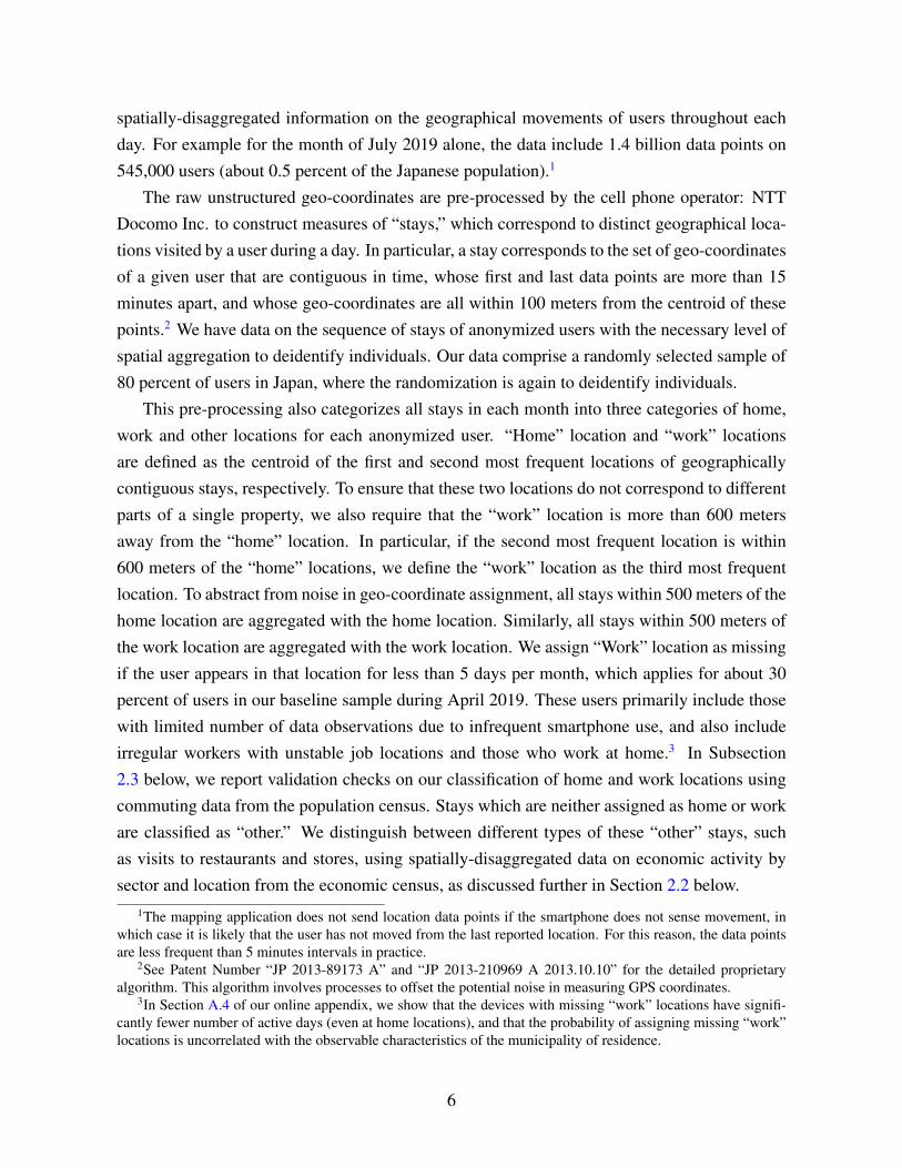
Figure 3: Distances of Commuting and Non-Commuting Trips
(A) Distribution of Distances of Work and Other Stays from Home Locations
(B) Average Distances of Different Types of Other Stays from Home Locations
(0.75) (Note: Panel (A): Distributions of distance in kilometers of work locations from home location and ofother stays from home locations during weekdays and weekends. Panel (B): Distributions of distance in kilometersfor each type of other stay from home locations during weekdays and weekends. Results for our baseline sampleof users in the Tokyo metropolitan area in April 2019.
densities of stays for “Wholesale and Retail” and “Accommodations, Eating, Drinking” occur ataround 6pm on weekdays, corroborating the fact that these activities are typically concentratedafter work during the week. Additionally, for “Accommodations, Eating, Drinking,” we find asmaller peak around noon on weekdays, capturing lunch time.
Fact 3. Non-commuting trips are closer to home. We now show that non-commuting tripsexhibit different spatial patterns from commuting trips, such that observed bilateral commutingflows provide an incomplete picture of patterns of travel within urban areas. In Panel (A) ofFigure 3, we display the distribution of distances from home locations to work locations andfrom home locations to other stays for our baseline sample of users in the Tokyo metropolitanarea in the month of April 2019. We find that other stays are concentrated closer to home than
12
work stays, with average distances travelled of 7.34 and 9.04 kilometers respectively duringweekdays, with an even larger difference in distances travelled at the weekend. In Panel (B) ofFigure 3, we display the distribution of distances travelled for each type of other stay separately.We find that “Wholesale and Retail” and “Accommodations, Eating, Drinking” stays are con-centrated closer to home than “Finance, Real Estate, Communication, and Professional” and“Other Services stays.” This clustering of other stays closer to home highlights the relevanceof these non-commuting trips for residential location decisions. More generally, these differ-ences in the geographical pattern of stays suggests that focusing on commuting trips yields anincomplete picture of bilateral patterns of travel.
Fact 4. Trip chains. We now provide evidence of trip chains, in which non-commuting tripsoccur on the way from home and work. In Figure 4, we use the fact that in the smartphone datawe observe the sequence of stays originating from a user’s home location and ending at a user’shome location (without going back home in between each stay), which we term “round trips.”Using this information, we divide all other stays that occur along such round trips into fourmutually-exclusive categories: (i) HH stays, in which the other stay is part of a round trip thatdoes not include the work location; (ii) HW stays, in which the other stay happens on the wayfrom the home location to the work location; (iii) WH stays, in which the other stay happens onthe way back from the work location to the home location; (iv) WW stays, in which the otherstay happens in between two stays at the work location (e.g. a visit to a restaurant in the middleof the working day). Panel A shows the frequency of these four different types of other staysaggregating across weekdays and weekends, while Panel B shows their frequency for weekdaysand weekends separately. We find that the majority of non-commuting trips occur separatelyfrom commuting trips (53 percent), which is driven primarily by weekends (79 percent) whenusers are significantly less likely to visit workplaces (Figure 2). Nevertheless, a substantialfraction of non-commuting trips (47 percent) occur as part of commuting trips (47 percent),highlighting the relevance of jointly modelling these two types of trips.
Taking the findings of this section as a whole, we have shown that non-commuting trips arefrequent, are closely related to consumption, exhibit different spatial patterns from commutingtrips, and can occur as part of trip chains. Each of these four features of our smartphone dataguides our theoretical modelling of commuting and non-commuting trips in the next section.
4 Theoretical Framework
In this section, we develop our quantitative urban model of internal city structure that incorpo-rates both commuting and non-commuting trips, where the derivations for all theoretical resultsin this section are reported in Section B of the online appendix.
13
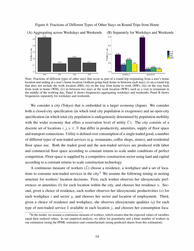
Figure 4: Fractions of Different Types of Other Stays on Round Trips from Home
(A) Aggregating across Weekdays and Weekends (B) Separately for Weekdays and Weekends
Note: Fractions of different types of other stays that occur as part of a round trip originating from a user’s homelocation and ending at a user’s home location (without going back home in between each stay); (i) on a round tripthat does not include the work location (HH); (ii) on the way from home to work (HW); (iii) on the way backfrom work to home (WH); (iv) in between two stays at the work location (WW), such as a visit to restaurant inthe middle of the working day; Panel A shows frequencies aggregating weekdays and weekends; Panel B showsfrequencies separately for weekdays and weekends.
We consider a city (Tokyo) that is embedded in a larger economy (Japan). We considerboth a closed-city specification (in which total city population is exogenous) and an open-cityspecification (in which total city population is endogenously determined by population mobilitywith the wider economy that offers a reservation level of utility U ). The city consists of adiscrete set of locations i, j, n ∈ N that differ in productivity, amenities, supply of floor spaceand transport connections. Utility is defined over consumption of a single traded good, a numberof different types of non-traded services (e.g. restaurants, coffee shops, stores), and residentialfloor space use. Both the traded good and the non-traded services are produced with laborand commercial floor space according to constant returns to scale under conditions of perfectcompetition. Floor space is supplied by a competitive construction sector using land and capitalaccording to a constant returns to scale construction technology.
A continuous measure of workers (L) choose a residence, a workplace and a set of loca-tions to consume non-traded services in the city.8 We assume the following timing or nestingstructure for workers’ location decisions. First, each worker observes her idiosyncratic pref-erences or amenities (b) for each location within the city, and chooses her residence n. Sec-ond, given a choice of residence, each worker observes her idiosyncratic productivities (a) foreach workplace i and sector g, and chooses her sector and location of employment. Third,given a choice of residence and workplace, she observes idiosyncratic qualities (q) for eachtype of non-traded service k available in each location j, and chooses her consumption loca-
8In the model, we assume a continuous measure of workers, which ensures that the expected values of variablesequal their realized values. In our empirical analysis, we allow for granularity and a finite number of workers inour estimation (using the PPML estimator) and counterfactuals (using predicted shares from this estimation).
14

tion for each type of non-traded service. Fourth, given a choice of residence, workplace, andthe set of consumption locations, she observes idiosyncratic shocks (ν) over different possi-ble travel routes: home-consume-home, work-consume-work, home-consume-work-home, orhome-work-consume-home. We choose this nesting structure because it permits a transpar-ent decomposition of residents and land prices into the contribution of travel access and theresidual of amenities, but the importance of consumption access is robust across other nestingstructures. We also compare the predictions of our model with the special case abstracting fromconsumption trips, which corresponds to a conventional urban model, in which workers chooseworkplace and residence and consume only traded goods.
4.1 Preferences
The indirect utility for worker ω who chooses residence n, works in location i and sector g ∈ K,and consumes non-traded service k ∈ KS (where KS ⊂ K) in location j(k) using route r(k)
is assumed to take the following Cobb-Douglas form:
Unig{j(k)r(k)} (ω) ={Bnbn (ω)
(P Tn
)−αTQ−α
H
n
}{ai,g (ω)wi,g} (1)
×
{ ∏k∈KS
[P Sj(k)/
(qj(k) (ω)
)]−αSk}{dni{j(k)r(k)}∏k∈KS
νr(k)(ω)
}
0 < αT , αH , αSk < 1, αT + αH +∑k∈KS
αSk = 1,
where we use the notation j(k) to indicate that that non-traded service k is consumed in asingle location j that is an implicit function of the type of non-traded service k; r(k) ∈ R ≡{HH,WW,HW,WH} indicates the “route” choice of whether to visit consumption locationsfrom home (HH), from work (WW ), on the way from home to work (HW ), or on the wayfrom work to home (WH) for each non-traded service k; KS ⊂ K is the subset of sectors thatare non-traded; the first term in brackets captures a residence component of utility; the secondterm in brackets corresponds to a workplace component; the third term in brackets reflects anon-traded services component; the fourth term in brackets reflects a travel cost component.
The first, residence component includes amenities (Bn) that are common for all workersin residence n; the idiosyncratic amenity draw for residence n for worker ω (bn(ω)); the priceof the traded good (P T
n ); and the price of residential floor space (Qn). We allow the commonamenities (Bn) to be either exogenous or endogenous to the surrounding concentration of eco-nomic activity in the presence of agglomeration forces, as discussed further below. The second,workplace component comprises the wage per efficiency unit in sector g in workplace i (wi,g)and the idiosyncratic draw for productivity or efficiency units of labor for worker ω in sector
15

g in workplace i (ai,g(ω)).9 The third, non-traded services component depends on the price ofthe non-traded service k in the location j(k) where it is supplied (P S
j(k) for k ∈ KS) and theidiosyncratic draw for quality for that service in that location (qj(k)(ω) for k ∈ KS). The fourthcomponent captures the iceberg travel cost for each combination of residence, workplace, con-sumption locations and routes (dni{j(k)r(k)}) and the idiosyncratic draw for route preference foreach non-traded sector (νr(k)(ω) for k ∈ KS).
To capture trip chains, we model the iceberg travel cost for each combination of residencen, workplace i, consumption location j(k) and route r(k) (dni{j(k)r(k)}) as follows:
dni{j(k)r(k)} = exp(−κW τWni )∏k∈KS
exp(−κSk τSnij(k)r(k)). (2)
The first term before the product sign captures the cost of commuting from residence n toworkplace i without any detour to consume non-traded services, which depends on travel time(τWni ) and the commuting cost parameter (κW ), where overall commuting travel time is the sumof that in each direction:
τWni = τni + τin. (3)
The second term in equation (2) captures the additional travel costs involved in consuming eachtype of non-traded service k in location j(k) by the route r(k), which depends on the additionaltravel time involved (τSnij(k)r(k)) and the consumption travel cost parameter (κSk ). This additionaltravel time depends on the route taken: whether the worker visits consumption location j(k)
from home (r(k) = HH), from work (WW ), on the way from home to work (HW ), or on theway from work to home (WH):
τSnij(k)HH = τnj + τjn, τSnij(k)WW = τij + τji, (4)
τSnij(k)HW = τnj + τji − τni, τSnij(k)WH = τij + τjn − τin,
where the negative terms on the second line above reflects the fact that the worker travels indi-rectly between residence n and workplace i via consumption location j on one leg of her journeybetween home and work, and hence does not incur the direct travel time between residence nand workplace i for that leg.10
We make the conventional assumption in the location choice literature following McFadden(1974) that the idiosyncratic shocks are drawn from an extreme value distribution. In particular,
9Although we model the workplace idiosyncratic draw as a productivity draw, there is a closely-related formu-lation in which it is instead modelled as an amenity draw.
10While we capture the relative importance of the consumption of non-traded services using the Cobb-Douglasexpenditure shares (αSk ), the frequency of trips can also differ across non-traded sectors, as shown in Figure 1. InSection C.1 of the online appendix, we explicitly incorporate this additional type of heterogenegity and show thatthe model is isomorphic up to a reinterpretation of the parameters κSk . Therefore, all of our counterfactual resultsare unaffected by this extension of the model except for the interpretation of the estimated κSk .
16
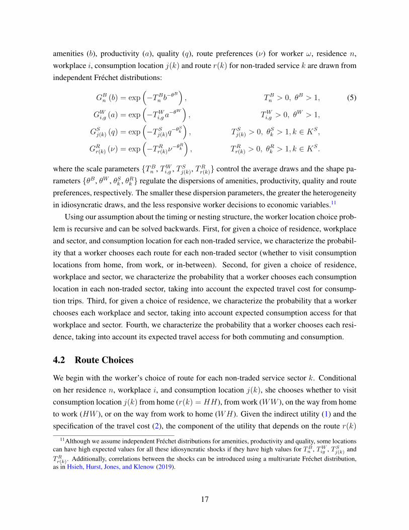
amenities (b), productivity (a), quality (q), route preferences (ν) for worker ω, residence n,workplace i, consumption location j(k) and route r(k) for non-traded service k are drawn fromindependent Frechet distributions:
GBn (b) = exp
(−TBn b−θ
B), TBn > 0, θB > 1, (5)
GWi,g (a) = exp
(−TWi,g a−θ
W), TWi,g > 0, θW > 1,
GSj(k) (q) = exp
(−T Sj(k)q
−θSk), T Sj(k) > 0, θSk > 1, k ∈ KS,
GRr(k) (ν) = exp
(−TRr(k)ν
−θRk), TRr(k) > 0, θRk > 1, k ∈ KS.
where the scale parameters {TBn , TWi,g , T Sj(k), TRr(k)} control the average draws and the shape pa-
rameters {θB, θW , θSk , θRk } regulate the dispersions of amenities, productivity, quality and routepreferences, respectively. The smaller these dispersion parameters, the greater the heterogeneityin idiosyncratic draws, and the less responsive worker decisions to economic variables.11
Using our assumption about the timing or nesting structure, the worker location choice prob-lem is recursive and can be solved backwards. First, for given a choice of residence, workplaceand sector, and consumption location for each non-traded service, we characterize the probabil-ity that a worker chooses each route for each non-traded sector (whether to visit consumptionlocations from home, from work, or in-between). Second, for given a choice of residence,workplace and sector, we characterize the probability that a worker chooses each consumptionlocation in each non-traded sector, taking into account the expected travel cost for consump-tion trips. Third, for given a choice of residence, we characterize the probability that a workerchooses each workplace and sector, taking into account expected consumption access for thatworkplace and sector. Fourth, we characterize the probability that a worker chooses each resi-dence, taking into account its expected travel access for both commuting and consumption.
4.2 Route Choices
We begin with the worker’s choice of route for each non-traded service sector k. Conditionalon her residence n, workplace i, and consumption location j(k), she chooses whether to visitconsumption location j(k) from home (r(k) = HH), from work (WW ), on the way from hometo work (HW ), or on the way from work to home (WH). Given the indirect utility (1) and thespecification of the travel cost (2), the component of the utility that depends on the route r(k)
11Although we assume independent Frechet distributions for amenities, productivity and quality, some locationscan have high expected values for all these idiosyncratic shocks if they have high values for TBn , TWig , TSj(k) andTRr(k). Additionally, correlations between the shocks can be introduced using a multivariate Frechet distribution,as in Hsieh, Hurst, Jones, and Klenow (2019).
17

for non-traded service k is given by:
δnij(k)r(k)(ω) = exp(−κSk τSnij(k)r(k))νr(k)(ω). (6)
where the first component is the route-specific travel cost and the second component is the id-iosyncratic route preference. Under our assumption of independent route draws νr(k)(ω) acrosseach non-traded sector k, each worker chooses the route r(k) that maximizes δnij(k)r(k)(ω) in-dependently for each sector k.
Using our independent extreme value assumption, the route choice probability is charac-terized by a logit form. In particular, the probability that a worker living in residence n andemployed in workplace i consuming non-traded service k in location j(k) chooses the router(k) (λRr(k)|nij(k)) is:
λRr(k)|nij(k) =TRr(k) exp(−θRk κSk τSnij(k)r(k))∑
r′∈R TRr′(k) exp(−θRk κSk τSnij(k)r′(k))
. (7)
Using the properties of the extreme value distribution, we can also compute the expectedcontribution to utility from the travel cost from consumption trips
dSnij(k) = Enij(k)
[δnij(k)r(k)(ω)
]= ϑRk
[∑r′∈R
TRr′(k) exp(−θRk κSk τSnij(k)r′(k))
] 1
θRk
(8)
where ϑRk ≡ Γ(θRk −1
θRk
)and Γ(·) is the Gamma function.
4.3 Consumption Choices
We next describe the worker’s decision of where to consume each type of non-traded service,given these expected travel costs. Conditional on living in residence n and being employed inworkplace i, each worker chooses a consumption location j(k) for each non-traded service k,after observing her idiosyncratic draws for the quality of non-traded services (d), but beforeobserving her idiosyncratic route preferences (ν). Therefore, each worker chooses the con-sumption location j(k) that maximizes the contribution to indirect utility (1) from consumingthat non-traded service k, taking into account the expected travel costs across alternative routes:
γnij(k) (ω) =[P Sj(k)/
(qj(k) (ω)
)]−αSk dSnij(k), k ∈ KS. (9)
where dSnij(k) is the expected travel cost across these alternative routes from equation (8) above.12
12Although for simplicity we assume that workers choose a single consumption location for each non-traded ser-vice, it is straightforward to extend the model to incorporate multiple consumption locations, by allowing workersto make multiple discrete choices for each non-traded service.
18
Using our extreme value assumption, the probability that a worker living in residence n andemployed in workplace i consumes non-traded service k in location j(k) (λSj(k)|ni) is:
λSj(k)|ni =T Sj(k)
(P Sj(k)
)−θSk (dSnij(k)
) θSkαSk
∑`∈N T
S`(k)
(P S`(k)
)−θSk (dSni`(k)
) θSkαSk
, k ∈ KS, (10)
which we term the conditional consumption probability, since it is computed conditional on res-idence n and workplace i. This probability depends on destination characteristics (the price ofnon-traded services P S
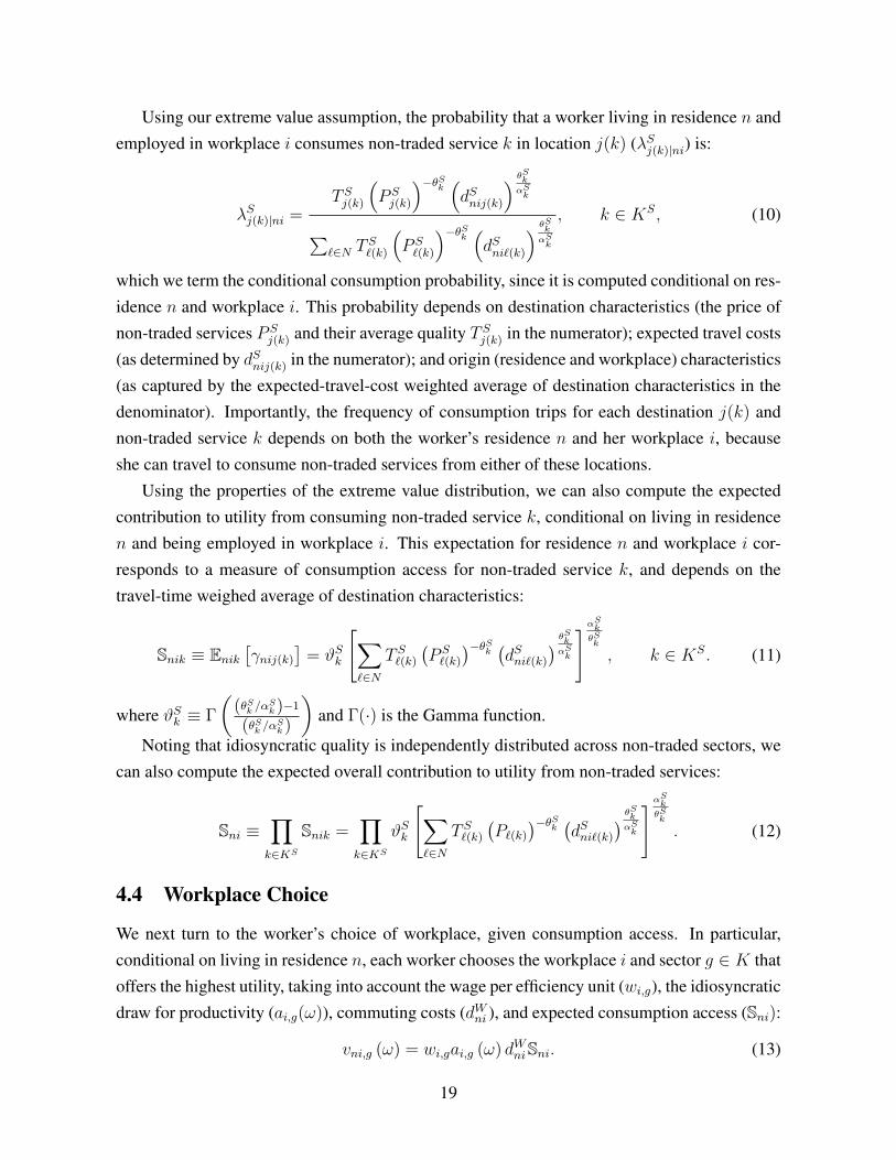
j(k) and their average quality T Sj(k) in the numerator); expected travel costs(as determined by dSnij(k) in the numerator); and origin (residence and workplace) characteristics(as captured by the expected-travel-cost weighted average of destination characteristics in thedenominator). Importantly, the frequency of consumption trips for each destination j(k) andnon-traded service k depends on both the worker’s residence n and her workplace i, becauseshe can travel to consume non-traded services from either of these locations.
Using the properties of the extreme value distribution, we can also compute the expectedcontribution to utility from consuming non-traded service k, conditional on living in residencen and being employed in workplace i. This expectation for residence n and workplace i cor-responds to a measure of consumption access for non-traded service k, and depends on thetravel-time weighed average of destination characteristics:
Snik ≡ Enik[γnij(k)
]= ϑSk
[∑`∈N
T S`(k)
(P S`(k)
)−θSk (dSni`(k)
) θSkαSk
]αSkθSk
, k ∈ KS. (11)
where ϑSk ≡ Γ
((θSk /αSk )−1
(θSk /αSk )
)and Γ(·) is the Gamma function.
Noting that idiosyncratic quality is independently distributed across non-traded sectors, wecan also compute the expected overall contribution to utility from non-traded services:
Sni ≡∏k∈KS
Snik =∏k∈KS
ϑSk
[∑`∈N
T S`(k)
(P`(k)
)−θSk (dSni`(k)
) θSkαSk
]αSkθSk
. (12)
4.4 Workplace Choice
We next turn to the worker’s choice of workplace, given consumption access. In particular,conditional on living in residence n, each worker chooses the workplace i and sector g ∈ K thatoffers the highest utility, taking into account the wage per efficiency unit (wi,g), the idiosyncraticdraw for productivity (ai,g(ω)), commuting costs (dWni ), and expected consumption access (Sni):
vni,g (ω) = wi,gai,g (ω) dWniSni. (13)
19
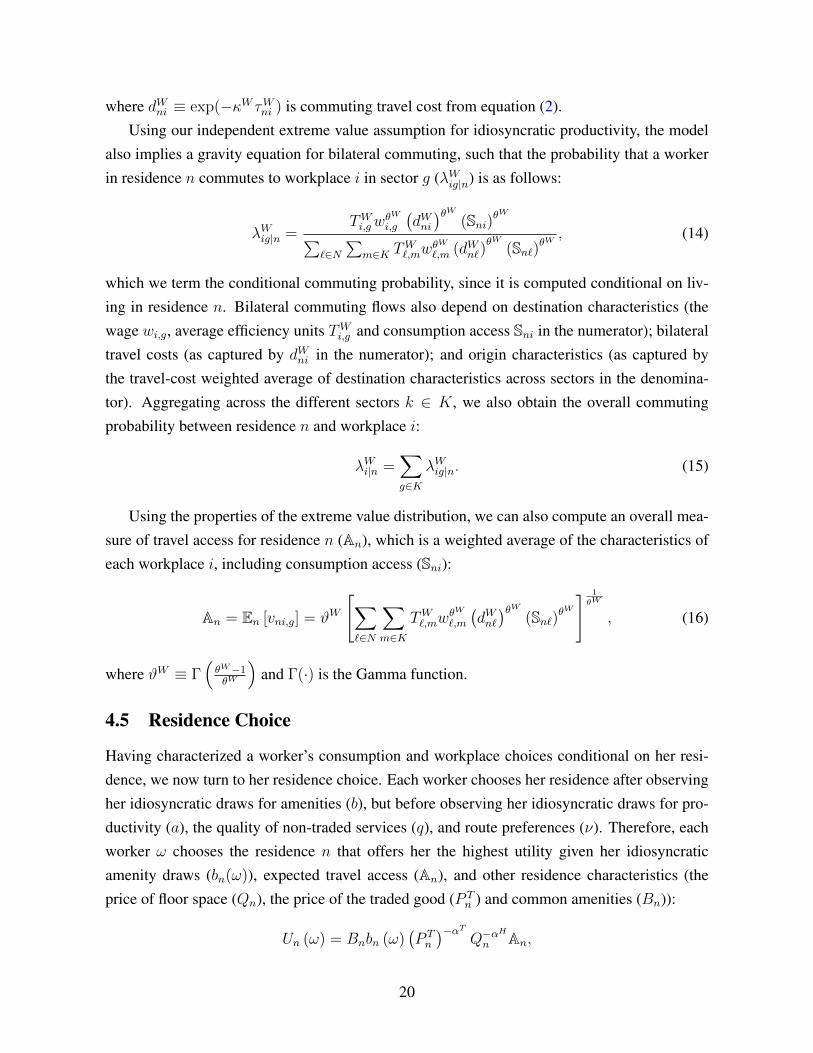
where dWni ≡ exp(−κW τWni ) is commuting travel cost from equation (2).Using our independent extreme value assumption for idiosyncratic productivity, the model
also implies a gravity equation for bilateral commuting, such that the probability that a workerin residence n commutes to workplace i in sector g (λWig|n) is as follows:
λWig|n =TWi,gw
θW
i,g
(dWni)θW
(Sni)θW∑
`∈N∑
m∈K TW`,mw
θW`,m (dWn`)
θW(Sn`)θ
W, (14)
which we term the conditional commuting probability, since it is computed conditional on liv-ing in residence n. Bilateral commuting flows also depend on destination characteristics (thewage wi,g, average efficiency units TWi,g and consumption access Sni in the numerator); bilateraltravel costs (as captured by dWni in the numerator); and origin characteristics (as captured bythe travel-cost weighted average of destination characteristics across sectors in the denomina-tor). Aggregating across the different sectors k ∈ K, we also obtain the overall commutingprobability between residence n and workplace i:
λWi|n =∑g∈K
λWig|n. (15)
Using the properties of the extreme value distribution, we can also compute an overall mea-sure of travel access for residence n (An), which is a weighted average of the characteristics ofeach workplace i, including consumption access (Sni):
An = En [vni,g] = ϑW
[∑`∈N
∑m∈K
TW`,mwθW
`,m
(dWn`)θW
(Sn`)θW
] 1
θW
, (16)
where ϑW ≡ Γ(θW−1θW
)and Γ(·) is the Gamma function.
4.5 Residence Choice
Having characterized a worker’s consumption and workplace choices conditional on her resi-dence, we now turn to her residence choice. Each worker chooses her residence after observingher idiosyncratic draws for amenities (b), but before observing her idiosyncratic draws for pro-ductivity (a), the quality of non-traded services (q), and route preferences (ν). Therefore, eachworker ω chooses the residence n that offers her the highest utility given her idiosyncraticamenity draws (bn(ω)), expected travel access (An), and other residence characteristics (theprice of floor space (Qn), the price of the traded good (P T
n ) and common amenities (Bn)):
Un (ω) = Bnbn (ω)(P Tn
)−αTQ−α
H
n An,
20
Using our extreme value assumption for idiosyncratic amenities, the probability that eachworker chooses residence n (λBn ) depends on its relative attractiveness in terms of travel access(An), and residential characteristics (Bn, PT,n and Qn):
λBn =TBn B
θB
n AθB
n
(P Tn
)−αT θBQ−α
HθB
n∑`∈N T
B` B
θB` AθB
` (P T` )−αT θB
Q−αHθB
`
. (17)
Taking expectations over idiosyncratic amenities, expected utility from living in the citydepends on the travel access and other residential characteristics of all locations within the city:
E [u] = ϑB
[∑`∈N
TB` BθB
` AθB
`
(P T`
)−αT θBQ−α
HθB
`
] 1
θB
. (18)
where ϑB ≡ Γ(θB−1θB
)and Γ(·) is the Gamma function.
In Section 5.2, we use these residential choice probabilities to decompose the observedvariation in economic activity into the contributions of travel access and a residual for amenities,without taking a stand on production technology and market structure in the traded and non-traded sectors. As a result, this quantitative analysis holds in an entire class of quantitativeurban models, with different specifications for production technology and market structure.
Expected income in residence n (En) in turn depends on the overall commuting probabilities(λWi|n) and expected income conditional on commuting from residence n to workplace i (Eni):
En =∑i∈N
λWi|nEni, (19)
where Eni depends on both wages and expected worker idiosyncratic productivity.
4.6 Production
When we undertake counterfactuals in Section 6, we do need to take a stand on a specific pro-duction technology and market structure. In particular, we assume that both the traded goodand non-traded services are produced using labor and commercial floor space according a con-stant returns to scale technology. We assume for simplicity that this production technology isCobb-Douglas and that production occurs under conditions of perfect competition.13 Togetherthese assumptions imply that profits are zero in each location with positive production:
P Ti =
1
Ai,kwβ
T
i,kQ1−βTi , 0 < βT < 1, k ∈ K/KS, (20)
P Si(k) =
1
Ai,kwβ
S
i,kQ1−βSi , 0 < βS < 1, k ∈ KS,
13In Section C.2 of the online appendix, we show that our specification is isomorphic to a model of monopolisticcompetition under free entry, once we allow for agglomeration forces (equation (25) below).
21
where Ai,k is productivity in location i in sector k.We allow productivity (Ai,k) to be either exogenous or endogenous to the surrounding con-
centration of economic activity because of agglomeration forces, as discussed further below.We assume no-arbitrage between residential and commercial floor space, and across the differ-ent sectors in which commercial floor space is used, such that there is a single price for floorspace within each location (Qi). In general, the wage per efficiency unit (wi,k) differs acrossboth sectors and locations, because workers draw efficiency units for each sector and locationpair, and hence each sector and location pair faces an upward-sloping supply function for effec-tive units of labor. Finally, we assume that the traded good is costlessly traded within the cityand wider economy and choose it as our numeraire, such that:
P Ti = 1 ∀ i ∈ N. (21)
4.7 Market Clearing
The price for non-traded service k in each location j (P Sj(k) for k ∈ KS) is determined by market
clearing, which equates revenue and expenditure for that sector k and location j:
P Sj(k)Aj,k
(Lj,kβS
)βS (Hj,k
1− βS
)1−βS
= αSk∑n∈N
Rn
∑i∈N
λSj(k)|niλWi|nEni, k ∈ KS, (22)
where expenditure on the right-hand side equals the sum across locations of workers travellingto consume non-traded service k in location j; Lj,k is the labor input adjusted for expectedidiosyncratic worker productivity in sector k in location j; Rn is the measure of residents inlocation n; and recall that λSj(k)|ni is the conditional consumption probability andEni is expectedworker income for residence n and workplace i.
Labor market clearing equates the measure of workers employed in workplace j in sector kto the measure of workers commuting from all residences n to that workplace j in sector k:
Lj,k =∑n∈N
λWjk|nRn, k ∈ K, (23)
where we use Lj,k without a tilde to denote the measure of workers without adjusting for effec-tive units of labor; and recall that λWjk|n is the conditional commuting probability.
Land market clearing equates the demand for residential floor space (Hi,U ) plus commercialfloor space in each sector (Hi,k) to the total supply of floor space (Hi):
Hi = Hi,U +∑k∈K
Hi,k. (24)
22

4.8 General Equilibrium
We begin by considering the case in which productivity (Ai,k), amenities (Bi) and the supplyof floor space (Hi) are exogenously determined. The general equilibrium of the model is ref-erenced by the price for floor space in each location (Qi), the wage in each sector and location(wi,k), the price of the non-traded good in each service sector and location (P S
i(k)), the routechoice probabilities (λRr(k)|nij(k)), the conditional consumption probabilities (λSj(k)|ni), the condi-tional commuting probabilities (λWik|n), the residence probabilities (λBn ), and the total measure ofworkers living in the city (L), where we focus on the open-city specification, in which the totalmeasure of workers is endogenously determined by population mobility with the wider econ-omy. These eight equilibrium variables are determined by the system of eight equations givenby the land market clearing condition for each location (24), the labor market clearing condi-tion for each location (23), the non-traded goods market clearing condition for each locationand service sector (22), the route choice probabilities (7), the conditional consumption proba-bilities (10), the conditional commuting probabilities (14), the residence probabilities (17), andthe population mobility condition that equates expected utility (18) to the reservation utility inthe wider economy (U ).
4.9 Agglomeration Forces and Endogenous Floor Space
We next extend the analysis to allow productivity and amenities to be endogenous to the sur-rounding concentration of economic activity through agglomeration forces and to allow for anendogenous supply of floor space. In both the traded and non-traded sector, we allow produc-tivity (Ai,k) to depend on production fundamentals and production externalities. Productionfundamentals (ai,k) capture features of physical geography that make a location more or lessproductive independently of neighboring economic activity (e.g. access to natural water). Pro-duction externalities capture productivity benefits from the density of employment across allsectors (Li/Ki), where employment density is measured per unit of geographical land area:14
Ai,k = ai,k
(LiKi
)ηW(25)
where Li =∑
k∈K Li,k is the total employment in location i, and ηW parameters the strength ofproduction externalities, which we assume to the same across all sectors.
In addition to the pecuniary externalities from consumption access, we allow residentialamenities (Bn) to depend on residential fundamentals and residential externalities. Residentialfundamentals (bn) capture features of physical geography that make a location a more or less
14We assume for simplicity that production externalities depend solely on a location’s own employment density,but we can also allow for the case in where are spillovers of these production externalities across locations.
23

attractive place to live independently of neighboring economic activity (e.g. green areas). Res-idential externalities capture the effects of the surrounding density of residents (Li/Ki) and aremodeled symmetrically to production externalities:15
Bn = bn
(Rn
Kn
)ηB(26)
where ηB parameters the strength of residential externalities.We follow the standard approach in the urban literature of assuming that floor space is
supplied by a competitive construction sector that uses land K and capital M as inputs. In par-ticular, we assume that floor space (Hi) is produced using geographical land (Ki) and buildingcapital (Mi) according to the following constant return scale technology:
Hi = Mµi K
1−µi , 0 < µ < 1. (27)
Using cost minimization and zero profits, this construction technology implies a constant elas-ticity supply function for floor space as in Saiz (2010):
Qi = ψiH1−µµ
i (28)
where ψi depends solely on geographical land area (Ki) and parameters.Given these agglomeration forces and endogenous floor space, the determination of general
equilibrium remains the same as above, except that productivity (An), amenities (Bn) and thesupply of floor space (Hn) are now endogenously determined by equations (25), (26) and (28).
5 Quantitative Analysis
In this section, we use our theoretical model to quantify the contributions of workplace accessand consumption access to location choices. The key insight underlying our approach is thatthe observed consumption and commuting probabilities in our smartphone data can be used toreveal the relative valuation placed by users on different locations as consumption and work-place locations, and hence can be used to estimate travel access in a theory-consistent way. InSection 5.1, we develop a sequential procedure to estimate the model’s parameters. In Section5.2, we use these estimated parameters and model’s residential choice probabilities to quantifythe relative importance of workplace access, consumption access and residential amenities inexplaining the observed spatial concentration of economic activity.
15As for production externalities above, we assume that residential externalities depend solely on a location’sown residents density, but we can allow spillovers of these residential externalities across locations.
24
5.1 Estimation Procedure
We begin by discussing the estimation and calibration of the model’s parameters. We proceedin a number of steps, where each step uses additional model structure. First, we calibratethe Frechet dispersion parameters for commuting, consumption, and residence choices (θW ,θSk , θB, respectively), and the shares of consumer expenditure on housing (αH), traded goods(αT ), and each type of non-traded service (αSk ) using central values from the existing empiricalliterature and the observed data. Second, we estimate the worker’s route choice problem foreach non-traded service and obtain an estimate of the expected travel cost for consumption trips(dSnij(k)). Third, we estimate her consumption choice problem conditional on her residence andworkplace, and obtain an estimate of the travel time parameter for consumption trips (φSk =
θSkκSk/α
Sk ) and consumption access (Sni). Fourth, we estimate her commuting choice problem,
and obtain an estimate of the travel time parameter for commuting trips (φW = θWκW ) andtravel access (An). Fifth, we calibrate the remaining parameters using the observed data andcentral values from the existing empirical literature.
5.1.1 Preference Parameters (θW , θB, θSk , αH , αT and αSk ) (Step 1)
In our first step, we calibrate the preference dispersion parameters (θW , θSk and θB) and expen-diture shares (αH , αT , αSk ). We set the preference dispersion parameters for commuting, con-sumption and residence choices equal to θW = θSk = θB = 6, which consistent with the rangeof estimated values for these parameters. In the existing literature on commuting, Ahlfeldt,Redding, Sturm, and Wolf (2015) estimates a preference dispersion parameter for workplace-residence choices of 6.83 using the division of Berlin by the Berlin Wall; Heblich, Redding, andSturm (2020) estimates a value for the same parameter of 5.25 using the construction of Lon-don’s 19th-century railway network; and Kreindler and Miyauchi (2019) estimates the sameparameter of 8.3 using information on the spatial dispersion of income in Dhaka, Bangladesh.In Section D.2.1 of the online appendix, we provide an over-identification check on our model’spredictions, using the property that its predictions for residential income depend importantlyon these parameter values. In particular, we compare the model’s predictions for residentialincome in each Tokyo municipality to separate data on residential income not used in its cali-bration. Although our model is necessarily an abstraction, we find a strong positive relationshipbetween the model’s predictions and the observed data.
Fewer empirical estimates are available for the preference dispersion parameter for con-sumption trips (θSk ), which determines the elasticity of consumption trips and consumption ex-penditure with respect to changes in the cost of sourcing non-traded services. Our calibratedvalue for this parameter of θSk = 6 is in line with the existing empirical literature that has esti-
25

mated elasticities of substitution across retail stores. In particular, Atkin, Faber, and Gonzalez-Navarro (2018) estimates an elasticity of substitution of 3.9 using Mexican data, while Couture,Gaubert, Handbury, and Hurst (2019) estimates an elasticity of substitution of 6.5 using USdata. In Section D.2.2 of the online appendix, we provide another overidentification check onour model’s predictions, using the property that its predictions for non-traded service prices ineach location are sensitive to this parameter value. Again we show that there is a strong positiverelationship between the model’s predictions and the observed data.
Finally, we calibrate the Cobb-Douglas expenditure share parameters using aggregate dataon observed expenditure shares in Japan. We set the share of expenditure on residential floorspace equal to αH = 0.25, which also corresponds to the values in Davis and Ortalo-Magne(2011) and Ahlfeldt, Redding, Sturm, and Wolf (2015). We set the expenditure share parameterfor each type of non-traded service (αSk ) equal to the observed expenditure share on that sectorfor the Tokyo metropolitan area. Lastly, we solve for the implied traded goods expenditureshare: αT = 1− αH −
∑k∈KS αSk .
5.1.2 Estimating the Route-Choice Probabilities (Step 2)
In our second step, we estimate expected consumption travel costs (dSnij(k)), using the model’spredictions for route choice (HH , WW , HW , WH) and our smartphone data. From the routechoice probability (7), the probability of choosing route r(k) for non-traded service k condi-tional on residence n, workplace i, and consumption location j(k) can be written as:
λRr(k)|nij(k) =exp(−φRk τSnij(k)r(k))ξ
Rr(k) exp(uRnij(k)r(k))
ζRnij(k)
, (29)
where uRnij(k)r(k) is a stochastic error that captures idiosyncratic determinants of route choice,given residence, workplace, and consumption location.
We estimate this route choice probability using the Poisson Pseudo Maximum Likelihood(PPML) estimator of Santos Silva and Tenreyro (2006).16 The estimated semi-elasticity of traveltime (φRk ) in equation (29) is a composite of the response of consumption trips to travel costs(θRk ) and the response of travel costs to travel times (κSk ), such that φRk = θRk κ
Sk . The estimated
route fixed effect ξRr(k) corresponds to the tendency that each route is chosen conditional on traveltime, such that ξRr(k) = TRr(k). The estimated residence-workplace-consumption-location fixedeffect ζRnij(k) captures the average tendency that routes are chosen for each residence, workplace,consumption location, such that ζRnij(k) =
∑`∈R T
R`(k) exp(−θRk κSk τSnij(k)`(k)).
Table 2 presents the estimation results for each of the different types of non-traded services:“Finance, Real Estate, Communication, and Professional”; “Wholesale and Retail”; “Accom-
16We find a similar pattern of results if we estimate this choice probability using the multinomial logit model.
26
modation, Eating and Drinking”; “Medical, Welfare and Health Care”; “Other Services”. In thefirst row, we report the coefficient on the travel time (φRk ). In the second to fourth row report,we report the coefficient on the dummy variables for each route choice, where r(k) = HH isthe excluded category. Two features of Table 2 are noteworthy. First, we estimate a negativeand statistically significant composite coefficient on travel time (−φRk = −θRk κSk ), highlightingits relevance for route choice. Second, we estimate negative and statistically significant coef-ficients on the indicator variables for the included route choices (r(k) ∈ {HW,WH,WW})relative to the excluded category of r(k) = HH . These results imply a high average preferencefor consuming non-traded services from home, consistent with Figure 4 in Section 3.
Using these estimates of φRk and ξRr(k), we construct adjusted expected travel costs for con-sumption trips conditional on residence n and workplace i from equation (8) above as:
dSnij(k) ≡(dSnij(k)
)1/κSk = ϑRk
[∑r′∈R
ξRr′(k) exp(−φRk τSnij(k)r′(k))
] 1
φRk
, (30)
where ϑRk is again ϑRk ≡ Γ(θRk −1
θRk
)and recall R = {HH,HW,WH,WW}.
In this second step of our estimation, the composite semi-elasticity of travel time (φRk =
θRk κSk/α
Sk ) is a sufficient statistic for the impact of travel time on route choices, as estimated
from the route choice probabilities (29). We do not need to separate out the contributions ofθRk and κSk to the overall value of this parameter. Similarly, our adjusted measure of expected
travel costs (dSnij(k) ≡(dSnij(k)
)1/κSk) from equation (30) is a sufficient statistic for the impact of
expected travel costs on workers choice of consumption locations, workplace and residence inthe subsequent steps of our estimation below. We do not need to separate out the contributionsof 1/κSk and dSnij(k) to the overall value of adjusted expected travel costs (dSnij(k)).
5.1.3 Estimating Consumption Access (Sni) (Step 3)
In our third step, we estimate the consumption choice probability and consumption access (Sni),using the observed frequencies of consumption trips to reveal the relative attractiveness of eachlocation for each type of non-traded service. From the conditional consumption probabilities(10), the probability that a worker travels to consume non-traded service k in location j(k),conditional on residence n and workplace i is:
λSj(k)|ni =ξSj(k)
(dSnij(k)
)−φSkexp
(uSnij(k)
)ζSni,k
, (31)
where dSnij(k) is our estimated adjusted expected travel costs from equation (30); and uSnij(k) is astochastic error that captures idiosyncratic determinants of consumption travel costs.
27
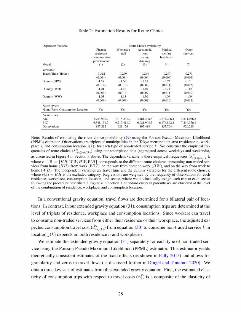
Table 2: Estimation Results for Route Choice
Dependent Variable: Route Choice ProbabilityFinance
realestatecommunication
professional
Wholesaleretail
Accomoda-tionseating
drinking
Medicalwelfare
healthcare
Otherservices
Model: (1) (2) (3) (4) (5)
VariablesTravel Time (Hours) -0.312 -0.269 -0.264 -0.297 -0.271
(0.004) (0.004) (0.004) (0.004) (0.004)Dummy (HW) -1.58 -1.66 -1.75 -1.67 -1.61
(0.010) (0.010) (0.009) (0.011) (0.012)Dummy (WH) -1.04 -1.16 -1.10 -1.23 -1.12
(0.009) (0.010) (0.009) (0.011) (0.010)Dummy (WW) -1.03 -1.13 -1.30 -1.09 -1.09
(0.009) (0.009) (0.008) (0.010) (0.011)
Fixed-effectsHome-Work-Consumption Location Yes Yes Yes Yes Yes
Fit statisticsAIC 3,753,940.7 7,015,231.9 3,461,408.3 3,674,206.4 4,511,086.5BIC 6,348,159.7 9,717,411.9 6,081,904.7 6,174,892.1 7,210,376.1Observations 887,212 921,176 895,488 857,704 920,268
Note: Results of estimating the route choice probability (29) using the Poisson Pseudo Maximum Likelihood(PPML) estimator. Observations are triplets of municipalities in the Tokyo metropolitan area (residence n, work-place i, and consumption location j(k)) for each type of non-traded service k. We construct the empirical fre-quencies of route choice (λRr(k)|nij(k)) using our smartphone data (aggregated across weekdays and weekends),as discussed in Figure 4 in Section 3 above. The dependent variable is these empirical frequencies (λRr(k)|nij(k)),where r ∈ R ≡ {HH,WW,HW,WH} corresponds to the different route choices: consuming non-traded ser-vices from home (HH), from work (WW ), on the way from home to work (HW ), and on the way from work tohome (WH). The independent variables are travel time and the dummy variables for the different route choices,where r(k) = HH is the excluded category. Regressions are weighted by the frequency of observations for eachresidence, workplace, consumption-location, and sector, where we stochastically assign each trip to each sectorfollowing the procedure described in Figure 4 in Section 3. Standard errors in parentheses are clustered at the levelof the combination of residence, workplace, and consumption location.
In a conventional gravity equation, travel flows are determined for a bilateral pair of loca-tions. In contrast, in our extended gravity equation (31), consumption trips are determined at thelevel of triplets of residence, workplace and consumption locations. Since workers can travelto consume non-traded services from either their residence or their workplace, the adjusted ex-pected consumption travel cost (dSnij(k)) from equation (30) to consume non-traded service k inlocation j(k) depends on both residence n and workplace i.
We estimate this extended gravity equation (31) separately for each type of non-traded ser-vice using the Poisson Pseudo Maximum Likelihood (PPML) estimator. This estimator yieldstheoretically-consistent estimates of the fixed effects (as shown in Fally 2015) and allows forgranularity and zeros in travel flows (as discussed further in Dingel and Tintelnot 2020). Weobtain three key sets of estimates from this extended gravity equation. First, the estimated elas-ticity of consumption trips with respect to travel costs (φSk ) is a composite of the elasticity of
28

consumption trips with respect to travel costs (θSk /αSk ) and the elasticity of travel costs with
respect to travel times (κSk ) in equation (10), such that φSk = θSkκSk/α
Sk . Second, the estimated
consumption destination fixed effect (ξSj(k)) in equation (31) captures the average attractivenessof consumption destination j(k) for service k in terms of its price for that non-traded service(P S
j(k)) and quality draws (T Sj(k)) in equation (10), such that:
ξSj(k) = T Sj(k)
(P Sj(k)
)−θSk . (32)
Third, the estimated residence fixed effect in equation (31) corresponds to the denominator inthe conditional consumption probability in equation (10) and captures the overall attractivenessof residence n in terms of its access to all consumption locations `(k) for service k:
ζSni,k =∑`∈N
T S`(k)
(P S`(k)
)−θSk (dSni`(k)
)−φSk. (33)
From these estimated fixed effects, we recover a theoretically-consistent estimate of con-sumption access for each type of non-traded service (Snik). Indeed, consumption access can berecovered from either the consumption destination fixed effects or the residence fixed effects.First, summing the estimated consumption destination fixed effects (ξSj(k)) weighted by the es-
timated bilateral travel cost ((dSni`(k)
)−φSk) across locations, and using our calibrated values of
θSk and αSk , we obtain our baseline estimate of consumption access:
Sni =∏k∈KS
Γ
(θSk /α
Sk − 1
θSk /αSk
)[∑`∈N
ξS`(k)
(dSni`(k)
)−φSk]αSkθSk. (34)
Second, using the estimated residence fixed effects (ζSni,k), and our calibrated values of θSk
and αSk , we obtain another estimate of consumption access: Sni =∏
k∈KS
[Γ(θSk /α
Sk−1
θSk /αSk
)] (ζSni,k
)αSkθSk .
As sample size becomes sufficiently large, these two sets of estimates of consumption accessconverge asymptotically towards one another if the model is a correct specification of the truedata generating process, as shown in an international trade context in Fally (2015). In practice,even in our finite sample, we find that these two estimates are extremely highly correlated withone another, as shown in Section D.4 of the online appendix.
In Table 3, we report the results of estimating the consumption extended gravity equation(31) for each type of non-traded service separately. In all cases, we estimate negative andstatistically significant semi-elasticities of consumption trips with respect to travel costs (−φSk ).We find that these estimated semi-elasticities are relatively constant across the different typesof consumption trips, ranging from -1.08 to -1.19, with the most localized consumption tripsobserved for “Finance, Real Estate, Communication, and Professional” and “Medical, Welfare
29

and Health Care”. In Section D.3 of the online appendix, we report a specification check inwhich model the relationship between consumption trips and travel costs non-parametricallyand demonstrate a similar pattern of results.17
Table 3: Estimation Results for Consumption Location Choice
Dependent Variable: Consumption Location Choice ProbabilityFinance
realestatecommunication
professional
Wholesaleretail
Accomodationseating
drinking
Medicalwelfare
healthcare
Otherservices
Model: (1) (2) (3) (4) (5)
Variableslog dSnij(k) -1.15 -1.12 -1.09 -1.19 -1.08
(0.040) (0.036) (0.035) (0.038) (0.036)
Fixed-effectsHome and Work Location Pairs Yes Yes Yes Yes YesConsumption Location Yes Yes Yes Yes Yes
Fit statisticsAIC 129,480.5 130,876.3 131,837.4 128,831.5 132,020.7BIC 291,657.6 293,164.9 294,084.1 290,841.4 294,295.3Observations 2,981,924 2,983,860 2,983,134 2,979,020 2,983,618
Note: Results of estimating the consumption trip probability (31) using the Poisson Pseudo Maximum Likelihood(PPML) estimator. Observations are triplets of municipalities in the Tokyo metropolitan area (residence n, work-place i, and consumption location j(k)). Each column regresses the consumption trip probability for each typeof non-traded service on the adjusted expected travel cost (dSnij(k)) from the previous step, consumption locationfixed effects, and residence-workplace pair fixed effects. Standard errors in parentheses are clustered two-way onconsumption location and residence-workplace pair.
5.1.4 Estimating the Workplace Choice and Travel Access (An) (Step 4)
In our fourth step, we estimate the workplace choice probability and overall travel access (An),by using the observed frequencies of commuting trips to reveal the relative attractiveness ofresidences and workplaces. From our parameterization of commuting costs and equations (14)and (15), the probability that a worker commutes from residence n to workplace i can be writtenas the following extended gravity equation:
λWi|n =ξWi exp
(−φW τWni
)(Sni)θ
W
exp(uWni)
ζWn, (35)
where uWni is a stochastic error that reflects idiosyncratic determinants of bilateral commutingcosts not captured in bilateral travel times (τni).
17As a specification check, we re-estimated the consumption gravity equation under the false assumption thatall consumption trips originate from home. As shown in Table D.5.1 in Section D.5 of the online appendix,we find substantially smaller semi-elasticities in this robustness check (ranging from -0.8 to -0.6), highlighting theimportance of endogenous route choice. Furthermore, we find a better model fit incorporating route choice than thisalternative specification, as evident from the smaller Akaike Information Criteria (AIC) or Bayesian InformationCriteria (BIC) than in Panel (B) of Table D.5.1.
30

In a conventional gravity equation for commuting, the key bilateral determinant of commut-ing flows is bilateral travel time τWni . In contrast, in our extended gravity equation for commuting(35), a worker’s choice of workplace depends on the extent to which it enhances the worker’saccess to consumption opportunities, which in turn depends on the worker’s residence. There-fore, consumption access (Sni) varies bilaterally with both workplace and residence, and entersas an additional determinant of bilateral commuting flows alongside bilateral travel time
We estimate this extended commuting gravity equation (35) using the Poisson Pseudo Max-imum Likelihood (PPML) estimator, our measures of commuting travel times (τWni ), and ourestimates of bilateral consumption access (Sni) from the previous step. We again obtain threekey sets of estimates from this extended gravity equation. First, the estimated semi-elasticityof commuting flows with respect to travel times (φW ) in equation (35) is again a compositeof the response of commuting flows to commuting costs (θW ) and the response of commutingcosts to travel times (κW ) in equation (14), such that φW = θWκW . Second, the estimatedworkplace fixed effect (ξWi ) in equation (35) captures the average attractiveness of workplace iacross sectors in terms of its wage (wi,g) and productivity draws (TWi,g ):
ξWi =∑m∈K
TWi,mwθW
i,m. (36)
Third, the estimated residence fixed effect (ζWn ) in equation (35) corresponds to the denominatorin the conditional commuting probability in equation (14) and captures the overall attractivenessof residence n in terms of its travel-time weighted access to all workplaces:
ζWn =∑`∈N
∑m∈K
TW`,mwθW
`,m exp(−φW τWn`
)(Sn`)θ
W
. (37)
From these estimated fixed effects, we recover a theoretically-consistent measure of overalltravel access. Indeed, as for consumption access in the previous step, we can recover travel ac-cess in two different ways. First, summing the estimated workplace fixed effects (ζWi ) weightedusing the estimated bilateral travel costs (exp
(−φW τWni
)) across locations, and using θW , we
obtain our baseline estimate of travel access:
An = Γ
(θW − 1
θW
)[∑`∈N
ξW` exp(−φW τWn`
)(Sn`)θ
W
] 1
θW
. (38)
Second, using the estimated residence fixed effects (ζWn ) and θW , we obtain another estimate ofworkplace access: An = Γ
(θW−1θW
) (ζWn) 1
θW . As sample size becomes sufficiently large, thesetwo sets of estimates of travel access again converge asymptotically towards one another if themodel is a correct specification of the true data generating process. In practice, even in our finitesample, we find that these two estimates are extremely highly correlated with one another, asshown in Section D.4 of the online appendix.
31
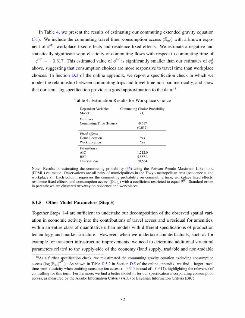
In Table 4, we present the results of estimating our commuting extended gravity equation(31). We include the commuting travel time, consumption access (Sn`) with a known expo-nent of θW , workplace fixed effects and residence fixed effects. We estimate a negative andstatistically significant semi-elasticity of commuting flows with respect to commuting time of−φW = −0.617. This estimated value of φW is significantly smaller than our estimates of φSkabove, suggesting that consumption choices are more responsive to travel time than workplacechoices. In Section D.3 of the online appendix, we report a specification check in which wemodel the relationship between commuting trips and travel time non-parametrically, and showthat our semi-log specification provides a good approximation to the data.18
Table 4: Estimation Results for Workplace Choice
Dependent Variable: Commuting Choice ProbabilityModel: (1)
VariablesCommuting Time (Hours) -0.617
(0.037)
Fixed-effectsHome Location YesWork Location Yes
Fit statisticsAIC 1,212.0BIC 5,557.3Observations 58,564
Note: Results of estimating the commuting probability (35) using the Poisson Pseudo Maximum Likelihood(PPML) estimator. Observations are all pairs of municipalities in the Tokyo metropolitan area (residence n andworkplace i). Each column regresses the commuting probability on commuting time, workplace fixed effects,residence fixed effects, and consumption access ((Sn`)) with a coefficient restricted to equal θW . Standard errorsin parentheses are clustered two-way on residence and workplaces.
5.1.5 Other Model Parameters (Step 5)
Together Steps 1-4 are sufficient to undertake our decomposition of the observed spatial vari-ation in economic activity into the contributions of travel access and a residual for amenities,within an entire class of quantitative urban models with different specifications of productiontechnology and market structure. However, when we undertake counterfactuals, such as forexample for transport infrastructure improvements, we need to determine additional structuralparameters related to the supply-side of the economy (land supply, tradable and non-tradable
18As a further specification check, we re-estimated the commuting gravity equation excluding consumptionaccess (log (Sn`)θ
W
). As shown in Table D.5.2 in Section D.5 of the online appendix, we find a larger traveltime semi-elasticity when omitting consumption access (−0.649 instead of −0.617), highlighting the relevance ofcontrolling for this term. Furthermore, we find a better model fit for our specification incorporating consumptionaccess, as measured by the Akaike Information Criteria (AIC) or Bayesian Information Criteria (BIC).
32

production, and production and amenity spillovers). In our fifth step, we calibrate these param-eters directly from the data or using central values from the existing empirical literature.
We calibrate the Cobb-Douglas cost shares for labor in each sector (βS, βT ) as 0.8, whichare broadly consistent with the labor share on production costs for Tokyo metropolitan area. Weassume a standard share of land in construction costs of µ = 0.75. We explore a range of valuesfor the production and residential agglomeration parameters ranging from zero to the valuesestimated in Ahlfeldt, Redding, Sturm, and Wolf (2015): ηW ∈ [0, 0.08] and ηB ∈ [0, 0.15],which spans most of the existing empirical estimates in the meta-analyses of Melo, Graham,and Noland (2009) and Ahlfeldt and Pietrostefani (2019).
5.2 Quantifying the Role of Workplace and Consumption Access
We now use our estimates from Steps 1-4 above to quantify the contributions of travel accessand the residual of residential amenities to explaining the observed spatial concentration ofeconomic activity and to examine the relative importance of workplace access and consumptionaccess for overall travel access. Re-writing the residential choice probabilities (17), we have:(
λBn)1/θB
QαH
n = BnAn. (39)
The left-hand side of this relationship corresponds to a summary measure of the relativeattractiveness of locations. A larger share of residents (λBn ) and/or a higher price of floor space(Qn) both imply that a location is a more attractive place to live. On the right-hand side, Bn is acomposite amenities parameter that includes common amenities (Bn), the parameter determin-ing average idiosyncratic amenities (TBn ), the common price of the traded good (P T
n = P T = 1),and the common reservation level of utility (U ):
Bn ≡ Bn
(TBn)1/θB (
P Tn
)−αT (U/ϑB
)−1(40)
In these residential choice probabilities (39), we observe the share of residents (λBn ) and theprice of floor space (Qn), and we estimated travel access (An) in equation (38). Therefore, wecan use these residential choice probabilities (39) to recover the unobserved composite ameni-ties (Bn) as a structural residual that exactly rationalizes the observed data as an equilibriumof the model. This residential choice decomposition has an intuitive interpretation. If a loca-tion has a high share of residents (λBn ) and high price of floor space (Qn) on the left-hand side,despite having relatively low values of composite access (An) on the right-hand side, this isrationalized in the model by that location having relatively high residential amenities (Bn).
We now decompose the variance of our summary measure of the relative attractiveness oflocations into the contributions of travel access (An) and residential amenities (Bn). In partic-ular, we use a regression-based variance decomposition from the international trade literature.
33
We estimate an ordinary least squares (OLS) regression of each of the components on the right-hand side of the residential choice probabilities (39) on our summary measure of the relativeattractiveness of locations from the left-hand side:
lnAn = cA0 + cA1 ln((λBn)1/θB
QαH
n
)+ uAnt, (41)
lnBn = cB0 + cB1 ln((λBn)1/θB
QαH
n
)+ uBnt,
Noting that OLS is a linear estimator with mean zero residuals, and using the residentialchoice probabilities (39), we have cA0 + cB0 = 0 and cA1 + cB1 = 1. Implicitly, this variancedecomposition allocates the covariance terms equally across each of the two components. Therelative values of the slope coefficients {cB1 , cA1 } provide measures of the relative importanceof travel access (An) and residential amenities (Bn) in explaining the observed variation in oursummary measure of the relative attractiveness of locations.
We next examine the relative importance of workplace access and consumption access foroverall travel access, by considering a special case of our quantitative urban model withoutconsumption trips (αSk = 0 for all k ∈ KS , αT = 1 − αH , λSj(k)|ni = 0 and Sni = 1). Inthis special case, we ignore the data on consumption trips, and estimate a standard quantitativeurban model of workplace-residence choice using only the data on commuting trips. As a result,travel accessibility (Anocons
n ) depends on workplace access alone, and can be constructed usingthe estimates from our extended gravity equation estimation of equation (35), but omitting theconsumption access term (log (Sn`)θ
W
):
Anoconsn = Γ
(θW − 1
θW
)[∑`∈N
ξW` exp(−φW τWn`
)] 1
θW
, (42)
where φW and ξW` are the estimated travel time coefficient and workplace fixed effects from theextended commuting gravity equation (35). Using this measure of travel access without con-sumption trips (Anocons
n ) in equation (39), we can recover a measure of amenities without con-sumption trips (Bnocons
n ), and implement our variance decomposition in equation (41) above.19
Table 5 reports the results of these variance decompositions for our model including con-sumption trips (Panel A) and the special case excluding consumption trips (Panel B). Obser-vations correspond to municipalities in the Tokyo metropolitan area for which we have landprice data. We measure the price of floor space (Qn) using the observed land price data (Qn)
19As a robustness check, Panel (B) of online appendix Table D.5.3 construct travel access without consumptiontrips (Anocons
n ) using the estimates of φW and ξW` from a conventional commuting gravity equation excludingconsumption access. Although the estimated travel time coefficients differ between these two gravity equationspecifications, we find a similar pattern of results for the relative importance of consumption access and residentialamenities in this robustness test as in our baseline specification.
34

Table 5: Decomposition of our Summary Statistic for Relative Attractiveness(log
[(λBn)1/θB
QαH
n
]) into Travel Access (An) and Residential Amenities (Bn)
logAn logBn(1) (2)
Panel A: Baseline Model
logQαH
n
(λBn)1/θB 0.566 0.434
(0.049) (0.049)
Observations 201 201R2 0.403 0.284
Panel B: No Consumption Trips
logQαH
n
(λBn)1/θB 0.373 0.627
(0.036) (0.036)
Observations 201 201R2 0.352 0.606
Note: Ordinary least squares (OLS) estimates of the regression-based variance decomposition in equation (41).Panel (A) corresponds to our baseline model, in which we compute travel access (An) incorporating consumptiontrips; Panel (B) corresponds to the special case of our model in which we abstract from consumption trips (Anocons
n ),such that αSk = 0 for all k ∈ KS , αT = 1− αH , λSj(k)|ni = 0 and Sni = 1. Observations are municipalities in theTokyo metropolitan area. Heteroskedasticity robust standard errors in parentheses.
and our assumption of competitive construction sector (such that Qn ∝ Q1−µn ). In our model
including consumption trips, we find that travel access (An) is about as important as the resid-ual of residential amenities (Bn) in explaining variation in the relative attractiveness of locations(QαH
n
(λBn)1/θB ), with a contribution of 56 percent compared to 44 percent. In contrast, when we
consider a conventional quantitative urban model excluding consumption trips, we find a sub-stantially reduced contribution from travel access (Anocons
n ) of only 37 percent, with the residualof residential amenities making up the remaining 63 percent. These results suggest that a sub-stantial component of the variation in conventional measures of residential amenities that do notcontrol for consumption trips may reflect unobserved differences in consumption access. Theyalso suggest that workplace access (Anocons
n ) is far from perfectly correlated with overall travelaccess incorporating consumption trips (An), because we find a much smaller contribution fromtravel access when we restrict attention to commuting information alone.
6 Counterfactuals
We next use our theoretical framework to undertake counterfactuals for changes in travel costs toprovide further evidence on the role of consumption access in understanding the spatial concen-tration of economic activity. In particular, we examine the role of consumption trips in shaping
35
the welfare effects of transport infrastructure improvements. We undertake a counterfactual forthe construction of a new subway (underground) line in the city of Sendai and compare themodel’s predictions to the observed impact in the data.20
Before the opening of its new subway (underground) line, the city of Sendai had only oneNanboku (North-South) subway line, which had been in operation since 1987. In December2015, the new Tozai (East-West) subway line opened, thereby providing a substantial expan-sion in the overall subway network. In Section 6.1, we report reduced-form evidence on theimpact of the Tozai Subway line on floor space prices, residential population and travel access.We compare the results of differences-in-differences specifications estimated using the actualdata and the counterfactual predictions of our model. In Section 6.2, we present the model’scounterfactual predictions for the welfare gains from the opening of the Tozai Subway Line andevaluate the contribution from consumption access towards these welfare gains.
To undertake the counterfactual simulation, we solve the system of equations for a generalequilibrium of the model using an exact-hat algebra approach, in which we rewrite the counter-factual equilibrium conditions of the model in terms of the initial travel shares and endogenousvariables of the model and the counterfactual changes in these endogenous variables, as shownin Section E of the online appendix. In our baseline specification, we use the fitted valuesfor the initial travel shares from our gravity equation estimation to address potential concernsabout granularity. In Section G.5 of the online appendix, we report a robustness test using theobserved initial travel shares, and demonstrate similar results using both approaches. In ourbaseline specification, we consider the closed-city specification of the model, in which totalpopulation for the city as a whole (L) is exogenous, and hence the change in travel costs affectsworker welfare.21
6.1 Difference-in-Difference Effects of Tozai Subway Line
We start by analyzing in the impact of the Tozai Subway Line in our observed smartphone andland price data. Our analysis is based on the following difference-in-difference regression:
∆ log Yn = c0 + c1Tn + un, (43)
where n indexes Oaza; Tn is a dummy variable that equals one if the Oaza includes the newstations of the Tozai Subway Line (except for Sendai station which is also a station for the ex-isting Nanboku Subway Line) and zero otherwise; ∆ log Yn is the log difference of an outcome
20In Section F of the online appendix, we provide further evidence on the relative importance of consumptionand workplace access for location decisions by comparing the results of separate counterfactuals for changes intravel costs for commuting and consumption trips for the Tokyo metropolitan area.
21It is straightforward to instead consider the open-city specification, in which case total population is endoge-nous, and the welfare effects of the change in travel costs accrue only to landlords, as in the public finance literaturefollowing George (1879).
36
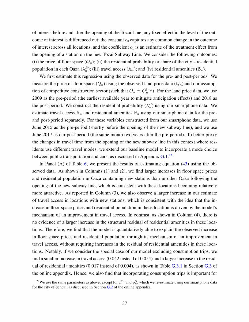
of interest before and after the opening of the Tozai Line; any fixed effect in the level of the out-come of interest is differenced out; the constant c0 captures any common change in the outcomeof interest across all locations; and the coefficient c1 is an estimate of the treatment effect fromthe opening of a station on the new Tozai Subway Line. We consider the following outcomes:(i) the price of floor space (Qn); (ii) the residential probability or share of the city’s residentialpopulation in each Oaza (λBn ); (iii) travel access (An); and (iv) residential amenities (Bn).
We first estimate this regression using the observed data for the pre- and post-periods. Wemeasure the price of floor space (Qn) using the observed land price data (Qn) and our assump-tion of competitive construction sector (such that Qn ∝ Q1−µ
n ). For the land price data, we use2009 as the pre-period (the earliest available year to mitigate anticipation effects) and 2018 asthe post-period. We construct the residential probability (λBn ) using our smartphone data. Weestimate travel access An and residential amenities Bn using our smartphone data for the pre-and post-period separately. For these variables constructed from our smartphone data, we useJune 2015 as the pre-period (shortly before the opening of the new subway line), and we useJune 2017 as our post-period (the same month two years after the pre-period). To better proxythe changes in travel time from the opening of the new subway line in this context where res-idents use different travel modes, we extend our baseline model to incorporate a mode choicebetween public transportation and cars, as discussed in Appendix G.1.22
In Panel (A) of Table 6, we present the results of estimating equation (43) using the ob-served data. As shown in Columns (1) and (2), we find larger increases in floor space pricesand residential population in Oaza containing new stations than in other Oaza following theopening of the new subway line, which is consistent with these locations becoming relativelymore attractive. As reported in Column (3), we also observe a larger increase in our estimateof travel access in locations with new stations, which is consistent with the idea that the in-crease in floor space prices and residential population in these location is driven by the model’smechanism of an improvement in travel access. In contrast, as shown in Column (4), there isno evidence of a larger increase in the structural residual of residential amenities in these loca-tions. Therefore, we find that the model is quantitatively able to explain the observed increasein floor space prices and residential population through its mechanism of an improvement intravel access, without requiring increases in the residual of residential amenities in these loca-tions. Notably, if we consider the special case of our model excluding consumption trips, wefind a smaller increase in travel access (0.042 instead of 0.054) and a larger increase in the resid-ual of residential amenities (0.017 instead of 0.004), as shown in Table G.3.1 in Section G.3 ofthe online appendix. Hence, we also find that incorporating consumption trips is important for
22We use the same parameters as above, except for φW and φSk , which we re-estimate using our smartphone datafor the city of Sendai, as discussed in Section G.2 of the online appendix.
37
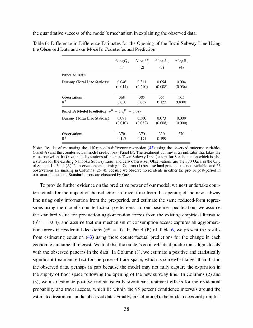
the quantitative success of the model’s mechanism in explaining the observed data.
Table 6: Difference-in-Difference Estimates for the Opening of the Tozai Subway Line Usingthe Observed Data and our Model’s Counterfactual Predictions
∆ logQn ∆ log λBn ∆ logAn ∆ logBn(1) (2) (3) (4)
Panel A: Data
Dummy (Tozai Line Stations) 0.046 0.311 0.054 0.004(0.014) (0.210) (0.008) (0.036)
Observations 368 305 305 305R2 0.030 0.007 0.123 0.0001
Panel B: Model Prediction (ηB = 0; ηW = 0.08)
Dummy (Tozai Line Stations) 0.091 0.300 0.073 0.000(0.010) (0.032) (0.008) (0.000)
Observations 370 370 370 370R2 0.197 0.191 0.199
Note: Results of estimating the difference-in-difference regression (43) using the observed outcome variables(Panel A) and the counterfactual model predictions (Panel B). The treatment dummy is an indicator that takes thevalue one when the Oaza includes stations of the new Tozai Subway Line (except for Sendai station which is alsoa station for the existing Nanboku Subway Line) and zero otherwise. Observations are the 370 Oaza in the Cityof Sendai. In Panel (A), 2 observations are missing in Column (1) because land price data is not available, and 65observations are missing in Columns (2)-(4), because we observe no residents in either the pre- or post-period inour smartphone data. Standard errors are clustered by Oaza.
To provide further evidence on the predictive power of our model, we next undertake coun-terfactuals for the impact of the reduction in travel time from the opening of the new subwayline using only information from the pre-period, and estimate the same reduced-form regres-sions using the model’s counterfactual predictions. In our baseline specification, we assumethe standard value for production agglomeration forces from the existing empirical literature(ηW = 0.08), and assume that our mechanism of consumption access captures all agglomera-tion forces in residential decisions (ηB = 0). In Panel (B) of Table 6, we present the resultsfrom estimating equation (43) using these counterfactual predictions for the change in eacheconomic outcome of interest. We find that the model’s counterfactual predictions align closelywith the observed patterns in the data. In Column (1), we estimate a positive and statisticallysignificant treatment effect for the price of floor space, which is somewhat larger than that inthe observed data, perhaps in part because the model may not fully capture the expansion inthe supply of floor space following the opening of the new subway line. In Columns (2) and(3), we also estimate positive and statistically significant treatment effects for the residentialprobability and travel access, which lie within the 95 percent confidence intervals around theestimated treatments in the observed data. Finally, in Column (4), the model necessarily implies
38
zero treatment effect for residential amenities in the absence of residential agglomeration forces(ηB = 0), which is consistent with our finding above using the observed data that the estimatedtreatment effect for residential amenities is close to zero and statistically insignificant.23
As an additional specification check, we estimate the same reduced-form regressions, butuse a dummy variable that takes the value one for Oazas that contain stations on the exist-ing Nanboku (North-South) Subway Line (which opened in 1987) rather than stations on thenew Tozai (East-West) Subway Line (which opened in 2015). If there are positive or negativenetwork effects from the new Tozai Subway Line on locations with stations on the existingNanboku Subway Line, we would expect to again detect statistically significant treatment ef-fects. In Section G.4 of the online appendix, we show that we find no evidence of statisticallysignificant treatments effects on the price of floor space, residential population, travel access,and residential amenities for this existing Nanboku Subway Line. These results are consistentwith a limited net impact of network effects on the existing subway line and suggest that ourearlier estimates for the Tozai Subway Line are indeed capturing effects specific to this newsubway line. Consistent with these findings using the observed data, we also find no evidenceof statistically significant treatment effects for the existing Nanboku Subway Line using ourcounterfactual predictions of the model.
6.2 Welfare Gains from the Tozai Subway Line
We now use our baseline closed-city version of the model to evaluate the welfare impact ofthe opening of this new subway line. In Table 7, we present the results for the different modelspecifications shown in the left-most column. In the second column, we report the percent-age point increase in expected utility for the residents of the city of Sendai. In our baselinespecification in the first row, we again assume the standard value for production agglomerationforces from the existing empirical literature (ηW = 0.08), and assume that our mechanism ofconsumption access captures all agglomeration forces in residential decisions (ηB = 0). In therobustness checks in the subsequent rows, we report results for a number of alternative specifi-cations. In the third column, we report the change in expected utility in each of these alternativespecifications as a percentage of that in our baseline specification in the first row.
As reported in Row (1), we find an increase in the flow of expected utility from the openingof the new Tozai Subway Line of 2.74 percentage points in our baseline specification. Therefore,even though we take into account the existence of other modes of transport prior to the opening
23In a robustness test in Section G.3 of the online appendix, we estimate ηB using the identifying assumptionthat the log change in residential fundamentals (bn in equation (26)) is uncorrelated with proximity to new subwaystations. We find a small estimate of ηB = 0.01. In the special case of the model that abstracts from consumptiontrips, we obtain a somewhat larger estimate of ηB = 0.05, again highlighting the importance of incorporatingconsumption trips for the model’s mechanism of travel access to explain the observed data.
39

of the new line (such as buses), we find substantial welfare gains from the reduction in bilateraltravel times achieved by the opening of the new subway line. To provide a point of comparison,Row (2) reports results for the special case of our model excluding consumption trips (αSk = 0
for all k ∈ KS , αT = 1 − αH , λSj(k)|ni = 0 and Snt = 1). In this specification, we finda welfare gain from the new subway line of 1.44 percentage points, or 53 percent of that inour baseline specification. Therefore, we find that the undercounting of travel journeys fromfocusing solely on commuting trips is quantitatively important for the evaluation of the welfareeffects of observed transport infrastructure improvements.
In Row (3), we consider another special case of the model, in which we falsely assume thatall consumption trips originate from home locations, thereby ruling out travel to consume non-traded services from work or on the way between home and work.24 In this special case, we findsomewhat larger welfare gains from the new subway line of 2.99 percentage points, or 9 percentlarger than our baseline specification. This pattern of results is intuitive, because excludingconsumption travel from work or on the way between home and work increases average traveldistances for consumption trips, and hence increases the magnitude of the welfare gain from thereduction in travel times achieved by the opening of the new subway line.
Table 7: Counterfactual Increase in Expected Utility in Sendai from the new Tozai Subway LinePercentage Point Increase in Residential Utility Relative to Baseline (%)
(1) Baseline (ηB = 0; ηW = 0.08) 2.74 1.00(2) No consumption trips 1.44 0.53(3) No trip chains for consumption trips 2.99 1.09(4) Include residential spillover (ηB = 0.15) 3.24 1.18(5) Eliminate production spillover (ηW = 0) 2.61 0.95
Note: The second column reports model counterfactuals for the percentage point increase in expected utility as a result of the reduction in traveltime from the opening of the new Tozai (East-West) subway line in the city of Sendai. The first row presents results for our baseline specification(residential agglomeration forces of ηB = 0, workplace agglomeration forces of ηW = 0.08) and the subsequent rows present results fora number of alternative specifications. The third column reports the change in expected utility in each of these alternative specifications as apercentage of the change in our baseline specification in the first row.
In the remaining two rows, we examine the sensitivity of our results to alternative assump-tions about the strength of residential and production agglomeration forces. In Row (4), weintroduce residential agglomeration forces by assuming ηB = 0.15 instead of ηB = 0. In thisspecification, we find welfare gains from the new subway line that are around 18 percent largerthan those in our baseline specification. In Row (5), we exclude productivity spillovers by as-suming ηW = 0 instead of ηW = 0.08. In this case, we find welfare gains from the new subwayline that are around 5 percent smaller than those in our baseline specification. Therefore, wefind that agglomeration forces magnify the welfare gains from transport infrastructure improve-ments, consistent with the findings of existing studies, such as Tsivanidis (2018) and Heblich,
24More specifically, we consider the limiting case in which TRr(k) → 0 for r (k) ∈ {WW,HW,WH} andTRHH > 0, which ensures that workers always travel to consume non-traded services from home.
40
Redding, and Sturm (2020). Nevertheless, the impact of these agglomeration forces on thewelfare gains from transport infrastructure improvements (comparing Rows (4) and (5) to Row(1)) is smaller than the impact of excluding consumption trips (comparing Row (2) to Row (1)),again highlighting the relevance of consumption access for the evaluation of the welfare effectsof transport infrastructure improvements.
7 Conclusions
We provide new theory and evidence on the role of consumption access in understanding thespatial concentration of economic activity. We use smartphone data that records the global po-sitioning system (GPS) location of users every 5 minutes to provide high-resolution evidenceon patterns of travel by hour and day within the Tokyo metropolitan area. Guided by our em-pirical findings, we develop a quantitative model of internal city structure that captures the factthat much of the travel that occurs within urban areas is related not to commuting but ratherto the consumption of non-traded services, such as trips to restaurants, coffee shops and bars,shopping expeditions, excursions to cinemas, theaters, music venues and museums, and visitsto professional service providers.
We begin by establishing four key empirical properties of these non-commuting trips. First,we show that they are more frequent than commuting trips, so that concentrating solely oncommuting substantially underestimates travel within urban areas. Second, we find that they areconcentrated closer to home and are more responsive to travel time than commuting trips, whichimplies that focusing solely on commuting yields a misleading picture of bilateral patterns oftravel within cities. Third, combining our smartphone data with highly spatially-disaggregateddata on employment by sector, we show that these non-commuting trips are closely related tothe availability of nontraded sectors, consistent with our modelling of them as travel to consumenon-traded services. Fourth, we find evidence of trip chains, in which these consumption tripscan occur along the journey between home and work, highlighting the relevance of jointlymodelling both commuting and consumption trips.
We next develop our quantitative theoretical model of internal city structure that incorpo-rates these consumption trips. Workers choose their preferred residence, workplace and con-sumption locations, taking into account the bilateral costs of travel and idiosyncratic draws foramenities for each residence, productivity for each workplace, service quality for each con-sumption location, and preferences for each route. We show that the observed travel dataand model’s gravity equations for commuting and consumption trips can be used to estimatetheoretically-consistent measures of travel access. We use the model’s residential choice prob-abilities to derive a summary measure of the relative attractiveness of locations based on the
41

observed share of residents and the price of floor space. We show that travel access is moreimportant than the residual of residential amenities in explaining variation in this summarymeasure of relative attractiveness, with a contribution of 56 percent compared to 44 percent. Ina special case of our model excluding consumption trips, we find a substantially smaller con-tribution from travel access of 37 percent, suggesting that conventional measures of amenitiesmay in part capture consumption access, and highlighting the usefulness of smartphone data inmeasuring consumption trips that are otherwise hard to observe.
Finally, we show how the model can be used to undertake counterfactuals for changes intransport infrastructure. We compare the model’s counterfactual predictions for the openingof a new subway line in the city of Sendai to the observed impact in the data. We show thatour model incorporating consumption access generates a similar pattern of estimated treatmenteffects as in the observed data. We show that focusing solely on commuting trips leads toan underestimate of the welfare gains from the transport improvement by around one half,because of the substantial undercounting of trips that results from abstracting from the manyother reasons besides commuting why individuals travel within urban areas.
Taken together, our findings suggest that access to consumption opportunities as well as ac-cess to employment opportunities plays a central role in understanding the spatial concentrationof economic activity.
42
ReferencesAGARWAL, S., J. B. JENSEN, AND F. MONTE (2020): “Consumer Mobility and the Local Structure of Con-
sumption Industries,” NBER Working Paper, 23616.AHLFELDT, G., AND E. PIETROSTEFANI (2019): “The Economic Effects of Density: A Synthesis,” Journal
of Urban Economics, 111, 97–107.AHLFELDT, G., S. REDDING, D. STURM, AND N. WOLF (2015): “The Economics of Density: Evidence
from the Berlin Wall,” Econometrica, 83(6), 2127–2189.ALLEN, T., C. ARKOLAKIS, AND X. LI (2017): “Optimal City Structure,” Yale University, mimeograph.ALLEN, T., S. FUCHS, S. GANAPATI, A. GRAZIANO, R. MADERA, AND J. MONTORIOL-GARRIGA (2020):
“Is Tourism Good for Locals? Evidence from Barcelona,” Dartmouth College, mimeograph.ALMAGRO, M., AND T. DOMINGUEZ-IINO (2019): “Location Sorting and Endogenous Amenities: Evidence
from Amsterdam,” NYU, mimeograph.ANAS, A., AND Y. LIU (2007): “A Regional Economy, Land Use, And Transportation Model (RELU-TRAN):
Formulation, Algorithm Design, and Testing,” Journal of Regional Science, 47(3), 415–455.ATHEY, S., B. FERGUSON, M. GENTZKOW, AND T. SCHMIDT (2018): “Experienced Segregation,” Stanford
University, mimeograph.ATKIN, D., K. CHEN, AND A. POPOV (2021): “The Returns to Face-to-Face Interactions: Knowledge
Spillovers in Silicon Valley,” MIT, mimeograph.ATKIN, D., B. FABER, AND M. GONZALEZ-NAVARRO (2018): “Retail globalization and household welfare:
Evidence from mexico,” Journal of Political Economy, 126(1), 1–73.BALBONI, C. (2019): “In Harm’s Way: Infrastructure Investments and the Persistence of Coastial Cities,”
MIT, mimeograph.BAUM-SNOW, N. (2007): “Did Highways Cause Suburbanization?,” Quarterly Journal of Economics, 122(2),
775–780.BRODA, C., AND D. E. WEINSTEIN (2006): “Globalization and the Gains from Variety,” The Quarterly journal
of economics, 121(2), 541–585.BUCHEL, K., M. V. EHRLICH, D. PUGA, AND E. VILADECANS (2020): “Calling from the Outside: The Role
of Networks in Residential Mobility,” Journal of Urban Economics, 119(103277).COUTURE, V. (2016): “Valuing the Consumption Benefits of Urban Density,” Vancouver School of Economics,
mimeograph.COUTURE, V., J. DINGEL, A. GREEN, AND J. HANDBURY (2019): “Quantifying Social Interactions Using
Smartphone Data,” Chicago Booth School of Business, mimeograph.COUTURE, V., C. GAUBERT, J. HANDBURY, AND E. HURST (2019): “Income Growth and the Distributional
Effects of Urban Spatial Sorting,” University of California, Berkeley, mimeograph.DAVIS, D. R., J. I. DINGEL, J. MONRAS, AND E. MORALES (2019): “How Segregated Is Urban Consump-
tion?,” Journal of Political Economy, 127(4), 1684–1738.DAVIS, M. A., AND F. ORTALO-MAGNE (2011): “Housing Expenditures, Wages, Rents,” Review of Economic
Dynamics, 14(2), 248–261.DIAMOND, R. (2016): “The Determinants and Welfare Implications of US Workers’ Diverging Location
Choices by Skill: 1980-2000,” 106(3), 479–524.DINGEL, J., AND F. TINTELNOT (2020): “Spatial Economics for Granular Settings,” NBER working Paper,
27287.DOLFEN, P., L. EINAV, P. J. KLENOW, B. KLOPACK, J. D. LEVIN, L. LEVIN, AND W. BEST (2019):
“Assessing the Gains from E-Commerce,” NBER Working Paper, 25610.DONALDSON, D. (2018): “Railroads of the Raj: Estimating the Impact of Transportation Infrastructure,”
American Economic Review, 108(4-5), 899–934.
43
DONALDSON, D., AND R. HORNBECK (2016): “Railroads and American Economic Growth: A Market AccessApproach,” Quarterly Journal of Economics, 131(2), 799–858.
DURANTON, G., AND M. A. TURNER (2012): “Urban Growth and Transportation,” Review of EconomicStudies, 79(4), 1407–1440.
FABER, B. (2014): “Integration and the Periphery: The Unintended Effects of New Highways in a DevelopingCountry,” Review of Economic Studies, 81(3), 1046–1070.
FALLY, T. (2015): “Structural Gravity and Fixed Effects,” Journal of International Economics, 97(1), 76–85.GEORGE, H. (1879): Progress and Poverty. Doubleday, Page & Company, New York.GLAESER, E. L., J. KOLKO, AND A. SAIZ (2001): “Consumer City,” Journal of Economic Geography, 1(1),
27–50.GORBACK, C. (2020): “Ridesharing and the Redistribution of Economic Activity,” National Bureau of Eco-
nomic Research, mimeograph.GUPTA, A., C. KONTOKOSTA, AND S. VAN NIEUWERBURGH (2020): “Take the Q Train: Value Capture of
Public Infrastructure Projects,” NBER Working Paper, 26789.HEBLICH, S., S. REDDING, AND D. STURM (2020): “The Making of the Modern Metropolis: Evidence from
London,” Quarterly Journal of Economics, 135(4), 2059–2133.HOELZLEIN, M. (2020): “Two-sided Sorting and Spatial Inequality in Cities,” Berkeley, mimeograph.HSIEH, C., E. HURST, C. I. JONES, AND P. J. KLENOW (2019): “The Allocation of Talent and U.S. Economic
Growth,” Econometrica, 87(5), 1439–1474.KREINDLER, G., AND Y. MIYAUCHI (2019): “Measuring Commuting and Economic Activity inside Cities
with Cell Phone Records,” Boston University, mimeograph.LEONARDI, M., AND E. MORETTI (2019): “Agglomeration of Urban Amenities: Evidence from Milano
Restaurants,” .MCFADDEN, D. (1974): “The Measurement of Urban Travel Demand,” Journal of Public Economics, 3(4),
303–328.MELO, P. C., D. J. GRAHAM, AND R. B. NOLAND (2009): “A Meta-analysis of Estimates of Urban Agglom-
eration Economies,” Regional Science and Urban Economics, 39(3), 332–342.MICHAELS, G. (2008): “The Effect of Trade on the Demand for Skill: Evidence from the Interstate Highway
System,” Review of Economics and Statistics, 90(4), 683–701.MONTE, F., S. REDDING, AND E. ROSSI-HANSBERG (2018): “Commuting, Migration and Local Employ-
ment Elasticities,” American Economic Review, 108(12), 3855–3890.SAIZ, A. (2010): “The Geographic Determinants of Housing Supply,” Quarterly Journal of Economics, 125(3),
1253–1296.SAMUELS, P., N. HAUSMAN, M. COHEN, AND R. SASSON (2016): “Urban Pull: The Roles of Amenities and
Employment,” Harvard University, mimeograph.SANTOS SILVA, J., AND S. TENREYRO (2006): “The Log of Gravity,” Review of Economics and Statistics,
88(4), 641–658.SEVEREN, C. (2019): “Commuting, Labor, and Housing Market Effects of Mass Transportation: Welfare and
Identification,” Federal Reserve Bank of Philadelphia.STOREYGARD, A. (2016): “Farther on Down the Road: Transport costs, Trade and Urban Growth,” Review of
Economic Studies, 83(3), 1263–1295.TSIVANIDIS, N. (2018): “The Aggregate And Distributional Effects Of Urban Transit Infrastructure: Evidence
From Bogota’s TransMilenio,” University of California, Berkeley, mimeograph.ZARATE, R. D. (2020): “Spatial Misallocation, Informality, and Transit Improvements: Evidence from Mexico
City,” University of California, Berkeley.
44