consumer theory, markets and economic welfare. topics 1. competitive consumer: preferences, budget...
TRANSCRIPT

Consumer Theory, Markets and Economic Welfare

Topics
1. Competitive consumer: preferences, budget sets, choices. Price and income effects.
2. Firms: transform multiple inputs into outputs.
3. Private ownership economy with initial ownership of goods and firms, markets, trades, prices, feasible allocation, compet. equilibrium.
4. Pareto efficiency.
5. Externalities: fundamental or not.
6. Two Fundamental Welfare Theorems, their limited relevance; other advantages of markets
Competitive Consumer (a model)
• Price-taking, rational optimizer• Acts as if it cannot affect prices (no market
power); pays for what it gets (no stealing).• Buys best affordable bundle of goods.• Best according to preferences represented
by indifference sets.• Affordable bundles = bundles in budget set.
Competitive Consumer (a model)
• Bundles• Indifference Curves, abbreviated INDIFF• Budget Sets show affordable bundles• Optimal Choices
(5, 15)
(15, 5)
(4,20)
5 15 20
(20,15)
Y
X
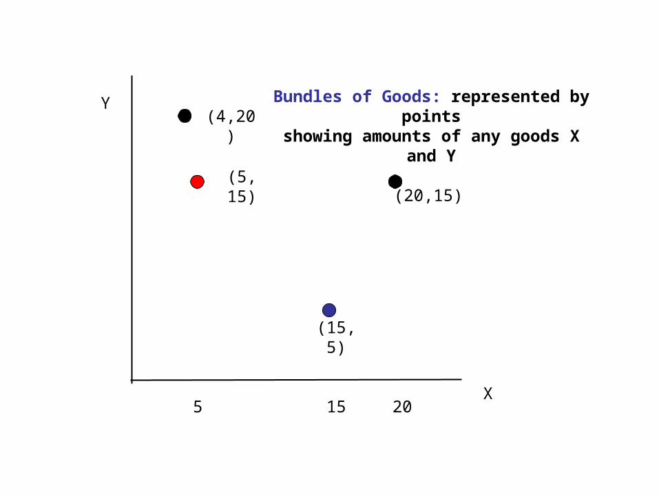
Bundles of Goods: represented by pointsshowing amounts of any goods X and Y
(5, 15)
(15, 5)
(4,20)
5 15 20
(20,15)
Y
X
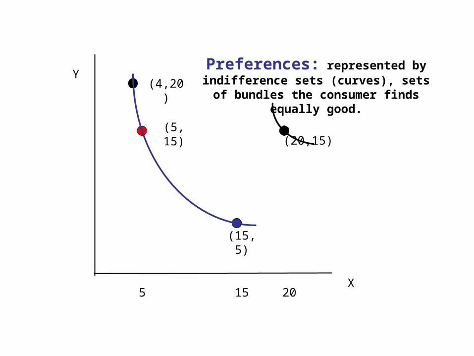
Preferences: represented by indifference sets (curves), sets of
bundles the consumer finds equally good.
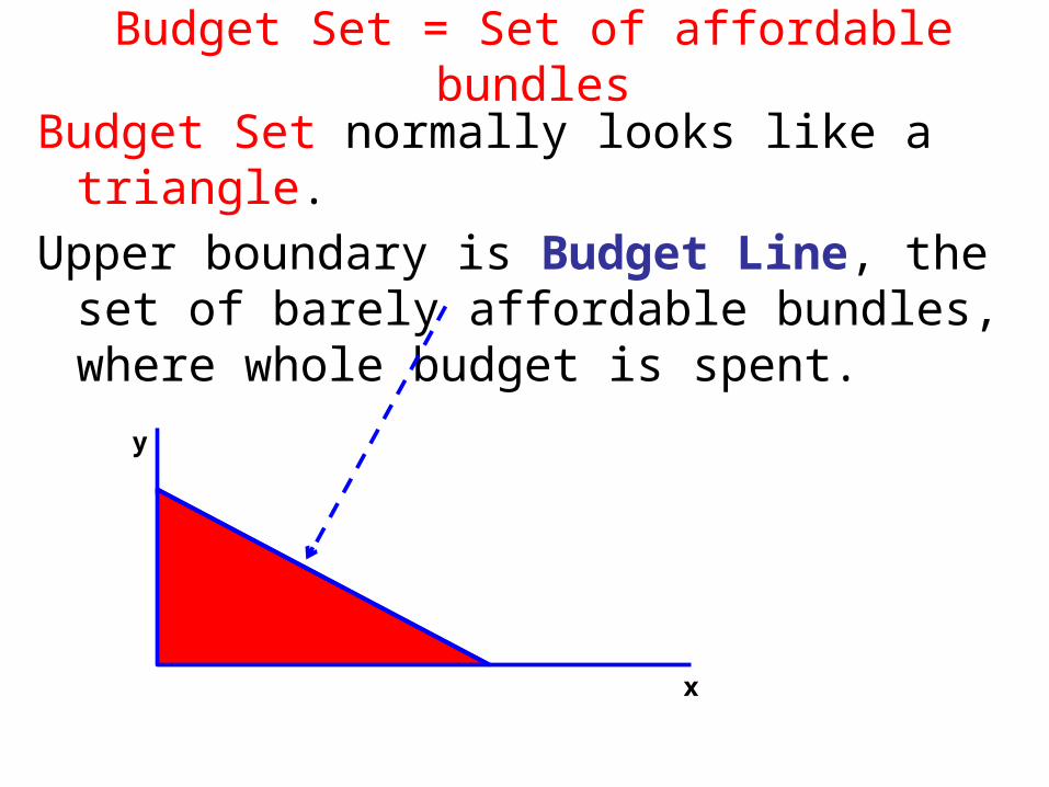
Budget Set = Set of affordable bundles
Budget Set normally looks like a triangle.
Upper boundary is Budget Line, the set of barely affordable bundles, where whole budget is spent.
y
x
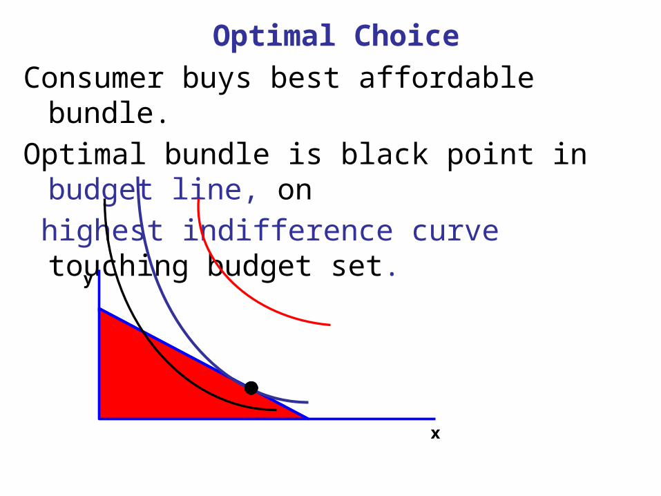
Optimal Choice
Consumer buys best affordable bundle.
Optimal bundle is black point in budget line, on
highest indifference curve touching budget set.
y
x
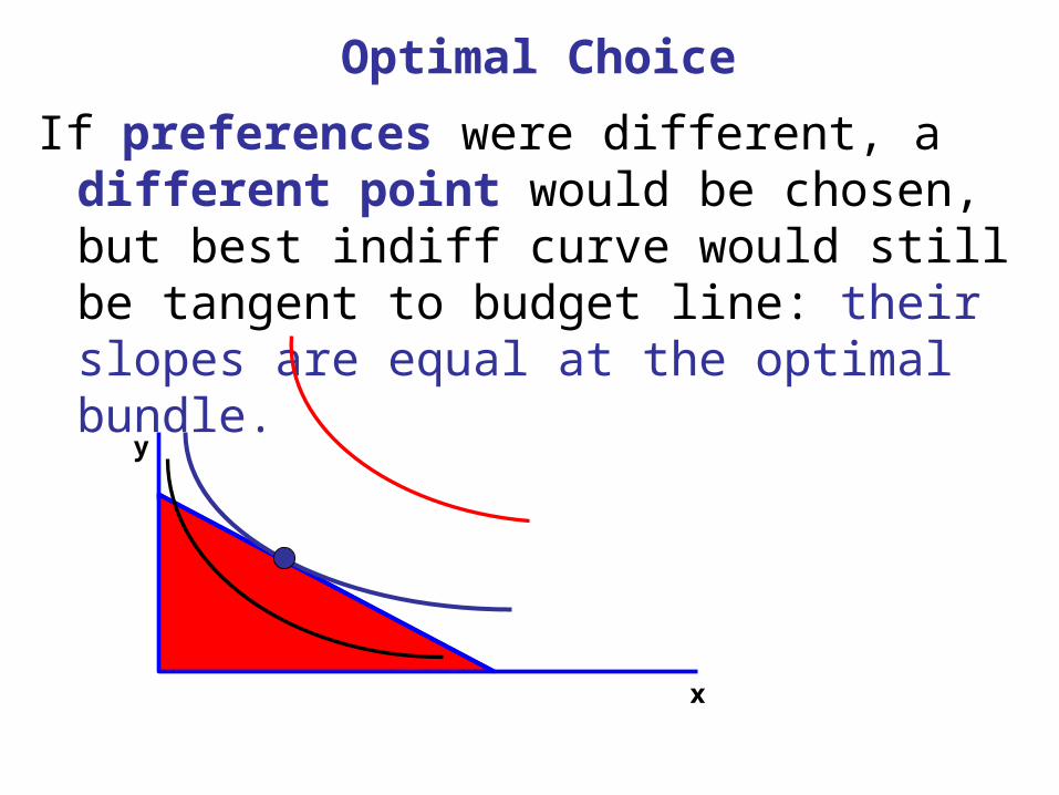
Optimal Choice
If preferences were different, a different point would be chosen, but best indiff curve would still be tangent to budget line: their slopes are equal at the optimal bundle.
y
x
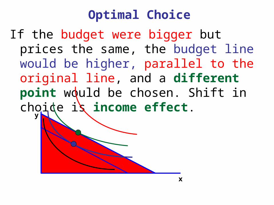
Optimal Choice
If the budget were bigger but prices the same, the budget line would be higher, parallel to the original line, and a different point would be chosen. Shift in choice is income effect.
y
x

Meaning of Indiff Curve Shapes
Negative slope of indiff curve corresponds to both goods being desired.
Curve shaped like corresponds to preference for moderate amounts of all goods, not a
large amount of one of them.y
x
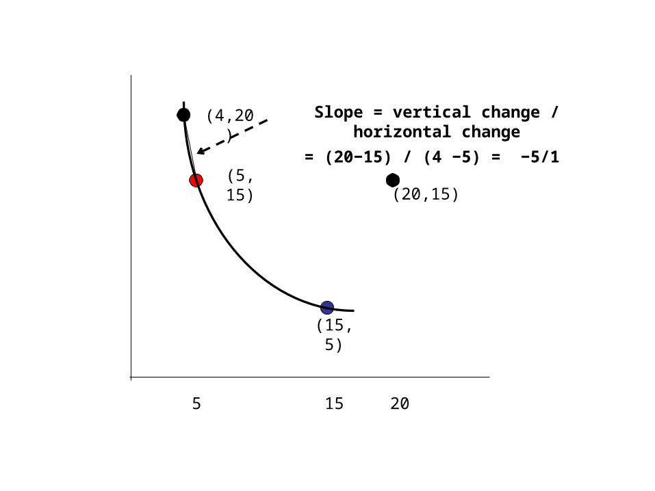
(5, 15)
(15, 5)
(4,20)
5 15 20
(20,15)
Slope = vertical change / horizontal change
= (20−15) / (4 −5) = −5/1
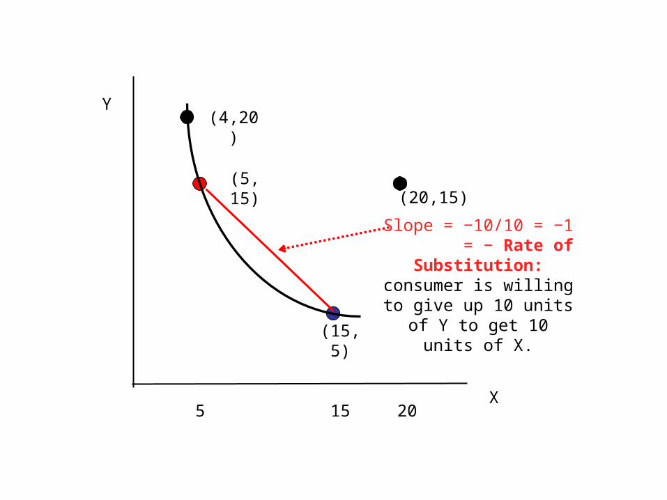
(5, 15)
(15, 5)
(4,20)
5 15 20
(20,15)
Slope = −10/10 = −1 = − Rate of Substitution: consumer is willing to give up 10 units of Y to get 10
units of X.
Y
X
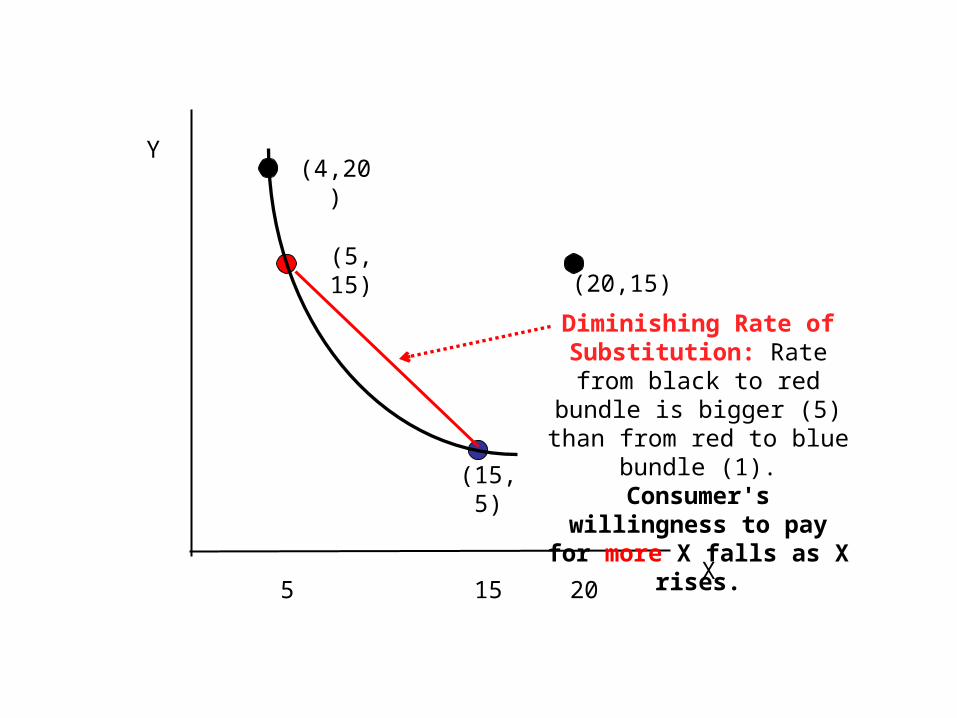
(5, 15)
(15, 5)
(4,20)
5 15 20
(20,15)
Diminishing Rate of Substitution: Rate from
black to red bundle is bigger (5) than from red to blue bundle (1). Consumer's willingness to pay for
more X falls as X rises.
Y
X
(5, 15)
(15, 5)
(4,20)
5 15 20
(20,15)
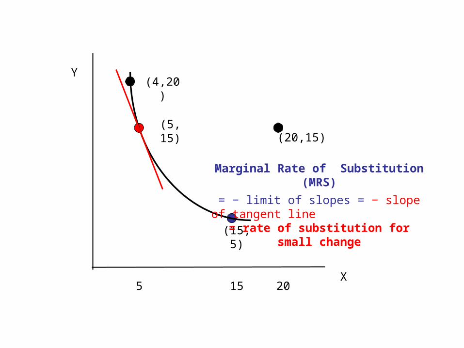
Marginal Rate of Substitution (MRS)
= − limit of slopes = − slope of tangent line = rate of substitution for small
change
Y
X

(5, 15)
(15, 5)
(4,20)
5 15 20
(20,15)
Curve shape implies preference for moderation:
average consumption (10, 10) is preferred to red and blue
bundles.
Y
X
(10, 10)
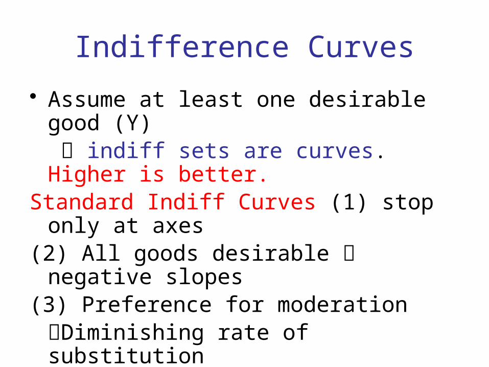
Indifference Curves
• Assume at least one desirable good (Y) indiff sets are curves. Higher is better.
Standard Indiff Curves (1) stop only at axes(2) All goods desirable negative slopes(3) Preference for moderationDiminishing rate of substitutionLess willing to pay for additional unitsIndiff curves shaped like:
(5, 15)
(15, 5)
(4,20)
5 15 20
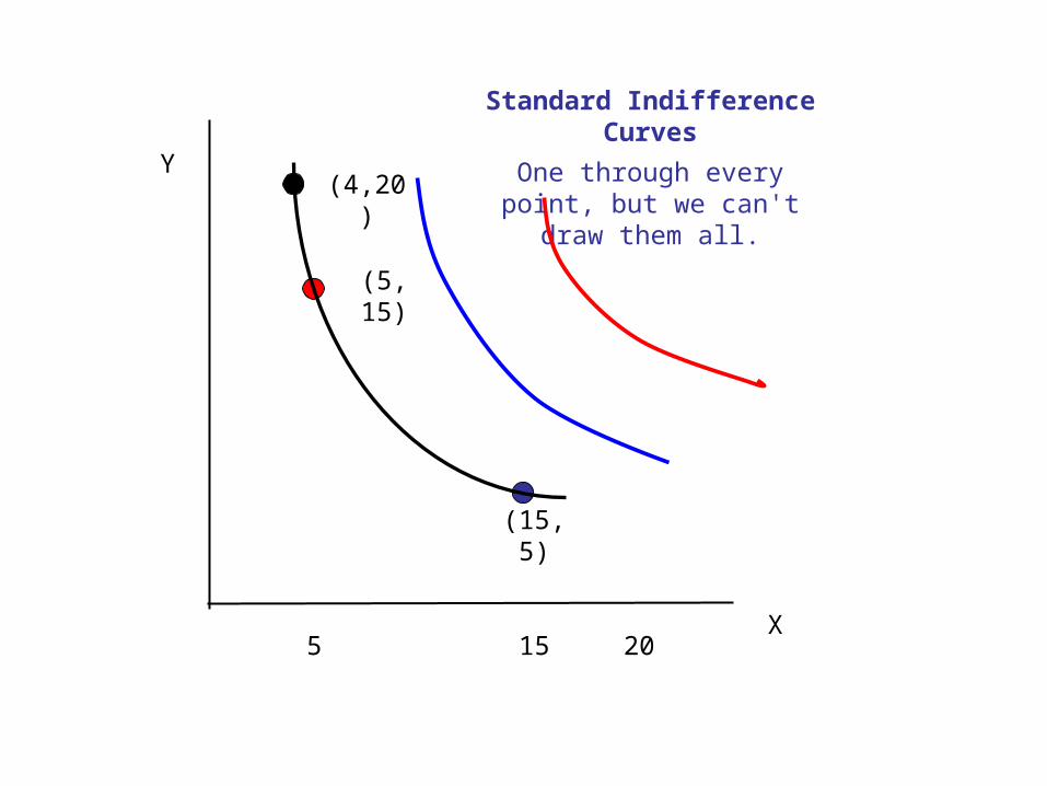
Standard Indifference Curves
One through every point, but we can't draw them all.Y
X
5 15 20
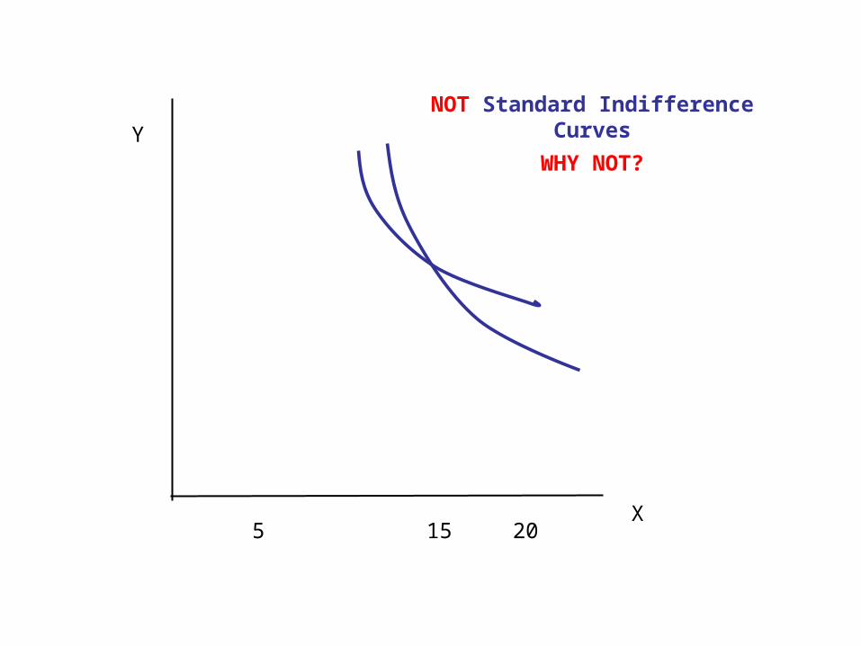
NOT Standard Indifference Curves
WHY NOT?Y
X
5 15 20
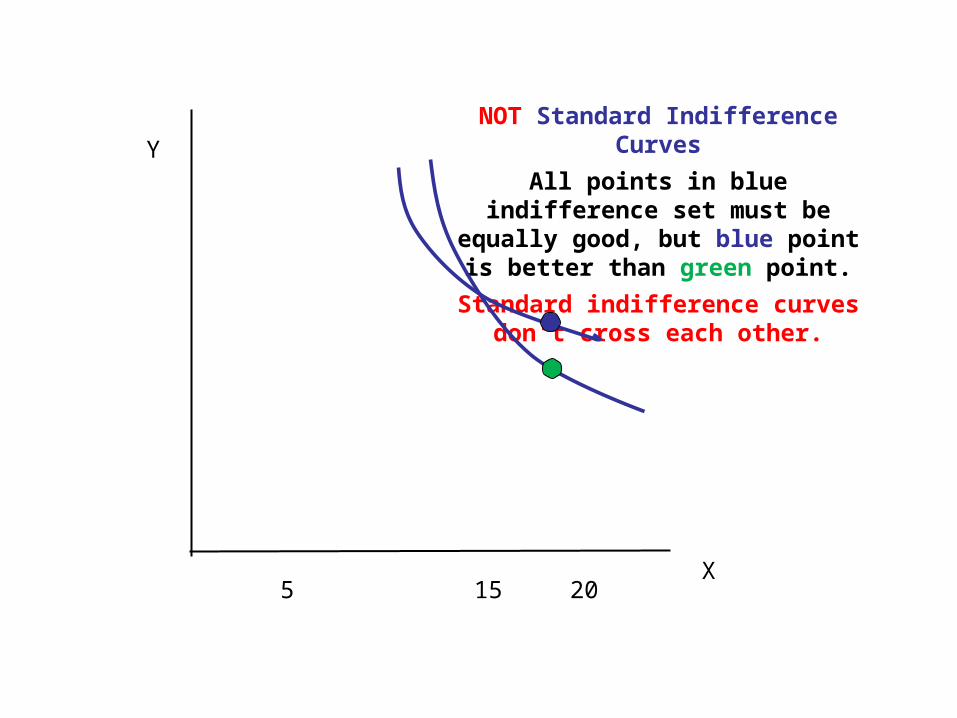
NOT Standard Indifference Curves
All points in blue indifference set must be equally good, but blue point
is better than green point.
Standard indifference curves don't cross each other.
Y
X
5 15 20
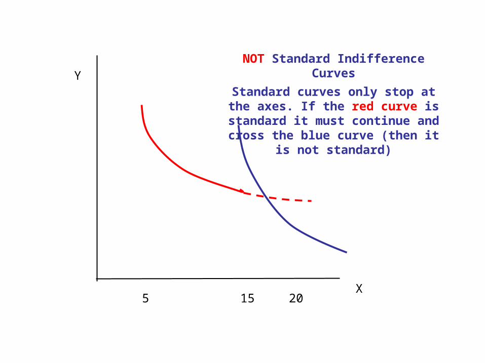
NOT Standard Indifference Curves
Standard curves only stop at the axes. If the red curve is standard it must continue and cross the blue
curve (then it is not standard)
Y
X
5 15 20
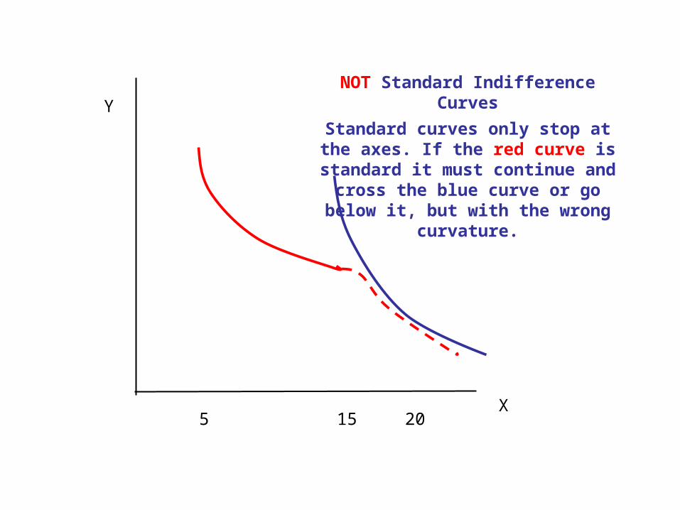
NOT Standard Indifference Curves
Standard curves only stop at the axes. If the red curve is standard it must continue and cross the blue curve or go below it, but with the
wrong curvature.
Y
X
5 15 20
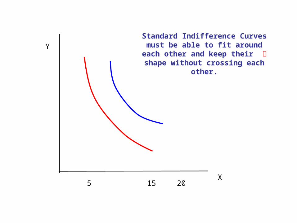
Standard Indifference Curves must be able to fit around each other and keep their shape without crossing
each other.
Y
X
5 15 20
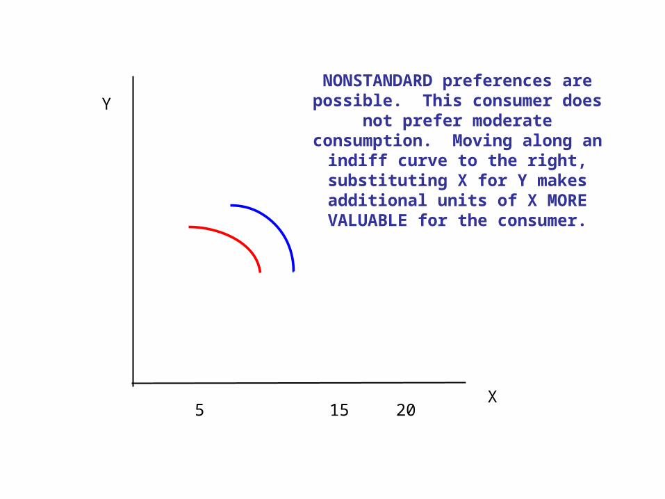
NONSTANDARD preferences are possible. This consumer does not
prefer moderate consumption. Moving along an indiff curve to the
right, substituting X for Y makes additional units of X MORE
VALUABLE for the consumer.
Y
X
5 15 20
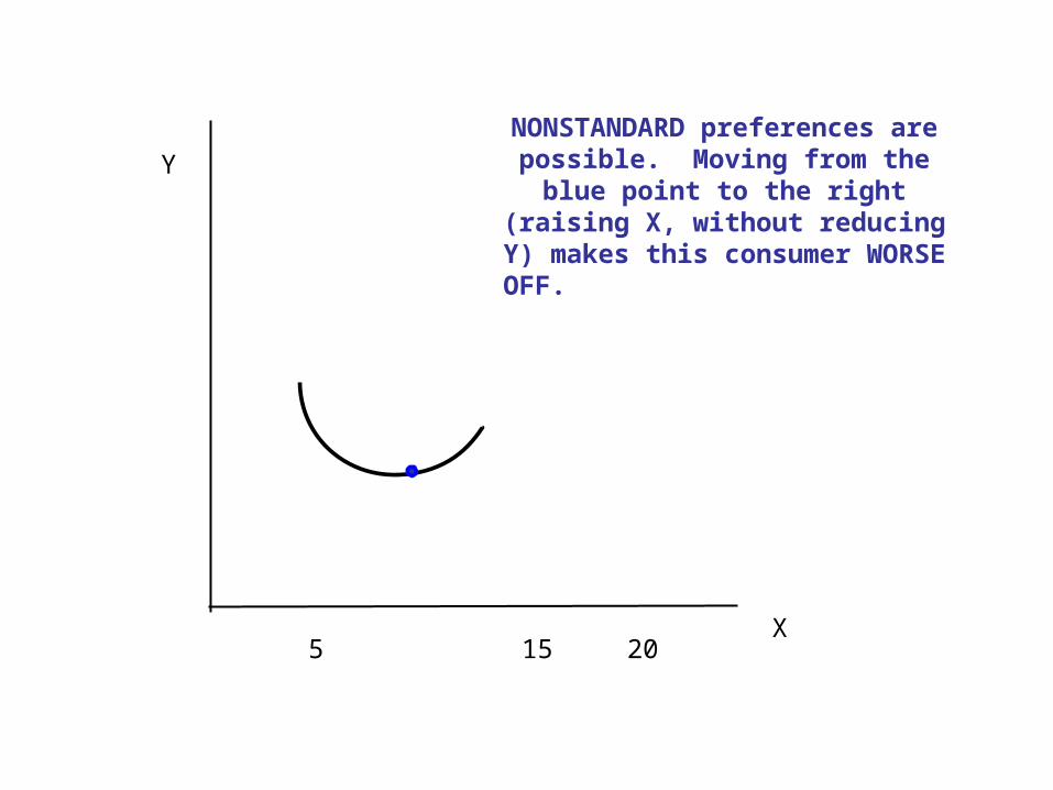
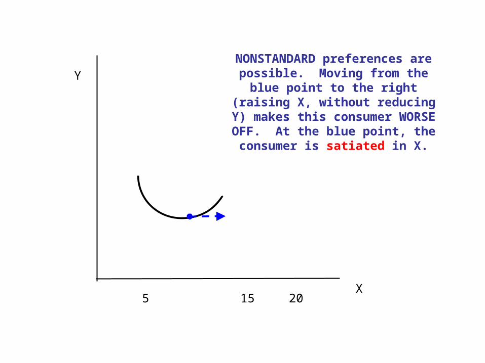
NONSTANDARD preferences are possible. Moving from the blue
point to the right (raising X, without reducing Y) makes this consumer
WORSE OFF. At the blue point, the consumer is satiated in X.
Y
X

5 15 20
NONSTANDARD preferences are possible. Moving from the blue
point to the right (raising X, without reducing Y) makes this consumer
WORSE OFF. At the blue point, the consumer is satiated in X.
Y
X
5 15 20
NONSTANDARD preferences are possible. Moving from the blue
point to the right (raising X, without reducing Y) makes this consumer
WORSE OFF. At the blue point, the consumer is satiated in X.
Y
X
Why Indifference Curves?
Water+Diamond Paradox: Water necessary but free; diamonds unnecessary, expensive.
Prices depend on availability (supply), but why are consumers willing to pay so much more for diamonds?
Answer: Willingness to pay depends on howmuch of ALL goods the consumer starts with.

(5, 15)
(15, 5)
(4,20)
5 15 20
Slope = vertical change / horizontal change
= (20−15) / (4 −5) = −5/1
Starting at black point, with a lot of diamonds and little water, consumer is willing to pay a lot for one more unit of
water.
Diamonds
Water
(5, 15)
(15, 5)
(4,20)
5 15 20
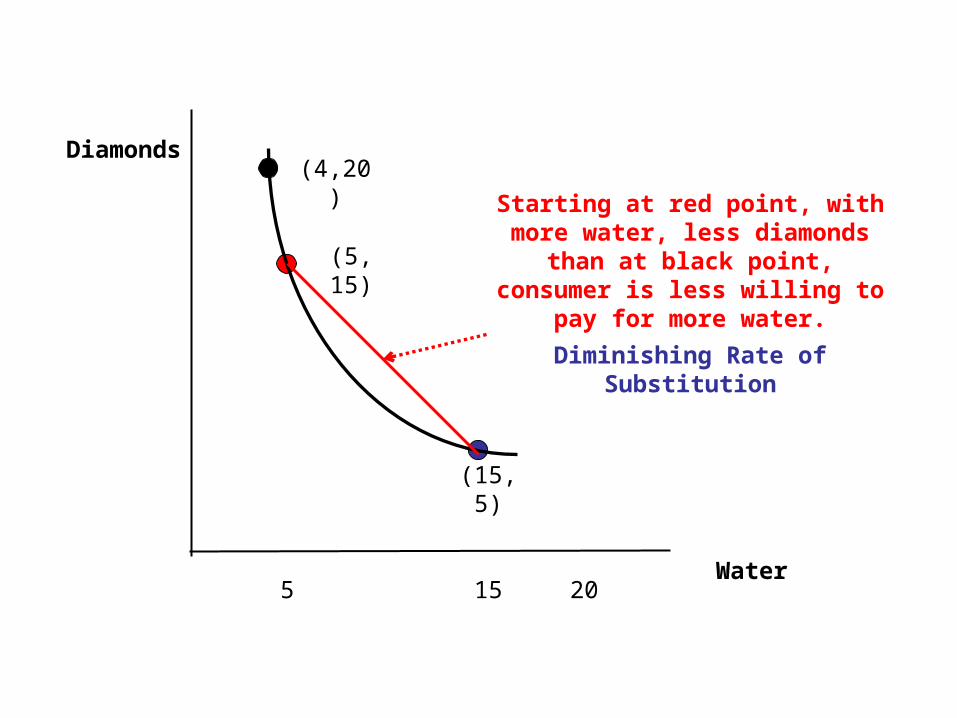
Starting at red point, with more water, less diamonds than at black point, consumer is less willing to pay for more water.
Diminishing Rate of Substitution
Diamonds
Water
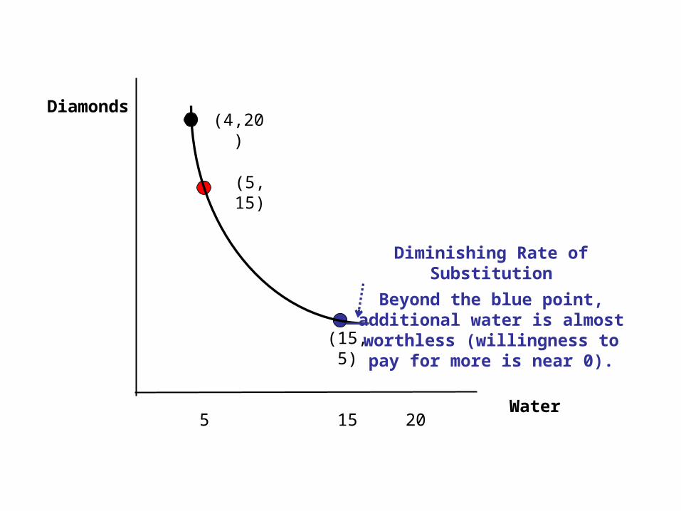
(5, 15)
(15, 5)
(4,20)
5 15 20
Starting at blue point, with more water, less diamonds, consumer
is willing to pay less for more water.
Diminishing Rate of Substitution
Beyond the blue point, additional water is almost worthless
(willingness to pay for more is near 0).
Diamonds
Water
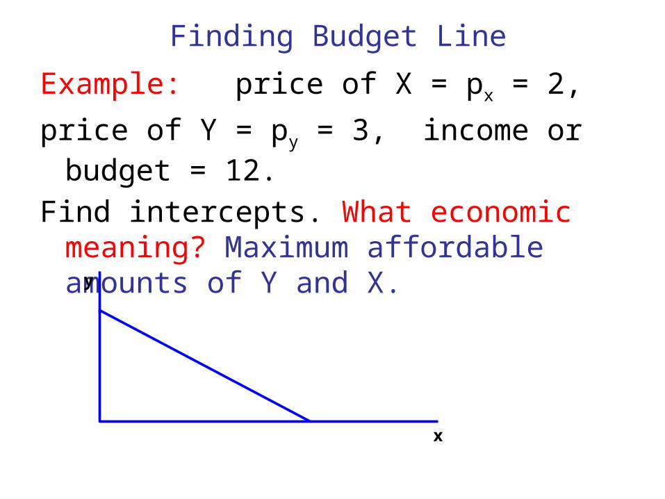
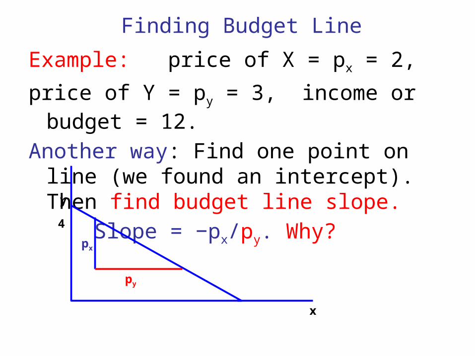
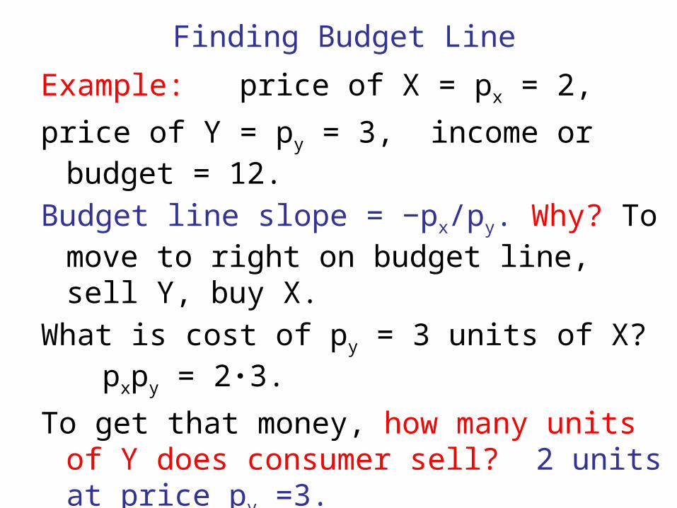
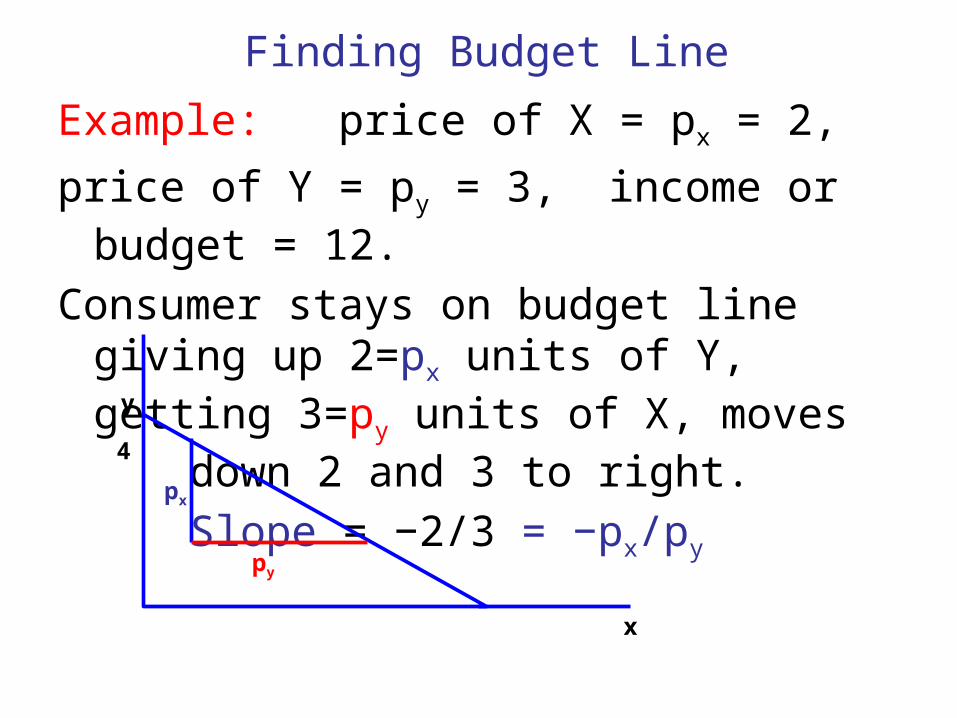
Finding Budget Line
Example: price of X = px = 2,
price of Y = py = 3, income or budget = 12.
Find intercepts. What economic meaning? Maximum affordable amounts of Y and X.
y
x
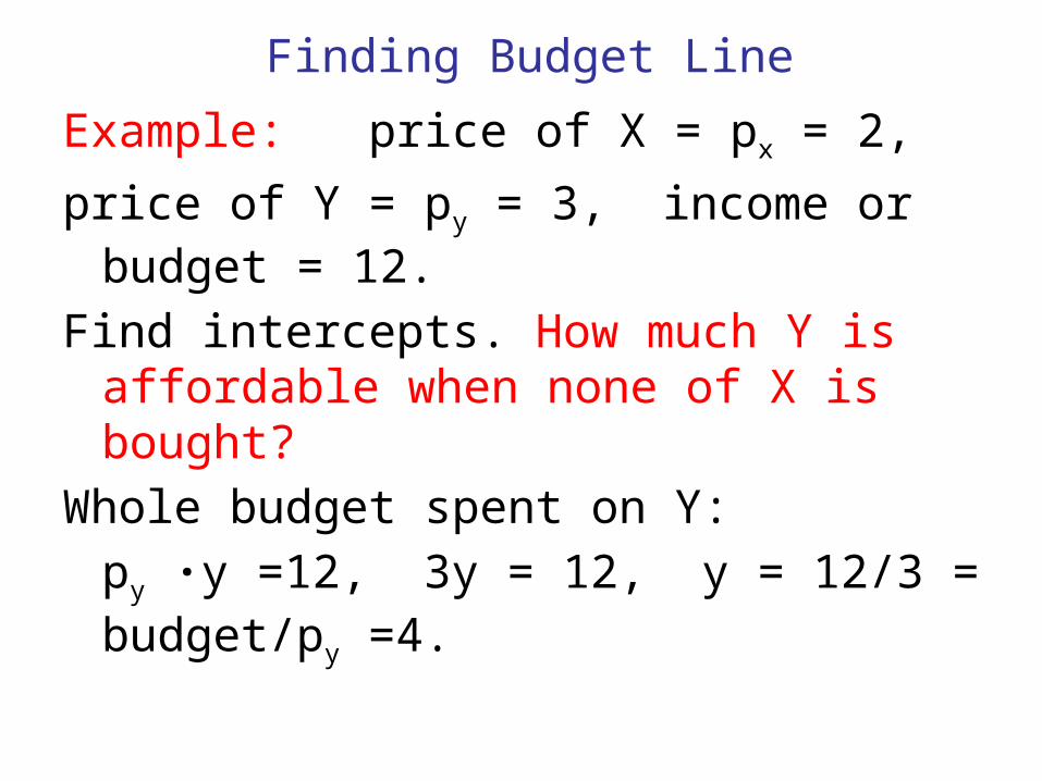
Finding Budget Line
Example: price of X = px = 2,
price of Y = py = 3, income or budget = 12.
Find intercepts. How much Y is affordable when none of X is bought?
Whole budget spent on Y:
py ∙y =12, 3y = 12, y = 12/3 = budget/py =4.
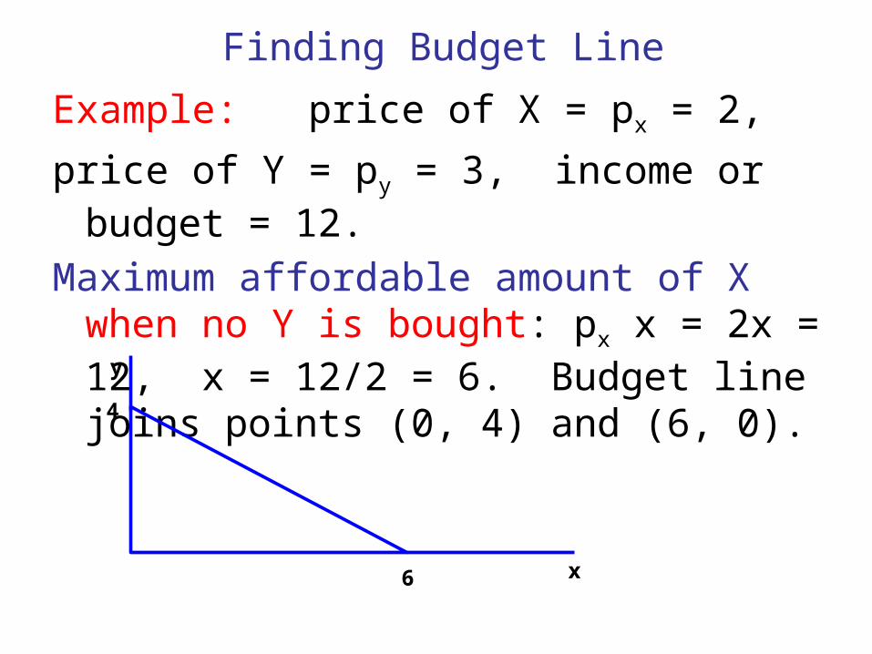
Finding Budget Line
Example: price of X = px = 2,
price of Y = py = 3, income or budget = 12.
Maximum affordable amount of X when no Y is bought: px x = 2x = 12, x = 12/2 = 6. Budget line joins points (0, 4) and (6, 0).
4
y
x6
Finding Budget Line
Example: price of X = px = 2,
price of Y = py = 3, income or budget = 12.
Another way: Find one point on line (we found an intercept). Then find budget line slope.
Slope = −px/py. Why?
4
y
x
px
py
Finding Budget Line
Example: price of X = px = 2,
price of Y = py = 3, income or budget = 12.
Budget line slope = −px/py. Why? To move to right on budget line, sell Y, buy X.
What is cost of py = 3 units of X? pxpy = 2∙3.
To get that money, how many units of Y does consumer sell? 2 units at price py =3.
Gives up 2 of Y to get 3 of X. Moves down 2 and 3 to right. Slope = −2/3 = −px/py
Finding Budget Line
Example: price of X = px = 2,
price of Y = py = 3, income or budget = 12.
Consumer stays on budget line giving up 2=px units of Y, getting 3=py units of X, moves
down 2 and 3 to right.
Slope = −2/3 = −px/py4
y
x
px
py
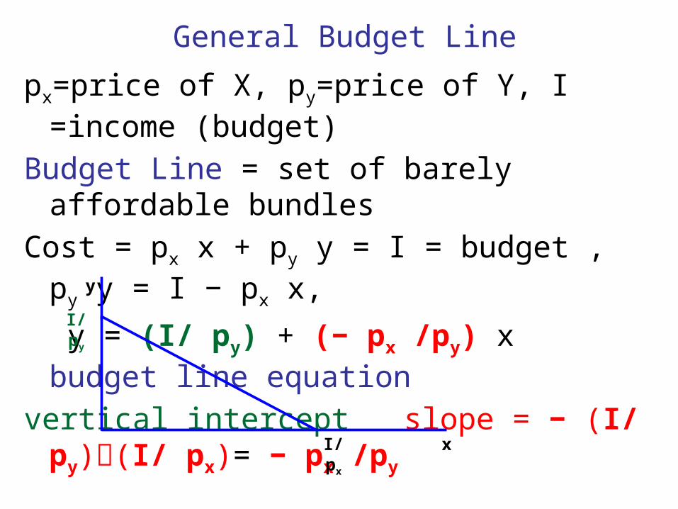
General Budget Line
px=price of X, py=price of Y, I =income (budget)
Budget Line = set of barely affordable bundles
Cost = px x + py y = I = budget , py y = I − px x,
y = (I/ py) + (− px /py) x budget line equation
vertical intercept slope = − (I/ py)(I/ px)= − px /py
I/ py
y
xI/ px
Effects of Income Changes
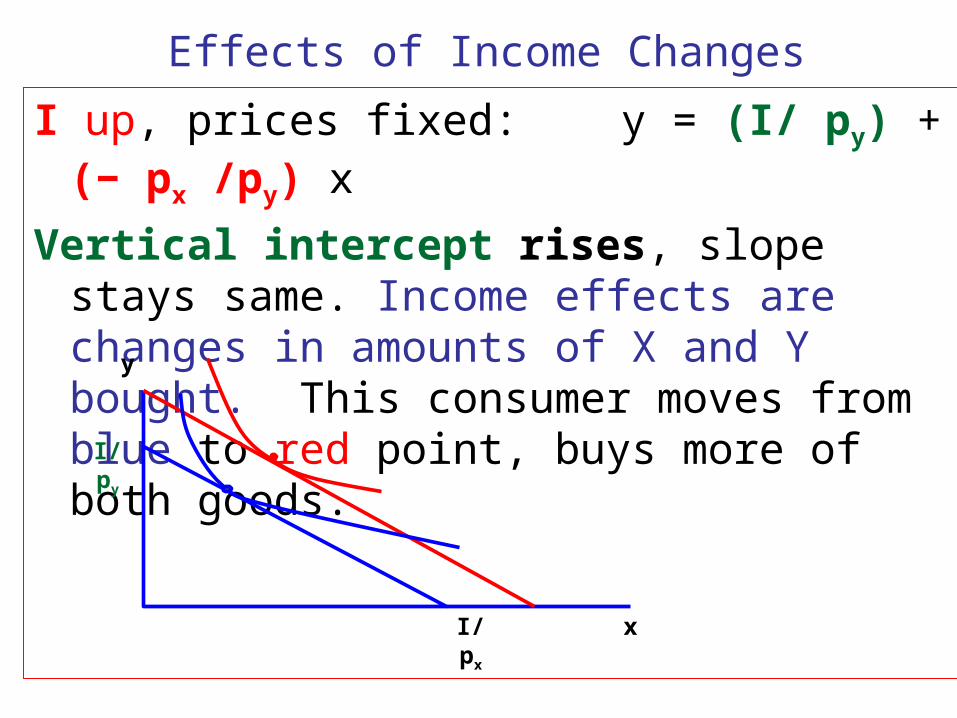
I up, prices fixed: y = (I/ py) + (− px /py) x
Vertical intercept rises, slope stays same. Income effects are changes in amounts of X and Y bought. This consumer moves from blue to red point, buys more of both goods.
I/ py
y
xI/ px
Effects of Income Changes
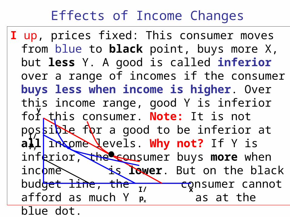
I up, prices fixed: This consumer moves from blue to black point, buys more X, but less Y. A good is called inferior over a range of incomes if the consumer buys less when income is higher. Over this income range, good Y is inferior for this consumer. Note: It is not possible for a good to be inferior at all income levels. Why not? If Y is
inferior, the consumer buys more when income is lower. But on the black budget line, the consumer cannot afford as much Y as at the blue dot.
I/ py
y
xI/ px
Effects of Income Changes
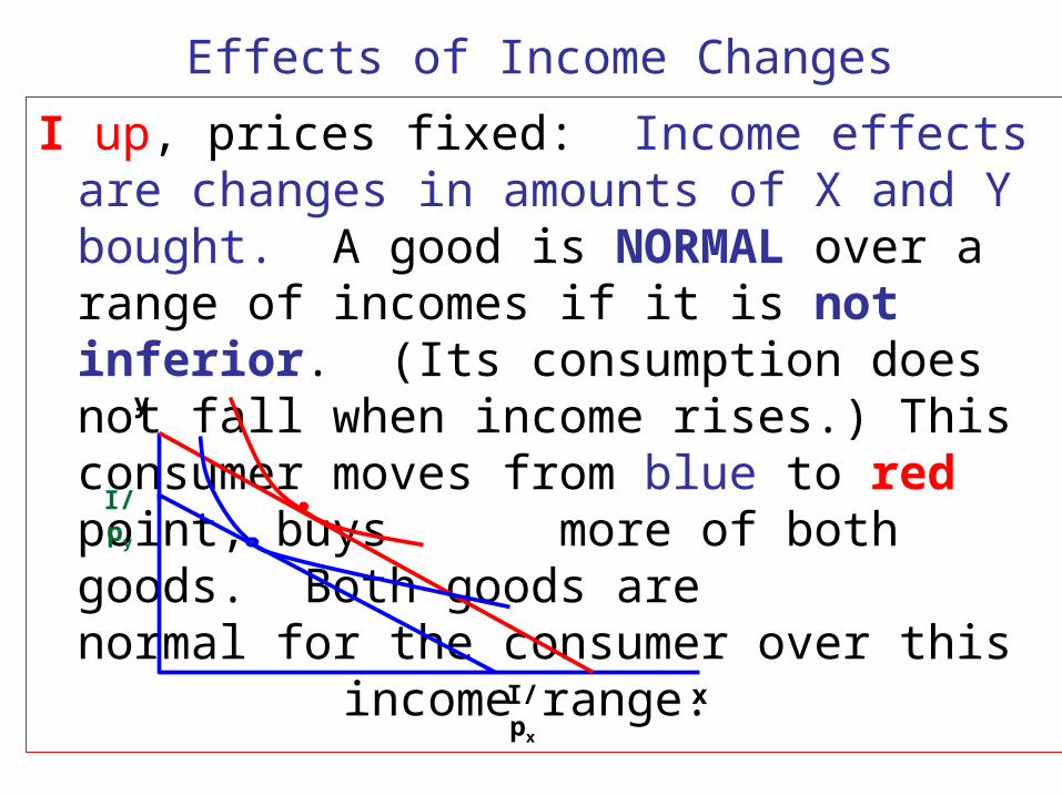
I up, prices fixed: Income effects are changes in amounts of X and Y bought. A good is NORMAL over a range of incomes if it is not inferior. (Its consumption does not fall when income rises.) This consumer moves from blue to red point, buys
more of both goods. Both goods are normal for the consumer over this
income range.I/ py
y
xI/ px
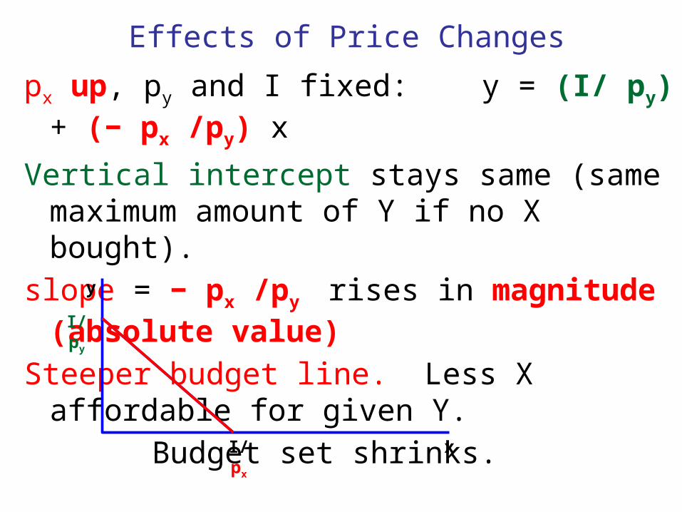
Effects of Price Changes
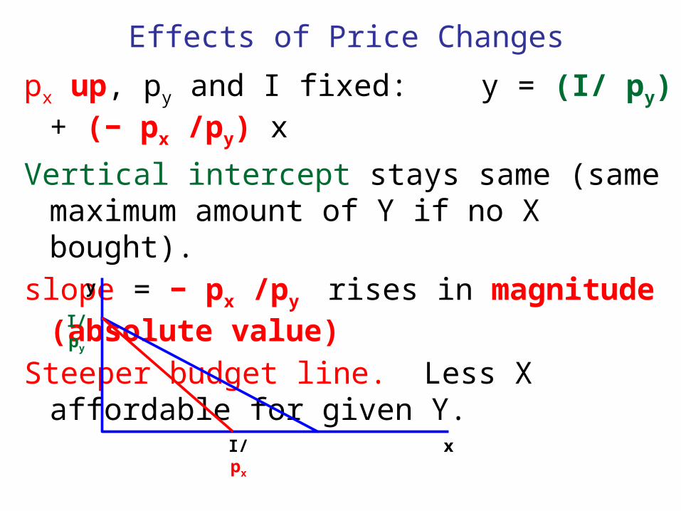
px up, py and I fixed: y = (I/ py) + (− px /py) x
Vertical intercept stays same (same maximum amount of Y if no X bought).
slope = − px /py rises in magnitude (absolute value)
Steeper budget line. Less X affordable for given Y.
I/ py
y
xI/ px
Effects of Price Changes
px up, py and I fixed: y = (I/ py) + (− px /py) x
Vertical intercept stays same (same maximum amount of Y if no X bought).
slope = − px /py rises in magnitude (absolute value)
Steeper budget line. Less X affordable for given Y.
Budget set shrinks.I/ py
y
xI/ px
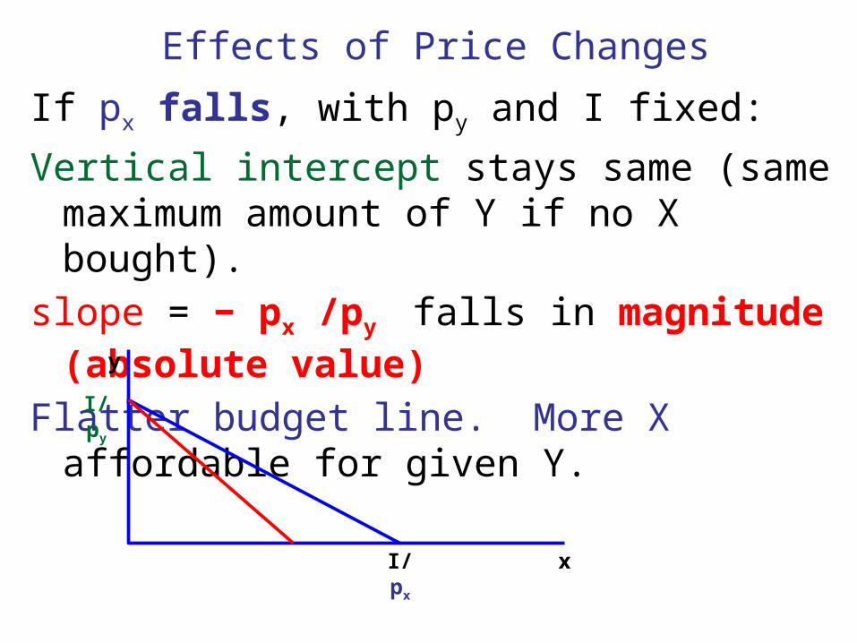
Effects of Price Changes
If px falls, with py and I fixed:
Vertical intercept stays same (same maximum amount of Y if no X bought).
slope = − px /py falls in magnitude (absolute value)
Flatter budget line. More X affordable for given Y.
I/ py
y
xI/ px
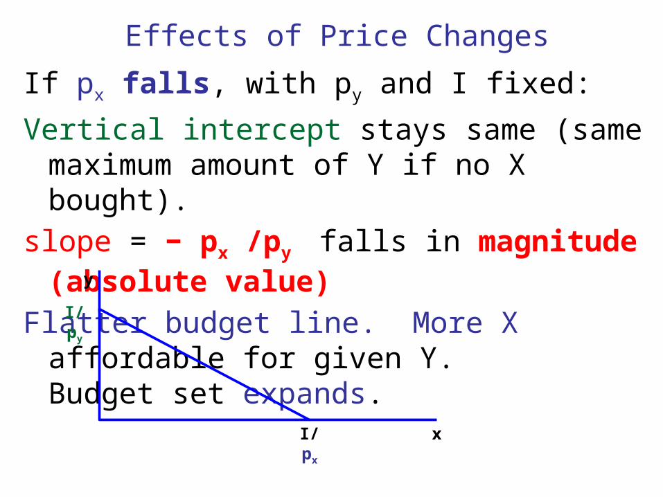
Effects of Price Changes
If px falls, with py and I fixed:
Vertical intercept stays same (same maximum amount of Y if no X bought).
slope = − px /py falls in magnitude (absolute value)
Flatter budget line. More X affordable for given Y. Budget set expands.
I/ py
y
xI/ px
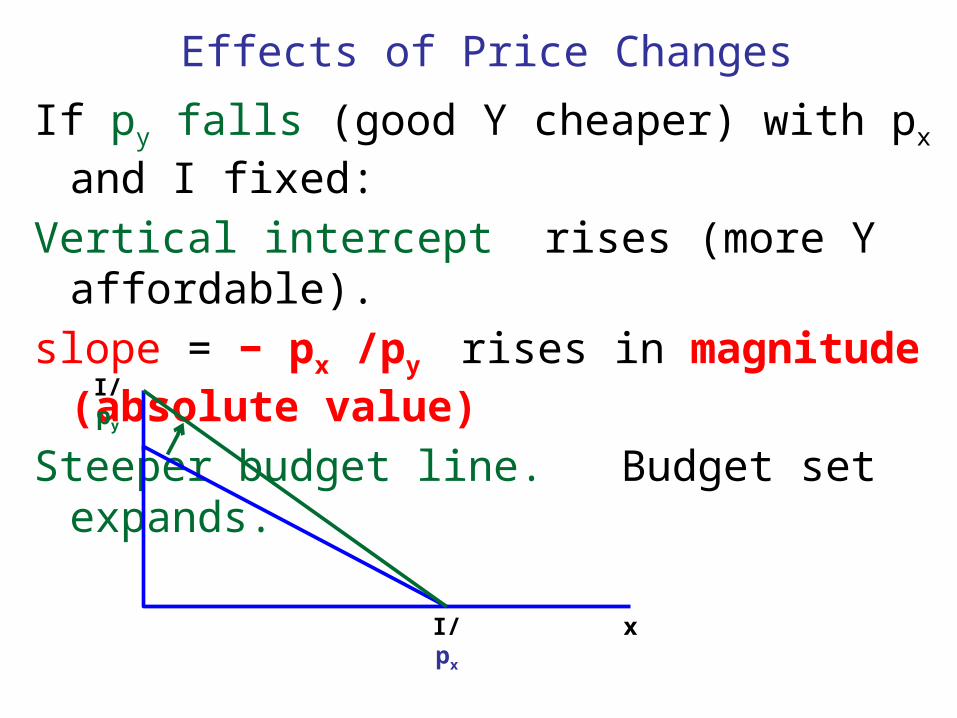
Effects of Price Changes
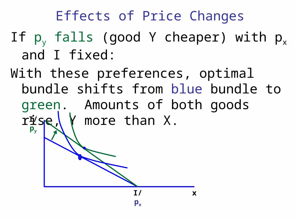
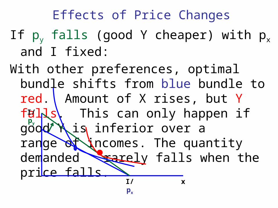
If py falls (good Y cheaper) with px and I fixed:
Vertical intercept rises (more Y affordable).
slope = − px /py rises in magnitude (absolute value)
Steeper budget line. Budget set expands.
I/ py
xI/ px
Effects of Price Changes
If py falls (good Y cheaper) with px and I fixed:
With these preferences, optimal bundle shifts from blue bundle to green. Amounts of both goods rise, Y more than X.
I/ py
xI/ px
Effects of Price Changes
If py falls (good Y cheaper) with px and I fixed:
With other preferences, optimal bundle shifts from blue bundle to red. Amount of X rises, but Y falls. This can only happen if good Y is inferior over a range of incomes. The quantity demanded
rarely falls when the price falls.I/ py
xI/ px
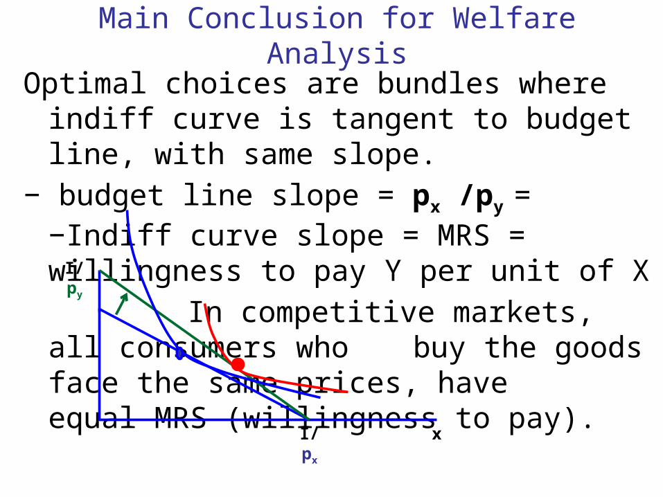
Main Conclusion for Welfare Analysis
Optimal choices are bundles where indiff curve is tangent to budget line, with same slope.
− budget line slope = px /py = −Indiff curve slope = MRS = willingness to pay Y per unit of X
In competitive markets, all consumers who buy the goods face the same prices, have equal MRS (willingness to pay).
I/ py
xI/ px

Kinked Budget Lines: Labor Supply with TANF Benefits
Indifference curves usually represent preferences for desirable goods. We use leisure (desirable) instead of labor to study labor supply. Consider a consumer who can work any number of hour up to full time in a year at wage rate $10/hour. Full time = 40 hours/week for 50 weeks = 2000 hours/yr.
Any hours out of the 2000 not spent working are counted as leisure consumption:
Work time + Leisure time = 2000 hrs.
We will consider the effect of TANF welfare benefits (Temporary Assistance for Needy Families) on a consumer's budget set and choice of labor supply.
Kinked Budget Lines: Labor Supply with TANF benefits
$ for other goods
leisure
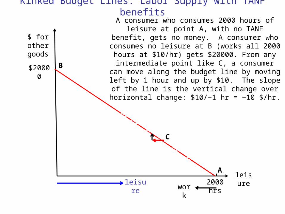
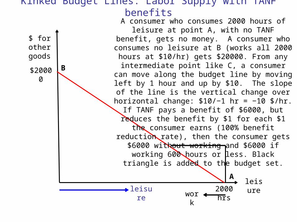
A consumer who consumes 2000 hours of leisure at point A, with no TANF benefit, gets no money. A consumer who
consumes no leisure at B (works all 2000 hours at $10/hr) gets $20000. From any intermediate point like C, a
consumer can move along the budget line by moving left by 1 hour and up by $10. The slope of the line is the vertical change over horizontal change: $10/−1 hr = −10 $/hr. If
TANF pays a benefit of $6000, but reduces the benefit by $1 for each $1 the consumer earns (100% benefit reduction rate), then the consumer gets $6000 without working and
$6000 if working 600 hours or less. The budget set expands
2000 hrs
$20000
A
B
work
leisure
C
Kinked Budget Lines: Labor Supply with TANF benefits
$ for other goods
leisure
A consumer who consumes 2000 hours of leisure at point A, with no TANF benefit, gets no money. A consumer who
consumes no leisure at B (works all 2000 hours at $10/hr) gets $20000. From any intermediate point like C, a
consumer can move along the budget line by moving left by 1 hour and up by $10. The slope of the line is the vertical change over horizontal change: $10/−1 hr = −10 $/hr. If
TANF pays a benefit of $6000, but reduces the benefit by $1 for each $1 the consumer earns (100% benefit reduction rate), then the consumer gets $6000 without working and
$6000 if working 600 hours or less. Black triangle is added to the budget set.
2000 hrs
$20000
A
B
work
leisure
Kinked Budget Lines: Labor Supply with TANF benefits
$ for other goods
leisure
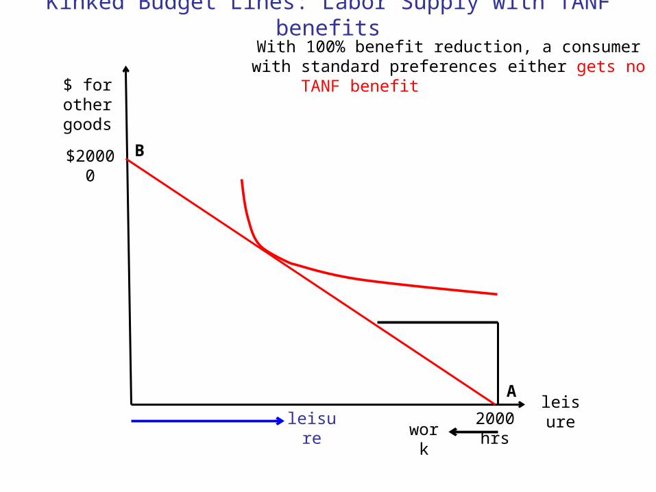
With 100% benefit reduction, a consumer with standard preferences either gets no TANF benefit or does not work.
2000 hrs
$20000
A
B
work
leisure

Kinked Budget Lines: Labor Supply with TANF benefits
$ for other goods
leisure
With 100% benefit reduction, a consumer with standard preferences either gets no TANF benefit or does not work.
2000 hrs
$20000
A
B
work
leisure
Kinked Budget Lines: Labor Supply with TANF benefits
$ for other goods
leisure
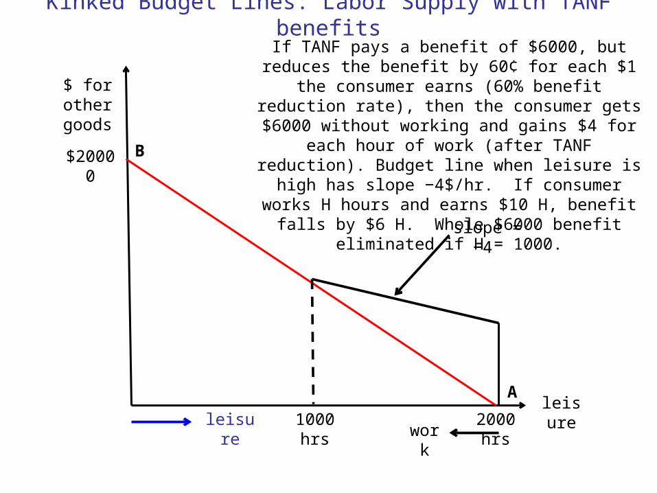
If TANF pays a benefit of $6000, but reduces the benefit by 60¢ for each $1 the consumer earns (60% benefit reduction rate), then the consumer gets $6000 without working and gains $4 for each hour of work (after TANF reduction). Budget line when leisure is high has slope −4$/hr. If
consumer works H hours and earns $10 H, benefit falls by $6 H. Whole $6000 benefit eliminated if H = 1000.
2000 hrs
$20000
A
B
work
leisure1000 hrs
slope = −4
Kinked Budget Lines: Labor Supply with TANF benefits
$ for other goods
leisure
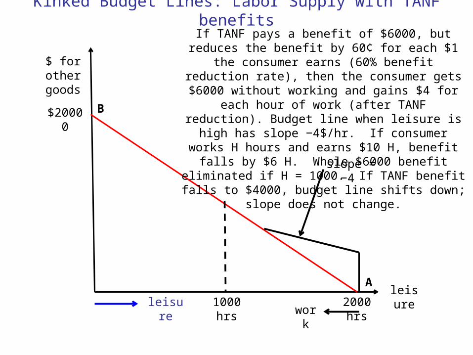
If TANF pays a benefit of $6000, but reduces the benefit by 60¢ for each $1 the consumer earns (60% benefit reduction rate), then the consumer gets $6000 without working and gains $4 for each hour of work (after TANF reduction). Budget line when leisure is high has slope −4$/hr. If
consumer works H hours and earns $10 H, benefit falls by $6 H. Whole $6000 benefit eliminated if H = 1000. If
TANF benefit falls to $4000, budget line shifts down; slope does not change.
2000 hrs
$20000
A
B
work
leisure1000 hrs
slope = −4
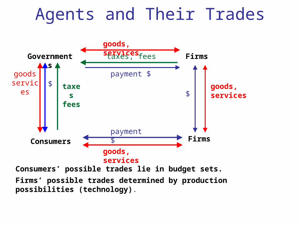
Agents and Their Trades
Consumers
Firms
Firmspayment $
goods, services
goods, services
payment $
$goods, services
Consumers’ possible trades lie in budget sets.
Firms’ possible trades determined by production possibilities (technology).
Governments taxes, fees
goodsservices $ taxes
fees
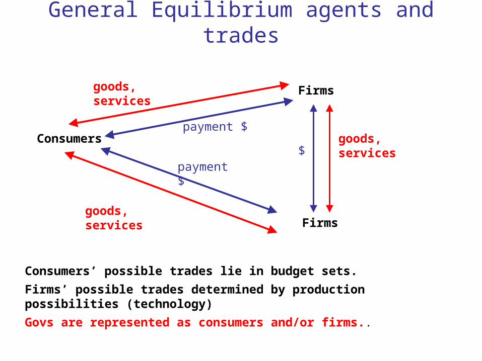
General Equilibrium agents and trades
Consumers
Firms
Firms
payment $
goods, services
goods, services
payment $
$goods, services
Consumers’ possible trades lie in budget sets.
Firms’ possible trades determined by production possibilities (technology)
Govs are represented as consumers and/or firms..
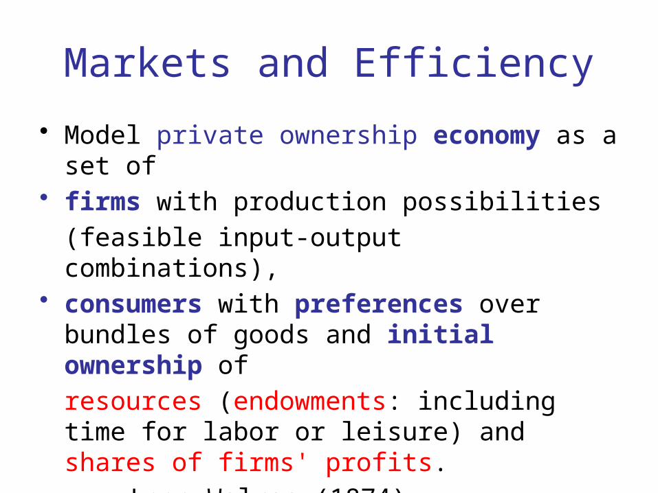
Markets and Efficiency
• Model private ownership economy as a set of• firms with production possibilities
(feasible input-output combinations),• consumers with preferences over bundles of
goods and initial ownership of
resources (endowments: including time for labor or leisure) and shares of firms' profits.
Leon Walras (1874)
5 15 20
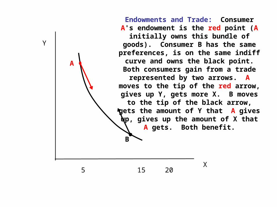
Endowments and Trade: Consumer A's endowment is the red point (A initially
owns this bundle of goods). Consumer B has the same preferences, is on the same
indiff curve and owns the black point. Both consumers gain from a trade represented by two arrows. A moves to the tip of the
red arrow, gives up Y, gets more X. B moves to the tip of the black arrow, gets
the amount of Y that A gives up, gives up the amount of X that A gets. Both benefit.
Y
X
A
B
5 15 20
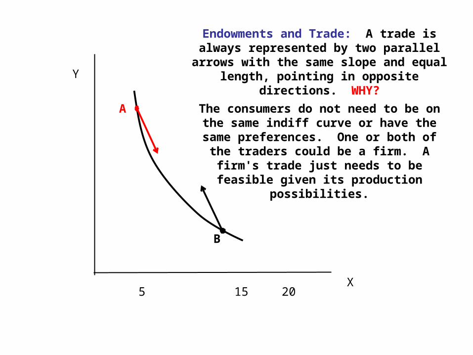
Endowments and Trade: A trade is always represented by two parallel arrows with the
same slope and equal length, pointing in opposite directions. WHY?
The consumers do not need to be on the same indiff curve or have the same
preferences. One or both of the traders could be a firm. A firm's trade just needs to be
feasible given its production possibilities.
Y
X
A
B

• Allocation: amount of each good for each consumer, and amount of each input and each output for each firm.
• Feasible allocation:
For each good,
total demand by consumers and firms
= total output + total (initial) endowment.
= total supply.
Competitive Equilibrium (CE)• Prices for all goods
(in single market, goods are identical);• Competitive behavior:
Firms price-taking profit maximizers; Consumers price-taking optimizers,
value of net trade equals profit share.• Feasible allocation: prices adjust so
supply = demand for each good.

Graded Homework 1, problem 1
Define "market" broadly enough to cover market for wheat, U.S. anesthesiologists, and for a particular stock.
• Market changes when essential features change and only then. What is wrong with:
A "collection of buyers and sellers that, through their actual or potential interactions, determine the price of a product or set of products." ?
.
Efficient allocation (W. Pareto, 1906):Think first about what is inefficient.
• An allocation is INEFFICIENT if some feasible allocation is better for some consumer and no worse for anyone.
Pareto improvement makes at least one consumer better off without hurting anyone
• Efficient = feasible and not inefficient.• A feasible allocation is (Pareto) efficient if
no Pareto improvement is feasible. (It is impossible to make a consumer better off without hurting someone else.)
• We care only about consumer welfare.• Care about firms indirectly
(care about their owners).• Efficient is NOT same as desirable.
An efficient allocation may be very unfair.• Example: all goods to one person.

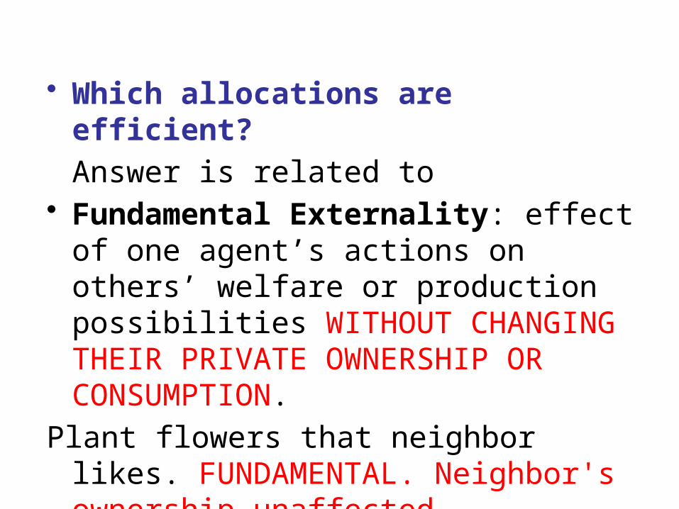
• Which allocations are efficient?
Answer is related to• Fundamental Externality: effect of one
agent’s actions on others’ welfare or production possibilities WITHOUT CHANGING THEIR PRIVATE OWNERSHIP OR CONSUMPTION.
Oil spill makes fishing more difficult (need to sail farther). FUNDAMENTAL: affects production possibilities.
• Which allocations are efficient?
Answer is related to• Fundamental Externality: effect of one
agent’s actions on others’ welfare or production possibilities WITHOUT CHANGING THEIR PRIVATE OWNERSHIP OR CONSUMPTION.
Plant flowers that neighbor likes. FUNDAMENTAL. Neighbor's ownership unaffected.

• Which allocations are efficient?
Answer is related to• Fundamental Externality: effect of one
agent’s actions on others’ welfare or production possibilities WITHOUT CHANGING THEIR PRIVATE OWNERSHIP OR CONSUMPTION.
Apple introduces iPad, reducing Amazon Kindle profit. NOT FUNDAMENTAL.
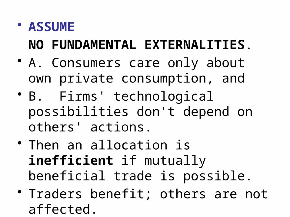
• ASSUME
NO FUNDAMENTAL EXTERNALITIES.• A. Consumers care only about own private
consumption, and• B. Firms' technological possibilities don't
depend on others' actions.• Then an allocation is inefficient if mutually
beneficial trade is possible.• Traders benefit; others are not affected.
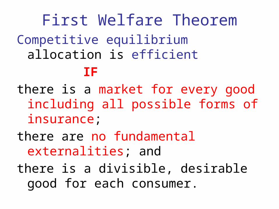
First Welfare TheoremCompetitive equilibrium allocation is efficient
IF
there is a market for every good including all possible forms of insurance;
there are no fundamental externalities; and
there is a divisible, desirable good for each consumer.
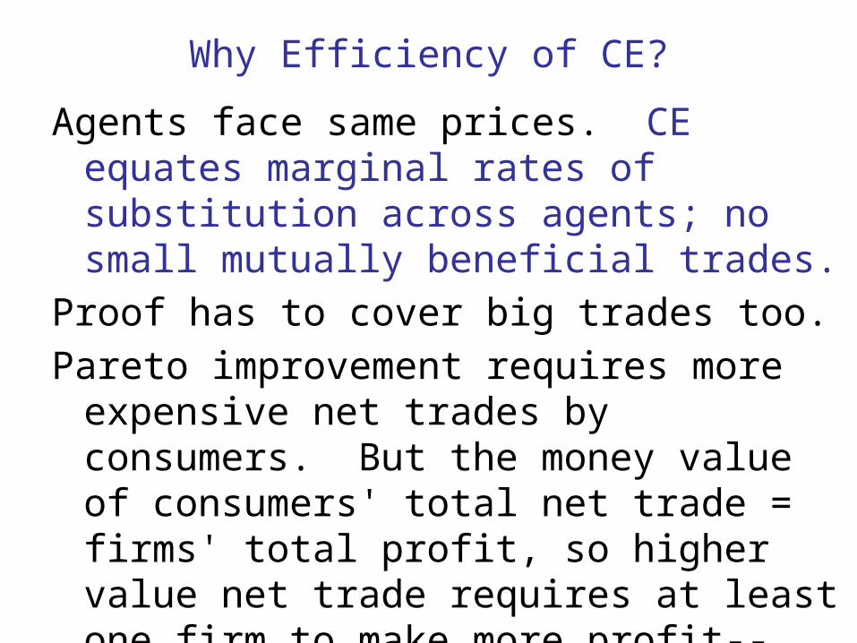
Why Efficiency of CE?
Agents face same prices. CE equates marginal rates of substitution across agents; no small mutually beneficial trades.
Proof has to cover big trades too.
Pareto improvement requires more expensive net trades by consumers. But the money value of consumers' total net trade = firms' total profit, so higher value net trade requires at least one firm to make more profit--impossible if it is already maximizing profit.
Welfare Theorem does NOT say free markets yield efficient allocation.
Potential Problems
Noncompetitive behavior
Inefficient externalities (fundamental or not).
Welfare Theorem does NOT say free markets yield efficient allocation.
Potential Problems1. Noncompetitive Behavior
Market power: Traders take account of their effect on prices (oligopoly, unions,...).
Theft, violence, sabotage, ...
Consumers do not stay in budget sets;
Firms break contracts, sabotage rivals.
Nonrational behavior or other goals.

Potential Problems2. Fundamental Externalities
environmental, technological,empathy, status concerns, envy, ... .
3. Asymmetric information about qualityTheorem assumes identical goods in each market; BUT some firms sell junk;some workers shirk.
Still can get efficiency if qualities differ, but agents don’t notice or don’t care.
First theorem does not sayIf all producers and consumers act as perfect
competitors and a market exists for every commodity, with no fundamental externalities, efficient allocation emerges.
WHY NOT?
a. Competitive equilibrium may not exist.
Can’t exist with significant increasing returns.
b. Equilibrium may not be reached:
optimism, pessimism; prices overshoot.
Anything possible in model, Sonnenschein '73
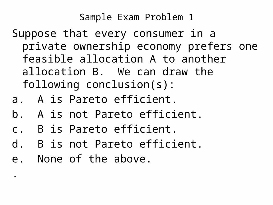
Sample Exam Problem 1
Suppose that every consumer in a private ownership economy prefers one feasible allocation A to another allocation B. We can draw the following conclusion(s):
a. A is Pareto efficient.
b. A is not Pareto efficient.
c. B is Pareto efficient.
d. B is not Pareto efficient.
e. None of the above.
.
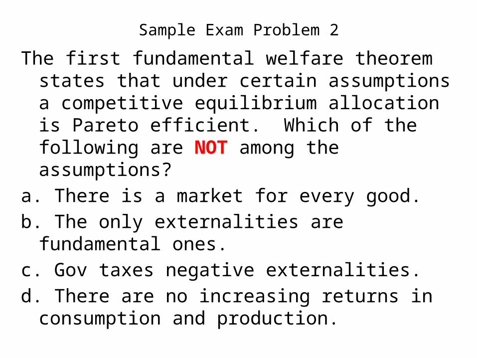
Sample Exam Problem 2
The first fundamental welfare theorem states that under certain assumptions a competitive equilibrium allocation is Pareto efficient. Which of the following are NOT among the assumptions?
a. There is a market for every good.
b. The only externalities are fundamental ones.
c. Gov taxes negative externalities.
d. There are no increasing returns in consumption and production.
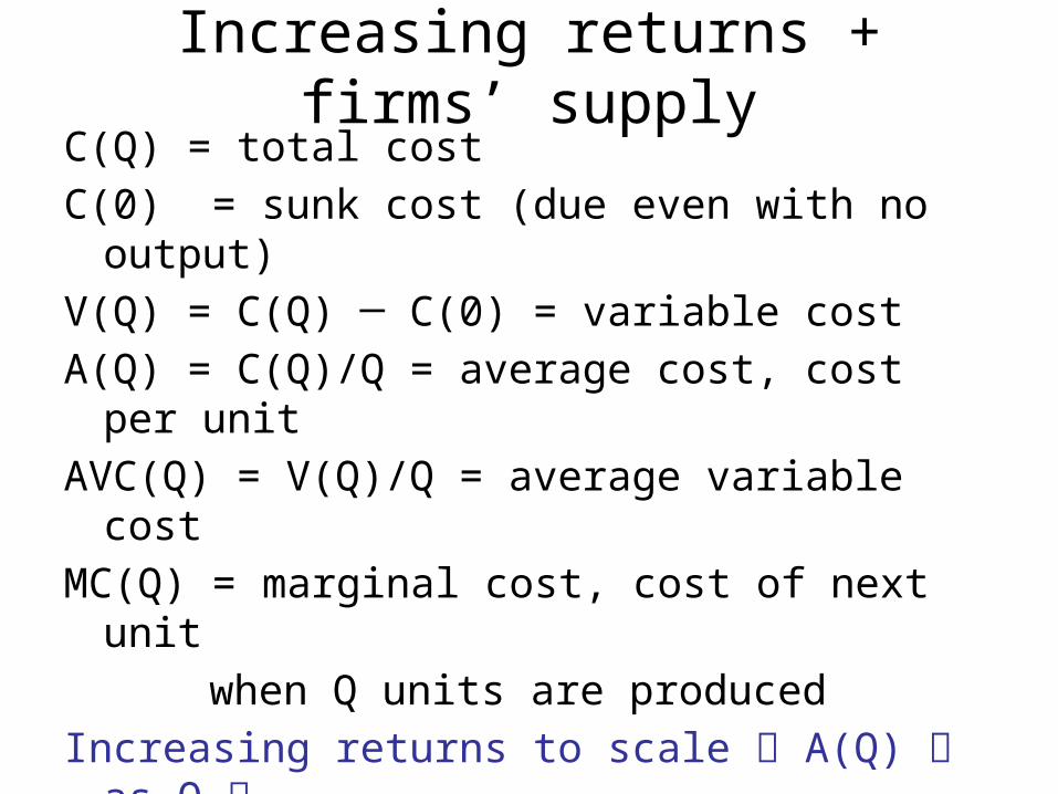
Increasing returns + firms’ supplyC(Q) = total cost
C(0) = sunk cost (due even with no output)
V(Q) = C(Q) ─ C(0) = variable cost
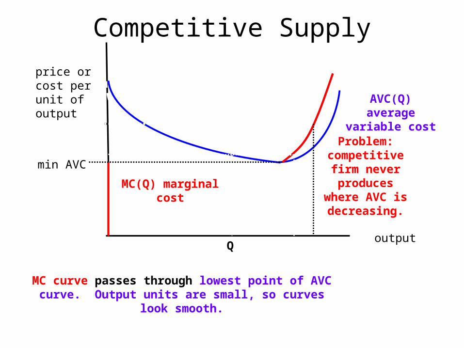
A(Q) = C(Q)/Q = average cost, cost per unit
AVC(Q) = V(Q)/Q = average variable cost
MC(Q) = marginal cost, cost of next unit
when Q units are produced
Increasing returns to scale A(Q) as Q A(Q) > MC(Q) marginal cost below ave.
Marginal cost pulls average down.

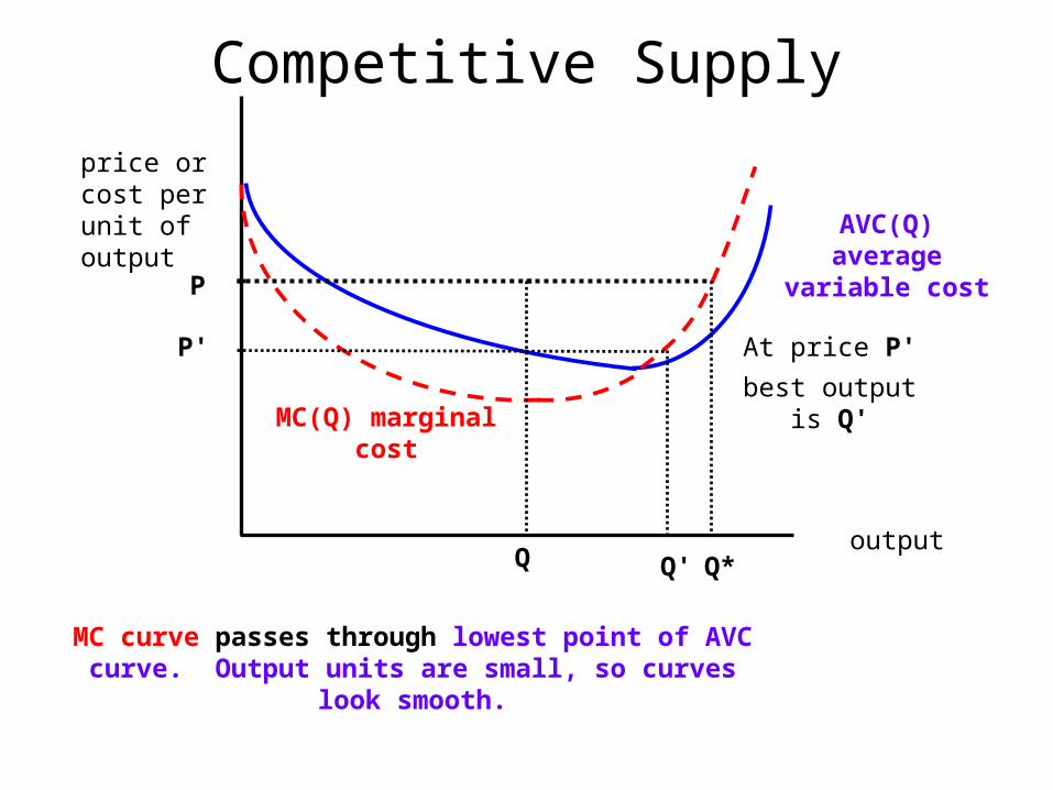
Competitive Supply
output
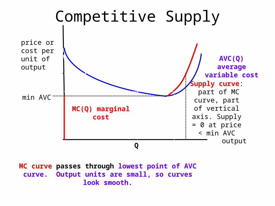
price or cost per unit of output AVC(Q) average
variable cost
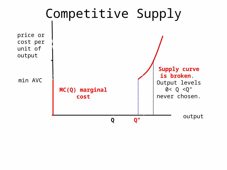
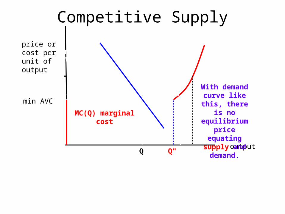
MC(Q) marginal cost
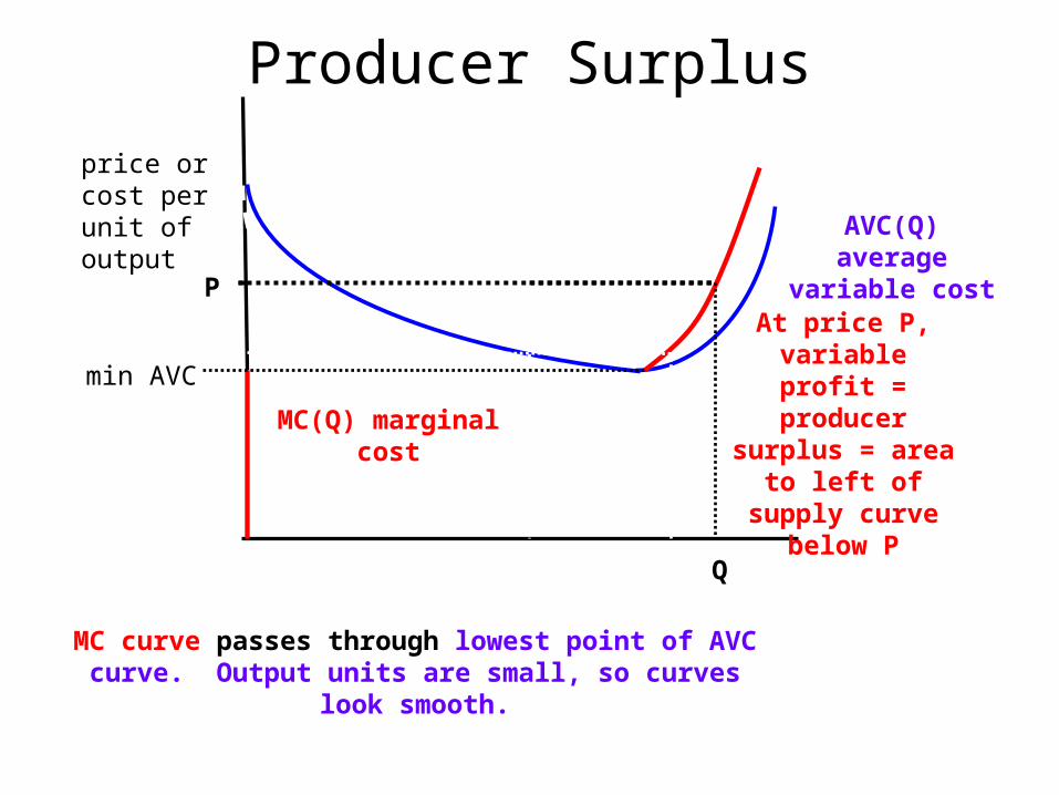
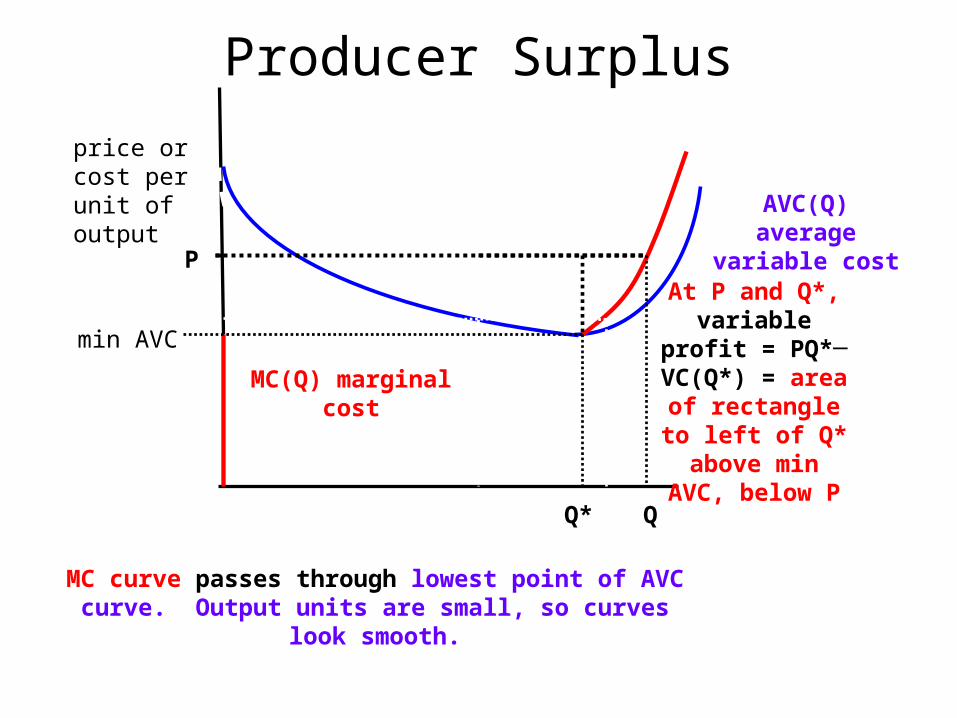
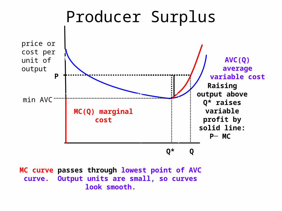
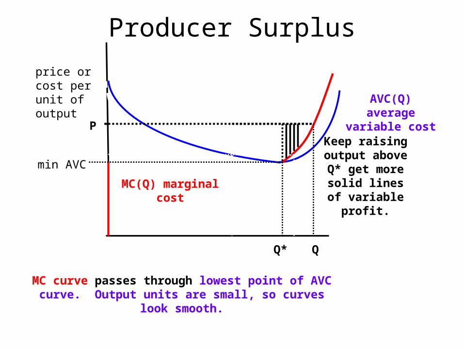
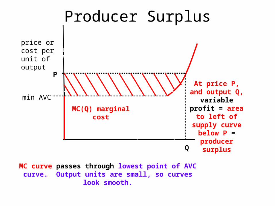
MC curve passes through lowest point of AVC curve. Output units are small, so curves look smooth.
P
Q
At output level Q,raising output
raises profit since P > MC(Q)

Competitive Supply
output
price or cost per unit of output AVC(Q) average
variable cost
MC(Q) marginal cost
MC curve passes through lowest point of AVC curve. Output units are small, so curves look smooth.
P
Q
Raising output beyond Q*
reduces profit:
P<MC(Q) if Q>Q*
Q*
Competitive Supply
output
price or cost per unit of output AVC(Q) average
variable cost
MC(Q) marginal cost
MC curve passes through lowest point of AVC curve. Output units are small, so curves look smooth.
P
Q
At price P'
best output is Q'
Q*
P'
Q'
P"
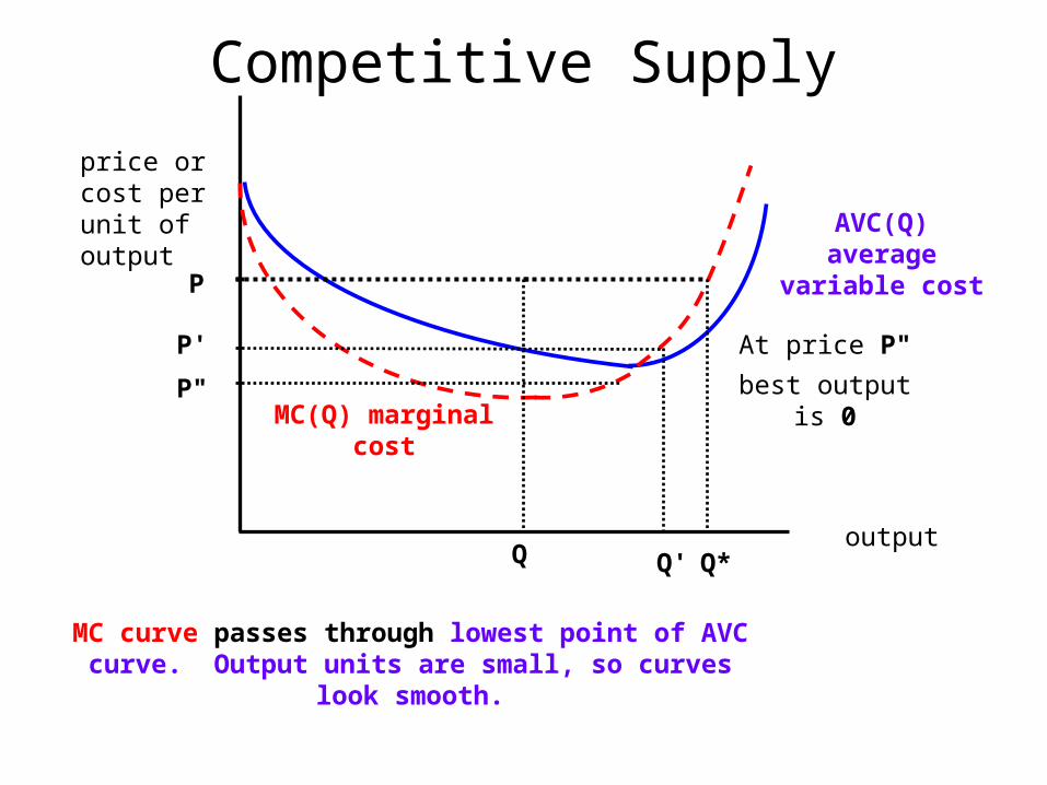
Competitive Supply
output
price or cost per unit of output AVC(Q) average
variable cost
MC(Q) marginal cost
MC curve passes through lowest point of AVC curve. Output units are small, so curves look smooth.
P
Q
At price P"
best output is 0
P"<minimum of AVC
Q*
P'
Q'
P"

Competitive Supply
output
price or cost per unit of output AVC(Q) average
variable cost
MC(Q) marginal cost
MC curve passes through lowest point of AVC curve. Output units are small, so curves look smooth.
P
Q
At price P"
best output is 0
P"<minimum of AVC
Q*
P'
Q'
P"

Competitive Supply
output
price or cost per unit of output AVC(Q) average
variable cost
MC(Q) marginal cost
MC curve passes through lowest point of AVC curve. Output units are small, so curves look smooth.
P
Q
Supply curve: part of MC curve,
part of vertical axis. Supply = 0 at price < min AVC
Q*
P'
Q'
P"min AVC
Competitive Supply
output
price or cost per unit of output AVC(Q) average
variable cost
MC(Q) marginal cost
MC curve passes through lowest point of AVC curve. Output units are small, so curves look smooth.
P
Q
Supply curve: part of MC curve,
part of vertical axis. Supply = 0 at price < min AVC
Q*
P'
Q'
min AVC
Competitive Supply
output
price or cost per unit of output AVC(Q) average
variable cost
MC(Q) marginal cost
MC curve passes through lowest point of AVC curve. Output units are small, so curves look smooth.
P
Q
Supply curve is broken. Output levels 0< Q <Q" never chosen.
P'min AVC
Q"
Competitive Supply
output
price or cost per unit of output AVC(Q) average
variable cost
MC(Q) marginal cost
MC curve passes through lowest point of AVC curve. Output units are small, so curves look smooth.
P
Q
With demand curve like this,
there is no equilibrium price equating supply
and demand.
P'min AVC
Q"
Increasing Returns and Benefits of Markets
In competitive eq, firms cannot have increasing returns where they operate. If they have increasing returns where they operate, they could make more profit by moving in the direction of the increasing returns. They are not maximizing profit at current prices.
The fundamental welfare theorems do not apply.
But markets still contribute to efficiency even if full efficiency is not attained:
Markets allow firms to reach more customers and take advantage of increasing returns. Fewer firms survive, but their average costs are lower.
Competitive Supply
output
price or cost per unit of output AVC(Q) average
variable cost
MC(Q) marginal cost
MC curve passes through lowest point of AVC curve. Output units are small, so curves look smooth.
P
Q
Problem: competitive firm never produces
where AVC is decreasing.
Q*
P'
Q'
min AVC
Producer Surplus
output
price or cost per unit of output AVC(Q) average
variable cost
MC(Q) marginal cost
MC curve passes through lowest point of AVC curve. Output units are small, so curves look smooth.
P
Q
At price P, variable profit = producer surplus = area to
left of supply curve below P
Q*
P
Q'
min AVC
Producer Surplus
output
price or cost per unit of output AVC(Q) average
variable cost
MC(Q) marginal cost
MC curve passes through lowest point of AVC curve. Output units are small, so curves look smooth.
P
Q
At P and Q*, variable profit = PQ*─ VC(Q*) =
area of rectangle to left of Q*
above min AVC, below P
Q*
P
Q'
min AVC
Q*
Producer Surplus
output
price or cost per unit of output AVC(Q) average
variable cost
MC(Q) marginal cost
MC curve passes through lowest point of AVC curve. Output units are small, so curves look smooth.
P
Q
Raising output above Q* raises
variable profit by solid line: P─ MC
Q*
P
Q'
min AVC
Q*
Producer Surplus
output
price or cost per unit of output AVC(Q) average
variable cost
MC(Q) marginal cost
MC curve passes through lowest point of AVC curve. Output units are small, so curves look smooth.
P
Q
Keep raising output above Q* get more solid
lines of variable profit.
Q*
P
Q'
min AVC
Q*
Producer Surplus
output
price or cost per unit of output
MC(Q) marginal cost
MC curve passes through lowest point of AVC curve. Output units are small, so curves look smooth.
P
Q
At price P, and output Q,
variable profit = area to left of supply curve
below P = producer surplus
Q*
P
Q'
min AVC
Consumer Surplus
output
price or cost per unit of output AVC(Q) average
variable cost
MC curve passes through lowest point of AVC curve. Output units are small, so curves look smooth.
Q
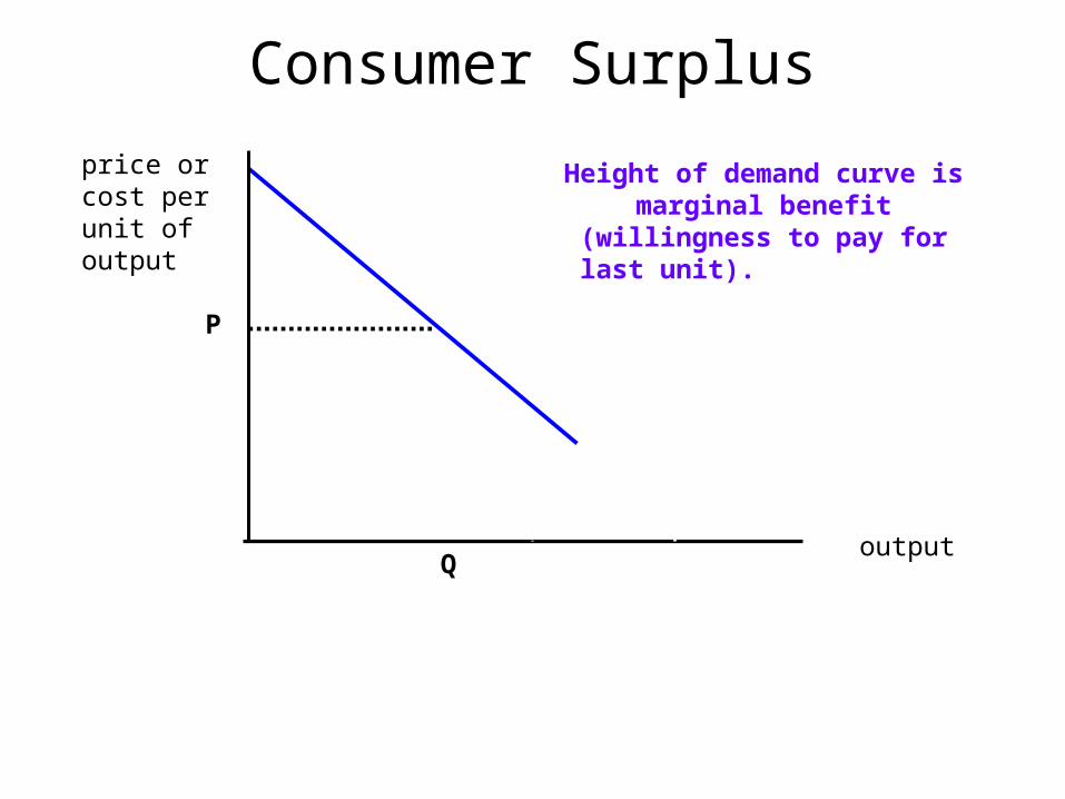
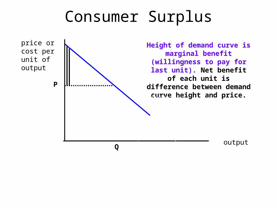
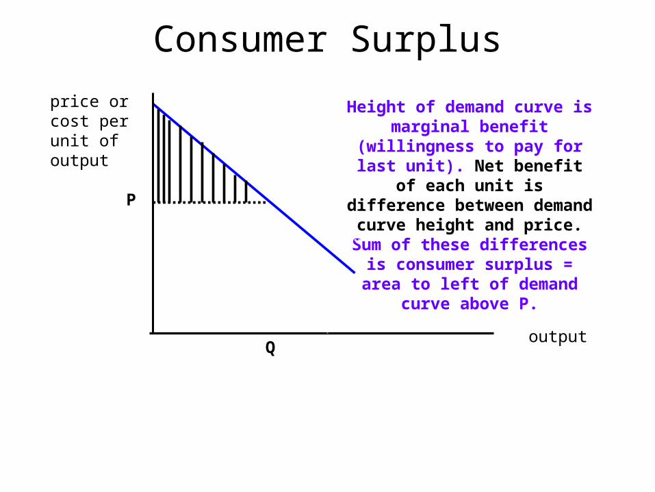
Height of demand curve is marginal benefit (willingness to pay for last unit). Net benefit of each unit is difference between demand curve height and price P. Sum of these differences is
consumer surplus = area to left of demand curve above P.
P'P
Consumer Surplus
output
price or cost per unit of output AVC(Q) average
variable cost
MC curve passes through lowest point of AVC curve. Output units are small, so curves look smooth.
Q
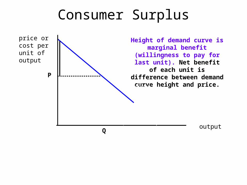
Height of demand curve is marginal benefit (willingness to pay for last unit). Net benefit of each unit is difference between demand curve height and price.
Sum of these differences is consumer surplus = area to left
of demand curve above P.
P'P
Consumer Surplus
output
price or cost per unit of output AVC(Q) average
variable cost
MC curve passes through lowest point of AVC curve. Output units are small, so curves look smooth.
Q
Height of demand curve is marginal benefit (willingness to pay for last unit). Net benefit of each unit is difference between demand curve height and price.
Sum of these differences is consumer surplus = area to left
of demand curve above P.
P'P
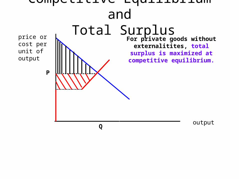
Competitive Equilibrium and Total Surplus
output
price or cost per unit of output AVC(Q) average
variable cost
MC curve passes through lowest point of AVC curve. Output units are small, so curves look smooth.
Q
For private goods without externalitites, total surplus is
maximized at competitive equilibrium.
P'P
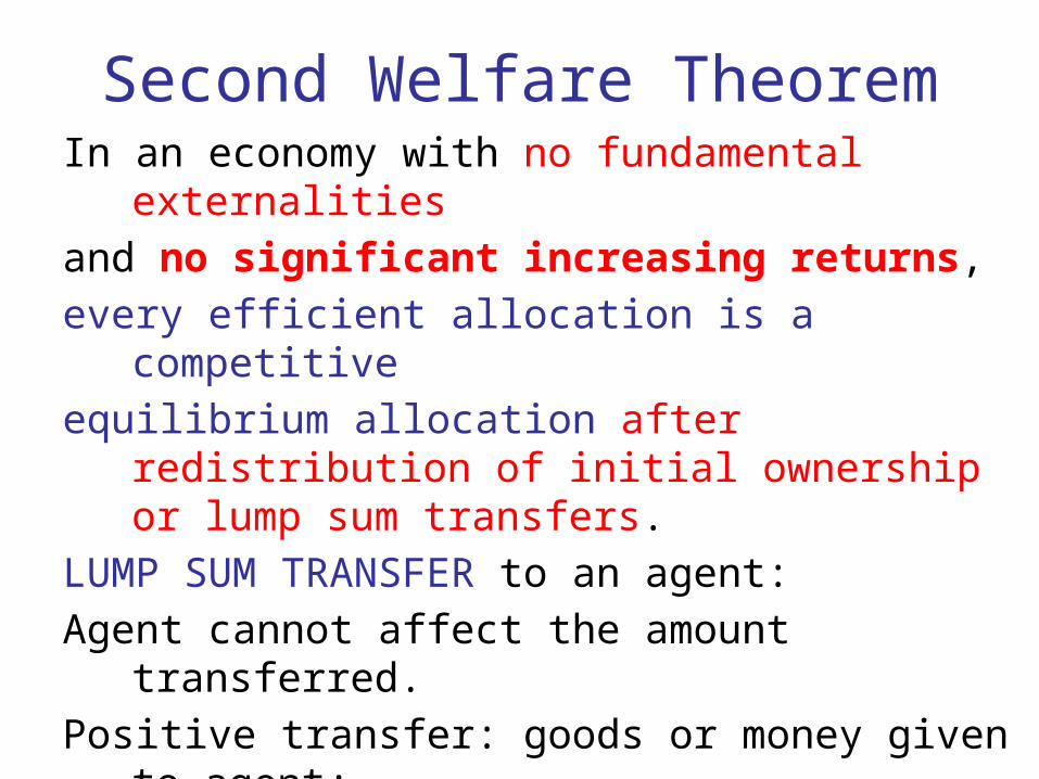
Second Welfare TheoremIn an economy with no fundamental externalities
and no significant increasing returns,
every efficient allocation is a competitive
equilibrium allocation after redistribution of initial ownership or lump sum transfers.
LUMP SUM TRANSFER to an agent:
Agent cannot affect the amount transferred.
Positive transfer: goods or money given to agent;
Negative transfer: goods or money taken away
Negative lump sum transfer = lump sum tax
In Theorem: No bias. Efficient is eq with transfers.

Second Welfare TheoremIn an economy with no fundamental externalities
and no significant increasing returns,
every efficient allocation is a competitive
equilibrium allocation after redistribution of initial ownership or lump sum transfers.
LUMP SUM TRANSFER or TAX leaves prices same for all agents, so MRS can be equal for all.
Other transfers or taxes are distortionary: depend on how much is traded, make buyers and sellers face different prices (example: payroll tax used to pay social security benefits).
Second Welfare TheoremIn an economy with no fundamental externalities
and no significant increasing returns,
every efficient allocation is a competitive
equilibrium allocation after redistribution of initial ownership or lump sum transfers.
LUMP SUM TRANSFER (positive or negative):
Agent cannot affect the amount.
In Theorem: No bias. Under assumptions, every efficient allocation is equilibrium with transfers.

With significant increasing returns, and
decentralized information
(only consumers know their preferences;
only firms know their production possibilities)
NO ALLOCATION MECHANISM ASSURES
PARETO EFFICIENT ALLOCATION.
Calsamiglia, Hurwicz (1975)
Summary: Free Markets and EfficiencyPareto efficiency; Fundamental externality.
Without fundamental externalities, efficiency requires traders to have equal rates of substitution for each pair of divisible goods.
In CE, these rates of substitution are equated.
Conclusion: With small fundamental externalities, competition reaching eq yields nearly efficient allocation. Problems: missing or limited markets; competitive behavior impossible with significant increasing returns; eq may never be reached.
Summary: Free Markets and EfficiencyPareto efficiency; Fundamental externality.
Without fundamental externalities, efficiency requires traders to have equal rates of substitution for each pair of divisible goods.
In CE, these rates of substitution are equated.
Conclusion: With small fundamental externalities, competition reaching eq yields nearly efficient allocation. Problems: With big fundamental externalities, equal private rates of substitution are inefficient.
Summary: Free Markets and EfficiencyPareto efficiency; Fundamental externality.
Without fundamental externalities, efficiency requires traders to have equal rates of substitution for each pair of divisible goods.
In CE, these rates of substitution are equated.
Potential gov roles: promoting markets, making up for missing or limited ones, regulating externalities, promoting competition where inefficient externalities are small.
Summary: Free Markets and EfficiencyPareto efficiency; Fundamental externality.
Without fundamental externalities, efficiency requires traders to have equal rates of substitution for each pair of divisible goods.
In CE, these rates of substitution are equated.
Markets sometimes contribute to efficiency where fundamental welfare theorems do not apply: allow taking advantage of increasing returns.