consumer sentiment and spending on durable goods · aspect of consumer durables, and not their...

FREDERIC S. MISHKIN

University of Chicago

Consumer Sentiment

and Spending

on Durable Goods

MANY studies have found the Index of Consumer Sentiment compiled by the University of Michigan's Survey Research Center to be a useful explanatory variable for consumer expenditure, especially on consumer durables.' Why should this be so? This paper seeks to provide an answer to this question.2

Note: This paper was written for the most part while I was at the Board of Gov- ernors of the Federal Reserve System. I thank Dennis W. Carlton, Nicholas A. Kiefer, George R. Neumann, Susan W. Burch, the staff of the National Income Sec- tion, and members of the Brookings panel for their helpful comments. I also bene- fited from Elizabeth Li's research assistance and from the discussion at seminars given at the Federal Reserve Board and the Econometrics Workshop of the Uni- versity of Chicago. The views expressed here are solely those of the author and do not indicate concurrence by the Federal Reserve System.

1. For example, Eva Mueller, "Ten Years of Consumer Attitude Surveys: Their Forecasting Record," Journal of the American Statistical Association, vol. 58 (De- cember 1963), pp. 899-917; Saul H. Hymans, "Consumer Durable Spending: Ex- planation and Prediction," BPEA, 2:1970, pp. 173-99; F. Thomas Juster and Paul Wachtel, "Inflation and the Consumer," BPEA, 1:1972, pp. 71-114; F. Thomas Juster and Paul Wachtel, "Anticipatory and Objective Models of Durable Goods Demand," American Economic Review, vol. 62 (September 1972), pp. 564-79.

2. Economists at the Survey Research Center have argued that consumer sentiment should be especially critical to decisions to purchase consumer durables because these items are "discretionary"--that is, their purchase can easily be post- poned. See George Katona, The Powerful Consumer: Psychological Studies of the American Economy (McGraw-Hill, 1960), and Mueller, "Ten Years," for examples. One problem with this viewpoint is the difficulty of defining rigorously the degree of an item's postponability.

0007-2303/78/0001-0217$00.25/0 e Brookings Institultion

218 Brookings Papers on Economic Activity, 1:1978

Consumer Sentiment and Liquidity Considerations

Previous work on the liquidity hypothesis emphasizes that the illiquid nature of consumer durables has important effects on spending for such assets.3 This illiquidity means that the consumer incurs some loss when he tries to sell these assets (or borrow against them) to raise cash, especially in an emergency. A consumer suffering financial distress, and un- able to pay his bills readily, would prefer holding highly liquid financial assets. This implies that as the consumer perceives an increasing probability of financial distress, he will decrease his demand for consumer durables and limit his purchases.

One possible interpretation of the index of consumer sentiment is that it actually measures consumers' perceptions of the probability of financial distress. This interpretation appears consistent with the types of questions asked of the survey respondents, which stress personal financial attitudes, expectations about business conditions, and buying conditions for large household goods (a listing of these questions appears in the appendix below). It is also consistent with the view stressed by Juster and Wachtel that the index reflects uncertainty,4 for as the degree of uncertainty in- creases, perceptions of the probability of financial distress would increase also.5

If the index of consumer sentiment reflects perceptions of the probability of financial distress, its crucial relation to consumer durable expenditure becomes clear. A decline in the index would suggest that consumers have perceived a rise in the likelihood of financial distress. They would prefer holding liquid financial assets rather than illiquid consumer durables, and will thus restrict their purchases of durables. The illiquid aspect of consumer durables, and not their discretionary nature, is the reason for the major effects of consumer sentiment.

3. Frederic S. Mishkin, "Illiquidity, Consumer Durable Expenditure, and Mone- tary Policy," American Economic Review, vol. 66 (September 1976), pp. 642-54; and Mishkin, "What Depressed the Consumer? The Household Balance Sheet and the 1973-75 Recession," BPEA, 1:1977, pp. 123-64.

4. F. Thomas Juster and Paul Wachtel, "Uncertainty, Expectations, and Durable Goods Demand Models," in Burkhard Strumpel, James N. Morgan, and Ernest Zahn, eds., Human Behavior in Economic Aflairs: Essays in Honor of George Katona (Jossey-Bass, 1972), pp. 321-45.

5. Mishkin, "Illiquidity," demonstrates this point.

Frederic S. Mishkin 219

The liquidity hypothesis views the composition of the household balance sheet as a major determinant of the probability of financial distress. When indebtedness is high and consumers thus have large con- tractual payments to service it, financial distress is more likely. On the other hand, when the value of financial assets is high, the likelihood of financial distress will fall, since consumers have a larger buffer against bad times. This reasoning suggests that if the index of consumer sentiment is a measure of perceptions of the probability of financial distress, it should be negatively correlated with household indebtedness and positively correlated with the value of financial assets.6

Using data from the period 1954:1 to 1976:4,7 a regression based on ordinary least squares was used to test the proposition above. The index of consumer sentiment was regressed on both household liabilities (DEBT) and financial-asset holdings (FIN). Both the DEBT and FIN variables, which are described in more detail in my previous BPEA paper, are in per capita terms (thousands of 1972 dollars per capita) and are values for the beginning of the quarter. Because of severe autocorrelation of the residuals, the regression has been estimated with a correction for first-order serial correlation using the Cochrane-Orcutt procedure. The resulting estimates, with t statistics in parentheses and the coefficient on u-l equaling the first-order serial-correlation coefficient, appear below.

(1) ICS = 74.57- 38.15 DEBT + 11.55 FIN + 0.7732u_1. (8.57) (-6.96) (6.27)

R2 = 0.8778; Durbin-Watson = 2.20; standard error = 3.57.

The results are consistent with the proposition that ICS measures perceptions of the probability of financial distress and to a great extent reflects shifts in household balance sheets. Both the DEBT and FIN coefficients have the expected signs and are significantly different from zero

6. The index of consumer sentiment is not a measure of consumer welfare. In- creasing indebtedness, for example, may cause a worsening of consumer sentiment if holdings of financial assets did not increase as expected, yet may have enhanced welfare because it supported current expenditure.

7. Before 1962 the ICS survey, which was usually conducted in the middle month or months of a quarter, was taken only sporadically. For the ICS data before 1962, I have used the series found in F. Thomas Juster and Paul Wachtel, "Anticipatory and Objective Models of Durable Goods Demand," Explorations in Economic Research, vol. 1 (Fall 1974), table A-2, which interpolates the data linearly.

S)0

0

C30

0

-O; -~~~~~~~~~~~~~~~~~~~~~~~~~~~~~~~~~~~~~~~~~~~~~~~~~~~~~~~~~~~~~~~~~~~~~1 00 ~cf

PC 00~~~~~~~~~~~O 00. -

(ON 0

0~~~~~~~~~~~~~~~~~~~~~~~

0

'4Z~~~~~~~~~~~~~~~~~~~

ON u

~~~~ 0 ON 00 0~~~~~~~~~~~~~~~~~~~~~~0' 0

0


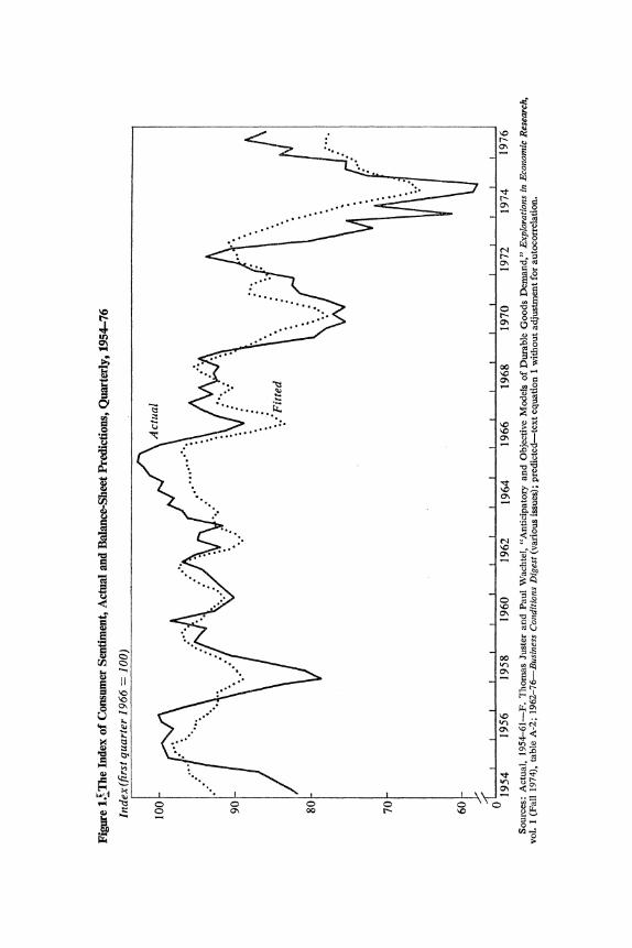
at the 1 percent level (with t statistics exceeding 6 in absolute value).,8 The within-sample tracking of equation 1 when there is no adjustment for autocorrelation, as shown in figure 1, indicates that balance-sheet movements alone can account for the overall cycles in consumer sentiment, explaining 70 percent of the variance in ICS. With the autocorrelation adjustment, equation 1 explains 88 percent of the variance of ICS.

The liquidity hypothesis also implies that income expectations, as to both the mean and the variance, affect consumer perceptions of the probability of financial distress.9 Higher expected income lowers the probability of distress and greater uncertainty raises it. In addition, Hymans, as well as Juster and Wachtel,'0 points to the effects of price inflation on consumer sentiment. To reflect these factors, income and price variables similar to those used by Hymans have been added to the regression equation 1.11 Also a dummy variable for the oil embargo period has been added, since income, price, and balance-sheet variables would not capture changes in consumer expectations due to an adverse, exogenous, economic event.'2 The ordinary least-squares estimates of this regression, estimated over the period 1954:1 to 1976:4, again correcting for serial correlation, appear below. Note that although many of the explanatory variables are determined simultaneously with ICS, since consumer senti-

8. Some of the possible effects of aggregation on the size of the DEBT and FIN coefficients have been discussed in Mishkin, "What Depressed the Consumer?"

The opposite signs on these coefficients could result from an attempt to track the essentially trendless ICS with those variables, both of which have strong upward trends. Adding a time-trend variable (which turns out to be very insignificant) to equation 1 or deflating the DEBT and FIN variables by income to eliminate trend does not appreciably alter the results. The DEBT and FIN coefficients retain their signs and high level of statistical significance.

The null hypothesis that the DEBT and FIN coefficients are equal but opposite in sign can be rejected at the 1 percent level: t = 6.55 while the critical t at 1 percent is 2.6.

9. See the more formal model contained in Mishkin, "Illiquidity." 10. Hymans, "Consumer Durable Spending," pp. 174-77, and Juster and Wach-

tel, "Inflation and the Consumer," pp. 96-98. 11. Instead of the Hymans variables, I also tried the inflation and unemploy-

ment variables used by Michael C. Lovell, "Why Was the Consumer Feeling So Sad?" BPEA, 2:1975, pp. 473-79; qualitatively, the results were not appreciably different although the fit was slightly worse. In particular, the coefficients of the balance-sheet variables remained highly significant and of the appropriate sign.

12. Only the 1974:1 survey was taken during the oil embargo, even though the embargo started in the fourth quarter of 1973.


ment has been found to affect expenditure with a lag13 the regression is part of a recursive system and can be estimated consistently with ordinary least squares.

(2) ICS = 42.20 + 136.10 INCOME - 93.68 PRICE (0.41) (3.26) (- 1.19)

- 11.79 DUM - 26.36 DEBT + 7.35 FIN + 0.7705u_, (-5.09) (-4.08) (3.85)

R2 = 0.9225; Durbin-Watson = 1.87; standard error = 2.89.

where

INCOME= YD/(1/8) E YJiL 0

PRICE = PCON/(1/8) E PCON-i 0

D UM = 1 in 1974:1, 0 otherwise.

In these last expressions

YD = real personal disposable income per capita in thousands of 1972 dollars, from the MPS data bank

PCON = consumption deflator from the MPS data bank.

The additional variables significantly improve the fit of the regression: 14,15 when there is no adjustment for autocorrelation, the percentage of explained variation in ICS rises to 80 percent, and it is 92 percent when there is such an adjustment. The balance-sheet variables continue to be important explanatory variables of ICS.10 The DEBT and FIN coefficients

13. In the works cited in note 1 only the lagged values of ICS have proved to be significantly different from zero in consumer-durable regressions. I also tested for the significance of the current value of ICS in consumer-durable regressions and found it to be insignificant.

14. The hypothesis that these variables have zero coefficients is rejected at the 1 percent level; F(3,86) = 16.6, while the critical F.o1 is approximately 4.

15. I tried lagging these variables as Hymans, "Consumer Durable Spending," p. 177, and Juster and Wachtel, "Inflation and the Consumer," p. 97, at times have done. The t statistics for these variables decline substantially in size and the fit of the equation deteriorates, while the balance-sheet variables become even more significant.

16. The balance-sheet variables do contribute significantly to improving the fit of


are still significant at the 1 percent level with expected signs, and their size is approximately two-thirds of that found in equation 1 17

Equation 2 reveals how much of the most severe postwar cyclical decline in ICS-from the third quarter of 1972 to the first quarter of 1975 -can be attributed to the effects from balance sheets versus those from income and inflation. Of the 36-point drop in ICS, 14.1 points can be explained by balance-sheet movements, while 13.8 points can be attributed to income and inflation.18

As shown in equation 3, the decomposition of the household balance sheet into its debt and financial-asset components is crucial to these significant findings of balance-sheet effects.

(3) ICS -259.09 + 136.55 INCOME - 301.17 PRICE (2.73) (3.00) (-4.50)

-11.66 DUM + 0.07 WEALTH + 0.7860u_l. (-4.66) (0.08)

R2= 0.9073; Durbin-Watson = 1.68; standard error = 3.15.

When a measure of real per capita net worth (WEALTH) replaces the DEBT and FIN variables, its t statistic is an insignificant 0.08.

One additional issue relates to the previous work of Hymans, Juster and Wachtel, and Lovell.'9 Their estimated equations explaining ICS include the ICS lagged one quarter (ICS-1) as an explanatory variable. This variable may reflect a slow response of consumer sentiment to the other explanatory variables, or the slow approach of consumer sentiment to its equilibrium value because consumers "catch" optimism or pessimism

the regression. The hypothesis that both these variables have zero coefficients is rejected at the 1 percent level; F(2,86) = 8.5 and the critical F.01 is approximately 5.

17. Equations 1 and 2 have also been estimated in log-linear form (except for DUM, of course) and the results are not appreciably different. In particular, the t statistics of the DEBT and FIN coefficients change by less than S percent. In the log-linear versioni of equation 2, the absolute value of the DEBT and FIN elastici- ties are not significantly different from each other (t = 1.35), thus indicating that, in this case, the ratio of financial assets to debt could be the relevant explanatory variable for ICS.

18. The remaining 8.1 points are unexplained and appear as changes in the residuals of equation 2.

19. Hymans, "Consumer Durable Spending," p. 177; Juster and Wachtel, "Infla- tion and the Consumer," p. 97; and Lovell, "Why Was the Consumer Feeling So Sad?"


from each other. Thus ICS1 was added to equation 2 to test for these effects with the following results:

(4) ICS = 41.13 + 134.42 INCOME - 94.82 PRICE (0.40) (3.18) (-1.22)

- 12.21 DUM - 24.91 DEBT + 6.96 FIN (-4.91) (-3.66) (3.43)

+0.04 ICS-1 + 0.7505u_l. (0.50)

RI = 0.9227; Durbin-Watson = 1.91; standard error = 2.91.

Inclusion of the lagged dependent variable affects estimated coefficients

of the other right-hand-side variables only marginally, with the DEBT, FIN, INCOME, and DUM coefficients still retaining their high statistical

significance. Moreover, the estimated coefficient of ICS1 is only 0.04 and

its t statistic 0.5, indicating an absence of the lag effects found by Hymans,

Juster and Wachtel, and Lovell. Their significant positive coefficients on ICS1 probably stem from their failure to correct for possible serial corre-

lation. If there is uncorrected serial correlation of the residuals, inclusion

of the lagged dependent variable leads to biased coefficients as well as to a

biased Durbin-Watson statistic. Positive autocorrelation, as is found in

equations 1 and 2, will usually lead to a spurious positive coefficient on

the lagged dependent variable because this variable tries to capture the

correction for serial correlation. The empirical evidence presented here is consistent with the view that

the index of consumer sentiment reflects in large part consumers' percep-

tions of the likelihood of financial distress and is considerably affected by shifts in the composition of the balance sheets of American households.20

The Usefulness of Consumer Sentiment Measures

Several studies have found some measure of consumer sentiment to be

a useful addition to a standard stock-adjustment model of demand for

20. Included in the financial-assets variable is the value of common stocks. Be- cause consumer perceptions of uncertainty and changes in income expectations affect stock-market valuations, the large impact of the FIN variable on durable expenditure might reflect balance-sheet effects only in part. Unfortunately, the time- series data used here cannot help sort out how much of the FIN coefficient repre- sents expectation effects and how much balance-sheet effects.


consumer durables.2' Consumer-durable expenditure and the index of consumer sentiment have displayed great volatility in the last few years, thus providing data for more powerful tests of the importance of consumer sentiment to durable expenditures. Do the additional quarterly data from the last few years and the major revision by the Commerce Department of the national income accounts support the predictive ability of consumer sentiment measures? Table 1 presents estimates of a non- balance-sheet stock-adjustment model used in my earlier paper22 to which several sentiment variables commonly used in other studies are added as explanatory variables: these include ICS, the change in ICS, and a filtered version of ICS (FICS) developed by Juster and Wachtel23-all of which are lagged one quarter. All equations in table 1 and those that follow are estimated with instrumental variables with a correction for first-order serial correlation to produce consistent estimates, free of simultaneous- equation bias.24 The estimation sample period runs from 1954:1 to 1976:4 with six quarters excluded because of auto strikes.25 The results do indicate the usefulness of consumer sentiment variables in consumer-durable models, with the level of ICS faring best, as in regression 1-1 where the asymptotic t statistic of its coefficient exceeds 4. This coefficient implies that a one-point change in ICS leads to a short-run change of $0.3 billion (1972 value) in consumer-durable expenditure. In contrast with the

21. Again, see the work cited in note 1. 22. Mishkin, "What Depressed the Consumer?" 23. Juster and Wachtel, "Uncertainty." 24. The list of instruments includes exports, the discount rate, unborrowed re-

serves plus currency outside of banks, federal government expenditures, the tax rate on personal income, these five variables lagged one period, the constant term, and population. Because there is a correction for serial correlation, the KCD1, DEBT, and lagged sentiment variables should be taken as predetermined in the regressions in which they appear and are thus used as instruments. All other variables are treated as endogenous and are thus instrumental in the estimation procedure. The FIN variable is not treated as predetermined because the average of the current and lagged values of stocks is used in computing its value. Note that in my previous estimates of consumer-durable equations I did not treat the DEBT and KCD1 variables as predetermined, as would be appropriate. The results are not appreciably different if these variables are not treated as predetermined. The estimation method developed by Ray C. Fair, "The Estimation of Simultaneous Equation Models with Lagged Endogenous Variables and First Order Serially Correlated Errors," Econo- metrica, vol. 38 (May 1970), pp. 507-16, has been used here with the appropriate additional instruments.

25. The quarters excluded are 1964:4 to 1965:2 and 1970:4 to 1971:2.


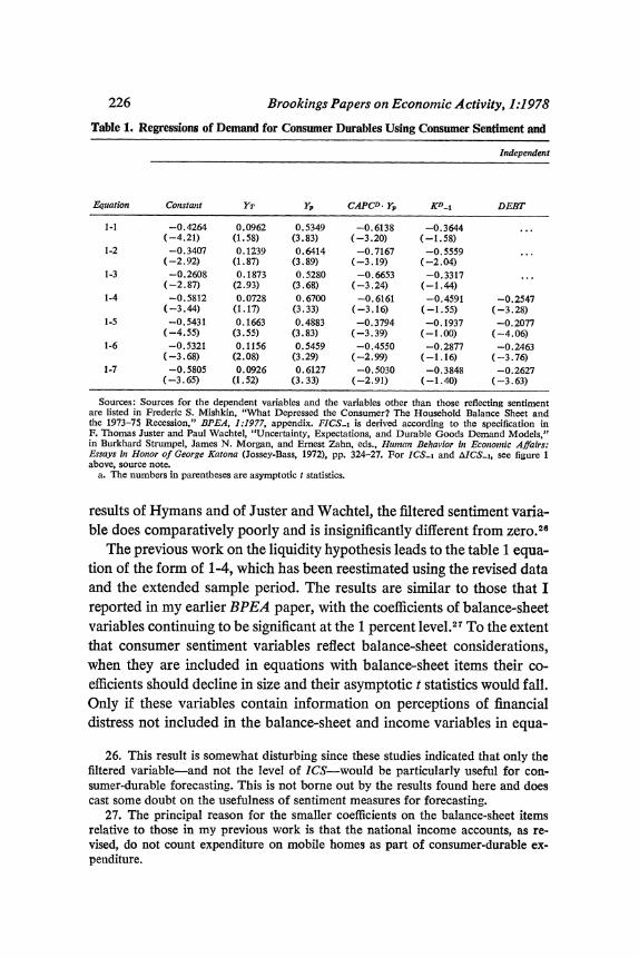
Table 1. Regressions of Demand for Consumer Durables Using Consumer Sentiment and

Independent

Equation Constant YT YP CAPCD. YP KD_i DEBT

1-1 -0.4264 0.0962 0.5349 -0.6138 -0.3644 ... (-4.21) (1.58) (3.83) (-3.20) (-1.58)

1-2 -0.3407 0.1239 0.6414 -0.7167 -0.5559 (-2.92) (1.87) (3.89) (-3.19) (-2.04)

1-3 -0.2608 0.1873 0.5280 -0.6653 -0.3317 ... (-2.87) (2.93) (3.68) (-3.24) (-1.44)

1-4 -0.5812 0.0728 0.6700 -0.6161 -0.4591 -0.2547 (-3.44) (1.17) (3.33) (-3.16) (-1.55) (-3.28)

1-5 -0.5431 0.1663 0.4883 -0.3794 -0.1937 -0.2077 (-4.55) (3.55) (3.83) (-3.39) (-1.00) (-4.06)

1-6 -0.5321 0.1156 0.5459 -0.4550 -0.2877 -0.2463 (-3.68) (2.08) (3.29) (-2.99) (-1.16) (-3.76)

1-7 -0.5805 0.0926 0.6127 -0.5030 -0.3848 -0.2627 (-3.65) (1.52) (3.33) (-2.91) (-1.40) (-3.63)

Sources: Sources for the dependent variables and the variables other than those reflecting sentiment are listed in Frederic S. Mishkin, "Vhat Depressed the Consumer? The Household Balance Sheet and the 1973-75 Recession," BPEA, 1:1977, appendix. FICS-1 is derived according to the specification in F. Thomas Juster and Paul Wachtel, "Uncertainty, Expectations, and Durable Goods Demand Models," in Burkhard Strumpel, James N. Morgan, and Ernest Zahn, eds., Human Behavior in Economic Affairs: Essays in Honor of George Katona (Jossey-Bass, 1972), pp. 324-27. For ICS-1 and MICS-1, see figure 1 above, source note.

a. The numbers in parentheses are asymptotic t statistics.

results of Hymans and of Juster and Wachtel, the filtered sentiment variable does comparatively poorly and is insignificantly different from zero.26

The previous work on the liquidity hypothesis leads to the table 1 equation of the form of 1-4, which has been reestimated using the revised data and the extended sample period. The results are similar to those that I reported in my earlier BPEA paper, with the coefficients of balance-sheet variables continuing to be significant at the 1 percent level.27 To the extent that consumer sentiment variables reflect balance-sheet considerations, when they are included in equations with balance-sheet items their coefficients should decline in size and their asymptotic t statistics would fall. Only if these variables contain information on perceptions of financial distress not included in the balance-sheet and income variables in equa-

26. This result is somewhat disturbing since these studies indicated that only the filtered variable-and not the level of ICS-would be particularly useful for consumer-durable forecasting. This is not borne out by the results found here and does cast some doubt on the usefulness of sentiment measures for forecasting.

27. The principal reason for the smaller coefficients on the balance-sheet items relative to those in my previous work is that the national income accounts, as revised, do not count expenditure on mobile homes as part of consumer-durable expenditure.


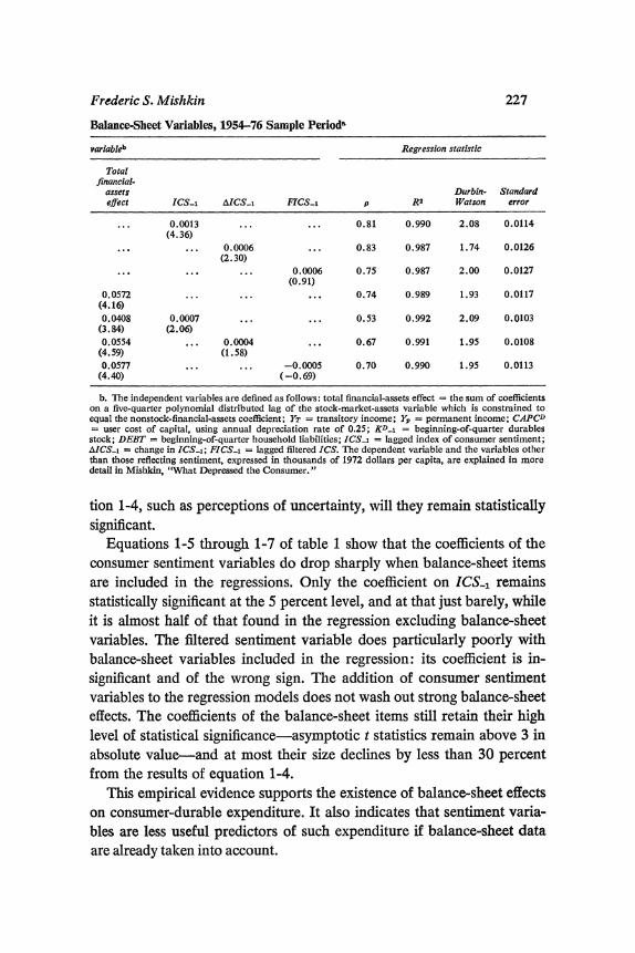
Balance-Sheet Variables, 1954-76 Sample Periods

variableb Regression statistic

Total financial-

assets Durbin- Standard effect ICS_1 AICS.i FICS-i p R2 Watson error

0.0013 ... ... 0.81 0.990 2.08 0.0114 (4.36)

... ... 0.0006 ... 0.83 0.987 1.74 0.0126 (2.30)

... ... ... 0.0006 0.75 0.987 2.00 0.0127 (0.91)

0.0572 ... ... ... 0.74 0.989 1.93 0.0117 (4.16) 0.0408 0.0007 ... ... 0.53 0.992 2.09 0.0103

(3.84) (2.06) 0.0554 ... 0.0004 ... 0.67 0.991 1.95 0.0108

(4.59) (1.58) 0.0577 ... ... -0.0005 0.70 0.990 1.95 0.0113

(4.40) (-0.69)

b. The independent variables are defined as follows: total financial-assets effect the sum of coefficients on a five-quarter polynomial distributed lag of the stock-market-assets variable which is constrained to equal the nonstock-financial-assets coefficient; YT transitory income; Y = permanent income; CAPCD = user cost of capital, using annual depreciation rate of 0.25; kD-i = beginning-of-quarter durables stock; DEBT = beginning-of-quarter household liabilities; ICS-i = lagged index of consumer sentiment; AICS_i = change in ICS1; FICS-1 = lagged filtered ICS. The dependent variable and the variables other than those reflecting sentiment, expressed in thousands of 1972 dollars per capita, are explained in more detail in Mishkin, "What Depressed the Consumer. "

tion 1-4, such as perceptions of uncertainty, will they remain statistically significant.

Equations 1-5 through 1-7 of table 1 show that the coefficients of the consumer sentiment variables do drop sharply when balance-sheet items are included in the regressions. Only the coefficient on ICS 1 remains statistically significant at the 5 percent level, and at that just barely, while it is almost half of that found in the regression excluding balance-sheet variables. The filtered sentiment variable does particularly poorly with balance-sheet variables included in the regression: its coefficient is insignificant and of the wrong sign. The addition of consumer sentiment variables to the regression models does not wash out strong balance-sheet effects. The coefficients of the balance-sheet items still retain their high level of statistical significance-asymptotic t statistics remain above 3 in absolute value-and at most their size declines by less than 30 percent from the results of equation 1-4.

This empirical evidence supports the existence of balance-sheet effects on consumer-durable expenditure. It also indicates that sentiment variables are less useful predictors of such expenditure if balance-sheet data are already taken into account.


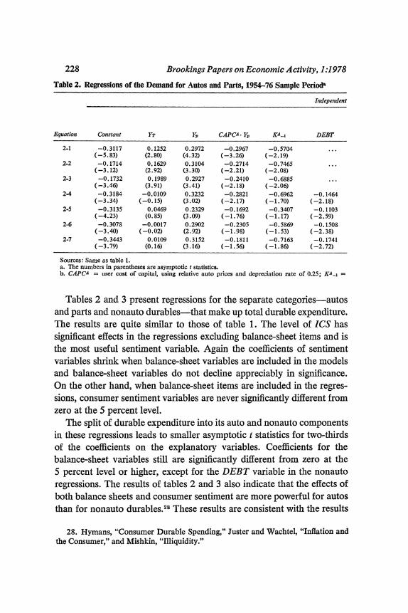
Table 2. Regressions of the Demand for Autos and Parts, 1954-76 Sample Periods

Independent

Equation Constant YT YP CAP CA. YP KA_i DEBT

2-1 -0.3117 0.1252 0.2972 -0.2967 -0.5704 ... (-5.83) (2.80) (4.32) (-3.26) (-2.19)

2-2 -0.1714 0.1629 0.3104 -0.2714 -0.7465 ... (-3.12) (2.92) (3.30) (-2.21) (-2.08)

2-3 -0.1732 0.1989 0.2927 -0.2410 -0.6885 ... (-3.46) (3.91) (3.41) (-2.18) (-2.06)

2-4 -0.3184 -0.0109 0.3232 -0.2821 -0.6962 -0.1464 (-3.34) (-0.15) (3.02) (-2.17) (-1.70) (-2.18)

2-5 -0.3135 0.0469 0.2329 -0.1692 -0.3407 -0.1103 (-4.23) (0.85) (3.09) (-1.76) (-1.17) (-2.59)

2-6 -0.3078 -0.0017 0.2902 -0.2305 -0.5869 -0.1508 (-3.40) (-0.02) (2.92) (-1.98) (-1.53) (-2.38)

2-7 -0.3443 0.0109 0.3152 -0.1811 -0.7163 -0.1741 (-3.79) (0.16) (3.16) (-1.56) (-1.86) (-2.72)

Sources: Same as table 1. a. The numbers in parentheses are asymptotic t statistics. b. CAPCA = user cost of capital, using relative auto prices and depreciation rate of 0.25; KA-i =

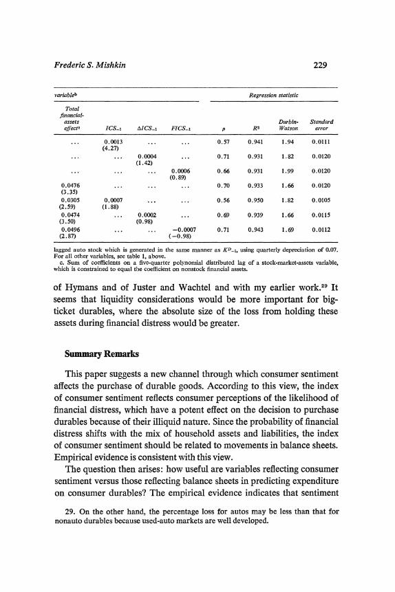
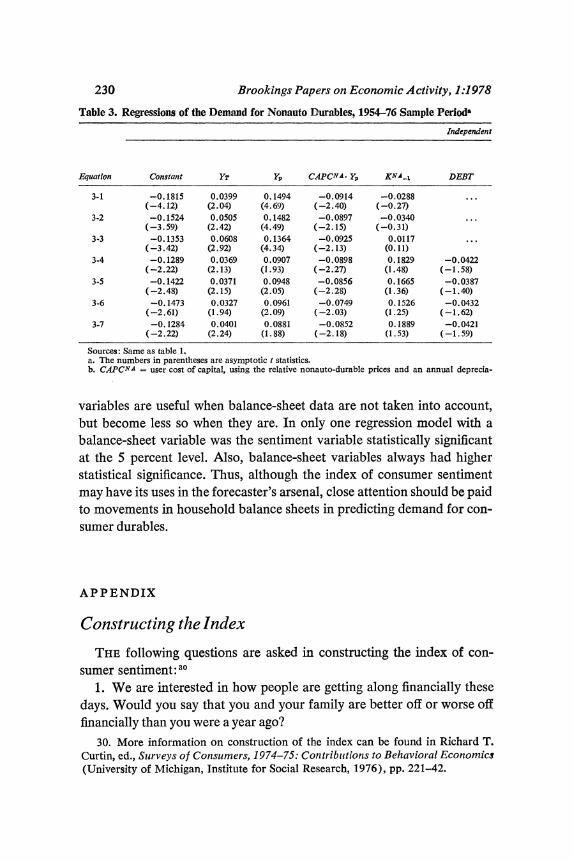
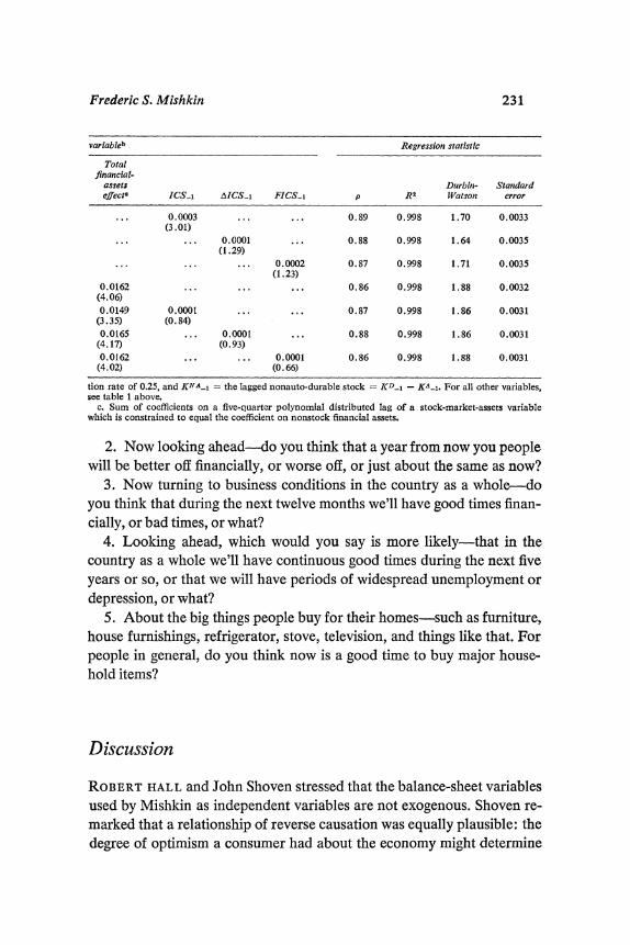
Tables 2 and 3 present regressions for the separate categories-autos and parts and nonauto durables-that make up total durable expenditure. The results are quite similar to those of table 1. The level of ICS has significant effects in the regressions excluding balance-sheet items and is the most useful sentiment variable. Again the coefficients of sentiment variables shrink when balance-sheet variables are included in the models and balance-sheet variables do not decline appreciably in significance. On the other hand, when balance-sheet items are included in the regressions, consumer sentiment variables are never significantly different from zero at the 5 percent level.

The split of durable expenditure into its auto and nonauto components in these regressions leads to smaller asymptotic t statistics for two-thirds of the coefficients on the explanatory variables. Coefficients for the balance-sheet variables still are significantly different from zero at the 5 percent level or higher, except for the DEBT variable in the nonauto regressions. The results of tables 2 and 3 also indicate that the effects of both balance sheets and consumer sentiment are more powerful for autos than for nonauto durables.28 These results are consistent with the results

28. Hymans, "Consumer Durable Spending," Juster and Wachtel, "Inflation and the Consumer," and Mishkin, "Illiquidity."



Total financial-

assets Durbin- Standard effecto ICS_1 AICS_i FICS-1 p R2 Watson error

... 0.0013 ... ... 0.57 0.941 1.94 0.0111 (4.27)

... ... 0.0004 ... 0.71 0.931 1.82 0.0120 (1.42)

... ... ... 0.0006 0.66 0.931 1.99 0.0120 (0.89)

0.0476 ... ... ... 0.70 0.933 1.66 0.0120 (3.35) 0.0305 0.0007 ... ... 0.56 0.950 1.82 0.0105

(2.59) (1.88) 0.0474 ... 0.0002 ... 0.69 0.939 1.66 0.0115

(3.50) (0.98) 0.0496 ... ... -0.0007 0.71 0.943 1.69 0.0112

(2.87) (-0.98)

lagged auto stock which is generated in the same manner as KD-i, using quarterly depreciation of 0.07. For all other variables, see table 1, above.

c. Sum of coefficients on a five-quarter polynomial distributed lag of a stock-market-assets variable, which is constrained to equal the coefficient on nonstock financial assets.

of Hymans and of Juster and Wachtel and with my earlier work.29 It seems that liquidity considerations would be more important for big- ticket durables, where the absolute size of the loss from holding these assets during financial distress would be greater.

Summary Remarks

This paper suggests a new channel through which consumer sentiment affects the purchase of durable goods. According to this view, the index of consumer sentiment reflects consumer perceptions of the likelihood of financial distress, which have a potent effect on the decision to purchase durables because of their illiquid nature. Since the probability of financial distress shifts with the mix of household assets and liabilities, the index of consumer sentiment should be related to movements in balance sheets. Empirical evidence is consistent with this view.

The question then arises: how useful are variables reflecting consumer sentiment versus those reflecting balance sheets in predicting expenditure on consumer durables? The empirical evidence indicates that sentiment

29. On the other hand, the percentage loss for autos may be less than that for nonauto durables because used-auto markets are well developed.


Table 3. Regressions of the Demand for Nonauto Durables, 1954-76 Sample Period&

Independent

Equation Constant YT Y1. CAPCNA. YP KNAi_ DEBT

3-1 -0.1815 0.0399 0.1494 -0.0914 -0.0288 ... (-4.12) (2.04) (4.69) (-2.40) (-0.27)

3-2 -0.1524 0.0505 0.1482 -0.0897 -0.0340 ... (-3.59) (2.42) (4.49) (-2.15) (-0.31)

3-3 -0.1353 0.0608 0.1364 -0.0925 0.0117 ... (-3.42) (2.92) (4.34) (-2.13) (0. 11)

3-4 -0.1289 0.0369 0.0907 -0.0898 0.1829 -0.0422 (-2.22) (2.13) (1.93) (-2.27) (1.48) (-1.58)

3-5 -0.1422 0.0371 0.0948 -0.0856 0.1665 -0.0387 (-2.48) (2.15) (2.05) (-2.28) (1.36) (-1.40)

3-6 -0. 1473 0.0327 0.0961 -0.0749 0.1526 -0.0432 (-2.61) (1.94) (2.09) (-2.03) (1.25) (-1.62)

3-7 -0.1284 0.0401 0.0881 -0.0852 0.1889 -0.0421 (-2.22) (2.24) (1.88) (-2.18) (1.53) (-1.59)

Sources: Same as table 1. a. The numbers in parentheses are asymptotic t statistics. b. CAPCNA = user cost of capital, using the relative nonauto-durable prices and an annual deprecia-

variables are useful when balance-sheet data are not taken into account, but become less so when they are. In only one regression model with a balance-sheet variable was the sentiment variable statistically significant at the 5 percent level. Also, balance-sheet variables always had higher statistical significance. Thus, although the index of consumer sentiment may have its uses in the forecaster's arsenal, close attention should be paid to movements in household balance sheets in predicting demand for consumer durables.

APPENDIX

Constructing the Index

THE following questions are asked in constructing the index of consumer sentiment:30

1. We are interested in how people are getting along financially these days. Would you say that you and your family are better off or worse off financially than you were a year ago?

30. More information on construction of the index can be found in Richard T. Curtin, ed., Surveys of Consumers, 1974-75: Contribuitions to Behavior al Economics (University of Michigan, Institute for Social Research, 1976), pp. 221-42.



Total financial-

assets Durbin- Standard effecto ICS_1 tICSi FICS-i p R2 Watson error

... 0.0003 ... ... 0.89 0.998 1.70 0.0033 (3.01)

... ... 0.0001 ... 0.88 0.998 1.64 0.0035 (1.29)

... ... ... 0.0002 0.87 0.998 1.71 0.0035 (1.23)

0.0162 ... ... ... 0.86 0.998 1.88 0.0032 (4.06) 0.0149 0.0001 ... ... 0.87 0.998 1.86 0.0031

(3.35) (0.84) 0.0165 ... 0.0001 ... 0.88 0.998 1.86 0.0031

(4.17) (0.93) 0.0162 ... ... 0.0001 0.86 0.998 1.88 0.0031

(4.02) (0.66)

tion rate of 0.25, and KNA_1 = the lagged nonauto-durable stock = KD_1 - KA-1. For all other variables, see table 1 above.

c. Sum of coefficients on a five-quarter polynomial distributed lag of a stock-market-assets variable which is constrained to equal the coefficient on nonstock financial assets.

2. Now looking ahead-do you think that a year from now you people will be better off financially, or worse off, or just about the same as now?

3. Now turning to business conditions in the country as a whole-do you think that during the next twelve months we'll have good times financially, or bad times, or what?

4. Looking ahead, which would you say is more likely-that in the country as a whole we'll have continuous good times during the next five years or so, or that we will have periods of widespread unemployment or depression, or what?

5. About the big things people buy for their homes-such as furniture, house furnishings, refrigerator, stove, television, and things like that. For people in general, do you think now is a good time to buy major household items?

Discussion

ROBERT HALL and John Shoven stressed that the balance-sheet variables used by Mishkin as independent variables are not exogenous. Shoven remarked that a relationship of reverse causation was equally plausible: the degree of optimism a consumer had about the economy might determine


the composition of his portfolio. Hall saw no evidence of a causal relationship in which fear of financial distress aroused by the balance-sheet variables led to a decline in consumer sentiment. And in view of the high degree of concentration of equity ownership in the United States, the coefficient on the assets variable was much too high to be interpreted as a wealth effect. He felt that Mishkin's analysis showed only that consumer sentiment, consumer spending, and the stock market seem to be affected by common factors and are therefore highly correlated. Mishkin replied that the importance of household liabilities in his analysis provided some support for the view that changes in balance sheets affect consumer sentiment and consumer spending. Also, as was mentioned in the discussion of his previous BPEA paper, there is evidence that is not susceptible to the reverse-causation problem in Friend and Lieberman's cross-section study, and that indicates that the stock market can have sizable effects on consumer spending.

Thomas Juster believed there were strong reasons to expect some relationship between financial variables and consumer sentiment, but Mish- kin's was the first study to have found them. He suggested that the inclusion of the most recent three years had led to this finding. Frank Schiff reasoned that the effects on sentiment might occur only beyond certain threshold levels of indebtedness or rate of change in stock-market values. He also urged a fuller exploration of the possibilities for greater use of direct observation of such effects through interview surveys.

Juster found it implausible that, with no change in net worth, consumers would feel worse off simply by changing one asset for another, a result implied by Mishkin's equations. Why would someone feel more gloomy after buying a car? Shoven remarked that one might expect the opposite result: more confident people were more prepared to go into debt. Michael Lovell noted that these considerations raised the issue of whether wealth or liquid assets belonged in explanations of consumer behavior. Mishkin replied that the analysis of this paper is quite consistent with the increased willingness of more confident people to incur debt: a healthy balance-sheet position at the beginning of the period, which en- courages confidence, will make the consumer more likely to purchase durables and incur debt. In addition, the purchase of durables is often accom- panied by continuing improvements in the consumer's financial position, and thus the consumer would not necessarily feel more gloomy after a purchase of durables.

consumer sentiment and spending on durable goods · aspect of consumer durables, and not their...

Documents