Lw

R68-51

CONSUMER PREFERENCES ANDQ0 THE ABSTRACT MODE MODEL:

S BOSTON METROPOLITAN AREA

by

"Rodney Poul Ploordo

MAJuS. 1968

Cabide Mascuet 02139

C L f A Qi N ýj U j•,rA u.I ,[

f.al

Research Report R68-51

CONSUMER PREFERENCES ANDTHE ABSTRACT MODE MODEL:BOSTON METROPOLITAN AREA

by

Rodney Paul Plourde

SEARCH AND CHOICE IN TRANSPORT SYSTEMS PLANNING

Volume XII of a Series

Prepared in cooperation with theM.I.To Urban Systems Laboratory

Sponsored by the U.S. Department ofTransportation, the General Motors Grant

for Highway Transportation Research

Transportation Systems DivisionDepartment of Civil Engineering

Massachusetts Institute of TechnologyCambridge, Massachusetts 02139

June, 1968

ACKNOWLEDGEMENtS

This report is part of a series in a program of research into the

process of transpcrt Pvstems planning. The basic support for this research

was provided by the U.S. Department of Transportation, Office of Systems

Analysis, through contiact 7-351 40 (DSR 70386). Additional support for

portions of this research was provided by the General Motors Grant for Highway

Transportation Research (DSR 70065); by the Ford Foundation through a grant

to the Urban Systems Laboratory of M.I.T. and by the National Science Founda-

tion through a fellowship to the author. The support of these agencies is

gratefully acknowledged-

Clearly, however, the opinions expressed herein are those of the

individual authors and do not necessarily represent the views of any research

sponsor.

The need for fundamental, exploratory research in the overall area was

initially recognized by A. Scheffer Lang, then Deputy Undersecretary of

Commerce for Transportation Research, and Henry W. Bruck, then Director,

Transport Systems Planning livision, Office of High Speed Ground Transportation.

Their interest and support stimulated the initiation of this project. The

guidance and interest of Dr. Edward Golding of the Office of Systems Analysis,

Department of Transportation, is also gratefully acknowledged. Dr. Golding

in particular encouraged us to show the relevance of this research to

transportation policy through the "prototype analysis".

Appreciation is also expressed to Professor Joseph I. Stafford for his

supervision of the work covered in this report; to Thcmas N. Harvey for his

assistance in securing the necessary data; and to Bernard Andre Genest and

the M I.T. Computations Center consultants for their assistance in processing

the data

TABLE OF CONTENTSPage

INTRODUCTION 1

CHAPTER ONE

MODEL DEFINITION AND DELINEATIONOF STUDY AREA

1.1 Why the Abstract Mode Model 2

1.2 The Abstract Mode Model - Definition 5

1.3 Study Area - Metropolitan Boston 8

1.4 Input Parameters to the Model 12

CHAPTER TWO

THE TRADEOFF RATIO CONCEPT

2.1 The Tradeoff Ratio - Background and Definition 15

2.9 Derivation of the Tradeoff Ratios from an Abstract 17

Mode Formulation

2.3 The Tradeoff Ratio - Implications for Transport 24Planning and Design

CHAPTER THREE

MODEL EVALUATION

3.1 The Abstract Mode Model, Good or Bad? - Summary 25

3.2 Statistical Evaluation - Conclusions 26

3 3 Strengths and Weaknesses of the Model 38

j.4 Model Results Plus Tradeoff Ratios - Design Implications 40

Su,1MARY AND CONCLUSIONS 43

BIBLIOGRAPHY 45

APPENDIX - LIST OF FIGURES AND TABLES 48

1

INTRODUCTION

Travel demand models predict the number of people who will freely

choose to use a given system at a specified level of service. Use is

one measure of the "goodness" or effectiveness of a system, and is the

end product of many individual consumer trip decisions.

A travel demand model which both predicts system use and provides

insights into the factors which influence consumers' preferences and

motivations in travel would therefore bc a good travel model.

An analysis of consumer preference patterns attempts to get at

the very root of trip-making decisions, and may prove vital to a planner

conducting a search and evaluation of system policy alternatives. The

success of a new system may hinge in large part upon the users' response

to the mix of attributes provided by the system. The demand function

should therefore facilitate this search and evaluation procedure by

measuring the relationship between service attributes and consumer use

and determining the marginal changes in service a consumer will accept

and still use the system.

One model which offers the planner or designer the capabilities

of both predicting system use and measuring the levels of service

necessary to attain a given amount of system use is the Abstract Mode

Model, formulated by Richard E. Quandt and William J. Baumol of

MATHEMATICA for the Department of Commerce (3,4,33,34,35). For the

first time since its conception, it was applied to a specific urban

area - Metropolitan Boston. Its effectiveness as a prediction device

and its applicability as a means of analyzing consumers' motivations

and preferences in urban travel was investigated. To enhance this

model's use as an analysis tool in a search and choice procedure, the

concept of a users' tradeoff ratio was evaluated using an Abstract

Mode formulation. Briefly, the tradeoff ratio is the rate of compensating

change in value of one travel attribute relative to another (travel

time vs. cost for example) that must be realized to maintain a constant

level of system use

2

CHAPTER ONE

MODEL DEFINITION AND DELINEATION OFSTUDY AREA

1,1 WHY THE ABSTRACT 'ODE MODEL?

A transportation planner seeks to analyze the impact improvements

in technology may have on travel demand in the future. The travel

mode which will offer these improvements is as yet undetermined. All

that is known are the desired characteristics of that mode, such as

speed, out-of-pocket cost, comfort, and convenience. Conversely, the

designer wishes to determine the importance travellers place on each

modal performance characteristic relative to the other modal performance

characteristics so that he may compare the relative costs to provide

them. He can then improve an existing mode or design a new mode which

offers these desired attributes to the public. How should these issues

be approached?

To facilitate a planner's search and evaluation of system policy

alternatives, the demand function he uses should not be limited to a

consideration of specific travel modes. It should encompass all factors

considered important to the consumer in his trip-making decisions,

and which bear upon his selection of a travel mode, regardless of its

name or physical makeup. Any demand models in which travel modes are

defined in terms of the administrative entities that control their

operations, or in terms of the physical equipment employed, will not

provide the planner or designer with answers to his questions. These

models have not been formulated with any future modes in mind.

Traditional models, such as the Gravity or Opportunity models,

fail ia this respect. Travel demand is formulated in terms of specific

and conventional modes such as buses, automobiles, and railroad

commuter trains. These modes are usually defined in terms of the ad-

ministrative entities that control their operations, or in terms of the

physical equipment employed. They do not take into account the fact

that in a world of changing technology, tomorrow's vehicles may differ

radically from those of today. In recent years, much re!search and

experimentation has been conducted by different organizations on new

modes of travel, such as monorails, ground-effects machines, and fully

3

automated (driverless a.tc,.obiles and guideways. Any demand model that

defines an automobile as an automobile and a bus as a bus becomes

obsolete if a new mode is introduced, because the impact of that new

mode cannot be taken into account by any such model that is formulated

on the basis of specific modal types.

Previous approaches to travel demand have often neglected the

impact that marginal changes in value of various level of service

attributes (speed, frequency of service, cost, etc.) have on system use

and modal choice, In an evaluation of system policy alternatives, not

only are the absolute levels of service a consumer expects from an

alternative important, but also the marginal changes in service a

consumer will accept and still use the system. Tradeoffs must often

be made between values of several modal service and performance attributes,

due to cost and locational constraints imposed on a system. To what

extent these tradeoffs cin be made, within the constraints of factors

such as system cost, will influence s.stem use. A demand function is

needed which takes into account both absolute values of level of service

variables, and the impact that marginal changes in their dues will have

on demand.

The Abstract Mode Theory has been developed to produce a model that

will aid transportation planners and designers in looking ahead into

the ever-changing future. This model utilizes a nurLber of abstract

modal types, none of which may correspond to any specific present or

future mode of transportation. It hypothesizes that a particular mode

can be defined by values of several level of service variables such as

speed, frequency of service, comfort, and cost (4). This too is a

departure from traditional approaches, in thpt the consumer desires

not the commodities themselves (the different travel modes), but rather

the different attributes they possess, such as travel time, cost,

comfort, and convenience. Thus an existing mode today, such as rail

transit, in terms of its service characteristics, can correspond to

some abstract mode; a future mode whose physical characteristics have

not yet been determined could correspond to some abstract mode merely

by specifying the service characteristics desired by its use.

4

By characterizing a mode in terms of its measurable service and

performance attributes, the model also facilitates analysis of the impacts

that these attributes will have on system use and modal choice. Of

course there is an air of uncertainty involved in a model which only

uses measurable attributes of a mode. It will not take into account

some immeasurable factors influencing modal choice such as the "prestige"

aspects of the automobile, noise, or an aesthetically pleasing trip.

Yet these factors are difficult to predict in any kind of model.

Hopefully, a mode can be satisfactorily described only in terms of its

measurable characteristics.

5

1.2 THE RSTRACT MU'v MOLbL - DEFINITION

Quandt and Baumol postulate that the travelers choice of mode

depends on the mode's attributes, or performance levels relative to

the performance levels of the "best" mode (4). Modal split on a

given arc in a network is obse-ved as the aggregate of many individual

mode choices which depend on the individuals evaluations of the various

modes' relative attributes. Total travel along the same arc depends

not only on mode split but also on total travel volume. Absolute im-

pedences to travel, such as dollar cost, travel time, and inconvenience

are assumed to explain to total travel and are measured as the attributes

of the best modes. Which is the "best" mode depends on which characteristic

is being considered: rapid transit may offer the least travel time

between two points in a network and be the "best mode" in that respect;

a trip by private automobile may be the least costly between two points

in a network, and be the "best mode" in that respect.

Adding to the absolute and relative service attributes of the

various modes, environmental factors influencing trip generation and

modal choice, such as population, income, and employment, Quandt and

Baumol postulate that total intercity trips by a mode is some function

of the modal service and performance characteristics, and the demographic

and economic characteristics of the population; (3)

Tkij f (BESTij I RELkijl, BESTij 2 , RELkij 2 . . . . . . . . . . . . .

n, 2 (11

BESTij, RELkijn, zl ij , • 1 .......... , zijm)

Where

Tkij = travel volume by mode k between i and j

BESTiX = best (cheapest, fastest, etc.) absolute value oftravel attribute x of all modes between i and J,

where x=l, 2, ... , n are different travel attributesbeing considered.

RELkijx = actual value of travel attribute x for mode krelative to the best value of attribute x by all

modes between i and j

zyj = environmental factors v = 1, 2, ... , m such as

population and employment levels of nodes i and J,

ages and family incomes of the travellers, etc.

6

The total travel volume by all modes between nodes i and j is equal to

the summation of the travel volumes by eacs. mode between nodes i and J,

ort

V k= T (1.2)ij k=1 kij

Where V.. = total travel volume by all modes

t = number of modes serving nodes i and j

The end result desired from the application of the Abstract Mode

Model to the Boston Metropolitan Area is a set of equations which relate

the dependent variable, trips by a particular mode, to independent

variables influencing trip-making, such as travel time, out-of-pocket

Lost, and family income. Quandt and Baumol hypothesize that the distri-

bution of the parameters influencing travel demand (XI, X2 , .. Xn) is

exponential, or the log of the dependent variable (trips) varies

linearly with the logs of the independent variables (time, cost, income,

etc ), (33)

B 1 6 2nY = 8oXl X2 Xn n, (1.3)

or

Log Y = log80 + 81 logX1 + 82 logX2 +. ..... + Bn logXn

where Y = trips by a particular mode

B0 = constant

1 to 8n coefficients of independent variables (estimated)

X1 to X = independent variables influencing trip-making

n = total number of independent variables

On the other hand, Blackburn postulates that the distribution of

the parameters influencing travel demand is linear, or the dependent

variable (tripsl varies linearly with the independent variables (time,

,osL, income, etc ) (33). Using the same variables and subscripts as

before, the equation takes the form:

Y = 60 + [iX1 + 2X2 + n + bnXn

7

Both these hypotheses, simple linearity and logarithmic linearity,

were tested to see which was more successful in explaining a substantial

fraction of the variation in the dependent variable. The same analytical

technique, multiple regression, was applied to both.

Quandt ana Baumol formulated their model with intercity travel in

mind. The applications of the model, prior to this study, have been

restricted to this type of travel. To the author's knowledge, this study

is the first attempt by anyone to test the effectiveness of the model as

a prediction device in urban (intracity) travel.

8

1.3 STUDY AREA - METROPOLITAN BOSTON

The entire study area encompassed 152 cities and towns within the

Boston Metropolitan Regicn, which were subdivided into 626 traffic

subzones and fractions thereof. Only trips between the first 148 sub-

zones were considered because they were all accessible by the six modes

of travel considered important in an urban study of this sort:

I. Auto driver2. Auto passenger3. Subway or streetcar passenger4 Trackless trolley or bus passenger5. Taxi passenger6. Railroad commuter train passenger

The towns included within these 148 subzones were those focused around

central Boston itselt, and contain the bulk of the population and daily

travel in this area.

I Boston Proper2 East Boston3. Sc-.ith Buston4 Charlestown5. North Dorchester6 South Dcrchestei7. Roxbury8. West Roxbury9. Mattapan

10. Hyde Park11 RosIIndoaIe12. Fenway - Jamaica Plain13. Brighton14 Brcokline15 Newton

This area is enti.-led in Figure 1.1 Figure 1.2 presents a more detailed

breakdown by subzurves ot the towns contained within the city of Boston

(125 Gr 148 total subzones). Brookline and Newton are not considered

as parts oi the cIty C-f Boston itself (remaining 23 subzones).

The dtr, 'o be used as input to the multiple regression routines

is taken .rom one ol the 1963 hcmE-interview surveys undertaken by

Wilbur Smith anj Aot-, lates lor the Boston Regional Planning Project,

a 3/ sampling cI th -welling units •ontained in the study area, and is

the Perscn-Tr 1p Repp'rt ("02") Survey. To recognize the fact that travel

patte ns and (3l,,fnloi preretenLes may differ during the peak and offpeak

hours ot the day. the J-tt.) sets were subdivided into these two general

9 b

I

� -

� ' --

/1��� ---� --

I ' I

.4 - --- ft - ,, AS-S.�t�5 -.- , I-- -I' �

I - I ,

'S � -- -,

A -� '� )-? �

& - I --

-'C'

'-S- I

��1� �.-fI.

'--I � I- -b'-, Ir�h

ATLA-- I-. (Id�.) NTIC

7 OCEAN

I-.

/

'4

C - 1'1

(-. --- I'1 I )-

I 0

S�oot 'SI� *�CO

.- I

I SOtVIKASTtN *.**. S.CI-.'Jfl VS

� 11

F -, -

xo

.--

* /"F

N

1,'� r�- A.

�$�A !K� \

/ 'I >� j

- N � *j�I >--rk�� �'1 \i N. /

/* � .,.x� * *j K.(�.. -*1 \/ / 2

N

I' //K' -

J.. 1

4I,

11

time divisions. Those trips occurring between 7 .•.M. to 9 A.M. and 4 P.M.

to 6 P.M. constituted peak-hour trips; those trips occurring between

6 A.M. to 7 A.M., 9 AM. to 4 P.M., and 6 P.M. to 12 P.M. constituted

offpeak-hour trips.

Certain characteristics of the survey data should be noted at thip

point, since they later had a bearing in the formulation of the estimating

equations and on the character of results obtained from regression.

Rather than a trip being defined as beginning from the initial

origin of the traveler and ending at his final destination, where more than

one travel mode (transfers} could be involved, the "02" Survey defined its

trip as one undertaken by a single mode. A trip where a traveler would

drive his car to a railroad station and then take a commuter train to his

final destination would constitute two trips by the "02" Survey's definition;

a trip where a traveler took a rapid rail train to an intermediate destination

and then transferred to another rapid rail train to arrive at his final

destination would consLitute two trips by the "02" Survey's definition.

The author contends that modal trips, rather than complete trips,

have been recorded by this study, which eliminates the transfer problem,

but also underestimates the total time spent in travel. This trip

definition also tends to distort the use of indicators of the attractiveness

of trip-ends, such as population and employment levels, because it defines

trans-shipment points (intermediate destinations where transfers are made)

as the ultimate destination of the traveler.

Secondly, a majority of the person-trip observations for the auto-driver

and auto-passenger modes possessed zero values for walk time and out-of-pocket

cost, as did the walk time values for person-trips by the taxi mode. It is

an indication that travelers only perceive the immediate cost at that point

in time when the trip is taking place as their out-of-pocket cost. For

automobile trips, no money comes out of their pockets. They also consider

walking to and from their autos at the trip origin and destination as in-

consequential compared to other factors such as travel time. In eftect

they are saying that they step from their front door into their autos at

the trip origin, and step from their autos into the store, place of business,

etc. at the trip destination.

12

1.4 INPUT PARAMETERS TO THE MODEL

Twenty-three variables were extracted from the person-trip obser-

vations as possible input parameters for the Abstract Mode functional

forms to be estimated by multiple regression techniques. These parameters

can be aggregated into three general groupings:

I. Dependent Variables - travel volume

II. Independent Variables - modal service and performance attributes

III. Independent Variables - environmental descriptors of thetraveler, or of the origin and destination nodes.

Before each input parameter and its meaning in an Abstract Mode

formulation is enumerated, its use in a given functional form, and the

character of the resulting estimating equation should be emihasized.

Quandt and Baumol formulated their Abstract Mode Theory so that

a resulting estimating Equation could be used to predict modal split

and/or trip generation by any mode, whether known or unknown, existing

or abstract. To accomplish this, each mode was characterized by the

type of service it offered to the public in terms of a set of travel

parameters, such as travel time, walk time, and cost. The performance

level of each mode relative to the other modes for each travel attribute

was measured in three ways:

1. The actual value of each travel attribute possessed by eachmode between each O-D pair

2. The best value of each travel attribute by any mode betweeneach O-D pair

3. The ratio of the actual value of a travel attribute by a modeto the best value of that same travel attribute by any modebetween a given O-D pair.

With all modes being characterized on a common basis with respect

to a set of travel attributes, the set of observations used as input to

regression consisted of trip-observations by all modes between all O-D

pairs. There was no stratification of observations by mode or by O-D

pair. The estimating equations that resulted predict the travel volume

a given mode possesses between any O-D pair based on the observed travel

characteristics of all the alternative modes within the sampling area.

A given estimating equation is perfectly general with respect to

travel modes and O-D pairs, and in this sense is an "abstract mode"

equation. The reader is asked to keep this in mind as the discussion

proceeds, so that input parameters calculated on the origin-destination-mode

13

basis or origin-destination-all-modes basis will not be confused with

the character of the equation estimated and the type of output its use

will provide.

A summary of all the possible input parameters to the estimation

of an Abstract Mode Formulation is listed in Table 1.1.

14

Table 1.1

Input Parameters

VARIABLE INTERPRETATION

Y (PTRIPS)kij Percent of total trips by mode k between nodes i and j

(ATRIPS) ki Actual number of trips by mode k between nodes i and j

If, CAVET)kij Mean travel time by mode k between nodes i and J0 (RELT)ki Relative mean travel time by mode k between nodes i andD j (AVET/BESTTM)AL (BESTTM) Mean travel time of fastest mode between nodes i and j

L iir (AVEWT) ki Mean walk time for mode k between nodes i and j

(RELWT)kij Relative mean walk time for mode k between nodes i andj (AVEWT/BESTWT)

S(BESTWT) Mean walk time of mode with least walk time betweeniJ nodes i and j

(AVECT)kij Mean cost by mode k between nodes i and j

, (RELCT)kij Relative mean cost by mode k between nodes i and J

E (AVECT/BESTCT)(BESTCT) Mean cost of lowest-cost mode between nodes i and j

rANODRI)kij Percent of travellers using mode k between nodes i andi under 16 or over 59 years old

(ALNODR)ij Percent of travellers using any mode between nodes i andj under 16 or over 59 years old

(AUTO)kij Mean number of autos per household of travellers using

E kijmode k between nodes i and JN (ALAUTO)ij Mean number of autos per household of travellers usingV any mode between nodes i and JI (AINCOM) kij Mean coded family income of travellers using mode kR between nodes i and JR (ALINCH)ij Mean coded family income of travellers using any modeN between nodes i and j

M (DLIC)kij Percent of travellers with driver's licenses using

E mode k between nodes i and JN (ALDLIC)ij Percent of travellers with driver's licenses using anyT mode between nodes i and jA (POP)i Resident population of origin zone iL (POP)i Resident population of destination zone j

(EMPLOY) Employed residents in origin zone i

(EMPLOY) Employed residents in destinati zon e J

PI ts ti

15

CHAPTER TWO

THE TRADEOFF RATIO CONCEPT

2.1 THE TRADEOFF RATIO - BACKGROUND AND DEFINITION

The unique framework of Quandt and Baumol's formulations, where

all travel modes are characterized by the same service and performance

ittributes, offers the planner or designer a means with which to

evaluate consumer preferences in travel.

It was stated earlier that demand models predict the "goodness"

of a given physical system, and in transportation, a measure of the"**goodness" or effectiveness of a system is the number of people who use

it. One system is at least as "good" as another if the same number of

people will use that system as will use another system.

Very seldom will a single mode possess all the "best" values for

all travel attributes between a given O-D pair, and thus be the most

attractive to the consumer in all respects. Moreover, few travelers

will value travel time, walk time, and cost equally when making trip

decisions This is one of the "gray areas" of transportation analysis,

that of evaluating a given system as seen from the eyes of the consumer.

If one envisions an urban transportation system as a competitive market

place, the alternative travel modes are then substitutable products that

are up for sale to the consumer. The consumer will choose (buy) the

particular transportation facility (product) which gives him the closest

approximation to the given set of values for travel attributes he desires

(i.e., "X" minutes travel time, "Y" minutes walk time, "Z" cents cost).

A planner or designer who wishes to put a new product (new or improved

travel mode) on the mnrket, will only do so if the product will be

purchased (used) in some sufficient quantity. In order for a new product

to achieve maximum use, it must provide the type of service to which

individuals will respond - the service attributes which correspond to

the traveler's preferences. Once the tradeoffs which must be made between

values of several different modal service attributes are known, the designer

can design a "new" mode tot maximum consumer satisfaction.

16

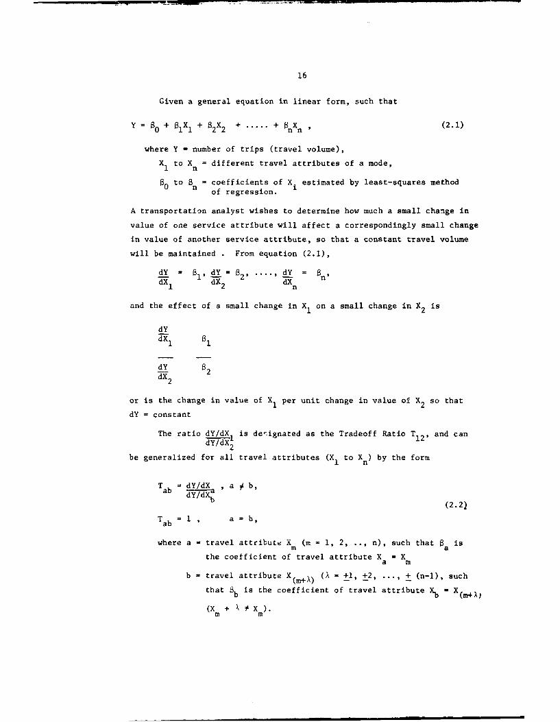
Given a general equation in linear form, such that

Y =0 + 61X1 + 6 2x 2 . ..... + anxn , (2.1)

where Y - number of trips (travel volume),

X1 to Xn = different travel attributes of a mode,

B0 to an = coefficients of Xi estimated by least-squares methodof regression.

A transportation analyst wishes to determine how much a small change in

value of one service attribute will affect a correspondingly small change

in value of another service attribute, so that a constant travel volume

will be maintained . From equation (2.1),

dY = 1, dY = 62 ..... , dY = nd i d X- -2 d-X1 n

and the effect of a small change in X1 on a small change in X2 is

dY

1 11

dY 6dX 2 2

or is the change in value of X1 per unit change in value of X2 so that

dY = constant

The ratio dY/dX is de ignated as the Tradeoff Ratio TI2' and candY /dX 2

be generalized for all travel attributes (X1 to Xn) by the form

T = dY/dX , a # b,Tab -

(2.2)

Tab 1, a b,

where a = travel attribute X (m - 1, 2, .. , n), such that B is

the coefficient of travel attribute X - Xa m

b = travel attribute X(M+X) (X = +1, +2, ... , + (n-l), such

that Bb is the coefficient of travel attribute Xb - X(mX)

(x + \ # x ).m

17

The Tradeoff Ratio as defined here is a rate of compensating change in

value of one travel attribute relative to another. It is the relative

importance or utility of a travel attribute in the eyes of the marginal

consumer when making a trip decision.

2.2 DERIVATION OF THE TRADEOFF RATIOS FROM AN ABSTRACT MODE FORMULATION

Qualitatively, the Tradeoff Ratio is a vlue which expresses how a

small change in value of one travel attribute will affect a correspondingly

small change in value of another travel attribute at some constant travel

volume. As applied to an Abstract Mode formulation, two different cases

must be examined:

Case 1 - Abstract Mode equations in linear form

Case 2 - Abstract Mode equations in exponential form

(linear in logs of the variables)

Case 1 - Linear Abstract Mode Equations

A general formulation of a linear Abstract Mode equation can be

defined as:

y 0 + RTXRT + ýBTXBT + 6RWXRW + $BWXBW + ORCXRCn

+ BCXBC + m m Xm1l

where XRT = Relative travel time by mode k between i and j

XBT = Best travel time by any mode between i and j

XRW = Relative walk time by mode k between i and j

XBW - Best walk time by any mode between i and j

XRC = Relative cost by mode k between i and j

XBC ' Best cost by any mode between i and j

X (m = 1,...h) - Environmental descriptors of the traveler, orm or nodes i and j

Ideally, the transportation planm'r or designer would like to express

the relationships that exist between various modal service and performance

attributes in terms of their actual values, rather than in terms of their

"best" or "relative" values, as defined by an Abstract Mode formulation.

18

In an equation such as (2.3), where actual values of each independent travel

attribute are not included, the following transformation can be made:

RELATIVE = ACTUAL / BEST,

or (2.4)

XRT ' XAT/XBT' XRW = AWB/XBw, XRC X AC /XBC'

where XAT = Actual travel time by mode k between i and j

XAW = Actual walk time by mode k between i and j

XAC = Actual cost by mode k between i and j

The "best" characteristic of a given travel attribute is independent

of the "actual" characteristic of that same attribute only when the

mode(s) possessing this value is not the "best" (fastest, cheapest, etc.)

mode(s) in that respect. When a mode possesses an actual value for a

travel attribute that is equal to the "bes,'" value by all modes, the"actual" and "best" values are dependent on each other.

In the case of dependence (XAT= = XBBW or XAC X BC), the

"relative" value is a constant (equal to one) for the mode whose

"actual" value for a given travel attribute is equal to the "best" value

by any mode for thaL •-e attribute. In the case of independence

(XAT XBT XAW 0 XBW, or XAC f 2,), when the "actual" characteristic

of a given travel attribute is being considered for a mode(s), the "best"

characteristic of that same travel attribute is a constant for that

mode(s), since the two values are properties of different modes. The"actual" value of the travel characteristic can change for this situation

without affecting the value of the "best" characteristic until the point

is reached where these values are equal. When these values are equal,

the "actual" characteristic is no longer independent of the "5est"'

characteristic, and the dependence situation exists.

The small change in value of one travel attribute relative to a

small change in value of another will yield a diffprent result depending

upon which situation, dependence or independence, exists between the"relative" and "best" values tor each travel attribute contained in an

Abstract Mode Formulation.

19

Situation 1 - Dependence

Dependence holds when the actual value of a travel attribute by

mode "k" between nodes "i" and "j" corresponds to the best (cheapest,

fattest, etc.) value by any mode between "i" and "j" (XAT = XBT, XAW = XBW,

or XAC - XBC). For example, if XAT ' X B, substitution of equation

(2.4) into equation (2.3) yields:

Y - 0 + $RT(XAT /XBT) + BBBT + BRWXRW + ...... (2.5)

and since XAT XBT,

Y - 0 + aRT + BTXAT + RWXRW +. ...... (2.6)

and

dY (2.7)dXAT BT'for XAT BT

Situation 2 - Independence

Independence holds when the actual value of a travel attribute by

mode "k" does not correspond to the best value (cheapest, fastest, etc.)

by any mode between "i" and "j" (XAT 0 XBT, XAW * XBW, or XAC 0 XBC).

For example, if XAT ý XBTV equation (2.5) still holds:

Y = B0 + $RT(XAT/XBT) + BBTXBT + 6RWXRW + ...... (2.5)

and XBT can be considered as a constant when differentiating with respect

to XAT, just as XRW, XBW, etc. are considered as constants. Therefore,

dY RB T B

dXT /X, for X # X (2.8)dXAT TBAT T

The same types of relationships for situations (i) and (2) will hold

for the walk time and cost attributes.

Since the tradeoff ratios with respect to out-of-pocket cost for

example, have been defined as:

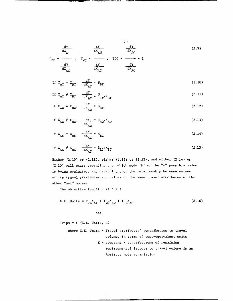
20

dY dY dY (2.9)dXAT dXAW dXAC

TTC T = , TCC= - 1

dY dY dYdXAC dXAC dXAC

if X X dY = (2.10)AT BT dXAT =BT

if X RT/B (2.11)XAT 3BT dXAT RT BT

if X X dY = (2.12)AW BW dX AW BT

If XAW X 8W, dY = aRW/XBW (2.13)dXAW

If XAC = XBC, dY =BC (2.14)XAC

dY a /x (2.15)If XAC #XBC, dXAC RC BC

Either (2.10) or (2.11), either (2.12) or (2.13), and either (2.14) or

(2.15) will exist depending upon which mode "k" of the "m" possible modes

is being evaluated, and depending upon the relationship between values

of its travel attributes and values of the same travel attributes of the

other "m-l" modes.

The objective function is then:

C.E. Units = TTCXAT I TwcXAw + TccXAc (2.16)

and

Trips - f (C.E. Units, k)

where C.E. Units = Travel attributes' contribution to travel

volume, in terms of cost-equivalent units

K = constant = contributions of remaining

environmental factors to travel volume in an

Abstract mode tormulation

21

Case 2 - Exponential (linear-in-log) Abstract Moae Equations

A general formulation of an exp-nential Abstract Mode equation can

be defined as:

8RT 8 BT xWBW • •B i •Y P aoXRT X 6BTXRW X 5BXRC BC XBC %CXi 1 -X (2.17)

where the variables and subscripts have the same meaning as in the linear

case. In logarithmic form, equation (2.17) could be expressed as:

logy = loga 0 + aRTIOgXRT + 5BTIOgXBT ++ aRWgXRw + %B•OgXBw

+ kClOgXRc + aBCIOgXBc + BilogXi + .. + amlogX (2.18)

Again it is desirable to work in terms of the actual values of a travel

attribute, rather than in terms of a travel attribute's "relative" or

"best values, so the transformations

RELATIVE - AVERAGE/BEST

or

XRT = XAT/XBTV XRW = XAW/XBW' XC = XAC/XBC (2.4)

are used. As in the linear case, two situations arise:

1. Dependence - the actual value of a travel characteristic for the

mode being considered is also the "best" value of that

same characteristic for any mode.

2. Independence - the actual value of a travel characteristic for

the mode being considered is not equal to the "best"

value of that same characteristic tor any mode.

22

Situation 1 - Dependence

(XAT - XBTV XAW ý XBW, or XAC - XBC)

For example if X = XBV substitution of (2.4) into equation (2.18)

yields:

logY - log%0 + aTl0g(XAT/XBT) + 6BTlOgXBT + B + . .... , (2.19)

and since XAT = XBT,

logY = log80 + BRTlog(l) + aBTlOgXAT + aRwlogXRW + -.. (2.20)

Differentiating with respect to XAT,

d(logY) BBTd(logX AT) /X for (2.21dXAT dXAT BT AT' XAT = XBT (2.21)

Situation 2 - Independence

(XAT 0 XBT, XAW # XBW, or XAC 0 XBC)

For this situation, if XAT 0 XBT, after the transformation (XRT - XAT/XBT)

is made, equation (2.19) still holds, or:

logY = loga0 + aRTIOg(XAT/XBT) + BTIOgXBT + RwOgXRw + .... (2.19)

Differentiating with respect to XAT,

d(logY) BRTd log(XAT/XBT)dX ATA -dX RT (xATXBT), forXAT XBT (2.22)dXA A

23

Again, the same types of relationships for sicuations (1) and (2)

will hold true for the walk time and cost travel attributes, giving rise

to the following tradeoff ratios with respect to out-of-pocket cost:

d(logY) d(loRY) d(logY)

dXAT dXAW dXACT = ____ , TWC _____ = =1i

TC T CC

d(logY) d(logY) d(logY)

dXAC dXAC dX AC (2.23)

If XAT = XBT d(logY) = aBT/XAT (2.24)dX AT

If XAT # XBT, d(logY) - aRT/(XATXBT) (2.25)

dXAT

If XAW = XBW, d(_oRY) - 8BW/XAW (2.26)

dXAW

if XAW X BW, d(logY) - RW/(XAWXBW) (2.27)

dXAW

If XAC =XBC d(logY) BC/XAC (2.28)

dXAC

If XAC # XBC' d(logY) = RC/(XACXBc) (2.29)dXAC

Either (2.24) or (2.25), either (2.26) or (2.27), and either (2.28)

or (2.29) will exist depending upon which mode "k" of the "m" possible

modes is being evaluated, and depending upon the relationship between

values of travel attributes and values of the same travel attributes for

the other "m-l" modes.

The objective function is then:

log (C.E. Units) = TTClogXAT + TWCIogXAW + TCCI ogXAC and (2.30)

log(Trips) = f (log(C.E. Units), log(K) )

24

2.3 THE TRADEOFF RATIO - IMPLICATIONS FOR TRANSP' RT PLANNING AND DESIGN

If the effectiveness of a transport system can be measured by volume

of travel, then

Travel volume = f(travel time, walk time, out-of-pocket cost, comfort, etc.)

is a measure of effectiveness which can be used in design. (2.31)

The transportation planner would like to provide a new system which

maximizes travel volume (consumer satisfaction) per dollar spent in

constructing, operating, and maintaining the facility. There are many

different combinations of the travel attributes possible, but the optimum

combination of travel attributes is that which maximizes the amount of

satisfaction (Travel Volume) obtainable from a given facility. The

tradeoff ratio is a measure of the relative importance of the system

attributes and therefore is a guide to selecting the satisfaction max-

imizing mix of attributes. It, in effect, tells the system designer which

performance characteristics should be changed.

A utility function such as equation 2.31 was not treated in any

further depth in this study, beyond its description here of its possible

significance in transport planning and design The author's intent was

to suggest the role the tradeoff ratio concept could play in a system or

network evaluation of alternative transportation facilities. Specific

tradeoff ratios were calculated, however, from the estimated Abstract

Mode formulations for the Boston Region (Chapter 3).

25

CHAPTER THREE

MODEL EVALUATION

3.1 THE ABSTRACT MODE MODEL - SUMMARY

Before expanding in detail the empirical results found in applying the

Abstract Mode Model to the Boston Metropolitan Area, general comments

can be made on the effectiveness of this model as a prediction device,

and as a tool, along with the tradeoff ratio concept, to analyze consumer

preferences and motivations in travel (and aid the planner in his search

and evaluation of system policy alternatives).

If the null hypothesis of this research study was that the Abstract

Mode Model can be used to predict demand for urban transportation, conclusive

evidence was not found to reject this hypothesis. The fitted equations

tended to indicate that either the particular travel parameters chosen

do not by themselves completely explain variations in consumer travel

behavior, or that consumer preferences in urban travel are random, and

cannot be fully described by the measurable attributes of a travel mode.

Poor statistical fits that did occur appeared to result more from sample

biases and aggregation problems inherent in the data base used, than from

the analytical concepts of the Abstract Mode Model.

Better statistical fits and significance were obtained from logarithmic

regressions than from linear regressions, adding support to Quandt and

Baumol's linear-in-logs hypothesis- In most cases, better fiL and sig-

nificance were obtained for those formulations having percent travel

volume by a mode as the dependent variable, rather than actual travel

volume by a mode, indicating that this model is better suited to pure

modal split rather than to both trip generation and modal split.

The model's use, along with the tradeotf ratio concepts, as a tool to

analyze consumer preference patterns, produced interesting results.

Consumer travel patterns were found to vary according to the time of day

in which the trip takes place In most regressions, good correlation

was found to exist between the cost variables and travel volume, while

little or no correlation was found to exist between the travel time

variables and travel volume, contradicting the generally accepted fact

that travel time is the single travel attribute which contributes the most

explanatory power to a travel demaml estimation prucedure, while out-of-

pocket cost exerts only a secondary inkluen-e

26

Calculating the tradeoff ratio of travel time with respect to out-of-

pocket cost from the regressions resulted in an average value of one

minute of peak hour travel time being equivalent to 5.8 cents out-of-pocket

cost. With this value, the dollar value a traveler places on his time

spent in peak hour travel was calculated, 3.48/hour. Placing more

importance on the general magnitude of this value rather than on its

specific value, leads to the conclusion that past estimates of the value

of a traveler's time, such as the minimum wage, may grossly understate

its true value. Furthermore, one hard and fast value cannot be placed on

a traveler's time,

The remainder of this chapter will be spend expanding and clarifying

the issues brought up in this section, The reader is asked to keep these

conclusions in mind as the discussion proceeds.

3.2 STATISTICAL EVALUATION - CONCLUSIONS

A comprehensive series oi regressions was performed, encompassing

many possible combinations of the 23 modal travel attributes and

environmental chara.teristics described earlier, in both linear and

logarithmic form, and for peak hour and otfpeak hour travel. The input

data was stratified on a subzone basis and on a town basis for origin-

destination zone considerations. It was further stratified by 6

specific travel modes (auto, auto driver, trackless trolley or bus,

subway or streetcar, tail commuter, and taxi), and also by the three more

general modes, auto, transit, and taxi. Tables 3.1 to 3.4 contain a

condensed listing of the key statistical quantities estimated for the

regressions, using survey data aggregated at the origin-subzone, destination-

subzone basis (148 subzones) and by the six specific travel modes, while

Tables 3.5 and 3.6 contain the same quantities estimated at the origin-town,

destination-town basis, and by the thiee general travel modes. The upper

value in each block is the variable's estimated regression coefficient

(B), and the lower value is the variable's computed "t" statistic for that

functional form. Below are listed the "R" and "F" values for each

functional form.

Because the total number of quantities estimated is very large, a

detailed evaluation of each of these quantities is beyond the scope of

this report, and would not reflect wh-,t the author sought to a-omplish

in this study. The level of derail t,- bh. empioNLJ in this evaluation, will

be in keeping with th* ie'- ion- th, authcr sought these estimates to answer,

tie 110i

Ywri j I 2.

-1.t62 162

-m n 3 f6f, C'

-. 04575 -.C4,A1 5 ft3 .ca; :t$

'kJ-3.513 -M.31 -3.437 -1.41? Ie6 1 -:z -.. 4 .07 .9

103.40-.4 -07 -A3 .17-fs

W=. 325 *.o5 5ý1 .396 . 67 .yC-If?

IIZI -0C7 .0G8 .017 -C076~ -. 039 .(192klj--,-7.-C-076 cC 0, .0 -002 .000.71 rf/37 . CtC .%5 .<714.'26i -4.245 -4.273 -4.i35 r1;7 .20C4 .205 .232 .271 .0Ž! 23 .:33

.- CLS.00125 .0CQ299 0 2.16 .00305 t-:1 74.N362i .210 -L6 .211 .121

-.21539

WS jr2 56,e -. 12%9

i -.00145? -- 00-'97 . A49 0

0-.5 ý 0 -. 5 32 * 3 .u 13

k -. 02752 24100

(AL .?t. C)% *j 1`3 1

Cr.usr .C /3 'C -2 t' C(,-6

.5)4 .475 .50 1 / 6 f5

.. 6124 .. 527 .4)2 -27C

7 12.097 7.30Žý 7.2,ro 5. A .31 1.• 1. 2. 1-; .9?r 1.02? i113 .9-1

28

Table 3.2

?Lak-I-nr to~jýrMt~Ac Eft:iir4c%4o

I MUR IT$ 7i?S kRIFS FIRIFS A¶JRUP8 ARIPS ATRIPS LTP1PS AT11IPS LflM.TS A'ZP.XS &!YP.!P

tr ON574 -. IW660 -. 09ý.40 -. 1073-. -. 'j96ijU .0712i .0?120 .11148 .Ce450 .C.ý'41 .108i2e .07962 .1013L&

kij .1I'3

(iL) -02573 -. 03337 -. C9fI& -- C2558 -22A40 .24517 .219378 t6' .25667 .;PL31 S .2c02 .2a.27-. :!41 *2- -;7 2~1 2.05f 1.659 2.1137 2. 1 90 1.ý42 e?)3 L.,E,

(flE12 ~ ~ .ý2 .27 -. 0, 0 -. 05 :.077 *C3S*Oz

tj-.O024 OC;4 CC7 .2!35 .01)26

W.05355 .o56L~6iij 1.816 1.91.0

Wav) kI.'l¶ -.O2-ý30 -. S02520 -. r02ý2 -0Z3 r*0726 .01672 .67397 .07556 .01912 o03JaL .07'417 .07517

W:f, ,53 51 .0L955 .05642 .05759 .051,13 .05"45I.161.677 1.939 1.938 1.794 1495L&

ý.M012 .oi

-. 3ss-.5

(Rzlc~r) k --.122t3 -.13"S -. 12339 -.132t. .02ý961 .01873 .C2156 .CI667 C.2717 .01603S .01751 .01711.0 .36ý -3.95113 -?.,-4 .25) .1-71 .571 f1.7 .63 .4415 .471 *45':

-35'7 -.287 -.455 -ýL9 -.436 -.4:9

.02171

r, 0)j -%16?6.066C5

(AlSIM)-.011C,4 -.0177 .0!9L.2 .06941-. )L,2 j.C .972 1.971,

i.Cz9 1.0642

.4S9 1.201 1.21,3

(!:C,.) I oz?!!A .,)22,5 -.572ý'7 .6'i -. Wt"'

.75619 4? � 6!<31 ~ .70V6c .722 (.¶ 6

1.163 1 ý 1.C. 12:, 1.11? 1.170

R .4?195 .4:ý .4.2276 . .25167 .35167 .4-321 L12925 .L2119 .397-11 .4~19 w,-133

r 12. Y 9 7.1ý7 7.617 9. 7•2.70M3 3.0341. r.0W'- - 3.162 1i"1~ 1 2.73"

29

table 3.3-

Cffitak-h"ar Line-ar ReCresalf'rh

I flIPS PTRIPB 1731-S gAsA -tPU-S3 i:A:s1:1 s Fln :?s' W?P'.1San.

CONSTAS? .822S-9 Ct271 S.2921 .S!402 1.571? 1.27fl,, 1.7C55 .7 1-7036 1.73326 :.17z-29 1-

(AUrT~j -. 01165 -. 01190-4.436 -. 6

CRBT~IJ-.5571 -. 05501 -. 05567 -. 5! 056 .16C35 .0171ý Oc.',g6 .14618 .02224 .C221L, .027?.7

-,.?26 -9.562 -9.719 -9.S59 .5115 31.21B .378 .210 2.r9~ h183 *L! .

tj-4.611 -4.612 -4.61-5 -4.58-0 -4.,<1 -4.703

(An-'T) kii -. cc,613 .04-. 1-,- -1.180

(RZLVZ1) -. 00-219 -.oz16 -7.P0218 -.00223 V,03L6 .0:3;5 C003C4 .C-293 .(0037- .3261 .G02-,z .0o!j,6

kJ-.654 -$.439 -5.602 -S.?- 1.717 1.606 1.411 1.2,c7 1.714 1.5?4 i.30 1.672

W w? -. 00,115 -.cTO.75 -.ooSC6 -. 005ý5 -.0117! -.00171

..& -'171. -. 'ý1 744 -. ?33 .3

Or-.0C ) -. Ct1130 -. O00030 -. 00030 -. ýOtf -.031- -.0C0le fM 00Cr:22 -rco16 - .00020-.(1

-. 652 -9.55B -9-652 -3.6-2 - /4 -. 476, -. 714 - .2 65 -1 .3

.5'PLI '03 .tt.rIt('Z- .7

(A--Okj.0I 3 6 -. 116t0-1.r.27-25

.942: 00225

1 * 1461346

(AUVLIC) 1 -/5412

5.419

6,') 554 6. 6i 1 122 *ý; .1-9 . .7Ž6 1.'2t,

8667. 3.F31 1C . ' 2-l 5.: 1.~ !'1:

-. 25Ž

3 .3-/)20 .3!9I-S 0!:^3 .3i327;.2 .1 ~56 .7- . 0 .2,411

~~o~~tl 3'r, C!cr~

30

Able1, 3.14

Offpe.k-bour L-&%rtth.tc R*orresplons

T PTRIPS FlPIF$ PRIFS M1?17$ A01Z-$IS $ TP15 ATjRIPS ARIPS A81111$ ATRIPS ATRIPS AYIRPS

COISTA..T -. 114763 -. 14702 -. 15120 -. 1S269 .22V;3 .22505 .231C3 .21265 .21272 .23667 .20570 .29238

(AV31)i, -. 124J.5 -. 12068-6.P59 -6.549

(R•!iL)J -. 2%W, -. 23M65 -,29' -,:•.." .1974? .67671 Co677 .18136 .C6953 06774 .06305-8.709 -8.662 -S.7C4 -9.003 ,.s2 5.720 2.139 1.896 5.449 1.945 1.901 1.785

(Z$TI4)1.I -. 12•40 -. 12L.90 -. 12063 -. 12580 -. 12174 -. 12627-5.856 -6.778 -6.546 -6.620 -6.595 -6.e97

(AvrýT)klj .010) .008681.297 1.044

wl*) kii :j-.03177 -.03201 -. 03193-.03108 , .07ý' .066420 ,C'515 .07232 .06364 .0?525 .07320 .07101-2.93 -2.815 -2.802 -2.7122 6.t416 4.630 6.434& 6.195 4.800 6.435 6.274 6.138

(M,..T) .01077 .01183 .00oc .01124. .COE69 .011171.294 1.420 1.0L1 1.347 1.045 1.356

(A=T) kI .00455 .00407.753 .663

(E2LCTk -. C8e46 -. 0•419 -. 0E461 -. C-!ý25 -. 0t861 -. 01306 -. C0499 -. 00825 -. 01233 -. 00615 -. C099! -. 01250-10(o.0? -10.49ý9 -10.752 -11.320 -1.052 -1.41,4 -. 607 -1.004 -1.337 -1.0^? -1,.235 -1.560(ESSTCT)I ,Cs55 ,oC791 .00,O0 ,0C5e6 .00035 .00232

U.755 1.278 .664 .943 .137 .388(.PýD-,Ukjj-.O0053

-. 292( AIomit) tjt)0

CAIO) ktj -. tP8925 .02612

-11.319 2.247

(AIAUT0)IJ .00990M76

(A!?iCo-)klj .00304 XO3 .03114 .03114..405 L'07 4.063 4.02

-f'cm) t. •.02563 .026792.907 3.C67

'DLIC) .00502 -. 01108 -. Cll

(ALLC) tj -. 04239-2,895

(r0?) ro~. go . -39 .."??7-.' .9? .05S C71.", 1.4~D -1.171 -1,• -1.156 -1.1Z5 -1.171 -. 5-;6.o0 .9 .oC.? .00246 0,n1 '3 .c,'T 171 9 5 ."0113 -. V.2432.072 2.072 .12? .,c, rgc .:i .(,59 .127

(v*noy)! 1.015^6 OIL1%2 .01•• 02 4 .01294 ,0!2"•

1.~1. . 1.75'. 1.7-IL 1.!A3 1.540(r.'i-LOT)j .00%•4 .0 L- .f'r2 .C(7ý1 .9076. ,

.319 -.9 3 . 7 .33 .490

R 43 .43 .4 32 *37 ''i ? i. ' "( .2636. .- - 25 .29k.58

18S'1 'c . "? 93 r'., 1ý.. '9 - .,-.t5 IL.?,

-31-

a~~ ChaIn 1

N 1010 -.~ 0 -7'- m%0 1 nO

60~a "' 9 nN0

goN 0 4%nN 10 0 0 . 0 I

60 01I 0% 10 o

00 ccN

In N. n 1 -40401 0 N I

I~b NI N 0N N .w*ON O N N IPC41

o~~~~~0 4w0N* N N N. I.

-32

0.~G 0% 40 0 .400

1-I ~ ~ ~ ~ ~ . co011 .0 1 ., 0 0 . .4 .4 '00.-. 0.

4

In1 0-0.a

N. 0 00- IM In4.411 1*.0 0 0 .0 N.4 N O.00~ ~ ~ ~ ~ ~ ~~a 00 1- 0 0r- 4 . .~ 0 n 0 q 9 .IIt 0 0

0. o1- * N a ,0 0 I ' 0 ). 4 *.4 ' NN a WNl 10 do' t io co'l ~ u . . -

00 6m1.40

Ch . h 00 '7

In

Mn 0 0

O N . 0 .Q l * C C~ l . 4 0 . 4 1 1 r ' l . 0 ' 4O N

* - 01 .4 .1. 0 1.4 ..- 4 1-

0110 4

1.9

* Go

0o 44 IO) 0 3Io ' .. 0 4 4 '. C . 4 1 4 1 1 1 0 >.

0

mw

33concerning the Abstract Mode Model and consumer [-eference patterns in

urban travel.

Better fit ("R" values) and significance ("f" values at 99% confidence

interval) were obtained in all cases from the logarithmic regressions

than from the linear regressions, adding support to Quandt and Baumol's

linear-in-logs hypothesis. Better fit and significance were also obtained

using PTRIPS (percent of trips by a mode) as the dependent variable, rather

than ATRIPS (actual number of trips by a mode) indicating that this model

is better suited to pure modal split rather than to both modal split and

trip generation (refer to Table 1.1 for definition of PTRIPS and ATRIPS).

Finally, better fit and significance, in most cases, were obtained from

those regressions using input observations aggregated on an origin-town,

destination-town, 3-general-modes basis, than from the same data aggregated

on an origin-subzone, destination-subzone, 6-specific-modes basis.

The author hypothesizes that to some extent, the low "R" values reflect

the fact that consumer preferences in urban travel cannot be completely

explained by the measurable attributes of a traveler or of the travel

mode he chooses. Factors such as privacy and comfort also play important

roles in influencing the trip-making decisions of a traveler, If these

subjective elements could be quantified, the trip-decision process would

be better explained. Constraints imposed by the availability of data and

the amount of data manipulation involved, prevented the author from

including these subjective elements in his analysis ot the Ab,ýtract Mode

Model, except for the use of walk times to and from a mode as a measure

of convenience. The problem of evaluating factors such as privacy, comfort,

and convenience is difficult to solve when secondary data sources are

used (sample data collected by study groups other than the individual who

is using the data, and not intended for the individual's specific purpose.

The author further contends that the poor correlation (accuracy) which

resulted in all regressions performed on the subzone data (Tables 3.1 to

3.4) was due to the manner in which these observations were aggregated

and used, rather than from the explanatory variables and formulations

chosen. Examination of the means of the dependent variables, PTRIPS or

ATRIPS, from these regressions add support to this argument. For the

peak-hour and offpeak-hour linear regressions, the values for the mean

of ATRIPS were 1.945 and 1.723 respectively, indicating that the average

input observation consisted of less than two trips by a mode. In effect,

34

modal choice was practically non-existent, Further examination of printouts

of the person-trip observations aggregated by origin, destination, and

mode showed that a good many consisted of only a single trip by a single

mode between a given O-D pair (ATRIPS - 1.00). The result was an attempt

by the varying explanatory variables in a given functional form to explain

little or no variation in the dependent variable (PTRIPS or ATRIPS), or

low "R" values (poor statistical fits). Modal split cannot be explained

when little or no modal split has been recorded. Variation in travel volume

cannot be explained by a sample biased toward uni-modal, single-trip

observations.,

This hypothesis of poor fit because of poor data aggregation prompted

the author to reaggregate the same data one level higher, on the town

basis and by the three general urban travel modes. The better results

(Tables 3.5 and 3.6) juqtifled this additional data manipulation, and

further pointed out the exacting data structure demanded by the use of the

Abstract Mode Model.

From Tables 3.1 to 3.6, it can be seen, especially for the ATRIPS

functional forms, that adding more independent variables to a given

functional form does not significantly improve the ocrrelation in the

new functional form created. Also, better correlation was obtained for

a functional form containing the "BEST" values of given travel attributes

than for the same functional form containing the "ACTUAL" values of the

same travel attributes in place of the "BEST", indicating that the

Abstract Mode method of using absolute impedences to travel was at least

as good as methods employed by other models.

In conclusion, if the null hypothesis of this thesis (H0 ), was that

the Abstract Mode Model can be used to predict demand for urban transporta-

tion, the author did not find conclusive evidence to reject that hypothesis.

Data structure and the randomness of consumer travel patterns influenced

the nature of the results obtained. Good corielation was obtained for

logarithmic regressions using input observations aggregated at a town

basis, the "R" values varying between 0.83 and 0.88. All these functional

forms were si. ificant at a 99% confidence interval or greater ("F" values).

The estimated regression coefficients (B's) of the independent

variables used in the Abstract Mode formulations were as expected in some

cases and contrary to those expected in others.

35

For the travel attributes, the most unexpected result was the large

contribution to the explanatory powers of an estimated equation the cost

variables provided, while the travel time variables contributed little or

no explanatory power to a given estimated equation. Table 3.7 affords

a comparison of the simple correlation coefficients of the travel attributes

("r' values) for the peak-hour logarithmic regressions calculated at an

origin-destination-town basis.

Table 3.7"r" Values - Logarithmic Peak-hour Regressions,

Town Basis

Travel Time Walk Time Out-of-Pocket Cost

AVET 0.02 AVEWT 0.55 AVECT -0.53

BESTTM 0.04 BESTWT 0.21 BESTCT 0.15

RELT -0.01 RELWT 0.53 RELCT -0.62

This result is contrary to the generally accepted notion that travel

time is more powerful than travel cost in explaining trip-making patterns

and modal choice. 1 2 ' 2 1 ' 2 2 ' 2 7 ' 2 8 That cost was more important than time

in all regressions performed in this study makes the author cautious in

interpreting its implications. If one has knowledge of the study area

the author's data encompasses, and, keeps in mind some of the peculiarities

present in the data (Chapter 2), a plausible explanation of this unexpected

result emerges. Boston, like many older cities in this country, has a

well established transit system, especially within the study area chosen,

both onstreet (bus, trolley) and offstreet (rapid rail, railroad commuter,

trolley). A densely populated area with high daily travel volumes by all

modes exists. The results, especially during the peak hours, are low,

near-equal values of travel speed (high values of travel time) for auto,

taxi, and transit for on-street travel.6,28 For offstreet travel, since

station spacings are more closely spaced for rail transit serving dense

urban areas than for less-dense areas, transit travel times are increased

(speed decreased), decreasing the exclusive-right-of-way advantages of

rail transit. Offstreet vehicle travel times closely approximate on-street

vehicle travel times in this high-density area, resulting in little or

no variation In travel times between competing modes (low "r" values when

correlated against tt.ivel volume).6,28

36

As mentioned in Chapter Two, the fact that many person-trip observations

contained zero values of out-of-pocket cost for the auto modes, moderate

values of out-of-pocket cost for the transit modes, and high values of

out-of-pocket cost for the taxi mode, would result in significant variations

in out-of-pocket cost between the competing modes. When correlated against

travel volume, where auto trips dominate over transit trips, and transit

trips dominate over taxi trips, the result would be high "t" values for

the cost variables.

Another unexpected result was the fact that the signs of the walktime

variables consistently were contrary to that expected (positive), since

one would expect travel volume by a mode to increase as the walktimes to

and from that mode decreased (negative sign). The only explanation

offered to account for this result is the fact that, transit trips are

more prominent than auto trips or taxi trips for trip-ends more closely

spaced in a high-density area, because transit is more readily available

and is more convenient. As the distance between trip ends increases,

direct transit service between these trip-ends is usually less established

and less frequent, making the auto mode more desirable. The travel volume

between more widely spaced trip ends is usually less than the travel

volume between more closely spaced trip ends. Since the former type of

trip is usually undertaken more by the auto mode than by the transit mode,

the auto mode implying lower values of walktime than the transit modes,

the result could be a positive correlation between walktime and travel

volume, travel volume decreasing as walktime decreases, and vice versa.

In summary, travelers do not regard walktime and out-of-pocket cost

as costs when traveling by the auto mode Because of tiis, high negative

correlation was found to exist between out-of-pocket cost and travel

volume, while high positive correlation was found to exist between walktime

and travel volume. Because of the relative insensitivity in value of

travel time between alternative modes, low correlation was found to

exist between travel time and travel volume. In general, the "relative"

travel attributes possessed better fits ("r" values) and significance

("t" values at 99% confidence interval) than the "best" travel attributes.

The regression coefficients (O's) were fairly consistent from one

functional form to another within the same regression, indicating no

problems of multicollinearity existed. Contrary signs existed the most

for the walktime variables

37

For the subzone regressions, it was desirable to ascertain whether

the regression coefficients (W's) of each variable from two different

sample populations (peak and offpeak) were the same for all practical

purposes, indicating that consumer preference patterns do not change at

different times of the day.

The null hypothesis, H0 : B1 = B2, was tested against the alternativehypothesis, H1: 6I 0 ý2, at a 95% confidence interval (+ t95 + ±1.96).

The result was that the difference between values for the same regression

coefficients estimated for the peak-hour and offpeak-hour samples was

negligible for many of the \TRIPS functional forms (reject H1 : 8i # Y)

indicating that consumer preference patterns do not differ significantly

over time. Four of the six possible cases for the PTRIPS functional forms

had significant differences in the mean values of their regression

coefficients (reject H0 : B1 = B2), indicating that consumer preference

patterns do differ over time. Siace the PTRIPS functional forms possessed

better fits and significance than the ATRIPS functional forms, along with

more correct signs for the variables regression coefficients, the author

contends that the evidence was sufficient enough to conclude that consumer

preference patterns do vary over time (reject H0 and 81 a82.)

For the environmental descriptors of the tra\oeler and trip ends, the

population and employment variables were found to contribute little or

nothing to the explanatory power of an estimated equation for all the

regressions performed (low "r" values) In many cases, their estimated

regression coefficients (W's) possessed contrary signs (negative instead

of positive) and were not statistically significant at a 90% confidence

interval or greater.

For the environmental descriptors of the traveler, the driver's license

and auto ownership variables computed on the per-mode basis (DLK and AUTO)

contributed the most explanatory powers to an Abstract Mode formulation

for all regressions performed (high "r" values), consistently were sig-

nificant at a 90% confidence interval or greater, and had signs as

expected (positive) in most cases. In general, those variables computed

on a per-all-modes basis (ALNODR, ALAUTO, ALDLIC, ALINCM) possessed

lower "r" values, more contrary signs, and -ower "t" values (significance)

than did their counterparts calculated on a per-mode basis (ANODRI,

AUTO, DLIC, AINCOM)

38

3.3 STRENGTHS AND WEAKNESSES OF THE MODEL

The strengths and weaknesses of the Abstract Mode Model uncovered in

this research investigation center, in one way or another, around the

model's data requirements.

This model, as stated by Quandt and Baumol, does minimize the effect4

of incompleteness of data . Observations for all modes between a given

origin zone-destination zone pair were not prerequisites for the use of

this model, nor were observations for all origin zone-destination zone

pairs. By characterizing a mode in terms of values of the several variables

that affect the desirability of the mode's service to the public, such as

travel time, walk time, and out-of-pocket cost modal neutrality and trip-end

neutrality is observed. The model assumes that a person chooses among

modes purely on the basis of their observed characteristics. Trip-ends are

characterized by impedence factors ("best" values of each travel attribute

between an O-D pair) for travel time, walk time, and cost and by environmental

descriptors such as population and employment levels.

Another strength of this model, because of its modal neutrality, is

that the end result desired from the estimation of an Abstract Mode formula-

tion, a travel demand predictive capability for the area under consideration,

can be applied to any mode, present or future (hence the name "abstract

mode"). As pointed out in Chapter One, this predictive capability will

become most important in the future as planners and designers look to

new travel modes to solve the ever-increasing urban transportation problem.

Finally, a strength of the Abstract Mode Model, perhaps not too

evident at this time, is its use in evaluating consumer preferences in

urban travel. It was hypothesized earlier that the measurable attributes

of a mode can be used to analyze consumer travel patterns. Since the

Abstract Mode Model preserves modal neutrality, in the sense that all

present or future modes are "abstract", the estimated regression coefficients

in a given formulation represent a cross-section of the observed travel

behaviors of a heterogeneous population using a variety of alternative

travel modes. Section 3.4 illustrates the model's use, along with the

tradeoff ratio concepts, in evaluating consumer's preferences and motiva-

tions in travel.

39

A major weakness of this model, for urban areas at least, is the

massive data requirements, and subsequent data manipulation capabilities,

demanded by this model, When secondary data sources are used, such as

the 1963 BRPP home-iLiterview surveys, the data is often far from the

form required by the model, and is often inadequate in scope. To cite

the author's 14,000 peak-hour, person-trip observations for the study

area under consideration were extracted in unordered form from three

magnetic computer tapes containing 133,000 total person-trip observations.

These observations had next to be sorted by origin, destination, and

mode, and by destination, origin, and mode. Once sorted, the person

trip observations for each origin subzone, destination subzone, and

specific travel mode were aggregated, mean values of each variable cal-

culated, the "best" values of each travel attribute for each O-D pair

computed, the "relative" values computed, and finally the resulting

values output as a single observation to the Abstract Mode Model.

Though these steps may seem relatively straightforward, especially

since they were performed on a computer, the computational time and effort

involved far exceeded that of the other task done in this study. The end

result was that 14,000 observations were insufficient to describe trip-

making at the subzone basis (Tables 3.1 and 3.2) and further manipulation

was involved to reaggregate the data at a higher level, on a town basis,

and by the three general travel modes. Better regressions were obtained

but also increased generalization due to the higher-level aggregation.

Finally, perhaps not a weakness in the true sense, is the fact that

an Abstract Mode equation is estimated by regression techniques, requiring

that the input data be amenable to regression. Regression techniques

fail if there is little or no variation in the dependent variable (in

this case, travel volume for the subzone regressions), or there is little

or no variation in value of the independent variables with variation in

value of the dependent variable (travel time, for example). Since less

variation in value often occurs in intra-city travel for travel attributes

than for inter-city travel, and due to other peculiarities often found

in the survey data (zero values for walk time and cost for the auto

modes), the real world situation cannot always be accurately predicted

by regression. To obtain variation in the dependent variable, travel

volume, it is often necessary to either aggregate the trip observations

at a different level (town basis in this study) or to secure an unduly

40

large data base ( '>14,000 person-trip observaticns in this study). It

would seem advisable to consider other models in preference to the Abstract

Mode Model when these conditions exist. The Abstract Mode Model was

designed for inter-city travel, where the data problems described above

are minimal. It can be used for intra-city travel, and is effective, if

one is willing to undergo the time and effort that may be involved in data

acquisition, aggregation, and manipulation.

3.4 MODEL RESULTS PLUS TRADEOFF RATIOS DESIGN IMPLICATIONS

For analysis purposes in transportation systems design, it would be

meaningless to compute the tradeoff ratios from regression coefficients

of travel attributes which possessed signs contrary to those expected,

and which were not significant or reliable in explaining variations in

the dependent variable, travel volume by a mode. These two situations,

contrary signs and insifnificance, were present in many of the estimated

equations for the subzone regressions, peak-hour linear and log, and

offpeak-hour linear and log. The result was that no meaningful tradeoff

ratios could be computed from these regressions, in terms of regression

coefficients with both expected signs and statistical significance at a

95% confidence interval or greater. A similar situation existed for the

peak-hour, linear, town regressions, and for the walk time variables

(contrary sign for 6's) in the peak-hour, logarithmic, town regressions.

However, in the latter regressions, the travel time and out-of-pocket

cost variables consistently had B's with signs as expected (negative),

and which were significant at a 95% confidence interval or greater.

To illustrate the calculation of the tradeoff ratios from a given

Abstract Mode formulation and their meaning in the context of transporta-

tion systems design, they were computed for travel time and out-of-pccket

cost from the peak-hour, logarithmic, town regressions. Their development

also leads to one final consideration always of interest to the planner -

the value of time spent in travel.

Ir. errospect, the Tradeoff Ratio is defined as the ratio of com-

pensating change in value of one travel attribute relative to another at

a constant level of travel volume or for travel time and out-of-pocket

cost:

41

Linear Linear-in-Logs

dY d (logY)

dX dX-AT -AT

TC dY d(log Y)

-XAC -EAC

Where Y - travel volume

XAT = actual value of travel time

X• actual value of out-of-pocket cost

Using the expressions for the tradeoff ratios derived in Section 2.2,

the tradeoff ratios between travel time and out-of-pocket cost were

computed from the peak-hour logarithmic, town regressions for each of

the seven trip generation-modal split abstract mode formulations

(Table 3.8).

Table 3.8

Computed Tradeoff Ratios for Travel Time and

Out-of-Pocket Cost-Logarithmic Town Regressions

XAT -XBT XAT =XBT XAT #XBT XAT #XBT

XAC X BC XAC X BC XAC B BC XAC XBC

Selection TTC TTc TiC Ttc

4 5.65 3.54 0.37 0.26

6 6.20 3.52 0.45 0.26

7 4.76 3.68 0.32 0.25

8 5.54 4.57 0.35 0.29

9 9.37 5.25 0.46 0.26

10 4.70 3.50 0.33 0.25

11 4.27 3.43 0.28 0.22

Mean 5.80 3.93 0.37 0.26

42

Since a planner would like to design a travel mode which offers the least

travel time and out-of-pocket cost to the consumer, and should thus generate

maximum system use, the pertinent tradeoff ratios to be examined here are

contained in Column One of Table 3.8, where TTC = 5.80.

If one is willing to recognize that a negative-exponential (linear-

in-logs) relationship exists between travel time and out-of-pocket cost

and travel volume, the computed tradeoff ratio of travel time with respect

to out-of-pocket cost can be directly used to determine the value of a

consumer's time spent in travel. In terms of its proper units,

dY

dxA trips-AT cents

TTC = = minute =

dY minute-- trips

dx_ cent-AC

Therefore T = 5.8 cents 60 minutesC miuex 1 or = $3.48/hourmi~nute x1 hour

Viewing this hourly rate of $3.48/hour as even just a rough order

of magnitude, one can realize that it far exceeds AASHO's standard estimate

of $1.55/hour for the value of consumer time spent in travel. This value

is for those individuals using the "best" mode with respect to both

travel time and cost. For those individuals using the mode with the

lowest travel time but not the lowest cost, the rate is still higher than

AASHO's or is $2.36/hour (Column 2, Table 3.8). Quite understandably,

individuals who use a mode which does not possess the lowest travel

time, place a different (and lower) value on their time spent in travel

(Columns 3 and 4, Table 3.8).

The preceding observations lead to the conclusion that one hard and

fast value cannot be placed on a traveler's time. If an individual has

the financial and locational means to choose between competing modes, he

will usually choose the mode which offers him the best service. In terms

of travel time and out-of-pocket cost, he will usually choose a mode which

minimizes a weighted tunction of both, of these travel attributes. If

43

this be true, Column one of Table 3.8 is the ideal tradeoff he would like

to make betwee- time and cost, which means he values his time spent in

travel more highly than previous "one-shot" estimates such as AASHO's

or the minimum urge tend to indicate.

SUMMARY AND CONCLUSIONS

The effectiveness of the Abstract Mode Model as a prediction device

in urban areas and as a tool with which to analyze consumer preferences

and motivations in urban travel was tested by applying it to the Boston

Metropolitan Area. An extensive series of regressions were performed

to test the model's effectiveness, requiring a large amount of data

collection, manipulation, and aggregation. If the hypothesis of this

study was that the Abstract Mode. Model could be used to predict trip

generation and modal split in urban areas, this hypothesis could not

be rejected.

Poor statistical fits that did occur appeared to result more from

sample biases present in the data base used, rather than from the analytical

concepts ot the Abstract Mode Model. Moreover, the fitted equations

tended to indicate that either the particular travel parameters chosen

do not by themselves completely explain variations in consumer travel

behavior, or that consumer preferences in urban travel are random, and

cannot be described by the measurable attributes of a mode.

The Abstract Mode formulations were found to possess better fit and

significance in exponential form (linear-in-logs) than in linear form,

and the model was found to be better suited to pure modal split than

to both trip generation and modal split.

Finally, with the aid of the tradeoff ratio concepts developed in

this study, the Abstract Mode Model was found to be effective in analyzing

consumer preferences and motivations in urban travel. More specifically,

tradeoffs that existed between travel time by a mode and the out-of-pocket

cost to travel on Zhdt ,.ode were established. From these tradeoffs, the

value the consumer places on his time spent in travel was calculated, and

found to be higher than previous estimates of this value tended to

indicate, such as the minimum wage. It was also found that one hard and

fast value could not be placeid on a consumer's time.

44

Approaching trip-making and modal distribution from the consumer's

viewpoint is a method seldom utilized because it involves analysis of

human behavior both rational and irrational. One cannot begin to enumerate

the many intangible factors which influence an individual's trip-making

decisions - privacy, comfort, convenience, noise, social status, aesthetics,

etc. Many of these factors cannot be taken into account in a transportation

demand model, while others can be approximated in terms of the measurable

attributes of a mode.

In conclusion, the author recommends that any future research con-

ducted on the Abstract Mode Model should consider the following issues.

When the analyst cannot collect his own data in the form he requires it,

careful use should be made of secondary sources, such as the 1963 BRPP

Home-Interview Surveys, Origin and destination zones must be selected

where the analyst knows that there is a choice between alternative modes,

and that trip observations by these modes have been recorded. The level

of aggregation used should be in keeping with the accuracy of the predictive

estimators desired, and at a minimum, would be desirable on a town basis

for urban travel.

SeconJiy, sample breakdown should be in keeping with the classes of

travelers to be analyzed. In this research study, subdivision of daily

travel into the peak hours and offpeak hours appears justified, because

the regressions tended to indicate that consumer preference patterns

varied over time. The computation of the tradeoff ratios (Section 3.4)

pointed out the fact that the traveler values his time spent in travel

highly. The author contends that the value he places on his time will

vary with his income level, which would suggest a sample breakdown by

at least general income groupings (low, medium, high). Breakdown by

trip purpose, work and non-work, also appears desirable.

Why does a person take a trip? Why does he choose mode "X" rather

than mode "Y"? Why does he value one travel characteristic more highly

than another" A few questions such as these have been answered in varying

degrees by this research study. Many have been left unanswered. Only

future research by tle author and others will provide answers to these

questions.

45

BIBLIOGRAPHY

1. Armstrong, Richard S., The Relationship of Trip Demand to Socio-EconomicCharacteristics in the Boston Region. Masters of Science Thesis,Course I, May 1966.

2. Balek, a.j., Feital, M. J-, Sevin, A. F., and E. Weiner, Modal Split.U.S. Department of Commerce, Bureau of Public Roads, Office ofPlanning, December 1966.

3. Baumol, William J., and Richard E. Quandt, "The Abstract Mode Model:Theory and Measurement-" Northeast Corridor Transportation Project,Technical Paper No- 4, U.S, Department of Commerce, June 1966

4. Baumol, William J., and Richard E. Quandt, "The Demand for AbstractTransport Modes: Theory and Measurement." Journal of RegionalScience, Volume 6, No. 2, pp. 13-26, 1966.

5. Brunk, H. D., An Introduction to Mathematical Statistics. Ginn andCompany, New York, N.Y., 1960.

6. Comprehensive Traffic and Transportation Inventory. Boston RegionalPlanning Project, Wilbur Smith and Associates, New Haven, Connecticut,1965.

7. Coding Manual Boston Regional Planning Project, Wilbur Smith andAssociates, New Haven, Connecticut, 1965.

8. Deen, T. B., Mertz, W L., and N.A. Irwin, "Application of a ModalSplit Model To Travel Estimates for the Washington Area."Highway Research Record No 38, pp. 98-127, 1963.

9. Foote, Richard J., "Analytical Tools for Studying Demand and PriceStructures." U.S. Department of Agriculture, Agriculture HandbookNo. 146, Washington, D.C., August 1958.

10. Freund, John E , and Irwin Miller, Probability and Statistics forEngineers. Prentice-Hall, Inc., Englewood Cliffs, New Jersey, 1965.

11. Hill, DM , and H G. Von Cube, "Development of a Model for ForecastingTravel Mode Choice in Urban Areas." Highway Research Record No. 38pp 78-97, 1963.

12. Hille, S J. and T K Martin, "Consumer Preference in Transportation".Highway Research Record No 197, pp. 36-44, 1967.

13. Hoel, Paul G., Elementary Statistics, John Wiley and Sons, Inc.,New York, N.Y , 1960

14. IBM System/360 Operating System Sort/Merge. Program Number 360S-SM-023,International Business Machines Corporation, Poughkeepsie, N.Y., 1967.

15. IBM System/J60 Scientific Subroutine Package, Programmer's Manual.Program Number 360A-CM-O3X, International Business MachinesCorporatlcn, Poughkeepsie, N.Y. , 1966.

46

16. IBM System/360 Basic FORTRAN IV Language. International BusinessMachines Corporation, Poughkeepsie, N.Y., 1966.

17. Inventory and Characteristics ct Public Transportation Facilities.Boston Regional Planning Project, Wilbur Smith and Associates,New Ha~en, Connecticut, Volumes I and II, 1965.

18. Johnston, J., Econometric Methods. McGraw-Hill Book Company, Inc.,New York, N.Y., 1963.

19. Kissin, John, "The Demand tor Bus Travel." Studies in Travel Demand,Volume I, MATHEMATICA, Princeton, N.J., pp. 99-125, September 1965.

20. Lancaster, Kelvin J., "A New Approach to Consumer Theory." The Journalof Political Economy, Volume 74, No. 2, University of ChicagoPress, April 1966.

21. Martin, B. V., Memmott, F. W., and A- J. Bone, Principles and Techniquescf Predicting Future Demand tor Urban Area Transportation. M.I.T.Report No 3, M.I T. Press, Cambridge, Mass., 1961.

22. Meyer, Kain, and Wohl, The Urban Transportation Problem. HarvardUniversity Press, Cambridge, Mass., 1963,

23. Monsud, Solit,, "hu Dt':.,And for Railroad Travel". Studies in TravelDeiand Volume , VoII TI.rCA, Princeton, N.J., pp. 127-164,September 1965.

24. MBTA: Pzogram for Mass Transportation. Massachusetts Bay TransitAujthoz'tv Boston, Mass., August 1966-

25 MBTA: Stinf SLEpiementan __yReport to the Program for Mass TransportationMssa~husetts Biy Transit Authority, Boston, Mass., August 1966.

26. McCracken, Daniel D , A Guide to FORTRAN Programming. John Wiley andSons, Inc., New York, N Y , 1961.

27. Oi, W.Y , and P.W Shuldiner, An Analysis of Urban Travel Demands.Northwestern University Press, Evanston, Ohio, 1962.

28. Owen, W. , The Mett polittan Transportation Problem. Doubleday andCompany, Inc., Garden City, New York, 1966 (revised).

29. Plourde, Rodney P., "Cc¢muter Pieferences as Affecting the ModalDiLt:ibbtion -r Trips by Purpose in Urban Areas." Term Paper,CsGrse 1 213, M I T , Fall Term 1966 (limited circulation).

30. Plourde, Rodney P . "Consumer Preferences and the Abstract ModeModel: Boston Met~oplitan Area " Discussion Paper T-23, M.I.T.Ciiji Engineering Dept., Transportation Systems Division, October1967 (limited citz-.lation).

31- Plo..rde, Rodnty P . Progrins lor the Manipulation of the 1963 BRPP"02" Srve•_tapes M.1 I dAvil Engineering Dept., TransportationSystems D)ivisin. ,Cxirue I il1, Fall Term 1967.

47

32. Print-outs, 1963 Survey Data - Eastern Massachusetts Region. BostonRegional Planning Project, Alan M. Voorhees and Associates, Inc.,Washington, D.C., 1965ý

33. Quandt, Richard E., "The Construction of Travel Demand Models withIncomplete Data-" Papers - Seventh Annual Meeting. TransportationResearch Forum, Richard E. Cross Company, Oxford, Indiana,pp. 115-121, 1966.

34. Quandt, Richard E., "Tests of the Abstract Mode Model." Studies inTravel Demand, Volume II, Northeast Corridor TransportationProject, U.S. Dept. of Commerce, pp. 32-46, September 1966.

35. Quandt, Richard E., "A Probabilistic Abstract Mode Model." Studiesin Travel Demand, Volume II, Northeast Corridor TransportationProject, U.S. Dept. of Commerce, pp. 90-113, September 1966.

36. T:ansportation and Parking for Tomorrow's Cities. Wilbur Smith andAssociates, New Haven, Connecticut, 1966.

37. Plourde, Rodney P., "Consumer Preferences and the Abstract ModeModel: Boston Metropolitan Area." Master of Science Thesis,Massachusetts Institute oi Technology, Department of CivilEngineering, Febrdury 1968.

48

APPENDIX

LIST OF FIGURES AND TABLES

FIGURES Page

1.1 Study Area ......... ........................ .......... 9

1.2 Traffic Zones, City of Boston ............. ................ 10

TABLES

1.1 Input Parameters ............. ....................... .. 14

3.1 Peak-hour Linear Regressions - Subzone Volumes .......... .. 27

3.2 Peak-hour Logarithmic Regressions - Subzone Volumes ..... .. 28

3.3 C!'peak-hour Lineat Regressions - Subzone Volumes ...... .. 29

3 4 Orrpeak-hout Logarithmic Regressions - Subzcne Volumes .... 30

3,5 Peak-hour Linear Regressions - Town Volumes .........

3.6 Peak-hour Logarithmic Regressions - Town Volumes ....... ... 32

3.7 "r" Values - Logarithmic Peak-hour Regressions, Town Basis . . 35

3,8 Computed Tradeoff Ratios for Travel Time and Out-of-PocketCost - Logarithmic Town Regressions ... ............ .. 41